computational fluid dynamics using opencl: fundamentals · pdf filefluid dynamics •...

Computational Fluid Dynamics Using

OpenCL: Fundamentals

Tomasz Bednarz

CSIRO Mathematics, Informatics & Statistics

Fluid Dynamics

• Introduction to CFD

• Process – Equations Results

• CSIRO GPU Cluster

CSIRO. Computational Fluid Dynamics using OpenCL: Fundamentals.

Introduction

• Experiments and CFD?

Courtesy of High Field Magnet Laboratory, NL

Air Air

N2

gas

Wakayama Jet


17

18

19

20

21

22

23

24

0 7 14 21 28 35 42 49 56 63 70

Time [min]

Tem

pera

ture

[oC

] a

b

c

d

e

f

g

h

i

j

k

Exchange Flows in Reservoirs – Diurnal Case

Pr = 6.82,

Gr = 3.52×104

4

Dt

PIV result

unsharp mask


Exchange Flows in Reservoirs – Cooling Case

• Water circulation in reservoirs is driven by thermal gradients changing

during day and night cycles.

Discrete Element Method and

Smoothed Particle Hydrodynamics

Courtesy of Paul Cleary Computational Modelling

Group

Overview

• Introduction

• What is Computational Fluid Dynamics (CFD) and where is it used?

• Governing equations

• Navier-Stokes equations for conservation of mass, momentum &

energy equation for thermal fluid flow

• Discretisation

• Rectangular and Boundary Fitted Coordinates

• Algorithms

• HSMAC methodology, UPWIND and UTOPIA schemes.

• Verification

• Driven Cavity and Natural Convection case.

• Migration to GPU

• Migration of the existing code to OpenCL.

• Applications

• Scaling Analysis, Magneto-thermal convection, exchange flows.

• Closing Remarks


Equations Discretisation

Implementation Verification

Results Transfer CPU code to

GPU code Verification Results!

Process


Governing Equations,

Discretisation Procedure,

Algorithms.


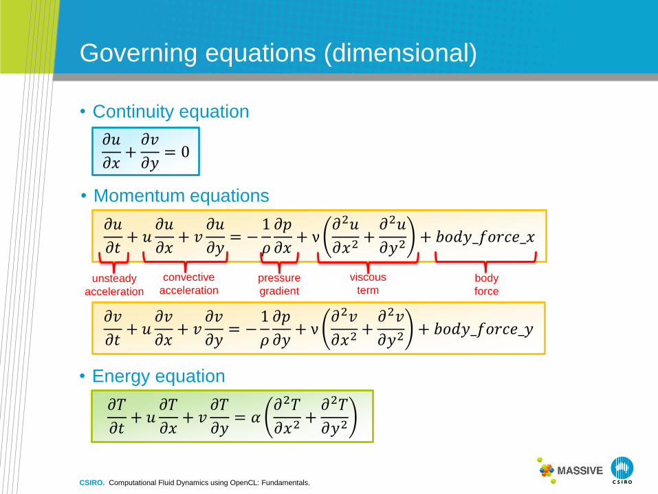
Governing equations (dimensional)

• Continuity equation

𝜕𝑢

𝜕𝑥+𝜕𝑣

𝜕𝑦= 0

𝜕𝑢

𝜕𝑡+ 𝑢

𝜕𝑢

𝜕𝑥+ 𝑣

𝜕𝑢

𝜕𝑦= −

1

𝜌

𝜕𝑝

𝜕𝑥+ ν

𝜕2𝑢

𝜕𝑥2+𝜕2𝑢

𝜕𝑦2+ 𝑏𝑜𝑑𝑦_𝑓𝑜𝑟𝑐𝑒_𝑥

• Momentum equations

𝜕𝑣

𝜕𝑡+ 𝑢

𝜕𝑣

𝜕𝑥+ 𝑣

𝜕𝑣

𝜕𝑦= −

1

𝜌

𝜕𝑝

𝜕𝑦+ ν

𝜕2𝑣

𝜕𝑥2+𝜕2𝑣

𝜕𝑦2+ 𝑏𝑜𝑑𝑦_𝑓𝑜𝑟𝑐𝑒_𝑦

• Energy equation

𝜕𝑇

𝜕𝑡+ 𝑢

𝜕𝑇

𝜕𝑥+ 𝑣

𝜕𝑇

𝜕𝑦= 𝛼

𝜕2𝑇

𝜕𝑥2+𝜕2𝑇

𝜕𝑦2

unsteady

acceleration

convective

acceleration pressure

gradient

viscous

term body

force


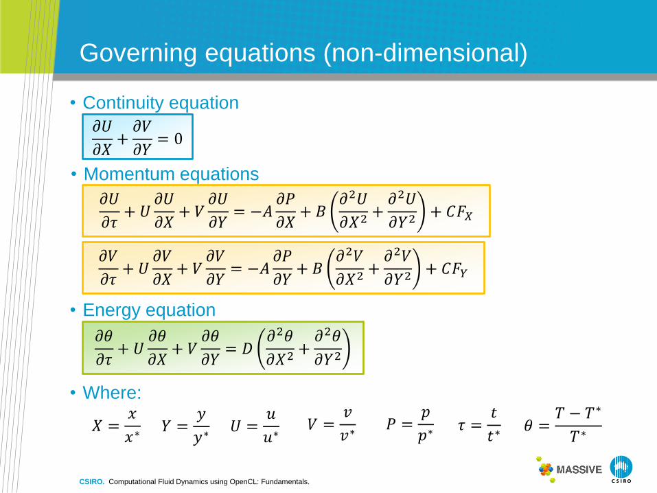
• Continuity equation

𝜕𝑈

𝜕𝑋+𝜕𝑉

𝜕𝑌= 0

Governing equations (non-dimensional)

• Momentum equations

𝜕𝑈

𝜕𝜏+ 𝑈

𝜕𝑈

𝜕𝑋+ 𝑉

𝜕𝑈

𝜕𝑌= −𝐴

𝜕𝑃

𝜕𝑋+ 𝐵

𝜕2𝑈

𝜕𝑋2 +𝜕2𝑈

𝜕𝑌2+ 𝐶𝐹𝑋

𝜕𝑉

𝜕𝜏+ 𝑈

𝜕𝑉

𝜕𝑋+ 𝑉

𝜕𝑉

𝜕𝑌= −𝐴

𝜕𝑃

𝜕𝑌+ 𝐵

𝜕2𝑉

𝜕𝑋2 +𝜕2𝑉

𝜕𝑌2+ 𝐶𝐹𝑌

𝜕𝜃

𝜕𝜏+ 𝑈

𝜕𝜃

𝜕𝑋+ 𝑉

𝜕𝜃

𝜕𝑌= 𝐷

𝜕2𝜃

𝜕𝑋2 +𝜕2𝜃

𝜕𝑌2

• Energy equation

𝑈 =𝑢

𝑢∗

• Where:

𝑉 =𝑣

𝑣∗ 𝑋 =

𝑥

𝑥∗ 𝑌 =

𝑦

𝑦∗ 𝑃 =

𝑝

𝑝∗ 𝜏 =

𝑡

𝑡∗ 𝜃 =

𝑇 − 𝑇∗

𝑇∗


Staggered grid

𝑝𝑖,𝑗 𝑝𝑖+1,𝑗

𝑝𝑖,𝑗+1 𝑝𝑖+1,𝑗+1

𝑣𝑖,𝑗 𝑣𝑖+1,𝑗

𝑣𝑖+1,𝑗+1 𝑣𝑖,𝑗+1

𝑢𝑖,𝑗

𝑢𝑖,𝑗+1

𝑢𝑖+1,𝑗+1

𝑢𝑖+1,𝑗

𝒊 𝒊 + 𝟏

𝒋

𝒋 + 𝟏

𝒄𝒆𝒍𝒍(𝒊, 𝒋)

• Different variables are located at

different locations:

• scalar variables (pressure,

temperature, concentration) are

stored at the centre of the cell,

• the horizontal velocity component is

sampled at the centre of the vertical

cell face,

• the vertical velocity component is

sampled at the centre of the

horizontal cell face.

• The discrete values of u, v and p can be thought as located on three

separate grids, each shifted by half grid spacing to the bottom, to the

left, and to the lower left respectively.

• The staggered arrangement of the unknowns prevents possible

pressure oscillations.


Staggered grid

• In 3D, the grid is set up exactly the same way.


Finite Difference (FD) method

• The continuous problem domain is replaced by a finite-difference

mesh or grid.

𝑈𝑖,𝑗 𝑈𝑖+1,𝑗 𝑈𝑖−1,𝑗

𝑈𝑖,𝑗+1

𝑈𝑖,𝑗−1

∆𝑋

∆𝑌

• If we think about Ui,j as U(X0,Y0) then:

𝑈𝑖+1,𝑗 = 𝑈(𝑋0 + ∆𝑋, 𝑌0)

𝑈𝑖,𝑗+1 = 𝑈(𝑋0, 𝑌0 + ∆𝑌)

𝑈𝑖−1,𝑗 = 𝑈(𝑋0 − ∆𝑋, 𝑌0)

𝑈𝑖,𝑗−1 = 𝑈(𝑋0, 𝑌0 − ∆𝑌)

• The idea of FD representation for derivative can

be introduced by recalling the definition of the

derivative for the function U(X,Y) at X0 and Y0:

𝜕𝑈

𝜕𝑋= lim

∆𝑋→0

𝑈 𝑋0+ ∆𝑋, 𝑌0 − 𝑈(𝑋0, 𝑌0)

∆𝑋

• The difference approximation can be put on a formal basis through

the use of a Taylor-series expansion for U(X0+∆X,Y0) about (X0,Y0):

𝑈 𝑋0+ ∆𝑋, 𝑌0 = 𝑈 𝑋0, 𝑌0 +𝜕𝑈

𝜕𝑋 0

∆𝑋 +𝜕2𝑈

𝜕𝑋2 0

∆𝑋 2

2!+𝜕3𝑈

𝜕𝑋3 0

∆𝑋 3

𝑛!+ ⋯


Computational domain

𝒊 = 𝟎 𝒊 = 𝟏 𝒊 = 𝟐 𝒊 = 𝟑 𝒊 = 𝟒 𝒊 = 𝟓 𝒊 = 𝟔 𝒊 = 𝟕

𝒋 = 𝟒

𝒋 = 𝟑

𝒋 = 𝟐

𝒋 = 𝟏

𝒋 = 𝟎

𝑵𝑿 = 𝟔; 𝑵𝒀 = 𝟑 boundary strip

boundary of computational domain

computational domain

𝑿

𝒀


Computational domain

𝒊 = 𝟎 𝒊 = 𝟏 𝒊 = 𝟐 𝒊 = 𝟑 𝒊 = 𝟒 𝒊 = 𝟓 𝒊 = 𝟔 𝒊 = 𝟕

𝒋 = 𝟒

𝒋 = 𝟑

𝒋 = 𝟐

𝒋 = 𝟏

𝒋 = 𝟎

𝑵𝑿 = 𝟔; 𝑵𝒀 = 𝟑

𝑿

𝒀


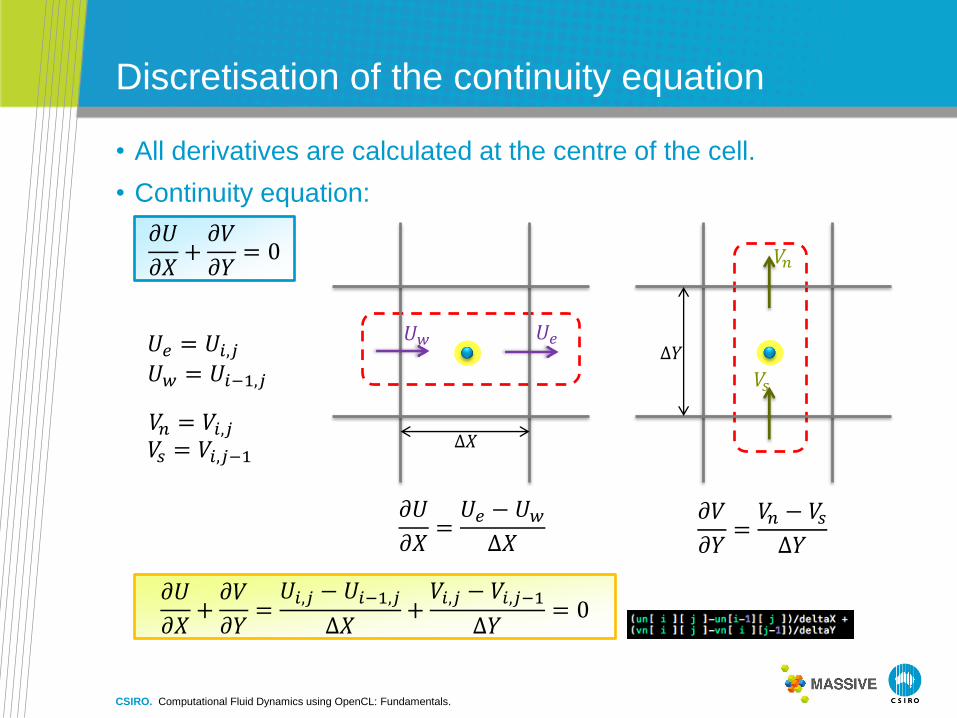
Discretisation of the continuity equation

• Continuity equation:

𝜕𝑈

𝜕𝑋+𝜕𝑉

𝜕𝑌= 0

𝜕𝑈

𝜕𝑋=𝑈𝑒 − 𝑈𝑤∆𝑋

𝜕𝑉

𝜕𝑌=𝑉𝑛 − 𝑉𝑠∆𝑌

𝜕𝑈

𝜕𝑋+𝜕𝑉

𝜕𝑌=𝑈𝑖,𝑗 − 𝑈𝑖−1,𝑗

∆𝑋+𝑉𝑖,𝑗 − 𝑉𝑖,𝑗−1

∆𝑌= 0

• All derivatives are calculated at the centre of the cell.

∆𝑌

𝑉𝑛

𝑉𝑠

∆𝑋

𝑈𝑒 𝑈𝑤 𝑈𝑒 = 𝑈𝑖,𝑗

𝑈𝑤 = 𝑈𝑖−1,𝑗

𝑉𝑛 = 𝑉𝑖,𝑗 𝑉𝑠 = 𝑉𝑖,𝑗−1


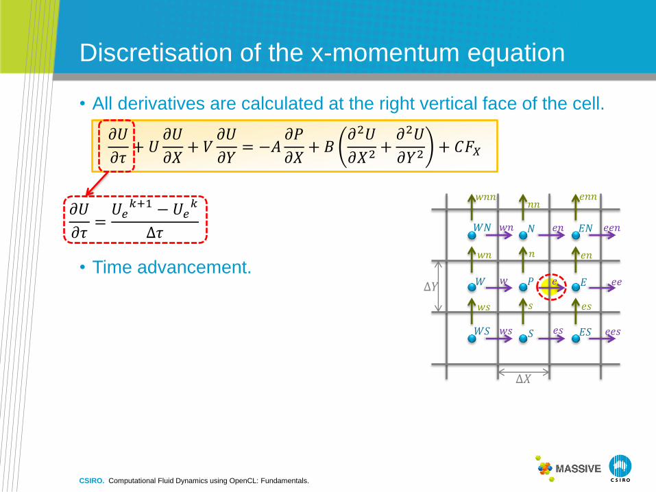
Discretisation of the x-momentum equation

• All derivatives are calculated at the right vertical face of the cell.

𝜕𝑈

𝜕𝜏+ 𝑈

𝜕𝑈

𝜕𝑋+ 𝑉

𝜕𝑈

𝜕𝑌= −𝐴

𝜕𝑃

𝜕𝑋+ 𝐵

𝜕2𝑈

𝜕𝑋2+𝜕2𝑈


𝑃 𝐸 𝑊

𝑁

𝑆

𝐸𝑁

𝐸𝑆

𝑊𝑁

𝑊𝑆

𝑒 𝑤 𝑒𝑒

𝑒𝑛

𝑒𝑠

𝑤𝑛

𝑤𝑠

𝑛

𝑠

𝑛𝑛

𝑤𝑛

𝑤𝑠

𝑒𝑛

𝑒𝑠

𝑤𝑛𝑛 𝑒𝑛𝑛

𝑒𝑒𝑛

𝑒𝑒𝑠

𝜕𝑈

𝜕𝜏=𝑈𝑒

𝑘+1 − 𝑈𝑒𝑘

∆𝜏

∆𝑌

∆𝑋

• Time advancement.




𝜕𝑈

𝜕𝜏+ 𝑈

𝜕𝑈

𝜕𝑋+ 𝑉

𝜕𝑈

𝜕𝑌= −𝐴

𝜕𝑃

𝜕𝑋+ 𝐵

𝜕2𝑈

𝜕𝑋2+𝜕2𝑈


𝑃 𝐸 𝑊

𝑁

𝑆

𝐸𝑁

𝐸𝑆

𝑊𝑁

𝑊𝑆

𝑒 𝑤 𝑒𝑒

𝑒𝑛

𝑒𝑠

𝑤𝑛

𝑤𝑠

𝑛

𝑠

𝑛𝑛

𝑤𝑛

𝑤𝑠

𝑒𝑛

𝑒𝑠


𝑒𝑒𝑛

𝑒𝑒𝑠

𝜕𝑈

𝜕𝜏=𝑈𝑒


∆𝜏

𝐹𝑈𝑋 = 𝑈𝜕𝑈

𝜕𝑋= 𝑈𝑒

𝑈𝑒𝑒 − 𝑈𝑤2∆𝑋

∆𝑌

∆𝑋

• This term can be improved using

upwind scheme !!!




𝜕𝑈

𝜕𝜏+ 𝑈

𝜕𝑈

𝜕𝑋+ 𝑉

𝜕𝑈

𝜕𝑌= −𝐴

𝜕𝑃

𝜕𝑋+ 𝐵

𝜕2𝑈

𝜕𝑋2+𝜕2𝑈


𝑃 𝐸 𝑊

𝑁

𝑆

𝐸𝑁

𝐸𝑆

𝑊𝑁

𝑊𝑆

𝑒 𝑤 𝑒𝑒

𝑒𝑛

𝑒𝑠

𝑤𝑛

𝑤𝑠

𝑛

𝑠

𝑛𝑛

𝑤𝑛

𝑤𝑠

𝑒𝑛

𝑒𝑠


𝑒𝑒𝑛

𝑒𝑒𝑠

𝜕𝑈

𝜕𝜏=𝑈𝑒


∆𝜏


𝜕𝑋= 𝑈𝑒


𝐹𝑈𝑌 = 𝑉𝜕𝑈

𝜕𝑌=

𝑉𝑛 + 𝑉𝑒𝑛 + 𝑉𝑒𝑠 + 𝑉𝑠4

𝑈𝑒𝑛 − 𝑈𝑒𝑠2∆𝑌

∆𝑌

∆𝑋

• This term can be improved using

upwind scheme !!!




𝜕𝑈

𝜕𝜏+ 𝑈

𝜕𝑈

𝜕𝑋+ 𝑉

𝜕𝑈

𝜕𝑌= −𝐴

𝜕𝑃

𝜕𝑋+ 𝐵

𝜕2𝑈

𝜕𝑋2+𝜕2𝑈


𝑃 𝐸 𝑊

𝑁

𝑆

𝐸𝑁

𝐸𝑆

𝑊𝑁

𝑊𝑆

𝑒 𝑤 𝑒𝑒

𝑒𝑛

𝑒𝑠

𝑤𝑛

𝑤𝑠

𝑛

𝑠

𝑛𝑛

𝑤𝑛

𝑤𝑠

𝑒𝑛

𝑒𝑠


𝑒𝑒𝑛

𝑒𝑒𝑠

𝜕𝑈

𝜕𝜏=𝑈𝑒


∆𝜏


𝜕𝑋= 𝑈𝑒



𝜕𝑌=



𝑃𝑅𝐸𝑆𝑆𝑈 = 𝐴𝜕𝑃

𝜕𝑋= 𝐴

𝑃𝐸𝑘+1 − 𝑃𝑃

𝑘+1

∆𝑋

∆𝑌

∆𝑋




𝜕𝑈

𝜕𝜏+ 𝑈

𝜕𝑈

𝜕𝑋+ 𝑉

𝜕𝑈

𝜕𝑌= −𝐴

𝜕𝑃

𝜕𝑋+ 𝐵

𝜕2𝑈

𝜕𝑋2+𝜕2𝑈


𝑃 𝐸 𝑊

𝑁

𝑆

𝐸𝑁

𝐸𝑆

𝑊𝑁

𝑊𝑆

𝑒 𝑤 𝑒𝑒

𝑒𝑛

𝑒𝑠

𝑤𝑛

𝑤𝑠

𝑛

𝑠

𝑛𝑛

𝑤𝑛

𝑤𝑠

𝑒𝑛

𝑒𝑠


𝑒𝑒𝑛

𝑒𝑒𝑠

𝜕𝑈

𝜕𝜏=𝑈𝑒


∆𝜏


𝜕𝑋= 𝑈𝑒



𝜕𝑌=



𝑃𝑅𝐸𝑆𝑆𝑈 = 𝐴𝜕𝑃

𝜕𝑋= 𝐴

𝑃𝐸𝑘+1 − 𝑃𝑃

𝑘+1

∆𝑋

𝐷𝐼𝐹𝐹𝑈 = 𝐵𝑈𝑒𝑒 − 𝑈𝑒

∆𝑋−𝑈𝑒 − 𝑈𝑤∆𝑋

1

∆𝑋+

𝑈𝑒𝑛 − 𝑈𝑒∆𝑌

−𝑈𝑒 − 𝑈𝑒𝑠

∆𝑌

1

∆𝑌

∆𝑌

∆𝑋


𝜕𝑉

𝜕𝜏+ 𝑈

𝜕𝑉

𝜕𝑋+ 𝑉

𝜕𝑉

𝜕𝑌= −𝐴

𝜕𝑃

𝜕𝑌+ 𝐵

𝜕2𝑉

𝜕𝑋2+𝜕2𝑉


Discretisation of the y-momentum equation

𝑃 𝐸 𝑊

𝑁

𝑆

𝐸𝑁

𝐸𝑆

𝑊𝑁

𝑊𝑆

𝑒 𝑤 𝑒𝑒

𝑒𝑛

𝑒𝑠

𝑤𝑛

𝑤𝑠

𝑛

𝑠

𝑛𝑛

𝑤𝑛

𝑤𝑠

𝑒𝑛

𝑒𝑠


𝑒𝑒𝑛

𝑒𝑒𝑠

𝐷𝐼𝐹𝐹𝑉 = 𝐵𝑉𝑒𝑛 − 𝑉𝑛∆𝑋

−𝑉𝑛 − 𝑉𝑤𝑛

∆𝑋

1

∆𝑋+

𝑉𝑛𝑛 − 𝑉𝑛∆𝑌

−𝑉𝑛 − 𝑉𝑠∆𝑌

1

∆𝑌

∆𝑌

∆𝑋 𝑃𝑅𝐸𝑆𝑆𝑉 = 𝐴𝜕𝑃

𝜕𝑌= 𝐴

𝑃𝑁𝑘+1 − 𝑃𝑃

𝑘+1

∆𝑌

𝐹𝑉𝑌 = 𝑉𝜕𝑉

𝜕𝑌= 𝑉𝑛

𝑉𝑛𝑛 − 𝑉𝑠2∆𝑌

𝐹𝑉𝑋 = 𝑈𝜕𝑉

𝜕𝑋=

𝑈𝑤𝑛 + 𝑈𝑒𝑛 + 𝑈𝑒 + 𝑈𝑤4

𝑉𝑒𝑛 − 𝑉𝑤𝑛2∆𝑋

𝜕𝑉

𝜕𝜏=𝑉𝑛

𝑘+1 − 𝑉𝑛𝑘

∆𝜏

• All derivatives are calculated at the upper horizontal face of the cell.


𝜕𝜃

𝜕𝜏+ 𝑈

𝜕𝜃

𝜕𝑋+ 𝑉

𝜕𝜃

𝜕𝑌= 𝐷

𝜕2𝜃

𝜕𝑋2+𝜕2𝜃

𝜕𝑌2

Discretisation of the energy equation

𝑃 𝐸 𝑊

𝑁

𝑆

𝐸𝑁

𝐸𝑆

𝑊𝑁

𝑊𝑆

𝑒 𝑤 𝑒𝑒

𝑒𝑛

𝑒𝑠

𝑤𝑛

𝑤𝑠

𝑛

𝑠

𝑛𝑛

𝑤𝑛

𝑤𝑠

𝑒𝑛

𝑒𝑠


𝑒𝑒𝑛

𝑒𝑒𝑠

𝐷𝐼𝐹𝐹𝑇 = 𝐷𝜃𝐸 − 𝜃𝑃∆𝑋

−𝜃𝑃 − 𝜃𝑊∆𝑋

1

∆𝑋+

𝜃𝑁 − 𝜃𝑃∆𝑌

−𝜃𝑃 − 𝜃𝑆∆𝑌

1

∆𝑌

∆𝑌

∆𝑋

𝜕𝜃

𝜕𝜏=𝜃𝑃

𝑘+1 − 𝜃𝑃𝑘

∆𝜏

• All derivatives are calculated in the centre of the cell.

𝐹𝑇𝑋 = 𝑈𝜕𝜃

𝜕𝑋=

𝑈𝑒 + 𝑈𝑤2

𝜃𝐸 − 𝜃𝑊2∆𝑋

𝐹𝑇𝑌 = 𝑉𝜕𝜃

𝜕𝑌=

𝑉𝑛 + 𝑉𝑠2

𝜃𝑁 − 𝜃𝑆2∆𝑌


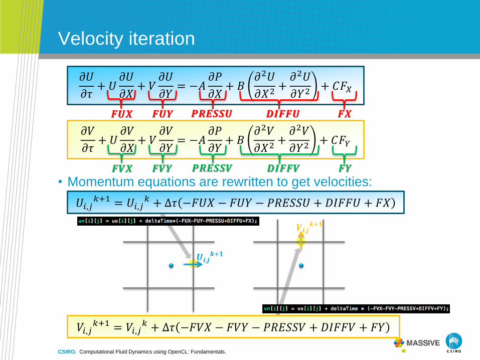
Velocity iteration

𝜕𝑈

𝜕𝜏+ 𝑈

𝜕𝑈

𝜕𝑋+ 𝑉

𝜕𝑈

𝜕𝑌= −𝐴

𝜕𝑃

𝜕𝑋+ 𝐵

𝜕2𝑈

𝜕𝑋2 +𝜕2𝑈


𝜕𝑉

𝜕𝜏+ 𝑈

𝜕𝑉

𝜕𝑋+ 𝑉

𝜕𝑉

𝜕𝑌= −𝐴

𝜕𝑃

𝜕𝑌+ 𝐵

𝜕2𝑉

𝜕𝑋2 +𝜕2𝑉


𝑭𝑼𝑿 𝑭𝑼𝒀 𝑷𝑹𝑬𝑺𝑺𝑼 𝑫𝑰𝑭𝑭𝑼 𝑭𝑿

𝑭𝑽𝑿 𝑭𝑽𝒀 𝑷𝑹𝑬𝑺𝑺𝑽 𝑫𝑰𝑭𝑭𝑽 𝑭𝒀

• Momentum equations are rewritten to get velocities:

𝑈𝑖,𝑗𝑘+1 = 𝑈𝑖,𝑗

𝑘 + ∆𝜏 −𝐹𝑈𝑋 − 𝐹𝑈𝑌 − 𝑃𝑅𝐸𝑆𝑆𝑈 + 𝐷𝐼𝐹𝐹𝑈 + 𝐹𝑋

𝑉𝑖,𝑗𝑘+1 = 𝑉𝑖,𝑗

𝑘 + ∆𝜏 −𝐹𝑉𝑋 − 𝐹𝑉𝑌 − 𝑃𝑅𝐸𝑆𝑆𝑉 + 𝐷𝐼𝐹𝐹𝑉 + 𝐹𝑌

𝑼𝒊,𝒋𝒌+𝟏

𝑽𝒊,𝒋𝒌+𝟏


𝜕𝜃

𝜕𝜏+ 𝑈

𝜕𝜃

𝜕𝑋+ 𝑉

𝜕𝜃

𝜕𝑌= 𝐷

𝜕2𝜃

𝜕𝑋2 +𝜕2𝜃

𝜕𝑌2

Temperature iteration

𝑭𝑻𝑿 𝑭𝑻𝒀 𝑫𝑰𝑭𝑭𝑻

• Energy equation is rewritten to get temperature field:

𝜃𝑖,𝑗𝑘+1 = 𝜃𝑖,𝑗

𝑘 + ∆𝜏 −𝐹𝑇𝑋 − 𝐹𝑇𝑌 + 𝐷𝐼𝐹𝐹𝑈

𝜽𝒊,𝒋𝒌+𝟏

• Energy equation:


OUTER LOOP

Flow Chart of the CPU Fluid Solver

START

Read Configuration

Allocate Memory for Flow

Field Tables

Apply Boundary

Conditions (BC)

Calculate Tentative

Velocities (U, V)

Calculate Pressure

Correction

Correct Pressure and

Velocity Fields, Apply BC

Converged? NO

Calculate Energy

Equation (if required)

YES

Final time

achieved?

Advance All Flow Tables

and Increase Time

NO

Save Results: Flow

Fields, etc...

FINISH

YES

INNER LOOP


HSMAC

• HSMAC (Highly Simplified Marker and Cell): a method to solve

for pressure and velocity components.

𝜕𝑈

𝜕𝜏+ 𝑈

𝜕𝑈

𝜕𝑋+ 𝑉

𝜕𝑈

𝜕𝑌= −𝐴

𝜕𝑃

𝜕𝑋+ 𝐵

𝜕2𝑈

𝜕𝑋2 +𝜕2𝑈


𝜕𝑉

𝜕𝜏+ 𝑈

𝜕𝑉

𝜕𝑋+ 𝑉

𝜕𝑉

𝜕𝑌= −𝐴

𝜕𝑃

𝜕𝑌+ 𝐵

𝜕2𝑉

𝜕𝑋2 +𝜕2𝑉


• Momentum equations:

• Can be rewritten as follows:

𝑈𝑖,𝑗𝑘+1 = 𝑈𝑖,𝑗

𝑘 + ∆𝜏 𝐹𝑖,𝑗𝑘 − 𝐴

𝑃𝑖+1,𝑗𝑘+1 − 𝑃𝑖,𝑗

𝑘+1

∆𝑋

𝑉𝑖,𝑗𝑘+1 = 𝑉𝑖,𝑗

𝑘 + ∆𝜏 𝐺𝑖,𝑗𝑘 − 𝐴

𝑃𝑖,𝑗+1𝑘+1 − 𝑃𝑖,𝑗

𝑘+1

∆𝑌

• Once new pressure are given, we can get new velocity components

from these equations.

Harlow and Welch, Physics of Fluids 8, 2182-2189, 1965. Amsden and Welch, JPC 10, 324-325, 1970.


HSMAC

• These velocity components are required to satisfy the equation of

continuity:

𝜕𝑈

𝜕𝑋+𝜕𝑉

𝜕𝑌= 0

• The solution is sought with the Newton-Raphson method in

stepwise way:

• At first, with the tentative value for pressure, the tentative velocity

components are computed:

𝑚𝑈𝑖,𝑗𝑘+1 = 𝑈𝑖,𝑗

𝑘 + ∆𝜏 𝐹𝑖,𝑗𝑘 − 𝐴

𝑚𝑃𝑖+1,𝑗𝑘+1 − 𝑚𝑃𝑖,𝑗

𝑘+1

∆𝑋

𝑚𝑉𝑖,𝑗𝑘+1 = 𝑉𝑖,𝑗

𝑘 + ∆𝜏 𝐺𝑖,𝑗𝑘 − 𝐴

𝑚𝑃𝑖,𝑗+1𝑘+1 − 𝑚𝑃𝑖,𝑗

𝑘+1

∆𝑌


HSMAC

• The tentative velocity and the pressure fields need to be corrected to

give better approximation at step m+1:

𝑈𝑚+1 𝑘+1 = 𝑈𝑚 𝑘+1 + 𝑈′

𝑉𝑚+1 𝑘+1 = 𝑉𝑚 𝑘+1 + 𝑉′

𝑃𝑚+1 𝑘+1 = 𝑃𝑚 𝑘+1 + 𝑃′

• Then, the LHS of continuity equation is expressed as:

𝐷𝑚+1𝑖,𝑗𝑘+1 =

𝑈𝑚+1𝑖,𝑗𝑘+1 − 𝑈𝑚+1

𝑖−1,𝑗𝑘+1

∆𝑋+

𝑉𝑚+1𝑖,𝑗𝑘+1 − 𝑉𝑚+1

𝑖,𝑗−1𝑘+1

∆𝑌

𝐷𝑚𝑖,𝑗𝑘+1 =

𝑈𝑚𝑖,𝑗𝑘+1 − 𝑈𝑚

𝑖−1,𝑗𝑘+1

∆𝑋+

𝑉𝑚𝑖,𝑗𝑘+1 − 𝑉𝑚

𝑖,𝑗−1𝑘+1

∆𝑌

• The equation of continuity is to be satisfied in the new time step (𝑘 + 1)∆𝜏

so let us assume 𝐷𝑖,𝑗𝑘+1 = 0 though 𝐷𝑖,𝑗

𝑘 ≠ 0 with the non-convergent

incorrect velocity components for 𝑈 and 𝑉.

• Newton-Raphson method provides the stepwise approach for the

solution to satisfy 𝐷𝑖,𝑗𝑘+1 = 0.


HSMAC

• Calculate 𝑃𝑃 so 𝐷𝑃𝑘+1 becomes zero using Newton-Raphson method:

𝑚+1𝑃𝑖,𝑗𝑘+1 = 𝑚 𝑃𝑖,𝑗

𝑘+1 − 𝑚𝐷𝑖,𝑗

𝑘+1

𝑚𝜕𝐷𝑖,𝑗𝜕𝑃𝑖,𝑗

𝑘+1 = 𝑚 𝑃𝑖,𝑗𝑘+1 + 𝑃𝑖,𝑗

′



𝑖−1,𝑗𝑘+1

∆𝑋+


𝑖,𝑗−1𝑘+1

∆𝑌= 𝐷𝐷

• where:

𝑚𝜕𝐷𝑖,𝑗

𝜕𝑃𝑖,𝑗

𝑘+1

= ∆𝜏1

∆𝑋

1

∆𝑋+

1

∆𝑋+

1

∆𝑌

1

∆𝑌+

1

∆𝑌= 𝐷𝐸𝐿

• so:

𝑃𝑖,𝑗′ = −

𝐷𝐷

𝐷𝐸𝐿


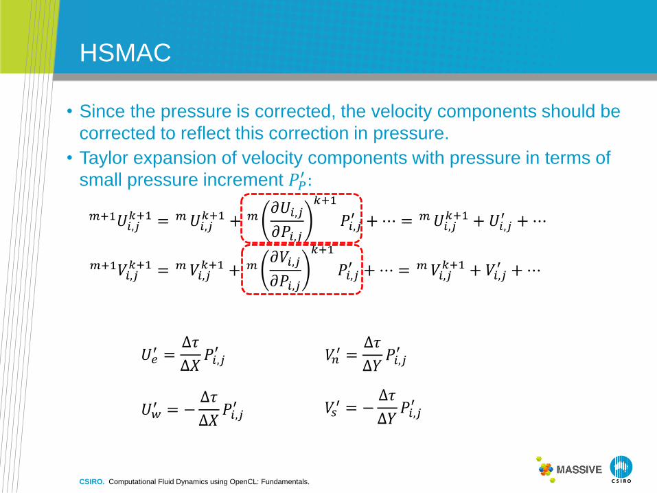
HSMAC

• Since the pressure is corrected, the velocity components should be

corrected to reflect this correction in pressure.

• Taylor expansion of velocity components with pressure in terms of

small pressure increment 𝑃𝑃′ :

𝑚+1𝑈𝑖,𝑗𝑘+1 = 𝑚𝑈𝑖,𝑗

𝑘+1 + 𝑚𝜕𝑈𝑖,𝑗

𝜕𝑃𝑖,𝑗

𝑘+1

𝑃𝑖,𝑗′ +⋯ = 𝑚𝑈𝑖,𝑗

𝑘+1 + 𝑈𝑖,𝑗′ +⋯

𝑚+1𝑉𝑖,𝑗𝑘+1 = 𝑚 𝑉𝑖,𝑗

𝑘+1 + 𝑚𝜕𝑉𝑖,𝑗

𝜕𝑃𝑖,𝑗

𝑘+1

𝑃𝑖,𝑗′ +⋯ = 𝑚 𝑉𝑖,𝑗

𝑘+1 + 𝑉𝑖,𝑗′ +⋯

𝑈𝑒′ =

∆𝜏

∆𝑋𝑃𝑖,𝑗′ 𝑉𝑛

′ =∆𝜏

∆𝑌𝑃𝑖,𝑗′

𝑈𝑤′ = −

∆𝜏

∆𝑋𝑃𝑖,𝑗′ 𝑉𝑠

′ = −∆𝜏



Non-slip boundary conditions

fluid

boundary

wall

• To satisfy the non-slip condition, the continuous velocities should

vanish at the boundary:

U V

𝑈𝑏𝑜𝑢𝑛𝑑𝑎𝑟𝑦 = 0; 𝑉𝑏𝑜𝑢𝑛𝑑𝑎𝑟𝑦 = 0

• Therefore:

𝒊 = 𝟎 𝒊 = 𝟏

𝑈0,𝑗 = 0; 𝑉0,𝑗 = −𝑉1,𝑗

𝒋 𝑈0,𝑗

𝑉0,𝑗 𝑉1,𝑗


Case 1: Lid Driven Cavity

• Used as a validation case for new codes (same here?).

• Fluid is contained in a square cavity with three rigid walls (bottom, left and

right) and one moving wall (top).

𝜕𝑈

𝜕𝜏+ 𝑈

𝜕𝑈

𝜕𝑋+ 𝑉

𝜕𝑈

𝜕𝑌= −

𝜕𝑃

𝜕𝑋+

1

𝑅𝑒

𝜕2𝑈

𝜕𝑋2+𝜕2𝑈

𝜕𝑌2

𝜕𝑉

𝜕𝜏+ 𝑈

𝜕𝑉

𝜕𝑋+ 𝑉

𝜕𝑉

𝜕𝑌= −

𝜕𝑃

𝜕𝑌+

1

𝑅𝑒

𝜕2𝑉

𝜕𝑋2+𝜕2𝑉

𝜕𝑌2

𝜕𝑈

𝜕𝑋+𝜕𝑉

𝜕𝑌= 0

• Reynolds number is a non dimensional parameter that

measure of the ratio of inertial forces to viscous forces:

𝑅𝑒 =

𝑖𝑛𝑒𝑟𝑡𝑖𝑎𝑙 𝑓𝑜𝑟𝑐𝑒

𝑣𝑖𝑠𝑐𝑜𝑢𝑠 𝑓𝑜𝑟𝑐𝑒=𝑈𝐿

𝑣

Ve

locity

field


Case 1: Lid Driven Cavity

Re = 100 Re = 400 Re = 1000

Driven Cavity Test at Re = 1000

-0.7

-0.5

-0.3

-0.1

0.1

0.3

0.5

0.7

0.9

1.1

0 0.1 0.2 0.3 0.4 0.5 0.6 0.7 0.8 0.9 1

x and y location (respectively)

v a

nd

u v

elo

cit

y c

om

po

ne

nts

(re

sp

ec

tiv

ely

)

u- along y=0.5 (Ghia)

u- along y=0.5 (my code)

v- along x=0.5 (my code)

v- along x=0.5 (Ghia)

v- velocity component along y=0.5

u- velocity component along x=0.5

Re = 1000

str

ea

m fu

nctio

n

Ve

locity

field


Accuracy improvements

𝜕𝑈

𝜕𝜏+ 𝑈

𝜕𝑈

𝜕𝑋+ 𝑉

𝜕𝑈

𝜕𝑌= −

𝜕𝑃

𝜕𝑋+

1

𝑅𝑒

𝜕2𝑈

𝜕𝑋2+𝜕2𝑈

𝜕𝑌2

• Upwind (central difference replaced by one sided-differences),

• Upwind + Central Difference,

• QUICK,

Driven Cavity Test at Re = 1000

-0.55

-0.45

-0.35

-0.25

-0.15

-0.05

0.05

0.15

0.25

0.35

0 0.1 0.2 0.3 0.4 0.5 0.6 0.7 0.8 0.9 1

x location

v v

elo

cit

y c

om

po

ne

nt

Ghia

my old FV code (SIMPLE + QUICK)

my code: Central

my code: Upwind

Fluent: Upwind

Fluent: 2nd upwind

my code: Up + Ce

my code: UTOPIA

Driven Cavity at Re = 1000

• UTOPIA:


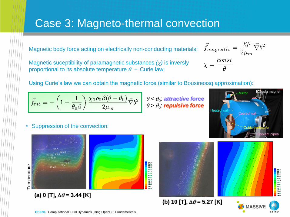
Case 3: Magneto-thermal convection

Magnetic body force acting on electrically non-conducting materials:

Magnetic suceptibility of paramagnetic substances () is inversly

proportional to its absolute temperature q - Curie law:

Using Curie’s law we can obtain the magnetic force (similar to Bousinessq approximation):

q < q0: attractive force

q > q0: repulsive force

• Suppression of the convection:

(a) 0 [T], Dq = 3.44 [K]

(b) 10 [T], Dq = 5.27 [K]

Te

mp

era

ture


Boundary Fitted Coordinates (BFC)

• If we want to solve more complex geometries?

• We need to generate a smooth orthogonal grid system :

• Specify boundaries in the physical plane,

• Solve:

• Or easier:



• Sample grids



𝑅𝑎 = 104; 𝑃𝑟 = 0.71

• Now, if we have our continuity equation in physical plane:

𝜕𝑈

𝜕𝑋+𝜕𝑉

𝜕𝑌= 0

XXX

YYY

2221

1211

aa

aa

Y

X

with transformation between physical and computational plane

• Using chain rules of differential calculus, we have:

YXYX

YX

YXYXJ -

,

,

fa

fa

X

f1211

fa

fa

Y

f2221

the Jacobian of the transformation represents the ratio of the volume

of a grid call in physical space to one in computational space.

fa

faa

fa

faa

XXX

f1211121211112

2

attic space simulation



• Two more sample simulations:


HSMAC on GPU


What is OpenCLTM

Heterogeneous

Computing

Multi-processor

programming, threading

libraries - e.g. OpenMP

Graphics APIs and

Shading Languages,

Vendor Compute APIs

CPUs Multiple cores driving

performance increases

GPUs Increasingly general

purpose data-parallel

computing

Emerging

Intersection

OpenCL - Open Computing Language: open, royalty-free standard for programming

heterogeneous parallel computing at the intersection of GPU and multi-core CPU capabilities.


OpenCL™

• OpenCL (Open Compute Language): an open, royalty-free standard

for parallel programming of heterogeneous systems that include

multi-core processors (CPUs), graphics processing units (GPUs),

and other accelerators such as Cell and digital signal processors

(DSPs).

• OpenCL has complex platform and device management model that

reflects its support for multi-platform and multi-vendor portability.

• Uniform programming environment to write efficient, portable code

for HPC servers, desktop computer systems and handheld devices.

• The standard includes an API for coordinating execution between

devices and a cross-platform parallel programming language.

• Initiated by Apple (now specification editor) and developed by the

Khronos Group.


Design goals of OpenCL

• Enable all compute resources in system

• CPUs, GPUs, and other processors enabled as peers

• Data- and task- parallel compute model

• Efficient parallel programming model

• ANSI C99 based kernel language

• Low-level abstraction

• Abstracts the specifics of the underlying hardware

• High-performance, but device independent

• Define precision requirements for all floating-point computations

• Consistent results on all platforms and devices

• Interoperability with Graphics APIs

• Dedicated support for OpenGL, OpenGL ES and DirectX

• Drive future hardware requirements

• Applicable to both consumer and HPC applications

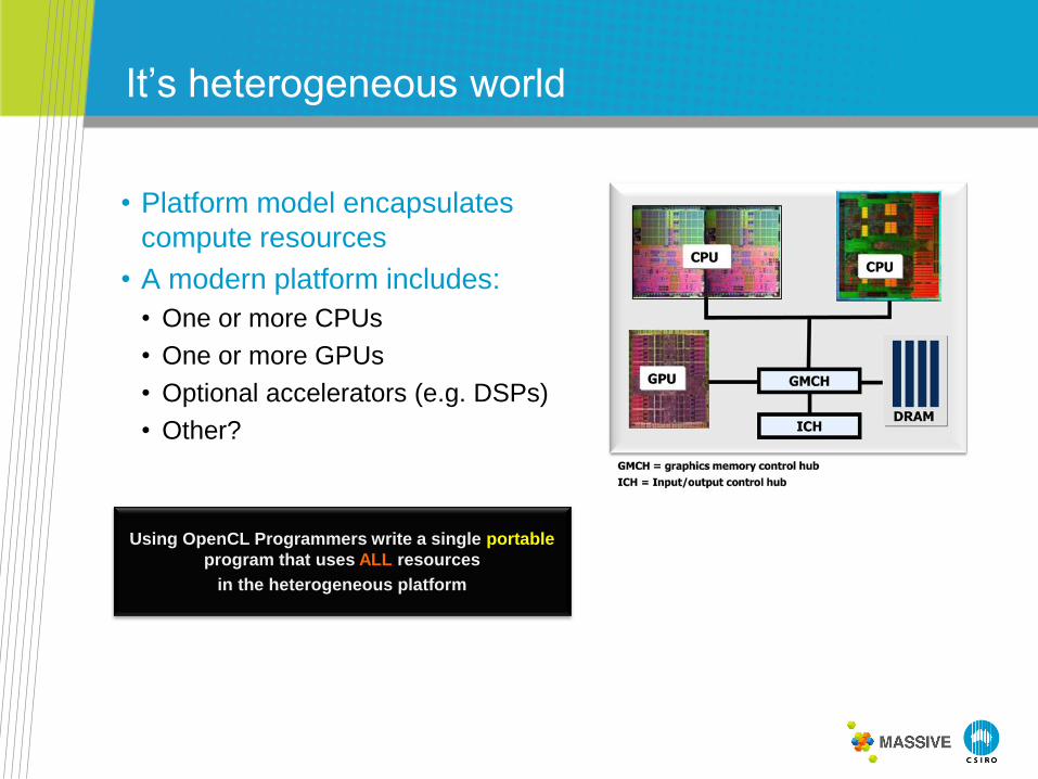
It’s heterogeneous world

• Platform model encapsulates

compute resources

• A modern platform includes:

• One or more CPUs

• One or more GPUs

• Optional accelerators (e.g. DSPs)

• Other?

Using OpenCL Programmers write a single portable

program that uses ALL resources

in the heterogeneous platform

OpenCL Platform Model

• One Host connected to one or more Compute Devices

• Compute device can be a CPU, GPU or other processor

• Each Compute Device is composed of one or more Compute Units

• Compute Unit can may be a core, multi-processor, etc.

• Each Compute Unit is further divided into one or more Processing Elements

• Processing Elements execute code as SIMD or SPMD

COMPUTE UNIT

COMPUTE UNIT

COMPUTE UNIT

COMPUTE UNIT

COMPUTE DEVICE

PROCESSING ELEMENT

COMPUTE UNIT

COMPUTE UNIT

COMPUTE UNIT

COMPUTE DEVICE

..... ….

HOST

CUDA-Enabled GPU

CUDA Streaming Multiprocessor

CUDA Streaming Processor

CPU


Anatomy of OpenCL application

COMPUTE UNIT

COMPUTE UNIT

COMPUTE UNIT

COMPUTE UNIT

COMPUTE DEVICE

COMPUTE UNIT

COMPUTE UNIT

COMPUTE UNIT

COMPUTE DEVICE

.....

…. HOST

OpenCL Application

COMPUTE

DEVICES

Host Code

- Written in C/C++

- Executes on the host

Device Code

- Written in OpenCL C

- Executes on the device

• Host code sends commands to the Devices: • To transfer data between host memory and device memories • To execute device code


Tested GPUs

• GPU Features…

GT 330M QFX4600 QFX4800 460GTX S2050

Streaming Multiprocessors (SM) 6 12 24 7 14

Streaming Processors (SP) / Cores 48 96 192 224 448

Registers per SM 16K 8K 16K 32KB 32KB

Shared Memory per SM 16KB 16KB 16KB 48KB 48KB

Processor Clock [MHz] 990 1200 1204 810 1147

Work item size 512/512/64 512/512/64 512/512/64 1024/1024/64 1024/1024/64

Work group size 512 512 512 1024 1024

CUDA Compute Capability 1.2 1.0 1.3 2.x 2.x


OpenCL execution model 1-D

• Number of work items = 4096:

NDRANGE

DEVICE get_group_id(0) = 2

0 1 2 15

get_global_size(0) = 4096

get_local_size(0) = 256

3 … 4

get_global_id(0) = 1792

WORK GROUP WORK ITEM get_local_id(0) = 255

0 1 … 255

• Number of work items = 4100:

0 1 2 15

get_local_size(0) = 256

3 … 4

0 1 255

16

2 3 … 4

PADDING WASTE

get_global_size(0) = 4352

(A kernel is executed in each point of a problem domain)

__kernel void

addVector(__global const float *A,

__global const float *B,

__global float *C,

int N)

{

int index = get_global_id(0);

if (index < N)

C[index] = A[index]+B[index];

}


OpenCL execution model 2-D

• Number of work items to execute 128 x 128 = 16384:

NDRANGE

DEVICE

0,0 1,0 2,0

0,1

0,2

1,1

…

…

7,0

7,7 0,7

3,4

0,0 1,0 2,0

0,1

0,2

1,1

…

…

15,0

0,15

c

WORK GROUP WORK ITEMS

2,2

4,1

get_global_size(0)

ge

t_glo

bal_

siz

e(1

) ge

t_lo

ca

l_siz

e(1

)

get_local_size(0)

get_group_id(0),get_group_id(1)

get_local_id(0),get_local_id(1) get_global_id(0),get_global_id(1)

.

(A kernel is executed in each point of a problem domain)


HOST OUTER LOOP

Flow Chart of the OpenCL Fluid Solver

START

Read Configuration

Allocate Memory for Flow

Field Tables

Apply Boundary

Conditions (BC)

Calculate Tentative

Velocities (U, V)

Calculate Pressure

Correction

Correct Pressure and

Velocity Fields, Apply BC

Converged? NO

Calculate Energy

Equation (if required)

YES Final time

achieved?

Advance All Flow Tables

and Increase Time

NO

Save Results: Flow

Fields, etc...

FINISH

YES

HOST INNER LOOP

Get OpenCL Platform,

Initialize Device, Create

Context, Create

Command Queue

Create OCL Memory

Buffers

Create OCL Program,

Create Kernels and Set

Kernel Arguments

Setup Boundary Flags

Copy Host Memory

Buffers to GPU Buffers

krnl_bc_u krnl_bc_v krnl_bc_p

krnl_momentum_u krnl_momentum_v

krnl_pressure_velocity_correction

krnl_bc_u krnl_bc_v krnl_bc_p

krnl_energy

krnl_advance_u krnl_advance_v

Copy GPU Buffers to

Host Memory Buffers

Release Command

Queue, Context, Kernels,

Programs, Memory

Visualisation


Before we start…

• Get OpenCL platform and initialise computing devices:

• Create context and create command queue.


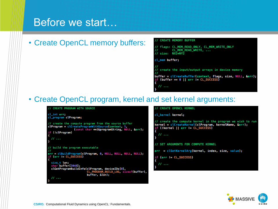
Before we start…

• Create OpenCL program, kernel and set kernel arguments:

• Create OpenCL memory buffers:


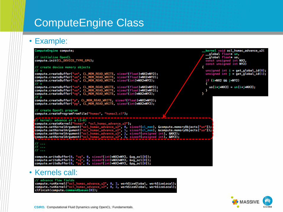
ComputeEngine Class

• Example:

• Kernels call:


Boundary Conditions on GPU

• Setup boundary conditions

• Create cells with boundary flags for velocity, pressure, temperature

and concentration fields.

• Below: boundary flags for cells to assist scalar computations.

𝒊 = 𝟎 𝒊 = 𝟏 𝒊 = 𝟐 𝒊 = 𝟑 𝒊 = 𝟒 𝒊 = 𝟔 𝒊 = 𝟕

𝒋 = 𝟒

𝒋 = 𝟑

𝒋 = 𝟐

𝒋 = 𝟏

𝒋 = 𝟎

𝒊 = 𝟓

𝒇𝒍𝒂𝒈 = 𝟏

𝒇𝒍𝒂𝒈 = 𝟑

𝒇𝒍𝒂𝒈 = 𝟒

𝒇𝒍𝒂𝒈 = 𝟐

𝒅𝒐𝒎𝒂𝒊𝒏

𝑵𝑿 = 𝟔; 𝑵𝒀 = 𝟑

𝑵𝑿𝟐 = 𝟖; 𝑵𝒀𝟐 = 𝟓


Boundary conditions on GPU

𝟎 𝟏 𝟐 𝟑 𝟒 𝟓 𝟔 𝟕

𝟒

𝟑

𝟐

𝟏

𝟎

𝟎 𝟏 𝟐 𝟑 𝟒 𝟓 𝟔 𝟕

𝟏

𝟐

𝟑

𝟒

−𝟏

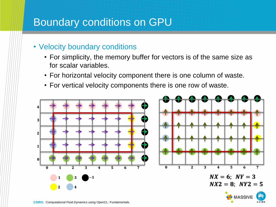
• Velocity boundary conditions

• For simplicity, the memory buffer for vectors is of the same size as

for scalar variables.

• For horizontal velocity component there is one column of waste.

• For vertical velocity components there is one row of waste.

𝑵𝑿 = 𝟔; 𝑵𝒀 = 𝟑

𝑵𝑿𝟐 = 𝟖; 𝑵𝒀𝟐 = 𝟓


Memory Buffers Structure

𝟎 𝟏 𝟐 𝟑 𝟒 𝟎 𝟏 𝟐 𝟑 𝟒 𝒊 = 𝟎 𝒊 = 𝟏 𝒊 = 𝟐 𝒊 = 𝟑 𝒊 = 𝟒

𝒋 = 𝟒

𝒋 = 𝟑

𝒋 = 𝟐

𝒋 = 𝟏

𝒋 = 𝟎

𝑵𝑿 = 𝟑; 𝑵𝒀 = 𝟑; 𝑵𝑿𝟐 = 𝟓; 𝑵𝒀𝟐 = 𝟓

P

PG

UN, UO

UG

VN, VO

VG

CSIRO. Numerical Simulations in Fluid Dynamics using GPU: a Practical Introduction.

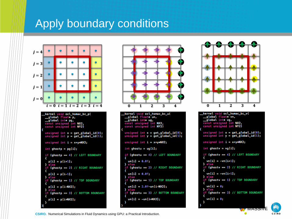
Apply boundary conditions

𝟎 𝟏 𝟐 𝟑 𝟒 𝟎 𝟏 𝟐 𝟑 𝟒 𝒊 = 𝟎 𝒊 = 𝟏 𝒊 = 𝟐 𝒊 = 𝟑 𝒊 = 𝟒

𝒋 = 𝟒

𝒋 = 𝟑

𝒋 = 𝟐

𝒋 = 𝟏

𝒋 = 𝟎

CSIRO. Numerical Simulations in Fluid Dynamics using GPU: a Practical Introduction.

Calculate tentative velocity component U

𝜕𝑈

𝜕𝜏+ 𝑈

𝜕𝑈

𝜕𝑋+ 𝑉

𝜕𝑈

𝜕𝑌= −𝐴

𝜕𝑃

𝜕𝑋+ 𝐵

𝜕2𝑈

𝜕𝑋2 +𝜕2𝑈

𝜕𝑌2

𝑈𝑖,𝑗𝑘+1=

𝑈𝑖,𝑗𝑘 + ∆𝜏 −𝐹𝑈𝑋 − 𝐹𝑈𝑌 − 𝑃𝑅𝐸𝑆𝑆𝑈 + 𝐷𝐼𝐹𝐹𝑈

• From X- momentum equation

𝑃 𝐸 𝑊

𝑁

𝑆

𝐸𝑁

𝐸𝑆

𝑊𝑁

𝑊𝑆

𝑒 𝑤 𝑒𝑒

𝑒𝑛

𝑒𝑠

𝑤𝑛

𝑤𝑠

𝑛

𝑠

𝑛𝑛

𝑤𝑛

𝑤𝑠

𝑒𝑛

𝑒𝑠


𝑒𝑒𝑛

𝑒𝑒𝑠

∆𝑌

∆𝑋


𝑃 𝐸 𝑊

𝑁

𝑆

𝐸𝑁

𝐸𝑆

𝑊𝑁

𝑊𝑆

𝑒 𝑤 𝑒𝑒

𝑒𝑛

𝑒𝑠

𝑤𝑛

𝑤𝑠

𝑛

𝑠

𝑛𝑛

𝑤𝑛

𝑤𝑠

𝑒𝑛

𝑒𝑠


𝑒𝑒𝑛

𝑒𝑒𝑠

∆𝑌

∆𝑋

𝑉𝑖,𝑗𝑘+1 =

𝑉𝑖,𝑗𝑘 + ∆𝜏 −𝐹𝑉𝑋 − 𝐹𝑉𝑌 − 𝑃𝑅𝐸𝑆𝑆𝑉 + 𝐷𝐼𝐹𝐹𝑉

𝜕𝑉

𝜕𝜏+ 𝑈

𝜕𝑉

𝜕𝑋+ 𝑉

𝜕𝑉

𝜕𝑌= −𝐴

𝜕𝑃

𝜕𝑌+ 𝐵

𝜕2𝑉

𝜕𝑋2 +𝜕2𝑉

𝜕𝑌2

Calculate tentative velocity component V

• From X- momentum equation


Pressure and velocity corrections



𝑖−1,𝑗𝑘+1

∆𝑋+


𝑖,𝑗−1𝑘+1

∆𝑌= 𝐷

𝑚𝜕𝐷𝑖,𝑗

𝜕𝑃𝑖,𝑗

𝑘+1

=

∆𝜏1

∆𝑋

1

∆𝑋+

1

∆𝑋+

1

∆𝑌

1

∆𝑌+

1

∆𝑌= 𝐷𝐸𝐿

𝑈𝑒′ =

∆𝜏

∆𝑋𝑃𝑖,𝑗′

𝑉𝑛′ =

∆𝜏


𝑈𝑤′ = −

∆𝜏

∆𝑋𝑃𝑖,𝑗′

𝑉𝑠′ = −

∆𝜏


𝑃𝑃′ = −

𝐷

𝐷𝐸𝐿

𝑃 𝐸 𝑊

𝑁

𝑆

𝐸𝑁

𝐸𝑆

𝑊𝑁

𝑊𝑆

𝑒 𝑤 𝑒𝑒

𝑒𝑛

𝑒𝑠

𝑤𝑛

𝑤𝑠

𝑛

𝑠

𝑛𝑛

𝑤𝑛

𝑤𝑠

𝑒𝑛

𝑒𝑠


𝑒𝑒𝑛

𝑒𝑒𝑠

∆𝑌

∆𝑋


0

500

1000

1500

2000

2500

0 64 128 192 256 320

Tim

e [

s]

Number of cells (K)

S2050

GT 330M

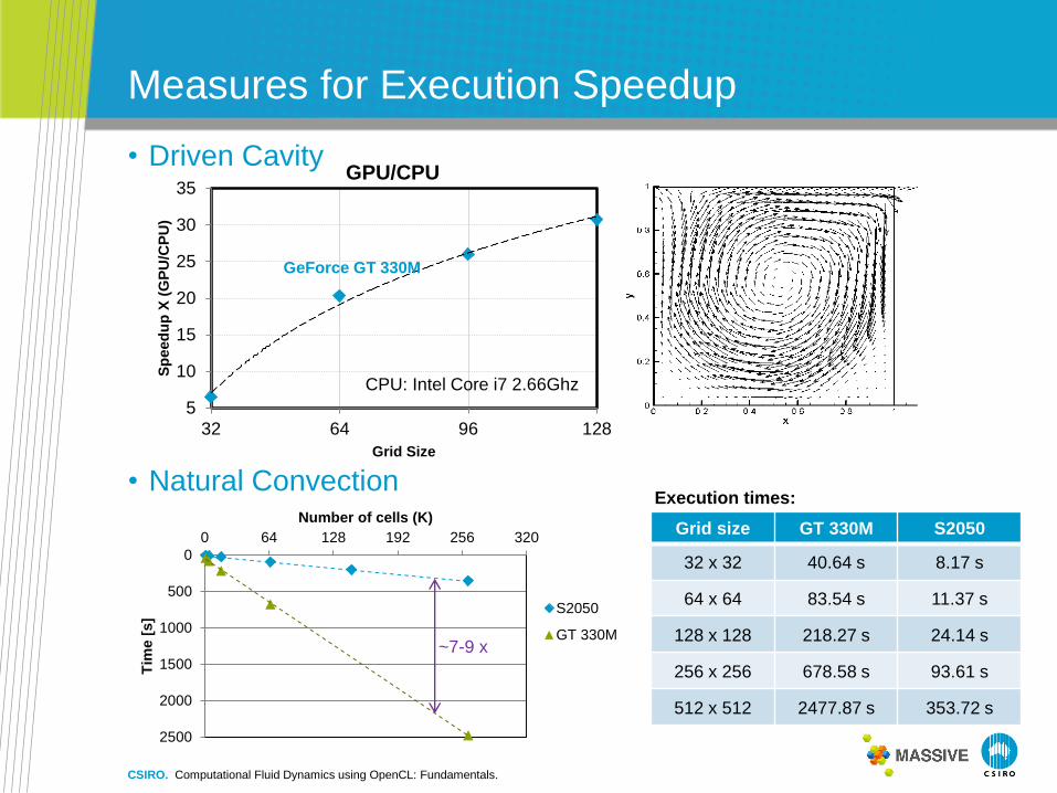
Measures for Execution Speedup

• Driven Cavity

5

10

15

20

25

30

35

32 64 96 128

Sp

eed

up

X (

GP

U/C

PU

)

Grid Size

GPU/CPU

GeForce GT 330M

• Natural Convection

CPU: Intel Core i7 2.66Ghz

~7-9 x

Grid size GT 330M S2050

32 x 32 40.64 s 8.17 s

64 x 64 83.54 s 11.37 s

128 x 128 218.27 s 24.14 s

256 x 256 678.58 s 93.61 s

512 x 512 2477.87 s 353.72 s

Execution times:


Summary

• CFD does not need to be scary !!!

• We used the following approach:

• Equations Discretisation Implementation Verification

Results Transfer CPU code to GPU code Verification

Results.

• Methods presented:

• Finite Difference Method (for discretisation),

• HSMAC Method (for mutual iteration of pressure/velocity fields),

• BFC (for solving Navier-Stokes equations on complex geometry),

• Upwind and UTOPIA (for getting more stable and accurate results),

• OpenCL (for speeding-up computing process).

• The methodology presented, can be extended into 3D and

applied to compute different cases in real-time, e.g., smoke,

free surface flows, ventilation, turbulent flows, etc.

• Source-code to be released online.


Contact Us

Phone: 1300 363 400 or +61 3 9545 2176

Email: [email protected] Web: www.csiro.au

Thank you… …

Mathematics, Informatics & Statistics

Dr Tomasz P Bednarz

Research Scientist

Phone: +61 437 625 623

Email: [email protected]

Web: www.csiro.au/org/CESRE.html

www.tomaszbednarz.com

Acknowledgments: Dr J.Taylor, C.Caris, Prof. H.Ozoe, Prof. H.Hirano, Prof. T.Tagawa, Prof. J.C.Patterson,

Prof. Chengwang Lei, Dr Wenxian Lin, Prof. J.S.Szmyd, Dr P.Cleary, Dr M.Rudman, Dr

J.Ralston, Dr L.Domanski, Dr J.Malos, J.Craig, Dr S.Zawlodzka-Bednarz

computational fluid dynamics using opencl: fundamentals · pdf filefluid dynamics •...

Documents