Computational Logic

Prolog Programming Basics

1

Overview

1. Using unification

2. Data structures

3. Recursion, backtracking, and search

4. Control of execution

2

Role of Unification in Execution

• As mentioned before, unification used to access data and give values to variables.

Example: Consider query ?- animal(A), named(A,Name). with:

animal(dog(barry)).

named(dog(Name),Name).

Execution of animal(A) assigns a (ground) value to A.

Execution of named(A,Name) assigns a (ground) value to Name by accessing the

data in the subfield of the dog/1 structure.

• Also, unification is used to pass parameters in procedure calls and to return

values upon procedure exit.

?- animal(A), named(A,Name) returns a value upon exit of animal(A)

?- named(dog(barry),Name) passes a value in first argument

of call to named/2

Name = barry returns a value in second argument

on exit of named/2

3

Modes

• In fact, argument positions are not fixed a priory to be input or output.

Example: Consider query ?- pet(spot). vs. ?- pet(X).

• Upon a call to a procedure, any argument may be ground, free, or partially

instantiated.

• Thus, procedures can be used in different modes

(different sets of arguments are input or output in each mode).

Example: Consider the following queries:

?- named(dog(barry),Name). ?- named(A,barry).

?- named(dog(barry),barry). ?- named(A,Name).

• An argument may even be both input and output.

Example: Consider query ?- struct(f(A,b)). with:

struct(f(a,B)).

4

Logical Equivalence: Reversible Computations

• The fact that predicates can be called in any mode is a direct consequence of

their logical nature.

⋄ By definition: plus(X,Y,Z) ⇔ Z = X + Y (math. addition)

⋄ From mathematics: Z = X + Y ⇔ X = Z− Y ⇔ Y = Z− X

⋄ Thus: plus(X,Y,Z) ⇔ X = Z− Y ⇔ Y = Z− X

• Computationally:

Mathematical Functional (Abused)

Meaning Characterization Predicate Mode Sample Query Answer

Z = X + Y Z = add(X,Y) plus(+,+,-) ?- plus(2,1,Z). Z = 3

X = Z− Y X = sub(Z,Y) plus(-,+,+) ?- plus(X,1,3). X = 2

Y = Z− X Y = sub(Z,X) plus(+,-,+) ?- plus(2,Y,3). Y = 1

5

Accessing Data

• Accesing subfields of records:

Example:

day(date(Day,_Month,_Year),Day).

month(date(_Day,Month,_Year),Month).

year(date(_Day,_Month,Year),Year).

• Naming subfields:

Example:

date(day, date(Day,_Month,_Year),Day).

date(month,date(_Day,Month,_Year),Month).

date(year, date(_Day,_Month,Year),Year).

6

Accessing Data (Contd.)

• Initializing variables:

Example: ?- init(X), ...

init(date(9,6,2011)).

• Comparing values:

Example: ?- init_1(X), init_2(Y), equal(X,Y).

equal(X,X).

or simply: ?- init_1(X), init_2(X).

7

Structured Data and Data Abstraction (and the ’=’ Predicate)

• Data structures are created using (complex) terms.

• Structuring data is important:

course(complog,wed,18,30,20,30,’F.’,’Bueno’,new,5102).

• When is the Computational Logic course?

?- course(complog,Day,StartH,StartM,FinishH,FinishM,C,D,E,F).

• Structured version:

course(complog,Time,Lecturer, Location) :-

Time = t(wed,18:30,20:30),

Lecturer = lect(’F.’,’Bueno’),

Location = loc(new,5102).

Note: “X=Y” is equivalent to “=(X,Y)”

where the predicate =/2 is defined as the fact “=(X,X).” – Plain unification!

• Equivalent to:

course(complog, t(wed,18:30,20:30),

lect(’F.’,’Bueno’), loc(new,5102)).

8

Structured Data and Data Abstraction (and The Anonymous Variable)

• Given:

course(complog,Time,Lecturer, Location) :-

Time = t(wed,18:30,20:30),

Lecturer = lect(’F.’,’Bueno’),

Location = loc(new,5102).

• When is the Computational Logic course?

?- course(complog,Time, A, B).

has solution:

{Time=t(wed,18:30,20:30), A=lect(’F.’,’Bueno’), B=loc(new,5102)}

• Using the anonymous variable (“ ”):

?- course(complog,Time, , ).

has solution:

{Time=t(wed,18:30,20:30)}

9

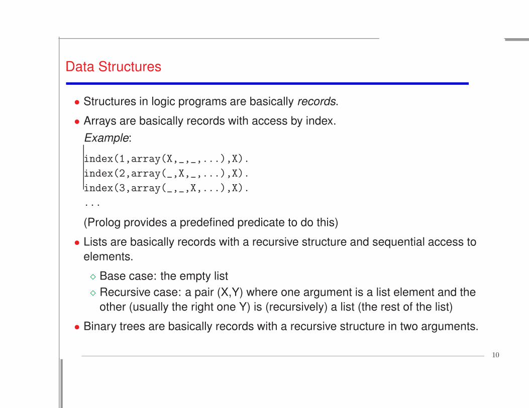
Data Structures

• Structures in logic programs are basically records.

• Arrays are basically records with access by index.

Example:

index(1,array(X,_,_,...),X).

index(2,array(_,X,_,...),X).

index(3,array(_,_,X,...),X).

...

(Prolog provides a predefined predicate to do this)

• Lists are basically records with a recursive structure and sequential access to

elements.

⋄ Base case: the empty list

⋄ Recursive case: a pair (X,Y) where one argument is a list element and the

other (usually the right one Y) is (recursively) a list (the rest of the list)

• Binary trees are basically records with a recursive structure in two arguments.

10

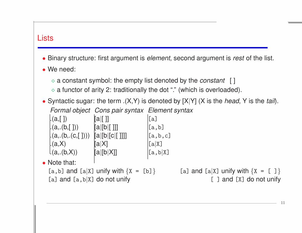
Lists

• Binary structure: first argument is element, second argument is rest of the list.

• We need:

⋄ a constant symbol: the empty list denoted by the constant [ ]

⋄ a functor of arity 2: traditionally the dot “.” (which is overloaded).

• Syntactic sugar: the term .(X,Y) is denoted by [X|Y] (X is the head, Y is the tail).

Formal object Cons pair syntax Element syntax

.(a,[ ]) [a|[ ]] [a]

.(a,.(b,[ ])) [a|[b|[ ]]] [a,b]

.(a,.(b,.(c,[ ]))) [a|[b|[c|[ ]]]] [a,b,c]

.(a,X) [a|X] [a|X]

.(a,.(b,X)) [a|[b|X]] [a,b|X]

• Note that:

[a,b] and [a|X] unify with {X = [b]} [a] and [a|X] unify with {X = [ ]}

[a] and [a,b|X] do not unify [ ] and [X] do not unify

11

Strings (Lists of codes) (and Comments)

• Strings (of characters): in between "...".

If " belongs to the string then escape it (duplicate it).

Examples: "Prolog" "This is a ""string"""

• Simply syntactic sugar: equivalent to the corresponding list of ASCII character

codes.

"Prolog" ≡ [80,114,111,108,111,103]

• Comments:

⋄ Using “%”: rest of line is a comment.

⋄ Using “/* ... */”: everything in between is a comment.

12

Lists (member)

• member(X,Y) iff X is a member of list Y.

• By generalization:member(a,[a]). member(b,[b]). etc. ⇒ member(X,[X]).

member(a,[a,c]). member(b,[b,d]). etc. ⇒ member(X,[X,Y]).

member(a,[a,c,d]). member(b,[b,d,l]).etc. ⇒ member(X,[X,Y,Z]).

⇒ member(X,[X|Y]).

member(a,[c,a]), member(b,[d,b]). etc. ⇒ member(X,[Y,X]).

member(a,[c,d,a]). member(b,[s,t,b]). etc. ⇒ member(X,[Y,Z,X]).

⇒ member(X,[Y|Z]) :- member(X,Z).

• Resulting definition:

member(X,[X| ]).

member(X,[ |T]) :- member(X,T).

13

Lists (member) (Contd.)

• Resulting definition:

member(X,[X| ]).

member(X,[ |T]) :- member(X,T).

• Uses of member(X,Y):

⋄ checking whether an element is in a list: ?- member(b,[a,b,c]).

⋄ finding an element in a list: ?- member(X,[a,b,c]).

⋄ finding a list containing an element: ?- member(a,Y).

• Define:

⋄ select(X,Ys,Zs) : X is an element of the list Ys and Zs is the list of the other

elements of Ys.

⋄ include(X,Ys,Zs) : Zs is the list resulting from including element X into list Ys

(in any place).

14

Lists (append)

• Concatenation of lists: append(X,Y,Z) iff Z = X.Y

(“.” is an operator for list concatenation)

• By generalization (recurring on the first argument):

⋄ Base case:

append([],[a],[a]). append([],[a,b],[a,b]). etc.

⇒ append([],Ys,Ys).

⋄ Rest of cases (first step):

append([a],[b],[a,b]).

append([a],[b,c],[a,b,c]). etc.

⇒ append([X],Ys,[X|Ys]).

append([a,b],[c],[a,b,c]).

append([a,b],[c,d],[a,b,c,d]). etc.

⇒ append([X,Z],Ys,[X,Z|Ys]).

This is still infinite → we need to generalize more.

15

Lists (append) (Contd.)

• Second generalization:

append([X],Ys,[X|Ys]).

append([X,Z],Ys,[X,Z|Ys]).

append([X,Z,W],Ys,[X,Z,W|Ys]).

⇒ append([X|Xs],Ys,[X|Zs]) :- append(Xs,Ys,Zs).

• So, we have:

append([],Ys,Ys).

append([X|Xs],Ys,[X|Zs]) :- append(Xs,Ys,Zs).

• Uses of append:

⋄ concatenate two given lists: ?- append([a,b],[c],Z).

⋄ find differences between lists: ?- append(X,[c],[a,b,c]).

⋄ split a list: ?- append(X,Y,[a,b,c]).

16

Recursion and Induction

• Recursion is logical induction.

• append(Xs,Ys,Zs) by induction:

(on one of the arguments, e.g. Xs)

⋄ Base: Xs=[]

* Zs=Xs.Ys if Zs=Ys

⋄ Hypothesis: Xs=[X|Xs1] and

we already have Zs1=Xs1.Ys1

⋄ Step: Xs=[X|Xs1] and

we would have Zs=Xs.Ys if:

* Ys=Ys1

* Zs=[X|Zs1]

• Resulting definition:

append([],Ys,Ys).

append([X|Xs1],Ys,[X|Zs1]) :- append(Xs1,Ys,Zs1).

17

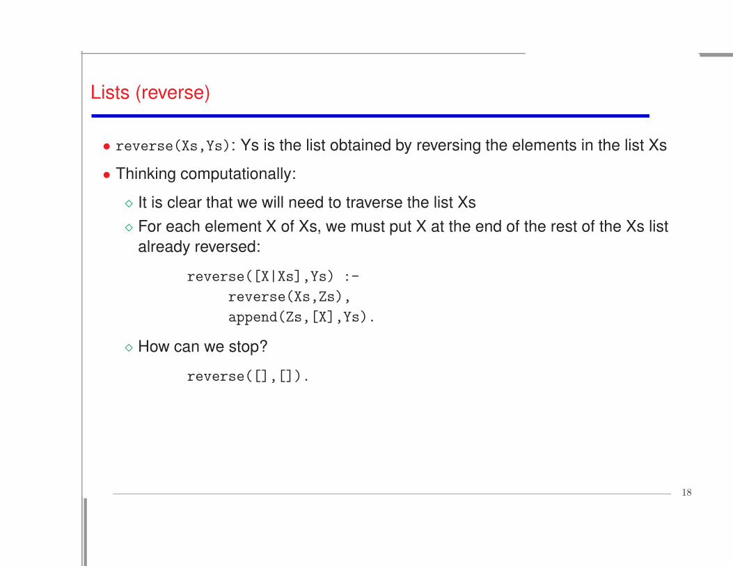
Lists (reverse)

• reverse(Xs,Ys): Ys is the list obtained by reversing the elements in the list Xs

• Thinking computationally:

⋄ It is clear that we will need to traverse the list Xs

⋄ For each element X of Xs, we must put X at the end of the rest of the Xs list

already reversed:

reverse([X|Xs],Ys) :-

reverse(Xs,Zs),

append(Zs,[X],Ys).

⋄ How can we stop?

reverse([],[]).

18

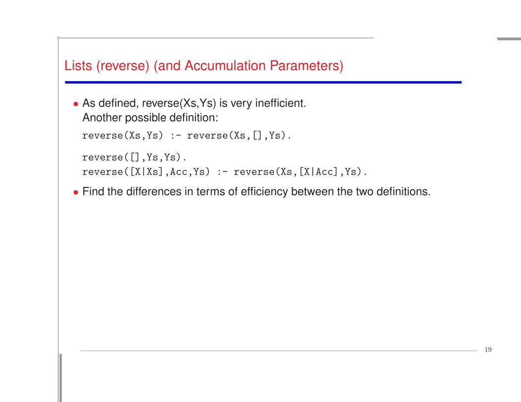
Lists (reverse) (and Accumulation Parameters)

• As defined, reverse(Xs,Ys) is very inefficient.

Another possible definition:

reverse(Xs,Ys) :- reverse(Xs,[],Ys).

reverse([],Ys,Ys).

reverse([X|Xs],Acc,Ys) :- reverse(Xs,[X|Acc],Ys).

• Find the differences in terms of efficiency between the two definitions.

19

Lists (Exercises)

• Define prefix(X,Y) : the list X is a prefix of the list Y, e.g.

prefix([a, b], [a, b, c, d])

• Define suffix(X,Y) : the list X is a suffix of the list Y.

• Define sublist(X,Y) : the elements of list X occur within list Y in the same order

and contiguous.

• Define sublist(X,Y) : the elements of list X occur within list Y in the same order

(maybe not contiguous).

• Define sublist(X,Y) : the elements of list X occur within list Y (maybe not in the

same order nor contiguous).

• Define length(Xs,N) : N is the length of the list Xs

(use Peano representation for natural numbers)

20

Incomplete Data Structures

• Example – difference lists:

⋄ A pair X-Y where X is an open-ended list finished in Y, which is a free variable.

Example: [1,2,3,4|X]-X

(actually, the pair is usually not explicit, instead there is a couple of arguments

that is acting as a difference list)

⋄ Allows us to keep a pointer to the end of the list.

⋄ Allows appending in constant time:

append_dl(X-Y,Y-Z,X-Z).

(actually, no call to append dl is normally necessary)

⋄ But can only be done once...

• Also difference trees, open-ended lists and trees, dictionaries, queues, ...

21

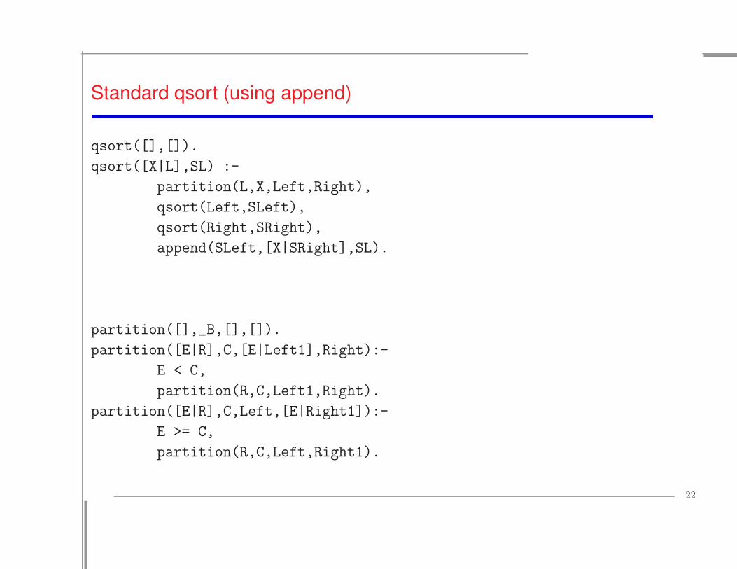
Standard qsort (using append)

qsort([],[]).

qsort([X|L],SL) :-

partition(L,X,Left,Right),

qsort(Left,SLeft),

qsort(Right,SRight),

append(SLeft,[X|SRight],SL).

partition([],_B,[],[]).

partition([E|R],C,[E|Left1],Right):-

E < C,

partition(R,C,Left1,Right).

partition([E|R],C,Left,[E|Right1]):-

E >= C,

partition(R,C,Left,Right1).

22

qsort w/Difference Lists (no append!)

• First list is normal list, second is built as a difference list.

dlqsort(L,SL) :- dlqsort_(L,SL,[]).

dlqsort_([],R,R).

dlqsort_([X|L],SL,R) :-

partition(L,X,Left,Right),

dlqsort_(Left,SL,[X|SR]),

dlqsort_(Right,SR,R).

% Partition is the same as before.

23

Backtracking and Search

• Backtracking allows exploring the different execution paths until a solution is

found.

• Execution of a query is in a fact a search of a solution to the query.

X=[ ]X=[1,2,1,2]

X=[1,2][1,2]=[1,2]

X=[1][1]=[2,1,2]

X=[1,2,1][1,2,1]=[2]

append(X,X,[1,2,1,2])

append([ ],Ys,Ys) append(Y,[1|Y],[2,1,2])

append(Z,[1,2|Z],[1,2])

append(A,[1,2,1|A],[2])

append(B,[1,2,1,2|B],[ ])

append([ ],Ys,Ys)

append([ ],Ys,Ys)

append([ ],Ys,Ys)

X=[1|Y]

Y=[2|Z]

Z=[1|A]

A=[2|B]

append([ ],Ys,Ys)

X=[1,2,1,2][1,2,1,2]=[ ]

fail

24

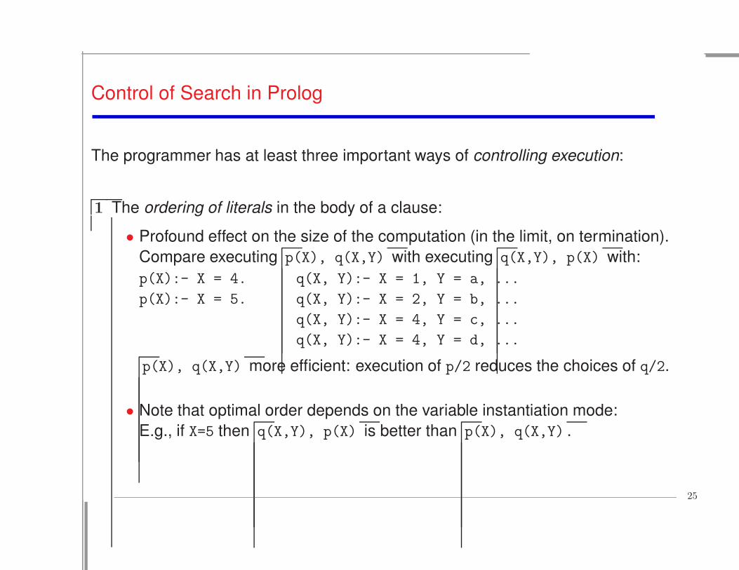
Control of Search in Prolog

The programmer has at least three important ways of controlling execution:

1 The ordering of literals in the body of a clause:

• Profound effect on the size of the computation (in the limit, on termination).

Compare executing p(X), q(X,Y) with executing q(X,Y), p(X) with:

p(X):- X = 4. q(X, Y):- X = 1, Y = a, ...

p(X):- X = 5. q(X, Y):- X = 2, Y = b, ...

q(X, Y):- X = 4, Y = c, ...

q(X, Y):- X = 4, Y = d, ...

p(X), q(X,Y) more efficient: execution of p/2 reduces the choices of q/2.

• Note that optimal order depends on the variable instantiation mode:

E.g., if X=5 then q(X,Y), p(X) is better than p(X), q(X,Y) .

25

Control of Search in Prolog (Contd.)

2 The ordering of clauses in a predicate:

• Affects the order in which solutions are generated.

E.g., in the previous example we get:

{X=4,Y=c} as the first solution and {X=4,Y=d} as the second.

If we reorder q/2:

p(X):- X = 4. q(X, Y):- X = 4, Y = d, ...

p(X):- X = 5. q(X, Y):- X = 4, Y = c. ...

q(X, Y):- X = 2, Y = b, ...

q(X, Y):- X = 1, Y = a, ...

we get {X=4,Y=d} first and then {X=4,Y=c}.

• If a subset of the solutions is requested, then clause order affects:

⋄ the size of the computation,

⋄ and, at the limit, termination!

Else, little significance unless computation is infinite and/or pruning is used.

3 The pruning operators (e.g., “cut”), which cut choices dynamically –see later.

26

Generate-and-Test Programs

• Backtracking allows to program in such a way that execution checks conditions on

possible candidates for a solution.

• Generate–and–test: generate candidates, then test conditions to be a solution.

• Example: sorting lists

sort(X,Y) ⇔ Y is the list resulting from sorting list X in ascending order

⇔ list Y contains, in ascending order, the same elements than list X

⇔ list Y is a permutation of list X with elements in ascending order

• Generate: permutations.

Test: ascending order

sort(X,Y):-

permutation(X,Y),

ascending_order(Y).

27

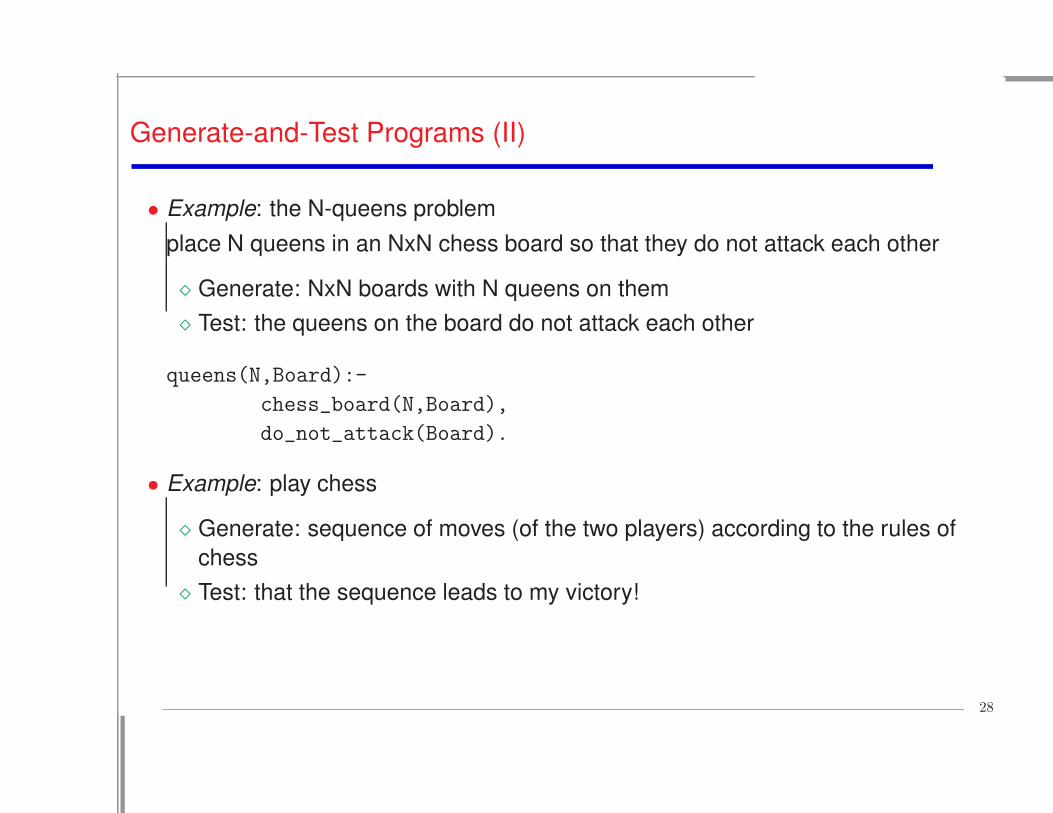
Generate-and-Test Programs (II)

• Example: the N-queens problem

place N queens in an NxN chess board so that they do not attack each other

⋄ Generate: NxN boards with N queens on them

⋄ Test: the queens on the board do not attack each other

queens(N,Board):-

chess_board(N,Board),

do_not_attack(Board).

• Example: play chess

⋄ Generate: sequence of moves (of the two players) according to the rules of

chess

⋄ Test: that the sequence leads to my victory!

28

Infinite Failure

• Generate-and-test may transform failure into infinite failure by generating infinite

possibilities none of which satisfy the test.

• Example: ?- reverse([1,2,3],[1,2,3| ]). with program:

reverse([],[]).

reverse([X|Xs],Ys) :-

append(Zs,[X],Ys),

reverse(Xs,Zs).

• It does not happen with program:

reverse([],[]).

reverse([X|Xs],Ys) :-

reverse(Xs,Zs),

append(Zs,[X],Ys).

• But it happens again now for query: ?- reverse([1,2,3| ],[1,2,3]).

29

Pruning Operator: Cut

• A “cut” (predicate !/0) commits Prolog to all the choices made since the parent

goal was unified with the head of the clause in which the cut appears.

• Thus, it prunes:

⋄ all clauses below the clause in which the cut appears, and

⋄ all alternative solutions to the goals in the clause to the left of the cut.

But it does not affect the search in the goals to the right of the cut.

s(a). p(X,Y):- l(X), ... r(a).

s(b). p(X,Y):- r(X), !, ... r(b).

p(X,Y):- m(X), ...

with query ?- s(A),p(B,C).

If execution reaches the cut (!):

⋄ The second alternative of r/1 is not considered.

⋄ The third clause of p/2 is not considered.

30

Pruning Operator: Cut (Contd.)

s(a). p(X,Y):- l(X), ... r(a).

s(b). p(X,Y):- r(X), !, ... r(b).

p(X,Y):- m(X), ...

p(B,C)

l(B)

B/a

!,...

l(B) m(B)

p(B,C)

A/bA/a

m(B)

B/b B/bB/a

r(B),!,...

| ?- s(A), p(B,C).

!,... !,...!,...

r(B),!,...

31

Types of Cut

• White cuts: do not discard solutions.

max(X,Y,X):- X > Y, !.

max(X,Y,Y):- X =< Y.

They affect neither completeness nor correctness – use them freely.

(In many cases the system “introduces” them automatically.)

• Green cuts: discard correct solutions which are not needed.

address(X,Add):- home_address(X,Add), !.

address(X,Add):- business_address(X,Add).

membercheck(X,[X|Xs]):- !.

membercheck(X,[Y|Xs]):- membercheck(X,Xs).

They affect completeness but not correctness.

Necessary in many situations (but beware!).

32

Types of Cut (Contd.)

• Red cuts: discard solutions which are not correct according to the intended

meaning.

⋄ Example:

max(X,Y,X):- X > Y, !.

max(X,Y,Y).

wrong answers to, e.g., ?- max(5, 2, 2).

⋄ Example:

days_in_year(X,366):- leap_year(X), !.

days_in_year(X,365).

wrong answers to, e.g., ?- days in year(a, D).

Red cuts affect completeness and one can no longer rely on the strict declarative

interpretation of the program for reasoning about correctness – avoid when

possible.

33

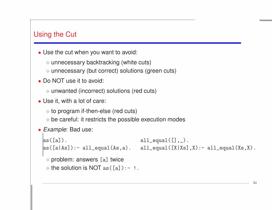
Using the Cut

• Use the cut when you want to avoid:

⋄ unnecessary backtracking (white cuts)

⋄ unnecessary (but correct) solutions (green cuts)

• Do NOT use it to avoid:

⋄ unwanted (incorrect) solutions (red cuts)

• Use it, with a lot of care:

⋄ to program if-then-else (red cuts)

⋄ be careful: it restricts the possible execution modes

• Example: Bad use:

as([a]). all_equal([],_).

as([a|As]):- all_equal(As,a). all_equal([X|Xs],X):- all_equal(Xs,X).

⋄ problem: answers [a] twice

⋄ the solution is NOT as([a]):- !.

34

Summary

• All that there is in logic programs is recursion and unification.

(And backtracking.)

• Terms allow you to define any data structure and unification to manipulate it.

• Recursion allows you to program other control structures (with some help).

• Backtracking gives you the possibility to program search.

• Ordering of clauses, ordering of goals, and the cut are the only means to control

execution.

• When designing programs, you can think of recursion in several ways.

35

Learning to Compose Recursive Programs

• By induction (as in the previous examples): elegant, but generally difficult – not

the way most people do it.

• By generalization: State first the base case(s), and then think about the general

recursive case(s).

• By construction (computationally): Think of recursion as a traversal that

constructs some result.

• Sometimes it helps to compose programs with a given use in mind (e.g., forwards

execution –”think computationally”), but then:

⋄ Make sure it is declaratively correct.

⋄ Consider also if alternative uses make declarative sense.

(take into account all the possible modes)

• Sometimes it helps to look at well-written examples and use the same “schemas”.

E.g., a list traversal.

36

Learning to Compose Recursive Programs (Coda)

• Global top-down design approach:

⋄ state the general problem

⋄ break it down into subproblems

⋄ solve the pieces

• To some extent it is a simple question of practice...

37