SIViPDOI 10.1007/s11760-009-0139-y

ORIGINAL PAPER

Wavelet shrinkage: unification of basic thresholding functionsand thresholds

Abdourrahmane M. Atto · Dominique Pastor ·Grégoire Mercier

Received: 4 March 2009 / Revised: 15 September 2009 / Accepted: 16 September 2009© Springer-Verlag London Limited 2009

Abstract This work addresses the unification of some basicfunctions and thresholds used in non-parametric estimationof signals by shrinkage in the wavelet domain. The softand hard thresholding functions are presented as degeneratesmooth sigmoid-based shrinkage functions. The shrinkageachieved by this new family of sigmoid-based functions isthen shown to be equivalent to a regularization of wave-let coefficients associated with a class of penalty functions.Some sigmoid-based penalty functions are calculated, andtheir properties are discussed. The unification also concernsthe universal and the minimax thresholds used to calibratestandard soft and hard thresholding functions: thesethresholds pertain to a wide class of thresholds, called thedetection thresholds. These thresholds depend on two param-eters describing the sparsity degree for the wavelet represen-tation of a signal. It is also shown that the non-degeneratesigmoid shrinkage adjusted with the new detection thresholdsis as performant as the best up-to-date parametric and com-putationally expensive method. This justifies the relevanceof sigmoid shrinkage for noise reduction in large databasesor large size images.

Keywords Non-parametric estimation · Wavelets ·Shrinkage function · Penalty function · Detection thresholds

A. M. Atto (B) · D. Pastor · G. MercierTELECOM Bretagne, Brest, Francee-mail: am.atto@telecom-bretagne.eu

D. Pastore-mail: dominique.pastor@telecom-bretagne.eu

G. Merciere-mail: gregoire.mercier@telecom-bretagne.eu

1 Introduction

The soft and hard shrinkage (thresholding) functions arebasic functions widely used for estimating a signal via pro-jection in the wavelet domain. The soft and hard shrinkages[1] involve forcing to zero the coefficients with amplitudeslower than the selected threshold, and preserving (hard) orshrinking (soft) any coefficient, with amplitude above thisthreshold, by a value that equals the threshold height. Thresh-old selection for calibrating soft and hard thresholding func-tions has also been addressed by Donoho and Johnstone [1].These authors proposed the use of the universal and minimaxthresholds: the estimation by soft or hard thresholding withany of these thresholds yields near-optimal risk in the sensethat, asymptotically, the estimator achieves within a factorof 2 log N of the ideal risk, which is the risk achieved withthe aid of an oracle (see Donoho and Johnstone’s paper forfurther details).

However, in practice, the hard and the soft WaveShrinkestimators present drawbacks such as an important variance,when using hard thresholding, or a large bias, when usingsoft thresholding [2]. Many suggestions have been made toimprove the performance of these WaveShrink estimators.Some of them relate to the choice of the threshold [3,4],and others address the choice of the shrinkage (parametricBayesian shrinkage: [5–10]; non-parametric shrinkage func-tions: [11–14]; among others).

The different contributions proposed in the literature andaiming at improving the denoising performance have resultedin a huge number of wavelet-based methods for image de-noising. In addition, there exist many ways to improve agiven method (using suitable wavelet transform, adding intra-interscale predictors, exploiting redundancy, combiningseveral methods, and so forth). Actually, the most efficientdenoising algorithms such as [8] and [13] combine several

123

SIViP

of these techniques (interscale predictors, Gaussian smooth-ing, and laborious parameterizations) and thus, they loosethe simplicity (single function with explicit close form) andthe portability (using different wavelet transforms withoutadditional computations) of basic shrinkage functions.

However, note that processing large size signals andimages requires computationally fast techniques and process-ing large databases requires portability of the method. Weare thus interested in efficient denoising by wavelet shrink-age when the shrinkage function has an explicit close form,without any additional a priori consideration such as inter-scale predictor.

In this respect, the present work revisits the concept ofshrinkage function by addressing the consequences of tworecent results: the Smooth Sigmoid-Based Shrinkage (SSBS)functions of [14] and the detection thresholds of [4].

The SSBS functions are smooth functions and they allowfor a flexible control of the shrinkage through parameters thatmodel the attenuation imposed to small, median, and largedata. This makes it possible to correct the main drawbacksof the soft and hard shrinkage functions. In contrast to the“sum of derivative of Gaussian” parameterization of [13], theSSBS functions are defined by an explicit close form so thatwe can first adapt their shape according to the noise level andthe expected denoising level; in addition, these functions canbe used for any wavelet transform (orthogonal, redundant,multi-wavelets, complex wavelets, among others) withoutadditional computation, which is not the case for the methodssuch as the SURELET of [13] and the BLS-GSM of [8].

The detection thresholds are synthesized by considering arisk function chosen to be the probability of error for decid-ing that a coefficient is significant or not. They depend ontwo parameters that can be used to bound the sparsity degreeof the wavelet representation [15]. These thresholds are opti-mal in the sense that, for a certain class of signals, includingsparse signals, they lead to the same upper bound for the prob-ability of error than the Bayes test with minimal probabilityof error among all possible tests [4]. It is shown below thatthe standard minimax and universal thresholds are detectionthresholds corresponding to different degrees of sparsity.

Summarizing, the present paper extends the results estab-lished in [14] by providing (1) the general description of theSSBS parameters, that is, the relation that allows for com-puting the SSBS attenuation degree with respect to the SSBSthreshold and the asymptotic attenuation parameters (thishas been addressed in [14] only for the case of vanishingasymptotic attenuation), (2) the penalty functions associatedwith the SSBS functions in a regularization problem, (3) thecombination between the SSBS functions and the detectionthresholds defined in [4], and (4) experimental results empha-sizing the relevance of SSBS functions, combined with detec-tion thresholds, in image denoising of synthetic and real noisydata.

The organization of the paper is as follows. Section 2briefly describes the SSBS functions and provides theirparameter interpretation. This section also highlights thatthe hard and soft thresholding functions can be seen as limitSSBS functions. Section 3 provides the characterization ofthe SSBS functions in a regularization problem by computingthe SSBS penalty functions. Section 4 addresses the proper-ties of the detection thresholds. This section also discusses theselection of appropriate detection thresholds with respect tothe wavelet decomposition properties of some signals suchas smooth and piecewise regular ones. Section 5 presentsexperimental tests aimed at assessing the denoising qualityachieved using the SSBS functions combined with detectionthresholds. Finally, Sect. 6 concludes this work.

2 Unification of basic thresholding functions

In what follows, we consider standard wavelet-based estima-tion procedures for discrete time signals with dyadic samplesizes, equally spaced and fixed sample points. We use thestandard model

ci = di + εi , i = 1, 2, . . . , N , (1)

where c = {ci }1≤i≤N is the orthonormal wavelet transformof a noisy observation, d = {di }1≤i≤N is a sparse vector rep-resenting the wavelet coefficients of the unknown determinis-tic signal and noise ε = {εi }1≤i≤N is such that therandom variables {εi }1≤i≤N are independent and identicallydistributed (iid), Gaussian, with null mean and variance σ 2.

In short, εiiid∼ N (0, σ 2) for i = 1, 2, . . . , N . Vector d

is supposed to be sparse, meaning that the wavelet basisconcentrates a large proportion of the energy of the sig-nal in a small number of coefficients with large amplitudes.This heuristic notion of sparsity ranges from strong to weaksparsity.

By strong sparsity, we mean that the energy of the signal is“almost entirely” contained in a small number of coefficientswith large amplitudes (see the example given in Fig. 1). Inthis case, almost all the coefficients described as “small” arein fact quasi-null or with very small amplitudes, and so, donot contain significant information on the signal. For thisreason, thresholding rules like hard or soft thresholding areproved to be the relevant strategies for estimating the signal(see [1]).

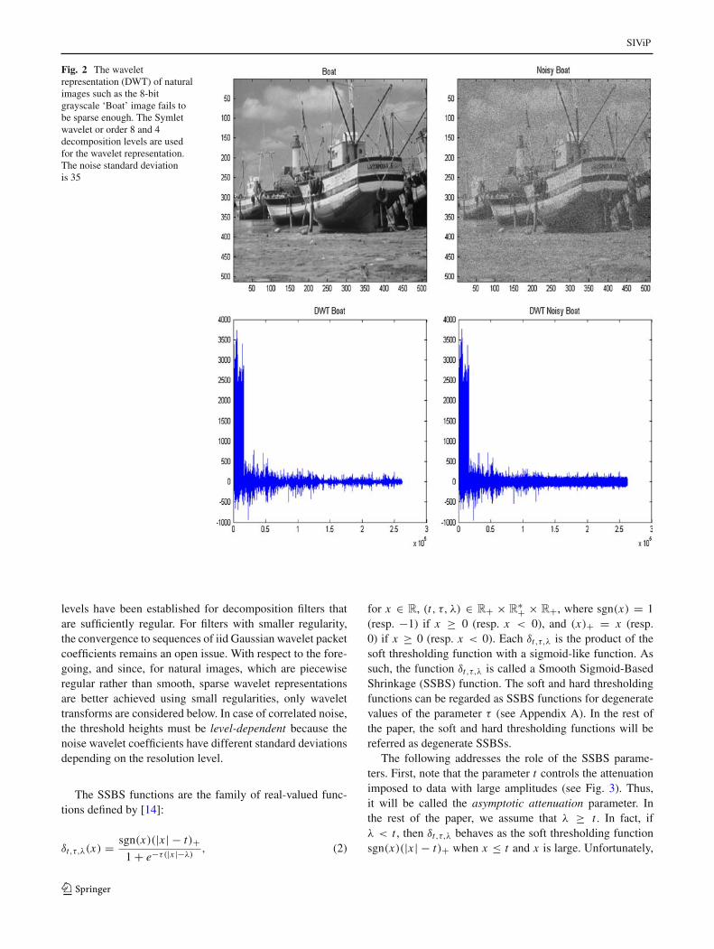
In the case of a representation which is not strongly sparse,it may often be useful to process small coefficients. In fact,wavelet representations of natural images fail to be sparseenough (see the example of Fig. 2): textures, contours arecharacterized by many small coefficients, and forcing all thesmall coefficients to zero may result in over-smoothing these

123

SIViP

Fig. 1 The discrete wavelettransform (DWT) of the ‘Cusp’signal is strongly sparse. Almostall the energies of the ‘Cusp’wavelet coefficients areconcentrated in a very fewnumber of large coefficients. Incontrast, the sparsity of thewavelet representation of the‘Blocks’ signal must beunderstood in the weak sense:this representation admits manysmall, but significantcoefficients, because thesecoefficients characterize thesingularities of the ‘Blocks’signal. The Symlet wavelet ororder 8 and 4 decompositionlevels are used for the waveletrepresentation

image characteristics and a loss of significant informationwhen the threshold height is large. Thus, in such a case ofweakly sparse representation, it may be preferable to con-sider, not a thresholding function, but a shrinkage functionthat performs a penalized shrinkage without systematicallyforcing to zero the small coefficients [14]. The family ofSmooth Sigmoid-Based Shrinkage (SSBS) functions (intro-duced in [14]) are shrinkage functions of that kind.

Remark 1 The model of Eq. (1) (in the wavelet domain)is justified when the input signal (in the temporal or spa-tial domain) is corrupted by Additive White Gaussian Noise(AWGN) and the wavelet transform used is orthonormal.In the case where additive noise is either coloured or notGaussian, this model remains approximately valid in the fol-lowing sense. The wavelet transform has interesting asymp-totic statistical properties. In fact, the coefficients returnedby the wavelet transform tend to be iid Gaussian when thedecomposition level is large enough for stationary random

processes [16–20] and some non-stationary randomprocesses such as fractional Brownian motions or fraction-ally differenced processes [21–25]. Thus, for a large classof random noises, one can expect that the wavelet coeffi-cients are quasi-decorrelated and approximately Gaussiandistributed for large resolution levels. Note that the aboveproperty might not be satisfied at the first resolution lev-els for strongly correlated processes and the wavelet coef-ficients may thus remain strongly correlated at resolutionlevels that are not large enough. In this case, a solutionwould be to use the coefficients, provided by a full wave-let packet decomposition, at large enough resolution levels.Indeed, the wavelet packet decomposition also returns coef-ficients that tend to be iid Gaussian at every node of suf-ficiently large resolution levels. However, the convergenceis more intricate than in the case of the wavelet transform,because the wavelet packet decomposition filters play animportant role in this convergence. In fact, the asymptoticdecorrelation and Gaussianity at large enough decomposition

123

SIViP

Fig. 2 The waveletrepresentation (DWT) of naturalimages such as the 8-bitgrayscale ‘Boat’ image fails tobe sparse enough. The Symletwavelet or order 8 and 4decomposition levels are usedfor the wavelet representation.The noise standard deviationis 35

levels have been established for decomposition filters thatare sufficiently regular. For filters with smaller regularity,the convergence to sequences of iid Gaussian wavelet packetcoefficients remains an open issue. With respect to the fore-going, and since, for natural images, which are piecewiseregular rather than smooth, sparse wavelet representationsare better achieved using small regularities, only wavelettransforms are considered below. In case of correlated noise,the threshold heights must be level-dependent because thenoise wavelet coefficients have different standard deviationsdepending on the resolution level.

The SSBS functions are the family of real-valued func-tions defined by [14]:

δt,τ,λ(x) = sgn(x)(|x | − t)+1 + e−τ(|x |−λ)

, (2)

for x ∈ R, (t, τ, λ) ∈ R+ × R

∗+ × R+, where sgn(x) = 1(resp. −1) if x ≥ 0 (resp. x < 0), and (x)+ = x (resp.0) if x ≥ 0 (resp. x < 0). Each δt,τ,λ is the product of thesoft thresholding function with a sigmoid-like function. Assuch, the function δt,τ,λ is called a Smooth Sigmoid-BasedShrinkage (SSBS) function. The soft and hard thresholdingfunctions can be regarded as SSBS functions for degeneratevalues of the parameter τ (see Appendix A). In the rest ofthe paper, the soft and hard thresholding functions will bereferred as degenerate SSBSs.

The following addresses the role of the SSBS parame-ters. First, note that the parameter t controls the attenuationimposed to data with large amplitudes (see Fig. 3). Thus,it will be called the asymptotic attenuation parameter. Inthe rest of the paper, we assume that λ ≥ t . In fact, ifλ < t , then δt,τ,λ behaves as the soft thresholding functionsgn(x)(|x | − t)+ when x ≤ t and x is large. Unfortunately,

123

SIViP

(a) (b)

Fig. 3 Graphs of δt,τ,λ for t = 0 (a δt,τ,λ: t = 0) and t �= 0 (b δt,τ,λ:t > 0). The dotted lines represent the values ±λ

soft thresholding is known to over-smooth the estimate whent is either the universal or the minimax threshold.

Second, the parameter λ will be described as the SSBSthreshold because it acts as a threshold. δ0,∞,λ is a hard thres-holding function with threshold height λ.

Finally, after a re-parameterization of the SSBS model (seeAppendix B), we obtain that τ can be written as a functionof t , θ and λ, where θ is an angle that relates to the curvatureof the SSBS arc in the interval (t, λ), that is, the attenua-tion we want to impose to data with in-between amplitudes.Since we have 0 < θ < arccos ((λ − t)/

√4λ2 + (λ − t)2),

the larger θ , the stronger the attenuation of the coefficientswith amplitudes in (t, λ). Hereafter, parameter θ will becalled the attenuation degree and the SSBS functions arewritten, equivalently, in the form δt,θ,λ, where the bijec-tion between (t, θ, λ) and (t, τ, λ) is detailed in Appendix B(see, in particular, Eqs. (25) and (26) in the saidappendix).

In practice, when t and λ are fixed, the foregoing makes itpossible to control the attenuation degree we want to imposeto the data in (t, λ) by choosing θ , a rather natural parameter.This interpretation of the SSBS parameters makes it easierto select convenient values of these parameters for practicalapplications. Summarizing, the estimation procedure is per-formed in three steps:

1. Fix the asymptotic attenuation t , the threshold λ and theattenuation degree θ of the SSBS function.

2. Compute the corresponding value of τ from Eq. (26).3. Shrink the data according to the SSBS function δt,τ,λ of

Eq. (2).

Some SSBS graphs are plotted in Fig. 4 for different val-ues of the attenuation degree θ (threshold λ is fixed and theasymptotic attenuation parameter t is 0).

Fig. 4 Shapes of SSBS functions δθ,λ for different values of theattenuation degree θ : θ = π/6 for the continuous (blue) curve, θ = π/4for the dotted (red) curve, and θ = π/3 for the dashed (magenta) curve

3 Penalty functions associated to SSBSin a regularization problem

Consider signal estimation using the penalized least squaresapproach given in [12]. In this reference, the signal estimationis addressed by considering a penalty function qλ = qλ(·) andby looking for the vector d that minimizes

||d − c||2�2+ 2

N∑

i=1

qλ(|di |). (3)

In [26], the unification between shrinkages and regulari-zation procedures is discussed. It follows from this referencethat shrinkages and regularization procedures are linked inthe sense that a shrinkage function corresponds to a regular-ization problem with a specific penalty function. This corre-spondence is made more precise by the following proposition:

Proposition 1 [26, Proposition 3.2]. Let δ be a real valuedthresholding function that is increasing, antisymmetric, suchthat 0 ≤ δ(x) ≤ x for x ≥ 0 and δ(x) tends to infinity asx tends to infinity. Then, there exists a continuous positivepenalty function q, with q(|x |) ≤ q(|y|) whenever |x | ≤ |y|,such that δ(z) is the unique solution of the minimization prob-lem mint (t−z)2+2q(|t |) for every z at which δ is continuous.The penalty q associated with δ is given by

q(x) =x∫

0

(r(z) − z)dz, (4)

for x ≥ 0, where r is the generalized inverse of δ:r(x) = sup{z | δ(z) ≤ x}.

An SSBS function δt,τ,λ satisfies the assumptions of Prop-osition 1. It follows that the shrinkage obtained using a func-tion δt,τ,λ can be seen as a regularization approximation witha continuous positive penalty function. The following char-acterizes the penalty function associated to δτ,λ = δ0,τ,λ.

123

SIViP

Proposition 2 The shrinkage obtained using an SSBSfunction δτ,λ can be seen as a regularization approximationwith penalty function qτ,λ, where qτ,λ is the function definedfor every x ≥ 0 by

qτ,λ(x) = 1

τ

x∫

0

L(τ ze−τ(z−λ)

)dz, (5)

with L being the Lambert function defined as the inverse ofthe function: t ≥ 0 �−→ tet .

Proof Since SSBS functions are continuous and strictlyincreasing functions, the generalized inverse of any SSBSfunction δτ,λ is the inverse, denoted rτ,λ, of this SSBS func-tion. From Proposition 1, the penalty associated with δτ,λ isthen

qτ,λ(x) =x∫

0

(rτ,λ(z) − z)dz. (6)

Now, because the SSBS function δτ,λ is continuous,strictly increasing and antisymmetric, its inverse rτ,λ has theform

rτ,λ(z) = zG(z), (7)

for every real value z and where G is such that

G(z) = 1 + e−τ(|z|G(z)−λ). (8)

Therefore, G(z) > 1 for any real value z. We thus have

(G(z) − 1) eτ(|z|(G(z)−1) = e−τ(|z|−λ), (9)

which is also equivalent to

τ |z| (G(z) − 1) eτ(|z|(G(z)−1) = τ |z|e−τ(|z|−λ). (10)

It follows that

τ |z| (G(z) − 1) = L(τ |z|e−τ(|z|−λ)

), (11)

which leads to

G(z) = 1 + L(τ |z|e−τ(|z|−λ)

)/(τ |z|) (12)

for z �= 0. Taking into account (7), (12) and the fact thatrτ,λ(0) = 0 since δτ,λ(0) = 0, we obtain

rτ,λ(z) = z + sgn(z)L(τ |z|e−τ(|z|−λ)

)/τ (13)

for any real value z. The result then follows by injectingEq. (13) into Eq. (6).

From Proposition 2, we derive that for every real value x ,the value δτ,λ(x) is the unique solution of the minimizationproblem mind((x − d)2 + 2qτ,λ(|d|)) where qτ,λ is givenby Eq. (5). The shape of the SSBS penalty qτ,λ(|x |) is givenfor fixed λ and several values of τ in Fig. 5; the penalties

Fig. 5 Penalty functions associated with the SSBS functions of Fig. 4in the regularization problem of Eq. (3). The attenuation degree θ is:θ = π/6 for the continuous (blue) curve, θ = π/4 for the dotted (red)curve, and θ = π/3 for the dashed (magenta) curve

displayed in this figure are those associated with the SSBSfunctions of Fig. 4.

It follows that the penalty associated with an SSBS func-tion is regular everywhere. This regularity depends on theSSBS shape. When the attenuation degree is small, the vari-ability of treatment among data is reduced, the shape of thepenalty function is more regular. In contrast, a large attenu-ation degree amplifies the variability of treatment, the slopeof the penalty shape is strong for small data and tends tobe quasi-null for large data (small data are strongly shrunkwhereas large data are approximately kept). Note, by compar-ing Fig. 5 with [26, Figure 3], the larger the SSBS attenuationdegree, the closer to the hard penalty the SSBS penalty is.

4 Unification of basic thresholds

In [4], it is shown that soft thresholding estimation of sig-nals in the wavelet domain can be improved using the detec-tion thresholds. In this section, we derive some propertiesof the detection thresholds proposed in [4]. In particular,Sect. 4.1 highlights that standard minimax and universalthresholds correspond to detection thresholds associated withdifferent sparsity degrees and Sect. 4.2 provides some detec-tion thresholds suitable for selecting the significant waveletcoefficients.

4.1 Detection thresholds

Consider the following decision problem with binary hypoth-esis model (H0,H1), where H0 : ci ∼ N (0, σ 2) versusH1 : ci = di + εi , |di | ≥ a > 0, εi ∼ N (0, σ 2).

Assume that the a priori probability of occurrence ofhypothesis H1 is less than or equal to some value p ≤ 1/2.Then, for deciding H0 versus H1, the thresholding test withthreshold height

λD(a, p) = σξ(a/σ, p), (14)

123

SIViP

where

ξ(a, p)= a

2+ 1

a

⎡

⎣ln1−p

p+ln

⎛

⎝1+√

1− p2

(1−p)2 e−a2

⎞

⎠

⎤

⎦ ,

(15)

has the same sharp upper bound for its probability of errorthan the Bayes test with the least probability of error (see [4]for details).

Parameter p reflects the presence (quantity) of signifi-cant coefficients of the signal among the noisy coefficients.Assuming that p is less than or equal to 1/2 ensures that therepresentation of the signal is, at least, sparse in the weaksense. Parameter a can be seen as the minimum amplitudeconsidered to be significant for a signal coefficient. Parame-ters p and a can thus be used to measure the sparsity degreeof the signal representation (see [4,15]).

The following proposition makes it possible to unify theminimax, universal, and detection thresholds.

Proposition 3 For any positive real value η ≥ σ , there exista0 > 0 and p0, with 0 ≤ p0 ≤ 1/2, such that

λD(a0, p0) = η. (16)

Proof The result simply follows by noting that the func-tion ξ is continuous, positive, lima→0 ξ(a, 1/2) = 1, andlima→+∞ ξ(a, p) = +∞ for any p such that 0 < p ≤ 1/2.

Let λu(N ) = σ

√2 ln N , the so-called universal thresh-

old. This threshold reflects the maximum amplitude of the

noise coefficients. Indeed, since εiiid∼ N (0, σ 2) for

i = 1, 2, . . . , N , then it follows from [27, p. 187] or[28, p. 454], that

limN→+∞ P

[λu(N ) − σ ln(ln N )

ln N≤ max {|εi |, 1 ≤ i ≤ N }

≤ λu(N )

]= 1. (17)

Thus, the maximum amplitude of {εi }1≤i≤N has a strongprobability of being close to the universal threshold when Nis large.

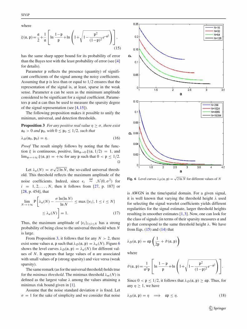
From Proposition 3, it follows that for any N > 2, thereexist some values a, p such that λD(a, p) = λu(N ). Figure 6shows the level curves λD(a, p) = λu(N ) for different val-ues of N . It appears that large values of a are associatedwith small values of p (strong sparsity) and vice versa (weaksparsity).

The same remark (as for the universal threshold) holds truefor the minimax threshold. The minimax threshold λm(N ) isdefined as the largest value λ among the values attaining aminimax risk bound given in [1].

Assume that the noise standard deviation σ is fixed. Letσ = 1 for the sake of simplicity and we consider that noise

Fig. 6 Level curves λD(a, p) = √2 ln N for different values of N

is AWGN in the time/spatial domain. For a given signal,it is well known that varying the threshold height λ usedfor selecting the signal wavelet coefficients yields differentregularities for the signal estimate, larger threshold heightsresulting in smoother estimates [1,3]. Now, one can look forthe class of signals (in terms of their sparsity measures a andp) that correspond to the same threshold height λ. We havefrom Eqs. (15) and (14) that

λD(a, p) = ap

(1

2p+ ϑ(a, p)

)

where

ϑ(a, p)= 1

a2p

⎡

⎣ln1 − p

p+ln

⎛

⎝1+√

1− p2

(1−p)2 e−a2

⎞

⎠

⎤

⎦.

Since 0 < p ≤ 1/2, it follows that λD(a, p) ≥ ap. Thus, forany η ≥ 1, we have

λD(a, p) = η ⇒ ap ≤ η. (18)

123

SIViP

Equation (18) confirms the fact that for a given value η

(threshold height), the “minimum significant amplitude forthe signal” a and the “proportion of significant signal coeffi-cients” p characterizing the surface λD(a, p) = η cannot beboth arbitrarily large because of the constraint ap ≤ η.

In addition, we have �(a, p) ≥ 1a2p

ln 1−pp and thus,

λD(a, p) ≥ 1a ln 1−p

p . By setting

p∗ = 1/ ln1 − p

p,

we have

λD(a, p) = η ⇒ ap∗ ≥ 1

η. (19)

Note that p∗ is a positive and strictly increasing function ofp (0 < p ≤ 1/2) and p∗ tends to 0 when p tends to 0. Thus,from Eq. (19), it follows that for any given threshold heightη ≥ 1, the “minimum significant amplitude for the signal” a

and the “proportion of significant signal coefficients” p char-acterizing the surface λD(a, p) = η cannot be both arbitrarilysmall because of the constraint ap∗ ≥ 1/η.

Summarizing, the class of signals (identified by the spar-sity measures a and p) that admit the same threshold heightis such that the uncertainty relations given by Eqs. (18) and(19) are satisfied. This class does not contain non-sparsesignals because both a and p cannot be arbitrary large orsmall (as a matter of justification, note that thresholding isnot very appropriate for estimating non-sparse signals). Thisclass contains sparse signals with different sparsity degrees:when a is large and p is small, we will say that the signalunder consideration admits a strongly sparse representation;in contrast, a weak sparse signal representation is such thata is small and p is large (with the upper-bound for p fixed tobe 1/2: p ≤ 1/2).

The above uncertainty relations thus allows for classifyingsignals according to their sparsity measures a and p and it fol-lows that strongly and weakly sparse signals have the samethreshold height η whenever their sparsity measures a and p

are such that λD(a, p) = η (see Fig. 6 for some examples oflevel curves such that λD(a, p) = η).

4.2 Detection thresholds adapted to the waveletdecomposition

Detection thresholds are well adapted to estimate waveletcoefficients corrupted by AWGN because of the sparsity ofthe wavelet transform [4]. Moreover, these thresholds areadaptable to the wavelet transform decomposition schemes:sparsity ensures that for reasonable resolution levels, signalcoefficients are less present than noise coefficients among thedetail wavelet coefficients and that signal coefficients havelarge amplitudes (in comparison to noise coefficients).

More precisely, it is known that for smooth or piecewiseregular signals, the proportion of significant coefficients,which plays a role similar to that of p, increases with theresolution level [28, Section 10.2.4, p. 460]. Therefore, ifwe can give, first, upper-bounds (p j ) j=1,2,...,J ; p j ≤ 1/2for every decomposition levels j = 1, 2, . . . , J , and second,lower-bounds (a j ) j=1,2,...,J for the amplitudes of the signifi-cant wavelet coefficients, then we can derive level-dependentdetection thresholds that can select significant wavelet coef-ficients at every resolution level. Since significant informa-tion tends to be absent among the first resolution level detailwavelet coefficients, it is reasonable to set a1 = σ

√2 ln N ,

that is the universal threshold. Now, when the resolution levelincreases, it follows from [28, Theorem 6.4] that a convenientchoice for a j , j > 1 is a j = a1/

√2 j−1 when the signal of

interest is smooth or piecewise regular.In addition, since noise tends to be less present when the

resolution level increases, p j must be an increasing functionof j . Note that detection thresholds are defined for p j ≤ 1/2.It is thus necessary to stop the shrinkage at a resolutionlevel J for which pJ is less than or equal to 1/2. We pro-pose the use of exponentially or geometrically increasingsequences for the values (p j ) j=1,2,...,J because p1 must be avery small value (significant information tends to be absentamong the first resolution level detail wavelet coefficients)and the presence of significant information increases signif-icantly as the resolution level increases. In the following, weconsider a sequence (p j ) j=1,2,...,J such that p j+1 = (p j )

1/µ

with µ > 1.Summarizing, we consider the thresholds λD(a j , p j ),

where λD is defined by Eq. (14) and (a j , p j ), forj = 1, 2, . . . , J are given by

a j = σ√

ln N/2 j/2−1, (20)

and

p j = 1/2µJ− j. (21)

5 SSBS and detection thresholds in practice

This section provides experimental results which highlightthat SSBS allows for noise reduction with preservation ofstructural details of images. We first discuss the calibrationof the SSBS parameters and assess the SSBS performancewhen noise is AWGN (Sect. 5.1). We then apply SSBS tothe denoising of SAR (Synthetic Aperture Radar) images(Sect. 5.2).

Experimental tests are carried out using the StationaryWavelet Transform (SWT) [29]. The maximum decomposi-tion level is fixed to J = 4. The SWT has appreciable proper-ties in denoising. Its redundancy makes it possible to reduce

123

SIViP

residual noise and some possible artefacts incurred by thetranslation sensitivity of the orthonormal wavelet transform.

5.1 Denoising images corrupted by synthetic AWGN

In this section, we consider a class of test images corruptedby synthetic AWGN. We use the PSNR and the StructuralSIMilarity (SSIM) index in order to assess the quality of adenoised image. The PSNR (peak signal-to-noise ratio, indeciBel unit, dB) refers to the mean square error (MSE) andis given by

PSNR = 10 log10

(2552/MSE

), (22)

The SSIM index [30] is a perceptual measure that comparespatterns of pixel intensities for images, on the basis of thelocal luminance and contrast of the analysed pixels. Let xand y be two data vectors assumed to contain non-negativevalues only and representing the pixel values to be compared.The luminance and the contrast of these pixels are estimatedby the mean and the standard deviation of x and y, respec-tively. The SSIM index between x and y is then given by [30]:

SSIM = (2µxµy + C1)(2σxy + C2)

(µ2x + µ2

y + C1)(σ 2x + σ 2

y + C2), (23)

where µx , σx (resp. µy , σy) are the mean and standard devia-tion of x (resp. y) and σxy designate the covariance betweenx and y. The local statistics µx , µy, σx , σy , and σxy arecomputed within a window with size 11 × 11 and the pixelvalues in this window are normalized using a unit sumcircular-symmetric Gaussian weighting function (see [30]for details). We also use the constants C1 and C2 suggestedby the authors in [30]: C1 = (K1L)2, C2 = (K2L)2 withK1 = 0.01 and K2 = 0.03, where L is the dynamic range ofthe pixel values (L = 255 for 8-bit grayscale images). TheSSIM index of two images is then the average value of thedifferent SSIM indices obtained by sliding the local windowover the entire image.

5.1.1 Preliminary tests

We first run some preliminary tests in order to choose theSSBS parameters and analyse the sensitivity of these parame-ters. We consider the standard ‘House’, ‘Barbara’, and ‘Lena’images, which are very popular in the image denoising com-munity. The tests are based on an analysis of the meansand variances of the PSNRs and SSIMs computed over 10noise realizations, when the test images are denoised by theSSBS method. The tested images are corrupted by AWGNwith standard deviation σ = 5, 10, 15, 20, 25, 30, 35 and theSWT is computed using different Daubechies, spline, andsymlet wavelet filters.

Given a fixed global threshold that can be either theuniversal threshold (λu), the minimax threshold (λm) or theuniversal-detection threshold (λud , obtained by settinga = σ

√2 ln N and p = 1/2 in Eq. (14), see [4] for the

properties of this threshold), the tests suggest using small(resp. large) asymptotic attenuation t and attenuation degreeθ when the noise level is small (resp. large). The same remarkholds for the level-dependent detection thresholds λD( j) =λD(a j , p j ) defined by Eq. (14), where (a j , p j ), for j =1, 2, . . . , J are given by Eqs. (20) and (21). The valueµ = 2.35 in Eq. (21) tends to be a good compromise for thedifferent test images used, when we assume that pJ = 1/2.

Among the global thresholds, the minimax and theuniversal-detection thresholds outperform the universalthreshold, and the universal-detection threshold tends to bemore performant than the minimax threshold, especiallywhen the noise level is not very large. The level-depen-dent thresholds perform better than the global thresholdsdescribed above when the noise standard deviation is largerthan 10. In addition, the preliminary tests show that reason-able asymptotic attenuation and attenuation degree parame-ters for SSBS are

• 0 ≤ t ≤ σ/10 and 0 < θ ≤ π/10 when the noise stan-dard deviation σ is less than 10,

• 0 ≤ t ≤ σ/5 and π/10 ≤ θ ≤ π/6 when 10 ≤ σ < 20,and

• σ/10 ≤ t ≤ σ/3 and π/6 ≤ θ ≤ π/4 when σ is largerthan or equal to 20.

For fixed parameters, we also test the sensitivity of theSSBS method according to the wavelet filters used. It fol-lows that, for a given wavelet family, there is no significantvariability of the results with respect to the length of thewavelet filter used. In addition, there is no significant dif-ference between the results obtained whatever the waveletfamily used, provided that the length of the filters remainapproximately of the same order.

5.1.2 SSBS denoising performance

In this section, we compare SSBS and BLS-GSM denoisingperformance. The BLS-GSM of [8] (free MatLab software1)is a parametric method using redundant wavelet transformand models neighbourhoods of wavelet coefficients withGaussian vectors multiplied by random positive scalars. BLS-GSM also takes into account the orientation and the interscaledependencies of the wavelet coefficients. It is actually thebest parametric method using redundant wavelet transform.

We present in Tables 1, 2, and 3, some experimental results(PSNRs and SSIMs performed by the SSBS) when the tested

1 Avalaible at http://decsai.ugr.es/~javier/denoise/software/index.htm.

123

SIViP

Table 1 Means of the PSNRs and SSIMs computed over 10 noise realizations, when denoising the ‘Boat’ image by the SSBS method (σ = 5)

t = 0 t = σ/10 t = σ/5

λm λud λD( j) λm λud λD( j) λm λud λD( j)

PSNRθ = π/14 36.16 36.53 36.28 36.01 36.48 36.14 35.84 36.38 35.99

θ = π/12 36.23 36.55 36.32 36.09 36.52 36.19 35.92 36.44 36.04

θ = π/10 36.25 36.54 36.30 36.12 36.52 36.16 35.96 36.45 36.03

θ = π/8 36.18 36.48 36.20 36.05 36.47 36.06 35.92 36.40 35.93

θ = π/6 35.94 36.30 35.87 35.82 36.28 35.75 35.68 36.24 35.64

SSIM

θ = π/14 0.928 0.933 0.930 0.926 0.932 0.928 0.923 0.931 0.926

θ = π/12 0.928 0.933 0.930 0.926 0.933 0.928 0.924 0.931 0.925

θ = π/10 0.928 0.934 0.929 0.926 0.933 0.926 0.923 0.931 0.924

θ = π/8 0.926 0.933 0.926 0.924 0.932 0.923 0.921 0.931 0.921

θ = π/6 0.921 0.930 0.919 0.918 0.929 0.916 0.915 0.928 0.913

The SSBS parameters (t, θ, λ) used are given in the table. The PSNR and the SSIM performed by the BLS-GSM method are 36.72 dB and 0.929,respectively

Table 2 Means of the PSNRs and SSIMs computed over 10 noise realizations, when denoising the ‘Boat’ image by the SSBS method (σ = 10)

t = 0 t = σ/10 t = σ/5

λm λud λD( j) λm λud λD( j) λm λud λD( j)

PSNRθ = π/14 32.25 32.38 32.55 32.20 32.45 32.52 32.10 32.47 32.46

θ = π/12 32.41 32.46 32.70 32.36 32.55 32.65 32.28 32.59 32.59

θ = π/10 32.58 32.55 32.84 32.51 32.65 32.78 32.42 32.69 32.70

θ = π/8 32.70 32.62 32.92 32.61 32.72 32.85 32.51 32.77 32.76

θ = π/6 32.66 32.63 32.84 32.55 32.72 32.76 32.44 32.76 32.64

SSIM

θ = π/14 0.851 0.849 0.860 0.853 0.853 0.861 0.853 0.856 0.861

θ = π/12 0.856 0.853 0.864 0.857 0.857 0.865 0.856 0.859 0.865

θ = π/10 0.861 0.857 0.869 0.861 0.861 0.869 0.860 0.863 0.868

θ = π/8 0.865 0.862 0.872 0.864 0.865 0.871 0.861 0.867 0.869

θ = π/6 0.864 0.865 0.870 0.861 0.867 0.867 0.857 0.868 0.864

The SSBS parameters (t, θ, λ) used are given in the table. The PSNR and the SSIM performed by the BLS-GSM method are 33.48 dB and 0.878,respectively

image is the ‘Boat’ image (the variances are very small incomparison with the mean PSNRs). The results are simi-lar with other standard images such as the ‘Peppers’ andthe ‘Fingerprint’ images. We focus on the case where thenoise standard deviation σ is between 5 and 15. Indeed,this case is of interest since when σ ≤ 3, noise is oftennon-perceptible and noise observed in images processed bymodern acquisition systems is often moderate. We run theSSBS denoising procedure described above. The SWT iscomputed using the biorthogonal spline wavelet with order3 for the decomposition and order 1 for the reconstruction(‘bior1.3’ in Matlab Wavelet toolbox). Several values forthe SSBS parameters are tested. These values are chosen

according to the recommendations made in the previous sec-tion. We also present in the captions of Tables 1, 2, and 3,the PSNRs and SSIMs achieved by the BLS-GSM methodof [8].

According to the experimental results presented inTables 1, 2, and 3, the performance of SSBS and BLS-GSMare of the same order, both in terms of PSNR and SSIM. TheBLS-GSM yields a PSNR slightly higher than the SSBS, thedifference in PSNR between SSBS and BLS-GSM being lessthan 1 dB. The (best) SSBS yields higher SSIM quality indexwhen the noise standard deviation is 5 and the BLS-GSMSSIM is slightly higher when the noise standard deviation is10, 15.

123

SIViP

Table 3 Means of the PSNRs and SSIMs computed over 10 noise realizations, when denoising the ‘Boat’ image by the SSBS method (σ = 15)

t = 0 t = σ/10 t = σ/5

λm λud λD( j) λm λud λD( j) λm λud λD( j)

PSNRθ = π/14 29.84 29.78 30.21 29.87 29.95 30.28 29.86 30.06 30.29

θ = π/12 30.08 29.94 30.43 30.09 30.11 30.49 30.08 30.24 30.48

θ = π/10 30.35 30.11 30.68 30.34 30.30 30.70 30.30 30.42 30.69

θ = π/8 30.60 30.31 30.91 30.57 30.48 30.89 30.50 30.60 30.85

θ = π/6 30.74 30.47 31.01 30.66 30.64 30.95 30.54 30.73 30.86

SSIM

θ = π/14 0.770 0.758 0.783 0.776 0.768 0.790 0.781 0.777 0.794

θ = π/12 0.781 0.766 0.794 0.786 0.776 0.800 0.790 0.785 0.803

θ = π/10 0.794 0.777 0.807 0.797 0.786 0.811 0.800 0.794 0.814

θ = π/8 0.808 0.789 0.821 0.809 0.798 0.822 0.809 0.805 0.822

θ = π/6 0.817 0.802 0.828 0.815 0.810 0.827 0.811 0.814 0.825

The SSBS parameters (t, θ, λ) used are given in the table. The PSNR and the SSIM performed by the BLS-GSM method are 31.63 dB and 0.839,respectively

From these results, it follows that SSBS and BLS-GSM arecomparable, both in terms of PSNR and SSIM quality index.In comparison with BLS-GSM, the advantage of SSBS isthen its extreme algorithmic simplicity. Indeed, SSBS canbe seen as a weighting function that simply applies to thewavelet coefficients, whereas BLS-GSM is computationallyexpensive and cannot be used in an operational context (see[13] for an appreciation of the BLS-GSM computing time).Note that, in contrast with the BLS-GSM and other denoisingmethods such as the SURELET of [13], which yields perfor-mances of the same order as BLS-GSM, SSBS uses neitherinterscale nor intrascale predictors. These predictors can beincluded in the shrinkage process for SSBS and they can cer-tainly allow for better denoising results. However, such pre-dictors are generally specific to the wavelet transform usedand, in this respect, they are detrimental to the portability ofa method. For this reason, we do not consider interscale andintrascale predictors in this paper. Also, note that SSBS mightbe adapted to other a priori knowledge using some directionalprocessing similar to that employed by BLS-GSM. However,when the noise level is small (which is the case of interest inpractical applications such as SAR denoising) then it follows,from the SSIM indices given in Table 1, that SSBS, withoutany additional a priori information, guarantees better preser-vation of structural information contained in the images thanBLS-GSM. In other words, SSBS guarantees noise reduc-tion without impacting significantly the signal characteristics(Figs. 7, 8, and 9 provide SSBS and BLS-GSM denoisingsfor the ‘Boat’ image as an illustration). In addition, it followsfrom Tables 1, 2, and 3 that SSBS denoising performance isnot really affected by slightly different SSBS parameter val-ues. This highlights the robustness of the method.

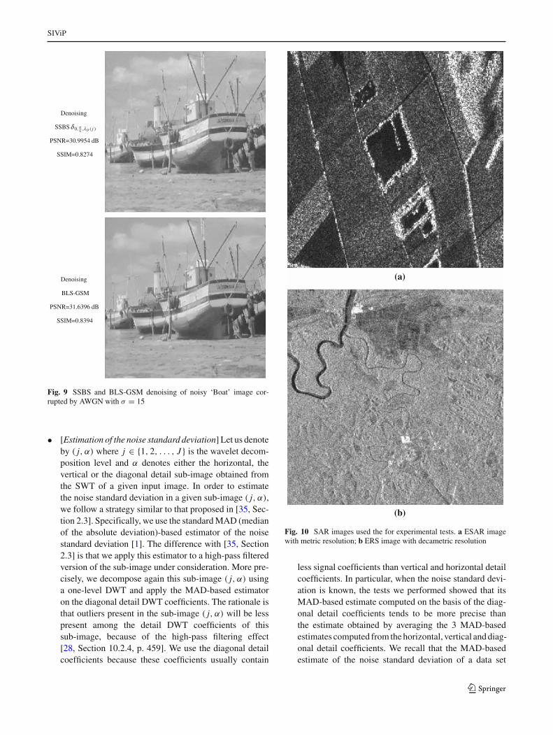
5.2 Denoising SAR images

In image processing, denoising is of interest, specifically forhigh-resolution images such as biomedical ultrasonic or SARimages, for instance. In such images, the signal reflectance zis corrupted by speckle noise ε. Speckle noise is modelled asa correlated stationary process, multiplicative with the sig-nal reflectance. The observation is then εz. We can writeεz = z + z(ε − 1) so as to consider that a SAR image is thesum of the signal reflectance z and a signal-dependent noisez(ε−1). In this signal-dependent noise case, the performanceof a wavelet shrinkage is not guaranteed to be as performantas in the AWGN case. Furthermore, we cannot guarantee thatthe signal-dependent noise wavelet coefficients can be ren-dered sufficiently iid Gaussian. However, for SAR images,speckle removal (despeckling) by wavelet shrinkage has beensuccessfully addressed by several authors, mostly in the caseof parametric models (see [31–33], among others). We thuscarry out some experiments on SAR images to assess therelevance of SSBS in this case.

According to Sect. 5.1.2, the advantage of SSBS in thecontext of SAR image despeckling is that SSBS is a sim-ple and performant non-parametric method that allows fordifferent levels of noise reduction, the noise reduction beingsmoothly adjustable thanks to the flexibility of the SSBSparameters. Because of this flexibility, we can investigatenoise reduction instead of full denoising for the SAR images.Indeed, because speckle contains much information, it mustnot be considered as pure noise. More precisely, we do notwish to fully remove speckle, but we want to reduce the vari-ability due to it, without impacting the structural informationof the SAR data.

123

SIViP

Noisy image

AWGN, σ = 5

PSNR=34.1514 dB

SSIM=0.8853

Noisy image

AWGN, σ = 15

PSNR=24.6090 dB

SSIM=0.5364

Fig. 7 Noisy ‘Boat’ image corrupted by AWGN with standarddeviation σ

• [Quality criterion] Since the reference (noise free) imageis not available, we use, as a quality criterion, the Equiv-alent Number of Looks (ENL) for the SAR images com-bined with the “method-noise” approach of [34]. TheENL of a SAR intensity image x is given by

ENL(x) = (Mean(x))2

Variance(x)

In an homogeneous region, and for a speckle free image,this quantity will often be very large since homogene-ity assumes small variability among the data. In contrast,in the presence of large variability among the data, thisquantity will often be small. When speckle is fully devel-oped in an homogeneous region of a SAR image, thenENL is a good estimate of the number of looks used toform the SAR intensity image.In addition, and since ENL does not make it possibleto measure the signal distortion caused by the denois-ing, we also use another quality criterion: a variant of the

Denoising

SSBSδ 0, π10 ,λ ud

PSNR=36.5719 dB

SSIM=0.9339

Denoising

BLS-GSM

PSNR=36.7129 dB

SSIM=0.9290

Fig. 8 SSBS and BLS-GSM denoising of noisy ‘Boat’ image cor-rupted by AWGN with σ = 5

‘method-noise’. The method-noise [34] simply involvesanalysing the difference between the original (noisy)image and the denoised image. According to this method,denoising quality is appreciated by checking the struc-tural contents of the method-noise (difference) image.Assuming that noise is additive, this method-noise imagelooks like a pure noise image for methods capable ofreducing noise without impacting the structural contentsof the images. In the case of SAR despeckling, weconsider the following variant of the method-noise. Thisvariant is hereafter called the ‘method-noise ratio’ andinvolves computing the ratio between the noisy imageand the denoised image. Indeed, the difference is lessinformative than the ratio because in the ideal case wherethe estimate equals the reflectance z, the difference con-sists of the signal-dependent noise z(ε − 1) whereas theratio is exactly the speckle noise ε. For the above variant,speckle reduction can be considered to be more accurate,that is, to better preserve the structural contents of thesignal reflectance, when the method-noise ratio imagelooks like pure speckle noise.

123

SIViP

Denoising

SSBSδ 0, π6 ,λD ( j )

PSNR=30.9954 dB

SSIM=0.8274

Denoising

BLS-GSM

PSNR=31.6396 dB

SSIM=0.8394

Fig. 9 SSBS and BLS-GSM denoising of noisy ‘Boat’ image cor-rupted by AWGN with σ = 15

• [Estimation of the noise standard deviation] Let us denoteby ( j, α) where j ∈ {1, 2, . . . , J } is the wavelet decom-position level and α denotes either the horizontal, thevertical or the diagonal detail sub-image obtained fromthe SWT of a given input image. In order to estimatethe noise standard deviation in a given sub-image ( j, α),we follow a strategy similar to that proposed in [35, Sec-tion 2.3]. Specifically, we use the standard MAD (medianof the absolute deviation)-based estimator of the noisestandard deviation [1]. The difference with [35, Section2.3] is that we apply this estimator to a high-pass filteredversion of the sub-image under consideration. More pre-cisely, we decompose again this sub-image ( j, α) usinga one-level DWT and apply the MAD-based estimatoron the diagonal detail DWT coefficients. The rationale isthat outliers present in the sub-image ( j, α) will be lesspresent among the detail DWT coefficients of thissub-image, because of the high-pass filtering effect[28, Section 10.2.4, p. 459]. We use the diagonal detailcoefficients because these coefficients usually contain

(a)

(b)

Fig. 10 SAR images used the for experimental tests. a ESAR imagewith metric resolution; b ERS image with decametric resolution

less signal coefficients than vertical and horizontal detailcoefficients. In particular, when the noise standard devi-ation is known, the tests we performed showed that itsMAD-based estimate computed on the basis of the diag-onal detail coefficients tends to be more precise thanthe estimate obtained by averaging the 3 MAD-basedestimates computed from the horizontal, vertical and diag-onal detail coefficients. We recall that the MAD-basedestimate of the noise standard deviation of a data set

123

SIViP

Table 4 ENLs obtained for SSBS denoising of the SAR images ofFig. 10

θ = π/8 θ = π/6

λm λud λD( j) λm λud λD( j)

SSBS ESAR image denoising

4.8164 4.0227 5.4051 4.6342 3.8766 5.3136

SSBS ERS image denoising

4.6397 3.6993 4.8125 4.4943 3.5570 4.7546

The SSBS parameter t is fixed to 0 for the denoising. The ENLs equal3.0729 for the original ESAR image and 2.6664 for the original ERSimage. The BLS-GSM denoising of these images yield ENLs equal3.9285 for the ESAR image and 13.4375 for the ERS image

x = (xi )i is given by σ = Median(|x |)/0.6745. Therobustness of the MAD is due to the fact that the medianis not really affected by a small number of outliers and isnot very sensitive to a small change in the data [1,36].

Figure 10 provides the SAR images used for the experi-mental tests. Table 4 presents the ENLs obtained by SSBSdenoising of these images (different SSBS parameters areused for the denoising). The ENLs are computed within awindow located in an homogeneous region for the imagesunder consideration (original images and denoised images).From Table 4, it follows that the variability reduction in theSAR data is more effective for SSBS adjusted with the level-dependent detection thresholds than for SBBS adjusted withthe minimax or the universal-detection threshold.

Examples of SAR SSBS denoisings are given in Figs. 11aand 12a. The SSBS parameters used are indicated below thefigure. The method-noise ratio images obtained from thesedenoisings are given in Figs. 13a and 14a. As can be seen inthese figures, the ratio between an original SAR image and itsSSBS denoised version looks like speckle noise; it does notcontain significant signal components. Thus, SSBS performsnoise reduction without significantly impacting the signalcharacteristics. The non-informative speckle components areremoved in homogenous areas whereas the speckle-like tex-tural information contained in the original data is preserved.Figures 11b, 12b, 13b, and 14b also provide experimentalresults for the BLS-GSM denoising of the SAR images ofFig. 10, for comparison with SSBS. The method-noise ratioimages obtained from the BLS-GSM denoising still containnon-speckled signal components, as can be seen in Figs. 13band 14b. The rough denoising performed by BLS-GSM (seeFigs. 11b and 12b) thus affects the structural information ofthe SAR data.

To conclude this section, note that a sub-class of SSBSfunctions constitutes a class of invertible functions. TheseSSBS functions are those obtained by setting t = 0. Forsuch an SSBS function, its inverse is given by Eq. (13). Thisallows for lossless denoising in the sense that one can retrieve

an original image from its denoised version by simply apply-ing the inverse denoising procedure: decompose the denoisedimage with the same wavelet transform as that initially used,apply the inverse of the SSBS function to the wavelet coef-ficients and reconstruct the original image using the inversewavelet transform. This lossless denoising might be rele-vant in many applications involving large databases. As amatter of fact, SAR, oceanography, and medical ultrasonicsensors record many gigabits of data per day. These data(images) are mainly corrupted by speckle noise. Losslessdespeckling of these databases is appealing since it is notessential to conserve a copy of the original database (thou-sands and thousands of gigabits recorded every year). UsingSSBS denoising, one can thus retrieve an original image(when needed) by simply applying the inverse denoising pro-cedure, which involves the inverse function of the SSBS usedfor the denoising.

6 Conclusion

Some noticeable properties of the SSBS functions and thedetection thresholds have been highlighted. The SSBSfunctions are a family of smooth sigmoid-based shrinkagefunctions that perform a penalized shrinkage. The standardhard and soft thresholding functions can be seen as degen-erate SSBS functions. The properties of the SSBS func-tions have been addressed on the basis of the geometricalinterpretation of their parameters. It follows that the SSBSfunctions are parameterized by 3 parameters that allow forcontrolling the attenuation degrees to be applied to small,median, and large values, the shrinkage process being regularsince non-degenerate SSBS functions are smooth functions.

On the other hand, this paper has also analysed the proper-ties of the detection thresholds. Detection thresholds dependon two parameters that describe the sparsity of the wave-let representation in terms of “minimum significant ampli-tude” for the signal and “probability of occurrence” of thesignificant signal coefficients in the sequence of the wave-let coefficients. It is shown that the universal and minimaxthresholds are particular detection thresholds correspondingto different degrees of sparsity.

Finally, the use of detection thresholds for calibratingSSBS functions has been addressed. We have selected theSSBS detection thresholds on the basis of the known behav-iour of the wavelet coefficients for smooth and piecewise reg-ular signals. The resulting shrinkage is performant for manyimages, including SAR images. The experimental resultsshow that SSBS functions adjusted with these detectionthresholds achieve denoising PSNRs and SSIMs comparableto those attained with the best parametric and computationally expensive method, the BLS-GSM of [8]. Thisperformance is remarkable for a non-parametric method

123

SIViP

(a)

(b)

Fig. 11 SSBS and BLS-GSM denoisings for the ESAR image ofFig. 10a. a ESAR image denoising using SSBS δ0, π

8 ,λD( j), b ESARimage denoising using BLS-GSM

where no interscale or intrascale predictors are used to pro-vide information about significant wavelet coefficients. TheSSBS functions are thus suitable functions for noise reduc-tion of large size signals and images. They also allow for alossless denoising (due to the invertibility of a sub-class ofSSBS functions), which can be relevant in many applicationsinvolving large databases.

An extension to this work could concern the estimationof the detection thresholds parameters a and p on the basisof the input noisy signal wavelet coefficients. This extension

(a)

(b)

Fig. 12 SSBS and BLS-GSM denoisings for the ERS image ofFig. 10b. a ESAR image, © ESA denoising using SSBS δ0, π

8 ,λD( j),b ESAR image, © ESA denoising using BLS-GSM

involves estimating the minimum significant wavelet coef-ficient for the signal and an upper bound on the probabilityof occurrence of significant wavelet coefficients. Combiningthis extension with predictors for detecting significant (small)wavelet coefficients could probably improve the SSBS per-formance.

Acknowledgments The authors are very grateful to the reviewers fortheir insightful comments. They also would like to thank E. Pottier andJ.P. Rudant for providing ESAR and ERS image data.

123

SIViP

(a)

(b)

Fig. 13 Image (a) is the ratio between the image of Fig. 10a and theimage of Fig. 11a. Image (b) is the ratio between the image of Fig. 10aand the image of Fig. 11b. a ESAR image method-noise ratio with SSBSδ0, π

8 ,λD( j), b ESAR image method-noise ratio with BLS-GSM

Appendix A: The soft and hard thresholding functionsare degenerate SSBS functions

For fixed t and λ, and if T = max (t, λ), then the functionδt,τ,λ(x) tends to the soft thresholding function sgn(x)(|x |−T )+ when τ tends to +∞.

Now, when τ tends to infinity, δ0,τ,λ(x) tends to δ0,∞,λ(x),which is a hard thresholding function defined by:

(a)

(b)

Fig. 14 Image (a) is the ratio between the image of Fig. 10b and theimage of Fig. 12a. Image (b) is the ratio between the image of Fig. 10band the image of Fig. 12b. a ESAR image, © ESA method-noise ratiowith SSBS δ0, π

8 ,λD( j), b ESAR image, © ESA method-noise ratio withBLS-GSM

δ0,∞,λ(x) ={

x1{|x |>λ} if x ∈ R \ {−λ, λ},±λ/2 if x = ±λ,

(24)

where 1� is the indicator function of a given set � ⊂ R:1�(x) = 1 if x ∈ �; 1�(x) = 0 if x ∈ R \ �. Notethat δ0,∞,λ sets a coefficient with amplitude λ to half of itsvalue and so, minimizes the local variation around λ, sincelimx→λ+ δ0,∞,λ(x)− 2δ0,∞,λ(λ)+ limx→λ− δ0,∞,λ(x) = 0.

123

SIViP

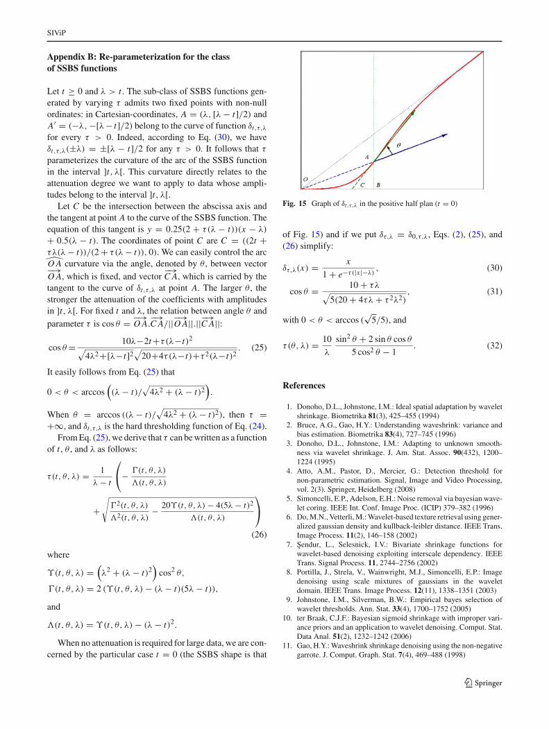
Appendix B: Re-parameterization for the classof SSBS functions

Let t ≥ 0 and λ > t . The sub-class of SSBS functions gen-erated by varying τ admits two fixed points with non-nullordinates: in Cartesian-coordinates, A = (λ, [λ − t]/2) andA′ = (−λ,−[λ− t]/2) belong to the curve of function δt,τ,λ

for every τ > 0. Indeed, according to Eq. (30), we haveδt,τ,λ(±λ) = ±[λ − t]/2 for any τ > 0. It follows that τ

parameterizes the curvature of the arc of the SSBS functionin the interval ]t, λ[. This curvature directly relates to theattenuation degree we want to apply to data whose ampli-tudes belong to the interval ]t, λ[.

Let C be the intersection between the abscissa axis andthe tangent at point A to the curve of the SSBS function. Theequation of this tangent is y = 0.25(2 + τ(λ − t))(x − λ)

+ 0.5(λ − t). The coordinates of point C are C = ((2t +τλ(λ − t))/(2 + τ(λ − t)), 0). We can easily control the arcO A curvature via the angle, denoted by θ , between vector−→O A, which is fixed, and vector

−→C A, which is carried by the

tangent to the curve of δt,τ,λ at point A. The larger θ , thestronger the attenuation of the coefficients with amplitudesin ]t, λ[. For fixed t and λ, the relation between angle θ andparameter τ is cos θ = −→

O A.−→C A/||−→O A||.||−→C A||:

cos θ = 10λ−2t+τ(λ−t)2√

4λ2+[λ−t]2√

20+4τ(λ−t)+τ 2(λ−t)2. (25)

It easily follows from Eq. (25) that

0 < θ < arccos((λ − t)/

√4λ2 + (λ − t)2

).

When θ = arccos ((λ − t)/√

4λ2 + (λ − t)2), then τ =+∞, and δt,τ,λ is the hard thresholding function of Eq. (24).

From Eq. (25), we derive that τ can be written as a functionof t , θ , and λ as follows:

τ(t, θ, λ) = 1

λ − t

⎛

⎝− �(t, θ, λ)

�(t, θ, λ)

+√

�2(t, θ, λ)

�2(t, θ, λ)− 20ϒ(t, θ, λ) − 4(5λ − t)2

�(t, θ, λ)

⎞

⎠

(26)

where

ϒ(t, θ, λ) =(λ2 + (λ − t)2

)cos2 θ,

�(t, θ, λ) = 2 (ϒ(t, θ, λ) − (λ − t)(5λ − t)),

and

�(t, θ, λ) = ϒ(t, θ, λ) − (λ − t)2.

When no attenuation is required for large data, we are con-cerned by the particular case t = 0 (the SSBS shape is that

Fig. 15 Graph of δt,τ,λ in the positive half plan (t = 0)

of Fig. 15) and if we put δτ,λ = δ0,τ,λ, Eqs. (2), (25), and(26) simplify:

δτ,λ(x) = x

1 + e−τ(|x |−λ), (30)

cos θ = 10 + τλ√

5(20 + 4τλ + τ 2λ2), (31)

with 0 < θ < arccos (√

5/5), and

τ(θ, λ) = 10

λ

sin2 θ + 2 sin θ cos θ

5 cos2 θ − 1. (32)

References

1. Donoho, D.L., Johnstone, I.M.: Ideal spatial adaptation by waveletshrinkage. Biometrika 81(3), 425–455 (1994)

2. Bruce, A.G., Gao, H.Y.: Understanding waveshrink: variance andbias estimation. Biometrika 83(4), 727–745 (1996)

3. Donoho, D.L., Johnstone, I.M.: Adapting to unknown smooth-ness via wavelet shrinkage. J. Am. Stat. Assoc. 90(432), 1200–1224 (1995)

4. Atto, A.M., Pastor, D., Mercier, G.: Detection threshold fornon-parametric estimation. Signal, Image and Video Processing,vol. 2(3). Springer, Heidelberg (2008)

5. Simoncelli, E.P., Adelson, E.H.: Noise removal via bayesian wave-let coring. IEEE Int. Conf. Image Proc. (ICIP) 379–382 (1996)

6. Do, M.N., Vetterli, M.: Wavelet-based texture retrieval using gener-alized gaussian density and kullback-leibler distance. IEEE Trans.Image Process. 11(2), 146–158 (2002)

7. Sendur, L., Selesnick, I.V.: Bivariate shrinkage functions forwavelet-based denoising exploiting interscale dependency. IEEETrans. Signal Process. 11, 2744–2756 (2002)

8. Portilla, J., Strela, V., Wainwright, M.J., Simoncelli, E.P.: Imagedenoising using scale mixtures of gaussians in the waveletdomain. IEEE Trans. Image Process. 12(11), 1338–1351 (2003)

9. Johnstone, I.M., Silverman, B.W.: Empirical bayes selection ofwavelet thresholds. Ann. Stat. 33(4), 1700–1752 (2005)

10. ter Braak, C.J.F.: Bayesian sigmoid shrinkage with improper vari-ance priors and an application to wavelet denoising. Comput. Stat.Data Anal. 51(2), 1232–1242 (2006)

11. Gao, H.Y.: Waveshrink shrinkage denoising using the non-negativegarrote. J. Comput. Graph. Stat. 7(4), 469–488 (1998)

123

SIViP

12. Antoniadis, A., Fan, J.: Regularization of wavelet approximations.J. Am. Stat. Assoc. 96(455), 939–955 (2001)

13. Luisier, F., Blu, T., Unser, M.: A new sure approach to imagedenoising: interscale orthonormal wavelet thresholding. IEEETrans. Image Process. 16(3), 593–606 (2007)

14. Atto, A.M., Pastor, D., Mercier, G.: Smooth sigmoid wave-let shrinkage for non-parametric estimation. IEEE InternationalConference on Acoustics, Speech, and Signal Processing, ICASSP,Las Vegas, Nevada, USA, 30 March–4 April (2008)

15. Pastor, D., Atto, A.M.: Sparsity from binary hypothesis testing andapplication to non-parametric estimation. European Signal Pro-cessing Conference, EUSIPCO, Lausanne, Switzerland, August25–29 (2008)

16. Benedetto, J.J., Frasier, M.W.: Wavelets : Mathematics and applica-tions. CRC Press, Boca Raton (1994), chap. 9: Wavelets, probabil-ity, and statistics: Some bridges, by Christian Houdré, pp. 365–398

17. Zhang, J., Walter, G.: A wavelet-based KL-like expansion forwide-sense stationary random processes. IEEE Trans. Signal Pro-cess. 42(7), 1737–1745 (1994)

18. Leporini, D., Pesquet, J.-C.: High-order wavelet packets and cumu-lant field analysis. IEEE Trans. Inf. Theory 45(3), 863–877 (1999)

19. Atto, A.M., Pastor, D., Isar, A.: On the statistical decorrelation ofthe wavelet packet coefficients of a band-limited wide-sense sta-tionary random process. Signal Process. 87(10), 2320–2335 (2007)

20. Atto, A.M., Pastor, D.: Limit distributions for wavelet packet coef-ficients of band-limited stationary random processes. EuropeanSignal Processing Conference, EUSIPCO, Lausanne, Switzerland,25–28 August (2008)

21. Flandrin, P.: Wavelet analysis and synthesis of fractional brownianmotion. IEEE Trans. Inf. Theory 38(2), 910–917 (1992)

22. Tewfik, A.H., Kim, M.: Correlation structure of the discrete wave-let coefficients of fractional brownian motion. IEEE Trans. Inf.Theory 38(2), 904–909 (1992)

23. Dijkerman, R.W., Mazumdar, R.R.: On the correlation structureof the wavelet coefficients of fractional brownian motion. IEEETrans. Inf. Theory 40(5), 1609–1612 (1994)

24. Kato, T., Masry, E.: On the spectral density of the wavelet trans-form of fractional brownian motion. J. Time Ser. Anal. 20(50), 559–563 (1999)

25. Craigmile, P.F., Percival, D.B.: Asymptotic decorrelation ofbetween-scale wavelet coefficients. IEEE Trans. Inf. Theory 51(3),1039–1048 (2005)

26. Antoniadis, A.: Wavelet methods in statistics: some recent devel-opments and their applications. Stat. Surveys 1, 16–55 (2007)

27. Berman, S.M.: Sojourns and Extremes of Stochastic Processes.Wadsworth and Brooks/Cole, USA (1992)

28. Mallat, S.: A Wavelet Tour of Signal Processing, 2nd edn. Aca-demic Press, New York (1999)

29. Coifman, R.R., Donoho, D.L.: Translation invariant de-noising.Lect. Notes Stat. (103), 125–150 (1995)

30. Wang, Z., Bovik, A.C., Sheikh, H.R., Simoncelli, E.P.: Image qual-ity assessment: from error visibility to structural similarity. IEEETrans. Image Process. 13(4), 600–612 (2004)

31. Sveinsson, J.R., Benediktsson, J.A.: Speckle reduction andenhancement of sar images in the wavelet domain. Geosci. RemoteSens. Symp. IGARSS 1, 63–66 (1996)

32. Xie, H., Pierce, L.E., Ulaby, F.T.: Sar speckle reduction using wave-let denoising and markov random field modeling. IEEE Trans. Geo-sci. Remote Sens. 40(10), 2196–2212 (2002)

33. Argenti, F., Bianchi, T., Alparone, L.: Multiresolution mapdespeckling of sar images based on locally adaptive generalizedgaussian pdf modeling. IEEE Trans. Image Process. 15(11), 3385–3399 (2006)

34. Buades, A., Coll, B., Morel, J.M.: A review of image denoisingalgorithms, with a new one. Multiscale Model. Simul. 4(2), 490–530 (2005)

35. Johnstone, I.M., Silverman, B.W.: Wavelet threshold estimators fordata with correlated noise. J. Royal Stat. Soc. Ser. B 59(2), 319–351(1997)

36. Müller, J.W.: Possible advantages of a robust evaluation of com-parisons. J. Res. Natl. Inst. Stand. Technol. 105(4), 551–555 (2000)

123