Extension and Unification of SingularPerturbation Methods for ODEs Based on the

Renormalization Group MethodDepartment of Applied Mathematics and Physics

Kyoto University, Kyoto, 606-8501, Japan

Hayato CHIBA *1

September 29, 2008; Revised May 1 2009

Abstract

The renormalization group (RG) method is one of the singular perturbation methods which

is used in search for asymptotic behavior of solutions of differential equations. In this arti-

cle, time-independent vector fields and time (almost) periodic vector fields are considered.

Theorems on error estimates for approximate solutions, existence of approximate invariant

manifolds and their stability, inheritance of symmetries from those for the original equation

to those for the RG equation, are proved. Further it is proved that the RG method unifies

traditional singular perturbation methods, such as the averaging method, the multiple time

scale method, the (hyper-) normal forms theory, the center manifold reduction, the geometric

singular perturbation method and the phase reduction. A necessary and sufficient condition

for the convergence of the infinite order RG equation is also investigated.

1 Introduction

Differential equations form a fundamental topic in mathematics and its application to nat-

ural sciences. In particular, perturbation methods occupy an important place in the theory of

differential equations. Although most of the differential equations can not be solved exactly,

some of them are close to solvable problems in some sense, so that perturbation methods,

which provide techniques to handle such class of problems, have been long studied.

This article deals with a system of ordinary differential equations (ODEs) on a manifold M

of the formdxdt= εg(t, x, ε), x ∈ M, (1.1)

which is almost periodic in t with appropriate assumptions (see the assumption (A) in

*1 E mail address : chiba@amp.i.kyoto-u.ac.jp

1

Sec.2.1), where ε ∈ R or C is a small parameter.

Since ε is small, it is natural to try to construct a solution of this system as a power series

in ε of the formx = x(t) = x0(t) + εx1(t) + ε2x2(t) + · · · . (1.2)

Substituting Eq.(1.2) into Eq.(1.1) yields a system of ODEs on x0, x1, x2, · · · . The method to

construct x(t) in this manner is called the regular perturbation method.

It is known that if the function g(t, x, ε) is analytic in ε, the series (1.2) converges to an exact

solution of (1.1), while if it is not analytic, (1.2) diverges and no longer provides an exact

solution. However, the problem arising immediately is that one can not calculate infinite

series like (1.2) in general whether it converges or not, because it involves infinitely many

ODEs on x0, x1, x2, · · · . If the series is truncated at a finite-order term in ε, another problem

arises. For example, suppose that Eq.(1.1) admits an exact solution x(t) = sin(εt), and that

we do not know the exact solution. In this case, the regular perturbation method provides a

series of the form

x(t) = εt − 13!

(εt)3 +15!

(εt)5 + · · · . (1.3)

If truncated, the series becomes a polynomial in t, which diverges as t → ∞ although the

exact solution is periodic in t. Thus, the perturbation method fails to predict qualitative prop-

erties of the exact solution. Methods which handle such a difficulty and provide acceptable

approximate solutions are called singular perturbation methods. Many singular perturbation

methods have been proposed so far [1,3,6,38,39,43,44,47,50] and many authors reported that

some of them produced the same results though procedures to construct approximate solu-

tions were different from one another [9,38,43,44,47].

The renormalization group (RG) method is the relatively new method proposed by Chen,

Goldenfeld and Oono [8,9], which reduces a problem to a more simple equation called the

RG equation, based on an idea of the renormalization group in quantum field theory. In

their papers, it is shown (without a proof) that the RG method unifies conventional singular

perturbation methods such as the multiple time scale method, the boundary layer technique,

the WKB analysis and so on.

After their works, many studies of the RG method have been done [10-13,16,21,22,26-

32,35,36,42,45,46,48,49,53,55-59]. Kunihiro [28,29] interpreted an approximate solution

obtained by the RG method as the envelope of a family of regular perturbation solutions.

Nozaki et al. [45,46] proposed the proto-RG method to derive the RG equation effectively.

Ziane [53] , DeVille et al. [32] and Chiba [10] gave error estimates for approximate solutions.

2

Chiba [10] defined the higher order RG equation and the RG transformation to improve error

estimates. He also proved that the RG method could provide approximate vector fields and

approximate invariant manifolds as well as approximate solutions. Ei, Fujii and Kunihiro

[16] applied the RG method to obtain approximate center manifolds and their method was

rigorously formulated by Chiba [12]. DeVille et al. [32] showed that lower order RG equa-

tions are equivalent to normal forms of vector fields, and this fact was extended to higher

order RG equations by Chiba [11]. Applications to partial differential equations are appeared

in [16,31,42,45,46,55-59].

One of the purposes of this paper is to give basic theorems on the RG method extending

author’s previous works [10-12], in which the RG method is discussed for more restricted

problems than Eq.(1.1). At first, definitions of the higher order RG equations for Eq.(1.1)

are given and properties of them are investigated. It is proved that the RG method provides

approximate vector fields (Thm.2.5) and approximate solutions (Thm.2.7) along with error

estimates. Further, it is shown that if the RG equation has a normally hyperbolic invariant

manifold N, the original equation (1.1) also has an invariant manifold Nε which is diffeomor-

phic to N (Thms.2.9, 2.14). The RG equation proves to have the same symmetries (action of

Lie groups) as those for the original equation (Thm.2.12). In addition, if the original equa-

tion is an autonomous system, the RG equation is shown to have an additional symmetry

(Thm.2.15). These facts imply that the RG equation is easier to analyze than the original

equation. An illustrative example to verify these theorems is also given (Sec.2.5).

The other purpose of this paper is to show that the RG method extends and unifies other tra-

ditional singular perturbation methods, such as the averaging method (Sec.4.1), the multiple

time scale method (Sec.4.2), the (hyper-) normal forms theory (Sec.4.3), the center manifold

reduction (Sec.3.2), the geometric singular perturbation method (Sec.3.3), the phase reduc-

tion (Sec.3.4), and Kunihiro’s method [28,29] based on envelopes (Sec.4.4). A few of these

results were partially obtained by many authors [9,38,43,44,47]. The present arguments will

greatly reveal the relations among these methods.

Some properties of the infinite order RG equation are also investigated. It is proved that

the infinite order RG equation converges if and only if the original equation is invariant under

an appropriate torus action (Thm.5.1). This result extends Zung’s theorem [54] which gives a

necessary and sufficient condition for the convergence of normal forms of infinite order. The

infinite RG equation for a time-dependent linear system proves to be convergent (Thm.5.6)

and be related to monodromy matrices in Floquet theory.

3

Throughout this paper, solutions of differential equations are supposed to be defined for all

t ∈ R.

2 Renormalization group method

In this section, we give the definition of the RG (renormalization group) equation and main

theorems on the RG method, such as the existence of invariant manifolds and inheritance

of symmetries. An illustrative example and comments on symbolic computation of the RG

equation are also provided.

2.1 Setting, definitions and basic lemmas

Let M be an n dimensional manifold and U an open set in M whose closure U is compact.

Let g(t, ·, ε) be a vector field on U parameterized by t ∈ R and ε ∈ C. We consider the system

of differential equationsdxdt= x = εg(t, x, ε). (2.1)

For this system, we make the following assumption.

(A) The vector field g(t, x, ε) is C1 with respect to time t ∈ R and C∞ with respect to x ∈ U

and ε ∈ E, where E ⊂ C is a small neighborhood of the origin. Further, g is an almost periodic

function with respect to t uniformly in x ∈ U and ε ∈ E, the set of whose Fourier exponents

has no accumulation points on R.

In general, a function h(t, x) is called almost periodic with respect to t uniformly in x ∈ U

if the set

T (h, δ) := {τ | ||h(t + τ, x) − h(t, x)|| < δ, ∀t ∈ R, ∀x ∈ U} ⊂ R

is relatively dense for any δ > 0; that is, there exists a positive number L such that [a, a+ L]∩T (h, δ) � ∅ for all a ∈ R. It is known that an almost periodic function is expanded in a Fourier

series as h(t, x) ∼ ∑an(x)eiλnt, (i =

√−1), where λn ∈ R is called a Fourier exponent. See

Fink [20] for basic facts on almost periodic functions. The condition for Fourier exponents in

the above assumption (A) is essentially used to prove Lemma 2.1 below. We denote Mod(h)

the smallest additive group of real numbers that contains the Fourier exponents λn of an

almost periodic function h(t) and call it the module of h.

4

Let∑∞

k=1 εkgk(t, x) be the formal Taylor expansion of εg(t, x, ε) in ε :

x = εg1(t, x) + ε2g2(t, x) + · · · . (2.2)

By the assumption (A), we can show that gi(t, x) (i = 1, 2, · · · ) are almost periodic functions

with respect to t ∈ R uniformly in x ∈ U such that Mod(gi) ⊂ Mod(g).

Though Eq.(2.1) is mainly considered in this paper, we note here that Eqs.(2.3) and (2.5)

below are reduced to Eq.(2.1): Consider the system of the form

x = f (t, x) + εg(t, x, ε), (2.3)

where f (t, ·) is a C∞ vector field on U and g satisfies the assumption (A). Let ϕt be the flow

of f ; that is, ϕt(x0) is a solution of the equation x = f (t, x) whose initial value is x0 at the

initial time t = 0. For this system, changing the coordinates by x = ϕt(X) provides

X = ε

(∂ϕt

∂X(X)

)−1

g(t, ϕt(X), ε) := εg(t, X, ε). (2.4)

We suppose that

(B) the vector field g satisfies the assumption (A) and there exists an open set W ⊂ U such

that ϕt(W) ⊂ U and ϕt(x) is almost periodic with respect to t uniformly in x ∈ W, the set of

whose Fourier exponents has no accumulation points.

Under the assumption (B), we can show that the vector field g(t, X, ε) in the right hand side of

Eq.(2.4) satisfies the assumption (A), in which g is replaced by g. Thus Eq.(2.3) is reduced

to Eq.(2.1) by the transformation x → X.

In many applications, Eq.(2.3) is of the form

x = Fx + εg(x, ε)

= Fx + εg1(x) + ε2g2(x) + · · · , x ∈ Cn, (2.5)

where

(C1) the matrix F is a diagonalizable n × n constant matrix all of whose eigenvalues are on

the imaginary axis,

(C2) each gi(x) is a polynomial vector field on Cn.

Then, the assumptions (C1) and (C2) imply the assumption (B) because ϕt(x) = eFtx is almost

periodic. Therefore the coordinate transformation x = eFtX brings Eq.(2.5) into the form of

Eq.(2.1) : X = εe−Ftg(eFtX, ε) := εg(t, X, ε). In this case, Mod(g) is generated by the absolute

5

values of the eigenvalues of F. Note that any equations x = f (x) with C∞ vector fields f such

that f (0) = 0 take the form (2.5) if we put x → εx and expand the equations in ε.

In what follows, we consider Eq.(2.1) with the assumption (A). We suppose that the system

(2.1) is defined on an open set U on Euclidean space M = Cn. However, all results to be

obtained below can be easily extended to those for a system on an arbitrary manifold by

taking local coordinates. Let us substitute x = x0 + εx1 + ε2x2 + · · · into the right hand side

of Eq.(2.2) and expand it with respect to ε. We write the resultant as

∞∑k=1

εkgk(t, x0 + εx1 + ε2x2 + · · · ) =

∞∑k=1

εkGk(t, x0, x1, · · · , xk−1). (2.6)

For instance, G1,G2,G3 and G4 are given by

G1(t, x0) = g1(t, x0), (2.7)

G2(t, x0, x1) =∂g1

∂x(t, x0)x1 + g2(t, x0), (2.8)

G3(t, x0, x1, x2) =12∂2g1

∂x2(t, x0)x2

1 +∂g1

∂x(t, x0)x2 +

∂g2

∂x(t, x0)x1 + g3(t, x0), (2.9)

G4(t, x0, x1, x2, x3) =16∂3g1

∂x3(t, x0)x3

1 +∂2g1

∂x2(t, x0)x1x2 +

∂g1

∂x(t, x0)x3

+12∂2g2

∂x2(t, x0)x2

1 +∂g2

∂x(t, x0)x2 +

∂g3

∂x(t, x0)x1 + g4(t, x0), (2.10)

respectively. Note that Gi (i = 1, 2, · · · ) are almost periodic functions with respect to t uni-

formly in x ∈ U such that Mod(Gi) ⊂ Mod(g). With these Gi’s, we define the C∞ maps

Ri, u(i)t : U → M to be

R1(y) = limt→∞

1t

∫ t

G1(s, y)ds, (2.11)

u(1)t (y) =

∫ t

(G1(s, y) − R1(y)) ds, (2.12)

and

Ri(y) = limt→∞

1t

∫ t(Gi(s, y, u

(1)s (y), · · · , u(i−1)

s (y)) −i−1∑k=1

∂u(k)s

∂y(y)Ri−k(y)

)ds, (2.13)

u(i)t (y) =

∫ t(Gi(s, y, u

(1)s (y), · · · , u(i−1)

s (y)) −i−1∑k=1

∂u(k)s

∂y(y)Ri−k(y) − Ri(y)

)ds, (2.14)

for i = 2, 3, · · · , respectively, where∫ t

denotes the indefinite integral, whose integral con-

stants are fixed arbitrarily (see also Remark 2.4 and Section 2.4).

6

Lemma 2.1. (i) The maps Ri (i = 1, 2, · · · ) are well-defined (i.e. the limits exist).

(ii) The maps u(i)t (y) (i = 1, 2, · · · ) are almost periodic functions with respect to t uniformly

in y ∈ U such that Mod(u(i)) ⊂ Mod(g). In particular, u(i)t are bounded in t ∈ R.

Proof. We prove the lemma by induction. Since G1(t, y) = g1(t, y) is almost periodic, it is

expanded in a Fourier series of the form

g1(t, y) =∑

λn∈Mod(g1)

an(y)eiλnt, λn ∈ R, (2.15)

where λ0 = 0. Clearly R1(y) coincides with a0(y). Thus u(1)t (y) is written as

u(1)t (y) =

∫ t∑λn�0

an(y)eiλn sds. (2.16)

In general, it is known that the primitive function∫

h(t, y)dt of an uniformly almost periodic

function h(t, y) is also uniformly almost periodic if the set of Fourier exponents of h(t, y) is

bounded away from zero (see Fink [20]). Since the set of Fourier exponents of g1(t, y)−R1(y)

is bounded away from zero by the assumption (A), u(1)t (y) is almost periodic and calculated

as

u(1)t (y) =

∑λn�0

1iλn

an(y)eiλnt + (integral constant). (2.17)

This proves Lemma 2.1 for i = 1.

Suppose that Lemma 2.1 holds for i = 1, 2, · · · , k − 1. Since Gk(t, x0, · · · , xk−1)

and u(1)t (y), · · · , u(k−1)

t (y) are uniformly almost periodic functions, the composition

Gk(t, y, u(1)t (y), · · · , u(k−1)

t (y)) is also an uniformly almost periodic function whose mod-

ule is included in Mod(g) (see Fink [20]). Since the sum, the product and the derivative with

respect to a parameter y of uniformly almost periodic functions are also uniformly almost

periodic (see Fink [20]), the integrand in Eq.(2.13) is an uniformly almost periodic function,

whose module is included in Mod(g). The Rk(y) coincides with its Fourier coefficient

associated with the zero Fourier exponent. By the assumption (A), the set of Fourier

exponents of the integrand in Eq.(2.13) has no accumulation points. Thus it turns out that

the set of Fourier exponents of the integrand in Eq.(2.14) is bounded away from zero. This

proves that u(k)t (y) is uniformly almost periodic and the proof of Lemma 2.1 is completed. �

Before introducing the RG equation, we want to explain how it is derived according to

Chen, Goldenfeld and Oono [8,9]. The reader who is not interested in formal arguments can

skip the next paragraph and go to Definition 2.2.

7

At first, let us try to construct a formal solution of Eq.(2.1) by the regular perturbation

method; that is, substitute Eq.(1.2) into Eq.(2.1). Then we obtain a system of ODEs

x0 = 0,x1 = G1(t, x0),...

xn = Gn(t, x0, · · · , xn−1),...

Let x0(t) = y ∈ Cn be a solution of the zero-th order equation. Then, the first order equation

is solved as

x1(t) =∫ t

G1(s, y)ds = R1(y)t +∫ t

(G1(s, y) − R1(y)) ds = R1(y)t + u(1)t (y),

where we decompose x1(t) into the bounded term u(1)t (y) and the divergence term R1(y)t called

the secular term. In a similar manner, we solve the equations on x2, x3, · · · step by step. We

can show that solutions are expressed as

xn(t) = u(n)t (y) +

Rn(y) +n−1∑k=1

∂u(k)

∂y(y)Rn−k(y)

t + O(t2),

(see Chiba [10] for the proof). In this way, we obtain a formal solution of the form

x(t) := x(t, y) = y +∞∑

n=1

εnu(n)t (y) +

∞∑n=1

εn

Rn(y) +n−1∑k=1

∂u(k)

∂y(y)Rn−k(y)

t + O(t2).

Now we introduce a dummy parameter τ ∈ R and replace polynomials t j in the above by

(t − τ) j. Next, we regard y = y(τ) as a function of τ to be determined so that we recover the

formal solution x(t, y):

x(t, y) = y(τ) +∞∑

n=1

εnu(n)t (y(τ)) +

∞∑n=1

εn

Rn(y(τ)) +n−1∑k=1

∂u(k)

∂y(y(τ))Rn−k(y(τ))

(t − τ) + O((t − τ)2).

Since x(t, y) has to be independent of the dummy parameter τ, we impose the condition

ddτ

∣∣∣∣τ=t

x(t, y) = 0,

which is called the RG condition. This condition provides

0 =dydt+

∞∑n=1

εn ∂u(n)t

∂y(y)

dydt−∞∑

n=1

εn

Rn(y) +n−1∑k=1

∂u(k)t

∂y(y)Rn−k(y)

=

id + ∞∑n=1

εn ∂u(n)t

∂y(y)

dydt−

id + ∞∑n=1

εn ∂u(n)t

∂y(y)

∞∑k=1

εkRk(y).

8

Thus we see that y(t) has to satisfy the equation dy/dt =∑∞

k=1 εkRk(y), which gives the RG

equation. Motivated this formal argument, we define the RG equation as follows:

Definition 2.2. Along with Ri and u(i)t , we define the m-th order RG equation for Eq.(2.1) to

bey = εR1(y) + ε2R2(y) + · · · + εmRm(y), (2.18)

and the m-th order RG transformation to be

α(m)t (y) = y + εu(1)

t (y) + · · · + εmu(m)t (y). (2.19)

Domains of Eq.(2.18) and the map α(m)t are shown in the next lemma.

Lemma 2.3. If |ε| is sufficiently small, there exists an open set V = V(ε) ⊂ U such

that α(m)t (y) is a diffeomorphism from V into U, and the inverse (α(m)

t )−1(x) is also an almost

periodic function with respect to t uniformly in x.

Proof. Since the vector field g(t, x, ε) is C∞ with respect to x and ε, so is the map α(m)t .

Since α(m)t is close to the identity map if |ε| is small, there is an open set Vt ⊂ U such that

α(m)t is a diffeomorphism on Vt. Since Vt’s are ε-close to each other and since α(m)

t is almost

periodic, the set V :=⋂

t∈R Vt is not empty. We can take the subset V ⊂ V if necessary so that

α(m)t (V) ⊂ U.

Next thing to do is to prove that (α(m)t )−1 is an uniformly almost periodic function. Since

α(m)t is uniformly almost periodic, the set

T (α(m)t , δ) = {τ | ||α(m)

t+τ(y) − α(m)t (y)|| < δ, ∀t ∈ R, ∀y ∈ V} (2.20)

is relatively dense for any small δ > 0. For y ∈ V , put x = α(m)t (y). Then

||(α(m)t+τ)−1(x) − (α(m)

t )−1(x)|| = ||(α(m)t+τ)−1(α(m)

t (y)) − (α(m)t+τ)−1(α(m)

t+τ(y))||≤ Lt+τ||α(m)

t (y) − α(m)t+τ(y)|| < Lt+τδ, (2.21)

if τ ∈ T (α(m)t , δ), where Lt is the Lipschitz constant of the map (α(m)

t )−1|U . Since α(m)t is almost

periodic, we can prove that there exists the number L := maxt∈R Lt. Now the inequality

||(α(m)t+τ)−1(x) − (α(m)

t )−1(x)|| < Lδ (2.22)

holds for any small δ > 0, τ ∈ T (α(m)t , δ) and x ∈ α(m)

t (V). This proves that (α(m)t )−1 is an

almost periodic function with respect to t uniformly in x ∈ α(m)t (V). �

9

In what follows, we suppose that the m-th order RG equation and the m-th order RG trans-

formation are defined on the set V above. Note that the smaller |ε| is, the larger set V we may

take.

Remark 2.4. Since the integral constants in Eqs.(2.11) to (2.14) are left undetermined, the

m-th order RG equations and the m-th order RG transformations are not unique although

R1(y) is uniquely determined. However, the theorems described below hold for any choice

of integral constants unless otherwise noted. Good choices of integral constants simplify the

RG equations and it will be studied in Section 2.4.

2.2 Main theorems

Now we are in a position to state our main theorems.

Theorem 2.5. Let α(m)t be the m-th order RG transformation for Eq.(2.1) defined on V as

Lemma 2.3. If |ε| is sufficiently small, there exists a vector field S (t, y, ε) on V parameterized

by t and ε such that

(i) by changing the coordinates as x = α(m)t (y), Eq.(2.1) is transformed into the system

y = εR1(y) + ε2R2(y) + · · · + εmRm(y) + εm+1S (t, y, ε), (2.23)

(ii) S is an almost periodic function with respect to t uniformly in y ∈ V with Mod(S ) ⊂Mod(g),

(iii) S (t, y, ε) is C1 with respect to t and C∞ with respect to y and ε. In particular, S and its

derivatives are bounded as ε→ 0 and t → ∞.

Proof. The proof is done by simple calculation. By putting x = α(m)t (y), the left hand side of

Eq.(2.1) is calculated as

dxdt=

ddtα(m)

t (y)

= y +m∑

k=1

εk ∂u(k)t

∂y(y)y +

m∑k=1

εk ∂u(k)t

∂t(y)

=

id + m∑k=1

εk ∂u(k)t

∂y(y)

y +m∑

k=1

εk

Gk(t, y, u(1)t , · · · , u(k−1)

t ) −k−1∑j=1

∂u( j)t

∂y(y)Rk− j(y) − Rk(y)

.(2.24)

10

On the other hand, the right hand side is calculated as

εg(t, α(m)t (y), ε) =

∞∑k=1

εkgk(t, y + εu(1)t (y) + ε2u(2)

t (y) + · · · )

=

∞∑k=1

εkGk(t, y, u(1)t (y), · · · , u(k−1)

t (y)). (2.25)

Thus Eq.(2.1) is transformed into

y =

id + m∑k=1

εk ∂u(k)t

∂y(y)

−1 m∑

k=1

εk

Rk(y) +k−1∑j=1

∂u( j)t

∂y(y)Rk− j(y)

+

id + m∑k=1

εk ∂u(k)t

∂y(y)

−1 ∞∑

k=m+1

εkGk(t, y, u(1)t (y), · · · , u(k−1)

t (y))

=

id +∞∑j=1

(−1) j

m∑k=1

εk ∂u(k)t

∂y(y)

j

m∑

k=1

εkRk(y) +m∑

k=1

εk ∂u(k)t

∂y(y)

m−k∑j=1

ε jR j(y)

+

id + m∑k=1

εk ∂u(k)t

∂y(y)

−1 ∞∑

k=m+1

εkGk(t, y, u(1)t (y), · · · , u(k−1)

t (y))

=

m∑k=1

εkRk(y) +∞∑j=1

(−1) j

m∑k=1

εk ∂u(k)t

∂y(y)

j m∑

i=m−k+1

εiRi(y)

+

id + m∑k=1

εk ∂u(k)t

∂y(y)

−1 ∞∑

k=m+1

εkGk(t, y, u(1)t (y), · · · , u(k−1)

t (y)). (2.26)

The last two terms above are of order O(εm+1) and almost periodic functions because they

consist of almost periodic functions u(i)t and Gi. This proves Theorem 2.5. �

Remark 2.6. To prove Theorem 2.5 (i),(iii), we do not need the assumption of almost

periodicity for g(t, x, ε) as long as Ri(y) are well-defined and g, u(i)t and their derivatives are

bounded in t so that the last two terms in Eq.(2.26) are bounded. In Chiba [10], Theorem 2.5

(i) and (iii) for m = 1 are proved without the assumption (A) but assumptions on boundedness

of g, u(i)t and their derivatives.

Thm.2.5 (iii) implies that we can use the m-th order RG equation to construct approximate

solutions of Eq.(2.1). Indeed, a curve α(m)t (y(t)), a solution of the RG equation transformed

by the RG transformation, gives an approximate solution of Eq.(2.1).

Theorem 2.7 (Error estimate). Let y(t) be a solution of the m-th order RG equation and

α(m)t the m-th order RG transformation. There exist positive constants ε0,C and T such that a

11

solution x(t) of Eq.(2.1) with x(0) = α(m)0 (y(0)) satisfies the inequality

||x(t) − α(m)t (y(t))|| < C|ε|m, (2.27)

as long as |ε| < ε0, y(t) ∈ V and 0 ≤ t ≤ T/|ε|.Remark 2.8. Since the velocity of y(t) is of order O(ε), y(0) ∈ V implies y(t) ∈ V for

0 ≤ t ≤ T/|ε| unless y(0) is ε-close to the boundary of V . If we define u(i)t so that the

indefinite integrals in Eqs.(2.12, 14) are replaced by the definite integrals∫ t

0, α(m)

0 is the

identity and α(m)0 (y(0)) = y(0).

Proof of Thm.2.7. Since α(m)t is a diffeomorphism on V and bounded in t ∈ R, it is sufficient

to prove that a solution y(t) of Eq.(2.18) and a solution y(t) of Eq.(2.23) with y(0) = y(0)

satisfy the inequality||y(t) − y(t)|| < C|ε|m, 0 ≤ t ≤ T/|ε|, (2.28)

for some positive constant C.

Let L1 > 0 be the Lipschitz constant of the function R1(y) + εR2(y) + · · · + εm−1Rm(y) on V

and L2 > 0 a constant such that supt∈R,y∈V ||S (t, y, ε)|| ≤ L2. Then, by Eq.(2.18) and Eq.(2.23),

y(t) and y(t) prove to satisfy

||y(t) − y(t)|| ≤ εL1

∫ t

0||y(s) − y(s)||ds + L2ε

m+1t. (2.29)

Now the Gronwall inequality proves that

||y(t) − y(t)|| ≤ L2

L1εm(eεL1t − 1). (2.30)

The right hand side is of order O(εm) if 0 ≤ t ≤ T/ε. �

In the same way as this proof, we can show that if R1(y) = · · · = Rk(y) = 0 holds with

k ≤ m, the inequality (2.27) holds for the longer time interval 0 ≤ t ≤ T/|ε|k+1. This fact

is proved by Murdock and Wang [41] for the case k = 1 in terms of the multiple time scale

method.

We can also detect existence of invariant manifolds. Note that introducing the new variable

s, we can rewrite Eq.(2.1) as the autonomous systemdxdt= εg(s, x, ε),

dsdt= 1.

(2.31)

12

Then we say that Eq.(2.31) is defined on the (s, x) space.

Theorem 2.9 (Existence of invariant manifolds). Suppose that R1(y) = · · · = Rk−1(y) = 0

and εkRk(y) is the first non-zero term in the RG equation for Eq.(2.1). If the vector field Rk(y)

has a boundaryless compact normally hyperbolic invariant manifold N, then for sufficiently

small ε > 0, Eq.(2.31) has an invariant manifold Nε on the (s, x) space which is diffeomorphic

to R × N. In particular, the stability of Nε coincides with that of N.

To prove this theorem, we need Fenichel’s theorem :

Theorem (Fenichel [18]). Let M be a C1 manifold and X(M) the set of C1 vector fields

on M with the C1 topology. Suppose that f ∈ X(M) has a boundaryless compact normally

hyperbolic f -invariant manifold N ⊂ M. Then, the following holds:

(i) There is a neighborhood U ⊂ X(M) of f such that there exists a normally hyperbolic

g-invariant manifold Ng ⊂ M for any g ∈ U. The Ng is diffeomorphic to N.

(ii) If || f − g|| ∼ O(ε), Ng lies within an O(ε) neighborhood of N uniquely.

(iii) The stability of Nε coincides with that of N.

Note that for the case of a compact normally hyperbolic invariant manifold with boundary,

Fenichel’s theorem is modified as follows : If a vector field f has a compact normally hyper-

bolic invariant manifold N with boundary, then a vector field g, which is C1 close to f , has a

locally invariant manifold Ng which is diffeomorphic to N. In this case, an orbit of the flow

of g on Ng may go out from Ng through its boundary. According to this theorem, Thm.2.9

has to be modified so that Nε is locally invariant if N has boundary.

See [18,24,51] for the proof of Fenichel’s theorem and the definition of normal hyperbol-

icity.

Proof of Thm.2.9. Changing the time scale as t → t/εk and introducing the new variable s,

we rewrite the k-th order RG equation asdydt= Rk(y),

dsdt= 1,

(2.32)

and Eq.(2.23) asdydt= Rk(y) + εRk+1(y) + · · · + εm−kRm(y) + εm+1−kS (s/εk, y, ε),

dsdt= 1,

(2.33)

13

respectively. Suppose that m ≥ 2k. Since S is bounded in s and since

∂

∂yεm+1−kS (s/εk, y, ε) ∼ O(εk+1),

∂

∂sεm+1−kS (s/εk, y, ε) ∼ O(ε), (2.34)

Eq.(2.33) is ε-close to Eq.(2.32) on the (s, y) space in the C1 topology.

By the assumption, Eq.(2.32) has a normally hyperbolic invariant manifold R × N on the

(s, y) space. At this time, Fenichel’s theorem is not applicable because R× N is not compact.

To handle this difficulty, we do as follows:

Since S is almost periodic, the set

T (S , δ) := {τ | ||S ((s − τ)/εk, y, ε) − S (s/εk, y, ε)|| < δ, ∀s ∈ R} (2.35)

is relatively dense for any small δ > 0. Let us fix δ so that it is sufficiently smaller than ε and

fix τ ∈ T (S , δ) arbitrarily. Then W := [0, τ] × N is a compact locally invariant manifold of

Eq.(2.32) with boundaries {0} × N and {τ} × N (see Fig.1).

Now Fenichel’s theorem proves that Eq.(2.33) has a locally invariant manifold Wε which

is diffeomorphic to W and lies within an O(ε) neighborhood of W uniquely.

To extend Wε along the s axis, consider the system y = Rk(y) + εRk+1(y) + · · · + εm−kRm(y) + εm+1−kS ((s − τ)/εk, y, ε),

s = 1.(2.36)

Since the above system is δ-close to Eq.(2.33), it has a locally invariant manifold Wε,δ, which

is diffeomorphic to Wε. By putting s = s − τ, Eq.(2.36) is rewritten as y = Rk(y) + εRk+1(y) + · · · + εm−kRm(y) + εm+1−kS (s/εk, y, ε),

˙s = 1,(2.37)

and it takes the same form as Eq.(2.33). This means that the set

K := {(s, y) | (s − τ, y) ∈ Wε,δ}

is a locally invariant manifold of Eq.(2.33). Since Wε,δ is δ-close to Wε and since δ ε, both

of Wε ∩ {s = τ} and K ∩ {s = τ} are ε-close to W. Since an invariant manifold of Eq.(2.33)

which lies within an O(ε) neighborhood of W is unique by Fenichel’s theorem, K ∩ {s = τ}has to coincide with Wε ∩ {s = τ}. This proves that K is connected to Wε and K ∪Wε gives a

locally invariant manifold of Eq.(2.33).

This procedure is done for any τ ∈ T (S , δ). Thus it turns out that Wε is extended along the

s axis and it gives an invariant manifold Nε � R × N of Eq.(2.33). An invariant manifold Nε

of Eq.(2.1) is obtained by transforming Nε by α(m)t .

14

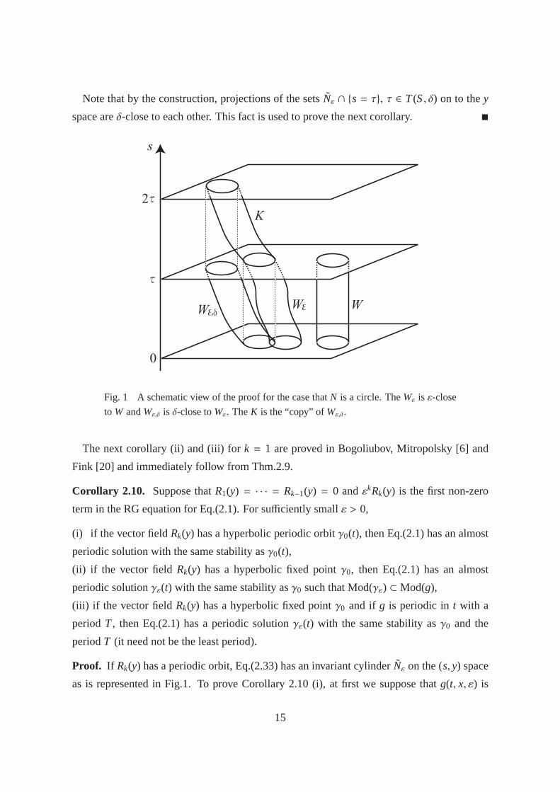
Note that by the construction, projections of the sets Nε ∩ {s = τ}, τ ∈ T (S , δ) on to the y

space are δ-close to each other. This fact is used to prove the next corollary. �

s

0

2

WW

K

W

Fig. 1 A schematic view of the proof for the case that N is a circle. The Wε is ε-close

to W and Wε,δ is δ-close to Wε. The K is the “copy” of Wε,δ.

The next corollary (ii) and (iii) for k = 1 are proved in Bogoliubov, Mitropolsky [6] and

Fink [20] and immediately follow from Thm.2.9.

Corollary 2.10. Suppose that R1(y) = · · · = Rk−1(y) = 0 and εkRk(y) is the first non-zero

term in the RG equation for Eq.(2.1). For sufficiently small ε > 0,

(i) if the vector field Rk(y) has a hyperbolic periodic orbit γ0(t), then Eq.(2.1) has an almost

periodic solution with the same stability as γ0(t),

(ii) if the vector field Rk(y) has a hyperbolic fixed point γ0, then Eq.(2.1) has an almost

periodic solution γε(t) with the same stability as γ0 such that Mod(γε) ⊂ Mod(g),

(iii) if the vector field Rk(y) has a hyperbolic fixed point γ0 and if g is periodic in t with a

period T , then Eq.(2.1) has a periodic solution γε(t) with the same stability as γ0 and the

period T (it need not be the least period).

Proof. If Rk(y) has a periodic orbit, Eq.(2.33) has an invariant cylinder Nε on the (s, y) space

as is represented in Fig.1. To prove Corollary 2.10 (i), at first we suppose that g(t, x, ε) is

15

periodic with a period T . In this case, since S (t, y, ε) is a periodic function with the period

T , Nε is periodic along the s axis in the sense that the projections S 1 := Nε ∩ {s = mT }give the same circle for all integers m. Let y = γ(t), s = t be a solution of Eq.(2.33) on the

cylinder. Then γ(mT ), m = 0, 1, · · · gives a discrete dynamics on S 1. If γ(mT ) converges

to a fixed point or a periodic orbit as m → ∞, then γ(t) converges to a periodic function as

t → ∞. Otherwise, the orbit of γ(mT ) is dense on S 1 and in this case γ(t) is an almost periodic

function. A solution of Eq.(2.1) is obtained by transforming γ(t) by the almost periodic map

α(m)t . This proves (i) of Corollary 2.10 for the case that g is periodic.

If g is almost periodic, the sets Nε ∩ {s = τ} give circles for any τ ∈ T (S , δ) and they are

δ-close to each other as is mentioned in the end of the proof of Thm.2.9. In this case, there

exists a coordinate transformation Y = ϕ(y, t) such that the cylinder Nε is straightened along

the s axis. The function ϕ is almost periodic in t because ||ϕ(y, t+ τ)−ϕ(y, t)|| is of order O(δ)

for any τ ∈ T (S , δ). Now the proof is reduced to the case that g is periodic.

The proofs of (ii) and (iii) of Corollary 2.10 are done in the same way as (i), details of

which are left to the reader. �

Remark 2.11. Suppose that the first order RG equation εR1(y) � 0 does not have normally

hyperbolic invariant manifolds but the second order RG equation εR1(y)+ε2R2(y) does. Then

can we conclude that the original system (2.1) has an invariant manifold with the same sta-

bility as that of the second order RG equation? Unfortunately, it is not true in general. For

example, suppose that the RG equation for some system is a linear equation of the form

y/ε =

(0 10 0

)y − ε

(1 00 1

)y + ε2

(0 04 0

)y + · · · , y ∈ R2. (2.38)

The origin is a fixed point of this system, however, the first term has zero eigenvalues and

we can not determine the stability up to the first order RG equation. If we calculate up to the

second order, the eigenvalues of the matrix(0 10 0

)− ε

(1 00 1

)(2.39)

are −ε (double root), so that y = 0 is a stable fixed point of the second order RG equation

if ε > 0. Unlike Corollary 2.10 (ii), this does not prove that the original system has a stable

almost periodic solution. Indeed, if we calculate the third order RG equation, the eigenvalues

of the matrix in the right hand side of Eq.(2.38) are 3ε and −ε. Therefore the origin is an

unstable fixed point of the third order RG equation. This example shows that if we truncate

higher order terms of the RG equation, stability of an invariant manifold may change and

16

we can not use εR1(y) + ε2R2(y) to investigate stability of an invariant manifold as long as

R1(y) � 0. This is because Fenichel’s theorem does not hold if the vector field f in his

theorem depends on the parameter ε.

Theorems 2.7 and 2.9 mean that the RG equation is useful to understand the properties of

the flow of the system (2.1). Since the RG equation is an autonomous system while Eq.(2.1) is

not, it seems that the RG equation is easier to analyze than the original system (2.1). Actually,

we can show that the RG equation does not lose symmetries the system (2.1) has.

Recall that integral constants in Eqs.(2.12, 14) are left undetermined and they can depend

on y (see Remark 2.4). To express the integral constants Bi(y) in Eqs.(2.12, 14) explicitly, we

rewrite them as

u(1)t (y) = B1(y) +

∫ t

(G1(s, y) − R1(y)) ds,

and

u(i)t (y) = Bi(y) +

∫ t(Gi(s, y, u

(1)s (y), · · · , u(i−1)

s (y)) −i−1∑k=1

∂u(k)s

∂y(y)Ri−k(y) − Ri(y)

)ds,

for i = 2, 3, · · · , where integral constants of the indefinite integrals in the above formulas are

chosen to be zero.

Theorem 2.12 (Inheritance of symmetries). Suppose that an ε-independent Lie group H

acts on U ⊂ M. If the vector field g and integral constants Bi(y), i = 1, · · · ,m−1 in Eqs.(2.12,

14) are invariant under the action of H; that is, they satisfy

g(t, hy, ε) =∂h∂y

(y)g(t, y, ε), Bi(hy) =∂h∂y

(y)Bi(y), (2.40)

for any h ∈ H, y ∈ U, t ∈ R and ε, then the m-th order RG equation for Eq.(2.1) is also

invariant under the action of H.

Proof. Since h ∈ H is independent of ε, Eq.(2.40) implies

gi(t, hy) =∂h∂y

(y)gi(t, y), (2.41)

for i = 1, 2, · · · . We prove by induction that Ri(y) and u(i)t (y), i = 1, 2, · · · , are invariant under

the action of H. At first, R1(hy), h ∈ H is calculated as

R1(hy) = limt→∞

1t

∫ t

G1(t, hy)ds

= limt→∞

1t

∫ t ∂h∂y

(y)G1(t, y)ds =∂h∂y

(y)R1(y). (2.42)

17

Next, u(1)t is calculated in a similar way:

u(1)t (hy) = B1(hy) +

∫ t

(G1(s, hy) − R1(hy)) ds

=∂h∂y

(y)B1(y) +∂h∂y

(y)∫ t

(G1(s, y) − R1(y)) ds

=∂h∂y

(y)u(1)t (y).

Suppose that Rk and u(k)t are invariant under the action of H for k = 1, 2, · · · , i − 1. Then, it is

easy to verify that

∂u(k)t

∂y(hy) =

∂h∂y

(y)∂u(k)

t

∂y(y)

(∂h∂y

(y)

)−1

, (2.43)

Gk(hy, u(1)t (hy), · · · , u(k−1)

t (hy)) =∂h∂y

(y)Gk(y, u(1)t (y), · · · , u(k−1)

t (y)), (2.44)

for k = 1, 2, · · · , i − 1. These equalities and Eqs.(2.13), (2.14) prove Theorem 2.12 by a

similar calculation to Eq.(2.42). �

2.3 Main theorems for autonomous systems

In this subsection, we consider an autonomous system of the form

x = f (x) + εg(x, ε)

= f (x) + εg1(x) + ε2g2(x) + · · · , x ∈ U ⊂ M, (2.45)

where the flow ϕt of f is assumed to be almost periodic due to the assumption (B) so that

Eq.(2.45) is transformed into the system of the form of (2.1). For this system, we restate

definitions and theorems obtained so far in the present notation for convenience. We also

show a few additional theorems.

Definition 2.13. Let ϕt be the flow of the vector field f . For Eq.(2.45), define the C∞ maps

Ri, h(i)t : U → M to be

R1(y) = limt→∞

1t

∫ t

(Dϕs)−1y G1(s, ϕs(y))ds, (2.46)

h(1)t (y) = (Dϕt)y

∫ t((Dϕs)

−1y G1(s, ϕs(y)) − R1(y)

)ds, (2.47)

18

and

Ri(y) = limt→∞

1t

∫ t((Dϕs)

−1y Gi(s, ϕs(y), h(1)

s (y), · · · , h(i−1)s (y))

−(Dϕs)−1y

i−1∑k=1

(Dh(k)s )yRi−k(y)

)ds, (2.48)

h(i)t (y) = (Dϕt)y

∫ t((Dϕs)

−1y Gi(s, ϕs(y), h(1)

s (y), · · · , h(i−1)s (y))

−(Dϕs)−1y

i−1∑k=1

(Dh(k)s )yRi−k(y) − Ri(y)

)ds, (2.49)

for i = 2, 3, · · · , respectively, where (Dh(k)t )y is the derivative of h(k)

t (y) with respect to y,

(Dϕt)y is the derivative of ϕt(y) with respect to y, and where Gi are defined through Eq.(2.6).

With these Ri and h(i)t , define the m-th order RG equation for Eq.(2.45) to be

y = εR1(y) + ε2R2(y) + · · · + εmRm(y), (2.50)

and define the m-th order RG transformation to be

α(m)t (y) = ϕt(y) + εh(1)

t (y) + · · · + εmh(m)t (y), (2.51)

respectively.

In the present notation, Theorems 2.5 and 2.7 are true though the relation Mod(S ) ⊂Mod(g) in Thm.2.5 (ii) is replaced by Mod(S ) ⊂ Mod(ϕt). Note that even if Eq.(2.45) is

autonomous, the function S depends on t as long as the flow ϕt depends on t.

Theorem 2.9 is refined as follows:

Theorem 2.14 (Existence of invariant manifolds). Suppose that R1(y) = · · · = Rk−1(y) = 0

and εkRk(y) is the first non-zero term in the RG equation for Eq.(2.45). If the vector field Rk(y)

has a boundaryless compact normally hyperbolic invariant manifold N, then for sufficiently

small ε > 0, Eq.(2.45) has an invariant manifold Nε, which is diffeomorphic to N. In partic-

ular, the stability of Nε coincides with that of N.

Note that unlike Thm.2.9, we need not prepare the (s, x) space, and the invariant manifold

Nε lies on M not R × M. This theorem immediately follows from the proof of Thm.2.9.

Indeed, Eq.(2.33) has an invariant manifold Nε � R × N on the (s, y) space as is shown

in the proof of Thm.2.9. An invariant manifold of Eq.(2.45) on the (s, x) is obtained by

transforming Nε by the RG transformation. However, it has to be straight along the s axis

19

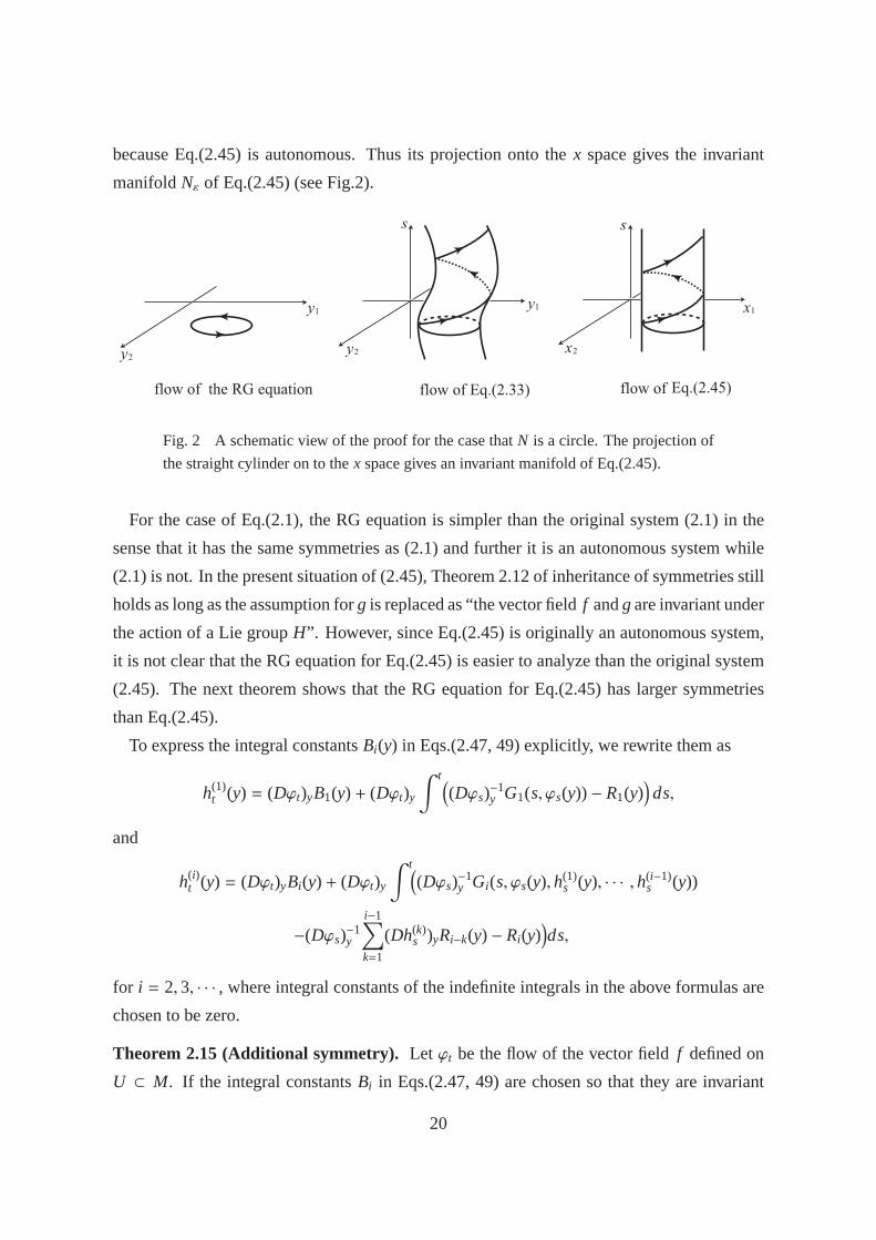
because Eq.(2.45) is autonomous. Thus its projection onto the x space gives the invariant

manifold Nε of Eq.(2.45) (see Fig.2).

y

y

s s

1y1 x1

2y2x2

Eq.(2.45)flow of the RG equation flow of Eq.(2.33) flow of

Fig. 2 A schematic view of the proof for the case that N is a circle. The projection of

the straight cylinder on to the x space gives an invariant manifold of Eq.(2.45).

For the case of Eq.(2.1), the RG equation is simpler than the original system (2.1) in the

sense that it has the same symmetries as (2.1) and further it is an autonomous system while

(2.1) is not. In the present situation of (2.45), Theorem 2.12 of inheritance of symmetries still

holds as long as the assumption for g is replaced as “the vector field f and g are invariant under

the action of a Lie group H”. However, since Eq.(2.45) is originally an autonomous system,

it is not clear that the RG equation for Eq.(2.45) is easier to analyze than the original system

(2.45). The next theorem shows that the RG equation for Eq.(2.45) has larger symmetries

than Eq.(2.45).

To express the integral constants Bi(y) in Eqs.(2.47, 49) explicitly, we rewrite them as

h(1)t (y) = (Dϕt)yB1(y) + (Dϕt)y

∫ t((Dϕs)

−1y G1(s, ϕs(y)) − R1(y)

)ds,

and

h(i)t (y) = (Dϕt)yBi(y) + (Dϕt)y

∫ t((Dϕs)

−1y Gi(s, ϕs(y), h(1)

s (y), · · · , h(i−1)s (y))

−(Dϕs)−1y

i−1∑k=1

(Dh(k)s )yRi−k(y) − Ri(y)

)ds,

for i = 2, 3, · · · , where integral constants of the indefinite integrals in the above formulas are

chosen to be zero.

Theorem 2.15 (Additional symmetry). Let ϕt be the flow of the vector field f defined on

U ⊂ M. If the integral constants Bi in Eqs.(2.47, 49) are chosen so that they are invariant

20

under the action of the one-parameter group {ϕt : U → M | t ∈ R}, then the RG equation

for Eq.(2.45) is also invariant under the action of the group. In other words, Ri satisfies the

equalityRi(ϕt(y)) = (Dϕt)yRi(y), (2.52)

for i = 1, 2, · · · .Proof. Since Eq.(2.45) is autonomous, the function Gk(t, x0, · · · , xk−1) defined through

Eq.(2.6) is independent of t and we write it as Gk(x0, · · · , xk−1). We prove by induction that

equalities Ri(ϕt(y)) = (Dϕt)yRi(y) and h(i)t (ϕt′ (y)) = h(i)

t+t′ (y) hold for i = 1, 2, · · · . For all

s′ ∈ R, R1(ϕs′ (y)) takes the form

R1(ϕs′(y)) = limt→∞

1t

∫ t

(Dϕs)−1ϕs′ (y)G1(ϕs ◦ ϕs′ (y))ds

= (Dϕs′ )y limt→∞

1t

∫ t

(Dϕs+s′)−1y G1(ϕs+s′ (y))ds.

Putting s + s′ = s′′, we verify that

R1(ϕs′(y)) = (Dϕs′ )y limt→∞

1t

∫ t+s′

(Dϕs′′ )−1y G1(ϕs′′ (y))ds′′

= (Dϕs′ )yR1(y) + (Dϕs′ )y limt→∞

1t

∫ t+s′

t(Dϕs′′ )

−1y G1(ϕs′′ (y))ds′′

= (Dϕs′ )yR1(y).

The h(1)t (ϕs′ (y)) is calculated in a similar way as

h(1)t (ϕs′ (y)) = (Dϕt)yB1(ϕs′ (y)) + (Dϕt)ϕs′ (y)

∫ t((Dϕs)

−1ϕs′ (y)G1(ϕs ◦ ϕs′(y)) − R1(ϕs′ (y))

)ds

= (Dϕt+s′ )yB1(y) + (Dϕt+s′ )y

∫ t((Dϕs+s′ )

−1y G1(ϕs+s′ (y)) − R1(y)

)ds.

Putting s + s′ = s′′ provides

h(1)t (ϕs′ (y)) = (Dϕt+s′ )yB1(y) + (Dϕt+s′ )y

∫ t+s′((Dϕs′′ )

−1y G1(ϕs′′ (y)) − R1(y)

)ds′′

= h(1)t+s′ (y). (2.53)

Suppose that Rk(ϕt(y)) = (Dϕt)yRk(y) and h(k)t (ϕt′(y)) = h(k)

t+t′ (y) hold for k = 1, 2, · · · , i − 1.

21

Then, Ri(ϕs′ (y)) is calculated as

Ri(ϕs′(y)) = limt→∞

1t

∫ t((Dϕs)

−1ϕs′ (y)Gi(ϕs ◦ ϕs′(y), h(1)

s (ϕs′(y)), · · · , h(i−1)s (ϕs′(y)))

−(Dϕs)−1ϕs′ (y)

i−1∑k=1

(Dh(k)s )ϕs′ (y)Ri−k(ϕs′(y))

)ds

= (Dϕs′ )y limt→∞

1t

∫ t((Dϕs+s′)

−1y Gi(ϕs+s′ (y), h(1)

s+s′(y), · · · , h(i−1)s+s′ (y))

−(Dϕs+s′ )−1y

i−1∑k=1

(Dh(k)s+s′ )yRi−k(y)

)ds.

Putting s + s′ = s′′ provides

Ri(ϕs′ (y)) = (Dϕs′ )y limt→∞

1t

∫ t+s′((Dϕs′′ )

−1y Gi(ϕs′′ (y), h(1)

s′′ (y), · · · , h(i−1)s′′ (y))

−(Dϕs′′ )−1y

i−1∑k=1

(Dh(k)s′′ )yRi−k(y)

)ds′′

= (Dϕs′ )yRi(y) + (Dϕs′ )y limt→∞

1t

∫ t+s′

t

((Dϕs′′ )

−1y Gi(ϕs′′ (y), h(1)

s′′ (y), · · · , h(i−1)s′′ (y))

−(Dϕs′′ )−1y

i−1∑k=1

(Dh(k)s′′ )yRi−k(y)

)ds′′

= (Dϕs′ )yRi(y).

We can show the equality h(i)t (ϕt′(y)) = h(i)

t+t′ (y) in a similar way. �

2.4 Simplified RG equation

Recall that the definitions of Ri and u(i)t given in Eqs.(2.11) to (2.14) include the indefinite

integrals and we have left the integral constants undetermined (see Rem.2.4). In this subsec-

tion, we investigate how different choices of the integral constants change the forms of RG

equations and RG transformations.

Let us fix definitions of Ri and u(i)t , i = 1, 2, · · · by fixing integral constants in Eqs.(2.12,

14) arbitrarily (note that Ri and u(i)t are independent of the integral constants in Eqs.(2.11,

13)). For these Ri and u(i)t , we define Ri and u(i)

t to be

R1(y) = limt→∞

1t

∫ t

G1(s, y)ds, (2.54)

u(1)t (y) = B1(y) +

∫ t(G1(s, y) − R1(y)

)ds, (2.55)

22

and

Ri(y) = limt→∞

1t

∫ t(Gi(s, y, u

(1)s (y), · · · , u(i−1)

s (y)) −i−1∑k=1

∂u(k)s

∂y(y)Ri−k(y)

)ds, (2.56)

u(i)t (y) = Bi(y) +

∫ t(Gi(s, y, u

(1)s (y), · · · , u(i−1)

s (y)) −i−1∑k=1

∂u(k)s

∂y(y)Ri−k(y) − Ri(y)

)ds,(2.57)

for i = 2, 3, · · · , respectively, where integral constants in the definitions of u(i)t are the same

as those of u(i)t and where Bi, i = 1, 2, · · · are arbitrary vector fields which imply other choice

of integral constants. Along with these functions, We define the m-th order RG equation and

the m-th order RG transformation to be

y = εR1(y) + · · · + εmRm(y), (2.58)

andα(m)

t (y) = y + εu(1)t (y) + · · · + εmu(m)

t (y), (2.59)

respectively. Now we have two pairs of RG equations-transformations, Eqs.(2.18),(2.19) and

Eqs.(2.58),(2.59). Main theorems described so far hold for both of them for any choices of

Bi(y)’s except to Thms. 2.11 and 2.15, in which we need additional assumptions for Bi(y)’s

as was stated.

Let us examine relations between Ri, u(i)t and Ri, u(i)

t . Clearly R1 coincides with R1. Thus

u(1)t is given as u(1)

t (y) = u(1)t (y) + B1(y). According to the definition of G2 (Eq.(2.8)), R2 is

calculated as

R2(y) = limt→∞

1t

∫ t∂g1

∂y(s, y)u(1)

s (y) + g2(s, y) − ∂u(1)s

∂yR1(y)

ds

= limt→∞

1t

∫ t∂g1

∂y(s, y)u(1)

s (y) + g2(s, y) − ∂u(1)s

∂yR1(y)

ds

+ limt→∞

1t

∫ t(∂g1

∂y(s, y)B1(y) − ∂B1

∂y(y)R1(y)

)ds

= R2(y) +∂R1

∂y(y)B1(y) − ∂B1

∂y(y)R1(y). (2.60)

If we define the commutator [ · , · ] of vector fields to be

[B1,R1](y) =∂B1

∂y(y)R1(y) − ∂R1

∂y(y)B1(y), (2.61)

Eq.(2.60) is rewritten asR2(y) = R2(y) − [B1,R1](y). (2.62)

23

Similar calculation proves that Ri, i = 2, 3, · · · are expressed as

Ri(y) = Ri(y) + Pi(R1, · · · ,Ri−1, B1, · · · , Bi−2)(y) − [Bi−1,R1](y), (2.63)

where Pi is a function of R1, · · · ,Ri−1 and B1, · · · , Bi−2. See Chiba[11] for the proof. Thus

appropriate choices of vector fields Bi(y), i = 1, 2, · · · may simplify Ri, i = 2, 3, · · · through

Eq.(2.63).

Suppose that Ri, i = 1, 2, · · · are elements of some finite dimensional vector space V and

the commutator [ · ,R1] defines the linear map on V . For example if the function g(t, x, ε)

in Eq.(2.1) is polynomial in x, V is the space of polynomial vector fields. If Eq.(2.1) is an

n-dimensional linear equation, then V is the space of all n×n constant matrices. Let us take a

complementary subspace C to Im [ · ,R1] into V arbitrarily: V = Im [ · ,R1]⊕C. Then, there

exist Bi ∈ V, i = 1, 2, · · · ,m − 1 such that Ri ∈ C for i = 2, 3, · · · ,m because of Eq.(2.63).

If Ri ∈ C for i = 2, 3, · · · ,m, we call Eq.(2.58) the m-th order simplified RG equation.

See Chiba[11] for explicit forms of the simplified RG equation for the cases that Eq.(2.1)

is polynomial in x or a linear system. In particular, they are quite related to the simplified

normal forms theory (hyper-normal forms theory) [2,39,40]. See also Section 4.3.

Since integral constants Bi’s in Eqs.(2.55) and (2.57) are independent of t, we can show the

next claim, which will be used to prove Thm.5.1.

Claim 2.16. RG equations and RG transformations are not unique in general because of

undetermined integral constants in Eqs.(2.12) and (2.14). Let α(m)t and α(m)

t be two different

RG transformations for a given system (2.1). Then, there exists a time-independent trans-

formation φ(y, ε), which is C∞ with respect to y and ε, such that α(m)t (y) = α(m)

t ◦ φ(y, ε).

Conversely, α(m)t ◦ φ(y, ε) gives one of the RG transformations for any C∞ maps φ(y, ε).

Note that the map φ(y, ε) is independent of t because it brings one of the RG equations into

the other RG equation, both of which are autonomous systems. According to Claim 2.16, one

of the simplest way to achieve simplified RG equations is as follows: At first, we calculate

Ri and u(i)t by fixing integral constants arbitrarily and obtain the RG equation. It may be

convenient in practice to choose zeros as integral constants (see Prop.2.18 below). Then, any

other RG equations are given by transforming the present RG equation by time-independent

C∞ maps.

24

2.5 An example

In this subsection, we give an example to verify the main theorems. See Chiba[10,11] for

more examples. Consider the system on R2

{X1 = X2 + X2

2 + ε2k sin(ωt),

X2 = −X1 + ε2X2 − X1X2 + X2

2 ,(2.64)

where ε > 0, k ≥ 0 and ω > 0 are parameters. Changing the coordinates by (X1, X2) =

(εx1, εx2) yields {x1 = x2 + εx2

2 + εk sin(ωt),x2 = −x1 + ε(x2

2 − x1x2) + ε2x2.(2.65)

Diagonalizing the unperturbed term by introducing the complex variable z as x1 = z+ z, x2 =

i(z − z) may simplify our calculation :z = iz +

ε

2

(i(z − z)2 − 2z2 + 2zz + k sin(ωt)

)+ε2

2(z − z),

z = −iz +ε

2

(−i(z − z)2 − 2z2

+ 2zz + k sin(ωt))− ε

2

2(z − z),

(2.66)

where i =√−1. Let us calculate the RG equation for the system (2.65) or (2.66). In this

example, all integral constants in Eqs.(2.47, 49) are chosen to be zero.

(i) When ω � 1, 2, the second order RG equation for Eq.(2.66) is given asy1 =

12ε2(y1 − 3y2

1y2 − 16i3

y21y2),

y2 =12ε2(y2 − 3y1y2

2 +16i3

y1y22),

(2.67)

where the first order RG equation R1 vanishes. Note that it is independent of the time periodic

external force k sin(ωt). Thus this RG equation coincides with that of the autonomous system

obtained by putting k = 0 in Eq.(2.66) and Theorem 2.15 is applicable to Eq.(2.67). Indeed,

since the above RG equation is invariant under the rotation group (y1, y2) → (eiτy1, e−iτy2),

putting y1 = reiθ, y2 = re−iθ results inr =

12ε2r(1 − 3r2),

θ = −83ε2r2,

(2.68)

and it is easily solved. We can verify that this RG equation has a stable periodic orbit r =√1/3 if ε > 0. Now Corollary 2.10 (i) proves that the original system (2.65) has a stable

25

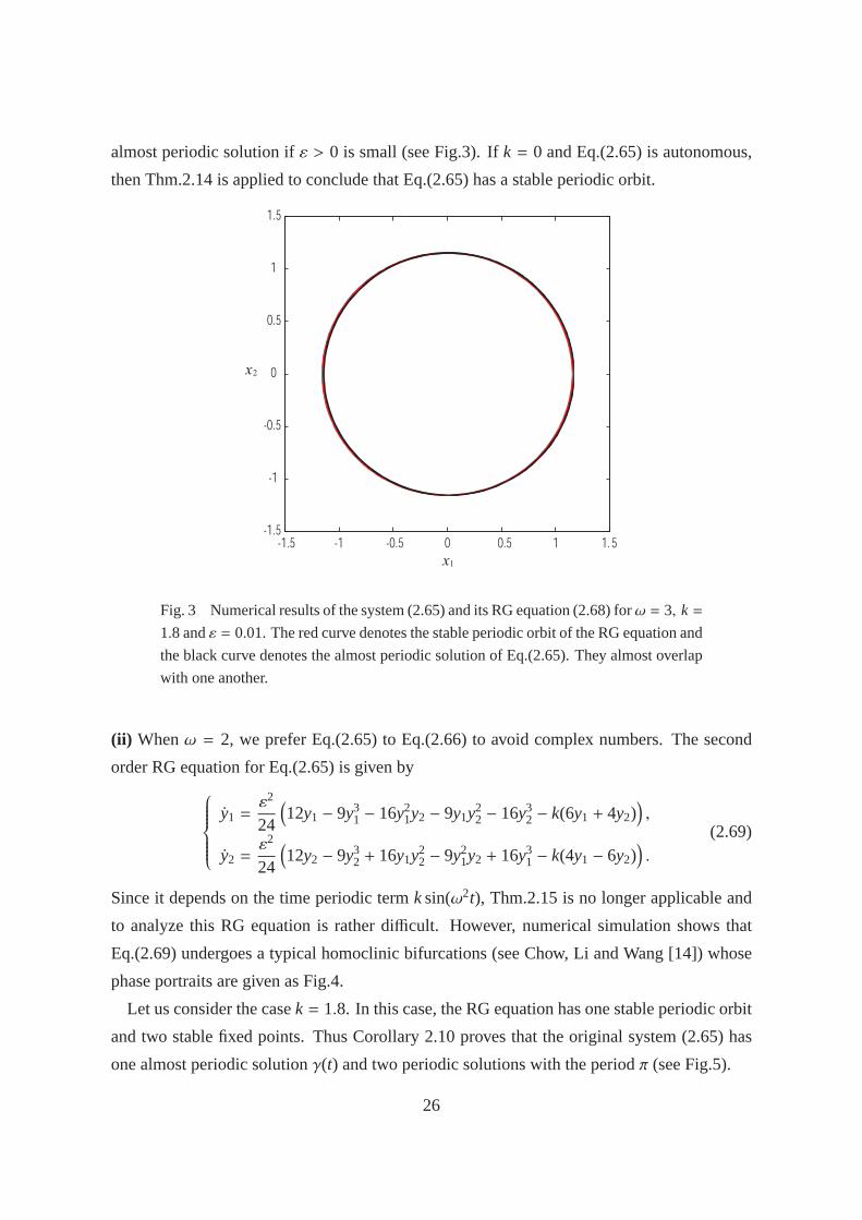
almost periodic solution if ε > 0 is small (see Fig.3). If k = 0 and Eq.(2.65) is autonomous,

then Thm.2.14 is applied to conclude that Eq.(2.65) has a stable periodic orbit.

-1.5

-1

-0.5

0

0.5

1

1.5

-1.5 -1 -0.5 0 0.5 1 1.5x1

x2

Fig. 3 Numerical results of the system (2.65) and its RG equation (2.68) forω = 3, k =

1.8 and ε = 0.01. The red curve denotes the stable periodic orbit of the RG equation and

the black curve denotes the almost periodic solution of Eq.(2.65). They almost overlap

with one another.

(ii) When ω = 2, we prefer Eq.(2.65) to Eq.(2.66) to avoid complex numbers. The second

order RG equation for Eq.(2.65) is given byy1 =

ε2

24

(12y1 − 9y3

1 − 16y21y2 − 9y1y2

2 − 16y32 − k(6y1 + 4y2)

),

y2 =ε2

24

(12y2 − 9y3

2 + 16y1y22 − 9y2

1y2 + 16y31 − k(4y1 − 6y2)

).

(2.69)

Since it depends on the time periodic term k sin(ω2t), Thm.2.15 is no longer applicable and

to analyze this RG equation is rather difficult. However, numerical simulation shows that

Eq.(2.69) undergoes a typical homoclinic bifurcations (see Chow, Li and Wang [14]) whose

phase portraits are given as Fig.4.

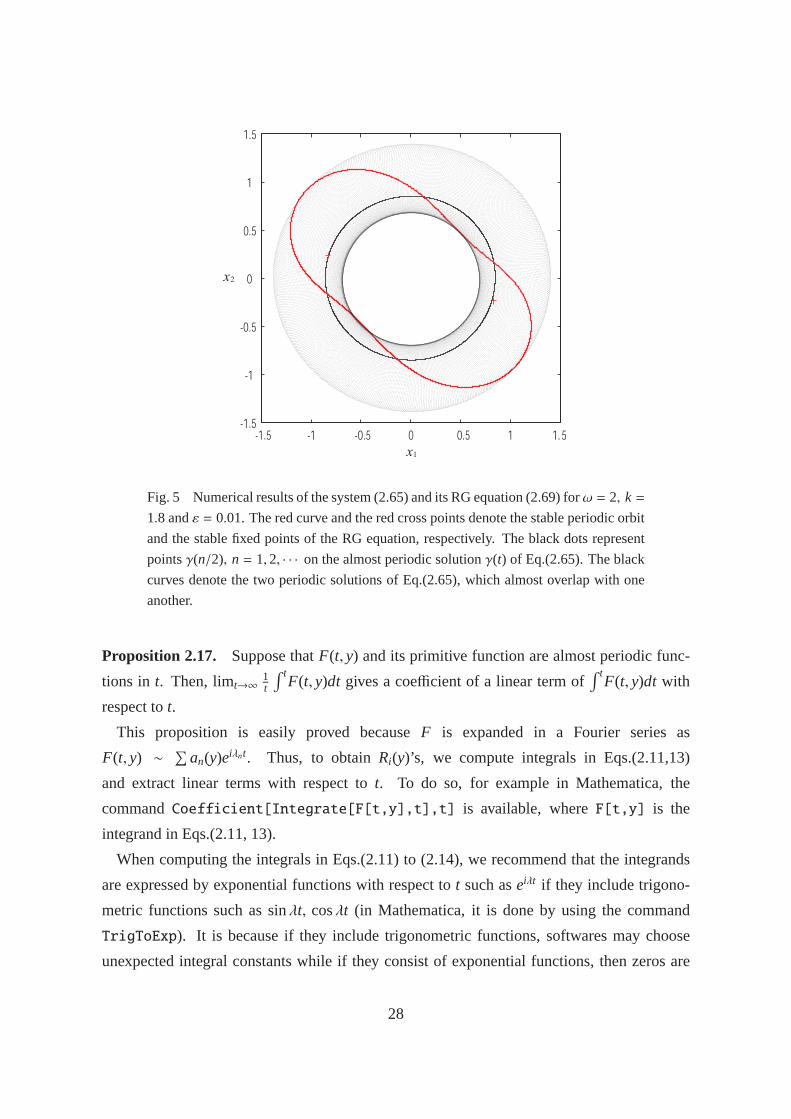
Let us consider the case k = 1.8. In this case, the RG equation has one stable periodic orbit

and two stable fixed points. Thus Corollary 2.10 proves that the original system (2.65) has

one almost periodic solution γ(t) and two periodic solutions with the period π (see Fig.5).

26

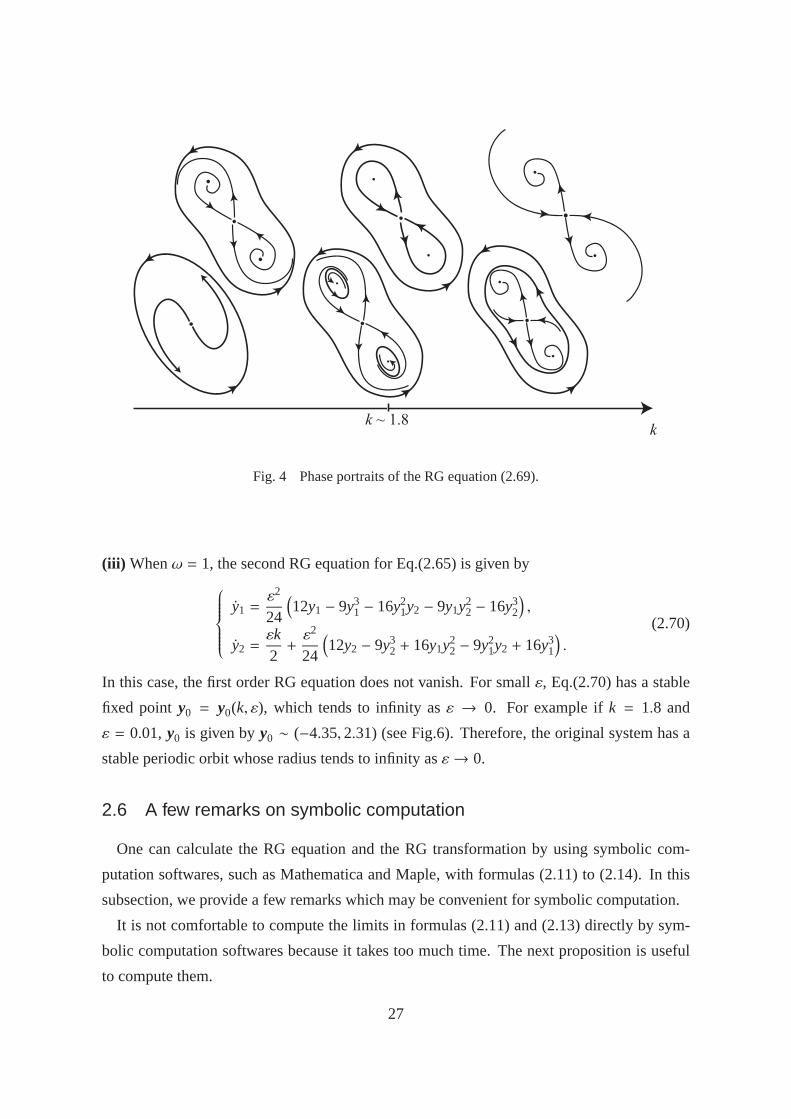
kk ~ 1.8

Fig. 4 Phase portraits of the RG equation (2.69).

(iii) When ω = 1, the second RG equation for Eq.(2.65) is given byy1 =

ε2

24

(12y1 − 9y3

1 − 16y21y2 − 9y1y2

2 − 16y32

),

y2 =εk2+ε2

24

(12y2 − 9y3

2 + 16y1y22 − 9y2

1y2 + 16y31

).

(2.70)

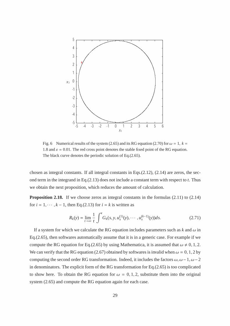
In this case, the first order RG equation does not vanish. For small ε, Eq.(2.70) has a stable

fixed point y0 = y0(k, ε), which tends to infinity as ε → 0. For example if k = 1.8 and

ε = 0.01, y0 is given by y0 ∼ (−4.35, 2.31) (see Fig.6). Therefore, the original system has a

stable periodic orbit whose radius tends to infinity as ε→ 0.

2.6 A few remarks on symbolic computation

One can calculate the RG equation and the RG transformation by using symbolic com-

putation softwares, such as Mathematica and Maple, with formulas (2.11) to (2.14). In this

subsection, we provide a few remarks which may be convenient for symbolic computation.

It is not comfortable to compute the limits in formulas (2.11) and (2.13) directly by sym-

bolic computation softwares because it takes too much time. The next proposition is useful

to compute them.

27

-1.5

-1

-0.5

0

0.5

1

1.5

-1.5 -1 -0.5 0 0.5 1 1.5x1

x2

Fig. 5 Numerical results of the system (2.65) and its RG equation (2.69) forω = 2, k =

1.8 and ε = 0.01. The red curve and the red cross points denote the stable periodic orbit

and the stable fixed points of the RG equation, respectively. The black dots represent

points γ(n/2), n = 1, 2, · · · on the almost periodic solution γ(t) of Eq.(2.65). The black

curves denote the two periodic solutions of Eq.(2.65), which almost overlap with one

another.

Proposition 2.17. Suppose that F(t, y) and its primitive function are almost periodic func-

tions in t. Then, limt→∞ 1t

∫ tF(t, y)dt gives a coefficient of a linear term of

∫ tF(t, y)dt with

respect to t.

This proposition is easily proved because F is expanded in a Fourier series as

F(t, y) ∼ ∑an(y)eiλnt. Thus, to obtain Ri(y)’s, we compute integrals in Eqs.(2.11,13)

and extract linear terms with respect to t. To do so, for example in Mathematica, the

command Coefficient[Integrate[F[t,y],t],t] is available, where F[t,y] is the

integrand in Eqs.(2.11, 13).

When computing the integrals in Eqs.(2.11) to (2.14), we recommend that the integrands

are expressed by exponential functions with respect to t such as eiλt if they include trigono-

metric functions such as sin λt, cos λt (in Mathematica, it is done by using the command

TrigToExp). It is because if they include trigonometric functions, softwares may choose

unexpected integral constants while if they consist of exponential functions, then zeros are

28

-5

-4

-3

-2

-1

0

1

2

3

4

5

-5 -4 -3 -2 -1 0 1 2 3 4 5 6x1

x2

Fig. 6 Numerical results of the system (2.65) and its RG equation (2.70) forω = 1, k =

1.8 and ε = 0.01. The red cross point denotes the stable fixed point of the RG equation.

The black curve denotes the periodic solution of Eq.(2.65).

chosen as integral constants. If all integral constants in Eqs.(2.12), (2.14) are zeros, the sec-

ond term in the integrand in Eq.(2.13) does not include a constant term with respect to t. Thus

we obtain the next proposition, which reduces the amount of calculation.

Proposition 2.18. If we choose zeros as integral constants in the formulas (2.11) to (2.14)

for i = 1, · · · , k − 1, then Eq.(2.13) for i = k is written as

Rk(y) = limt→∞

1t

∫ t

Gk(s, y, u(1)s (y), · · · , u(k−1)

s (y))ds. (2.71)

If a system for which we calculate the RG equation includes parameters such as k and ω in

Eq.(2.65), then softwares automatically assume that it is in a generic case. For example if we

compute the RG equation for Eq.(2.65) by using Mathematica, it is assumed that ω � 0, 1, 2.

We can verify that the RG equation (2.67) obtained by softwares is invalid whenω = 0, 1, 2 by

computing the second order RG transformation. Indeed, it includes the factors ω,ω−1, ω−2

in denominators. The explicit form of the RG transformation for Eq.(2.65) is too complicated

to show here. To obtain the RG equation for ω = 0, 1, 2, substitute them into the original

system (2.65) and compute the RG equation again for each case.

29

3 Restricted RG method

Suppose that Eq.(2.3) defined on U ⊂ M does not satisfy the assumption (B) on U but

satisfies it on a submanifold N0 ⊂ U. Then, the RG method discussed in the previous sec-

tion is still valid if domains of the RG equation and the RG transformation are restricted to

N0. This method to construct an approximate flow on some restricted region is called the

restricted RG method and it gives extension of the center manifold theory, the geometric

singular perturbation method and the phase reduction.

3.1 Main results of the restricted RG method

Consider the system of the form

x = f (x) + εg(t, x, ε), (3.1)

defined on U ⊂ M. For this system, we suppose that

(D1) the vector field f is C∞ and it has a compact attracting normally hyperbolic invariant

manifold N0 ⊂ U. The flow ϕt(x) of f on N0 is an almost periodic function with respect to

t ∈ R uniformly in x ∈ N0, the set of whose Fourier exponents has no accumulation points.

(D2) there exists an open set V ⊃ N0 in U such that the vector field g is C1 in t ∈ R, C∞ in

x ∈ V and small ε, and that g is an almost periodic function with respect to t ∈ R uniformly

in x ∈ V and small ε, the set of whose Fourier exponents has no accumulation points (i.e. the

assumption (A) is satisfied on V).

If g is independent of t and Eq.(3.1) is autonomous, Fenichel’s theorem proves that Eq.(3.1)

has an attracting invariant manifold Nε near N0. If g depends on t, we rewrite Eq.(3.1) as{x = f (x) + εg(s, x, ε),s = 1,

(3.2)

so that the unperturbed term ( f (x), 1) has an attracting normally hyperbolic invariant manifold

R × N0 on the (s, x) space. Then, a similar argument to the proof of Thm.2.9 proves that

Eq.(3.2) has an attracting invariant manifold Nε on the (s, x) space, which is diffeomorphic to

R × N0.

In both cases, since Nε is attracting, long time behavior of the flow of Eq.(3.1) is well

described by the flow on Nε. Thus a central issue is to construct Nε and the flow on it

30

approximately. To do so, we establish the restricted RG method on N0.

Definition 3.1. For Eq.(3.1), we define C∞ maps Ri, h(i)t : N0 → M to be

R1(y) = limt→−∞

1t

∫ t

(Dϕs)−1y G1(s, ϕs(y))ds, (3.3)

h(1)t (y) = (Dϕt)y

∫ t

−∞

((Dϕs)

−1y G1(s, ϕs(y)) − R1(y)

)ds, (3.4)

and

Ri(y) = limt→−∞

1t

∫ t((Dϕs)

−1y Gi(s, ϕs(y), h(1)

s (y), · · · , h(i−1)s (y))

−(Dϕs)−1y

i−1∑k=1

(Dh(k)s )yRi−k(y)

)ds, (3.5)

h(i)t (y) = (Dϕt)y

∫ t

−∞

((Dϕs)

−1y Gi(s, ϕs(y), h(1)

s (y), · · · , h(i−1)s (y))

−(Dϕs)−1y

i−1∑k=1

(Dh(k)s )yRi−k(y) − Ri(y)

)ds, (3.6)

for i = 2, 3, · · · , respectively. Note that limt→∞ in Eqs.(2.46, 48) are replaced by limt→−∞ and

the indefinite integrals in Eqs.(2.47, 49) are replaced by the definite integrals. With these Ri

and h(i)t , define the restricted m-th order RG equation for Eq.(3.1) to be

y = εR1(y) + ε2R2(y) + · · · + εmRm(y), y ∈ N0, (3.7)

and define the restricted m-th order RG transformation to be

αt(y) = ϕt(y) + εh(1)t (y) + · · · + εmh(m)

t (y), y ∈ N0, (3.8)

respectively.

Note that the domains of them are restricted to N0. To see that they make sense, we prove

the next lemma, which corresponds to Lemma 2.1.

Lemma 3.2. (i) The maps Ri (i = 1, 2, · · · ) are well-defined and Ri(y) ∈ TyN0 for any y ∈ N0.

(ii) The maps h(i)t (i = 1, 2, · · · ) are almost periodic functions with respect to t uniformly in

y ∈ N0. In particular, h(i)t are bounded in t ∈ R if y ∈ N0.

Proof. Let πs be the projection from TyM to the stable subspace Es of N0 and πN0 the

projection from TyM to the tangent space TyN0. Note that πs + πN0 = id. By the definition of

an attracting hyperbolic invariant manifold, there exist positive constants C1 and α such that

||πs(Dϕt)−1y v|| < C1eαt ||v||, (3.9)

31

for any t < 0, y ∈ N0 and v ∈ TyM. Since ϕt(y) ∈ N0 for all t ∈ R and since G1 is almost

periodic in t, there exists a positive constant C2 such that ||G1(t, ϕt(y))|| < C2. Then, πsR1(y)

proves to satisfy

||πsR1(y)|| ≤ limt→−∞

1t

∫ t

||πs(Dϕs)−1y G1(s, ϕs(y))||ds

< limt→−∞

1t

∫ t

C1C2eαsds = 0. (3.10)

This means that R1(y) ∈ TyN0.

To prove (ii) of Lemma 3.2, note that the set

T (δ) = {τ | ||G1(s + τ, y) −G1(s, y)|| < δ, ||ϕs+τ(y) − ϕs(y)|| < δ, ∀s ∈ R, ∀y ∈ N0} (3.11)

is relatively dense. For τ ∈ T (δ), h(1)t (ϕτ(y)) is calculated as

h(1)t (ϕτ(y)) = (Dϕt)ϕτ(y)

∫ t

−∞

((Dϕs)

−1ϕτ(y)G1(s, ϕs ◦ ϕτ(y)) − R1(ϕτ(y))

)ds

=

∫ t

−∞

((Dϕs−t)

−1y G1(s, ϕs+τ(y)) − (Dϕt)ϕτ(y)R1(ϕτ(y))

)ds. (3.12)

Putting s′ = s + τ yields

h(1)t (ϕτ(y)) =

∫ t+τ

−∞

((Dϕs′−(t+τ))

−1y G1(s′ − τ, ϕs′(y)) − (Dϕt)ϕτ(y)R1(ϕτ(y))

)ds′. (3.13)

Since the space TyN0 is (Dϕt)y-invariant, πs(Dϕt)yR1(y) = 0. This and Eq.(3.13) provide that

||πsh(1)t+τ(y) − πsh

(1)t (ϕτ(y))|| ≤

∫ t+τ

−∞||πs(Dϕs−(t+τ))

−1y || · ||G1(s, ϕs(y)) −G1(s − τ, ϕs(y))||ds

≤∫ t+τ

−∞δC1eα(s−(t+τ))ds = δC1/α. (3.14)

Thus we obtain

||πsh(1)t+τ(y) − πsh

(1)t (y)|| ≤ ||πsh

(1)t+τ(y) − πsh

(1)t (ϕτ(y))|| + ||πsh

(1)t (ϕτ(y)) − πsh

(1)t (y)||

≤ (C1/α + Lt)δ,

where Lt, which is bounded in t, is the Lipschitz constant of πsh(1)t |N0 . This proves that πsh

(1)t

is an almost periodic function with respect to t. On the other hand, πN0h(1)t is written as

πN0h(1)t (y) = πN0 (Dϕt)y

∫ t

−∞

(πN0 (Dϕs)

−1y G1(s, ϕs(y)) − R1(y)

)ds. (3.15)

Since πN0 (Dϕt)y is almost periodic, we can show that πN0h(1)t (y) is almost periodic in t in the

same way as the proof of Lemma 2.1 (ii). This proves that h(1)t = πsh

(1)t + πN0h

(1)t is an almost

32

periodic function in t. The proof of Lemma 3.2 for i = 2, 3, · · · is done in a similar way by

induction and we omit it here. �

Since Ri(y) ∈ TyN0, Eq.(3.7) defines a dimN0-dimensional differential equation on N0.

Remark 3.3. Even if h(i)t are defined by using indefinite integrals as Eqs.(2.47, 49), we can

show that h(i)t is bounded as t → ∞, though it is not bounded as t → −∞. In this case, the

theorems listed below are true for large t.

Now we are in a position to state main theorems of the restricted RG method, all proofs of

which are the same as before and omitted.

Theorem 3.4. Let α(m)t be the restricted m-th order RG transformation for Eq.(3.1). If |ε| is

sufficiently small, there exists a function S (t, y, ε), y ∈ N0 such that

(i) by changing the coordinates as x = α(m)t (y), Eq.(3.1) is transformed into the system

y = εR1(y) + ε2R2(y) + · · · + εmRm(y) + εm+1S (t, y, ε), (3.16)

(ii) S is an almost periodic function with respect to t uniformly in y ∈ N0,

(iii) S (t, y, ε) is C1 with respect to t and C∞ with respect to y ∈ N0 and ε.

Theorem 3.5 (Error estimate). Let y(t) be a solution of the restricted m-th order RG

equation and α(m)t the restricted m-th order RG transformation. There exist positive constants

ε0,C and T such that a solution x(t) of Eq.(3.1) with x(0) = α(m)0 (y(0)) ∈ α(m)

0 (N0) satisfies the

inequality||x(t) − α(m)

t (y(t))|| < C|ε|m, (3.17)

for |ε| < ε0 and 0 ≤ t ≤ T/|ε|.Theorem 3.6 (Existence of invariant manifolds). Suppose that R1(y) = · · · = Rk−1(y) = 0

and εkRk(y) is the first non-zero term in the restricted RG equation for Eq.(3.1). If the vector

field Rk(y) has a boundaryless compact normally hyperbolic invariant manifold L ⊂ N0, then

for sufficiently small ε > 0, the system (3.2) has an invariant manifold Lε on the (s, x) space

which is diffeomorphic to R × L. In particular, the stability of Lε coincides with that of L.

Theorem 3.7 (Inheritance of symmetries). Suppose that an ε-independent Lie group H

acts on N0. If the vector field f and g are invariant under the action of H, then the restricted

m-th order RG equation for Eq.(3.1) is also invariant under the action of H.

Recall that our purpose is to construct the invariant manifold Nε of Eq.(3.1) and the flow

on Nε approximately. The flow on Nε is well understood by Theorems 3.4 to 3.6, and Nε is

33

given by the next theorem.

Theorem 3.8. Let α(m)t be the restricted m-th order RG transformation for Eq.(3.1). Then,

the set {(t, x) | x ∈ α(m)t (N0)} lies within an O(εm+1) neighborhood of the attracting invariant

manifold Nε of Eq.(3.2).

Proof. Though the maps Ri(y) and α(m)t are defined on N0, we can extend them to the maps

defined on V ⊃ N0 so that Eq.(3.7) is C1 close to Eq.(3.16) on V and that N0 is an attracting

normally hyperbolic invariant manifold of Eq.(3.7). Then the same argument as the proof of

Thm.2.9 proves Theorem 3.8. �

If the vector field g is independent of t and Eq.(3.1) is autonomous, we can prove the next

theorems.

Theorem 3.9 (Existence of invariant manifolds). Suppose that R1(y) = · · · = Rk−1(y) =

0 and εkRk(y) is the first non-zero term in the restricted RG equation for Eq.(3.1) with t-

independent g. If the vector field Rk(y) has a boundaryless compact normally hyperbolic

invariant manifold L, then for sufficiently small ε > 0, Eq.(3.1) has an invariant manifold Lε,

which is diffeomorphic to L. In particular, the stability of Lε coincides with that of L.

Theorem 3.10 (Additional symmetry). The restricted RG equation for Eq.(3.1) with t-

independent g is invariant under the action of the one-parameter group {ϕt : N0 → N0 | t ∈ R}.In other words, Ri satisfies the equality

Ri(ϕt(y)) = (Dϕt)yRi(y), y ∈ N0, (3.18)

for i = 1, 2, · · · .

For autonomous systems, Thm.3.8 is restated as follows: Recall that if the function g

depends on t, the attracting invariant manifold Nε of Eq.(3.1) and the approximate invariant

manifold described in Thm.3.8 depend on t in the sense that they lie on the (s, x) space. If

Eq.(3.1) is autonomous, its attracting invariant manifold Nε lies on M and is independent

of t. Thus we want to construct an approximate invariant manifold of Nε so that it is also

independent of t.

Theorem 3.11. Let α(m)t be the restricted m-th order RG transformation for Eq.(3.1). If g is

independent of t, the set α(m)t (N0) = {α(m)

t (y) | y ∈ N0} is independent of t and lies within an

O(εm+1) neighborhood of the attracting invariant manifold Nε of Eq.(3.1).

34

Proof. We have to show that the set α(m)t (N0) is independent of t. Indeed, we know the

equality h(i)t (ϕt′ (y)) = h(i)

t+t′(y) as is shown in the proof of the Thm.2.15. This proves that

α(m)t+t′ (N0) = α(m)

t (ϕt′ (N0)) = α(m)t (N0). (3.19)

The rest of the proof is the same as the proofs of Thm.2.14 and Thm.3.8. �

3.2 Center manifold reduction

The restricted RG method recovers the approximation theory of center manifolds (Carr

[7]). Consider a system of the form

x = Fx + εg(x, ε)

= Fx + εg1(x) + ε2g2(x) + · · · , x ∈ Rn, (3.20)

where unperturbed term Fx is linear. For this system, we suppose that

(E1) all eigenvalues of the n × n constant matrix F are on the imaginary axis or the left half

plane. The Jordan block corresponding to eigenvalues on the imaginary axis is diagonaliz-

able.

(E2) g is C∞ with respect to x and ε such that g(0, ε) = 0.

If all eigenvalues of F are on the left half plane, the origin is a stable fixed point and the flow

near the origin is trivial. In what follows, we suppose that at least one eigenvalue is on the

imaginary axis. In this case, Eq.(3.20) has a center manifold which is tangent to the center

subspace N0 at the origin. The center subspace N0, which is spanned by eigenvectors asso-

ciated with eigenvalues on the imaginary axis, is an attracting normally hyperbolic invariant

manifold of the unperturbed term Fx, and the flow of Fx on N0 is almost periodic. However,

since N0 is not compact, we take an n-dimensional closed ball K including the origin and

consider N0 ∩ K. Then, we obtain the next theorem as a corollary of Thm.3.9 and Thm.3.11.

Theorem 3.12 (Approximation of Center Manifolds, [12]). Let α(m)t be the restricted m-th

order RG transformation for Eq.(3.20) and K a small compact neighborhood of the origin.

Then, the set α(m)t (K ∩ N0) lies within an O(εm+1) neighborhood of the center manifold of

Eq.(3.20). The flow of Eq.(3.20) on the center manifold is well approximated by those of the

restricted RG equation. In particular, suppose that R1(y) = · · · = Rk−1(y) = 0 and εkRk(y) is

the first non-zero term in the restricted RG equation. If the vector field Rk(y) has a bound-

aryless compact normally hyperbolic invariant manifold L, then for sufficiently small ε > 0,

35

Eq.(3.20) has an invariant manifold Lε on the center manifold, which is diffeomorphic to L.

The stability of Lε coincides with that of L.

See Chiba [12] for the detail of the proof and examples.

3.3 Geometric singular perturbation method

The restricted RG method can also recover the geometric singular perturbation method

proposed by Fenichel [19].

Consider the autonomous system

x = f (x) + εg(x, ε), x ∈ Rn (3.21)

on Rn with the assumption that

(F) suppose that f and g are C∞ with respect to x and ε, and that f has an m-dimensional

attracting normally hyperbolic invariant manifold N0 which consists of fixed points of f ,

where m < n.

Note that this system satisfies the assumptions (D1) and (D2), so that Thm.3.9 to Thm.3.11

hold. The invariant manifold N0 consisting of fixed points of the unperturbed system is called

the critical manifold (see [1]). For this system, Fenichel[19] proved that there exist local

coordinates (u, v) such that the system (3.21) is expressed as{u = εg1(u, v, ε), u ∈ Rm,

v = f (u, v) + εg2(u, v, ε), v ∈ Rn−m,(3.22)

where f (u, 0) = 0 for any u ∈ Rm. In this coordinate, the critical manifold N0 is locally given

as the u-plane. Further he proved the next theorem.

Theorem 3.13 (Fenichel [19]). Suppose that the system u = εg1(u, 0, 0) has a compact

normally hyperbolic invariant manifold L. If ε > 0 is sufficiently small, the system (3.22) has

an invariant manifold Lε which is diffeomorphic to L.

This method to obtain an invariant manifold of (3.22) is called the geometric singular

perturbation method. By using the fact that ϕt(u) = u for u ∈ N0, it is easy to verify that

the system u = εg1(u, 0, 0) described above is just the restricted first order RG equation for

Eq.(3.22). Thus Thm.3.13 immediately follows from Thm.3.9. Note that in our method, we

36

need not change the coordinates so that Eq.(3.21) is transformed into the form of Eq.(3.22).

Example 3.14.　 Consider the system on R2

{x1 = −x1 + (x1 + c)x2,εx2 = x1 − (x1 + 1)x2,

(3.23)

where 0 < c < 1 is a constant. This system arises from a model of the kinetics of enzyme

reactions (see Carr [7]). Set t = εs and denote differentiation with respect to s by ′ . Then,

the above system is rewritten as{x′1 = ε(−x1 + cx2 + x1x2),x′2 = x1 − x2 − x1x2.

(3.24)

The attracting critical manifold N0 of this system is expressed as the graph of the function

x2 = h(x1) :=x1

1 + x1. (3.25)

Since the restricted first order RG transformation for Eq.(3.24) is given by

α(1)t (y1) =

(y1

y1/(1 + y1)

)+ ε

(0

−(c − 1)y1/(1 + y1)4

), (3.26)

Theorem 3.11 proves that the attracting invariant manifold of Eq.(3.24) is given as the graph

of

x2 =x1

1 + x1− ε (c − 1)x1

(1 + x1)4+ O(ε2). (3.27)

If |x1| is sufficiently small, it is expanded as

x2 = x1(1 − x1) − ε(c − 1)x1(1 − 4x1) + O(x31, ε

2)

= (1 − ε(c − 1))x1 − (1 − 4ε(c − 1))x21 + O(x3

1, ε2). (3.28)

This result coincides with the result obtained by the local center manifold theory (see Carr

[7]). The restricted first order RG equation on N0 is given by

y′1 = ε(c − 1)y1

1 + y1. (3.29)

This RG equation describes a motion on the invariant manifold (3.27) approximately. Since

it has the stable fixed point y1 = 0 if c < 1, the system (3.24) also has a stable fixed point

(x1, x2) = (0, 0) by virtue of Theorem 3.9.

37

3.4 Phase reduction

Consider a system of the form

x = f (t, x) + εg1(t, x), x ∈ Rn. (3.30)

For this system, we suppose that

(G1) the vector fields f and g are C∞ in x, C1 in t, and T -periodic in t. It need not be the

least period. In particular, f and g are allowed to be independent of t.

(G2) the unperturbed system x = f (t, x) has a k-parameter family of T -periodic solutions

which constructs an attracting invariant torus Tk ⊂ Rn.

Let α = (α1, · · · , αk) be coordinates on Tk, so-called phase variables. It is called the phase

reduction to derive equations on α which govern the dynamics of Eq.(3.30) on the invariant

torus. The phase reduction was first introduced by Malkin [33,34] and rediscovered by many

authors. In this subsection, we show that the RG method can recover the phase reduction

method.

The next theorem is due to Malkin [33,34]. See also Hahn [23], Blekhman [4], and Hop-

pensteadt and Izhikevich [25].

Theorem 3.15 (Malkin [33,34]). Consider the system (3.30) with the assumptions (G1)

and (G2). Let α = (α1, · · · , αk) be phase variables and U(t;α) the periodic solutions of the

unperturbed system parameterized by α. Suppose that the adjoint equation

dQi

dt= −

(∂ f∂x

(t,U(t;α))

)T

Qi (3.31)

has exactly k independent T -periodic solutions Q1(t;α), · · · ,Qk(t;α), where AT denotes the

transpose matrix of a matrix A. Let Q = Q(t;α) be the k × n matrix whose columns are these

solutions such that

QT ∂U∂α

(t;α) = id. (3.32)

Then, Eq.(3.30) has a solution of the form

x(t) = U(t, α(t)) + O(ε), (3.33)

where α(t) is a solution of the system

dαdt=ε

T

∫ T

0Q(s;α)Tg1(s,U(s;α))ds. (3.34)

38

Now we show that the system (3.34) of the phase variables is just the first order RG equa-

tion. Note that the system (3.30) satisfies the assumptions (D1) and (D2) with N0 = Tk and

the RG method is applicable. The restricted first order RG equation for Eq.(3.30) is given by

y = ε limt→−∞

∫ t

0

(∂ϕs

∂y(y)

)−1

g1(s, ϕs(y))ds, y ∈ Tk. (3.35)

Let us change the coordinates by using the k-parameter family of periodic solutions as y =

U(0;α). Then, Eq.(3.35) is rewritten as

∂U∂α

(0;α)α = ε limt→−∞

∫ t

0

(∂ϕs

∂y(U(0;α))

)−1

g1(s,U(s;α))ds. (3.36)

Since U(t;α) = ϕt(U(0;α)), the equality

∂U∂α

(t;α) =∂ϕt

∂y(U(0;α))

∂U∂α

(0;α) (3.37)

holds. Then, Eqs.(3.32), (3.36) and (3.37) are put together to obtain

α = ε limt→−∞

∫ t

0

(∂U∂α

(0;α)

)−1 (∂ϕs

∂y(U(0;α))

)−1

g1(s,U(s;α))ds

= ε limt→−∞

∫ t

0

(∂U∂y

(s;α)

)−1

g1(s,U(s;α))ds

= ε limt→−∞

∫ t

0Q(s;α)Tg1(s,U(s;α))ds. (3.38)

Since the integrand in the above equation is T -periodic, Eq.(3.38) is reduced to Eq.(3.34).

4 Relation to other singular perturbation methods

In the previous section, we have seen that the restricted RG method unifies the center man-

ifold reduction, the geometric singular perturbation method and the phase reduction. In this

section, we show that the RG method described in Section 2 unifies the traditional singular

perturbation methods, such as the averaging method, the multiple time scale method and the

normal forms theory. We will also give explicit formulas for regular perturbation solutions

and show how the RG equation is derived from the regular perturbation method through the

envelope theory.

39

4.1 Averaging method

The averaging method is one of the most traditional and famous singular perturbation meth-

ods based on an idea of averaging a given equation, which is periodic in time t, with respect

to t to obtain an autonomous equation (see Sanders, Verhulst and Murdock [47]). In most

literature, only first and second order averaging equations are given and they coincide with

first and second order RG equations, respectively. Our m-th order RG equation gives a gen-

eralization of such lower order averaging equations. In Chiba and Paz [13], the third and fifth

order RG equations are used to unfold a phase diagram of the Kuramoto model of coupled

oscillators.

Many authors formulated the averaging method for time-periodic differential equations.

However, the RG equation (the averaging equation) can be defined as long as limits in

Eqs.(2.11, 13) exist and Ri(y) are well-defined even if a system (2.1) does not satisfy the

assumption (A). If R1, · · · ,Rm are well-defined for a system (2.1), which need not satisfy the

assumption (A), we say (2.1) satisfies the KBM condition up to order m (KBM stands for

Krylov, Bogoliubov and Mitropolsky, see Bogoliubov and Mitropolsky [6]). We showed that

a system (2.1) with the assumption (A) satisfies the KBM condition up to all order (Lemma

2.1). If the assumption (A) is violated, the error estimate (2.27) for approximate solutions

may get worse, such as ||x(t) − α(m)t (y(t))|| < C

√ε, even if the KBM condition is satisfied and

thus the RG equation is defined. See Sanders et al. [47] and DeVille et al. [32] for such

examples.

Even if (2.1) satisfies the KBM condition, we need additional assumptions to prove

Thm.2.9. It is because to apply Fenichel’s theorem, which was used in the proof of Thm.2.9,

we have to show that the error function S (t, y, ε) in Eq.(2.23) is C1 with respect to t, x and

bounded in t ∈ R. See Chiba [10] for more detail.

4.2 Multiple time scale method

The multiple time scale method [3,38,44] was perhaps introduced in the early 20th century

and now it is one of the most used perturbation techniques along with the averaging method.

In this subsection, we give a brief review of the method and show that it yields the same

results as the RG method.

Consider the system (2.1) satisfying the assumption (A). Let us introduce the new time

40

scales tm astm = ε

mt, m = 0, 1, 2, · · · , (4.1)

and consider t and t0, t1, t2, · · · to be independent of each other. Then, the “total” derivative

d/dt is rewritten asddt=

∂

∂t0+ ε

∂

∂t1+ ε2 ∂

∂t2+ · · · . (4.2)

Let us expand the dependent variable x as

x = x0 + εx1 + ε2x2 + · · · , (4.3)

where xi = xi(t0, t1, t2, · · · ). Substituting Eqs.(4.2) and (4.3) into (2.1), we obtain(∂

∂t0+ ε

∂

∂t1+ ε2 ∂

∂t2+ · · ·

) (x0 + εx1 + ε

2x2 + · · ·)=

∞∑k=1

εkgk(t0, x0+εx1+ε2x2+· · · ). (4.4)

Expanding the both sides of the above in ε and equating the coefficients of each εk, we obtain

ODEs on x0, x1, x2, · · · ;

∂x0

∂t0= 0,

∂x1

∂t0= G1(t0, x0) − ∂x0

∂t1,

∂x2

∂t0= G2(t0, x0, x1) − ∂x1

∂t1− ∂x0

∂t2,

...

∂xm

∂t0= Gm(t0, x0, · · · , xm−1) −

m∑j=1

∂xm− j

∂t j,

(4.5)

where the functions Gk, k = 1, 2, · · · are defined through Eq.(2.6). Let x0 = y = y(t1, t2, · · · )be a solution of the zeroth order equation. Then, a general solution of the first order equation

of (4.5) is given as

x1 = B1 +

∫ t0(G1(s, y) − ∂y

∂t1

)ds = B1 + u(1)

t0 (y) + R1(y)t0 − ∂y∂t1

t0, (4.6)

where B1 = B1(y; t1, t2, · · · ) is independent of t0 and where R1 and u(1)t0 are defined by

Eqs.(2.11) and (2.12), respectively. Now we define ∂y/∂t1 so that x1 above is bounded in

t0 :

R1(y)t0 − ∂y∂t1

t0 = 0. (4.7)

41

This condition is called the non-secularity condition and it yields

∂y∂t1= R1(y), x1 = x1(y) = B1 + u(1)

t0 (y). (4.8)

Next thing to do is calculating x2. The equation on x2 is written as

∂x2

∂t0= G2(t0, y, B1 + u(1)

t0 (y)) − ∂

∂t1(B1 + u(1)

t0 (y)) − ∂y∂t2

=∂g1

∂y(t0, y)(B1 + u(1)

t0 (y)) + g2(t0, y) − ∂u(1)t0

∂y(y)R1(y) − ∂B1

∂t1− ∂B1

∂yR1(y) − ∂y

∂t2,(4.9)

a general solution of which is given by

x2 = B2 +

∫ t0∂g1

∂y(s, y)(B1 + u(1)

s (y)) + g2(s, y) − ∂u(1)s

∂y(y)R1(y) − ∂B1

∂t1− ∂B1

∂yR1(y) − ∂y

∂t2

ds

= B2 + u(2)t0 (y) +

∂u(1)t0

∂y(y)B1

+∂R1

∂y(y)B1t0 + R2(y)t0 − ∂B1

∂t1t0 − ∂B1

∂yR1(y)t0 − ∂y

∂t2t0, (4.10)

where B2 = B2(y; t1, t2, · · · ) is independent of t0. If we impose the non-secularity condition

so that x2 is bounded in t0, we obtain

∂y∂t2= R2(y) − ∂B1

∂t1− [B1,R1](y), (4.11)

x2 = x2(y) = B2 + u(2)t0 (y) +

∂u(1)t0

∂y(y)B1, (4.12)

where the commutator [·, ·] is defined in Eq.(2.61).

By proceeding in a similar manner, we can show that the non-resonance condition at each

stage yields equations on y of the form

∂y∂ti= Ri(y) + Qi(R1, · · · ,Ri−1, B1, · · · , Bi−2)(y) − ∂Bi−1

∂t1− [Bi−1,R1](y), (4.13)

for i = 2, 3, · · · , where Qi is a function of R1, · · · ,Ri−1 and B1, · · · , Bi−2. Combining these

equations on y, we obtain

dydt=∂y∂t0+ ε

∂y∂t1+ ε2 ∂y

∂t2+ · · ·

= εR1(y) + ε2

(R2(y) − ∂B1

∂t1− [B1,R1](y)

)+ · · · . (4.14)

The functions B1, B2, · · · are still left undetermined. We propose two different ways to deter-

mine them.

42

(i) If we define Bi’s as solutions of the linear inhomogeneous differential equations

∂Bi

∂t1= −[Bi,R1](y) + Ri+1(y) + Qi+1(R1, · · · ,Ri, B1, · · · , Bi−1)(y), (4.15)

then Eq.(4.14) is reduced to the equation

dydt= εR1(y). (4.16)

Let y = y(t) be a solution of this equation. Then, we can prove that a curve defined by

α(m)t (y(t)) := y(t) + εx1(y(t)) + ε2x2(y(t)) + · · · + εmxm(y(t))

= y + ε(B1 + u(1)

t (y))+ ε2

B2 + u(2)t (y) +

∂u(1)t

∂y(y)B1

+ · · · ∣∣∣∣y=y(t)(4.17)

provides an approximate solution for Eq.(2.1) and satisfies the same inequality as (2.27) (see

Murdock[38]).

(ii) Otherwise, we suppose that Bi’s are independent of t1, t2, · · · so that Eq.(4.14) is indepen-

dent of t1, t2, · · · . Then Eq.(4.14) takes the form

dydt= εR1(y) + ε2 (R2(y) − [B1,R1](y)) + · · · , (4.18)

which coincides with the (simplified) RG equation (see Sec.2.4).

4.3 Normal forms

Let us consider the system (2.5) with assumptions (C1) and (C2). The technique of normal

forms is used to analyze local dynamics of such a system and had been well developed in the

last century (Murdock [39]). Let us recall the definition of normal forms. For a given system

(2.5), there exist a time-independent local coordinate transformation x = h(z) defined near

the origin which brings Eq.(2.5) into the form

z = Fz + εg1(z) + · · · + εmgm(z) + εm+1S (z, ε) (4.19)

with the properties that gi(z), i = 1, · · · ,m satisfy gi(eFtz) = eFtgi(z) and that S is C∞ in z and

ε. Then the truncated system

z = Fz + εg1(z) + · · · + εmgm(z) (4.20)

is called the normal form of Eq.(2.5) up to order m.

43

Note that if the matrix F is not diagonalizable, different definitions are adopted for normal

forms.

Now we consider the RG equation and the RG transformation for Eq.(2.5), respectively,

defined by Eqs.(2.50) and (2.51) with Eqs.(2.46) to (2.49). The flow ϕt(y) in Eqs.(2.46) to

(2.49) is given as ϕt(y) = eFty by using the fundamental matrix eFt in our situation. Thm.2.5

shows that the RG transformation x = α(m)t (y) brings Eq.(2.5) into the form of Eq.(2.23).

Because of Thm.2.15, further change of variables as y = e−Ftz transforms Eq.(2.23) into the

systemz = Fz + εR1(z) + · · · + εmRm(z) + εm+1eFtS (t, e−Ftz, ε) (4.21)

with the property that Ri(eFtz) = eFtRi(z) for i = 1, · · · ,m.

Now we need the next lemma.

Lemma 4.1. For the autonomous system (2.5), the RG transformation satisfies the equality

α(m)t (eFt′y) = α(m)

t+t′ (y) for all t, t′, y.

This lemma immediately follows from the equality h(i)t (ϕt′ (y)) = h(i)

t+t′ (y), i = 1, 2, · · ·proved in the proof of Thm.2.15. Thus it turns out that the composition of two transfor-

mations x = α(m)t (y) and y = e−Ftz is independent of t:

x = α(m)t (e−Ftz) = α(m)

0 (z). (4.22)

This proves that Eq.(4.21) is obtained from Eq.(2.5) by the time-independent transformation,

and thus the truncated system

z = Fz + εR1(z) + · · · + εmRm(z) (4.23)

is a normal form of Eq.(2.5) up to order m.

Note that normal forms of a given system are not unique in general and the simplest form

among them is called a hyper-normal form ([2,39,40]). The RG method can also provide

hyper-normal forms by choosing undetermined integral constants in Eqs.(2.47) and (2.49)

appropriately as was discussed in Sec.2.4. See also Chiba [11].

4.4 Regular perturbation and envelopes

In this subsection, we give some properties of the regular perturbation method. The RG

equation is obtained from regular perturbation solutions through Kunihiro’s idea based on

envelopes [28,29].

44

Consider the system (2.1) on Rn with the assumption (A). Let us construct a formal solution

of it of the formx = x = x0 + εx1 + ε

2x2 + · · · . (4.24)

Substituting Eq.(4.24) into Eq.(2.1) and equating the coefficients of each εk, we obtain a

system of ODEs :

x0 = 0,x1 = G1(t, x0),...

xk = Gk(t, x0, · · · , xk−1),...

(4.25)

where the functions Gk are defined through Eq.(2.6). Solving these equations and substituting

solutions xk = xk(t) into Eq.(4.24), we obtain a formal solution x = x(t). If Eq.(2.1) is analytic

in ε ∈ E ⊂ C, Eq.(4.24) converges for ε ∈ E and gives an exact solution of Eq.(2.1). However,

in this section, we need not such an assumption and regard Eq.(4.24) as a formal power series

in ε. To construct a formal solution x(t) as above is called the regular perturbation method.

Let us define Ri(y) and u(i)t (y), i = 1, 2, · · · by Eqs.(2.11) to (2.14). By using these func-

tions, regular perturbation solutions (4.24) are given as follows:

Proposition 4.2. Solutions of the system of ODEs (4.25) are given as

xk = xk(t, y) = u(k)t (y) + p(k)

1 (t, y)t + p(k)2 (t, y)t2 + · · · + p(k)

k (t, y)tk, (4.26)

for k = 1, 2, · · · , where y ∈ Rn is an arbitrary constant (a solution of x0 = 0) and where p( j)i

are defined by

p(1)1 (t, y) = p(1)

1 (y) = R1(y)

p(i)1 (t, y) = Ri(y) +

i−1∑k=1

∂u(k)t

∂y(y)Ri−k(y), i = 2, 3, · · · ,

p(i)j (t, y) =

1j

i−1∑k=1

∂p(k)j−1

∂y(t, y)Ri−k(y), j = 2, 3, · · · , i − 1,

p(i)i (t, y) = p(i)

i (y) =1i

∂p(i−1)i−1

∂y(y)R1(y), i = 2, 3, · · · ,

p(i)j (t, y) = 0, j > i.

(4.27)

In particular, p(i)j (t, y) are almost periodic functions with respect to t for all i, j ∈ N.

Proof. This proposition is proved in Chiba [10]. �

45

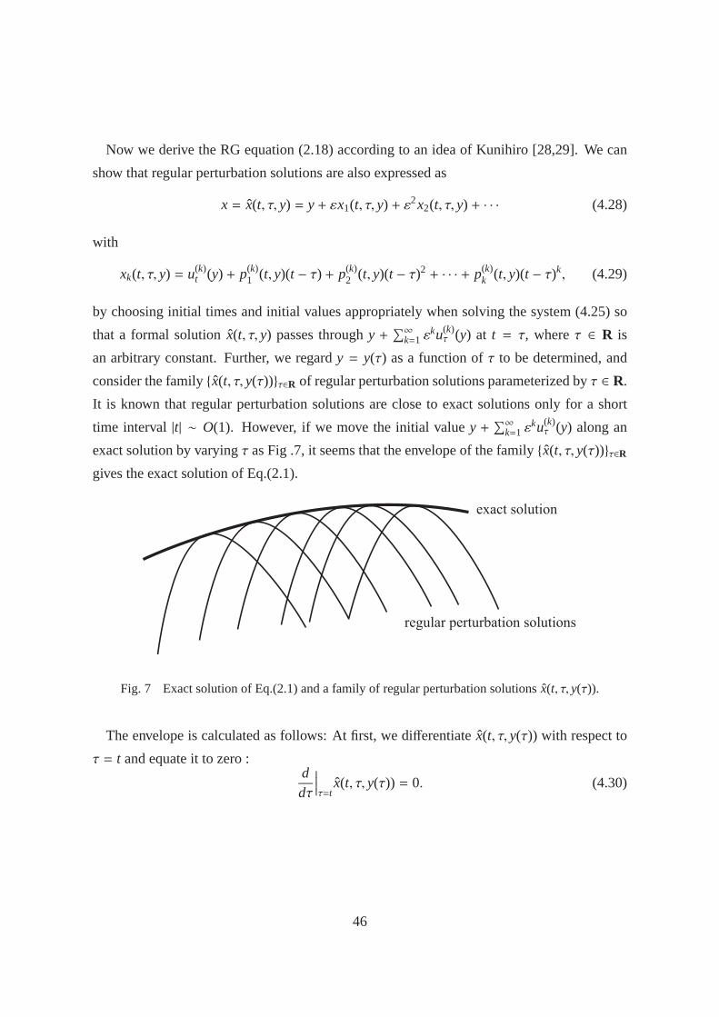
Now we derive the RG equation (2.18) according to an idea of Kunihiro [28,29]. We can

show that regular perturbation solutions are also expressed as

x = x(t, τ, y) = y + εx1(t, τ, y) + ε2x2(t, τ, y) + · · · (4.28)

with

xk(t, τ, y) = u(k)t (y) + p(k)

1 (t, y)(t − τ) + p(k)2 (t, y)(t − τ)2 + · · · + p(k)

k (t, y)(t − τ)k, (4.29)

by choosing initial times and initial values appropriately when solving the system (4.25) so

that a formal solution x(t, τ, y) passes through y +∑∞

k=1 εku(k)

τ (y) at t = τ, where τ ∈ R is

an arbitrary constant. Further, we regard y = y(τ) as a function of τ to be determined, and

consider the family {x(t, τ, y(τ))}τ∈R of regular perturbation solutions parameterized by τ ∈ R.

It is known that regular perturbation solutions are close to exact solutions only for a short

time interval |t| ∼ O(1). However, if we move the initial value y +∑∞

k=1 εku(k)

τ (y) along an

exact solution by varying τ as Fig .7, it seems that the envelope of the family {x(t, τ, y(τ))}τ∈Rgives the exact solution of Eq.(2.1).

exact solution

regular perturbation solutions

Fig. 7 Exact solution of Eq.(2.1) and a family of regular perturbation solutions x(t, τ, y(τ)).

The envelope is calculated as follows: At first, we differentiate x(t, τ, y(τ)) with respect to

τ = t and equate it to zero :ddτ

∣∣∣∣τ=t

x(t, τ, y(τ)) = 0. (4.30)

46

Substituting Eqs.(4.28) and (4.29) into the above yields

0 =dydt+

∞∑k=1

εk ddτ

∣∣∣∣τ=t

xk(t, τ, y(τ))

=dydt+

∞∑k=1

εk

∂u(k)t

∂y(y)

dydt− p(k)

1 (t, y)

=

dydt+

∞∑k=1

εk

∂u(k)t

∂y(y)

dydt− Rk(y) −

k−1∑j=1

∂u( j)t

∂y(y)Rk− j(y)

. (4.31)

This equality is formally satisfied if we define y = y(t) as a solution of the ODE

dydt=

∞∑k=1

εkRk(y). (4.32)

This recovers the m-th order RG equation if truncated at order εm. With this y(t), the envelope

for the family {x(t, τ, y(τ))}τ∈R is given by x(t, t, y(t)). Again Eqs.(4.28) and (4.29) prove that

x(t, t, y(t)) = y(t) +∞∑

k=1

εkxk(t, t, y(t))

= y(t) +∞∑

k=1

εku(k)t (y(t))

= α(m)t (y(t)) + O(εm+1), (4.33)

which gives the m-th order RG transformation if truncated at order εm.

In the rest of this section, we prove that a formal solution (4.24) with Eq.(4.26) obtained by

the regular perturbation method includes infinitely many convergent subseries even if Eq.(2.1)

(and thus Eq.(4.24)) is not analytic in ε.

Proposition 4.3. For sufficiently small |εt|, the series∑∞

l=1 εltl p(l+k)

l (t, y) are convergent for

k = 0, 1, 2, · · · .

To prove Prop.4.3, we need the next simple lemma.

Lemma 4.4. Let h1(t) and h2(t) be almost periodic functions with Mod(h1) ⊃ Mod(h2) (the

module of almost periodic functions is defined in Sec.2.1). If

limt→∞(h1(t) − h2(t)) = 0, (4.34)

then h1(t) = h2(t) for all t ∈ R.

47

Proof of Lemma 4.4. Functions hi, i = 1, 2 are expanded in Fourier series as hi(t) =∑λk∈Mod(h1) ci(λk)eiλkt. Then, Eq.(4.34) is rewritten as

limt→∞

∑λk∈Mod(h1)

(c1(λk) − c2(λk)) eiλkt = 0. (4.35)

This proves that c1(λk) = c2(λk) for all λk ∈ Mod(h1). �

Proof of Prop.4.3. Let

x(t) = y0 +

∞∑l=1

εltl p(l)l (y0) +

∞∑k=1

εk

u(k)t (y0) +

∞∑l=1

εltl p(l+k)l (t, y0)

(4.36)

be a formal solution of Eq.(2.1) constructed by the regular perturbation method and let y =

y(εt, ε) be a solution of the m-th order RG equation

dyd(εt)

= R1(y) + εR2(y) + · · · + εm−1Rm(y) (4.37)

for Eq.(2.1). By Thm.2.7, there exist positive constants C and T such that the inequality

||x(t) − α(m)t (y(εt, ε))|| < C|ε|m, 0 ≤ t ≤ T/ε (4.38)

holds if we choose initial values of x(t) and y(εt, ε) appropriately. Putting t = T/ε yields

α(m)T/ε(y(T, ε)) = y(T, ε) +

m∑k=1

εku(k)T/ε(y(T, ε))

= y0 +

∞∑l=1

T l p(l)l (y0) +

m−1∑k=1

εk

u(k)T/ε(y0) +

∞∑l=1

T l p(l+k)l (T/ε, y0)

+ O(εm). (4.39)

Note that functions u(k)t (y) and p(l+k)

l (t, y) are almost periodic functions in t such that Mod(u(k)t )

and Mod(p(l+k)l ) are included in Mod(g). In particular, they are bounded in t ∈ R. Thus taking

the limit ε→ 0 in Eq.(4.39) provides

y(T, 0) = y0 +

∞∑l=1

T l p(l)l (y0). (4.40)

This proves that the series∑∞

l=1 T l p(l)l (y0) is convergent.

Next thing to do is to prove Prop.4.3 for k = 1. Using Eq.(4.40) and dividing the both sides

of Eq.(4.39) by ε, we obtain

∞∑k=1

εk−1

k!∂ky

∂εk(T, 0)+

m∑k=1

εk−1u(k)T/ε(y(T, ε)) =

m−1∑k=1

εk−1

u(k)T/ε(y0) +

∞∑l=1

T l p(l+k)l (T/ε, y0)

+O(εm−1).

(4.41)

48

Taking the limit ε→ 0 yields

∂y∂ε

(T, 0) + limε→0

u(1)T/ε(y(T, 0)) − u(1)

T/ε(y0) −∞∑

l=1

T l p(l+1)l (T/ε, y0)

= 0. (4.42)

Now Lemma 4.4 proves that

∞∑l=1

T l p(l+1)l (t, y0) =

∂y∂ε

(T, 0) + u(1)t (y(T, 0)) − u(1)

t (y0), (4.43)

and the series∑∞

l=1 T l p(l+1)l (t, y0) proves to be convergent.

The proof of Prop.4.3 for k ≥ 2 is done in a similar way and omitted. �

Though it seems that Prop.4.3 has no relationship to the RG method, it is instructive to

notice the equality (4.40). Since y(T, 0) in the left hand side is obtained from a solution of

the first order RG equation dy/d(εt) = R1(y), the series∑∞

l=1 T l p(l)l (y0) proves to be deter-

mined by only the first order RG equation. This is remarkable because if we want to obtain∑∞l=1 T l p(l)

l (y0) by using the regular perturbation method, we have to solve infinitely many

ODEs (4,25). A similar argument shows that a solution of the m-th order RG equation in-

volves all terms of the form εk+ltl p(l+k)l (t, y0) for k = 0, · · · ,m − 1 and l = 1, 2, · · · in the

formal solution (4.24).

5 Infinite order RG equation

Infinite order RG equations and transformations are not convergent series in general. In this

section, we give a necessary and sufficient condition for the convergence. It will be proved

in Sec.5.3 that infinite order RG equations for linear systems are convergent and related to

Floquet theory.

5.1 Convergence condition

Let us consider the systemx = εg(t, x, ε), x ∈ M (5.1)

on a real analytic manifold M with the following assumption :

(A’) The vector field g is analytic with respect to t ∈ R, x ∈ M and ε ∈ I, where I ⊂ R is an

open interval containing 0. Further g is T -periodic in t.

49

Because of the periodicity, we can regard (5.1) as a system on S 1 × M :

ddt

(sx

)=

(1

εg(s, x, ε)

), (5.2)

where S 1 is a circle with a Cω structure.

Theorem 2.5 states that the infinite order RG transformation defined by

x = αt(y) := y + εu(1)t (y) + ε2u(2)

t (y) + · · · (5.3)

formally brings the system (5.1) into the infinite order RG equation

y = εR1(y) + ε2R2(y) + · · · , (5.4)

where “formally” means that Eqs.(5.3) and (5.4) are not convergent in general. If Eq.(5.3)

is convergent, so is Eq.(5.4). A necessary and sufficient condition for the convergence of

Eq.(5.3) is given as follows:

Theorem 5.1. For the system (5.1) with the assumption (A’), there exist an open neighbor-

hood U = Uy of S 1 × {y} × {0} in S 1 ×M × I for each y ∈ M and an analytic infinite order RG

transformation on U, if and only if the system (5.1) is invariant under the T1 (1-torus) action

of the formT

1 : (t, x) → (t + k, x + εσk(t, x, ε)), k ∈ R, (5.5)

where σk(t, x, ε) is analytic with respect to k, t, x, ε and T -periodic in k and t.

Recall that RG equations and RG transformations are not unique and not all of them are

convergent even if the condition of Thm.5.1 is satisfied.

The proof of this theorem involves Lie group theory and will be given in Sec.5.2, though

the idea of the proof is shown below.

Since the infinite order RG equation is an autonomous system, it is invariant under the

translation of t, (t, y) → (t + k, y). If an infinite order RG equation and transformation are

convergent and well-defined, the system (5.1) is invariant under the action defined by pulling

back the translation by the RG transformation :

(t, x) → (t + k, αt+k ◦ α−1t (x)). (5.6)

Since αt is T -periodic (Lemma 2.1 (ii)), this defines the T1 action on the space S 1 × M.

Conversely, if the system (5.1) is invariant under the action (5.5), then a simple extension

of Bochner’s linearization theorem proves that there exists a Cω coordinates transformation

x → y such that the action (5.5) is written as (t, y) → (t + k, y). We can show that this

50

transformation is just an RG transformation. See Section 5.2 for the detail.

In the rest of this subsection, we consider an autonomous system on Cn of the form

x = Fx + εg(x, ε)

= Fx + εg1(x) + ε2g2(x) + · · · , x ∈ Cn, (5.7)

with the assumptions (C1),(C2) (see Sec.2.1) and (C3) below :

(C3) g(x, ε) is analytic with respect to x ∈ Cn and ε ∈ I ⊂ R.

For this system, RG transformations are defined by Eq.(2.51) with Eqs.(2.46) to (2.49).

The next corollary immediately follows from Thm.5.1.

Corollary 5.2. Suppose that all eigenvalues of F have pairwise rational ratios. Then, there

exist an open neighborhood U = Uy of S 1 × {y} × {0} in S 1 × M × I for each y ∈ M and

an analytic infinite order RG transformation on U, if and only if the system (5.7) is invariant

under the T1 action of the form

T1 : x → eFkx + εσk(t, x, ε), k ∈ R, (5.8)

where σk(t, x, ε) is analytic with respect to k, t, x, ε and periodic in k and t.

Proof. By changing the coordinates as x = eFtX, Eq.(5.7) is rewritten as X = εe−Ftg(eFtX, ε).

Since eFt is periodic because of the assumption of Corollary 5.2, we can apply Thm.5.1 to

this system. Note that we do not need the assumption (C2) to prove Corollary 5.2. �

Recall that RG equations for Eq.(5.7) are equivalent to normal forms (Sec.4.3). If there are

irrational ratios among eigenvalues of F, Thm.5.1 is no longer applicable. For such a system,

Zung [54] gives a necessary and sufficient condition for the convergence of normal forms of

infinite order, although he supposes that gi(x) in Eq.(5.7) is a homogeneous vector field of

degree i for i = 2, 3, · · · . A necessary and sufficient condition for the convergence of infinite

RG equations and transformations for Eq.(5.7) is given in a similar way to Zung’s theorem as

follows:

Remember that an RG equation for Eq.(5.7) has the property that Ri(eFky) = eFkRi(y), k ∈R for i = 1, 2, · · · , if integral constants in Eqs.(2.47) and (2.49) are appropriately chosen

(Thm.2.15). If a matrix B satisfies the equalities FB = BF and Q(eBky) = eBkQ(y), k ∈ R

for all polynomial vector fields Q such that Q(eFky) = eFkQ(y), k ∈ R, then B is called

subordinate to F. It is known that if F is a diagonal matrix, we can take B having the form

51

B = diag (ib1, · · · , ibn), where i =√−1 and b j ∈ Z for j = 1, · · · , n (see Murdock [39], Zung

[54]). Let p be the maximum number of linearly independent such matrices B1, · · · , Bp and

call it the toric degree of F. Then, the matrix eB1k1+···+Bpkp , (k1, · · · , kp) ∈ Rp induces the Tp

action on Cn and the RG equation is invariant under this action. By a similar way to the proof

of Thm.5.1, we can prove the next theorem, whose proof is omitted here.

Theorem 5.3. Let p be the toric degree of F. For the system (5.7), there exist an open

neighborhood U = Uy of S 1 × {y} × {0} in S 1 × M × I for each y ∈ M and an analytic infinite

order RG transformation on U, if and only if (5.7) is invariant under the Tp action of the form

Tp : x → eB1k1+···+Bpkp x + εσk1,··· ,kp (t, x, ε), (k1, · · · , kp) ∈ Rp, (5.9)

where σk1,··· ,kp (t, x, ε) is analytic with respect to k1, · · · , kp, t, x, ε and periodic in k1, · · · , kp

and t.

5.2 Proof of Theorem 5.1

In this subsection, we give a proof of Thm.5.1. At first, we provide a few notations and

facts from Lie group theory.

Let K be a compact Lie group, dk a bi-invariant measure on K, V a complete locally

convex topological vector space, and π a representation of K in V . We define the average

av(π) : V → V of π by

av(π)(v) =∫

Kπ(k)(v)dk. (5.10)

Then, the next theorem holds (see Duistermaat and Kolk [15] for the proof).

Theorem 5.4. The average av(π) is a linear projection from V onto the space Vπ(K) := {v ∈V | π(k)v = v, ∀k ∈ K}; that is, equalities

π(k) ◦ av(π)(v) = av(π)(v) (5.11)

andav(π)(v) = v, v ∈ Vπ(K) (5.12)

hold.

Let S 1 be a circle with a Cω structure, M a real analytic manifold, and I ⊂ R an open

interval containing 0, as Sec.5.1. The next theorem is a simple extension of Bochner’s lin-

earization theorem [5,15].

52

Theorem 5.5. Let A : K → Diffω(S 1 × M × I) be a Cω action of K on S 1 × M × I such that

A(k) is expressed as

A(k)(t, x, ε) = (a1(k)(t), a2(k)(t, x, ε), ε), k ∈ K, (5.13)

where a1(k) : S 1 → S 1 and a2(k) : S 1 × M × I → M are Cω maps. Suppose that there exists

x0 ∈ M such thata2(k)(t, x0, 0) = x0. (5.14)

Then, there exist an open neighborhood U of S 1 × {x0} × {0} in S 1 × M × I and a Cω diffeo-

morphism ϕ from U into S 1 × Tx0 M × R such that

ϕ ◦ A(k) = (a1(k) × Dxa2(k)(t, x0, 0) × id) ◦ ϕ, (5.15)

where Dx is the derivative with respect to x. The ϕ is expressed as

ϕ(t, x, ε) = (t, a3(t, x, ε), ε) (5.16)

with a Cω map a3 and satisfies

ϕ(t, x0, 0) = (t, 0, 0), Dxϕ(t, x0, 0) = id. (5.17)

Further if we supposeDn

xa2(k)(t, x0, 0) = 0 (n ≥ 2), (5.18)

then ϕ satisfiesDn

xϕ(t, x0, 0) = 0 (n ≥ 2). (5.19)

Proof. Let W be a K-invariant open neighborhood of S 1 × {x0} × {0} and V a space of Cω

maps v : W → S 1 × Tx0 M × R such that

v(S 1 × {x0} × {0}) = S 1 × {x0} × {0}. (5.20)

Then V is a complete locally convex topological vector space.

Take a ϕ ∈ V expressed as

ϕ(t, x, ε) = (t, β(t, x, ε), ε) (5.21)

satisfyingDxβ(t, x0, 0) = id, Dn

xβ(t, x0, 0) = 0 (n ≥ 2), (5.22)

53

where β is a Cω map. Define the representation π of K in V to be

π(k)(v) = (a1(k) × Dxa2(k)(t, x0, 0) × id) ◦ v ◦ A(k)−1, (5.23)

and define ϕ ∈ V to be

ϕ = av(π)(ϕ) =∫

K(a1(k) × Dxa2(k)(t, x0, 0) × id) ◦ ϕ ◦ A(k)−1dk. (5.24)

Then Thm.5.4 implies that ϕ = π(k)(ϕ) and this proves Eq.(5.15). Eqs.(5.16),(5.17) and (5.19)

immediately follow from the definition (5.24) of ϕ with Eqs.(5.14),(5.18),(5.20),(5.21) and

(5.22). Since Dϕ(t, x0, 0) = id, ϕ is a Cω diffeomorphism on a neighborhood of S 1×{x0}×{0}by virtue of the inverse mapping theorem. �

Proof of Thm.5.1. Suppose that an infinite order RG transformation αt(y) is analytic in

U. Then, so is an infinite order RG equation. Since the RG equation is invariant under the

translation of t, Eq.(5.1) is invariant under the action defined by pulling back the translation

by the RG transformation:

(t, x) → (t + k, αt+k ◦ α−1t (x))

= (t + k, x + ε(u(1)t+k(x) − u(1)

t (x)) + O(ε2)), k ∈ R. (5.25)

Since αt is T -periodic, this defines the T1 action on S 1 × M of the form of (5.5).

Conversely, suppose that Eq.(5.1) is invariant under the T1 action (5.5). Let us rewrite

Eq.(5.1) as

ddt

sxε

=

1εg(s, x, ε)

0

. (5.26)

Then, the action (5.5) induces the action on S 1 × M × I of the form

A(k) : (s, x, ε) → (s + k, a2(k)(s, x, ε), ε), k ∈ R, (5.27)

where a2(k)(s, x, ε) = x + εσk(s, x, ε). Since a2(k) satisfies Eqs.(5.14) and (5.18) for any x ∈M, Thm.5.5 applies to show that there exist an open neighborhood U = Ux0 of S 1 × {x0} × {0}and a Cω diffeomorphism ϕ satisfying Eqs.(5.15) to (5.17) and (5.19) for each x0 ∈ M.

By taking a local coordinate near x0, we put x0 = 0 and identify a neighborhood of x0 with

a neighborhood of 0 in Tx0 M. Then, Eqs.(5.16), (5.17) and (5.19) prove that ϕ is expressed

asϕ(t, x, ε) = (t, x + εa3(t, x, ε), ε), (5.28)

54

where a3 is a Cω map. Thus ϕ defines the Cω transformation ψt by

x = ψt(y) = y + εa3(t, y, ε). (5.29)

Now Eq.(5.15) proves that if we transform Eq.(5.1) by x = ψt(y, ε), then the resultant equation

is invariant under the action

a1(k) × Dxa2(k)(t, x0, 0) × id : (t, x, ε) → (t + k, x, ε). (5.30)

Since this is the translation of t, the resultant equation has to be an autonomous system of the

formdydt= εR(y, ε), (5.31)

where R is analytic in y and ε.

Finally, we show that there exist an RG transformation and an RG equation which coincide

with Eqs.(5.29) and (5.31), respectively. Let Eqs.(5.3) and (5.4) be one of the RG transfor-

mations and the RG equations for Eq.(5.1), respectively. Since both of Eqs.(5.31) and (5.4)

are obtained from Eq.(5.1) by C∞ transformations ψt and αt, respectively, there exists an C∞

transformation φ which brings Eq.(5.31) into Eq.(5.4):

αt ◦ φ(y, ε) = ψt(y, ε). (5.32)

Because of Claim 2.16, there exists an RG transformation αt other than αt such that αt = αt◦φ.

This proves that there exists an analytic RG transformation αt = ψt. �

5.3 Infinite order RG equation for linear systems

In this subsection, we consider an n-dimensional linear system of the form

x = εA(t, ε)x, ,

= εA1(t)x + ε2A2(t)x + · · · , x ∈ Cn, (5.33)

where A(t, ε) is an n × n matrix. If this system satisfies the assumption (A), the RG method

is applicable. Since the RG equation and the RG transformation are linear in y ∈ Cn, it is

convenient to define matrices Ri and u(i)t to be

R1 = limt→∞

1t

∫ t

A1(s)ds, (5.34)

u(1)t =

∫ t

(A1(s) − R1) ds, (5.35)

55

and

Ri = limt→∞

1t

∫ t

i−1∑k=1

Ai−k(s)u(k)s + Ai(s) −

i−1∑k=1

u(k)s Ri−k

ds, (5.36)

u(i)t =

∫ t

i−1∑k=1

Ai−k(s)u(k)s + Ai(s) −

i−1∑k=1

u(k)s Ri−k − Ri

ds, (5.37)

for i = 2, 3, · · · , respectively. With these matrices, the m-th order RG equation and the m-th

order RG transformation for Eq.(5.33) are defined by

y = εR1y + ε2R2y + · · · + εmRmy, y ∈ Cn, (5.38)

α(m)t y = y + εu(1)

t y + · · · + εmu(m)t y, y ∈ Cn, (5.39)

respectively. Since the RG equation is a linear system with a constant coefficient, we can

easily determine the stability of the trivial solution x = 0 of Eq.(5.33) by using the RG

equation. See Chiba [11] for the detail.

In what follows, we suppose the following assumption :

(L) The matrix A(t, ε) is T -periodic in t and analytic with respect to ε ∈ D, where D ⊂ C is

an open neighborhood of the origin.

Let us consider the infinite order RG equation y =∑∞

k=1 εkRky := R(ε)y and the infinite

order RG transformation αty = y +∑∞

k=1 εku(k)

t y. Then, the fundamental matrix X(t, ε) of

Eq.(5.33) is given byX(t, ε) = αt · eR(ε)t. (5.40)

An initial value is given by X(0, ε) = α0 = id +∑∞

k=1 εku(k)

0 and it can be taken arbitrarily

by choosing integral constants in Eqs.(5.35) and (5.37) appropriately. We suppose that the

integral constants are chosen so that an initial value α0 is analytic in ε ∈ D. Then, X(t, ε) is

analytic in ε ∈ D. Now the question arises whether αt and R(ε) are analytic in ε.

Theorem 5.6. Suppose that Eq.(5.33) satisfies the assumption (L) and α0 is chosen to be

analytic in ε ∈ D. Then, there exists a positive number r0 such that R(ε), eR(ε)t and αt are

analytic on the disk |ε| < r0.

Proof. Since αt is T -periodic (Lemma 2.1 (ii)), the equality

X(t + T, ε) = αt+T · eR(ε)(t+T )

= αt · eR(ε)t · eR(ε)T

= X(t, ε) · eR(ε)T (5.41)

56

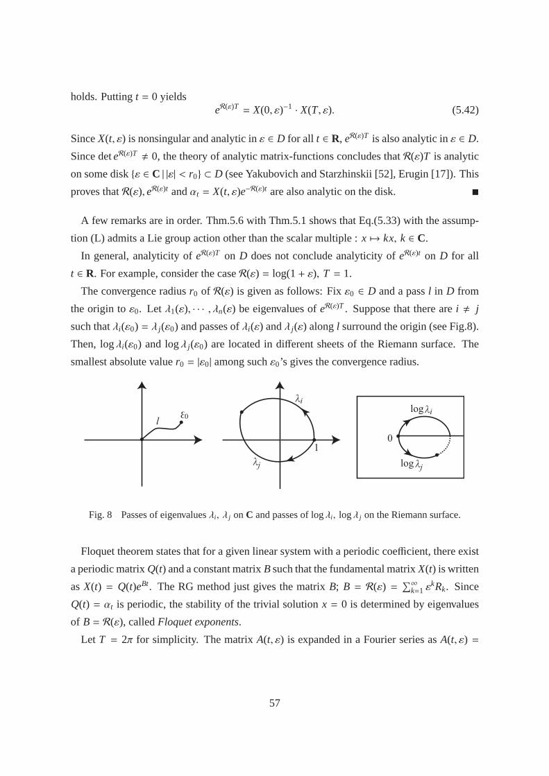
holds. Putting t = 0 yieldseR(ε)T = X(0, ε)−1 · X(T, ε). (5.42)

Since X(t, ε) is nonsingular and analytic in ε ∈ D for all t ∈ R, eR(ε)T is also analytic in ε ∈ D.

Since det eR(ε)T � 0, the theory of analytic matrix-functions concludes that R(ε)T is analytic

on some disk {ε ∈ C | |ε| < r0} ⊂ D (see Yakubovich and Starzhinskii [52], Erugin [17]). This

proves that R(ε), eR(ε)t and αt = X(t, ε)e−R(ε)t are also analytic on the disk. �

A few remarks are in order. Thm.5.6 with Thm.5.1 shows that Eq.(5.33) with the assump-

tion (L) admits a Lie group action other than the scalar multiple : x → kx, k ∈ C.

In general, analyticity of eR(ε)T on D does not conclude analyticity of eR(ε)t on D for all

t ∈ R. For example, consider the case R(ε) = log(1 + ε), T = 1.

The convergence radius r0 of R(ε) is given as follows: Fix ε0 ∈ D and a pass l in D from

the origin to ε0. Let λ1(ε), · · · , λn(ε) be eigenvalues of eR(ε)T . Suppose that there are i � j

such that λi(ε0) = λ j(ε0) and passes of λi(ε) and λ j(ε) along l surround the origin (see Fig.8).

Then, log λi(ε0) and log λ j(ε0) are located in different sheets of the Riemann surface. The

smallest absolute value r0 = |ε0| among such ε0’s gives the convergence radius.

Fig. 8 Passes of eigenvalues λi, λ j on C and passes of log λi, log λ j on the Riemann surface.

Floquet theorem states that for a given linear system with a periodic coefficient, there exist

a periodic matrix Q(t) and a constant matrix B such that the fundamental matrix X(t) is written

as X(t) = Q(t)eBt. The RG method just gives the matrix B; B = R(ε) =∑∞

k=1 εkRk. Since

Q(t) = αt is periodic, the stability of the trivial solution x = 0 is determined by eigenvalues

of B = R(ε), called Floquet exponents.

Let T = 2π for simplicity. The matrix A(t, ε) is expanded in a Fourier series as A(t, ε) =

57

∑+∞−∞ cn(ε)eint. By changing the independent variables as z = eint, Eq.(5.33) is written as

dxdz= −iε

+∞∑−∞

cn(ε)zn−1x. (5.43)

This is a linear system on a complex domain having the singularity at the origin. It is known

that the fundamental matrix of this system is expressed as

X(z) = S (z) · eM·log z, (5.44)

where S (z) is a single-valued matrix and M = M(ε) is a constant matrix called monodromy

matrix. It is easy to verify that R(ε) = iM and the RG method provides the monodromy

matrix.

Acknowledgments

The author would like to thank Professor Toshihiro Iwai for critical reading of the manu-

script and for useful comments.

References

[1] L. Arnold et al, Dynamical systems, Lecture notes in mathematics 1609, SpringerVerlag, 1995

[2] G. Belitskii, C∞-normal forms of local vector fields, Acta Appl. Math. 70 (2002), no.1-3, 23–41

[3] C. M. Bender, S. A. Orszag, Advanced mathematical methods for scientists and engi-neers, McGraw-Hill Book Co., New York, 1978

[4] I. I. Blekhman, Synchronization in Science and Technology, ASME press, 1988[5] S. Bochner, Compact groups of differentiable transformations, Ann. of Math. (2) 46,

(1945). 372–381[6] N. N. Bogoliubov, Y. A. Mitropolsky, Asymptotic methods in the theory of non-linear

oscillations, Hindustan Publishing Corp., Delhi, Gordon and Breach Science Publish-ers, New York 1961

[7] J. Carr, Applications of Centre Manifold Theory, Springer-Verlag, 1981[8] L. Y. Chen, N. Goldenfeld, Y. Oono, Renormalization group theory for global asymp-

totic analysis, Phys. Rev. Lett. 73 (1994), no. 10, 1311-15[9] L. Y. Chen, N .Goldenfeld, Y. Oono, Renormalization group and singular perturba-

tions: Multiple scales, boundary layers, and reductive perturbation theory, Phys. Rev.E 54, (1996), 376-394

[10] H. Chiba, C1 approximation of vector fields based on the renormalization groupmethod, SIAM J. Appl. Dym. Syst., Vol.7, No.3, (2008) 895–932

[11] H. Chiba, Simplified Renormalization Group Equations for Ordinary DifferentialEquations, J. Differ. Equ. 246, (2009) 1991-2019

58

[12] H. Chiba, Approximation of Center Manifolds on the Renormalization Group Method,J. Math. Phys. Vol.49, 102703 (2008).

[13] H. Chiba, D. Pazo, Stability of an [N/2]-dimensional invariant torus in the Kuramotomodel at small coupling, Physica D, (in press)

[14] S. N. Chow, C. Li, D. Wang, Normal forms and bifurcation of planar vector fields,Cambridge University Press, 1994

[15] J. J. Duistermaat, J. A. C. Kolk, Lie groups, Universitext. Springer-Verlag, Berlin,2000

[16] S. Ei, K. Fujii, T. Kunihiro, Renormalization-group method for reduction of evolutionequations; invariant manifolds and envelopes, Ann. Physics 280 (2000), no. 2, 236-298

[17] N. P. Erugin, Linear systems of ordinary differential equations with periodic and quasi-periodic coefficients, Academic Press, New York-London, 1966

[18] N. Fenichel, Persistence and smoothness of invariant manifolds for flows, IndianaUniv. Math. J., 21(1971), pp. 193-226

[19] N. Fenichel, Geometric singular perturbation theory for ordinary differential equa-tions, J. Differential Equations 31 (1979), no.1, pp.53-98

[20] A. M. Fink, Almost periodic differential equations, Lecture Notes in Mathematics,Vol. 377. Springer-Verlag, Berlin-New York, 1974

[21] S. Goto, Renormalization Reductions for Systems with Delay, Prog. Theor. Phys.118. No.2 (2007), 211–227

[22] S. Goto, Y. Masutomi, K. Nozaki, Lie-Group Approach to Perturbative Renormaliza-tion Group Method, Progr. Theoret. Phys., vol.102, No.3.(1999), pp. 471-497.

[23] W. Hahn, Stability of motion, Springer-Verlag New York, 1967[24] M.W. Hirsch, C.C. Pugh, M. Shub, Invariant manifolds, Springer-Verlag, 1977, Lec.

Notes in Math., 583[25] F.C. Hoppensteadt, E.M. Izhikevich, Weakly connected neural networks, Springer-

Verlag, New York, 1997[26] E. Kirkinis, On the Reduction of Amplitude Equations by the Renormalization Group

Approach, Phys. Rev. E, (1) 77, 2008[27] E. Kirkinis, The Renormalization Group and the Implicit Function Theorem for Am-

plitude Equations, J. Math. Phys. (7), 49, 2008[28] T. Kunihiro, A geometrical formulation of the renormalization group method for

global analysis, Progr. Theoret. Phys. 94 (1995), no. 4, 503-514[29] T. Kunihiro, The renormalization-group method applied to asymptotic analysis of vec-

tor fields, Progr. Theoret. Phys. 97 (1997), no. 2, 179-200[30] T. Kunihiro, J. Matsukidaira, Dynamical reduction of discrete systems based on the

renormalization-group method, Phys. Rev. E. Vol.57, No.4, 4817–4820, 1998[31] T. Kunihiro, K. Tsumura, Application of the renormalization-group method to the

reduction of transport equations, J. Phys. A 39 (2006), no.25, 8089–8104[32] R. E. Lee DeVille, A. Harkin, M. Holzer, K. Josic, T. Kaper, Analysis of a renor-

malization group method and normal form theory for perturbed ordinary differentialequations, Physica D, (2008)

[33] I.G. Malkin, The Methods of Lyapunov and Poincare in the Theory of Nonlinear Os-

59

cillations, Moscow-Leningrad, 1949[34] I.G. Malkin, Some problems of the theory of nonlinear oscillations, Gosudarstv. Izdat.

Tehn.-Teor. Lit., Moscow, 1956[35] B. Mudavanhu, R.E. O’Malley Jr., A new renormalization method for the asymptotic

solution of weakly nonlinear vector systems, SIAM J. Appl. Math. 63 (2002), no.2,373–397

[36] B. Mudavanhu, R.E. O’Malley Jr., A renormalization group method for nonlinear os-cillators, Stud. Appl. Math. 107 (2001), no. 1, 63–79

[37] J. Murdock, Frequency entrainment for almost periodic evolution equations, Proc.Amer. Math. Soc. 96 (1986), no. 4, 626–628

[38] J. Murdock, Perturbations. Theory and methods, John Wiley & Sons, Inc., New York,1991

[39] J. Murdock, Normal forms and unfoldings for local dynamical systems, Springer-Verlag, New York, (2003)

[40] J. Murdock, Hypernormal form theory: foundations and algorithms, J. DifferentialEquations, 205 (2004), no. 2, 424-465

[41] J. Murdock, L.C. Wang, Validity of the multiple scale method for very long intervals,Z. Angew. Math. Phys. 47 (1996), no. 5, 760–789

[42] S. Murata, K. Nozaki, Renormalization group symmetry method and gas dynamics,Internat. J. Non-Linear Mech. 39 (2004), no. 6, 963–967

[43] A. H. Nayfeh, Method of Normal Forms, John Wiley & Sons, INC., 1993[44] A. H. Nayfeh, Introduction to perturbation techniques, John Wiley & Sons, New York,

1981[45] K. Nozaki, Y. Oono, Renormalization-group theoretical reduction, Phys. Rev. E,

63(2001), 046101[46] K. Nozaki, Y. Oono, Y. Shiwa, Reductive use of renormalization group, Phys. Rev. E

(3) 62 (2000), no. 4, 4501–4504[47] J.A. Sanders, F. Verhulst, J. Murdock, Averaging methods in nonlinear dynamical

systems, Springer, New York, 2007[48] T. Tsumura, T. Kunihiro, K. Ohnishi, Derivation of covariant dissipative fluid dynam-

ics in the renormalization-group method, Phys. Lett. B 646 (2007), no. 2-3, 134–140.[49] S.I. Tzenov, R.C. Davidson, Renormalization group reduction of the Henon map and

application to the transverse betatron motion in cyclic accelerators, New J. Phys. 5(2003), 67.1–67.13

[50] F. Verhulst, Methods and applications of singular perturbations. Boundary layers andmultiple timescale dynamics, Texts in Applied Mathematics, 50. Springer, New York,(2005)

[51] S. Wiggins, Normally hyperbolic invariant manifolds in dynamical systems , Springer-Verlag, 1994

[52] V. A. Yakubovich, V. M. Starzhinskii, Linear differential equations with periodic co-efficients 1, John Wiley & Sons, New York-Toronto, 1975

[53] M. Ziane, On a certain renormalization group method, J. Math. Phys. 41 (2000), no.5, 3290-3299

[54] N. T. Zung, Convergence versus integrability in Poincare-Dulac normal form, Math.

60

Res. Lett. 9 (2002), no. 2-3, 217–228[55] I. Moise, R. Temam, Renormalization group method. Application to Navier-Stokes

equation, Discrete Contin. Dynam. Systems 6 (2000), no. 1, 191–210[56] I. Moise, M. Ziane, Renormalization group method. Applications to partial differential

equations, J. Dynam. Differential Equations 13 (2001), no. 2, 275–321[57] M. Petcu, R. Temam, D. Wirosoetisno, Renormalization group method applied to the

primitive equations, J. Differential Equations 208 (2005), no. 1, 215–257[58] Y. Shiwa, Renormalization-group theoretical reduction of the Swift-Hohenberg model,

Phys. Rev. E 63, 016119 (2000)[59] Tao. Tu, G. Cheng, Renormalization group theory for perturbed evolution equations,

Phys. Rev. E (3) 66 (2002), no. 4, 046625

61