Nonlrnwr Anolysrs, Theory, Melhods d Applicarrons, Vol. 15, No. 5. pp. 467-478. 1990. 0362-546X/90 $3.00+ .OO Prmted I” Great Brnam. :C 1990 Pergamon Press plc

ON NONLINEAR SINGULAR PERTURBATION PROBLEMS

PHILIP KORMAN

Department of Mathematical Sciences, University of Cincinnati, Cincinnati, OH 45221-0025, U.S.A.

(Received 23 July 1989; received for publication 26 February 1990)

Key words and phruses: Singular perturbation problems, existence of solutions, a priori estimates.

1. INTRODUCTION

IN THIS paper we consider two types of singular perturbation problems. In the first part we con- sider boundary value problems of the type

Au = &j-(x, u, Du, D’u, D3u) o<x,< 1, u(x’, 0) = U(X’, 1) = 0. (1.1)

Here u = u(x), x = (x’,x,,), x’ E T”-‘, 0 I x, i 1, where T”-’ is the n - 1 dimensional torus (say T”-’ = [0, 27rln-‘), Du, D’u, D3u denote all derivatives of u of orders one, two and three. Our work was motivated by the papers of Rabinowitz [5, 61 and Kato [l], who considered the equation (1.1) on the torus T” (no boundary conditions), and established existence of solutions for sufficiently small E. Rabinowitz used the Nash-Moser technique, while Kato was using his abstract results on coercive mappings. Both approaches made use of a priori estimates in high order Sobolev spaces for either (1 .l) or its linearized version. Such estimates involve differentiation of the equation, after which the boundary conditions are in general lost, and hence the results of [ 1,5,6] were restricted to the torus. We show that for the strip-like domains some apriori estimates and existence results are possible. Naturally, our conditions on the non- linear term f are far more restrictive than those of Rabinowitz [5], in particular we allow only those third order terms which are either of the type uXiXjXn or uXIXj_. with 1 5 i,j, k I n - 1.

In the second part we consider equations on the torus. In [l], to prove existence, Kato was deriving a priori estimates for fully nonlinear equations, which are rather involved. In Section 5 we show that in order to apply the abstract result of Kato it essentially suffices to derive a priori estimates for the linearized equation, which is easier. As an application we extend a well-known result of Moser [4].

Next we discuss the notation and state some preliminary results. We consider functions on the domain V = T”-’ x [0, 11. We shall abbreviate If = jVf,

and in Section 5, jf = lrnf. We assume that the Roman letters i, j, k, . . . , run from 1 to n - 1, while the Greek CY, p, y, . . . , from 1 to n and denote Ui = (aU/aXi), U;jol = (83U/8Xiaxjax,), etc. Summation on repeated indices (as in (2.1)) is implied. By 11. Ilrn we denote the mth Sobolev norm in V. We shall also need the norms (in I/or T”)

We shall denote

If1, = ,& IDaft,-, m = integer 2 0.

6, = max Ibij,l,.

i,j,u

467

468 P. KORMAN

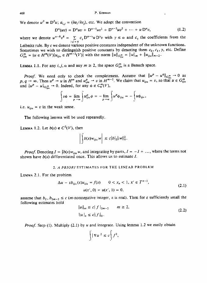
We denote u8 = DBu; ai,i = (aa;/aXj), etc. We adopt the convention

D”(uu) = D’%u + D”-‘uu’ + Da-‘uu2 + . -. + u D%, (1.2)

where we denote zYkuk = 1 crD a-Yu DYu with y 5 CY and cr the coefficients from the IYI =k

Leibnitz rule. By c we denote various positive constants independent of the unknown functions. Sometimes we wish to distinguish positive constants by denoting them co, cl, y, etc. Define G;a = (U E H”(V)Iuij, E ZYm-2(V)) with the norm IIuII~.v_ = ll~ll,,, + IJU;juIlm-2*

LEMMA 1.1. For any i,j, CY and any m L 2, the space G& is a Banach space.

Proof. We need only to check the completeness. Assume that llup - u4110;= + 0 as p, q + co. Then up --, u in H” and u& --i u in Hmw2. We claim that Uiju = U, SO that u E Grf

and /Iup - ~l(o;~ -+ 0. Indeed, for any 4~ E C,“(V),

i.e. Uija = u in the weak sense.

The following lemma will be used repeatedly.

LEMMA 1.2. Let b(x) E C2( V), then

/ ~NX1WijaWi 5 cIbI2IIwII:*

Proof. Denoting Z = Sb(X)Wij, w, and integrating by parts, Z = -Z + . . . , where the terms not shown have b(x) differentiated once. This allows us to estimate I.

2. A PRIORI ESTIMATES FOR THE LINEAR PROBLEM

LEMMA 2.1. For the problem

AU - Eb;ja(X)Uija =_f(X) 0 < x, < 1, x’ E T”-I, (2.1)

u(x’, 0) = u(x’, 1) = 0,

assume that b2, b2,_2 I c (m-nonnegative integer, E is real). Then for E sufficiently small the following estimates hold

l14m 5 Cllfllzm-2 m 2 2, (2.2)

ll4l 5 dfllo.

Proof. Step (1). Multiply (2.1) by u and integrate. Using lemma 1.2 we easily obtain

Nonlinear singular perturbation problems 469

provided bz I c, which proves (2.2) for M = 1. Next, we multiply (2.1) by ukk and integrate. Similarly,

‘;$J j vu,12 I c f2. (2.3)

To finish the estimation of 11~11: we need a bound on ju&. When expressed from (2.1), u,, depends on the third order terms, not yet estimated. This leads us to differentiate (2.1) in the tangential directions.

AukI - Ebijauijakl - Ebija,kUijaI - Ebijm,/Uijctk - &bija,klUija = fkl- (2.4)

Multiply (2.4) by uk/ and integrate. Since by lemma 1.2 (integrating by parts in Xi, Xj and x,)

1 Sbija~ijczk,uk,l 5 Cb2 kI$ 1 1 I VUklI’, (2.5)

we obtain (for sufficiently small E)

k;$l 1’ 1 v&l2 5 c f;,.

Expressing now u,, from the equation (2.1), and using (2.6) we estimate

(2.6)

which together with (2.6) gives us the estimate (2.2) for m = 2.

Step (2). To get higher order estimates we differentiate the equation and proceed similarly. Let multi-index /3 = (p’, 0) with IpI = m - 1, and denote u’ = D%. Differentiate the equation (2.1) (and use the notation described previously), and then multiply by u’ and integrate,

Using lemma 1.2 on the second term on the left, and summing on all /I with B,, = 0, we easily obtain

Q vuS12 5 cllf IIL, assuming b,_l -c c. (2.7)

P

Next we need to estimate the derivatives of order m, where more than one derivative in x,, is allowed. Let now fl = (j?‘, 0) with I/III = m - k. We shall prove that

s (Dyk~‘)~ 5 cllf ltz+k-2 3 assuming bm+k_2 5 c, (2.8)

using induction on k 2 2. Let k = 2, I/3 = m - 2. Express u,, from the equation (2.1) and differentiate,

n-l Ua = - C Us + Ebijolu~or + Eb!. UP-’ + ... + Eb~,uij, + fS. nn ,,o[ ,,a

i=l

470 P. KORMAN

Applying (2.7) (with IpI + 2 = m, yn = 0),

~(u!,J2’r c(ll_fll~_~ + ,zrn jl~d~) 5 cllfllK, provided 6, 5 c.

Assuming (2.8) to be true for k we now prove it for k + 1 (with IpI = m - k - 1). Differentiating the equation (2-l),

n-1

D;r+‘uO = - c D;-‘u{ + ebij,D;-‘u;, + . . . + 0,“-‘f4, i=l

where .a. denotes the lower order terms. The second term on the right involves a derivative of u of order m + 1, which includes up to k differentiations in x,, . Applying (2.8), we obtain

”

?

(D:+‘u‘?~ 5 cllfllk+,-1, assuming bm+k_l I c.

(By (2.8) when estimating j(u’)’ all that matters is IyI and y,.) From the estimates (2.8) the lemma follows.

This lemma can be used to give existence and uniqueness results for the problem (2.1). We start with the simplest one.

THEOREM 2.1. Assume that all b,, are constants, and Ilf(12m_2 I c for m 2 1. Then for E suffi- ciently small the problem (2.1) has a unique solution of class H”‘.

Proof. Look for the solution in the form u(x) = CI u,(x,)e”‘X’, with 1 = (II, . . . , I,_,). Then from (2.1), writing, f = C,fr(x,)e”‘“‘,

u;l - III’u, - Eib;jkliljlk~I - Eb;jnliljUi = fj(X,)

(2.9) u,(O) = U[(l) = 0.

We claim that (2.9) is uniquely solvable for all multi-indices 1. Then the proof will follow, since lemma 1.2 will imply convergence of the series Cu,(x,)e” ’ ” and the regularity. To prove the claim, write u,(x) = u(x) + iw(x) with real u and w. Then for the adjoint equation to (2.9)

u” - (II’u + EbijnliIjU’ + EbijkliljlkW = Refr(x,,)

W” - 1f12w + EbUnliljW - Ebijkli[il~U = Imf,(x,,) (2.10)

u(0) = V(1) = w(0) = w(1) = 0.

Assume for the moment that f,(x,,) = 0. Then multiplying the first equation in (2.10) by u, the second one by w, adding and integrating by parts,

1

1

(?P + 1112v2 + wf2 + ~/~2w2)cLxn = 0,

,O

i.e. V(X,,) = w(x,,) = 0. Applying the Fredholm alternative we get the solvability of (2.9).

” ._,.._._. _. . . ^ -._.__.-. “..l-.- _ _. . .._. ._ . _ _.__-“- _..-

Nonlinear singular perturbation problems 471

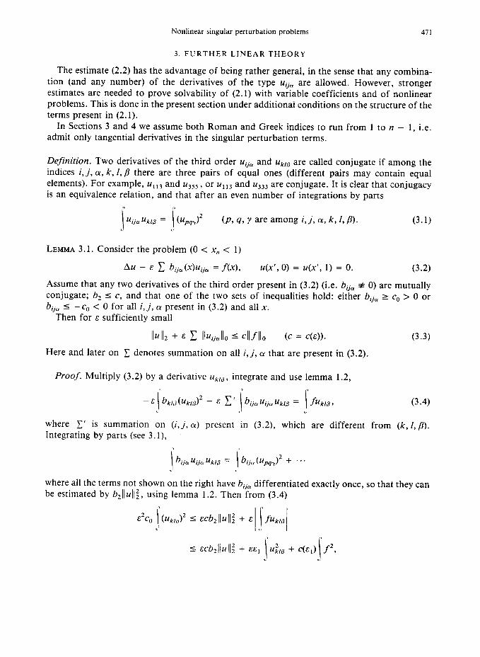
3. FURTHER LINEAR THEORY

The estimate (2.2) has the advantage of being rather general, in the sense that any combina- tion (and any number) of the derivatives of the type Uij,, are allowed. However, stronger estimates are needed to prove solvability of (2.1) with variable coefficients and of nonlinear problems. This is done in the present section under additionai conditions on the structure of the terms present in (2.1).

In Sections 3 and 4 we assume both Roman and Greek indices to run from 1 to n - 1, i.e. admit only tangential derivatives in the singular perturbation terms.

Definition. TWO derivatives of the third order Uije and uklB are called conjugate if among the indices i, j, CY, k, I, /I there are three pairs of equal ones (different pairs may contain equal elements). For example, u1i3 and uJS5, or u1i3 and u333 are conjugate. It is clear that conjugacy is an equivalence relation, and that after an even number of integrations by parts

,

I

n

uijm Uklp =

<I I h7J2 (A 4, Y are among i, j, a, k, L/3). (3.1)

<>

LEMMA 3.1. Consider the problem (0 < x, < 1)

AU - s C b;j, (X)Uij, = f(X), U(X’, 0) = u(x’, 1) = 0. (3.2)

Assume that any two derivatives of the third order present in (3.2) (i.e. bij, f 0) are mutually conjugate; bz I c, and that one of the two sets of inequalities hold: either bij, 2 co > 0 or 6,, I - c, < 0 for all i, j, (Y present in (3.2) and all x.

Then for E sufficiently small

Ilull + & C IIUijal10 s cllfl10 (c = C(E)). (3.3)

Here and later on C denotes summation on all i, j, 01 that are present in (3.2).

Proof. Multiply (3.2) by a derivative uk[4, integrate and use lemma 1.2, 1 > 1

- & b,,&k,d2 - I & 1’ bijauija Uklf3 = fUk&Y Y

c ,I / I

(3.4)

where C’ is summation on (i, j, a) present in (3.2), which are different from (k, I, 8). Integrating by parts (see 3.1)

where all the terms not shown on the right have b,, differentiated exactly once, so that they can be estimated by b211ul\i, using lemma 1.2. Then from (3.4)

,>

f-‘9

472 P. KORMAN

so that by choosing cl small, we estimate

Next, we multiply (3.2) by u,+, integrate by parts using lemma 1.2, and sum

*? jl VUk12 I C&llf# + C(E) f2. k=l r c

Expressing u,,, from the equation (3.2), and using (3.5)-(3.6),

(3.5)

(3.6)

(3.7)

Adding (3.5-3.7) we conclude the lemma.

THEOREM 3.1. In the conditions of lemma 3.1, with b,, E L”(V) for all i, j, a, the problem (3.2) is solvable for sufficiently small E, i.e. for every f l L2( V) there is a unique u E ni,j,, G&(V) = G solving (3.2).

Proof. Assume for definiteness that b,, L co for all i, j, a and all x. Consider an auxiliary problem

AM - E C CoUij~ = f(X), u(x’, 0) = u(x’, 1) = 0. (3.8)

As in the theorem 2.1, we can write a Fourier series solution for (3.8), which by the estimate (3.3) converges and belongs to G. Next, for 0 5 t I 1 we consider a family of problems

AU - E C [co(l - t) + tbij,]Uij, = f(X), u(x',O) = u(x', 1) = 0. (3.9)

Denote S = (1 E [0, l] I (3.9) has a solution of class G). Clearly, 0 E S. We shall show that S is both open and closed in [0, 11.

(i) Openness. Assume to E S. Define a map T, u = Tii, by solving

AU - E C [cO(I - to) + tobij,(X)]Uij, = f

- E c [-co(t0 - t) + (to - t)b;ja(x)la,a,

with u(x’, 0) = u(x’, 1) = 0. The estimate 3.3 implies that T takes G into itself, and is a contraction for It - toI small.

(ii) Closedness. Assume there is a sequence It,], such that t, E S and t, + ?as n -+ 43. Let U” be solution of (3.9) corresponding to t,. By (3.3), it follows that ll~“]]~, IIu~~IJ~ s c for all i,j, a, so that without loss of generality we may assume that U” - ii in H*(u), ucn - u in L*(V). We claim that u = iiija, so that u E G& . Indeed, letting @I E C,“(V),

Passing to the limit in (3.9), we obtain that ?E S. (Multiplying (3.9) by a test function 4, we can first pass to the limit in the integral form, and then conclude (3.9), since 4 is arbitrary.)

In the next result the singular perturbation terms need not be small.

Nonlinear singular perturbation problems

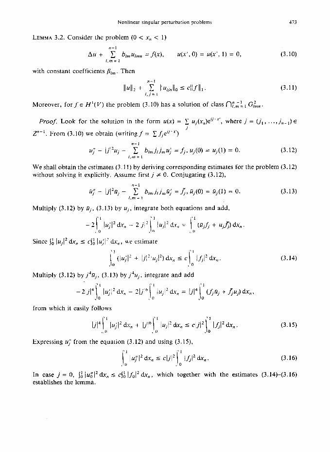
LEMMA 3.2. Consider the problem (0 < x, < 1)

n- 1

Au + c b,, U,n,n = f(x), u(x’, 0) = u(x’, 1) = 0, /.m=l

473

(3.10)

with constant coefficients Bin,. Then

n-l

Ilull + C IIz4ijnl10 5 cllfIIl. (3.11) i,j=l

Moreover, for f E Zf’( V) the problem (3.10) has a solution of class f-l!,: 1 GA,,.

Proof. Look for the solution in the form U(X) = 1 uj(x,)eij’“‘, where j = (ji , . . ., j,_r) E i

Z”-‘. From (3.10) we obtain (writing f = C&e’/‘“‘)

n-1

u;’ - JjJ’Uj - 1 bimj,jmU/I =f,, ~j(0) = Uj(l) = 0. (3.12) 1,m = I

We shall obtain the estimates (3.1 I) by deriving corresponding estimates for the problem (3.12) without solving it explicitly. Assume first j # 0. Conjugating (3.12),

n-l DT - Ij12ii, - C b[,,,j,j,,,aj = A, ~j(0) = ~j(l) = 0. (3.13)

I.m= 1

Multiply (3.12) by iij, (3.13) by u, , integrate both equations and add,

Since 1; IujJ* dx, I cjh lz4ilz dx,, we estimate

\ ’ (izc;l’ + ljj'jz4,12)dx,, 5 c .I0

I o Ifjl’ tin. I

Multiply (3.12) by j4c,, (3.13) by j”u.j, integrate and add

-4A4 Ld l~,!l~ti,, - 21jl"['lUj12d~, = lj14['(&uj +Ju~)~x,,, i .O .O

from which it easily follows

(3.14)

(3.15)

Expressing u;’ from the equation (3.12) and using (3.19,

it: iup dx, 5 dd2 id iby dx,. ,a

(3.16)

In case j = 0, {A lu$ I* dx, 5 cJA j fo12 dx,, which together with the estimates (3.14)-(3.16) establishes the lemma.

414 P. KORMAN

Remark 3.1. We discuss here the third order terms, which were not present in the lemmas 2.1 and 3.1. It appears that the term u,,,, cannot be allowed as the following simple example shows. The problem

Au - au,,,, = 0 0 < x, < 1, x’ E T”-’

u(x’, 0) = 24(x’, 1) = 0,

has a nontrivial solution u = e”‘E)xn - (e”’ - 1)x, - 1, so that no a priori estimate like (2.2) or (3.3) is possible. However, the terms of the type u,,,~ can be included under some conditions. For example, let u(x, y) be solution of (a = const)

u, + uuv + auqy = f(x, Y) O<y< l,x~T’,

u(x, 0) = u(x, 1) = 0.

Using the Fourier series analysis one derives an estimate

(3.17)

which can be used to prove existence of solution.

4. NONLINEAR BOUNDARY VALUE PROBLEMS

THEOREM 4.1. Consider the problem

AU - E C bij,(X)Uij, = 6f(X, U, Du, D*u, Uij,) o<x,< 1,

u(x’, 0) = u(x’, 1) = 0, x’ E T”-‘. (4.1)

Assume that the coefficients 61, satisfy all conditions of the theorem 3.1, while the function f depends only on those third order derivatives that are present on the left in (4.1), f is of class C’ and satisfies

Ifl 5 c(l + l”l + C lull + C I”ijI + C l”ijal)v (4.1)

IfA IL,L Ifu,,19 k,,.,l 5 ,“I i,j.u

for all i, j, o, (4.2)

for all values of its arguments. Then for E and 6 sufficiently small (6 = B(E)) the problem (4.1) has a solution of class G (G was defined in the theorem 3.1).

Proof. Define a map T, u = TV by solving

AU - E C bi,,Uij, = 6f(X, V, Dv, D2tl, Vij,) 0 < x, < 1, u(x’, 0) = u(x’, 1) = 0.

By the theorem 3.1, for v E G the map T is well-defined, and takes G into itself. Using the mean value theorem, one easily shows that T is a contraction.

Further nonlinear existence results can be stated, based on the estimates (3.11) and (3.17).

5. QUASILINEAR SECOND ORDER EQUATIONS ON A TORUS

We start by recalling the set-up in Kato [l], in slightly less generality. (i) Let [Y, Y*J be a pair of real Banach spaces in metric duality, i.e. there is a nondegenerate

continuous bilinear form (,> on Y x Y*, with I<y,f>l 5 Ily((.]lfll... (Nondegeneracy means that condition (y,f) = 0 for all f E Y* implies y = 0.) Moreover Y is reflexive and separable.

Nonlinear singular perturbation problems 475

(ii) There is another pair {V, V*] of Banach spaces in duality, with V separable, such that V C Y and V* > Y* with the injections continuous and dense. Moreover, if v E V and f E Y*, (u,f> has the same value when taken in Y x Y* and V x V*.

(iii) There is a bounded, closed and convex subset K of Y, containing the origin as an internal point, and a weakly sequentially continuous map A of K into I/* (i.e. it takes weakly convergent sequences into weakly convergent ones), such that

(~,A(u)j 2 0 for all u E vnaK. (5.1)

THEOREM I (Kato [l]). Under the assumptions (i), (ii), (iii), the equation

A(u) =_f

has a solution u E K, provided Ilfllr* is sufficiently small.

(5.2)

Remark. We have relaxed the continuity assumption on A. Examining Kato’s proof, one verifies that the assumption in (iii) is sufficient.

LEMMA 5.1. In the above notation, let A be a map from B, = (x E Y 1 /xll y I r) to V* of class C’(B,, V*), such that for r 5 r,,,

(A’(O)x, x> 1 ~1 hi: for all x E B, r7 V. (5.3)

In addition assume that

where

‘1

I ((A’(rx) - A’(O))x, x) dt 2 I forOItI 1, (5.4)

<0

III 5 c2ll-4:. Assume finally that

llA(O)ll~* < c.

Then for E and l/fl/ r* sufficiently small the problem (5.2) has a solution u E B,.

Proof. In view of Kato’s theorem I we only need to verify (5.1) (with K = B,). Using the Taylor series expansion

(1

1 (A(x),x) = (A(O),x) + <A’(O)x,x) + (A’(tx) - A’(O))xdt, x

1 c,11x/: - &JJXJJy - callxll: ,c:3r2 > 0,

>

for all x E aB, fl V, provided r and then E are chosen small enough. The following result extends a well-known theorem of Moser.

THEOREM 5.1. Consider the equation

i a;j(X)Ut, + a@, u, Du) = f(x), i.j= 1

x E T”, (5.5)

where T” is the n-dimensional torus. The unknown function u(x) and the given functions aij(x) and f(x) are real-valued on T”, aij E Cs( T”), and a = a(x, u, p, , . . . , p,) is a given function on T” x R”“. Denote a;(x) = aa/ap,(x, 0, 0), a,(x) = aa/au(x, 0,O).

176 P. KORMAIG

Let s be an integer r + 5, a E C’+*(T” x R”+‘). Assume that

a(x, 0,O) = 0, (5.6)

(5.7)

for some y > 0 and all < E R”;

la;jl* < 6; - ~ a;jrirj 2 0 for all < E R”, x E T”. (5.8) i,j= I

Then for 6 and IIf\\, sufficiently small the problem (5.5) has a solution u(x) E H”(7’“).

Proof. Let A = (-A)“*. As in Kato [l] we will use the following inner product in the Sobolev space H”,

(U, V), = (123.4, ASv)o + P(U, v),,

and the associated norm G, where (r)O denotes the inner product in L*. Notice that this norm is equivalent to the usual one in H”, and that formally

(u, v), = (- l)‘(u, ASu)o + A*@, w),,,

m is then a new norm on Y = H”( T”). However by I]*Ij S we shall denote the usual norm on H”( T”).

We shall verify that the assumptions of the Kato’s theorem I are satisfied for the operator A defined by

A(~(x)) = ~ aij(X)uij + a(~, U, Du). *,,= 1

We introduce the Banach spaces

Y = Y* = H”(T”), V = W+*(T”), I’* = HS-*(Tn),

with the dualities (,> given by

(t’, g> = (Ll, g), for L’, g E Y,

(t’, g> = (A*u, g),_z for u E V, g E V*. Compute

A’(O)u = aijL’;j + a;~; + a,u (ai, a, were defined above).

According to lemma 5.1 we need to verify

(A’(O)U, ?,I> = (A’(O)u, u), 2 cllullf for u E B, n V. (5.9)

We assume s = 21 with the other case being similar. Then denoting w = (- A)‘-‘u (and using the notation defined in (1.2)),

(A’(O)u, II), = (( - A)‘A’(O)v, (- A)‘tQO + 1*(u, v),

= &AM.,, + Q;Aw, + a,Aw, Ar~w)”

+ S ,$, atj,kWijk c

n + kg,al,kwik + i a0,kwk9 Aw k=l > 0

+ (a:,$,~ + afu-* + Q;u’-*, (- A)‘u),

+ . .. f (a;U;j + QfUi + a$, (- A)‘v)~ + A’(U, U)O. (5.10)

Nonlinear singular perturbation problems

Since for IQ] = s and ]fiI = p < s,

(D”u, D”n), 5 +]I: + c@)]tn]l; 5 2+]1: +c,(S)]]&

we only need to estimate the terms in (5.10) with ICYI + Ip] 1 2s. Integrating by parts n

? a;j,ij(AW)‘;

477

(5.11)

_) n

I ai,kWikAW = f I

ai, k wij wkj + ’ ’ * c j=l,

where the terms not shown can be estimated as in (5.11). The term (aij,k Wijk, Aw), is estimated by s]lullf using lemma 1.2. So that by choosing A sufficiently large,

+.S i ai,kh)WijWkj - C~llullf + t~‘lldl: r,j,k=l

where the Iast step follows by the assumption (5.7). (Indeed, if ao, ai,k and ati,& were constants, then this would follow by taking the Fourier transform. For the general case proceed as in the Carding’s lemma, see [4, p. 3111.) So that if 6 is sufficiently small, then by choosing J, sufficiently large

(A’(O)u, u), L $ llu]]f + ~A21/u/l:, L c(u, u),.

Next we verify the condition (5.4) of lemma.5.1. To simplify the presentation we assume that a = a(x, Du). Then

(A’(tn) - A’(O))n = i (a,,(x, t Du) - a,,(x, O))Ui r=l

Since u E W,

= t i a,,,(x, BtDU)niUj. !.J= 1

/uIz d cI/uII, 5 CT < 1 for sufficiently small r.

Setting us = (- A)“‘u, compute

(5.12)

((-4’(fU) - A’(O))u, U), = (; i, anP,uiuis, us)o + (i i, apip,pkuiuiuj, Us). + -.. * (5.13) 3.

In view of (5.12) both terms shown on the right after one integration by parts are estimated by C//U]/,‘. Among the terms not shown in (5.13) some have similar structure, others are of the type

(C Dz DP1aP,P,(D”l+E1n) ... (Da’+“u) D&u~ D”‘Uj, u*)O, (5.14)

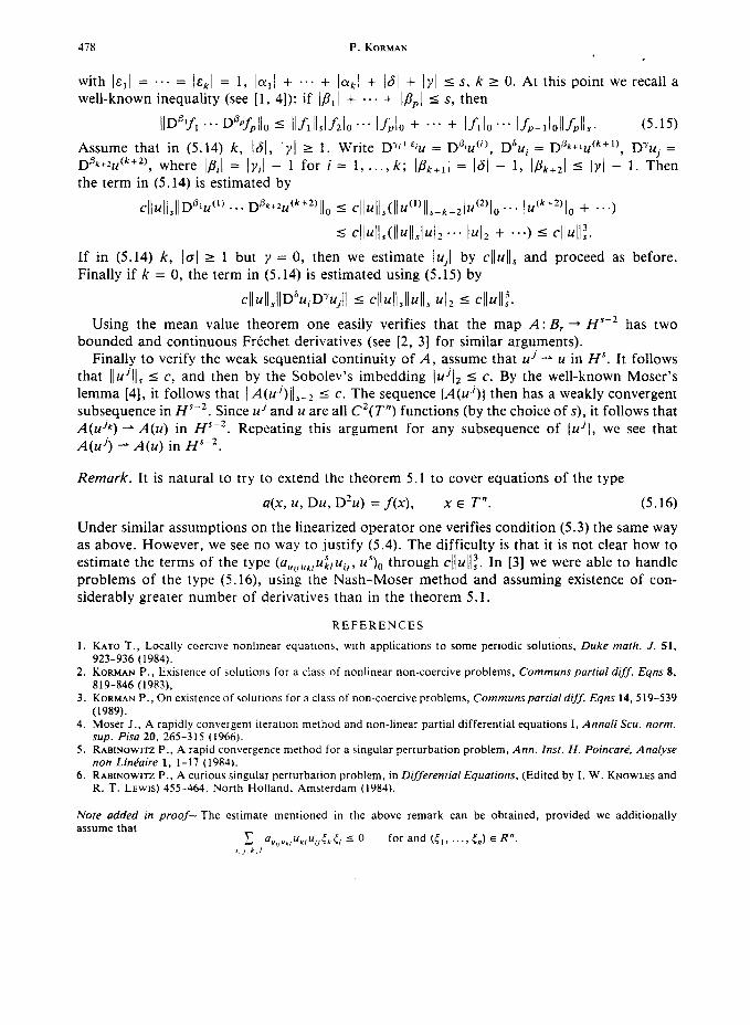
478 P. KORMAN

with 1~~1 = ... = 1~~1 = 1, Ia,/ + ... + Ialrl + 161 + IyI s S, k 2 0. At this point we recall a well-known inequality (see [l, 41): if I/?, I + a.. -C l/1,1 5 s, then

llD!f* ... Da?&!, 5 Ilfiilrlfilo ... l&l, + ... + Ifi e.0 IfP-&llfPlls. (5.15)

Assume that in (5.14) k, (61, 1~1 2 1. Write D’l+% = D%(‘), D”u; = DSk+l~(k+l), DYUj = D17k+%(k+2), where Ipi1 = Iyil - 1 for i = 1, . . ., k; I&+J = 14 - 1, IPk+21 5 Id - 1. Then the term in (5.14) is estimated by

+~I,IIDPI#) . . . D~*+~u(‘+*)II ” S CIIUlls(llU(L)Ils_k_2/U(2)10 0.. lU(k+2)10 + . ..)

5 cII4I,(Il4I,I42 ... I42 + .**I 5 Mll.

If in (5.14) k, lri 1 1 but y = 0, then we estimate lujl by cIJuJI, and proceed as before. Finally if k = 0, the term in (5.14) is estimated using (5.15) by

cIIuIIsIID6UiDYUjII 5 cII~II,II~II,I~I~ 5 dbli2. Using the mean value theorem one easily verifies that the map A: B, + H”-* has two

bounded and continuous Frkchet derivatives (see [2, 31 for similar arguments). Finally to verify the weak sequential continuity of A, assume that uj - u in H”. It follows

that lluiIIS I c, and then by the Sobolev’s imbedding (&I2 5 c. By the well-known Moser’s lemma [4], it follows that IIA(uj)ilS_2 5 c. The sequence (A( then has a weakly convergent subsequence in Hs-*. Since uj and u are all C’(7’“) functions (by the choice of s), it follows that A(&‘) - .4(u) in Hs-*. Repeating this argument for any subsequence of (uj], we see that A(&) - A(u) in Hs-*.

Remark. It is natural to try to extend the theorem 5.1 to cover equations of the type

a(x, u, Du, D*u) = f(x), x E T”. (5.16)

Under similar assumptions on the linearized operator one verifies condition (5.3) the same way as above. However, we see no way to justify (5.4). The difficulty is that it is not clear how to estimate the terms of the type (au,,ur, kl ,J, us u.. u’)~ through cll~ll,‘. In [3] we were able to handle problems of the type (5.16), using the Nash-Moser method and assuming existence of con- siderably greater number of derivatives than in the theorem 5.1.

REFERENCES

1. KATO T., Locally coercive nonlinear equations, with applications to some periodic solutions, Duke math. J. 51, 923-936 (1984).

2. KORMAN P., Existence of solutions for a class of nonlinear non-coercive problems, Communs partial diff. Eqns 8, 819-846 (1983).

3. KORMAN P., On existence of solutions for a class of non-coercive problems, Communsparrialdiff. Eqns 14,519-539 (1989).

4. Moser J., A rapidly convergent iteration method and non-linear partial differential equations I, Anna/i Scu. norm. sup. Piss 20, 265-315 (1966).

5. RABINOWITZ P., A rapid convergence method for a singular perturbation problem, Ann. Inst. H. PoincurP, Analyse non Lin&ire 1, 1-17 (1984).

6. RA~INOWITZ P., A curious singular perturbation problem, in Differenrial Equofions, (Edited by I. W. KNOWLES and R. T. L~wrs) 455-464. North Holland, Amsterdam (1984).

Nore added in proof-The estimate mentioned in the above remark can be obtained, provided we additionally assume that

I: au,,ux,ukIu,,~k~i 5 0 for and (c,, . ., 5,) E R”.