computational methods for structural bioinforamtics...
TRANSCRIPT
Computational Methods for Structural
Bioinforamtics
and Computational Biology (1)
(Sequence comparison)
Jie Liang 梁 杰
Molecular and Systems Computational Bioengineering Lab (MoSCoBL)Department of Bioengineering
University of Illinois at Chicago上海交通大学系统医学研究院
上海生物信息技术研究中心
E-mail: [email protected]/~jliang
Dragon Star Short CourseSuzhou University, June 15 – June 19, 2009

June 15 – June 19
Working language in Chinese; slides in English
Discussions are encouraged throughout the lectures
Lectures will focus on fundamental, while students are welcome to challenge the instructor with any questions related to the subject
Additional discussion session
Course Organization

Reference Books
“"Introduction to Computational Molecular Biology" by Carlos Setubaland Joao Meidanis, 1997, PWS Publishing, ISBN 0534952623 “Computational Molecular Biology” by Peter Clote and Rolf Backofen, John Wiley, 2000, ISBN-471-87251-2. . “Geometry and topology for mesh generation” by Herbert Edelsbrunner”, Cambridge University Press, 2001, ISBN 0-521-79309-2“Monte Carlo Strategies in Scientific Computing” by Jun S. Liu (Springer Series in Statistics), 2009 (Paperback), ISBN-10: 0387763694
"Biological Sequence Analysis: Probabilistic Models of Proteins and Nucleic Acids" by Richard Durbin, Sean R. Eddy, Anders Krogh, and Graeme Mitchison, Cambridge University Press, 1999, ISBN 0521629713“Monte Carlo Statistical Methods” by Christian P. Robert and George Casella, Springer, 2005, ISBN-10: 0387212396
A Brief Survey
Computer science background?
Biology background?
Mathematics/Statistical background?
None of above?
Have you taken another bioinformatics course?

Prerequisites
Basic knowledge of computer science
Assume no prior knowledge in biology above high school
Strong motivation in learning bioinformatics and computational biology
Today’s Lecture
Scope of bioinformatics and the courseBasic concepts in molecular biology: DNA, RNA, protein, Dynamic programming and pairwise sequence analysisStatistical models for evaluating aligned sequencesOptimal multiple sequence alignmentHeuristic multiple sequence alignment
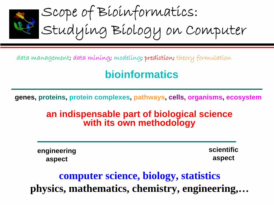
Scope of Bioinformatics: Studying Biology on Computer
data management; data mining; modeling; prediction; theory formulation
engineering aspect
scientific aspect
bioinformatics
an indispensable part of biological sciencewith its own methodology
genes, proteins, protein complexes, pathways, cells, organisms, ecosystem
computer science, biology, statisticsphysics, mathematics, chemistry, engineering,…

Why Bioinformatics? (I)
More than 80 US universities offer graduate degrees in bioinformatics
At cross-section of two most exciting fields: computer science and biology
Exponential growths in computing technologies (hardware, Internet) pave the way for bioinformatics development

Why Bioinformatics? (II)
Analytical technology
High-throughput data
Biological knowledge
Medicine & bioengineering
What Can Computing Do for Biology?
1.
Data interpretation in analytical technologies
2.
Data management and computational infrastructure
3.
Discovery from data mining
4.
Physical models through computing, prediction, and design
5.
Theoretical / in silico biology
Almost every area of computer science can be applied to biologyMany computer scientists study biological problems
1. Data Interpretation in Analytical Technologies (I)
Analytical technologies are the driving force of new (large-scale) biology:
DNA sequencing (genomics)
X-ray / NMR structure determination (structural genomics)
Protein identification using mass spectrometry (proteomics)
Microarray chips (functional genomics)

i+4 i+3i+2
ii-1
i+1
CRH
N NC
CC
RO
H H
H
HNCC
O
H HNCC
O
H H
CRH
NMR spectra
peak assignment
structuralrestraint
extraction
protein structure
structure calculation
1. Data Interpretation in Analytical Technologies (II)
NMR protein structure determination

1. Data Interpretation in Analytical Technologies (III)
From image to data (imaging processing)
Large-scale data cannot be handled without computer
Noisy data (optimization with under-constraint / over-constraint)
Computer algorithms/programs can mimic human interpretation process and do it much faster
Automation of experimental data interpretation
2. Data Management and Computational Infrastructure
Track instruments, experiment conditions and results at each step of a complicated biological experiment (LIMS at modern wet labs)
Data storage and retrieval (database)
Data visualization
Data query and analysis pipeline
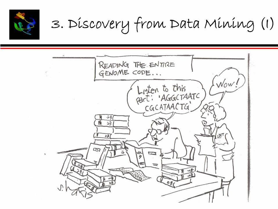
3. Discovery from Data Mining (I)

Pattern/knowledge discovery from datamany biological data are generated by biological processes which are not well understoodinterpretation of such data requires discovery of convoluted relationships hidden in the data
which segment of a DNA sequence represents a gene, a regulatory regionwhich genes are possibly responsible for a particular disease
Complicated dataLarge-scale, high-dimensionNoisy (false positives and false negatives)
3. Discovery from Data Mining (II)

4. Modeling, Prediction and Design (I)
Modeling and prediction of biological objects/processes
modeling of biochemistry
enzyme reaction rates
modeling of biophysics
dynamics of biomolecules
modeling of evolution
prediction of phylogeny and substitution pattern

Prediction of outcomes of biological processescomputing will become an integral part of modern biology throughan iterative process of
From prediction to engineering designProtein structure prediction to protein engineeringDesign genetically modified species
model formulation
computational prediction
experimental validation
4. Modeling, Prediction and Design (II)
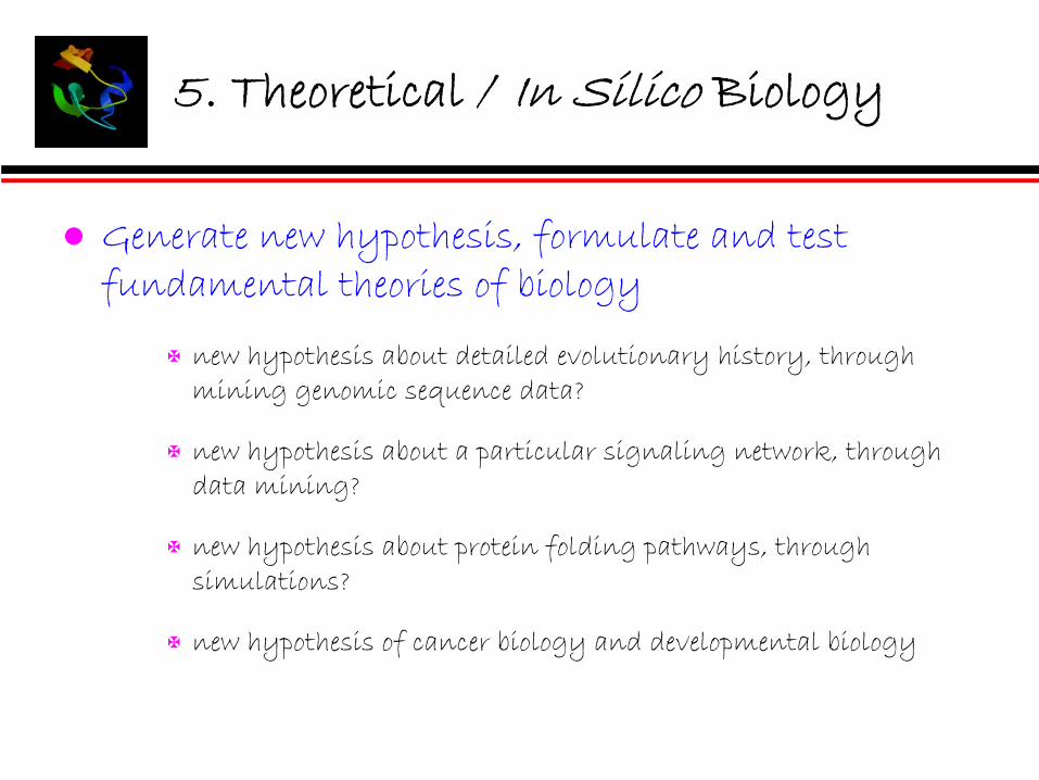
5. Theoretical / In Silico Biology
Generate new hypothesis, formulate and test fundamental theories of biology
new hypothesis about detailed evolutionary history, through mining genomic sequence data?
new hypothesis about a particular signaling network, through data mining?
new hypothesis about protein folding pathways, through simulations?
new hypothesis of cancer biology and developmental biology

Bioinformatics Application to Biological Systems
plants (Arabidopsis)
bacteria(Synechococcus)
viruses (SARS)
yeast (Saccharomyces cerevisia)
neural systems(neurons)

Can Biology Help Computing?
Computational techniques inspired by biology:
Neural network (artificial intelligence)
Genetic algorithm, automata
A new driver of computer science:New algorithms
New driver for theory development
Better hardware (clusters and supercomputers)
Develop new theoretical framework:DNA computing
Network communication,
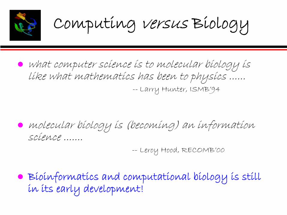
Computing versus Biology
what computer science is to molecular biology is like what mathematics has been to physics ......
-- Larry Hunter, ISMB’94
molecular biology is (becoming) an information science .......
-- Leroy Hood, RECOMB’00
Bioinformatics and computational biology is still in its early development!
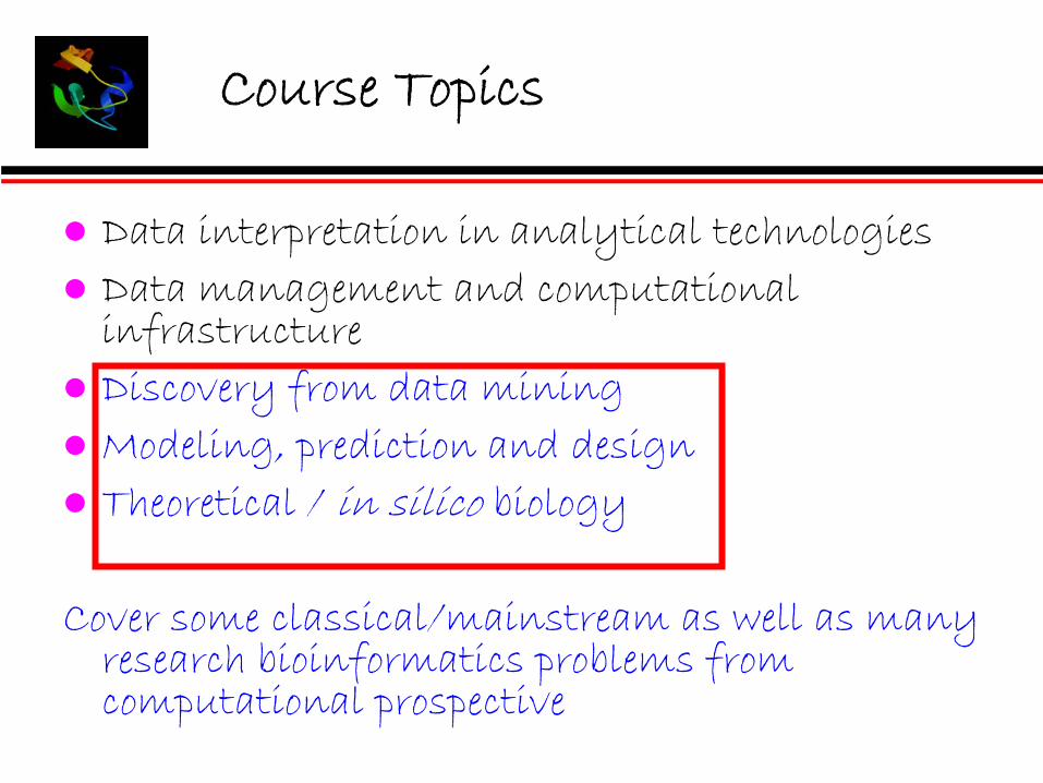
Course Topics
Data interpretation in analytical technologiesData management and computational infrastructureDiscovery from data miningModeling, prediction and designTheoretical / in silico biology
Cover some classical/mainstream as well as many research bioinformatics problems from computational prospective
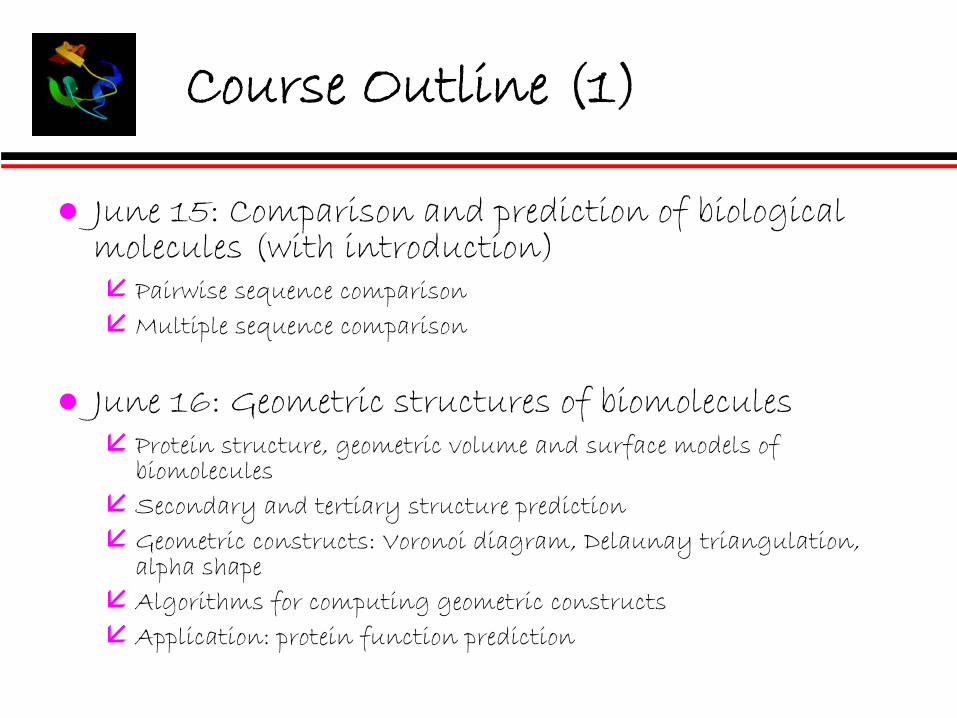
Course Outline (1)
June 15: Comparison and prediction of biological molecules (with introduction)
Pairwise sequence comparisonMultiple sequence comparison
June 16: Geometric structures of biomoleculesProtein structure, geometric volume and surface models of biomoleculesSecondary and tertiary structure predictionGeometric constructs: Voronoi diagram, Delaunay triangulation, alpha shapeAlgorithms for computing geometric constructsApplication: protein function prediction
Course Outline (2)
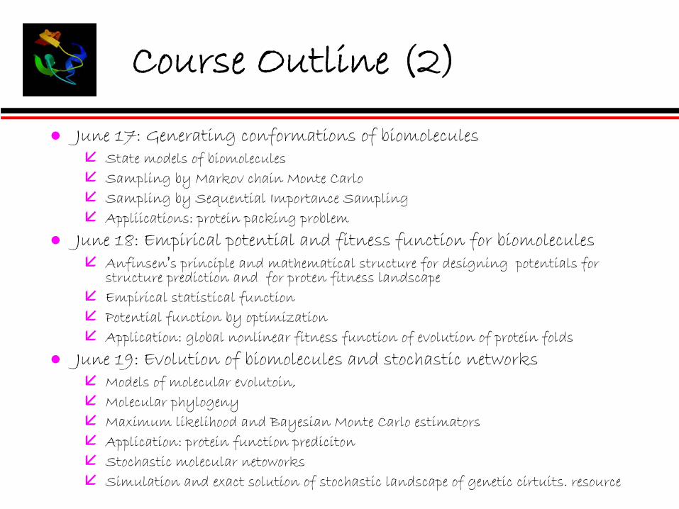
June 17: Generating conformations of biomoleculesState models of biomoleculesSampling by Markov chain Monte CarloSampling by Sequential Importance SamplingAppliications: protein packing problem
June 18: Empirical potential and fitness function for biomoleculesAnfinsen’s principle and mathematical structure for designing potentials for structure prediction and for proten fitness landscapeEmpirical statistical functionPotential function by optimizationApplication: global nonlinear fitness function of evolution of protein folds
June 19: Evolution of biomolecules and stochastic networksModels of molecular evolutoin, Molecular phylogenyMaximum likelihood and Bayesian Monte Carlo estimatorsApplication: protein function predicitonStochastic molecular netoworksSimulation and exact solution of stochastic landscape of genetic cirtuits. resource

What I Will Teach
A general introduction to a few important problems in bioinformatics and computational biology
problems definitions: from biological problem to computable problemsome key aspects of models, theories, algorithms, and computational techniques
A way of thinking: tackling “biological problem” computationally
how to look at a biological problem from a computational point of viewhow to formulate a computational problem to address a biological issuehow to collect statistics from biological datahow to build a computational modelhow to design algorithms for the modelhow to test and evaluate a computational algorithmhow to gain confidence of a prediction result
New Ways of Thinking
Critical thinking
Analytical thinking
Quantitative thinking
Algorithmic thinking
Introduction (1)
Biological sequence comparisonDNA-DNA
RNA-RNA
Protein-protein
Sequence comparison is the most important and fundamental operation in bioinformatics
Key to understand evolution of a gene or an organism
Introduction (2)
Applications in most bioinformatics problems
Sequence assembly
Gene finding
Protein structure prediction
Evolutionary analysis
THE most popular tool: BLAST
Foundation of sequence database search

Today’s Lecture
Scope of bioinformatics and the course
Sequence comparison
Genome
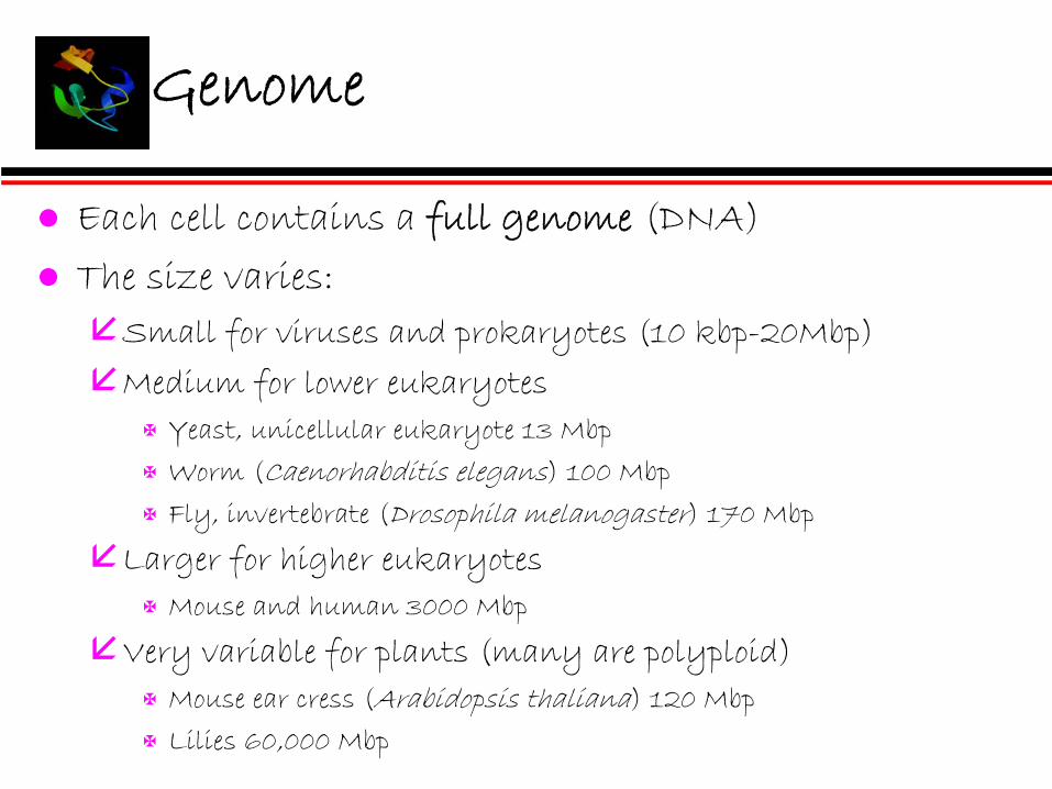
Each cell contains a full genome (DNA)
The size varies:Small for viruses and prokaryotes (10 kbp-20Mbp)
Medium for lower eukaryotesYeast, unicellular eukaryote 13 Mbp
Worm (Caenorhabditis elegans) 100 Mbp
Fly, invertebrate (Drosophila melanogaster) 170 Mbp
Larger for higher eukaryotesMouse and human 3000 Mbp
Very variable for plants (many are polyploid)Mouse ear cress (Arabidopsis thaliana) 120 Mbp
Lilies 60,000 Mbp

Differences in DNA
~2% ~4%
~0.2%
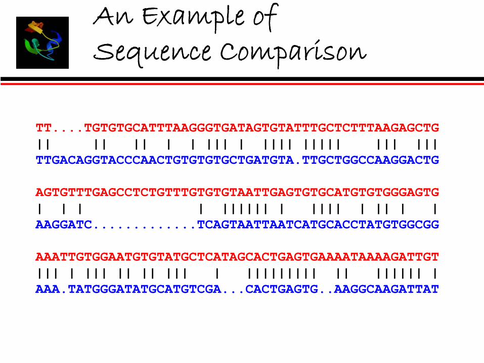
An Example of Sequence Comparison
TT....TGTGTGCATTTAAGGGTGATAGTGTATTTGCTCTTTAAGAGCTG|| || || | | ||| | |||| ||||| ||| |||TTGACAGGTACCCAACTGTGTGTGCTGATGTA.TTGCTGGCCAAGGACTG
AGTGTTTGAGCCTCTGTTTGTGTGTAATTGAGTGTGCATGTGTGGGAGTG| | | | |||||| | |||| | || | |AAGGATC.............TCAGTAATTAATCATGCACCTATGTGGCGG
AAATTGTGGAATGTGTATGCTCATAGCACTGAGTGAAAATAAAAGATTGT||| | ||| || || ||| | ||||||||| || |||||| |AAA.TATGGGATATGCATGTCGA...CACTGAGTG..AAGGCAAGATTAT

Alignement (1)
a correspondence between elements of two sequences with order kept
pairwise alignment: 2 sequences aligned
multiple alignment: alignment of 3 or
FSEYTTHRGHR: ::::: ::FESYTTHRPHR
FESYTTHRGHR:::::::: ::FESYTTHRPHR
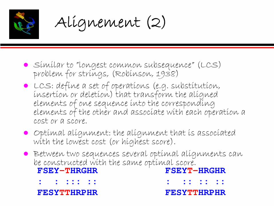
Similar to ”longest common subsequence” (LCS) problem for strings, (Robinson, 1938)LCS: define a set of operations (e.g. substitution, insertion or deletion) that transform the aligned elements of one sequence into the corresponding elements of the other and associate with each operation a cost or a score.Optimal alignment: the alignment that is associated with the lowest cost (or highest score).Between two sequences several optimal alignments can be constructed with the same optimal score.
Alignement (2)
FSEY-THRGHR: : ::: ::FESYTTHRPHR
FSEYT-HRGHR: :: :: ::FESYTTHRPHR

Some Terminology
Alphabet: a finite set of characters from which strings are made. Eg. {A,T,G,C}, twenty amino acid residues.
String: ordered succession of characters or symbols. It is synonymous to sequence.Length of a string s: denoted as |s|, it is the number of characters in it. The character at position i is s(i).
Concatenation: Concatenation of two strings s and t is denoted by st and is given by appending all characters of string t in sequence after those of s. The length of this is |s|+|t|.
If s = GGCTA and t = CAAC, then st = GGCTACAAC.
Prefix: A prefix of s is any substring of s of the form s [ 1...j ] for 0 <= j <= |s|.
Special case: We allow j=0 such that s[1...0] is the empty string, which is also a prefix of s.
t is a prefix of s if and only if there is another string u such that s = tu.
Prefix(s,k) denotes a prefix of s with exactly k characters, with 0<=k<=|s|.
Suffix: A suffix of s is a substring of the form s[i...|s|] for a certain i such that 1<= i<=|s|+1.
We allow i=|s|+1, in which case s[|s|+1...s] denotes the empty string.
A string t is a suffix of s iff there exists u such that s = ut.

Components of Sequence Alignment
FDSK-THRGHR:.: :: :::FESYWTH-GHR
Match (:) Mismatch(substitution)
Insertion Deletion
Indel(1) Scoring function: a measure of similarity between elements (nucleotides, amino acids, gaps);
(2) An algorithm for alignment;
(3) Confidence assessment of alignment result.
Edit Distance (Hamming Distance)
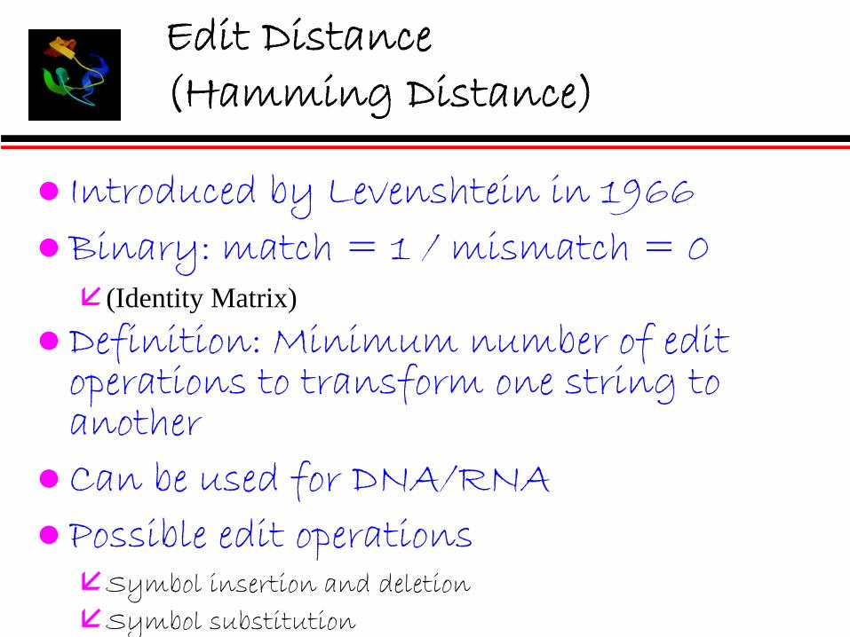
Introduced by Levenshtein in 1966Binary: match = 1 / mismatch = 0
(Identity Matrix)Definition: Minimum number of edit operations to transform one string to anotherCan be used for DNA/RNAPossible edit operations
Symbol insertion and deletionSymbol substitution

amino acid substitution matrices (20X20) account for probability of one amino acid being substituted for another:
frequency of substitution - genetic codetolerance for changes - natural selection
penalize residues pairs with a low probability of mutation in evolution and rewards pairs with a high probability
empirically derived from observed amino acid substitutions that occur between aligned residues in homologous sequences
Scoring Matrix
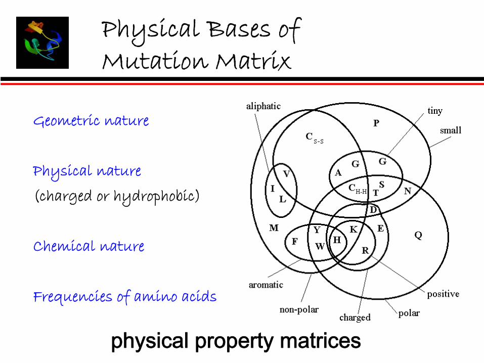
Physical Bases of Mutation Matrix
Geometric nature
Physical nature
(charged or hydrophobic)
Chemical nature
Frequencies of amino acids
physical property matrices
PAM
The first substitution matrices derived by Dayhoff et al. (1978)
PAM (point accepted mutation) distance: Two sequences are defined to have diverged by one PAM unit if they show in average one accepted point mutation (i.e. one amino acid change) per hundred amino acids.
Derived from the pairwise alignment of sequences less than 15% divergent.
BLOSUM
Block substitution matrices (Henikoff & Henikoff1992)
Blocks: highly conserved regions in a set of aligned protein sequences (local multiple alignment)
Number of BLOSUM matrix (e.g. BLOSUM 62) indicates the cutoff of percent identity that defines the clusters - lower cutoffs allow more diverse sequences

A R N D C Q E G H I L K M F P S T W Y V
ARNDCQEGHILKMFPSTWYV
4-1 5-2 0 6-2 -2 1 60 -3 -3 -3 9
-1 1 0 0 -3 5-1 0 0 2 -4 2 50 -2 0 -1 -3 -2 -2 6
-2 0 1 -1 -3 0 0 -2 8 -1 -3 -3 -3 -1 -3 -3 -4 -3 4 -1 -2 -3 -4 -1 -2 -3 -4 -3 2 4 -1 2 0 -1 -3 1 1 -2 -1 -3 -2 5 -1 -1 -2 -3 -1 0 -2 -3 -2 1 2 -1 5 -2 -3 -3 -3 -2 -3 -3 -3 -1 0 0 -3 0 6 -1 -2 -2 -1 -3 -1 -1 -2 -2 -3 -3 -1 -2 -4 7 1 -1 1 0 -1 0 0 0 -1 -2 -2 0 -1 -2 -1 4 0 -1 0 -1 -1 -1 -1 -2 -2 -1 -1 -1 -1 -2 -1 1 5
-3 -3 -4 -4 -2 -2 -3 -2 -2 -3 -2 -3 -1 1 -4 -3 -2 11 -2 -2 -2 -3 -2 -1 -2 -3 2 -1 -1 -2 -1 3 -3 -2 -2 2 70 -3 -3 -3 -1 -2 -2 -3 -3 3 1 -2 1 -1 -2 -2 0 -3 -1 4
BLOSUM 62 Matrix
Close homolog: high cutoffs for BLOSUM (up to BLOSUM 90) or lower PAM values
BLAST default: BLOSUM 62
Remote homolog: lower cutoffs for BLOSUM (down to BLOSUM 10) or high PAM values (PAM 200 or PAM 250)
A best performer in structure prediction:PAM 250
What Matrices to Use
Gap Penalty Functions
Corresponding to insertion/deletion in evolution
Can be derived from alignmentKnown alignments
Performance-based (sequence comparison)

Affine Gap Penalty Function
If we are introducing k spaces together, the penalty should be less than that for k independent spaces.
i.e.
w (k)
≤
k w(1)
or,
w ( k1
+ k2 +… + kn
)
≤
w ( k1
)
+ w (k2
) +… + w ( kn
).
A function which satisfies the above conditions is called a subadditive function.
An affine function is a function of the form,
w ( k ) = h + g k, k ≥
1,
where w (0) = 0 and h, g > 0.
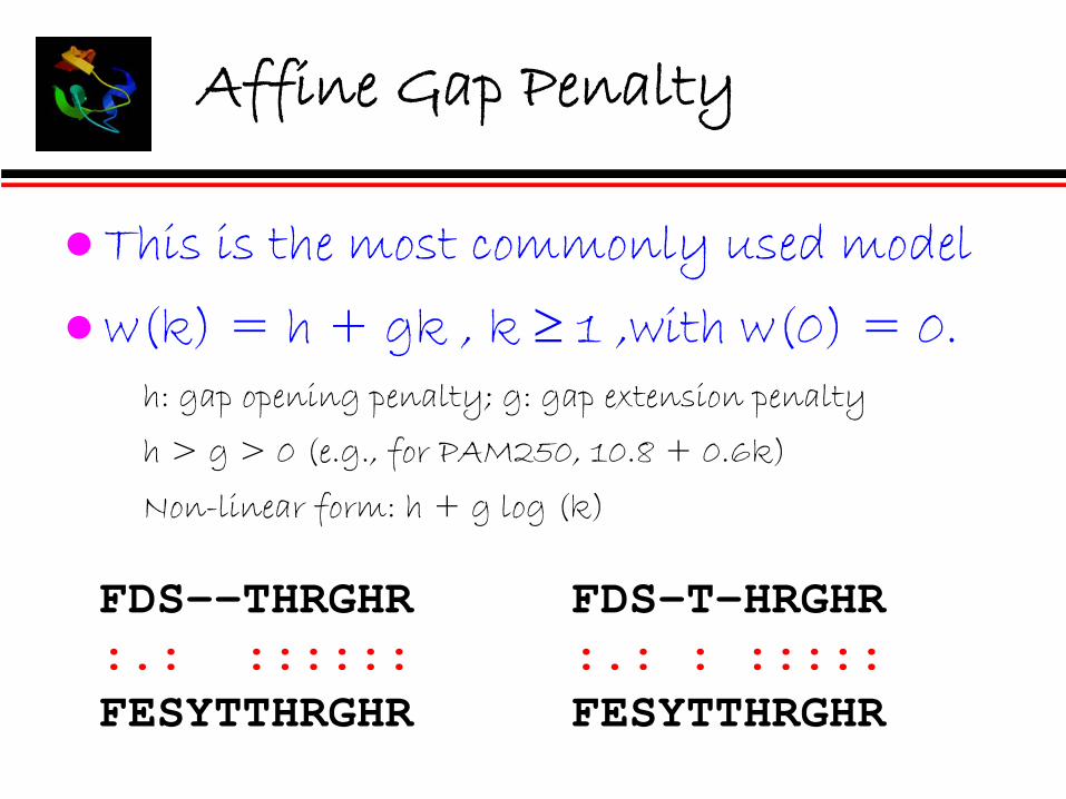
Affine Gap Penalty
This is the most commonly used model
w(k) = h + gk , k ≥ 1 ,with w(0) = 0.h: gap opening penalty; g: gap extension penalty
h > g > 0 (e.g., for PAM250, 10.8 + 0.6k)
Non-linear form: h + g log (k)
FDS-T-HRGHR:.: : :::::FESYTTHRGHR
FDS--THRGHR:.: ::::::FESYTTHRGHR
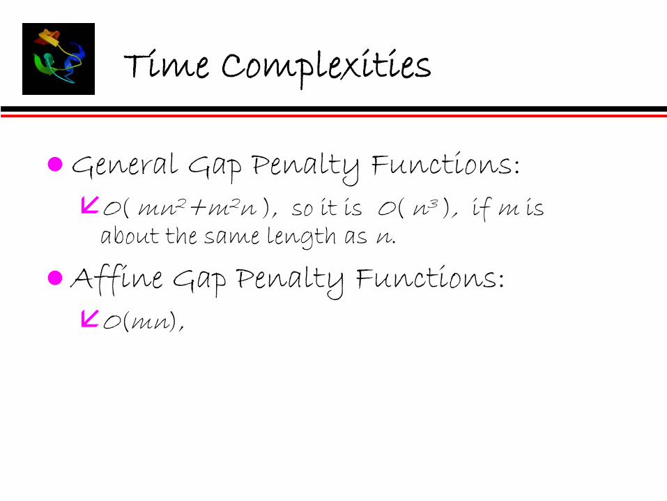
Time Complexities
General Gap Penalty Functions:O( mn2+m2n ), so it is O( n3 ), if m is about the same length as n.
Affine Gap Penalty Functions:O(mn),
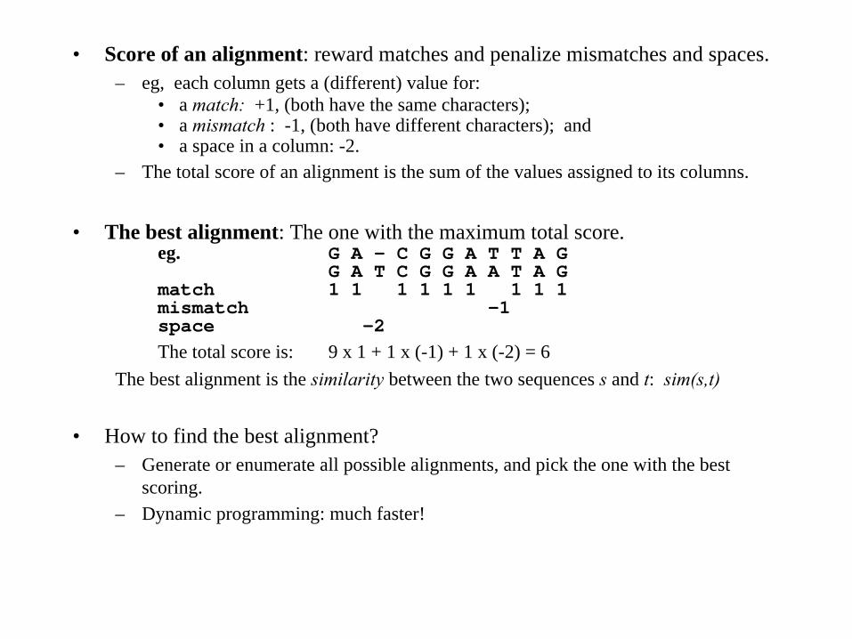
• Score of an alignment: reward matches and penalize mismatches and spaces.– eg, each column gets a (different) value for:
• a match: +1, (both have the same characters); • a mismatch
: -1, (both have different characters); and • a space in a column: -2.
– The total score of an alignment is the sum of the values assigned to its columns.
• The best alignment: The one with the maximum total score.eg. G A - C G G A T T A G
G A T C G G A A T A Gmatch 1 1 1 1 1 1 1 1 1mismatch -1 space -2The total score is: 9 x 1 + 1 x (-1) + 1 x (-2) = 6
The best alignment is the similarity
between the two sequences s
and t: sim(s,t)
• How to find the best alignment?– Generate or enumerate all possible alignments, and pick the one with the best
scoring.– Dynamic programming: much faster!

Dot Matrix and Alignment
A A C G G T A T G CA 1 1 1T 1 1C 1 1G 1 1 1G 1 1 1G 1 1 1T 1 1T 1 1G 1 1 1C 1 1
AACGATCG
-GGTGT
A-TGCTGC
Dot matrix:Score between cross-elements
path:Mapping toan alignment

1.
Assign scores between elements in dot matrix
2.
For each cell in the dot matrix, check all possible pathways back to the beginning of the sequence (allowing insertions and deletions) and give that cell the value of the maximum scoring pathway
3.
Construct an alignment (pathway) back from the last cell in the dot matrix (or the highest scoring) cell to give the highest scoring alignment
Dynamic Programming Steps
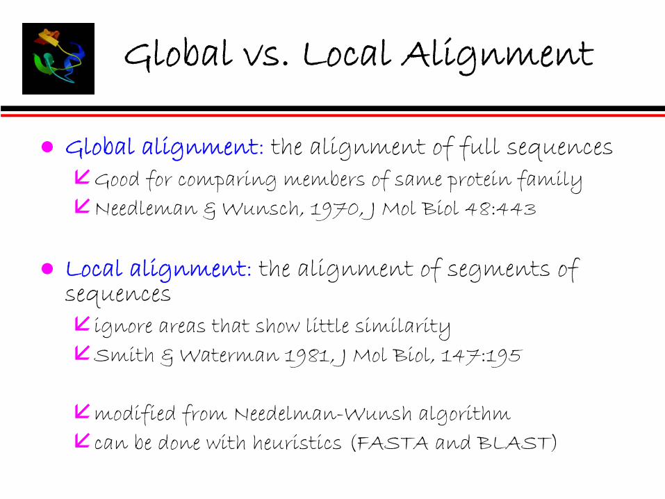
Global alignment: the alignment of full sequences Good for comparing members of same protein familyNeedleman & Wunsch, 1970, J Mol Biol 48:443
Local alignment: the alignment of segments of sequences
ignore areas that show little similaritySmith & Waterman 1981, J Mol Biol, 147:195
modified from Needelman-Wunsh algorithmcan be done with heuristics (FASTA and BLAST)
Global vs. Local Alignment
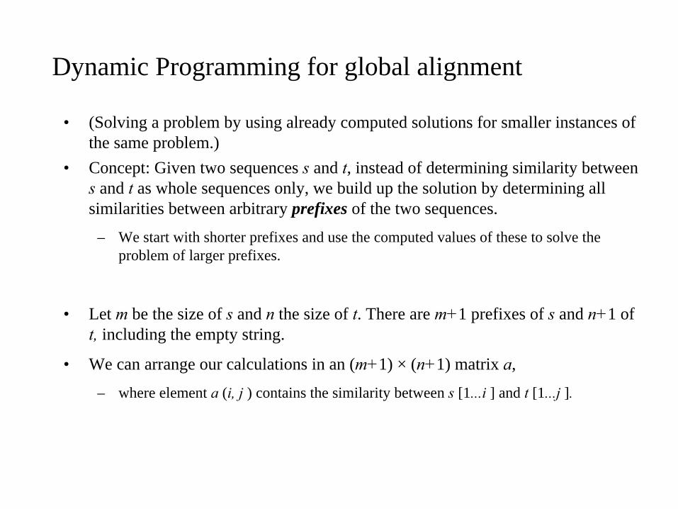
Dynamic Programming for global alignment
• (Solving a problem by using already computed solutions for smaller instances of the same problem.)
• Concept: Given two sequences s
and t, instead of determining similarity between s
and t
as whole sequences only, we build up the solution by determining all
similarities between arbitrary prefixes of the two sequences.
– We start with shorter prefixes and use the computed values of these to solve the problem of larger prefixes.
• Let m
be the size of s
and n
the size of t. There are m+1 prefixes of s
and n+1 of t,
including the empty string.
• We can arrange our calculations in an (m+1) × (n+1) matrix a,
– where element a (i, j ) contains the similarity between s [1...i ] and t [1...j ].

• The matrix a
for s = AAAC and t = AGC– The first row and first column: multiples
of space penalty.– Only one alignment possible if one seq is
empty: add spaces, with score -2k
• Key point: the value for the entry a (i, j) can be obtained by looking at just three previous entries:
– those for ( i -1, j ), ( i-1, j-1 ) and (i, j-1).
• The reason is that there are only three ways to align s [1..i] and t [1..j]
align s[1...i] with t[1...j-1] and match a space with t [ j
]
align s[1...i-1] with t [1...j-1] and match s[i] with t [j].
align s[1...i-1] with t[1...j] and match s[i] with a space.
– These are exhaustive possibilities, since we cannot have two spaces paired.
s(i)
t(j)

For example, the value of a[1, 2] comes from one of the three:a[1, 1] -
2 = -1; a [0, 1] -1 = -3; a [0, 2] -
2 = -6
• sim(s[1...i ], t [1...j ]) = maximum of sim
( s[1...i], t [1...j-1] ) -
2sim
( s[1...i -1], t [1...j-1] )+ p ( i, j )sim
( s[1...i -1], t [1...j] ) - 2
• Since a (i, j) stores sim
(i, j ),
the similarity of s[1...i ] with t[1...j] is:a( s[1...i ], t[1...j] ) = maximum of
a (i, j-1) -
2a (i-1, j-1) + p(i, j)a (i-1, j ) - 2
• Important: the order of the computing needs to make sure that a ( i, j-1 ), a( i-1, j-1 ), and a( i-1, j ) are available when computing a (i, j ).
Here entries are computed row by row, and usually gap g<0
Algorithm to Compute Global Similarity:
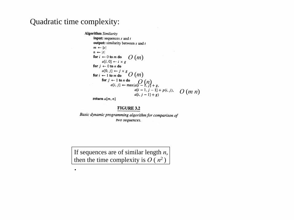
Quadratic time complexity:
O (m)
O (n)O (m n)
If sequences are of similar length n, then the time complexity is O ( n2 ) .
O (m)
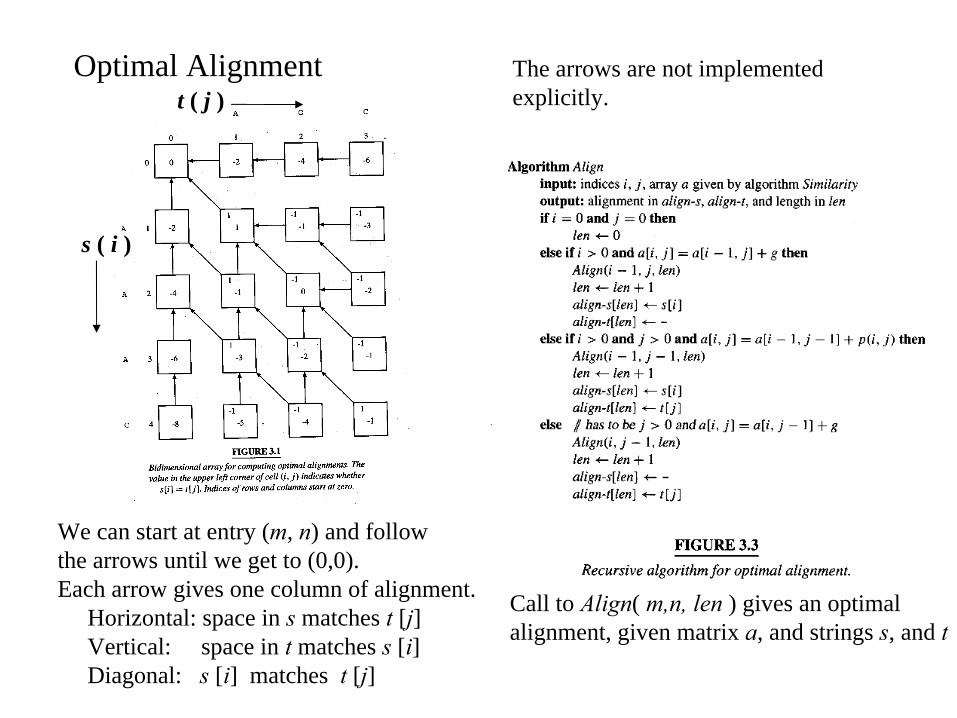
Optimal Alignment
s ( i )
t ( j )
We can start at entry (m, n) and followthe arrows until we get to (0,0).Each arrow gives one column of alignment.
Horizontal: space in s
matches t [j]Vertical: space in t
matches s [i]
Diagonal: s [i] matches t [j]
The arrows are not implementedexplicitly.
Call to Align( m,n, len
) gives an optimalalignment, given matrix a, and strings s, and t

Answers are given in vectors align-sand align-t, holding in 1..len
the aligned characters, symbols or spaces.
Length of the alignment is returned bylen:
max(|s|,|t|) <= len
<= m+n
Time complexity when a matrix is given:
O(len),
the size of the returnedalignment
orO(m+n)
It is possible that several alignmentsmay have the same scores:
+1-1-2 -2+1-1 +1-2-1A A A A A A A A AA G - - A G A - G
The algorithm returns just one, givingpreferences to edges leaving (i, j ) in counterclockwise order.
That is: if there are two or three choices, a column with space in t
is preferred overa column with two symbols, which ispreferred over a column with space over s.
Upmost alignment:This is achieved through the order of if s
egs -ATAT ATAT-t TATA- > -TATA

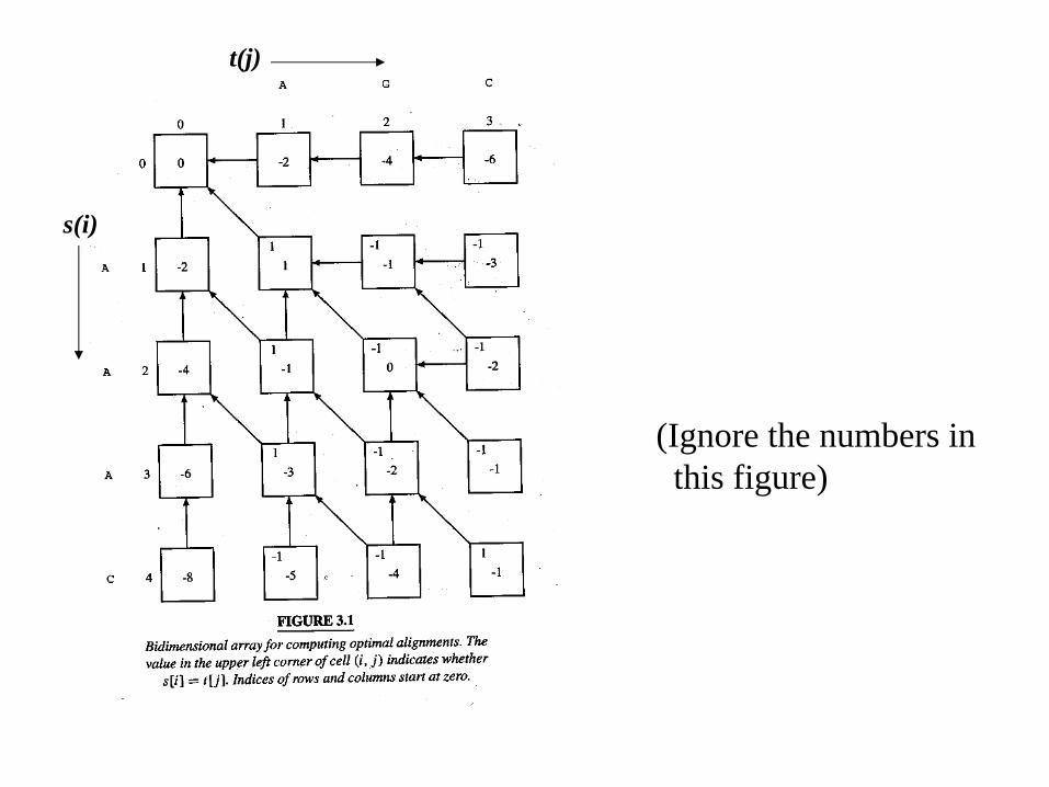
Local Comparison• An alignment between a substring of s
and a substring of t.
• Goal: to find the highest scoring local alignment.
• Same Data structure: an array a[1..m+ 1][1..n+1]– a[i, j] : the highest score of an alignment between a suffix of s[1..i ] and a
suffix of t[1..j]– Because the empty string, which has a score 0, is always a valid suffix of a
sequence, all entries >= 0.– First row and first column: initialize to 0.
• The entrya( s [1...i], t [1...j] ) = maximum of
a (i, j-1 ) - ga (i-1, j-1 ) + p ( i, j )a (i-1, j ) - g
0 ------
an empty alignment
s(i)
t(j)
(Ignore the numbers in this figure)

• Find the maximum entry in the whole array: this is the score of an optimal local alignment.
• Start from any entry with this score value, and trace back until there is no arrow:
– optimal local alignment.
– In general, we are interested in not only the optimal local alignment, but also near optimal alignment.
End Spaces in Alignments: End spaces are before the first character or after the last character.
Consider the following alignment: C A G C A - C T T G G A T T C T C G G size 18 - - - C A G C G T G G - - - - - - - - size 8-2-2-2 -2 -2-2-2-2-2-2-2-2 12x(-2)
-1 -11 1 1 1 1 1 6x 1
There will be many spaces in any alignment because length differences, contributing to a large negative score (-19).
The above alignment is pretty good, if end spaces are ignored: 6 matches, 1 mismatch, 1 space.
• The alignment with the best score is:
CAGCACTTGGATTCTCGGCAGC-----G-T----GG
10x(-2) +8 x 1 = -12
– Although this alignment gives a better score (-12 as compared to -18), it is not interesting because it is not finding similar regions
– We are interested in regions in the longer sequence that are approximately the same as the shorter regions.
• However, if we choose the first alignment and neglect all end spaces, then the score is +3.
Semiglobal Comparison!
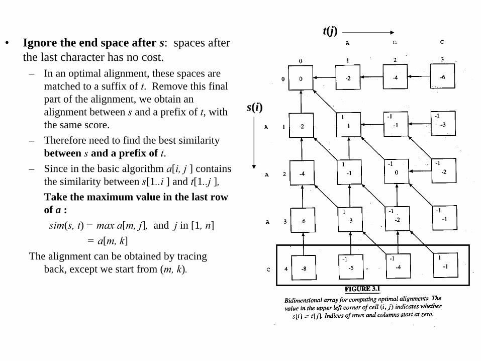
• Ignore the end space after s: spaces after the last character has no cost.
– In an optimal alignment, these spaces are matched to a suffix of t. Remove this final part of the alignment, we obtain an alignment between s
and a prefix of t, with the same score.
– Therefore need to find the best similarity between s
and a prefix of t.– Since in the basic algorithm a[i, j ] contains
the similarity between s[1..i ] and t[1..j ],Take the maximum value in the last row of a :
sim(s, t) = max a[m, j], and j in [1, n]= a[m, k]
The alignment can be obtained by tracing back, except we start from (m, k).
s(i)
t(j)
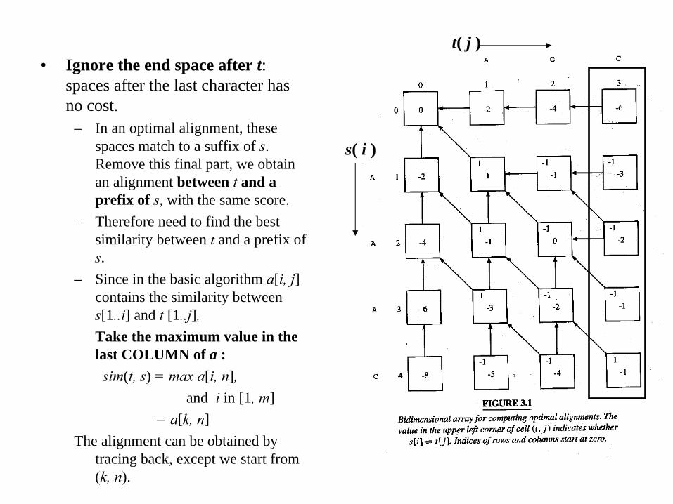
• Ignore the end space after t: spaces after the last character has no cost.
– In an optimal alignment, these spaces match to a suffix of s. Remove this final part, we obtain an alignment between t
and a prefix of s, with the same score.
– Therefore need to find the best similarity between t
and a prefix of s.
– Since in the basic algorithm a[i, j] contains the similarity between s[1..i] and t
[1..j],Take the maximum value in the last COLUMN of a :
sim(t, s) = max a[i, n], and i in [1, m]
= a[k, n]The alignment can be obtained by
tracing back, except we start from (k, n).
s( i )
t( j )

• Ignore the initial space before s: spaces before the first character has no cost.
– This is equivalent to the best alignment between s
and a suffix of t. – a[i, j] needs to contain the highest
similarity between s[1..i] and a suffix of t
[1..j],– Therefore, for s, with |s|=m
and t, with |t|=n, we need to look at a
[m,n].
The matrix can be filled the same way as the basic global algorithm,
But the first row has to be 0: since initial spaces before s
have no costs.
The alignment can be obtained by tracing back from (m, n).
• Ignore the initial spaces before t:Same, except the first column has to be 0.
s(i)
t(j)
First row and col are 0s now.
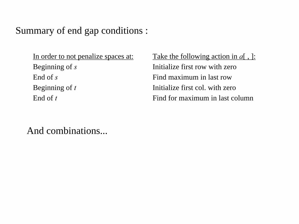
Summary of end gap conditions :
And combinations...
In order to not penalize spaces at: Take the following action in a[ , ]:Beginning of s
Initialize first row with zero
End of s
Find maximum in last rowBeginning of t
Initialize first col. with zero
End of t
Find for maximum in last column

Reading Material
• About dynamic programming in sequence alignment– W.R. Pearson and W.Miller. Methods in Enzymology, 210:575-601, 1992.– T.F.Smith and M.S. Waterman. J. Mol. Biol. 147:195-197, 1981
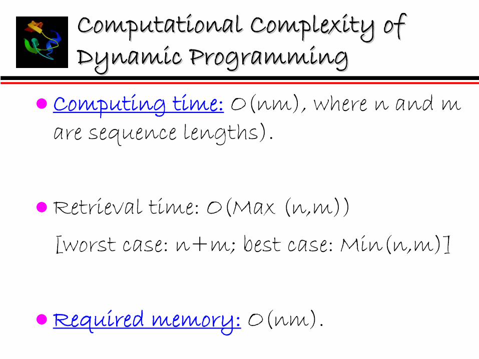
Computational Complexity of Computational Complexity of Dynamic ProgrammingDynamic Programming
Computing time: O(nm), where n and m are sequence lengths).
Retrieval time: O(Max (n,m))
[worst case: n+m; best case: Min(n,m)]
Required memory: O(nm).

Comparing Very similar sequences:
The scores of their optimal alignments are very close to the maximum possible.
For two sequences s and t with the same lengths, The dynamic programming matrix is square.
The main diagonal gives an alignment without spaces.
If that alignment is not optimal, need to add spaces.
We add spaces in pairs, so s and t still have the same lengths:
But now the alignment is off diagonal!
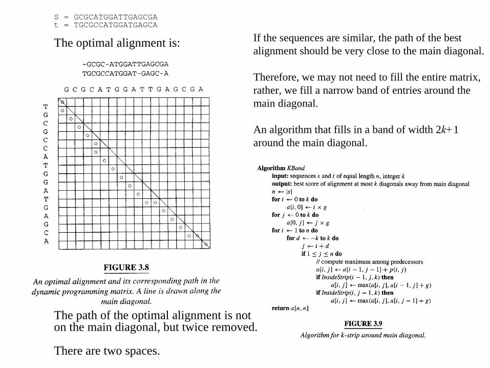
S = GCGCATGGATTGAGCGAt = TGCGCCATGGATGAGCA
The optimal alignment is:
The path of the optimal alignment is noton the main diagonal, but twice removed.
There are two spaces.
If the sequences are similar, the path of the best alignment should be very close to the main diagonal.
Therefore, we may not need to fill the entire matrix,rather, we fill a narrow band of entries around the main diagonal.
An algorithm that fills in a band of width 2k+1 around the main diagonal.

• a
[i,
j] depends on a
[i-1, j
], a
[i-1, j-1],
and a
[i,
j-1].– Do not use any a
[ i-1, j
] and a[ i,
j-1] if they are outside the k-band.– No need to test a[ i-1, j-1
]: it will always be inside the k-band.– For a[i-1, j] and a[ i,
j-1
] , we test because a[i,
j] may be on the border of the band: InsideStrip( i, j, k) = ( - k ≤
i - j ≤
k
) ----------
if this is true: 1
• The entry a[n,
n] contains the highest score of an alignment within the k-band.• The time complexity is O
(kn
),
if k
is modest, this is much better than O
( n2
).
How do we know it is correct if we just look at entries within the k-band?• If there are (k
+1) or more space pairs, the best possible score is when all of the rest
of the sequence match perfectly:match
(n -
k -
1) + 2( k + 1 ) g
– If our k-band computation gives a score better than the above, than there is no need to increase k.
– If not, we need to increase k, and repeat the calculation.– Usually, we double k
and run the calculation again.

Confidence Assessment of Sequence Alignment
Why confidence assessment is needed
True homology or alignment by chance
Expected probability by chance
Statistical models

Why not to use sequence identity as confidence measure

The probability that a variate would assume a value greater than or equal to the observed value strictly by chance P(z>zo)
If the P-value found for an alignment is low (<0.001), the alignment is probably biologically meaningful.
Pre-compute the parameters based on a statistical model
p-value and e-value
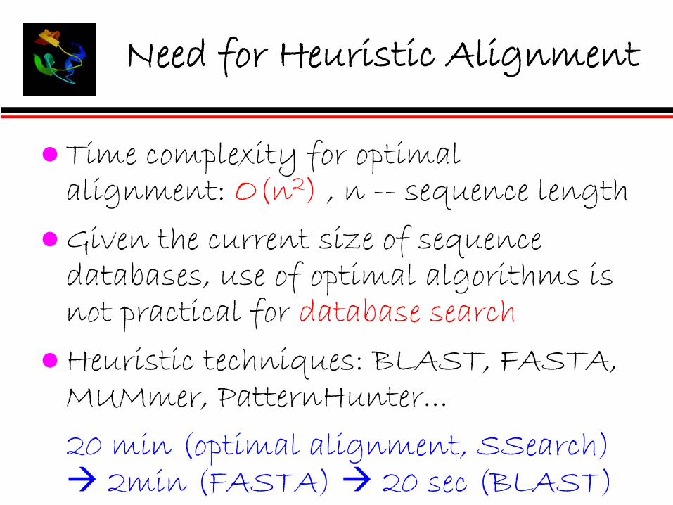
Need for Heuristic Alignment
Time complexity for optimal alignment: O(n2) , n -- sequence length
Given the current size of sequence databases, use of optimal algorithms is not practical for database search
Heuristic techniques: BLAST, FASTA, MUMmer, PatternHunter...
20 min (optimal alignment, SSearch) 2min (FASTA) 20 sec (BLAST)
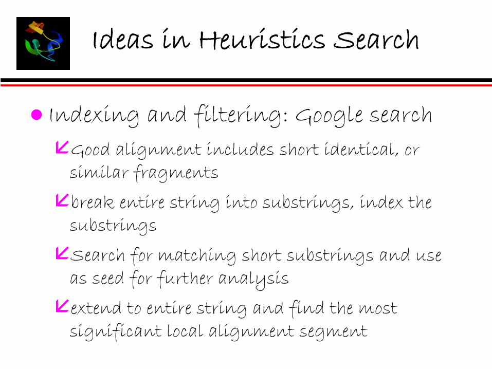
Ideas in Heuristics Search
Indexing and filtering: Google searchGood alignment includes short identical, or similar fragments
break entire string into substrings, index the substrings
Search for matching short substrings and use as seed for further analysis
extend to entire string and find the most significant local alignment segment

FASTA (1)
Lipman & Pearson, 1985, Science 227, 1435-1441
Key ideaIdentify regions of the sequences with the highest density of matches. In this step exact matches of a given length (by default 2 for proteins, 6 for nucleic acids) are determined and regions (fragments of diagonals) with a high number of matches selected.

A-FTFWSYAIGL--PSSSIVSWKSCHVLHKVLRDGHPNVLHDCQRYRSNI| |||||| || || |||| | | |... | : AIPQFWSYAIERPLNSSWIVVWKSCITTHHLMVYGNERFIQYLAS-RNTL
FASTA (2)
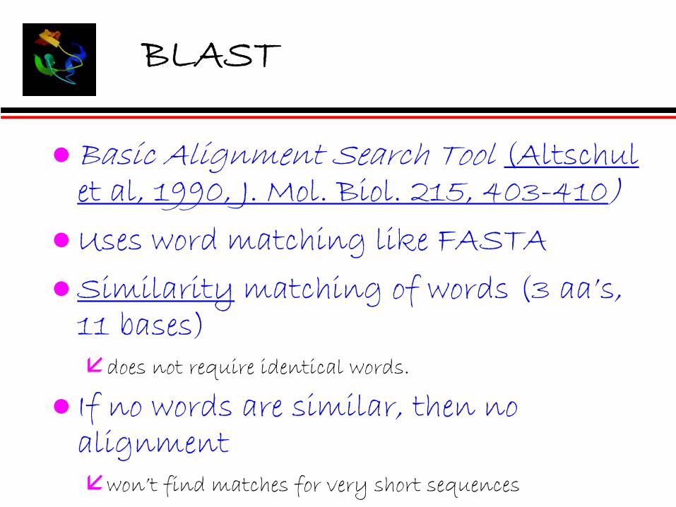
Basic Alignment Search Tool (Altschulet al, 1990, J. Mol. Biol. 215, 403-410)Uses word matching like FASTA
Similarity matching of words (3 aa’s, 11 bases)
does not require identical words.
If no words are similar, then no alignment
won’t find matches for very short sequences
BLAST

Today’s Lecture
Scope of bioinformatics and the course
Pairwise sequence comparison
Multiple sequence comparison
Introduction
The multiple sequence alignment of a set of sequences may be viewed as an evolutionary history of the sequences.
No sequence ordering is required.

An Example of Multiple Alignment
VTISCTGSESNIGAG-NHVKWYQQLPGVTISCTGTESNIGS--ITVNWYQQLPGLRLSCSSSDFIFSS--YAMYWVRQAPGLSLTCTVSETSFDD--YYSTWVRQPPGPEVTCVVVDVSHEDPQVKFNWYVDG--ATLVCLISDFYPGA--VTVAWKADS--AALGCLVKDYFPEP--VTVSWNSG---VSLTCLVKEFYPSD--IAVEWWSNG--
Why Multiple Alignment (1)
Natural extension of Pairwise Sequence Alignment“Pairwise alignment whispers… multiple alignment shouts out loud”
Hubbard et al 1996
Much more sensitive in detecting sequence relationship and patterns

Why Multiple Alignment (2)
Give hints about the function and evolutionary history of a set of sequencesFoundation for phylogenic tree construction and protein family classificationUseful for protein structure prediction…
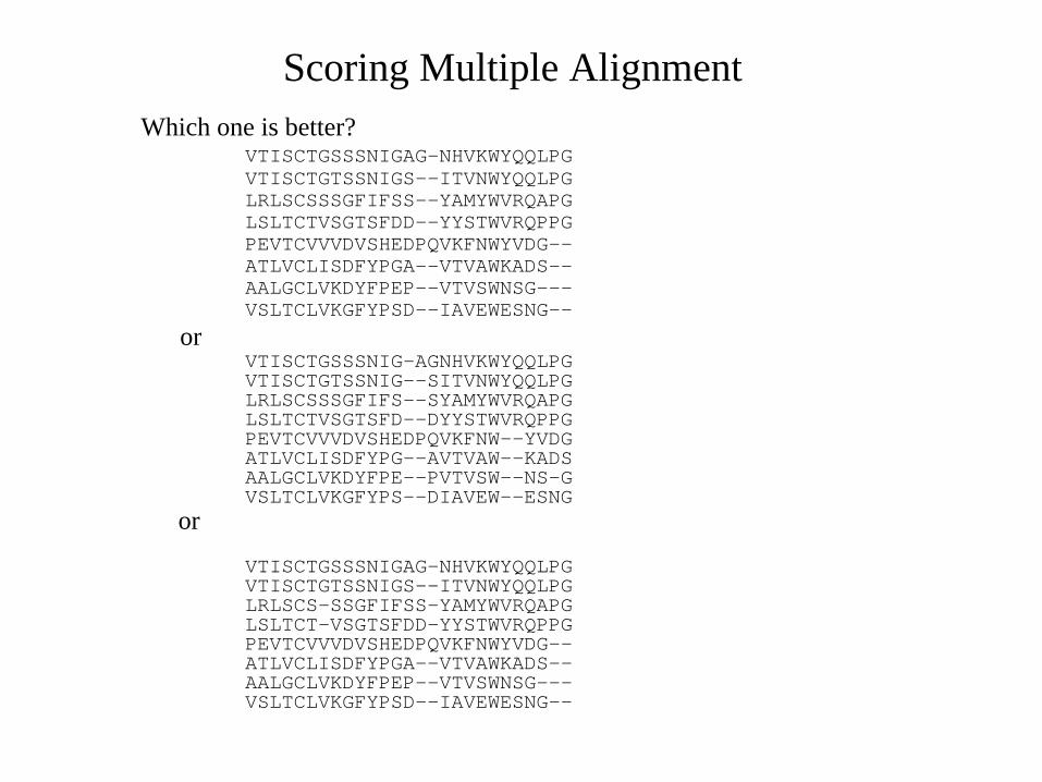
Scoring Multiple AlignmentWhich one is better?
VTISCTGSSSNIGAG-NHVKWYQQLPGVTISCTGTSSNIGS--ITVNWYQQLPGLRLSCSSSGFIFSS--YAMYWVRQAPGLSLTCTVSGTSFDD--YYSTWVRQPPGPEVTCVVVDVSHEDPQVKFNWYVDG--ATLVCLISDFYPGA--VTVAWKADS--AALGCLVKDYFPEP--VTVSWNSG---VSLTCLVKGFYPSD--IAVEWESNG--
orVTISCTGSSSNIG-AGNHVKWYQQLPGVTISCTGTSSNIG--SITVNWYQQLPGLRLSCSSSGFIFS--SYAMYWVRQAPGLSLTCTVSGTSFD--DYYSTWVRQPPGPEVTCVVVDVSHEDPQVKFNW--YVDGATLVCLISDFYPG--AVTVAW--KADSAALGCLVKDYFPE--PVTVSW--NS-GVSLTCLVKGFYPS--DIAVEW--ESNG
or
VTISCTGSSSNIGAG-NHVKWYQQLPGVTISCTGTSSNIGS--ITVNWYQQLPGLRLSCS-SSGFIFSS-YAMYWVRQAPGLSLTCT-VSGTSFDD-YYSTWVRQPPGPEVTCVVVDVSHEDPQVKFNWYVDG--ATLVCLISDFYPGA--VTVAWKADS--AALGCLVKDYFPEP--VTVSWNSG---VSLTCLVKGFYPSD--IAVEWESNG--

Scoring
PQRRZWYQRKZX
YZTUOPTZZ_FO
Total Score = [w(R, U ) + w(R, Δ
) + w(K, U) + w(K, Δ) ] / 4
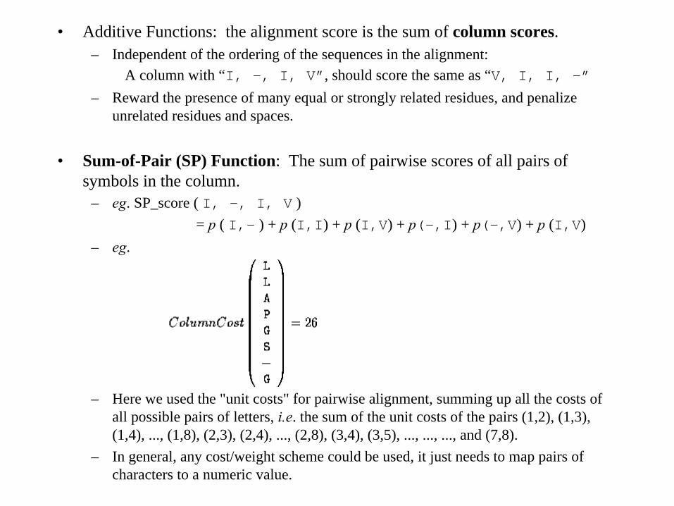
• Additive Functions: the alignment score is the sum of column scores.– Independent of the ordering of the sequences in the alignment:
A column with “I, -, I, V”, should score the same as “V, I, I, -”– Reward the presence of many equal or strongly related residues, and penalize
unrelated residues and spaces.
• Sum-of-Pair (SP) Function: The sum of pairwise scores of all pairs of symbols in the column.
– eg. SP_score ( I, -, I, V )= p
( I,- ) + p
(I,I) + p
(I,V) + p(-,I) + p(-,V) + p
(I,V)– eg.
– Here we used the "unit costs" for pairwise alignment, summing up all the costs of all possible pairs of letters, i.e. the sum of the unit costs of the pairs (1,2), (1,3), (1,4), ..., (1,8), (2,3), (2,4), ..., (2,8), (3,4), (3,5), ..., ..., ..., and (7,8).
– In general, any cost/weight scheme could be used, it just needs to map pairs of characters to a numeric value.
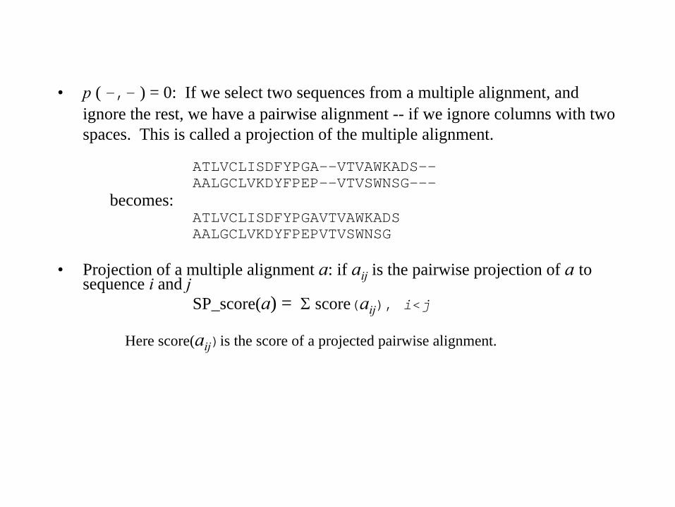
• p
( -,- ) = 0: If we select two sequences from a multiple alignment, and ignore the rest, we have a pairwise alignment -- if we ignore columns with two spaces. This is called a projection of the multiple alignment.
ATLVCLISDFYPGA--VTVAWKADS--AALGCLVKDYFPEP--VTVSWNSG---
becomes:ATLVCLISDFYPGAVTVAWKADSAALGCLVKDYFPEPVTVSWNSG
• Projection of a multiple alignment a: if aij
is the pairwise projection of a to sequence i
and j
SP_score(a) = Σ
score(aij), i<j
Here score(aij)is the score of a projected pairwise alignment.
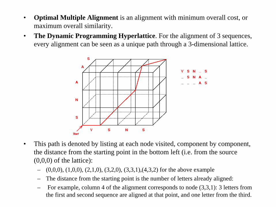
• Optimal Multiple Alignment is an alignment with minimum overall cost, or maximum overall similarity.
• The Dynamic Programming Hyperlattice. For the alignment of 3 sequences, every alignment can be seen as a unique path through a 3-dimensional lattice.
• This path is denoted by listing at each node visited, component by component, the distance from the starting point in the bottom left (i.e. from the source (0,0,0) of the lattice):
– (0,0,0), (1,0,0), (2,1,0), (3,2,0), (3,3,1),(4,3,2) for the above example– The distance from the starting point is the number of letters already aligned:– For example, column 4 of the alignment corresponds to node (3,3,1): 3 letters from
the first and second sequence are aligned at that point, and one letter from the third.

• Imagine light sources on the top, front, and right-hand side of the lattice, "shadows" of the alignment will be projected to the opposing faces (walls).
– Assume that the light sources are farther away from the lattice, and the shadows are projected without distortion.
• In Fig. a, only the light source on the right is "on", projecting the path onto the face on the left.
• In Fig. b, all light sources are "on".
a b
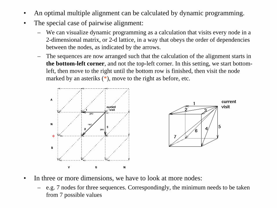
• An optimal multiple alignment can be calculated by dynamic programming.• The special case of pairwise alignment:
– We can visualize dynamic programming as a calculation that visits every node in a 2-dimensional matrix, or 2-d lattice, in a way that obeys the order of dependencies between the nodes, as indicated by the arrows.
– The sequences are now arranged such that the calculation of the alignment starts in the bottom-left corner, and not the top-left corner. In this setting, we start bottom- left, then move to the right until the bottom row is finished, then visit the node marked by an asteriks (*), move to the right as before, etc.
• In three or more dimensions, we have to look at more nodes:– e.g. 7 nodes for three sequences. Correspondingly, the minimum needs to be taken
from 7 possible values

Computational Complexity of Multiple Alignment by Standard Dynamic Programming
• Each node in the k-dimensional hyperlattice is visited once, and therefore the running time must be proportional to the number of nodes in the lattice.
– This number is the product of the lengths of the sequences.– eg. the 3-dimensional lattice as visualized.
• How many steps does the algorithm ``rest'' at each node ?– Dynamic programming organizes the visiting of nodes in such a way that we just
need to ``look back'' one single step, at the nodes that we've visited before, to look up the values we need for calculating the minimum.
– The time we spend for retrieving the minima and calculating the sum does not depend on the length of the sequences.
– However, it depends on the number of sequences. We've had 3 values for 2 sequences, 7 values for 3 sequences, 15 values for 4 sequences. This goes up exponentially: 2k-1
• The running time is expontential: O(2k
Π
|si
|), i = 1.. K– If the proportionality factor is 1 nanosecond, then for 6 sequences of length 100,
we'll have a running time of 26 x 1006 x10-9, that's roughly 64,000 seconds (17 hours). Add two more sequences, then we will have to wait 2.6 x109 = 82 years!
• The memory space requirement is even worse. To trace back the alignment, we need to store the whole lattice, a data structure the size of a multidimensional skyscraper.
– In fact, space is the No.1 problem here, bogging down multiple alignment methods that try to achieve optimality.
– Furthermore, incorporating a realistic gap model, we will further increase our demands on space and running time
As we proceed …
Warning:Muddy Road
Ahead!!!

Progressive Alignment
Devised by Feng and Doolittle in 1987.
A heuristic method, not guaranteed to find the ‘optimal’ alignment.
Multiple alignment is achieved by successive application of pairwisemethods.

Basic Algorithm
Compare all sequences pairwise.
Perform cluster analysis on the pairwisedata to generate a hierarchy for alignment (guide tree).
Build alignment step by step according to the guide tree. Build the multiple alignment by first aligning the most similar pair of sequences, then add another sequence or another pairwise alignments.
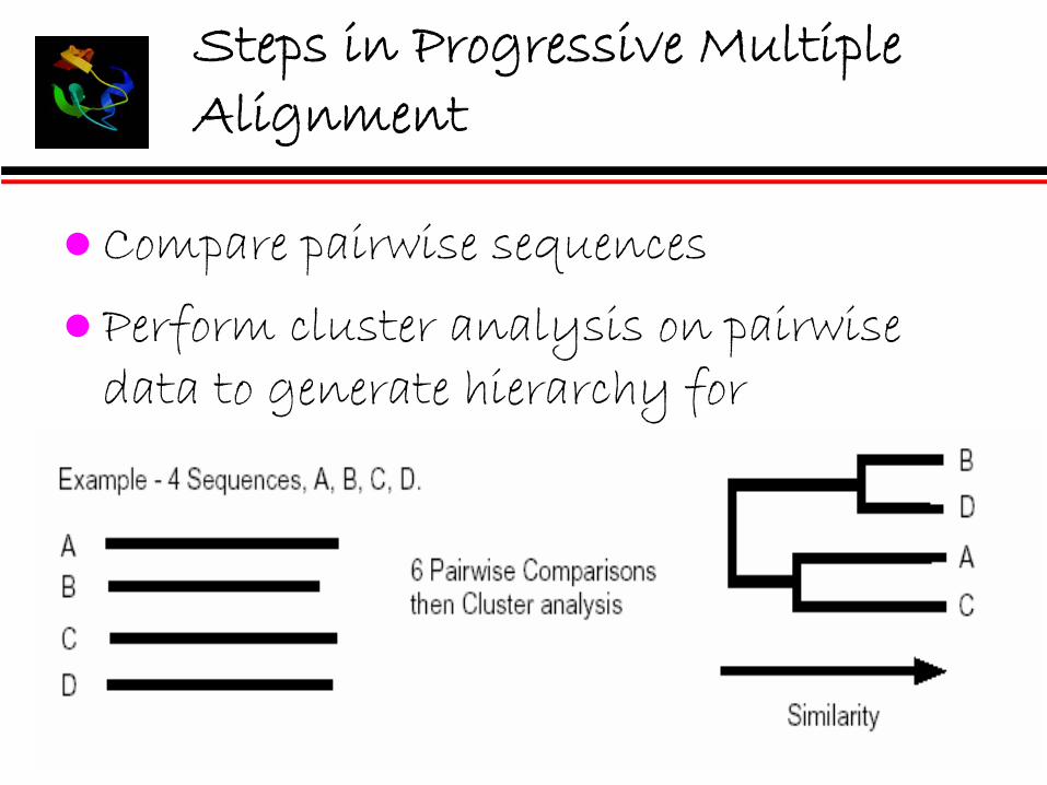
Steps in Progressive Multiple Alignment
Compare pairwise sequences
Perform cluster analysis on pairwisedata to generate hierarchy for alignment
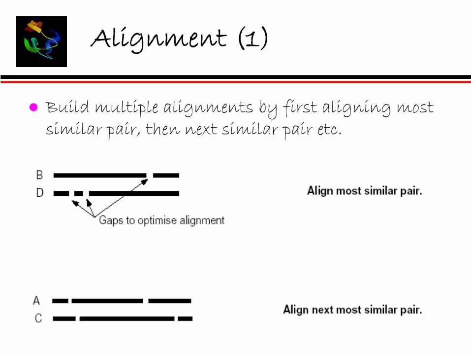
Alignment (1)
Build multiple alignments by first aligning most similar pair, then next similar pair etc.
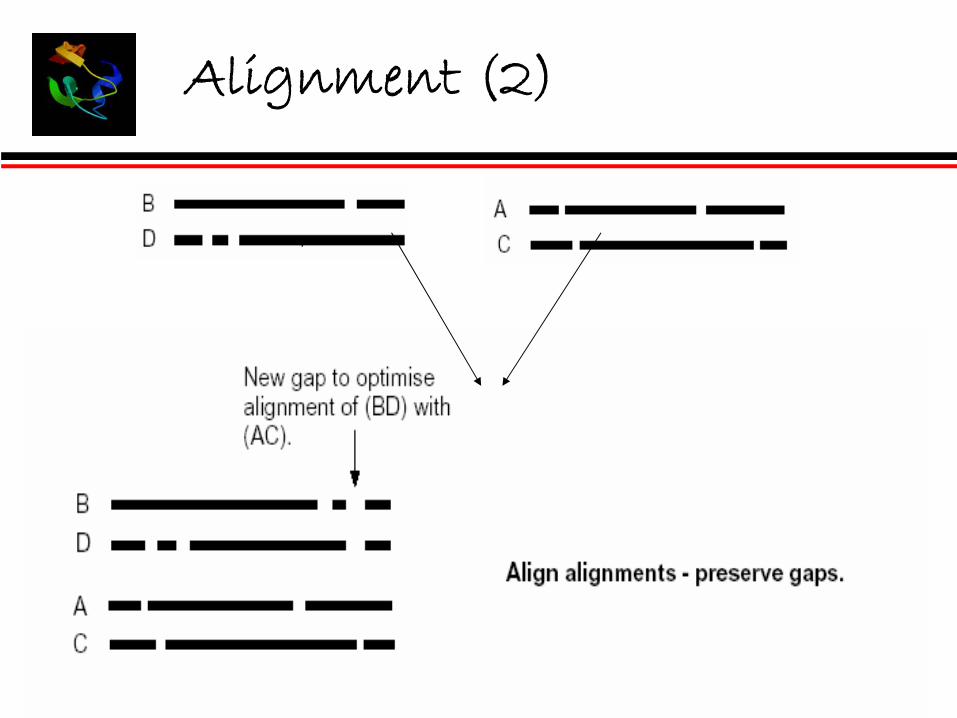
Alignment (2)

Most successful implementation of progressive alignment (Des Higgins)
CLUSTAL - gives equal weight to all sequences
CLUSTALW - has the ability to give different weights to the sequences
CLUSTALX - provides a GUI to CLUSTAL
http://searchlauncher.bcm.tmc.edu/multi-align/multi-align.html
CLUSTAL

Profile-Based Approach
Seq1->
Seq3->Seq4->
Seq2->
Information about the degree of conservation of sequence positions is included
Position-specific Score Matrix (PSSM)
For protein of length L, scoring matrix is L x 20, PSSM(i,j) --“Profile”: specific scores for each of the 20 amino acids at each position in a sequence.For highly conserved residues at a particular position, a high positive score is assigned, and others are assigned high negatives.For a weakly conserved position, a value close to zero is assigned to all the amino acid types.
Building a Profile
First, get multiple sequence alignments using substitution matrix, Sjk.Second, count the number of occurrences of amino acid k at position i, Cik.(1) Average-score method:
Wij
= Σk
Cik
Sjk
/ N.(2) log-odds-ratio formula:
Wij
= log(qij
/pj
).qij
= Cij
/ N.pj
: background probability of residue j.
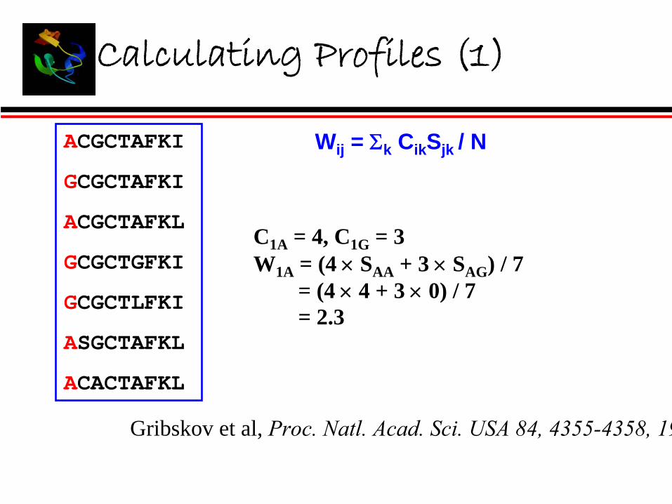
Calculating Profiles (1)
Gribskov et al, Proc. Natl. Acad. Sci. USA 84, 4355-4358, 19
ACGCTAFKI
GCGCTAFKI
ACGCTAFKL
GCGCTGFKI
GCGCTLFKI
ASGCTAFKL
ACACTAFKL
C1A = 4, C1G = 3W1A = (4 ×
SAA + 3 ×
SAG ) / 7
= (4 ×
4 + 3 ×
0) / 7= 2.3
Wij = Σk Cik Sjk / N

Calculating profile (2)
Wij
= log(qij
/pj
).
qij
= Cij
/ N.
pj
: background probability of residue j.
For small N, formula qij = Cij / N is not good A large set of too closely related sequences
carries little more information than a single member.
Absence of Leu does not mean no Leu at this position when Ile is abundant!
Pseudocount frequency, gij
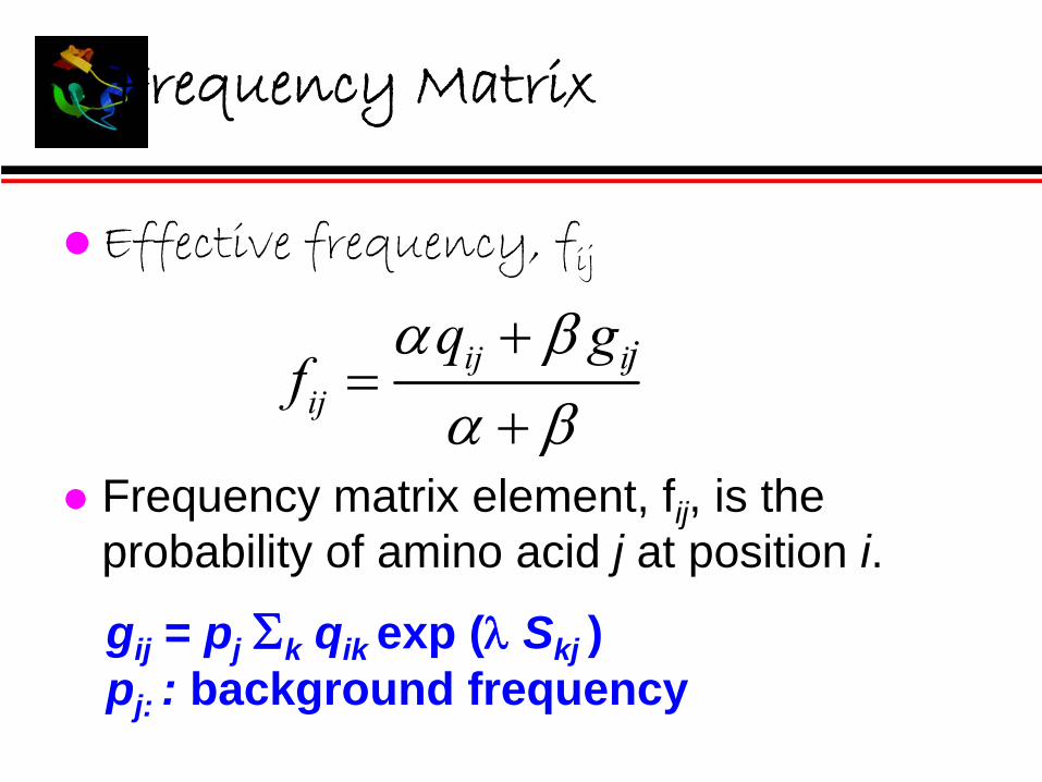
Frequency Matrix
Effective frequency, fij
ij iij
q gf
α βα β+
=+
Frequency matrix element, fij, is the probability of amino acid j at position i.
j
gij = pj Σk qik exp (λ
Skj )pj: : background frequency
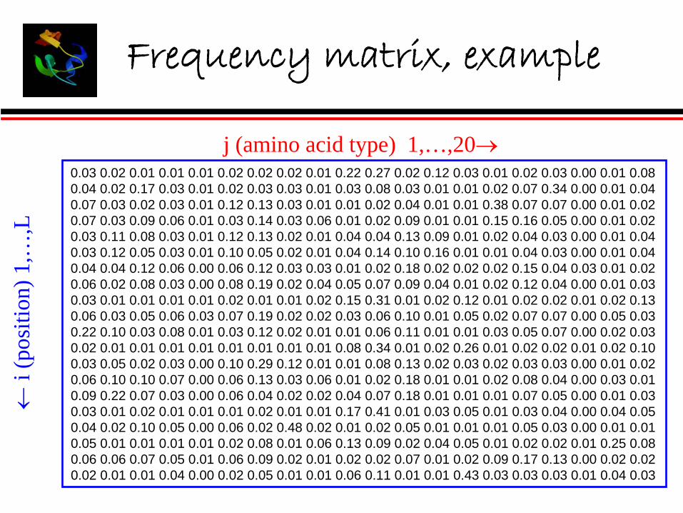
Frequency matrix, example
0.03 0.02 0.01 0.01 0.01 0.02 0.02 0.02 0.01 0.22 0.27 0.02 0.12 0.03 0.01 0.02 0.03 0.00 0.01 0.08 0.04 0.02 0.17 0.03 0.01 0.02 0.03 0.03 0.01 0.03 0.08 0.03 0.01 0.01 0.02 0.07 0.34 0.00 0.01 0.04 0.07 0.03 0.02 0.03 0.01 0.12 0.13 0.03 0.01 0.01 0.02 0.04 0.01 0.01 0.38 0.07 0.07 0.00 0.01 0.02 0.07 0.03 0.09 0.06 0.01 0.03 0.14 0.03 0.06 0.01 0.02 0.09 0.01 0.01 0.15 0.16 0.05 0.00 0.01 0.02 0.03 0.11 0.08 0.03 0.01 0.12 0.13 0.02 0.01 0.04 0.04 0.13 0.09 0.01 0.02 0.04 0.03 0.00 0.01 0.04 0.03 0.12 0.05 0.03 0.01 0.10 0.05 0.02 0.01 0.04 0.14 0.10 0.16 0.01 0.01 0.04 0.03 0.00 0.01 0.04 0.04 0.04 0.12 0.06 0.00 0.06 0.12 0.03 0.03 0.01 0.02 0.18 0.02 0.02 0.02 0.15 0.04 0.03 0.01 0.02 0.06 0.02 0.08 0.03 0.00 0.08 0.19 0.02 0.04 0.05 0.07 0.09 0.04 0.01 0.02 0.12 0.04 0.00 0.01 0.03 0.03 0.01 0.01 0.01 0.01 0.02 0.01 0.01 0.02 0.15 0.31 0.01 0.02 0.12 0.01 0.02 0.02 0.01 0.02 0.13 0.06 0.03 0.05 0.06 0.03 0.07 0.19 0.02 0.02 0.03 0.06 0.10 0.01 0.05 0.02 0.07 0.07 0.00 0.05 0.03 0.22 0.10 0.03 0.08 0.01 0.03 0.12 0.02 0.01 0.01 0.06 0.11 0.01 0.01 0.03 0.05 0.07 0.00 0.02 0.03 0.02 0.01 0.01 0.01 0.01 0.01 0.01 0.01 0.01 0.08 0.34 0.01 0.02 0.26 0.01 0.02 0.02 0.01 0.02 0.10 0.03 0.05 0.02 0.03 0.00 0.10 0.29 0.12 0.01 0.01 0.08 0.13 0.02 0.03 0.02 0.03 0.03 0.00 0.01 0.02 0.06 0.10 0.10 0.07 0.00 0.06 0.13 0.03 0.06 0.01 0.02 0.18 0.01 0.01 0.02 0.08 0.04 0.00 0.03 0.01 0.09 0.22 0.07 0.03 0.00 0.06 0.04 0.02 0.02 0.04 0.07 0.18 0.01 0.01 0.01 0.07 0.05 0.00 0.01 0.03 0.03 0.01 0.02 0.01 0.01 0.01 0.02 0.01 0.01 0.17 0.41 0.01 0.03 0.05 0.01 0.03 0.04 0.00 0.04 0.05 0.04 0.02 0.10 0.05 0.00 0.06 0.02 0.48 0.02 0.01 0.02 0.05 0.01 0.01 0.01 0.05 0.03 0.00 0.01 0.01 0.05 0.01 0.01 0.01 0.01 0.02 0.08 0.01 0.06 0.13 0.09 0.02 0.04 0.05 0.01 0.02 0.02 0.01 0.25 0.08 0.06 0.06 0.07 0.05 0.01 0.06 0.09 0.02 0.01 0.02 0.02 0.07 0.01 0.02 0.09 0.17 0.13 0.00 0.02 0.02 0.02 0.01 0.01 0.04 0.00 0.02 0.05 0.01 0.01 0.06 0.11 0.01 0.01 0.43 0.03 0.03 0.03 0.01 0.04 0.03
←i (
posi
tion)
1,…
,L
j (amino acid type) 1,…,20→
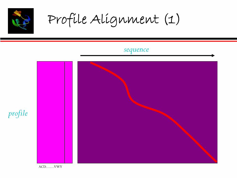
Profile Alignment (1)
ACD……VWY
sequence
profile

alignment of alignments• Sequence – Profile Alignment.• Profile – Profile Alignment.
Penalize gaps in conserved regions more heavily than gaps in more variable regions
Dynamic Programming. (same idea as in Pairwise Sequence Alignment)Optimal alignment in time O(a2l2)
a = alphabet size, l = sequence length
Profile Alignment (2)

Psi-Blast
Psi (Position Specific Iterated) is an automatic profile-like search
The program first performs a gapped blast search of the database. The information of the significant alignments is then used to construct a “position specific” score matrix. This matrix replaces the query sequence in the next round of database searching
The program may be iterated until no new significant are found
Summary
Diverse scope of bioinformatics
Pairwise sequence comparison
Multiple sequence comparison
Acknowledgement:
Prof Dong Xu, Chair, Dept of Computer science