computational statistics with application to...

The University of Texas at Austin, CS 395T, Spring 2008, Prof. William H. Press 1

Computational Statistics withApplication to Bioinformatics

Prof. William H. PressSpring Term, 2008

The University of Texas at Austin

Unit 20: Multidimensional Interpolation on Scattered Data


Unit 20: Multidimensional Interpolationon Scattered Data (Summary)

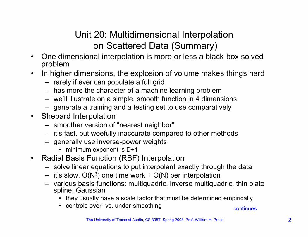
• One dimensional interpolation is more or less a black-box solved problem

• In higher dimensions, the explosion of volume makes things hard– rarely if ever can populate a full grid– has more the character of a machine learning problem– we’ll illustrate on a simple, smooth function in 4 dimensions– generate a training and a testing set to use comparatively

• Shepard Interpolation– smoother version of “nearest neighbor”– it’s fast, but woefully inaccurate compared to other methods– generally use inverse-power weights

• minimum exponent is D+1• Radial Basis Function (RBF) Interpolation

– solve linear equations to put interpolant exactly through the data– it’s slow, O(N3) one time work + O(N) per interpolation– various basis functions: multiquadric, inverse multiquadric, thin plate

spline, Gaussian• they usually have a scale factor that must be determined empirically• controls over- vs. under-smoothing continues


• Laplace Interpolation restores missing data values on a grid– solve Laplace’s equation with (interior) boundary conditions on known

values– implement by sparse linear method such as biconjugate gradient– can do remarkably well when as much as 90% of the values are missing

• Gaussian Process Regression (aka Linear Prediction, aka Kriging)– like Shepard and RBF, a weighted average of observed points– but the weights now determined by a statistical model, the variogram

• equivalent to estimating the covariance– can give error estimates– can be used both for interpolation (“honor the data”) and for filtering

(“smooth the data”)– it’s a kind of Wiener filtering in covariance space

• function covariance is the signal, noise covariance is the noise– cost is O(N3) one time work, O(N) per interpolation, O(N2) per variance

estimate


Interpolation on Scattered Data in Multidimensions

In 1-dimension, interpolation is basically a solved problem, OK to view as a black box (at least in this course):

pts = sort(rand(20,1));vals = exp(-3*pts.^2);ivals = interp1(pts,vals,[0:.001:1],'spline');tvals = exp(-3*[0:.001:1].^2);hist(ivals-tvals,50);

some smooth function of order unity

note scale

shape from oscillatory behavior of error term


In higher numbers of dimensions, especially >2, the explosion of volume makes things more interesting.

Rarely enough data for any kind of mesh.

Lots of near-ties for nearest neighbor points (none very near).

The problem is more like a machine learning problem:

Given a training set xi with “responses” yi, i = 1…NPredict y(x) for some new x


Let’s try some different methods on 500 data points in 4 dimensions.

5001/4 ≈ 4.7, so the data is sparse, but not ridiculous

testfun = @(x) 514.1890*exp(-2.0*norm(x-[.3 .3 .3 .3])) ...*x(1)*(1-x(1))*x(2)*(1-x(2))*x(3)*(1-x(3))*x(4)*(1-x(4));

[x1 x2] = meshgrid(0:.01:1,0:.01:1);z = arrayfun(@(s1,s2) testfun([s1 s2 .3 .3]), x1, x2);contour(z)

a Gaussian, off-center in the unit cube, and tapered to zero at its edges

z = arrayfun(@(s1,s2) testfun([s1 s2 .7 .7]), x1, x2);contour(z)


npts = 500;pts = cell(npts,1);for j=1:npts, pts{j} = rand(1,4); end;vals = cellfun(testfun,pts);hist(vals,50)

Generate training and testing sets of data.The points are chosen randomly in the unit cube.

tpts = cell(npts,1);for j=1:npts, tpts{j} = rand(1,4); end;tvals = cellfun(testfun,tpts);hist(tvals,50)

If you have only one sample of real data, you can test by leave-one-out, but that is a lot more expensive since you have to repeat the whole interpolation, including one-time work, each time.

most data points are where the function value is small

but a few find the peak of the Gaussian


Shepard Interpolation

The prediction is a weighted average of all the observed values, giving (much?) larger weights to those that are closest to the point of interest.

It’s a smoother version of “value of nearest neighbor” or “mean of few nearest neighbors”.

the power-law form has the advantage of being scale-free, so you don’t have to know a scale in the problem

In D dimensions, you’d better choose p ≥ D+1, otherwise you’re dominated by distant, not close, points: volume ~ no. of points ~ rD

Shepard interpolation is relatively fast, O(N) per interpolation.The problem is that it’s usually not very accurate.


function val = shepinterp(x,p,vals,pts)phi = cellfun(@(y) (norm(x-y)+1.e-40).^(-p), pts);val = (vals' * phi)./sum(phi);

shepvals = cellfun(@(x) shepinterp(x,6,vals,pts), tpts);plot(tvals,shepvals,'.')

hist(shepvals-tvals,50)

Shepard performance on our training/testing set:

note value of p

note biases


Want to see what happens if we choose too small a value of p for this D?

shepvals = cellfun(@(x) shepinterp(x,3,vals,pts), tpts);plot(tvals,shepvals,'.')hist(shepvals-tvals,50) small values are getting pulled up by

the (distant) peak

while peak values are getting pulled down

If you choose too large a value for p, you get ~ “value of nearest neighbor”


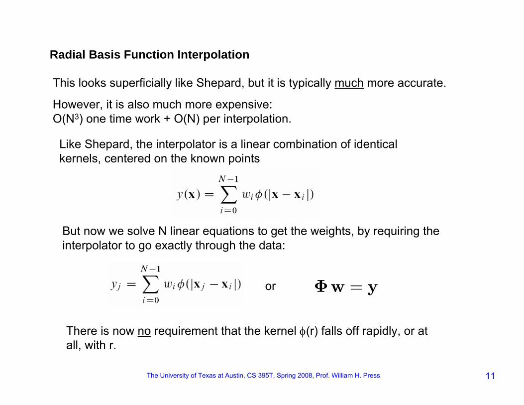
Radial Basis Function Interpolation

This looks superficially like Shepard, but it is typically much more accurate.

However, it is also much more expensive:O(N3) one time work + O(N) per interpolation.

Like Shepard, the interpolator is a linear combination of identical kernels, centered on the known points

But now we solve N linear equations to get the weights, by requiring the interpolator to go exactly through the data:

There is now no requirement that the kernel φ(r) falls off rapidly, or at all, with r.

or Φw = y


Commonly used Radial Basis Functions (RBFs)

“multiquadric”

you have to pick a scale factor

“inverse multiquadric”

“thin plate spline”

“Gaussian” Typically very sensitive to the choice of r0, and therefore less often used. (Remember the problems we had getting Gaussians to fit outliers!)

The choice of scale factor is a trade-off between over- and under-smoothing. (Bigger r0 gives more smoothing.) The optimal r0 is usually on the order of the typical nearest-neighbor distances.


r0 = 0.1;phi = @(x) sqrt(norm(x)^2+r0^2);phimat = zeros(npts,npts);for i=1:npts, for j=1:npts, phimat(i,j) = phi(pts{i}-pts{j}); end; end;wgts = phimat\vals;

valinterp = @(x) wgts' * cellfun(@(y) phi(norm(x-y)),pts);

ivals = cellfun(valinterp,tpts);hist(ivals-tvals,50)stdev = std(ivals-tvals)

Let’s try a multiquadric with r0 = 0.1

stdev =0.0145

Matlab “solve linear equations” operator!


function [stdev ivals] = TestAnRBF(phi,pts,vals,tpts,tvals)npts = numel(vals);phimat = zeros(npts,npts);for i=1:npts, for j=1:npts, phimat(i,j) = phi(pts{i}-pts{j}); end; end;wgts = phimat\vals;valinterp = @(x) wgts' * cellfun(@(y) phi(norm(x-y)),pts);ivals = cellfun(valinterp,tpts);stdev = std(ivals-tvals);

Automate the test process somewhat

r0 = 0.2;phi = @(x) sqrt(norm(x)^2+r0^2);[stdev ivals] = TestAnRBF(phi,pts,vals,tpts,tvals);stdevplot(tvals,ivals,'.')hist(ivals-tvals,50)

One test looks like

And the results are…

You have to redefine phi each time, because, in Matlab semantics, the value of r0 used is that at the time of definition, not execution.


r0 = 0.2 r0 = 0.6 r0 = 1.0

σ = 0.0099 σ = 0.0059 σ = 0.0104

so r0 ~ 0.6 is the optimal choice, and it’s not too sensitive


r0 = 0.6;phi = @(x) 1./sqrt(norm(x)^2+r0^2);[stdev ivals] = TestAnRBF(phi,pts,vals,tpts,tvals);stdevplot(tvals,ivals,'.')stdev =

0.0058

Try an inverse multiquadricr0 = 0.6

σ = 0.0058

(performance virtually identical to multiquadric on this example)

RBF interpolation is for interpolation on a smooth function, not for fitting a noisy data set.

By construction it exactly “honors the data”(meaning that it goes through the data points – it doesn’t smooth them).

If the data is in fact noisy, RBF will produce an interpolating function with spurious oscillations.


If y satisfies in any number of dimensions, then for any spherenot intersecting a boundary condition,

Laplace Interpolation is a specialized interpolation method for restoring missing data on a grid. It’s simple, but sometimes works astonishingly well.

Mean value theorem for solutions of Laplace’s equation (harmonic functions):

∇2y = 0

So Laplace’s equation is, in some sense, the perfect interpolator. It turns out to be the one that minimizes the integrated square of the gradient,

So the basic idea of Laplace interpolation is to setat every known data point, and solve at every unknown point.

1

area

Zsurface ω

y dω = y(center)


Lots of linear equations (one for each grid point)!

generic equation for an unknown pointnote that this is basically the mean value theorem

generic equation for a known point

lots of special cases:

There is exactly one equation for each grid point, so we can solve this as a giant (sparse!) linear system, e.g., by the bi-conjugate gradient method.

Surprise! It’s in NR3, as Laplace_interp, using Linbcg for the solution.


Easy to embed in a mex function for Matlab

#include "..\nr3_matlab.h"#include "linbcg.h"#include "interp_laplace.h“

/* Usage:outmatrix = laplaceinterp(inmatrix)

*/

Laplace_interp *mylap = NULL;

void mexFunction(int nlhs, mxArray *plhs[], int nrhs, const mxArray *prhs[]) {if (nrhs != 1 || nlhs != 1) throw("laplaceinterp.cpp: bad number of args");MatDoub ain(prhs[0]);MatDoub aout(ain.nrows(),ain.ncols(),plhs[0]);aout = ain; // matrix opmylap = new Laplace_interp(aout);mylap->solve();delete mylap;return;

}


IN = fopen('image-face.raw','r');face = flipud(reshape(fread(IN),256,256)');fclose(IN);bwcolormap = [0:1/256:1; 0:1/256:1; 0:1/256:1]';image(face)colormap(bwcolormap);axis('equal')

Let’s try it on our favorite face for filtering(But this is interpolation, not filtering: there is no noise!)


facemiss = face;ranface = rand(size(face));facemiss(ranface < 0.1) = 255;image(facemiss)colormap(bwcolormap)axis('equal')

delete a random 10% of pixels


facemiss(facemiss > 254) = 9.e99;newface = laplaceinterp(facemiss);image(newface)colormap(bwcolormap)axis('equal')

restore them by Laplace interpolation

pretty amazing!

this is the convention expected by laplaceinterp for missing data



delete a random 50% of pixels



restore them by Laplace interpolation

starting to see some degradation



delete a random 90% of pixels(well, it’s cheating a bit, because your eye can’t see the shades of grey in the glare of all that white)


This is a bit more fair…



still pretty amazing (e.g., would you have thought that the individual teeth were present in the sparse image?)

restore by Laplace interpolation


Linear Predictiona.k.a. Gaussian Process Regressiona.k.a. Kriging

What is “linear” about it, is that the interpolant is a linear combinationof the data y values, like Shepard interpolation (but on steroids!)

The weights, however, are highly nonlinear function of the x values.

They are based on a statistical model of the function’s smoothness instead of Shepard’s fixed (usually power law) radial functions. That’s where the “Gaussian” comes from, not from any use of Gaussian-shaped functions!

The weights can either honor the data (interpolation), or else smooth the data with a model of how much unsmoothness is due to noise (fitting).

The underlying (noise free) model need not even be smooth.

You can get error estimates.

This is actually pretty cool, but it’s concepts can be somewhat hard to understand the first time you see them, so bear with me!

Also, since this is spread out over three sections of NR3, the notation will keep hopping around (apologies!)

another idea too good to be invented only once!

Danie G. Krige


measured signal noise

an interpolated value

residual (we’ll try to minimize it)

using hyαnβi = 0 these quantities have values that come from the autocorrelation structure of the signal

this is the autocorrelation structure of the noise


Now take the derivative of the mean square residual w.r.t. the weights, and set it to zero. Immediately get

where

So,

This should remind you of Wiener filtering.In fact, it is Wiener filtering in the principal component basis:

So, this actually connects the lecture on PCA to the lecture on Wiener filtering!


Substituting back, we also get an estimate of the m.s. discrepancy

That’s the “basic version” of linear prediction.

Unfortunately, the basic version is missing a couple of important tweaks, both related to the fact that, viewed as a Gaussian process, y may not have a zero mean, and/or may not be stationary. (Actually these two possibilities are themselves closely related.)

Tweak 1: We should constrainThis is called “getting an unbiased estimator”.

Tweak 2: We should replace the covariance modelby an equivalent “variogram model”(If you square this out, you immediately see that the relation involveswhich is exactly the bad actor in a nonstationary process!)

Deriving the result is more than we want to do here, so we’ll jump to the answer. A (good content, but badly written) reference is Cressie, Statistics for Spatial Data.

Pβ d?β = 1

(yα − yβ)2

® y2α®hyαyβi


Most often, this is done by assuming that it is isotropic (spherically symmetric),Then you loop over all pairs of points for values from which to fit some parameterizedform like

The answer is (changing notation!):

1. Estimate the variogram

There’s an NR3 object for doing exactly this.

2. Define:

(The weird augmentation of 1’s and 0’s trickily imposes the unbiased estimator constraint don’t ask how!)

vij = v(|xi − xj |)

“power-law model”


3. Interpolate (as many times as you want) by

and (if you want) estimate the error by

Note that each interpolation (if you precompute the last two matrix factors) costs O(N), while each variance costs O(N2).

By the way, some other popular variogram models are

“exponential model”

“spherical model”


#include "..\nr3_matlab.h"#include "ludcmp.h"#include "krig.h"/* Matlab usage:

krig(x,y,err,beta) % err=0 for kriging interpolationyi = krig(xi)[yi yierr] = krig(xi)krig()

*/Powvargram *vgram = NULL;Krig<Powvargram> *krig = NULL;MatDoub xx;void cleanup() {

delete vgram;delete krig;xx.resize(1,1);

}void mexFunction(int nlhs, mxArray *plhs[], int nrhs, const mxArray *prhs[]) {

int ndim,npt,nerr,i,j;if (nlhs == 0 && nrhs == 4) { // constructor

if (krig) cleanup();MatDoub xtr(prhs[0]);VecDoub yy(prhs[1]);VecDoub err(prhs[2]);Doub beta = mxScalar<Doub>(prhs[3]);ndim = xtr.nrows(); // comes in as transpose!npt = xtr.ncols();nerr = err.size();xx.resize(npt,ndim);for (i=0;i<ndim;i++) for (j=0;j<npt;j++) xx[j][i] = xtr[i][j];vgram = new Powvargram(xx,yy,beta);if (nerr == npt) krig = new Krig<Powvargram>(xx,yy,*vgram,&err[0]);else krig = new Krig<Powvargram>(xx,yy,*vgram);

} else if (nlhs == 0 && nrhs == 0) { // destructorcleanup();

} else if (nlhs == 1 && nrhs == 1) { // interpolateif (!krig) throw("krig.cpp: must call constructor first");VecDoub xstar(prhs[0]);Doub &ystar = mxScalar<Doub>(plhs[0]);ystar = krig->interp(xstar);

} else if (nlhs == 2 && nrhs == 1) { // interpolate with errorif (!krig) throw("krig.cpp: must call constructor first");VecDoub xstar(prhs[0]);Doub &ystar = mxScalar<Doub>(plhs[0]);Doub &yerr = mxScalar<Doub>(plhs[1]);ystar = krig->interp(xstar,yerr);

} else {throw("krig.cpp: bad numbers of args");

}return;

}

I don’t think that Matlabhas Gaussian Process Regression (by any name), or at any rate I couldn’t find it. So, here is a wrapper for the NR3 class “Krig”.

Now it’s really easy:


ptsmat = zeros(npts,4);for j=1:npts, ptsmat(j,:) = pts{j}; end;for j=1:npts, tptsmat(j,:) = tpts{j}; end;

krig(ptsmat,vals,0,1.8);

kvals = zeros(npts,1);for j=1:npts, kvals(j) = krig(tpts{j}); end;plot(tvals,kvals,'.')

This is the exponent in the power-law model.1.5 is usually good. Closer to 2 for smoother functions.

Kriging results for our same 4-dimensional example:

std(kvals-tvals)hist(kvals-tvals,50)ans =

0.0140

about 3x worse than our best RBF, but waybetter than Shepard


How do the error estimates compare to the actual errors?

kerrs = zeros(npts,1);for j=1:npts, [kvals(j) kerrs(j)] = krig(tpts{j}); end;plot(abs(kvals-tvals),kerrs,'.')

Note that we don’t expect, or get, a point-by-point correlation, but only that the actual error is plausibly drawn from a Normal distribution with the indicated standard deviation.


The real power of Kriging is its ability to incorporate an error model, taking us past interpolation and to fitting / smoothing / filtering

interpolation: (σ’s = 0)


filtering: (σ’s ≠ 0) 1-σ error band should contain true curve ~2/3 of the time.

computational statistics with application to...

Documents