computer networks prof. ashok k agrawala © 2012 ashok agrawala set 6 · 2012-04-17 · ip service:...
TRANSCRIPT

CMSC 417
Computer Networks
Prof. Ashok K Agrawala
© 2012 Ashok Agrawala
Set 6
April 12 CMSC417 Set 6 1
The Network Layer
April 12 CMSC417 Set 6 2
Network Layer Design Isues
• Store-and-Forward Packet Switching
• Services Provided to the Transport Layer
• Implementation of Connectionless Service
• Implementation of Connection-Oriented Service
• Comparison of Virtual-Circuit and Datagram Subnets
April 12 CMSC417 Set 6 3
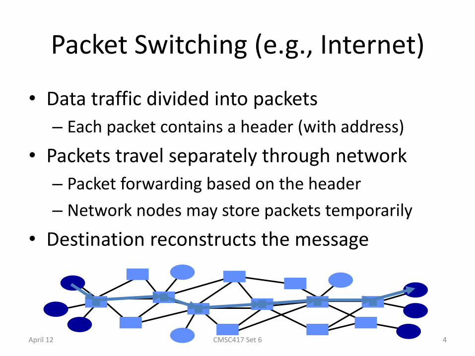
Packet Switching (e.g., Internet)
• Data traffic divided into packets
– Each packet contains a header (with address)
• Packets travel separately through network
– Packet forwarding based on the header
– Network nodes may store packets temporarily
• Destination reconstructs the message
April 12 CMSC417 Set 6 4
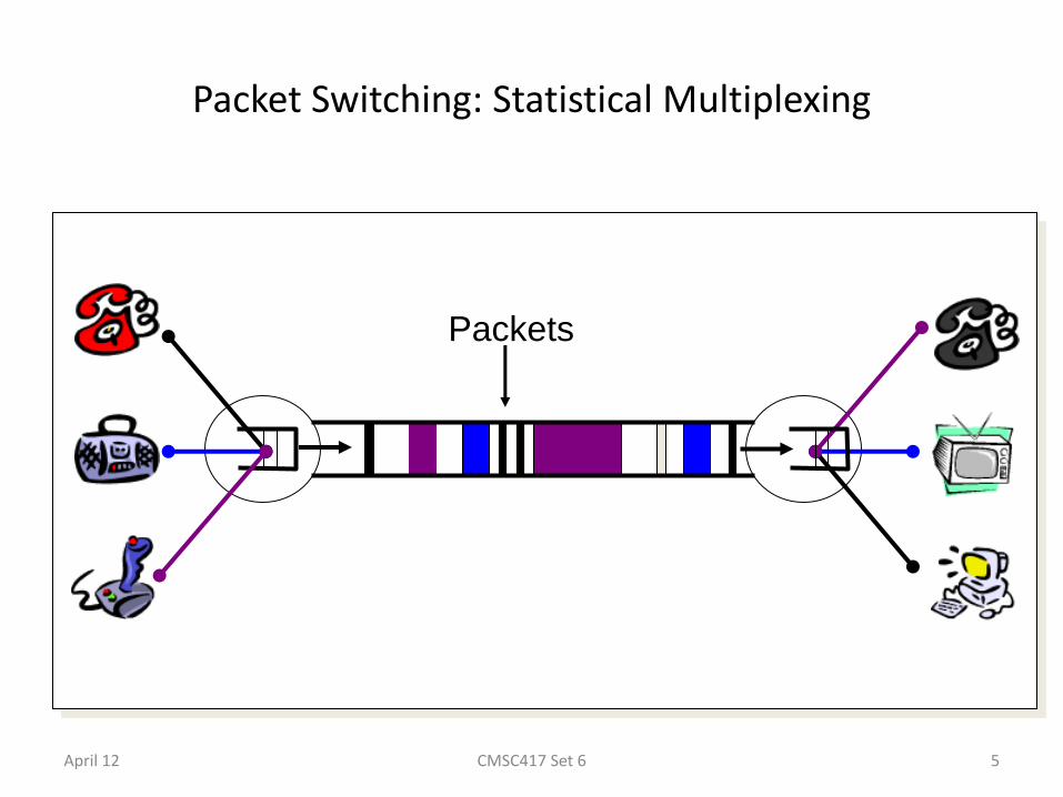
Packet Switching: Statistical Multiplexing
April 12 CMSC417 Set 6 5
Packets
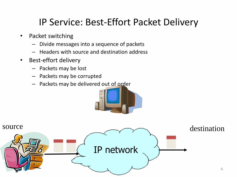
IP Service: Best-Effort Packet Delivery
April 12 CMSC417 Set 6 6
• Packet switching – Divide messages into a sequence of packets
– Headers with source and destination address
• Best-effort delivery – Packets may be lost
– Packets may be corrupted
– Packets may be delivered out of order
source destination
IP network
IP Service Model: Why Packets?
• Data traffic is bursty – Logging in to remote machines – Exchanging e-mail messages
• Don’t want to waste reserved bandwidth – No traffic exchanged during idle periods
• Better to allow multiplexing – Different transfers share access to same links
• Packets can be delivered by most anything – RFC 2549: IP over Avian Carriers (aka birds)
• … still, packet switching can be inefficient – Extra header bits on every packet
April 12 CMSC417 Set 6 7
IP Service Model: Why Best-Effort?
• IP means never having to say you’re sorry…
– Don’t need to reserve bandwidth and memory
– Don’t need to do error detection & correction
– Don’t need to remember from one packet to next
• Easier to survive failures
– Transient disruptions are okay during failover
• … but, applications do want efficient, accurate transfer of data in order, in a timely fashion
April 12 CMSC417 Set 6 8
IP Service: Best-Effort is Enough
• No error detection or correction – Higher-level protocol can provide error checking
• Successive packets may not follow the same path – Not a problem as long as packets reach the destination
• Packets can be delivered out-of-order – Receiver can put packets back in order (if necessary)
• Packets may be lost or arbitrarily delayed – Sender can send the packets again (if desired)
• No network congestion control (beyond “drop”) – Sender can slow down in response to loss or delay
April 12 CMSC417 Set 6 9
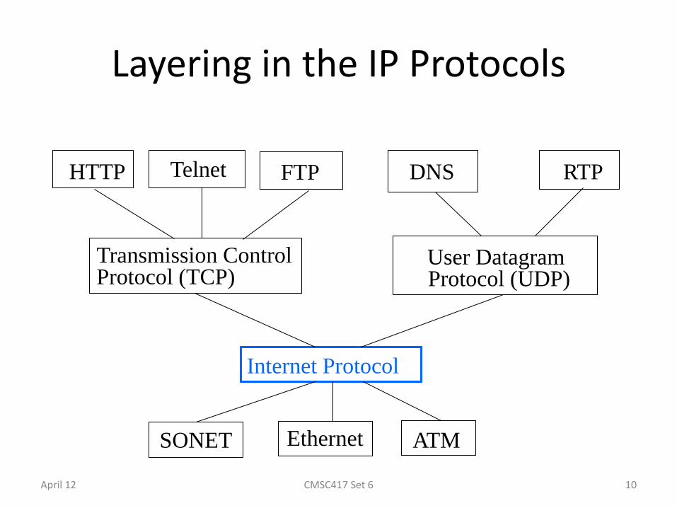
Layering in the IP Protocols
April 12 CMSC417 Set 6 10
Internet Protocol
Transmission Control Protocol (TCP)
User Datagram Protocol (UDP)
Telnet HTTP
SONET ATM Ethernet
RTP DNS FTP
History: Why IP Packets?
• IP proposed in the early 1970s – Defense Advanced Research Project Agency (DARPA)
• Goal: connect existing networks – To develop an effective technique for multiplexed utilization of
existing interconnected networks – E.g., connect packet radio networks to the ARPAnet
• Motivating applications – Remote login to server machines – Inherently bursty traffic with long silent periods
• Prior ARPAnet experience with packet switching – Previous DARPA project – Demonstrated store-and-forward packet switching
April 12 CMSC417 Set 6 11
Other Main Driving Goals (In Order)
• Communication should continue despite failures
– Survive equipment failure or physical attack
– Traffic between two hosts continue on another path
• Support multiple types of communication services
– Differing requirements for speed, latency, & reliability
– Bidirectional reliable delivery vs. message service
• Accommodate a variety of networks
– Both military and commercial facilities
– Minimize assumptions about the underlying network
April 12 CMSC417 Set 6 12
Other Driving Goals, Somewhat Met
• Permit distributed management of resources – Nodes managed by different institutions – … though this is still rather challenging
• Cost-effectiveness – Statistical multiplexing through packet switching – … though packet headers and retransmissions wasteful
• Ease of attaching new hosts – Standard implementations of end-host protocols – … though still need a fair amount of end-host software
• Accountability for use of resources – Monitoring functions in the nodes – … though this is still fairly limited and immature
April 12 CMSC417 Set 6 13

IP Packet Structure
April 12 CMSC417 Set 6 14
4-bit
Version
4-bit
Header
Length
8-bit
Type of Service
(TOS)
16-bit Total Length (Bytes)
16-bit Identification 3-bit
Flags 13-bit Fragment Offset
8-bit Time to
Live (TTL) 8-bit Protocol 16-bit Header Checksum
32-bit Source IP Address
32-bit Destination IP Address
Options (if any)
Payload
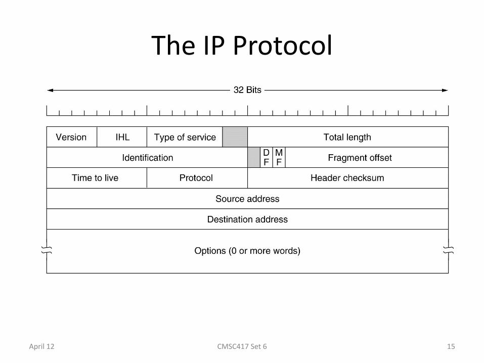
The IP Protocol
The IPv4 (Internet Protocol) header.
April 12 CMSC417 Set 6 15
IP Packet Header Fields
• Version number (4 bits) – Indicates the version of the IP protocol
– Necessary to know what other fields to expect
– Typically “4” (for IPv4), and sometimes “6” (for IPv6)
• Header length (4 bits) – Number of 32-bit words in the header
– Typically “5” (for a 20-byte IPv4 header)
– Can be more when “IP options” are used
• Type-of-Service (8 bits) – Allow packets to be treated differently based on needs
– E.g., low delay for audio, high bandwidth for bulk transfer
April 12 CMSC417 Set 6 16
IP Packet Header Fields (Continued)
• Total length (16 bits) – Number of bytes in the packet
– Maximum size is 63,535 bytes (216 -1)
– … though underlying links may impose harder limits
• Fragmentation information (32 bits) – Packet identifier, flags, and fragment offset
– Supports dividing a large IP packet into fragments
– … in case a link cannot handle a large IP packet
• Time-To-Live (8 bits) – Used to identify packets stuck in forwarding loops
– … and eventually discard them from the network
April 12 CMSC417 Set 6 17
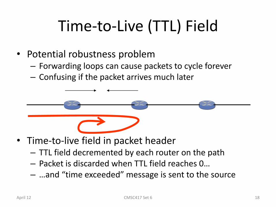
Time-to-Live (TTL) Field
• Potential robustness problem – Forwarding loops can cause packets to cycle forever – Confusing if the packet arrives much later
• Time-to-live field in packet header – TTL field decremented by each router on the path – Packet is discarded when TTL field reaches 0… – …and “time exceeded” message is sent to the source
April 12 CMSC417 Set 6 18

Application of TTL in Traceroute
• Time-To-Live field in IP packet header – Source sends a packet with a TTL of n
– Each router along the path decrements the TTL
– “TTL exceeded” sent when TTL reaches 0
• Traceroute tool exploits this TTL behavior
April 12 CMSC417 Set 6 19
source destination
TTL=1
Time
exceeded
TTL=2
Send packets with TTL=1, 2, … and record source of “time exceeded” message
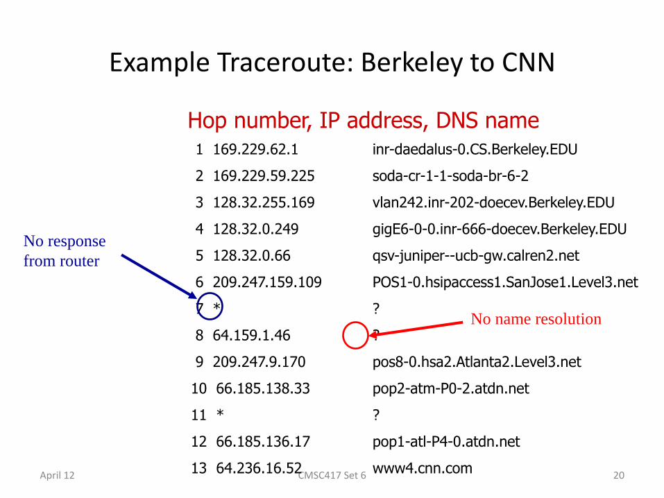
Example Traceroute: Berkeley to CNN
April 12 CMSC417 Set 6 20
1 169.229.62.1
2 169.229.59.225
3 128.32.255.169
4 128.32.0.249
5 128.32.0.66
6 209.247.159.109
7 *
8 64.159.1.46
9 209.247.9.170
10 66.185.138.33
11 *
12 66.185.136.17
13 64.236.16.52
Hop number, IP address, DNS name inr-daedalus-0.CS.Berkeley.EDU
soda-cr-1-1-soda-br-6-2
vlan242.inr-202-doecev.Berkeley.EDU
gigE6-0-0.inr-666-doecev.Berkeley.EDU
qsv-juniper--ucb-gw.calren2.net
POS1-0.hsipaccess1.SanJose1.Level3.net
?
?
pos8-0.hsa2.Atlanta2.Level3.net
pop2-atm-P0-2.atdn.net
?
pop1-atl-P4-0.atdn.net
www4.cnn.com
No response
from router
No name resolution
Try Running Traceroute Yourself
• On UNIX machine – Traceroute
– E.g., “traceroute www.cnn.com” or “traceroute 12.1.1.1”
• On Windows machine – Tracert
– E.g., “tracert www.cnn.com” or “tracert 12.1.1.1”
• Common uses of traceroute – Discover the topology of the Internet
– Debug performance and reachability problems
April 12 CMSC417 Set 6 21
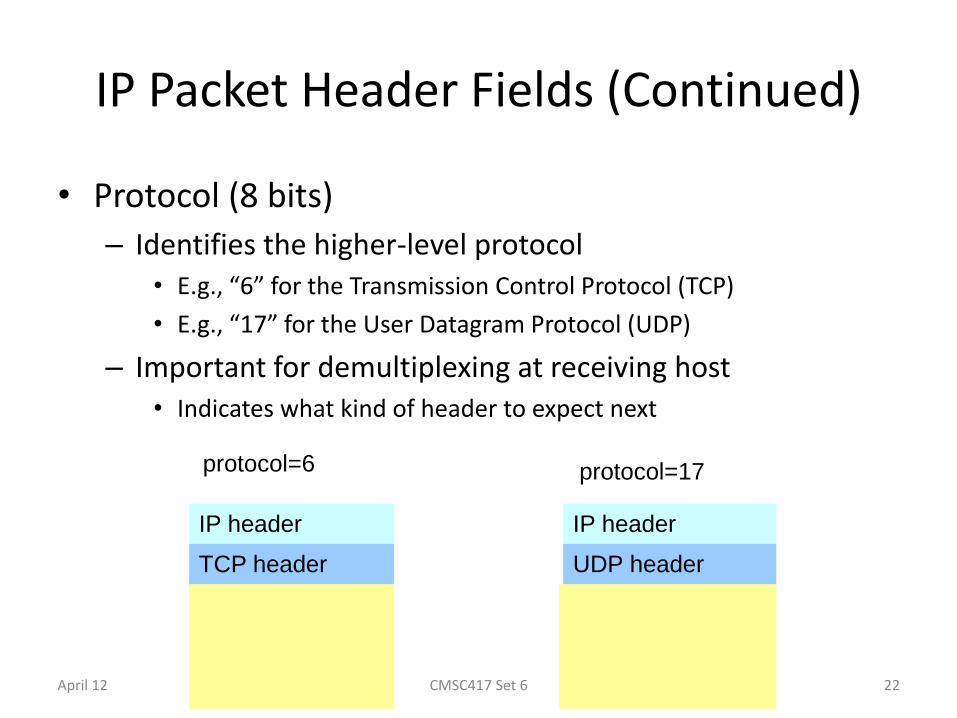
IP Packet Header Fields (Continued)
• Protocol (8 bits)
– Identifies the higher-level protocol • E.g., “6” for the Transmission Control Protocol (TCP)
• E.g., “17” for the User Datagram Protocol (UDP)
– Important for demultiplexing at receiving host • Indicates what kind of header to expect next
April 12 CMSC417 Set 6 22
IP header IP header
TCP header UDP header
protocol=6 protocol=17

IP Packet Header Fields (Continued)
• Checksum (16 bits)
– Sum of all 16-bit words in the IP packet header
– If any bits of the header are corrupted in transit
– … the checksum won’t match at receiving host
– Receiving host discards corrupted packets • Sending host will retransmit the packet, if needed
April 12 CMSC417 Set 6 23
134
+ 212
= 346
134
+ 216
= 350
Mismatch!
IP Packet Header (Continued)
• Two IP addresses – Source IP address (32 bits) – Destination IP address (32 bits)
• Destination address – Unique identifier for the receiving host – Allows each node to make forwarding decisions
• Source address – Unique identifier for the sending host – Recipient can decide whether to accept packet – Enables recipient to send a reply back to source
April 12 CMSC417 Set 6 24
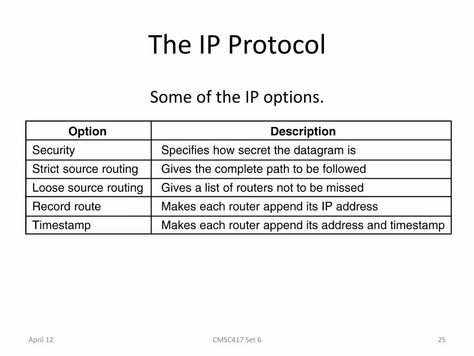
The IP Protocol
Some of the IP options.
5-54
April 12 CMSC417 Set 6 25
What if the Source Lies?
• Source address should be the sending host – But, who’s checking, anyway? – You could send packets with any source you want
• Why would someone want to do this? – Launch a denial-of-service attack
• Send excessive packets to the destination • … to overload the node, or the links leading to the node
– Evade detection by “spoofing” • But, the victim could identify you by the source address • So, you can put someone else’s source address in the packets
– Also, an attack against the spoofed host • Spoofed host is wrongly blamed • Spoofed host may receive return traffic from the receiver
April 12 CMSC417 Set 6 26
IP Addressing and Forwarding
April 12 27 CMSC417 Set 6
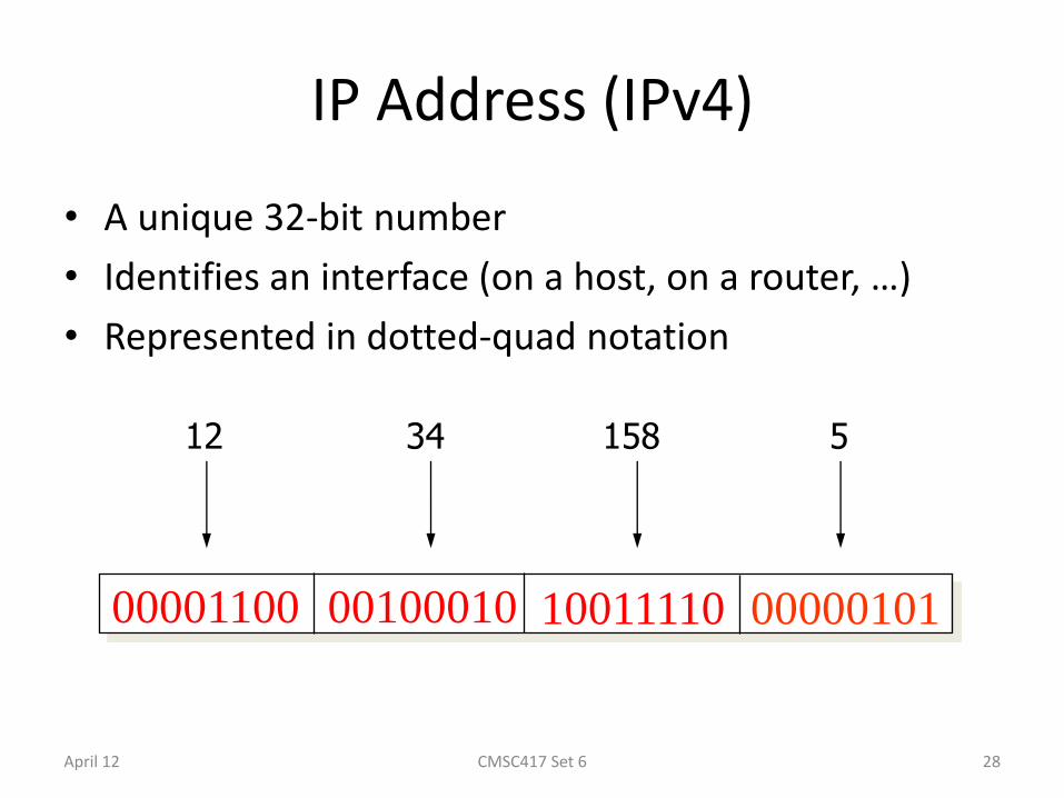
IP Address (IPv4)
• A unique 32-bit number
• Identifies an interface (on a host, on a router, …)
• Represented in dotted-quad notation
28
00001100 00100010 10011110 00000101
12 34 158 5
April 12 CMSC417 Set 6

Grouping Related Hosts
• The Internet is an “inter-network”
– Used to connect networks together, not hosts
– Needs a way to address a network (i.e., group of hosts)
29
host host host
LAN 1
... host host host
LAN 2
...
router router router WAN WAN
LAN = Local Area Network
WAN = Wide Area Network April 12 CMSC417 Set 6
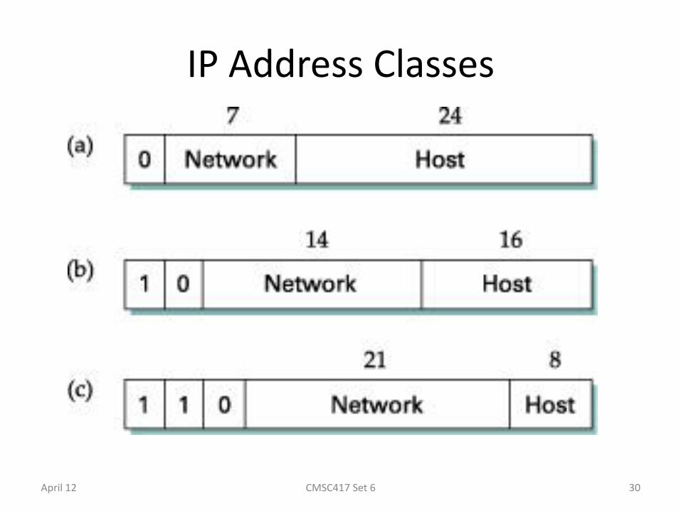
IP Address Classes
April 12 CMSC417 Set 6 30
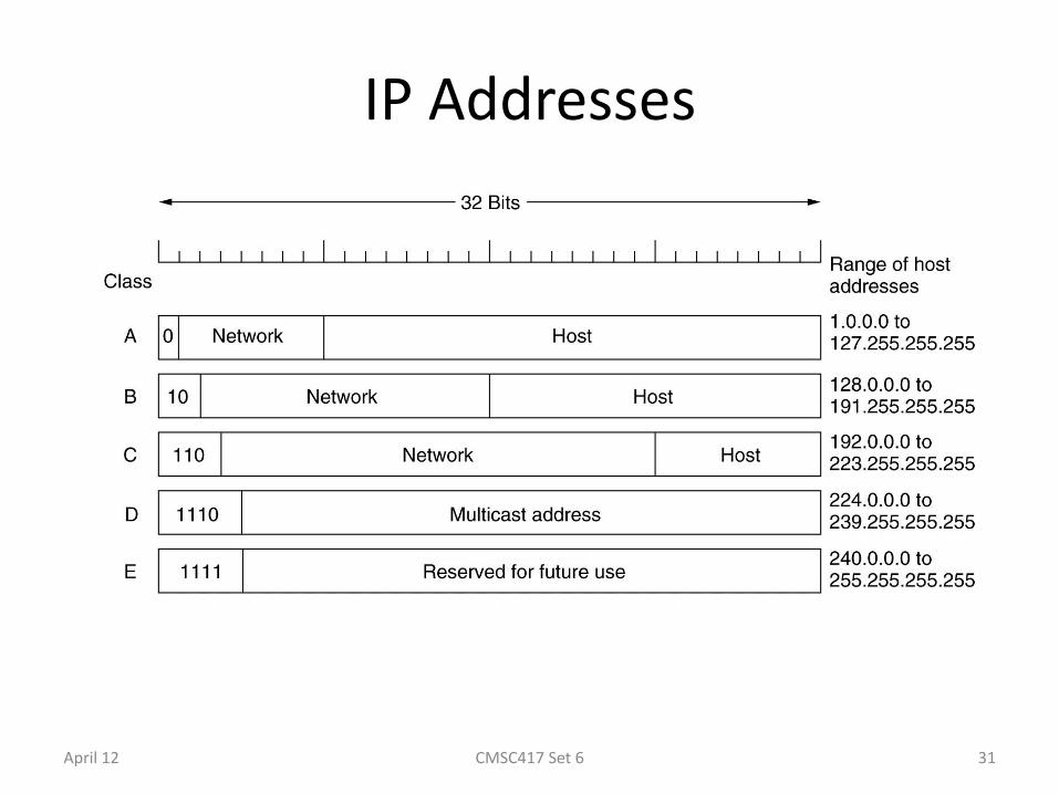
IP Addresses
IP address formats.
April 12 CMSC417 Set 6 31

IP Addresses (2)
Special IP addresses.
April 12 CMSC417 Set 6 32

Subnets
A campus network consisting of LANs for various departments.
April 12 CMSC417 Set 6 33
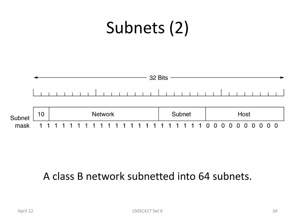
Subnets (2)
A class B network subnetted into 64 subnets.
April 12 CMSC417 Set 6 34
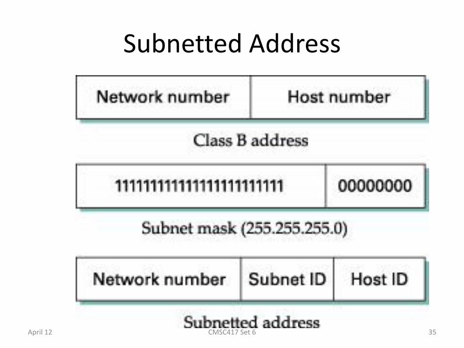
Subnetted Address
April 12 CMSC417 Set 6 35
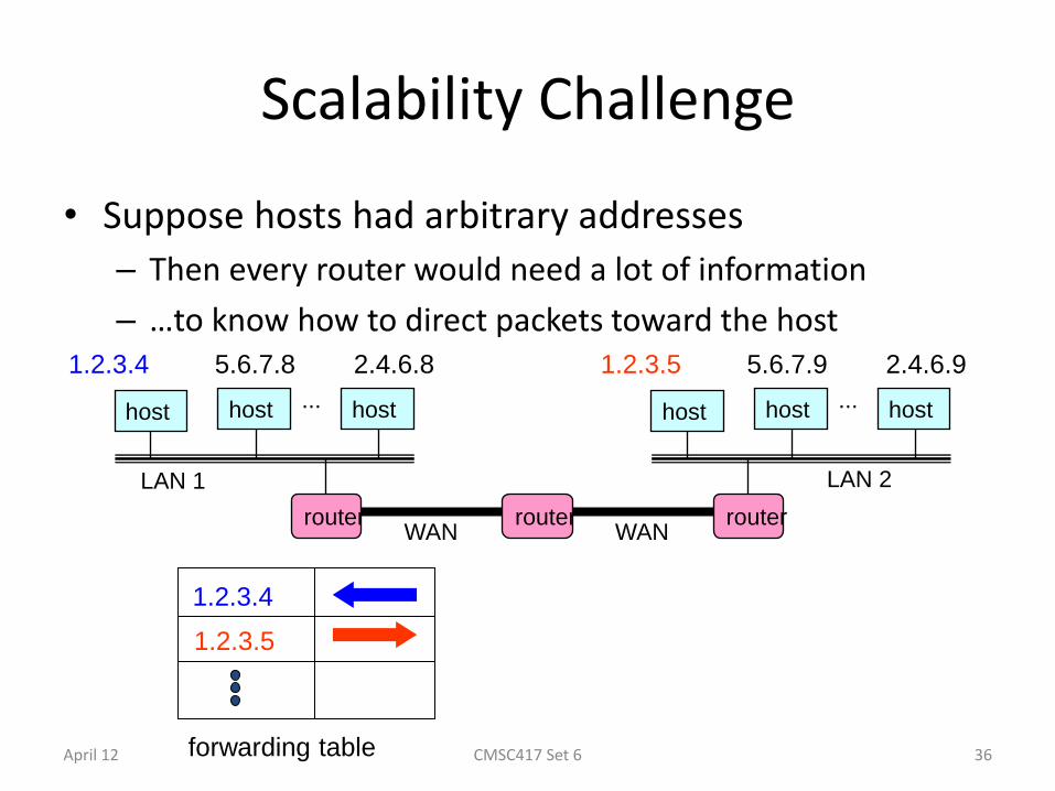
Scalability Challenge
• Suppose hosts had arbitrary addresses
– Then every router would need a lot of information
– …to know how to direct packets toward the host
36
host host host
LAN 1
... host host host
LAN 2
...
router router router WAN WAN
1.2.3.4 5.6.7.8 2.4.6.8 1.2.3.5 5.6.7.9 2.4.6.9
1.2.3.4
1.2.3.5
forwarding table April 12 CMSC417 Set 6
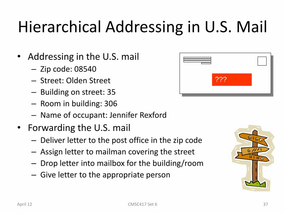
Hierarchical Addressing in U.S. Mail
• Addressing in the U.S. mail – Zip code: 08540
– Street: Olden Street
– Building on street: 35
– Room in building: 306
– Name of occupant: Jennifer Rexford
• Forwarding the U.S. mail – Deliver letter to the post office in the zip code
– Assign letter to mailman covering the street
– Drop letter into mailbox for the building/room
– Give letter to the appropriate person
37
???
April 12 CMSC417 Set 6
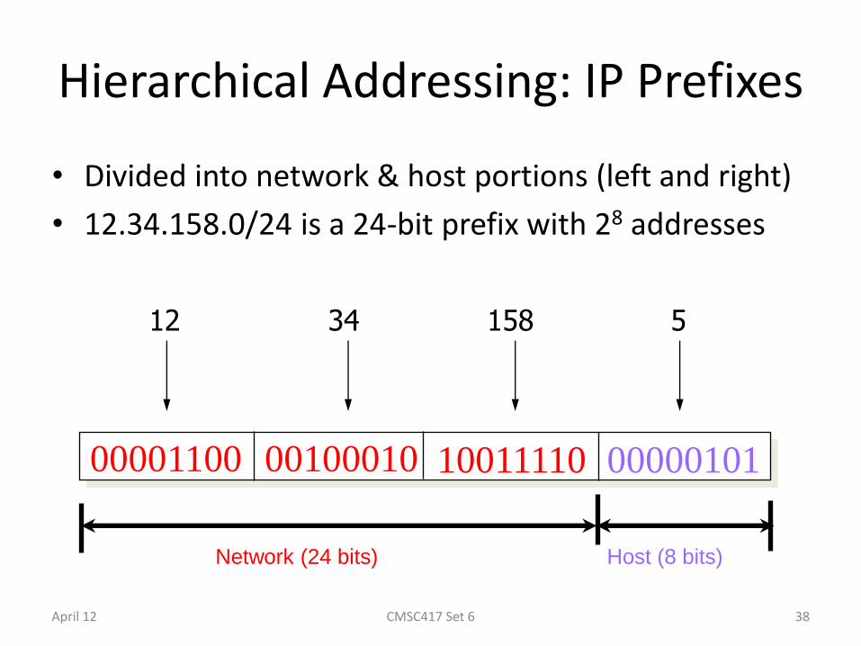
Hierarchical Addressing: IP Prefixes
• Divided into network & host portions (left and right)
• 12.34.158.0/24 is a 24-bit prefix with 28 addresses
38
00001100 00100010 10011110 00000101
Network (24 bits) Host (8 bits)
12 34 158 5
April 12 CMSC417 Set 6
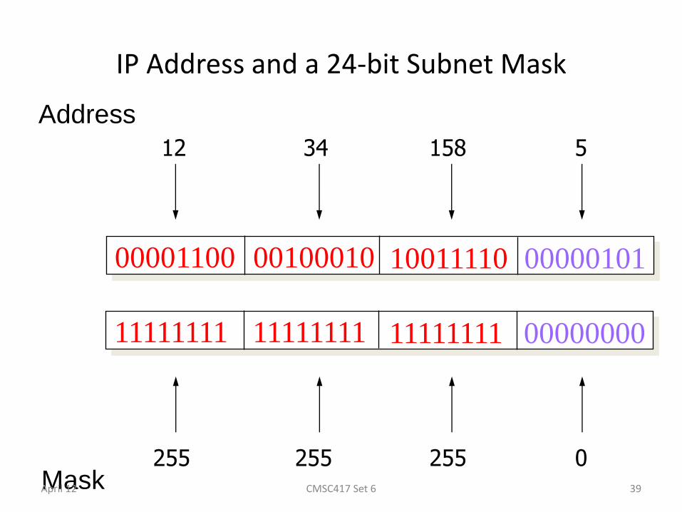
IP Address and a 24-bit Subnet Mask
39
00001100 00100010 10011110 00000101
12 34 158 5
11111111 11111111 11111111 00000000
255 255 255 0
Address
Mask April 12 CMSC417 Set 6
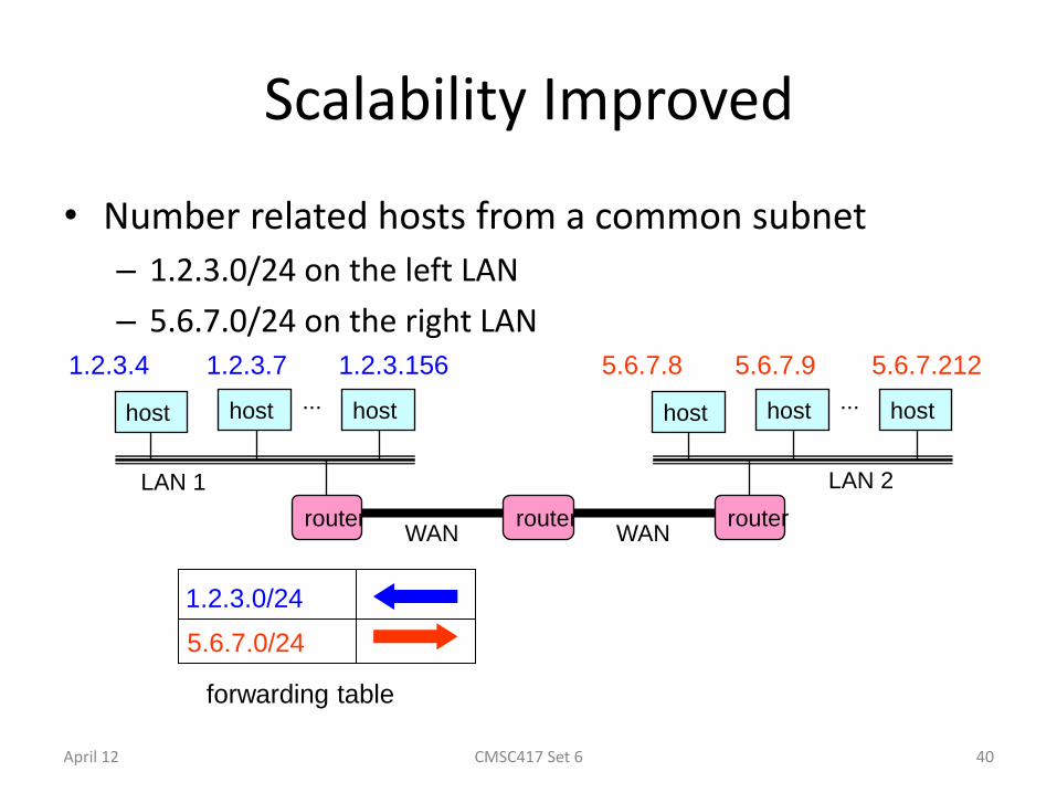
Scalability Improved
• Number related hosts from a common subnet
– 1.2.3.0/24 on the left LAN
– 5.6.7.0/24 on the right LAN
40
host host host
LAN 1
... host host host
LAN 2
...
router router router WAN WAN
1.2.3.4 1.2.3.7 1.2.3.156 5.6.7.8 5.6.7.9 5.6.7.212
1.2.3.0/24
5.6.7.0/24
forwarding table
April 12 CMSC417 Set 6
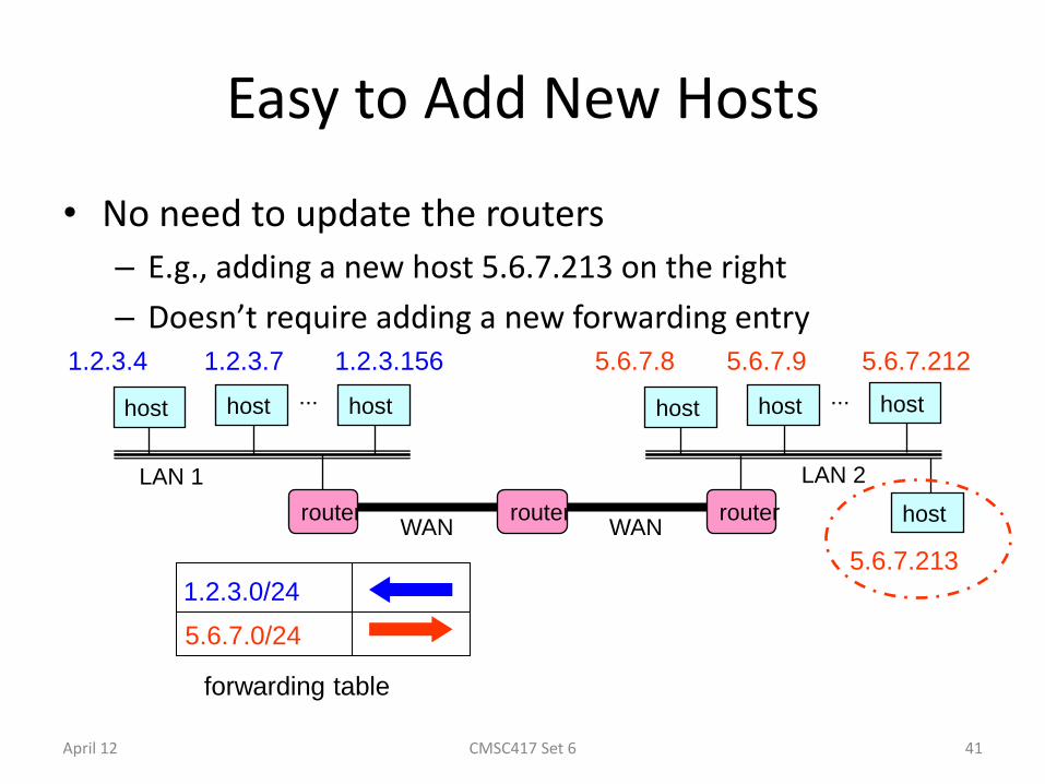
Easy to Add New Hosts
• No need to update the routers
– E.g., adding a new host 5.6.7.213 on the right
– Doesn’t require adding a new forwarding entry
41
host host host
LAN 1
... host host host
LAN 2
...
router router router WAN WAN
1.2.3.4 1.2.3.7 1.2.3.156 5.6.7.8 5.6.7.9 5.6.7.212
1.2.3.0/24
5.6.7.0/24
forwarding table
host
5.6.7.213
April 12 CMSC417 Set 6
Address Allocation
42 April 12 CMSC417 Set 6

Classful Addressing
• In the olden days, only fixed allocation sizes – Class A: 0*
• Very large /8 blocks (e.g., MIT has 18.0.0.0/8) – Class B: 10*
• Large /16 blocks (e.g,. Princeton has 128.112.0.0/16) – Class C: 110*
• Small /24 blocks (e.g., AT&T Labs has 192.20.225.0/24) – Class D: 1110*
• Multicast groups – Class E: 11110*
• Reserved for future use
• This is why folks use dotted-quad notation!
43 April 12 CMSC417 Set 6
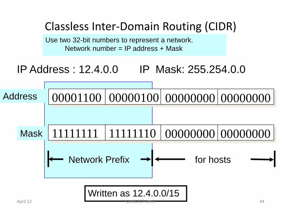
Classless Inter-Domain Routing (CIDR)
44
IP Address : 12.4.0.0 IP Mask: 255.254.0.0
00001100 00000100 00000000 00000000
11111111 11111110 00000000 00000000
Address
Mask
for hosts Network Prefix
Use two 32-bit numbers to represent a network.
Network number = IP address + Mask
Written as 12.4.0.0/15 April 12 CMSC417 Set 6
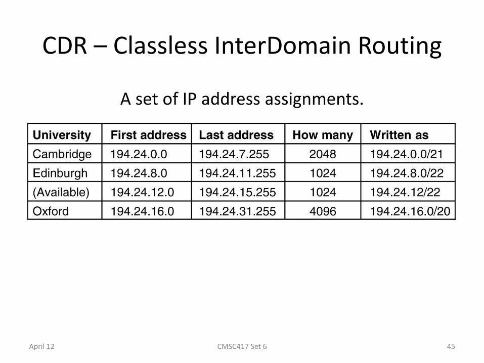
CDR – Classless InterDomain Routing
A set of IP address assignments.
5-59
April 12 CMSC417 Set 6 45

CIDR: Hierarchal Address Allocation
46
12.0.0.0/8
12.0.0.0/16
12.254.0.0/16
12.1.0.0/16
12.2.0.0/16
12.3.0.0/16
:
:
:
12.3.0.0/24 12.3.1.0/24
:
: 12.3.254.0/24
12.253.0.0/19 12.253.32.0/19 12.253.64.0/19
12.253.96.0/19 12.253.128.0/19 12.253.160.0/19
:
:
:
• Prefixes are key to Internet scalability – Address allocated in contiguous chunks (prefixes)
– Routing protocols and packet forwarding based on prefixes
– Today, routing tables contain ~150,000-200,000 prefixes
April 12 CMSC417 Set 6

Scalability: Address Aggregation
47
Provider is given 201.10.0.0/21
201.10.0.0/22 201.10.4.0/24 201.10.5.0/24 201.10.6.0/23
Provider
Routers in the rest of the Internet just need to know how to
reach 201.10.0.0/21. The provider can direct the IP
packets to the appropriate customer. April 12 CMSC417 Set 6
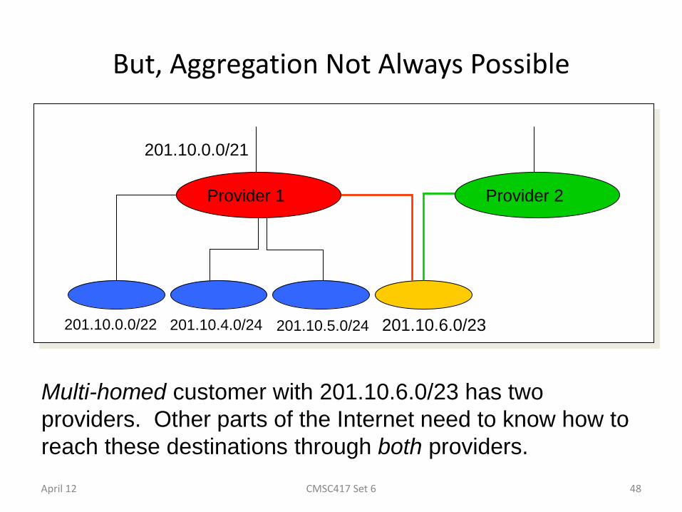
But, Aggregation Not Always Possible
48
201.10.0.0/21
201.10.0.0/22 201.10.4.0/24 201.10.5.0/24 201.10.6.0/23
Provider 1 Provider 2
Multi-homed customer with 201.10.6.0/23 has two
providers. Other parts of the Internet need to know how to
reach these destinations through both providers.
April 12 CMSC417 Set 6
Scalability Through Hierarchy
• Hierarchical addressing – Critical for scalable system
– Don’t require everyone to know everyone else
– Reduces amount of updating when something changes
• Non-uniform hierarchy – Useful for heterogeneous networks of different sizes
– Initial class-based addressing was far too coarse
– Classless InterDomain Routing (CIDR) helps
• Next few slides – History of the number of globally-visible prefixes
– Plots are # of prefixes vs. time
49 April 12 CMSC417 Set 6
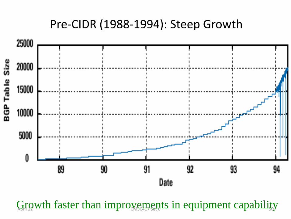
Pre-CIDR (1988-1994): Steep Growth
50 Growth faster than improvements in equipment capability April 12 CMSC417 Set 6
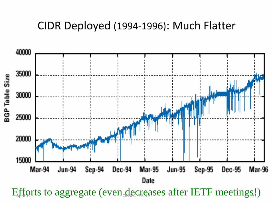
CIDR Deployed (1994-1996): Much Flatter
51 Efforts to aggregate (even decreases after IETF meetings!) April 12 CMSC417 Set 6
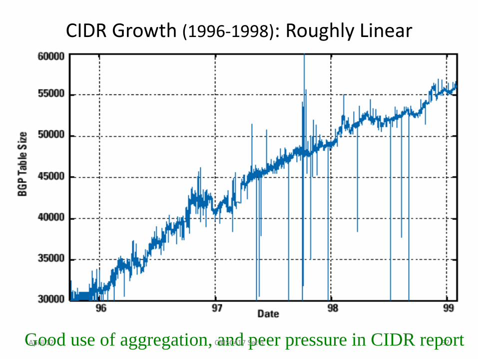
CIDR Growth (1996-1998): Roughly Linear
52 Good use of aggregation, and peer pressure in CIDR report April 12 CMSC417 Set 6
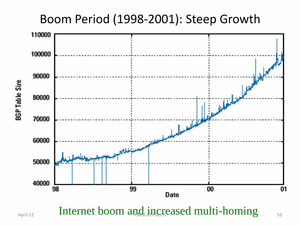
Boom Period (1998-2001): Steep Growth
53 Internet boom and increased multi-homing April 12 CMSC417 Set 6
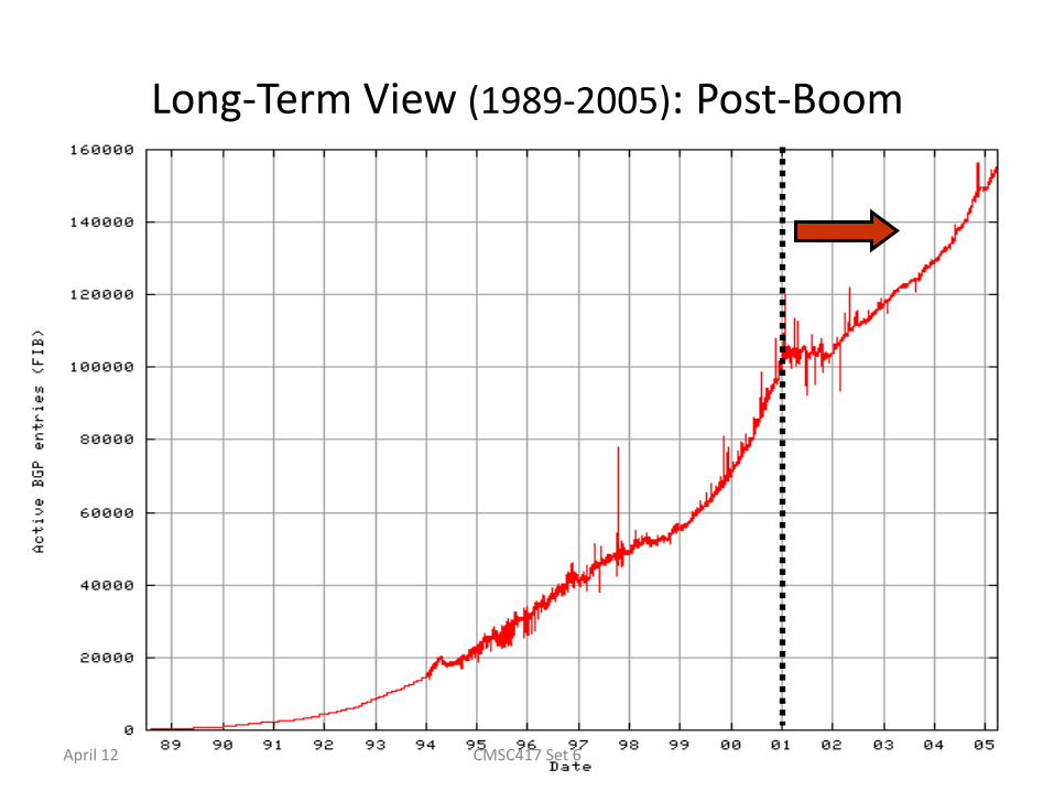
Long-Term View (1989-2005): Post-Boom
54 April 12 CMSC417 Set 6

Obtaining a Block of Addresses
• Separation of control – Prefix: assigned to an institution – Addresses: assigned by the institution to their nodes
• Who assigns prefixes? – Internet Corporation for Assigned Names and Numbers
• Allocates large address blocks to Regional Internet Registries
– Regional Internet Registries (RIRs) • E.g., ARIN (American Registry for Internet Numbers) • Allocates address blocks within their regions • Allocated to Internet Service Providers and large institutions
– Internet Service Providers (ISPs) • Allocate address blocks to their customers • Who may, in turn, allocate to their customers…
55 April 12 CMSC417 Set 6
Figuring Out Who Owns an Address
• Address registries – Public record of address allocations
– Internet Service Providers (ISPs) should update when giving addresses to customers
– However, records are notoriously out-of-date
• Ways to query – UNIX: “whois –h whois.arin.net 128.8.130.75”
– http://www.arin.net/whois/
– http://www.geektools.com/whois.php
– …
56 April 12 CMSC417 Set 6
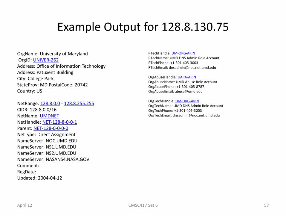
Example Output for 128.8.130.75
OrgName: University of Maryland OrgID: UNIVER-262 Address: Office of Information Technology Address: Patuxent Building City: College Park StateProv: MD PostalCode: 20742 Country: US NetRange: 128.8.0.0 - 128.8.255.255 CIDR: 128.8.0.0/16 NetName: UMDNET NetHandle: NET-128-8-0-0-1 Parent: NET-128-0-0-0-0 NetType: Direct Assignment NameServer: NOC.UMD.EDU NameServer: NS1.UMD.EDU NameServer: NS2.UMD.EDU NameServer: NASANS4.NASA.GOV Comment: RegDate: Updated: 2004-04-12
RTechHandle: UM-ORG-ARIN RTechName: UMD DNS Admin Role Account RTechPhone: +1-301-405-3003 RTechEmail: [email protected] OrgAbuseHandle: UARA-ARIN OrgAbuseName: UMD Abuse Role Account OrgAbusePhone: +1-301-405-8787 OrgAbuseEmail: [email protected] OrgTechHandle: UM-ORG-ARIN OrgTechName: UMD DNS Admin Role Account OrgTechPhone: +1-301-405-3003 OrgTechEmail: [email protected]
April 12 CMSC417 Set 6 57
Are 32-bit Addresses Enough?
• Not all that many unique addresses – 232 = 4,294,967,296 (just over four billion) – Plus, some are reserved for special purposes – And, addresses are allocated in larger blocks
• And, many devices need IP addresses – Computers, PDAs, routers, tanks, toasters, …
• Long-term solution: a larger address space – IPv6 has 128-bit addresses (2128 = 3.403 × 1038)
• Short-term solutions: limping along with IPv4 – Private addresses – Network address translation (NAT) – Dynamically-assigned addresses (DHCP)
58 April 12 CMSC417 Set 6
Hard Policy Questions
• How much address space per geographic region? – Equal amount per country? – Proportional to the population? – What about addresses already allocated?
• Address space portability? – Keep your address block when you change providers? – Pro: avoid having to renumber your equipment – Con: reduces the effectiveness of address aggregation
• Keeping the address registries up to date? – What about mergers and acquisitions? – Delegation of address blocks to customers? – As a result, the registries are horribly out of date
59 April 12 CMSC417 Set 6
Packet Forwarding
April 12 CMSC417 Set 6 60
Hop-by-Hop Packet Forwarding
• Each router has a forwarding table – Maps destination addresses…
– … to outgoing interfaces
• Upon receiving a packet – Inspect the destination IP address in the header
– Index into the table
– Determine the outgoing interface
– Forward the packet out that interface
• Then, the next router in the path repeats – And the packet travels along the path to the destination
61 April 12 CMSC417 Set 6

Separate Table Entries Per Address
• If a router had a forwarding entry per IP address
– Match destination address of incoming packet
– … to the forwarding-table entry
– … to determine the outgoing interface
62
host host host
LAN 1
... host host host
LAN 2
...
router router router WAN WAN
1.2.3.4 5.6.7.8 2.4.6.8 1.2.3.5 5.6.7.9 2.4.6.9
1.2.3.4
1.2.3.5
forwarding table April 12 CMSC417 Set 6

Separate Entry Per 24-bit Prefix
• If the router had an entry per 24-bit prefix
– Look only at the top 24 bits of the destination address
– Index into the table to determine the next-hop interface
63
host host host
LAN 1
... host host host
LAN
...
router router router WAN WAN
1.2.3.4 1.2.3.7 1.2.3.156 5.6.7.8 5.6.7.9 5.6.7.212
1.2.3.0/24
5.6.7.0/24
forwarding table April 12 CMSC417 Set 6

Separate Entry Classful Address
• If the router had an entry per classful prefix – Mixture of Class A, B, and C addresses
– Depends on the first couple of bits of the destination
• Identify the mask automatically from the address – First bit of 0: class A address (/8)
– First two bits of 10: class B address (/16)
– First three bits of 110: class C address (/24)
• Then, look in the forwarding table for the match – E.g., 1.2.3.4 maps to 1.2.3.0/24
– Then, look up the entry for 1.2.3.0/24
– … to identify the outgoing interface
64 April 12 CMSC417 Set 6
CIDR Makes Packet Forwarding Harder
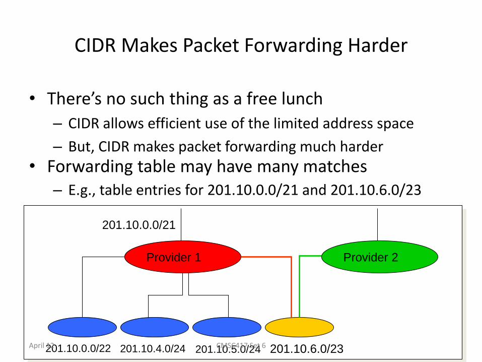
• There’s no such thing as a free lunch
– CIDR allows efficient use of the limited address space
– But, CIDR makes packet forwarding much harder
• Forwarding table may have many matches – E.g., table entries for 201.10.0.0/21 and 201.10.6.0/23
– The IP address 201.10.6.17 would match both!
65
201.10.0.0/21
201.10.0.0/22 201.10.4.0/24 201.10.5.0/24 201.10.6.0/23
Provider 1 Provider 2
April 12 CMSC417 Set 6
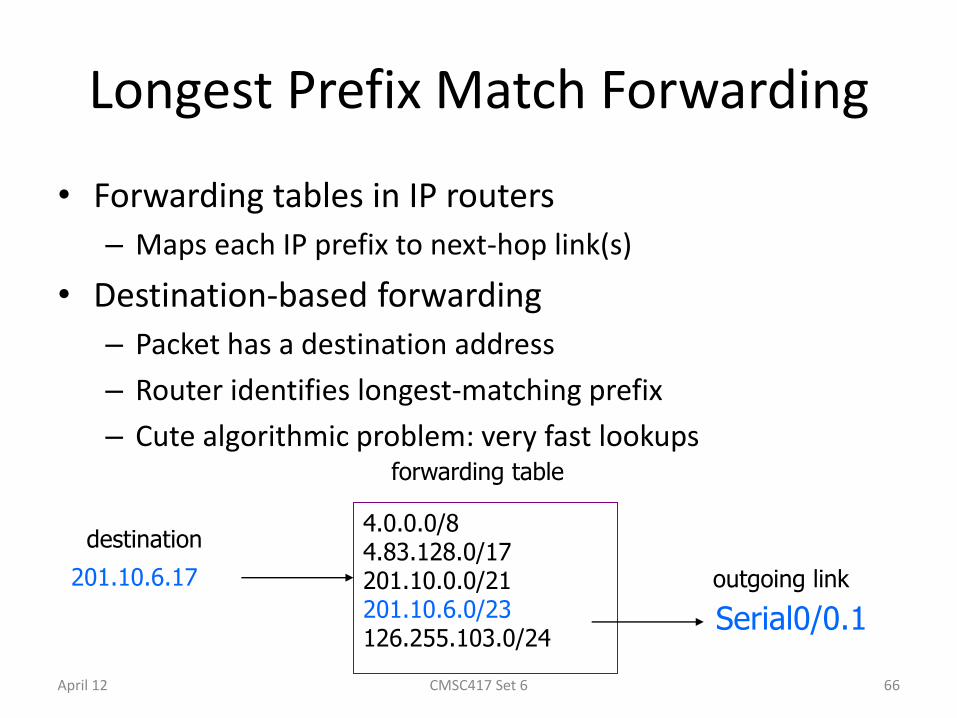
Longest Prefix Match Forwarding
• Forwarding tables in IP routers
– Maps each IP prefix to next-hop link(s)
• Destination-based forwarding
– Packet has a destination address
– Router identifies longest-matching prefix
– Cute algorithmic problem: very fast lookups
66
4.0.0.0/8 4.83.128.0/17 201.10.0.0/21 201.10.6.0/23 126.255.103.0/24
201.10.6.17
destination
forwarding table
Serial0/0.1
outgoing link
April 12 CMSC417 Set 6
Simplest Algorithm is Too Slow
• Scan the forwarding table one entry at a time – See if the destination matches the entry
– If so, check the size of the mask for the prefix
– Keep track of the entry with longest-matching prefix
• Overhead is linear in size of the forwarding table – Today, that means 150,000-200,000 entries!
– And, the router may have just a few nanoseconds
– … before the next packet is arriving
• Need greater efficiency to keep up with line rate – Better algorithms
– Hardware implementations
67 April 12 CMSC417 Set 6
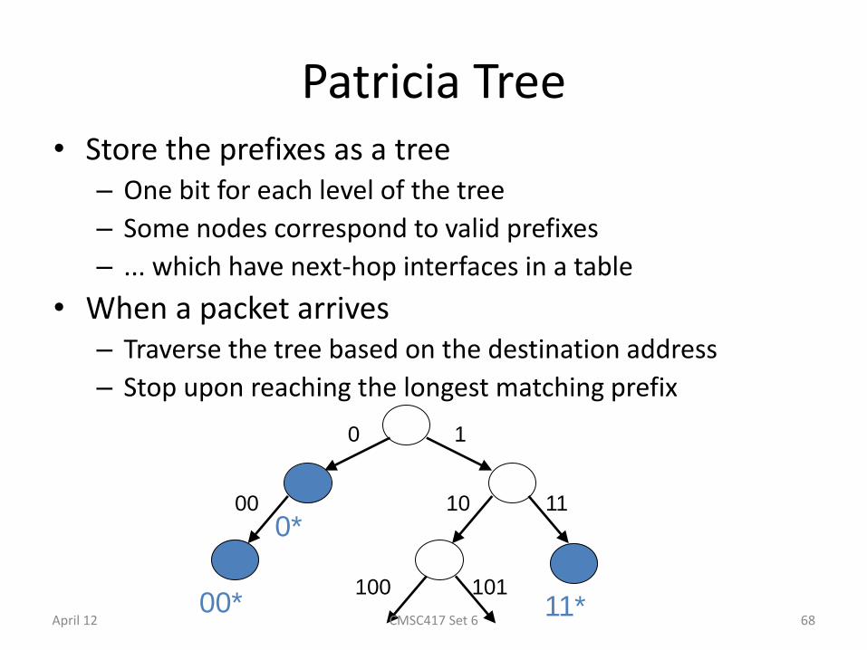
Patricia Tree • Store the prefixes as a tree
– One bit for each level of the tree
– Some nodes correspond to valid prefixes
– ... which have next-hop interfaces in a table
• When a packet arrives – Traverse the tree based on the destination address
– Stop upon reaching the longest matching prefix
68
0 1
00 10 11
100 101 00*
0*
11* April 12 CMSC417 Set 6
Even Faster Lookups
• Patricia tree is faster than linear scan – Proportional to number of bits in the address
• Patricia tree can be made faster – Can make a k-ary tree
• E.g., 4-ary tree with four children (00, 01, 10, and 11)
– Faster lookup, though requires more space
• Can use special hardware – Content Addressable Memories (CAMs) – Allows look-ups on a key rather than flat address
• Huge innovations in the mid-to-late 1990s – After CIDR was introduced (in 1994) – … and longest-prefix match was a major bottleneck
69 April 12 CMSC417 Set 6
Where do Forwarding Tables Come From?
• Routers have forwarding tables – Map prefix to outgoing link(s)
• Entries can be statically configured – E.g., “map 12.34.158.0/24 to Serial0/0.1”
• But, this doesn’t adapt – To failures
– To new equipment
– To the need to balance load
– …
• That is where other technologies come in… – Routing protocols, DHCP, and ARP (later in course)
70 April 12 CMSC417 Set 6
What End Hosts Sending to Others?
• End host with single network interface – PC with an Ethernet link – Laptop with a wireless link
• Don’t need to run a routing protocol – Packets to the host itself (e.g., 1.2.3.4/32)
• Delivered locally
– Packets to other hosts on the LAN (e.g., 1.2.3.0/24) • Sent out the interface
– Packets to external hosts (e.g., 0.0.0.0/0) • Sent out interface to local gateway
• How this information is learned – Static setting of address, subnet mask, and gateway – Dynamic Host Configuration Protocol (DHCP)
71 April 12 CMSC417 Set 6

What About Reaching the End Hosts?
• How does the last router reach the destination?
• Each interface has a persistent, global identifier – MAC (Media Access Control) address – Burned in to the adaptors Read-Only Memory (ROM) – Flat address structure (i.e., no hierarchy)
• Constructing an address resolution table – Mapping MAC address to/from IP address – Address Resolution Protocol (ARP)
72
host host host
LAN
...
router
1.2.3.4 1.2.3.7 1.2.3.156
April 12 CMSC417 Set 6

Conclusions
• IP address
– A 32-bit number
– Allocated in prefixes
– Non-uniform hierarchy for scalability and flexibility
• Packet forwarding
– Based on IP prefixes
– Longest-prefix-match forwarding
• We’ll cover some topics later
– Routing protocols, DHCP, and ARP
73 April 12 CMSC417 Set 6
Routing
April 12 74 CMSC417 Set 6

Routing Algorithms • The Optimality Principle
• Shortest Path Routing
• Flooding
• Distance Vector Routing
• Link State Routing
• Hierarchical Routing
• Broadcast Routing
• Multicast Routing
• Routing for Mobile Hosts
• Routing in Ad Hoc Networks April 12 CMSC417 Set 6 75

Routing Algorithms (2)
Conflict between fairness and optimality.
April 12 CMSC417 Set 6 76
What is Routing?
• A famous quotation from RFC 791 “A name indicates what we seek.
An address indicates where it is. A route indicates how we get there.” -- Jon Postel
April 12 77 CMSC417 Set 6
Routing vs. Forwarding • Routing: control plane
– Computing paths the packets will follow
– Routers talking amongst themselves
– Individual router creating a forwarding table
• Forwarding: data plane
– Directing a data packet to an outgoing link
– Individual router using a forwarding table
April 12 78 CMSC417 Set 6
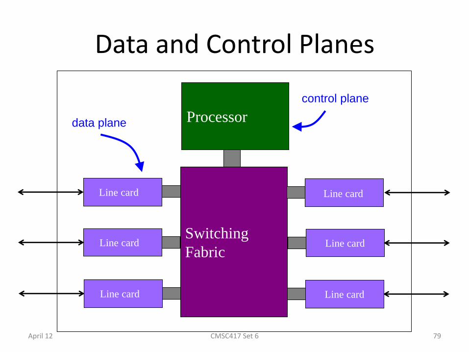
Data and Control Planes
Switching
Fabric
Processor
Line card
Line card
Line card
Line card
Line card
Line card
data plane
control plane
April 12 79 CMSC417 Set 6
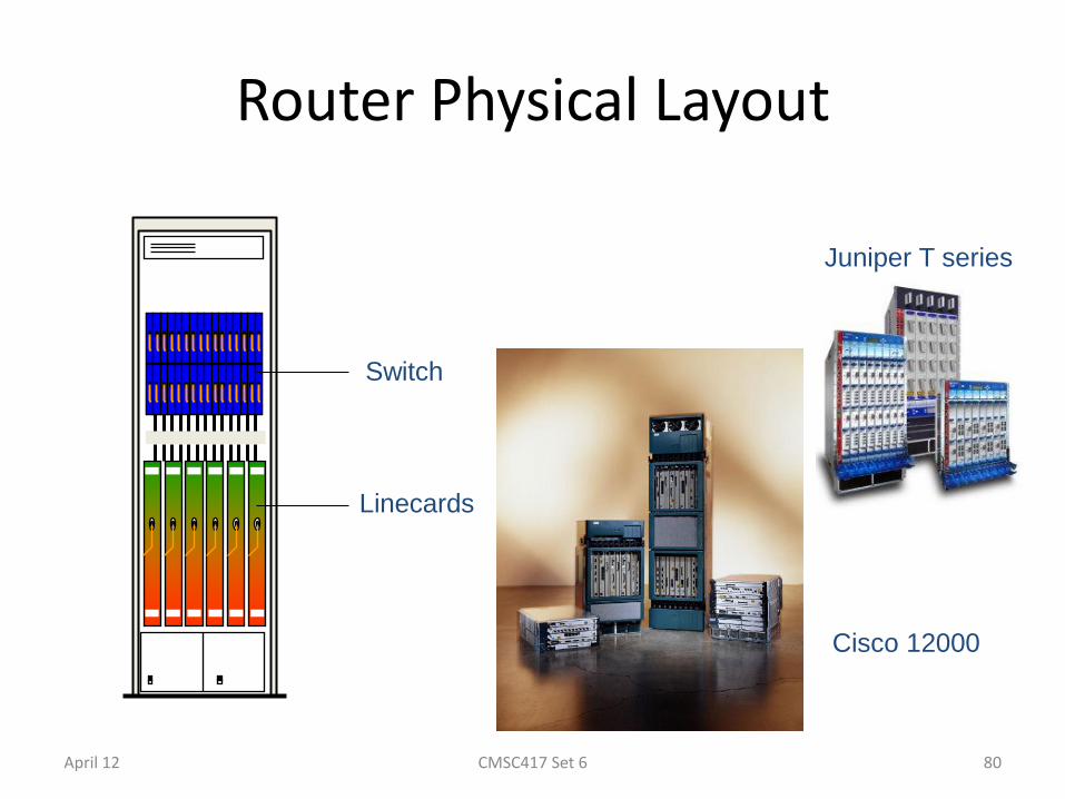
Router Physical Layout
Juniper T series
Cisco 12000
Switch
Linecards
April 12 80 CMSC417 Set 6
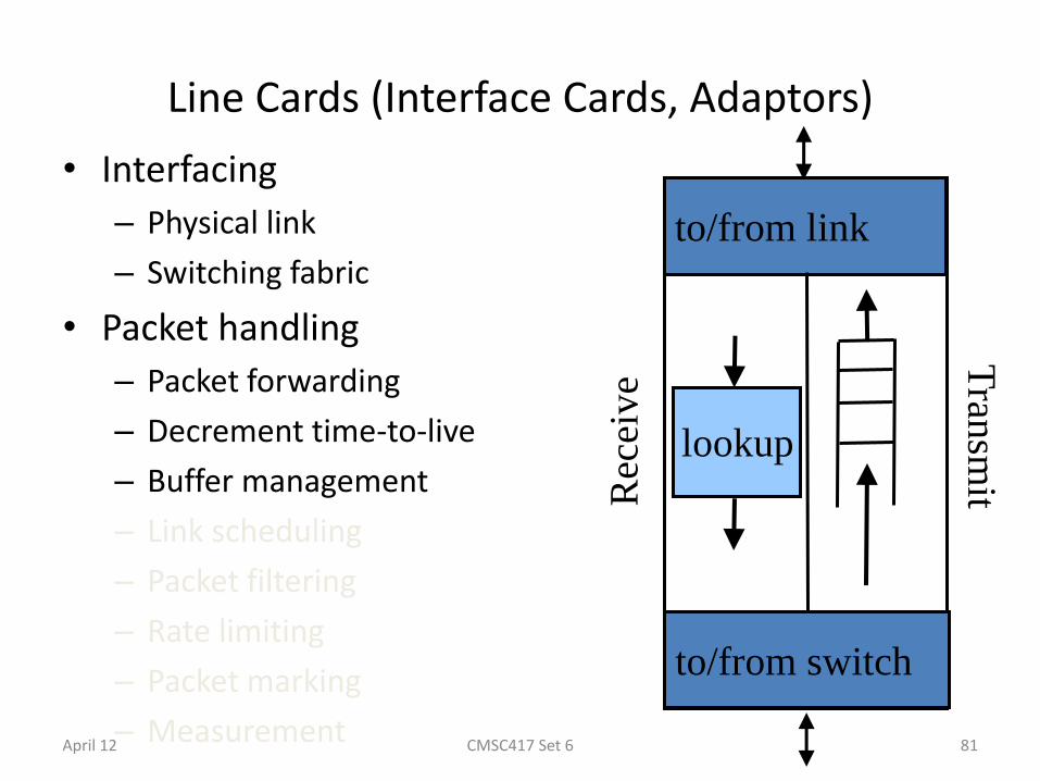
Line Cards (Interface Cards, Adaptors)
• Interfacing
– Physical link
– Switching fabric
• Packet handling
– Packet forwarding
– Decrement time-to-live
– Buffer management
– Link scheduling
– Packet filtering
– Rate limiting
– Packet marking
– Measurement
to/from link
to/from switch
lookup
Rec
eiv
e
Tran
smit
April 12 81 CMSC417 Set 6
Switching Fabric
• Deliver packet inside the router – From incoming interface to outgoing interface
– A small network in and of itself
• Must operate very quickly – Multiple packets going to same outgoing interface
– Switch scheduling to match inputs to outputs
• Implementation techniques – Bus, crossbar, interconnection network, …
– Running at a faster speed (e.g., 2X) than links
– Dividing variable-length packets into fixed-size cells
April 12 82 CMSC417 Set 6
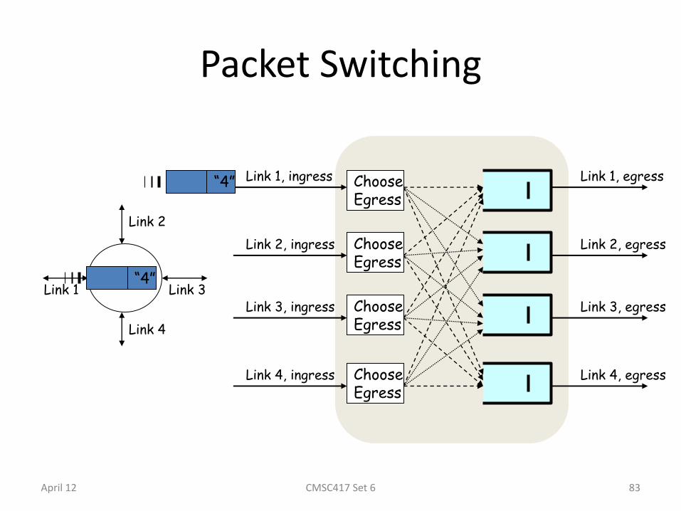
Packet Switching
R1 Link 1
Link 2
Link 3
Link 4
Link 1, ingress Link 1, egress
Link 2, ingress Link 2, egress
Link 3, ingress Link 3, egress
Link 4, ingress Link 4, egress
Choose Egress
Choose Egress
Choose Egress
Choose Egress
“4”
“4”
April 12 83 CMSC417 Set 6
Router Processor
• So-called “Loopback” interface – IP address of the CPU on the router
• Interface to network administrators – Command-line interface for configuration – Transmission of measurement statistics
• Handling of special data packets – Packets with IP options enabled – Packets with expired Time-To-Live field
• Control-plane software – Implementation of the routing protocols – Creation of forwarding table for the line cards
April 12 84 CMSC417 Set 6
Where do Forwarding Tables Come From?
• Routers have forwarding tables – Map IP prefix to outgoing link(s)
• Entries can be statically configured – E.g., “map 12.34.158.0/24 to Serial0/0.1”
• But, this doesn’t adapt – To failures
– To new equipment
– To the need to balance load
• That is where routing protocols come in
April 12 85 CMSC417 Set 6
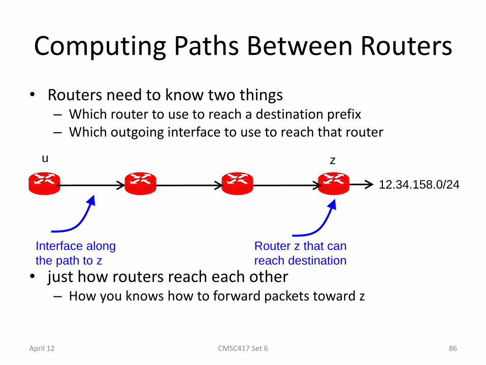
Computing Paths Between Routers
• Routers need to know two things – Which router to use to reach a destination prefix – Which outgoing interface to use to reach that router
• just how routers reach each other – How you knows how to forward packets toward z
12.34.158.0/24
Interface along
the path to z
u z
Router z that can
reach destination
April 12 86 CMSC417 Set 6
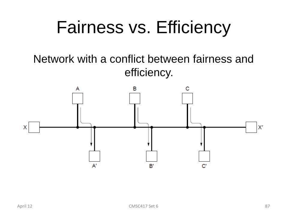
Fairness vs. Efficiency
Network with a conflict between fairness and
efficiency.
April 12 CMSC417 Set 6 87
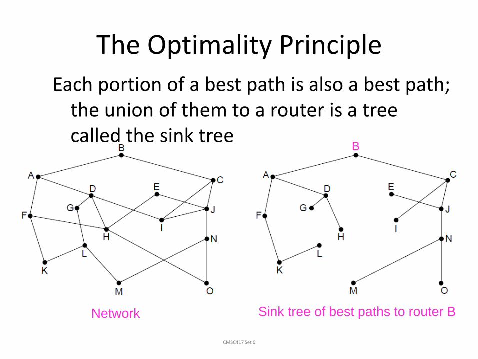
The Optimality Principle
CMSC417 Set 6
Each portion of a best path is also a best path; the union of them to a router is a tree called the sink tree
– Best means fewest hops in the example
Network Sink tree of best paths to router B
B

Computing the Shortest Paths
(assuming you already know the topology)
April 12 89 CMSC417 Set 6
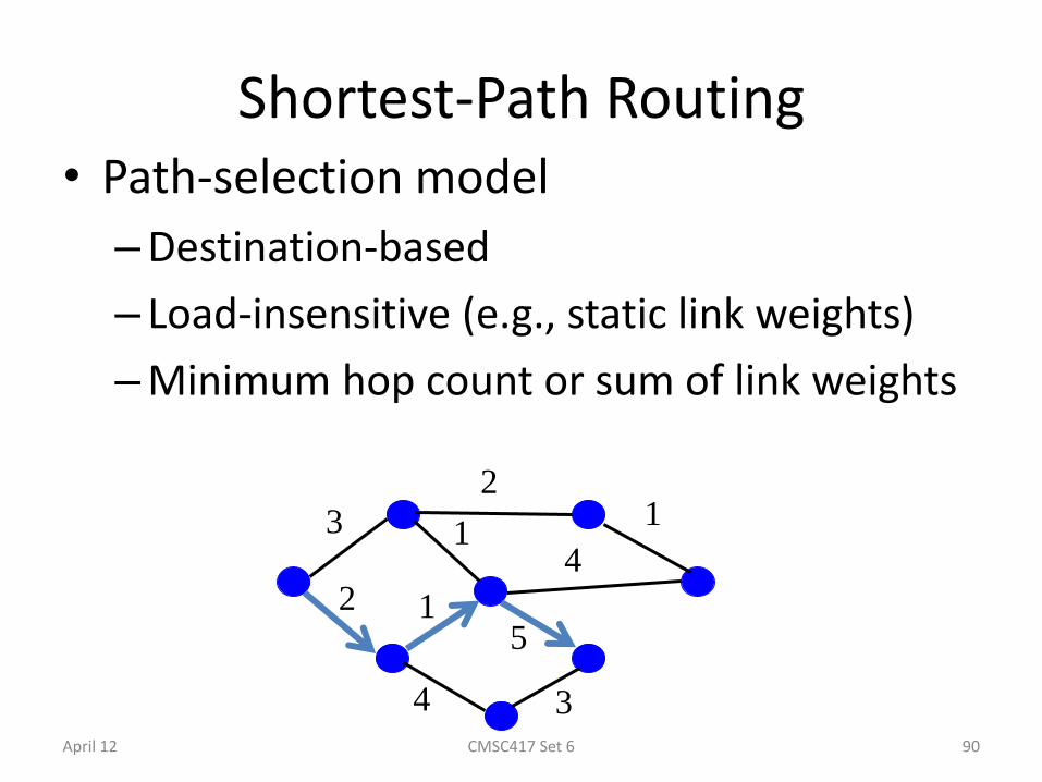
Shortest-Path Routing • Path-selection model
– Destination-based
– Load-insensitive (e.g., static link weights)
– Minimum hop count or sum of link weights
3
2
2
1
1
4
1
4
5
3 April 12 90 CMSC417 Set 6
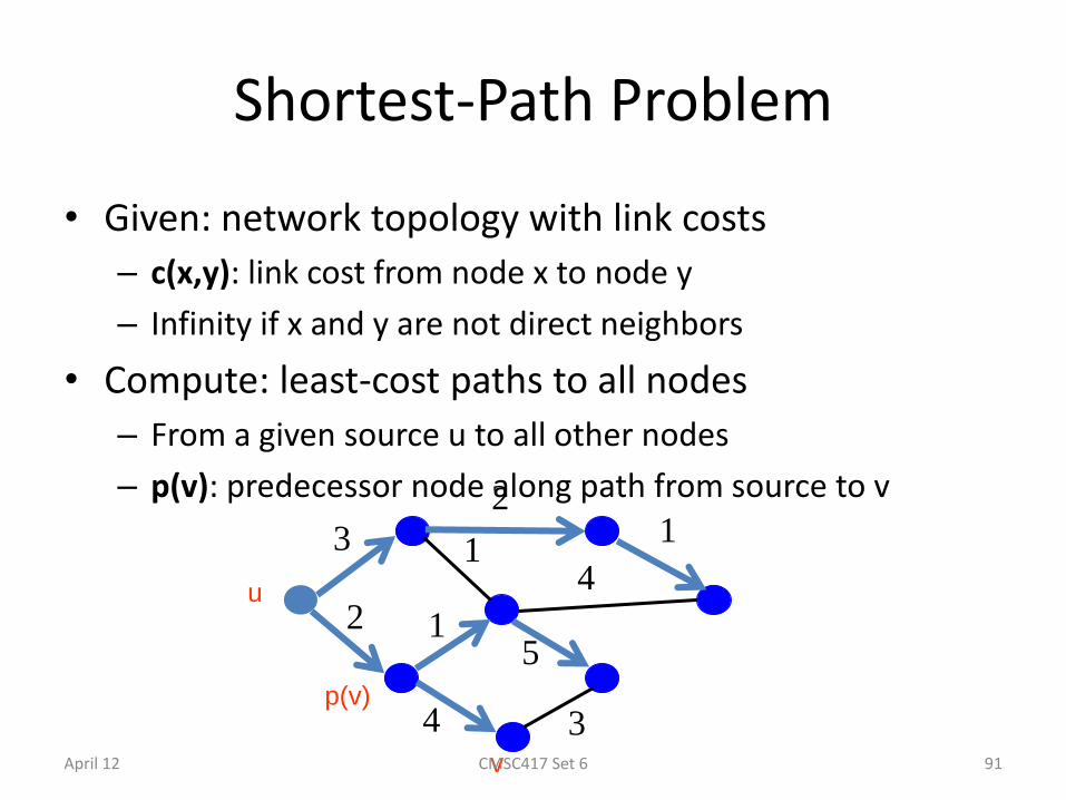
Shortest-Path Problem
• Given: network topology with link costs
– c(x,y): link cost from node x to node y
– Infinity if x and y are not direct neighbors
• Compute: least-cost paths to all nodes
– From a given source u to all other nodes
– p(v): predecessor node along path from source to v
3
2
2
1
1
4
1
4
5
3
u
v
p(v)
April 12 91 CMSC417 Set 6
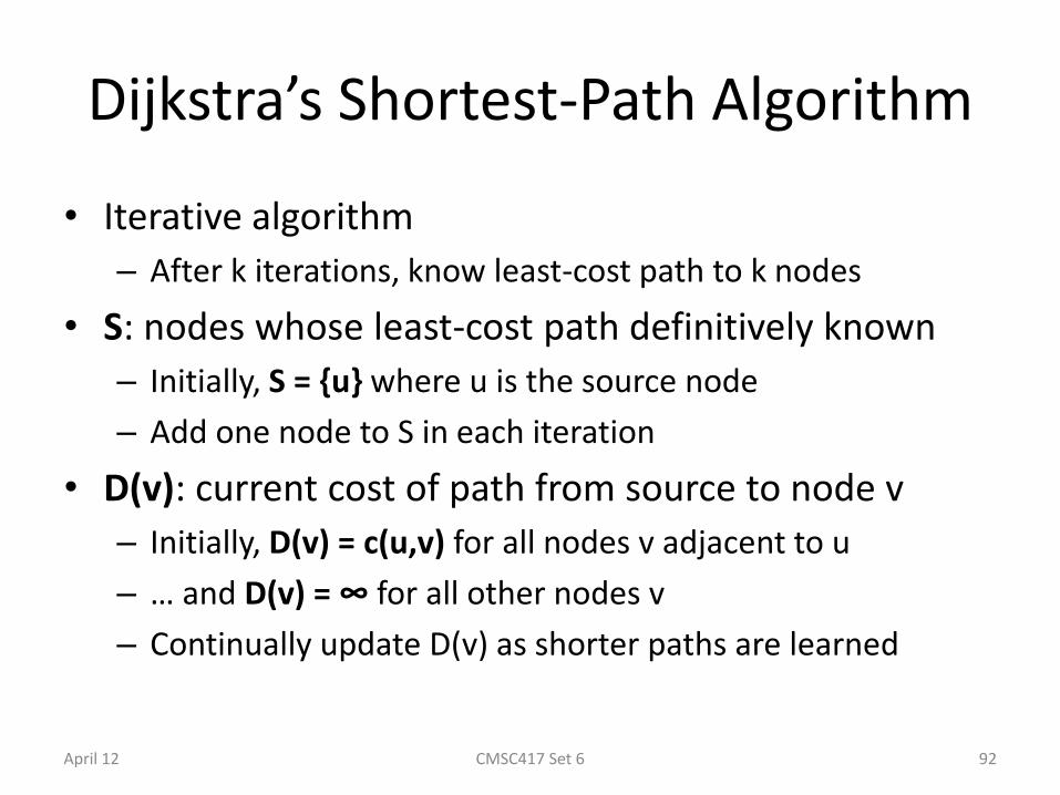
Dijkstra’s Shortest-Path Algorithm
• Iterative algorithm
– After k iterations, know least-cost path to k nodes
• S: nodes whose least-cost path definitively known
– Initially, S = {u} where u is the source node
– Add one node to S in each iteration
• D(v): current cost of path from source to node v
– Initially, D(v) = c(u,v) for all nodes v adjacent to u
– … and D(v) = ∞ for all other nodes v
– Continually update D(v) as shorter paths are learned
April 12 92 CMSC417 Set 6
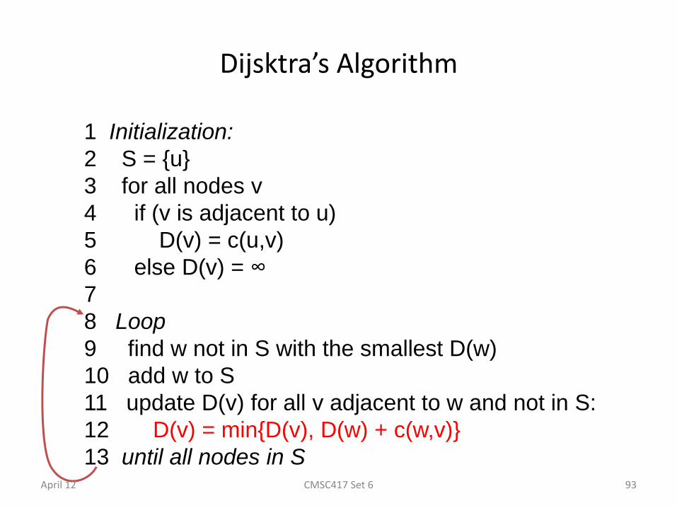
Dijsktra’s Algorithm
1 Initialization:
2 S = {u}
3 for all nodes v
4 if (v is adjacent to u)
5 D(v) = c(u,v)
6 else D(v) = ∞
7
8 Loop
9 find w not in S with the smallest D(w)
10 add w to S
11 update D(v) for all v adjacent to w and not in S:
12 D(v) = min{D(v), D(w) + c(w,v)}
13 until all nodes in S April 12 93 CMSC417 Set 6

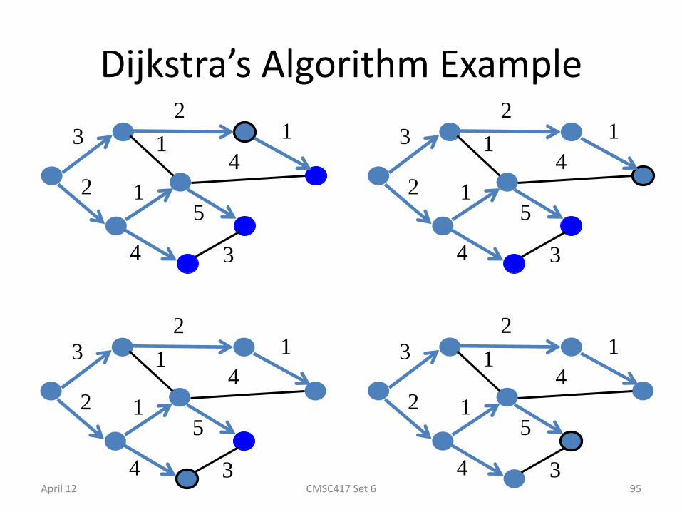
Dijkstra’s Algorithm Example
3
2
2
1
1
4
1
4
5
3
3
2
2
1
1
4
1
4
5
3
3
2
2
1
1
4
1
4
5
3
3
2
2
1
1
4
1
4
5
3 April 12 94 CMSC417 Set 6
Dijkstra’s Algorithm Example
3
2
2
1
1
4
1
4
5
3
3
2
2
1
1
4
1
4
5
3
3
2
2
1
1
4
1
4
5
3
3
2
2
1
1
4
1
4
5
3 April 12 95 CMSC417 Set 6
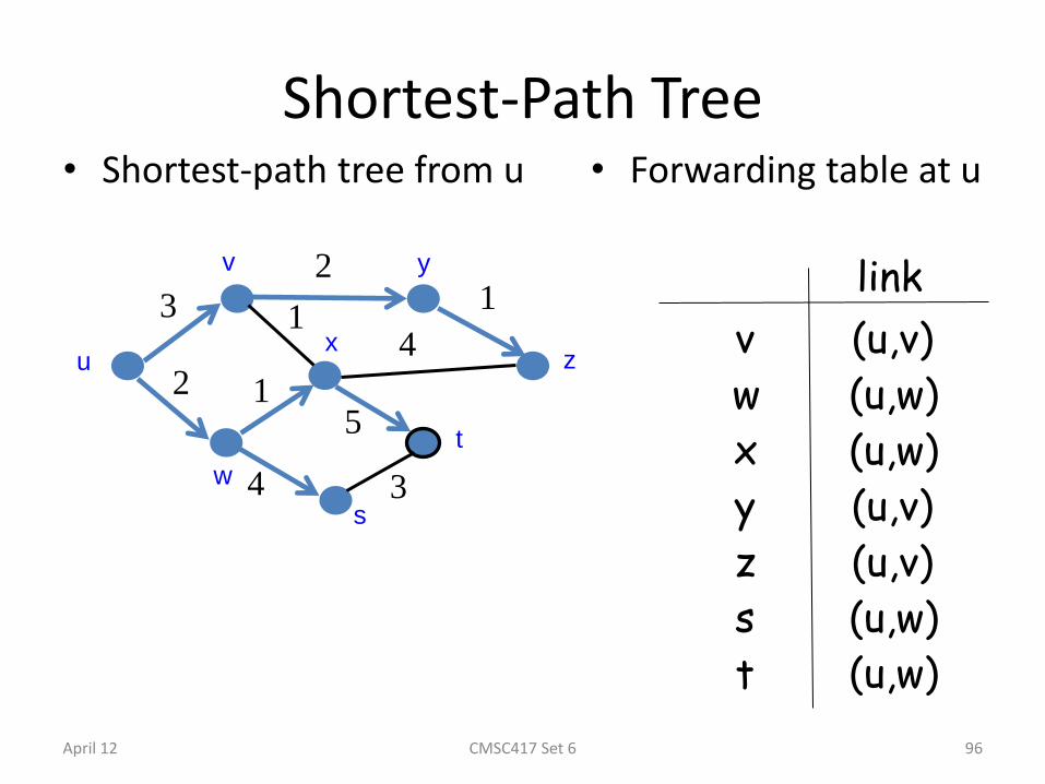
Shortest-Path Tree • Shortest-path tree from u • Forwarding table at u
3
2
2
1
1
4
1
4
5
3
u
v
w
x
y
z
s
t
v (u,v)
w (u,w)
x (u,w)
y (u,v)
z (u,v)
link
s (u,w)
t (u,w)
April 12 96 CMSC417 Set 6

Shortest Path Algorithm (2)
CMSC417 Set 6
A network and first five steps in computing the shortest
paths from A to D. Pink arrows show the sink tree so far. April 12 97
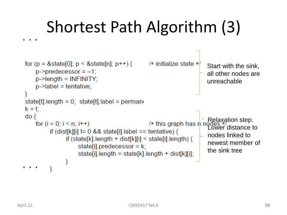
Shortest Path Algorithm (3)
CMSC417 Set 6
. . .
. . .
Start with the sink,
all other nodes are
unreachable
Relaxation step.
Lower distance to
nodes linked to
newest member of
the sink tree
April 12 98

Shortest Path Algorithm (4)
CMSC417 Set 6
. . .
Find the lowest
distance, add it to
the sink tree, and
repeat until done
April 12 99

Shortest path
Dijkstra's algorithm to compute the shortest path through a graph.
5-8 top
April 12 CMSC417 Set 6 100

Shortest path (2)
Dijkstra's algorithm to compute the shortest path through a graph.
5-8
bottom
April 12 CMSC417 Set 6 101
Learning the Topology
(by the routers talking among themselves)
April 12 102 CMSC417 Set 6
Link-State Routing
• Each router keeps track of its incident links – Whether the link is up or down
– The cost on the link
• Each router broadcasts the link state – To give every router a complete view of the graph
• Each router runs Dijkstra’s algorithm – To compute the shortest paths
– … and construct the forwarding table
• Example protocols – Open Shortest Path First (OSPF)
– Intermediate System – Intermediate System (IS-IS)
April 12 103 CMSC417 Set 6
Link State Routing Each router must do the following:
1. Discover its neighbors, learn their network address.
2. Measure the delay or cost to each of its neighbors.
3. Construct a packet telling all it has just learned.
4. Send this packet to all other routers.
5. Compute the shortest path to every other router.
April 12 CMSC417 Set 6 104
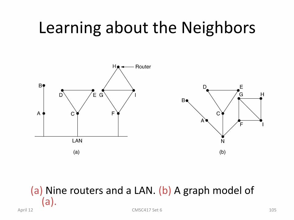
Learning about the Neighbors
(a) Nine routers and a LAN. (b) A graph model of (a).
April 12 CMSC417 Set 6 105
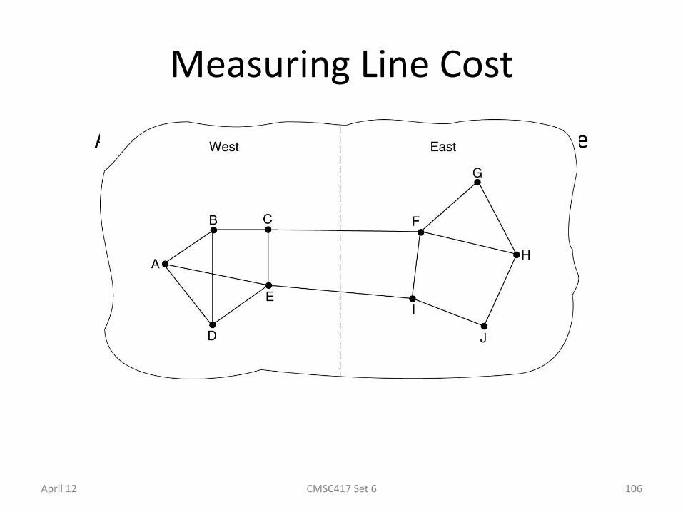
Measuring Line Cost
A subnet in which the East and West parts are connected by two lines.
April 12 CMSC417 Set 6 106

Building Link State Packets
(a) A subnet. (b) The link state packets for this subnet.
April 12 CMSC417 Set 6 107
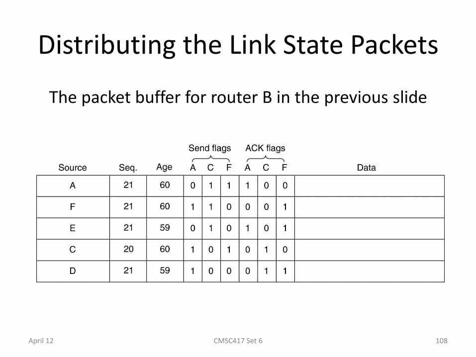
Distributing the Link State Packets
The packet buffer for router B in the previous slide
April 12 CMSC417 Set 6 108
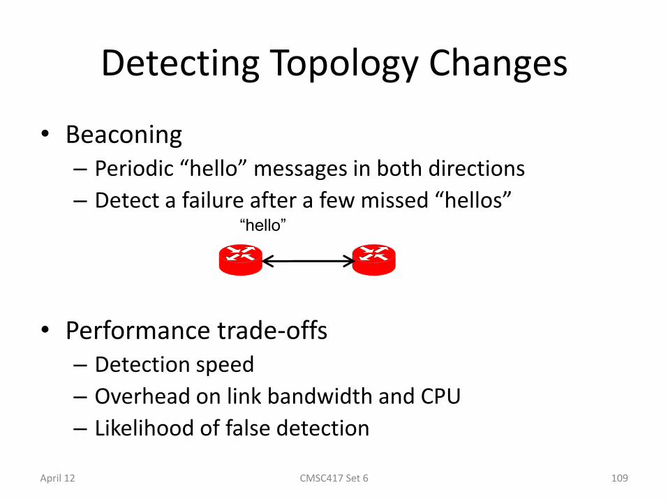
Detecting Topology Changes
• Beaconing – Periodic “hello” messages in both directions
– Detect a failure after a few missed “hellos”
• Performance trade-offs – Detection speed
– Overhead on link bandwidth and CPU
– Likelihood of false detection
“hello”
April 12 109 CMSC417 Set 6
Broadcasting the Link State
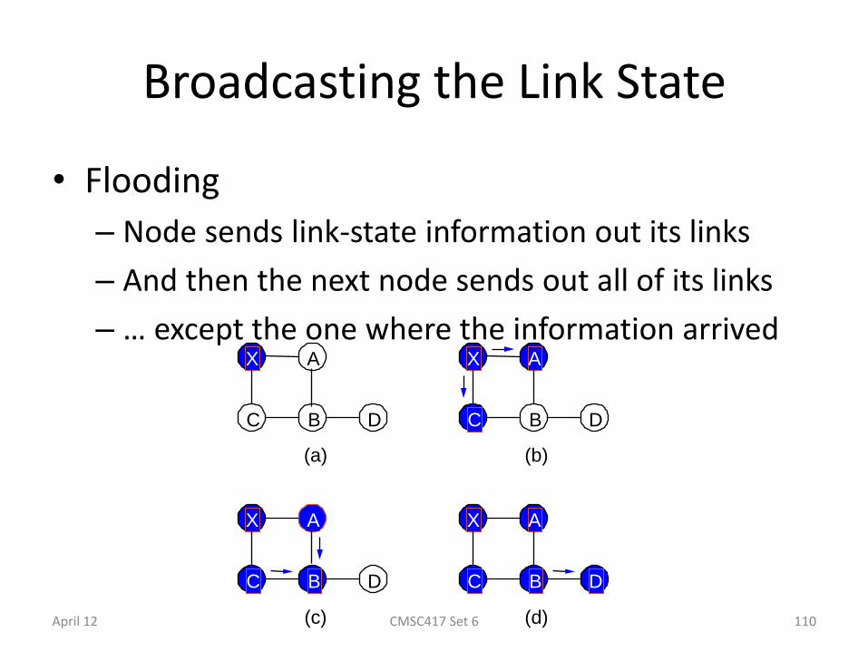
• Flooding
– Node sends link-state information out its links
– And then the next node sends out all of its links
– … except the one where the information arrived X A
C B D
(a)
X A
C B D
(b)
X A
C B D
(c)
X A
C B D
(d) April 12 110 CMSC417 Set 6
Broadcasting the Link State
• Reliable flooding – Ensure all nodes receive link-state information – … and that they use the latest version
• Challenges – Packet loss – Out-of-order arrival
• Solutions – Acknowledgments and retransmissions – Sequence numbers – Time-to-live for each packet
April 12 111 CMSC417 Set 6

When to Initiate Flooding
• Topology change – Link or node failure
– Link or node recovery
• Configuration change – Link cost change
• Periodically – Refresh the link-state information
– Typically (say) 30 minutes
– Corrects for possible corruption of the data
April 12 112 CMSC417 Set 6
When the Routers Disagree
(during transient periods)
April 12 113 CMSC417 Set 6
Convergence
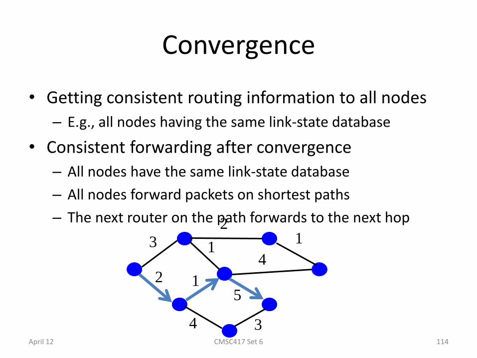
• Getting consistent routing information to all nodes
– E.g., all nodes having the same link-state database
• Consistent forwarding after convergence
– All nodes have the same link-state database
– All nodes forward packets on shortest paths
– The next router on the path forwards to the next hop
3
2
2
1
1
4
1
4
5
3 April 12 114 CMSC417 Set 6

Transient Disruptions
• Detection delay
– A node does not detect a failed link immediately
– … and forwards data packets into a “blackhole”
– Depends on timeout for detecting lost hellos
3
2
2
1
1
4
1
4
5
3
April 12 115 CMSC417 Set 6
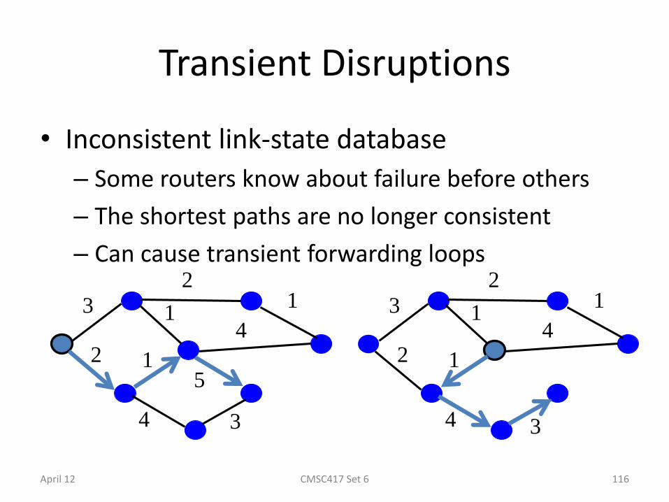
Transient Disruptions
• Inconsistent link-state database
– Some routers know about failure before others
– The shortest paths are no longer consistent
– Can cause transient forwarding loops
3
2
2
1
1
4
1
4
5
3
3
2
2
1
1
4
1
4 3
April 12 116 CMSC417 Set 6
Convergence Delay
• Sources of convergence delay – Detection latency – Flooding of link-state information – Shortest-path computation – Creating the forwarding table
• Performance during convergence period – Lost packets due to blackholes and TTL expiry – Looping packets consuming resources – Out-of-order packets reaching the destination
• Very bad for VoIP, online gaming, and video
April 12 117 CMSC417 Set 6
Reducing Convergence Delay
• Faster detection – Smaller hello timers
– Link-layer technologies that can detect failures
• Faster flooding – Flooding immediately
– Sending link-state packets with high-priority
• Faster computation – Faster processors on the routers
– Incremental Dijkstra’s algorithm
• Faster forwarding-table update – Data structures supporting incremental updates
April 12 118 CMSC417 Set 6
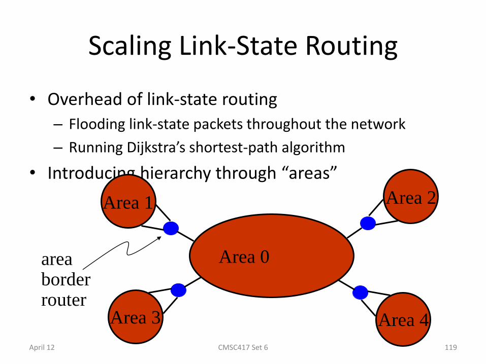
Scaling Link-State Routing
• Overhead of link-state routing
– Flooding link-state packets throughout the network
– Running Dijkstra’s shortest-path algorithm
• Introducing hierarchy through “areas”
Area 0
Area 1 Area 2
Area 3 Area 4
area border router
April 12 119 CMSC417 Set 6

Some Properties
• Routing is a distributed algorithm – React to changes in the topology
– Compute the paths through the network
• Shortest-path link state routing – Flood link weights throughout the network
– Compute shortest paths as a sum of link weights
– Forward packets on next hop in the shortest path
• Convergence process – Changing from one topology to another
– Transient periods of inconsistency across routers
April 12 120 CMSC417 Set 6

Distance Vector Routing
(a) A subnet. (b) Input from A, I, H, K, and the new routing table for J.
April 12 CMSC417 Set 6 121

Distance Vector Algorithm
• c(x,v) = cost for direct link from x to v – Node x maintains costs of direct links c(x,v)
• Dx(y) = estimate of least cost from x to y – Node x maintains distance vector Dx = [Dx(y): y є N ]
• Node x maintains its neighbors’ distance vectors – For each neighbor v, x maintains Dv = [Dv(y): y є N ]
• Each node v periodically sends Dv to its neighbors – And neighbors update their own distance vectors
– Dx(y) ← minv{c(x,v) + Dv(y)} for each node y ∊ N
• Over time, the distance vector Dx converges
April 12 122 CMSC417 Set 6
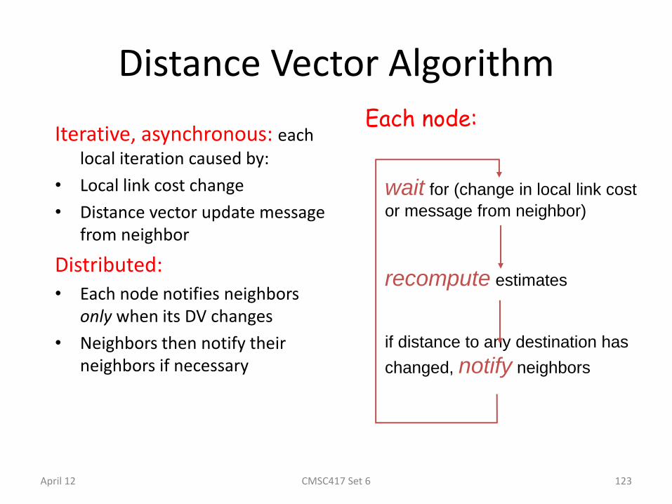
Distance Vector Algorithm
Iterative, asynchronous: each
local iteration caused by:
• Local link cost change
• Distance vector update message from neighbor
Distributed: • Each node notifies neighbors
only when its DV changes
• Neighbors then notify their neighbors if necessary
wait for (change in local link cost
or message from neighbor)
recompute estimates
if distance to any destination has
changed, notify neighbors
Each node:
April 12 123 CMSC417 Set 6
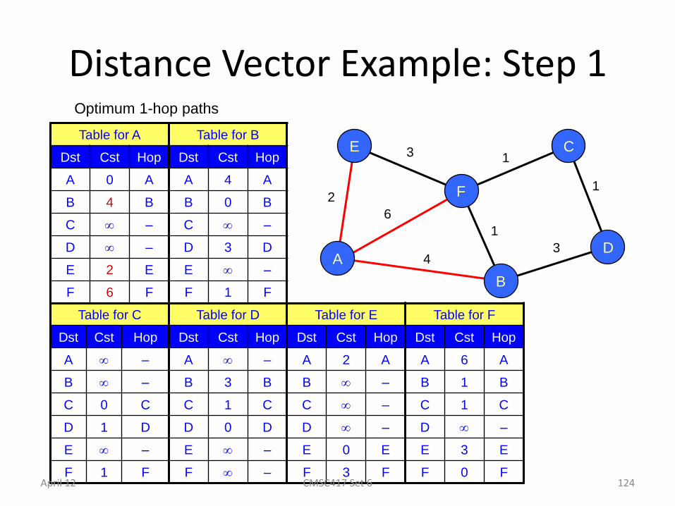
Distance Vector Example: Step 1
A
E
F
C
D
B
2
3
6
4
1
1
1
3
Table for A
Dst Cst Hop
A 0 A
B 4 B
C –
D –
E 2 E
F 6 F
Table for B
Dst Cst Hop
A 4 A
B 0 B
C –
D 3 D
E –
F 1 F
Table for C
Dst Cst Hop
A –
B –
C 0 C
D 1 D
E –
F 1 F
Table for D
Dst Cst Hop
A –
B 3 B
C 1 C
D 0 D
E –
F –
Table for E
Dst Cst Hop
A 2 A
B –
C –
D –
E 0 E
F 3 F
Table for F
Dst Cst Hop
A 6 A
B 1 B
C 1 C
D –
E 3 E
F 0 F
Optimum 1-hop paths
April 12 124 CMSC417 Set 6
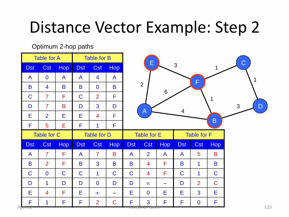
Distance Vector Example: Step 2
Table for A
Dst Cst Hop
A 0 A
B 4 B
C 7 F
D 7 B
E 2 E
F 5 E
Table for B
Dst Cst Hop
A 4 A
B 0 B
C 2 F
D 3 D
E 4 F
F 1 F
Table for C
Dst Cst Hop
A 7 F
B 2 F
C 0 C
D 1 D
E 4 F
F 1 F
Table for D
Dst Cst Hop
A 7 B
B 3 B
C 1 C
D 0 D
E –
F 2 C
Table for E
Dst Cst Hop
A 2 A
B 4 F
C 4 F
D –
E 0 E
F 3 F
Table for F
Dst Cst Hop
A 5 B
B 1 B
C 1 C
D 2 C
E 3 E
F 0 F
Optimum 2-hop paths
A
E
F
C
D
B
2
3
6
4
1
1
1
3
April 12 125 CMSC417 Set 6
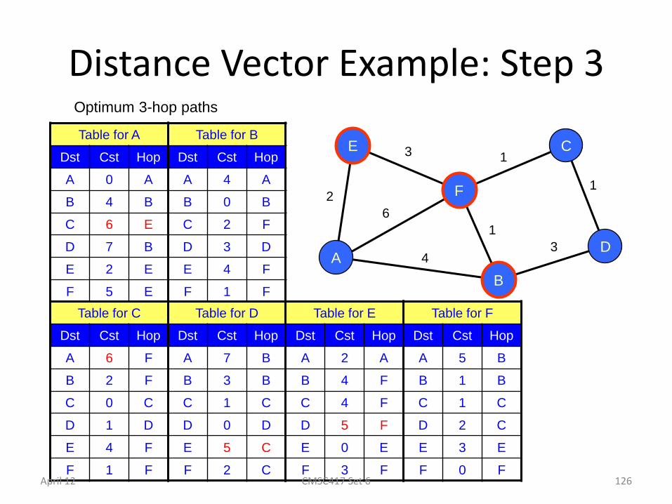
Distance Vector Example: Step 3
Table for A
Dst Cst Hop
A 0 A
B 4 B
C 6 E
D 7 B
E 2 E
F 5 E
Table for B
Dst Cst Hop
A 4 A
B 0 B
C 2 F
D 3 D
E 4 F
F 1 F
Table for C
Dst Cst Hop
A 6 F
B 2 F
C 0 C
D 1 D
E 4 F
F 1 F
Table for D
Dst Cst Hop
A 7 B
B 3 B
C 1 C
D 0 D
E 5 C
F 2 C
Table for E
Dst Cst Hop
A 2 A
B 4 F
C 4 F
D 5 F
E 0 E
F 3 F
Table for F
Dst Cst Hop
A 5 B
B 1 B
C 1 C
D 2 C
E 3 E
F 0 F
Optimum 3-hop paths
A
E
F
C
D
B
2
3
6
4
1
1
1
3
April 12 126 CMSC417 Set 6
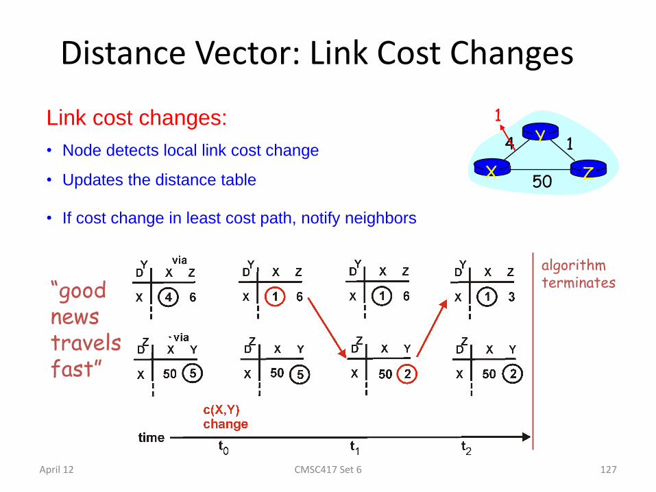
Distance Vector: Link Cost Changes
Link cost changes:
• Node detects local link cost change
• Updates the distance table
• If cost change in least cost path, notify neighbors
X Z
1 4
50
Y 1
algorithm terminates “good
news travels fast”
April 12 127 CMSC417 Set 6
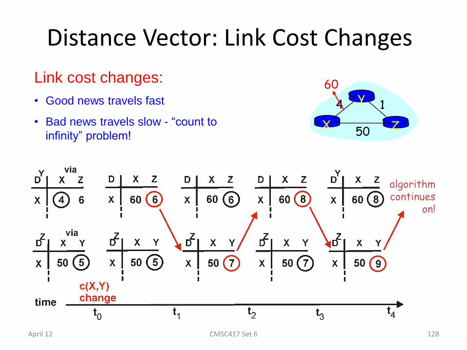
Distance Vector: Link Cost Changes
Link cost changes:
• Good news travels fast
• Bad news travels slow - “count to
infinity” problem! X Z
1 4
50
Y 60
algorithm continues
on!
April 12 128 CMSC417 Set 6
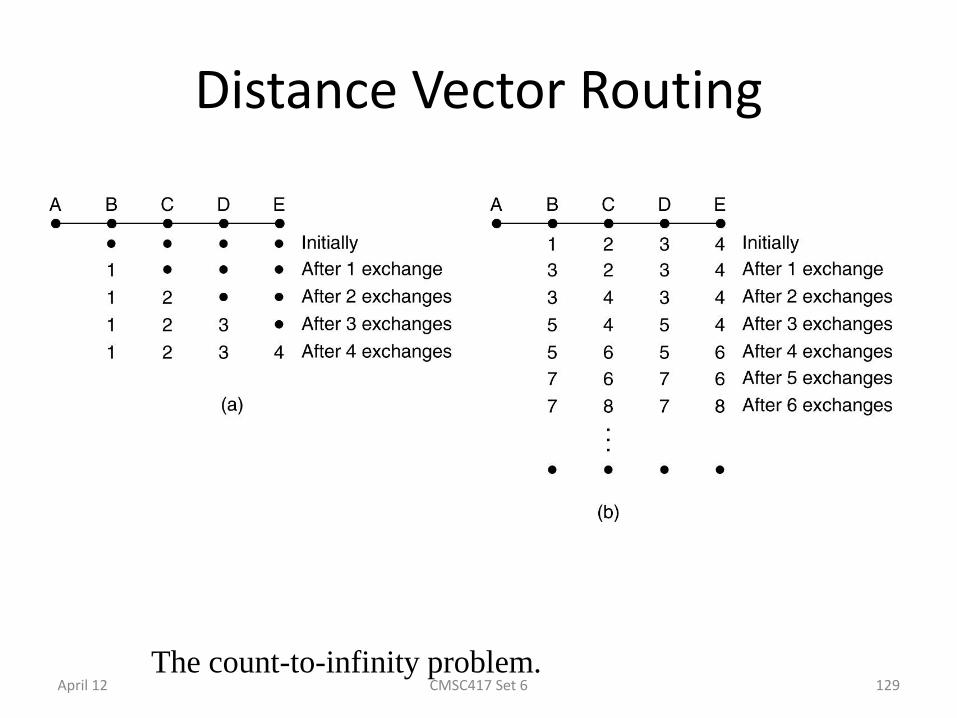
Distance Vector Routing
The count-to-infinity problem. April 12 CMSC417 Set 6 129
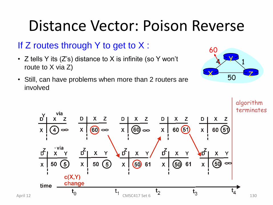
Distance Vector: Poison Reverse If Z routes through Y to get to X :
• Z tells Y its (Z’s) distance to X is infinite (so Y won’t
route to X via Z)
• Still, can have problems when more than 2 routers are
involved
X Z
1 4
50
Y 60
algorithm terminates
April 12 130 CMSC417 Set 6
Routing Information Protocol (RIP)
• Distance vector protocol – Nodes send distance vectors every 30 seconds
– … or, when an update causes a change in routing
• Link costs in RIP – All links have cost 1
– Valid distances of 1 through 15
– … with 16 representing infinity
– Small “infinity” smaller “counting to infinity” problem
• RIP is limited to fairly small networks – E.g., used in some campus networks
April 12 131 CMSC417 Set 6

Comparison of LS and DV Routing Message complexity • LS: with n nodes, E links, O(nE)
messages sent
• DV: exchange between neighbors only
Speed of Convergence • LS: relatively fast
• DV: convergence time varies
– May be routing loops
– Count-to-infinity problem
Robustness: what happens if router malfunctions?
LS: – Node can advertise incorrect
link cost
– Each node computes only its own table
DV: – DV node can advertise
incorrect path cost
– Each node’s table used by others (error propagates)
April 12 132 CMSC417 Set 6
Similarities of LS and DV Routing
• Shortest-path routing – Metric-based, using link weights
– Routers share a common view of how good a path is
• As such, commonly used inside an organization – RIP and OSPF are mostly used as intradomain protocols
– E.g., Princeton uses RIP, and AT&T uses OSPF
• But the Internet is a “network of networks” – How to stitch the many networks together?
– When networks may not have common goals
– … and may not want to share information
April 12 133 CMSC417 Set 6

Hierarchical Routing
Hierarchical routing.
April 12 CMSC417 Set 6 134
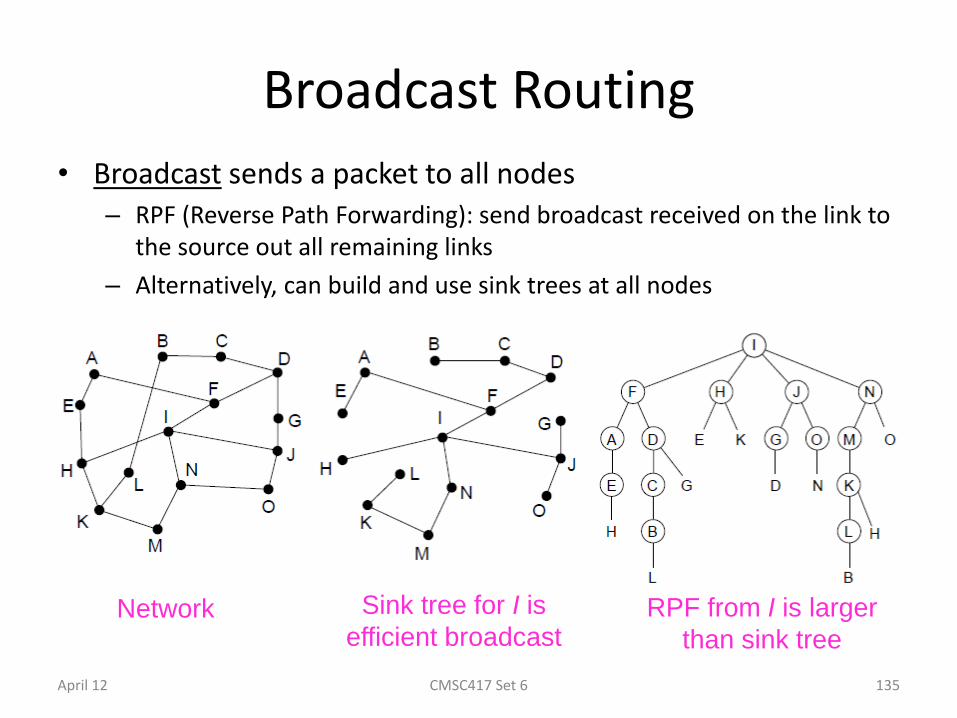
Broadcast Routing
• Broadcast sends a packet to all nodes – RPF (Reverse Path Forwarding): send broadcast received on the link to
the source out all remaining links
– Alternatively, can build and use sink trees at all nodes
CMSC417 Set 6
Network Sink tree for I is
efficient broadcast RPF from I is larger
than sink tree
April 12 135

Multicast Routing (1) – Dense Case • Multicast sends to a subset of the nodes called a group
– Uses a different tree for each group and source
CMSC417 Set 6
Network with groups 1 & 2 Spanning tree from source S
S
S S
Multicast tree from S to group 1 Multicast tree from S to group 2
April 12 136

Multicast Routing (2) – Sparse Case
• CBT (Core-Based Tree) uses a single tree to multicast
– Tree is the sink tree from core node to group members
– Multicast heads to the core until it reaches the CBT
• p 1.
CMSC417 Set 6
Sink tree from core to group 1 Multicast is send to the core then
down when it reaches the sink tree
April 12 137
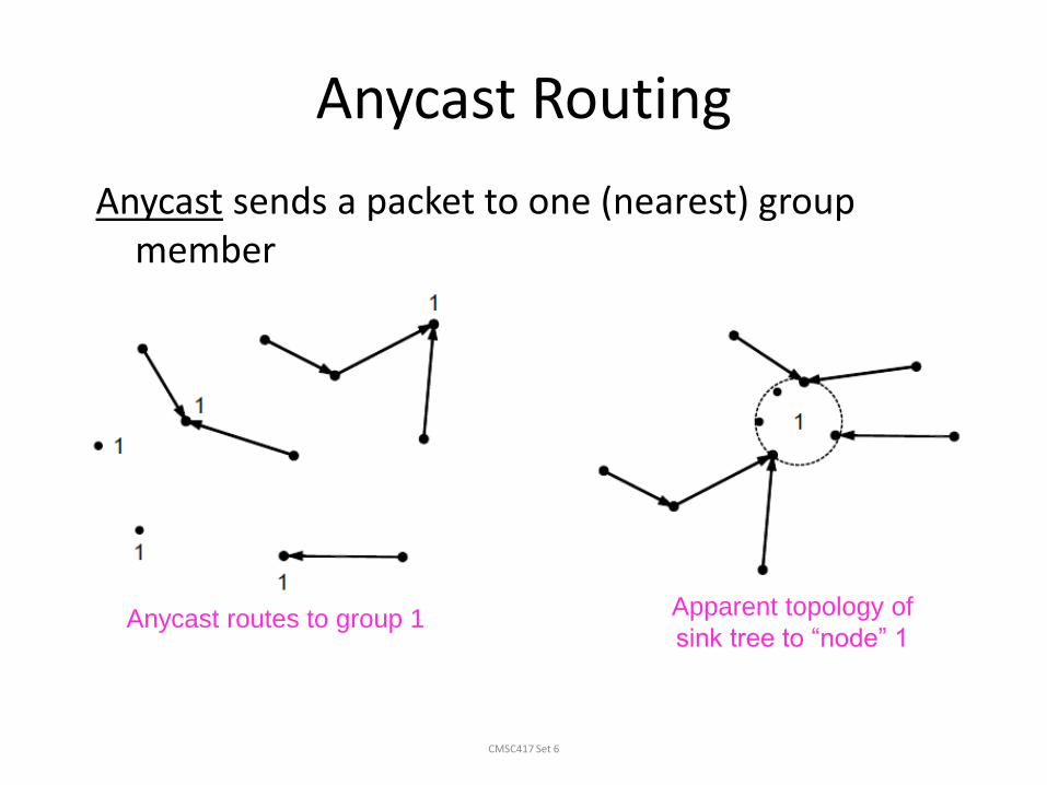
Anycast Routing
CMSC417 Set 6
Anycast sends a packet to one (nearest) group member
– Falls out of regular routing with a node in many places
Anycast routes to group 1 Apparent topology of
sink tree to “node” 1

Routing for Mobile Hosts
A WAN to which LANs, MANs, and wireless cells are attached.
April 12 CMSC417 Set 6 139
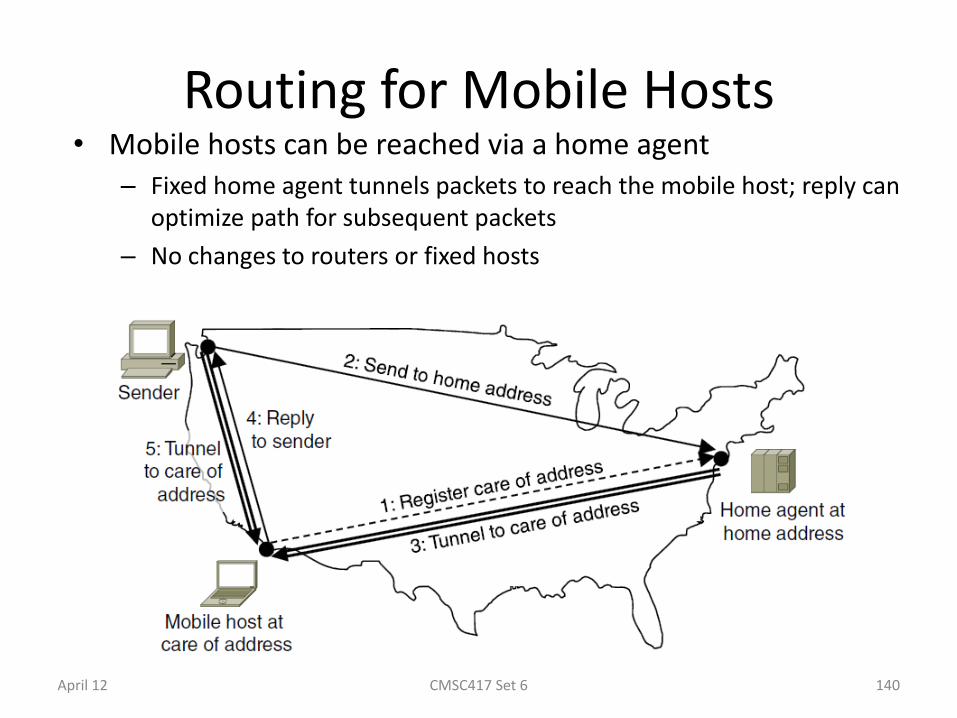
Routing for Mobile Hosts • Mobile hosts can be reached via a home agent
– Fixed home agent tunnels packets to reach the mobile host; reply can optimize path for subsequent packets
– No changes to routers or fixed hosts
CMSC417 Set 6 April 12 140
Routing in Ad Hoc Networks
Possibilities when the routers are mobile:
1.Military vehicles on battlefield.
– No infrastructure.
2.A fleet of ships at sea. – All moving all the time
3.Emergency works at earthquake . – The infrastructure destroyed.
4. A gathering of people with notebook computers.
– In an area lacking 802.11.
April 12 CMSC417 Set 6 141

Route Discovery
• (a) Range of A's broadcast.
• (b) After B and D have received A's broadcast.
• (c) After C, F, and G have received A's broadcast.
• (d) After E, H, and I have received A's broadcast.
Shaded nodes are new recipients. Arrows show possible reverse routes. April 12 CMSC417 Set 6 142
Route Discovery (2)
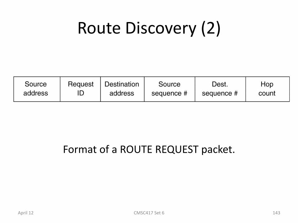
Format of a ROUTE REQUEST packet.
April 12 CMSC417 Set 6 143
Route Discovery (3)
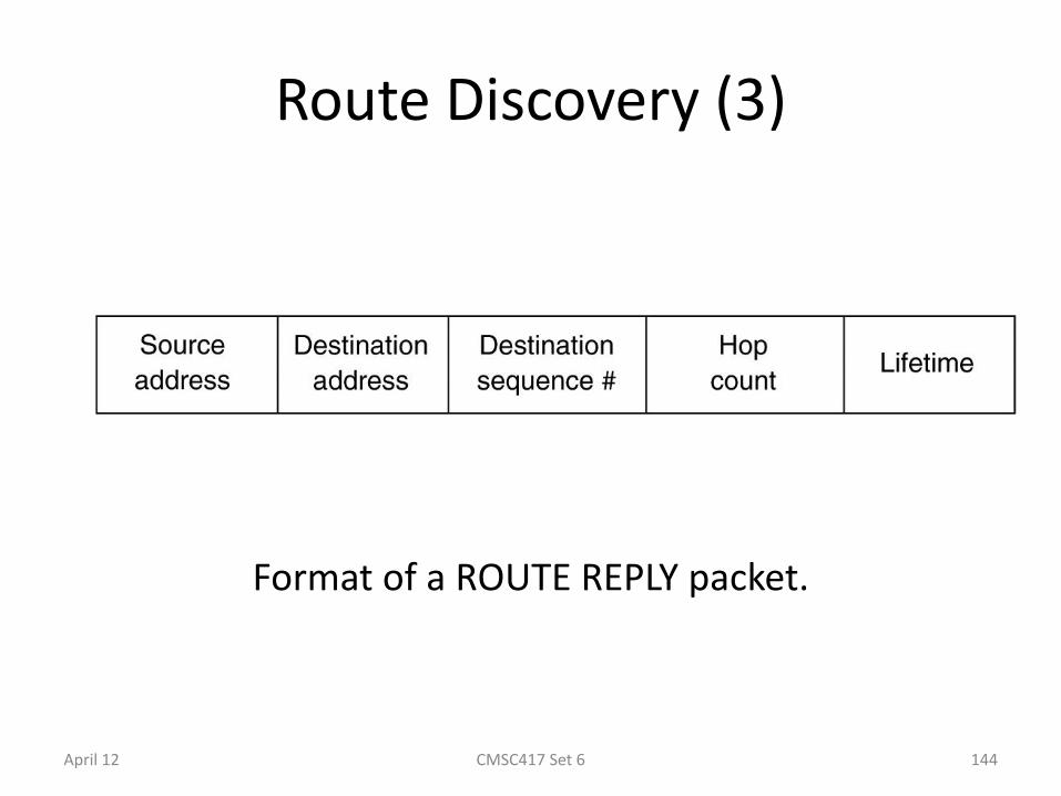
Format of a ROUTE REPLY packet.
April 12 CMSC417 Set 6 144
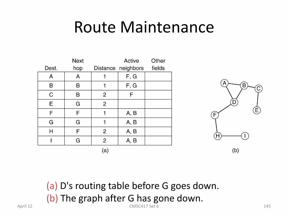
Route Maintenance
(a) D's routing table before G goes down. (b) The graph after G has gone down.
April 12 CMSC417 Set 6 145

Node Lookup in Peer-to-Peer Networks
(a) A set of 32 node identifiers arranged in a circle. The shaded ones correspond to actual machines. The arcs show the fingers from nodes 1, 4, and 12. The labels on the arcs are the table indices.
(b) Examples of the finger tables. April 12 CMSC417 Set 6 146
Congestion Control Algorithms
• General Principles of Congestion Control
• Congestion Prevention Policies
• Congestion Control in Virtual-Circuit Subnets
• Congestion Control in Datagram Subnets
• Load Shedding
• Jitter Control
April 12 CMSC417 Set 6 147
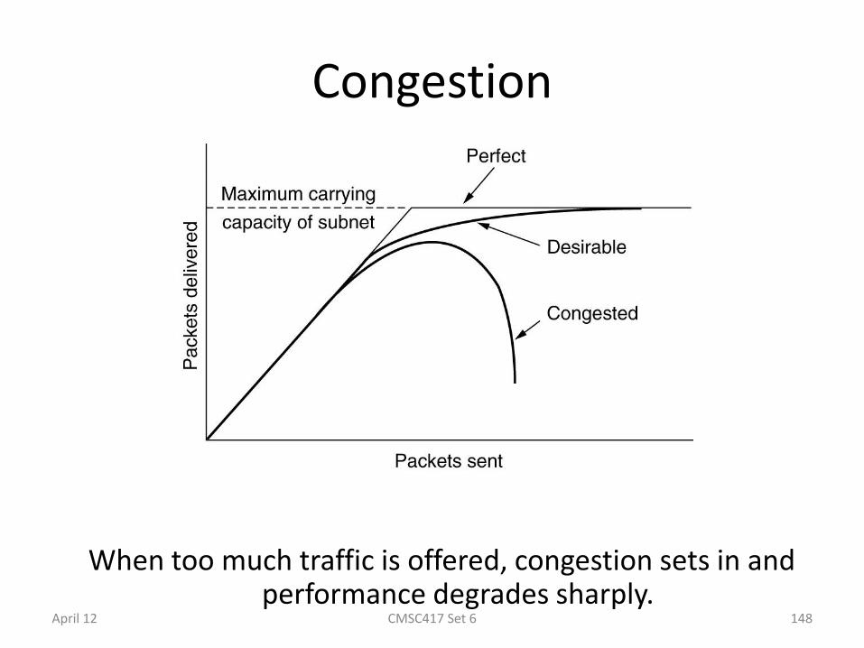
Congestion
When too much traffic is offered, congestion sets in and performance degrades sharply.
April 12 CMSC417 Set 6 148
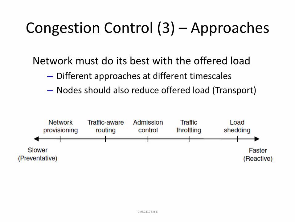
Congestion Control (3) – Approaches
CMSC417 Set 6
Network must do its best with the offered load
– Different approaches at different timescales
– Nodes should also reduce offered load (Transport)

Traffic-Aware Routing
CMSC417 Set 6
Choose routes depending on traffic, not just topology – E.g., use EI for West-to-East traffic if CF is loaded
– But take care to avoid oscillations
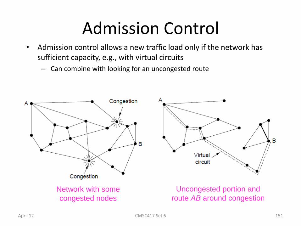
Admission Control • Admission control allows a new traffic load only if the network has
sufficient capacity, e.g., with virtual circuits
– Can combine with looking for an uncongested route
CMSC417 Set 6
Network with some
congested nodes
Uncongested portion and
route AB around congestion
April 12 151
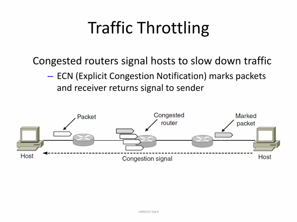
Traffic Throttling
CMSC417 Set 6
Congested routers signal hosts to slow down traffic
– ECN (Explicit Congestion Notification) marks packets and receiver returns signal to sender
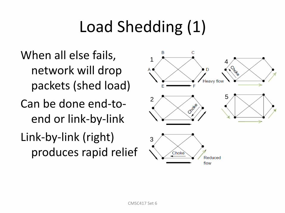
Load Shedding (1)
CMSC417 Set 6
When all else fails, network will drop packets (shed load)
Can be done end-to-end or link-by-link
Link-by-link (right) produces rapid relief
1
3
2
4
5
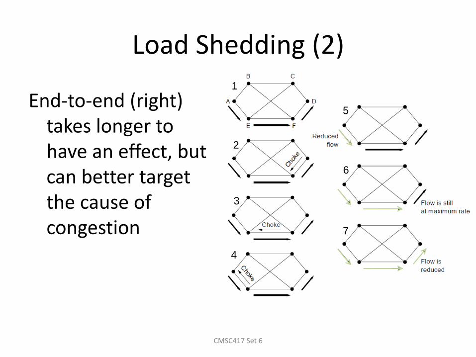
Load Shedding (2)
CMSC417 Set 6
End-to-end (right) takes longer to have an effect, but can better target the cause of congestion
1
3
2
7
5
6
4

General Principles of Congestion Control
1.Monitor the system .
– detect when and where congestion occurs.
2.Pass information to where action can be taken.
3.Adjust system operation to correct the problem.
April 12 CMSC417 Set 6 155
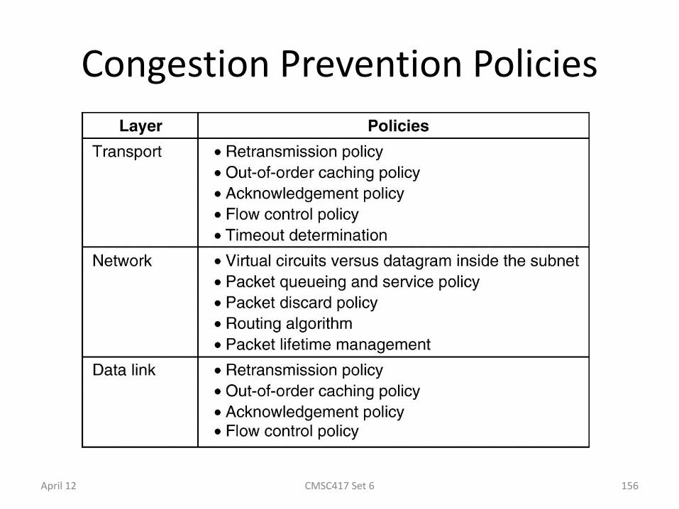
Congestion Prevention Policies
Policies that affect congestion.
5-26
April 12 CMSC417 Set 6 156
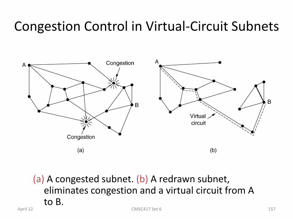
Congestion Control in Virtual-Circuit Subnets
(a) A congested subnet. (b) A redrawn subnet, eliminates congestion and a virtual circuit from A to B.
April 12 CMSC417 Set 6 157
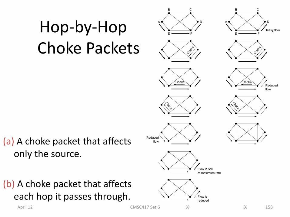
Hop-by-Hop Choke Packets
(a) A choke packet that affects only the source.
(b) A choke packet that affects each hop it passes through.
April 12 CMSC417 Set 6 158

Jitter Control
(a) High jitter. (b) Low jitter. April 12 CMSC417 Set 6 159

Quality of Service
• Application requirements
• Traffic shaping
• Packet scheduling
• Admission control
• Integrated services
• Differentiated services
April 12 CMSC417 Set 6 160
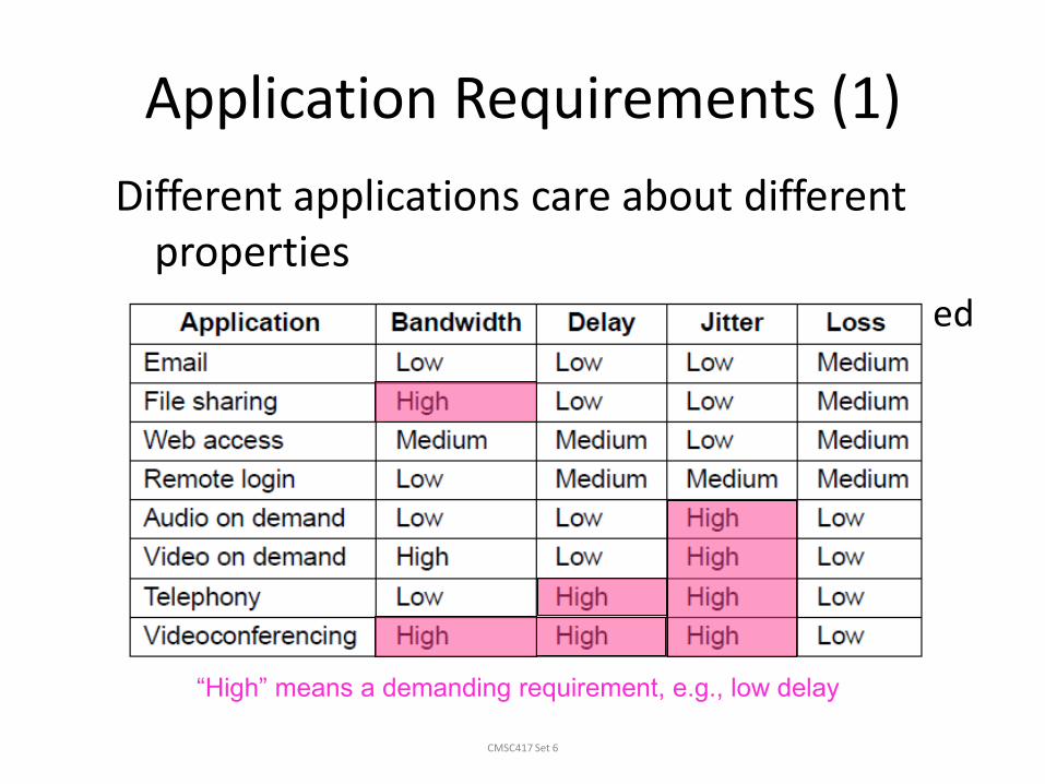
Application Requirements (1)
CMSC417 Set 6
Different applications care about different properties
– We want all applications to get what they need
.
“High” means a demanding requirement, e.g., low delay
Application Requirements (2)
CMSC417 Set 6
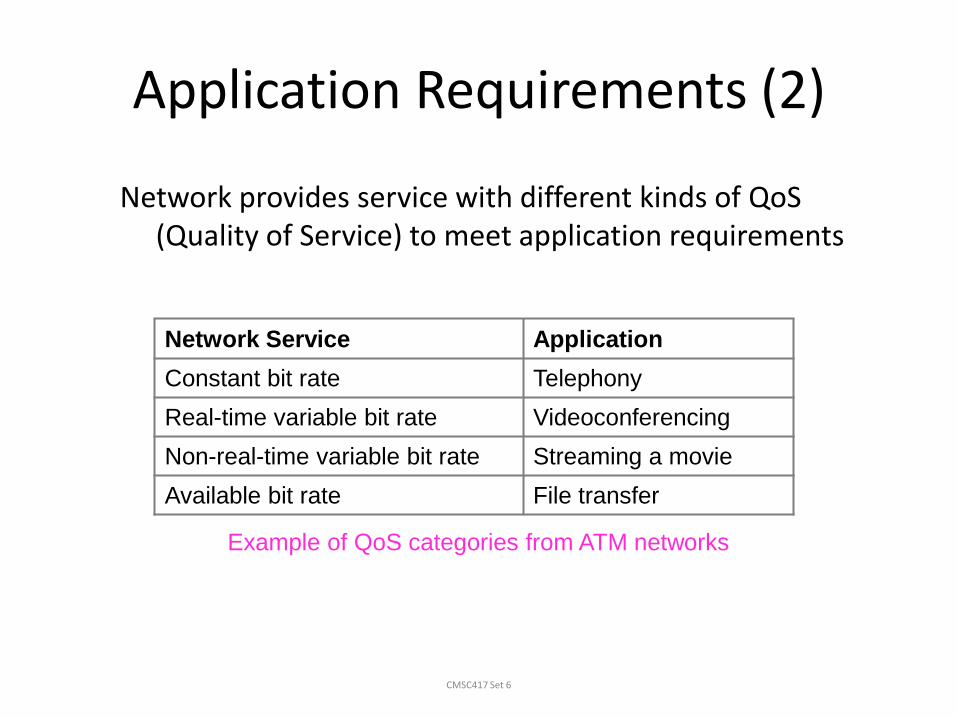
Network provides service with different kinds of QoS (Quality of Service) to meet application requirements
Network Service Application
Constant bit rate Telephony
Real-time variable bit rate Videoconferencing
Non-real-time variable bit rate Streaming a movie
Available bit rate File transfer
Example of QoS categories from ATM networks

Categories of QoS and Examples
1.Constant bit rate
• Telephony
2.Real-time variable bit rate
• Compressed videoconferencing
3.Non-real-time variable bit rate
• Watching a movie on demand
4.Available bit rate
• File transfer
April 12 CMSC417 Set 6 163
Buffering
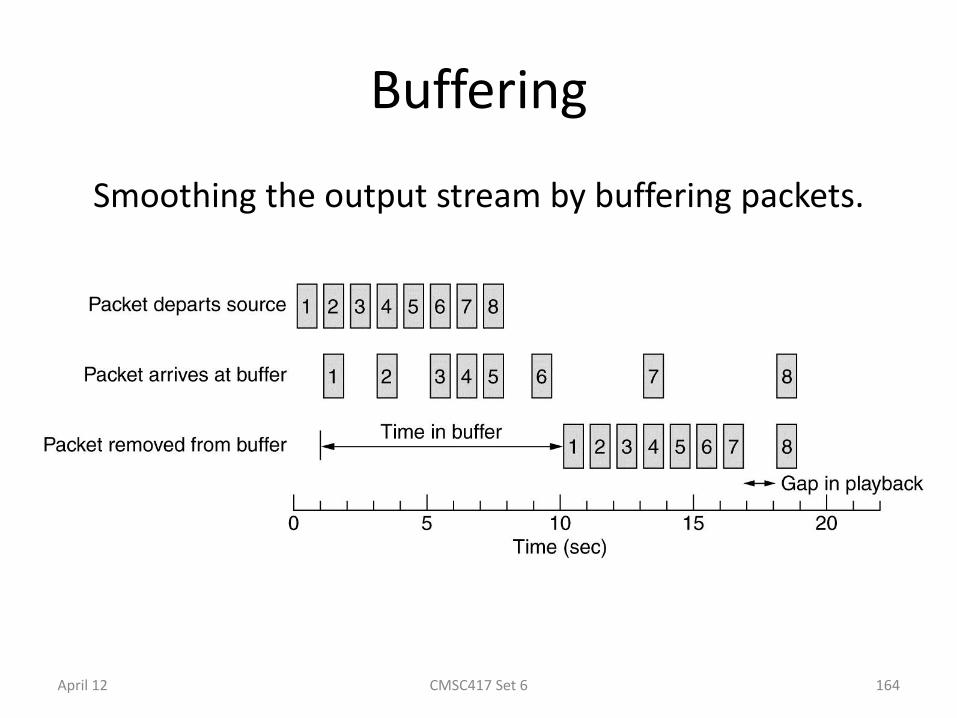
Smoothing the output stream by buffering packets.
April 12 CMSC417 Set 6 164
Traffic Shaping (1)
CMSC417 Set 6
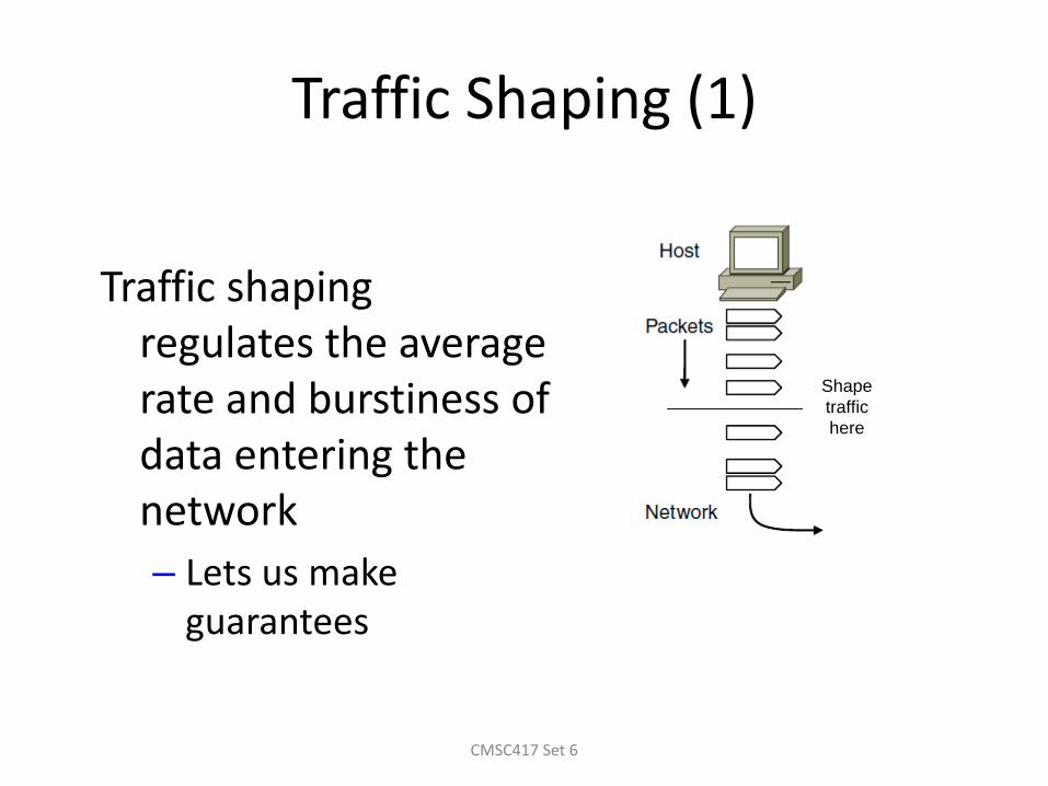
Traffic shaping regulates the average rate and burstiness of data entering the network
– Lets us make guarantees
Shape
traffic
here
Traffic Shaping (2)
CMSC417 Set 6
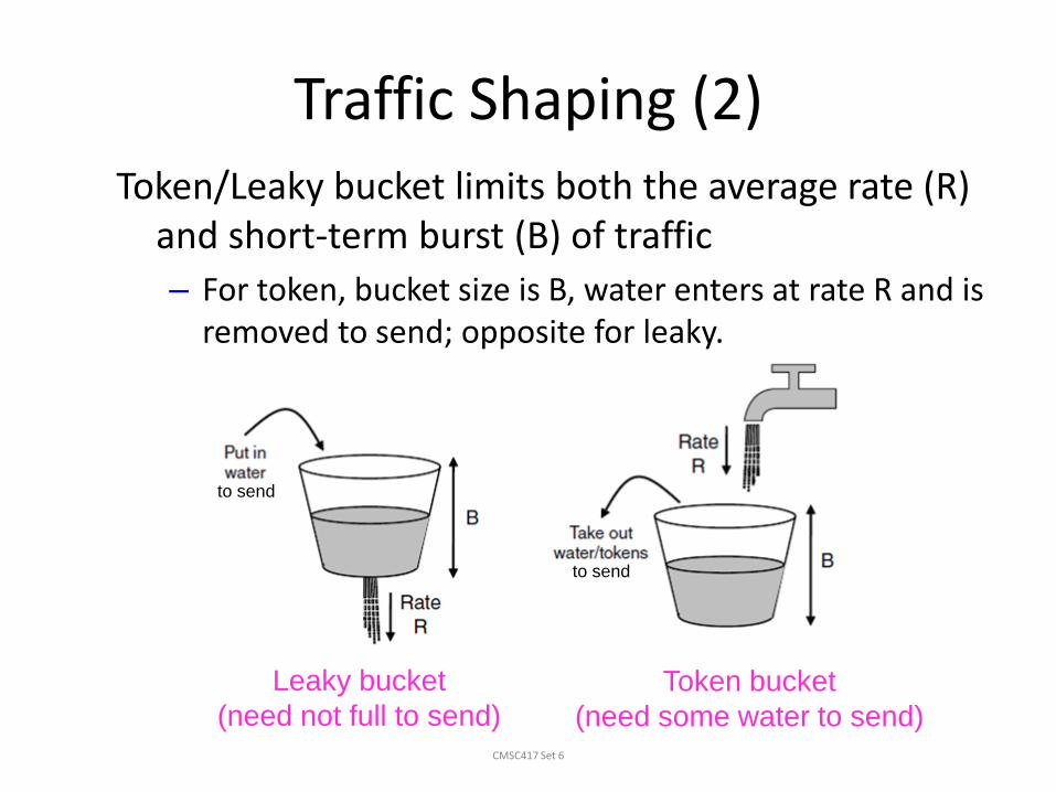
Token/Leaky bucket limits both the average rate (R) and short-term burst (B) of traffic
– For token, bucket size is B, water enters at rate R and is removed to send; opposite for leaky.
Leaky bucket
(need not full to send)
Token bucket
(need some water to send)
to send
to send

The Leaky Bucket Algorithm
(a) A leaky bucket with water. (b) a leaky bucket with packets. April 12 CMSC417 Set 6 167
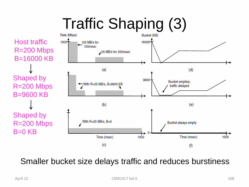
Traffic Shaping (3)
CMSC417 Set 6
Shaped by
R=200 Mbps
B=9600 KB
Shaped by
R=200 Mbps
B=0 KB
Host traffic
R=200 Mbps
B=16000 KB
Smaller bucket size delays traffic and reduces burstiness
April 12 168
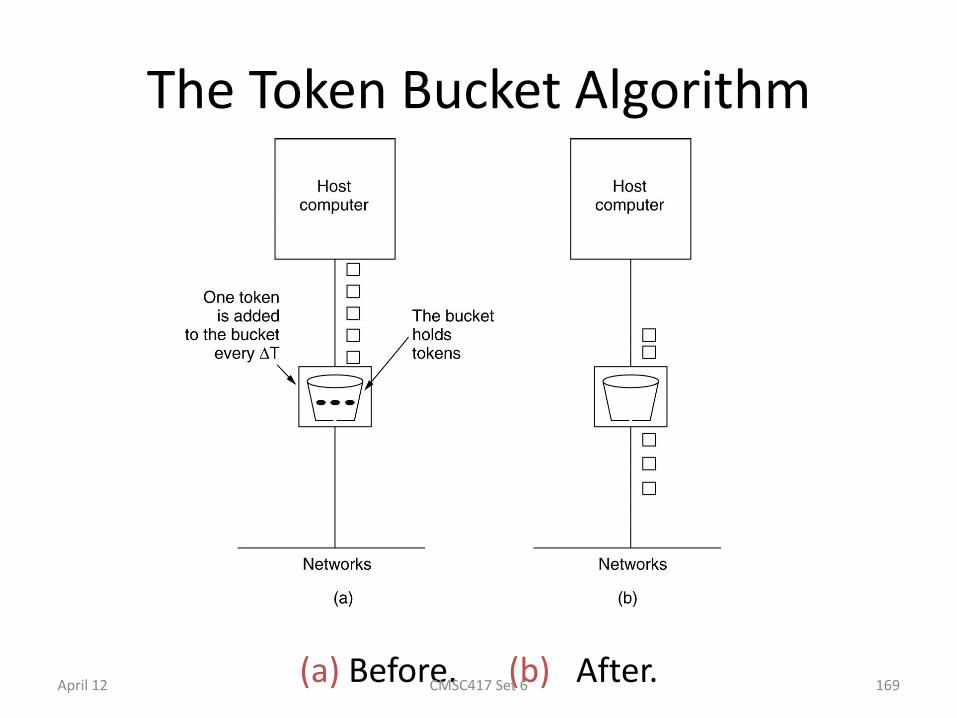
The Token Bucket Algorithm
(a) Before. (b) After.
5-34
April 12 CMSC417 Set 6 169
Packet Scheduling (1)
Kinds of resources can potentially be
reserved for different flows:
1. Bandwidth.
2. Buffer space.
3. CPU cycles.
April 12 CMSC417 Set 6 170

Packet Scheduling (1)
CMSC417 Set 6
Packet scheduling divides router/link resources among traffic flows with alternatives to FIFO (First In First Out)
Example of round-robin queuing
1 1 1
2 2
3 3 3

Packet Scheduling (2)
CMSC417 Set 6
Fair Queueing approximates bit-level fairness with different packet sizes; weights change target levels
– Result is WFQ (Weighted Fair Queueing)
Packets may be sent
out of arrival order
Finish virtual times determine
transmission order
Fi = max(Ai, Fi-1) + Li/W
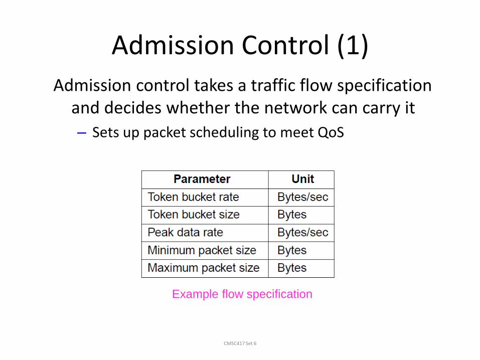
Admission Control (1)
CMSC417 Set 6
Admission control takes a traffic flow specification and decides whether the network can carry it
– Sets up packet scheduling to meet QoS
Example flow specification
Admission Control (2)
CMSC417 Set 6
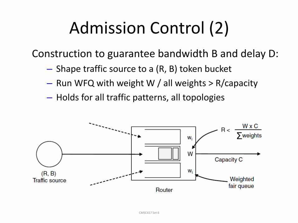
Construction to guarantee bandwidth B and delay D:
– Shape traffic source to a (R, B) token bucket
– Run WFQ with weight W / all weights > R/capacity
– Holds for all traffic patterns, all topologies
Integrated Services (1)
CMSC417 Set 6
Design with QoS for each flow; handles multicast traffic.
Admission with RSVP (Resource reSerVation Protocol):
– Receiver sends a request back to the sender
– Each router along the way reserves resources
– Routers merge multiple requests for same flow
– Entire path is set up, or reservation not made

RSVP-The ReSerVation Protocol
(a) A network, (b) The multicast spanning tree for host 1.
(c) The multicast spanning tree for host 2. April 12 CMSC417 Set 6 176

Integrated Services (2)
CMSC417 Set 6
R3 reserves flow
from S1 R3 reserves flow
from S2
R5 reserves flow from S1;
merged with R3 at H
Merge
April 12 177
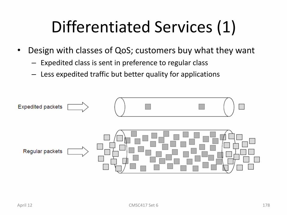
Differentiated Services (1) • Design with classes of QoS; customers buy what they want
– Expedited class is sent in preference to regular class
– Less expedited traffic but better quality for applications
CMSC417 Set 6 April 12 178
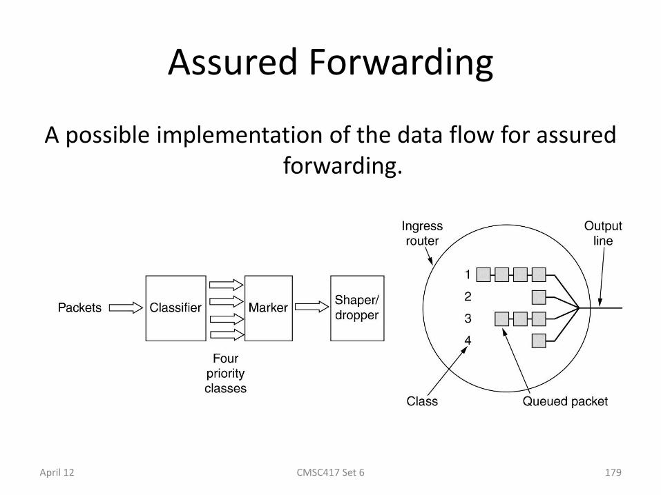
Assured Forwarding
A possible implementation of the data flow for assured forwarding.
April 12 CMSC417 Set 6 179
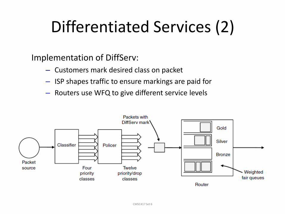
Differentiated Services (2)
CMSC417 Set 6
Implementation of DiffServ: – Customers mark desired class on packet
– ISP shapes traffic to ensure markings are paid for
– Routers use WFQ to give different service levels
The Network Layer in the Internet
• The IP Protocol
• IP Addresses
• Internet Control Protocols
• OSPF – The Interior Gateway Routing Protocol
• BGP – The Exterior Gateway Routing Protocol
• Internet Multicasting
• Mobile IP
• IPv6 April 12 CMSC417 Set 6 181
Internetworking
CMSC417 Set 6
Internetworking joins multiple, different networks into a single larger network
– How networks differ »
– How networks can be connected »
– Tunneling »
– Internetwork routing »
– Packet fragmentation »
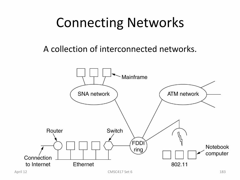
Connecting Networks
A collection of interconnected networks.
April 12 CMSC417 Set 6 183
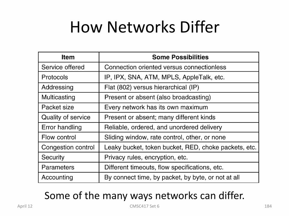
How Networks Differ
Some of the many ways networks can differ.
5-43
April 12 CMSC417 Set 6 184
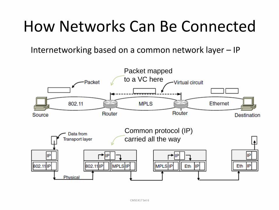
How Networks Can Be Connected
CMSC417 Set 6
Internetworking based on a common network layer – IP
Packet mapped
to a VC here
Common protocol (IP)
carried all the way

Concatenated Virtual Circuits
Internetworking using concatenated virtual circuits. April 12 CMSC417 Set 6 186

Connectionless Internetworking
A connectionless internet. April 12 CMSC417 Set 6 187

Tunneling
Tunneling a packet from Paris to London.
April 12 CMSC417 Set 6 188
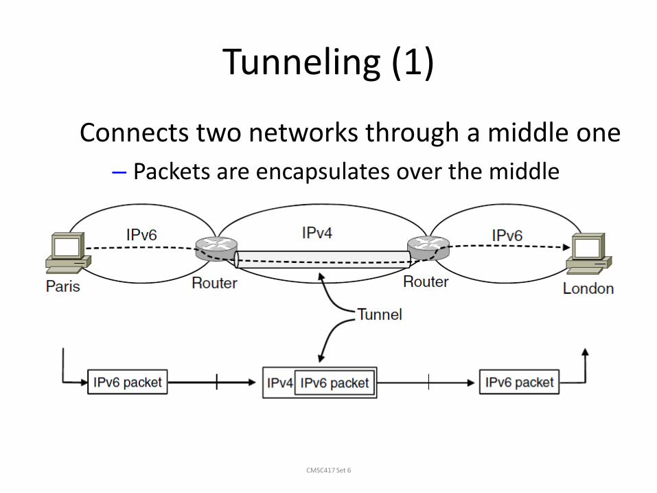
Tunneling (1)
CMSC417 Set 6
Connects two networks through a middle one
– Packets are encapsulates over the middle
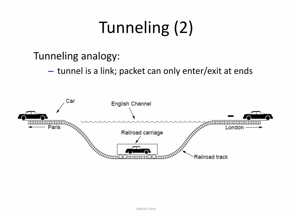
Tunneling (2)
CMSC417 Set 6
Tunneling analogy:
– tunnel is a link; packet can only enter/exit at ends
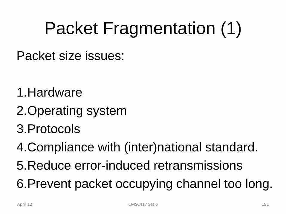
Packet Fragmentation (1)
Packet size issues:
1.Hardware
2.Operating system
3.Protocols
4.Compliance with (inter)national standard.
5.Reduce error-induced retransmissions
6.Prevent packet occupying channel too long.
April 12 CMSC417 Set 6 191
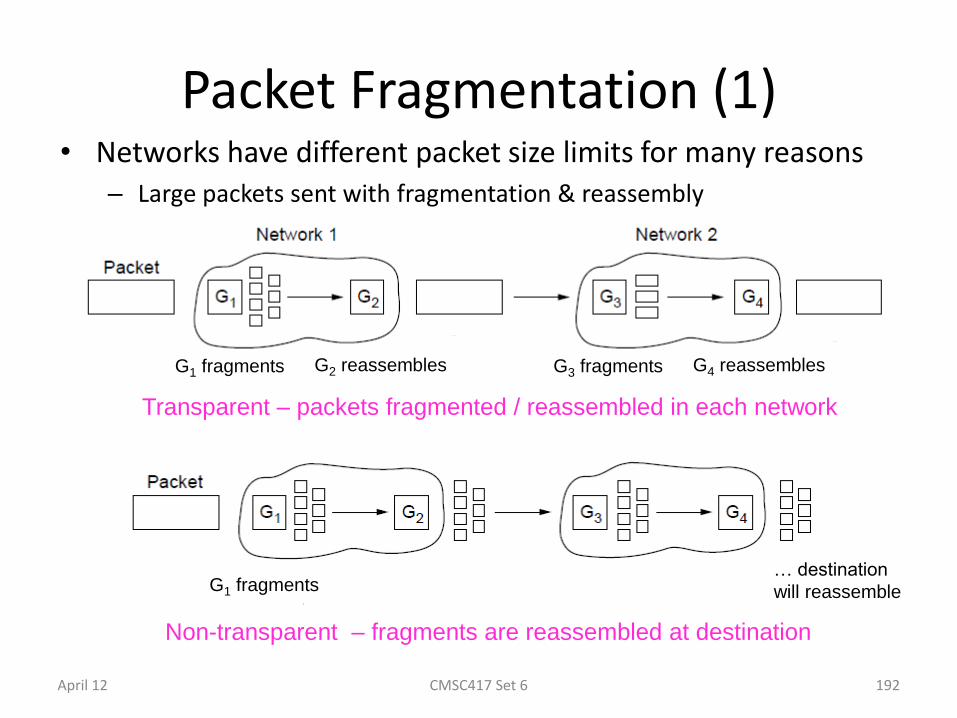
Packet Fragmentation (1) • Networks have different packet size limits for many reasons
– Large packets sent with fragmentation & reassembly
CMSC417 Set 6
G1 fragments G2 reassembles
Transparent – packets fragmented / reassembled in each network
Non-transparent – fragments are reassembled at destination
G3 fragments G4 reassembles
G1 fragments … destination
will reassemble
April 12 192
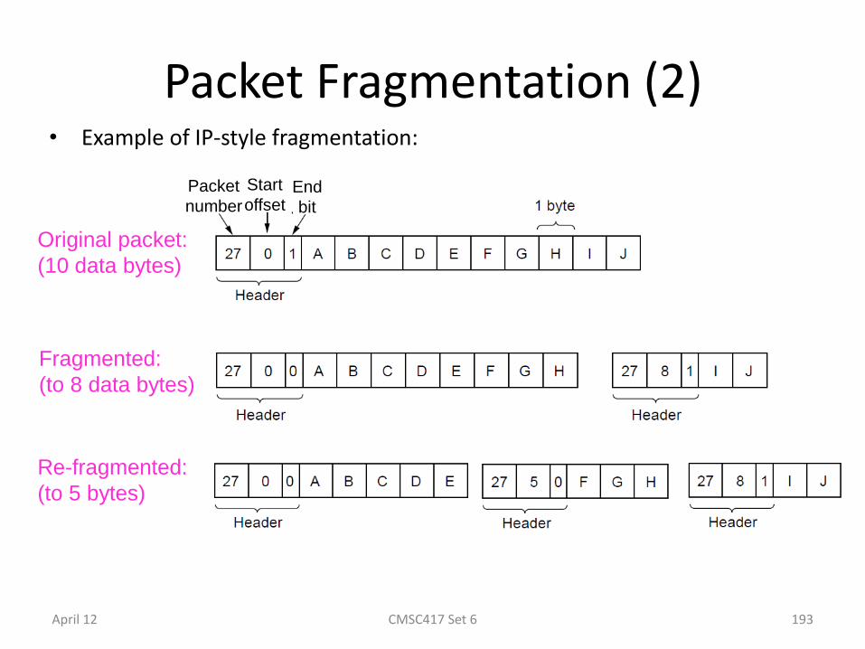
Packet Fragmentation (2) • Example of IP-style fragmentation:
CMSC417 Set 6
Packet
number
Start
offset End
bit
Original packet:
(10 data bytes)
Fragmented:
(to 8 data bytes)
Re-fragmented:
(to 5 bytes)
April 12 193
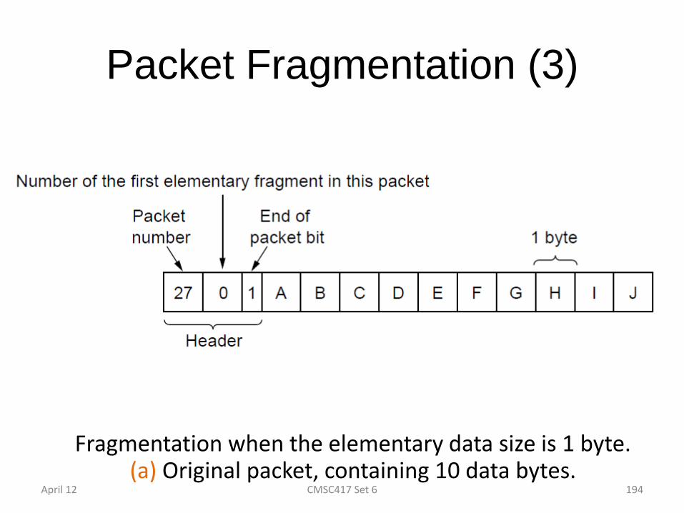
Packet Fragmentation (3)
Fragmentation when the elementary data size is 1 byte. (a) Original packet, containing 10 data bytes.
April 12 CMSC417 Set 6 194
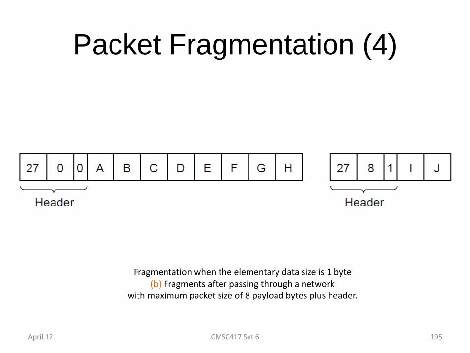
Packet Fragmentation (4)
Fragmentation when the elementary data size is 1 byte (b) Fragments after passing through a network
with maximum packet size of 8 payload bytes plus header.
April 12 CMSC417 Set 6 195
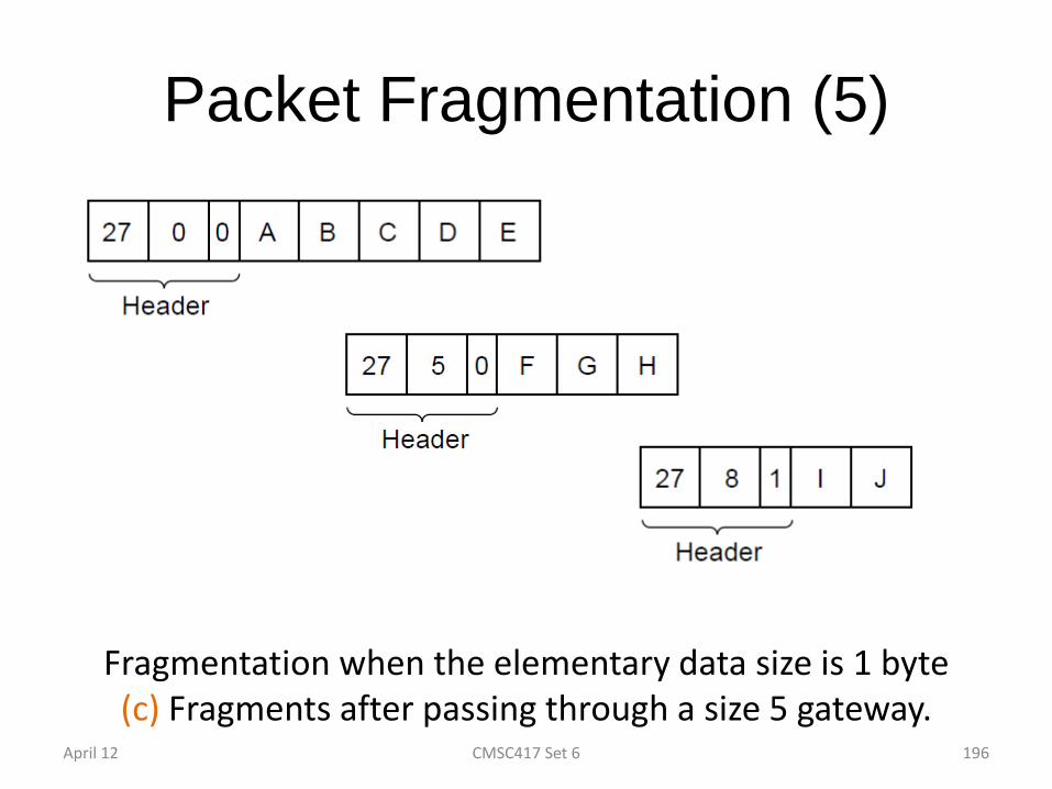
Packet Fragmentation (5)
Fragmentation when the elementary data size is 1 byte (c) Fragments after passing through a size 5 gateway.
April 12 CMSC417 Set 6 196
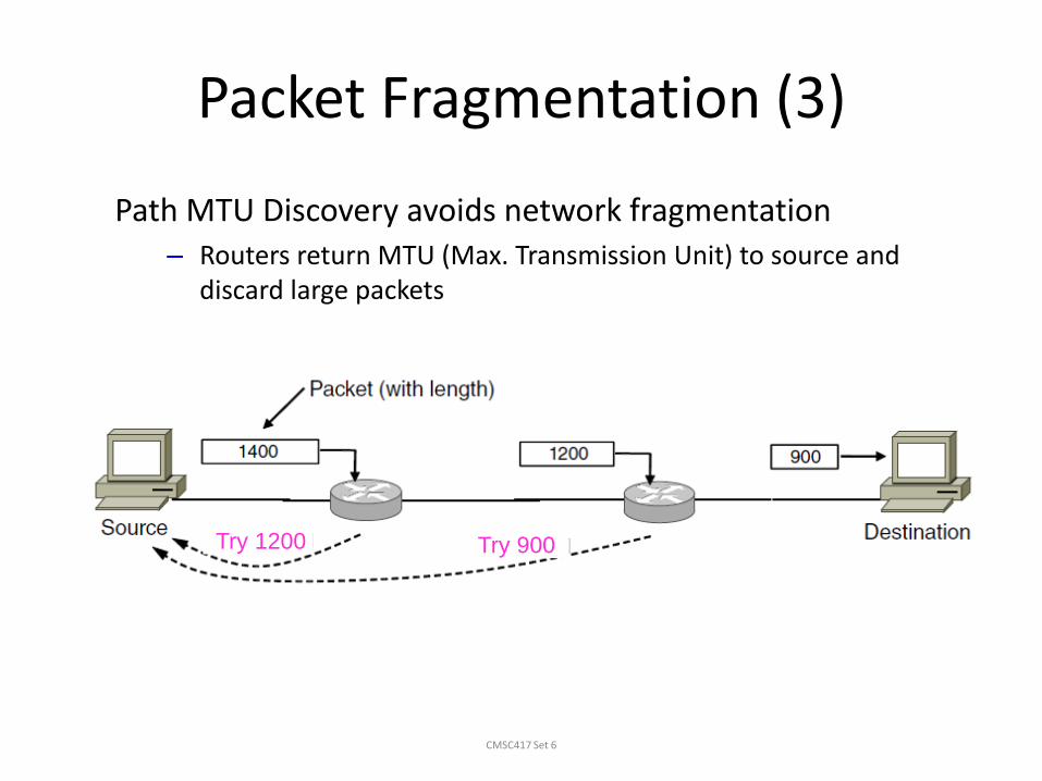
Packet Fragmentation (3)
CMSC417 Set 6
Path MTU Discovery avoids network fragmentation – Routers return MTU (Max. Transmission Unit) to source and
discard large packets
Try 1200 Try 900
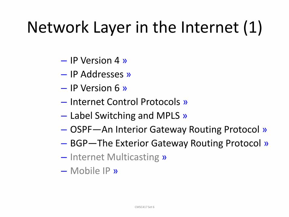
Network Layer in the Internet (1)
CMSC417 Set 6
– IP Version 4 »
– IP Addresses »
– IP Version 6 »
– Internet Control Protocols »
– Label Switching and MPLS »
– OSPF—An Interior Gateway Routing Protocol »
– BGP—The Exterior Gateway Routing Protocol »
– Internet Multicasting »
– Mobile IP »
Network Layer in the Internet (2)
CMSC417 Set 6
IP has been shaped by guiding principles: • Make sure it works
• Keep it simple
• Make clear choices
• Exploit modularity
• Expect heterogeneity
• Avoid static options and parameters
• Look for good design (not perfect)
• Strict sending, tolerant receiving
• Think about scalability
• Consider performance and cost
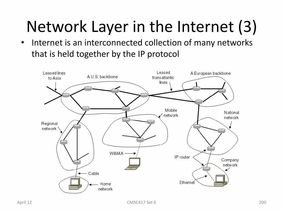
Network Layer in the Internet (3) • Internet is an interconnected collection of many networks
that is held together by the IP protocol
CMSC417 Set 6 April 12 200
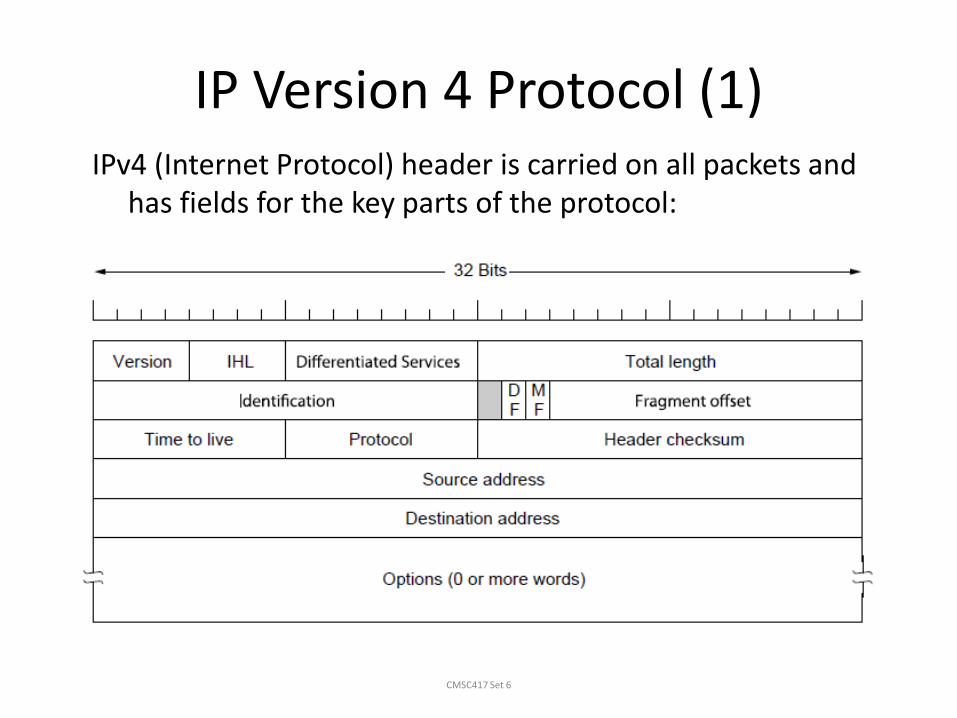
IP Version 4 Protocol (1)
CMSC417 Set 6
IPv4 (Internet Protocol) header is carried on all packets and has fields for the key parts of the protocol:
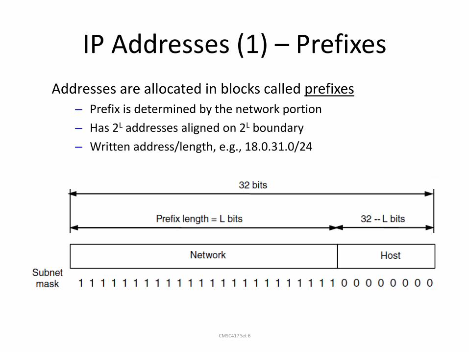
IP Addresses (1) – Prefixes
CMSC417 Set 6
Addresses are allocated in blocks called prefixes – Prefix is determined by the network portion
– Has 2L addresses aligned on 2L boundary
– Written address/length, e.g., 18.0.31.0/24
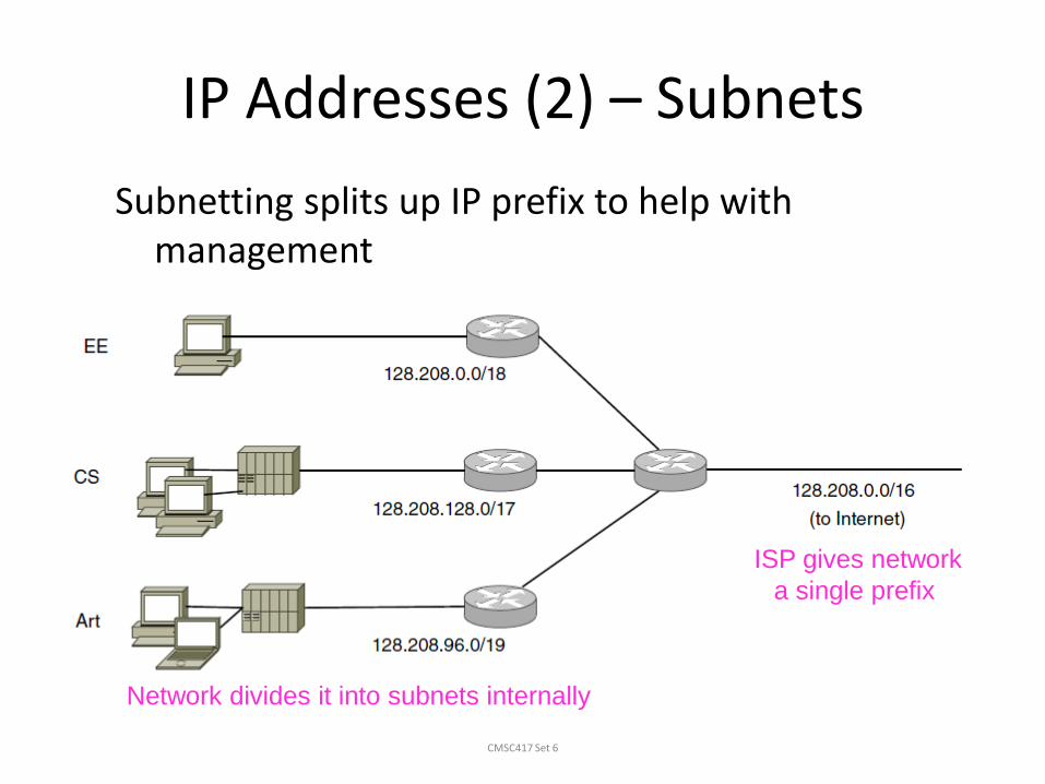
IP Addresses (2) – Subnets
CMSC417 Set 6
Subnetting splits up IP prefix to help with management
– Looks like a single prefix outside the network
Network divides it into subnets internally
ISP gives network
a single prefix
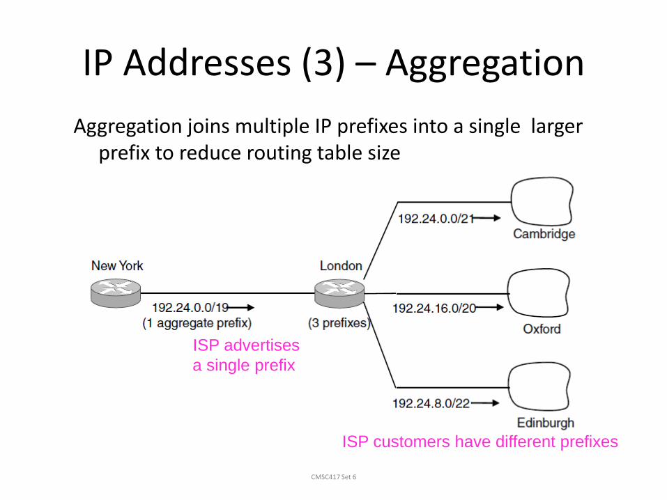
IP Addresses (3) – Aggregation
CMSC417 Set 6
Aggregation joins multiple IP prefixes into a single larger prefix to reduce routing table size
ISP customers have different prefixes
ISP advertises
a single prefix

IP Addresses (4) – Longest Matching Prefix
CMSC417 Set 6
Packets are forwarded to the entry with the longest matching prefix or smallest address block – Complicates forwarding but adds flexibility
Main prefix goes
this way
Except for
this part!
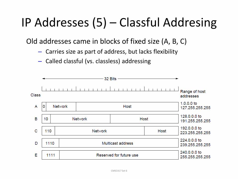
IP Addresses (5) – Classful Addresing
CMSC417 Set 6
Old addresses came in blocks of fixed size (A, B, C) – Carries size as part of address, but lacks flexibility
– Called classful (vs. classless) addressing
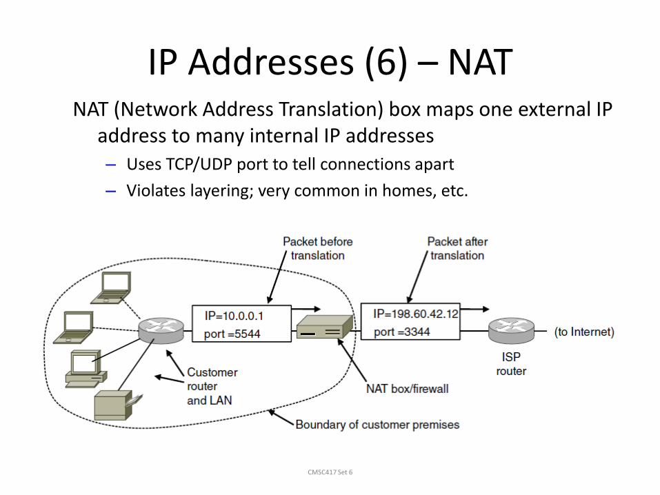
IP Addresses (6) – NAT
CMSC417 Set 6
NAT (Network Address Translation) box maps one external IP address to many internal IP addresses – Uses TCP/UDP port to tell connections apart
– Violates layering; very common in homes, etc.
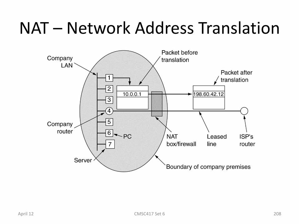
NAT – Network Address Translation
Placement and operation of a NAT box.
April 12 CMSC417 Set 6 208
IP Version 6 (1)
CMSC417 Set 6
Major upgrade in the 1990s due to impending address exhaustion, with various other goals:
• Support billions of hosts
• Reduce routing table size
• Simplify protocol
• Better security
• Attention to type of service
• Aid multicasting
• Roaming host without changing address
• Allow future protocol evolution
• Permit coexistence of old, new protocols, …
Deployment has been slow & painful, but may pick up pace now that addresses are all but exhausted

IP Version 6 (2 )
CMSC417 Set 6
IPv6 protocol header has much longer addresses (128 vs. 32 bits) and is simpler (by using extension headers)
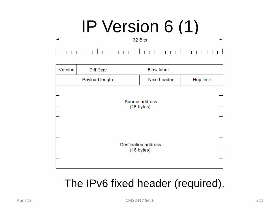
IP Version 6 (1)
The IPv6 fixed header (required).
April 12 CMSC417 Set 6 211

IP Version 6 (2)
IPv6 extension headers
April 12 CMSC417 Set 6 212

IP Version 6 (3)
The hop-by-hop extension header for large datagrams (jumbograms).
April 12 CMSC417 Set 6 213
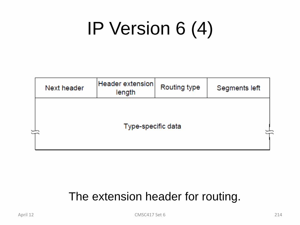
IP Version 6 (4)
The extension header for routing.
April 12 CMSC417 Set 6 214
Internet Control Protocols (1)
CMSC417 Set 6
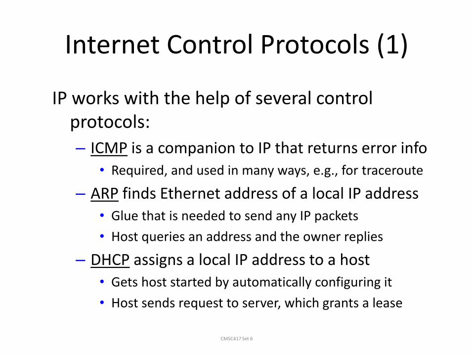
IP works with the help of several control protocols:
– ICMP is a companion to IP that returns error info
• Required, and used in many ways, e.g., for traceroute
– ARP finds Ethernet address of a local IP address
• Glue that is needed to send any IP packets
• Host queries an address and the owner replies
– DHCP assigns a local IP address to a host
• Gets host started by automatically configuring it
• Host sends request to server, which grants a lease
Internet Control Protocols (2)
CMSC417 Set 6
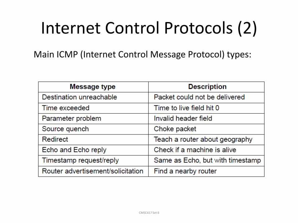
Main ICMP (Internet Control Message Protocol) types:
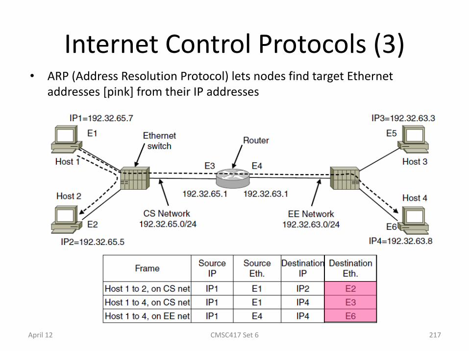
Internet Control Protocols (3) • ARP (Address Resolution Protocol) lets nodes find target Ethernet
addresses [pink] from their IP addresses
CMSC417 Set 6 April 12 217
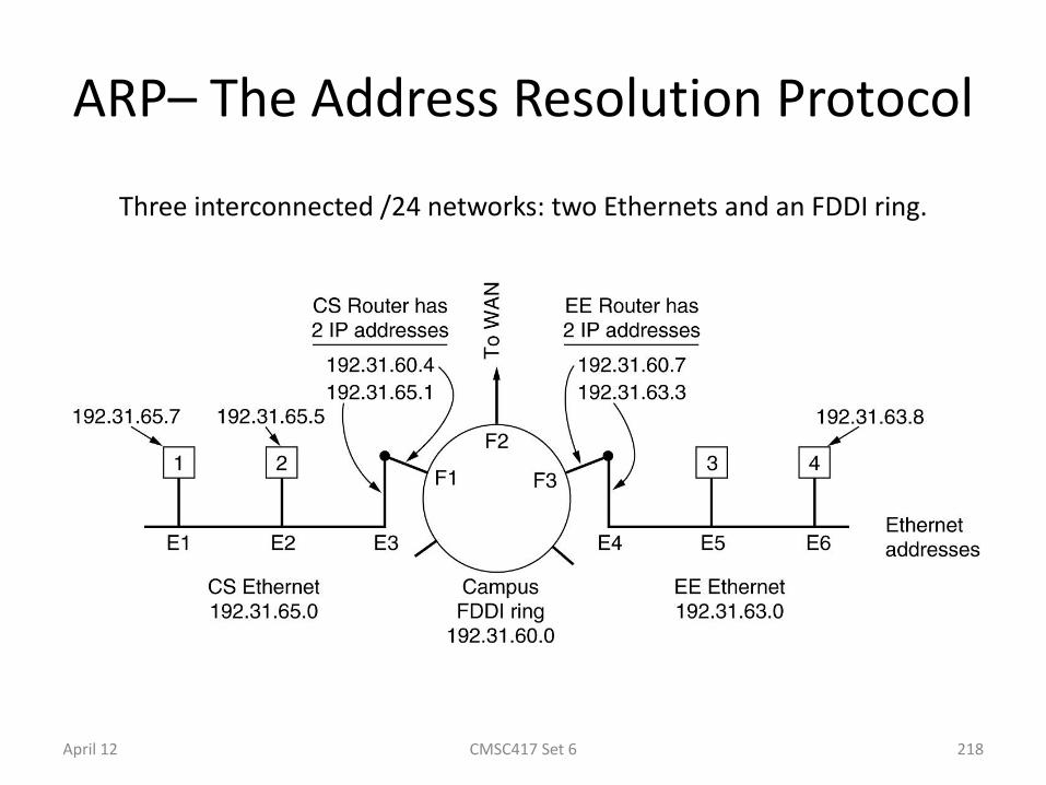
ARP– The Address Resolution Protocol
Three interconnected /24 networks: two Ethernets and an FDDI ring.
April 12 CMSC417 Set 6 218

Dynamic Host Configuration Protocol
Operation of DHCP.
April 12 CMSC417 Set 6 219
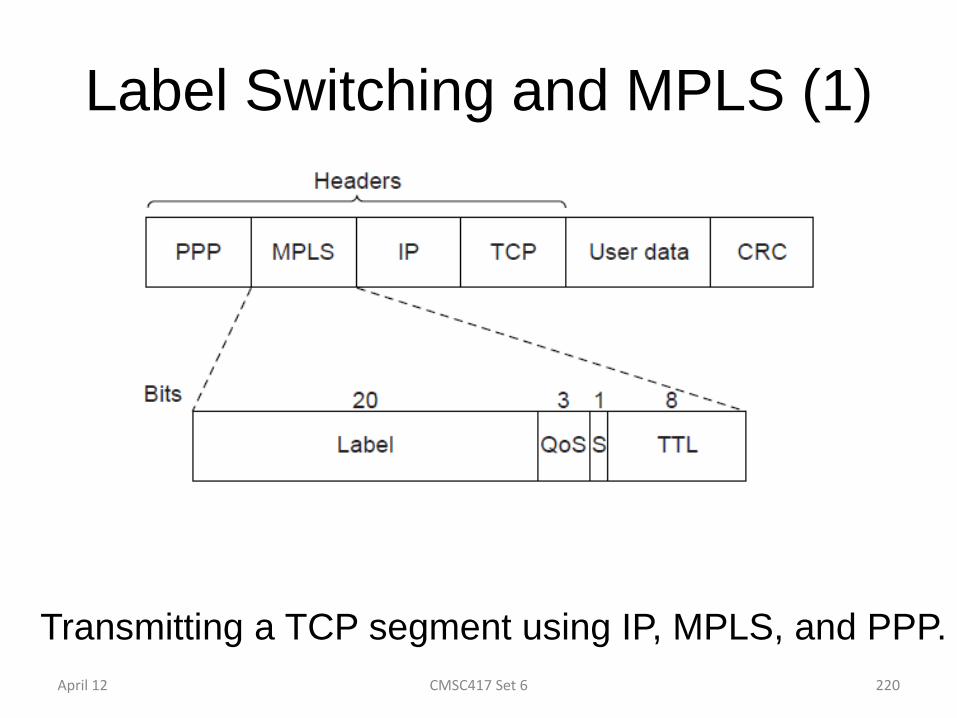
Label Switching and MPLS (1)
Transmitting a TCP segment using IP, MPLS, and PPP.
April 12 CMSC417 Set 6 220
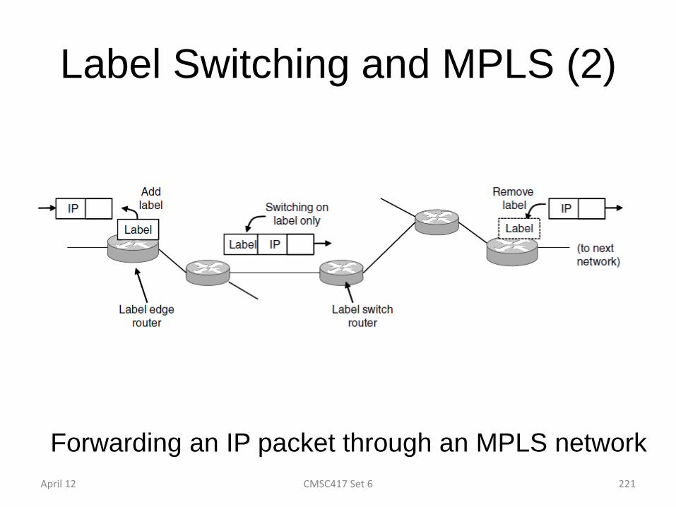
Label Switching and MPLS (2)
Forwarding an IP packet through an MPLS network
April 12 CMSC417 Set 6 221
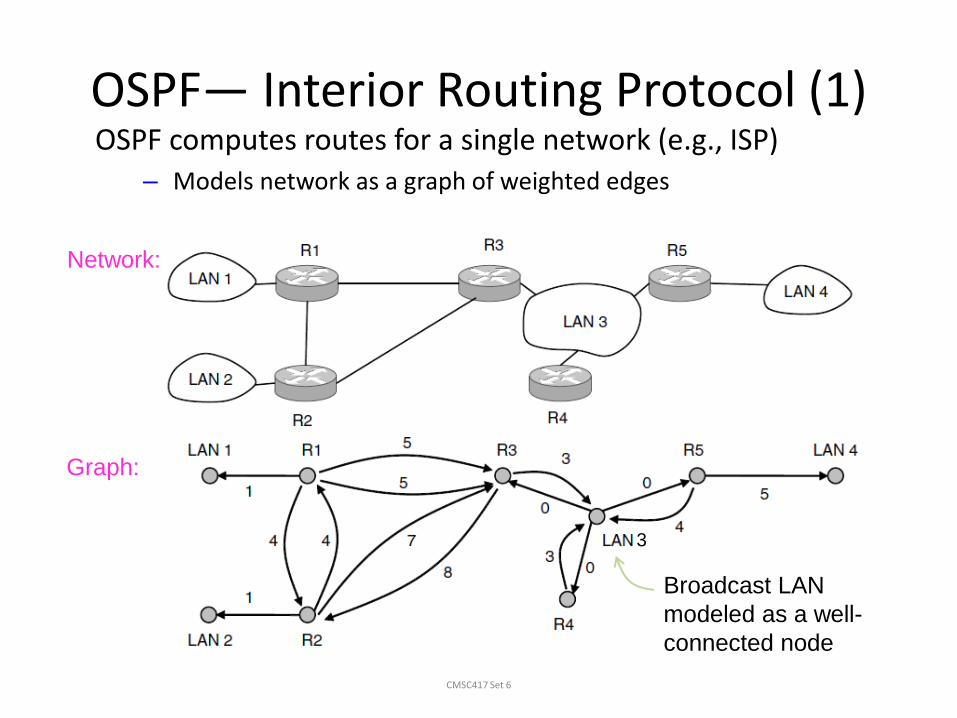
OSPF— Interior Routing Protocol (1)
CMSC417 Set 6
OSPF computes routes for a single network (e.g., ISP) – Models network as a graph of weighted edges
Network:
Graph:
Broadcast LAN
modeled as a well-
connected node
3

OSPF— Interior Routing Protocol (2)
CMSC417 Set 6
OSPF divides one large network (Autonomous System) into areas connected to a backbone area – Helps to scale; summaries go over area borders
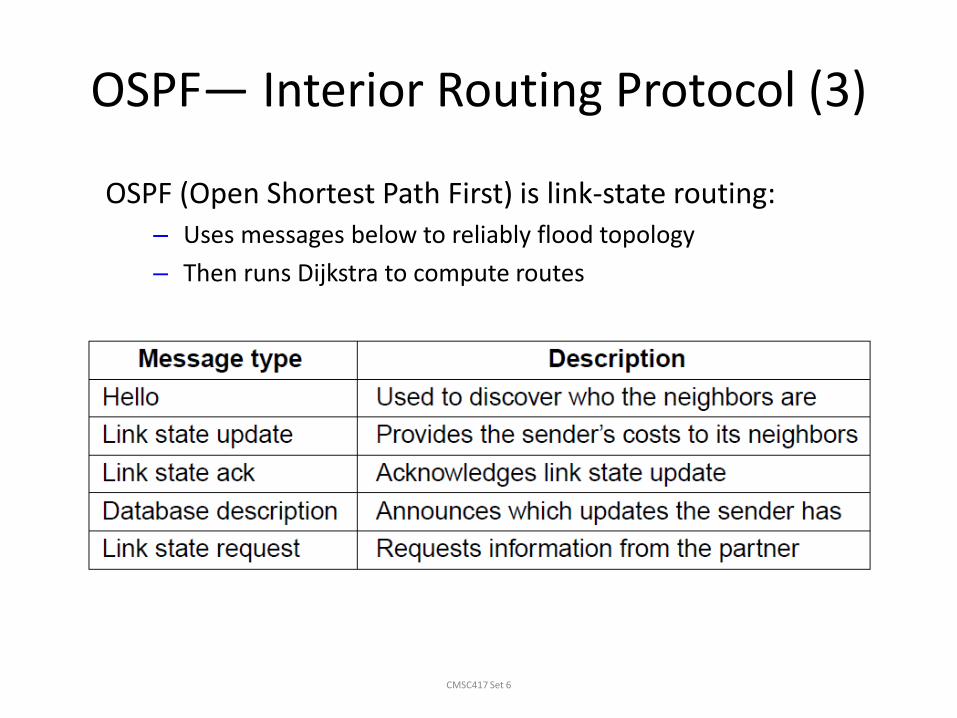
OSPF— Interior Routing Protocol (3)
CMSC417 Set 6
OSPF (Open Shortest Path First) is link-state routing: – Uses messages below to reliably flood topology
– Then runs Dijkstra to compute routes

BGP— Exterior Routing Protocol (1)
CMSC417 Set 6
BGP (Border Gateway Protocol) computes routes across interconnected, autonomous networks
– Key role is to respect networks’ policy constraints
Example policy constraints: • No commercial traffic for educational network
• Never put Iraq on route starting at Pentagon
• Choose cheaper network
• Choose better performing network
• Don’t go from Apple to Google to Apple

BGP— Exterior Routing Protocol (2)
CMSC417 Set 6
Common policy distinction is transit vs. peering: – Transit carries traffic for pay; peers for mutual benefit
– AS1 carries AS2↔AS4 (Transit) but not AS3 (Peer)
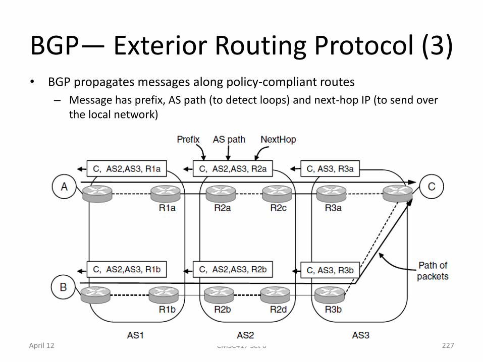
BGP— Exterior Routing Protocol (3) • BGP propagates messages along policy-compliant routes
– Message has prefix, AS path (to detect loops) and next-hop IP (to send over the local network)
CMSC417 Set 6 April 12 227