computer science & information technology 31aircconline.com/csit/csit431.pdf · hamdouche...
TRANSCRIPT

Computer Science & Information Technology 31


Natarajan Meghanathan
Jan Zizka (Eds)
Computer Science & Information Technology
The Sixth International Conference on Networks & Communications
(NeTCoM 2014)
Chennai, India, December 27 ~ 28 - 2014
AIRCC

Volume Editors
Natarajan Meghanathan,
Jackson State University, USA
E-mail: [email protected]
Jan Zizka,
Mendel University in Brno, Czech Republic
E-mail: [email protected]
ISSN: 2231 - 5403
ISBN: 978-1-921987-19-9
DOI : 10.5121/csit.2014.41301 - 10.5121/csit.2014.41316
This work is subject to copyright. All rights are reserved, whether whole or part of the material is
concerned, specifically the rights of translation, reprinting, re-use of illustrations, recitation,
broadcasting, reproduction on microfilms or in any other way, and storage in data banks.
Duplication of this publication or parts thereof is permitted only under the provisions of the
International Copyright Law and permission for use must always be obtained from Academy &
Industry Research Collaboration Center. Violations are liable to prosecution under the
International Copyright Law.
Typesetting: Camera-ready by author, data conversion by NnN Net Solutions Private Ltd.,
Chennai, India

Preface
The Sixth International Conference on Networks & Communications (NeTCoM 2014) was held in
Chennai, India, during December 27 ~ 28, 2014. International Conference on Computer Science and
Information Technology (CSIT-2014), Sixth International Conference on Applications of Graph
Theory in Wireless Ad hoc Networks & Sensor Networks (GRAPH-HOC 2014) and Second
International Conference of Security, Privacy and Trust Management (SPTM 2014). The conferences
attracted many local and international delegates, presenting a balanced mixture of intellect from the
East and from the West.
The goal of this conference series is to bring together researchers and practitioners from academia and
industry to focus on understanding computer science and information technology and to establish new
collaborations in these areas. Authors are invited to contribute to the conference by submitting articles
that illustrate research results, projects, survey work and industrial experiences describing significant
advances in all areas of computer science and information technology.
The NeTCoM-2014, CSIT-2014, GRAPH-HOC-2014, SPTM-2014 Committees rigorously invited
submissions for many months from researchers, scientists, engineers, students and practitioners related
to the relevant themes and tracks of the workshop. This effort guaranteed submissions from an
unparalleled number of internationally recognized top-level researchers. All the submissions
underwent a strenuous peer review process which comprised expert reviewers. These reviewers were
selected from a talented pool of Technical Committee members and external reviewers on the basis of
their expertise. The papers were then reviewed based on their contributions, technical content,
originality and clarity. The entire process, which includes the submission, review and acceptance
processes, was done electronically. All these efforts undertaken by the Organizing and Technical
Committees led to an exciting, rich and a high quality technical conference program, which featured
high-impact presentations for all attendees to enjoy, appreciate and expand their expertise in the latest
developments in computer network and communications research.
In closing, NeTCoM-2014, CSIT-2014, GRAPH-HOC-2014, SPTM-2014 brought together
researchers, scientists, engineers, students and practitioners to exchange and share their experiences,
new ideas and research results in all aspects of the main workshop themes and tracks, and to discuss
the practical challenges encountered and the solutions adopted. The book is organized as a collection
of papers from the NeTCoM-2014, CSIT-2014, GRAPH-HOC-2014, SPTM-2014.
We would like to thank the General and Program Chairs, organization staff, the members of the
Technical Program Committees and external reviewers for their excellent and tireless work. We
sincerely wish that all attendees benefited scientifically from the conference and wish them every
success in their research. It is the humble wish of the conference organizers that the professional
dialogue among the researchers, scientists, engineers, students and educators continues beyond the
event and that the friendships and collaborations forged will linger and prosper for many years to
come.
Natarajan Meghanathan
Jan Zizka

Organization
General Chair
Jagannathan Sarangapani Missouri University of Science and
Technology, USA
Natarajan Meghanathan Jackson State University, USA
Program Committee Members
Abdel Salhi University of Essex, United Kingdom
Abdulrahman Yarali Murray state university, USA
Ahlem Drif Computer science Department, Algeria
Ahmed Ezz Eldin Khaled Cairo University, Egypt
Alexander Ferworn Ryerson University, Canada
Ali Alawneh Philadelphia University, Jordan
Alireza mahini Islamic Azad University-Gorgan, Iran
Almir Pereira Guimaraes Federal University of Alagoas, Brazil
Alvin Lim Auburn University, USA
Antonio Ruiz-Martinez University of Murcia, Spain
Asmaa Shaker Ashoor Babylon University, Iraq
Bob Natale MITRE, USA
Cathryn Peoples University of Ulster, United Kingdom
Chih-Lin Hu National Central University, Taiwan
Chin-Chih Chang Chung Hua University,Taiwan
Christos Politis Kingston University, UK
Cristina Ribeiro University of Waterloo, Canada
Dac-Nhuong Le Haiphong University, Vietnam
Daqiang Zhang Nanjing Normal University, China
David C. Wyld Southeastern Louisiana University, USA
Dhinaharan Nagamalai Wireilla net solutions PTY ltd, Australia
Doina Bein The Pennsylvania State University,USA
Ehsan Heidari Islamic Azad University Doroud Branch, Iran
Emmanuel Jammeh University of Plymouth, United Kingdom
Farshchi S.M.R Seyyed Mohammd Reza Farshchi, Iran
Firdous Imam Imam unversity Riyadh, Saudi Arabia
Gary Campbell University College of the Caribbean, Jamaica
Ghaida Al-Suhail Basrah Univirsity, Iraq
Hamadouche M USDB, Algeria
Hamdouche Maamar Université Saad Dahlab de Blida, Algeria
Hamza Aldabbas De Montfort University, UK
Han Cong Vinh Nguyen Tat Thanh University, Vietnam
Hangwei Western Reserve University, USA
Hao-En Chueh Yuanpei University, Taiwan, R.O.C.
Hazem Al-Najjar Misurata university, Libya

Hazem M. AL-Najjar Taibah University, Kingdom of Saudi Arabia
Hossein Jadidoleslamy University of Zabol, Zabol, Iran
Houcine Hassan Univeridad Politecnica de Valencia, Spain
Ibrahim EL BITAR Cole Mohammadia d,Ingenieurs, Morocco
Ioannis Karamitsos University of Aegean,Greece
Isa Maleki Islamic Azad University, Iran
Islam Atef Alexandria University, Egypt
Iwan Adhicandra University of Pisa, Italy
J. K. Mandal University of Kalyani, India
Jacques DEMERJIAN Communications & Systems, France.
Jadidoleslamy University of Zabol, Iran
Jaime Lloret Polytechnic University of Valencia, Spain
John Woods University of Essex, United Kingdom
Jose Neuman de Souza Federal University of Ceara, Brazil
Josip Lorincz University of Split, Croatia
Juan Jose Martinez Castillo Ayacucho University, Venezuela
Kayhan Erciyes Izmir University,Turkey
Keivan Borna Kharazmi University, Iran
Ken Guild University of Essex, United Kingdom
Korchiyne redouan Ibn Tofail University, Morocco
Laiali Almazaydeh University of Bridgeport, USA
M. NADEEM BAIG Riyadh, K.S.A
M.Mohamed Ashik Salalah College of Technology,Oman
Mahdi Aiash Middlesex University, UK
Mahi Lohi University of Westminster, UK
Malamati Louta University of Western Macedonia, GREECE
Malka N. Halgamuge The University of Melbourne, Australia
Martin Fleury University of Essex, United Kingdom
Mohamed Fahad AlAjmi King Saud University, Saudi Arabia
Mohamed Hassan American University of Sharjah, UAE
Mohammed Ghanbari University of Essex, United Kingdom
Moses Ekpenyong University of Edinburgh, Nigeria
Mounir gouiouez Laboratory Modeling and Simulation, Morocco
Muhammad Naufal Bin Mansor University Malaysia Perlis, Malaysia
Nadia Qadri University of Essex, United Kingdom
Natarajan Meghanathan Jackson State University, USA
Nazmus Saquib University of Manitoba, Canada
Omar Almomani Jadara University, Jordan
Parminder S Reel The Open University, United Kingdom
Paulo Martins Maciel Federal University of Pernambuco, Brazil
Paulo R.L. Gondim University of Brasilia,Brazil
Phan Cong Vinh NTT University, Vietnam
Quan (Alex) Yuan University of Wisconsin-Stevens Point, USA
Rabie Ramadan Cairo University, Egypt
Rachida Dssouli Concordia University, Canada
Raed alsaqour Universiti Kebangsaan Malaysia, Malaysia
Ramayah Universiti Sains Malaysia,Malaysia
Roy Eagleson Western University, Canada
Rushed Kanawati LIPN - university Paris 13, France

Sajid Hussain Fisk University, USA
Sattar B. Sadkhan University of Babylon,Iraq
Selma Boumerdassi Cnam/cedric, France
Selwyn Piramuthu University of Florida
Serguei A. Mokhov Concordia University, Canada
Seyyed Reza Khaze Islamic Azad University, Iran
Sherif S. Rashad Morehead State University, USA
Sherimon P.C., Arab Open University,Sultanate of Oman
Suleyman Kondakci Izmir University of Economics, Turkey
Tinatin Mshvidobadze Gori University, Georgia
Vuda Sreenivasa Rao Bahir Dar University, Ethiopia
Wichian Sittiprapaporn Mahasarakham University, Thailand
XU Mengxi Nanjing Institute of Technology, China
Yannick Le Moullec Aalborg University,Denmark
Yasir Qadri University of Essex, United Kingdom
Yasser Hashemi Islamic Azad University, Iran
Yingchi Mao Hohai University, China
Zuqing Zhu Cisco Systems, USA
Technically Sponsored by
Networks & Communications Community (NCC)
Computer Science & Information Technology Community (CSITC)
Digital Signal & Image Processing Community (DSIPC)
Organized By
Academy & Industry Research Collaboration Center (AIRCC)

TABLE OF CONTENTS
Sixth International Conference on Networks & Communications
(NeTCoM 2014)
Deployment Driven Security Configuration for Virtual Networks…..........….. 01 - 13
Ramaswamy Chandramouli
Performance Analysis of Resource Scheduling in LTE Femtocells
Networks………………………………………………………………...………… 15 - 25
Samia Dardouri and Ridha Bouallegue
MC CDMA Performance on Single Relay Cooperative System by Diversity
Technique in Rayleigh Fading Channel………..............................................….. 27 - 39
Gelar Budiman, Ali Muayyadi and Rina Pudji Astuti
Highly Accurate Log Skew Normal Approximation to the Sum of Correlated
Lognormals………............................................................................................….. 41 - 52
Marwane Ben Hcine and Ridha Bouallegue
Fitting the Log Skew Normal to the Sum of Independent Lognormals
Distribution………............................................................................................….. 53 - 67
Marwane Ben Hcine and Ridha Bouallegue
Selective Image Encryption Using DCT with AES Cipher……....................….. 69 - 77
Belazi Akram, Benrhouma Oussama, Hermassi Houcemeddine and Belghith Safya
Dynamic Optimization of Overlap and Add Length Over MBOFDM System
Based on SNR and CIR Estimate……….........................................................….. 79 - 96
Nouri Naziha and Bouallegue Ridha
EDD Clustering Algorithm for Wireless Sensor Networks……....................... 97 - 104
Awatef Ben Fradj Guiloufi, Salim El Khediri, Nejah Nasri and
Abdennaceur Kachouri
VideoConferencing Web Application for Cardiology Domain Using
FLEX/J2EE Technologies………....................................................................... 105 - 117
Imen Debbabi and Ridha Bouallegue
Alamouti OFDM/OQAM Systems with Time Reversal Technique…......….. 119 - 130
Ilhem Blel and Ridha Bouallegue

International Conference on Computer Science and Information
Technology (CSIT-2014)
Issues, Challenges and Solutions : Big Data Mining…...............................….. 131 - 140
Jaseena K.U and Julie M. David
DT-BAR : A Dynamic ANT Recommender to Balance the Overall
Prediction Accuracy for all Users…………………………….…………....….. 141 - 151
Abdelghani Bellaachia and Deema Alathel
Medical Diagnosis Classification Using Migration Based Differential
Evolution Algorithm…..................................................................................….. 153 - 163
Htet Thazin Tike Thein and Khin Mo Mo Tun
A New Survey on Biclustering of Microarray Data…………………........….. 165 - 183
Haifa Ben Saber and Mourad Elloumi
Sixth International Conference on Applications of Graph Theory in
Wireless Ad hoc Networks & Sensor Networks
(GRAPH-HOC 2014)
TTACCA : Two-Hop Based Traffic Aware Congestion Control Algorithm
for Wireless Sensor Networks…...................................................................….. 185 - 194
Prabha R, Prashanth Kumar Gouda, Manjula S H, K R Venugopal and L M Patnaik
Second International Conference of Security, Privacy and Trust
Management (SPTM 2014)
Predictive Cyber Security Analytics Framework : A Nonhomogenous
MARKOV Model for Security Quantification…........................................….. 195 - 209
Subil Abraham and Suku Nair

Natarajan Meghanathan et al. (Eds) : NeTCoM, CSIT, GRAPH-HOC, SPTM - 2014
pp. 01–13, 2014. © CS & IT-CSCP 2014 DOI : 10.5121/csit.2014.41301
DEPLOYMENT-DRIVEN SECURITY
CONFIGURATION FOR VIRTUAL
NETWORKS
Ramaswamy Chandramouli
Computer Security Division, Information Technology Laboratory
National Institute of Standards & Technology
Gaithersburg, MD, USA [email protected]
ABSTRACT
Virtualized Infrastructures are increasingly deployed in many data centers. One of the key
components of this virtualized infrastructure is the virtual network – a software-defined
communication fabric that links together the various Virtual Machines (VMs) to each other and
to the physical host on which the VMs reside. Because of its key role in providing connectivity
among VMs and the applications hosted on them, Virtual Networks have to be securely
configured to provide the foundation for the overall security of the virtualized infrastructure in
any deployment scenario. The objective of this paper is to illustrate a deployment-driven
methodology for deriving a security configuration for Virtual Networks. The methodology
outlines two typical deployment scenarios, identifies use cases and their associated security
requirements, the security solutions to meet those requirements, the virtual network security
configuration to implement each security solution and then analyzes the pros and cons of each
security solution.
KEYWORDS
Virtualized Infrastructure, Virtual Machine, Virtual Network, Security Configuration, Software
Defined Network
1. INTRODUCTION
Virtualized infrastructures are increasingly deployed in many data centers, driven by cost,
efficiency, scalability and in some cases security considerations. The term virtualized
infrastructure, in the context of this paper, includes the following: the physical host or server that
is virtualized (called Virtualized Host), the Hypervisor software, the Virtual Machines (VMs)
residing on a virtualized host, the software-defined virtual network that is configured inside a
virtualized host, middleware and management tools specific to the virtualized environment, the
hardware/software components relating to storage, the common networking components of the
data center such as physical Network Interface Cards (physical NIC), switches (physical and
virtual), routers, firewalls, load balancers, application delivery controllers etc.
One of the key components of this virtualized infrastructure is the virtual network [1] – a
software-defined communication fabric that links together the various Virtual Machines (VMs) to
each other and to the physical host on which the VMs reside. The VMs are instantiated and
managed by a piece of software called “Hypervisor” which in turn is installed in many instances

2 Computer Science & Information Technology (CS & IT)
directly on a physical computing hardware. We will refer to the physical computing hardware on
which the hypervisor is installed as Virtualized Host.
It is in fact the hypervisor that provides the API and the functional code necessary to define and
configure a virtual network linking the various VMs with each other and to the virtualized host
where they (Hypervisor and the VMs) all reside. Since the term “Virtual Network” in the context
of networking as a whole is an overloaded term, it is good to clarify its semantics in the context
of the virtualized infrastructure discussed in this paper. In our context, the term virtual network
encompasses the two aspects: (a) Software-enabled NIC Virtualization and (b) Data path
Virtualization. A brief explanation of these two aspects follows:
Software-enabled NIC Virtualization [2]: Here a physical Network Interface Card (pNIC) in a
virtualized host is shared among many Virtual Operating Systems (OSs) (called Guest OS,
Virtual Machines or Domains depending upon the product offering). This sharing is possible
through a software-defined artifact called Virtual NIC (or vNIC), which is a software emulation
of a physical NIC. Each vNIC is defined within a Virtual OS and the latter is therefore called the
client of vNIC. Each vNIC may be assigned its own dedicated IP and MAC addresses. If the
Virtual OSs (clients of vNIC) run a server software (e.g., Web Server, DNS Server or Firewall),
they are also referred to as “Virtual Servers”. The bridging of these vNICs or multiplexing of the
traffic from different vNICs (and hence different VMs or Virtual Servers) for achieving the goal
of sharing physical NICs is achieved using a software-defined switch called virtual switch
(vSwitch in some product offerings) [3]. Links between vNICs and virtual switches are software-
emulated links and so are the links between virtual switches and physical NICs (the later are also
called uplinks).
Data path Virtualization [2]: The software-emulated links created by NIC virtualization above
can be virtualized using a capability in the virtual switches. This type of link virtualization is
different from virtualization of links found in physical channels (using multiplexing or creation of
virtual circuit) where virtualization happens at the channel. In data path virtualization,
virtualization of links happens at the network node level (i.e., virtual switch). These virtual
switches (vSwitches) have the capability to define dynamic multiple port groups within it (just
like ports in a physical switch). These port groups are tagged with what are known as Virtual
LAN (VLAN) IDs [4]. These tags or labels are used by virtual switches to create multiple virtual
links (data paths). Thus VLAN tags achieve two different objectives – to share the same
infrastructure (e.g., the LAN infrastructure or communication channel) as well as creating data
paths in the broadcast domain.
In Summary, the virtual network in the context of this paper is a “software-emulated network
which generates traffic that is injected into the real world through a non-virtual/non-emulated
physical NIC” [2] and has the following building blocks:
• Virtual Servers (Clients of vNICs)
• Virtual NICs (vNICs)
• Virtual Switches (vSwitch)
• Virtual Links and
• Physical NICs (pNICs).
In addition to the above components, we also include external physical switches/routers attached
to virtualized hosts (more specifically to the physical NICs of the hosts) also under the umbrella
of the “virtual network” since they play a role in configuration of the virtual network (e.g., inter-
VLAN routing). Other components such as VLAN ID/Port Group (in the Virtual Switch),
Software-defined firewalls & IDS/IPS installed as Virtual Security Appliance (VSA), Load
Balancers etc (sometimes packaged as Virtual Appliances) are also included since they are
artifacts used in a virtual network configuration as well.

Computer Science & Information Technology (CS & IT) 3
Having settled on the semantics for the virtual network, let us turn our attention to the role of
virtual networks in a virtualized infrastructure. While the hypervisor kernel provides the process-
level isolation for the VMs, it is the virtual network that provides the connectivity between the
VMs and the applications hosted on them. Hence, secure configuration of the virtual network
forms the foundation for the security of the entire virtualized infrastructure. Two significant
deployment scenarios for a large virtualized infrastructure are:
• Hosting Multi-tier applications (with extensive connectivity between components
containing various application tiers) with a large user base, large volume of data or high
volume of transactions or combination of all three
• Offering an Infrastructure as a Service (IaaS) public cloud service.
In this scenario, VMs belonging to different cloud service clients could be potentially co-
residents in a single virtualized host of the infrastructure.
It must be emphasized that the two deployment scenarios stated above are not mutually exclusive.
For example, a 3-tier application (consists of Web Server, Application Server & Database Server
tiers) may be hosted on three different groups of VMs either by the enterprise itself (as part of its
internal IT resources) or by a cloud service client (if the virtualized infrastructure is used for
offering a public cloud service). In the former case, the virtualized infrastructure and all the VMs
are owned by the enterprise while in the latter case, the ownership of the VMs is with the cloud
service client while the virtualized infrastructure is owned by the cloud service provider.
The objective of this paper is to illustrate a methodology for obtaining a secure virtual network
configuration based on deployment scenarios cited above. The methodology is based on
identifying the typical set of use cases in the deployment scenarios. Section 2 lists the steps of the
methodology and identifies the various use cases. Section 3 is the core material for this paper as it
describes the steps of the methodology used to derive security configuration for a virtual network
and also analyzes the pros and cons of the underlying security solution. Section 4 outlines the
benefits of the methodology.
2. METHODOLOGY FOR DERIVING VIRTUAL NETWORK SECURITY
CONFIGURATION
The methodology for deriving a virtual network security configuration has the following key
steps:
• STEP 1: Identify the key use cases that result from the deployment scenarios stated in the
previous section. We consider only use cases that have an impact on virtual network
configuration parameters and identify those that are not within the scope of the
methodology.
• STEP 2: For each chosen use case, identify the associated security requirements and a
security solution that will meet the requirements.
• STEP 3: Identify and describe the virtual network security configuration operations that
will implement the security solutions and also analyze the pros and cons of those security
solutions.

4 Computer Science & Information Technology (CS & IT)
2.1 Choice of Use Cases in Virtualized Infrastructure Deployments
As already mentioned, we consider here only those use cases that are relevant from the virtual
network standpoint. Before identifying those use cases, we first provide here certain use cases
that get a lot of attention in deployments involving virtualized infrastructures [5], but do not
impact the virtual network configuration parameters. These use cases therefore are not considered
within the scope of our methodology.
• Building a VM image, versioning of VM images, maintaining the integrity of the VM
images both during storage and while using them for instantiating VM instances.
• Configuring the VM OS (or Guest OS)
• Configuring Endpoint (Virus & Malware) protection for VMs
• Providing Access Protection for accessing VMs from an external network
• Comprehensive Data Protection (Data in VM definition files and Application Data)
We now identify the typical set of use cases that may require virtual network configuration for
their secure implementation. All these use cases by and large pertain to one or both of the two
key components of the virtualized infrastructure: the Hypervisor and the VMs. They are:
• Managing the Hypervisor and the virtual network it spawns (e.g., VMs, Virtual
Switches/Port Groups/VLANs etc) (MH)
• Providing Selective Isolation/Connectivity between various applications/VMs (VM-CO)
3. IMPACT OF USE CASE OPERATIONS ON VIRTUAL NETWORK
SECURITY CONFIGURATION
In this section, we describe for each use case, the associated security requirements, the security
solutions that will meet the security requirements and the virtual network security configuration
operations that will implement each security solution and also analyze the pros and cons of each
of the security solutions.
3.1 Management of the Hypervisor (MH)
The set of management commands sent to the hypervisor includes those that are needed for
running a hypervisor as well those that are needed to create an application hosting environment
(Provisioning VM instances & Creating a Virtual Network configuration to support them).
Specifically these are the broad categories of commands sent to the hypervisor.
• Commands needed to set the hypervisor’s functional parameters (e.g., the CPU
scheduling algorithm it uses)
• The commands needed to define the topology of the virtual network (creation of virtual
switches, ports within each virtual switch and connections between vNICs provided
through virtual switches as well as connections from ports/virtual switches to physical
NICs of the virtualized host)
• Commands relating to operations on VMs (e.g,, Start, Stop & Pause VMs, Migrate a VM
from one Virtualized Host to another etc – these are sometimes called VM lifecycle
operations)
In some hypervisor architectures, the functions relating to VM Management (VM Lifecycle
operations) are offloaded to a dedicated, security hardened VM (sometimes called Management
VM). Regardless of this architectural variation, all hypervisors have an interface (called

Computer Science & Information Technology (CS & IT) 5
management interface) for sending these management commands. The obvious security
requirements (SR) considering the sensitive nature of the operations performed by the invocation
of these commands are:
• MH-SR-1: The sources from which these commands originate must be restricted to some
trusted sources
• MH-SR-2: The management commands must be sent securely - protecting their integrity
and sometimes confidentiality.
• MH-SR-3: The communication channels (data paths) carrying these management
commands must be logically isolated from channels carrying other types of traffic such
as the data/application related traffic.
Out of the three security requirements stated above, MH-SR-1 is met by restricting the set of
users who are authorized to invoke the hypervisor management commands to some trusted
administrators and by restricting the origin of the command packets to designated administrative
LANs within the enterprise [6]. For accomplishing this latter objective, a dedicated software-
defined firewall may have to be installed exclusively for protecting the management interface.
MH-SR-2 is met by establishing a secure communication protocol such as SSH with the
management interface and sending the management commands digitally signed and/or encrypted
[6]. Hence the only security requirement here that has to be met through a virtual network-based
security solution is MH-SR-3. The security solution (SS) for obtaining an isolated
communication channel exclusively dedicated to management commands (requirement MH-SR-
3) is:
• SS-1: Use a dedicated virtual network segment for sending all management commands to
the Hypervisor.
The virtual network security configuration operations to implement the above security solution
are:
• VN-SC-OP-1: Dedicate a VLAN for carrying just the hypervisor management traffic.
This is accomplished by creating a port of connection type console or kernel (depending
upon the hypervisor) on a virtual switch of the hypervisor and assigning a VLAN ID to
that port and associating the management interface (along with its IP address) with it. A
dedicated VLAN on a kernel-type port is also the preferred configuration option for
supporting VM Migration commands.
• VN-SC-OP-2: An added security assurance, in the pursuit of isolating management
traffic from all other traffic into the hypervisor, can be obtained by having a virtual
switch (vSwitch) just dedicated for defining the management VLAN with no other
connections.
Analysis of the security solution: A dedicated virtual network segment is just one of the three
security solutions for managing the hypervisor. It has to be augmented with administrator access
control, interface-protecting firewall and a secure communication protocol.
3.2 Providing Selective Isolation/Connectivity between various applications/VMs
(VM-CO)
In the previous section, the need for isolating the management traffic from the application traffic
was addressed. There is also a need to provide selective isolation among traffic pertaining to

6 Computer Science & Information Technology (CS & IT)
different applications running in VMs. This need is closely aligned with the two deployment
scenarios outlined in Section 1 as follows:
• Multi-tier Applications: The enterprise may run multiple multi-tier applications of
different sensitivity levels in VMs based on the type of data processed or the
functions/operations performed. In some instances, VMs need to be isolated based on the
Line of Business (LOB) and/or functional departments.
• Multiple Tenants on a Host: VMs belonging to different cloud service clients must be
logically isolated from one another to protect the integrity of data and applications hosted
on them. In many instances, there may be the need to provide logical isolation among
VMs belonging to the same cloud service client.
After isolating the VMs by the nature of the application (or LOB or Functional Department) or
cloud service client, it may be found that some business processes require that applications in the
VMs of one department/LOB may need to communicate or interact with applications in VMs of
other departments/LOBs. These twin security requirements (Selective Isolation and Connectivity)
are stated as follows:
• VM-SR-1: Traffic going into/emanating from VMs running sensitive applications must
be isolated from traffic pertaining to non-sensitive applications. Traffic among VMs
belonging to a Line of Business (LOB) or a functional department (e.g., Accounting,
Engineering etc) or a cloud service client must be isolated from corresponding traffic
from other LOBs, functional departments or cloud service clients respectively.
• VM-SR-2: Communication between VMs belonging to different logical groups
(Application Profile, LOB or Functional Department) must be enabled in some instances
but should be governed by a security policy.
The various security solutions that can meet the above requirements are:
• SS-2: Virtual Network Segmentation using VLAN IDs
• SS-3: Virtual Network Segmentation using VLAN IDs with Software Defined Network
(SDN) support
• SS-4: Control of Network traffic using Firewalls installed as Virtual Security Appliances
(VSA)
• SS-5: Control of Network traffic using Virtual Switches with SDN Support
A description of the above security solutions, the virtual network security configuration
operations needed to implement each of the solutions and performance characteristics of each of
these solutions are given below:
3.2.1 Virtual Network Segmentation using VLAN IDs
Isolation of traffic among VMs residing in a virtualized host (or in different hosts) is achieved by
segmentation of the virtual network and connecting the VMs (or Virtual Network Interface Cards
(vNICs)) to the corresponding port in the virtual switch tagged with the ID of that virtual network
segment. A common technology used for this purpose is the Virtual Local Area Network or
VLAN. Since the VMs in a virtualized host are connected to virtual switches, the ports in the
virtual switches are tagged with VLAN IDs and the VMs designated for a particular VLAN

Computer Science & Information Technology (CS & IT) 7
segment are assigned (connected) to the corresponding virtual switch port. The necessary
operations for achieving the requisite virtual network security configuration are:
• VN-SC-OP-3: Identify the set of VMs that belongs to a specific cloud service client
(tenant) or Line of Business (LOB) or functional department and assign them to a new
VLAN (VLAN ID). Also identify the set of virtualized hosts that are targets for hosting
them.
• VN-SC-OP-4: Define a new VLAN using the interface that your LAN management
software provides.
• VN-SC-OP-5: Define/Identity virtual switches on the target hosts (for identified VMs),
define/identify ports on those virtual switches and associate the new VLAN ID with
those switch ports. This type of ports is simply called VM portgroup in some
hypervisors. Connect the identified VMs (or the vNIC) to those portgroups.
• VN-SC-OP-6: The previous operation has configured the virtual switches inside the
virtualized hosts with the new VLAN. The same VLAN has to be configured on the
external physical switches connected to those virtualized hosts. This requires four
operations: (1) The new VLAN ID has to be added to the external switch’s VLAN
database; (2) At least one of the ports on that external switch must be enabled to support
traffic carrying that VLAN ID; (3) The port enabled for that VLAN ID must be
connected to the physical NIC of the virtualized host, and finally (4) that particular
physical NIC should be connected as the uplink port for the virtual switch on which the
new VLAN ID is defined.
This establishes a communication path from the vNIC of the VM to the virtual switch’s port (to
which the former is connected) and through its (the virtual switch) uplink port to the virtualized
host’s physical NIC and on to the external physical switch. One requirement needed for this
configuration is that the port on the external switch on which VLAN is enabled should be
configured as a trunk port (capable of receiving/forwarding traffic belonging to multiple
VLANs). Firewall rules can then defined on this external switch to provide selective connectivity
between different VLANs.
Analyzing the above security solution, we find the following limitations. They are [7]:
• There is a limit to the number of VLAN IDs that can be used (the figure is 4096)
• Configuring the virtual switches inside the virtualized hosts (where identified VMs are
hosted) as well as physical switches connected to the virtualized hosts for one or more
VLANs is a manual, time-consuming and error-prone process, part of which may have to
be repeated if application profile of VMs change.
• To enforce restrictions on inter-VLAN communication, the enforcement point is a
physical firewall or the physical switch. This requires routing all traffic originating from
or coming into a VM to the physical NIC of the virtualized host and on to the trunk port
of a external physical switch, thus increasing the latency of communication packets with
consequent increase in application response times.
3.2.2 Virtual Network Segmentation using VLAN IDs with SDN support
Before looking at this security solution, it would be good to review the architectural concepts
underlying SDN. SDN is an architectural concept that enables direct programmability of

8 Computer Science & Information Technology (CS & IT)
networks through open-source Standards-based APIs [8]. This capability is enabled by dividing
the functionality of a network device such as a switch or router into two distinct layers – the data
plane and control plane. The control plane is implemented by a software called SDN controller
and defines how data flows (i.e., how network messages/packets are forwarded and routed) while
the data plane performs the basic task of storing/forwarding packets based on entries in the
forwarding table. The SDN controller is often centralized (so that it controls data forwarding
functions of multiple data planes each associated with a network device) and communicates with
data planes through a standardized API (e.g., OpenFlow [9]). The interface to the data plane
(which in the SDN architecture is essentially is a network device with SDN support (such as a
SDN switch) is also called “Southbound Interface”. Similarly the SDN controller also can be
implemented to have an open interface, called the “Northbound Interface”. An architectural
diagram of a SDN is given in Figure 1 below:
Figure 1. SDN High Level Architecture
The SDN architecture can be leveraged to automate the creation of VLANs for isolating traffic
among VMs in the following way. First, the virtual switches that can be defined using the
hypervisor APIs should be capable of supporting SDN capabilities. An example is the open
vSwitch [10]. Secondly, there should be a SDN controller that can communicate with and control
all SDN supported virtual switches. With this set up, the Northbound interface exposed by SDN
controller can be used to send in commands to create the necessary VLANs (operation VN-SC-
OP-4) as well as send in information regarding VMs and their locations (virtualized hosts and
SDN virtual switches) pertaining to each VLAN. This information is used in the SDN controller
to generate commands, that is sent through the Southbound Interface for: (a) creating the
necessary port groups/VLAN tags on SDN supported switches and (b) connect the VMs to those
switch ports (operation VN-SC-OP-5). Similarly the tasks involved in VN-SC-OP-6 can also be
automated if the external physical switch is also a SDN switch.
This security solution presents the following advantages:
• Due to standardized interfaces and pre-programmed scripts, the creation of VLAN and
enabling the connectivity of VMs to the designated VLAN are automated thereby
reducing/eliminating the errors that could creep in manual configuration. The relevant

Computer Science & Information Technology (CS & IT) 9
interfaces are: (a) SDN controller interface (Northbound Interface) and (b) SDN
supported virtual switch interface (Southbound Interface).
• Similarly, the VLAN reconfiguration necessitated by VM migrations or change in
application profiles of VMs can also be automated using SDN interfaces.
• The VLAN ID limit of 4096 imposed by IEEE 802.1Q standard can be overcome by
creating packet forwarding rules in SDN controller based on MAC addresses to be placed
on virtual switches
3.2.3. Control of Network traffic using Firewalls installed as Virtual Security Appliances
In the virtualized infrastructure, network security using firewalls can be implemented in two
ways: (a) installing a firewall in each of the VMs to be protected or (b) installing a firewall at the
hypervisor-level to enforce traffic control rules for all VMs in that virtualized host. The latter
solution uses the hypervisor’s Virtual Machine Introspection (VMI) API. The configuration
operations for this solution are:
VN-SC-OP-7: Install a firewall as a Virtual Security Appliance (VSA) inside a hardened VM.
This appliance has the ability to enforce traffic restrictions on traffic going into any VM by virtue
of its access to the hypervisor’s VMI API. The packets for enforcement are fed into it by a
hypervisor kernel module that forwards all or selected (based on a set of rules) packets coming
into the vNIC of every VM in the virtualized host [11].
The performance characteristics of this security solution are:
• It does not consume the valuable CPU cycles in individual VMs which could otherwise
be used for running the business applications.
• All policies needed for the firewall can be defined centrally in the Virtual Infrastructure
Management server and then pushed in to the firewall VSA running in several virtualized
hosts.
• Firewall VSAs are capable of supporting sophisticated logic for traffic control rules such
as the ability to define security groups based on customized criteria.
3.2.4. Control of Network traffic using Virtual Switches with SDN Support
To implement this solution, the virtualized infrastructure should have a network with SDN
capabilities as described in 3.2.2. In this solution, traffic control using firewall like rules which
only allow packets based on the following values – A specific protocol (TCP or UDP), from port,
to port, A single IP address or range of IP addresses can be implemented directly on virtual
switches in a hypervisor instead of in a virtual security appliance (VSA) [12]. A set of VMs is
associated with a Security Group. A traffic control rule can be associated with one or more
Security Groups. A VM instance can also be associated with multiple Security Groups. Using
these combinations, the set of traffic control rules applicable for a particular VM instance (say
VM1) can be identified. Let us assume for simplicity that VM1 is associated with a single
Security Group (SG1). An example of a traffic control rule (SG1-R1) associated with this
Security Group SG1 is given in Table 1. This rule allows TCP traffic on port 6001 from any VM
in the IP address range 10.10.2.1 to 10.10.2.4 into the VM instance VM1.
Let us also assume that the VM instance VM1 is launched with an IP address of 10.10.2.27. Let
us also assume that VM instances within the IP range specified in Table 1 is connected to the

10 Computer Science & Information Technology (CS & IT)
same virtual switch as VM1. Hence to install incoming traffic control rules for VM instance VM1
on the virtual switch to which it is connected, the configuration operations are as follows:
• VN-SC-OP-8: The Virtualized Infrastructure Management server provides to the SDN
controller through its Northbound interface the following information for VM instance
VM1: VM1’s IP address (10.10.2.27), the virtual switch (vS1) to which VM1 will be
connected, the Security Groups associated with VM1 (SG1) and the associated traffic
control rules (SG1-R1).
TABLE 1. Security Rule (SG1-R1) for Security Group (SG1)
Field Value
Protocol TCP
From Port 6001
To Port 6001
Source 10.10.2.1 – 10.10.2.4
• VN-SC-OP-9: Now the SDN controller has the task of connecting VM instance VM1 to
virtual switch vS1 and to implement the security group rule (SG1-R1) on the switch vS1
(since the VM instance VM1 belongs to security group SG1). To accomplish the latter
task, the SDN controller converts the SG1-R1 rule into the format of SDN-standard rule
(e.g., an OpenFlow rule) and installs them on the virtual switch vS1 to which the VM
instance VM1 is connected. This operation is repeated for every VM instance added to
the Security Group SG1.When a new rule (SG1-R2) is added to the Security Group SG1,
the virtualized management infrastructure server communicates this information to SDN
controller. The SDN controller generates the list of VM instances belonging to the
Security Group SG1 and installs the new rule on the virtual switch that hosts each
instance. Similarly, if a rule is removed from SG1, the SDN controller will uninstall
(delete) the corresponding traffic flow rules for each VM instance from their respective
virtual switches.
We can clearly see the advantages of the traffic control implemented on virtual switches instead
of in firewalls (installed as virtual security appliance) as follows:
• It avoids the unnecessary forwarding of all traffic destined for all VMs to the security
VM hosting the virtual security appliance-based firewall.
• Thanks to programmable scripts within the SDN controller, the virtual network
configuration operations required due to addition and deletion of rules or VMs to
Security Groups can be completely automated.
4. BENEFITS & CONCLUSIONS
This paper has outlined a methodology for deriving security configuration of a virtual network in
a virtualized infrastructure for two deployment scenarios. The security configurations are
implementations of security solutions which meet the security requirements for use cases of the
two deployment scenarios. We have also performed an analysis of those security solutions.
The artifacts generated by the methodology are summarized in Table 2 below. The methodology
has the following two security assurance benefits:
• The first benefit is that, the use-case/security requirements/security solution/virtual
network configuration trajectory adopted in the approach provides automatic traceability

Computer Science & Information Technology (CS & IT) 11
of the any configuration setting to a use case/security requirement. It thus implicitly
provides a logical basis for versioning of a particular virtual network configuration. It
also provides the validity for modifying, removing or enhancing a virtual network
security configuration based on the following: (a) A use case has been dropped or
modified (b) A new threat scenario has necessitated the need for additional security
requirements for an existing use case.
• The second benefit is that, the analysis of the security solutions underlying a particular
virtual network security configuration helps to ensure that the resulting configuration
meets the security requirements/objectives, are appropriate for the virtualized
infrastructure context and use the state of practice technology.
The role of virtual networks in ensuring the security of the overall virtualized infrastructures is
likely to grow with adoption of technologies like: (a) Distributed virtual switches (as opposed to
switches specific to a virtualized host), (b) More SDN capabilities for virtual switches, and (c)
Attestations of boot integrity for VMs (in addition to hypervisor modules). Being a use-case
driven methodology, it has the flexibility and scalability to be applied in these emerging
virtualized infrastructure environments as well.
TABLE 2. SUMMARY OF VIRTUAL NETWORK SECURITY CONFIGURATION
Use Case Security
Requirements
Security Solution &
its Analysis
Virtual Network
Security Configuration
1. Management of the
Hypervisor and the
Virtual Network it
spawns (MH)
(a)Restricting
commands to trusted
sources (b) Protecting
the Integrity &
Confidentiality of
Commands (c)
Restricting
Management Traffic
to dedicated channels
Dedicated Virtual
Network Segment: (a)
Not a stand- alone
solution. Must be
augmented with
administrator access
control, firewall and
secure communication
protocol
(a) Assign a VLAN ID on
a Service Console or
Kernel type port of a
virtual switch and
associate only the
management interface
with it.
(b) Configure no other
traffic on that virtual
switch (dedicate that
virtual switch for
management traffic)
2. Selective
Isolation/Connectivity
between existing
applications/VMs
(VM-CO)
(a)Isolating Traffic
among Logical VM
Groups (LOB,
Functional
Department or Cloud
Service Client)
(b)Controlled
Communication
between logical VM
Groups based on a
security policy (which
translates to a set of
Traffic Control Rules)
Virtual Network
Segmentation using
VLAN IDs: (a)VLAN
ID Limitation
(b) Manual, Error-
prone process
(c) Communication
latency as all traffic is
routed to an external
switch
(a)Select a new VLAN ID
and associate it with a
port on vSwitch
(b) The new VLAN ID is
added to the external
switch’s VLAN database
and enabled on one of its
ports
(c) Define firewall rules
on the switch for Inter-
VLAN communication
Virtual Network
Segmentation using
VLAN IDs with SDN
support
VLAN configuration
and re-configuration
can be totally
automated
Same as the previous row
except that all VLAN
configuration operations
can be performed by
executing scripts using
Northbound &
Southbound interfaces of
SDN

12 Computer Science & Information Technology (CS & IT)
Control of Network
traffic using Firewalls
installed as Virtual
Security Appliances
(a)Communication
Traffic policy defined
centrally and
implemented uniformly
in all virtualized hosts
(b) Security Groups
can be defined based
on an customized
criteria and used in
firewall rules (c) All
traffic coming into all
VMs must be routed to
the VM hosting the
firewall VSA
potentially affecting
application response
times
(a)Install a firewall as a
Virtual Security
Appliance (VSA) inside a
hardened VM
(b)Link it to a kernel
module that forwards all
packets destined for any
VM
Control of Network
traffic using Virtual
Switches with SDN
Support: (a)Avoids
unnecessary traffic
generated due to the
need to route all traffic
to VM hosting the
firewall (b) Automated
propagation of changes
to the security rule set
to all affected VM
instances
(a) For a given Security
Group, the information
about its constituent VMs
, as well as Traffic control
rules are sent to SDN
controller through
Northbound Interface
(b) SDN controller
installs the rules on
virtual switches
connected to those VM
instances through its
Southbound interface
REFERENCES
[1] Virtualization Overview [On-line] Available:
http://www.vmware.com/pdf/virtualization.pdf [Retrieved: June 2014]
[2] A. Wang, M.Iyer, R.Dutta, G.Rouskas, and I. Baldine, “Network Virtualization: Technologies,
Perspectives, and Frontiers,” Journal of Lightwave Technology, Vol. 31, No. 4, Feb 15, 2013
[3] VMware Virtual Networking Concepts, [On-line]. Available:
http://www.vmware.com/files/pdf/virtual_networking_concepts.pdf [Retrieved: June 2014]
[4] IEEE 802.1Q Virtual LANs (VLANs), [On-line]. Available:
http://www.ieee802.org/1/pages/802.1Q.html [Retrieved: June 2014]
[5] R. Chandramouli, “Analysis of Protection Options for Virtualized Infrastructures in Infrastructure as
a Service Cloud,” Proceedings of the Fifth International Conference on Cloud Computing, Venice,
Italy, May 2014.
[6] “Amazon Web Services: Overview of Security Processes,” March 2013,
http://aws.amazon.com/security/ [Retrieved: February, 2014]
[7] Q. Chen, et al, “On State of the Art in Virtual Machine Security”, IEEE Southeastcon, 2012, pp. 1-6.
[8] Open Networking Foundation,[On-line]. Available: http://www.opennetworking.org [Retrieved: June
2014]
[9] OpenFlow, [On-line].Available: http://www.openflow.org [Retrieved: June 2014]
[10] Open vswitch, [On-line]. Available: http://openswitch.org [Retrieved July 2014]

Computer Science & Information Technology (CS & IT) 13
[11] “The Technology Foundations of VMware vShield,” [On-line] Available:
http://www.vmware.com/files/pdf/techpaper/vShield-Tech-Foundations-WP.pdf [Retrieved: April,
2014]
[12] G. Stabler, et al, “Elastic IP and security groups implementation using OpenFlow,” Proceeedings of
the 6th International Workshop on Virtualization Technologies in Distributed Computing, Deft,
Netherlands, 2012
.

14 Computer Science & Information Technology (CS & IT)
INTENTIONAL BLANK

Natarajan Meghanathan et al. (Eds) : NeTCoM, CSIT, GRAPH-HOC, SPTM - 2014
pp. 15–25, 2014. © CS & IT-CSCP 2014 DOI : 10.5121/csit.2014.41302
PERFORMANCE ANALYSIS OF RESOURCE
SCHEDULING IN LTE FEMTOCELLS
NETWORKS
Samia Dardouri
1 and Ridha Bouallegue
2
1National Engineering School of Tunis, University of Tunis El Manar, Tunisia
[email protected] 2 Innov'COM Laboratory, Sup'Com, University of Carthage, Tunisia
ABSTRACT
3GPP has introduced LTE Femtocells to manipulate the traffic for indoor users and to minimize
the charge on the Macro cells. A key mechanism in the LTE traffic handling is the packet
scheduler which is in charge of allocating resources to active flows in both the frequency and
time dimension. So several scheduling algorithms need to be analyzed for femtocells networks.
In this paper we introduce a performance analysis of three distinct scheduling algorithms of
mixed type of traffic flows in LTE femtocells networks. The particularly study is evaluated in
terms of throughput, packet loss ratio, fairness index and spectral efficiency.
KEYWORDS
Femtocells, Macrocells, LTE, Resource Scheduling, Performance Analysis.
1. INTRODUCTION
Recently demands of users for wireless data communications in cellular networks are rapidly
increasing as fascinating mobile devices and mobile applications. One of the important challenges
for LTE systems is to ameliorate the indoor coverage and enhance high-data-rate services to the
users in a performant way and at the same time to improve network capacity [1].
However, The LTE femtocells are referred to as Home evolved Node Bs (HeNBs) which is a
femtocell base station and extensive evolved UMTS terrestrial radio access network (E-UTRAN)
architecture are defined to support femtocells in the LTE system which is illustrated in Fig. 1 [2].
HeNB contains most functionalities of eNB and is linked to cellular core networks through the
existing Internet access and HeNB gateway. The femtocell is a home base station which is meant
to be deployed in homes or companies to rice the mobile network capacity or offer mobile
network coverage where none exists [3],[4].
Therefore many searchers discuss reuse of wireless resources in macro and femtocell in order to
enhance utilization of the limited wireless resources [2]. Radio resources in both time and
frequency domains can be individually allowed to macro and femtocells. All of the scheduling
algorithms are developed by considering the dynamics of the macrocell wireless networks.

16 Computer Science & Information Technology (CS & IT)
However femtocell networks are different from macrocell networks in terms of network coverage
range number of simultaneous users served total transmission power and total available networks
resources [5]. So several scheduling methods need to be developed for femtocell networks and
before that the performance of suggested schedulers need to be analyzed such as those presented
in [6], [7] and [8].
Furthermore resource allocation can be classified in the light of applications demands like that the
performance of scheduling algorithms extremely relies on the type of mixed flows [9], [10]. In
order to implement higher performance of system, it is important to select appropriate algorithms
depending on flows applications. The flows can be mixture of Real-Time as well as Non-Real-
Time flows due to the evaluation of basic services of LTE, including voice service, data service,
and live video service [11], [12], [13].
Fig. 1: Architecture of LTE Femtocell Networks.
In this work, we study several scheduling algorithms of different types of downlink traffic in LTE
system. we apply a metrics which enables fast evaluation of performance metrics such as mean
flow transfer times manifesting the effect of resource allocation techniques using LTE-Sim
simulator [14]. This paper examines the radio resource scheduling in LTE femtocell wireless
network and is organized as follows: Section II represents the radio resource allocation in LTE
and presents scheduling algorithms with mathematical formula. Then Section III exposes the
simulation results and performance analysis. Section IV is consecrated to the conclusion.
2. RADIO RESOURCES SCHEDULING
In an LTE system, the spectrum is separated into fixed sized chunks called Resource Blocks
(RBs). One or more RBs can be affected to service an application request subject to the
availability of the resource and network policies. Unless stated otherwise, the ensuing discussion
is based on the assumption that the underlying system under consideration is LTE [15].
The radio resource scheduling in LTE is assigned in both time and frequency domain. The LTE
air interface elements are given in Fig. 2. In time-domain the DL channels in air interface are
separated into Frames of 10 ms each. Frame includes 10 Sub frames each of 1 ms. Each subframe

Computer Science & Information Technology (CS & IT) 17
interval is attributed to as Transmission Time Interval (TTI). Each subframe consists of 2 Slots of
0.5ms. In frequency domain the total available system bandwidth is separated into sub-channels
of 180 kHz with each sub-channel including 12 successive equally spaced OFDM sub-carriers of
15 KHz each [16].
A time-frequency radio resource covering over 0.5 ms slots in the time domain and over 180KHz
sub-channel in the frequency domain is named Resource Block (RB). The LTE effectuate in the
bandwidth of 1.4 MHz up to 20 MHz with number of RBs ranging from 6 to 100 for bandwidths
1.4 MHz to 20 MHz respectively [2].
Fig. 2: The structure of the downlink resource grid.
In the following, the description of different scheduling algorithms were used in all simulation
scenarios, these are: PF as well as Log-Rule and FLS.
2.1. Proportional Fair (PF)
The PF scheduling algorithm [16] provides a good trade-off between system throughput and
fairness by selecting the user. For this algorithm, the metric is given by:
Where is the rate corresponding to the mean fading level of user i and is the
state of the channel of user i at time t.

18 Computer Science & Information Technology (CS & IT)
2.2. Logarithmic rule (LOG rule)
The log rule has been presented in [7]. The log rule is explained as follows:
Where and are the same parameters already presented in PF scheduler. The
value of qi represents the length queue. Where is the maximal delay target
of the i-th user’s flows.
2.3. Frame Level Scheduler (FLS)
The FLS [8] is a two-level scheduling techniques with one upper level and lower level. Two
different algorithms are implemented in these two levels. At the upper level, a discrete time linear
control law is used every LTE frame (i.e.10 ms). It computes the total amount of data that real-
time flows should transmit in the following frame in order to satisfy their delay constraints. When
FLS finishes its task, the lowest layer scheduler works every TTI to assign resource scheduling
using the PF schemas. PF considers the bandwidth requirements proposed by the FLS. Firstly, the
lowest layer scheduler allocates RBs to those UEs that experience the best CQI (Channel Quality
Indicator) and then the rest ones are considered. If any RBs left unattached, they would be
allocated to best-effort flows.
3. SIMULATION RESULTS AND PERFORMANCE ANALYSIS
This section describes the simulations results to evaluate three schedulers performance and
discusses the results obtained from experiments conducted using the LTE simulator developed in
[14]. Before the discussion on the simulation results, the simulation scenario and the performance
metrics are given. Then,We compare three previously proposed schedulers in terms of their
achieved throughput, fairness index, Packet Loss Ratio and spectral efficiency in different
number of users.
3.1. Simulation Scenario
In these simulations we designed a scenario including one macrocell and 56 buildings situated as
in a urban scenario. The cell itself has one enodeB which transmits using an omnidirectional
antenna in a 5 MHz bandwidth. Each UE uses at same time a video flow a VoIP flow and a best
effort flow as shown in Figure 3. The video flow are based on realistic video trace files with a rate
of 128 kbps was used. For VoIP a G.729 voice stream with a rate of 8.4 kbps was considered. The
LTE propagation loss model is organized by four different models (shadowing, multipath,
penetration loss and path loss):
• Path loss: PL = 128.1 + 37.6 log10(d) where d is the distance between the UE and the
eNodeB in km.
• Multipath: Jakes model.
• Penetration loss: 10 dB.
• Shadowing: log-normal distribution, with mean 0 dB and standard deviation of 8 dB.

Computer Science & Information Technology (CS & IT) 19
Fig. 3: LTE simulated scenario with video, VoIP and best effort flows.
3.2 Performance Metrics
When evaluating the Quality of service, several metrics are used in this work such as Average
Throughput, packet loss Ratio, fairness index and spectral efficiency. Three metrics are used in
this paper and are explained as follows:
• Average Throughput per user. This metric presents the average rate of successful
message delivery over physical channel. It is elaborated by dividing the size of a
transmitted packet by the time it selects to transfer the packets per each user. We chose
this metric to examine the impact of throughput when the number users increase.
• Packet Loss Ratio (PLR). This metric try to measure the percentage of packets of data
transmitting across a physical channel which fail to reach their destination. Also there
exist packet losses caused by buffer overflows [19].
• Fairness Index. In order to acquire an index related to the fairness level we use the Jains
fairness index method [20].
Where is the throughput assigned to user i among N competing flows.
3.3 Simulation Results
Now, we examine the effect of the femtocells unfolding in urban environments. For this, a typical
urban Scenario without femtocells and urban Scenario with femtocells exposed are compared.
From Fig.4. It is possible to observe that the PLR of best effort flows increase of all sheduling
algorithms in case of adoption of femtocells. With reference to VoIP flows, we examined that
they achieved smaller PLR without femtocells.

20 Computer Science & Information Technology (CS & IT)
Fig. 4. Packet Loss Ratio of best effort flows
The VOIP flows experience has lower PLRs than Video flows are illustrated in Fig. 5. Initially,
Fig. 6 shows that the PLR increased as the number of UEs in the cell increased, which is
obviously due to the increased load on the network. The FLS scheduler is outperformed than
LOG-Rule and FLS algorithms in terms of PLR, especially for video streaming. FLS has
achieved the lowest PLR in video and VoIP flows.
Fig. 5. Packet Loss Ratio of VoIP flows
Then we analysed the throughput obtained by different flows for the presented scheduling
algorithms. In order to do that, we analysed the overall system throughput for each scenario
considering the number of UEs in both the macrocells and femtocells scenario. In all the cases, it
is figured that the PF Algorithm shows good throughput performance for best effort flows. This
result is shown in Fig. 7.

Computer Science & Information Technology (CS & IT) 21
Fig. 6. Throughput of best effort flows.
Throughput, can also analysed by evaluating the performance of real time flows. The Fig.8 shows
the throughput obtained by VoIP flow versus the number of UEs in the cell. We see that when
number of users in the cell increases, the Log-Rule and FLS schedulers maintain a high
throughput compared with the PF. Finally, it is important to remark that VoIP flows experience
exactly smaller throughput than video ones is shown in Fig. 9. The performance of FLS scheduler
is the greater. In such case we need to choose an algorithm having comparatively higher
throughput especially in Real time flows.
Fig. 7. Throughput of VoIP flows.
Resource scheduling techniques should optimally scale between fairness in order to ensure QOS.
Although, Table 1 demonstrate that the FLS scheduling discipline can maintain a high level of
fairness index in both femtocells and macrocells scenario. Table 2 presents the fairness index
experienced by VOIP flows. It shows that the FLS scheduler degree of fairness performance is
higher compared to PF and LOG-Rule scheduler in both femtocells and macrocells scenario.

22 Computer Science & Information Technology (CS & IT)
Fig. 8. Throughput of video flows.
Table 1: FAIRNESS INDEX VALUE OF VIDEO FLOWS.
Table 2: FAIRNESS INDEX VALUE FOR VOIP FLOWS.
Finally, Table 3 shows that the FLS scheduling algorithm can maintain a high level of fairness
index especially in scenario with Femtocells.

Computer Science & Information Technology (CS & IT) 23
Table 3: FAIRNESS INDEX VALUE OF BEST EFFORT FLOWS.
Finally, Fig.10 shows that the total cell spectral efficiency increases as long as the number of
users increases. It can notice that the use of femtocells increases spectral efficiency in LTE
systems.
Fig. 9: Spectral efficiency
3. CONCLUSIONS
In this paper, we studied the resource allocation problem in LTE femtocells networks. Using the
LTE-SIM simulator, the study compares the performance of scheduling schemas such as average
system throughput, PLR, and fairness via video and VoIP traffic in femtocells scenario. Our
simulation shows FLS performs better than both PF and Log-Rule with respect to throughput
satisfaction rate. For RT Traffic, PF shows the highest PLR value, the lowest attained throughput
and a high delay when the cell is charged; thus this algorithm could be suitable for non-real-time
flows but is inappropriate to manipulate real time multimedia services.
We found that FLS always reaches the lowest PLR in all used scenarios, among all those schemas
that try to ensure attached delay but at the cost of reducing resources for best effort flows.
Adoption of femtocells can increase the Overall system throughput.
Upcoming work will examine also the more challenging problem of scheduling such as the uplink
direction using multicells scenario.

24 Computer Science & Information Technology (CS & IT)
ACKNOWLEDGEMENTS
This work was sustained in part by Laboratory InnovCOM of Higher School of Telecom -
munication of Tunis, and National Engineering School of Tunis.
REFERENCES
[1] Nazmus Saquib, Ekram Hossain, Long Bao Le, and Dong In Kim , Interference management in
OFDMA femtocell networks: issues and approaches. H Wireless Communications, IEEE (Volume:19
, Issue: 3) , June 2012.
[2] 3GPP Technical Specication Group Radio Access Networks, 3G Home NodeB Study Item Technical
Report (Release 8).
[3] Barbieri. A, Damnjanovic. A, Tingfang Ji, Montojo. J, Yongbin Wei, Malladi. D,Osok Song, Horn. G,
LTE Femtocells: System Design and Performance Analysis, in Selected Areas in Communications,
IEEE Journal on Volume:30 , Issue: 3, April 2012.
[4] Roberg, Kristoffer, Simulation of scheduling algorithms for femtocells in an LTE environment, MSc
Thesis, 2010.
[5] S. Bae et. al., ”Femtocell interference analysis based on the development of system-level LTE
simulator,” EURASIP Journal on Wireless Communications and Networking 2012, 2012:287.
[6] Yaser Barayan and Ivica Kostanic, Performance Evaluation of Proportional Fairness Scheduling in
LTE, in Proceedings of the World Congress on Engineering and Computer Science 2013 Vol II
WCECS 2013, 23-25 October, 2013.
[7] American Mathematical Society, Providence, RI, USA.B. Sadiq; S.J. Baek and G; de Veciana. Delay-
optimal opportunistic scheduling and approximations: The log rule. In IEEE/ACM Transactions on
Networking,Vol. 19(2), pages 405418, April 2011.
[8] Giuseppe Piro, Luigi Alfredo Grieco, Gennaro Boggia, Rossella Fortuna, and Pietro Camarda”, Two-
level downlink scheduling for real-time multimedia services in LTE networks”, IEEE Trans.
Multimedia, Volume:13 , Issue: 5, 2011.
[9] Sevindik, V. , Bayat, O. ; Weitzen, J.A., Radio Resource Management and Packet Scheduling in
Femtocell Networks, in Modeling and Optimization in Mobile, Ad Hoc and Wireless Networks
(WiOpt), 2011.
[10] Bilal Sadiq, Ritesh Madan and Ashwin Sampath, ”Downlink Scheduling for Multiclass Trac in LTE,”
EURASIP Journal on Wireless Communications and Networking, ID 510617, pp. 18, 2009.
[11] Marshoud, H. Otrok, H. ; Barada, H. ; Estrada, R. ; Jarray, A. ; Dziong, Z., Resource Allocation in
Macrocell-Femtocell Network Using Genetic Algorithm, in Wireless and Mobile Computing,
Networking and Communications (WiMob), 2012.
[12] Sathya, V. Gudivada, H.V. ; Narayanam, H. ; Krishna, B.M. ; Tamma, B.R., Enhanced Distributed
Resource Allocation and Interference Management in LTE Femtocell Networks,in Wireless and
Mobile Computing, Networking and Communications (WiMob), 2013.
[13] D. Singh and Preeti, ”Performance Analysis of QOS-aware Resource Scheduling Strategies in LTE
Femtocell Networks,” International Journal of Engineering Trends and Technology (IJETT), vol. 4.
no. 7, pp. 2977- 2983, Jul 2013.
[14] Francesco Capozzi1, Giuseppe Piro, Luigi A Grieco, Gennaro Boggia and Pietro Camarda, On
accurate simulations of LTE femtocells using an open source simulator, in EURASIP Journal on
Wireless Communications and Networking, doi:10.1186/1687-1499-2012-328, 2012.
[15] Parag Kulkarni, Woon Hau Chin, and Tim Farnham. Radio resource management considerations for
lte femtocells. ACM SIGCOMM Computer Communication, Volume 40 Issue 1, January 2010.
[16] S. M. Chadchan. C. B. Akki, A Fair Downlink Scheduling Algorithm for 3GPP LTE Networks, in
International Journal of Computer Network and Information Security(IJCNIS), Vol. 5, No. 6, 2013.
[17] Francesco Capozzi, Giuseppe Piro, Luigi Alfredo Grieco, Gennaro Boggia, and Pietro Camarda,”
Downlink Packet Scheduling in LTE Cellular Networks: Key Design Issues and a Survey”, IEEE
Commun. Surveys and Tutorials, 2012.
[18] Roke Manor Research,”LTE MAC Scheduler Radio Resource Scheduling”, 2011.
[19] Iturralde Ruiz, Performances des Réseaux LTE, MSc Thesis, 2012.
[20] R. Jain; D. Chiu and W. Hawe. A quantitative measure of fairness and discrimination for resource
allocation in shared computer systems. In Digital Equip. Corp., Littleton, MA, DEC Rep - DEC-TR-
301, September 1984.

Computer Science & Information Technology (CS & IT) 25
AUTHORS
DARDOURI Samia
Received the B.S. degree in 2009 from National Engineering School of Gabes,
Tunisia, and M.S. degree in 2012 from National Engineering School of Tunis.
Currently he is a Ph.D student at the School of Engineering of Tunis. He is a
researcher associate with Laboratory at Higher School of Communications (SupCom),
University of Carthage, Tunisia. Her Research interests focus on scheduling
algorithms and radio resource allocation in LTE systems.
PR. RIDHA BOUALLEGUE
Received the Ph.D degrees in electronic engineering from the National Engineering
School of Tunis. In Mars 2003, he received the Hd.R degrees in multiuser detection in
wireless communications. From September 1990 He was a graduate Professor in the
higher school of communications of Tunis (SUP’COM), he has taught courses in
communications and electronics. From 2005 to 2008, he was the Director of the
National engineering school of Sousse. In 2006, he was a member of the national
committee of science technology. Since 2005, he was the laboratory research in
telecommunication Director’s at SUP’COM. From 2005, he served as a member of the scientific committee
of validation of thesis and Hd.R in the higher engineering school of Tunis. His recent research interests
focus on mobile and wireless communications, OFDM, OFDMA, Long Term Evolution (LTE) Systems.
He’s interested also in spacetime processing for wireless systems and CDMA systems.

26 Computer Science & Information Technology (CS & IT)
INTENTIONAL BLANK

Natarajan Meghanathan et al. (Eds) : NeTCoM, CSIT, GRAPH-HOC, SPTM - 2014
pp. 27–39, 2014. © CS & IT-CSCP 2014 DOI : 10.5121/csit.2014.41303
MC CDMA PERFORMANCE ON SINGLE
RELAY COOPERATIVE SYSTEM BY
DIVERSITY TECHNIQUE IN RAYLEIGH
FADING CHANNEL
Gelar Budiman
1, Ali Muayyadi
2 and Rina Pudji Astuti
3
1Electrical Engineering Faculty, Telkom University, Bandung, Indonesia
[email protected] 2Electrical Engineering Faculty, Telkom University, Bandung, Indonesia
[email protected] 3Electrical Engineering Faculty, Telkom University, Bandung, Indonesia
ABSTRACT Wireless communication now has been focus to increase data rate and high performance. The
multi carrier on multi-hop communication system using relay's diversity technique which is
supported by a reliable coding is a system that may give high performance.
This research is developing a model of multi carrier CDMA on multi hop communication
system with diversity technique which is using Alamouti codes in Rayleigh fading channel. By
Alamouti research, Space Time Block Code (STBC) for MIMO system can perform high quality
signal at the receiver in the Rayleigh fading channel and the noisy system. In this research,
MIMO by STBC is applied to single antenna system (Distributed-STBC/DSTBC) with multi
carrier CDMA on multi hop wireless communication system (relay diversity) which is able to
reduce the complexity of the system but the system performance even can be maintained and
improved.
MC CDMA on multi hop wireless communication system with 2 hops is performing much better
than Single Input Single Output (SISO) system (1 hop system). Power needed for 1 hop system to
have the same quality as 2 hops system to reach BER 10-3
is 12 dB. And multi hop system needs
orthogonal symbol to send from relay than original symbol to reach better performance. 12.5
dB power up is needed for multi hop system which sent same symbol as transmitter than relay
system which sent orthogonal symbol.
KEYWORDS Alamouti, MIMO, multi carier, CDMA, MC CDMA, STBC, Distributed-STBC/DSTBC, diversity,
Rayleigh fading, multi-hop system, SISO, relay’s diversity
1. INTRODUCTION
Wireless communication system development nowadays focused to support the services with high
data rate for some the contents of multimedia such as sound, images, data and video. Moreover,
the transmitted data is expected to have the better quality with a low bit error rate. To provide the
interactive multimedia services, it needs a large bandwidth. However, the available bandwidth is

28 Computer Science & Information Technology (CS & IT)
limited, and the wireless communication system has more complex channel characteristic than
wireline.
To improve the performance of the wireless system, there should be improvement of coding
scheme in the transmitter and receiver. One of them is to apply the code block in multi antenna
systems, known as Multiple Input Multiple Output (MIMO). One of MIMO transmission
techniques often used is Space Time Block Code (STBC) found by Siavash M. Alamouti [1].
STBC is a such technique that relies on code orthogonality, so the correlation between the
antennas would be very small and has an impact to perform better quality than the system without
using STBC [1].
The application of STBC was not only good for the multi-antenna system or MIMO, but also the
application of STBC in the cooperative communications with multi hop can improve the system
transmission performance significantly even with single-antenna [2]. The application of STBC
cooperative communications is called the Distributed-STBC (DSTBC). In this research, DSTBC
applied to cooperative communication with single antenna on the Rayleigh fading channels and
used 2 hops for the simulation.
2. BASIC THEORY
2.1. Basic Concept of Multi Input Multi Output System (MIMO)
MIMO system is a transmission system (Tx-Rx) where the number of antenna either transmitter
or receiver consists of several antenna. Many coding scheme has been performed at MIMO
system to get better received signal quality. Alamouti codes is one of the coding scheme to apply
at MIMO system which perform good quality.
2.2. Diversity with Space Time Block Code (STBC)
Orthogonal space time block code is transmission scheme introduced by Alamouti. Alamouti has
introduced coding scheme for 2x2 or 2x1 antenna which is shown at figure 2.1 [6].
1+t
t
Figure 2.1: Orthogonal Space Time Block Code transmission scheme [1]

Computer Science & Information Technology (CS & IT) 29
Figure 2.2 : MIMO scheme with 2 Tx Antenna and 1 Rx Antenna (2x1) [1]
The channel at time t is modelled by a complex multiplicative coefficient h0(t) from 1st
transmitter antenna and h1(t) from 2nd
transmitter antenna. Assuming that fading coefficients are
constant across two consecutive symbols as [1]:
According to figure 2.1 and figure 2.2, the equation of received signal is [1]:
n0 and n1 are complex random variable which representates interference and noise thermal.
Combiner subsystem in figure 2 will decode received signal by maximum likelihood formula as
[1]:

30 Computer Science & Information Technology (CS & IT)
Figure 2.3 : Received Signal Notation In Scheme 2x1 [1]
Substituting equation 2.1 to 2.3 will make a result [1]:
2.3. Diversity by Distributed Space Time Block Code (DSTBC)
The application of STBC was not only good for the multi-antenna system or MIMO, but also for
cooperative communications with multi hop system. It can improve the system transmission
performance significantly even with single-antenna [2]. The application of STBC cooperative
communication is called the Distributed-STBC (DSTBC). The system scenario is described as the
situation displayed in figure 2.4.
Figure 2.4 : Transmission scheme based of relay technique [3] [4]
According to figure 2.4, the equation of received signal is :
Combiner block in figure 2.4 makes two signals below which will be transmitted to maximum
likelihood detector :

Computer Science & Information Technology (CS & IT) 31
2.4. Transmission Channel Decoding
),( τth
Figure 2.5 : General Channel Model [5]
A transmission channel generally can be defined:
( )τ,th is time varying impulse response from multipath channel, mathematically it’s defined as
[5]:
( ) ( )( ) ( )( ){ }
( )( ) ( ) ( )( ) ( )( )
1
0
2 ,
, , ,
, e c i i i
N
i i i
i
j f t t t t t
i
h t a t t p t t
p t tπ τ θ τ δ τ
τ τ τ
τ
−
=
+ −
=
=
∑
(2.7)
where:
� ( ))(, tta ii τ
is gain from i-th multipath component at time t.
� ( ) ( ))(,2 tttf iiic τθτπ +
is a term to representate phase shifting because of propagation at i-th
multipath component.
� N is propagation path number.
Doppler shifting is expressed by equation [2]:
θλ
cosv
f d =
(2.8)
where :
v=relative movement velocity
=λ wavelength of carrier
=θ angle between incoming signal direction and antenna movement direction
2.5 Multicarrier Modulation
Multicarrier modulation is defined as modulation technique in which there are several subcarrier
or frequency to modulate the separate signal and every subcarrier is orthogonal each other. This
mechanism is also called OFDM (Orthogonal Frequency Division Multiplexing). By this nature
the signal in every subcarrier can be overlapped without Intercarrier Interference (ICI). This

32 Computer Science & Information Technology (CS & IT)
mechanism can save bandwitdh needs [9]. Spectrum illustration between conventional FDM and
multicarrier (OFDM) is shown at figure 2.6.
Figure 2.6 : Multi Carrier Spectrum (a) No Overlap (b) Orthogonally Overlap
Mathematically, group of signal ϕi, i = + 0, + 1, +2, ….., akan ortogonal pada interval [a b], jika :
≠
==∫ kljika
kljikaEdttt
k
b
a
kl,0
,)()( *ϕϕ
(2.9)
=)( klEk −δ
Ek is constant resulting from integration and *
kϕ(t) is conjugate complex from signal )( kl −δ
(delta kronecker) [10], which is defined as :
≠
==−
klwhen
klwhenkl
,0
,1)(δ (2.10)
Basis function Discrete Fourier Transform (DFT) or Fast Fourier Transform is : [ ]Tktj
k et /)2()( πϕ =, where k = 0, + 1, + 2, + 3,…… forms group of orthogonal signal at interval (0,
T) (T = signal periode) :
≠
==
−
=∫ ∫
kljika
kljikaT
dtT
ktj
T
ltjdttt
T T
kl
,0
,
)2(exp
)2(exp)()(
0 0
* ππϕφ
(2.11)
3. COOPERATIVE SYSTEM BASED ON ONE RELAY MODEL (2 HOPS
SYSTEM)
3.1 Model System
The communication between the source and the user not only directly but also through the relay.
So that, the received signal is the sum of the user that sent the signal directly (direct channel) and
signal through the relay (the relay channel).

Computer Science & Information Technology (CS & IT) 33
Figure 3.1 : Two Hops System Model with Single Antenna [9]
As shown at figure 3.1 the multi hop system introduced 2 hops, such as : 1. the hop between base
station (BS) and mobile station (MS) via relay, 2. the hop between BS and mobile station (MS)
directly without relay. Fading channel distribution realized in 2 hops are Rayleigh fading channel
in i.i.d distributed. Because of Rayleigh channel, received signal performance of 2 hops system
should be affected by mobility of either relay or MS velocity. Figure 3.2 explained SISO (Single
Input Single Output) system model (1 hop system) in which its performance will be compared to
2 hops system performance [9].
Figure 3.2 : SISO System Model [7]
Convolutional Encoding
MapperInterleaver MC-CDMA Tx
Figure 3.3 : Transmitter System Model
Equalizer
Block Selection
STBC Encoding
Mapper
De-mapperMC-CDMA Rx
MC-CDMA Tx
Figure 3.4 : Relay Tranceiver System Model [9]
STBC Decoding
De-InterleaverViterbi
DecodingDe-MapperMC-CDMA Rx
Figure 3.5 : Receiver System Model

34 Computer Science & Information Technology (CS & IT)
The transmitter system of BS or SISO transmitter consists of 3 subsystems processing baseband
signal as shown in figure 3.3. While relay transceiver from figure 3.1 consists of 5 subsystems
which equalized, normalized, STBC encoded, and selected one block code before transmitting the
signal to MS as shown in figure 3.4. As shown in figure 3.5, receiver system consists of several
subsystem which decoded combined signal from BS and relay by Alamouti principal,
demodulate, deinterleaved, and Viterbi decoded. Next, the data compared to the original data for
counting BER performance.
The content of MC CDMA transmitter by frequency domain spreading is shown in figure 3.6.
The content of MC CDMA receiver by frequency domain spreading is shown in figure 3.6.
⊗
⊗⊗
⊗
Figure 3.6 : MC CDMA Transmitter Model System [7]
Figure 3.7 : MC CDMA Receiver Model System [7]
The content of MC DS CDMA transmitter by frequency domain spreading is shown in figure
3.8. The content of MC Ds CDMA receiver by time domain spreading is shown in figure 3.9.
⊗
⊗⊗
⊗
Figure 3.8 : MC DS CDMA Receiver Model System [7]

Computer Science & Information Technology (CS & IT) 35
Figure 3.9 : MC DS CDMA Receiver Model System [7]
4. MC CDMA MULTIHOP COOPERATIVE SYSTEM PERFORMANCE
This simulation was running by several scenarios, such as :
1. Comparison between SISO, and MC CDMA with multi hop either frequency domain
spreading MC CDMA or time domain spreading MC CDMA at flat fading Rayleigh.
2. Perform how much subcarrier number affected the performance of multi hop MC CDMA.
3. Perform how much subcarrier number affected the performance of multi hop MC DS
CDMA.
4. Comparison performance between multihop MC CDMA, MC DS CDMA, and SISO on
selective frequency Rayleigh fading.
5. Comparison performance of multi hop MC CDMA and MC DS CDMA in the different
fading channel condition.
For the first scenario, the parameter implemented in the simulation has following limitation :
• Flat Fading Rayleigh
• 32 spreading code (Walsh-Hadamard)
• MS Velocity 30 km/h
• QPSK mapper
• Using 32 subcarriers (At Multicarrier system)
• Perfect Channel Estimation
The simulation result is displayed at figure 4.1.
-10 -5 0 5 10 15 20 25 3010
-6
10-5
10-4
10-3
10-2
10-1
100
Eb/N0 (dB)
BE
R
SISO
WCDMA
MC CDMA 1
MC CDMA 2
Figure 4.1 : Multi Hop System Performance Comparison

36 Computer Science & Information Technology (CS & IT)
As displayed in figure 4.1, SISO has better performance when Eb/N0 less than 17 dB, but more
than 17 dB MC DS CDMA started to have better performance than SISO system. MC CDMA
started to have better than SISO at Eb/N0 more than 19 dB. At this simulation it is concluded that
both MC CDMA in multi hop communication has a worse performance than SISO when Eb/N0
is still below about 18 dB. But more than 18 dB both MC CDMA has significant performance as
the Eb/N0 raises.
For the second scenario, simulation testing was done with following parameter :
• Frequency Selective Fading Rayleigh
• 32 spreading code (Walsh-Hadamard)
• MS Velocity 30 km/h
• BPSK mapper
• Using 32 subcarriers (At Multicarrier system)
• Perfect Channel Estimation
The simulation result is displayed at figure 4.2 and figure 4.3.
0 5 10 15 20 2510
-6
10-5
10-4
10-3
10-2
10-1
100
Eb/N0 (dB)
BER
8 Subcarrier
16 Subcarrier
32 Subcarrier
64 Subcarrier
Figure 4.2 : Subcarrier Effect on Multi hop MC CDMA System
0 1 2 3 4 5 6 7 810
-6
10-5
10-4
10-3
10-2
10-1
100
Eb/N0 (dB)
BE
R
8 Subcarrier
16 Subcarrier
32 Subcarrier
64 Subcarrier
Figure 4.3 : Subcarrier Effect on Multi hop MC DS CDMA System

Computer Science & Information Technology (CS & IT) 37
For the third scenario, simulation testing was done with following parameter :
• Rayleigh Frequency Selective Fading
• 32 spreading code (Walsh-Hadamard)
• MS Velocity 60 km/h
• BPSK mapper
• Using 32 subcarriers (at Multicarrier system)
• Perfect Channel Estimation
The simulation result is displayed at figure 4.4.
-10 -5 0 5 10 15 20 25 3010
-6
10-5
10-4
10-3
10-2
10-1
100
Eb/N0 (dB)
BER
SISO
WCDMA
MC CDMA 1
MC CDMA 2
Figure 4.4 : Multihop Performance On Rayleigh Selective Frequency Fading
For the forth scenario, simulation testing was done with following parameter :
• Flat and Frequency Selective on Rayleigh Fading Distribution
• 32 spreading code (Walsh-Hadamard)
• MS Velocity 60 km/h
• QPSK mapper
• Using 32 subcarriers (At Multicarrier system)
• Perfect Channel Estimation
The simulation result is displayed at figure 4.5.
0 5 10 15 20 25 3010
-6
10-5
10-4
10-3
10-2
10-1
100
Eb/N0 (dB)
BER
MC CDMA on Flat Fading
MC DS CDMA on Flat Fading
MC CDMA on Selective Freq. Fading
MC DS CDMA Selective Freq. Fading
Figure 4.5 : Multihop MC CDMA and MC DS CDMA Performance Comparison On Flat and Frequency
Selective Fading

38 Computer Science & Information Technology (CS & IT)
5. CONCLUSION
5.1 Conclusion & Suggestion 1. There will need an improvement formula on MC CDMA Receiver to get better
performance. Maximum Likelihood on inner code DSTBC might be improving the
performance.
2. Different time symbol received should be simulated and analyzed in the next research as
the real condition which needs to be anticipated.
3. Developing system with multi antenna scheme at the transmitter and receiver might
perform better performance.
REFERENCES
[1] Alamouti SM, “A Simple Transmit Diversity Technique for Wireless Communication”, IEEE Journal
on Selected Areas in Communication, vol. 16 No.8, October 1998.
[2] Jaafar W., “On the Performance of Distributed-STBC in Multi-hop Wireless Relay Networks”, IEEE
European Wireless Conference, 2010.
[3] Adi Nugroho,”Analisis Kinerja Sistem Kooperatif Menggunakan Skema Distributed-Alamouti”,
Tugas Akhir, ITS, 2010.
[4] Borah D.K, Moreno Crespo, Nammi S., “Distributed Alamouti Transmit Diversity Technique for Co-
Operative Communication”, Vehicular Technology Conference, 2007. VTC2007-Spring. IEEE 65th,
Dublin, 2007.
[5] J. Proakis, “Digital Communications”, McGraw Hill, 3rd., 1995.
[6] David Gesbert, Mansoor Shafi, Da-Shan Shiu, Peter J. Smith, Ayman Naguib, “From Theory to
Practice : An Overview of MIMO Space-Time Coded Wireless Systems”, Tutorial Paper, IEEE
Journal On Selected Areas In Communication Vol. 21, No.3 April 2003, Oslo University, Norway.
[7] Gelar Budiman,Suhartono, Rina Pudji Astuti, “Konfigurasi MIMO MC-CDMA Pada Kanal Fading
Rayleigh”, Jurnal Telekomunikasi IT Telkom Desember 2007 Volume-12 Nomor 2 Hal. 82-88 ISSN
: No. 1410-7066, ITTelkom, 2007.
[8] Nur Andini, Ali Muayyadi, Gelar Budiman, “Analisis Performansi WCDMA Diversitas Relay Pada
Kanal Fading”, Prosiding Konferensi Nasional ICT-M Politeknik Telkom (KNIP) ISSN : 2088-8252,
Bandung, 2011.
[9] Ali Muayyadi, Gelar Budiman, Rina Pudji Astuti, “The performance analysis of multiuser WCDMA
systems using D-STBC in Rayleigh fading channel”, Advanced Communication Technology
(ICACT), Pages 1213-1216, South Korea, 2014.
AUTHORS
Gelar Budiman is a lecturer from Electrical Engineering Faculty of Telkom University
since 2008. He was graduated from STTTelkom in 2002 as an Electrical Engineering
undergraduate student, and same university as Electrical Engineering Master in
Telecommunications in 2005. He is an assistant manager of Distance Learning
Education Infrastructure in Telkom University, Bandung, Indonesia and has done several
researches and lecturer activities such as eLearning grants and community services in
relation of his competency. His research competencies are about wireless
communication, signal processing, and mobile application.
Ali Muayyadi is a member of IEEE. He finished his BEng degree in electrical
engineering from ITB, Bandung, Indonesia in 1990, MSc degree in mobile communicate
ons from ENST, Paris in 1997 and PhD degree in digital communications from
University of Plymouth, UK in 2003. Now he is the head of Telecommunication
Transmission Expert Group of Electrical Engineering Faculty, Telkom University,
Bandung, Indonesia.

Computer Science & Information Technology (CS & IT) 39
Rina Pudji Astuti is a lecturer in Electrical Engineering Faculty in Telkom University,
Bandung, Indonesia. She finished her undergraduate degree from Electrical Engineering
ITS in 1987, Surabaya. She was graduated from Electrical Engineering Master degree
from ITB, Bandung, Indonesia in 1999, and Doctoral degree from Electrical and
Informatics Engineering in 2009 from ITB. Now she is the Dean of Electrical
Engineering Faculty, Telkom university, Bandung, Indonesia. Her interest is in Wireless
Communication in speciality of 4G and 5G Telecommunication Technology.

40 Computer Science & Information Technology (CS & IT)
INTENTIONAL BLANK

Natarajan Meghanathan et al. (Eds) : NeTCoM, CSIT, GRAPH-HOC, SPTM - 2014
pp. 41–52, 2014. © CS & IT-CSCP 2014 DOI : 10.5121/csit.2014.41304
HIGHLY ACCURATE LOG SKEW NORMAL
APPROXIMATION TO THE SUM OF
CORRELATED LOGNORMALS
Marwane Ben Hcine
1 and Ridha Bouallegue
2
,²Innovation of Communicant and Cooperative Mobiles Laboratory׳¹
INNOV’COM
Sup’Com, Higher School of Communication
Univesity of Carthage
Ariana, Tunisia ¹[email protected]
ABSTRACT
Several methods have been proposed to approximate the sum of correlated lognormal RVs.
However the accuracy of each method relies highly on the region of the resulting distribution
being examined, and the individual lognormal parameters, i.e., mean and variance. There is no
such method which can provide the needed accuracy for all cases. This paper propose a
universal yet very simple approximation method for the sum of correlated lognormals based on
log skew normal approximation. The main contribution on this work is to propose an analytical
method for log skew normal parameters estimation. The proposed method provides highly
accurate approximation to the sum of correlated lognormal distributions over the whole range
of dB spreads for any correlation coefficient. Simulation results show that our method
outperforms all previously proposed methods and provides an accuracy within 0.01 dB for all
cases.
KEYWORDS
Correlated Lognormal Sum, Log Skew Normal, Interference, Outage Probability
1. INTRODUCTION Multipath with lognormal statistics is important in many areas of communication systems. With
the emergence of new technologies (3G, LTE, WiMAX, Cognitive Radio), accurate interference
computation becomes more and more crucial for outage probabilities prediction, interference
mitigation techniques evaluation and frequency reuse scheme selection. For a given practical
case, Signal-to-Interference-plus-Noise (SINR) Ratio prediction relies on the approximation of
the sum of correlated lognormal RVs. Looking in the literature; several methods have been
proposed in order to approximate the sum of correlated lognormal RVs. Since numerical methods
require a time-consuming numerical integration, which is not adequate for practical cases, we
consider only analytical approximation methods. Ref [1] gives an extension of the widely used
iterative method known as Schwartz and Yeh (SY) method [2]. Some others resources uses an
extended version of Fenton and Wilkinson methods [3-4]. These methods are based on the fact
that the sum of dependent lognormal distribution can be approximated by another lognormal

42 Computer Science & Information Technology (CS & IT)
distribution. The non-validity of this assumption at distribution tails, as we will show later, is the
main raison for its fail to provide a consistent approximation to the sum of correlated lognormal
distributions over the whole range of dB spreads. Furthermore, the accuracy of each method
depends highly on the region of the resulting distribution being examined. For example, Schwartz
and Yeh (SY) based methods provide acceptable accuracy in low-precision region of the
Cumulative Distribution Function (CDF) (i.e., 0.01–0.99) and the Fenton–Wilkinson (FW)
method offers high accuracy in the high-value region of the CDF (i.e., 0.9–0.9999). Both
methods break down for high values of standard deviations. Ref [5] propose an alternative
method based on Log Shifted Gamma (LSG) approximation to the sum of dependent lognormal
RVs. LSG parameters estimation is based on moments computation using Schwartz and Yeh
method. Although, LSG exhibits an acceptable accuracy, it does not provide good accuracy at the
lower region.
In this paper, we propose a very highly accurate yet simple method to approximate the sum of
correlated lognormal RVs based on Log Skew Normal distribution (LSN). LSN approximation
has been proposed in [6] as a highly accurate approximation method for the sum of independent
lognormal distributions, Furthermore a modified LSN approximation method is proposed in [7].
However, LSN parameters estimation relies on a time-consuming Monte Carlo simulation. The
main contribution on this work is to provide a simple analytical method for LSN parameters
estimation without the need for a time-consuming Monte Carlo simulation or curve fitting
approximation. Our analytical fitting method is based on moments and tails slope matching for
both distributions. This work can be seen as extension to the correlated case for our work done in
[8].
The rest of the paper is organized as follows: In section 2, a brief description of the lognormal
distribution and sum of correlated lognormal distributions is given. In section 3, we introduce the
Log Skew Normal distribution and its parameters. In section 4, we use moments and tails slope
matching method to estimate LSN distribution parameters. In section 5, we provide comparisons
with well-known approximation methods (i.e. Schwartz and Yeh, Fenton–Wilkinson, LSG) based
on simulation results.
The conclusion remarks are given in Section 6.
2. SUM OF CORRELATED LOGNORMAL RVS
Given X, a Gaussian RV with mean X
µ and variance 2
Xσ , then X
L e= is a lognormal RV with (PDF):
[ ]2
2
1 1exp( ln(l) ) 0
2(l, , ) 2
0
X
XL X X X
lf l
otherwise
µσµ σ π σ
− − >
=
(1)
ln(l)( )X
X
µφ
σ
−=
Where (x)φ is the standard normal cumulative distribution function (cdf).
Usually X represents power variation measured in dB. Considering XdB
with mean dB
µ and
variance 2
dBσ , the corresponding lognormal RV 1 01 0
dB
d B
X
XL e
ζ= = has the following pdf:
[ ]2
2
1 1exp( 10log(l) ) 0
22(l, , )
0
dB
dBdBL dB dB
llf
otherwise
µσπ σµ σ
− − >
=
(2)

Computer Science & Information Technology (CS & IT) 43
Where X
d B
Xd B
µµ
ξ
σσ
ξ
=
=
and ln(10)
10ξ =
The first two central moments of L may be written as:
2
2 2
/2
2 2 ( 1)
m e e
D e e e
µ σ
µ σ σ
=
= − (3)
Correlated Lognormals sum distribution corresponds to the sum of dependent lognormal RVs, i.e.
1 1
n
N NX
n
i i
L e= =
Λ = =∑ ∑ (4)
We define as a strictly positive random vector such that the vector
with log( )j jX L= , 1 j N≤ < has an n-dimensional normal distribution with
mean vector 1 2( , ... )
Nµ µ µ µ= and covariance matrix M with (i, j) ( , )i jM Cov X X= ,
1 ,1i N j N≤ < ≤ < . is called an n-dimensional log-normal vector with parameters and M .
( , )i jCov L L may be expressed as [9, eq. 44.35]:
2 21( )
( , )2( , ) (e 1)i j i j M i j
i jCov L L e
µ µ σ σ+ + +
= − (5)
The first two central moments of Λ may be written as:
2 / 2
1 1
m i i
N N
i
i i
m e eµ σ
= =
= =∑ ∑ (6)
2 2
2
1, 1
1( )
( , )2
1, 1
( , )
(e 1)i j i j
N
i j
i j
NM i j
i j
D Cov L L
eµ µ σ σ
= =
+ + +
= =
=
= −
∑
∑
(7)
3. LOG SKEW NORMAL DISTRIBUTION
The standard skew normal distribution was firstly introduced in [10] and was independently
proposed and systematically investigated by Azzalini [11]. The random variable X is said to
have a scalar ( , , )SN λ ε ω distribution if its density is given by:
2(x; , , ) ( ) ( )
X
x xf
ε ελ ε ω ϕ φ λ
ω ω ω
− −= (8)
Where 2 /2e
(x)2
x
ϕπ
−
= , (x ) ( ) d
x
φ ϕ ζ ζ− ∞
= ∫
With λ is the shape parameter which determines the skewness, ε and ω represent the usual
location and scale parameters andϕ , φ denote, respectively, the pdf and the cdf of a standard
Gaussian RV.

44 Computer Science & Information Technology (CS & IT)
The CDF of the skew normal distribution can be easily derived as:
(x; , , ) ( ) 2 T( , )X
x xF
ε ελ ε ω φ λ
ω ω
− −= − (9)
Where function T(x, )λ is Owen’s T function expressed as:
2 2
2
0
1exp x (1 t )
1 2T(x, )
2 (1 t )dt
λ
λπ
− + =
+∫ (10)
A fast and accurate calculation of Owen’s T function is provided in [12].
Similar to the relation between normal and lognormal distributions, given a skew normal RV X
then 1010dB
dB
X
XL e
ζ= = is a log skew normal distribution. The cdf and pdf of L can be easily derived
as:
10log(l) 10log(l)2
( ) ( ) 0(l; , , )
0
dB dB
db db dbL dB db
llf
otherwise
ε εϕ φ λ
ξω ω ωλ ε ω
− − >
=
(11)
10log(l) 10log(l)
( ) 2T( , ) 0(l; , , )
0
dB dB
db dbL dB db
lF
otherwise
ε εφ λ
ω ωλ ε ω
− − − >
=
(12)
Where d B
d B
εε
ξ
ωω
ξ
=
=
and ln(10)
10ξ =
The Moment Generating Function (MGF) of the skew normal distribution may be written as [11]:
2/ 2
2
M (t) E
2 ( t),1
tX
X
t
e
eλ
φ β βλ
=
= =+
(13)
Thus the first two central moments of L are:
2 / 22 ( )e eε ωζ φ β ω= (14)
2 22 2 22 ( (2 ) 2 ( ))e e e
ε ω ωϖ φ β ω φ β ω= −
4. VALIDITY OF LOGNORMAL ASSUMPTION FOR THE SUM OF
LOGNORMAL RVS AT DISTRIBUTION TAILS
Several approximation methods for the sum of correlated lognormal RVs is based on the fact that
this sum can be approximated, at least as a first order, by another lognormal distribution. On the
one hand, Szyszkowicz and Yanikomeroglu [14] have published a limit theorem that states that
the distribution of a sum of identically distributed equally and positively correlated lognormal
RVs converges, in distribution, to a lognormal distribution as N becomes large. This limit

Computer Science & Information Technology (CS & IT) 45
theorem is extended in [15] to the sum of correlated lognormal RVs having a particular
correlation structure.
On the other hand, some recent results [16, Theorem 1. and 3.] show that the sum of lognormal
RVs exhibits a different behaviour at the upper and lower tails even in the case of identically
distributed lognormal RVs. Although the lognormal distribution have a symmetric behaviours in
both tails, this is not in contradiction with results proven in [14-15] since convergence is proved
in distribution, i.e., convergence at every point x not in the limit behaviour.
This explain why some lognormal based methods provide a good accuracy only in the lower tail
(e.g. Schwartz and Yeh), where some other methods provide an acceptable accuracy in the upper
tail (e.g. Fenton–Wilkinson). This asymmetry of the behaviours of the sum of lognormal RVs at
the lower and upper tail, motivates us to use the Log Skew Normal distribution as it represents the
asymmetric version of lognormal distribution. So, we expect that LSN approximation provide the
needed accuracy over the whole region including both tails of the sum of correlated lognormal
RVs distribution.
5. LOG SKEW NORMAL PARAMETERS DERIVATION
5.1. Tails properties of sum of Correlated lognormal RVs
Let be an N-dimensional log-normal vector with parameters µ and M . Let 1B M
−= the inverse
of the covariance matrix.
To study tails behavior of sum of correlated lognormal RVs, it is convenient to work on
lognormal probability scale [13], i.e., under the transformation G:
(15)
We note that under this transformation, the lognormal distribution is mapped onto a linear
equation.
We define i
B as row sum of B :
1
( , )N
i
k
B B i k=
=∑ , 1 i N≤ ≤ (16)
We let:
We define such that:

46 Computer Science & Information Technology (CS & IT)
Since variables i
L are exchangeable, we can assume for the covariance matrix B, with no loss of
generality, that with .
Let such that:
(17)
So that, we may write:
(18)
Now, we set as
(19)
Assuming that for every
(20)
Where satisfies and otherwise.
In [16, Theorem 3.], Gulisashvili and Tankov proved that the slope of the right tail of the SLN cdf
on lognormal probability scale is equal to when assumption (20) is valid.
(21)
Considering the left tail slope, they proved that the slope of the left tail of the SLN cdf on
lognormal probability scale is equal to [16, Theorem 1.].
(22)
In general, we can assume that 0i
B ≠ for 1 i N≤ ≤ , so that and tails slope can be
expressed as:
(23)
(24)

Computer Science & Information Technology (CS & IT) 47
5.2. Tail properties of Skew Log Normal
In [17], it has been showed that the rate of decay of the right tail probability of a skew normal
distribution is equal to that of a normal variate, while the left tail probability decays to zero faster.
This result has been confirmed in [18]. Based on that, it is easy to show that the rate of decay of
the right tail probability of a log skew normal distribution is equal to that of a lognormal variate.
Under the transformation G, skew lognormal distribution has a linear asymptote in the upper limit
with slope
(25)
In the lower limit, it has no linear asymptote, but does have a limiting slope
(26)
These results are proved in [8, Appendix A]. Therefore, it will be possible to match the tail slopes
of the LSN with those of the sum of correlated lognormal RVs distribution in order to find LSN
optimal parameters.
5.3. Moments and lower tail slope matching
In order to derive log skew normal optimal parameters, we proceed by matching the two central
moments of both distributions. Furthermore, use we lower slope tail match. By simulation, we
point out that upper slope tail match is valid only for the sum of high number of lognormals RVs.
However we still need it to find an optimal starting guess solution to the generated nonlinear
equation. Thus we define as solution the following nonlinear equation:
(27)
Such nonlinear equation can be solved using different mathematical utility (e.g. fsolve in matlab).
Using upper slope tail match we derive a starting solution guess 0
λ to (23) in order to converge
rapidly (only few iterations are needed):
(28)
Optimal location and scale parameters, are obtained according to

48 Computer Science & Information Technology (CS & IT)
(29)
6. SIMULATION RESULTS
In this section, we propose to validate our approximation method and compare it with other
widely used approximation methods. The comparison of the Complementary Cumulative
Distribution Function (CDF) of the sum of N ( 2,8,20N = ) correlated lognormal RVs [ ]P λΛ > of
Monte Carlo simulations with LSN approximation and lognormal based methods for low value of
standard deviation 3 d Bσ = with 0dBµ = and 0.7ρ = are shown in Fig.1. Although these methods
are known by its accuracy in the lower range of standard deviation, it obvious that LSN
approximation outperforms them. We note that fluctuation at the tail of sum of lognormal RVs
distribution is due to Monte Carlo simulation, since we consider 710 samples at every turn. We
can see that LSN approximation results are identical to Monte Carlo simulation results.
5 10 15 20 25 30 3510
-16
10-14
10-12
10-10
10-8
10-6
10-4
10-2
100
Complementary CDF of the Sum of N correlated Lognormal RVs Λ with µ=0,σ=3dB ρ=0.7
γ(dB)
P( Λ
>λ
)
Wilkinson
Ext. Sch. and Yeh
Log Skew Normal
Simulation
N=2
N=20
N=8
Figure 1. Complementary CDF of the sum of N correlated lognormal RVs with 0 dBµ = , 3 d Bσ = and
0.7ρ =
Fig.2 and Fig.3 show the complementary CDF of the sum of N correlated lognormal RVs for
higher values of standard deviation 6, 9 dBσ = and two values of correlation
coefficients 0.9, 0.3ρ = .We consider the Log Shifted Gamma approximation for comparison
purposes. We consider the Log Shifted Gamma approximation for comparison purposes. We can
see that LSN approximation highly outperforms other methods especially at the CDF right tail
( 21 10CDF −− < ). Furthermore, LSN approximation give exact Monte Carlo simulation results even
for low range of the complementary CDF of the sum of correlated lognormal RVs
( 61 10CDF −− < ).

Computer Science & Information Technology (CS & IT) 49
To further verify the accuracy of our method in the left tail as well as the right tail of CDF of the
sum of correlated lognormal RVs, Fig. 4 and Fig. 5 show respectively the CDF [ ]P λΛ < of the
sum of 6 correlated lognormal RVs with 0dBµ = 0.7ρ =
10 15 20 25 30 35 40 4510
-14
10-12
10-10
10-8
10-6
10-4
10-2
100
Complementary CDF of the Sum of N correlated Lognormal RVs Λ with µ=0,σ=6dB ρ=0.9
γ(dB)
P( Λ
>λ
)
Wilkinson
Extended Sch. and Yeh
Log Shifted Gamma
Log Skew Normal
Simulation
N=8
N=20
Figure 2. Complementary CDF of the sum of N correlated lognormal RVs with 0 dBµ = , 6 d Bσ = and
0.9ρ =
10 20 30 40 50 60 7010
-16
10-14
10-12
10-10
10-8
10-6
10-4
10-2
100
Complementary CDF of the Sum of N correlated Lognormal RVs Λ with µ=0,σ=9dB ρ=0.3
γ(dB)
P( Λ
>λ
)
Ext. Sch. and Yeh
Log Shifted Gamma
Log Skew Normal
Simulation
N=10
N=30
N=60
Figure 3. Complementary CDF of the sum of N correlated lognormal RVs with
0 dBµ = 9 d Bσ = 0.3ρ =
and the complementary CDF of the sum of 20 correlated lognormal RVs with 0dBµ = 0.3ρ = for
different standard deviation values. It is obvious that LSN approximation provide exact Monte
Carlo simulation results at the left tail as well as the right tail. We notice that accuracy does not
depend on standard deviation values as LSN performs well for the highest values of standard
deviation of the shadowing.
To point out the effect of correlation coefficient value on the accuracy of the proposed
approximation, we consider the CDF of the sum of 12 correlated lognormal RVs for different
combinations of standard deviation and correlation coefficient values with 0dBµ = (Fig. 6). One
can see that LSN approximation efficiency does not depend on correlation coefficient or standard
deviation values. So that, LSN approximation provides same results as Monte Carlo simulations
for all cases.

50 Computer Science & Information Technology (CS & IT)
-70 -60 -50 -40 -30 -20 -10 0 1010
-20
10-15
10-10
10-5
100
CDF of the Sum of 6 correlated Lognormal RVs Λ with µ=0, ρ=0.7
γ(dB)
P( Λ
<λ
)
Log Skew Normal
Simulation
σ=6dB σ=3dBσ=9dBσ=12dB
σ=15dB
σ=20dB
Figure 4. CDF of the sum of 6 correlated lognormal RVs with 0 dBµ = , 0.7ρ =
10 20 30 40 50 60 70 80 90 100 11010
-16
10-14
10-12
10-10
10-8
10-6
10-4
10-2
100
Complementary CDF of the Sum of 20 correlated Lognormal RVs Λ with µ=0, ρ=0.3
γ(dB)
P( Λ
>λ
)
Log Skew Normal
Simulation
σ=3dB σ=6dB σ=9dB
σ=12dB σ=15dBσ=20dB
Figure 5. Complementary CDF of the sum of 20 correlated lognormal RVs with 0 dBµ = , 0.3ρ =
-60 -50 -40 -30 -20 -10 0 1010
-20
10-15
10-10
10-5
100
CDF of the Sum of 12 correlated Lognormal RVs Λ with µ=0
γ(dB)
P( Λ
<λ
)
Log Skew Normal
Simulation
ρ=0.8,σ=6dB
ρ=0.4,σ=15dB
ρ=0.1,σ=6dB
ρ=0.4,σ=6dB
ρ=0.1,σ=10dB
ρ=0.4,σ=10dB
ρ=0.8,σ=10dB
ρ=0.1,σ=15dB
ρ=0.8,σ=15dB
Figure 6. CDF of the sum of 12 correlated lognormal RVs with different correlation coefficients ρ ,
0 dBµ =

Computer Science & Information Technology (CS & IT) 51
7. CONCLUSIONS
In this paper, we proposed to use the Log Skew Normal distribution in order to approximate the
sum of correlated lognormal RV distribution. Our fitting method uses moment and tails slope
matching technique to derive LSN distribution parameters. LSN provides identical results to
Monte Carlo simulations results and then outperforms other methods for all cases. Such
approximation can be effectively used for accurate and fast computation of interference and
outage probabilities in cellular networks.
REFERENCES
[1] A. Safak, “Statistical analysis of the power sum of multiple correlated log-normal components”, IEEE
Trans. Veh. Tech., vol. 42, pp. 58–61, Feb. 1993.
[2] S.Schwartz and Y.S. Yeh, “On the distribution function and moments of power sums with log-normal
components”, Bell System Tech. J., Vol. 61, pp. 1441–1462, Sept. 1982.
[3] M. Pratesi , F. Santucci , F. Graziosi and M. Ruggieri "Outage analysis in mobile radio systems with
generically correlated lognormal interferers", IEEE Trans. Commun., vol. 48, no. 3, pp.381 -385
2000.
[4] A. Safak and M. Safak "Moments of the sum of correlated log-normal random variables", Proc.
IEEE 44th Vehicular Technology Conf., vol. 1, pp.140 -144 1994.
[5] C. L. Joshua Lam,Tho Le-Ngoc " Outage Probability with Correlated Lognormal Interferers using
Log Shifted Gamma Approximation” , Wireless Personal Communications, Volume 41, Issue 2, pp
179-192, April 2007.
[6] Z. Wu, X. Li, R. Husnay, V. Chakravarthy, B. Wang, and Z. Wu. A novel highly accurate log skew
normal approximation method to lognormal sum distributions. In Proc. of IEEE WCNC 2009.
[7] X. Li, Z. Wu, V. D. Chakravarthy, and Z. Wu, "A low complexity approximation to lognormal sum
distributions via transformed log skew normal distribution," IEEE Transactions on Vehicular
Technology, vol. 60, pp. 4040-4045, Oct. 2011.
[8] M. Benhcine, R. Bouallegue, “Fitting the Log Skew Normal to the Sum of Independent Lognormals
Distribution”, accepted in the sixth International Conference on Networks and Communications
(NetCom-2014) .
[9] Samuel Kotz, N. Balakrishnan, Norman L. Johnson "Continuous Multivariate Distributions", Volume
1, Second Edition, John Wiley & Sons, avril 2004.
[10] O’Hagan A. and Leonard TBayes estimation subject to uncertainty about parameter constraints,
Biometrika, 63, 201–202, 1976.
[11] Azzalini A, A class of distributions which includes the normal ones, Scand. J. Statist., 12, 171–178,
1985.
[12] M. Patefield, “Fast and accurate calculation of Owen’s t function,” J. Statist. Softw., vol. 5, no. 5, pp.
1–25, 2000.
[13] N. C. Beaulieu, Q. Xie, “Minimax Approximation to Lognormal Sum Distributions”, IEEE VTC
Spring, Vol. 2, pp. 1061-1065, April 2003.
[14] S. S. Szyszkowicz and H. Yanikomeroglu "Limit theorem on the sum of identically distributed
equally and positively correlated joint lognormals", IEEE Trans. Commun., vol. 57, no. 12,
pp.3538 -3542 2009
[15] N. C. Beaulieu, "An extended limit theorem for correlated lognormal sums," IEEE Trans. Commun.,
vol. 60, no. 1, pp. 23-26, Jan. 2012
[16] Archil Gulisashvili, Peter Tankov, “Tail behavior of sums and differences of log-normal random
variables”, ARXIV 09/2013.
[17] Antonella Capitanio, “On the approximation of the tail probability of the scalar skew-normal
distribution”, in METRON (2010).
[18] W. Hürlimann, “Tail Approximation of the Skew-Normal by the Skew-Normal Laplace: Application
to Owen’s T Function and the Bivariate Normal Distribution”, Journal of Statistical and Econometric
Methods, vol. 2, no.1, 2013, 1-12, Scienpress Ltd, 2013.

52 Computer Science & Information Technology (CS & IT)
AUTHORS
Marwane Ben Hcine was born in Kébili, Tunisia, on January 02, 1985. He
graduated in Telecommunications Engineering, from The Tunisian Polytechnic
School (TPS), July 2008. In June 2010, he received the master’s degree of research
in communication systems of the Higher School of Communication of Tunisia
(Sup’Com). Currently he is a Ph.D. student at the Higher School of
Communication of Tunisia. His research interests are network design and
dimensioning for LTE and beyond Technologies.
Pr. Ridha BOUALLEGUE was born in Tunis, Tunisia. He received the M.S degree
in Telecommunications in 1990, the Ph.D. degree in telecommunications in 1994, and
the HDR degree in Telecommunications in 2003, all from National School of
engineering of Tunis (ENIT), Tunisia. Director and founder of National Engineering
School of Sousse in 2005. Director of the School of Technology and Computer
Science in 2010. Currently, Prof. Ridha Bouallegue is the director of Innovation of
COMmunicant and COoperative Mobiles Laboratory, INNOV’COM Sup’COM,
Higher School of Communication. His current research interests include mobile and cooperative
communications, Access technique, intelligent signal processing, CDMA, MIMO, OFDM and UWB
systems.

Natarajan Meghanathan et al. (Eds) : NeTCoM, CSIT, GRAPH-HOC, SPTM - 2014
pp. 53–67, 2014. © CS & IT-CSCP 2014 DOI : 10.5121/csit.2014.41305
FITTING THE LOG SKEW NORMAL TO
THE SUM OF INDEPENDENT
LOGNORMALS DISTRIBUTION
Marwane Ben Hcine
1 and Ridha Bouallegue
2
,²Innovation of Communicant and Cooperative Mobiles Laboratory׳¹
INNOV’COM
Sup’Com, Higher School of Communication
Univesity of Carthage
Ariana, Tunisia ¹[email protected]
ABSTRACT
Sums of lognormal random variables (RVs) occur in many important problems in wireless
communications especially in interferences calculation. Several methods have been proposed to
approximate the lognormal sum distribution. Most of them requires lengthy Monte Carlo
simulations, or advanced slowly converging numerical integrations for curve fitting and
parameters estimation. Recently, it has been shown that the log skew normal distribution can
offer a tight approximation to the lognormal sum distributed RVs. We propose a simple and
accurate method for fitting the log skew normal distribution to lognormal sum distribution. We
use moments and tails slope matching technique to find optimal log skew normal distribution
parameters. We compare our method with those in literature in terms of complexity and
accuracy. We conclude that our method has same accuracy than other methods but more
simple. To further validate our approach, we provide an example for outage probability
calculation in lognormal shadowing environment based on log skew normal approximation.
KEYWORDS
Lognormal sum, log skew normal, moment matching, asymptotic approximation, outage
probability, shadowing environment.
1. INTRODUCTION
The sum of Lognormals (SLN) arises in many wireless communications problems, in particular in
the analyses the total power received from several interfering sources. With recent advances in
telecommunication systems (Wimax, LTE), it is highly desired to compute the interferences from
others sources to estimate signal quality (Qos). Such interference can be modelled as sum of
lognormal distribution. Several approaches were proposed to obtain the resulting sum of
lognormal distributions. Approximation methods can be categorized into three main classes:
lognormal approximations [2-6], numerical methods [7-10] and closed form approximations
methods [11-15]. Lognormal approximations methods are based on the fact that lognormal sum
can be modelled by another lognormal distribution; these methods are simple yet not accurate
particularly in upper and lower regions. Numerical methods are accurate but it need extensive

54 Computer Science & Information Technology (CS & IT)
numerical integrations. Closed form approximations methods are generally not accurate at some
regions .i.e. does not catch the whole body of the SLN distribution.
Furthermore, the main drawback of almost all of these methods is the need for an extensive
Monte Carlo simulation in order to find optimal parameters of the proposed distribution. Except
from [2], [12] and [16], all closed form approximations methods need a prior knowledge of the
SLN cdf for curve fitting and parameters estimation. In [2], a simple lognormal approximation of
the SLN is proposed. Using Moment Matching Method (MOM), distribution parameters could be
estimated yet this approximation is not accurate in upper and lower regions of the cdf. In [12], a
Type IV Pearson Approximation method is proposed. For parameters estimation, they used
moment matching in the logarithm domain which is handy to implement. This method has good
accuracy in a wide region, but it did not offer good approximations all the cases (i.e. large spread
poweriσ ). In [16], a Modified–Power–Lognormal (MPLN) approximation method is used.
Distribution parameters are estimated using some properties of the upper and lower tails of the
SLN distribution [17]. It is easy to implement but it did not offer a tight approximation of the
SLN distribution in all the cases (different/lower spread poweriσ ).
Recently, it has been shown that Log Skew Normal distribution (LSKN) could approximate the
SLN distribution over a wide range. In [18] Wu and Li showed that Log Skew Normal provide a
very tight approximation to the SLN distribution. In [19], they proposed a transformed LSN to
control the skewness of samples in the transform logarithm domain. However, to estimate
distribution parameters, they used in both approximations the moment matching method in the
logarithm domain, which require prior knowledge of the SLN distribution.
In this paper, we propose a simple method based on moment matching method (in linear domain)
and tails slope match of both SLN and LSKN distributions. Given a set of pairs 2
, 1{ ( ) } N
i i iµ σ =
,
the goal of our work is to estimate optimal parameters for log skew normal distribution. We
derive the expression of the first two central moments of SLN and LSKN distributions. Using
moments and tails slope matching, we provide an accurate approximation to optimal parameters
values for LSKN distribution. We validate our approach by an example for outage probability
calculation in lognormal shadowing environment.
The rest of the paper is organized as follows: In section 2, a brief description of the lognormal and
sum of lognormal distribution is given. Moment and tails properties of SLN distribution are
investigated. In section 3, we introduce the log skew normal distribution and its parameters.
Moment and tails properties of the LSKN distribution are studied, then, we use MoM and tails
slope matching to estimate distribution parameters. In section 4, we compare our method with
moment matching method in logarithm domain [18-19]. Also, we provides comparisons with
some existing approximation method (Lognormal approximation and Modified Power
Lognormal) with the simulation results on the cumulative distribution function (CDF) of sum of
N lognormal random variables in different conditions. In section 5, we give an example for outage
probability calculation in lognormal shadowing environment based on our method.
The conclusion remarks are given in Section 6.
2. LOGNORMAL SUM DISTRIBUTION
2.1. Lognormal PDF
Let X be a RV with a normal distribution then XL e= has a lognormal distribution. Likewise, if
L is lognormally distributed, then ln(L) is normally distributed. Given X, a Gaussian RV with
mean Xµ and variance 2
Xσ , X
L e= is a lognormal RV with (PDF):

Computer Science & Information Technology (CS & IT) 55
[ ]2
2
1 1exp( ln(l) ) 0
2(l, , ) 2
0
X
XL X X X
lf l
otherwise
µσµ σ π σ
− − >
=
(1)
ln(l)( )X
X
µφ
σ
−=
Where (x)φ is the standard normal cumulative distribution function (cdf). In communications, X
usually represents power variation measured in dB. Considering XdB with mean
dBµ and
variance 2
dBσ , the corresponding lognormal RV 1010dB
dB
X
XL e
ζ= = has the following pdf:
[ ]2
2
1 1exp( 10log(l) ) 0
22(l, , )
0
dB
dBdBL dB dB
llf
otherwise
µσπ σµ σ
− − >
=
(2)
Where ln (1 0 )
1 0ξ =
and 2
2 2
X d B
X d B
µ ξµ
σ ξ σ
=
=
Lognormal sum distribution corresponds to the sum of independent lognormal RVs, i.e.
1 1
n
N NX
n
i i
L e= =
Λ = =∑ ∑ (3)
2.2. Lognormal sum moments computation
It is well known that lognormal sum distribution function has no closed form, but it is possible to
derive its moment. Let i
L be a lognormal RV with mean i
m and variance 2
iD . Letiµ , 2
iσ be the
mean and the variance of the corresponding normal distribution.
To computei
m , 2
iD , the pth moment ,i pα , about the origin is first calculated for a lognormal
distribution :
2 2(ln (t) ) / 2
,
0
1
2
i ip
i p t e d tµ σα
π
+ ∞− −= ∫ (4)
With the substitution:
ln(t)i
i
zµ
σ
−= ,
i
dz dt
dt tσ= , i iz
t eσ µ+=
The pth moment ,i p
α of RV i
L is:
2z /2
,
1
2
i ip pz
i pe e e dz
µ σαπ
+∞−
−∞
= ∫ (5)
Withip iwσ = , the integral reduces to the characteristic function of the standard normal distribution,
which has the value2 /2we− , so that:
2 2 /2
,i ip p
i pe e
µ σα = (6)

56 Computer Science & Information Technology (CS & IT)
Then, we get 2/2i i
im e eµ σ=
(7) 2 222 2
,2 ,1 ( 1)i i i
i i iD e e eµ σ σα α= − = − (8)
Based on lognormal moment’s computation, we derive the first two central moment of the sum of
lognormal distribution: 2 /2
1 1
m i i
N N
i
i i
m e eµ σ
= =
= =∑ ∑ (9)
2 222 2
1 1
( 1)i i i
N N
i
i i
D D e e eµ σ σ
= =
= = −∑ ∑ (10)
2.3. Tails properties of Lognormals sum
SLN distribution has linear asymptotes with simple closed–form expressions in both tails. To
study tails behaviour of lognormal sum, it is convenient to work on lognormal probability scale
[6], i.e., under the transformation G:
(11)
Under this transformation, the lognormal distribution is mapped onto a linear equation. It has
been shown in [20] that the slope of the right tail of the SLN cdf on lognormal probability scale is
equal to 1/ max{ }i
iσ .
(12)
In [21] Szyszkowicz and Yanikomeroglu argued that the slope of the left tail of the SLN cdf on
lognormal probability scale is equal to 2
1
N
i
i
σ −
=
∑ . A result which has been proved formally by
Gulisashvili and Tankov in [22].
(13)
3. LOG SKEW NORMAL DISTRIBUTION
3.1. Log Skew Normal PDF
The standard skew normal distribution appeared firstly in [26] and was independently proposed
and systematically investigated by Azzalini [27]. The random variable X is said to have a scalar
( , , )SN λ ε ω distribution if its density is given by:
2(x; , , ) ( ) ( )X
x xf
ε ελ ε ω ϕ φ λ
ω ω ω
− −= (14)
Where 2 /2e
(x)2
x
ϕπ
−
= , (x) ( ) d
x
φ ϕ ζ ζ−∞
= ∫

Computer Science & Information Technology (CS & IT) 57
With λ is the shape parameter which determines the skewness, ε and ω represent the usual
location and scale parameters andϕ , φ denote, respectively, the pdf and the cdf of a standard
Gaussian RV.
The cdf of the skew normal distribution can be easily derived as:
(x; , , ) ( ) 2 T( , )X
x xF
ε ελ ε ω φ λ
ω ω
− −= − (15)
Where function T(x, )λ is Owen’s T function expressed as:
2 2
2
0
1exp x (1 t )
1 2T(x, )
2 (1 t )dt
λ
λπ
− + =
+∫ (16)
Similar to the relation between normal and lognormal distributions, given a skew normal RV X
then 1010X
XL eξ= = is a log skew normal distribution. The cdf and pdf of L can be easily derived
as:
2 ln(l) ln(l)( ) ( ) 0
(l; , , )
0L
lf l
otherwise
ε εϕ φ λ
λ ε ω ω ω ω
− − >
=
(17)
ln(l) ln(l)( ) 2T( , ) 0
(l; , , )
0L
lF
otherwise
ε εφ λ
λ ε ω ω ω
− − − >
=
(18)
3.2. Log Skew Normal moments computation
In [18], computation of log skew normal moments is done in logarithm domain, then parameters
,λ ε and ω are derived by matching the moment in logarithm domain which require Monte Carlo
simulation. In this section we propose to derive the expression of moments of log skew normal
distribution (in linear domain), then we can use the moment matching in linear domain to find
optimal distribution parameters.
Let L be a log skew normal RV with mean ξ and variance 2ϖ , ε , 2ω mean and variance of the
corresponding skew normal distribution.
To computeξ , 2ϖ , the pth moment p
α , about the origin is first calculated for a log skew normal
distribution :
0
2 ln(t) ln(t)( ) ( )p
pt dt
t
ε εα ϕ φ λ
ω ω ω
+∞− −
= ∫ (19)
Using same variable substitution as in (4):
ln(t)z
ε
ω
−= , dt
dztω
= , z
t eω ε+=
The pth moment pα of RV L is:

58 Computer Science & Information Technology (CS & IT)
2 (z) ( )p pz
p e e z dzε ωα ϕ φ λ
+∞
−∞
= ∫ (20)
M ( )p
Xe pε ω=
In [27], Azzalini showed that the MGF of the skew normal distribution is:
2 / 2
2
M (t) E
2 ( t),1
tX
X
t
e
eλ
φ β βλ
=
= =+
(21)
Then the pth moment pα can be expressed as:
2 2 / 2
2
M ( )
2 ( ),1
p
p X
p p
e p
e e p
ε
ε ω
α ω
λφ βω β
λ
=
= =+
(22)
Then 2 / 2
2 ( )e eε ωξ φ β ω= (23)
2 22 2 22 ( (2 ) 2 ( ))e e eε ω ωϖ φ βω φ βω= − (24)
3.3. Tail properties of Skew Log Normal
In [21] Szyszkowicz and Yanikomeroglu defined the concept of best lognormal fit to a tail i.e.
that the approximating distribution function have a similar behavior to lognormal sum at a given
tail. It is possible to show that LSKN has a best lognormal fit at both tails (see Appendix A). In
[23] Capitanio showed that the rate of decay of the right tail probability of a skew normal
distribution is equal to that of a normal variate, while the left tail probability decays to zero faster.
This result has been confirmed by Hürlimann in [24]. Based on that, it is easy to show that the
rate of decay of the right tail probability of a log skew normal distribution is equal to that of a
lognormal variate.
Under the transformation G, skew lognormal distribution has a linear asymptote in the upper limit
with slope
(25)
In the lower limit, it has no linear asymptote, but does have a limiting slope
(26)
These results are proved in Appendix A. Therefore, it will be possible to match the tail slopes of
the LSKN with those of the SLN distribution in order to find LSKN optimal parameters.
3.4. Moments and lower tail slope matching
It is possible to extend moment matching method in order to include the third and fourth central
moment; however by simulation it seems that higher moments introduce errors to computed
parameters. Also upper slope tail match is valid only for the sum of high number of lognormal

Computer Science & Information Technology (CS & IT) 59
RVs. In order to derive log skew normal optimal parameters, on consider only the first two
central moment and lower slope tail match. We define optλ as solution the following nonlinear
equation:
2
2 2
2
1
2
122
11
2/2 2
1 2
1
(2 )
( 1)
1
2 ( )( )
Ni i i
i
i
i i
NN
i
ii
N
Ni
i
i
e e e
e
e e
λµ σ σ
σ
µ σ
λφ
σ
λφ
σ
−
=
+−
==
= −
=
− ∑= −
∑∑
∑∑
(27)
Moments and lower tail slope matching leads us to a nonlinear equation which can be solved
using different mathematical utility such as “fsolve” in Matlab. Such nonlinear equation need a
starting solution guess to converge rapidly, we propose to use upper tail slope match for optimal
starting guess solution:
2 2
0
1
m ax ( ) 1N
i ii
i
λ σ σ −
=
= −∑ (28)
Optimal location and scale parameters ,opt optε ω are obtained according to optλ .
2
2
2
1
2
/ 2
1 2
1
1
ln( ) ln( ( ))2
i i
opt
opt N
i
i
Nopt opt
optN
i
i
i
e eµ σ
λω
σ
ω λε φ
σ
−
=
= −
=
+ =
= − −
∑
∑∑
(29)
4. SIMULATION RESULTS
In this section, we examine the results of the proposed matching method and compare with other
priori methods (lognormal approximation, MPLN approximation) in some cases. Monte Carlo
simulation results are used as reference.
Table I. compares calculated values of LSKN parameters for different case of sum of lognormal
RVs using proposed method and Monte Carlo simulation. It is obvious that our fitting method
performs well especially in case of low value of standard deviation.
Fig. 1 and Fig. 2 show the results for the cases of the sum of 20 lognormal RVs with mean 0dB
and standard deviation 3dB and 6dB. The CDFs are plotted in lognormal probability scale [6].
Simulation results show that the accuracy of our approximation get better as the number of
lognormal distributions increase. We can see that LSKN approximation offers accuracy over the
entire body of the distribution for both cases.

60 Computer Science & Information Technology (CS & IT)
Table 1.LSKN parameters for different cases of sum of Lognormals
In Fig. 3, we consider the sum of 12 lognormal RVs having the same standard deviation of 3dB,
but with different means. It is clear that LSN approximation catch the entire body of SLN
distribution. In this case, both LSKN and MPLN provides a tight approximation to SLN
distribution. However LSKN approximation outperform MLPN approximation in lower region.
Since interferences modeling belongs to this case (i.e. same standard deviation with different
means), it is important to point out that log skew normal distribution outperforms other methods
in this case.
Fig. 4 show the case of the sum of 6 lognormal RVs having the same mean 0dB but with different
standard deviations. We can see that Fenton-Wilkinson approximation method can only fit a part
of the entire sum of distribution, while the MPLN offers accuracy on the left part of the SLN
distribution. However, it is obvious that LSKN method provides a tight approximation to the SLN
distribution except a small part of the right tail.
It is worthy to note that in all cases, log skew normal distribution provide a very tight
approximation to SLN distribution in the region of CDF less than 0.999.
10 11 12 13 14 15 16 17 18
0.0001
0.050.1
0.25
0.5
0.75
0.90.95
0.99
0.999
0.9999
X(dB)
CD
F
CDF of Sum of 20 lognormal RVs (µ=0dB,σ=3dB)
Simulation
Skew Log Normal
Fenton-Wilkinson
MPLN
Figure 1. CDF of a sum of 20 i.i.d. lognormal RVs with µ = 0 dB and σ = 3dB.
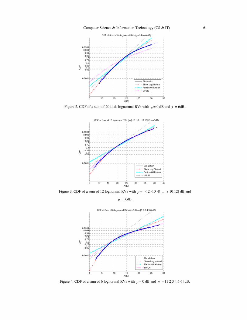
Computer Science & Information Technology (CS & IT) 61
5 10 15 20 25 30 35
0.0001
0.050.1
0.25
0.5
0.750.9
0.95
0.99
0.999
0.9999
X(dB)
CD
F
CDF of Sum of 20 lognormal RVs (µ=0dB,σ=6dB)
Simulation
Skew Log Normal
Fenton-Wilkinson
MPLN
Figure 2. CDF of a sum of 20 i.i.d. lognormal RVs with µ = 0 dB andσ = 6dB.
5 10 15 20 25 30 35 40 45
0.0001
0.050.1
0.25
0.5
0.750.9
0.95
0.99
0.999
0.9999
X(dB)
CD
F
CDF of Sum of 12 lognormal RVs (µ=[-12 -10 .. 10 12]dB,σ=6dB)
Simulation
Skew Log Normal
Fenton-Wilkinson
MPLN
Figure 3. CDF of a sum of 12 lognormal RVs with µ = [-12 -10 -8 ... 8 10 12] dB and
σ = 6dB.
0 5 10 15 20 25 30
0.0001
0.050.1
0.250.5
0.750.9
0.950.99
0.9990.9999
X(dB)
CD
F
CDF of Sum of 6 lognormal RVs (µ=0dB,σ=[1 2 3 4 5 6]dB)
Simulation
Skew Log Normal
Fenton-Wilkinson
MPLN
Figure 4. CDF of a sum of 6 lognormal RVs with µ = 0 dB and σ = [1 2 3 4 5 6] dB.

62 Computer Science & Information Technology (CS & IT)
5. APPLICATION: OUTAGE PROBABILITY IN LOGNORMAL SHADOWING
ENVIRONMENT
In this section, we provide an example for outage probability calculation in lognormal shadowing
environment based on log skew normal approximation.
We consider a homogeneous hexagonal network made of 18 rings around a central cell. Fig. 5
shows an example of such a network with the main parameters involved in the study: R, the cell
range (1 km), Rc, the half-distance between BS. We focus on a mobile station (MS) u and its
serving base station (BS),iBS , surrounded by M interfering BS
To evaluate the outage probability, the noise is usually ignored due to simplicity and negligible
amount. Only inter-cell interferences are considered. Assuming that all BS have identical
transmitting powers, the SINR at the u can be written in the following way:
, , ,
, , ,
0, 0,
.Y .Y
.Y .Y
i i u i u i i u
M M
j j u j u j j u
j j i j j i
PKr rSSINR
I NP Kr N r
η η
η η
− −
− −
= ≠ = ≠
= = =+
+∑ ∑ (30)
The path-loss model is characterized by parameters K and η >2. The term l lPKr
η− is the mean
value of the received power at distance lr from the transmitter lBS .Shadowing effect is
represented by lognormal random variable l,
10, 10
ux
l uY = where l,ux is a normal RV, with zero mean
and standard deviation σ, typically ranging from 3 to 12 dB.
Figure 5. Hexagonal network and main parameters
The outage probability is now defined as the probability for the γ SINR to be lower than a
threshold valueδ :

Computer Science & Information Technology (CS & IT) 63
,int
,
0,
,
,
0 ,
int,dB ,
.Y( ) ( ) ( )
.Y
.Y(10 log( ) )
.Y
( )
i i u
M
extj j u
j j i
i i u
dBM
j j u
j j i
ext dB dB
rPP P P
Pr
rP
r
P P P
η
η
η
η
γ δ δ δ
δ
ξδ
−
−
= ≠
−
−
= ≠
< = < = <
= <
= − <
∑
∑(31)
Where:
int,dB ,ln( .Y )i i u
P r η−= a normal RV with mean ln( )im r η−= and standard deviation ξσ .
ext,dB ,
0 ,
ln( .Y )M
j j u
j j i
P rη−
= ≠
= ∑ a skew normal RV with distribution ( , , )SN λ ε ω .
It is easy to show that the difference int,dB ,ext dB
P P− has a skew normal distribution 1 1 1( , , )SN λ ε ω
Where
1
2 2 2
1
12 2
2
2
m e
(1 )( ) 1
ε
ω ξ σ ω
λλ
ξ σλ
ω
= −
= +
=
+ +
Fig. 6 and Fig. 7 show the outage probability at cell edge (r=Rc) and inside the cell (r=Rc/2),
resp. for =3dB and 6dB assuming η=3. Difference between analysis and simulation results is less
than few tenths of dB. This accuracy confirms that the LSKN approximation considered in this
work is efficient for interference calculation process.
-20 -15 -10 -5 0 5 10 15 200
0.1
0.2
0.3
0.4
0.5
0.6
0.7
0.8
0.9
1Outage probability for a mobile located at r=Rc(a),Rc/2(b), σ=3dB
γ [dB]
Outa
ge p
robabili
ty
Simulation
LSKN Approximation
(b)
(a)
Figure 6. Outage probability for a mobile located at r=Rc (a), r=Rc /2(b), σ =3dB, η =3

64 Computer Science & Information Technology (CS & IT)
-20 -15 -10 -5 0 5 10 15 200
0.1
0.2
0.3
0.4
0.5
0.6
0.7
0.8
0.9
1Outage probability for a mobile located at r=Rc(a),Rc/2(b), σ=6dB
γ [dB]
Outa
ge p
robabili
ty
Simulation
LSKN Approximation
(b)(a)
Figure 7. Outage probability for a mobile located at r=Rc (a), r=Rc /2(b), σ =6dB, η =3
6. CONCLUSIONS
In this paper, we proposed a fitting method to log skew normal distribution in order to approximate the sum of lognormal distributions. The proposed fitting method uses moment and
tails slope matching technique to generate distribution parameters. By obtaining such parameters
through a simple procedure, the LSN random variable approximates the entire lognormal sum distribution with high accuracy, especially at the lower region. Simulations confirm that our
fitting method outperforms other priori methods for all cases except for the case when lognormal
distributions have different standard deviation. Using an example for outage probability
calculation in lognormal shadowing environment, we proved that LSKN approximation,
considered in this work, is efficient for interference calculation process.
Appendix A
We begin by showing that the LSKN distribution has a best lognormal fit [27] at the right tail.
Using [22, Lemma 1], for a given λ > 0
,
,
,
1 (x)lim
ln(x)1 ( )
1 (x)lim
x1 ( )
xlim (1 (x)) 2
(x)
LSKN
x
SKN
x
SKNx
F
w
F
w
F
λ
λ
λ
εφ
εφ
ϕ
→+∞
→+∞
→+∞
−
−−
−=
−−
= − =
Because this ratio converges to a finite non–zero value, we may conclude from [21, Lemma 2]
that x( )
w
εφ
− is a best lognormal fit to SKLN
F at the right tail. The corresponding slope is 1/ ω on
lognormal paper, which proves (25)
In order to prove the lower tail slope, a few steps are needed. Using [22, Lemma 1], for a given
λ > 0 we have:

Computer Science & Information Technology (CS & IT) 65
2 2
,
,
,
2
2 2
(1 )
2
2 2
lim ( )
lim (1 ( ))
lim (1 ( ))
2 ( 1 )lim
(1 )
elim
(1 )
SKNx
SKNx
SKNx
x
x
x
F x
F x
F x
x
x
x
λ
λ
λ
λ
ϕ λ
π λ λ
πλ λ
→−∞
−→−∞
−→+∞
→+∞
+−
→+∞
= − −
= −
+=
+
=+
Using approximation from [25]:
012ln(2 ) ln( ln(2 ))
xx xφ π
+→− →− − − −
After some manipulation, we may write:
Which proves (26).
REFERENCES
[1] J. M. Kelif , M. Coupechoux and P. Godlewski "On the dimensioning of cellular OFDMA networks",
Phys. Commun., vol. 5, no. 1, pp.10 -21 2012.
[2] L. F. Fenton,“The sum of log-normal probability distributions in scatter transmission systems”, IRE
Trans. Commun., Vol. 8, pp.57-67, March 1960.
[3] N. Beaulieu and Q. Xie, “An optimal lognormal approximation to lognormal sum distributions,” IEEE
Trans. Vehicular Tech., vol. 53, pp. 479–489, Mar. 2004.
[4] J. Wu, N. B. Mehta, J. Zhang, “Flexible lognormal sum approximation method,” IEEE GLOBECOM
2005, vol. 6, Nov. 2005, pp. 3413–3417.
[5] Z. Liu, J. Almhana, F. Wang, and R. McGorman, "Mixture lognormal approximations to lognormal
sum distributions," IEEE Commun. Lett., vol. 11, pp. 711-713, Sept. 2007.
[6] N. C. Beaulieu, Q. Xie, “Minimax Approximation to Lognormal Sum Distributions”, IEEE VTC
Spring, Vol. 2, pp. 1061-1065, April 2003.
[7] Tellambura, C., Senaratne, D.,“Accurate computation of the MGF of the lognormal distribution and
its application to sum of lognormals”, Communications, IEEE Transactions on, Vol. 58, No. 5, pp.
1568-1577, May 2010.
[8] Damith Senaratne, Chintha Tellambura: Numerical Computation of the Lognormal Sum Distribution.
GLOBECOM, page 1-6. IEEE, 2009.
[9] N. C. Beaulieu "Fast convenient numerical computation of lognormal characteristic functions", IEEE
Trans. Commun., vol. 56, no. 3, pp.331 -332 2008.

66 Computer Science & Information Technology (CS & IT)
[10] Mahmoud, A.S.H. "New Quadrature-Based Approximations for the Characteristic Function and the
Distribution Function of Sums of Lognormal Random Variables", Vehicular Technology, IEEE
Transactions on, On page(s): 3364 - 3372 Volume: 59, Issue: 7, Sept. 2010.
[11] H. Nie and S. Chen, "Lognormal sum approximation with type IV Pearson distribution," IEEE
Commun. Lett., vol. 11, no. 10, pp. 790-792, Oct. 2007.
[12] M. Di Renzo , F. Graziosi and F. Santucci "Further results on the approximation of lognormal power
sum via Pearson type IV distribution: a general formula for log moments computation", IEEE Trans.
Commun., vol. 57, pp.893 -898 2009.
[13] N. C. Beaulieu, F. Rajwani, “Highly accurate simple closed-form approximations to lognormal sum
distributions and densities,” IEEE Communications Letters, vol.8, Dec. 2004, pp. 709–711.
[14] C. L. J. Lam and T. Le-Ngoc "Estimation of typical sum of lognormal random variables using log
shifted gamma approximation", IEEE Commun. Lett., vol. 10, no. 4, pp.234 -235 2006.
[15] Z. Liu, J. Almhana, and R. McGorman, “Approximating lognormal sum distributions with power
lognormal distributions,” IEEE Trans. Vehic. Tech., vol. 57, pp. 2611–2617, July 2008.
[16] Szyszkowicz, S.S, Yanikomeroglu, H, “Fitting the Modified–Power–Lognormal to the Sum of
Independent Lognormals Distribution”, Global Telecommunications Conference, 2009.
GLOBECOM 2009.
[17] S. S. Szyszkowicz and H. Yanikomeroglu "On the tails of the distribution of the sum of lognormals",
Proc. IEEE International Conf. Commun. (ICC), pp.5324 -5329, 2007.
[18] Z. Wu, X. Li, R. Husnay, V. Chakravarthy, B. Wang, and Z. Wu. A novel highly accurate log skew
normal approximation method to lognormal sum distributions. In Proc. of IEEE WCNC 2009.
[19] X. Li, Z. Wu, V. D. Chakravarthy, and Z. Wu, "A low complexity approximation to lognormal sum
distributions via transformed log skew normal distribution," IEEE Transactions on Vehicular
Technology, vol. 60, pp. 4040-4045, Oct. 2011.
[20] S. Asmussen and L. Rojas-Nandayapa, “Asymptotics of sums of lognormal random variables with
Gaussian copula,” Statistics & Probability Letters, vol. 78, pp. 2709–2714, Nov. 2008.
[21] S. Szyszkowicz and H. Yanikomeroglu, “On the tails of the distribution of the sum of lognormals,”
IEEE ICC, pp. 5324–5329, June 2007.
[22] Archil Gulisashvili, Peter Tankov, “Tail behavior of sums and differences of log-normal random
variables”, ARXIV 09/2013
[23] Antonella Capitanio, “On the approximation of the tail probability of the scalar skew-normal
distribution”, in METRON (2010)
[24] W. Hürlimann, “Tail Approximation of the Skew-Normal by the Skew-Normal Laplace: Application
to Owen’s T Function and the Bivariate Normal Distribution”, Journal of Statistical and Econometric
Methods, vol. 2, no.1, 2013, 1-12, Scienpress Ltd, 2013
[25] H. E. Fettis, “A stable algorithm for computing the inverse error function in the “tail-end” region,”
Mathematics of Computation, vol. 28, pp. 585–587, Apr. 1974.
[26] O’Hagan A. and Leonard TBayes estimation subject to uncertainty about parameter constraints,
Biometrika, 63, 201–202, 1976.
[27] Azzalini A, A class of distributions which includes the normal ones, Scand. J. Statist., 12, 171–178,
1985.
AUTHORS
Marwane Ben Hcine was born in Kébili, Tunisia, on January 02, 1985. He
graduated in Telecommunications Engineering, from The Tunisian Polytechnic
School (TPS), July 2008. In June 2010, he received the master’s degree of research
in communication systems of the Higher School of Communication of Tunisia
(Sup’Com). Currently he is a Ph.D. student at the Higher School of
Communication of Tunisia. His research interests are network design and
dimensioning for LTE and beyond Technologies.

Computer Science & Information Technology (CS & IT) 67
Pr. Ridha BOUALLEGUE was born in Tunis, Tunisia. He received the M.S degree
in Telecommunications in 1990, the Ph.D. degree in telecommunications in 1994, and
the HDR degree in Telecommunications in 2003, all from National School of
engineering of Tunis (ENIT), Tunisia. Director and founder of National Engineering
School of Sousse in 2005. Director of the School of Technology and Computer Science
in 2010. Currently, Prof. Ridha Bouallegue is the director of Innovation of
COMmunicant and COoperative Mobiles Laboratory, INNOV’COM Sup’COM,
Higher School of Communication. His current research interests include mobile and cooperative
communications, Access technique, intelligent signal processing, CDMA, MIMO, OFDM and UWB
systems.

68 Computer Science & Information Technology (CS & IT)
INTENTIONAL BLANK

Natarajan Meghanathan et al. (Eds) : NeTCoM, CSIT, GRAPH-HOC, SPTM - 2014
pp. 69–77, 2014. © CS & IT-CSCP 2014 DOI : 10.5121/csit.2014.41306
SELECTIVE IMAGE ENCRYPTION USING
DCT WITH AES CIPHER
Belazi Akram, Benrhouma Oussama, Hermassi Houcemeddine and
Belghith Safya
SysComLab, Ecole Nationale d’Ingénieurs de Tunis (ENIT), Tunis, Tunisia [email protected]
ABSTRACT
Selective encryption presents a great solution to optimize time efficiency during encryption
process. In this paper a novel selective encryption scheme based on DCT transform with AES
algorithm is presented. In the DCT method, the basic idea is to decompose the image into 8×8
blocks and these blocks are transformed from the spatial domain to the frequency domain by the
DCT. Then, the DCT coefficients correlated to the lower frequencies of the image block are
encrypted. The proposed cryptosystem is evaluated using various security and statistical
analysis; results show that the proposed algorithm is strong against attacks and suitable for
practical application.
KEYWORDS
DCT, Selective Encryption, AES Cipher
1. INTRODUCTION
Nowadays, multimedia content (image, audio and video) presents an enormous importance giving
the fact of the rapid growth of high technologies. The rate of exchanges these types of
information is growing and the need to protect it is more and more essential. However increasing
number of digital documents, multimedia processing tools, and the worldwide availability of
Internet access has created an ideal way to uncontrollable distribution of multimedia content [1].
To protect data, various encryption schemes has been proposed for image encryption, [2,3,4]
however in these schemes (total encryption schemes) all data has to be encrypted which will
generally take some time, complicated calculations and high memory occupation, which makes
these schemes hard to use in real time applications.
Total encryption schemes are not necessary when we talking about most multimedia content.
Given to the fact that the content is already voluminous and not all the content represents a
significant importance we choose to encrypt only significant parts of the data and leave the rest to
enhance time encryption and reduce memory occupation and make the encryption scheme
suitable in practical application given to the fact that selective crypto-systems presents a simple
architecture.
Selective encryption protects the most visually important parts of an image or video
representation [5,6,7]. Encrypting only parts of the image data must be sufficient to satisfy the
needed security [8,9]. There are two basic ways to encrypt digital images: in the spatial domain or
in the transform domain [10]. Since wavelet based compression appeared and was adopted in the

70 Computer Science & Information Technology (CS & IT)
JPEG2000 standard, suggestions for image encryption techniques based in the wavelet domain
have been abundant. However, many of these are not secure as they are based exclusively on
random permutations making them vulnerable to known or chosen-plaintext attacks [11, 12, 13,
19]. For example, in DCT codec several selective encryption schemes have been proposed.
Droogenbroeck and Benedett [14] selected AC coefficients from compressed images for
encryption. In their method the DC coefficients are not ciphered because they carry important
visible information and they are highly predictable. The compression and encryption operations
are separated in this approach and this requires an additional operating cost. Jiang-Lung Liu [15]
proposes to encrypt the low-frequency DCT coefficients only and leave the high-frequency ones
unencrypted in the JPEG compression.
In this paper we propose a selective encryption scheme based on DCT transformation and AES
algorithm to cipher digital images.
The rest of the paper is organized as follow: section 2 presents a mathematical preliminary for the
DCT transform, section 3 we present our encryption, experimental results are presented in section
and we conclude in section 5.
2. FREQUENCY BAND ENCRYPTION IN A DCT BLOCK
In a DCT-based codec, media data are partitioned into blocks (typically, 8 × 8 or 4 × 4), and each
block is transformed by DCT, quantized and encoded with entropy coding. Generally, the DCT
block is scanned in zigzag order, which generates the coefficient sequence ordered from the
highest frequency to the lowest frequency. In this coefficient sequence, the first coefficient
denotes the DCT block’s energy, and the other coefficients denote detailed information on the
image block. The DCT block is scanned from the bottom- left to the top- right, as shown in
Figure 1. Thus, the first coefficient in the coefficient sequence denotes the block’s energy.
In perceptual encryption, the 64 coefficients can be selected from the first one to the last one
according to the quality factor Q. Thus, set N = 64 for each DCT block. Figure 2 shows the
relation between n and the PSNRs of the encrypted images. As can be seen, with increase in n, the
quality of the images decreases.
Figure 1. Coefficient sequence generation in a DCT block
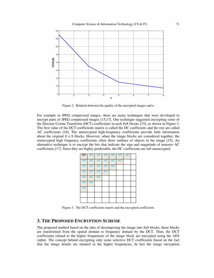
Computer Science & Information Technology (CS & IT) 71
Figure 2. Relation between the quality of the encrypted images and n
For example in JPEG compressed images, there are many techniques that were developed to
encrypt parts of JPEG compressed images [15,17]. One technique suggested encrypting some of
the Discrete Cosine Transform (DCT) coefficients in each 8x8 blocks [15], as shown in Figure 3.
The first value of the DCT coefficients matrix is called the DC coefficient, and the rest are called
AC coefficients [16]. The unencrypted high-frequency coefficients provide little information
about the original 8 x 8 blocks. However, when the image blocks are considered together, the
unencrypted high frequency coefficients often show outlines of objects in the image [15]. An
alternative technique is to encrypt the bits that indicate the sign and magnitude of nonzero AC
coefficients [17]. Since they are highly predictable, the DC coefficients are left unencrypted.
Figure 3. The DCT coefficients matrix and the encrypted coefficients
3. THE PROPOSED ENCRYPTION SCHEME
The proposed method based on the idea of decomposing the image into 8x8 blocks, these blocks
are transformed from the spatial domain to frequency domain by the DCT. Then, the DCT
coefficients related to the higher frequencies of the image block are encrypted using the AES
cipher. The concept behind encrypting only some selective DCT coefficients based on the fact
that the image details are situated in the higher frequencies, In fact the image encryption

72 Computer Science & Information Technology (CS & IT)
algorithm obtains higher security when DCT coefficients related to the lower frequencies are
encrypted than those related to higher frequencies. Fig. 4 shows the general block diagram of the
proposed method of selective image encryption. We propose a secure encryption scheme:
(i) Block 1: All coefficients are encrypted.
(ii) Blocks 2, 3. . . n: The 24 most significant bit-planes are encrypted.
Where n is the number of block.
The general block diagram of the proposed method of selective image encryption is shown in
Figure 4, which combines encryption process with DCT codec, and is composed of data
encoding, parameter encryption and data decoding. Here, P, K and C are the plaintext, key and
ciphertext, respectively. X and Y are the parameters in the data stream, among which, X is
encrypted into Z according to Z = E(X, K) while Y is left unchanged. Without losing the
generality, the data stream composed of two parameters is investigated. If the data steam is
composed of more parameters, the similar results can be obtained.
4. EXPERIMENTAL RESULTS
In this section, the performance of the proposed image encryption scheme is analyzed in detail. It
is well known that statistical analysis is of crucial importance. Indeed, an ideal cipher should be
robust against any statistical attack. In order to prove the robustness of proposed image
encryption scheme, we have performed some statistical tests which are described in the following.
Figure 4. Block diagram of the proposed method
4.1. Histogram
To demonstrate that our proposed algorithm has strong resistance to statistical attacks, test is
carried out on the histogram of enciphered image. Several gray-scale images of size 256×256 are
selected for this purpose and their histograms are compared with their corresponding ciphered
image. One typical example is shown below. The histogram of the original image contains large
spikes as shown in Figure 5 but the histogram of the ciphered image as shown in Figure 6, is
more uniform. It is clear that the histogram of the encrypted image is, significantly different from
the respective histogram of the original image and bears no statistical resemblance to the plain
image. Hence statistical attack on the proposed image encryption procedure is difficult.

Computer Science & Information Technology (CS & IT) 73
Figure 5. Histogram of Original Image
Figure 6. Histogram of Encrypted Image
4.2. Correlation of adjacent pixels
It is well known that adjacent image pixels are highly correlated either in horizontal, vertical or
diagonal directions. Such high correlation property can be quantified by means of correlation
coefficients which are given by:
Where,
qi and pi denote two adjacent pixels (either horizontal or vertical). S is the total number of duplets
(pi,qi) obtained from the image; and are the mean values of pi and qi , respectively. The
correlation coefficients of the plain and ciphered images of Lena and Boat are given in the Table
1. It can be observed that the encrypted images obtained from the proposed scheme have small
correlation coefficients in horizontal, vertical and diagonal directions. The result are illustrated in
Figure 7 and Figure 8, which presents the distribution of two adjacent pixels in the original and
encrypted images of Lena and Boat for horizontal (a-b), vertical (c-d) and diagonal (e-f)
directions.
)1()()(
),cov(
qDpD
qpr =
∑=
−=
S
i
i ppS
pD1
2)(
1)(
))((1
),cov(1
qqppS
qp i
S
i
i −−= ∑=

74 Computer Science & Information Technology (CS & IT)
Figure 7. the distribution of two adjacent pixels in the original and encrypted lena.
Figure 8. the distribution of two adjacent pixels in the original and encrypted boat.
Table 1. Correlation coefficients of two adjacent pixels in original and encrypted images.
Image Horizontal Vertical Diagonal
Original Encrypted Original Encrypted Original Encrypted
Lena 0.9888 0.0138 0.9917 -0.0383 0.9923 0.0171
Boat 0.9829 -0.0016 0.9818 -0.0682 0.9769 -0.1169
4.3. Differential attack
As a general requirement for all the image encryption schemes, the encrypted image should be
greatly different from its original form. Such difference can be measured by means of two criteria
namely, the NPCR (Number of Pixel Change Rate) and the UACI (Unied Average Changing
Intensity) [18]. The NPCR is used to measure the number of pixels in difference between two
images. Let S(i,j) and S’(i,j) be the (i,j)th pixel of two images S and S’ ,respectively.
The NPCR can be defined as:
)2(%100
),(;
×=
∑
L
jiD
NPCRji

Computer Science & Information Technology (CS & IT) 75
Where L is the total number of pixels in the image and D(i,j) is defined as :
Where S(i,j) and S’(i,j) are the pixel values of the two images, respectively. For instance, for two
random images:
The second criterion, UACI, is used to measure the average intensity difference and can be
defined as:
Where B is the number of bits used to represent a grey scale pixel value. In the case of two
random images, the expected value of UACI is:
The NPCR and UACI measured between the plain and ciphered images of Lena and Boat with
the proposed cryptosystem are given in Table 2.
Table 2. Sensitivity to differential attacks.
Image NPCR% UACI%
Lena 99.5941 33.7715
Boat 99.5895 33.4626
4.4. Information entropy
Entropy is a statistical measure of randomness. Ideally, the information entropy should be 8 bits
for gray scale images. Table 3 shows the entropy of different test images of size 256×256.
Table 3. Entropy results for encrypted images.
It’s seen that the value of entropy for encrypted images is very close to the 8 bits, then the loss of
information is negligible, and the proposed algorithm is strong against entropy attack.
5. CONCLUSIONS
Selective Image Encryption Using DCT with AES Cipher has been presented in this paper. The
algorithm will not encrypt bit by bit the whole image but only selective DCT coefficients will be
encrypted. Indeed the proposed encryption method uses the Selective Encryption approach where
the DC coefficients and some selective AC coefficients are encrypted, hence the DC coefficients
carry important visual information, and it's difficult to predict the selective AC coefficients, this
give a high level of security in comparison with methods mentioned above. Several security and
Image Entropy of Encrypted Image
Lena 7.8683
Boat 7.8745
≠
=
),('),(1
),('),(0),(
jiSjiSif
jiSjiSifjiD
%609375.99=NPCR
)3(%10012
),('),((
1×
−
−
= ∑ B
jiSjiS
LUACI
%46354.33=UACI

76 Computer Science & Information Technology (CS & IT)
statistical analysis tests are carried out in order to check the robustness of the proposed algorithm.
Both simulations and analysis results prove the efficiency of the proposed cryptosystem.
REFERENCES
[1] IEEE Transactions on Circuits and Systems for Video Technology (2003) : Special Issue on
Authentication, Copyright Protection, and Information Hiding, Vol. 13, No. 8.
[2] Liansheng Sui, Kuaikuai Duan, Junli Liang, Zhiqiang Zhang & Haining Meng , (2014) Asymmetric
multiple-image encryption based on coupled logistic maps in fractional Fourier transform domain”,
Optics and Lasers in Engineering, Volume 62, Pages 139-152
[3] A. Alfalou, C. Brosseau & N. Abdallah, (2015) “Simultaneous compression and encryption of color
video images”, Optics Communications, Volume 338, Pages 371-379
[4] Tieyu Zhao, Qiwen Ran & Yingying Chi, (2015) “Image encryption based on nonlinear encryption
system and public-key cryptography”, Optics Communications, Volume 338, Pages 64-72
[5] Li-feng WANG, Wen-dong WANG, Jian MA, Chen XIAO & Kong-qiao WANG, (2008) “Perceptual
video encryption scheme for mobile application based on H.264”, The Journal of China Universities
of Posts and Telecommunications, Volume 15, Supplement, Pages 73-78.
[6] Sukalyan Som & Sayani Sen, (2013) “A Non-adaptive Partial Encryption of Grayscale Images based
on Chaos”, Procedia Technology, Volume 10, Pages 663-671.
[7] Xinjun Zhang & Xingyuan Wang, (2013) “Chaos-based partial encryption of SPIHT coded color
images”, Signal Processing, Volume 93, Pages 2422-2431.
[8] Nidhi Taneja, Balasubramanian Raman & Indra Gupta, (2011) “Selective image encryption in
fractional wavelet domain”, AEU - International Journal of Electronics and Communications, Volume
65, Issue 4, Pages 338-344.
[9] Gaurav Bhatnagar & Q.M. Jonathan Wu, (2012) “Selective image encryption based on pixels of
interest and singular value decomposition”, Digital Signal Processing, Volume 22, Issue 4, July 2012,
Pages 648-663.
[10] S. Li & G. Chen, (2004) “Chaos-Based Encryption for Digital Images and Videos”, in Multimedia
Security Handbook, B. Furht and D. Kirovski, CRC Press.
[11] Akram Belazi, Houcemeddine Hermassi, Rhouma Rhouma & Safya Belghith, (2014) “Algebraic
analysis of a RGB image encryption algorithm based on DNA encoding and chaotic map”, Nonlinear
Dynamics June, Volume 76, Issue 4, pp 1989-2004.
[12] Houcemeddine Hermassi, Akram Belazi, Rhouma Rhouma & Safya Mdimegh Belghith, (2014)
“Security analysis of an image encryption algorithm based on a DNA addition combining with chaotic
maps”, Multimedia Tools and Applications ,Volume 72, Issue 3, pp 2211-2224.
[13] Rhouma Rhouma, Ercan Solak & Safya Belghith, (2010) “Cryptanalysis of a new substitution–
diffusion based image cipher, Communications in Nonlinear Science and Numerical Simulation,
Volume 15, Issue 7, Pages 1887-1892.
[14] M. Van Droogenbroeck & R. Benedett, (2002) “Techniques for a Selective Encryption of
Uncompressed and Compressed Images”, in Proceedings of Advanced Concepts for Intelligent Vision
Systems (ACIVS) 2002, Ghent, Belgium.
[15] Jiang-Lung Liu (2006) “Efficient selective encryption for JPEG 2000 images using private initial
table”. Pattern Recognition, Volume 39, Issue 8, Pages 1509-1517.
[16] K. Sayood, (2000) “Introduction to Data Compression”, 2nd edition, USA, Morgan Kauffman
Publishers.
[17] Saeed Bahrami & Majid Naderi, (2013) “Encryption of multimedia content in partial encryption
scheme of DCT transform coefficients using a lightweight stream algorithm”, Optik - International
Journal for Light and Electron Optics, Volume 124, Issue 18, Pages 3693-3700.
[18] G. Chen, Y. Mao, & C. K Chui, (2004) “A symmetric image encryption based on 3D chaotic maps,”
Chaos Soliton Fractals, vol. 21, pp. 749–761.
[19] Oussama Benrhouma •Houcemeddine Hermassi & Safya Belghith, (2013) “Security analysis and
improvement of a partial encryption scheme,” Multimedia Tools and Applications DOI
10.1007/s11042-013-1790-4.

Computer Science & Information Technology (CS & IT) 77
AUTHORS
Akram BELAZI has received his engineering diplomat in “Telecommunication &
Networks” in 2011 at the National Engineering School of Gabes, ENIG Tunisia and his
Master degree in “Electronic Systems and Networks Communications” in 2013 at the
Polytechnic School of Tunisia, EPT. He is now a Phd student at the Syscom Laboratry,
ENIT Tunisia. His researcher domain is focused on the conception of partial encryption
scheme for multimedia content and cryptanalysis of chaos-based cryptosystem
Oussama Benrhouma is a PhD student in the Syscom laboratory at the ENIT Ecole
Nationale d’Ingénieurs de Tunis (ENIT). His domain of interest includes cryptography,
Multimedia watermarking and steganography.
Houcemeddine Hermassi has received his engineering diploma in “Telecommunications
& Networks” in 2005 from the National School of Engineering Gabès ENIG, Tunisia, and
his MS degree in “Communication Systems” in 2010 from the National School of
Engineering Tunis ENIT, Tunisia. He is now a PhD student at the Syscom Laboratory,
ENIT Tunisia. His researcher domain is focused on the cryptanalysis and the conception
of the new multimedia cryptographic approaches like the chaos-based cryptography and
the DNA cryptography.
Prof. Safya Belghith has received his engineering diploma in “Electricity” (1981) and
his D.E.A (1982) and the PhD degree (1985) in “Automatic and Signal Processing” from
the High School of Electricity, Lab Signals & Systems, University Paris XI Orsay. In
1997, she received her Status Doctorate in “Physical Sciences” from the Faculty of
Sciences Tunis FST with collaboration of the Laboratory Signals & Systems, High
School of Electricity University Paris XI Orsay. She is now a Professor at the National
School of Engineering Tunis ENIT, Tunisia and a senior researcher at SysCom Laboratory in the ENIT,
Tunisia. His research domain is focused on the analysis of nonlinear systems and chaotic communication,
the generation of the pseudo random sequences from chaotic systems and studying their performance in
mobile radio communications particularly in a DS/CDMA and on the Synchronization of chaotic systems
and its application to secure the transmission by chaotic carrier – Cryptography.

78 Computer Science & Information Technology (CS & IT)
INTENTIONAL BLANK

Natarajan Meghanathan et al. (Eds) : NeTCoM, CSIT, GRAPH-HOC, SPTM - 2014 pp. 79–96, 2014. © CS & IT-CSCP 2014 DOI : 10.5121/csit.2014.41307
DYNAMIC OPTIMIZATION OF OVERLAP-
AND-ADD LENGTH OVER MBOFDM
SYSTEM BASED ON SNR AND CIR
ESTIMATE
Nouri Naziha and Bouallegue Ridha
Innov’Com Laboratory, Higher School of Communications of Tunis, Sup'Com, University 7th November at Carthage, Tunisia.
ABSTRACT
An important role performed by Zero Padding (ZP) in multi-band OFDM (MB-OFDM) System.
This role show for low-complexity in résistance against multipath interference by reducing
inter-carrier interference (ICI) and eliminating the inter-symbol interference (ISI) Also, zero-
padded suffix can be used to eliminate ripples in the power spectral density in order to conform
to FCC requirements.
At the receiver of MB-OFDM system needs to use of a technique called as overlap-and-add
(OLA). Which maintain the circular convolution property and take the multipath energy of the
channel.
In this paper, we proposed a method of performing overlap-and-add length for zero padded
suffixes. Then, we studied the effect of this method, dynamic optimization of overlap-and-add
(OLA) equalization, on the performance of MBOFDM system on Bit Error Rate (BER) with
AWGN channel and Saleh-Valenzuela (S-V) Multipath channel Model.
In the dynamic optimization OLA, the Length of ZP depends on length of channel impulse
response (CIR). These measures, based on SNR, insert the ZP according to the measurement.
Dynamic optimization of length of ZP improves the Performance of MBOFDM system. In fact
we developed a technique to select the length of ZP as function of SNR and CIR
estimate(repetition). In our simulation this technique improve to 3 dB at BER=10-2
with a
multipath channels CM4.
KEYWORDS
UWB, ECMA-368, MB-OFDM, OLA, ZPS, SNR, CIR, BER.

80 Computer Science & Information Technology (CS & IT)
1. INTRODUCTION
Ultra-wideband (UWB) has tremendous potential for high-rate [1] low-power communication due to its high data rates and resistance to interference. Since its lowly beginning in the decade of 1940, UWB technology has traveled a wealthy path, from lab to military, back to lab [2] and this technology has received significant attention from industry, media and academia [3] especially in wireless universal serial bus (WUSB) and wireless personal area network (WPAN) domain [2]. The reason for all this excitement is that this technology promises to deliver high data rates that can scale from 110 Mbit/s at a distance of 10 meters up to 480 Mbit/s at a distance of two meters in realistic multipath environments all while consuming very little power communication and resistance to interference [1]. It is expected that UWB devices will provide low cost solutions [3].The United States Federal communications commission (FCC) officially defined UWB in 2002 as a signal with a 10 dB bandwidth of at least 500 MHz and a maximum equivalent isotropic radiated power spectral density (PSD) of no more than -41.3 dBm/MHz in the 3.1-10.6 GHz band [4]. FCC ruled that UWB system must have instantaneous spectrum of more than 500 MHz or more than 20% of its central frequency [2]. In order that UWB systems appear in the thermal noise floor of the existing narrowband services like GSM, GPS etc., and coexist with them without affecting their performance [5][6].Efficient utilization of such a large bandwidth of 7.5 GHz creates a huge challenge to the system designer community [2]. Furthermore the power constraints limits the range of communication to a short range only around 2 m to 15 m with scalable data rate of 53.3 Mbps to 480 Mbps. A promising new high-speed wireless communication technology, called Multiband-Orthogonal Frequency Division Multiplexing (MB-OFDM) approach, designers can overcome many of barriers [3] such as complexity, cost, power consumption, and flexibility. Pulsed multiband technique presented many disadvantages that can overcome if we use symbol which is much longer in time domain and integrating a modulation technique that can efficiently capture multipath energy [2]. MB-OFDM approach is the right candidate for this choice [7]. The main advantage of this approach is that information is processed over a much smaller bandwidth, this approach can reduce the system design complexity, the power consumption, cost, and also improving spectral flexibility which in turn helps UWB systems to follow global compliance [2][3]. Other advantages of this scheme include using lower-rate ADCs and simplifying the digital complexity. Systems built using this type of approach are often referred to as multiband systems [3]. The MB-OFDM is the first UWB technology obtained international standardization Thanks to their multiple benefits [8],[9] developed by the WiMedia alliance. Also this technology has been enabled by the FCC's recent allocation of 7500MHz. The MB-OFDM support data from 53.3 Mb/s to 480 Mb/s and divides the several gigahertz of spectrum allocated by the FCC into 14 bands, each with 528 MHz bandwidth. These bands are then bundled into 5 band groups with only the first defined as mandatory [10]. ECMA-368 is one of such principal standard employing MB-OFDM technique [11]. MB-OFDM based UWB system takes all the positives offered by the multi-banding scheme such as low power, low cost, simple analog design and also is capable of capturing sufficient multipath energy using a single RF chain due to adopted OFDM scheme [2].

Computer Science & Information Technology (CS & IT) 81
Multicarrier schemes are supported to high data rate. OFDM is an attractive air-interface for next-generation wireless network without complex equalizer. OFDM is an emerging multi-carrier modulation scheme. It has been adopted by several wireless standards such as IEEE 802.11a, IEEE 802.16 and HiperLAN2. OFDM is designed such a way that it sends data over hundreds of parallel carrier which increases data rate. OFDM distributes data across a large number of carries that are spaced apart at accurate frequencies is modulated by the data. The Orthogonal FDM (OFDM) reaps its own advantage to this approach [12], [13] in terms of spectral efficiency, narrow band interference (NBI) mitigation, excellent robustness against multipath channel, and smoothing the use of low complexity equalizer in receiver [2]. OFDM scheme suffered from inter-symbol interference (ISI) problem. ISI is distortion in a signal in which one symbol interferes with subsequent symbols, this will degrade performance of OFDM system. There are several methods for reducing the effects of ISI by affording time for reflection multipath energy mitigation and to allow a transmitter and a receiver for switching between different frequency bands. A receiving device can use an operation called overlap and add to restore the orthogonality. There are diversities of techniques to represent the noise at the receiver. Characteristically, more noise that affects the modulated signals, this noise can be measure with the distance error between the received signal and the ideal symbol associated with them. When the distance error is greater more difficult it becomes to map received signal to their associated ideal symbol and may prevent the communication to occur in some cases. Thus, the problem of relatively overly noise being added during overlap-and-add operation is very important issue that must be addressed with solutions that overcome the deficiencies of the prior technique. In this paper, we proposed a dynamic optimization of length of ZP technique based on SNR and CIR estimate, in addition, we evaluate its effects on performance of MB-OFDM system. Section II present a brief description of the main component of MB-OFDM system, especially by using Zero-Pad OFDM Signal and Overlap and adds operation over AWGN Channel and the SV/ IEEE 802.15.3a Channel Model. A dynamic overlap and add length technique based on SNR and CIR estimate is provided in Section III. In particular, we proposed our process of computing dynamic OLA size based on SNR and CIR estimation. Simulation Results are discussed in Section IV with four different channel models (CM) defined by the IEEE 802.15.3a. Finally, we conclude with a summary of this work given in Section V.
2. SYSTEM MODEL 2.1. MB-OFDM System
MB-OFDM is the primary applicant for high data rate UWB applications. Today, this approach is supported by the WiMedia Alliance and adopted by the ECMA-368 standard. Our system is presented in Figure 1. The MB-OFDM solution consists in combining OFDM with a multiband technique. That divides the available spectrum into 14 sub-bands of 528 MHz each, as presented in Figure 2. The modulation OFDM with 128 subcarriers is applied separately on each sub-band. As illustrate in

82 Computer Science & Information Technology (CS & IT)
the Figure 2, these sub-bands are combined to form several groups. Each group from the four groups contains three subbands and the five group contain only two subbands. This division has the advantage of reducing the complexity and hence the costs of components including converters. A WiMedia compatible device should actually only use the first group (3.1 - 4.6GHz).
Table 1. Characteristics a MB-OFDM symbol
Parameter Description value
fs Sampling frequency 528 MHZ NFFT Total number of subcarriers (FFT size) 128 ND Number of data subcarriers 100 NP Number of pilot subcarriers 12 NG Number of guard subcarriers 10 NT Total number of subcarriers used 122(=ND+NP+NG) Df Subcarries frequency spacing 4.125 MHZ (=fs/NFFT)
TFFT IFFT and FFT period 242.42 ns (�f-1)
NZPS Number of samples in zero-padded suffix 37 TZPS Zero-padded suffix duration in time 70.08 ns(=NZPS/fs) TSYM Symbol interval 312.5 ns (=TFFT + TZPS) FSYM Symbol rate 3.2 MHZ (=TSYM
-1) NSYM Total number of samples per symbol 165(=NFFT + NP)
The characteristics of the OFDM symbols, used in the MBOFDM system, are listed in Table 2. The OFDM symbols are generated by a 128 point IFFT. Which 100 are dedicated to user data, 12 and 10 pilot to data guards. The inter-carrier interval �f=4.125 MHz can satisfy the orthogonality condition of the OFDM multiplex. The duration of the suffix zero-padding is Tzps = 70.08 ns, 37 samples. Only the first 32 samples are devoted to the guard interval is a period TZP = 60.61 ns. The last 9.47 ns themselves being used to effect the change of central frequency of OFDM symbols. Each OFDM symbol transmitted has a duration Ts = 312.5 ns and therefore includes 165 samples. The MB-OFDM system, which presented in Figure 1, uses three sub-bands of the group, to which is applied a frequency hopping called time-frequency code (TFC). The TFC is used to control frequency hopping between different subbands. Moreover this method specifies for each OFDM symbol its central transmission frequency. Thus, as shown in Figure 2, each symbol has a different subband of the preceding symbol.
Figure 1. MBOFDM system

Computer Science & Information Technology (CS & IT) 83
Figure 2. Example of time-frequency coding for MB-OFDM systems in the group1, TFC = {1,2,3,1,2,3,...}
Furthermore the MB-OFDM system transmits information at different data rates varying from 53.3 to 480 Mbps, listed in Table1. These data rates are established by the use of different convolutional coding rates and puncturing technique. As well this system include bit interleaving, constellation mapping QPSK/DCM, frequency-domain spreading (FDS) and time-domain spreading (TDS) techniques. To retrieve the data, a receiver can put technical implementation as removing ZP overlap and add, channel estimation, equalization, de-spread, de-mapping, de-interleaving, de-puncture, de-coding.
Table 2. WiMedia-based MB-OFDM data rates
Figure 3. UWB spectrum bands in the MB-OFDM solution
Data Rate
(MB/s)
Modulation Code Rate (R) FDS TDS Coded Bits/6
OFDM Symbol
(NCBP6S)
Info Bits/6
OFDM Symbol
(NIB6S)
53.3 QPSK 1/3 YES YES 300 100 80 QPSK 1/2 YES YES 300 150
106.7 QPSK 1/3 NO YES 600 200 160 QPSK 1/2 NO YES 600 300 200 QPSK 5/8 NO YES 600 375 320 DCM 1/2 NO NO 1 200 600 400 DCM 5/8 NO NO 1 200 750 480 DCM 3/4 NO NO 1 200 900

84 Computer Science & Information Technology (CS & IT)
2.2. The SV/ IEEE 802.15.3a Channel Model Since UWB channels take a some special propagation process and models which possess considerable difference with the conventional narrowband models, many investigation on the propagation and the channel models for UWB signaling have been delivered since the late 1990s [14]. The implementation of system simulation requires the use of model taking into account the effect of the channel on the link [15]. To study MBOFDM system, we will interest in the IEEE 802.15.3a broadband model. The IEEE 802.15.3a channel model was developed from a dozen all contributions based on different experimental measurements, carried out in residential indoor environment or office [16]. The proposed model is a model derived from Saleh and Valenzuela (SV) model [17] for indoor channels that Appropriate with the properties of UWB channels. The IEEE 802.15.3a model is a statistical model based on the assumption when the multipath components (MPCs) arrive in clusters, formed by the multiple reflections from the objects in the vicinity of receiver and transmitter [18]. a log-normal distribution is used for the multipath gain magnitude. Furthermore, independent fading is appreciated for each cluster and each ray within the cluster. The impulse response of the multipath channel is given by: h�t� = X ∑ ∑ β,�e ��,���� δ�t − T� − τ,���� �� (1)
Where l is the index of clusters, k is the index of paths within clusters, Tl is the delay of cluster l, τk,l is the delay of the k th path cluster l, relative to the arrival time of the first path of Tl cluster, βk,l is the amplitude coefficient of the path k in the cluster, θk,l is associated with path k in phase of the cluster (θk,l∈[0,2π)) and X is random variable amplitude that follows a log-normal type. The clusters, as well as the path arrival times, may be modeled according to Poisson random variables processes with different rates and have interarrival times that are exponentially distributed. The MPCs amplitudes follow a log-normal distribution, whereas the corresponding phase angles are a uniform random variable over [0,2π].The power decays exponentially with cluster decay likewise as excess delay within a cluster [18]. The UWB system modeling defined four different channel models (CM1 to CM4) each with decay factors and arrival rates selected to match different employment scenarios and to adapt line-of-sight (LOS) and non-line-of-sight (NLOS) cases. The channel models characteristics are presented in following table.
Table 3. IEEE 802.15.3a channel configurations
CM1 CM2 CM3 CM4
Distance Tx-Rx (m) < 4 < 4 From 4 To 10
Situation LOS NLOS
NLOS NLOS
τRMS (ns) 5.28 8.03 14.28 25

Computer Science & Information Technology (CS & IT) 85
2.3. CP vs ZP in OFDM based System
The use of the guard interval, which it is kind of cyclic prefix or zero-padding, is a clever solution which allows both to remove the ISI and to ensure the absence of ICI at the entrance of the FFT reception. The main advantage of ZP compared to CP for applications UWB that [15] the insertion of the cyclic prefix inserted in the temporal redundancy symbol which causes undulations in the PSD of the transmitted signal [8]. However, the use of zero padding does not provide temporal redundancy, so, PSD signal emitted is flat. Therefore, the ZP enhances the transmission power while maintaining the PSD mask [15] and hence to a longer distance [3]. ZP technique was therefore chosen for UWB applications instead cyclic-prefix.
2.4. Zero-Pad OFDM Signal
Used in the MB-OFDM approach, this technique involves inserting a guard interval of zero at the end of each OFDM symbol. This is called a type suffix-Zero Padding (ZP) [7]. Draws a series of samples is added to the end of each OFDM symbol at the output of the IFFT. The ith symbol ZP-OFDM szp(i) the output of the transmitter is given by [15]: Szp(i)=FzpxN(i), (2) With FZP=Izp F�� où Izp=[IN,0N×D]T , P×N is the matrix for adding ZP, 0N×D is a matrix of N×D zeros. Vector szp(i) is a vector of N samples from the time of operation applied to IFFT xN(i) tracking zero samples D. At the receiver input presented in fig.1, expression of the i-th symbol is given by:
rzp(i)= �� Fzp xN(i)+ �� ISI Fzp xN(i-1)+ ñp(i). (3) The intersymbol interference is eliminated by the matrix of zeros 0D×N of Fzp. Product �� ISI Fzp in last equation is zero. ��=[��0, ��zp] where ��0 and ��zp respectively represent firsts N and D Last column �� , This previous equation simplifies to:
rzp(i)=��0 �� xN(i)+ ñp(i). (4)
2.5. Overlap and Add (OLA)
However, unlike the CP-OFDM, the matrix ��0 is not circulating. An additional operation called Overlap and Add to make ��0 circulating is required. It consists to adding the last D samples received, corresponding to the ZP at the beginning of the symbol before the FFT demodulation. This therefore allows restoring the orthogonality between the subcarriers. The vector rzp(i) is split into two distinct parts. Its upper part is defined by dimension ru(i)= ��u sN(i) of N×1, its lower part is in turn defined by dimension rl(i)= �� l sN(i) of D×1 with ��u (respectively �� l) the corresponding matrix of dimensions N×N (respectively D×N) of ��0. N-D zeros are inserted after rl(i), the resulting vector is added to ru(i). This amount corresponds to the OLA is given by the following equation:

86 Computer Science & Information Technology (CS & IT)
rN(i)=ru(i)+! "l�i� 0��&'�×�) = *��u + ! ��l0��&'�×�)- ./�0� + *ñ1 + ! ñ2�0�3��&'�×4)-
= 56�7�8 96�:� + ;<6=>�:� (5) This equation obtained after the OLA has exactly the same form to the equation with the CP-OFDM except that the OLA colors noise term ;<6=>�:� slightly. In the same manner as in the case of CP-OFDM, a circulant matrix is diagonalized by then the demodulation FFT. At the receiver side, ZP removal demand uses of a method called as overlap and add (OLA) so as to capture the channel multipath energy and maintain the orthogonality in the received [2]. ZPS affords a mechanism to minimize the multipath energy and allows both transmitter and a receiver for switching between different frequency bands. 3. PROPOSED DYNAMIC OVERLAP-ADD TECHNIQUE BASED on SNR
and CIR ESTIMATE
3.1. Practical Estimation of Dynamic ZPS
We offer methods to decrease the quantity of noise. Which is introduced into the samples during an operation overlap-and-add is used with ZPS. The dynamic operations overlap and add can perform on the fly for each OFDM packet received, using the overlap-and-add length (OLAL) that provide better performance. In our work that perform multiband OFDM, operations of overlap and add are made when the data is received to overlap and add less than all of the samples of a zero-padded suffix for corresponding samples of symbol information before ZPS.
Figure 4. Dynamic OLA based on CIR and SNR estimate
As shown in Figure 1 the receiver comprises dynamic overlap and adding (OLA) receiving an incoming signal. Also dynamic OLA receives a channel impulse response (CIR) estimate and a signal-to-noise-ratio (SNR) estimate. In this paper, based on the CIR and SNR estimation, OLA dynamically performs activities of overlap-and-add and provides overlap-and-add samples modified and unmodified samples to FFT, OLA also conducts operations of overlap and add when CIR estimate, SNR estimate, or both are absent. Operations of overlap-and-add are portion of a convolution process using

Computer Science & Information Technology (CS & IT) 87
additional samples of ZPS to permit the multiplication in the frequency domain for use in forming the desired output. Spectral data extracted from FFT frequency of the incoming signal and outing frequency spectrum data to channel estimator. The channel estimator defines channel impulse response that is used by the frequency equalizer for removing the frequency shaping produced by the communication channel. The frequency spectrum data equalized to constellation de-mapper by the Frequency equalizer outputs. The frequency equalizer output is received by the constellation de-mapping, that converts the data of the frequency spectrum of the equalized to information symbols whether can be decoded by a decoder. 3.2. OLA Size based SNR and CIR Estimate
Dynamic OLA control (OLAC) which accepts an SNR estimate and CIR estimate. Based on the SNR and CIR estimates or a default value DEFVALM is 24, the OLAC sets the OLA length (OLAL) that is used in the overlap-and-add operation. Then buffer store the current OLAL at a time this new value can be used in the later iteration. Where OLAL value is 32, this number can vary depending upon the system. The following Figure illustrates the process to set the Dynamic OLA size.
Figure 5. Process to dynamically evaluate the OLAL length based on the estimated SNR and CIR

88 Computer Science & Information Technology (CS & IT)
OLAC define if an SNR estimate is available for the packet being received, OLAC fix OLAL to a value which correspond to SNR estimate. The SNR assessments are divided into three categories high SNR, medium SNR, and low SNR and each category has a linear correspondence with a value OLAL presented in following table.
Table 4. Evaluate OLAL based on SNR estimate
SNR OLAL
high 24 Medium 16
Low 8
OLAC then control if the channel impulse response CIR is available. In the first case when an evaluation of CIR is not available OLAC employs OLAL like previously regulated based on the process presented in Figure 5. In the second case When the evaluation of CIR is available, OLAC evaluate the length of channel effective (EffChL). To continue with the process in Figure 5 OLAC determines then if EffChL is equal to or higher than a length minimum of OLA (OALML) and less than or equal to the current value of OLAL. When EffChl is not higher or equal to a OLA minimal length (OALML) or not lower or equal to the OLAL current value. OLAC specific if EffChL is less than or equal to OALML. Whenever EffChL is less than or equal to OALML OLAC put OLAL to OALML. When OLAC decide that EffChL is not less than or equal to OALML, OLAC uses the current value of OLAL (i.e.default value, DEFVALM). Exploiting the received CIR and SNR approximates, OLA perform a process like described in Figure 5. 3.3. SNR Estimate based EVM Technique
There are a variety of techniques to produce an assessment of SNR; in our system we chose an EVM technique. Figure 6 illustrate an evaluation of SNR generator based on a vector magnitude metric of error. SNR appreciate generator receive symbol from constellation de-mapper. This SNR set the error distance between the received symbol and their corresponding ideal constellation symbol which is specified by the type of modulation being used. This SNR set the error distance between the received symbol and the symbol of the corresponding ideal constellation that is specified by the type of modulation used. Based on distances from the error, the generator determines an amplitude error vector magnitude (EVM) metric and maps the EVM metric with an estimated SNR and provides SNR approximation. Generator of estimate SNR produces a more precise estimate SNR by the determination of the metric EVM for the data. Thus, OLAC uses a new more accurate assessment of SNR by performing a process as shown in Figure 5.

Computer Science & Information Technology (CS & IT) 89
Figure 6. SNR estimation
3.3.1. Error Vector Magnitude
EVM is defined as the value of the root mean square (RMS) of the difference between a collection of symbols measurement and ideal symbols. These differences are averaged over a given symbols. Also these differences are often presented as a percent of the average power per symbols of the constellation. As such EVM can be mathematically given as [19],[20]
?@ABCD = EF ∑ GDH&DI,HGJFHKE
EF ∑ GDI,HGJFHKE
(6)
Where Sn is the nth normalized symbol in the stream of measured symbols, S0,n is the ideal normalized constellation point of the nth symbol and N is the number of unique symbols in the constellation.[19] . The previous equation can be extended by using standardization factors
?@ABCD = LEM ∑ GNO&NI,OGJPGQO&QI,OGJMOKEE
M ∑ R�NI,H�JP�QI,H�JSFHKET
EJ (7)
This is the definition which is now being used as the standard definition of the EVM in IEEE802.11a−1999 T M [21], [22]. 3.3.2. Relationship Among EVM and SNR
From last equation, it is evident that EVM is essentially the normalized error magnitude between the measured constellation and the ideal constellation [19].
For Gaussian noise model, also this equation can be simplified in terms of noise in-phase component, nI,t and quadrature component, nQ,t as [19]:
?@ABCD = LEM ∑ GUV,OGJPGUW,OGJMOKE
X� TEJ (8)
Whither P0 is the power of the standardized ideal constellation or the transmitted constellation. The numerator of this equation provides the power of normalized noise. Yet, for T >> N, the noise power normalized ratio to the ideal constellation normalized power can be replaced by non-standard quantities, i.e. likewise this equation rewritten as [19]:
?@ABCD ≈ Z 4D[B\
EJ = Z[I
]^ \EJ (9)

90 Computer Science & Information Technology (CS & IT)
So as to establish relationship between BER and EVM, SNR in this equation can be expressed in terms of EVM as [19]:
_`a ≈ 4]bCJ (10)
3.4. CIR Estimation
The receiver contains an estimator for channel which provides a CIR for OLAC.
3.4.1. Cross-correlation
Detector generate CIR estimation a cross-correlation process and the averaging when a packet is received. With sequence data transmitted represented by x (n), the sequence data received can be characterized via the following equation: c�d� = ∑ e�f − g�ℎ�g� + d�f�[&4i�� (11) With n(i) is additive white Gaussian noise (AWGN) that has variance Г2, h(k) is the CIR. whether the sequence data is supposed to have ideal autocorrelation as shown as: ϕxx�m� = ∑ e�f + l�e�f� = m�l�[&4i�� (12) Next, the cross-correlation between the transmitted and received signals will be writen as: ϕrx�m� = ∑ e�f + l�e�f� = ĥ�l�[&4i�� (13) Where ĥ�l� is the appreciated CIR. This ĥ�l� is approximated on various symbols. These results are averaged and afforded to OLA. In this paper we use this method to estimate CIR. 3.4.2. Least mean square (LMS)
Detector produces a CIR estimate by employing a least means square (LMS) technique in the course of the channel estimation sequence. The LMS approximate may be defined by the following two equations as follows: ek=rk-yk (14)
ĥk+1 = ĥk+µekx*k (15)
Where ek is an appreciation error, rk is the received signal, yk is the approximation of received signal, xk is the channel estimation input sequence, and µ is an adaptative step-size. Monitoring performance and stability of LMS estimation usually depends on the adaptive step size, µ, and would be able to select the step-size that might work for a particular implementation.

Computer Science & Information Technology (CS & IT) 91
3.5. Effective channel length (EffChL)
OLAC estimate the effective channel length by determining the number of coefficients in the CIR estimating magnitude exceeding a threshold value which is X% of the largest magnitude coefficient. Figure 7 illustrates a channel impulse magnitude response and some of whose coefficients surpass a threshold.
Figure 7. Channel impulse magnitude response
The Figure 8 shows a method for setting a threshold value used to determine the effective channel length.
Figure 8. Setting a threshold value
X is 20% or in our system X is determined based on approximated SNR received by OLAC. In process OLAC set if an SNR estimate is ready for a packet. In the first case when an estimated SNR is available for a packet, OLAC regulated X to a value based on the approximated SNR. A larger value of X is used for a low SNR value, and vice versa.
Table 4. Evaluate X based on SNR estimate
SNR X
high < 20
Medium [20,40]
Low > 40

92 Computer Science & Information Technology (CS & IT)
In the second case when an assessment of SNR is not available for a package, OLAC set X to the default value, in our system, we use the default value of X is 20.
4. SIMULATION RESULTS AND DISCUSSION
The simulation results are obtained using the complete MB-OFDM PHY [9], including forward error correction, TFI, TDS, FDS and DCM. The process to estimate and perform the dynamic OLA length for a given SNR and CIR is illustrated in Figure 5. SNR estimate generates a more accurate SNR by determining the EVM metric for data portion of a packet described in section 3. When the rate is high, the SNR estimate is high and vice versa. So for high SNR X is less than 20 so the effective channel length (EffChL) is high so the OLAL is high as show in Figure for each channel model for data rate 480 Mbit/s with time frequency code in our case TFC 5 for dynamic OLAL and fixed OLAL is ZP=32 samples. These simulations use 9000 byte packet transmitted at low rate 53.3 Mbit/s and high rate 480 Mbit/s. It can be seen that the dynamic OLA, based on the simplified process of Figure 5, outperform a fixed OLA of 32 samples in all cases. Since longer channels have more energy in the ZP, the higher order channel models such as CM4 offer high improvement since their optimal OLA size is further than 32 sample maximum. In other words, CM4 channels experience an average improvement of 1.6 dB illustred in Figure 9 wheras CM1cahnnels show no dicernable difference an average gain about 0.4 dB presented in fig ure12 in case of data rate 480 Mbit/s and at BER=10-2. This confirms an intuitive expectation that dynamic OLA is advantageous in all but extremely long channels. As discussed previously, the maximum OLA size L can be 32 samples, 37 samples or between the two equal to EffchL. If we compared the result of Figure 9 and Figure 12, we can expect that 25% of CM4 channels would benefit by this technique. We simulate the performance for MB-OFDM based UWB system with and without dynamic ZP length for overlap and add operation by changing channels, in fact the Figure 9 and Figure 10 and Figure 11 an Figure 12 corresponds respectively to channel model 4,3,2 and 1. For large delay-spread channels presented in Figure 9, the mean excess delay is more compared to small delay-spread channel as shown in Figure 12, the estimation of FFT window will be more away from the true FFT window resulting in more ISI incursions from next OFDM symbol. Hence the proposed technique is more promising for large delay-spread channels, this confirmed by the following simulation result. The curves show a significant amount of performance improvement, for instance in Figure 9, the gain is around 1.6 dB of Eb/No saving at 10-2 BER for MB-OFDM system, is achieved for large delay spread channels.

Computer Science & Information Technology (CS & IT) 93
Figure 9. Comparison performance between fixed OLA and Dynamic OLA in the case of CM4 for 480 Mbit/s with TFC
Figure 10. Comparison performance between fixed OLA and Dynamic OLA in the case of CM3 for 480 Mbit/s with TFC

94 Computer Science & Information Technology (CS & IT)
Figure 11. Comparison performance between fixed OLA and Dynamic OLA in the case of CM2 for 480
Mbit/s with TFC
Figure 12. Comparison performance between fixed OLA and Dynamic OLA in the case of CM1 for 480 Mbit/s with TFC

Computer Science & Information Technology (CS & IT) 95
5. CONCLUSION
In this paper, we proposed a method of performing overlap-and-add length dynamically for zero-padded suffixes. This method based on SNR and CIR estimate. Also our technique avoid picking up noise in the OLA process. It is shown that dynamic overlap-and-add technique is important for MBOFDM based receivers in terms of BER performance which tries to minimize ISI. In addition our simulation results indicate that Eb/No can be reduced by around 1.6 dB for the channel CM4 at 10-2 BER in multipath channels may be obtained by using dynamic OLA technique. Therefore the method is more promising and fruitful to channels having large delay spread channels(e.g. CM4) and provides a significant Eb/N0 improvement in the detection process. REFERENCES
[1] K.Siwiakand and D. McKeown, Ultra-wideband Radio Technology. Chichester, England: Wiley and
Sons, 2004. [2] P.Haseena bhanu, C. Venkata sudhakar. Performance Analysis of Aola technique for Wireless
communication. International Journal of engineering Trends and Technology (IJETT), May 2013 , Vol.4, n°5, pp. 1893-1898. ISSN: 2231-5381.
[3] P. Srilakshmi, N Gopi Chand. Analaysis and Implementation of UWB Receiver in Multi-Band OFDM systems. International Journal of Modern engineering Research (IJMER), July-Aug. 2012, vol.2, n°4, pp. 2641-2645.
[4] First Report and Order, Revision of Part 15of the Commission's Rules Regarding Ultra-Wideband Transmission Systems, Federal Communications Commission ET Docket 98-153, Feb. 2002.
[5] Saswat Chakrabarti, member, IEEE Adaptive overlap and add technique in MB-OFDM based UWB receiver design.
[6] Dr.R.S.kawitkat performance analysis of UWB system. [7] B. Muquet, Z. Wang, G. B. Giannakis, M. De Courvilleet P.Duhamel, “Cyclic Prefixing or Zero
Padding for Wireless Multicarrier Transmissions? “. IEEE Transaction on Communications, vol. 50, no12, pages 2136–2148, Décembre 2002.
[8] A. Batra, J. Balakrishnan, G. R. Aiello, J. R. Foersteret A.Dabak,” Design of a Multiband OFDM System for Realistic UWB Channel Environ-ments”. IEEE Transaction on Microwave Theory and Techniques, vol. 52, no9, pages 2132–2138, Septembre 2004.
[9] High Rate Ultra Wideband PHY and MAC Standard, ECMA International ECMA-368, Dec. 2005. [10] Darryn Lowe and Xiaojing Huang,”Adaptative Overlap-Add equalization for MB-OFDM Ultra-
wideband”, International Symposium on Communications and Information Technologies (ISCIT’06), Page 644 – 648, October 2006.
[11] Lowe, D & Huang, X, “Adaptive Overlap-Add Equalization for MBOFDM Ultra-Wideband”, International Symposium on Communications and Information Technologies (ISCIT), Bangkok, Thailand, 18-20 October 2006.
[12] A. Batra, et. al, “Multi-band OFDM physical layer proposal,”IEEE P802.15-03/268r0-TG3a, July 2003.
[13] June Chul Ron, Batra. A, and Waters. D, “Adaptive overlap-and-add techniques for MB-OFDM systems,” IEEE Asilomar Conference on Signals, Systems and Computers (ACSSC), Nov. 2007.
[14] Ayman Khalil, Matthieu Crussière and Jean-François Hélard, “Cross-Layer Resource Allocation for MB-OFDM UWB Systems”.
[15] GUÉGUEN Emeric.Etude et optimisation des techniques UWB haut débit multibandes OFDM . thèse de doctorat d’université. Rennes : Institut National des Sciences Appliquées de Rennes, Oct. 2009, 201 p.
[16] Jeff Foerster, “ Channel Modeling Sub-committee Report Final”. IEEE P802.15-02/490r1-SG3a, Février 2003.

96 Computer Science & Information Technology (CS & IT)
[17] A. Salehet R.Valenzuela, “A statistical Model for Indoor Multipath Pro-pagation”. IEEE Journal on Selected Areas in Communications (JSAC), vol. 5,no7, pages 128–137, Février 1987.
[18] A. A. M Saleh and R. A. Valenzuela, “A statistical model for indoor multipath propagation,” IEEE Journal on Selected Areas in Communications, vol. 5, pp. 128-137, Feb. 1987.
[19] Rishad Ahmed Shafik, Md. Shahriar Rahman, AHM Razibul Islam, “On the Extended Relationships Among EVM, BER and SNR as Performance Metrics”. 4th International Conference on Electrical and Computer Engineering, 19-21 December 2006.
[20] S. Forestier, P. Bouysse, R. Quere, A. Mallet, J. Nebus, and L. Lapierre. “Joint optimization of the power-aided efficiency and error vector mea-surement of 20-GHz pHEMT amplifier through a new dynamic bias-control method”. IEEE Transactions on Microwave Theory and Techniques, vol.52(no.4):pp.1132–1140, Apr. 2004.
[21] IEEE, IEEE Standard 802.11b-1999. IEEE Standard for Wireless LAN Medium Access Control (MAC) and Physical Layer (PHY) Specifications: High Speed Physical Layer Extension in the 2.4GHz Band.
[22] IEEE, IEEE Standard 802.11a-1999. IEEE Standard for Wireless LAN Medium Access Control (MAC) and Physical Layer (PHY) Specifications: High Speed Physical Layer in the 5GHz Band.
AUTHORS
Nouri Naziha
Was born in Sousse, Tunisia. She received the M.S degree in Telecommunications engineering in 2007 and the M.Sc. degree in Telecommunications in 2009 from the National Engineering School of Tunis (ENIT), Tunisia.She is currently working toward the Ph.D. Degree in Telecommunication systems at the High School of Telecommunication of Tunis (SUP’com) in the Laboratory research of Innovation of Communication and Cooperative Mobiles (Innov’COM), Tunisia. His current research interests include Wireless Communication, CDMA, MBOFDM and Ultra Wideband Systems. Bouallegue Ridha received the Ph.D degrees in electronic engineering from the National Engineering School of Tunis. In Mars 2003, he received the Hd.R degrees in multiuser detection in wireless communications. From September 1990 he was a graduate Professor in the higher school of communications of Tunis (SUP’COM), he has taught courses in communications and electronics. From 2005 to 2008, he was the Director of the National engineering school of Sousse. In 2006, he was a member of the national committee of science technology. Since 2005, he was the Innov’COM laboratory research in telecommunication Director’s at SUP’COM. From 2005, he served as a member of the scientific committee of validation of thesis and Hd.R in the higher engineering school of Tunis. His current research interests include wireless and mobile communications, OFDM, space-time processing for wireless systems, multiuser detection, wireless multimedia communications, and CDMA systems.

Natarajan Meghanathan et al. (Eds) : NeTCoM, CSIT, GRAPH-HOC, SPTM - 2014
pp. 97–104, 2014. © CS & IT-CSCP 2014 DOI : 10.5121/csit.2014.41308
EDD CLUSTERING ALGORITHM FOR
WIRELESS SENSOR NETWORKS
Awatef Ben Fradj Guiloufi, Salim El Khediri, Nejah Nasri
and Abdennaceur Kachouri
National Engineering School of Sfax, Sfax, Tunisia [email protected]
ABSTRACT
Power consumption is an important metric tool in the context of the wireless sensor networks
(WSNs). In this paper, we described a new Energy-Degree (EDD) Clustering Algorithm for the
WSNs. A node with higher residual energy and higher degree is more likely elected as a
clusterhead (CH). The intercluster and intracluster communications are realized on one hop.
The principal goal of our algorithm is to optimize the energy power and energy load among all
nodes. By comparing EDD clustering algorithm with LEACH algorithm, simulation results
have showen its effectiveness in saving energy.
KEYWORDS
wireless sensor networks (WSNs), clustering, clusterhead, energy, LEACH.
1. INTRODUCTION
A WSNs is a set of nodes called sensors which are able to detect a particular information and to
send it to the Base Station (BS). The sensors are inter-connected using a wireless radio
communication ([1] ,[2]).
The WSNs are characterized by an absence of infrastructure a resources constraints, an
heterogeneity and a dynamics structure. For that, it is important to design an auto-organized
virtual topology ([3] ,[4]).
For these virtual topology, several methods were defined in the literature such as clustering
algorithm and the dorsal structure [5].
The clustering procedure is to cut the structure in small zones (called cluster) which are managed
by a leader called Cluster Head (CH) ([6], [7]).
For clustering method, the WSNs architecture can be presented into three layers: a sensors nodes
which are the receivers of the data, the CHs, and the BS [3].
For WSNs, the important metric tool is generally energy consumption (network lifetime) [8]. In
fact, the lifetime is a fundamental parameter in the context of availability in the WSNs ([9] ,[10]).

98 Computer Science & Information Technology (CS & IT)
In this paper, we proposed an energy efficient clustering algorithm called EDD. The objective of
this algorithm is to minimize the energy consumption among all nodes. We propose also to
compare between the performances of dynamic clustering and static clustering.
The rest of this paper is organized as follows. Section 2 describes the model of the network.
Section 3 presents the proposed algorithm. The simulation results are described in the last section.
2. EDD CLUSTERING ALGORITHM
In this section, we define a new clustering algorithm called EDD (Energy-Degree) Clustering
Algorithm for WSNs of which the goal is the minimization of the energy consumption and the
maximization of network lifetime.
2.1. Energy Consumption Model
The energy consumption is generally the most important parameter for WSNs evaluation phase. It
depends in fact on the nodes’ characteristics (nature of data processing, transmitted power,
standby mode, …), and nodes role during the communication [11].
The consumed energy is defined by this equation [12]:
Εχ χ χ χ = Ec/capture+Ec/treatment+Ec/communication (1)
Where:
• Ec/capture: is the consumed energy by a sensor during the capture unit activation.
• Ec/treatment: is the consumed energy by the sensor during the activation of its treatment unit.
• Ec/communication is the consumed energy by the sensor during the activation of its
communication unit.
The consumed power by the communication unit is generally very high than the consumed energy
by the treatment unit and the capture unit. In fact, the transfer of one bit can consume as much as
the execution of a thousands instructions [13]. For this, we can neglect the consumed energy of
the capture unit, and the treatment unit compared to the energy consumed by the communication
unit. In this case, the equation (1) will be thus:
Εχχχχ = Ec/communication (2)
The communication energy is equal to the sum of the emission energy and the reception energy:
Ec/communication = ETX+ERX (3)
Referring to [14], the transmission the energy and the reception energy can be defined as follows:
ETX(K,d) = Eelec * K + εamp * K * dλ . (4)
ERX (K) = Eelec * K. (5)
Where:
• K: message length (bits).
• D: distance between transmitting node and receiving node (m).

Computer Science & Information Technology (CS & IT) 99
• λ: of way loss exhibitor, λ>=2.
• Eelec: emission /reception energy, Eelec = 50 nJ/bit.
• εamp: transmission amplification coefficient, εamp = 100 pJ/bit/m2
2.2. ClusterHeads election procedure
Step 1: Each sensor transmits a “hello” message to its neighbors, for the discovery of 1-hop
neighborhood.
Step 2: Sensors calculate their weights, the weight is defined as follows:
Weight(u) = Ec/com (u) + 1/ D(u) (6)
Step 3: The sensors distribute their weights to their neighbors.
Step 4: The sensor which has the weakest weight is declared as a CH, it puts its state = “CH” and
transmits a message “clusterhead_elected” (containing its ID) to its neighbors.
Step 5: These laters, after receiving this message, declare themselves like “Nm”, transmit to the
CH a message “clusterhead_accepted”, and note the identity of their CHs in their
databases.
The EDD clustering algotithm can be described by this organigram:
Figure 1. Organigram
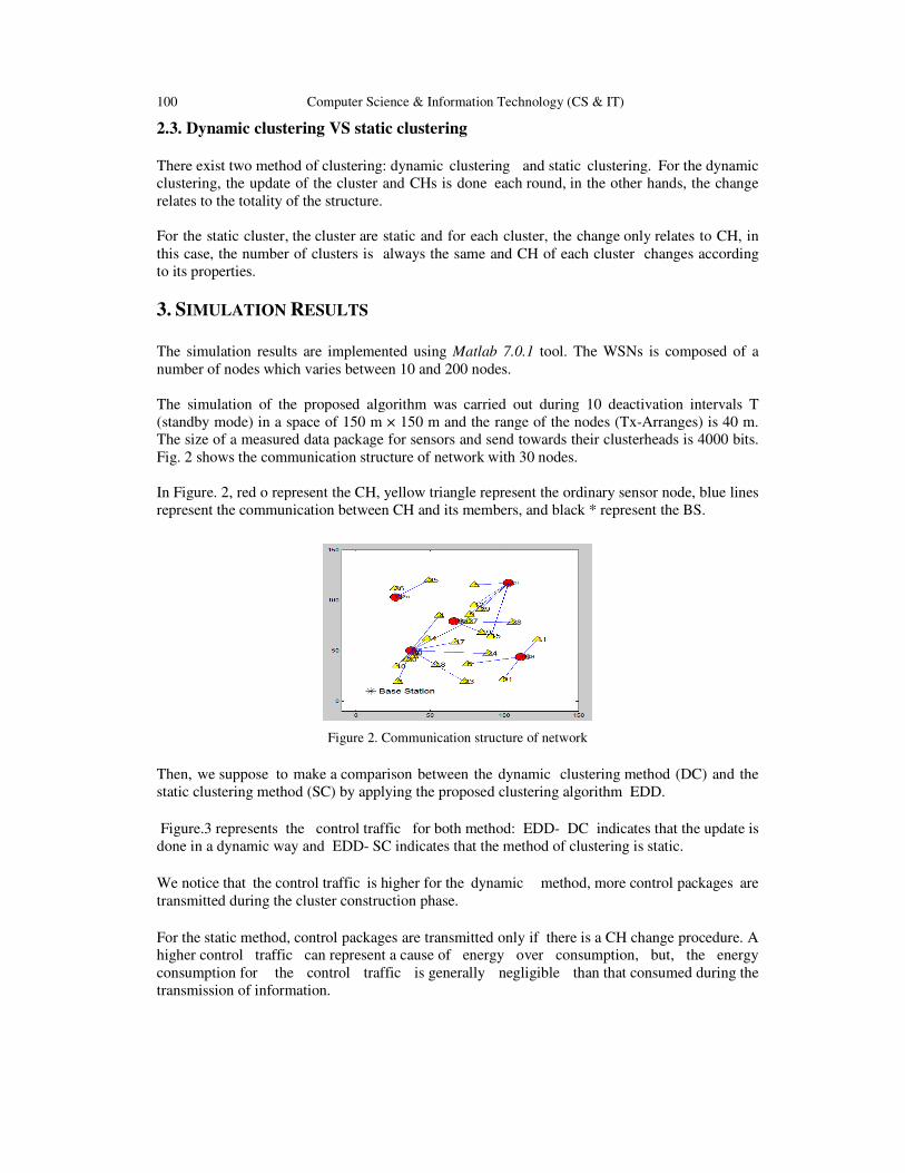
100 Computer Science & Information Technology (CS & IT)
2.3. Dynamic clustering VS static clustering
There exist two method of clustering: dynamic clustering and static clustering. For the dynamic
clustering, the update of the cluster and CHs is done each round, in the other hands, the change
relates to the totality of the structure.
For the static cluster, the cluster are static and for each cluster, the change only relates to CH, in
this case, the number of clusters is always the same and CH of each cluster changes according
to its properties.
3. SIMULATION RESULTS
The simulation results are implemented using Matlab 7.0.1 tool. The WSNs is composed of a
number of nodes which varies between 10 and 200 nodes.
The simulation of the proposed algorithm was carried out during 10 deactivation intervals T
(standby mode) in a space of 150 m × 150 m and the range of the nodes (Tx-Arranges) is 40 m.
The size of a measured data package for sensors and send towards their clusterheads is 4000 bits.
Fig. 2 shows the communication structure of network with 30 nodes.
In Figure. 2, red o represent the CH, yellow triangle represent the ordinary sensor node, blue lines
represent the communication between CH and its members, and black * represent the BS.
Figure 2. Communication structure of network
Then, we suppose to make a comparison between the dynamic clustering method (DC) and the
static clustering method (SC) by applying the proposed clustering algorithm EDD.
Figure.3 represents the control traffic for both method: EDD- DC indicates that the update is
done in a dynamic way and EDD- SC indicates that the method of clustering is static.
We notice that the control traffic is higher for the dynamic method, more control packages are
transmitted during the cluster construction phase.
For the static method, control packages are transmitted only if there is a CH change procedure. A
higher control traffic can represent a cause of energy over consumption, but, the energy
consumption for the control traffic is generally negligible than that consumed during the
transmission of information.

Computer Science & Information Technology (CS & IT) 101
Figure 3. Control traffic
Figure.4 represents the average energy consumption for both methods. We notice that the
average energy consumption of the dynamic method is higher, this method consumes more
energy during the cluster head election phase and the clusters update phase.
Figure 4. Energy consumption
Figure. 5 represents the first node die for two methods. The best results are given by EDD- DC,
this method tends to balance the load of energy consumption between nodes, in this case the
network lifetime increases. EDD- SC set up of the static clusters and the update concerne only
the CHs. This method can involves the choice of CHs having a weak energy reserve, which
results the crushing of its battery.

102 Computer Science & Information Technology (CS & IT)
Figure 5. First node die
Among the most known clustering algorithms in literature, we distinguish, LEACH algorithm [8].
LEACH is a famous algorithm which the goal is the minimization of the energy consumption in
the WSNs.
We wish in this part to compare our algorithm with the LEACH clustering algorithm. Figure. 6
represents the energy consumption VS the network size. We can note that the values obtained by
our algorithm are rather low compared to those obtained by LEACH. These results indicate that
our algorithm is more effective and can prolong the network lifetime and ensure its good
performance.
Figure 6. EDD-DC VS LEACH
3. CONCLUSIONS
We presented in this paper a new clustering algorithm for the WSNs called EDD. The principal
goal of our algorithm is the prolongation of the network life time, two parameters were taken into
account for the choice of CHs: the nodes energy consumption and their degree.
The simulation results show that our algorithm is more effective in energy and increase the
network lifetime.

Computer Science & Information Technology (CS & IT) 103
REFERENCES
[1] C. Tidjane Kone, (2011) ‘’Conception de l’architecture d’un réseau de capteurs sans fil de grande
dimension,’’PHD, University of Henri Poincaré Nancy I.
[2] G. Chalhoub, (2010) ‘’Les réseaux de capteurs sans fil’’, Ph.D, University of Clermont, Auvergne.
[3] L. Samper, (2008) ‘‘Modélisations et analyses de Réseaux de capteurs’’, PHD, VERIMAG laboratory.
[4] R. Kacimi, (2009)’’Techniques de conservation d’énergie pour les réseaux de capteurs sans fil,’’ PHD,
TOULOUSE UNIVERSITY.
[5] M. Khan & J. Misic. (2009) ‘’On the lifetime of wireless sensor networks,’’ ACM Transactions on
Sensor Networks (TOSN), Vol, 5, No. 5.
[6] R. Kuntz, (2010) ‘‘Medium access control facing the dynamics of wireless sensor networks, ‘‘PHD,
University of Strasbourg.
[7] D. Kumar, D. Trilok, C. Aseri & R. B. Patel, (2009) ‘’EEHC : energy efficient heterogeneous
clustered scheme for wireless sensor networks,’’ Computer Communication., Vol. 32, No. 4, pp 662–
667.
[8] W. B. Heinzelman, (2000) ‘’Application-specific protocol architectures for wireless networks,’’ PHD,
B.S.Cornell University.
[9] Y. Ossama & S. Fahmy, (2004) ‘’HEED : A hybrid energy-efficient distributed clustering
approach for ad hoc sensor networks,’’ IEEE Transactions on Mobile Computing, Vol. 3, No. 4,
pp 366 – 379.
[10] Duan, Changmin & Hong Fan, (2007) ‘' A distributed energy balance clustering protocol for
heterogeneous wireless sensor neworks''. In : Proc. Int. Conf. Wireless Communications, Networking
and Mobile Computing WiCom. pp. 2469–2473.
[11] V. Raghunathan, C. Schurgers, S. Park & M.B. Srivastava, (2002) ‘’Energy- aware wireless micro-
sensor networks,’’ IEEE Signal Processing Magazine, Vol. 19, No. 2, pp 40 –50.
[12] Mitton, Nathalie, Busson, Anthony & Fleury, Eric. (2004) ‘’Self-organization in large scale adhoc
networks‘’. In : Mediterranean ad hoc Networking Workshop (Med-Hoc-Net’04). Bodrum, Turquie.
[13] Wendi Rabiner Heinzelman, Anantha Chandrakasan, & Hari Balakrishnan, (2000) “Energy-efficient
communication protocol for wireless microsensor networks,” In : Proc IEEE 33rd Hawaii International
Conference on System Sciences.
[14] G. J. Pottie & W. J. Kaiser, (2000) ‘’Wireless integrated network sensors,’’ Commun. ACM, Vol. 43,
No. 5, pp. 51-58.
AUTHORS
Awatef BENFRADJ was born in Gabes, Tunisia in 1983. She received the engineering
degree in Telecommunications and Networks from the University of Gabes, in 2007. In
2009, she obtained the master degree in Networks from Higher School of Communication
of Tunisia. Since 2011, she has been a researcher within the laboratory of electronics and
information technology, Sfax University.
Salim El Khediri, a Ph.D student at the National School of Engineers of Sfax, Tunisia
(Laboratory of Electrical and Information Technology) and in partnership collaboration
education with CEDRIC laboratory of CNAM (National Conservatory of Arts and Crafts ,
Paris). Since 2009 working in the capacity of assistant teacher of computer sciences at the
Faculty of Sciences Gafsa – Tunisia.

104 Computer Science & Information Technology (CS & IT)
Nejah NASRI was born in Menzel Bouzaienne Village, in 1981. He received the B.S.
and M.S. degrees in electronic engineering from the University of Sfax, in 2006 and the
Ph.D. degree in electronic and telecommunication engineering from Toulouse University,
France, in 2010. From 2006 to 2009, he was a Research Assistant with Higher Institute of
Computer and Communication Techniques (ISITCom), Hammam Sousse, Tunisia. Since
2010, he has been an Assistant Professor with the Informatics Engineering Department,
Gafsa University. He is the author of more than 50 articles. His research interests include
engineering of wireless sensors networks and wireless underwater communication.
Abdennaceur KACHOURI was born in Sfax, Tunisia, in 1954. He received the
engineering diploma from National school of Engineering of Sfax in 1981, a Master
degree in Measurement and Instrumentation from National school of Bordeaux
(ENSERB) of France in 1981, a Doctorate in Measurement and Instrumentation from
ENSERB, in 1983. He “works” on several cooperation with communication research
groups in Tunisia and France. Currently, he is Permanent Professor at ENIS School of
Engineering and member in the “LETI” Laboratory ENIS Sfax

Natarajan Meghanathan et al. (Eds) : NeTCoM, CSIT, GRAPH-HOC, SPTM - 2014
pp. 105–117, 2014. © CS & IT-CSCP 2014 DOI : 10.5121/csit.2014.41309
VIDEOCONFERENCING WEB
APPLICATION FOR CARDIOLOGY DOMAIN USING FLEX/J2EE TECHNOLOGIES
Imen Debbabi and Ridha Bouallegue
Innov'COM Research laboratory, University of Carthage, Tunis, Tunisia.
[email protected] [email protected]
ABSTRACT The recent advances in computer technology and data networking have made videoconferencing
system a popular medium for users to interact with one another from remote locations. This
system offers communication between more than two users, who are able to interact through
their webcams, microphone and other components. The use of this system has been increased
recently due to many reasons, for one thing, progress in Internet access in different networks
like companies, universities and houses, with the increase of available bandwidth whereas the
decrease of delay in sending and receiving packets . On the other hand, the coming of Rich
Internet Applications (RIA) means that a large part of web application started to be
implemented on the web browsers. This paper discusses the conception of multiparty
videoconferencing systems using technologies of Web 2.0. For our conceptual
Videoconferencing Platform, we have developed many feature : live audio video, text
chat, video recording, user and room management and quality control. Videoconferencing
modules have been carried out using open source technologies Flex and J2EE.
KEYWORDS Videoconferencing System, RIA, web2.0, Flex, Red5, J2EE .
1. INTRODUCTION
Telemedicine is defined as the use of telecommunication and information technologies in order to
provide clinical health care at distance. It helps eliminate distance barriers and can improve
access to medical services that would often not be consistently available in distant rural
communities using two-way videos, emails, smart phones, wireless tools and other forms of
telecommunication technology [1].
It may be as simple as two health professionals discussing medical problems of a patient and
seeking advice from over a simple telephone to more complex transmission of electronic
medical records of clinical information, diagnostic tests such as E.C.G, radiological images etc .
and carrying out real time interactive medical video conference with the help of
Information Technologies.
This paper describes a videoconferencing system using open source technologies for a group of
cardiologists connected through internet. There may be a situation where a cardiologist in a
remote hospital may need to contact an expert to take his advice about a better treatment of a
patient. Videoconferencing enables a group of cardiologists to organize meetings, conferences,

106 Computer Science & Information Technology (CS & IT)
training or other distant meetings while giving the impression of being all present in the same
room.
In the recent years, the videoconferencing systems have become more complex due to increasing
demands of this type of systems in the internet and the heterogeneity of terminals, such as
laptops, mobile phones, tablets, etc with a variety of network access connections including
ADSL, cable Modem, Wi-Fi, UMTS, etc. On the other hand, the maturity of multimedia codecs,
formats and protocols has become a reality in the last decade. Therefore, a lot of
videoconferencing applications and solutions arise every year.
I.debbabi and al. [2] give a survey of the videoconferencing standards and videoconferencing
solutions and compare them. These systems are provided in two different ways. The first type is
the centralized system. Generally, drawbacks of the centralized system are not scalable and the
operations of the MCUs (Multipoint Conference Unit) are very complex and expensive. The
outgoing bandwidth of the server is shared by all the concurrent participants. Specifically, the
more clients there are, the lesser the bandwidth each participant can have. The more
expensive multipoint control units are capable of handling more connections, the faster data
transfer rate is and the more participants can be displayed on the video screen at one time. In
addition, MCU requires a higher bandwidth to disseminate a single video signal among
participants. The second kind of videoconferencing system is the multicast videoconferencing
system. It is often free of charge and easy to install and use, although quality cannot be
guaranteed.
In the traditional systems, videos, audios and document information encoding, decoding and
transfer are implemented by the developers, which makes the systems more difficult to be
developed, and the deployment and maintenance more expensive. These Desktop applications
have a difficult installation, maintenance and access flexibility for many reasons like the
increasing number of clients with different hardware and operating systems. Web developers
have always tried to build one type of client which is richer, more powerful and sensitive and
have more interesting visual characteristics than the traditional HTML. The appearance of RIA
technology makes it possible to deploy rich client program as easily as to use the web on the
Internet.
In this paper, we present a technical overview of technologies for Rich Internet applications,
Red5 Media Server, J2EE framework and Flex technologies .We also present architecture of
videoconferencing system using these technologies. The remainder of this paper is organized as
follows: Section 2 presents some technologies of RIA .Section 3 presents the design of our
system. In Section 4, we present the realization of the system. Section 5 describes the conclusion
and future work.
2. TECHNICAL OVERVIEW
2.1 Technologies for Rich Internet application
The term ”Rich Internet Applications” was introduced in a Macromedia whitepaper [3] to
designate a unification of desktop and traditional Web applications whose goal is to take the
advantages of both architectures and overcome their disadvantages. “Macromedia “define RIAs
as combining the best user interface functionality of desktop software applications with the broad
reach and low-cost deployment of the web applications and the best of interactive multimedia
communication.
Typically, a RIA is a web application running in a web browser as part of a web site and is loaded
by the client along with some initial data, then it manages the data rendering and event

Computer Science & Information Technology (CS & IT) 107
processing, communicating with the server only when the user requires further information or
must submit the data. However, this type of application shares several characteristics like a rich
user experience and complex user interfaces with traditional desktop applications, and can be
accessed using only the web browser with the use of JavaScript; via a browser plug-ings or
sandboxes. It forces the users to install a plug-in before launching the application. Once installed,
the application runs inside a sandbox delivered within the plug-in.
Before viewing a list of Rich Internet Application frameworks, we should know that a framework
is a collection of software libraries providing an application programming interface (API), which
provides generic functionality that separates them from other normal libraries.
In the case of RIAs, there is an extensive list of software frameworks that can be useful in
different contexts, with different programming languages and operating systems. The vast
majority of frameworks are intended to run over almost all the operating systems.
These Frameworks are Adobe Flash, Microsoft Silverlight, Oracle Java FX, AJAX or HTML5.
They have to be installed on clients that are going to run these applications.
Many studies regarding the installation made depict the market penetration and global usage
comparing different technologies. They show that Adobe Flash, Microsoft Silverlight and Java
are installed in more than 60% of machines.
2.1.1 Adobe Flash Player
Adobe Flash (formerly Macromedia Flash) is a multimedia platform used to add animation,
videos, and interactivity to web pages. Flash is frequently used for advertisements and games.
More recently; it has been positioned as a tool for the Rich Internet Application .It is mainly
based on an object-oriented language named ActionScript.
In order to run the Flash content, the users need to install the Flash Player plug-in previously.
Nowadays, Flash content may be displayed on various computer systems and devices using
Adobe Flash Player, which is free for common web browsers, some mobile phones and a few
other electronic devices (using Flash Lite).When Flash Player starts running the application, it
manipulates vector graphics to provide animation to various components, like text, drawings,
images, and UI objects. It also provides advanced APIs, such as the possibility of manipulating
images directly, audios and videos. It supports multimedia streaming applications, such as videos
and audios streaming as well as bidirectional multimedia communication and can capture the
user’s input via a mouse, a keyboard, a microphone, and a camera.
2.1.2 Real Time Messaging Protocol (RTMP)
The protocol called Real Time Messaging Protocol (RTMP) was initially implemented by
Macromedia in 2002 and now it is owned by Adobe. It was first used to stream the content across
the internet from the servers to the clients which were applications running in a web browser
plug-in (Macromedia Flash Player). It was then used to implement web conferences, by accessing
the user’s camera and microphone through the same clients, and then sending them using RTMP
to send and receive media flows. In 2009, having acquired Macromedia, Adobe decided to
publish an open specification of this protocol in [4].
According to those specifications, the RTMP protocol has multiple variations, i.e. the “plain”
RTMP protocol; RTMPS which is RTMP over a TLS/SSL connection, RTMPE which is RTMP

108 Computer Science & Information Technology (CS & IT)
encrypted using Adobe’s own security mechanism, and RTMPT which is encapsulated within
HTTP requests to go through firewalls [4].
RTMP works on top of TCP which maintains persistent connections and allows low-latency
communication. It originally follows client-server architecture by defining requests and
responses. This protocol splits media streams into fragments and their size is negotiated
dynamically between the client and the server. Thus, it transmits as much information as possible
with a little overhead.
RTMP defines several virtual channels to provide multiplexing of audios, videos and data sent in
the same TCP connection. It defines headers like a timestamp, size of packet, id of the channel, as
shown in Fig 1.
AT higher level, RTMP encapsulates MP3, AAC and Speex audio, FLVI and H.264 video, and
can make remote procedure calls (RPCS) using a specific format for the representation of the
data, named Action Message Format (AMF)[4].
Figure 1 : RTMP packet structure
2.2 Red5 Media Server
The development of Flash-based applications requires the implementation of a centralized Server
architecture based on a multimedia server, which redirects all the traffic sent between clients, for
example Adobe Flash Media Server. This server is a new platform used for communication
between users. It integrates Flash multimedia interactive features, and adds real-time audio,
real-time video and real-time data streams and other new features like broadcasting. This
server is proprietary media server from Adobe Systems but not free. In this work, we need an
open system server. There is an open source technology, called Red5 Media Server, which
delivers a powerful video streaming and multi-user solution to the Adobe Flash Player and other
exciting client technologies [4].
Red5 is an open source software package written in the Java language. Its purpose is to
consolidate communication between Adobe flash applications. It offers the same functionality as
Adobe Flash Server. It supports live stream publishing, audios and videos streaming, object
sharing as well as the recording of streams [6, 7].
By using this platform, you can save recorded audios, videos from a network, share data objects,
and transfer the audios, videos and shared data objects with multiple clients. Therefore, it stands
as a solid solution for businesses of all sizes, such as enterprises and it is widely used for
developing videoconferencing systems, multi-user gaming and enterprise application software.
Red5 includes a support for the latest multi-user APIs such as NetConnection, NetStream and
SharedObject while providing a powerful RTMP / Servlet implementation. In addition to

Computer Science & Information Technology (CS & IT) 109
supporting the RTMP protocol, the application server has an embedded Tomcat Servlet container
for JEE Web Applications.
In Red5, we developed a browser based videoconferencing application. Here, the client uses
Adobe Flash Player to capture videos and audios from players continuous media clips from a web
server. This platform integrates communication and application functions, via a flash player on
the client, captures and shares audios, videos and data streams. By using Red5 and Flex, we can
easily create a real-time communication system, which allows two or more end-users to
communicate instantly. For example, we can use the Red5 to easily create video conferencing
systems, video telephone system and video chatting systems [6, 7].The system presented here is
designed based on Flex. It uses extended UI component library and defines rich user interface on
MXML.
Macromedia Flex is a representing server and application program framework, which meets the
needs of enterprise-class programmers who hope to develop RIA and run on J2EE. It can run in
the application server and provide standard-based, declarative programming methods and
processes, run-time services, application integration and management capabilities.
Flex can integrate Java object access or xml using the existing code and information.
Furthermore, Flex can also be integrated with some of the existing presentational technology and
framework, such as JSP, Struts, etc [8].
In addition, it deals with procedure logic by using script towards objects, and runs swf client
program translated by Flex server into Flash Player. Combining with audio, video and some
real-time communication technologies, the RIA has highly interactive user experience.
2.3 J2EE Framework
J2EE is a set of specifications, which define the standard for developing multi-tier enterprise
applications with Java. This platform provides a complete framework for design, development,
assembly, and deployment of Java applications built on multi-tiered distributed application
model. This specification defines numerous API services and multiple application programming
models for developing applications and integrating them with the enterprise systems as shown in
Figure 2.

110 Computer Science & Information Technology (CS & IT)
Figure 2: Architecture of J2EE framework
A J2EE application is divided into multiple layers, as seen in Figure 2. Applications can have
three or four layers, although most of them only have three [8, 9].
The top layer exists on the client’s machine called The Presentation Layer. It consists mainly of
interactive webpage interfaces, but occasionally contains some functionality. This layer is
responsible for the management of the user's request and for making the corresponding
response. Example of the frameworks is Struts [9].
The next level is the Web tier. This level may contain Java Server Pages (JSPs) and servlets,
which dynamically handle requests to the server. The Web tier is usually excluded, in which case
the Client tier interacts directly with the Business layer. This latter layer holds the enterprise
beans, which retrieve and process the data from the database.
This layer is responsible for dealing with application procedure business logic and business
checking, and responsible for the management services .An example of this framework is
Spring[9].
Finally, the Enterprise Information System (EIS) layer is the database in which the information is
stored. This layer is responsible for building a relationship between the java domain objects
and the database tables. An example of this framework is Hibernate [9].
The Business layer is responsible for dealing with application procedure’s business logic and
business checking, and responsible for the management services. An example of this framework
is Spring.

Computer Science & Information Technology (CS & IT) 111
2.4 Integration of Flex and J2EE
Prior to the release of Flex, J2EE developers could tightly integrate their middleware with a
Flash-based client by using the Flash Remoting technology. This was introduced by one of the
authors in the Macromedia Press title Reality J2EE—Architecting for Flash MX.
As shown in Fig.3, Flex is integrated in the Presentation Layer. Flex communicates with the
Business Layer through the AMF gateway. The advantage of this model is that it can
quickly and conveniently integrate the Flex into the existing J2EE framework without
affecting the original structure [8].
Introducing Flex into data services will affect the performance of Flex. Flex offers several ways
to send data: calling the Java classes loaded in Flex classpath; sending a request to the web
proxies service or HTTP server [8]. Flex data services can be divided into Web Service
Agent, remote object proxy and HTTP services, etc. Two better choices are the XML of HTTP
Service and AMF's Remote Object [8].
In this framework, a statement which appeared in the Flex page announces that a Remote object
(FlexFacade type) run on the server-side. Flex is responsible for the data transfer between Flex
pages and Java objects. We need to define a corresponding method in an object when the Java
method is necessary in all the Flex pages which will call the corresponding method in Flex
Facade object, and then the method will call the Java method which realizes the business logic
in the background [8].
Figure 3: Integrable framework of Flex/Struts
3. SYSTEM DESIGN
3.1 Design of Videoconferencing system
In recent years, more and more multimedia conference systems have been deployed on the
Internet. A typical Videoconferencing System has the following functionalities : Live Audio /
Video, Text Chat and Video Recording .Firstly, the live audio / video tool supports multiple
video displays, showing the video streams from the cameras focusing on the different remote
cardiologists. Next, the Text Chat facilitates chatting amongst cardiologists sitting in remote
place. Finally, the video Recording helps automatically record and save all the videos in a central
archive, where cardiologists can access them conveniently when they need to review them.
Our videoconferencing prototype has four main modules as demonstrated in Fig. 4.

112 Computer Science & Information Technology (CS & IT)
Figure 4: Prototype Videoconferencing System
� Audio/Video and Text Tchat Module: This module captures the videos, relays it to the
receiver’s end to enable cardiologist sitting in remote place chat with one another.
� File Sharing and Recording Module: This module helps the users share files and record
their video/audio conferencing and text chatting through the internet.
� User and Room Management Module: The purpose of this module is the authentication
and identification of the registered users. It also facilitates the connection between the
user groups for audio/video conferencing.
� Quality Control Module: The role of this module is to control the quality of images and
audios and capture the videos and relays them to the receiver's end with a desired quality
of service.
3.2 Implementation of Videoconferencing system
The architecture of our application is client-server, where a computer interacts with others on the
Internet.
As we mentioned earlier, our application consists of three parts: User and Room management
developed in Jsp / Servlet / JavaBeans, some for streaming videos developed in Flex (MXML,
Action Script) and a portion for controlling a PC remotely with suitable tools like VNC viewer
open sources and VNC server.
To do so, we need:
� On the application server: Apache Tomcat is used as an application server for the
management of the rooms and users.
� On the streaming server (Red5): It is responsible for disseminating all the information
Multimedia (video, micro, slides) to all the participants.
� On the MySQL database server: handles the data storage.
� A thin client: a web browser (Google Chrome, Firefox ...)

Computer Science & Information Technology (CS & IT) 113
Figure 5: Architecture of application
In the realization of our project, we opted for MVC architecture to provide insurance
maintainability, scalability of the application and the speed of development. The Figure 5 shows
the architecture of our application.
4. REALIZATION
The implementation of the proposed architecture in this paper has resulted in the provision of a
system that consists of a set of classes and methods that we will detail in this section.
4.1 Several important classes and methods
4.1.1 Class Application
Application class contains information about a Red5 Server application. It maintains this
information until the application program is unloaded.
There are several important events in the application class:
� AppStart: it is called when the applications are loaded.
� AppStop: it is called when the applications are uninstalled.
� Connect: it is called when a client connects with the application.
� Disconnect: it is called when a client disconnects with the application.
There are several important methods in the class Application:
� acceptConnection: it accepts the connection from a client to an application procedure.
� broadcastMsg: it announces the news to all the connected clients.
� disconnect: it disconnects the connection between the server and the clients.
� rejectConnection: it refuses an application to another.

114 Computer Science & Information Technology (CS & IT)
4.1.2 Class NetConnection
NetConnection is used for the management of a two-way connection between Flash Player and
red5 Server. It can let you connect to the remote Flash object and red5 Server, while red5
Server allows you to use macromedia Real-Time Messaging Protocol to share audio, video
and data information.
4.1.3 Class NetStream
NetStream realizes a data stream connection between Flash Player and Red5 Server. A
NetStream object is just like a channel of a NetConnection objects. This channel can, by using
the publication method of NetStream object, publish audio and video data, or by using Play()
method of NetStream objects, subscribe a pubished flow or data. When necessary, we can
also, using NetStream object, publish or broadcast live video and audio information, or play
previously recorded video and audio information. There are two important methods in
NetStream object: NetStream.attachAudio() and NetStreamattachVideo(). These two methods
are essential for the network video call. We can make use of these two methods to bind
the audio from the microphone, and the video from the camera with a network stream.
4.1.4 Server-side programming
Service-side scripting can be used to control log-in processes, and control the events in
connection Micromedia Flash program which determine the data that the users get from
the Flash program. Server-side script file is generally main.asc. When the system is running,
the file is placed in the Applications directory of the Flash Media Server. Service-side
scripting main code is as following:
userList=[];
application.onConnect = function(currentClient)
{
application.acceptConnection(currentClient);
currentClient.communicateServer= function(value)
{
currentClient.username=value;
userList.push(value);
trace("The current user list"+userList);
application.broadcastMsg("playOtherVideo",userList);
}
}
4.1.5 Client Programming
The release and acceptance of video and audio signals is realized by NetStream object of red5
Server. It mainly constructs a TCP-based connection by using the RTMP agreement, between the
client and FMS. A connection can contain several RTMP data circulation channels. When the
clients log in video conferencing systems successfully, FMS uses a data flow channel to publish
the user's video and audio streams. At the same time, FMS, by using several data flow
channels, receives other client user's video and audio stream.
The following is the registered user’ video, audio stream core code, published by FMS.
First of all, the client to establish connection:

Computer Science & Information Technology (CS & IT) 115
var RTMP = " rtmp ://localhost:5080/Videoconference" ;
_global.out_nc = new NetConnection () ;
out_nc. connect (RTMP ,PhoneID) ;
var mic = Microphone.get() ;
mic.setRate (11) ;
mic.setUseEchoSuppression (t rue) ;
mic.setSilenceLevel (0 , 0) ;
Publish the audio stream of our side to the user:
outAudio_ns = new NetStream(out_nc) ;
outAudio_ns.attachAudio(mic) ;
outAudio_ns.publish("Audio" + PhoneID) ;
Publish the video stream of our side to the user:
outVideo_ns =new NetStream(out_nc) ;// New data streams
outVideo_ns.attachVideo (Camera.get()) ;
outVideo_ns.publish("Video" + OutID) ;
Accepting the video stream of other side:
inVideo_ns = new NetStream(out_ nc); // new data streams.
Video_AV.attachVideo(inVideo_ns);//
inVideo_ns.play("Video " + PhotoNum_ mc.CallOutNum) ;
4.2 Comparative study and discussions
Traditional video conference systems have problems of development, expensive deployment and
maintenance. Flex and Red5 Server provide a new and better solution to develop videos, webcast,
MP3 streaming audios, videos conferencing and audio and video chat. This application combines
the best user ‘s interface functionality of desktop software applications with the broad reach and
low-cost deployment of Web applications and the best of interactive, multimedia communication.
Among the different applications of videoconferencing proposed in literature we have described
only a few examples in this section.
Ponec et al. [11] considered P2P multi-rate multi-party conferencing systems. In a multi-rate
setting, different receivers in the same group can receive video at different rates using layered
videos. In particular, their study focuses on issues related to multi-rate setting in comparison to
the case of single rate videos. It studies the optimal usage of peer uplink capacities of P2P utility
maximization in a multi-rate multicast which provides a novel multi-tree formulation.
Nefsis [10] provides dedicated cloud computing resources for video conferencing. The users
automatically connect to geographically close servers distributed on the Internet to have a low-
latency experience.
We now consider well known, free or commercial conferencing systems such as Skype, Gmail
chat and Apple’s iChat, and discuss how they address the challenge of Multipoint conferencing.
Skype provides multipoint audio conferencing, but video conferencing in Skype is only point-to-
point. Recently, the developers have added a group feature which is limited to 5 persons;
however, it is not known what the bandwidth requirements are.
GMail chat has a video conferencing module (Google gmail chat), but it works only for two
persons. Moreover, it uses a special hardware provided by Vidyo.

116 Computer Science & Information Technology (CS & IT)
Apple’s iChat provides multipoint video conferencing; however, one of the peers has to have
enough download and upload bandwidth to initiate the conference where it presumably acts as a
software MCU (Multipoint Multipoint Control Unit : Apple iChat).
Many other popular online chatting applications (like Skype, Msn, Yahoo, messenger, Google
talk, etc.) support multi-party videoconference but they have not a good quality of service
therefore, they are not utilizable for professional use like in telemedicine and therefore not
considered here.
We have considered Tree applications, of which we list the maximum bandwidth, the delay, the
technique of video coding, the maximum number of simultaneous conference participants, and
the architecture (S/C or P2P) they belong to Table 1.
From Table 1, we observe that all the applications support only a very limited number of
participants and the applications that support more than 10 simultaneous participants,who all use
a centralized or P2P network structure.
Table 1 : A comparison of videoconferencing solutions
Delay in
ms
Bandwidth
kbps
Number of
Video
participants
Video coding Architecture
Ponec and
al.,[11]
<100 2000 15 H.264/AVC
Distributed P2P
Nefsis
[10]
20 14Mbps 8 - centralized
Our
application
<100 2500 8 - centralized
We observe that the maximum bandwidth is 14 Mbps which corresponds to cloud computing
solutions whereas the second bandwidth is 2.5 Mbps which corresponds to our web application.
The solutions based on P2P architecture features of the best bandwidth and the best delay is
inferior to 100 ms.
3. CONCLUSIONS
Videoconferencing systems have problems of development and expensive deployment. In this
paper, we provide a new method using open source technologies based on the Flex and J2EE
video conferencing network system to develop a low cost one. It is intended to support
consultations for a group of cardiologists connected through the internet.
For future work, Videoconferencing System with 3G and 4G mobile telephony and virtual
reality technologies can be developed.
REFERENCES
[1] http://www.americantelemed.org/about-telemedicine/what-is-telemedicine.
[2] I.Debbabi,”A Survey of multimedia videoconferencing system and a proposal for a novel hybrid
cloud and P2P architecture”. ISSN 22773061. 1641 | Page. Aug 20, 2013.
[3] J. Duhl. White paper: Rich Internet Applications.Technical report, IDC, November 2003.
[4] Adobe Systems Incorporated, Adobe’s Real Time Messaging Protocol specification , 21 December,
2012.
[5] http://www.red5.org/

Computer Science & Information Technology (CS & IT) 117
[6] Liu Lu and Dong XiaoGuo, 2010. Red5 flash server analysis and video call service implement-
tation. In Proceedings of IEEE symposium on web society, pages 397-400.
[7] X. C. Peng, “The Integration of Flex RIA with J2EE Application,” Application Technology and
Research, June, 2008, pp. 37-39 (in Chinese).
[9] http:/java.sun.com/j2ee.
[10] http://www.nefsis.co Nefsis. Online: http://www.nefsis.com/How-Multipoint-Conferencing-
Works/index-multipoint-video-conferencing.htmlS.
[11] Ponec, M., S. Sengupta, M. Chen, L. Jin and P.A. Chou, 2009. “Multi-rate peer-to-peer video
conferencing: A distributed approach using scalable coding. Proceedings of the IEEE International
Conference on Multimedia and Expo, Ju. 28-Jul. 3, IEEE Xplore Press, New York, pp: 1406-1413.
DOI: 10.1109/ICME.2009.5202767
AUTHORS
Imen debbabi was born in Monastir ,Tunisia, in 1984. She received the B.S. degree in
Computer engineering from National Engineering School of Sousse, Tunisia, in 2008,
and a master degree of “Intelligent and Communicating Systems “from National
Engineering School of Sousse, Tunisisa, in 2010. She is currently pursuing Ph.D
degree in Higher School of communication, Tunis, Tunisia. Her research interests
include, Multiparty Video Conference and multimedia System .

118 Computer Science & Information Technology (CS & IT)
INTENTIONAL BLANK

Natarajan Meghanathan et al. (Eds) : NeTCoM, CSIT, GRAPH-HOC, SPTM - 2014
pp. 119–130, 2014. © CS & IT-CSCP 2014 DOI : 10.5121/csit.2014.41310
ALAMOUTI OFDM/OQAM SYSTEMS WITH
TIME REVERSAL TECHNIQUE
Ilhem Blel and Ridha Bouallegue
Innov’Com Laboratory Higher School of Communications,
University of Carthage, Tunis, Tunisia [email protected]
ABSTRACT
Orthogonal Frequency Division Multiplexing with Offset Quadrature Amplitude Modulation
(OFDM / OQAM) is a multicarrier modulation scheme that can be considered as an alternative
to the conventional Orthogonal Frequency Division Multiplexing (OFDM) with Cyclic Prefix
(CP) for transmission over multipath fading channels. In this paper, we investigate the
combination of the OFDM/OQAM with Alamouti system with Time Reversal (TR) technique.
TR can be viewed as a precoding scheme which can be combined with OFDM/OQAM and
easily carried out in a Multiple Input Single Output (MISO) context such as Alamouti system.
We present the simulation results of the performance of OFDM/OQAM system in SISO case
compared with the conventional CP-OFDM system and the performance of the combination
Alamouti OFDM / OQAM with TR compared to Alamouti CP-OFDM. The performance is
derived by computing the Bit Error Rate (BER) as a function of the transmit signal-to-noise
ratio (SNR).
KEYWORDS
OFDM/OQAM, Alamouti, OSTBC, Time Reversal
1. INTRODUCTION
The use of radio communication systems with multiple transmit and receive antennas also
referred to as MIMO system can be used to increase capacity. Because of the time-dispersion that
occurs in radio mobile communications, the MIMO channel is frequency selective.
OFDM presents the property to convert such a frequency selective MIMO channel into a set of
parallel frequency flat MIMO channels. This makes CP-OFDM a suitable scheme to be
associated with MIMO.
Standards such as IEEE802.11a have already implemented the CP-OFDM. Other standards like
IEEE802.11n combine CP-OFDM and MIMO in order to increase the bit rate and to provide a
better use of the channel spatial diversity.

120 Computer Science & Information Technology (CS & IT)
Nevertheless, CP-OFDM technique causes a loss of spectral efficiency due to the CP as it
contains redundant information. Moreover, the rectangular prototype filter used in CP-OFDM has
poor frequency localization which makes it difficult for CP-OFDM systems to respect stringent
specifications of spectrum masks.
To overcome these drawbacks, OFDM/OQAM was proposed as an alternative approach to
CPOFDM. Indeed, OFDM/OQAM does not need any CP, and it furthermore offers the
possibility to use different time-frequency well localized prototype filters such as Isotropic
Orthogonal Transform Algorithm (IOTA). One of the characteristics of OFDM/OQAM is that the
demodulated transmitted symbols are accompanied by interference terms caused by the
neighboring transmitted data in time-frequency domain. The presence of this interference is an
issue for some MIMO schemes and until today their combination with OFDM/OQAM remains an
open problem.
Some interesting researches [1] [2] [3] propose a modification in the conventional
OFDM/OQAM modulation by transmitting complex QAM symbols instead of OQAM ones. This
proposal allows to reduce considerably the inherent interference but at the expense of the
orthogonality condition. Indeed, the data symbol and the inherent interference term are both
complex.
Regarding Alamouti coding, some works have been carried out such as [4] where the authors
showed that Alamouti coding can be performed when it is combined with code division multiple
access (CDMA). A pseudo-Alamouti scheme was introduced in [5] but at the expense of the
spectral efficiency since it requires the appending of a CP to the OFDM/OQAM signal. Another
solution was proposed in [6] where the Alamouti coding is performed in a block-wise manner
inserting gaps (zero-symbols and pilots) in order to isolate the blocks. The main objective of this
paper is to analyze and study the combination of OFDM/OQAM technique with Alamouti system
using Time Reversal approach.
Firstly experimented in acoustics and ultrasound domains [7] [8] [9], Time Reversal (TR) has
also received attention recently for wireless communications [10] [11] [12]. Owing to its inherent
time and spatial focusing properties, TR is now studied as a solution for future green wireless
communications [12]. Its time focusing property allows having low intersymbol interferences
(ISI) at the receiver side.
In fact, TR was highlighted to be suitable for MISO systems as it is simple prefiltering techniques
for any number of transmit antennas and leads to low complexity receivers [13]. Moreover, it
reduces the delay spread of the channel [14]. However, to achieve good performance in terms of
delay spread reduction and spatial focusing TR must be realized either over a large frequency
bandwidth or with multiple antennas [15].
Multicarrier systems such as OFDM are commonly used to deal with time-dispersive channels
and can be combined with TR to accommodate any residual intersymbol interference.
The combination of TR and OFDM has recently been studied in [11] [12] and has been proven to
allow designing of simple and efficient MISO-OFDM systems [16] [17]. In this paper we
investigate the combination of Alamouti OFDM/OQAM with TR.

Computer Science & Information Technology (CS & IT) 121
The remaining of this paper is organized as follow: In section II we describe the OFDM/OQAM
modulation in SISO case, and we show that the introduction of appropriate pulse shaping can
efficiently combat time and frequency distortions caused by the channel. In section III we present
the combination of OFDM/OQAM with multiple transmit antennas and especially with classical
Alamouti scheme using TR technique. In section IV we provide simulation results, and finally we
give the general conclusions in section V.
2. SINGLE-INPUT SINGLE-OUTPUT OFDM-OQAM
The OFDM/OQAM signal in baseband and discrete time for M subcarriers can be expressed, at
time kTe, as follows:
(1)
Where Te denotes the sampling period, am,n are the real coefficients, f[] is a prototype filter of
length LF and denotes a phase term selected for example equal to . Thus, the
OFDM/OQAM modulation overcomes the presence of a guard interval or cyclic prefix thanks to
a judicious choice of the prototype filter modulating each subcarrier signal which enables well
localization in time and frequency, and which verifies the constraint of real orthogonality
between subcarriers resulting in:
The prototype filter has to satisfy the orthogonality conditions or at least must be nearly
orthogonal. It can be derived directly in continuous-time, as it is the case for instance in [18] with
the IOTA filter.
Naturally, the resulting prototype filter has to be truncated and discretized to be implemented.
The IOTA prototype filter used in this paper is of length L = 4M and it is denoted by IOTA4.
Prototype filters can also be directly derived in discrete time with a fixed length [19]. This is the
case of the time frequency localization (TFL) [19] prototype filter. In this paper, it is taken of
length L = M and denoted by TFL1.
The block diagram in Figure 1 illustrates our OFDM/OQAM transmission scheme in SISO case.
The pre-modulation steps corresponds to a single multiplication by an exponential which
argument depends on the phase term Φm,n and on the prototype length. The polyphase block
contains the coefficients of the prototype filter. At the receiver side the dual operation are carried
out that, at the end taking the real part of the post-demodulator output, allows us to exactly
recover the transmitted symbols in the case of a distortion-free channel.

122 Computer Science & Information Technology (CS & IT)

Computer Science & Information Technology (CS & IT) 123
Figure 1. OFDM/OQAM transmission scheme in SISO case
3. ALAMOUTI-OFDM/OQAM WITH TIME REVERSAL
Some works [1][2][3] show that when combining OFDM/OQAM with MIMO techniques such as
STBC, the presence of the interference term causes problems and makes the detection process
very hard if not impossible.
In this section, we shall propose a new Alamouti-OFDM/OQAM scheme in order to get rid of the
inherent interference term. Indeed, we will apply the time reversal technique on the outside of the
OFDM/OQAM modulator on each transmission antenna.
TR principles are presented in detail for acoustic and electromagnetic waves in [12] and [13]
respectively. Applied to wireless communications, TR consists in prefiltering the signal with the
time reversed and conjugated version of the channel impulse response (CIR) between transmit
and receive antennas. Without loss of generality, such an operation can be represented in discrete
time domain as depicted in Figure 2. In this figure, c[l] is the transmit shape filter, h[l] the
discrete complex-baseband CIR, h*[−l] the time reversal filter, and c[l] the so-called equivalent
channel obtained by convolving h[l] and h*[−l].
Consequently, in the time domain, c[l] is made of a central peak of high amplitude and some side
lobes. For rich propagation environments, a time focusing effect is obtained as the channel
autocorrelation peak is getting sharper and narrower and as side lobes are reduced. In other
words, TR leads to time dispersion compression, here by reducing the ISI occurring between
symbols [14].
Figure 2. Transmission with Time Reversal technique

124 Computer Science & Information Technology (CS & IT)
If time focusing is sufficiently strong for a given symbol duration, the receiver could merely be
reduced to a threshold detector. Nevertheless, for systems exploiting a restricted bandwidth or a
limited number of transmit antennas, residual ISI can be efficiently treated through multicarrier
approach. The TR and multicarrier approaches can be viewed as complementary and compatible
processes applied on the signal before transmission, the former trying to compress the channel
time dispersions and the latter accommodating with the residual ISI.
In some preliminary work [16] [17], it has been demonstrated that TR can be applied in an
OFDM system either in the time or in the frequency domain. For both implementations, the
achieved performance is equivalent.
On that basis, applying TR to an OFDM/OQAM signal amounts to precoding the symbols on
each subcarrier by the conjugated channel coefficients. These channel coefficients are obtained
from the frequency version of the CIR through a Fourier transform.
More precisely, we proposes to transmit OFDM/OQAM symbols associated with a transmit
antenna on an equivalent channel resulting from the convolution of the TR prefilter and the CIR.
Let us suppose that the transmission channel is a frequency selective channel consisting of L
paths. We denote h = (h0,h1,….,hL-1) the vector of the complex channel coefficients. In the
following description, are used indifferently channel coefficients, the temporal impulse response
or its transformation in Z to describe and qualify the transmission channel. These various
representations are equivalent. It will be the same for the TR prefilter.
These coefficients are distributed according to a centered Gaussian distribution. The transform in
Z of the impulse response h(t) of the transmission channel is H(z).
The time reversed from the transmission channel has as a transform and its impulse
response is h *(-t)
The equivalent channel seen by OFDM/OQAM modulation in frequency domain is thus:
(7)
The equivalent channel is thus a symmetric conjugate channel which central path c0 is a real
coefficient. It also appears, in light of the above equations, that because of the symmetry of the
coefficients of the equivalent channel, its transform C(z) is a real function. It will be noted that
this reasoning is valid for a discrete or continuous representation of the considered channel. This
means that the constraint of real orthogonality between the subcarriers verified by the prototype
filter is advantageously verified after passing through this equivalent channel since its equivalent
frequency response filter is real, even if the transmission channel associated with each antenna is
complex. This avoids the generation of an intrinsic interference term purely imaginary difficult to
remove such as that generated for a modulation OFDM/OQAM state of the art.
The diagram in Figure 3 illustrates the principal steps of an OSTBC-MISO-OFDM/OQAM
transmission scheme with TR technique. In this paper, we consider the Alamouti system with two
transmit antennas and one receiver antenna.

Computer Science & Information Technology (CS & IT) 125
Indeed a sequence of bits is transformed into a sequence of real symbols of QAM constellation.
Real symbols are then distributed over M subcarriers and two antennas in a step of serial-parallel
conversion, so as to form OFDM/OQAM symbols in the frequency domain for each transmit
antenna. There is a real symbol anm associated with the subcarrier m at time n. The real symbols
anm are then coded at OSTBC coding step according its spatial and temporal dimension to
generate two sequences of coded symbols for two transmit antennas. Such codes are described in
particular in [20] and in [21] for any number of transmit antennas. In this paper, we consider a
space-time coding of real symbols amn distributed over M subcarriers, defined by the following
real orthogonal coding matrix GR2:
Thus, during the OSTBC coding step, the matrix GR2 is applied to each subcarrier m. Thus
obtaining two sequences of coded symbols which are then respectively modulated for the two
transmit antennas in accordance with the OFDM/OQAM modulation scheme, and then converted
according to an operation of parallel-serial conversion carried out independently for each
antenna.
Then, for each Txj antenna, j=1,2, the OFDM/OQAM symbols forming coded OFDM/OQAM
multicarrier signal S(j) are filtered by a TRj prefilter defined from an estimate transmission
channel.
(8)
Multicarrier filtered signals x(j) are then transmitted over the propagation channel via their
respective transmit antennas.
Figure 4 illustrates the principal steps of an OSTBC-Alamouti-OFDM/OQAM reception scheme
where the received signal equal to the sum of the received signals from each transmit antenna is:
(9)
Where denotes an additive white Gaussian noise.

126 Computer Science & Information Technology (CS & IT)
Figure 3. OSTBC-MISO-OFDM/OQAM transmission
The multicarrier signal y', as depicted in Figure 4, are distributed in a serial-parallel conversion of
M subcarriers, and then an FFT operation is applied to demodulate OFDM/OQAM symbols.
Figure 4. OSTBC-Alamouti-OFDM/OQAM reception scheme
We note HR the equivalent channel obtained by convolution of hTR
and h.
With space-time coding GR2 matrix considered previously, the symbols obtained after FFT
transformation for each subcarrier m at nT and (n+1)T times are given by the following
equations:
(10)
Where and denote the components of the additive white Gaussian noise for the
carrier m at time nT. This expression can also be written in matrix form according to the
following expression:
(11)

Computer Science & Information Technology (CS & IT) 127
Where HC is an orthogonal matrix. An estimate real symbols is thus obtained from the
symbols resulting from the FFT using the OSTBC decoding for each subcarrier m. After
parallel-serial conversion of the real symbols estimated for each subcarrier, the symbols are
converted into bits, in accordance with the selected transmission constellation.
Thus, the principle of TR can advantageously eliminate the intrinsic interferences terms
generated by the use of the OFDM/OQAM modulation, including MISO system.
4. SIMULATIONS RESULTS
In this section, we provide the simulation results of the proposed SISO-OFDM/OQAM system
and Alamouti-OSTBC-OFDM/OQAM with TR previously presented with two transmit antenna
and one receive antenna.
Our simulations have been carried out with sampling frequency fs=10 MHz; FFT size M = 1024;
QPSK modulation is used; Prototype filter IOTA4 and TFL1 is used; 3paths with Power profile
(in dB):-0,-3,-2.2 and Delay profile (µ s): 0, 0.2527, 0.32 and finally the ZF equalization
technique is used.
The simulations are carried out with a discrete-time signal model and prototype filter of finite
length, denoted by L. The first prototype filter is a truncated version of IOTA leading a prototype
filter containing L = 4M = 4096 taps, designated by IOTA4. We also use another prototype filter
that results from a direct optimization, with L = M = 1024 coefficients, of the time-frequency
localization (TFL) criterion [17], designated by TFL1.
As usual, the performance is evaluated by a comparison of the Bit Error Rate (BER) as a function
of the SNR ratio.
Figure 5 presents the BER performance comparison between OFDM/OQAM and conventional
CP-OFDM systems over multipath channels. Results show that OFDM/OQAM outperforms CP-
OFDM. This gain corresponds to the no use of CP.
Figure 6 shows the BER performance comparison between OSTBC-Alamouti-OFDM/OQAM
with TR and OSTBC-CP-OFDM system over multipath channels. Simulation results confirm that
OSTBC-Alamouti-OFDM/OQAM based TR with IOTA4 prototype filter outperforms Alamouti
CP-OFDM. But Alamouti CP-OFDM is better than OSTBC-Alamouti-OFDM/OQAM based TR
with TFL1 prototype filter.

128 Computer Science & Information Technology (CS & IT)
Figure 5. BER performance comparison between OFDM/OQAM and CP-OFDM sytems over multipath
fading channel in SISO system
Figure 6. BER performance comparison between OSTBC-OFDM/OQAM with TR and OSTBC-CP-
OFDM system with 2×1 Alamouti system

Computer Science & Information Technology (CS & IT) 129
5. CONCLUSIONS
This paper addresses the issue of the association of OFDM/OQAM modulation to OSTBC-
Alamouti system using TR technique. OFDM/OQAM in a SISO system is presented. OSTBC-
Alamouti-OFDM/OQAM-TR is shown to be very simple as the channel becomes purely real in
the frequency domain. The receiver only requires a threshold detector in the case of QPSK
symbols. This only comes with a TR prefiltering at the transmitter side.
Simulations results prove that OFDM/OQAM performs better than conventional CP-OFDM
thanks to the use of special prototype filter such as IOTA and TFL filter and the no use of cyclic
prefix. Moreover, OSTBC-Alamouti-OFDM/OQAM based TR with IOTA prototype filter
outperforms the OSTBC Alamouti CP-OFDM.
ACKNOWLEDGMENT
T is work was supported by Innov’Com Laboratory located at Hig er Sc ool of Communications
Technological Park of Communications, 2083, Tunis, Tunisia.
REFERENCES
[1] C. Lélé, P. Sio an, R. Legouable, and M. Bellanger ‟CDMA Transmission with Complex
OFDM/OQAM” EURASIP Journal on Wireless Communications and Networking, Article ID
748063, 12 pages, 2008.
[2] R. G arsalla and R. Bouallegue “Comparison between MC-CDMA and CDMA OFDM/OQAM
systems in presence of MIMO c annel” IJCSI International Journal of Computer Science Issues, Vol.
9, Issue 4, No 3,2012.
[3] R. Gharsallah and R. Bouallegue “MULTI USER DETECTION FOR CDMAOFDM/OQAM
SYSTEM COMBINED WITH SPACE TIME CODING » International Journal of Wireless &
Mobile Networks (IJWMN) Vol. 4, No. 4, 2012.
[4] C. Lélé, P. Siohan and R. Legouable “T e Alamouti Sc eme wit CDMA OFDM/OQAM”, EURASIP
J. Adv. Sig. Proc., vol. 2010.
[5] H. Lin, C. Lélé, and P. Sio an “A pseudo alamouti transceiver design for OFDM/OQAM modulation
with cyclic prefix”, in Signal Processing Advances in Wireless Communications, 2009. SPAWC ’09.
IEEE 10t Works op, pp. 300 –304.
[6] M. Renfors, T. I alainen, and T.H. Stitz “A block-Alamouti scheme for filter bank based multicarrier
transmission” in Wireless Conference, pp. 1031 –1037, 2010.
[7] M. Fink “Time Reversal of Ultrasonic Fields - Part I Basic Principles.” IEEEtran on Ultrasonics,
Ferro-electrics, And Frequency Control, 39, 1992.
[8] G.F. Edelmann, T. Akal,W.S. Hodgkiss, Kim.Seongil, W.A. Kuperman, Hee C un Song “An initial
demonstration of underwater acoustic communication using time reversal” IEEE Journal of Oceanic
Engineering, , vol.27, no.3, pp. 602- 609, 2002.
[9] F. Edelmann, H.C. Song, S. Kim,W.S. Hodgkiss, W.A. Kuperman, T. Akal “Underwater acoustic
communications using time reversal,” IEEE Journal of Oceanic Engineering, vol.30, no.4, pp.852-
864, 2005.
[10] D.Abbasi-Mog adam, V.Vakili ”A SIMO one-bit time reversal for UWB communication systems,”
EURASIP Journal on Wireless Communications and Networking 2012, vol.2012, no.1, pp.1-9.
[11] Y. Wang, J. Coon “Full Rate Ort ogonal Space-Time Block Coding in OFDM transmission Using
Time Reversal,” WCNC 2009.pp.1-6.
[12] B. Wang, Y. Wu, F. Han, Y.H. Yang, , K.J.R Liu “Green Wireless Communications: A Time-
Reversal Paradigm,” Selected Areas in Communications, IEEE Journal on , vol.29, no.8, pp.1698-
1710, 2011.

130 Computer Science & Information Technology (CS & IT)
[13] R.C. Qiu, Z. C enming, G. Nan, J.Q. Z ang “Time Reversal With MISO for Ultrawideband
Communications: Experimental Results,” IEEE Antennas and Wireless Propagation Letters, vol.5,
no.1, pp.269-273, 2006.
[14] P. Kyritsi, G. Papanicolaou, P. Eggers, A. Oprea “MISO time reversal and delay-spread compression
for FWA c annels at 5 GHz,”IEEE Antennas and Wireless Propagation Letters, vol.3, no.1, pp.96-99,
2004.
[15] T.Dubois, M.Crussière, M. Hélard “On t e use of Time Reversal for digital communications with
non-impulsive waveforms,” Signal Processing and Communication Systems (ICSPCS), 2010 4th
International Conference, pp.1-6.
[16] T. Dubois, M. Hélard, M. Crussière “ Time Reversal in a MISO OFDM system: Guard Interval
design, dimensioning and synchronisation aspects »WWRF29, Berlin, Germany 2012.
[17] T.Dubois, M.Hélard, M.Crussière, C.Germond ” Performance of time reversal precoding technique
for MISO-OFDM systems” EURASIP Journal on Wireless Communications and Networking 2013.
[18] B. Le Floch, M. Alard and C. Berrou "Coded Orthogonal Frequency Division Multiplex",
Proceedings of the IEEE, Vol. 83, pp. 982-996., 1995.
[19] P. Siohan, C. Siclet and N. Lacaille "Analysis and design of OFDM/OQAM systems based on
filterbank theory", IEEE Transactions on Signal Processing 2002, Vol. 50(5), pp. 1170-1183.
[20] C.Lélé “ C annel estimation met ods for preamble-base OFDM/OQAM modulation”European
Wireless 2007.
[21] J. Bibby, H. Toutenburg “Prediction and Improved Estimation in Linear Models”, Wiley, New York
1997.
[22] S. Alamouti “ A simple Transmis Diversity Tec nique for Wireless Communications”, IEEE, Journal
of Selected Areas Communication, 1998, n°16, pages 1451-1458.
[23] V .Tarokh “Space-time block codes from ort ogonal designs”, IEEE Transactions on Information
Theory 1999, vol. 45.
AUTHORS
Ilhem BLEL received the Engineering Degrees from the High School of
Communications of Tunis (SUP'COM) in 2007. In Juin 2009, she received the master
degree on electronic and telecommunications systems from National Engineer School
of Monastir ( ENIM). Since January 2009, she has worked as a university assistant in
the high Institute of Mathematic and Informatic of Monastir (ISIMM). She is currently
working toward the Ph.D. degree in Telecommunications systems at the High School
of Communications of Tunis in Innov’Com laboraotory.
Ridha BOUALLEGUE received the Ph.D degrees in electronic engineering from the
National Engineering School of Tunis. In Mars 2003, he received the Hd.R degrees in
multiuser detection in wireless communications. From September 1990 he was a
graduate Professor in the higher school of communications of Tunis (SUP’COM), e as
taug t courses in communications and electronics. From 2005 to 2008, he was the
Director of the National engineering school of Sousse. In 2006, he was a member of the
national committee of science technology. Since 2005, he has been the Innov’COM
laboratory researc in telecommunication Director’s at SUP’COM. From 2005, he served as a member of
the scientific committee of validation of thesis and Hd.R in the higher engineering school of Tunis. His
current research interests include wireless and mobile communications, OFDM, space-time processing for
wireless systems, multiuser detection, wireless multimedia communications, and CDMA systems.

Natarajan Meghanathan et al. (Eds) : NeTCoM, CSIT, GRAPH-HOC, SPTM - 2014
pp. 131–140, 2014. © CS & IT-CSCP 2014 DOI : 10.5121/csit.2014.41311
ISSUES, CHALLENGES, AND SOLUTIONS:
BIG DATA MINING
Jaseena K.U.
1 and Julie M. David
2
1,2 Department of Computer Applications,
M.E.S College, Marampally, Aluva, Cochin, India [email protected],[email protected]
ABSTRACT
Data has become an indispensable part of every economy, industry, organization, business
function and individual. Big Data is a term used to identify the datasets that whose size is
beyond the ability of typical database software tools to store, manage and analyze. The Big
Data introduce unique computational and statistical challenges, including scalability and
storage bottleneck, noise accumulation, spurious correlation and measurement errors. These
challenges are distinguished and require new computational and statistical paradigm. This
paper presents the literature review about the Big data Mining and the issues and challenges
with emphasis on the distinguished features of Big Data. It also discusses some methods to deal
with big data.
KEYWORDS
Big data mining, Security, Hadoop, MapReduce
1. INTRODUCTION
Data is the collection of values and variables related in some sense and differing in some other
sense. In recent years the sizes of databases have increased rapidly. This has lead to a growing
interest in the development of tools capable in the automatic extraction of knowledge from data
[1]. Data are collected and analyzed to create information suitable for making decisions. Hence
data provide a rich resource for knowledge discovery and decision support. A database is an
organized collection of data so that it can easily be accessed, managed, and updated. Data mining
is the process discovering interesting knowledge such as associations, patterns, changes,
anomalies and significant structures from large amounts of data stored in databases, data
warehouses or other information repositories. A widely accepted formal definition of data mining
is given subsequently. According to this definition, data mining is the non-trivial extraction of
implicit previously unknown and potentially useful information about data [2]. Data mining
uncovers interesting patterns and relationships hidden in a large volume of raw data. Big Data is a
new term used to identify the datasets that are of large size and have grater complexity [3]. So we
cannot store, manage and analyze them with our current methodologies or data mining software
tools. Big data is a heterogeneous collection of both structured and unstructured data. Businesses
are mainly concerned with managing unstructured data. Big Data mining is the capability of

132 Computer Science & Information Technology (CS & IT)
extracting useful information from these large datasets or streams of data which were not possible
before due to its volume, variety, and velocity.
The extracted knowledge is very useful and the mined knowledge is the representation of
different types of patterns and each pattern corresponds to knowledge. Data Mining is analysing
the data from different perspectives and summarizing it into useful information that can be used
for business solutions and predicting the future trends. Mining the information helps
organizations to make knowledge driven decisions. Data mining (DM), also called Knowledge
Discovery in Databases (KDD) or Knowledge Discovery and Data Mining, is the process of
searching large volumes of data automatically for patterns such as association rules [4]. It applies
many computational techniques from statistics, information retrieval, machine learning and
pattern recognition. Data mining extract only required patterns from the database in a short time
span. Based on the type of patterns to be mined, data mining tasks can be classified into
summarization, classification, clustering, association and trends analysis [4].
Enormous amount of data are generated every minute. A recent study estimated that every
minute, Google receives over 4 million queries, e-mail users send over 200 million messages,
YouTube users upload 72 hours of video, Facebook users share over 2 million pieces of content,
and Twitter users generate 277,000 tweets [5]. With the amount of data growing exponentially,
improved analysis is required to extract information that best matches user interests. Big data
refers to rapidly growing datasets with sizes beyond the capability of traditional data base tools to
store, manage and analyse them. Big data is a heterogeneous collection of both structured and
unstructured data. Increase of storage capacities, Increase of processing power and availability of
data are the main reason for the appearance and growth of big data. Big data refers to the use of
large data sets to handle the collection or reporting of data that serves businesses or other
recipients in decision making. The data may be enterprise specific or general and private or
public. Big data are characterized by 3 V’s: Volume, Velocity, and Variety [6].
Volume -the size of data now is larger than terabytes and peta bytes. The large scale and rise of
size makes it difficult to store and analyse using traditional tools.
Velocity – big data should be used to mine large amount of data within a pre defined period of
time. The traditional methods of mining may take huge time to mine such a volume of data.
Variety – Big data comes from a variety of sources which includes both structured and
unstructured data. Traditional database systems were designed to address smaller volumes of
structured and consistent data whereas Big Data is geospatial data, 3D data, audio and video, and
unstructured text, including log files and social media. This heterogeneity of unstructured data
creates problems for storage, mining and analyzing the data.
Big Data mining refers to the activity of going through big data sets to look for relevant
information. Big data samples are available in astronomy, atmospheric science, social
networking sites, life sciences, medical science, government data, natural disaster and resource
management, web logs, mobile phones, sensor networks, scientific research, telecommunications
[7]. Two main goals of high dimensional data analysis are to develop effective methods that can
accurately predict the future observations and at the same time to gain insight into the relationship
between the features and response for scientific purposes. Big data have applications in many
fields such as Business, Technology, Health, Smart cities etc. These applications will allow

Computer Science & Information Technology (CS & IT) 133
people to have better services, better customer experiences, and also to prevent and detect illness
much easier than before [8].
The rapid development of Internet and mobile technologies has an important role in the growth of
data creation and storage. Since the amount of data is growing exponentially, improved analysis
of large data sets is required to extract information that best matches user interests. New
technologies are required to store unstructured large data sets and processing methods such as
Hadoop and Map Reduce have greater importance in big data analysis. To process large volumes
of data from different sources quickly, Hadoop is used. Hadoop is a free, Java-based
programming framework that supports the processing of large data sets in a distributed computing
environment. It allows running applications on systems with thousands of nodes with thousands
of terabytes of data. Its distributed file system supports fast data transfer rates among nodes and
allows the system to continue operating uninterrupted at times of node failure. It runs Map
Reduce for distributed data processing and is works with structured and unstructured data [6].
This paper is organized as follows. Section 1 gives introduction and Section 2 presents literature
review. Section 3 presents the issues and challenges of big data mining. Section 4 provides an
overview of security and privacy challenges of big data and Section 5 describes some
technologies to deal with big data analysis. Section 6 concludes this paper with summaries.
2. LITERATURE REVIEW
Puneet Singh Duggal, Sanchita Paul, “Big Data Analysis : Challenges and Solutions”,
international Conference on Cloud, Big Data and Trust 2013, Nov 13-15, RGPV
This paper presents various methods for handling the problems of big data analysis through Map
Reduce framework over Hadoop Distributed File System (HDFS). Map Reduce techniques have
been studied in this paper which is implemented for Big Data analysis using HDFS.
Chanchal Yadav, Shullang Wang, Manoj Kumar, “Algorithm and Approaches to handle large
Data- A Survey”, IJCSN, Vol 2, Issuue 3, 2013 ISSN:2277-5420
This paper presents a review of various algorithms from 1994-2013 necessary for handling big
data set. It gives an overview of architecture and algorithms used in large data sets. These
algorithms define various structures and methods implemented to handle Big Data and this paper
lists various tools that were developed for analyzing them. It also describes about the various
security issues, application and trends followed by a large data set [9].
Wei Fan, Albert Bifet, “Mining Big Data: Current Status, and Forecast to the Future”, SIGKDD
Explorations, Volume 14, Issue 2
The paper presents a broad overview of the topic big data mining, its current status, controversy,
and forecast to the future. This paper also covers various interesting and state-of-the-art topics on
Big Data mining.
Priya P. Sharma, Chandrakant P. Navdeti, “Securing Big Data Hadoop: A Review of Security
Issues, Threats and Solution”, IJCSIT, Vol 5(2), 2014, 2126-2131
This paper discusses about the big data security at the environment level along with the probing
of built in protections. It also presents some security issues that we are dealing with today and

134 Computer Science & Information Technology (CS & IT)
propose security solutions and commercially accessible techniques to address the same. The
paper also covers all the security solutions to secure the Hadoop ecosystem.
Richa Gupta, Sunny Gupta, Anuradha Singhal, “Big Data : Overview”, IJCTT, Vol 9, Number 5,
March 2014
This paper provides an overview on big data, its importance in our live and some technologies to
handle big data. This paper also states how Big Data can be applied to self-organizing websites
which can be extended to the field of advertising in companies.
3. ISSUES AND CHALLENGES
Big data analysis is the process of applying advanced analytics and visualization techniques to
large data sets to uncover hidden patterns and unknown correlations for effective decision
making. The analysis of Big Data involves multiple distinct phases which include data acquisition
and recording, information extraction and cleaning, data integration, aggregation and
representation, query processing, data modeling and analysis and Interpretation. Each of these
phases introduces challenges. Heterogeneity, scale, timeliness, complexity and privacy are certain
challenges of big data mining.
3.1. Heterogeneity and Incompleteness
The difficulties of big data analysis derive from its large scale as well as the presence of mixed
data based on different patterns or rules (heterogeneous mixture data) in the collected and stored
data. In the case of complicated heterogeneous mixture data, the data has several patterns and
rules and the properties of the patterns vary greatly. Data can be both structured and unstructured.
80% of the data generated by organizations are unstructured. They are highly dynamic and does
not have particular format. It may exists in the form of email attachments, images, pdf
documents, medical records, X rays, voice mails, graphics, video, audio etc. and they cannot be
stored in row/ column format as structured data. Transforming this data to structured format for
later analysis is a major challenge in big data mining. So new technologies have to be adopted for
dealing with such data.
Incomplete data creates uncertainties during data analysis and it must be managed during data
analysis. Doing this correctly is also a challenge. Incomplete data refers to the missing of data
field values for some samples. The missing values can be caused by different realities, such as the
malfunction of a sensor node, or some systematic policies to intentionally skip some values.
While most modern data mining algorithms have inbuilt solutions to handle missing values (such
as ignoring data fields with missing values), data imputation is an established research field
which seeks to impute missing values in order to produce improved models (compared to the
ones built from the original data). Many imputation methods exist for this purpose, and the major
approaches are to fill most frequently observed values or to build learning models to predict
possible values for each data field, based on the observed values of a given instance.
3.2. Scale and complexity
Managing large and rapidly increasing volumes of data is a challenging issue. Traditional
software tools are not enough for managing the increasing volumes of data. Data analysis,

Computer Science & Information Technology (CS & IT) 135
organization, retrieval and modeling are also challenges due to scalability and complexity of data
that needs to be analysed.
3.3. Timeliness
As the size of the data sets to be processed increases, it will take more time to analyse. In some
situations results of the analysis is required immediately. For example, if a fraudulent credit card
transaction is suspected, it should ideally be flagged before the transaction is completed by
preventing the transaction from taking place at all. Obviously a full analysis of a user’s purchase
history is not likely to be feasible in real time. So we need to develop partial results in advance so
that a small amount of incremental computation with new data can be used to arrive at a quick
determination.
Given a large data set, it is often necessary to find elements in it that meet a specified criterion. In
the course of data analysis, this sort of search is likely to occur repeatedly. Scanning the entire
data set to find suitable elements is obviously impractical. In such cases Index structures are
created in advance to permit finding qualifying elements quickly. The problem is that each index
structure is designed to support only some classes of criteria.
4. SECURITY AND PRIVACY CHALLENGES FOR BIG DATA
Big data refers to collections of data sets with sizes outside the ability of commonly used software
tools such as database management tools or traditional data processing applications to capture,
manage, and analyze within an acceptable elapsed time. Big data sizes are constantly increasing,
ranging from a few dozen terabytes in 2012 to today many petabytes of data in a single data set.
Big data creates tremendous opportunity for the world economy both in the field of national
security and also in areas ranging from marketing and credit risk analysis to medical research and
urban planning. The extraordinary benefits of big data are lessened by concerns over privacy and
data protection.
As big data expands the sources of data it can use, the trust worthiness of each data source needs
to be verified and techniques should be explored in order to identify maliciously inserted data.
Information security is becoming a big data analytics problem where massive amount of data will
be correlated, analyzed and mined for meaningful patterns. Any security control used for big data
must meet the following requirements:
• It must not compromise the basic functionality of the cluster.
• It should scale in the same manner as the cluster.
• It should not compromise essential big data characteristics.
• It should address a security threat to big data environments or data stored within the
cluster.
Unauthorized release of information, unauthorized modification of information and denial of
resources are the three categories of security violation. The following are some of the security
threats:

136 Computer Science & Information Technology (CS & IT)
• An unauthorized user may access files and could execute arbitrary code or carry out
further attacks.
• An unauthorized user may eavesdrop/sniff to data packets being sent to client.
• An unauthorized client may read/write a data block of a file.
• An unauthorized client may gain access privileges and may submit a job to a queue or
delete or change priority of the job.
Security of big data can be enhanced by using the techniques of authentication, authorization,
encryption and audit trails. There is always a possibility of occurrence of security violations by
unintended, unauthorized access or inappropriate access by privileged users. The following are
some of the methods used for protecting big data:
Using authentication methods: Authentication is the process verifying user or system identity
before accessing the system. Authentication methods such as Kerberos can be employed for this.
Use file encryption: Encryption ensures confidentiality and privacy of user information, and it
secures the sensitive data. Encryption protects data if malicious users or administrators gain
access to data and directly inspect files, and renders stolen files or copied disk images unreadable.
File layer encryption provides consistent protection across different platforms regardless of
OS/platform type. Encryption meets our requirements for big data security. Open source products
are available for most Linux systems, commercial products additionally offer external key
management, and full support. This is a cost effective way to deal with several data security
threats.
Implementing access controls: Authorization is a process of specifying access control privileges
for user or system to enhance security.
Use key management: File layer encryption is not effective if an attacker can access encryption
keys. Many big data cluster administrators store keys on local disk drives because it’s quick and
easy, but it’s also insecure as keys can be collected by the platform administrator or an attacker.
Use key management service to distribute keys and certificates and manage different keys for
each group, application, and user.
Logging: To detect attacks, diagnose failures, or investigate unusual behavior, we need a record
of activity. Unlike less scalable data management platforms, big data is a natural fit for collecting
and managing event data. Many web companies start with big data particularly to manage log
files. It gives us a place to look when something fails, or if someone thinks you might have been
hacked. So to meet the security requirements, we need to audit the entire system on a periodic
basis.
Use secure communication: Implement secure communication between nodes and between
nodes and applications. This requires an SSL/TLS implementation that actually protects all
network communications rather than just a subset.
Thus the privacy of data is a huge concern in the context of Big Data. There is great public fear
regarding the inappropriate use of personal data, particularly through linking of data from
multiple sources. So, unauthorized use of private data needs to be protected.

Computer Science & Information Technology (CS & IT) 137
To protect privacy, two common approaches used are the following. One is to restrict access to
the data by adding certification or access control to the data entries so sensitive information is
accessible to a limited group of users only. The other approach is to anonymize data fields such
that sensitive information cannot be pinpointed to an individual record. For the first approach,
common challenges are to design secured certification or access control mechanisms, such that no
sensitive information can be misconduct by unauthorized individuals. For data anonymization,
the main objective is to inject randomness into the data to ensure a number of privacy goals [10].
5. TECHNIQUES FOR BIG DATA MINING
Big data has great potential to produce useful information for companies which can benefit the
way they manage their problems. Big data analysis is becoming indispensable for automatic
discovering of intelligence that is involved in the frequently occurring patterns and hidden rules.
These massive data sets are too large and complex for humans to effectively extract useful
information without the aid of computational tools. Emerging technologies such as the Hadoop
framework and MapReduce offer new and exciting ways to process and transform big data,
defined as complex, unstructured, or large amounts of data, into meaningful knowledge.
5.1. Hadoop
Hadoop is a scalable, open source, fault tolerant Virtual Grid operating system architecture for
data storage and processing. It runs on commodity hardware, it uses HDFS which is fault-tolerant
high bandwidth clustered storage architecture. It runs MapReduce for distributed data processing
and is works with structured and unstructured data [11]. For handling the velocity and
heterogeneity of data, tools like Hive, Pig and Mahout are used which are parts of Hadoop and
HDFS framework. Hadoop and HDFS (Hadoop Distributed File System) by Apache is widely
used for storing and managing big data.
Hadoop consists of distributed file system, data storage and analytics platforms and a layer that
handles parallel computation, rate of flow (workflow) and configuration administration [6].
HDFS runs across the nodes in a Hadoop cluster and together connects the file systems on many
input and output data nodes to make them into one big file system. The present Hadoop
ecosystem, as shown in Figure 1, consists of the Hadoop kernel, MapReduce, the Hadoop
distributed file system (HDFS) and a number of related components such as Apache Hive, HBase,
Oozie, Pig and Zookeeper and these components are explained as below [6]:
• HDFS: A highly faults tolerant distributed file system that is responsible for storing data
on the clusters.
• MapReduce: A powerful parallel programming technique for distributed processing of
vast amount of dataon clusters.
• HBase: A column oriented distributed NoSQL database for random read/write access.
• Pig: A high level data programming language for analyzing data of Hadoop computation.
• Hive: A data warehousing application that provides a SQL like access and relational
model.
• Sqoop: A project for transferring/importing data between relational databases and
Hadoop.
• Oozie: An orchestration and workflow management for dependent Hadoop jobs.

138 Computer Science & Information Technology (CS & IT)
Figure 2 gives an overview of the Big Data analysis tools which are used for efficient and precise
data analysis and management jobs. The Big Data Analysis and management setup can be
understood through the layered structured defined in the figure. The data storage part is
dominated by the HDFS distributed file system architecture and other architectures available are
Amazon Web Service, Hbase and CloudStore etc. The data processing tasks for all the tools is
Map Reduce and it is the Data processing tool which effectively used in the Big Data Analysis
[11].
For handling the velocity and heterogeneity of data, tools like Hive, Pig and Mahout are used
which are parts of Hadoop and HDFS framework. It is interesting to note that for all the tools
used, Hadoop over HDFS is the underlying architecture. Oozie and EMR with Flume and
Zookeeper are used for handling the volume and veracity of data, which are standard Big Data
management tools [11].
Figure 1 : Hadoop Architecture Tools
Figure 2: Big data analysis tools

Computer Science & Information Technology (CS & IT) 139
5.2. MapReduce
MapReduce is a programming model for processing large data sets with a parallel, distributed
algorithm on a cluster. Hadoop MapReduce is a programming model and software framework for
writing applications that rapidly process vast amounts of data in parallel on large clusters of
compute nodes [11].
The MapReduce consists of two functions, map() and reduce(). Mapper performs the tasks of
filtering and sorting and reducer performs the tasks of summarizing the result. There may be
multiple reducers to parallelize the aggregations [7]. Users can implement their own processing
logic by specifying a customized map() and reduce() function. The map() function takes an input
key/value pair and produces a list of intermediate key/value pairs. The MapReduce runtime
system groups together all intermediate pairs based on the intermediate keys and passes them to
reduce() function for producing the final results. Map Reduce is widely used for the Analysis of
big data.
Large scale data processing is a difficult task. Managing hundreds or thousands of processors and
managing parallelization and distributed environments makes it more difficult. Map Reduce
provides solution to the mentioned issues since it supports distributed and parallel I/O scheduling.
It is fault tolerant and supports scalability and it has inbuilt processes for status and monitoring of
heterogeneous and large datasets as in Big Data [11].
6. CONCLUSION
The amounts of data is growing exponentially worldwide due to the explosion of social
networking sites, search and retrieval engines, media sharing sites, stock trading sites, news
sources and so on. Big Data is becoming the new area for scientific data research and for
business applications. Big data analysis is becoming indispensable for automatic discovering of
intelligence that is involved in the frequently occurring patterns and hidden rules. Big data
analysis helps companies to take better decisions, to predict and identify changes and to identify
new opportunities. In this paper we discussed about the issues and challenges related to big data
mining and also Big Data analysis tools like Map Reduce over Hadoop and HDFS which helps
organizations to better understand their customers and the marketplace and to take better
decisions and also helps researchers and scientists to extract useful knowledge out of Big data. In
addition to that we introduce some big data mining tools and how to extract a significant
knowledge from the Big Data. That will help the research scholars to choose the best mining tool
for their work.
REFERENCES
[1] Julie M. David, Kannan Balakrishnan, (2011), Prediction of Key Symptoms of Learning Disabilities
in School-Age Children using Rough Sets, Int. J. of Computer and Electrical Engineering, Hong
Kong, 3(1), pp163-169
[2] Julie M. David, Kannan Balakrishnan, (2011), Prediction of Learning Disabilities in School-Age
Children using SVM and Decision Tree, Int. J. of Computer Science and Information Technology,
ISSN 0975-9646, 2(2), pp829-835.
[3] Albert Bifet, (2013), “Mining Big data in Real time”, Informatica 37, pp15-20
[4] Richa Gupta, (2014), “Journey from data mining to Web Mining to Big Data”, IJCTT, 10(1),pp18-20

140 Computer Science & Information Technology (CS & IT)
[5] http://www.domo.com/blog/2014/04/data-never-sleeps-2-0/
[6] Priya P. Sharma, Chandrakant P. Navdeti, (2014), “ Securing Big Data Hadoop: A Review of Security
Issues, Threats and Solution”, IJCSIT, 5(2), pp2126-2131
[7] Richa Gupta, Sunny Gupta, Anuradha Singhal, (2014), “Big Data:Overview”, IJCTT, 9 (5)
[8] Wei Fan, Albert Bifet, “Mining Big Data: Current Status and Forecast to the Future”, SIGKDD
Explorations, 14 (2), pp1-5
[9] Chanchal Yadav, Shullang Wang, Manoj Kumar, (2013) “Algorithm and Approaches to handle large
Data- A Survey”, IJCSN, 2(3), ISSN:2277-5420(online), pp2277-5420
[10] Xindong Wu, Xingquan Zhu, Gong-Qing Wu, Wei Ding, “Data Mining with Big Data”
[11] Puneet Singh Duggal, Sanchita Paul, (2013), “Big Data Analysis:Challenges and Solutions”, Int.
Conf. on Cloud, Big Data and Trust, RGPV
AUTHORS Jaseen K.U. received her Master’s Degree in Computer Science and Engineering in
the year 2011 from Indira Gandhi National Open University, New Delhi, India. She is
working as an Assistant Professor in the Department of Computer Applications with
MES College, Aluva, Cochin, India. She has published two papers in International
Journals and one paper in National Conference Proceedings. Her research interests
include Data Mining and Information Security. She has coordinated various National
Conferences.
Dr. Julie M. David received her Master’s Degree in Computer Applications and Masters
of Philosophy in Computer Science in the years 2000 and 2009 from Bharathiyar
University, Coimbatore, India and from Vinayaka Missions University, Salem, India
respectively. She has also received her Doctorate in the research area of Artificial
Intelligence from Cochin University of Science and Technology, Cochin, India in 2013.
During 2000-2007, she was with Mahatma Gandhi University, Kottayam, India, as
Lecturer in the Department of Computer Applications. Currently she is working as an
Assistant Professor in the Department of Computer Applications with MES College, Aluva, Cochin, India.
Also, she is serving as the Programme Officer of the National Service Scheme Unit at the college. She has
published several papers in International Journals and International and National Conference Proceedings.
She has received Best Paper Awards in International Conferences. Her research interests include Artificial
Intelligence, Data Mining, and Machine Learning. She is a life member of various professional
organizations like International Association of Engineers & Computer Scientists, IAENG Societies of
Artificial Intelligence & Data Mining, Computer Society of India, etc. She is a Reviewer of Elsevier
International Journal of Knowledge Based Systems. She is a reviewer as well as an Editorial Board
Member of various other International Journals also. She has coordinated various International and
National Conferences.

Natarajan Meghanathan et al. (Eds) : NeTCoM, CSIT, GRAPH-HOC, SPTM - 2014
pp. 141–151, 2014. © CS & IT-CSCP 2014 DOI : 10.5121/csit.2014.41312
DT-BAR: A DYNAMIC ANT
RECOMMENDER TO BALANCE THE
OVERALL PREDICTION ACCURACY FOR
ALL USERS
Abdelghani Bellaachia1 and Deema Alathel
2
1,2School of Engineering and Applied Science,
The George Washington University, Washington, DC, USA [email protected],[email protected]
ABSTRACT
Ant colony algorithms have become recently popular in solving many optimization problems
because of their collaborative decentralized behavior that mimics the behavior of real ants
when foraging for food. Recommender systems present an optimization problem in which they
aim to accurately predict a user’s rating for an unseen item by trying to find similar users in the
network. Trust-based recommender systems make use of trust between users. T-BAR was the
first successful application of an ant colony algorithm to trust-based recommender systems but
it lacked the ability to deal with cold start users. In this paper we propose a dynamic trust-based
ant recommender (DT-BAR) that solves the problem of cold start users by locally initializing the
pheromone level on edges using the dynamically changing information within each
neighborhood as ants pass by. DT-BAR increases the communication between ants and
emphasizes the importance of trust in the pheromone initialization process.
KEYWORDS
Ant Colony Optimization, Artificial Agents, Bio-inspired Algorithms, Recommender Systems,
Trust.
1. INTRODUCTION
Collaborative filtering (CF) is the most common technique applied to recommender systems (RS)
to suggest to users items that may be of interest to them [1]. CF techniques generate
recommendations based on the items that are highly rated by users similar to the active user [2].
Such techniques suffer from their inability to deal with cold start users who have rated only a few
items, which makes it hard for the system to find similar users. There have been several attempts
to overcome this problem, such as allowing the users to express their trust level in other users in
the network in hopes of utilizing the trust to enhance the system’s performance. Such systems are
known as trust-based recommender systems (TBRS) and one of the major trust-based algorithms
applied to such systems is Massa et al.’s MoleTrust [3], which at the time it was presented
showed to outperform traditional CF techniques and Golbeck’s TidalTrust [4]. The MoleTrust
approach is based on propagating the trust over the network to predict the active user’s trust in
other distant users and then use the propagated trust to reach the target users with the rating for
the target item. However, we recently proposed our ant colony inspired algorithm, Trust-Based

142 Computer Science & Information Technology (CS & IT)
Ant Recommender (T-BAR), which surpassed the performance of other algorithms for TBRS,
including MoleTrust [5]. T-BAR’s major advantage over other popular algorithms is that unlike
other algorithms that only consider a single user at the end of each search path, it considers all
users with a rating for the target item that are encountered in the search process. The paths are
constructed by combining both trust and semi-similarity between the users, which guarantees the
quality of the constructed solutions.
2. RELATED BACKGROUND
2.1. Trust-Based Recommender Systems
RS provide an adaptive web environment for users by filtering the vast amount of information
available online and delivering the right information to the right user. At their core RS suggest to
users items that may be of interest to them. One of the major techniques applied to accomplish
this goal is CF, which recommends items that were liked by likeminded users in the network.
However, in recent years many researchers shifted their focus to TBRS based on the popular
belief that users tend to trust people they know rather than depending on a RS to find similar
unknown people in the network. The incorporation of trust in such networks results in
neighborhoods of trust where a web of trust for a user x WOTx refers to the group of users that are
trusted by user x. In this manner, users trusted though chains of trust (i.e. friends of friends) are
considered part of an extended WOT. Trust metrics in TBRS usually utilize trust by propagating
it to reach a wider range of users who would not be otherwise reached if traditional CF techniques
were used [4, 3].
2.2. Ant Colony Optimization Algorithms
Ant colony optimization (ACO) is a family of algorithms that falls under swarm intelligence. An
ACO algorithm applies a probabilistic technique to solve optimization problems by mimicking
the behavior of ants when they forage for food [6, 8]. In the context of RS, the active user can be
considered the ants’ nest while the target users that have a rating for the target item are considered
the good food sources [5]. Within such a framework, artificial ants are dispatched from the active
user into a network of users connected through multiple WOT and they construct paths that lead
to possible target users in the solution space. Just like real ants, artificial ants deposit pheromone
on paths leading to good users, and just like in real ant colonies, pheromone on edges evaporates
as time passes by to allow exploration of other possible solutions. The combined effect of
pheromone deposit and evaporation increases the probability of other ants traversing good paths
while decreasing the probability of crossing others. The ants are usually dispatched from the
active user over several iterations so the system moves from an unstable stage, where no solution
is necessarily better than another, to a stable one where certain paths emerge as being the best
solutions leading to the best food sources.
2.3. Trust-Based Ant Recommender
T-BAR [5] is a bio-inspired algorithm that is based on the ant colony system (ACS) algorithm
proposed by Dorigo et al. [9]. T-BAR is the first successful application of an algorithm derived
from ACS to TBRS. When compared to other popular algorithms for TBRS [4, 3], T-BAR greatly
enhanced the accuracy of rating predictions and ratings coverage especially for heavy raters.
However just like other techniques, it suffers from its inability to deal with cold start users.

Computer Science & Information Technology (CS & IT) 143
At each step within an iteration in T-BAR, an ant k located at user x calculates the probability pkxy
of crossing the edge connecting to a user y that belongs to WOTx. The edge that yields the highest
probability is the one that is crossed. The probability pkxy is calculated as:
pxy
k =(τxy )α (ηxy )β
(τxz )α
(ηxz )β
z∈WOTx
∑
(1)
where τxy is the pheromone level on the edge xy, ηxy is the trust Txy expressed by user x towards
user y, and α and β are influence parameters. Each ant stops constructing its solution once a
certain search depth d is reached.
Pheromone update is accomplished on two levels in T-BAR, a local one and a global one. The
local pheromone update occurs whenever an ant k crosses an edge xy, which results in adjusting
τxy using:
τxy = (1 − ρ).τxy + ρ.τxy
0 (2)
where ρ is the pheromone evaporation coefficient and τ0xy is the initial pheromone level on xy
calculated within each WOTx as [10]:
τxy
0 =1
Txz
z∈WOTx
∑ (3)
The global pheromone update takes place at the end of each iteration where first each constructed
path’s quality is evaluated by calculating its path trust PTk [5, 3] and the paths that satisfy PTk ≥
PTthreshold are considered the best paths so far. The pheromone level on the edges belonging to the
best paths is further incremented by a quantity that is proportional to the path’s PTk. At the end of
the last iteration, the system should have converged to the best solutions and the good users found
on those paths are used to predict the rating for the target item i.
3. PROPOSED DYNAMIC TRUST-BASED ANT RECOMMENDER
Our proposed Dynamic Trust-Based Ant Recommender (DT-BAR) is a different variation of T-
BAR that focuses on solving the problem of cold start users. DT-BAR applies a dynamic
approach based on ACO algorithms’ probabilistic methodology and emphasizes on utilizing trust
and information sharing among ants to predict item ratings for users in a TBRS.
3.1. Rationale behind Proposed Approach
T-BAR’s success is greatly credited to incorporating trust to strengthen the paths constructed by
ants based on user popularities and user similarities and thus to ultimately find good users with
good quality solutions [5]. In other words, the quality of good users reached through T-BAR was
high due to its ability to find users that have many items in common with the active user and that
have a high trust level. T-BAR’s approach guarantees great results for heavy raters because such
users have rated many items and therefore it is easier for the algorithm to find good quality
solutions. However, the same argument cannot be applied to cold start users due to their lack of
item ratings, which would explain T-BAR’s inability to perform well for them.

144 Computer Science & Information Technology (CS & IT)
A solution to the cold start problem would require expanding the ants’ exploration scope of the
solution space to increase the probability of finding better users that can contribute to providing
more accurate predictions. In T-BAR, the ants’ edge selection mechanism is dictated by the trust
between two users and the evaluation of the best paths is determined by the number of co-rated
items between users. For cold start users, the ants would be guided only by trust, so the role of
trust needs to be further emphasized for such users to compensate for the lack of item ratings and
co-rated items.
To overcome this problem we propose to:
1) Allow the artificial ants to share more information among them about the paths that have
been explored and thus to support the exploration of the other undiscovered paths.
2)
Figure 1. Example of DT-BAR’s pheromone initialization process
3) Increase the role of trust in the pheromone initialization process so that the initial pheromone
levels on edges within WOTx would reflect the different trust levels on those edges.
4)We propose to accomplish both goals during the pheromone initialization process. To attain the
first goal, we suggest allowing each ant to commit the initial pheromone level only on the edge
that will be crossed while discarding the other initializations. This is closely related to the second
goal though, because if we opt to calculate the initial pheromone level in a manner similar to the
way it is done in T-BAR (Eq. 3), then the probability of crossing undiscovered edges would still
be relatively unaffected especially if the previously crossed edges keep accumulating pheromone
on them. Therefore, the initial pheromone level should be calculated in a way that reflects the
trust assigned to each edge within WOTx.
3.2. DT-BAR Algorithm
DT-BAR follows the same methodology proposed in [5] to predict ratings for unseen items for
the active user in TBRS. DT-BAR’s major difference from T-BAR is evident in the pheromone
initialization step. Instead of calculating a single initial pheromone level τ0xy for all nodes within

Computer Science & Information Technology (CS & IT) 145
WOTx, our proposed algorithm would calculate a different value for each edge within WOTx that
reflects its associated trust level as follows:
τxy
0 =Txy
Txz
z∈WOTx*
∑ (4)
where WOTx* refers to users in WOTx with uninitialized edges. After calculating the probabilities
of crossing those edges, DT-BAR allows an ant k to commit the pheromone initialization only on
the edge that yielded the highest probability. So we can see how committing the initialization
only on the crossed edges serves as a message to subsequent ants about which edges have been
explored and thus those edges are not included later in the pheromone initialization of edges in
the dynamically updated WOTx*. Also, DT-BAR emphasizes the role of trust on the different
edges with WOTx by calculating an initial pheromone level that is proportional to Txy. Figure 1 is
an example that demonstrates DT-BAR’s pheromone initialization process.
The effect of the introduced change in the pheromone initialization will impact:
1) The probability pkxy (Eq. 1) because the initial pheromone level on an edge xy determines the
initial probability of crossing that edge and since the calculated τ0xy will dynamically change as
ants continue to cross edges, we would expect the probability of selecting uncrossed edges to
increase as ants keep passing by the neighborhood.
2) The local pheromone update of τxy (Eq. 2) because it involves the initial pheromone level to
determine the amount of pheromone to be deposited. So, once an edge is initialized to a value that
is large enough to increase its probability of being crossed, then that successful initial pheromone
level would be committed and will determine the rate at which pheromone is deposited on that
edge.
4. EXPERIMENTAL EVALUATION
4.1. Dataset and Evaluation Metrics
The Epinions dataset was used to test our proposed algorithm DT-BAR. Epinions is one of the
few publically available datasets that provides access to both user ratings and explicit trust values
between users. It is composed of 49,290 users who rated 139,738 unique items at least once and
487,181 distinct trust statements. The two major user categories of utmost importance in
Epionions are cold start users, who comprise more than half of the users in the dataset, and heavy
raters. Cold start users are users who rated less than 5 items each in the dataset, while heavy
raters are the ones who rated more than 10 items each [11]. Some other user and item categories
that are worth considering in Epinions include opinionated users who rated 5 or more items and
whose standard deviation is greater than 1.5; black sheep users who rated 5 or more items and the
average distance of their rating for item i with respect to the mean rating of item i is greater than
1; niche items that received less than 5 ratings each; and controversial items received ratings
whose standard deviation is greater than 1.5.
We applied the leave-one-out technique to measure DT-BAR’s prediction ability. We compared
our obtained results to the results reported from running a basic CF algorithm that uses the
Pearson Similarity and to Massa’s MoleTrust algorithm [3]. Massa’s work is one of the early
major techniques applied to TBRS and it has been compared to many contributions in the
literature [12, 13, 14, 15]. The results of our empirical evaluation were analyzed in terms of the

146 Computer Science & Information Technology (CS & IT)
Mean Absolute Error (MAE) along with the ratings coverage (RC) [16], which measures an
algorithm’s ability to predict a rating for a certain item (regardless of the accuracy of the
prediction). One of the major drawbacks in the MAE is that it has the same weight for all user
categories in the dataset without taking into account, for example, the percentage of cold start
users and heavy raters in the system, so in the case of Epinions the error for heavy raters shadows
the one for cold start users [3]. In order to gain a better understanding of an algorithm’s
performance the Mean Absolute User Error (MAUE) is usually used because it averages the
MAE by the number of users in each category. In the same perspective, the users coverage (UC)
represents the percentage of users in the dataset for which the algorithm was able to provide with
at least one prediction.
4.2. Experimental Results
We compare DT-BAR’s performance results to the ones reported by running several other
algorithms on the Epinions dataset, namely: CF which is Massa’s implementation of a basic CF
algorithm that uses the Pearson Similarity [11], MT which is the MoleTrust algorithm [3], and T-
BAR which is our basic trust-based ant recommender [5].
At first glance, a quick look at Table 1 and Table 2 would show that T-BAR has the best overall
performance since it achieves the lowest MAE of ~ 0.3 and the highest ratings coverage of 93%.
Table 1. The MAE of the algorithms across different views.
Views Algorithm
CF MT T-BAR DT-BAR
All 0.843 0.832 0.298 0.723
Cold start users 1.094 0.674 1.459 0.714
Heavy raters 0.850 0.873 0.212 0.778
Controversial items 1.515 1.425 1.995 1.629
Niche items 0.822 0.734 0.572 0.222
Opinionated users 1.200 1.020 1.308 0.411
Black sheep 1.235 1.152 1.973 0.812
Table 2. The RC of the algorithms across different views.
Views Algorithm
CF MT T-BAR DT-BAR
All 51% 28% 93% 84%
Cold start users 3% 11% 91% 55%
Heavy raters 58% 31% 93% 87%
Controversial items 45% 25% 59% 39%
Niche items 12% 8% 48% 84%
Opinionated users 50% 23% 94% 34%
Black sheep 56% 24% 77% 37%

Computer Science & Information Technology (CS & IT) 147
Table 3. The MAUE of the algorithms across different views.
Views Algorithm
CF MT T-BAR DT-BAR
All 0.938 0.790 1.203 0.790
Cold start users 1.173 0.674 1.581 0.784
Heavy raters 0.903 0.834 0.282 0.806
Controversial items 1.503 1.326 1.967 1.750
Niche items 0.854 0.671 0.896 0.323
Opinionated users 1.316 0.938 1.262 0.498
Black sheep 1.407 1.075 1.973 0.895
Table 4. The UC of the algorithms across different views.
Views Algorithm
CF MT T-BAR DT-BAR
All 41% 47% 96% 68%
Cold start users 3% 17% 97% 50%
Heavy raters 86% 80% 93% 90%
Controversial items 16% 12% 92% 73%
Niche items 11% 10% 74% 85%
Opinionated users 61% 61% 94% 39%
Black sheep 68% 61% 81% 43%
Figure 2. The MAE of the algorithms across different views

148 Computer Science & Information Technology (CS & IT)
Figure 3. The RC of the algorithms across different views
Figure 4. The MAUE of the algorithms across different views
Figure 5. The UC of the algorithms across different views
However, a closer look at Table 1 and remembering how the MAE is calculated we can see how
the overall accuracy does not reflect the results for the majority of users in the dataset, i.e. cold
start users, but is rather affected by the ones for heavy raters due to the big difference in the
accuracy between the two user categories. The same observation can be noticed with respect to

Computer Science & Information Technology (CS & IT) 149
CF and MT. However, DT-BAR does not suffer from the same problem because it achieves
almost similar MAEs for both cold start users and heavy raters (~ 0.7 and ~0.78 respectively)
which results in the overall MAE of 0.723 not being misleading as it is in the case of the other
three algorithms. DT-BAR’s overall RC of 84% is a bit lower than T-BAR’s 93% but given
DT-BAR’s acceptable consistent overall performance, the drop in coverage can be considered
reasonable. On the other hand, Table 3 and Table 4 show how the MAUE and UC are better
indicators of all four algorithms’ performances since the overall accuracies are direct reflections
of the results obtained for cold start users. Even when averaging the results by the number of
users/items in each category, DT-BAR outperforms the other algorithms because its overall
MAUE of ~0.8 reflects the results achieved for both cold start users and heavy raters (both ~ 0.8).
One might argue that DT-BAR’s MAUE levels for the two major user categories are close to the
ones obtained by MT, however Table 4 shows that DT-BAR provides better levels of UC (50%
vs. 17% for cold start users and 90% vs. 80% for heavy raters). When it comes to heavy raters
alone, T-BAR is still considered to beat all other algorithms in terms of both accuracy and
coverage by reaching a MAUE as low as ~ 0.28 and a UC of 93%.
Another major advantage of DT-BAR is its superior performance for niche items, which can be a
challenge to deal with in RSs just like cold start users due to the scarcity of ratings available for
those items. DT-BAR achieved a low MAE of 0.2 and a RC of 84%, which are better than any of
the results achieved by the other three algorithms. Our proposed algorithm also achieved lower
MAE and MAUE for black sheep and opinionated users however that came with the price of
lower coverage percentage for both user categories. DT-BAR’s performance for controversial
items was almost similar to the average performance achieved by the other algorithms.
Overall, it is evident that T-BAR is always the better choice if the dataset is composed mostly of
heavy raters since it provides an amazing performance that outperforms the ones achieved by all
other algorithms (MAE ~ 0.2 and 93% RC). On the other hand, if the distribution of user
categories in the dataset is unknown then DT-BAR would be a more suitable option since it
delivers an acceptable consistent performance across the different discussed views. Another case
where DT-BAR should be considered is when a RS consists of a substantial number of niche
items whose accuracy of predictions could affect a user’s confidence in the system’s
performance.
5. CONCLUSION
In this paper we proposed our Dynamic Trust-Based Ant Recommender (DT-BAR) to achieve a
consistent performance for the two major user categories in RS: cold start users and heavy raters.
Proposed algorithms in the literature can only deliver good results for one user category at the
expense of the other, but DT-BAR managed to balance the performance by attaining a consistent
acceptable accuracy levels across the two categories. DT-BAR achieves that by allowing the
artificial ants to share information about the explored edges and by initializing the pheromone
level on edges to values proportional to their corresponding trust level. DT-BAR allows each ant
to locally calculate the initial pheromone level for each edge within the neighborhood but only
commit the initialization on the edge to be crossed which would serve as a message to the other
ants to indicate which edges have been crossed and at the same time increase the possibility of
crossing other edges by dynamically calculating the new initial pheromone level using the newly
available information about the uninitialized edges.
The initial pheromone level is a determining factor in any ACO algorithm’s convergence speed
and accuracy, and DT-BAR’s proposed dynamic pheromone initialization approach proved to be
successful in terms of allowing the ants to expand the scope of their edge exploration, which
benefited both cold start users and niche items. Our proposed algorithm loosely preserved the

150 Computer Science & Information Technology (CS & IT)
ants’ ability to exploit the good discovered paths for heavy raters, which resulted in finding
acceptable good users with a rating for the target item in general. However, DT-BAR’s
performance for heavy raters is not as good as the ones achieved by T-BAR but at least it
matched the average results obtained by a basic CF algorithm or Massa’s MoleTrust (in other
words, it was not worse than their results for heavy raters).
DT-BAR’s expanded exploration mechanism proved to be feasible for cold start users and niche
items. In general, DT-BAR achieved an acceptable, good, consistent performance for both cold
start users and heavy raters as opposed to the other algorithms in the literature.
REFERENCES
[1] Resnick, Paul & Varian, Hal R., (1997) “Recommender systems”, Commun. ACM, Vol. 40, pp 56-58.
[2] Schafer, J. Ben, Frankowski, Dan, Herlocker, Jon & Sen, Shilad, (2007) “Collaborative filtering
recommender systems”, The Adaptive Web, Springer-Verlag.
[3] Massa, Paolo & Avesani, Paolo, (2007) “Trust-aware recommender systems”, Proceedings of the
2007 ACM Conference on Recommender Systems, pp 17-24.
[4] Golbeck, Jennifer, (2005) “Computing and applying trust in web-based social networks,” Doctoral
Dissertation, University of Maryland at College Park.
[5] Bellaachia, Abdelghani & Alathel, Deema, (2012) “Trust-Based Ant Recommender (T-BAR)”, IEEE
Conference of Intelligent Systems, Sofia, Bulgaria, pp 130-135.
[6] Dorigo, Marco, (1992) “Learning and natural algorithms”, Doctoral Dissertation, Politecnico di
Milano.
[8] Dorigo, Marco, Bonabeau, Eric & Theraulaz, Guy, (2000) “Ant algorithms and stigmergy”, Future
Generation Computer Systems, Vol. 16, pp 851-871.
[9] Dorigo, Marco & Stützle, Thomas, (2004) “Ant colony optimization”, MIT Press.
[10] Bellaachia, Abdelghani & Alathel, Deema, (2014) “A Local Pheromone Initialization Approach for
Ant Colony Optimization Algorithms”, IEEE International Conference on Progress in Informatics and
Computing, Shanghai, China.
[11] Massa, Paolo & Avesani, Paolo, (2004) “Trust-aware collaborative filtering for recommender
systems”, Proceedings of the Federated International Conference on the Move to Meaningful Internet,
Larnaca, Cyprus, Springer-Verlag, pp 492-508.
[12] Avesani, Paolo & Massa, Paolo, (2005) “Moleskiing.it: A Trust-aware recommender system for ski
mountaineering”, International Journal for Infonomics, pp 1-10.
[13] Golbeck, Jennifer, (2006) “Generating predictive movie recommendations from trust in social
networks”, Lecture Notes in Computer Science, Vol. 3986, pp 93-104.
[14] O'Donovan, John & Smyth, Barry, (2005) “Trust in recommender systems”, Proceedings of the 10th
International Conference on Intelligent User Interfaces, San Diego, California, USA, pp 167-174.
[15] Victor, Patricia, Cornelis, Chris, Cock, Martine De & Teredesai, AM, (2008) “Key figure impact in
trust-enhanced recommender systems”, AI Commun., Vol. 21, pp 127-143.
[16] Herlocker, Jonathan L., Konstan, Joseph A., Terveen, Loren G. & Riedl, John T., (2004) “Evaluating
collaborative filtering recommender systems”, ACM Transactions on Information Systems, Vol. 22,
pp 5-53.

Computer Science & Information Technology (CS & IT) 151
AUTHORS
Abdelghani Bellaachia received his B.S. and M.S. degrees in electrical engineering
from Mohammadia School of Engineering, Rabat, Morocco in 1983. He later received
his second M.S. degree in computer science from the George Washington University,
Washington, DC, in 1991. He earned his Ph.D. from the same university in software
systems a year later. Since then he has been a faculty member at the George
Washington University and is currently an associate professor there. His research
interests include data mining, multi-lingual information retrieval systems, bio-
informatics, design and analysis of algorithms, and parallel processing.
Deema Alathel is a doctoral student at the George Washington University, Washington, DC. She received
her B.S. and M.S. degrees in computer science from King Saud University, Riyadh, Saudi Arabia. She has
worked at the Institute of Public Administration in Riyadh for 2 years as a faculty staff member. Her
research interests include data mining, information retrieval systems, and bio-informatics.

152 Computer Science & Information Technology (CS & IT)
INTENTIONAL BLANK

Natarajan Meghanathan et al. (Eds) : NeTCoM, CSIT, GRAPH-HOC, SPTM - 2014
pp. 153–163, 2014. © CS & IT-CSCP 2014 DOI : 10.5121/csit.2014.41313
MEDICAL DIAGNOSIS CLASSIFICATION
USING MIGRATION BASED DIFFERENTIAL
EVOLUTION ALGORITHM
Htet Thazin Tike Thein1 and Khin Mo Mo Tun
2
1Ph.D Student, University of Computer Studies, Yangon, Myanmar
2Department of Computational Mathematics,
University of Computer Studies, Yangon, Myanmar [email protected],[email protected]
ABSTRACT Constructing a classification model is important in machine learning for a particular task. A
classification process involves assigning objects into predefined groups or classes based on a
number of observed attributes related to those objects. Artificial neural network is one of the
classification algorithms which, can be used in many application areas. This paper investigates
the potential of applying the feed forward neural network architecture for the classification of
medical datasets. Migration based differential evolution algorithm (MBDE) is chosen and
applied to feed forward neural network to enhance the learning process and the network
learning is validated in terms of convergence rate and classification accuracy. In this paper,
MBDE algorithm with various migration policies is proposed for classification problems using
medical diagnosis.
KEYWORDS Artificial Neural Network, Differential Evolution, Island Model, Classification, Medical
Diagnosis
1. INTRODUCTION
An objective function describing the artificial neural network (ANN) training problem is going to
be multimodal. Therefore, algorithm based on gradient methods can easily get stuck in local
minima. To avoid this problem, it is possible to use a global optimization technique, such as, for
example, the differential evolution (DE) algorithm [1], [2], which is a variant of the evolutionary
algorithm [3], [4], or other techniques, such as: a particle swarm optimization algorithm [5], a
continuous ant colony optimization algorithm [6], a bee colony optimization algorithm [7], or an
evolutionary strategy [8]. The DE algorithm is a heuristic algorithm for global optimization. It
was introduced several years ago (in 1997) and has been developed intensively in recent years
[9]. Its advantages are as follows: the possibility of finding the global minimum of a multimodal
function regardless of the initial values of its parameters, quick convergence, and the small
number of parameters that needs to be set up at the start of the algorithm’s operation [10]. Since
1997, the DE algorithm has been modified to increase its effectiveness
.
To speed up an evolutionary computation it is a common practice to use multiple machines. Island models behave qualitatively different from standard EAs and even using them on a single

154 Computer Science & Information Technology (CS & IT)
machine may produce different, possibly better solutions for many problems, especially complex
ones (for example in engineering). Separating individuals spatially from each other results in
slowing down the information flow between individuals, which may have both desired and
undesired results. A slower information flow may stop temporarily best solution from dominating
the population and allow different building blocks or solutions to be discovered and later
confronted, which is important in the context of engineering design and creativity. On the other
hand one can prevent successful mixing, which could otherwise lead to constructing a novel
solution.
In this paper, a latest optimization algorithm called DE with island model is applied in feed
forward neural network to improve neural network learning mechanism. Island based model
works by running multiple algorithms and shares the results at regular interval promoting the
overall performance of the algorithm. This paper proposes the migration based differential
evolution algorithm for classification medical diagnosis.
2. DIFFERENTIAL EVOLUTION ALGORITHM
Having developed an ANN-based process model, a DE algorithm is used to optimize the N-
dimensional input space of the ANN model. Conventionally, various deterministic gradient-based
methods are used for performing optimization of the phenomenological models. Most of these
methods require that the objective function should simultaneously satisfy the smoothness,
continuity, and differentiability criteria. Although the nonlinear relationships approximated by an
ANN model can be expressed in the form of generic closed-form expressions, the objective
function(s) derived thereby cannot be guaranteed to satisfy the smoothness criteria. Thus, the
gradient-based methods cannot be efficiently used for optimizing the input space of an ANN
model and, therefore, it becomes necessary to explore alternative optimization formalisms, which
are lenient towards the form of the objective function.
In the recent years, Differential Evolution (DE) that are members of the stochastic optimization
formalisms have been used with a great success in solving problems involving very large search
spaces. The DEs were originally developed as the genetic engineering models mimicking the
population evolution in natural systems. Specifically, DE like genetic algorithm (GA) enforces
the “survival-of-the-fittest” and “genetic propagation of characteristics” principles of biological
evolution for searching the solution space of an optimization problem. The principal features
possessed by the DEs are: (i) they require only scalar values and not the second- and/or first-order
derivatives of the objective function, (ii) the capability to handle nonlinear and noisy objective
functions, (iii) they perform global search and thus are more likely to arrive at or near the global
optimum and (iv) DEs do not impose pre-conditions, such as smoothness, differentiability and
continuity, on the form of the objective function.
Differential Evolution (DE), an improved version of GA, is an exceptionally simple evolution
strategy that is significantly faster and robust at numerical optimization and is more likely to find
a function’s true global optimum. Unlike simple GA that uses a binary coding for representing
problem parameters, DE uses real coding of floating point numbers. The mutation operator here is
the addition instead of bit-wise flipping used in GA. And DE uses non-uniform crossover and
tournament selection operators to create new solution strings. Among the DEs advantages are its
simple structure, ease of use, speed and robustness. It can be used for optimizing functions with
real variables and many local optima.
This paper demonstrates a successful application of DE with island model. As already stated, DE
in principle is similar to GA. So, as in GA, we use a population of points in our search for the
optimum. The population size is denoted by NP. The dimension of each vector is denoted by D.

Computer Science & Information Technology (CS & IT) 155
The main operation is the NP number of competitions that are to be carried out to decide the next
generation. To start with, we have a population of NP vectors within the range of the objective
function. We select one of these NP vectors as our target vector. We then randomly select two
vectors from the population and find the difference between them (vector subtraction). This
difference is multiplied by a factor F (specified at the start) and added to the third randomly
selected vector. The result is called the noisy random vector. Subsequently, the crossover is
performed between the target vector and noisy random vector to produce the trial vector. Then, a
competition between the trial vector and target vector is performed and the winner is replaced
into the population. The same procedure is carried out NP times to decide the next generation of
vectors. This sequence is continued till some convergence criterion is met. This summarizes the
basic procedure carried out in differential evolution. The details of this procedure are described
below.
Steps performed in DE
Assume that the objective function is of D dimensions and that it has to be optimized. The
weighting constants F and the crossover constant CR are specified.
Step 1. Generate NP random vectors as the initial population: generate (NP×D) random numbers
and linearize the range between 0 and 1 to cover the entire range of the function. From these
(NP×D) numbers, generate NP random vectors, each of dimension D, by mapping the random
numbers over the range of the function.
Step 2. Choose a target vector from the population of size NP: first generate a random number
between 0 and 1. From the value of the random number decide which population member is to be
selected as the target vector (Xi) (a linear mapping rule can be used).
Step 3. Choose two vectors from the population at random and find the weighted difference:
Generate two random numbers. Decide which two population members are to be selected
(Xa,Xb).Find the vector difference between the two vectors (Xa - Xb).Multiply this difference by
F to obtain the weighted difference. Weighted difference = F (Xa - Xb)
Step 4. Find the noisy random vector: generate a random number. Choose the third random vector
from the population (Xc). Add this vector to the weighted difference to obtain the noisy random
vector (X’c).
Step 5. Perform the crossover between Xi and X’c to find Xt, the trial vector: generate D random
numbers. For each of the D dimensions, if the random number is greater than CR, copy from Xi
into the trial vector; if the random number is less than CR, copy the value from X’c into the trial
vector.
Step 6. Calculate the cost of the trial vector and the target vector: for a minimization problem,
calculate the function value directly and this is the cost. For a maximization problem, transform
the objective function f(x) using the rule F(x) = 1 / [1 + f(x)] and calculate the value of the cost.
Alternatively, directly calculate the value of f(x) and this yields the profit. In case the cost is
calculated, the vector that yields the lower cost replaces the population member in the initial
population. In case the profit is calculated, the vector with the greater profit replaces the
population member in the initial population.
Steps 1–6 are continued till some stopping criterion is met. This may be of two kinds. One may
be some convergence criterion that states that the error in the minimum or maximum between two
previous generations should be less than some specified value. The other may be an upper bound
on the number of generations. The stopping criterion may be a combination of the two. Either

156 Computer Science & Information Technology (CS & IT)
way, once the stopping criterion is met, the computations are terminated. Choosing DE key
parameters NP, F, and CR is seldom difficult and some general guidelines are available.
Normally, NP ought to be about 5 to 10 times the number of parameters in a vector. As for F, it
lies in the range 0.4 to 1.0. Initially, F= 0.5 can be tried and then F and/or NP is increased if the
population converges prematurely. A good first choice for CR is 0.1, but in general CR should be
as large as possible (Price and Storn, 1997). DE has already been successfully applied for solving
several complex problems and is now being identified as a potential source for the accurate and
faster optimization.
3. ISLAND MODEL The main difference between the island model and the single population model is the separation
of individuals into islands. As against the master-slave model the communication to computation
ratio of the island model approach is low, owing to the low communication frequency between
the islands. Also, separating individuals separately from each other results in a qualitative change
in the behaviour of the algorithm.
In the island model approach, each island executes a standard sequential evolutionary algorithm.
The communication between sub-population is assured by a migration process. Some randomly
selected individuals (migration size) migrate from one island to another after every certain
number of generations (migration interval) depending upon a communication topology (migration
topology). The two basic and most sensitive parameters of island model strategy are: migration
size, which indicates the number of individuals migrating and controls the quantitative aspect of
migration; and migration interval denoting the frequency of migration. Although different aspects
of migration size and interval were studied in the past, we are unaware of any work studying
directly the influence of these parameters on the behaviour of island model based differential
evolution, though [15] presents a similar study on a set of 8 standard functions.
3.1. Migration Topology
The migration topology describes which islands send individuals to which islands. There are
many topologies. This system investigates the fully connected topology. In this paper, simulations
were run with setups of five islands.
3.2. Migration Policy
A migration policy consists of two parts. The first part is the selection of individuals, which shall
be migrated to another island. The second part is to choose which individuals are replaced by the
newly obtained individuals. Four migration policies are proposed in this system:
• Select the best individuals replace the worst individuals.
• Select random individuals, replace the worst individuals.
• Select the best individuals replace random individuals.
• Select random individuals, replace random individuals.
This system experiments all of the above migration policies and compare their results.
3.3. Migration Interval
In order to distribute information about good individuals among the islands, migration has to take
place. This can either be done in synchronous way every nth generation or in an asynchronous
way, meaning migration takes place at non-periodical times. It is commonly accepted that a more

Computer Science & Information Technology (CS & IT) 157
frequent migration leads to a higher selection pressure and therefore a faster convergence. But as
always with a higher selection pressure come the susceptibility to get stuck in local optima. In
this system, various migration intervals are experimented to find the best solution for the neural
network training.
3.4. Migration Size
A further important factor is the number of individuals which are exchanged. According to these
studies the migration size has to be adapted to the size of a subpopulation of an island. When one
migrates only a very small percentage, the influence of the exchange is negligible but if too much
individuals are migrated, these new individuals take over the existing population, leading to a
decrease of the global diversity. In this system, the migration sizes were chosen to be
approximately 10% of the size of a subpopulation as suggested in [19].
4. THE PROPOSED MODEL
As shown in figure 1, the training patterns of medical dataset are used as input data. Attributes are
scaled to fall within a small specific range by using min-mix normalization. At the start of the
algorithm, dataset were loaded from the database. In the next step, each chromosome or vector is
randomly initialized with random neural network weight. Fitness of each chromosome is
evaluated using following step. Fitness defined how well a chromosome solves the problem in
hand. The first step converts chromosome’s genes into neural network and fitness is calculated
for each individuals. Mutation operator produce the trial vector from parent vector and randomly
selected three vectors. Crossover recombines the parent vector and trial vector to produce
offspring. By using mutation and crossover, some genes are modified that mean weights are
updated. Fitness of offspring is calculated and compare with fitness of parent vector, the
chromosome with high fitness survive and next generation begin. Choose individuals according
to migration policy. Migrate and replace individuals according to migration topology. Figure 1
presents the flow of the proposed system.
Figure 1. ANNs-MBDE algorithm training process

158 Computer Science & Information Technology (CS & IT)
5. DESCRIPTION OF DATASETS This paper presents four medical datasets such as Breast Cancer, Heart, Liver and Pima Indian
Diabetes from UCI machine learning repository [18]. The size and number of attributes are
different for each dataset. The size means number of medical dataset records for training.
5.1. Breast Cancer
The cancer dataset requires the decision maker to correctly diagnose breast lumps as either benign
or malignant based on data from automated microscopic examination of cells collected by needle
aspiration. The dataset includes 9 inputs and 2 outputs. A total of 345 instances are available in
breast cancer data set. 231 instances are used for training and 114 instances are used for testing.
5.2. Heart
The network architecture used for Heart dataset consists of 13 continuous and 2 classes. The
attribute are age, sex, chest pain type, resting blood pressure, serum cholestoral, fasting blood
pressure, serum cholestoral, fasting blood sugar > 120 mg/dl, resting electrocardiographic results,
maximum heart rate achieved, exercise induced angina, oldpeak, the slope of the peak exercise
ST segment, number of major vessels and thal. The classes are absent (1) and present (2).. A total
of 303 instances are available in heart disease data set. 201 instances are used for training and 100
instances are used for testing.
5.3. Liver
In this paper, we used liver dataset from UCI machine learning repository. There are 345
instances, 6 continuous attributes and 2 classes. The attributes are mean corpuscular volume,
alkaline phosphatase, alamine aminotransferase, aspartate, aminotransferase, gamma-glutamyl
transpeptidase and number of half-pint equivalents of alcoholic beverages drunk per day. The
classes are absents (1) and present (2). The first 5 attributes are all blood tests which are thought
to be sensitive to liver disorders that might arise from excessive alcohol consumption. Each
record is a single male individual.
5.4. Pima Indian Diabetes Database (PIDD)
There are 768 instances, 8 continuous attributes and 2 classes. PIDD includes the following
attributes (1-8 attributes as input and last attributes as target variable) number of times pregnant,
plasma glucose concentration a 2 hours in an oral glucose tolerance test, diastolic blood pressure
(mm Hg), triceps skin fold thickness (mm), 2 hours serum insulin (mu U/ml), body mass index
(weight in kg/ (height in m) ^ 2), diabetes pedigree function and age (years). Class to be predicted
is patient is suffering from tested-positive or test-negative.
6. EXPERIMENTAL RESULT
Java programming language, which is the platform independent and a general-purpose
development language, is used to implement the proposed system. First of all, the medical
datasets are accessed. And then, normalization is made for pre-processing steps according to the
different medical data sets. Experiments are performed with four migration policies. Currently the
system experiment the island model with fully connected topology and four migration policies. In
this system, five islands are used. The island model used the iteration as the migration interval
and one-third of the old population is used to migrate and replace. Four medical datasets are used

Computer Science & Information Technology (CS & IT) 159
from the UCI, namely Breast Cancer, Heart, Liver and Pima Indian Diabetes. The results for each
dataset are compared and analysed based on the convergence rate and classification performance.
6.1. Parameters of Datasets
The table 1 below shows the parameter of four datasets.
Table 1. Datasets Information
Parameter
Medical Datasets
Breast cancer Heart Liver Pima Diabetes
Train Data 456 201 231 509
Test Data 227 100 114 259
Output Neuron 2 2 2 2
6.2. Data Normalization
The data normalization is considered as the most important pre-processing step using neural
networks. To improve the performance of multilayer neural networks, it is better to normalize the
data entry such that will be found in the interval of [0 1]. To transform the data into digital form,
and use it as inputs of the neural network, scaling or normalization should be realized for each
attribute. The nine numerical attributes, in the analog form, are scaled with a range of 0 and 1.
There are many types of normalization that are found in the literature. The new values obtained
after normalization, follow this equation:
(1)
6.3. Classifier Accuracy
Estimating classifier accuracy is important since it determines to evaluate how accurately a given
classifier will label future data, data on which the classifier has not been trained. Accuracy
estimates also help in the comparison of different classifiers. The following classification features
are used to train and test the classifier.
Given: A collection of labeled records (training set). Each record contains a set of features
(attributes), and the true class (label).
Find: A model for the class as a function of the values of the features.
Gold: Previously unseen records should be assigned a class as accurately as possible. A test set is
used to determine the accuracy of the model. Usually, the given data set is divided into training
and test sets, with training set used to build the model and test set used to validate it. The
Sensitivity and Specificity measures can be used to determine the accuracy measures.
Precision may also be used to access the percentage of samples labeled as for example, “cancer”
that actually are “cancer” samples. These measures are defined as

160 Computer Science & Information Technology (CS & IT)
(2)
(3)
(4)
Where,
t_pos = the number of true positives (“medical dataset class” samples that were correctly
classified as such class),
pos = the number of positive (“medical dataset class”) samples
t_neg = the number of true negative (“not medical dataset class” samples that were correctly
classified as such class)
neg = the number of negative samples
f_pos = number of false positive (“not medical dataset class” samples that were incorrectly
labeled as such class)
(5)
6.4. Accuracy Comparisons for UCI Medical Datasets
Four medical datasets are tested with MBDE neural network classifier for this system. Below the
tables show the accuracy of training and testing of MBDE neural network on medical datasets.
Table 2. Results of classification accuracy on breast cancer dataset
Migration Policies Error
Convergence
Convergence
Time (sec)
Classification Accuracy
Training Accuracy
(%)
Testing Accuracy
(%)
Best-Worst 0.0011 9 97.82 100
Best-Random 0.0021 10 99.31 99.43
Random-Worst 0.0037 13 97.35 98.46
Random-Random 0.0043 13 98.76 97.32

Computer Science & Information Technology (CS & IT) 161
Table 3. Results of classification accuracy on heart dataset
Migration Policies Error
Convergence
Convergence
Time (sec)
Classification Accuracy
Training
Accuracy (%)
Testing
Accuracy (%)
Best-Worst 0.0021 11 97.32 99.89
Best-Random 0.0107 12 98.09 99.32
Random-Worst 0.0130 13 99.14 98.72
Random-Random 0.0160 14 99.04 98.04
Table 4. Results of classification accuracy on liver dataset
Migration
Policies
Error
Convergenc
e
Convergence
Time (sec)
Classification Accuracy
Training
Accuracy (%)
Testing
Accuracy (%)
Best-Worst 0.0011 13 99.72 100
Best-Random 0.0167 11 98.62 98.45
Random-Worst 0.0203 11 98.14 97.68
Random-Random 0.0264 12 97.68 97.36
Table 5. Results of classification accuracy on PIDD dataset
Migration Policies Error
Convergence
Convergence
Time (sec)
Classification Accuracy
Training
Accuracy (%)
Testing
Accuracy (%)
Best-Worst 0.0035 12 98.23 99.01
Best-Random 0.0159 13 98.97 98.34
Random-Worst 0.0159 13 98.35 97.78
Random-Random 0.0178 14 97.65 97.78
The MBDE is successfully applied in neural network and has been tested using Breast Cancer,
Heart, Liver and Pima Indian Diabetes datasets.
7. ACCURACY COMPARISON ON MIGRATION POLICIES This analysis is carried out to compare the results of migration policy. To do this, the learning
patterns for the proposed system is compared using all four medical datasets. The comparative
correct classification percentage for all datasets is shown in figure 2.

162 Computer Science & Information Technology (CS & IT)
Figure 2. Comparative of correct classification percentage of migration policies
In this paper, we have introduced the various migration policies with fully connected topology
and compared their results. Figure 2 shows the accuracy comparison with four migration policies
by using medical datasets. Medical datasets are used to implement this proposed system which
shows better experiments with higher accuracy. The proposed system also reduces the computing
time. For all medical datasets, the experiments show that best-worst migration policy has better
results on convergence time and correct classification percentage. The proposed algorithm
converges in a short time with high correct classification percentage.
8. CONCLUSIONS
The proposed system (MBDE) algorithm is successfully applied in neural network and has been
tested using breast cancer, heart, liver and pima indian diabetes database datasets. The analysis is
done by comparing the results for each dataset. The results produced by ANNs are not optimal
before using migration based differential evolution algorithm. Therefore, this paper improves the
performance of ANNs by using the proposed algorithm, MBDE. The main difficulty of neural
network is to adjust weight in order to reduce the error rate. This system presents the neural
network training algorithm using migration based differential evolution algorithm. By exploiting
the global search power of differential evolution algorithm in conjunction with island model will
boost the training performance of the algorithm. The system will converge quickly to the lower
mean square error. Island model encourage the diversity among the individual among islands
which increase search capability and by migration island model can share the best experiences of
each other. By using island model rather than single DE, it can get advantages from parallel
problem solving and information sharing which lead to faster global search. This system
improves the performance of medical datasets in feed forward neural network and reduces the
computing time.
REFERENCES
[1] R. Storn and K. Price, “Differential evolution—A simple and efficient heuristic for global
optimization over continuous spaces,” J. Glob. Optim., vol. 11, no. 4, pp. 341–359, Dec. (1997).
[2] K. Price, “An introduction to differential evolution,” in New Ideas in Optimization, D. Corne, M.
Dorigo, and F. Glover, Eds. London, U.K.: McGraw-Hill, pp. 79–108 (1999).
[3] D. Goldberg, Genetic Algorithms in Search, Optimization, and Machine Learning. Reading, MA:
Addison-Wesley, (1989).

Computer Science & Information Technology (CS & IT) 163
[4] Z. Michalewicz, Genetic Algorithms+Data Structures=Evolution Programs. Berlin, Germany:
Springer-Verlag, (1998).
[5] J. Kennedy, R. C. Eberhart, and Y. Shi, Swarm Intelligence. San Francisco, CA: Morgan Kaufmann,
(2001).
[6] K. Socha and M. Doringo, “Ant colony optimization for continous domains,”Eur. J. Oper. Res., vol.
185, no. 3, pp. 1155–1173, Mar. (2008).
[7] D. T. Pham, A. Ghanbarzadeh, E. Koç, S. Otri, S. Rahim, and M. Zaidi, “The bees algorithm—A
novel tool for complex optimization problems,” in IPROMS 2006. Oxford, U.K.: Elsevier, (2006).
[8] H. G. Beyer and H. P. Schwefel, “Evolution strategies: A comprehensive introduction,” Nat.
Comput., vol. 1, no. 1, pp. 3–52, May (2002).
[9] K. V. Price, R. M. Storn, and J. A. Lampinen, Differential Evolution: A Practical Approach to Global
Optimization. Berlin, Germany: Springer Verlag, (2005).
[10] R. L. Becerra and C. A. Coello Coello, “Cultured differential evolution for constrained optimization,”
Comput. Methods Appl. Mech. Eng., vol. 195, no. 33–36, pp. 4303–4322, Jul. 1, (2006).
[11] A. Slowik and M. Bialko, “Adaptive selection of control parameters in differential evolution
algorithms,” in Computational Intelligence: Methods and Applications, L. Zadeh, L. Rutkowski, R.
Tadeusiewicz, and J. Zurada, Eds. Warsaw, Poland: EXIT, pp. 244–253, (2008).
[12] J. Liu and J. Lampinen, “A fuzzy adaptive differential evolution algorithm,” Soft Comput.—A Fusion
of Foundations, Methodologies and Applications, vol. 9, no. 6, pp. 448–462, Jun. (2005).
[13] M. M. Ali and A. Torn, “Population set-based global optimization algorithms: Some modifications
and numerical studies,” Comput. Oper. Res., vol. 31, no. 10, pp. 1703–1725, Sep. (2004).
[14] E. Mezura-Montes, C. A. Coello Coello, J. Velázquez-Reyes, and L. Munoz-Dávila, “Multiple trial
vectors in differential evolution for engineering design,” Eng. Optim., vol. 39, no. 5, pp. 567–589, Jul.
(2007).
[15] Z. Skolicki and K. De Jong, “The influence of migration sizes and intervals on island models,” in
Proceedings of the Genetic and Evolutionary Computation Conference (GECCO-2005), ACM Press,
(2001).
[16] R. Storn, “On the usage of differential evolution for function optimization,” in Proc. of the 1996
Biennial Conference of the North American Fuzzy Information processing society- NAFIPS, Edited
by: M. H. Smith, M. A. Lee, J. Keller and J. Yen, June 19-22, Berkeley, CA, USA, IEEE Press, New
York, pp 519-523, (1996).
[17] F. Amato, A. Lopez, E. Maria, P. Vanhara, A. Hampl, “ Artificial neural networks in medical
diagnosis “, J Appl Biomed.11, 2013, DOI 10.2478/v10136-012-0031-x ISSN 1214-0287, pp.47-58,
(2013).
[18] https://archive.ics.uci.edu/ml/datasets.html
[19] Z. Skolicki and K. De Jong. The influence of migration sizes and intervals on island models. In
GECCO’05: Proceedings of the 2005 conference on Genetic and evolutionary computation, pages
1295-1302, New York, NY, USA, ACM, (2005).

164 Computer Science & Information Technology (CS & IT)
INTENTIONAL BLANK

Natarajan Meghanathan et al. (Eds) : NeTCoM, CSIT, GRAPH-HOC, SPTM - 2014
pp. 165–183, 2014. © CS & IT-CSCP 2014 DOI : 10.5121/csit.2014.41314
A NEW SURVEY ON BICLUSTERING OF
MICROARRAY DATA
Haifa Ben Saber
1,2 and Mourad Elloumi
1,3
1Laboratory of Technologies of Information and Communication and Electrical
Engineering (LaTICE) at National Superior School of Engineers of Tunis
(ENSIT) - Tunis university, Tunis, Tunisia 2Time université
3University of Tunis-El Manar, Tunisia
[email protected],[email protected]
ABSTRACT
There are subsets of genes that have similar behavior under subsets of conditions, so we say
that they coexpress, but behave independently under other subsets of conditions. Discovering
such coexpressions can be helpful to uncover genomic knowledge such as gene networks or
gene interactions. That is why, it is of utmost importance to make a simultaneous clustering of
genes and conditions to identify clusters of genes that are coexpressed under clusters of
conditions. This type of clustering is called biclustering.
Biclustering is an NP-hard problem. Consequently, heuristic algorithms are typically used to
approximate this problem by finding suboptimal solutions. In this paper, we make a new survey
on biclustering of gene expression data, also called microarray data.
KEYWORDS
Biclustering, heuristic algorithms, microarray data,genomic knowledge.
1. INTRODUCTION
A DNA Microarray is a glass slide covered with a chemical product and DNA samples containing
thousands of genes. By placing this glass slide under a scanner, we obtain an image in which
colored dots represent the expression level of genes under experimental conditions [1]. This
process can be summerized by Figure 1. As shown in Figure 2, the obtained colored image can be
coded by a matrix M, called gene expression data, or microarray data, where the ith row represents
the ith gene, the jth column represents the jth condition and the cell mij represents the expression
level of the ith gene under the j
th condition. Simultaneous clustering of rows (genes) and columns
(conditions) of this matrix enables to identify subsets of genes that have similar behavior under
subsets of conditions, so we say that they coexpress, but behave independently under other
subsets of conditions. This type of clustering is called biclustering. Biclustering of microarray
data can be helpful to discover coexpression of genes and, hence, uncover genomic knowledge
such as gene networks or gene interactions. Biclustering is an NP-hard problem [3].
Consequently, heuristic algorithms are typically used to approximate this problem by finding
suboptimal solutions. In this paper, we make a new survey on biclustering of microarray data.

166 Computer Science & Information Technology (CS & IT)
In this paper, we make a survey on biclustering of gene expression data. The rest of the paper is
organized as follows: First, we introduce some definitions related to biclustering of microarray
data. Then, we present in section 3 some evaluation functions and biclustering algorithms. Next,
we show how to validate biclusters via biclustering tools on microarrays datasets. Finally, we
present our conclusion.
Figure 1. Generation from a DNA microarray of an image where colored dots represent the expression level
of genes under experimental conditions [2]
Figure 2. Coding of the generated colored image to a microarray data
2. BICLUSTERING OF MICROARRAY DATA
Let introduce some definitions related to a biclustering of microarray data [3].
Biclusters : Let I = {1,2,...,n} be a set of indices of n genes, I = {1,2,...,m} be a set of indices of
m conditions and M(I,J) be a data matrix associated with I and J. A bicluster associated with the
data matrix M(I,J) is a couple M(I’,J’) such that II ⊆' and JJ ⊆' .

Computer Science & Information Technology (CS & IT) 167
Types of biclusters : A bicluster can be one of the following cases:
• Bicluster with constant values on rows:
where c is a constant and ai is the adjustment for the row i.
• Bicluster with constant values on columns:
where bj is the adjustment for the column j.
• Bicluster with coherent values: There are two types of biclusters with coherent values. Those
with additive model and those with multiplicative model defined respectively by:
Those with additive model:
And those with multiplicative model:
• Bicluster with coherent evolution: It is a bicluster where all the rows (resp. columns) induce a
linear order across a subset of columns (resp. rows).
Groups of biclusters : A group of biclusters can be one of the following types [4]:
1. Single bicluster (Figure 3. (a)),
Figure 3.Types of groups of biclusters

168 Computer Science & Information Technology (CS & IT)
2. Exclusive rows and columns group of biclusters (Figure 3. (b)),
3. Non-overlapping group of biclusters with checkerboard structure (Figure 3. (c)),
4. Exclusive rows group of biclusters (Figure 3. (d)),
5. Exclusive columns group of biclusters (Figure 3. (e)),
6. Non-overlapping group of biclusters with tree structure (Figure 3. (f )),
7. Non-overlapping non-exclusive group of biclusters (Figure 3. (g)),
8. Overlapping group of biclusters with hierarchical structure (Figure 3. (h)),
9. Or, arbitrarily positioned overlapping group of biclusters (Figure 3. (i)).
We note also that a natural way to visualize a group of biclusters consists in assigning a different
color to each bicluster and in reordering the rows and the columns of the data matrix so that we
obtain a data matrix with colored blocks, where each block represents a bicluster.The biclustering
problem can be formulated as follows: Given a data matrix M, construct a group of biclusters Bopt
associated with M such that:
where f is an objective function measuring the quality, i.e., degree of coherence, of a group of
biclusters and BC(M) is the set of all the possible groups of biclusters associated with M. This
problem is NP-hard [4,5].
3. EVALUATION FUNCTIONS An evaluation function is an indicator of the performance of a biclustering algorithm. There are
two main classes of evaluation functions: Intra-biclusters evaluation functions and inter-biclusters
evaluation functions.
3.1. Intra-biclusters evaluation functions
An intra-biclusters evaluation function is a function that measures the quality of a bicluster, i.e., it
quantifies the coherence degree of a bicluster. There are several intra-biclusters evaluation
functions.
• The EAVSS(I’,J’) is defined as follows[6]:
where (I’,J’) is a bicluster, sij is a similarity measure among elements of the row i and the column
j with others elements belonging to I’ and J’. It follows that a number of these functions are
particular cases of the AVerage Similarity Score (AVSS).
• The Average Row Variance (ARV) is defined as follows [7]:
where miJ’ is the average over the row i. It follows that the biclusters that contain rows with large
changes in their values for different columns are characterized by a large row variance. The ARV
guarantees that a bicluster captures rows exhibiting coherent trends under some subset columns.

Computer Science & Information Technology (CS & IT) 169
• The Mean Squared Residue (MSR) is defined as follows [8]:
where mI’J’ is the average over the whole bicluster, mI’ j is the average over the column j, miJ’ is the
average over the row i. The EMSR represents the variation associated with the interaction between
the rows and the columns in the bicluster. It follows that a low (resp. high) EMSR value, i.e., close
to 0 (resp. higher than a fixed threshold d), indicates that the bicluster is strongly (resp. weakly)
coherent. The EMSR function is inadequate to assess certain types of biclusters. For example, the
EMSR function is good for biclusters of coherent values with additive model but not for coherent
values with multiplicative model.
• The Volume (V) is defined as follows [7]:
This function enables to have the maximum-sized bicluster that does not exceed a certain
coherence value expressed as a MSR score. EV(I’,J’) finds the maximum-sized bicluster that does
not exceed a certain coherence value [9] expressed as a MSR score. Hence, discovered biclusters
have a high EV(I’,J’) maximized and lower EMSR than a given threshold 0≥δ .
• The Mean Square Error (MSE) is defined as follows [10]:
where mIJ is the average over the whole matrix, mI j is the average over the column j of the whole
matrix and miJ’ is the average over the row i. This function identifies constant biclusters.
• The Average Correlation Value (ACV) is defined as follows [5, 11]:
where rij )( ji ≠ (resp. rkl )( lk ≠ ) is the Pearson’s correlation coefficient associated with the row
indices i and j (resp. k and l) in the bicluster (J’,J’) [8]. The values of EACV belong to [0;1], hence,
a high (resp. low) EACV value, i.e., close to 1 (resp. close to 0), indicates that the bicluster is
strongly (resp. weakly) coherent. However, the performance of the EACV function decreases when
noise exists in the data matrix [5, 11].
• The Average Spearman’s Rho (ASR) is defined as follows [2]:
where )( jiij
≠ρ (resp. )( lkKL
≠ρ ) is the Spearman’s rank correlation associated with the row
indices i and j in the bicluster (I’,J’) [12], The values of the EASR function belong also to [-1,1],

170 Computer Science & Information Technology (CS & IT)
hence, a high (resp. low) EASR value, i.e., close to 1 (resp. close to -1), indicates that the bicluster
is strongly (resp. weakly) coherent. On the other hand, like Spearman’s rank correlation, the EASR
is less sensitive to the presence of noise in data [2]. There are other intra-biclusters evaluation
function like the Average Correspondance Similarity Index (ACSI) [2].
3.2. Inter-biclusters evaluation functions
An inter-biclusters evaluation function is a function that measures the quality of a group of
biclusters, i.e., it assesses the accuracy of an algorithm to recover true implanted biclusters in a
data matrix. There are several inter-biclusters evaluation functions. In what follows, we present
some of them:
Let M1 and M2 be two groups of biclusters defined as follows:
• The Prelic index is defined as follows:
where SPrelic is based on the Jaccard index for two sets and defined as follows:
This index compares two solutions based on categorization of genes. However, it compares only
genes sets.
• The Liu and Wang index is defined as follows:
where
It compares two solutions by considering both genes and conditions.
• The wtjaccard index is defined as follows:

Computer Science & Information Technology (CS & IT) 171
Where
• The Dice index is defined as follows:
where:
which is proposed in [13] and called F-measure in biclustering cases to computes the overall
relevance of two bicluster solutions.
• The Santamaría index is defined as follows:
The Santamaría index is the most conservative index among above others indices and used for
biclustering case [14, 13]. In fact, while the Prelic index compares only object sets and the LW
index compares object sets and feature sets independently, the Santamaría index compares two
solutions using pairs of genes and conditions.
For gene expression case, the Gene Match Score (GMS) function doesn’t take into account
column match. It is given by:
where B1 and B2 are two groups of biclusters and the pair (I,J) represents the submatrix whose
rows and columns are given by the set I and J, respectively.
The Row and Column Match Scores (RCMS) assess the method’s accuracy to recover known
biclusters and reveal true ones. Thereafter, more similar measures of match scores have been
introduced [5, 15, 6]. For instance, the evaluation functions, herein called Row and Column
Match Scores, ERCMS1 and ERCMS2, are proposed in [6] and [15], respectively and given by:

172 Computer Science & Information Technology (CS & IT)
All these measures of match score are used to assess the accuracy of an algorithm to recover
known biclusters and reveal true ones. Both ERCMS1 and ERCMS2 have the advantage of reflecting,
simultaneously, the match of the row and column dimensions between biclusters as opposed to
EGMS that doesn’t take into account column match. They vary between 0 and 1 (the higher the
better the accuracy). Let Bopt denote the set of true implanted biclusters in the data matrix M and B
the set of the output biclusters of a biclustering algorithm. Thus, EGMS(Bopt,B) and ERCMS1 (Bopt,B)
express how well each of the true biclusters are detected by the algorithm under consideration.
ERCMS2 (BX,BY), where BX (resp. BY) denotes the set of biclusters detected by the algorithm X (resp.
Algorithm Y), has the particularity to allow the quantification of how well each bicluster
identified by the algorithm X is contained into some bicluster detected by the algorithm Y.
4. BICLUSTERING ALGORITHMS As we mentioned earlier, the biclustering problem is NP-hard [3, 10]. Consequently, heuristic
algorithms are typically used to approximate the problem by finding suboptimal solutions. We
distinguish different approaches adopted by biclustering approaches[3].
4.1. Iterative Row and Column Clustering Combination Approach
By adopting the Iterative Row and Column Clustering Combination Approach (IRCCC)
approach, we apply clustering algorithms on both rows and columns separately and then combine
the results to obtain biclusters [56]. Table 5 is a synoptic table of biclustering algorithms adopting
IRCCC approach. The conceptually simpler way to perform biclustering using existing
algorithms without searching novels algorithms. But, this approach consider approximatively
same advantages and drawbacks that clustering algorithms used. Among the algorithms adopting
this approach we mention Croki2 [58], Crobin [58], DCC [59], ITWC [61], CTWC [54] and Bi-
SOM [60].
Table 1. Biclustering algorithms adopting IRCCC approach.
Algorithms
Bicluster
discovery
Types of
biclusters
Types of groups
of biclusters
Data type Time complexity
Croeuc [57]
Coherent values
–
One at time
Continuous
–
Croki2 [58] Coherent values – One at time
Continuous
–
CroBin[57] Coherent values – One at time
Continuous
–
CemCroki [57] Coherent values – One at time
Continuous
–
DCC [59] Coherent values Exclusive
dimension
One at time
Continuous
–
Bi-SOM [60] Coherent values – - –
ITWC [61] Coherent values – One at time
Continuous
–
CTWC[54] Constant columns Arbitrarily
positioned
overlapping
One at time
Continuous
–

Computer Science & Information Technology (CS & IT) 173
4.2. Greedy Iterative Search Approach
By adopting the Greedy Iterative Search (GIS), first, we construct submatrices of the data matrix
by adding/removing a row/column to/from the current submatrix that optimizes a certain
function. Then, we reiterate this process until no other row/column can be added / removed
to/from any submatrix. This approach presents the same advantage and drawback as DC. They
may make wrong decisions and loose good biclusters, but they have the potential to be very fast.
Among the algorithms adopting this approach we mention Spectral [16], Quest [17], Random
Walk Biclustering [18], BicFinder [19], MSB [6], ISA [17, 20], OPSM [21] and SAMBA [17,
22]. Table 1 is a synoptic table of biclustering algorithms adopting GIS approach.
Table 2. Biclustering algorithms adopting GIS approach.
Algorithms Types of
biclusters
Types of groups
of biclusters
Bicluster
discover
y
strategy
Data type Time complexity
d-biclusters[10] Coherent
values
Arbitrarily
positioned
overlapping
One at a
time
Continuous
FLOC [23] Coherent
values
Arbitrarily
positioned
overlapping
All at
time
Continuous
xMotif [17] Coherent
evolution
Single bicluster
arbitrarily
positioned
overlapping
All at
time
Discret –
RMSBE [8] Constant
values
– All at
time
Binary
MSB[6] Constant
values
– All at
time
Binary
OPSMs [24] Coherent
evolution
Single bicluster
arbitrarily
positioned
overlapping
One at a
time
Continuous
Spectral [16] Coherent
values
Checkerboard
structure
All at
time
Continuous –
d-Pattern[17,
10]
Constant
rows
values
Arbitrarily
positioned
overlapping
All at
time
Continuous
BISOFT[25] Coherent
values
One at a
time
Categorical –
sv4d [26] Constant
values
A checkerboard
structure
All at
time
Binary –
ISA[17] Coherent
values
Overlapping One at
time
Continuous –
BicBin [27] Constant
values
Overlapping A set of
biclusters
Binary –
where :
n and m are respectively the numbers of genes and conditions in the data matrix,
l is the number of the best partial models of order,

174 Computer Science & Information Technology (CS & IT)
K is the maximum number of iterations,
Cu isthe cost of computing the new residue and the new row variance of the bicluster after
performing a move,
pr is a user-provided probability that the algorithm is allowed to execute a random move.
4.3. Exhaustive Bicluster Enumeration Approach
By adopting the Exhaustive Bicluster Enumeration (EBE), We identify all the possible groups of
biclusters in order to keep the best one, i.e., the one that optimizes a certain evaluation function.
The advantage of this approach is that it is able to obtain the best solutions. Its drawback is that it
is costly in computing time and memory space Among the algorithms adopting this approach we
mention BSGP[28, 29], OPC [30, 6], CPB [30], IT[31], e-Bmotif [29], BIMODULE [32], RAP
[26], BBK [33] and MSB [6]. Table 2 is a synoptic table of biclustering algorithms adopting EBE
approach.
Table 3. Biclustering algorithms adopting EBE approach.
Algorith
ms
Types of
biclusters
Types of
groups of
biclusters
Bicluster
discovery
strategy
Data type Time complexity
e-BiMotif
[34][29]
Coherent values – All at time Contingence
CPB [30] Coherent values – All at time Contingence
Categorical
–
OPC [30] Coherent
evolution
Arbitrarily
positioned
overlapping
All at time –
PClusters
[10]
Coherent values Non-
overlapping
non-exclusive
All at time Binary
BSGP
[28, 29]
Coherent values – All at time Contingence
Categorical
–
Expander
[35]
Coherent
evolution
– One a time Categorical –
IT [31] Coherent values – All at time Contingence –
BIMODU
LE [32]
Coherent values – One a time Contingence
Categorical
–
RAP [26] Constant row
values coherent
values
Overlapping One a time Continuous –
SAMBA
[17, 22]
Coherent
evolution
Arbitrarily
positioned
Overlapping
All at time Continuous
MDS[36] – cHawk
[37]
Constant
values//coherent
Evolution
Overlapping All at time Categorial –
BBK[33] Constant values – One at time Binary –
Where
d is the bounded degree of gene vertices in a bipartite graph G whose two sides correspond to he
set of genes and the set of conditions.
r is the maximum weight edge in the bipartite graph G.

Computer Science & Information Technology (CS & IT) 175
4.4. Distribution Parameter Identification Approach
By adopting the Distribution Parameter Identification (DPI) approach use a statistical model to
identify the distribution parameters and generate the data by minimizing a certain criterion
iteratively. These algorithms certainly find the best biclusters, if they exist, but have a very
serious drawback. Due to their high complexity, they can only be executed by assuming
restrictions on the size of the biclusters. Among the algorithms adopting this approach we
mention QUBIC [38], PRMs [39], FABIA [40], BEM [41] and BCEM [42]. Table 3 is a synoptic
table of biclustering algorithms adopting DPI approach.
Table 4. Biclustering algorithms adopting DPI approach.
Algorithms
Bicluster
discovery
Types of
biclusters
Types of
groups of
biclusters
Bicluster
discovery
strategy
Data type Time
complexity
PRMs [43] Coherent
constant
values on
Columns
Arbitrarily
positioned
overlapping
All at time Binary –
iBBiG[44]
Coherent
values
Overlapping One set at
time Binary
Binary –
Plaid[45, 46]
Coherent
values
Arbitrarily
positioned
overlapping
One at time Continuous
QUBIC[38] Constant
columns or
rows
Exclusive
dimension
One at time Discrete –
FABIA[40] Constant
values
Overlapping All at time Catgeorial
binary
–
BEM [41]
Coherent
values
– All at time Continuous
binary
BCEM[42] Coherent
values
– All at time Continuous
binary
–
ISA [20] Coherent or
constant
values
– One at a
time
Continuous –
Gibbs[47] Constant
columns or
rows
Exclusive
dimension
One at a
time
Catgeorial
binary
–
4.5. Divide and Conquer Approach
By adopting the Divide-and-Conquer (DC) approach, first, we start by a bicluster representing the
whole data matrix then we partition this matrix in two submatrices to obtain two biclusters. Next,
we reiterate recursively this process until we obtain a certain number of biclusters verifying a
specific set of properties. The advantage of DC is that it is fast, its drawback is that it may ignore
good biclusters by partitioning them before identifying them. DC algorithms have the significant
advantage of being potentially very fast. However, they have the very significant drawback of
being likely to miss good biclusters that may be split before they can be identified. Among the
algorithms adopting this approach we mention OWS [48], TWS [49], BiBit [28] and BARTMAP
[50] and GS [51].

176 Computer Science & Information Technology (CS & IT)
Table 5. Biclustering algorithms adopting DC approach.
Algorithms
Bicluster
discovery
Types of
biclusters
Types of groups
of biclusters
Data type Time complexity
Block Clustering
[52]
Constant
values
Non-overlapping
tree structure
Binary
categorial
–
OWS[53] Constant
values
All at time Continuous
TWS [54] Constant
values
All at time Continuous –
BiBit [28] Constant
values
All at time Binary
BiBit [28] Constant
values
All at time Binary –
Cmnk [44] Constant
values
One at time Binary –
GS [51] Constant
values
One at time Binary –
where β is the number of biclusters that are not entirely contained in any other bicluster.
5. BICLUSTERING VALIDATION There are two types of biclusters validation;
(i) Statistical validation: It is used to validate synthetical data
(ii) Biological validation: It is used to validate biological data
5.1. Statistical validation
Statistical validation can be made by adopting one or many of the following indices:
Separation: It reflects how well the biclusters are separated from each other. Separation between
two biclusters
A and B is defined as follows [62]:
Coverage: We distinguish three types of coverage, matrix coverage, genes coverage and
conditions coverage:

Computer Science & Information Technology (CS & IT) 177
Compactness: It assesses cluster homogeneity, with intra-cluster variance[63].
Connectedness: It assesses how well a given partitioning groups data items together with their
nearest neighbours in the data space [63].
Coherence: It expresses how well a bicluster is fitted to a specified model. The coherence is
computed thanks to compactness and connectedness.
Significance: It is computed thanks to p-valueB. Let B be a bicluster, p�value is defined as
follows [15]:
where f is the standard normal distribution function, |1B| is the number of 1’s in the bicluster B
and p= k/(|I|*|J|) of 1’s in M(I,J), k is the number of 1’s in the binary matrix Mb. A bicluster B is
considered as potentially significant at a level of significance α if p-valueB<α .
5.2. Biological validation
Biological validation can qualitatively evaluate the capacity of an algorithm to extract meaningful
biclusters from a biological point of view. To assess biologically biclusters, we can use Gene
Ontology (GO) annotation [64]. In GO, genes are assigned to three structured, controlled
vocabularies, called ontologies: biological process, cellular components and molecular functions.
The GO Consortium (GOC)[64] [65] is involved in the development and application of the GO.
In what follows, we briefly report some R tools relared to GOC [66, 67]:
• AnnotationDbi: It provides user interface and database connection code for annotation
data packages using SQLite data storage.
• FunCluster: It is a functional profiling and analysis of microarray expression data based
on GO & KEGG.
• GExMap: It is an intuitive visual tool to perform a GO and to test to unveil genomic
clusters, graphical interpretations and statistical results in pdf files.
• GO.db annotation: It provides detailed information about the latest version of the GOs
and it is updated biannually.
• GOsummaries: It shows GO enrichment results in the context of experimental data.
• GOstats: It determines which GOs found in gene lists are statistically over/under-
represented.
• goTools: It compares the GOs represented by the genes in the three gene lists (biological
process, molecular function and cellular component).
• topGO: It provides tools for testing GO terms while accounting for the topology of the
GO graph. Different test statistics and different methods for eliminating local similarities
and dependencies between GO terms can be implemented and applied.
6. TOOLS There are also many R microarray biclustering tools. Table 6. presents a few examples on tools
and here are some examples [68]:

178 Computer Science & Information Technology (CS & IT)
• arules: It is a mining association rules and frequent itemsets. It provides the infrastructure
for representing, manipulating and analyzing transaction data and patterns. It also
provides interfaces of the association mining algorithms Apriori and Eclat [69].
• lattice: It is a high-level data visualization system with an emphasis on multivariate data.
It supports the creation of trellis graphs to display multivariate relationship between
variables, conditioned on one or more other variables via R graphics [69].
• rootSolve: It finds the root of nonlinear functions, solves the steady-state conditions for
uni/multi-component and equilibrium analysis of ordinary differential equations via a
dynamically running; like gradient and Jacobian matrices, non-linear equations by the
Newton-Raphson algorithm.
Table 6. Tools used to evaluate and compare biclustering algorithms
Tool Biclustering algorithms Reference
Lattice Galois lattice [17]
arules rules [71]
rootSolve, pracma Newton Raphson [71]
blockcluster Coclustering [17]
biclustGUI CC, Plaid, BiMAX„ xMOTIFs, xQuest,
Spectral, FABIA, ISA
[20]
biclust Plaid, BiMAX, xMOTIFs, xQuest, Spectral [17]
BcDiag biclust, eisa, isa2 [17]
FABIA, FABIAs,
FABIAp,
FABIA [40]
NMF NMF [70]
s4vd s4vd [26]
qubic Rqubic [38]
eisa, isa2 ISA [17]
BicARE FLOC [72]
ThreeWayPlaid Plaid for three-dimensional data [46]
IBBigs iBBiG [44]
Superbiclust Ensemble Biclustering [73, 41]
HSSVD HSSVD [46]
FacPad Factor analysis for pathways [45]
FastICA Fast independent component analysis [74]
CMonkey cMonkey [75]
• pracma: It root finds through Newton-Raphson or Secant algorithms [70] via using
functions from numerical analysis and linear algebra, numerical optimization, differential
equations and some special functions. It also uses Matlab function names where
appropriate to simplify porting.
• BicARE: It is based on the FLOC algorithm [23] for biclustering analysis and results
exploration.
• BcDiag: It provides methods for data pre-processing, visualization, and statistical
validation to diagnostic and visualize in two-dimensional data based on two way anova
[40] and median polish residual plots for biclust package output obtained from biclust,
eisa-isa2 and fabia packages [17][40]. In addition, the biclust package can be used via
biclustGUI, i.e. R commander plug in.

Computer Science & Information Technology (CS & IT) 179
• blockcluster: It performs coclustering of binary, contingency and categorical datasets
with utility functions to visualize the coclustered data. It contains a function cocluster
which
• performs coclustering and returns object of appropriate class. It also contains coclust
strategy function which returns an object of class strategy.
• rqubic: It represents an implementation of the QUBIC algorithm [38] for the qualitative
biclustering with gene expression data.
• HSSVD: It discovers and compares subgroups of patients and genes which
simultaneously display unusual levels of variability. It detects both mean and variance
biclusters by testing the biclustering with heterogeneous variance.
• iBBig: It optimizes applying binary data analysis to meta-gene set analysis of gene
expression datasets. It extracts iteratively groups of phenotypes from multiple studies that
are associated with similar gene sets without requiring prior knowledge of the number or
scale of clusters and allows discovery of clusters with diverse sizes.
• NMF: It provides a framework to perform Non-negative Matrix Factorization (NMF). It
implements a set of already published algorithms and seeding methods, and provides a
framework to test, develop and plug new/custom algorithms. It performs parallel
computations on multicore machines.
• s4vd: It performs a biclustering via sparse singular value decomposition (svd) with a
nested stability selection. The result is an biclust object and thus all methods of the
biclust package can be applied.
• superbiclust: It generates as a result a number of (or super) biclusters with none or low
overlap from a bicluster set, i.e. ensemble biclustering [42], with respect to the
initialization parameters for a given bicluster solution. The set of robust biclusters is
based on the similarity of its elements, i.e. overlap, and on the hierarchical tree obtained
via cut-off points.
7. DATASETS
There are many microarray datasets, related to R package, used to evaluate biclustering
algorithms [68]. Table 7. presents a few examples on these datasets.
Table 7. Microarray datasets used to evaluate biclustering algorithms
Package List of datasets
aroma. Copy-number
(cn) and aroma. for
affyrmetrix anpuce
Spleen
Abd Analysis of Biological Data (abd)
ICluster Breast cancer, DNA cn, breast.chr17
ORCME Gene expression
Adegenet Genetic and genomic
SNPMClust Dose-response microarray
DCGL Differential co-expression and regulation analysis
Opmdata OmniLog(R) Phenotype Microarray data (opmdata)
Knorm Across multiple biologically interrelated experiments
Biclust BicatYeast
DDHFm Data-Driven Haar-Fisz for Microarrays (DDHFm)
integrativeMEdata Categorical clinical factors, cancer microarray
Madsim Flexible microarray data simulation model (madsim)
EMA Easy Microarray data Analysis (EMA)
FBN SNP microarray
BioConductor Acute Lymphocytic Leukemia (ALL), arrayMissPattern.

180 Computer Science & Information Technology (CS & IT)
Bioconductor
annotation
Data
GO.db, GO_dbconn, GOBPANCESTOR, GOBPCHILDREN,
GOBPOFFSPRING, GOBPPARENTS, GOCCANCESTOR,
GOCCCHILDREN, GOCCOFFSPRING, GOCCPARENTS,
GOMAPCOUNTS,
Lemma Laplace approximated EM Microarray Analysis (lemma)
Maanova N-dye Micro 18-array affymetrix experiment
GeneARMA Time-course microarray with periodic gene expression
iGenomicViewer IGGVex
CLAG Breast tumor cells
8. CONCLUSION
The biclustering of microarray data has been the subject of a large research. No one of the
existing biclustering algorithms is perfect. The construction of biologically significant groups of
biclusters for large microarray data is still a problem that requires a continuous work. Biological
validation of biclusters of microarray data is one of the most important open issues. So far, there
are no general guidelines in the literature on how to validate biologically extracted biclusters.
REFERENCES
[1] Ouafae Kaissi. Analyse de Données Transcriptomiques pour La Recherche de Biomarqueurs Liés à
Certaines Pathologies Cancéreuses. PhD thesis, University Abdelmalek Essaadi, Tangier, Morocco„
sep 2014.
[2] Sara C. Madeira and Arlindo L. Oliveira. A polynomial time biclustering algorithm for finding
approximate expression patterns in gene expression time series. Algorithms for Molecular Biology,
4(8), June 2009.
[3] W. Ayadi and M. Elloumi. Algorithms in Computational Molecular Biology :
Techniques,Approaches and Applications. chapter Biclustering of Microarray Data, 2011.
[4] Sara C. Madeira and Arlindo L. Oliveira. Biclustering algorithms for biological data analysis: A
survey. IEEE/ACM Trans. Comput. Biol. Bioinformatics, 1:24–45, 2004. ISSN 1545-5963.
[5] Law Ngai-Fong Siu Wan-Chi Cheng, Kin-On and Alan Wee-Chung. Identification of coherent
patterns in gene expression data using an efficient biclustering algorithm and parallel coordinate
visualization. BMC Bioinformatics, 2008.
[6] Xiaowen Liu and Lusheng Wang. Computing the maximum similarity bi-clusters of gene expression
data. Bioinformatics, 23(1):50–56, 2007.
[7] Aguilar-Ruiz and Jesús S. Shifting and scaling patterns from gene expression data. Bioinformatics,
21(20): 3840–3845, 2005.
[8] Hyuk Cho and Inderjit S. Dhillon. Coclustering of human cancer microarrays using minimum sum-
squared residue coclustering. IEEE/ACM Trans. Comput. Biol. Bioinformatics, 5(3):385–400, 2008.
[9] Ranajit Das and al. Evolutionary biclustering with correlation for gene interaction networks. In
Pattern Recognition and Machine Intelligence, Second International Conference, PReMI 2007,
Kolkata, India, December 18-22, 2007, Proceedings, pages 416–424, 2007.
[10] Yizong Cheng and George M. Church. Biclustering of expression data. pages 93–103, 2000.
[11] Li Teng and Laiwan Chan. Discovering biclusters by iteratively sorting with weighted correlation
coefficient in gene expression data. Signal Processing Systems, 50:267–280.
[12] Carazo J.-Kochi K. Lehmann-D. Pascual-Montano, A. and R. D. Pascual-Marqui. Nonsmooth
nonnegative matrix factorization (nsnmf). IEEE, 2006.
[13] Rodrigo Santamara, Roberto Theran, and Luis Quintales. Bicoverlapper: A tool for bicluster
visualization. Bioinformatics, 24:1212–1213, 2008.
[14] Roberto Therón Rodrigo Santamaría and Luis Quintales. A visual analytics approach for
understanding biclustering results from microarray data. BMC Bioinformatics, 9(247), 2008.
[15] Pinheiro M. Arrais-J. Gomes A. C. Carreto L. Freitas A. Oliveira J. L. Moura, G. and M. A. Santos.
Large scale comparative codon-pair context analysis unveils general rules that fine-tune evolution of
mrna primary structure. PLoS ONE., 2007.
[16] Yuval Kluger, Ronen Basri, Joseph T. Chang, and Mark Gerstein. Spectral biclustering of microarray
cancer data: Co-clustering genes and conditions. Genome Research, 13:703–716, 2003.

Computer Science & Information Technology (CS & IT) 181
[17] Santamaria R. Khamiakova-T. Sill M. Theron R. Quintales L. Kaiser, S. and F. Leisch. biclust:
Bicluster algorithms. R package., 2011.
[18] Eugenio Cesario Fabrizio Angiulli and Clara Pizzuti. Random walk biclustering for microarray data.
Information Sciences, 178(6):1479–1497, 2008.
[19] Elloumi M. Ayadi, W. and J.-K. Hao. Bicfinder: a biclustering algorithm for microarray data analysis.
Knowledge and Information Systems., 2012.
[20] Jan Ihmels, Sven Bergmann, and Naama Barkai. Defining transcription modules using large-scale
gene expression data. Bioinformatics, 20(13):1993–2003, 2004.
[21] Chor B.-Karp R. Ben-Dor, A. and Z. Yakhini. Clustering gene expression patterns. 6, 2002.
[22] Amos Tanay, Roded Sharan, and Ron Shamir. Discovering statistically significant biclusters in gene
expression data. In In Proceedings of ISMB 2002, pages 136–144, 2002.
[23] Jiong Yang and al. Enhanced biclustering on expression data.
[24] Chor Benny Karp Richard Ben-Dor, Amir. and Zohar. Yakhini. Discovering local structure in gene
expression data: The order-preserving submatrix problem. In Proceedings of the Sixth Annual
International Conference on Computational Biology, RECOMB ’02, pages 49–57, New York, NY,
USA, 2002. ACM.
[25] Hossam S. Sharara and Mohamed A. Ismail. Bisoft: A semi-fuzzy approach for biclustering gene
expression data. In BIOCOMP, 2008.
[26] Martin Sill, Sebastian Kaiser, Axel Benner, and Annette Kopp-Schneider. Robust biclustering by
sparse singular value decomposition incorporating stability selection. Bioinformatics, 27:2089–2097,
2011.
[27] Miranda van Uitert, Wouter Meuleman, and Lodewyk F. A. Wessels. Biclustering sparse binary
genomic data. Journal of Computational Biology, 15(10):1329–1345, 2008.
[28] Perez-Pulido A. J. Rodriguez-Baena, D. S. and J.S. Aguilara-Ruiz. A biclustering algorithm for
extracting bit-patterns from binary datasets. Bioinformatics., 2011.
[29] Elloumi M. Ayadi, W. and J.-K. Hao. A biclustering algorithm based on a bicluster enumeration tree:
application to dna microarray data. BioData Mining., 2009.
[30] Tze-Haw Huang ; XingXing Song ; Mao Lin Huang. Optimized data acquisition by time series
clustering in opc. IEEE., 2011.
[31] Inderjit S. Dhillon, Subramanyam Mallela, and Dharmendra S. Modha. Information-theoretic co-
clustering. In Proceedings of the ninth ACM SIGKDD international conference on Knowledge
discovery and data mining, pages 89–98. ACM Press, 2003.
[32] Jiun-Rung Chen and Ye-In Chang. A condition-enumeration tree method for mining biclusters from
dna microarray data sets. Elsevier, 97:44–59, 2007.
[33] Stefan Bleuler Oliver Voggenreiter and Wilhelm Gruissem. Exact biclustering algorithm for the
analysis of large gene expression data sets. Eighth International Society for Computational Biology
(ISCB) Student Council Symposium Long Beach, CA, USA.July, pages 13–14, 2012.
[34] Joana P. Gonalves and Sara C. Madeira. e-bimotif: Combining sequence alignment and biclustering to
unravel structured motifs. In IWPACBB, volume 74, pages 181–191, 2010.
[35] Shamir and al. Expander - an integrative program suite for microarray data analysis. BMC
Bioinformatics, 6: 232, 2005.
[36] Dong Wang and al. Mapping query to semantic concepts: Leveraging semantic indices for automatic
and interactive video retrieval. In ICSC ’07: Proceedings of the International Conference on Semantic
Computing, pages 313–320, 2007.
[37] W. Ahmad. chawk: An efficient biclustering algorithm based on bipartite graph crossing
minimization. 2007.
[38] Haibao Tang Andrew H. Paterson Guojun Li, Qin Ma and Ying Xu. Qubic: a qualitative biclustering
algorithm for analyses of gene expression data. 2009.
[39] Nir Friedman, Lise Getoor, Daphne Koller, and Avi Pfeffer. Learning probabilistic relational models.
In IJCAI, pages 1300–1309, 1999.
[40] Sepp Hochreiter, Ulrich Bodenhofer, Martin Heusel, Andreas Mayr, Andreas Mitterecker, Adetayo
Kasim, Tatsiana Khamiakova, Suzy Van Sanden, Dan Lin 0004, Willem Talloen, Luc Bijnens,
Hinrich W. H. Göhlmann, Ziv Shkedy, and Djork-Arné Clevert. Fabia: factor analysis for bicluster
acquisition. Bioinformatics, 26(12):1520–1527, 2010.
[41] Mohamed Nadif and Gérard Govaert. Block clustering via the block gem and two-way em algorithms.
In AICCSA’05, pages –1–1, 2005.
[42] Mohamed Nadif and Gerard Govaert. A comparison between block cem and two-way cem algorithms
to cluster a contingency table. In PKDD’05, pages 609–616, 2005.

182 Computer Science & Information Technology (CS & IT)
[43] Baocheng W. Guifen, C. and Y. Helong. The implementation of parallel genetic algorithm based on
matlab. Advanced Parallel Processing Technologies., 2007.
[44] Daniel Gusenleitner, Eleanor Howe, Stefan Bentink, John Quackenbush, and Aedin C. Culhane.
ibbig: iterative binary bi-clustering of gene sets. Bioinformatics, 28(19):2484–2492, 2012.
[45] Lazzeroni and Owen. Plaid models for gene expression data. Statistica Sinica., 2002.
[46] Shawn Mankad and George Michailidis. Biclustering three-dimensional data arrays with plaid
models. Journal of Computational and Graphical Statistics, 2013.
[47] Ole Andreatta, Massimo Lund and Morten Nielsen. Simultaneous alignment and clustering of peptide
data using a gibbs sampling approach. Bioinformatics, 29(1):8–14, 2013.
[48] Hartigan. Clustering Algorithms, chapter Direct splitting. 1975.
[49] Gerard GOVAERT. La classification croisee. Modulad, 1983.
[50] Wunsch II Xu, Rui and Donald C. Bartmap: A viable structure for biclustering. Neural Netw.,
24:709–716, September, 2011.
[51] Douglas Creighton Saeid Nahavandi. Thanh Nguyen, Abbas Khosravi. Spike sorting using locality
preserving projection with gap statistics and landmark-based spectral clustering. Neuroscience
Methods., 2014.
[52] I. Llatas, A.J. Quiroz, and J.M. Renom. A fast permutation-based algorithm for block clustering. Test,
6(2): 397–418, 1997.
[53] G. Govaert and M. Nadif. Co-Clustering. FOCUS Series. Wiley, 2013.
[54] G. Getz, E. Levine, and E. Domany. Coupled two-way clustering analysis of gene microarray data.
Proc. Natl. Acad. Sci. USA, 97:12079–12084, 2000.
[55] Amela Preli´c, Stefan Bleuler, Philip Zimmermann, Anja Wille, Peter Bühlmann, Wilhelm Gruissem,
Lars Hennig, Lothar Thiele, and Eckart Zitzler. A systematic comparison and evaluation of
biclustering methods for gene expression data. Bioinformatics, 22:1122–1129, 2006.
[56] J. Caldas and S. Kaski. Hierarchical generative biclustering for microrna expression analysis.
Computational Biology., 2011.
[57] M. Charrad. Une approche gnrique pour l-analyse croisant contenu et usage des sites web par des
methodes de bipartitionnement. PhD thesis, Paris and ENSI, University of Manouba, 2010.
[58] Yves Lechevallier Malika Charrad, Gilbert Saporta, and Mohamed Ben Ahmed. Determination du
nombre des classes dans l’algorithme croki de classification croisee. In EGC’09, pages 447–448,
2009.
[59] Stanislav Busygin and al. Double conjugated clustering applied to leukemia microarray data. 2002.
[60] Khalid Benabdeslem and Kais Allab. Bi-clustering continuous data with self-organizing map. Neural
Computing and Applications, 22(7):1551–1562, 2013.
[61] Chun Tang, Li Zhang 0008, Aidong Zhang, and Murali Ramanathan. Interrelated two-way clustering:
An unsupervised approach for gene expression data analysis. pages 41–48, 2001.
[62] Eleni Mina. Applying biclustering to understand the molecular basis of phenotypic diversity. Phd.
Utrecht University Faculty of Science Department of Information and Computing Sciences, 2011.
[63] Akdes Serin. Biclustering analysis for large scale data. Phd., 2011.
[64] Michael Ashburner. Gene ontology: tool for the unification of biology. Nature Genetics 25, pages 25
–29, 2000.
[65] Gene ontology consortium. Internet:, . URL http://www.geneontology.org/,note= September2014.
[66] Pietro Hiram Guzzi, Marianna Milano, and Mario Cannataro. Mining association rules from gene
ontology and protein networks: Promises and challenges. Procedia Computer Science, 29(0):1970 –
1980, 2014. International Conference on Computational Science.
[67] Xuebo Song, Lin Li, Pradip K. Srimani, Philip S. Yu, and James Z.Wang. Measure the semantic
similarity of go terms using aggregate information content. IEEE/ACM Trans. Comput. Biol.
Bioinformatics, 11:468–476, 2014.
[68] Cran package. Internet:, . URL http://cran.r-project.org/web/packages. July 2014.
[69] Kuznetsov S. O. Macko J. Jr. W. M. Kaytoue, M. and A. Napoli. Mining biclusters of similar values
with triadic concept analysis. The Eighth International Conference on Concept Lattices and Their
Applications., 2011.
[70] Chris H. Q. Ding, Tao Li, and Wei Peng. Nonnegative matrix factorization and probabilistic latent
semantic indexing: Equivalence chi-square statistic, and a hybrid method. In AAAI’06, 2006.
[71] Haifa BenSaber. Classification non supervisiee des donnees des puces a ADN", ESSTT. 2010.
[72] Jiong Yang, HaixunWang,WeiWang 0010, and Philip S. Yu. An improved biclustering method for
analyzing gene expression profiles. International Journal on Artificial Intelligence Tools, 14(5):771–
790, 2005.

Computer Science & Information Technology (CS & IT) 183
[73] Mehmet Koyuturk. Using protein interaction networks to understand complex diseases. Computer,
45(3): 31–38, 2012.
[74] C Heaton J L Marchini and B D Ripley. fastica: Fastica algorithms to perform ica and projection
pursuit. R package, 2013.
[75] Baliga N. S. Reiss, D. J. and Bonneau. cmonkey integrated biclustering algorithm. R package, 2012.
AUTHORS Professor ELLOUMI Mourad : Full Professor in Computer Science Head of the
BioInformatics Group (BIG) of The Laboratory of Technologies of Information and
Communication, and Electrical Engineering (LaTICE), National High School of
Engineers of T unis (ENSIT), University of Tunis, Tunisia, and Professor at the Faculty of
Economic Sciences and Management of Tunis (FSEGT), University of Tunis El Manar,
Tunisia.
Mrs BEN SABER Haifa : Phd student on the BioInformatics Group (BIG) of The
Laboratory of Technologies of Information and Communication, and Electrical
Engineering (LaTICE), National High School of Engineers of Tunis (ENSIT), University
of Tunis, Tunisia, and Assistant at the Time Université, Tunisia.

184 Computer Science & Information Technology (CS & IT)
INTENTIONAL BLANK

Natarajan Meghanathan et al. (Eds) : NeTCoM, CSIT, GRAPH-HOC, SPTM - 2014
pp. 185–194, 2014. © CS & IT-CSCP 2014 DOI : 10.5121/csit.2014.41315
TTACCA: TWO-HOP BASED TRAFFIC
AWARE CONGESTION CONTROL
ALGORITHM FOR WIRELESS SENSOR
NETWORKS
Prabha R
1, Prashanth Kumar Gouda
1, Manjula S H
1, K R Venugopal
1
and L M Patnaik2
1Department of Computer Science and Engineering,
University Visvesvaraya College of Engineering
Bangalore University, Bangalore, India 2Honorary Professor, Indian Institute of Science, Bangalore 560 001, India
[email protected], [email protected],
[email protected],[email protected]
ABSTRACT
Congestion in Wireless Sensor Networks has negative impact on the Quality of Service.
Congestion effects the performance metrics, namely throughput and per-packet energy
consumption, network lifetime and packet delivery ratio. Reducing congestion allows better
utilization of the network resources and thus enhances the Quality of Service metrics of the
network. Traffic Aware Dynamic Routing to Alleviate Congestion in Wireless Sensor Networks
reduces congestion by considering one hop neighbor routing in the network. This paper
proposed an algorithm for Quality of Service Based Traffic-Aware Data forwarding for
congestion control in wireless sensor networks based on two hop neighbor information. On
detection of congestion, the algorithm forwards data packets around the congestion areas by
spreading the excessive packets through multiple paths. The path with light load or under
loaded nodes is efficiently utilized whenever congestion occurs. The main aspect of the
algorithm is to build path to the destination using two independent potential fields depth and
queue length. Queue length field solves the traffic-aware problem. Depth field creates a
backbone to forward packets to the sink. Both fields are combined to yield a hybrid potential
field to make dynamic decision for data forwarding. Network Simulator used for simulating the
algorithm is NS2. The proposed algorithm performs better.
KEYWORDS
Congestion Control, Depth Potential Field, Queue Length Potential Field, Traffic-Aware,
Wireless Sensor Networks.
1. INTRODUCTION
Wireless Sensor Networks (WSN) are emerged as an innovative technology which are applied in
a wide range of areas like environment monitoring, military, medical systems etc.. The main
task of any WSN is to collect and process information in a coordinated way in the region of

186 Computer Science & Information Technology (CS & IT)
deployment and deliver the data to the sink node via the communication path. Quality of
Service (QoS) requirements in WSN differs from wired networks. The existing researches related
to the QoS in WSN are classified into three categories: (i) traditional end-to-end QoS, (ii)
reliability assurance, and (iii) application-specific QoS. In case of wired networks QoS routing is
performed usually through resource reservation. WSN networks characteristics such as loose
network state information, dynamically varying network topology, unrestricted mobility of hosts,
and limited availability of bandwidth and battery power make QoS very demanding. While
performing a certain task in WSN, when the data traffic becomes heavier in sensor node, packets
are stored in the buffer. When the buffer reaches to threshold level, there will be traffic at the
node for the data packets. These results in increased contention, increased retransmissions,
decreased packet delivery ratios and increased energy consumption. Data loss due to congestion
ultimately threatens the Quality of Service parameters namely throughput, packet delivery ratio,
latency and energy efficiency. Congestion in the network threatens the network performance [1].
2. MOTIVATION
Traffic-Aware Dynamic Routing to Alleviate Congestion in Wireless Sensor Networks
(TADR) [2] work focused on alleviating the congestion in keeping view of fidelity level of
the applications as the data generated during crisis state is more important. Whenever there
is congestion in the network, congestion is handled by scattering the excessive packets to
alternative paths with less load. The main drawbacks of TADR are more energy
consumption and throughput is less due the one hop neighbour information used for
congestion control.
3. CONTRIBUTION The QoS parameters emphasized in this paper are throughput, delay and energy. The objective of
our Two-hop based Traffic Aware Congestion Control Algorithm (TTACCA) for Wireless Sensor
Network is to alleviate congestion and improve throughput by distributing packets in both
time and space. Two independent potential fields Depth field and Queue length fields plays
an major role in the network to control the congestion due the occurrence of an event. The
proposed algorithm works based on two-hop routing technique.
4. RELATED WORK This section provides a brief overview of existing congestion control techniques. Congestion
control in WSN has gained high importance in the field of research. Muhammad et al., [3]
proposed a Prioritized Heterogeneous Traffic-oriented Congestion Control Protocol which
performs hop-by-hop rate adjustment controlling the congestion and ensures efficient rate for the
prioritized diverse traffic. This protocol uses intra-queue and inter-queue priorities along with
weighted fair queuing for ensuring feasible transmission rates of Farooq et al., [4] came up
with an algorithm that takes a novel and different approach towards congestion control in wireless
multimedia sensor networks.Upon detection of congestion, the congested node makes an
estimate of the data rate that should be used by the node itself and its one hop away upstream
neighbours. While estimating the data rate, the congested node considers the characteristics of
the different traffic classes along with their total bandwidth usage. Sohail et al., [5] designed
Congestion Control Protocol for mobile sensor networks. It uses the existing TDMA technique
with combination of statistical Time Division Multiplexing and enhanced newly proposed
Time Sharing Time Division Multiple Access scheme to avoid congestion in WSN. Charalambos
et al., [6], proposed two methods to tackle congestion in WSNs. The two methods are either by
reducing the load or by increasing resources. Hierarchical Tree Alternative Path algorithm is

Computer Science & Information Technology (CS & IT) 187
implemented for resource control. The algorithm attempts through simple steps and minor
computations to mitigate congestion in wireless sensor networks by creating dynamic alternative
paths to the sink.
In [7] an algorithm which is called Rapid Congestion Control Algorithm (RCCA) for data
flow rate control and Cluster Head (CH) selection is proposed. Most of the wireless sensor
networks research topics consider how to save the energy of the sensor nodes. In some
applications of WSN, like the monitoring of an earthquake or forest wildfire, transmitting
emergency data packets to the sink node as soon as possible is much more important than saving
power. Liu et al., [8] focused on Priority-based Hybrid Protocol WSN model to provide a
feasible WSN architecture, which can save the energy of the sensor nodes in normal situation,
and transmits emergency data packets in an efficient manner to the sink node. Gajendra et
al., [9] has presented the multiple sink mechanism in which sensor nodes are able to deliver data
to multiple sink in the network. Congestion control mechanism used in this work improves the
packet delivery ratio, reliability, throughput of the network. It reduces the packet loss ratio,
which reduces the number of retransmission, saves the energy of sensor node. This improves the
network lifetime. It is able to handle the Black Hole Problem in the wireless sensor network.
Kiran et al., [10] focused on many problems starting with the basic problem of eliminating the
phenomenon of congestion collapse, and include the problems of effectively using the available
network resources in different types of environments. Many other techniques have the ability to
measure the loss rate, delay and bottleneck buffer size, and level of congestion in wireless sensor
networks.
5. NETWORK MODEL
In this section Network Model used and the Assumptions made are discussed along with
preliminaries required for the design of our proposed TTACCA Algorithm.
5.1 Network Model and Assumptions Made
The network is modelled as bowl structure as illustrated in Figure 1. The sink resides at the
bottom, and all data packets flow down along the surface just like water. When the traffic load
in the network is light, the surface of the bowl is smoother and hence our algorithm acts just
like the shortest path routing. In heavily loaded cases (e.g., burst of data packets caused by
detection of a monitoring event), the congestion will form bulges on the bowl surface which
blocks the packets to flow directly down to the bottom along the shortest path. The excessive
packets are driven by the potential field to the appropriate alternative path without obstacles, i.e.,
idle or less loaded nodes. When the congestion disappears, the bowl surface becomes smoother,
and the packets continue to move along the shortest path. Essentially, through spreading the
packet transmissions spatially and temporarily, our TTACCA scheme alleviates congestion,
while improving the throughput at the same time [2].
Table 1: Symbols used in the Algorithm
Symbols Meaning
N_ID Neighbour node ID
U_msg Updated Message
local depth Depth value of the parent node
Local queue length Queue length value of parent node
Q(N_ID) Normalized queue length of the neighbour node
C Cost of radio link between parent node and
neighbour node
D Depth of neighbour node

188 Computer Science & Information Technology (CS & IT)
Q Queue length of node
Fd (N_ID) Depth force between parent node and neighbour
node
Fq (N_ID) Queue length force between parent node and
neighbour node
Fm(N_ID) Combined force between parent node and neighbour
node
Α Combined Co-efficient
P Data packet
5.2. Preliminaries
This section describes the construction of routing potential fields required for our proposed
TTACCA algorithm namely the depth field and the queue length field.
(i) Depth Potential Field: Provides the basic routing function (which the smooth bowl does),
namely, to make each packet flow towards the sink. TTACCA defines the depth potential field
Vd as Vd = Depth(v) where Depth(v) is the depth of node v. The depth field from node v
to its neighbour w Є nbr(v) is given by
Fd(v,w) = (Vd(v)-Vd(w)) / c v,w (1)
Fd(v,w) denotes the force between the parent node v and the neighbour node w. This force is
calculated by taking difference of depth field from parent node v and its neighbour w divided by
cost of radio link between the node v and neighbour w.
(ii) Queue Length Field: The priority routing function which determines the number of packets at
each and every node in the network. In the bowl structure network model, packets move from a
node to a neighbour with lower potential. To avoid a hotspot which is identified by a large queue,
the potential at this node should be raised. Now, we define the queue length potential field.
Vq(v) = Q(v) (2)
Q(v) denotes the normalized queue at node v and it is defined as Q(v) = Number of packets in the
queue/Buffer size at node v.
6. PROBLEM DEFINITION The objective of our TTACCA algorithm is to alleviate congestion and improve throughput by
distributing packets in both time and space. The main focus of this work is on detection and
reduction of congestion in a particular node in WSN. The algorithm works based on Two-hop
routing technique. Two-hop based Traffic-Aware Congestion Control Algorithm forwards data
packets around the congestion areas by spreading the excessive along multiple paths. The
idle or under loaded nodes are efficiently utilized in response to congestion.

Computer Science & Information Technology (CS & IT) 189
Figure 1: Bowl structure of the network
7. ALGORITHM
This section explains the TTACCA algorithm given in Table 2. TTACCA needs the status
information from neighbour nodes, such as queue length and depth, to construct the potential
fields.
The WSN is modelled as a bowl structure. In the bowl model each node will send data packets
to the neighbours before, it reaches sink node. The data packets generated from source sensor
nodes acts as input to the TTACCA algorithm. The neighbour nodes receiving the data packets,
finds the shortest paths to the sink by choosing the depth field and congestion free path using
queue length potential field. The neighbours receiving the N_ID, U_msg from the
neighbours, updates the parent node information into the routing table. The routing table contains
the information like SINK_ID, N_ID, C, d, q, Q(N_ID), Fd(N_ID). Routing table contains
information of all one hop neighbours and two hop neighbours routing information. Which
includes N_ID, C, d, q, Q(N_ID), Fd(N_ID), Fq(N_ID), Fm(N_ID) (Combined force field
between parent and its neighbour).
Table 2: Two-Hop based Traffic Aware Congestion Control Algorithm (TTACCA)
Routing Table at node ’v’
Input : A WSN modelled as a bowl structure
Output : Queue length field and depth field
1. InsertToRouting Table( N_ID, U_msg )
2:local depth = depth( v );
3:local queue length = queue length( v )
4:Q( v ) = ( local queue length ) / buffer size;
5:for each entry in routing table
6:if (local depth – d ≤ 2)
{
C = cost of radio link to N_ID
d = depth of N_ ID
q = queue length of N_ ID
Q(N_ID) = ( q ) / buffer size
Fd (N_ID) = ( local depth – d ) / C
Fq(N_ ID) = (local queue length - q) / C
n = number of neighbour ID
Fm (N_ID) = ( 1 - α) Fd(N_ ID) + α Fq(N_ ID)
}
end for

190 Computer Science & Information Technology (CS & IT)
8. PERFORMANCE EVALUATION
This section details the simulation parameters used for the simulation of the TTACCA algorithm
and Performance analysis of the algorithm through the graphs.
8.1 Simulation Setup
Table 3: Simulation Parameters
Parameters Value Area Size 500 m * 500m
Number of nodes 18-99
Deployment Type Random
Transmission Range 212 mtrs
Sink Coordination 250 m * 250 m
Initial Energy 1J
Link layer
transmission
8kbps
Interface Queue
Type
Queue/DropTail/PriQueue
Antenna Antenna/OmniAnteena
0.1 seconds Least Utilization Time
10 seconds Maximum Utilization
Time
Application Type Event Driven
The simulation parameters used in TTACCA algorithm is shown in Table 3. The sensor nodes
are first deployed randomly in square area with dimensions 500m * 500m. The sink node is
placed in the centre of the area. The WSN is modelled as bowl structure. The transmission range
for all nodes is fixed for 212m. The propagation model used is TwoRayGround. The TTACCA
algorithm is simulated under two scenarios: with high load in the network and with low load in
the network
8.2 Performance Analysis
In this section, we evaluate the performance of TTACCA algorithm using simulation experiments
conducted on the NS2 [11] platform. NS2 uses OTcl and C++ codes to implement the given
scenario. For a comprehensive performance evaluation, several QoS quantitative metrics
considered are defined below
(i) Energy Consumption: The average consumed energy per packet received by the sink reflects
the energy efficiency of the protocols. It is ratio of the total energy consumption to the
number of packets received by the sink successfully. The lower the energy consumed per
packet, the higher the energy efficiency.

Computer Science & Information Technology (CS & IT) 191
Figure 2: Time versus Throughput
Figure 2 depicts the energy consumption of the TTACCA algorithm. The energy consumed per
packet is effectively reduced by 30 % compared to the TADR algorithm. TTACCA
algorithm selects the forwarding node by considering distance to sink and forwarder node
set information in the one hop neighbourhood or two hop neighbours. Considering distance
to sink and forwarder node set information in the one hop neighbourhood or two hop
neighbours. The queue length field in the one hop or two hop neighbour set solves the traffic
aware problem. The depth filed gives the shortest path from parent node to the destination node.
The number of hops travelled by the packet or message to reach the destination is
comparatively less. Hence the energy consumed for each packet to reach the destination or
sink node is less.
(ii) Throughput: It is the ratio of number of packets received by the sink to the number of
packets sent by the source node.
Figure 3 shows the comparison of time versus throughput. TADR routes the packets around the
under loaded or idle nodes around the hotspot. Whenever a hotspot occurs in the network this
results in packet dropping at the hotspot or near the sink node. Due to this in TADR the
overall throughput is comparatively low. TTACCA scatters the packets to under loaded or
idle nodes around the hotspot through two hop routing technique or one hop routing
technique. Excessive packets in and around the hotspots when congestion occurs in the
network are spread evenly through alternate paths with less load. Hence throughput of
TTACCA algorithm is improved by 20% compared with the TADR algorithm. Hence the
overall throughput is high compared to TADR

192 Computer Science & Information Technology (CS & IT)
Figure 3: Time versus Throughput
Figure 4 : Time versus Delay per Packet
(iii) Delay: The time taken between the source node sending the packet and the destination
node receiving the packet is End-to-End Delay.
Figure 4 shows the comparison of delay per packets versus time.Initially no packet transmission
takes place due to this the delay is less. As simulation time increases from 0 to 50 seconds,
number of packet transmission and transmission overhead increases due to this there is a
gradual increase in delay and finally reaches to saturation. In TADR packet transmission is
hop by hop. At each hop packet selects its next hop from the one hop neighbour set.
Hence dropping of packets is more. Whereas in TTACCA algorithm follows multihop
transmission hence packet dropping is low, implies that in TTACCA delay is comparatively
low due to the depth potential field, which selects the routing path based on shortest
distance from source to the sink node.

Computer Science & Information Technology (CS & IT) 193
9. CONCLUSIONS
The congestion control in WSN is different from that in tradition networks, such as
Wireless LAN and adhoc networks. The pure traffic control is able to alleviate congestion, but
hard to satisfy the fidelity required by applications. In this paper, TTACCA algorithms
follows the philosophy of dynamic capacity planning to deal with the congestion problem in
WSN. Through TTACCA algorithm QoS performance metrics delay is reduced by 10%,
improves energy efficiency by 30% and throughput of TTACCA is high compared with
TADR. The TACCA algorithm thus mitigates congestion in the network efficiently compared to
TADR congestion control algorithm.
REFERENCES
[1] Mansoor-uz-Zafar Dawood, Biztek, Pakistan,Noor Zaman, Abdul Raouf Khan, Mohammad
Salih,”Designing of Energy Aware Quality of Service (QoS) Based Routing Protocol for Efficiency
Improvement in Wireless Sensor Network”, Journal of Information and Communication Technology,
Vol. 4, No. 1, 2010.
[2] Fengyuan Ren and Tao He, ”Traffic-Aware Dynamic Routing to Alleviate Congestion in Wireless
Sensor Networks”, IEEE Transactions On Parallel and Distributed Systems, Vol. 22, No. 9,
September 2011.
[3] Muhammad Monowar, Obaidur Rahman, Al-Sakib Khan Pathan, and Choong Seon Hong,
”Prioritized Heterogeneous Traffic-Oriented Congestion Control Protocol for WSNs” , The
International Arab Journal of Information Technology, Vol. 9, No. 1, January 2012.
[4] Muhammad Omer Farooq, Thomas Kunz, and Marc St-Hilaire, ”Differentiated Services based
Congestion Control Algorithm for Wireless Multimedia Sensor Networks”, IEEE, 2011.
[5] Sohail Jabbar, Awais Ahmad, Ataul Aziz Ikram, Murad Khan, ”TSEEC - TS/TDMA based Energy
Efficient Congestion Control in Mobile Wireless Sensor Network”, Proceedings of the World
Congress on Engineering and Computer Science, October 19-21, 2011, San Francisco, USA 2011.
[6] Charalambos Sergiou, Vasos Vassiliou and Aristodemos Paphitis, ”Hierarchical Tree Alternative
Path (HTAP) Algorithm for Congestion Control in Wireless Sensor Networks”, University of
Cyprus, February 3, 2012.
[7] G Srinivasan and S Murugappan, ”Rapid Congestion Control Technique for Wireless Sensor
Network for Energy Efficiency and Reliability”, International Conference on Computing and
Control Engineering, 12 and 13 April, 2012.
[8] Hsu-Jung Liu, Mei-Wen Huang, Wen-Shyong Hsieh, Chenhuan Jack Jan,”Priority-based Hybrid
Protocol in Wireless Sensor Networks”, 11th IEEE International Conference on High
performance Computing and Communications, 2009.
[9] Gajendra Sanjay Vyas, Vivek S Deshpande, ”Effect of Multiple Sinks on the Performance of
Wireless Sensor Networks”, International Journal of Emerging Science and Engineering, Vol. 1,
No. 5, March 2013.
[10] Kiran Babu T S, Manoj Challa, Sundeep Kumar K, M Jitendranath, ” Congestion Control using
Adaptive Buffer Flow Managements in WSN”, International Journal of Scientific
Engineering Research, Vol. 3, No.8, August 2012.
[11] http://www.isi.edu/nsmam/ns

194 Computer Science & Information Technology (CS & IT)
AUTHORS
Prabha R is currently working as an Associate Professor in the Department of
Information Science and Engineering, Dr. Ambedkar Institute of Technology, Bangalore,
India. She obtained her Bachelor of Engineering degree in Computer Science and
Engineering branch. M.E in Computer Science and Engineering from Computer Science
Department, UVCE, Bangalore University in the year 2003. She has 22 years of teaching
experience. Currently she is pursuing Ph. D in the Department of Computer Science and
Engineering, University Visvesvaraya College of Engineering, Bangalore University,
Bangalore. Her research interest is in the area of Wireless Sensor Networks.
Prashanth Kumar Gouda received his B.E in Electronics and Communication
Engineering from Dr. Ambedkar Institute of Technology Bangalore from Visvesvaraya
Technological University in the year of 2010. M.E in Computer Networks from Computer
Science Department, UVCE, Bangalore University in the year2013. His research focus
includes QoS and Routing in WSN and Cloud Networking and Communication. He
worked as Business Intelligence Developer at GrayMatter Software Service Private
limited Bangalore.
Dr. S H Manjula is currently working as an Associate Professor in the Department of
Computer Science and Engineering, University Visvesvaraya College of Engineering
Bangalore University, Bangalore, India. She obtained her Bachelor of Engineering
degree in Computer Science and Engineering branch, Masters of Engineering and Ph
D. in Computer Science and Engineering. She has published a book on Wireless Sensor
Networks. She has published more than 30 papers in refereed international journals and
conferences. Her research interests are in the field of Wireless Sensor Networks, Semantic
web and Data Mining.
Dr. Venugopal K R is currently Special Officer, DVG Bangalore University and
Principal, University Visveswaraya College of Engineering, Bangalore University
Bangalore. He obtained his Bachelor of Engineering from University Visvesvaraya College
of Engineering. He received his Master’s degree in Computer Science and Automation
from Indian Institute of Science Bangalore. He was awarded Ph. D in Economics from
Bangalore University and Ph.D in Computer Science from Indian Institute of Technology,
Madras. He has a distinguished academic career and has degrees in Electronics,
Economics, Law, Business Finance, Public Relations, Communications, Industrial
Relations, Computer Science and Journalism. He has authored and edited 39 books on Computer Science
and Economics, which include Petrodollar and the World Economy, C Aptitude, Mastering C,
Microprocessor Programming, Mastering C++ and Digital Circuits and Systems. During his three decades
of service at UVCE he has over 400 research papers to his credit. He was a Post-Doctoral Research
Scholar at University of Southern California, USA. His research interests include Computer Networks,
Wireless Sensor Networks, Parallel and Distributed Systems, Digital Signal Processing and Data Mining.
Dr L M Patnaik is honorary professor in Department of Computer Science and
Auto- mation, Indian institute of Science, Bangalore. During the past 35 years of his
service at the Institute he has over 700 research publications in refereed International
Conference Proceedings. He is a Fellow of all the four leading Science and Engineering
Academies in India. Fellow of the IEEE and the Academy of Science for the developing
world. He has received twenty national and international awards. Notable among them
is the IEEE Technical Achievement Award for his significant contributions to High
performance Computing and Soft Computing. He is an Ex-Vice Chancellor Defence institute of Advanced
Technology, Pune India. His area of research interest has been Parallel and Distributed Computing, Mobile
Computing, CAD for VLSI circuits, Soft computing and Computational Neuroscience.

Natarajan Meghanathan et al. (Eds) : NeTCoM, CSIT, GRAPH-HOC, SPTM - 2014
pp. 195–209, 2014. © CS & IT-CSCP 2014 DOI : 10.5121/csit.2014.41316
PREDICTIVE CYBER SECURITY
ANALYTICS FRAMEWORK: A NON-
HOMOGENOUS MARKOV MODEL FOR
SECURITY QUANTIFICATION
Subil Abraham
1 and Suku Nair
2
1IBM Global Solution Center, Coppell, Texas, USA
[email protected] 2Southern Methodist University, Dallas, Texas, USA
ABSTRACT
Numerous security metrics have been proposed in the past for protecting computer networks.
However we still lack effective techniques to accurately measure the predictive security risk of
an enterprise taking into account the dynamic attributes associated with vulnerabilities that can
change over time. In this paper we present a stochastic security framework for obtaining
quantitative measures of security using attack graphs. Our model is novel as existing research
in attack graph analysis do not consider the temporal aspects associated with the
vulnerabilities, such as the availability of exploits and patches which can affect the overall
network security based on how the vulnerabilities are interconnected and leveraged to
compromise the system. Gaining a better understanding of the relationship between
vulnerabilities and their lifecycle events can provide security practitioners a better
understanding of their state of security. In order to have a more realistic representation of how
the security state of the network would vary over time, a nonhomogeneous model is developed
which incorporates a time dependent covariate, namely the vulnerability age. The daily
transition-probability matrices are estimated using Frei's Vulnerability Lifecycle model. We
also leverage the trusted CVSS metric domain to analyze how the total exploitability and impact
measures evolve over a time period for a given network.
KEYWORDS
Attack Graph, Non-homogeneous Markov Model, Markov Reward Models, CVSS, Security
Evaluation, Cyber Situational Awareness
1. INTRODUCTION
Defending a large scale enterprise from outside threats is a fairly complicated task. At the same
time, Cybercriminals are increasingly using sophisticated social engineering techniques leading to
disruptions in business operations, damaging the reputation as well as financial stability of these
corporations. The recent cyber-attack incident at Target Corp illustrates how these security
breaches can seriously affect profits and shareholder value. According to a report by Secunia[1],
the number of reported security vulnerabilities in 2013 increased by 32% compared to 2012.
However in spite of these increasing rate of attacks on corporate and government systems,

196 Computer Science & Information Technology (CS & IT)
corporations have fallen behind on ramping up their defenses due to limited budgets as well as
weak security practices.
One of the main challenges currently faced in the field of security measurement is to develop a
mechanism to aggregate the security of all the systems in a network in order assess the overall
security of the network. For example INFOSEC [2] has identified security metrics as being one of
the top 8 security research priorities. Similarly Cyber Security IT Advisory Committee [3] has
also identified this area to be among the top 10 security research priorities.
In addition, traditional security efforts in corporations have focused on protecting key assets
against known threats which have been disclosed publicly. But today, advanced attackers are
developing exploits for vulnerabilities that have not yet been disclosed called “zero-day” exploits.
So it is necessary for security teams to focus on activities that are beyond expected or pre-defined.
By building appropriate stochastic models and understanding the relationship between
vulnerabilities and their lifecycle events, it is possible to predict the future when it comes to
cybercrime such as identifying vulnerability trends, anticipating security gaps in the network,
optimizing resource allocation decisions and ensuring the protection of key corporate assets in the
most efficient manner.
In this paper, we propose a stochastic model for security evaluation based on Attack Graphs,
taking into account the temporal factors associated with vulnerabilities that can change over time.
By providing a single platform and using a trusted open vulnerability scoring framework such as
CVSS[4-6], it is possible to visualize the current as well as future security state of the network
leading to actionable knowledge. Several well established approaches for Attack graph analysis
[7-15] have been proposed using probabilistic analysis as well as graph theory to measure the
security of a network. Our model is novel as existing research in attack graph analysis do not
consider the temporal factors associated with the vulnerabilities, such as the availability of
exploits and patches. In this paper, a nonhomogeneous model is developed which incorporates a
time dependent covariate, namely the vulnerability age. The proposed model can help identify
critical systems that need to be hardened based on the likelihood of being intruded by an attacker
as well as risk to the corporation of being compromised.
The remainder of the paper is organized as follows. In Section 2, we discuss about previous
research proposed for security metrics and quantification. In Section 3, we explore the Cyber-
Security Analytics Framework and then realize a non-homogenous Markov Model for security
evaluation that is capable of analyzing the evolving exploitability and impact measures of a given
network. In Section 4, we present the results of our analysis with an example. Finally, we
conclude the paper in Section 5.
2. BACKGROUND AND RELATED WORK
Here we briefly discuss about Attack Graphs and then provide an overview of some of the most
prominent works that have been proposed for quantifying security in a network.

Computer Science & Information Technology (CS & IT) 197
Figure 1. Security Metric Classification
2.1. Attack Graph
Computer attacks have been graphically modeled since the late 1980s by the US DoD as
discussed in their paper [16]. Most of the attack modeling performed by analysts was constructed
by hand and hence it was a tedious and error-prone process especially if the number of nodes
were very large. In 1994 Dacier et al [17] published one of the earliest mathematical models for a
security system based on privilege graphs. By the late 1990's a couple of other papers [18, 19]
came out which enabled automatic generation of attack graphs using computer aided tools. In [18]
the authors describes a method of modeling network risks based on an attack graph where each
node in the graph represented an attack state and the edges represented a transition or a change of
state caused by an action of the attacker. Since then researchers have proposed a variety of graph-
based algorithms to generate attack graphs for security evaluation.
2.2. Classes of Security
There are different classes under which network security metrics fall under. These classes are
depicted in Fig 1. Here are some examples of metrics that fall under each category.
2.2.1. Core Metrics
A few examples that fall under this category are Total Vulnerability Measure (TVM) [20] and
Langweg Metric (LW) [21]. TVM is the aggregation of two other metrics called the Existing
Vulnerabilities Measure (EVM) and the Aggregated Historical Vulnerability Measure (AHVM).
CVSS [4-5] is an open standard for scoring IT security vulnerabilities. It was developed to
provide organizations with a mechanism to measure vulnerabilities and prioritize their mitigation.
For example the US Federal government uses the CVSS standard as the scoring engine for its
National Vulnerability database (NVD) [6] which has a repository of over forty-five thousand
known vulnerabilities and is updated on an ongoing basis
2.2.2. Structural Metrics
These metrics use the underlying structure of the Attack graph to aggregate the security properties
of individual systems in order to quantify network security. The Shortest Path (SP) [18], [7]
metric measures the shortest path for an attacker to reach an end goal. The Number of Paths (NP)
[7] metric measures the total number of paths for an attacker to reach the final goal. The Mean of
Path Lengths (MPL) metric [8] measures the arithmetic mean of the length of all paths to the final

198 Computer Science & Information Technology (CS & IT)
goal in an attack graph. The above structural metrics have shortcomings and in [9], Idika et al
have proposed a suite of attack graph based security metrics to overcome some of these inherent
weaknesses. In [22], Ghosh et al provides an analysis and comparison of all the existing structural
metrics.
2.2.3. Probability-Based Metrics
These metrics associate probabilities with individual entities to quantify the aggregated security
state of the network. A few examples that fall under this category are Attack Graph-based
Probabilistic (AGP) and Bayesian network (BN) based metrics [23-25].
2.2.4. Time-Based Metrics
These metrics quantify how fast a network can be compromised or how quickly a network can
take preemptive measures to respond to attacks. Common metric that fall in this category are
Mean Time to Breach (MTTB), Mean Time to Recovery (MTTR) [26] and Mean Time to First
Failure (MTFF) [27].
The drawback with all these classes of metrics is that they take a more static approach to security
analysis and do not leverage the granularity provided by the CVSS metric framework in order to
assess overall dynamic security situation and help locate critical nodes for optimization
2.3. Vulnerability Lifecycle Models
Presently, there is research [28-31] on analyzing the evolution of life cycle of different types of
vulnerabilities. Frei et al. [31] in particular developed a distribution model to calculate the
likelihood of an exploit or patch being available a certain number of days after its disclosure date.
To the best of our knowledge, no previous work has been done to analyze overall security of a
network, by considering the temporal relationships between all the vulnerabilities that are present
in the network, which can be exploited by an attacker.
2.4. Cyber Situation Awareness
Presently, there is research [28-31] on analyzing the evolution of life cycle of different types of
vulnerabilities. Frei et al. [31] in particular developed a distribution model to calculate the
likelihood of an exploit or patch being available a certain number of days after its disclosure date.
To the best of our knowledge, no previous work has been done to analyze overall security of a
network, by considering the temporal relationships between all the vulnerabilities that are present
in the network, which can be exploited by an attacker.
3. CYBER-SECURITY ANALYTICS FRAMEWORK
In this section, we explore the concept of modeling the Attack graph as a stochastic process. In
[40, 41], we established the cyber-security analytics framework (Figure 2) where we have
captured all the processes involved in building our security metric framework. In this paper we
will extend the model by taking into account the temporal aspects associated with the individual
vulnerabilities. By capturing their interrelationship using Attack Graphs, we can predict how the
total security of the network changes over time. The fundamental assumption we make in our
model is that the time-parameter plays an important role in capturing the progression of the attack
process. Markov model is one such modeling technique that has been widely used in a variety of
areas such as system performance analysis and dependability analysis [11, 27, 42-43]. While
formulating the stochastic model, we need to take into account the behavior of the attacker. In this

Computer Science & Information Technology (CS & IT) 199
paper, we assume that the attacker will choose the vulnerability that maximizes his or her
probability of succeeding in compromising the security goal.
Figure 2. Cyber Security Analytics Framework
3.1. Architecture
Figure 3 shows a high level view of our proposed cyber security analytics architecture which
comprises of 4 layers.
Figure 3. Cyber Security Analytics Architecture
The core component of our architecture is the Attack Graph Model (Layer 1) which is generated
using a network model builder by taking as input network topology, services running on each host
and a set of attack rules based on the vulnerabilities associated with the different services. The
underlying metric domain is provided by the trusted CVSS framework (Layer 2) which quantifies
the security attributes of individual vulnerabilities associated with the attack graph. We divide our
security analysis by leveraging two CVSS metric domains. One captures the exploitability
characteristics of the network and the other analyzes the impact a successful attack can have on a
corporations key assets. We believe that both these types of analysis are necessary for a security
practitioner to gain a better understanding of the overall security of the network. In layer 3,
relevant stochastic processes are applied over the Attack Graph to describe the attacks by taking
into account the relationships between the different vulnerabilities in a system. For example, in

200 Computer Science & Information Technology (CS & IT)
our approach, we utilize an Absorbing Markov chain for performing exploitability analysis and a
Markov Reward Model for Impact analysis. In [40, 41] we discussed how we can model an
attack-graph as a discrete time absorbing Markov chain where the absorbing state represents the
security goal being compromised.
So far we have been focusing on the security properties that are intrinsic to a particular
vulnerability and that doesn’t change with time. These measures are calculated from the CVSS
Base metric group which aggregates several security properties to formulate the base score for a
particular vulnerability. In order to account for the dynamic/temporal security properties of the
vulnerability, we apply a Vulnerability Lifecycle model (Layer 4) on the stochastic process to
identify trends and understand how the security state of the network will evolve with time.
Security teams can thus analyze how availability of exploits and patches can affect the overall
network security based on how the vulnerabilities are interconnected and leveraged to
compromise the system. We believe that such a framework also facilitates communication
between security engineers and business stakeholders and aids in building an effective cyber-
security analytics strategy.
3.2. Model Representation
In [40, 41] we have discussed how we can model an attack-graph as a discrete time absorbing
Markov chain due to the following two properties.
1. An attack graph has at least one absorbing state or goal state.
2. In an attack graph it is possible to go from every state to an absorbing state.
We also presented a formula for calculating the transition probabilities of the Markov chain by
normalizing the CVSS exploitability scores over all the transitions starting from the attacker’s
source state. In this paper, we will extend the model to analyze and measure two key aspects.
First, we take into account both the exploitability as well impact properties associated with a
security goal being compromised. By considering both these measures separately, we can derive a
complementary suite of metrics to aid the security engineer in optimizing their decisions. Second
we combine the temporal trends associated with the individual vulnerabilities into the model to
reason about the future security state of the network. In our model we will calculate the daily
transition-probability matrices using the well-established Frei's Vulnerability lifecycle model
[31].
The security of the network is dependent on the exploitability level of the different vulnerabilities
associated with the services running on the machines in the enterprise. In addition the security
metrics will dynamically vary based on the temporal aspects of the vulnerabilities taken into
consideration. As an example, consider CVE-2014-0416 which is an unspecified vulnerability in
Oracle Java SE related to the Java Authentication and Authorization Service (JAAS) component.
We define the base exploitability score as the measure of complexity in exploiting the
vulnerability . The CVSS standard provides a framework for computing these scores using the
access vector , access complexity and authentication as follows
The constant 20 represents the severity factor of the vulnerability. The access vector,
authentication and access complexity for this vulnerability CVE-2014-0416 is 1.0, 0.704 and 0.71
respectively. Therefore the base exploitability score of CVE-2014-0416 is 10.0 which indicate
that it has very high exploitability. As of this writing the state of exploitability for this
vulnerability is documented as “Unproven” which indicate that no exploit code is available.
Hence it has a temporal weight score of 0.85. Given the base exploitability score and the
temporal weight, the effective temporal exploitability score is as follows

Computer Science & Information Technology (CS & IT) 201
The temporal exploitability score for CVE-2014-0416 is 8.5. As the vulnerability ages and exploit
code become readily availability to exploit the vulnerability, the value of the exploitability score
will move closer towards its base value. As a comparison, consider CVE-2012-0551 which is
another unspecified vulnerability in Oracle Java SE that has a base exploitability score of 8.6
which is lower than CVE-2014-0416. However the state of exploitability for this vulnerability is
documented as “High” which indicates that exploit code is widely available. Hence it has a
temporal weight score of 1. Therefore CVE-2012-0551 is considered more exploitable than CVE-
2014-0416 even though it has a lower base metric score because we have factored in the lifecycle
of the vulnerability.
The transition matrix for an absorbing Markov chain has the following Canonical form.
Here P is the transition matrix, R is the matrix of absorbing states, and Q is the matrix of transient
states. The set of states, S in the model represent the different vulnerabilities associated with
services running on the nodes that are part of the network. The transition probability matrix P of
the Markov chain was estimated using the formula
where pij is the probability that an attacker currently in state i exploits a vulnerability e(vj) in state
j and e(vj) is the exploitability score for vulnerability vj obtained from the CVSS Base Metric
group. Further, each row of P is a probability vector, which requires that
In an absorbing Markov chain the probability that the chain will be absorbed is always 1. Hence
where Q is the matrix of transient states. Therefore for an absorbing Markov chain , we can
derive a matrix which is called the fundamental matrix
for . This matrix N provides considerable insight into the behavior of an attacker who is
trying to penetrate the network. The elements of the fundamental matrix nij describe the expected
number of times the chain is in state j, given that the chain started in state i.
3.3. Non-homogenous model
The temporal weight score that we considered in the example above was a function of the time since the vulnerability was disclosed on a publicly trusted SIP (Security Information Providers). The temporal values recorded by CVSS are discrete and are not suitable for inclusion in a non-homogenous model. It would be more appropriate to use a distribution that would take as input the age of the vulnerability. Therefore we will use the result of Frei’s model [31] to calculate the temporal weight score of the vulnerabilities that is part of the Attack graph model. The probability that an exploit is available for a given vulnerability is obtained using a Pareto distribution of the form:
a = 0.26, k = 0.00161
where t is the age of vulnerability and the parameter k is called the shape factor. The age t is calculated by taking the difference between the dates the CVSS scoring is conducted and when the vulnerability was first disclosed on an SIP. By combining this distribution in our model, we

202 Computer Science & Information Technology (CS & IT)
can get a more realistic estimate of the security of the network based on the age of the different vulnerabilities which are still unpatched in the enterprise.
In the non-homogenous Markov model presented here, we consider the following time dependent covariate which is the age of the vulnerability. In order to have a more realistic model, we update this covariate every day for each of the vulnerabilities present in the network and recalculate the discrete time transition probability matrix P. Given the exploitability scores for each of the vulnerabilities in the Attack Graph, we can estimate the transition probabilities of the Absorbing Markov chain by normalizing the exploitability scores over all the edges starting from the attacker’s source state. Let pij be the probability that an attacker currently in state i exploits a vulnerability in state j. We can then formally define the transition probability below where n is the number of outgoing edges from state i in the attack model and ej is the temporal exploitability score for the vulnerability in state j.
The matrix represents the transition probability matrix of the Absorbing Markov chain computed on day m where, p (i, j) ≥ 0 for all i, j ∈ S. In an absorbing Markov chain the
probability that the chain will be absorbed is always 1. Further, each row of is a probability vector, which requires that
In equation (5), we use the result of Frei’s Vulnerability Lifecycle model [31] to calculate the
temporal weight score of the vulnerabilities that is part of the Attack graph model. Therefore by
calculating the individual temporal scores of the vulnerabilities and by analyzing their causal
relationships using an Attack Graph, we can integrate the effect of temporal score to derive the
total dynamic security of network.
3.4. Exploitability Analysis
We present quantitative analysis using our cyber security analytics model. The focus of our
analysis will on assessing the evolving security state of the network.
3.4.1 Expected Path length (EPL) metric
This metric measures the expected number of steps the attacker will have to take starting from the
initial state to compromise the security goal. Using the Fundamental matrix N of the non-
homogenous Markov model, we can compute the expected number of steps before the chain goes
to the absorbed state. For example let ti be the expected number of steps before the chain is
absorbed, given that the chain starts in state si, and let t be the column vector whose ith entry is ti.
Then
This security metric is analyzing the expected number of steps or the resistance of the network.
3.4.2 Probabilistic Path (PP) metric
This metric measures the likelihood of an attacker to reach the absorbing states of the graph. For
this we will calculate the following matrix B where where N is the fundamental Matrix
of the Markov chain and R is obtained from the Canonical form. The element bij in the matrix
measure the probability of reaching the security goal state j given that the attacker started in state

Computer Science & Information Technology (CS & IT) 203
i. The Probabilistic Path (PP) metric also aids the security engineer in making decisions on
optimizing the network and we will label this as the Probabilistic Path (PP) metric.
3.4. Exploitability Analysis
The CVSS standard provides a framework for computing the impact associated with an individual
vulnerability using confidentiality impact , integrity impact and availability impact
measures as follows
By associating the individual impact/reward scores with each state in our Markov chain, we can
extend the underlying stochastic process as a discrete-time Markov reward model (MRM). Given
our existing DTMC model, we can represent the Markov Reward process as where
is a DMTC and is a reward function for each state. Since we are considering only
constant rewards or impact scores, the reward function can be represented as a vector
]. Hence the expected impact at time t is given as
This value will be termed as the Expected Impact Metric (EI). A non-homogenous MRM can
be built by incorporating the temporal trend of individual vulnerabilities given their age. Hence
by formulating daily transition probability matrices using Frei’s model we can reason about how
the expected cost of breaching a security goal can vary over time.
4. ILLUSTRATION
To illustrate the proposed approach in detail, a network similar to [10, 24-25, 44-45] has been
considered (refer Figure 4).
Figure 4. Network Topology
The network is comprised of 4 machines that are interconnected together and operating internally
behind a firewall. The machine hosting the web-server M1 is running Apache Webserver. The
aim of the attacker is to infiltrate the network and gain root access on M4. In order to accomplish
this, the attacker needs to first start with exploiting the apache web-service since that is the only
port (80) accessible from the firewall. Once this is exploited, the attacker will then need to slowly
work his way through the network to achieve his goal.

204 Computer Science & Information Technology (CS & IT)
4.1. Environment Information
Table 1 contains a list of all the vulnerabilities in the network that can be exploited by an attacker
if certain conditions are met.
Table 1. Vulnerability Data.
Service Name CVE-ID Exploitability
Subscore
Host
Disclosure Date
apache CVE-2014-0098 10.0 M1 03/18/2014
postgresql CVE-2014-0063 7.9 M2 02/17/2014
linux CVE-2014-0038 3.4 M3 02/06/2014
ms-office CVE-2013-1324 8.6 M3 11/13/2013
bmc CVE-2013-4782 10 M4 07/08/2013
radius CVE-2014-1878 10 M4 02/28/2014
Each of the six vulnerabilities is unique and publicly known and is denoted by a CVE (Common
Vulnerability and Exposure) identifier. For example Apache web-server was found to have
vulnerability CVE-2014-0098 on 03/18/2014 which allows remote attackers to cause
segmentation faults. Similarly the postgresql service hosted by M2 had a vulnerability denoted by
CVE-2014-0063 which allowed remote attackers to execute arbitrary code.
4.2. Attack Graph Generation
By combining the vulnerabilities present in the network configuration (Figure 4), we can build
several scenarios whereby an attacker can reach a goal state. In this particular case, the attacker's
goal state would be to obtain root access on Machine M4. Figure 5 depicts the different paths an
attacker can take to reach the goal state. By combining these different paths we are able to obtain
an Attack Graph. A couple of practical approaches have been proposed [44- 46] to automate
generation of attack graphs without the intervention of a red team. In [47] the authors have
compared and analyzed several open source AG tools like MulVal, TVA, Attack Graph Toolkit,
NetSPA as well as commercial tools from aspects of scalability and degree of attack graph
visualization. Table 2 provides an overview of the different available AG toolkits.
In our analysis we have used the MulVAL tool discussed in [45] to generate logical attack graph
in polynomial time.
Table 2. Attack Graph Toolkits
Toolkit Name Complexity Open
Source
Developer
MulVAL O(n2) ~ O(n
3) yes Kansas State University
TVA O(n2) no George Mason University
Cauldron O(n2) no Commercial
NetSPA O(nlogn) no MIT
Firemon O(nlogn) no Commercial

Computer Science & Information Technology (CS & IT) 205
Figure 5. Network Topology
4.3. Security Analysis
In the analysis, we first investigate how the distribution of our proposed attack graph metrics vary over a given time period. In the attack graph model, each node corresponds to a software related vulnerability that exists on a particular machine in the network. The transition probability for a particular edge in the attack graph is calculated by normalizing the CVSS Exploitability scores over all the edges from the attacker’s source node. By formulating an Absorbing Markov chain over the Attack graph and applying the Vulnerability lifecycle model to the exploitability scores, we are able to project how these metrics will change in the immediate future.
Figure 6 (a, b, c) depicts the distribution of our proposed attack graph metrics (EPL, Probabilistic
Path & Expected Impact) over a period of 150 days. The general trend for the Expected Path
Length (EPL) metric (Fig 4.3a) is upward over the next 150 days which signifies that it will take
fewer steps (less effort) for an attacker to compromise the security goal as the vulnerabilities in
the network age. This visualization graph is very useful for security practitioners for optimizing
patch management processes in the organization. By establishing thresholds for these metrics, the
security teams can plan in advance as to when to patch a system versus working on an ad-hoc
basis. For example, the organization may have a threshold score of 4.86 for the EPL metric. From

206 Computer Science & Information Technology (CS & IT)
the graph (Fig 4.3 a), the team can reasonably conclude that the systems in their network are safe
from exploits breaching the security goal for the next 50 days as the EPL score is above the
threshold value. The thresholds values are typically set by the security team based on how fast
they can respond to a breach once it is detected.
The Probability Path (PP) distribution (Fig 4.3b) which signifies the likelihood of an attacker
compromising the security goal follows a different trend where it is seen reducing during the first
few days and then picks up gradually with time. As vulnerabilities age, exploits become readily
available for vulnerabilities which leads to an increase in their CVSS exploitability scores. As a
result the transitions probabilities in the model will change likely causing other attack paths in the
tree to become more favorable to the attacker. In the figure, we see that the probability of
reaching the security goal tapers offafter 50 days. The Expected Impact metric (Fig 4.3c) or cost
of an attack to the business reduces with time and this is an indication that the attacker will likely
choose a different path due to more exploits being available for other vulnerabilities that have a
lower impact score. It is important to note that every organization has a network configuration
that is very unique to their operations and therefore the distribution for our proposed attack graph
metrics will be different for each of these configurations.
Figure 6. Network Topology
4.4. Simulation
Based on the Attack Graph generated for the network, a simulation of the Absorbing Markov
chain is conducted. In our experiment we model an attacker and simulate over 2000 different
instances of attacks over the Attack Graph based on the probability distribution of the nodes. We
used the R statistic package [48] to generate the model and run the simulations.
The transition probabilities are formulated from the CVSS scoring framework as described in
section 3. Each simulation run uses the transition probability row vector of the Absorbing Markov
Chain to move from one state to another until it reaches the final absorbing state. Figure 4.3d
depicts a multi-bar graph of the distribution of attack path lengths X1, X2 ….. X2000 from 2000
simulated attack paths where the security goal was compromised. Each of the colors indicates the

Computer Science & Information Technology (CS & IT) 207
trend forecast over different periods of time. For example, in this distribution model, the length of
the attack paths with the most frequency is 3, given the current age of all the vulnerabilities
(shown in green). However as the vulnerabilities in the network age over a period of 300 days, the
length of the paths with most frequency gets updated to 4 (shown in red). We also notice that the
frequency of paths of length 3 and 5 decreases gradually over 300 days.
Similarly Figure 4.3e depicts a multi-bar graph of the distribution of the state visits for the Attack
Graph for all the 2000 instances of attack paths that were simulated using the non-homogenous
Markov chain model. This graph represents the number of times the attacker is likely to visit a
particular state/node in the attack graph over those 2000 simulated runs. Based on the simulation
results depicted in Fig 4.3e, if we were to exclude the start state (1) and the absorbing state (10),
we can find that an attacker is most likely to visit state 2 and least likely to visit state 6. Hence
from Table 1, we can conclude that the attacker is most likely to exploit the vulnerability of the
bmc service running on M4 (State 2) and least likely to exploit the linux service on M3 (State 6).
This information is valuable for a security engineer to prioritize which exploit needs to be patched
and how it will affect the strength of the network against attacks. This insight is further enriched
when we also consider the trends over a period of 300 days. For example, in Fig 4.3e there is an
upward trend in the expected number of times the attacker visits state 4, while there is a
downward trend for state 5 during the same time. Hence if the security engineer had to decide
whether to patch node 4 or node 5 during this time period, it would make more sense to patch
node 4 since it is most susceptible to an outside attack in the future.
One the major challenges when performing patch management is timing when to install patches
and which patches have priority. By analyzing the trends over time of how the security state of a
network changes, a security engineer can make a more informed and intelligent decision on
optimizing the application of patches, thereby strengthening the current as well as the future
security state of the enterprise.
5. CONCLUSIONS
In this paper, we presented a non-homogenous Markov model for quantitative assessment of
security attributes using Attack graphs. Since existing metrics have potential short-comings for
accurately quantifying the security of a system with respect to the age of the vulnerabilities, our
framework aids the security engineer to make a more realistic and objective security evaluation of
the network. What sets our model apart from the rest is the use of the trusted CVSS framework
and the incorporation of a well-established Vulnerability lifecycle framework, to comprehend and
analyze both the evolving exploitability and impact trends of a given network using Attack
Graphs. We used a realistic network to analyze the merits of our model to capture security
properties and optimize the application of patches.
REFERENCES
[1] Secunia Vulnerability Review 2014: Key figures and facts from a global IT-Security perspective,
February 2014
[2] INFOSEC Research Council Hard problem List, 2005.
[3] A Crisis of Prioritization, President’s IT Advisory Committee, 2005.
[4] M. Schiffman, “Common Vulnerability Scoring System (CVSS),” http://www.first.org/cvss/
[5] Assad Ali, Pavol Zavarsky, Dale Lindskog, and Ron Ruhl, " A Software Application to Analyze
Affects of Temporal and Environmental Metrics on Overall CVSS v2 Score", Concordia University
College of Alberta, Edmonton, Canada, October 2010.
[6] National Vulnerability Database 2014.
[7] R. Ortalo, Y. Deswarte, and M. Kaaniche, “Experimenting with quantitative evaluation tools for
monitoring operational security,” IEEE Transactions on Software Engineering, vol. 25, pp. 633–650,
September 1999.
[8] W. Li and R. Vaughn, “Cluster security research involving the modeling of network exploitations
using exploitation graphs,” in Sixth IEEE International Symposium on Cluster Computing and Grid
Workshops, May 2006.

208 Computer Science & Information Technology (CS & IT)
[9] N. Idika and B. Bhargava, “Extending attack graph-based security metrics and aggregating their
application,” Dependable and Secure Computing, IEEE Transactions on, no. 99, pp. 1–1, 2010.
[10] L. Wang, A. Singhal, and S. Jajodia, "Toward measuring network security using attack graphs," in
Proceedings of the 2007 ACM workshop on Quality Protection, pp. 49-54, 2007.
[11] Trivedi KS, Kim DS, Roy A,Medhi D. Dependability and security models. Proc. DRCN, IEEE, 2009;
11–20.
[12] A Roy, D S Kim, and K S. Trivedi. Attack countermeasure trees (ACT): towards unifying the
constructs of attack and defense trees.J. of Security and Communication Networks, SI: Insider
Threats, 2011.
[13] O. Sheyner, J. W. Haines, S. Jha, R. Lippmann, and J. M. Wing, “Automated generation and analysis
of attack graphs,” in IEEE Symposium on Security and Privacy, 2002, pp. 273–284.
[14] Xinming Ou, Sudhakar Govindavajhala, and Andrew W. Appel. MulVAL: A logic-based network
security analyzer. In
[15] 14th USENIX Security Symposium, 2005.S. Jajodia and S. Noel, "Advanced Cyber Attack Modeling,
Analysis, and Visualization," George Mason University, Fairfax, VA, Technical Report 2010.
[16] S DoD, MIL-STD-1785, “System security engineering program management requirements,” 1988.
[17] M. Dacier, Y. Deswarte, “Privilege Graph: an Extension to the Typed Access Matrix Model,”Proc.
ESORICS, 1994.
[18] C. Phillips, L.P. Swiler, “A graph-based system for network-vulnerability analysis,”Proc. WNSP’98,
pp.71-79.
[19] L. Swiler, C. Phillips, D. Ellis, S. Chakerian, “Computer-attack graph generation tool,” Proc.
DISCEX01, pp.307-321.
[20] M. Abedin, S. Nessa, E. Al-Shaer, and L. Khan, “Vulnerability analysis for evaluating quality of
protection of security policies," in Proceedings of Quality of Protection 2006 (QoP '06), October
2006.
[21] H. Langweg, "Framework for malware resistance metrics," in Proceedings of the Quality of
Protection 2006 (QoP '06), October 2006.
[22] A. Kundu, N. Ghosh, I. Chokshi and SK. Ghosh, "Analysis of attack graph-based metrics for
quantification of network security", India Conference (INDICON), IEEE, pages 530 – 535, 2012.
[23] M.Frigault and L. Wang, "Measuring Network Security Using Bayesian Network-Based Attack
Graphs," in Proceedings of the 3rd IEEE International Workshop on Security, Trist and Privacy for
Software Applications (STPSA’08), 2008.
[24] L. Wang, T. Islam, T. Long, A. Singhal, and S. Jajodia, "An attack graph-based probabilistic security
metric," DAS 2008, LNCS 5094, pp. 283-296, 2008.
[25] L. Wang, A. Singhal, and S. Jajodia, "Measuring overall security of network configurations using
attack graphs," Data and Applications Security XXI, vol. 4602, pp. 98-112, August 2007.
[26] A. Jaquith, Security Metrics: Replacing Fear, Uncertainty, and Doubt. Addison-Wesley, Pearson
Education, 2007.
[27] K. Sallhammar, B. Helvik, and S. Knapskog, "On stochastic modeling for integrated security and
dependability evaluation," Journal of Networks, vol. 1, 2006.
[28] W. Arbaugh, W. Fithen, and J. McHugh, “Windows of vulnerability: a case study analysis,”
Computer, vol. 33, no. 12, pp. 52–59, Dec 2000
[29] N. Fischbach, “Le cycle de vie d’une vulnrabilit,” http://www.securite.org, 2003.
[30] J. Jones, “Estimating software vulnerabilities,” Security & Privacy,IEEE, vol. 5, no. 4, pp. 28–32,
July-Aug. 2007.
[31] S. Frei, “Security econometrics - the dynamics of (in)security,” ETHZurich, Dissertation 18197, ETH
Zurich, 2009.
[32] Tim Bass. “Intrusion Detection System and Multi-sensor Data Fusion”. Communications of the ACM,
43, 4 (2000), pp.99-105.
[33] Huiqiang Wang,etc. “Survey of Network Situation Awareness System”. Computer
Science,vol.33,2006,pp.5-10.
[34] Bat sell S G,etc. “Distributed Intrusion Detection and Attack Containment for Organizational Cyber
Security”. [Online] http://www.ioc.ornl.gov/projects/documents/containment.pdf, 2005.
[35] Shifflet J. “A Technique Independent Fusion Model For Network Intrusion Detection”. Proceedings
of the Midstates Conference on Undergraduate Research in Computer Science and Mat hematics ,
vol.3,2005,pp.13-19.

Computer Science & Information Technology (CS & IT) 209
[36] Robert Ball, Glenn A. Fink. “Home-centric visualization of network traffic for security
administration”. Proceedings of the 2004 ACM workshop on Visualization and data mining for
computer security. Washington DC, October 2004, 55-64.
[37] Soon Tee Teoh, Kwan-Liu Ma, S.Felix Wu, et al. “Case Study: Interactive Visualization for Internet
Security”. Proceedings of IEEE VIS. Boson, October 2002, 505-508.
[38] C. Xiuzhen, Z. Qinghua,, G. Xiaohong, L. Chenguang; Quantitative Hierarchical Threat Evaluation
Model for Network Security[J]; Journal of Software, Vol.17, No.4, April 2006, pp.885−897
[39] S. Shaoyi and Z. Yongzheng "A Novel Extended Algorithm for Network Security Situation
Awareness", International Conference on Computer and Management (CAMAN), pages 1-3 2011
[40] S.Abraham and S.Nair, "Cyber Security Analytics: A stochastic model for Security Quantification
using Absorbing Markov Chains" 5th International Conference on Networking and Information
Technology, ICNIT 2014
[41] S.Abraham and S.Nair, "A Stochastic Model for Cyber Security Analytics" Tech Report 13-CSE-02 ,
CSE Dept, Southern Methodist University, Dallas, Texas, 2013.
[42] K. S. Trivedi, Probability and Statistics with Reliability, Queuing, and Computer Science
[43] R.A. Sahner, K. S. Trivedi, and A. Puliafito, Performance and Reliability Analysis of Computer
Systems: An Example-Based Approach Using the SHARPE Software Package. Kluwer Academic
Publishers,1996.
[44] O. Sheyner, J. W. Haines, S. Jha, R. Lippmann, and J. M. Wing, “Automated generation and analysis
of attack graphs,” in IEEE Symposium on Security and Privacy, 2002, pp. 273–284.
[45] Xinming Ou, Sudhakar Govindavajhala, and Andrew W. Appel. MulVAL: A logic-based network
security analyzer. In
[46] S. Jajodia and S. Noel, "Advanced Cyber Attack Modeling, Analysis, and Visualization," George
Mason University, Fairfax, VA, Technical Report 2010.
[47] Shengwei Yi, Yong Peng, Qi Xiong, Ting Wang, Zhonghua Dai, Haihui Gao, Junfeng Xu, Jiteng
Wang and Lijuan Xu "Overview on attack graph generation and visualization technology", Anti-
Counterfeiting, Security and Identification (ASID), 2013 IEEE International Conference on, Issue
Date: Oct. 2013
[48] R statistics tool. http://www.r-project.org/
AUTHORS
Subil Abraham received his B.S. degree in computer engineering from the University of
Kerala, India. He obtained his M.S. in Computer Science in 2002 from Southern
Methodist University, Dallas, TX. His research interests include vulnerability assessment,
network security, and security metrics.
Suku Nair received his B.S. degree in Electronics and Communication Engineering from
the University of Kerala. He received his M.S. and Ph.D. in Electrical and Computer
Engineering from the University of Illinois at Urbana in 1988 and 1990, respectively.
Currently, he is the Chair and Professor in the Computer Science and Engineering
Department at the Southern Methodist University at Dallas where he held a J. Lindsay
Embrey Trustee Professorship in Engineering. His research interests include Network
Security, Software Defined Networks, and Fault-Tolerant Computing. He is the founding director of
HACNet (High Assurance Computing and Networking) Labs. He is a member of the IEEE and Upsilon Pi
Epsilon..

AUTHOR INDEX
Abdelghani Bellaachia 141
Abdennaceur Kachouri 97
Ali Muayyadi 27
Awatef Ben Fradj Guiloufi 97
Belazi Akram 69
Belghith Safya 69
Benrhouma Oussama 69
Deema Alathel 141
Gelar Budiman 27
Haifa Ben Saber 165
Hermassi Houcemeddine 69
Htet Thazin Tike Thein 153
Ilhem Blel 119
Imen Debbabi 105
Jaseena K.U 131
Julie M.David 131
Khin Mo Mo Tun 153
Manjula S H 185
Marwane Ben Hcine 41, 54
Mourad Elloumi 165
Nejah Nasri 97
Nouri Naziha 79
Patnaik L M 185
Prabha R 185
Prashanth Kumar Gouda 185
Ramaswamy Chandramouli 01
Ridha Bouallegue 105, 119, 471
Ridha Bouallegue 15, 54, 79
Rina Pudji Astuti 27
Salim El Khediri 97
Samia Dardouri 15
Subil Abraham 195
Suku Nair 195
Venugopal K R 185