computing the probability of a financial market failure: a
TRANSCRIPT
arX
iv:2
110.
1093
6v1
[q-
fin.
MF]
21
Oct
202
1
Computing the Probability of a Financial
Market Failure: A New Measure of Systemic
Risk
Robert Jarrow
S.C. Johnson Graduate School of Management
Cornell University
Ithaca NY, 14853
and
Kamakura Corporation
Honolulu, Hawaii 96815
ORCID 0000-0001-9893-9611
Philip Protter∗
Statistics Department
Columbia University
New York, NY, 10027
ORCID 0000-0003-1344-0403
Alejandra Quintos†‡
Statistics Department
Columbia University
New York, NY, 10027
ORCID 0000-0003-3447-3255
October 22, 2021
∗Supported in part by NSF grant DMS-2106433†Supported in part by the Fulbright-García Robles Program‡Corresponding author
1
Abstract
This paper characterizes the probability of a market failure definedas the simultaneous default of two globally systemically importantbanks (G-SIBs), where the default probabilities are correlated. Thecharacterization employs a multivariate Cox process across the G-SIBs. Various theorems related to market failure probabilities arederived, including the impact of increasing the number of G-SIBs inan economy and changing the initial conditions of the economy’s statevariables.
Key words: Systemic risk, market failure probabilities, G-SIBs, multivariateCox processes.
1 Introduction and Summary
For regulators, characterizing the probability of a financial market failure,or systemic risk, is important because such a characterization enables themto understand how their regulatory actions affect its magnitude. In thisregard, numerous systemic risk measures have been proposed in the litera-ture, each with associated benefits and limitations. For literature reviewsof the existing collection of systemic risk measures, see Bisias, Flood, Lo,Valavanis [6] and Engle [10]. This paper provides another measure of sys-temic risk, different from the existing set. According to the systemic riskmeasure taxonomies in Bisias, Flood, Lo, Valavanis [6], ours is a macroeco-nomic or macroprudential measure, which is a based on a default intensitymodel. As such, it is a forward-looking measure, which satisfies the followingcharacteristics:
1. it is consistent with the economic theories relating to the causes offinancial market failures (macroeconomic),
2. it uses the existing regulatory designations of globally systemicallyimportant banks (G-SIBs), financial institutions that are “too big tofail” (macroeconomic),
3. it can be estimated using existing hazard rate methodologies (defaultintensity), and
4. it facilitates quantifying the impact of regulatory policy changes onsystemic risk (macroprudential).
2
Our measure of systemic risk is the probability that any two G-SIBs defaultat the “same time.” A G-SIB is any financial institution that has beendesignated by the Financial Stability Board (FSB) as large enough such thatif it fails, its failure affects the health of the financial system. Operationally,a bank is designated as a G-SIB if various indicators of its financial health,in aggregate, exceed some threshold (see FSB [11] and BIS [5]). There were30 such G-SIBs designated by the FSB in 2020. By the “same time” we meanwithin a short time period of each other, say 1 week.
The idea underlying our measure is that if one G-SIBs fails, regulatorscan manage the resulting crisis to ensure that a market wide failure doesnot occur. Examples of such past episodes include the failure of Long TermCapital Management in 1998 and Lehman Brothers, together with BearSterns, in 2008. For both of these episodes, regulators were able to managethe crisis and prevent a market-wide failure. However, if two (or more) G-SIBs fail within a short time period of each other, then our measure assertsthat the crisis is uncontrollable by regulators and the market fails.
Our measure is consistent with economic theories of market failures be-cause, in a reduced form fashion, it implicitly includes the causes for the fail-ure, e.g. the “drying-up” of short-term funding, the bursting of an asset pricebubble, or the propagation of defaults in a network of banks due to inter-linked funding (see Allen and Carletti [3], Acemoglu, Ozdaglar, Tahbaz-Salehi [2], Jarrow and Lamichhane [12]). And, it also explicitly incorporatesthe marginal impact of a G-SIBs’s default on the probability of a financialmarket failure (see Acharya, Pedersen, Philippon, Richardson [1] for relateddiscussion).
By its definition, our measure builds upon the fundamental analysis al-ready done by regulators in identifying financial institutions that are G-SIBs.As such, it explicitly includes as part of its inputs, the expert judgement andanalysis of regulators based on public and non-public information (see BIS[5]). The inclusion of this non-public information into our systemic riskmeasure is a benefit of using the G-SIB designations.
Our measure can also be estimated due to its construction, because theprobability of a market failure incorporates the existing marginal proba-bilities of a G-SIB defaulting. These probabilities can be obtained as inthe existing hazard rate estimation literature, see Chava and Jarrow [8],Campbell, Hilscher, Szilagyi [7], Shumway [16]. Finally, given the analyticrepresentation of our systemic risk measure, it is easy to compute the impactof a regulatory policy change on the probability of a market failure, e.g., suchregulatory actions might be the breaking-up of a G-SIB or the increase in a
3
G-SIB’s capital. These regulatory changes correspond to modifying variousinput variables underlying the market failure probabilities and determiningtheir impact on the resulting value.
An outline for the paper is as follows. Section 2 presents the model,while section 3 contains the key theorems. Section 4 provides comparativestatics and concludes the paper.
2 The Model
The following model is based on Protter and Quintos [14]. Fix a filtered prob-ability space (Ω,F ,P,F) satisfying the usual conditions and large enough tosupport a Rd - valued right continuous with left limits existing stochasticprocess X = Xt, t ≥ 0 and K + 1 independent exponential random vari-ables each with parameter 1, i.e. (Zi, i = 0, ..., K).
Consider a financial market that contains i = 1, ..., K financial institu-tions that are classified as G-SIBs, i.e. too big to fail. There can be numerousother financial institutions in the market, but their existence will not be ex-plicitly included in our systemic risk measure. However, these non-G-SIBsare implicitly included as will be subsequently noted.
The stochastic process X represents a vector of state variables charac-terizing the health of the economy and the K G-SIBs. It includes macrovariables such as the inflation rate, the unemployment rate, the level of in-terest rates, and G-SIB specific balance sheet quantities such as their capitalratios.
2.1 The G-SIBs’ Default Times due to Idiosyncratic
Events
Define the default time for the ith G-SIB due to idiosyncratic events as
ηi := infs : Ai(s) ≥ Zi
where Ai(s) =´ s
0αi(Xr)dr and Zi ∼ Exp(1). The process αi(·) : Rd →
[0,∞) is the default intensity of the ith G-SIB dependent upon the statevariable process X. The default intensity is assumed to be a non-random,positive, continuous function. This implies that Ai(s) are continuous andstrictly increasing for any s ≥ 0. We note that the default intensity of the ith
G-SIB can be estimated using standard hazard rate estimation techniquesas in Chava and Jarrow [8], Campbell, Hilscher, Szilagyi [7], Shumway [16].
4
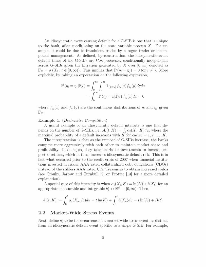
An idiosyncratic event causing default for a G-SIB is one that is uniqueto the bank, after conditioning on the state variable process X. For ex-ample, it could be due to fraudulent trades by a rogue trader or incom-petent management. As defined, by construction, the idiosyncratic eventdefault times of the G-SIBs are Cox processes, conditionally independentacross G-SIBs given the filtration generated by X over [0,∞) denoted asFX = σ (Xt : t ∈ [0,∞)). This implies that P (ηi = ηj) = 0 for i 6= j. Moreexplicitly, by taking an expectation on the following expression,
P (ηi = ηj|FX) =
ˆ ∞
0
ˆ ∞
0
1x=yfηi(x)fηj (y)dydx
=
ˆ ∞
0
P (ηj = x|FX) fηi(x)dx = 0
where fηi(x) and fηj (y) are the continuous distributions of ηi and ηj givenFX .
Example 1. (Destructive Competition)A useful example of an idiosyncratic default intensity is one that de-
pends on the number of G-SIBs, i.e. Ai(t,K) :=´ t
0αi(Xu, K)du, where the
marginal probability of a default increases with K for each i = 1, 2, . . . , K.The interpretation is that as the number of G-SIBs increase, the banks
compete more aggressively with each other to maintain market share andprofitability. In doing so, they take on riskier investments to increase ex-pected returns, which in turn, increases idiosyncratic default risk. This is infact what occurred prior to the credit crisis of 2007 when financial institu-tions invested in riskier AAA rated collateralized debt obligations (CDOs)instead of the riskless AAA rated U.S. Treasuries to obtain increased yields(see Crouhy, Jarrow and Turnbull [9] or Protter [13] for a more detailedexplanation).
A special case of this intensity is when αi(Xt, K) = ln(K)+ b(Xt) for anappropriate measurable and integrable b(·) : Rd → [0,∞). Then,
Ai(t,K) :=
ˆ t
0
αi(Xu, K)du = t ln(K) +
ˆ t
0
b(Xu)du = t ln(K) +B(t).
2.2 Market-Wide Stress Events
Next, define η0 to be the occurrence of a market-wide stress event, as distinctfrom an idiosyncratic default event specific to a single G-SIB. For example,
5
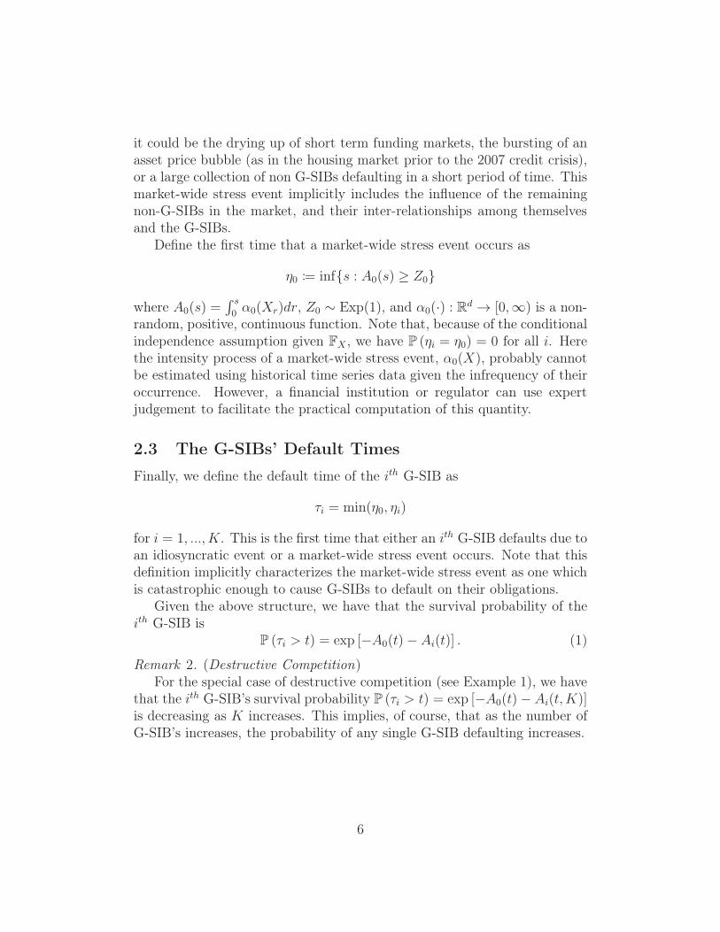
it could be the drying up of short term funding markets, the bursting of anasset price bubble (as in the housing market prior to the 2007 credit crisis),or a large collection of non G-SIBs defaulting in a short period of time. Thismarket-wide stress event implicitly includes the influence of the remainingnon-G-SIBs in the market, and their inter-relationships among themselvesand the G-SIBs.
Define the first time that a market-wide stress event occurs as
η0 := infs : A0(s) ≥ Z0
where A0(s) =´ s
0α0(Xr)dr, Z0 ∼ Exp(1), and α0(·) : Rd → [0,∞) is a non-
random, positive, continuous function. Note that, because of the conditionalindependence assumption given FX , we have P (ηi = η0) = 0 for all i. Herethe intensity process of a market-wide stress event, α0(X), probably cannotbe estimated using historical time series data given the infrequency of theiroccurrence. However, a financial institution or regulator can use expertjudgement to facilitate the practical computation of this quantity.
2.3 The G-SIBs’ Default Times
Finally, we define the default time of the ith G-SIB as
τi = min(η0, ηi)
for i = 1, ..., K. This is the first time that either an ith G-SIB defaults due toan idiosyncratic event or a market-wide stress event occurs. Note that thisdefinition implicitly characterizes the market-wide stress event as one whichis catastrophic enough to cause G-SIBs to default on their obligations.
Given the above structure, we have that the survival probability of theith G-SIB is
P (τi > t) = exp [−A0(t)− Ai(t)] . (1)
Remark 2. (Destructive Competition)For the special case of destructive competition (see Example 1), we have
that the ith G-SIB’s survival probability P (τi > t) = exp [−A0(t)− Ai(t,K)]is decreasing as K increases. This implies, of course, that as the number ofG-SIB’s increases, the probability of any single G-SIB defaulting increases.
6
2.4 The Market Failure Time
We now can define a financial market failure. To fix the intuition, as aninitial attempt, we first define a financial market failure as the event
ω ∈ Ω : τi = τj for some (i, j) ∈ (1, ..., K)× (1, ..., K) , i 6= j ,
and the probability of a financial market failure, our systemic risk measure,as
P (τi = τj for some (i, j) ∈ (1, ..., K)× (1, ..., K) , i 6= j) .
This is the probability that two G-SIBs default at the exactly the same time.The idea underlying this market-failure probability is that if one G-SIB fails,regulators can manage the resulting failure to ensure that a market-widefailure does not occur. However, if two (or more) G-SIBs fail at the sametime, then such an event is uncontrollable by the regulators, resulting in amarket-wide failure.
Unfortunately, there is a problem with this initial systemic risk measure.Given the definition of the ith G-SIB’s default time τi and the conditionalindependence assumption given FX across ηi for i = 0, 1, ..., K, a marketfailure occurs under this definition with probability one if and only if η0 ≤ ηiand η0 ≤ ηj for some pair i 6= j. This is because P (ηi = ηj) = 0 for i 6= j,(i, j) ∈ (1, ..., K)× (1, ..., K). In essence, a market failure only occurs underthis definition, in probability, when a market-wide stress event occurs. Inprobability, the existence of G-SIBs is irrelevant to this initial systemic riskmeasure. To remove this problem, we generalize the definition of a financialmarket failure event to be
ω ∈ Ω : |τi − τj| < ε for some (i, j) ∈ (1, ..., K)× (1, ..., K) , i 6= j
for a given ε > 0, and our (final) systemic risk measure as
P (|τi − τj | < ε for some (i, j) ∈ (1, ..., K)× (1, ..., K) , i 6= j) .
Under this systemic risk measure, a market failure can occur for two reasons:a market-wide stress event occurs, or two G-SIBs experience idiosyncraticdefault events within an ε time period of each other. The next sectioncharacterizes this market-wide default probability.
3 Theorems
This section provides the key theorems characterizing the probability distri-bution of defaults times for the various G-SIBs (“banks”) and the probability
7
of a market failure.
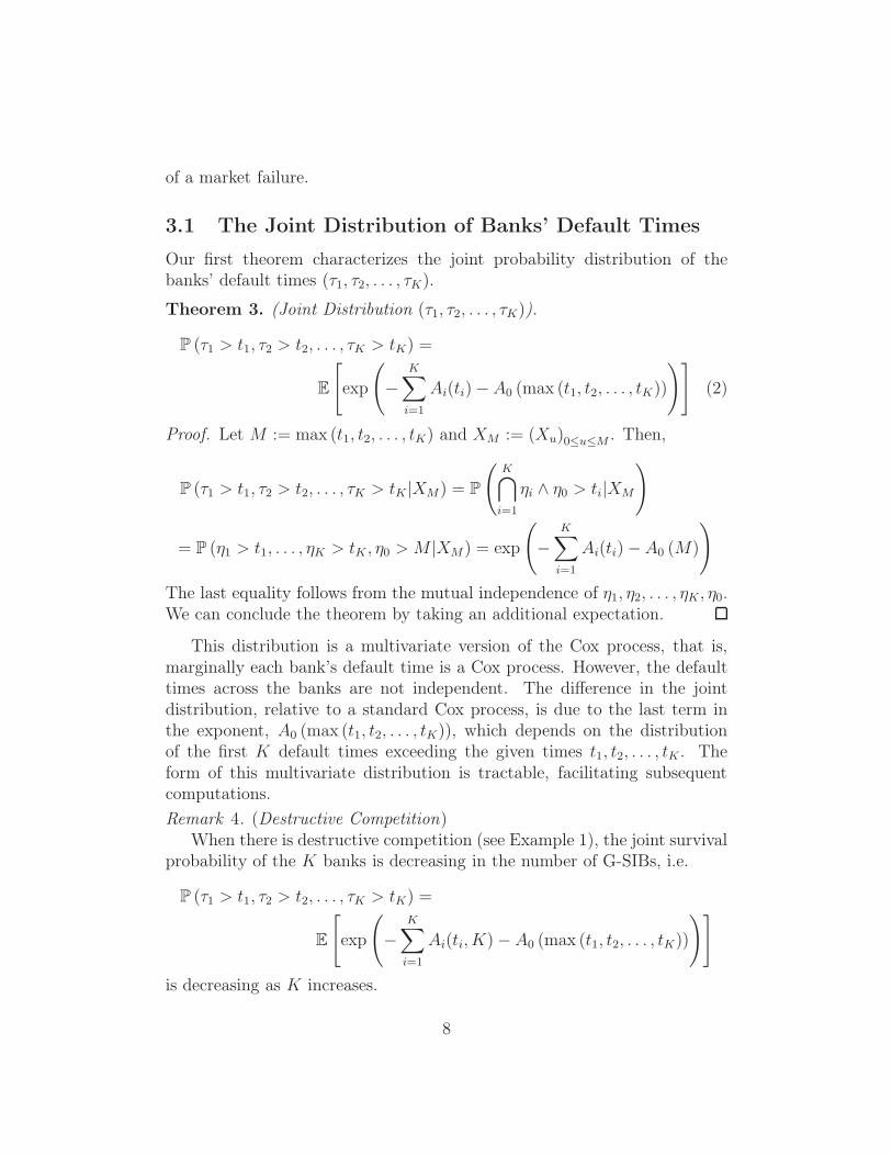
3.1 The Joint Distribution of Banks’ Default Times
Our first theorem characterizes the joint probability distribution of thebanks’ default times (τ1, τ2, . . . , τK).
Theorem 3. (Joint Distribution (τ1, τ2, . . . , τK)).
P (τ1 > t1, τ2 > t2, . . . , τK > tK) =
E
[
exp
(
−
K∑
i=1
Ai(ti)−A0 (max (t1, t2, . . . , tK))
)]
(2)
Proof. Let M := max (t1, t2, . . . , tK) and XM := (Xu)0≤u≤M . Then,
P (τ1 > t1, τ2 > t2, . . . , τK > tK |XM) = P
(
K⋂
i=1
ηi ∧ η0 > ti|XM
)
= P (η1 > t1, . . . , ηK > tK , η0 > M |XM ) = exp
(
−
K∑
i=1
Ai(ti)−A0 (M)
)
The last equality follows from the mutual independence of η1, η2, . . . , ηK , η0.We can conclude the theorem by taking an additional expectation.
This distribution is a multivariate version of the Cox process, that is,marginally each bank’s default time is a Cox process. However, the defaulttimes across the banks are not independent. The difference in the jointdistribution, relative to a standard Cox process, is due to the last term inthe exponent, A0 (max (t1, t2, . . . , tK)), which depends on the distributionof the first K default times exceeding the given times t1, t2, . . . , tK . Theform of this multivariate distribution is tractable, facilitating subsequentcomputations.
Remark 4. (Destructive Competition)When there is destructive competition (see Example 1), the joint survival
probability of the K banks is decreasing in the number of G-SIBs, i.e.
P (τ1 > t1, τ2 > t2, . . . , τK > tK) =
E
[
exp
(
−K∑
i=1
Ai(ti, K)− A0 (max (t1, t2, . . . , tK))
)]
is decreasing as K increases.
8
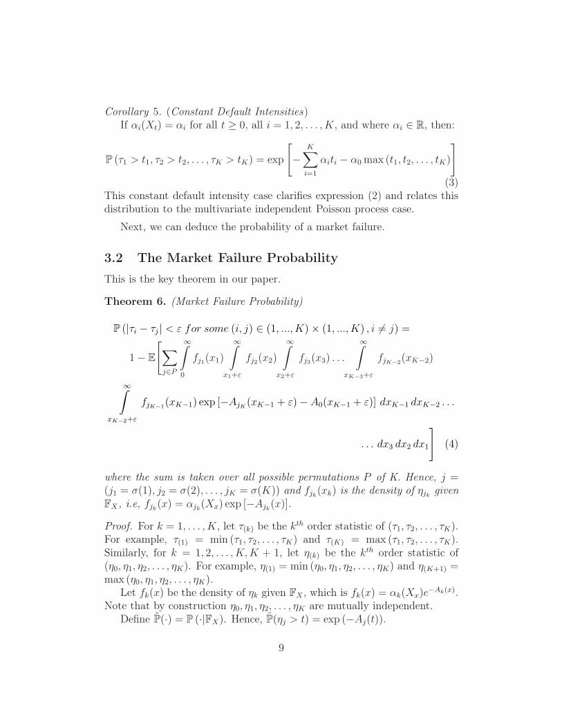
Corollary 5. (Constant Default Intensities)If αi(Xt) = αi for all t ≥ 0, all i = 1, 2, . . . , K, and where αi ∈ R, then:
P (τ1 > t1, τ2 > t2, . . . , τK > tK) = exp
[
−
K∑
i=1
αiti − α0max (t1, t2, . . . , tK)
]
(3)This constant default intensity case clarifies expression (2) and relates thisdistribution to the multivariate independent Poisson process case.
Next, we can deduce the probability of a market failure.
3.2 The Market Failure Probability
This is the key theorem in our paper.
Theorem 6. (Market Failure Probability)
P (|τi − τj | < ε for some (i, j) ∈ (1, ..., K)× (1, ..., K) , i 6= j) =
1− E
[
∑
j∈P
∞
0
fj1(x1)
∞
x1+ε
fj2(x2)
∞
x2+ε
fj3(x3) . . .
∞
xK−3+ε
fjK−2(xK−2)
∞
xK−2+ε
fjK−1(xK−1) exp [−AjK (xK−1 + ε)−A0(xK−1 + ε)] dxK−1 dxK−2 . . .
. . . dx3 dx2 dx1
]
(4)
where the sum is taken over all possible permutations P of K. Hence, j =(j1 = σ(1), j2 = σ(2), . . . , jK = σ(K)) and fjk(xk) is the density of ηjk givenFX , i.e, fjk(x) = αjk(Xx) exp [−Ajk(x)].
Proof. For k = 1, . . . , K, let τ(k) be the kth order statistic of (τ1, τ2, . . . , τK).For example, τ(1) = min (τ1, τ2, . . . , τK) and τ(K) = max (τ1, τ2, . . . , τK).Similarly, for k = 1, 2, . . . , K,K + 1, let η(k) be the kth order statistic of(η0, η1, η2, . . . , ηK). For example, η(1) = min (η0, η1, η2, . . . , ηK) and η(K+1) =max (η0, η1, η2, . . . , ηK).
Let fk(x) be the density of ηk given FX , which is fk(x) = αk(Xx)e−Ak(x).
Note that by construction η0, η1, η2, . . . , ηK are mutually independent.Define P(·) = P (·|FX). Hence, P(ηj > t) = exp (−Aj(t)).
9
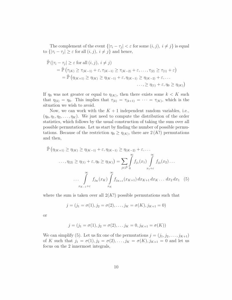
The complement of the event |τi − τj | < ε for some (i, j), i 6= j is equalto |τi − τj | ≥ ε for all (i, j), i 6= j and hence,
P (|τi − τj | ≥ ε for all (i, j), i 6= j)
= P(
τ(K) ≥ τ(K−1) + ε, τ(K−1) ≥ τ(K−2) + ε, . . . , τ(2) ≥ τ(1) + ε)
= P(
η(K+1) ≥ η(K) ≥ η(K−1) + ε, η(K−1) ≥ η(K−2) + ε, . . .
. . . ,≥ η(1) + ε, η0 ≥ η(K)
)
If η0 was not greater or equal to η(K), then there exists some k < K suchthat η(k) = η0. This implies that τ(k) = τ(k+1) = · · · = τ(K), which is thesituation we wish to avoid.
Now, we can work with the K + 1 independent random variables, i.e.,(η0, η1, η2, . . . , ηK). We just need to compute the distribution of the orderstatistics, which follows by the usual construction of taking the sum over allpossible permutations. Let us start by finding the number of possible permu-tations. Because of the restriction η0 ≥ η(K), there are 2 (K!) permutationsand then,
P(
η(K+1) ≥ η(K) ≥ η(K−1) + ε, η(K−1) ≥ η(K−2) + ε, . . .
. . . , η(2) ≥ η(1) + ε, η0 ≥ η(K)
)
=∑
j∈P
∞
0
fj1(x1)
∞
x1+ε
fj2(x2) . . .
. . .
∞
xK−1+ε
fjK(xK)
∞
xK
fjK+1(xK+1) dxK+1 dxK . . . dx2 dx1 (5)
where the sum is taken over all 2(K!) possible permutations such that
j = (j1 = σ(1), j2 = σ(2), . . . , jK = σ(K), jK+1 = 0)
or
j = (j1 = σ(1), j2 = σ(2), . . . jK = 0, jK+1 = σ(K))
We can simplify (5). Let us fix one of the permutations j = (j1, j2, . . . , jK+1)of K such that j1 = σ(1), j2 = σ(2), . . . , jK = σ(K), jK+1 = 0 and let usfocus on the 2 innermost integrals,
10
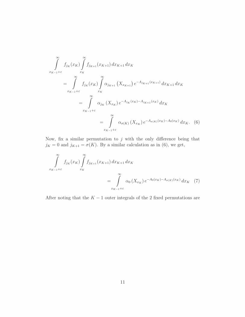
∞
xK−1+ε
fjK (xK)
∞
xK
fjK+1(xK+1) dxK+1 dxK
=
∞
xK−1+ε
fjK(xK)
∞
xK
αjK+1
(
XxK+1
)
e−AjK+1(xK+1) dxK+1 dxK
=
∞
xK−1+ε
αjK (XxK) e−AjK
(xK)−AjK+1(xK) dxK
=
∞
xK−1+ε
ασ(K) (XxK) e−Aσ(K)(xK)−A0(xK) dxK . (6)
Now, fix a similar permutation to j with the only difference being thatjK = 0 and jK+1 = σ(K). By a similar calculation as in (6), we get,
∞
xK−1+ε
fjK (xK)
∞
xK
fjK+1(xK+1) dxK+1 dxK
=
∞
xK−1+ε
α0 (XxK) e−A0(xK)−Aσ(K)(xK) dxK (7)
After noting that the K − 1 outer integrals of the 2 fixed permutations are
11
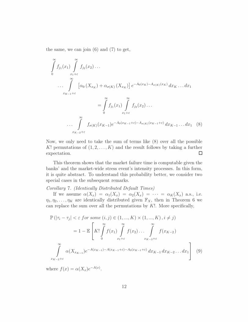
the same, we can join (6) and (7) to get,
∞
0
fj1(x1)
∞
x1+ε
fj2(x2) . . .
. . .
∞
xK−1+ε
[
α0 (XxK) + ασ(K) (XxK
)]
e−A0(xK)−Aσ(K)(xK) dxK . . . dx1
=
∞
0
fj1(x1)
∞
x1+ε
fj2(x2) . . .
. . .
∞
xK−2+ε
fσ(K)(xK−1)e−A0(xK−1+ε)−Aσ(K)(xK−1+ε) dxK−1 . . . dx1 (8)
Now, we only need to take the sum of terms like (8) over all the possibleK! permutations of (1, 2, . . . , K) and the result follows by taking a furtherexpectation.
This theorem shows that the market failure time is computable given thebanks’ and the market-wide stress event’s intensity processes. In this form,it is quite abstract. To understand this probability better, we consider twospecial cases in the subsequent remarks.
Corollary 7. (Identically Distributed Default Times)If we assume α(Xx) = α1(Xx) = α2(Xx) = · · · = αK(Xx) a.s., i.e.
η1, η2, . . . , ηK are identically distributed given FX , then in Theorem 6 wecan replace the sum over all the permutations by K!. More specifically,
P (|τi − τj | < ε for some (i, j) ∈ (1, ..., K)× (1, ..., K) , i 6= j)
= 1− E
K!
∞
0
f(x1)
∞
x1+ε
f(x2) . . .
∞
xK−3+ε
f(xK−2 )
∞
xK−2+ε
α(XxK−1)e−A(xK−1)−A(xK−1+ε)−A0(xK−1+ε) dxK−1 dxK−2 . . . dx1
(9)
where f(x) = α(Xx)e−A(x).
12
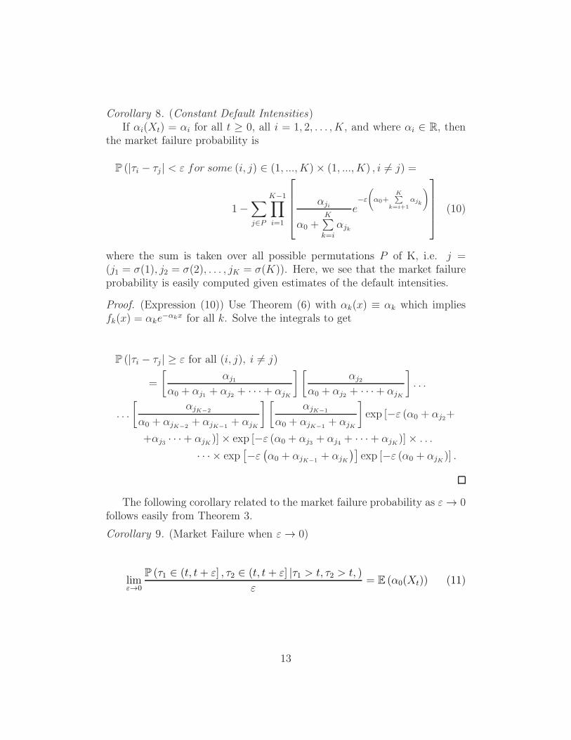
Corollary 8. (Constant Default Intensities)If αi(Xt) = αi for all t ≥ 0, all i = 1, 2, . . . , K, and where αi ∈ R, then
the market failure probability is
P (|τi − τj | < ε for some (i, j) ∈ (1, ..., K)× (1, ..., K) , i 6= j) =
1−∑
j∈P
K−1∏
i=1
αji
α0 +K∑
k=i
αjk
e−ε
(
α0+K∑
k=i+1αjk
)
(10)
where the sum is taken over all possible permutations P of K, i.e. j =(j1 = σ(1), j2 = σ(2), . . . , jK = σ(K)). Here, we see that the market failureprobability is easily computed given estimates of the default intensities.
Proof. (Expression (10)) Use Theorem (6) with αk(x) ≡ αk which impliesfk(x) = αke
−αkx for all k. Solve the integrals to get
P (|τi − τj | ≥ ε for all (i, j), i 6= j)
=
[
αj1
α0 + αj1 + αj2 + · · ·+ αjK
] [
αj2
α0 + αj2 + · · ·+ αjK
]
. . .
. . .
[
αjK−2
α0 + αjK−2+ αjK−1
+ αjK
] [
αjK−1
α0 + αjK−1+ αjK
]
exp [−ε (α0 + αj2+
+αj3 · · ·+ αjK )]× exp [−ε (α0 + αj3 + αj4 + · · ·+ αjK)]× . . .
· · · × exp[
−ε(
α0 + αjK−1+ αjK
)]
exp [−ε (α0 + αjK)] .
The following corollary related to the market failure probability as ε → 0follows easily from Theorem 3.
Corollary 9. (Market Failure when ε → 0)
limε→0
P (τ1 ∈ (t, t+ ε] , τ2 ∈ (t, t + ε] |τ1 > t, τ2 > t, )
ε= E (α0(Xt)) (11)
13
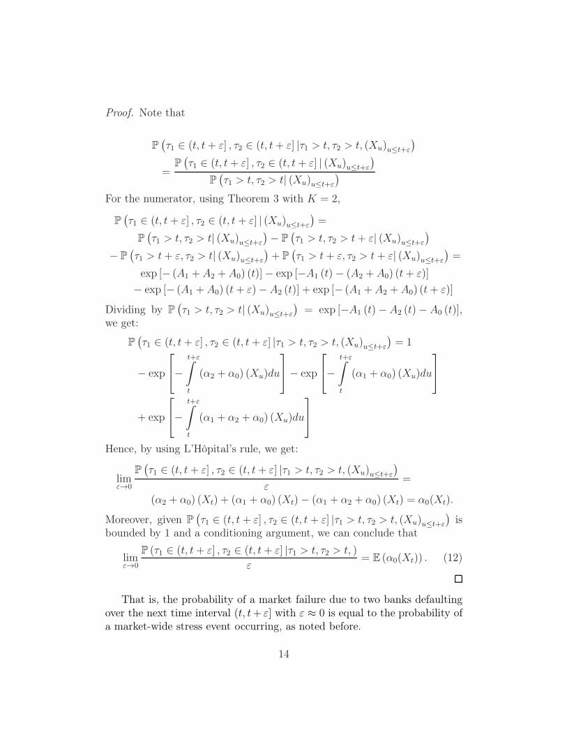
Proof. Note that
P(
τ1 ∈ (t, t+ ε] , τ2 ∈ (t, t+ ε] |τ1 > t, τ2 > t, (Xu)u≤t+ε
)
=P(
τ1 ∈ (t, t+ ε] , τ2 ∈ (t, t+ ε] | (Xu)u≤t+ε
)
P(
τ1 > t, τ2 > t| (Xu)u≤t+ε
)
For the numerator, using Theorem 3 with K = 2,
P(
τ1 ∈ (t, t+ ε] , τ2 ∈ (t, t + ε] | (Xu)u≤t+ε
)
=
P(
τ1 > t, τ2 > t| (Xu)u≤t+ε
)
− P(
τ1 > t, τ2 > t+ ε| (Xu)u≤t+ε
)
− P(
τ1 > t+ ε, τ2 > t| (Xu)u≤t+ε
)
+ P(
τ1 > t + ε, τ2 > t + ε| (Xu)u≤t+ε
)
=
exp [− (A1 + A2 + A0) (t)]− exp [−A1 (t)− (A2 + A0) (t+ ε)]
− exp [− (A1 + A0) (t+ ε)−A2 (t)] + exp [− (A1 + A2 + A0) (t+ ε)]
Dividing by P(
τ1 > t, τ2 > t| (Xu)u≤t+ε
)
= exp [−A1 (t)− A2 (t)− A0 (t)],we get:
P(
τ1 ∈ (t, t+ ε] , τ2 ∈ (t, t+ ε] |τ1 > t, τ2 > t, (Xu)u≤t+ε
)
= 1
− exp
−
t+εˆ
t
(α2 + α0) (Xu)du
− exp
−
t+εˆ
t
(α1 + α0) (Xu)du
+ exp
−
t+εˆ
t
(α1 + α2 + α0) (Xu)du
Hence, by using L’Hôpital’s rule, we get:
limε→0
P(
τ1 ∈ (t, t+ ε] , τ2 ∈ (t, t+ ε] |τ1 > t, τ2 > t, (Xu)u≤t+ε
)
ε=
(α2 + α0) (Xt) + (α1 + α0) (Xt)− (α1 + α2 + α0) (Xt) = α0(Xt).
Moreover, given P(
τ1 ∈ (t, t + ε] , τ2 ∈ (t, t + ε] |τ1 > t, τ2 > t, (Xu)u≤t+ε
)
isbounded by 1 and a conditioning argument, we can conclude that
limε→0
P (τ1 ∈ (t, t+ ε] , τ2 ∈ (t, t+ ε] |τ1 > t, τ2 > t, )
ε= E (α0(Xt)) . (12)
That is, the probability of a market failure due to two banks defaultingover the next time interval (t, t+ ε] with ε ≈ 0 is equal to the probability ofa market-wide stress event occurring, as noted before.
14
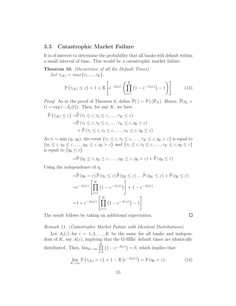
3.3 Catastrophic Market Failure
It is of interest to determine the probability that all banks will default withina small interval of time. This would be a catastrophic market failure.
Theorem 10. (Occurrence of all the Default Times)Let τ(K) = maxτ1, ..., τK.
P(
τ(K) ≤ ε)
= 1 + E
[
e−A0(ε)
(
K∏
i=1
(
1− e−Ai(ε))
− 1
)]
(13)
Proof. As in the proof of Theorem 6, define P(·) = P (·|FX). Hence, P(ηj >t) = exp (−Aj(t)). Then, for any K, we have
P(
τ(K) ≤ ε)
=P (τ1 ≤ ε, τ2 ≤ ε, . . . , τK ≤ ε)
=P (τ1 ≤ ε, τ2 ≤ ε, . . . , τK ≤ ε, η0 > ε)
+ P (τ1 ≤ ε, τ2 ≤ ε, . . . , τK ≤ ε, η0 ≤ ε)
As τi = min (ηi, η0), the event τ1 ≤ ε, τ2 ≤ ε, . . . , τK ≤ ε, η0 > ε is equal toη1 ≤ ε, η2 ≤ ε, . . . , ηK ≤ ε, η0 > ε and τ1 ≤ ε, τ2 ≤ ε, . . . , τK ≤ ε, η0 ≤ εis equal to η0 ≤ ǫ
=P (η1 ≤ ε, η2 ≤ ε, . . . , ηK ≤ ε, η0 > ε) + P (η0 ≤ ε)
Using the independence of ηi
=P (η0 > ε) P (η1 ≤ ε) P (η2 ≤ ε) . . . P (ηK ≤ ε) + P (η0 ≤ ε)
=e−A0(ε)
[
K∏
i=1
(
1− e−Ai(ε))
]
+ 1− e−A0(ε)
=1 + e−A0(ε)
[
K∏
i=1
(
1− e−Ai(ε))
− 1
]
The result follows by taking an additional expectation.
Remark 11. (Catastrophic Market Failure with Identical Distributions)
Let Ai(ε) for i = 1, 2, . . . , K be the same for all banks and indepen-dent of K, say A(ε), implying that the G-SIBs’ default times are identically
distributed. Then, limK→∞
K∏
i=1
(
1− e−A(ε))
= 0, which implies that
limK→∞
P(
τ(K) < ε)
= 1− E(
e−A0(ε))
= P (η0 < ε) . (14)
15
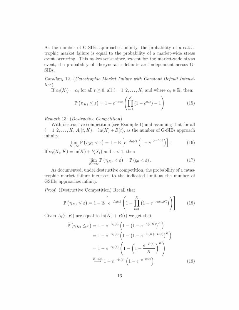
As the number of G-SIBs approaches infinity, the probability of a catas-trophic market failure is equal to the probability of a market-wide stressevent occurring. This makes sense since, except for the market-wide stressevent, the probability of idiosyncratic defaults are independent across G-SIBs.
Corollary 12. (Catastrophic Market Failure with Constant Default Intensi-ties)
If αi(Xt) = αi for all t ≥ 0, all i = 1, 2, . . . , K, and where αi ∈ R, then:
P(
τ(K) ≤ ε)
= 1 + e−α0ε
(
K∏
i=1
(1− eαiε)− 1
)
(15)
Remark 13. (Destructive Competition)With destructive competition (see Example 1) and assuming that for all
i = 1, 2, . . . , K, Ai(t,K) = ln(K)+B(t), as the number of G-SIBs approachinfinity,
limK→∞
P(
τ(K) < ε)
= 1− E[
e−A0(ε)(
1− e−e−B(ε))]
. (16)
If αi(Xt, K) = ln(K) + b(Xt) and ε < 1, then
limK→∞
P(
τ(K) < ε)
= P (η0 < ε) . (17)
As documented, under destructive competition, the probability of a catas-trophic market failure increases to the indicated limit as the number ofGSIBs approaches infinity.
Proof. (Destructive Competition) Recall that
P(
τ(K) ≤ ε)
= 1− E
[
e−A0(ε)
(
1−
K∏
i=1
(
1− e−Ai(ε,K))
)]
(18)
Given Ai(ε,K) are equal to ln(K) +B(t) we get that
P(
τ(K) ≤ ε)
= 1− e−A0(ε)(
1−(
1− e−A(ε,K))K)
= 1− e−A0(ε)(
1−(
1− e− ln(K)−B(ε))K)
= 1− e−A0(ε)
(
1−
(
1−e−B(ε)
K
)K)
K→∞−→ 1− e−A0(ε)
(
1− e−e−B(ε))
(19)
16
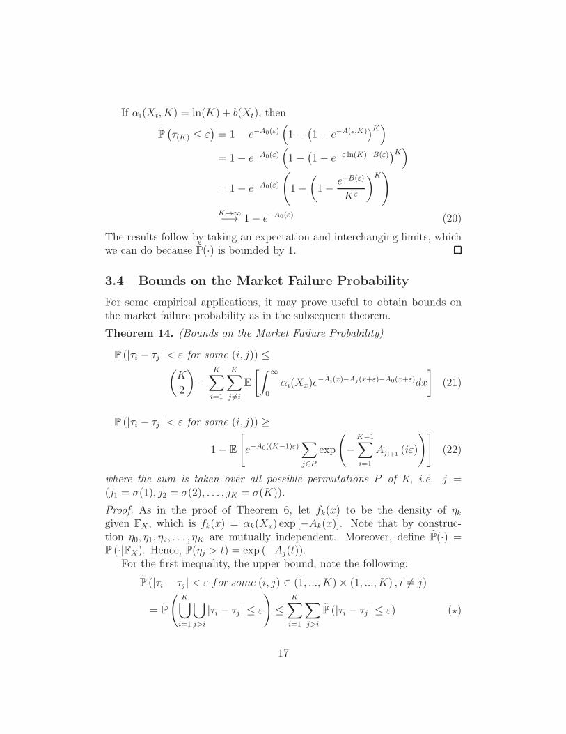
If αi(Xt, K) = ln(K) + b(Xt), then
P(
τ(K) ≤ ε)
= 1− e−A0(ε)(
1−(
1− e−A(ε,K))K)
= 1− e−A0(ε)(
1−(
1− e−ε ln(K)−B(ε))K)
= 1− e−A0(ε)
(
1−
(
1−e−B(ε)
Kε
)K)
K→∞−→ 1− e−A0(ε) (20)
The results follow by taking an expectation and interchanging limits, whichwe can do because P(·) is bounded by 1.
3.4 Bounds on the Market Failure Probability
For some empirical applications, it may prove useful to obtain bounds onthe market failure probability as in the subsequent theorem.
Theorem 14. (Bounds on the Market Failure Probability)
P (|τi − τj | < ε for some (i, j)) ≤(
K
2
)
−K∑
i=1
K∑
j 6=i
E
[ˆ ∞
0
αi(Xx)e−Ai(x)−Aj(x+ε)−A0(x+ε)dx
]
(21)
P (|τi − τj | < ε for some (i, j)) ≥
1− E
[
e−A0((K−1)ε)∑
j∈P
exp
(
−
K−1∑
i=1
Aji+1(iε)
)]
(22)
where the sum is taken over all possible permutations P of K, i.e. j =(j1 = σ(1), j2 = σ(2), . . . , jK = σ(K)).
Proof. As in the proof of Theorem 6, let fk(x) to be the density of ηkgiven FX , which is fk(x) = αk(Xx) exp [−Ak(x)]. Note that by construc-tion η0, η1, η2, . . . , ηK are mutually independent. Moreover, define P(·) =P (·|FX). Hence, P(ηj > t) = exp (−Aj(t)).
For the first inequality, the upper bound, note the following:
P (|τi − τj | < ε for some (i, j) ∈ (1, ..., K)× (1, ..., K) , i 6= j)
= P
(
K⋃
i=1
⋃
j>i
|τi − τj | ≤ ε
)
≤
K∑
i=1
∑
j>i
P (|τi − τj | ≤ ε) (⋆)
17
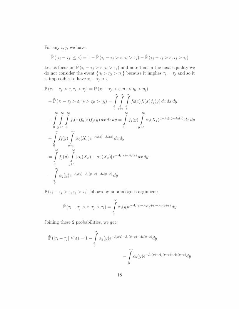
For any i, j, we have:
P (|τi − τj | ≤ ε) = 1− P (τi − τj > ε, τi > τj)− P (τj − τi > ε, τj > τi)
Let us focus on P (τi − τj > ε, τi > τj) and note that in the next equality wedo not consider the event ηi > ηj > η0 because it implies τi = τj and so itis impossible to have τi − τj > ε
P (τi − τj > ε, τi > τj) = P (τi − τj > ε, η0 > ηi > ηj)
+ P (τi − τj > ε, ηi > η0 > ηj) =
∞
0
∞
y+ε
∞
x
f0(z)fi(x)fj(y) dz dx dy
+
∞
0
∞
y+ε
∞
z
fi(x)f0(z)fj(y) dx dz dy =
∞
0
fj(y)
∞
y+ε
αi(Xx)e−Ai(x)−A0(x) dx dy
+
∞
0
fj(y)
∞
y+ε
α0(Xz)e−Ai(z)−A0(z) dz dy
=
∞
0
fj(y)
∞
y+ε
[αi(Xx) + α0(Xx)] e−Ai(x)−A0(x) dx dy
=
∞
0
αj(y)e−Aj(y)−Ai(y+ε)−A0(y+ε) dy
P (τi − τj > ε, τj > τi) follows by an analogous argument:
P (τi − τj > ε, τj > τi) =
∞
0
αi(y)e−Ai(y)−Aj(y+ε)−A0(y+ε) dy
Joining these 2 probabilities, we get:
P (|τi − τj | ≤ ε) = 1−
∞
0
αj(y)e−Aj(y)−Ai(y+ε)−A0(y+ε)dy
−
∞
0
αi(y)e−Ai(y)−Aj (y+ε)−A0(y+ε)dy
18
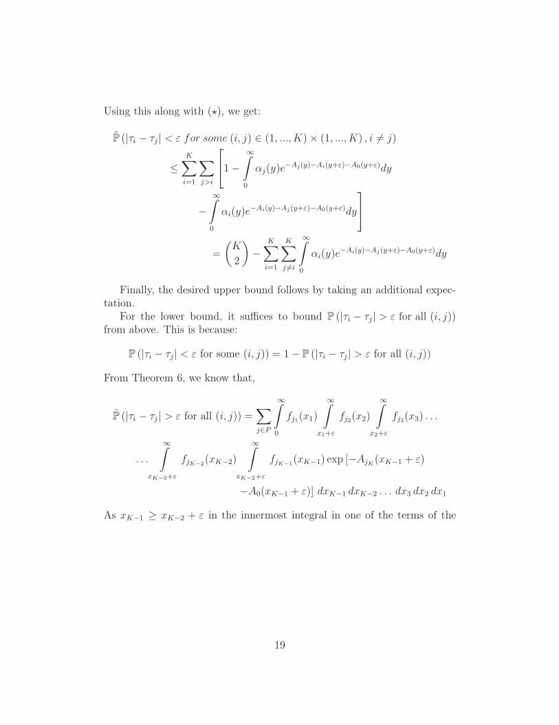
Using this along with (⋆), we get:
P (|τi − τj | < ε for some (i, j) ∈ (1, ..., K)× (1, ..., K) , i 6= j)
≤
K∑
i=1
∑
j>i
1−
∞
0
αj(y)e−Aj(y)−Ai(y+ε)−A0(y+ε)dy
−
∞
0
αi(y)e−Ai(y)−Aj(y+ε)−A0(y+ε)dy
=
(
K
2
)
−
K∑
i=1
K∑
j 6=i
∞
0
αi(y)e−Ai(y)−Aj (y+ε)−A0(y+ε)dy
Finally, the desired upper bound follows by taking an additional expec-tation.
For the lower bound, it suffices to bound P (|τi − τj | > ε for all (i, j))from above. This is because:
P (|τi − τj| < ε for some (i, j)) = 1− P (|τi − τj | > ε for all (i, j))
From Theorem 6, we know that,
P (|τi − τj | > ε for all (i, j)) =∑
j∈P
∞
0
fj1(x1)
∞
x1+ε
fj2(x2)
∞
x2+ε
fj3(x3) . . .
. . .
∞
xK−3+ε
fjK−2(xK−2)
∞
xK−2+ε
fjK−1(xK−1) exp [−AjK (xK−1 + ε)
−A0(xK−1 + ε)] dxK−1 dxK−2 . . . dx3 dx2 dx1
As xK−1 ≥ xK−2 + ε in the innermost integral in one of the terms of the
19
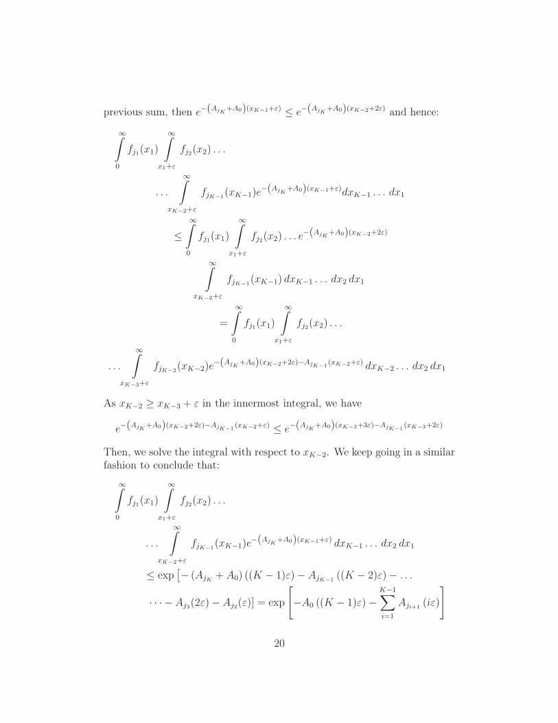
previous sum, then e−(AjK+A0)(xK−1+ε) ≤ e−(AjK
+A0)(xK−2+2ε) and hence:
∞
0
fj1(x1)
∞
x1+ε
fj2(x2) . . .
. . .
∞
xK−2+ε
fjK−1(xK−1)e
−(AjK+A0)(xK−1+ε)dxK−1 . . . dx1
≤
∞
0
fj1(x1)
∞
x1+ε
fj2(x2) . . . e−(AjK
+A0)(xK−2+2ε)
∞
xK−2+ε
fjK−1(xK−1) dxK−1 . . . dx2 dx1
=
∞
0
fj1(x1)
∞
x1+ε
fj2(x2) . . .
. . .
∞
xK−3+ε
fjK−2(xK−2)e
−(AjK+A0)(xK−2+2ε)−AjK−1
(xK−2+ε) dxK−2 . . . dx2 dx1
As xK−2 ≥ xK−3 + ε in the innermost integral, we have
e−(AjK+A0)(xK−2+2ε)−AjK−1
(xK−2+ε) ≤ e−(AjK+A0)(xK−3+3ε)−AjK−1
(xK−3+2ε)
Then, we solve the integral with respect to xK−2. We keep going in a similarfashion to conclude that:
∞
0
fj1(x1)
∞
x1+ε
fj2(x2) . . .
. . .
∞
xK−2+ε
fjK−1(xK−1)e
−(AjK+A0)(xK−1+ε) dxK−1 . . . dx2 dx1
≤ exp[
− (AjK + A0) ((K − 1)ε)− AjK−1((K − 2)ε)− . . .
· · · −Aj3(2ε)− Aj2(ε)] = exp
[
−A0 ((K − 1)ε)−
K−1∑
i=1
Aji+1(iε)
]
20
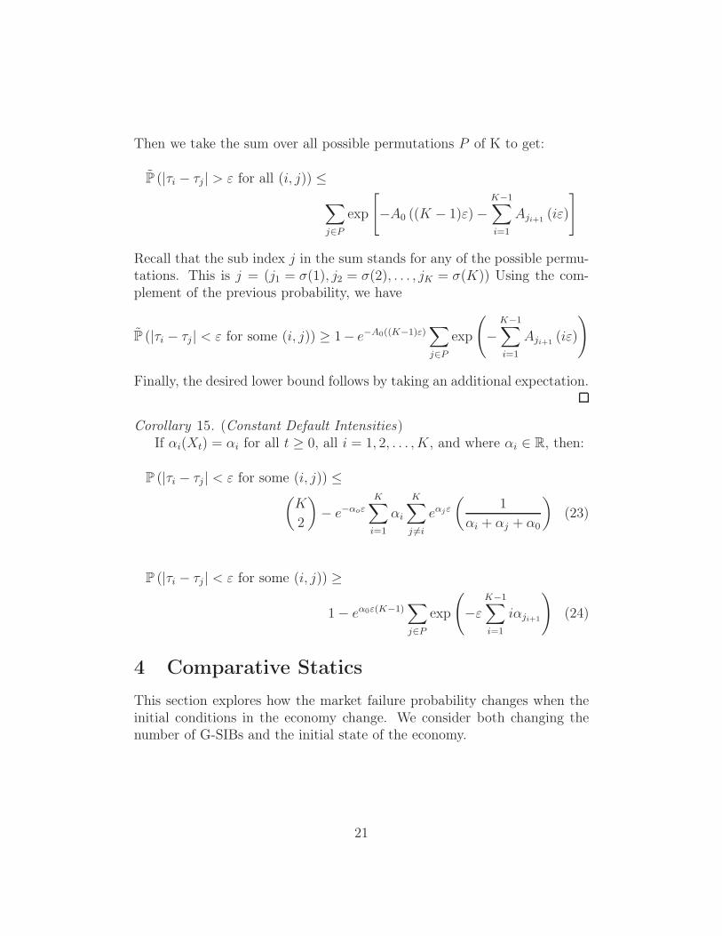
Then we take the sum over all possible permutations P of K to get:
P (|τi − τj | > ε for all (i, j)) ≤
∑
j∈P
exp
[
−A0 ((K − 1)ε)−
K−1∑
i=1
Aji+1(iε)
]
Recall that the sub index j in the sum stands for any of the possible permu-tations. This is j = (j1 = σ(1), j2 = σ(2), . . . , jK = σ(K)) Using the com-plement of the previous probability, we have
P (|τi − τj | < ε for some (i, j)) ≥ 1− e−A0((K−1)ε)∑
j∈P
exp
(
−
K−1∑
i=1
Aji+1(iε)
)
Finally, the desired lower bound follows by taking an additional expectation.
Corollary 15. (Constant Default Intensities)If αi(Xt) = αi for all t ≥ 0, all i = 1, 2, . . . , K, and where αi ∈ R, then:
P (|τi − τj | < ε for some (i, j)) ≤(
K
2
)
− e−αoε
K∑
i=1
αi
K∑
j 6=i
eαjε
(
1
αi + αj + α0
)
(23)
P (|τi − τj | < ε for some (i, j)) ≥
1− eα0ε(K−1)∑
j∈P
exp
(
−ε
K−1∑
i=1
iαji+1
)
(24)
4 Comparative Statics
This section explores how the market failure probability changes when theinitial conditions in the economy change. We consider both changing thenumber of G-SIBs and the initial state of the economy.
21
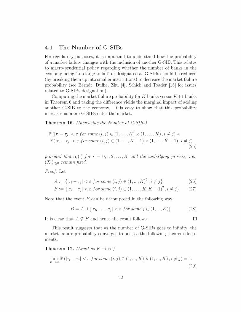
4.1 The Number of G-SIBs
For regulatory purposes, it is important to understand how the probabilityof a market failure changes with the inclusion of another G-SIB. This relatesto macro-prudential policy regarding whether the number of banks in theeconomy being “too large to fail” or designated as G-SIBs should be reduced(by breaking them up into smaller institutions) to decrease the market failureprobability (see Berndt, Duffie, Zhu [4], Schich and Toader [15] for issuesrelated to G-SIBs designation).
Computing the market failure probability for K banks versus K+1 banksin Theorem 6 and taking the difference yields the marginal impact of addinganother G-SIB to the economy. It is easy to show that this probabilityincreases as more G-SIBs enter the market.
Theorem 16. (Increasing the Number of G-SIBs)
P (|τi − τj | < ε for some (i, j) ∈ (1, . . . , K)× (1, . . . , K) , i 6= j) <
P (|τi − τj| < ε for some (i, j) ∈ (1, . . . , K + 1)× (1, . . . , K + 1) , i 6= j)(25)
provided that αi(·) for i = 0, 1, 2, . . . , K and the underlying process, i.e.,(Xt)t≥0 remain fixed.
Proof. Let
A := |τi − τj | < ε for some (i, j) ∈ (1, ..., K)2 , i 6= j (26)
B := |τi − τj | < ε for some (i, j) ∈ (1, . . . , K,K + 1)2 , i 6= j (27)
Note that the event B can be decomposed in the following way:
B = A ∪ |τK+1 − τj | < ε for some j ∈ (1, ..., K) (28)
It is clear that A * B and hence the result follows .
This result suggests that as the number of G-SIBs goes to infinity, themarket failure probability converges to one, as the following theorem docu-ments.
Theorem 17. (Limit as K → ∞)
limK→∞
P (|τi − τj | < ε for some (i, j) ∈ (1, ..., K)× (1, ..., K) , i 6= j) = 1.
(29)
22
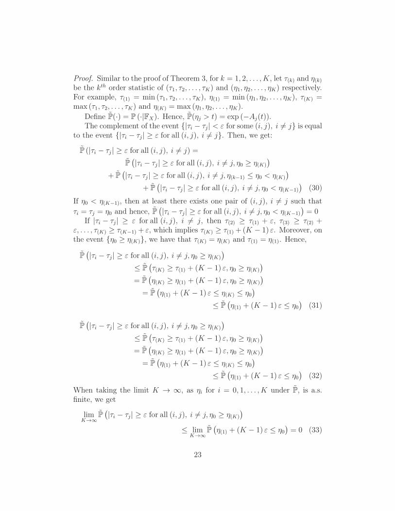
Proof. Similar to the proof of Theorem 3, for k = 1, 2, . . . , K, let τ(k) and η(k)be the kth order statistic of (τ1, τ2, . . . , τK) and (η1, η2, . . . , ηK) respectively.For example, τ(1) = min (τ1, τ2, . . . , τK), η(1) = min (η1, η2, . . . , ηK), τ(K) =max (τ1, τ2, . . . , τK) and η(K) = max (η1, η2, . . . , ηK).
Define P(·) = P (·|FX). Hence, P(ηj > t) = exp (−Aj(t)).The complement of the event |τi − τj | < ε for some (i, j), i 6= j is equal
to the event |τi − τj | ≥ ε for all (i, j), i 6= j. Then, we get:
P (|τi − τj | ≥ ε for all (i, j), i 6= j) =
P(
|τi − τj | ≥ ε for all (i, j), i 6= j, η0 ≥ η(K)
)
+ P(
|τi − τj | ≥ ε for all (i, j), i 6= j, η(k−1) ≤ η0 < η(K)
)
+ P(
|τi − τj | ≥ ε for all (i, j), i 6= j, η0 < η(K−1)
)
(30)
If η0 < η(K−1), then at least there exists one pair of (i, j), i 6= j such that
τi = τj = η0 and hence, P(
|τi − τj| ≥ ε for all (i, j), i 6= j, η0 < η(K−1)
)
= 0If |τi − τj| ≥ ε for all (i, j), i 6= j, then τ(2) ≥ τ(1) + ε, τ(3) ≥ τ(2) +
ε, . . . , τ(K) ≥ τ(K−1) + ε, which implies τ(K) ≥ τ(1) + (K − 1) ε. Moreover, onthe event η0 ≥ η(K), we have that τ(K) = η(K) and τ(1) = η(1). Hence,
P(
|τi − τj | ≥ ε for all (i, j), i 6= j, η0 ≥ η(K)
)
≤ P(
τ(K) ≥ τ(1) + (K − 1) ε, η0 ≥ η(K)
)
= P(
η(K) ≥ η(1) + (K − 1) ε, η0 ≥ η(K)
)
= P(
η(1) + (K − 1) ε ≤ η(K) ≤ η0)
≤ P(
η(1) + (K − 1) ε ≤ η0)
(31)
P(
|τi − τj | ≥ ε for all (i, j), i 6= j, η0 ≥ η(K)
)
≤ P(
τ(K) ≥ τ(1) + (K − 1) ε, η0 ≥ η(K)
)
= P(
η(K) ≥ η(1) + (K − 1) ε, η0 ≥ η(K)
)
= P(
η(1) + (K − 1) ε ≤ η(K) ≤ η0)
≤ P(
η(1) + (K − 1) ε ≤ η0)
(32)
When taking the limit K → ∞, as ηi for i = 0, 1, . . . , K under P, is a.s.finite, we get
limK→∞
P(
|τi − τj| ≥ ε for all (i, j), i 6= j, η0 ≥ η(K)
)
≤ limK→∞
P(
η(1) + (K − 1) ε ≤ η0)
= 0 (33)
23
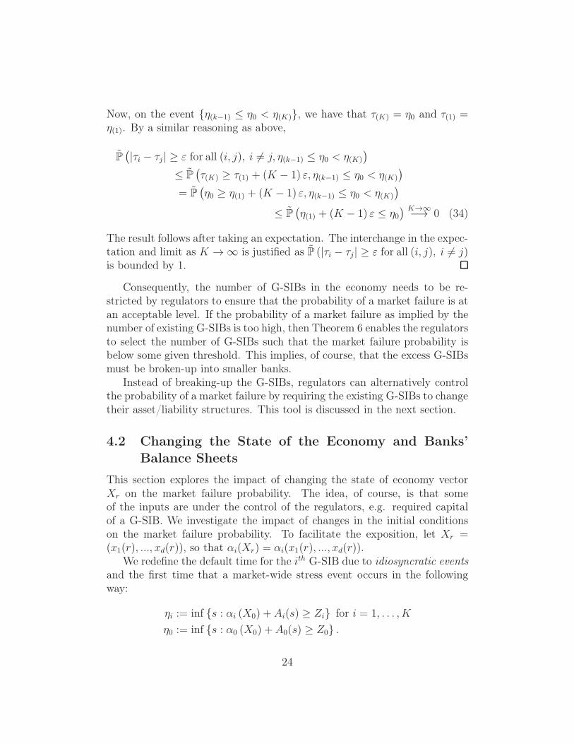
Now, on the event η(k−1) ≤ η0 < η(K), we have that τ(K) = η0 and τ(1) =η(1). By a similar reasoning as above,
P(
|τi − τj | ≥ ε for all (i, j), i 6= j, η(k−1) ≤ η0 < η(K)
)
≤ P(
τ(K) ≥ τ(1) + (K − 1) ε, η(k−1) ≤ η0 < η(K)
)
= P(
η0 ≥ η(1) + (K − 1) ε, η(k−1) ≤ η0 < η(K)
)
≤ P(
η(1) + (K − 1) ε ≤ η0) K→∞−→ 0 (34)
The result follows after taking an expectation. The interchange in the expec-tation and limit as K → ∞ is justified as P (|τi − τj| ≥ ε for all (i, j), i 6= j)is bounded by 1.
Consequently, the number of G-SIBs in the economy needs to be re-stricted by regulators to ensure that the probability of a market failure is atan acceptable level. If the probability of a market failure as implied by thenumber of existing G-SIBs is too high, then Theorem 6 enables the regulatorsto select the number of G-SIBs such that the market failure probability isbelow some given threshold. This implies, of course, that the excess G-SIBsmust be broken-up into smaller banks.
Instead of breaking-up the G-SIBs, regulators can alternatively controlthe probability of a market failure by requiring the existing G-SIBs to changetheir asset/liability structures. This tool is discussed in the next section.
4.2 Changing the State of the Economy and Banks’
Balance Sheets
This section explores the impact of changing the state of economy vectorXr on the market failure probability. The idea, of course, is that someof the inputs are under the control of the regulators, e.g. required capitalof a G-SIB. We investigate the impact of changes in the initial conditionson the market failure probability. To facilitate the exposition, let Xr =(x1(r), ..., xd(r)), so that αi(Xr) = αi(x1(r), ..., xd(r)).
We redefine the default time for the ith G-SIB due to idiosyncratic eventsand the first time that a market-wide stress event occurs in the followingway:
ηi := inf s : αi (X0) + Ai(s) ≥ Zi for i = 1, . . . , K
η0 := inf s : α0 (X0) + A0(s) ≥ Z0 .
24
Just as before, the default time of the ith G-SIB is
τi = min (η0, ηi) .
Then, it is easy to check that
P(
ηi > t| (Xu)0≤u≤t
)
= exp (−αi (X0)−Ai(t))
P(
τi > t| (Xu)0≤u≤t
)
= exp (−αi (X0)− α0 (X0)− Ai(t)− A0(t)) .
To ensure that the probability distributions of ηi and τi are correctly defined,we assign a positive probability to the event ηi = 0 such that
P (ηi = 0|X0) = 1− exp (−αi (X0)) .
This implies that
P (τi = 0|X0) = 1− exp (−αi (X0)− α0 (X0)) .
The interpretation is that there is a positive probability of an “instantaneous”default at t = 0. Under these modifications, we have the following result.
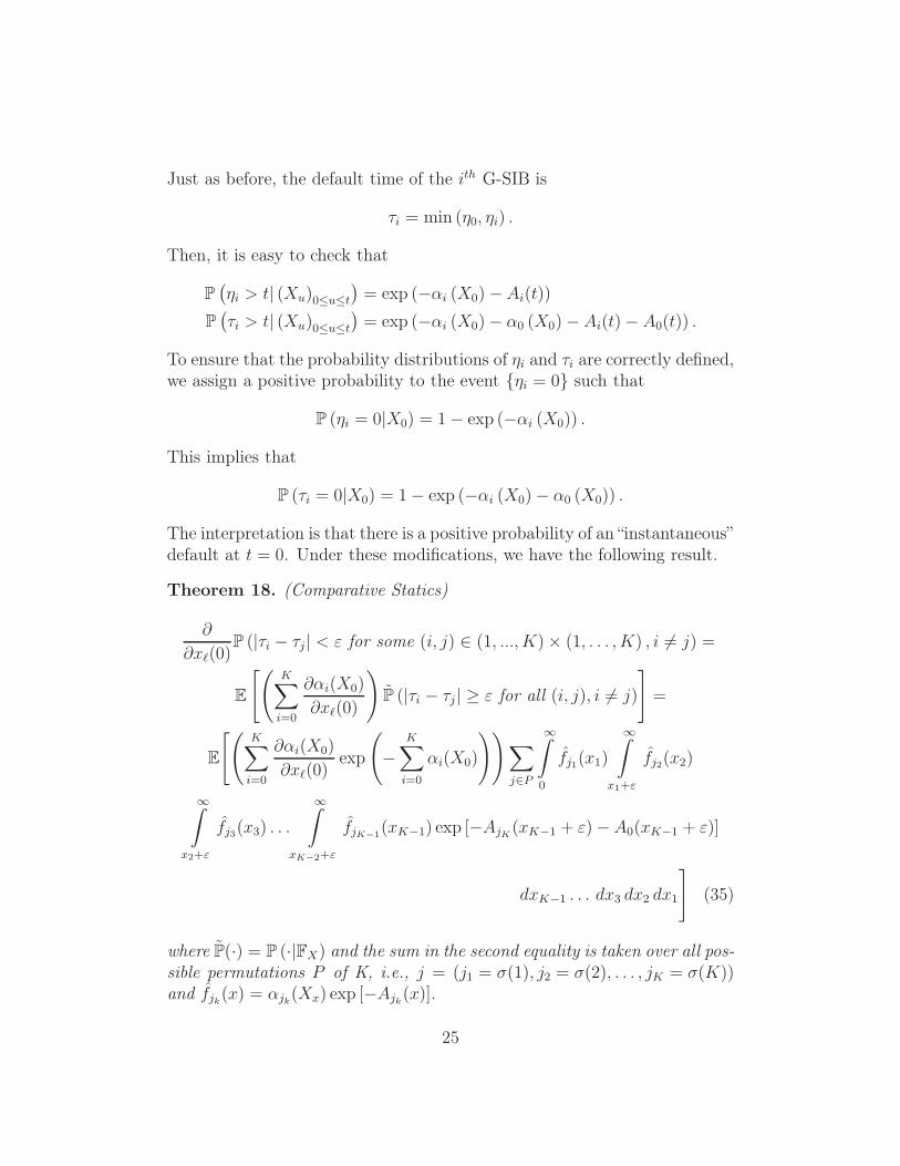
Theorem 18. (Comparative Statics)
∂
∂xℓ(0)P (|τi − τj | < ε for some (i, j) ∈ (1, ..., K)× (1, . . . , K) , i 6= j) =
E
[(
K∑
i=0
∂αi(X0)
∂xℓ(0)
)
P (|τi − τj| ≥ ε for all (i, j), i 6= j)
]
=
E
[(
K∑
i=0
∂αi(X0)
∂xℓ(0)exp
(
−
K∑
i=0
αi(X0)
))
∑
j∈P
∞
0
fj1(x1)
∞
x1+ε
fj2(x2)
∞
x2+ε
fj3(x3) . . .
∞
xK−2+ε
fjK−1(xK−1) exp [−AjK (xK−1 + ε)−A0(xK−1 + ε)]
dxK−1 . . . dx3 dx2 dx1
]
(35)
where P(·) = P (·|FX) and the sum in the second equality is taken over all pos-sible permutations P of K, i.e., j = (j1 = σ(1), j2 = σ(2), . . . , jK = σ(K))and fjk(x) = αjk(Xx) exp [−Ajk(x)].
25
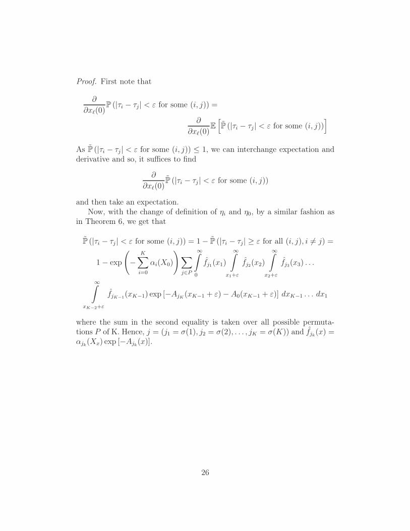
Proof. First note that
∂
∂xℓ(0)P (|τi − τj | < ε for some (i, j)) =
∂
∂xℓ(0)E[
P (|τi − τj | < ε for some (i, j))]
As P (|τi − τj | < ε for some (i, j)) ≤ 1, we can interchange expectation andderivative and so, it suffices to find
∂
∂xℓ(0)P (|τi − τj | < ε for some (i, j))
and then take an expectation.Now, with the change of definition of ηi and η0, by a similar fashion as
in Theorem 6, we get that
P (|τi − τj | < ε for some (i, j)) = 1− P (|τi − τj| ≥ ε for all (i, j), i 6= j) =
1− exp
(
−
K∑
i=0
αi(X0)
)
∑
j∈P
∞
0
fj1(x1)
∞
x1+ε
fj2(x2)
∞
x2+ε
fj3(x3) . . .
∞
xK−2+ε
fjK−1(xK−1) exp [−AjK (xK−1 + ε)− A0(xK−1 + ε)] dxK−1 . . . dx1
where the sum in the second equality is taken over all possible permuta-tions P of K. Hence, j = (j1 = σ(1), j2 = σ(2), . . . , jK = σ(K)) and fjk(x) =αjk(Xx) exp [−Ajk(x)].
26
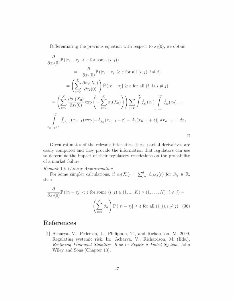
Differentiating the previous equation with respect to xℓ(0), we obtain
∂
∂xℓ(0)P (|τi − τj | < ε for some (i, j))
= −∂
∂xℓ(0)P (|τi − τj| ≥ ε for all (i, j), i 6= j)
=
(
K∑
i=0
∂αi(X0)
∂xℓ(0)
)
P (|τi − τj | ≥ ε for all (i, j), i 6= j)
=
(
K∑
i=0
∂αi(X0)
∂xℓ(0)exp
(
−
K∑
i=0
αi(X0)
))
∑
j∈P
∞
0
fj1(x1)
∞
x1+ε
fj2(x2) . . .
∞
xK−2+ε
fjK−1(xK−1) exp [−AjK (xK−1 + ε)− A0(xK−1 + ε)] dxK−1 . . . dx1
Given estimates of the relevant intensities, these partial derivatives areeasily computed and they provide the information that regulators can useto determine the impact of their regulatory restrictions on the probabilityof a market failure.
Remark 19. (Linear Approximation)For some simpler calculations, if αi(Xr) =
∑d
j=1 βijxj(r) for βij ∈ R,then
∂
∂xℓ(0)P (|τi − τj | < ε for some (i, j) ∈ (1, ..., K)× (1, . . . , K) , i 6= j) =
(
K∑
i=0
βiℓ
)
P (|τi − τj | ≥ ε for all (i, j), i 6= j) (36)
References
[1] Acharya, V., Pedersen, L., Philippon, T., and Richardson, M. 2009.Regulating systemic risk. In: Acharya, V., Richardson, M. (Eds.),Restoring Financial Stability: How to Repair a Failed System. JohnWiley and Sons (Chapter 13).
27
[2] Acemoglu, D., Ozdaglar, A., and Tahbaz-Salehi, A. 2015. Systemic riskand stability in financial networks, American Economic Review, 105(2), 564 - 608.
[3] Allen, F. and Carletti, E. 2013, What is systemic risk?, Journal ofMoney, Credit and Banking, 45(1), 121 - 127.
[4] Berndt, A, Duffie, D., and Zhu, Y. 2021. The Decline of Too Big toFail, working paper, Stanford University.
[5] Bank for International Settlements, Basel Commitee on Banking Super-vision, The G-SIB assessment methodology - score calculation, Novem-ber 2014.
[6] Bisias, D., Flood, M., Lo, A., and Valavanis, S. 2012. A survey ofsystemic risk analytics, Annual Reviw of Financial Economics, 4, 255 -296.
[7] Campbell, J. Y., Hilscher, J., and Szilagyi, J. 2008. In search of distressrisk, Journal of Finance, 63(6), 2899–2939.
[8] Chava, S. and Jarrow, R. 2004. Bankruptcy prediction with industryeffects, Review of Finance, 8(4), 537 - 569.
[9] Crouhy, M., Jarrow, R., and Turnbull, S. 2008. The subprime creditcrisis of 2007, Journal of Derivatives, Fall, 81 - 110.
[10] Engle, R. 2018, Systemic risk 10 years later, Annual Review of FinancialEconomics, 10, 125 - 152.
[11] https://www.fsb.org/2020/11/2020-list-of-global-systemically-important-banks-g-sibs/
[12] Jarrow, R., Lamichhane, S. 2021. Asset price bubbles, market liquidity,and systemic risk. Mathematics and Financial Economics, 15(1), 5 - 40.
[13] Protter, P. 2009. The financial meltdown. SMF-Gazette, 119, 76–82.
[14] Protter, P. and Quintos, A. 2021. Dependent stopping times. workingpaper, Columbia University.
[15] Schich, S. and Toader, O. 2017. To be or not to be a G-SIB: does itmatter?, Journal of Financial Management Markets and Institutions, 5(2), 169 - 192.
28
[16] Shumway, T. 2001. Forecasting bankruptcy more accurately: a simplehazard model, Journal of Business, 74(1), 101–124.
29