Benjamin McKay

Concrete Algebra

With a View Toward Abstract Algebra

September 27, 2018

This work is licensed under a Creative Commons Attribution-ShareAlike 3.0 Unported License.

iii

Preface

With my full philosophical rucksack I can only climb slowly up the moun-tain of mathematics.

— Ludwig WittgensteinCulture and Value

These notes are from lectures given in 2015 at University College Cork. They aimto explain the most concrete and fundamental aspects of algebra, in particular thealgebra of the integers and of polynomial functions of a single variable, groundedby proofs using mathematical induction. It is impossible to learn mathematics byreading a book like you would read a novel; you have to work through exercises andcalculate out examples. You should try all of the problems. More importantly, sincethe purpose of this class is to give you a deeper feeling for elementary mathematics,rather than rushing into advanced mathematics, you should reflect about how thefollowing simple ideas reshape your vision of algebra. Consider how you can useyour new perspective on elementary mathematics to help you some day guide otherstudents, especially children, with surer footing than the teachers who guided you.

v

vi

The temperature of Heaven can be rather accurately computed.Our authority is Isaiah 30:26, “Moreover, the light of the Moonshall be as the light of the Sun and the light of the Sun shallbe sevenfold, as the light of seven days.” Thus Heaven receivesfrom the Moon as much radiation as we do from the Sun, and inaddition 7 × 7 = 49 times as much as the Earth does from theSun, or 50 times in all. The light we receive from the Moon isone 1/10 000 of the light we receive from the Sun, so we can ignorethat. . . . The radiation falling on Heaven will heat it to the pointwhere the heat lost by radiation is just equal to the heat received byradiation, i.e., Heaven loses 50 times as much heat as the Earth byradiation. Using the Stefan-Boltzmann law for radiation, (H/E)temperature of the earth (∼ 300 K), gives H as 798 K (525 ◦C).The exact temperature of Hell cannot be computed. . . . [However]Revelations 21:8 says “But the fearful, and unbelieving . . . shallhave their part in the lake which burneth with fire and brimstone.”A lake of molten brimstone means that its temperature must be ator below the boiling point, 444.6 ◦C. We have, then, that Heaven,at 525 ◦C is hotter than Hell at 445 ◦C.

— Applied Optics , vol. 11, A14, 1972

In these days the angel of topology and the devil of abstract algebrafight for the soul of every individual discipline of mathematics.

— Hermann WeylInvariants, Duke Mathematical Journal 5, 1939, 489–502

— and so who are you, after all?— I am part of the power which forever wills evil and forever worksgood.

— GoetheFaust

This Book is not to be doubted.— Quran , 2:1/2:6-2:10 The Cow

Contents

1 The integers 12 Mathematical induction 93 Greatest common divisors 174 Prime numbers 235 Modular arithmetic 276 Secret messages 417 Rational, real and complex numbers 458 Polynomials 519 Real polynomials, complex polynomials 5910 Factoring polynomials 6911 Resultants and discriminants 7712 Groups 8913 Permuting roots 11314 Fields 12515 Field extensions 13116 Rings 13717 Galois theory 14318 Algebraic curves in the plane 14719 Where plane curves intersect 15720 Quotient rings 16321 Field extensions and algebraic curves 17122 The projective plane 17523 Algebraic curves in the projective plane 18124 Families of plane curves 19525 Elliptic curves 20526 The tangent line 20927 Inflection points 21928 Conics and quadratic forms 22729 Projective duality 23330 Polynomial equations have solutions 23531 More projective planes 239

vii

viii Contents

Hints 259Bibliography 277List of notation 279Index 281

Chapter 1

The integers

God made the integers; all else is the work of man.

— Leopold Kronecker

Notation

We will write numbers using notation like 1 234 567.123 45, using a decimal point . atthe last integer digit, and using thin spaces to separate out every 3 digits before orafter the decimal point. You might prefer 1,234,567·123,45 or 1,234,567.123,45, whichare also fine. We reserve the · symbol for multiplication, writing 2 · 3 = 6 rather than2× 3 = 6.

The laws of integer arithmetic

The integers are the numbers . . . ,−2,−1, 0, 1, 2, . . .. Let us distill their essentialproperties, using only the concepts of addition and multiplication.

Addition laws:

a. The associative law: For any integers a, b, c: (a+ b) + c = a+ (b+ c).b. The identity law: There is an integer 0 so that for any integer a: a+ 0 = a.c. The existence of negatives: for any integer a: there is an integer b (denoted

by the symbol −a) so that a+ b = 0.d. The commutative law: For any integers a, b: a+ b = b+ a.

Multiplication laws:

a. The associative law: For any integers a, b, c: (ab)c = a(bc).b. The identity law: There is an integer 1 so that for any integer a: a1 = a.c. The zero divisors law: For any integers a, b: if ab = 0 then a = 0 or b = 0.d. The commutative law: For any integers a, b: ab = ba.

The distributive law:

a. For any integers a, b, c: a(b+ c) = ab+ ac.

1

2 The integers

Sign laws:Certain integers are called positive.

a. The succession law: An integer b is positive just when either b = 1 orb = c+ 1 for a positive integer c.

b. Determinacy of sign: Every integer a has precisely one of the followingproperties: a is positive, a = 0, or −a is positive.

We write a < b to mean that there is a positive integer c so that b = a+ c.

The law of well ordering:

a. Any nonempty collection of positive integers has a least element; that isto say, an element a so that every element b satisfies a < b or a = b.

All of the other arithmetic laws we are familiar with can be derived from these. Forexample, the associative law for addition, applied twice, shows that (a+ b) + (c+d) =a+ (b+ (c+ d)), and so on, so that we can add up any finite sequence of integers, inany order, and get the same result, which we write in this case as a + b + c + d. Asimilar story holds for multiplication.

Of course, we write 1 + 1 as 2, and 1 + 1 + 1 as 3 and so on. Write a > b to meanb < a. Write a ≤ b to mean a < b or a = b. Write a ≥ b to mean b ≤ a. Write |a| tomean a, if a ≥ 0, and to mean −a otherwise, and call it the absolute value of a. Aninteger a is negative if −a is positive.

To understand mathematics, you have to solve a large number of problems.

I prayed for twenty years but received no answer until I prayed with mylegs.

— Frederick Douglass, statesman and escaped slave

1.1 For each equation below, what law above justifies it?

a. 7(3 + 1) = 7 · 3 + 7 · 1b. 4(9 · 2) = (4 · 9)2c. 2 · 3 = 3 · 2

1.2 Use the laws above to prove that for any integers a, b, c: (a+ b)c = ac+ bc.

1.3 Use the laws above to prove that 0 + 0 = 0.

1.4 Use the laws above to prove that 0 · 0 = 0.

1.5 Use the laws above to prove that, for any integer a: a · 0 = 0.

The laws of integer arithmetic 3

1.6 Use the laws above to prove that, for any integer a: there is exactly one integerb so that a+ b = 0; of course, we call this b by the name −a.

1.7 Use the laws above to prove that, for any integer a: (−1)a = −a.

1.8 Use the laws above to prove that (−1)(−1) = 1.

1.9 Use the laws above to prove that, for any integers b, c: |bc| = |b||c|.

1.10 Our laws ensure that there is an integer 0 so that a + 0 = 0 + a = a for anyinteger a. Could there be two different integers, say p and q, so that a+p = p+a = afor any integer a, and also so that a + q = q + a = a for any integer a? (Roughlyspeaking, we are asking if there is more than one integer which can “play the role” ofzero.)

1.11 Our laws ensure that there is an integer 1 so that a · 1 = 1 ·a = a for any integera. Could there be two different integers, say p and q, so that ap = pa = a for anyinteger a, and also so that aq = qa = a for any integer a?

Theorem 1.1 (The equality cancellation law for addition). Suppose that a, b and care integers and that a+ c = b+ c. Then a = b.

Proof. By the existence of negatives, there is a integer −c so that c + (−c) = 0.Clearly (a + c) + (−c) = (b + c) + (−c). Apply the associative law for addition:a+ (c+ (−c)) = b+ (c+ (−c)), so a+ 0 = b+ 0, so a = b.

1.12 Prove that −(b+ c) = (−b) + (−c) for any integers b, c.

We haven’t mentioned subtraction yet.

1.13 Suppose that a and b are integers. Prove that there is a unique integer c so thata = b+ c. Of course, from now on we write this integer c as a− b.

1.14 Prove that, for any integers a, b, a− b = a+ (−b).

1.15 Prove that subtraction distributes over multiplication: for any integers a, b, c,a(b− c) = ab− ac.

1.16 Prove that any two integers b and c satisfy just precisely one of the conditionsb > c, b = c, b < c.

Theorem 1.2. The equality cancellation law for multiplication: for an integers a, b, cif ab = ac and a 6= 0 then b = c.

Proof. If ab = ac then ab−ac = ac−ac = 0. But ab−ac = a(b−c) by the distributivelaw. So a(b− c) = 0. By the zero divisors law, a = 0 or b = c.

1.17 We know how to add and multiply 2× 2 matrices with integer entries. Of thevarious laws of addition and multiplication and signs for integers, which hold true alsofor such matrices?

1.18 Use the laws above to prove that the sum of any two positive integers is positive.

1.19 Use the laws above to prove that the product of any two positive integers ispositive.

4 The integers

1.20 Use the laws above to prove that the product of any two integers is positive justwhen (1) both are positive or (2) both are negative.

1.21 Use the laws above to prove that the product of any two negative integers ispositive.

1.22 Prove the inequality cancellation law for addition: For any integers a, b, c: ifa+ c < b+ c then a < b.

1.23 Prove the inequality cancellation law for multiplication: For any integers a, b, c:if a < b and if 0 < c then ac < bc.

Division of integers

Can you do Division? Divide a loaf by a knife—what’s the answer tothat?

— Lewis CarrollThrough the Looking Glass

We haven’t mentioned division yet. Danger: although 2 and 3 are integers,

32 = 1.5

is not an integer.

1.24 Suppose that a and b are integers and that b 6= 0. Prove from the laws abovethat there is at most one integer c so that a = bc. Of course, from now on we writethis integer c as a

bor a/b.

1.25 Danger: why can’t we divide by zero?

We already noted that 3/2 is not an integer. At the moment, we are trying towork with integers only. An integer b divides an integer c if c/b is an integer; we alsosay that b is a divisor of c.

1.26 Explain why every integer divides into zero.

1.27 Prove that, for any two integers b and c, the following are equivalent:

a. b divides c,

b. −b divides c,

c. b divides −c,

d. −b divides −c,

e. |b| divides |c|.

Proposition 1.3. Take any two integers b and c. If b divides c, then |b| < |c|or b = c or b = −c.

Division of integers 5

Proof. By the solution of the last problem, we can assume that b and c are positive. Ifb = c the proposition holds, so suppose that b > c; write b = c+k for some k > 0. Sinceb divides c, say c = qb for some integer q. Since b > 0 and c > 0, q > 0 by problem 1.20on the facing page. If q = 1 then c = b, so the proposition holds. If q > 1, thenq = n+1 for some positive integer n. But then c = qb = (n+1)(c+k) = nc+c+nk+k.Subtract c from both sides: 0 = nc+nk+k, a sum of positive integers, hence positive(by problem 1.19 on page 3) a contradiction.

1.28 Suppose that S is a set of integers. A lower bound on S is an integer b so thatb ≤ c for every integer c from S; if there is a lower bounded, S is bounded from below.Prove that a nonempty set of integers bounded from below contains a least element.

Theorem 1.4 (Euclid). Suppose that b and c are integers and c 6= 0. Then thereare unique integers q and r (the quotient and remainder) so that b = qc+ r and sothat 0 ≤ r < |c|.

Proof. To make our notation a little easier, we can assume (by perhaps changing thesigns of c and q in our statement above) that c > 0.

Consider all integers of the form b− qc, for various integers q. If we were to takeq = −|b|, then b− qc = b+ |b|+ (c− 1)|b| ≥ 0. By the law of well ordering, since thereis an integer of the form b− qc ≥ 0, there is a smallest integer of the form b− qc ≥ 0;call it r. If r ≥ c, we can replace r = b− qc by r − c = b− (q + 1)c, and so r was notsmallest.

We have proven that we can find a quotient q and remainder r. We need to showthat they are unique. Suppose that there is some other choice of integers Q and Rso that b = Qc + R and 0 ≤ R < c. Taking the difference between b = qc + r andb = Qc + R, we find 0 = (Q − q)c + (R − r). In particular, c divides into R − r.Switching the labels as to which ones are q, r and which are Q,R, we can assume thatR ≥ r. So then 0 ≤ r ≤ R < c, so R− r < c. By proposition 1.3 on the facing page,since 0 ≤ R− r < c and c divides into R− r, we must have R− r = 0, so r = R. Pluginto 0 = (Q− q)c+ (R− r) to see that Q = q.

How do we actually find quotient and remainder, by hand? Long division:

1417)

249170796811

So if we start with b = 249 and c = 17, we carry out long division to find the quotientq = 14 and the remainder r = 11.

1.29 Find the quotient and remainder for b, c equal to:a. −180, 9b. −169, 11c. −982,−11d. 279,−11e. 247,−27

6 The integers

The greatest common divisor

A common divisor of some integers is an integer which divides them all.

1.30 Given any collection of one or more integers, not all zero, prove that they havea greatest common divisor , i.e. a largest positive integer divisor.

Denote the greatest common divisor of integers m1,m2, . . . ,mn as

gcd {m1,m2, . . . ,mn} .

If the greatest common divisor of two integers is 1, they are coprime. We will alsodefine gcd {0, 0, . . . , 0} ..= 0.

Lemma 1.5. Take two integers b, c with c 6= 0 and compute the quotient q andremainder r, so that b = qc+ r and 0 ≤ r < |c|. Then the greatest common divisorof b and c is the greatest common divisor of c and r.

Proof. Any divisor of c and r divides the right hand of the equation b = qc+ r, so itdivides the left hand side, and so divides b and c. By the same reasoning, writing thesame equation as r = b− qc, we see that any divisor of b and c divides c and r.

This makes very fast work of finding the greatest common divisor by hand. For exam-ple, if b = 249 and c = 17 then we found that q = 14 and r = 11, so gcd {249, 17} =gcd {17, 11}. Repeat the process: taking 17 and dividing out 11, the quotient andremainder are 1, 6, so gcd {17, 11} = gcd {11, 6}. Again repeat the process: the quo-tient and remainder for 11, 6 are 1, 5, so gcd {11, 6} = gcd {6, 5}. Again repeat theprocess: the quotient and remainder for 11, 6 are 1, 5, so gcd {11, 6} = gcd {6, 5}. Inmore detail, we divide the smaller integer (smaller in absolute value) into that thelarger:

1417)

249170796811

Throw out the larger integer, 249, and replace it by the remainder, 11, and divideagain:

111)

17116

Again we throw out the larger integer (in absolute value), 17, and replace with theremainder, 6, and repeat:

16)

1165

The least common multiple 7

and again:1

5)

651

and again:5

1)

550

The remainder is now zero. The greatest common divisor is therefore 1, the finalnonzero remainder: gcd {249, 17} = 1.

This method to find the greatest common divisor is called the Euclidean algorithm.

If the final nonzero integer is negative, just change its sign to get the greatest commondivisor.

gcd {−4,−2} = gcd {−2, 0} = gcd {−2} = 2.

1.31 Find the greatest common divisor ofa. 4233, 884b. -191, 78c. 253, 29d. 84, 276e. -92, 876f. 147, 637g. 266 664, 877 769

The least common multiple

The least common multiple of a finite collection of integersm1,m2, . . . ,mn is the small-est positive integer ` = lcm {m1,m2, . . . ,mn} so that all of the integersm1,m2, . . . ,mn

divide `.

Lemma 1.6. The least common multiple of any two integers b, c (not both zero) is

lcm {b, c} = |bc|gcd {b, c} .

Proof. For simplicity, assume that b > 0 and c > 0; the cases of b ≤ 0 or c ≤ 0 aretreated easily by flipping signs as needed and checking what happens when b = 0or when c = 0 directly; we leave this to the reader. Let d ..= gcd {b, c}, and factorb = Bd and c = Cd. Then B and C are coprime. Write the least common multiple` of b, c as either ` = b1b or as ` = c1c, since it is a multiple of both b and c. Sothen ` = b1Bd = c1Cd. Cancelling, b1B = c1C. So C divides b1B, but doesn’tdivide B, so divides b1, say b1 = b2C, so ` = b1Bd = b2CBd. So BCd divides `. So(bc)/d = BCd divides `, and is a multiple of b: BCd = (Bd)C = bC, and is a multipleof c: BCd = B(Cd) = Bc. But ` is the least such multiple.

8 The integers

Sage

Computers are useless. They can only give you answers.

— Pablo Picasso

These lecture notes include optional sections explaining the use of the sage computeralgebra system. At the time these notes were written, instructions to install sageon a computer are at www.sagemath.org, but you should be able to try out sage onsagecell.sagemath.org or even create worksheets in sage on cocalc.com over theinternet without installing anything on your computer. If we type

gcd(1200,1040)

and press shift–enter, we see the greatest common divisor: 80. Similarly type

lcm(1200,1040)

and press shift–enter, we see the least common multiple: 15600. Sage can carry outcomplicated arithmetic operations. The multiplication symbol is *:

12345*13579

gives 167632755. Sage uses the expression 2^3 to mean 23. You can invent variablesin sage by just typing in names for them. For example, ending each line with enter,except the last which you end with shift–enter (when you want sage to computeresults):

x=4y=7x*y

to print 28. The expression 15 % 4 means the remainder of 15 divided by 4, while15//4 means the quotient of 15 divided by 4. We can calculate the greatest commondivisor of several integers as

gcd([3800,7600,1900])

giving us 1900.

Chapter 2

Mathematical induction

It is sometimes required to prove a theorem which shall be truewhenever a certain quantity n which it involves shall be an integeror whole number and the method of proof is usually of the followingkind. 1st. The theorem is proved to be true when n = 1. 2ndly.It is proved that if the theorem is true when n is a given wholenumber, it will be true if n is the next greater integer. Hence thetheorem is true universally.

— George Boole

So nat’ralists observe, a fleaHas smaller fleas that on him prey;And these have smaller fleas to bite ’em.And so proceeds Ad infinitum.

— Jonathan SwiftOn Poetry: A Rhapsody

It is often believed that everyone with red hair must have a red haired ancestor. Butthis principle is not true. We have all seen someone with red hair. According to theprinciple, she must have a red haired ancestor. But then by the same principle, hemust have a red haired ancestor too, and so on. So the principle predicts an infinitechain of red haired ancestors. But there have only been a finite number of creatures(so the geologists tell us). So some red haired creature had no red haired ancestor.

We will see that1 + 2 + 3 + · · ·+ n = n(n+ 1)

2for any positive integer n. First, let’s check that this is correct for a few values ofn just to be careful. Danger: just to be very careful, we put ?= between any twoquantities when we are checking to see if they are equal; we are making clear thatwe don’t yet know.

For n = 1, we get 1 ?= 1(1 + 1)/2, which is true because the right hand side is1(1 + 1)/2) = 2/2 = 1.

For n = 2, we need to check 1+2 ?= 2(2+1)/2. The left hand side of the equationis 3, while the right hand side is:

2(2 + 1)2 = 2(3)

2 = 3,

9

10 Mathematical induction

So we checked that they are equal.For n = 3, we need to check that 1 + 2 + 3 ?= 3(3 + 1)/2. The left hand side is

6, and you can check that the right hand side is 3(4)/2 = 6 too. So we checked thatthey are equal.

But this process will just go on for ever and we will never finish checking all valuesof n. We want to check all values of n, all at once.

Picture a row of dominoes. If we can make the first domino topple, and we canmake sure that each domino, if it topples, will make the next domino topple, thenthey will all topple.

Theorem 2.1 (The Principle of Mathematical Induction). Take a collection of pos-itive integers. Suppose that 1 belongs to this collection. Suppose that, whenever allpositive integers less than a given positive integer n belong to the collection, then sodoes the integer n. (For example, if 1, 2, 3, 4, 5 belong, then so does 6, and so on.)Then the collection consists precisely of all of the positive integers.

Proof. Let S be the set of positive integers not belonging to that collection. If S isempty, then our collection contains all positive integers, so our theorem is correct.But what is S is not empty? By the law of well ordering, if S is not empty, then Shas a least element, say n. So n is not in our collection. But being the least integernot in our collection, all integers 1, 2, . . . , n− 1 less than n are in our collection. Byhypothesis, n is also in our collection, a contradiction to our assumption that S is notempty.

Let’s prove that 1+2+3+ · · ·+n = n(n+1)/2 for any positive integer n. First, notethat we have already checked this for n = 1 above. Imagine that we have checkedour equation 1 + 2 + 3 + · · ·+ n = n(n+ 1)/2 for any positive integer n up to, butnot including, some integer n = k. Now we want to check for n = k whether it is stilltrue: 1 + 2 + 3 + · · ·+ n

?= n(n+ 1)/2. Since we already know this for n = k− 1, weare allowed to write that out, without question marks:

1 + 2 + 3 + · · ·+ k − 1 = (k − 1)(k − 1 + 1)/2.

Simplify:1 + 2 + 3 + · · ·+ k − 1 = (k − 1)k/2.

Now add k to both sides. The left hand side becomes 1 + 2 + 3 + · · ·+ k. The righthand side becomes (k − 1)k/2 + k, which we simplify to

(k − 1)k2 + k = (k − 1)k

2 + 2k2 ,

= k2 − k + 2k2 ,

= k2 + k

2 ,

= k(k + 1)2 .

So we have found that, as we wanted to prove,

1 + 2 + 3 + · · ·+ k = k(k + 1)2 .

Mathematical induction 11

Note that we used mathematical induction to prove this: we prove the result forn = 1, and then suppose that we have proven it already for all values of n up to somegiven value, and then show that this will ensure it is still true for the next value.

The general pattern of induction arguments: we start with a statement we wantto prove, which contains a variable, say n, representing a positive integer.

a. The base case: Prove your statement directly for n = 1.b. The induction hypothesis: Assume that the statement is true for all positive

integer values less than some value n.c. The induction step: Prove that it is therefore also true for that value of n.

We can use induction in definitions, not just in proofs. We haven’t made sense yetof exponents. (Exponents are often called indices in Irish secondary schools, butnowhere else in the world to my knowledge).

a. The base case: For any integer a 6= 0 we define a0 ..= 1. Watch: We can write..= instead of = to mean that this is our definition of what a0 means, not anequation we have somehow calculated out. For any integer a (including thepossibility of a = 0) we also define a1 ..= a.

b. The induction hypothesis: Suppose that we have defined already what

a1, a2, . . . , ab

means, for some positive integer b.c. The induction step: We then define ab+1 to mean ab+1 ..= a · ab.For example, by writing out

a4 = a · a3,

= a · a · a2,

= a · a · a · a1,

= a · a · a · a︸ ︷︷ ︸4 times

.

Another example:a3a2 = (a · a · a) (a · a) = a5.

In an expression ab, the quantity a is the mantissa or base and b is the exponent.

2.1 Use induction to prove that ab+c = abac for any integer a and for any positiveintegers b, c.

2.2 Use induction to prove that(ab)c = abc for any integer a and for any positive

integers b, c.

Sometimes we start induction at a value of n which is not at n = 1.Let’s prove, for any integer n ≥ 2, that 2n+1 < 3n.

a. The base case: First, we check that this is true for n = 2: 22+1 < 32? Simplifyto see that this is 8 < 9, which is clearly true.

b. The induction hypothesis: Next, suppose that we know this is true for all valuesn = 2, 3, 4, . . . , k − 1.

12 Mathematical induction

c. The induction step: We need to check it for n = k: 2k+1 < 3k? How can werelate this to the values n = 2, 3, 4, . . . , k − 1?

2k+1 = 2 · 2k,

< 3 · 3k−1 by assumption,

= 3k.

We conclude that 2n+1 < 3n for all integers n ≥ 2.

2.3 All horses are the same colour; we can prove this by induction on the number ofhorses in a given set.

a. The base case: If there’s just one horse then it’s the same colour as itself, sothe base case is trivial.

b. The induction hypothesis: Suppose that we have proven that, in any set of atmost k horses, all of the horses are the same colour as one another, for anynumber k = 1, 2, . . . , n.

c. The induction step: Assume that there are n horses numbered 1 to n. By theinduction hypothesis, horses 1 through n− 1 are the same color as one another.Similarly, horses 2 through n are the same color. But the middle horses, 2through n − 1, can’t change color when they’re in different groups; these arehorses, not chameleons. So horses 1 and n must be the same color as well.

Thus all n horses are the same color. What is wrong with this reasoning?

2.4 We could have assumed much less about the integers than the laws we gave inchapter 1. Using only the laws for addition and induction,

a. Explain how to define multiplication of integers.b. Use your definition of multiplication to prove the associative law for multiplica-

tion.c. Use your definition of multiplication to prove the equality cancellation law for

multiplication.

2.5 Suppose that x, b are positive integers. Prove that x can be written as

x = a0 + a1b+ a2b2 + · · ·+ akb

k

for unique integers a0, a1, . . . , ak with 0 ≤ ai < b. Hint: take quotient and remainder,and apply induction. (The sequence ak, ak−1, . . . , a1, a0 is the sequence of digits of xin base b notation.)

2.6 Prove that for every positive integer n,

13 + 23 + · · ·+ n3 =(n(n+ 1)

2

)2

.

2.7 Picture a 2× 2 grid, a 4× 4 grid, an 8× 8 grid, a 16× 16 grid, and so on.

. . .

Sage 13

Fix a positive integer n. Show that it is possible to tile any 2n × 2n grid, but withexactly one square removed, using ’L’-shaped tiles of three squares: .

Sage

A computer once beat me at chess, but it was no match for me at kickboxing.

— Emo Philips

To define a function in sage, you type def, to mean define, like:

def f(n):return 2*n+1

and press shift–enter. For any input n, it will return a value f(n) = 2n+ 1. Carefulabout the * for multiplication. Use your function, for example, by typing

f(3)

and press shift–enter to get 7.A function can depend on several inputs:

def g(x,y):return x*y+2

A recursive function is one whose value for some input depends on its value forother inputs. For example, the sum of the integers from 1 to n is:

def sum_of_integers(n):if n<=0:

return 0else:

return n+sum_of_integers(n-1)

giving us sum_of_integers(5) = 15.

2.8 The Fibonnaci sequence is F (1) = 1, F (2) = 1, and F (n) = F (n− 1) + F (n− 2)for n ≥ 3. Write out a function F(n) in sage to compute the Fibonacci sequence.

Lets check that 2n+1 < 3n for some values of n, using a loop:

for n in [0..10]:print(n,3^n-2^(n+1))

This will try successively plugging in each value of n starting at n = 0 and going upto n = 1, n = 2, and so on up to n = 10, and print out the value of n and the valueof 3n − 2n+1. It prints out:

14 Mathematical induction

(0, -1)(1, -1)(2, 1)(3, 11)(4, 49)(5, 179)(6, 601)(7, 1931)(8, 6049)(9, 18659)(10, 57001)

giving the value of n and the value of the difference 3n − 2n+1, which we can readilysee is positive once n ≥ 2. Tricks like this help us to check our induction proofs.

If we write a=a+1 in sage, this means that the new value of the variable a is equalto one more than the old value that a had previously. Unlike mathematical variables,sage variables can change value over time. In sage the expression a<>b means a 6= b.Although sage knows how to calculate the greatest common divisor of some integers,we can define own greatest common divisor function:

def my_gcd(a, b):while b<>0:

a,b=b,a%breturn a

We could also write a greatest divisor function that uses repeated subtraction, avoidingthe quotient operation %:

def gcd_by_subtraction(a, b):if a<0:

a=-aif b<0:

b=-bif a==0:

return bif b==0:

return awhile a<>b:

if a>b:a=a-b

else:b=b-a

return a

Lists in sage

Sage manipulates lists. A list is a finite sequence of objects written down next to oneanother. The list L=[4,4,7,9] is a list called L which consists of four numbers: 4, 4, 7and 9, in that order. Note that the same entry can appear any number of times; inthis example, the number 4 appears twice. You can think of a list as like a vector in

Lists in sage 15

Rn, a list of numbers. When you “add” lists they concatenate: [6]+[2] yields [6, 2].Sage uses notation L[0], L[1], and so on, to retrieve the elements of a list, instead ofthe usual vector notation. Warning: the element L[1] is not the first element. Thelength of a list L is len(L). To create a list [0, 1, 2, 3, 4, 5] of successive integer, typerange(0,6). Note that the number 6 here tells you to go up to, but not include, 6.So a L list of 6 elements has elements L0, L1, . . . , L5, denoted L[0], L[1], . . . , L[5] insage. To retrieve the list of elements of L from L2 to L4, type L[2:5]; again strangelythis means up to but not including L5.

For example, to reverse the elements of a list:

def reverse(L):n=len(L)if n<=1:

return Lelse:

return L[n-1:n]+reverse(L[0:n-1])

We create a list with 10 entries, print it:

L=range(0,10)print(L)

yielding [0, 1, 2, 3, 4, 5, 6, 7, 8, 9] and then print its reversal:

print(reverse(L))

yielding [9, 8, 7, 6, 5, 4, 3, 2, 1, 0].We can construct a list of elements of the Fibonacci sequence:

def fibonacci_list(n):L=[1,1]for i in range(2,n):

L=L+[L[i-1]+L[i-2]]return L

so that fibonacci_list(10) yields [1, 1, 2, 3, 5, 8, 13, 21, 34, 55], a list of the first tennumbers in the Fibonacci sequence. The code works by first creating a list L=[1,1]with the first two entries in it, and then successively building up the list L by con-catenating to it a list with one more element, the sum of the two previous list entries,for all values i = 2, 3, . . . , n.

Chapter 3

Greatest common divisors

The laws of nature are but the mathematical thoughts of God.

— Euclid

Euclid alone has looked on Beauty bare.Let all who prate of Beauty hold their peace,And lay them prone upon the earth and ceaseTo ponder on themselves, the while they stareAt nothing, intricately drawn nowhereIn shapes of shifting lineage; let geeseGabble and hiss, but heroes seek releaseFrom dusty bondage into luminous air.O blinding hour, O holy, terrible day,When first the shaft into his vision shoneOf light anatomized! Euclid aloneHas looked on Beauty bare. Fortunate theyWho, though once only and then but far away,Have heard her massive sandal set on stone.

— Edna St. Vincent MillayEuclid Alone

The extended Euclidean algorithm

Theorem 3.1 (Bézout). For any two integers b, c, not both zero, there are integers s, tso that sb+ tc = gcd {b, c}.

These Bézout coefficients s, t play an essential role in advanced arithmetic, as wewill see.To find the Bézout coefficients of 12, 8, write out a matrix(

1 0 120 1 8

).

Repeatedly add some integer multiple of one row to the other, to try to make thebigger number in the last column (bigger by absolute value) get smaller (by absolutevalue). In this case, we can subtract row 2 from row 1, to get rid of as much of the

17

18 Greatest common divisors

12 as possible. All operations are carried out a whole row at a time:(1 −1 40 1 8

)Now the bigger number (by absolute value) in the last column is the 8. We subtractas large an integer multiple of row 1 from row 2, in this case subtract 2 (row 1) fromrow 2, to kill as much of the 8 as possible:(

1 −1 4−2 3 0

)Once we get a zero in the last column, the other entry in the last column is thegreatest common divisor, and the entries in the same row as the greatest commondivisor are the Bézout coefficients. In our example, the Bézout coefficients of 12, 8 are1,−1 and the greatest common divisor is 4. This trick to calculate Bézout coefficientsis the extended Euclidean algorithm.

Again, we have to be a little bit careful about minus signs. For example, if we lookat −8,−4, we find Bézout coeffiicients by(

1 0 −80 1 −4

)→(

1 −2 00 1 −4

),

the process stops here, and where we expect to get an equation sb+ tc = gcd {b, c},instead we get

0(−8) + 1(−4) = −4,which has the wrong sign, a negative greatest common divisor. So if the answerpops out a negative for the greatest common divisor, we change signs: t = 0, s =−1, gcd {b, c} = 4.

Theorem 3.2. The extended Euclidean algorithm calculates Bézout coefficients. Inparticular, Bézout coefficients s, t exist for any integers b, c with c 6= 0.

Proof. At each step in the extended Euclidean algorithm, the third column proceedsexactly by the Euclidean algorithm, replacing the larger number (in absolute value)with the remainder by the division, except for perhaps a minus sign. So at the laststep, the last nonzero number in the third column is the greatest common divisor,except for perhaps a minus sign.

Our extended Euclidean algorithm starts with(1 0 b0 1 c

),

a matrix which satisfies (1 0 b0 1 c

)( bc−1

)=(

00

),

It is easy to check that if some 2× 3 matrix M satisfies

M

(bc−1

)=(

00

),

The greatest common divisor of several numbers 19

then so does the matrix you get by adding any multiple of one row of M to the otherrow.

Eventually we get a zero in the final column, say(s t dS T 0

),

or (s t 0S T D

).

It doesn’t matter which since, at any step, we could always swap the two rows withoutchanging the steps otherwise. So suppose we end up at(

s t dS T 0

).

But (s t dS T 0

)( bc−1

)=(sb+ tc− d

0

).

This has to be zero, so: sb+ tc = d.

Proposition 3.3. Take two integers b, c, not both zero. The number gcd {b, c} isprecisely the smallest positive integer which can be written as sb+ tc for some integerss, t.

Proof. Let d ..= gcd {b, c}. Since d divides into b, we divide it, say as b = Bd, for someinteger B. Similarly, b = Cd for some integer C. Imagine that we write down somepositive integer as sb+tc for some integers s, t. Then sb+sc = sBd+tCd = (sB+tC)dis a multiple of d, so no smaller than d.

3.1 Find Bézout coefficients and greatest common divisors ofa. 2468, 180b. 79, -22c. 45,16d. -1000,2002

The greatest common divisor of several numbers

Take several integers, say m1,m2, . . . ,mn, not all zero. To find their greatest commondivisor, we only have to find the greatest common divisor of the greatest commondivisors. For example,

gcd {m1,m2,m3} = gcd {gcd {m1,m2} ,m3}

andgcd {m1,m2,m3,m4} = gcd {gcd {m1,m2} , gcd {m3,m4}}

and so on.

3.2 Use this approach to find gcd {54, 90, 75}.

20 Greatest common divisors

Bézout coefficients of several numbers

Take integers m1,m2, . . . ,mn, not all zero. We will see that their greatest commondivisor is the smallest positive integer d so that

d = s1m1 + s2m2 + · · ·+ snmn

for some integers s1, s2, . . . , sn, the Bézout coefficients of m1,m2, . . . ,mn. To find theBézout coefficients, and the greatest common divisor:

a. Write down the matrix: 1 0 0 . . . 0 m10 1 0 . . . 0 m20 0 1 . . . 0 m3...

......

.... . .

...0 0 0 . . . 1 mn

b. Subtract whatever integer multiples of rows from other rows, repeatedly, until

the final column has exactly one nonzero entry.c. That nonzero entry is the greatest common divisor

d = gcd {m1,m2, . . . ,mn} .

d. The entries in the same row, in earlier columns, are the Bézout coefficients, sothe row looks like (

s1 s2 . . . sn d)

To find Bézout coefficients of 12, 20, 18:(1 0 0 120 1 0 200 0 1 18

)

the smallest entry (in absolute value) in the final column is the 12, so we divide itinto the other two entries:

a. add −row 1 to row 2, andb. −row 1 to row 3: ( 1 0 0 12

−1 1 0 8−1 0 1 6

)Now the smallest (in absolute value) is the 6, so we add integer multiples of its rowto the two earlier rows:

a. add −2 · row 3 to row 1, andb. −row 3 to row 2: ( 3 0 −2 0

0 1 −1 2−1 0 1 6

)Now the 2 is the smallest nonzero entry (in absolute value) in the final column. Note:once a row in the final column has a zero in it, it becomes irrelevant, so we could

Sage 21

save time by crossing it out and deleting it. That happens here with the first row.But we will leave it as it is, just to make the steps easier to follow. Add −3 · row 2to row 3: ( 3 0 −2 0

0 1 −1 2−1 −3 4 0

)Just to carefully check that we haven’t made any mistake, you can compute out thatthis matrix satisfies: ( 3 0 −2 0

0 1 −1 2−1 −3 4 0

)122018−1

=

(000

).

In particular, our Bézout coefficients are the 0, 1,−1, in front of the greatest commondivisor, 2. Summing up:

0 · 12 + 1 · 20 + (−1) · 18 = 2.

3.3 Use this approach to find Bézout coefficients of 54, 90, 75.

3.4 Prove that this method works.

3.5 Explain how to find the least common multiple of three integers a, b, c.

Sage

Computer science is no more about computers than astronomy is abouttelescopes.

— Edsger Dijkstra

The extended Euclidean algorithm is built in to sage: xgcd(12,8) returns (4, 1,−1),the greatest common divisor and the Bézout coefficients, so that 4 = 1 · 12 + (−1) · 8.We can write our own function to compute Bézout coefficients:

def bez(b,c):p,q,r=1,0,bs,t,u=0,1,cwhile u<>0:

if abs(r)>abs(u):p,q,r,s,t,u=s,t,u,p,q,r

Q=u//rs,t,u=s-Q*p,t-Q*q,u-Q*r

return r,p,q

so that bez(45,210) returns a triple (g, s, t) where g is the greatest commmon divisorof 45, 210, while s, t are the Bézout coefficients.

Let’s find Bézout coefficients of several numbers. First we take a matrix A of sizen× (n+ 1). Just as sage has lists L indexed starting at L[0], so sage indexes matrices

22 Greatest common divisors

as Aij for i and j starting at zero, i.e. the upper left corner entry of any matrix A isA[0,0] in sage. We search for a row which has a nonzero entry in the final column:

def row_with_nonzero_entry_in_final_column(A,rows,columns,starting_from_row=0):for i in range(starting_from_row,rows):

if A[i,columns-1]<>0:return i

return rows

Note that we write starting_from_row=0 to give a default value: we can specify a rowto start looking from, but if you call the function rwo_with_nonzero_entry_in_final_columnwithout specifying a value for the variable starting_from_row, then that variablewill take the value 0. We use this to find the Bézout coefficients of a list of integers:

def bez(L):n=len(L)A=matrix(n,n+1)for i in range(0,n):

for j in range(0,n):if i==j:

A[i,j]=1else:

A[i,j]=0A[i,n]=L[i]

k=row_with_nonzero_entry_in_final_column(A,n,n+1)l=row_with_nonzero_entry_in_final_column(A,n,n+1,k+1)while l<n:

if abs(A[l,n])>abs(A[k,n]):k,l=l,k

q=A[k,n]//A[l,n]for j in range(0,n+1):

A[k,j]=A[k,j]-q*A[l,j]k=row_with_nonzero_entry_in_final_column(A,n,n+1)l=row_with_nonzero_entry_in_final_column(A,n,n+1,k+1)

return ([A[k,j] for j in range(0,n)],A[k,n])

Given a list L of integers, we let n be the length of the list L, form a matrix A of sizen × (n + 1), put the identity matrix into its first n columns, and put the entries ofL into its final column. Then we find the first row k with a nonzero entry in the lastcolumn. Then we find the next row l with a nonzero entry in the last column. Swapk and l if needed to get row l to have smaller entry in the last column. Find thequotient q of those entries, dropping remainder. Subtract off q times row l from rowk. Repeat until there is no such row l left. Return a list of the numbers. Test it out:bez([-2*3*5,2*3*7,2*3*11]) yields ([3, 2, 0] ,−6), giving the Bézout coefficients asthe list [3, 2, 0] and the greatest common divisor next: −6.

Chapter 4

Prime numbers

I think prime numbers are like life. They are very logical but you couldnever work out the rules, even if you spent all your time thinking aboutthem.

— Mark HaddonThe Curious Incident of the Dog in the Night-Time

Prime numbers

A positive integer p ≥ 2 is prime if the only positive integers which divide p are 1 andp.

4.1 Prove that 2 is prime and that 3 is prime and that 4 is not prime.

Lemma 4.1. If b, c, d are integers and d divides bc and d is coprime to b then ddivides c.

Proof. Since d divides the product bc, we can write the product as bc = qd. Since dand b are coprime, their greatest common divisor is 1. So there are Bézout coefficientss, t for b, d, so sb+ td = 1. So then sbc+ tdc = c, i.e. sqd+ tdc = c, or d(sq+ dc) = c,i.e. d divides c.

Corollary 4.2. A prime number divides a product bc just when it divides one of thefactors b or c.

An expression of a positive integer as a product of primes, such as 12 = 2 · 2 · 3,written down in increasing order, is a prime factorization.

2 = 2,3 = 3,4 = 2 · 2,5 = 5,6 = 2 · 3,7 = 7,8 = 2 · 2 · 2,9 = 3 · 3,

10 = 2 · 5,11 = 11,12 = 2 · 2 · 3,

...2395800 = 23 · 32 · 52 · 113,

...

Theorem 4.3. Every positive integer n has a unique prime factorization.

Proof. Danger: if we multiply together a collection of integers, we must insist thatthere can only be finitely many numbers in the collection, to make sense out of themultiplication.

More danger: an empty collection is always allowed in mathematics. We willsimply say that if we have no numbers at all, then the product of those numbers (theproduct of no numbers at all) is defined to mean 1. This will be the right definitionto use to make our theorems have the simplest expression. In particular, the integer1 has the prime factorization consist of no primes.

First, let’s show that there is a prime factorization, and then we will see that it isunique. It is clear that 1, 2, 3, . . . , 12 have prime factorizations, as in our table above.

23

24 Prime numbers

Suppose that all integers 1, 2, . . . , n− 1 have prime factorizations. If n does not factorinto smaller factors, then n is prime and n = n is a factorization. Suppose that nfactors, say into a product n = bc of positive integers, neither equal to 1. Write downa prime factorization for b and then next to it one for c, giving a prime factorizationfor n = bc. So every positive integer has at least one prime factorization.

Let p be the smallest integer so that p ≥ 2 and p divides n. Clearly p is prime.Since p divides the product of the primes in any prime factorization of n, so p mustdivide one of the primes in the factorization. But then p must equal one of theseprimes, and must be the smallest prime in the factorization. This determines the firstprime in the factorization. So write n = pn1 for a unique integer n1, and by inductionwe can assume that n1 has a unique prime factorization, and so n does as well.

Theorem 4.4 (Euclid). There are infinitely many prime numbers.

Proof. Write down a list of finitely many primes, say p1, p2, . . . , pn. Let b ..= p1p2 . . . pnand let c ..= b+ 1. Then clearly b, c are coprime. So the prime decomposition of c hasnone of the primes p1, p2, . . . , pn in it, and so must have some other primes distinctfrom these.

4.2 Write down the positive integers in a long list starting at 2:

2, 3, 4, 5, 6, 7, 8, 9, 10, 11, 12, 13, 14, 15, 16, . . .

Strike out all multiples of 2, except 2 itself:

2, 3, 4, 5, 6, 7, 8, 9, 10, 11, 12, 13, 14, 15, 16, . . .

Skip on to the next number which isn’t struck out: 3. Strike out all multiples of 3,except 3 itself:

2, 3, 4, 5, 6, 7, 8, 9, 10, 11, 12, 13, 14, 15, 16, . . .Skip on to the next number which isn’t struck out, and strike out all of its multiplesexcept the number itself. Continue in this way forever. Prove that the remainingnumbers, those which do not get struck out, are precisely the prime numbers. Usethis to write down all prime numbers less than 120.

Greatest common divisors

We speed up calculation of the greatest common divisor by factoring out any obviouscommon factors: gcd {46, 12} = gcd {2 · 23, 2 · 6} = 2 gcd {23, 6} = 2. For example,this works well if both numbers are even, or both are multiples of ten, or both aremultiples of 5, or even if both are multiples of 3.

4.3 Prove that an integer is a multiple of 3 just when its digits sum up to a multipleof 3. Use this to see if 12345 is a multiple of 3. Use this to find gcd {12345, 123456}.

4.4 An even integer is a multiple of 2; an odd integer is not a multiple of 2. Provethat if b, c are positive integers and

a. b and c are both even then gcd {b, c} = 2 gcd {b/2, c/2},b. b is even and c is odd, then gcd {b, c} = gcd {b/2, c},c. b is odd and c is even, then gcd {b, c} = gcd {b, c/2},

Sage 25

d. b and c are both odd, then gcd {b, c} = gcd {b, b− c}.

Use this to find the greatest common divisor of 4864, 3458 without using long division.Answer: gcd {4864, 3458} = 19.

Sage

Mathematicians have tried in vain to this day to discover some orderin the sequence of prime numbers, and we have reason to believe that itis a mystery into which the human mind will never penetrate.

— Leonhard Euler

Sage can factor numbers into primes: factor(1386) gives 2 · 32 · 7 · 11. Sage canfind the next prime number larger than a given number: next_prime(2005)= 2011.You can test if the number 4 is prime with is_prime(4), which returns False. Tolist the primes between 14 and 100, type prime_range(14,100) to see

[17, 19, 23, 29, 31, 37, 41, 43, 47, 53, 59, 61, 67, 71, 73, 79, 83, 89,97]

The number of primes less than or equal to a real number x is traditionally denotedπ(x) (which has nothing to do with the π of trigonometry). In sage, π(x) is denotedprime_pi(x). For example, π(106) = 78498 is calculated as prime_pi(10^6). Theprime number theorem says that π(x) gets more closely approximated by

x

−1 + log x

as x gets large. We can plot π(x), and compare it to that approximation.

p=plot(prime_pi, 0, 10000, rgbcolor=’red’)q=plot(x/(-1+log(x)), 5, 10000, rgbcolor=’blue’)show(p+q)

which displays:

26 Prime numbers

4.5 Write code in sage to find the greatest common divisor of two integers, using theideas of problem 4.4 on page 24.

Chapter 5

Modular arithmetic

Mathematics is the queen of the sciences and number theory is the queenof mathematics.

— Carl Friedrich Gauss

Definition

If we divide integers by 7, the possible remainders are

0, 1, 2, 3, 4, 5, 6.

For example, 65 = 9 · 7 + 2, so the remainder is 2. Two integers are congruent mod 7if they have the same remainder modulo 7. So 65 and 2 are congruent mod 7, because65 = 9 · 7 + 2 and 2 = 0 · 7 + 2. We denote congruence modulo 7 as

65 ≡ 2 (mod 7).

Sometimes we will allow ourselves a sloppy notation, where we write the remainder of65 modulo 7 as 65. This is sloppy because the notation doesn’t remind us that we areworking out remainders modulo 7. If we change 7 to some other number, we could getconfused by this notation. We will often compute remainders modulo some chosennumber, say m, instead of 7.

If we add multiples of 7 to an integer, we don’t change its remainder modulo 7:

65 + 7 = 65.

Similarly,65− 7 = 65.

If we add, or multiply, some numbers, what happens to their remainders?

Theorem 5.1. Take a positive integer m and integers a,A, b,B. If a ≡ A (mod m)and b ≡ B (mod m) then

a+ b ≡ A+B (mod m),a− b ≡ A−B (mod m),

and ab ≡ AB (mod m).

27

28 Modular arithmetic

The bar notation is more elegant. If we agree that a means remainder of a modulothe fixed choice of integer m, we can write this as: if

a = A and b = B

then

a+ b = A+B,

a− b = A−B, and

ab = AB.

Note that 9 ≡ 2 (mod 7) and 4 ≡ 11 (mod 7), so our theorem tells us that 9·4 ≡ 2·11(mod 7). Let’s check this. The left hand side:

9 · 4 = 36,= 5(7) + 1,

so that 9 · 4 ≡ 1 (mod 7). The right hand side:

2 · 11 = 22,= 3(7) + 1,

so that 2 · 11 ≡ 1 (mod 7).

So it works in this example. Let’s prove that it always works.

Proof. Since a−A is a multiple of m, as is b−B, note that

(a+ b)− (A+B) = (a−A) + (b−B)

is also a multiple of m, so addition works. In the same way

ab−AB = (a−A)b+A(b−B)

is a multiple of m.

5.1 Prove by induction that every “perfect square”, i.e. integer of the form n2, hasremainder 0, 1 or 4 modulo 8.

5.2 Take an integer like 243098 and write out the sum of its digits 2+4+3+0+9+8.Explain why every integer is congruent to the sum of its digits, modulo 9.

5.3 Take integers a, b,m with m 6= 0. Let d ..= gcd {a, b,m}. Prove that a ≡ b(mod m) just when a/d ≡ b/d (mod m/d).

Arithmetic of remainders

We now define an addition law on the numbers 0, 1, 2, 3, 4, 5, 6 by declaring thatwhen we add these numbers, we then take remainder modulo 7. This is not usualaddition. To make this clear, we write the remainders with bars over them, always.For example, we are saying that in this addition law 3 + 5 means 3 + 5 = 8 = 1,

Arithmetic of remainders 29

since we are working modulo 7. We adopt the same rule for subtraction, and formultiplication. For example, modulo 13,(

7 + 9) (

11 + 6)

= 16 · 17,= 13 + 3 · 13 + 4,= 3 · 4,= 12.

If we are daring, we might just drop all of the bars, and state clearly that we arecalculating modulo some integer. In our daring notation, modulo 17,

16 · 29− 7 · 5 = 16 · 12− 7 · 5,= 192− 35,= (11 · 17 + 5)− (2 · 17 + 1) ,= 5− 1,= 4.

5.4 Expand and simplify 5 · 2 ·(6− 9

)modulo 7.

The addition and multiplication tables for remainder modulo 5:

+ 0 1 2 3 40 1 2 3 4 01 2 3 4 0 12 3 4 0 1 23 4 0 1 2 34 0 1 2 3 4

· 0 1 2 3 40 0 0 0 0 01 0 1 2 3 42 0 2 4 1 33 0 3 1 4 24 0 4 3 2 1

5.5 Describe laws of modular arithmetic, imitating the laws of integer arithmetic. Ifwe work modulo 4, explain why the zero divisors law fails. Why are there no signlaws?

5.6 Compute the remainder when dividing 19 into 37200.

5.7 Compute the last two digits of 92000.

5.8 Prove that the equation a2 + b2 = 3c2 has no solutions in nonzero integers a, band c. Hint: start by proving that modulo 4, a2 = 0 or 1. Then consider the equationmodulo 4; show that a, b and c are divisible by 2. Then each of a2, b2 and c2 has afactor of 4. Divide through by 4 to show that there would be a smaller set of solutionsto the original equation. Apply induction.

To carry a remainder to a huge power, say 22005 modulo 13, we can build up thepower out of smaller ones. For example, 22 = 4 modulo 13, and therefore modulo 13,

24 =(22)2 ,

= 42,

= 16,= 3.

30 Modular arithmetic

Keeping track of these partial results as we go, modulo 13,

28 =(24)2 ,

= 32,

= 9.

We get higher and higher powers of 2: modulo 13,

k 2k 22k

mod 13

0 1 21 2 42 4 33 8 94 16 92 = 81 = 35 32 32 = 96 64 92 = 37 128 32 = 98 256 92 = 39 512 32 = 9

10 1024 92 = 311 2048

The last row gets into 22048, too large to be relevant to our problem. We now wantto write out exponent 2005 as a sum of powers of 2, by first dividing in 1024:

2005 = 1024 + 981

and then dividing in the next power of 2 we can fit into the remainder,

= 1024 + 512 + 469,= 1024 + 512 + 256 + 128 + 64 + 16 + 4 + 1.

Then we can compute out modulo 13:

22005 = 21024+512+256+128+64+16+4+1,

= 210242512225621282642162421,

= 3 · 9 · 3 · 9 · 3 · 3 · 3 · 2,= (3 · 9)3 · 2,= 272 · 2,= 12 · 2,= 2.

5.9 Compute 2100 modulo 125.

Reciprocals 31

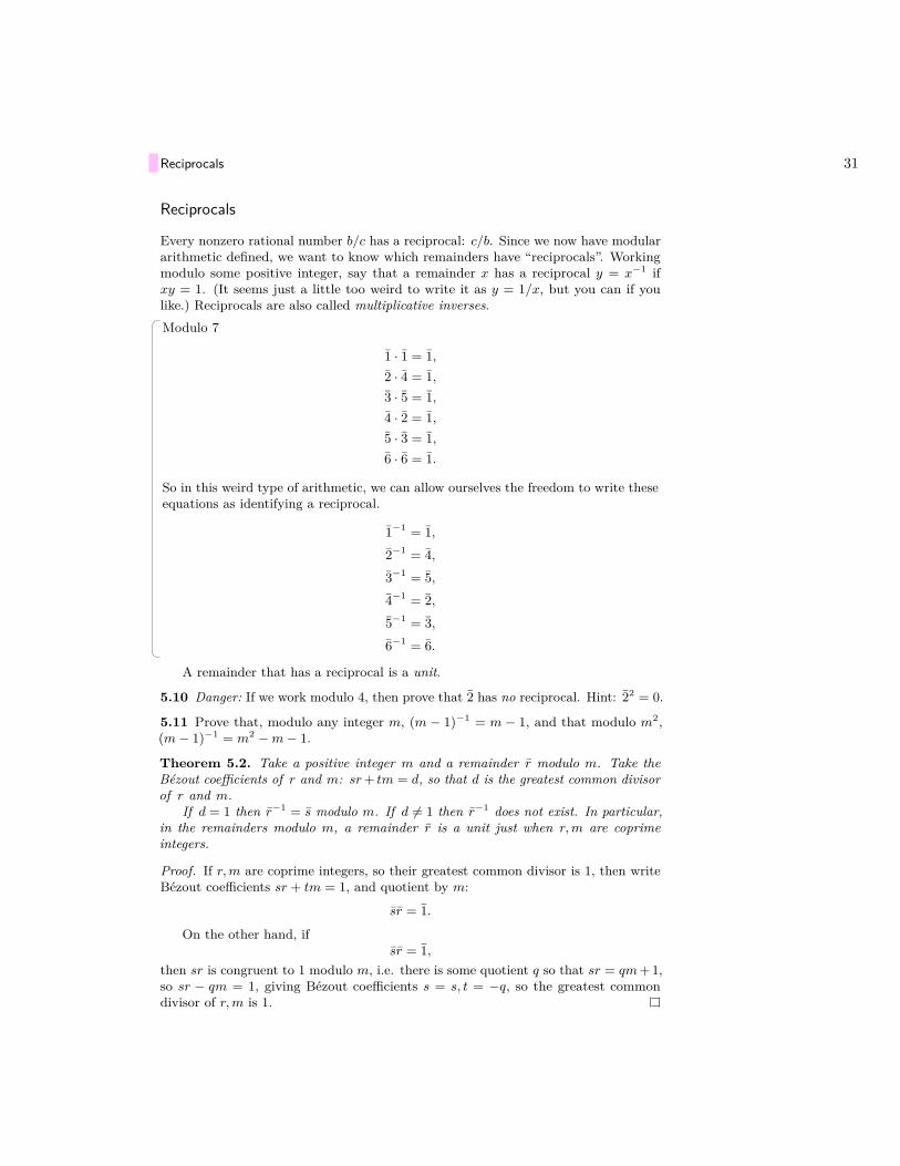
Reciprocals

Every nonzero rational number b/c has a reciprocal: c/b. Since we now have modulararithmetic defined, we want to know which remainders have “reciprocals”. Workingmodulo some positive integer, say that a remainder x has a reciprocal y = x−1 ifxy = 1. (It seems just a little too weird to write it as y = 1/x, but you can if youlike.) Reciprocals are also called multiplicative inverses.Modulo 7

1 · 1 = 1,2 · 4 = 1,3 · 5 = 1,4 · 2 = 1,5 · 3 = 1,6 · 6 = 1.

So in this weird type of arithmetic, we can allow ourselves the freedom to write theseequations as identifying a reciprocal.

1−1 = 1,2−1 = 4,3−1 = 5,4−1 = 2,5−1 = 3,6−1 = 6.

A remainder that has a reciprocal is a unit.

5.10 Danger: If we work modulo 4, then prove that 2 has no reciprocal. Hint: 22 = 0.

5.11 Prove that, modulo any integer m, (m − 1)−1 = m − 1, and that modulo m2,(m− 1)−1 = m2 −m− 1.

Theorem 5.2. Take a positive integer m and a remainder r modulo m. Take theBézout coefficients of r and m: sr+ tm = d, so that d is the greatest common divisorof r and m.

If d = 1 then r−1 = s modulo m. If d 6= 1 then r−1 does not exist. In particular,in the remainders modulo m, a remainder r is a unit just when r,m are coprimeintegers.

Proof. If r,m are coprime integers, so their greatest common divisor is 1, then writeBézout coefficients sr + tm = 1, and quotient by m:

sr = 1.

On the other hand, ifsr = 1,

then sr is congruent to 1 modulo m, i.e. there is some quotient q so that sr = qm+ 1,so sr − qm = 1, giving Bézout coefficients s = s, t = −q, so the greatest commondivisor of r,m is 1.

32 Modular arithmetic

Working modulo 163, let’s compute 14−1. First we carry out the long division

1114)

16314023149

Now let’s start looking for Bézout coefficients, by writing out matrix:(1 0 140 1 163

)and then add −11 · row 1 to row 2:(

1 0 14−11 1 9

).

Add −row 2 to row 1: (12 −1 5−11 1 9

).

Add −row 1 to row 2: (12 −1 5−23 2 4

).

Add −row 2 to row 1: (35 −3 1−23 2 4

).

Add −4 · row 1 to row 2: (35 −3 1−163 14 0

).

Summing it all up: 35 · 14 + (−3) · 163 = 1. Quotient out by 163: modulo 163,35 · 14 = 1, so modulo 163, 14−1 = 35.

5.12 Use this method to find reciprocals:a. 13−1 modulo 59b. 10−1 modulo 11c. 2−1 modulo 193.d. 6003722857−1 modulo 77695236973.

5.13 Suppose that b, c are remainders modulo a prime. Prove that bc = 0 just wheneither b = 0 or c = 0.

5.14 Suppose that p is a prime number and n is an integer with n < p. Explain why,modulo p, the numbers 0, n, 2n, 3n, . . . , (p − 1)n consist in precisely the remainders0, 1, 2, . . . , p − 1, in some order. (Hint: use the reciprocal of n.) Next, since everynonzero remainder has a reciprocal remainder, explain why the product of the nonzeroremainders is 1. Use this to explain why

np−1 ≡ 1 (mod p).

The Chinese remainder theorem 33

Finally, explain why, for any integer k,

kp ≡ k (mod p).

The Chinese remainder theoremAn old woman goes to market and a horse steps on her basket andcrushes the eggs. The rider offers to pay for the damages and asksher how many eggs she had brought. She does not remember the exactnumber, but when she had taken them out two at a time, there was oneegg left. The same happened when she picked them out three, four, five,and six at a time, but when she took them seven at a time, there werenone left. What is the smallest number of eggs she could have had?

— Brahmagupta (580CE–670CE)Brahma-Sphuta-Siddhanta (Brahma’s Correct Sys-tem)

Take a look at some numbers and their remainders modulo 3 and 5:

n nmod 3 nmod 5

0 0 01 1 12 2 23 0 34 1 45 2 06 0 17 1 28 2 39 0 4

10 1 011 2 112 0 213 1 314 2 415 0 0

Remainders modulo 3 repeat every 3, and remainders modulo 5 repeat every 5, butthe pair of remainders modulo 3 and 5 together repeat every 15.

How can you find an integer x so that

x ≡ 1 (mod 3),x ≡ 2 (mod 4),x ≡ 1 (mod 7)?

34 Modular arithmetic

A recipe: how to find an unknown integer x given only the knowledge of its remaindersmodulo various integers. Suppose we know x has remainder r1 modulom1, r2 modulom2, and so on. Let

m ..= m1m2 . . .mn.

For each i, letui ..= m

mi= m1m2 . . .mi−1mi+1mi+2 . . .mn.

Each ui has some reciprocal modulo mi, given as the remainder of some integer vi.Let

x ..= r1u1v1 + r2u2v2 + · · ·+ rnunvn.

We can simplify this a little: add or subtract multiples of m until x is in the range0 ≤ x ≤ m− 1.

Theorem 5.3. Take some positive integers m1,m2, . . . ,mn, so that any two of themare coprime. Suppose that we want to find an unknown integer x given only theknowledge of its remainders modulo m1,m2, . . . ,mn; so we know its remainder modulom1 is r1, modulo m2 is r2, and so on. There is such an integer x, given by the recipeabove, and x is unique modulo

m1m2 . . .mn.

Proof. All ofm1,m2, . . . ,mn divide ui, exceptmi. So if j 6= i then modulomj , ui = 0.All of the other mj are coprime to mi, so their product is coprime to mi, so has areciprocal modulo mi. Thus modulo mi, ui 6= 0. Then modulo mi, x = ri, and soon. So the recipe gives the required integer x. If there are two, then their differencevanishes modulo all of the mi, so is a multiple of every one of the mi, which arecoprime, so is a multiple of their product m.

Let’s find an integer x so that

x ≡ 1 (mod 3),x ≡ 2 (mod 4),x ≡ 1 (mod 7).

So in this problem we have to work modulo (m1,m2,m3) = (3, 4, 7), and get remain-ders (r1, r2, r3) = (1, 2, 1). First, no matter what the remainders, we have to workout the reciprocal mod each mi of the product of all of the other mj . So let’s reducethese products down to their remainders:

4 · 7 = 28 = 9 · 3 + 1 ≡ 1 (mod 3),3 · 7 = 21 = 5 · 4 + 1 ≡ 1 (mod 4),3 · 4 = 12 = 1 · 7 + 5 ≡ 5 (mod 7).

We need the reciprocals of these, which, to save ink, we just write down for youwithout writing out the calculations:

1−1 ≡ 1 (mod 3),1−1 ≡ 1 (mod 4),5−1 ≡ 3 (mod 7).

The Chinese remainder theorem 35

(You can easily check those.) Finally, we add up remainder times product timesreciprocal:

x = r1 · 4 · 7 · 1 + r2 · 3 · 7 · 1 + r3 · 3 · 4 · 3,= 1 · 4 · 7 · 1 + 2 · 3 · 7 · 1 + 1 · 3 · 4 · 3,= 106.

We can now check to be sure:

106 ≡ 1 (mod 3),106 ≡ 2 (mod 4),106 ≡ 1 (mod 7).

The Chinese remainder theorem tells us also that 106 is the unique solution modulo3 · 4 · 7 = 84. But then 106− 84 = 22 is also a solution, the smallest positive solution.

5.15 Solve the problem about eggs. Hint: ignore the information about eggs takenout six at a time.

5.16 Use the Chinese remainder theorem to determine the smallest number of soldierspossible in Han Xin’s army if the following facts are true. When they parade in rowsof 3 soldiers, two soldiers will be left. When they parade in rows of 5, 3 will be left,and in rows of 7, 2 will be left.

5.17 Use the Chinese remainder theorem to determine the smallest number of soldierspossible in Han Xin’s army if the following facts are true. When they parade in rowsof 3 soldiers, one soldier will be left. When they parade in rows of 7, 2 will be left,and in rows of 19, three will be left.

Given some integersm1,m2, . . . ,mn, we consider sequences (b1, b2, . . . , bn) consist-ing of remainders: b1 a remainder modulom1, and so on. Add sequences of remaindersin the obvious way:

(b1, b2, . . . , bn) + (c1, c2, . . . , cn) = (b1 + c1, b2 + c2, . . . , bn + cn) .

Similarly, we can subtract and multiply sequences of remainders:

(b1, b2, . . . , bn) (c1, c2, . . . , cn) = (b1c1, b2c2, . . . , bncn) ,

by multiplying remainders as usual, modulo the various m1,m2, . . . ,mn.

Modulo (3, 5), we multiply

(2, 4)(3, 2) = (2 · 3, 4 · 2),= (6, 8),= (0, 3).

Let m ..= m1m2 . . .mn. To each remainder modulo m, say b, associate its re-mainder b1 modulo m1, b2 modulo m2, and so on. Associate the sequence ~b ..=(b1, b2, . . . , bn) of all of those remainders. In this way we make a map taking eachremainder b modulo m to its sequence ~b of remainders modulo all of the various mi.Moreover,

−−→b+ c = ~b+~c and

−−→b− c = ~b−~c and

−→bc = ~b~c, since each of these works when

we take remainder modulo anything.

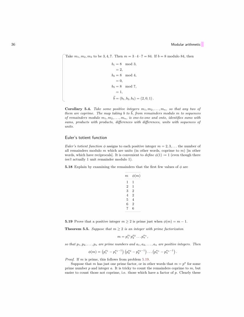
36 Modular arithmetic

Take m1,m2,m3 to be 3, 4, 7. Then m = 3 · 4 · 7 = 84. If b = 8 modulo 84, then

b1 = 8 mod 3,= 2,

b2 = 8 mod 4,= 0,

b3 = 8 mod 7,= 1,

~b = (b1, b2, b3) = (2, 0, 1) .

Corollary 5.4. Take some positive integers m1,m2, . . . ,mn, so that any two ofthem are coprime. The map taking b to ~b, from remainders modulo m to sequencesof remainders modulo m1,m2, . . . ,mn, is one-to-one and onto, identifies sums withsums, products with products, differences with differences, units with sequences ofunits.

Euler’s totient function

Euler’s totient function φ assigns to each positive integer m = 2, 3, . . . the number ofall remainders modulo m which are units (in other words, coprime to m) [in otherwords, which have reciprocals]. It is convenient to define φ(1) ..= 1 (even though thereisn’t actually 1 unit remainder modulo 1).

5.18 Explain by examining the remainders that the first few values of φ are

m φ(m)

1 12 13 24 25 46 27 6

5.19 Prove that a positive integer m ≥ 2 is prime just when φ(m) = m− 1.

Theorem 5.5. Suppose that m ≥ 2 is an integer with prime factorizaton

m = pa11 pa2

2 . . . pann ,

so that p1, p2, . . . , pn are prime numbers and a1, a2, . . . , an are positive integers. Then

φ(m) =(pa1

1 − pa1−11

) (pa2

2 − pa2−12

). . .(pann − pan−1

n

).

Proof. If m is prime, this follows from problem 5.19.Suppose that m has just one prime factor, or in other words that m = pa for some

prime number p and integer a. It is tricky to count the remainders coprime to m, buteasier to count those not coprime, i.e. those which have a factor of p. Clearly these

Euler’s totient function 37

are the multiples of p between 0 and pa − p, so the numbers pj for 0 ≤ j ≤ pa−1 − 1.So there are pa−1 such remainders. We take these out and we are left with pa − pa−1

remainders left, i.e. coprime.If b, c are coprime integers ≥ 2, then corollary 5.4 on the preceding page maps

units modulo bc to pairs of a unit modulo b and a unit modulo c, and is one-to-oneand onto. Therefore counting units: φ(bc) = φ(b)φ(c).

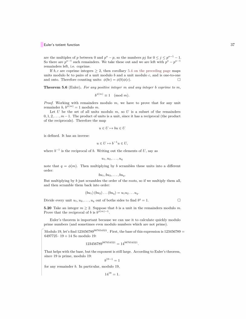
Theorem 5.6 (Euler). For any positive integer m and any integer b coprime to m,

bφ(m) ≡ 1 (mod m).

Proof. Working with remainders modulo m, we have to prove that for any unitremainder b, bφ(m) = 1 modulo m.

Let U be the set of all units modulo m, so U is a subset of the remainders0, 1, 2, . . . ,m− 1. The product of units is a unit, since it has a reciprocal (the productof the reciprocals). Therefore the map

u ∈ U 7→ bu ∈ U

is defined. It has an inverse:

u ∈ U 7→ b−1u ∈ U,

where b−1 is the reciprocal of b. Writing out the elements of U , say as

u1, u2, . . . , uq

note that q = φ(m). Then multiplying by b scrambles these units into a differentorder:

bu1, bu2, . . . , buq.

But multiplying by b just scrambles the order of the roots, so if we multiply them all,and then scramble them back into order:

(bu1) (bu2) . . . (buq) = u1u2 . . . uq.

Divide every unit u1, u2, . . . , uq out of boths sides to find bq = 1.

5.20 Take an integer m ≥ 2. Suppose that b is a unit in the remainders modulo m.Prove that the reciprocal of b is bφ(m)−1.

Euler’s theorem is important because we can use it to calculate quickly moduloprime numbers (and sometimes even modulo numbers which are not prime).

Modulo 19, let’s find 123456789987654321. First, the base of this expression is 123456789 =6497725 · 19 + 14 So modulo 19:

123456789987654321 = 14987654321.

That helps with the base, but the exponent is still large. According to Euler’s theorem,since 19 is prime, modulo 19:

b19−1 = 1for any remainder b. In particular, modulo 19,

1418 = 1.

38 Modular arithmetic

So every time we get rid of 18 copies of 14 multiplied together, we don’t change ourresult. Divide 18 into the exponent:

987654321 = 54869684 · 18 + 9.

So then modulo 19:14987654321 = 149.

We leave the reader to check that 149 = 18 modulo 19, so that finally, modulo 19,

123456789987654321 = 18.

5.21 By hand, using Euler’s totient function, compute 127162 modulo 120.

Lemma 5.7. For any prime number p and integers b and k, b1+k(p−1) = b modulo p.

Proof. If b is a multiple of p then b = 0 modulo p so both sides are zero. If b is nota multiple of p then bp−1 = 1 modulo p, by Euler’s theorem. Take both sides to thepower k and multiply by b to get the result.

Theorem 5.8. Suppose that m = p1p2 . . . pn is a product of distinct prime numbers.Then for any integers b and k with k ≥ 0,

b1+kφ(m) ≡ b (mod m).

Proof. By lemma 5.7, the result is true ifm is prime. So if we take two prime numbersp and q, thenb1+k(p−1)(q−1) = b modulo p, but also modulo q, and therefore modulopq. The same trick works if we start throwing in more distinct prime factors intom.

5.22 Give an example of integers b and m with m ≥ 2 for which b1+φ(m) 6= b modulom.

Sage

In Sage, the quotient of 71 modulo 13 is mod(71,13). The tricky bit: it returns a“remainder modulo 13”, so if we write

a=mod(71,13)

this will define a to be a “remainder modulo 13”. The value of a is then 6, but thevalue of a2 is 10, because the result is again calculated modulo 13.

Euler’s totient function is

euler_phi(777)

which yields φ(777) = 432. To find 14−1 modulo 19,

inverse_mod(14,19)

yields 14−1 = 15 modulo 19.We can write our own version of Euler’s totient function, just to see how it might

look:

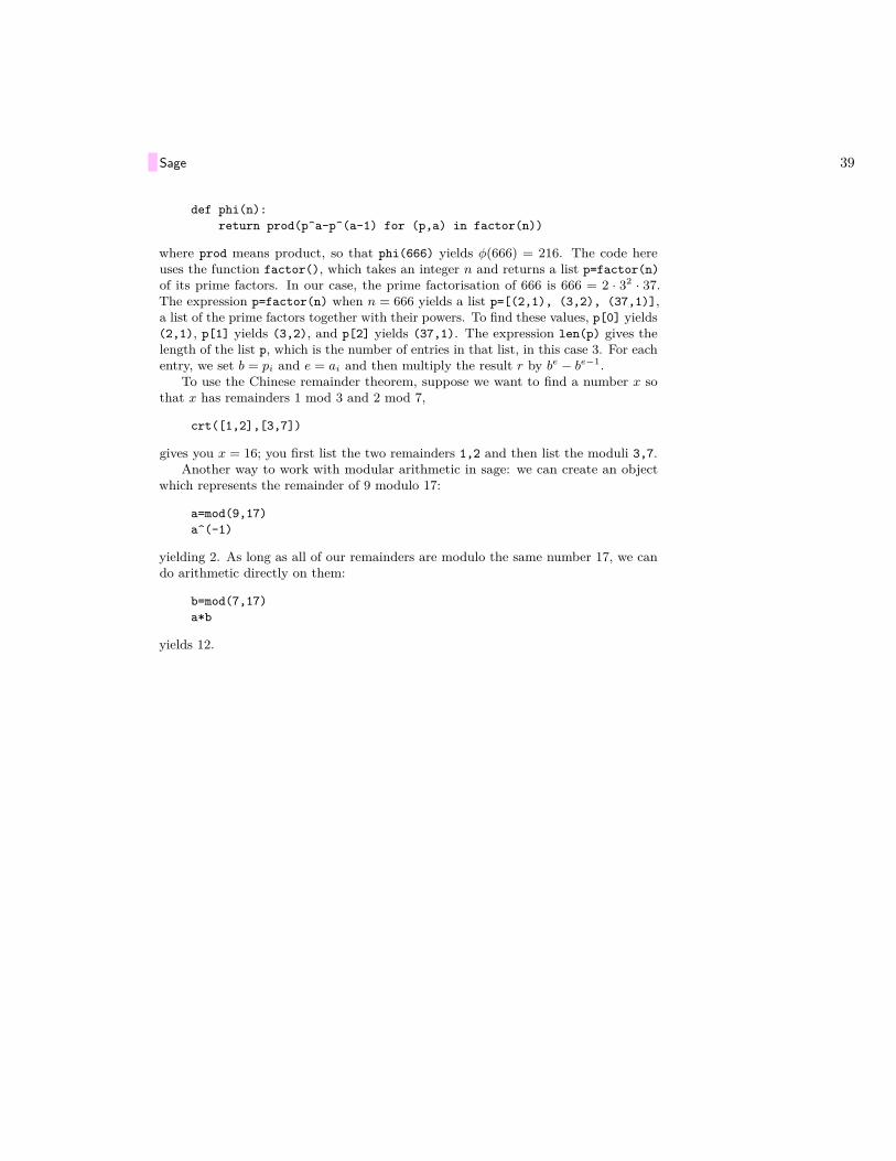
Sage 39

def phi(n):return prod(p^a-p^(a-1) for (p,a) in factor(n))

where prod means product, so that phi(666) yields φ(666) = 216. The code hereuses the function factor(), which takes an integer n and returns a list p=factor(n)of its prime factors. In our case, the prime factorisation of 666 is 666 = 2 · 32 · 37.The expression p=factor(n) when n = 666 yields a list p=[(2,1), (3,2), (37,1)],a list of the prime factors together with their powers. To find these values, p[0] yields(2,1), p[1] yields (3,2), and p[2] yields (37,1). The expression len(p) gives thelength of the list p, which is the number of entries in that list, in this case 3. For eachentry, we set b = pi and e = ai and then multiply the result r by be − be−1.

To use the Chinese remainder theorem, suppose we want to find a number x sothat x has remainders 1 mod 3 and 2 mod 7,

crt([1,2],[3,7])

gives you x = 16; you first list the two remainders 1,2 and then list the moduli 3,7.Another way to work with modular arithmetic in sage: we can create an object

which represents the remainder of 9 modulo 17:

a=mod(9,17)a^(-1)

yielding 2. As long as all of our remainders are modulo the same number 17, we cando arithmetic directly on them:

b=mod(7,17)a*b

yields 12.

Chapter 6

Secret messages

And when at last you find someone to whom you feel you can pourout your soul, you stop in shock at the words you utter— theyare so rusty, so ugly, so meaningless and feeble from being keptin the small cramped dark inside you so long.

— Sylvia PlathThe Unabridged Journals of Sylvia Plath

Man is not what he thinks he is, he is what he hides.

— André Malraux

Enigma, Nazi secret code machine

41

42 Secret messages

RSA: the Cocks, Rivest, Shamir and Adleman algorithm

Alice wants to send a message to Bob, but she doesn’t want Eve to read it. Shefirst writes the message down in a computer, as a collection of 0’s and 1’s. She canthink of these 0’s and 1’s as binary digits of some large integer x, or as binary digitsof some remainder x modulo some large integer m. Alice takes her message x andturns it into a secret coded message by sending Bob not the original x, but insteadsending him xd modulo m, for some integer d. This will scramble up the digits ofx unrecognizably, if d is chosen “at random”. For random enough d, and suitablychosen positive integer m, Bob can unscramble the digits of xd to find x.

For example, take m ..= 55 and let d ..= 17 and y ..= x17 mod 55:

x y x y x y x y

0 0 14 9 28 8 42 371 1 15 5 29 39 43 432 7 16 36 30 35 44 443 53 17 52 31 26 45 454 49 18 28 32 32 46 515 25 19 24 33 33 47 426 41 20 15 34 34 48 387 17 21 21 35 40 49 148 13 22 22 36 31 50 309 4 23 23 37 27 51 6

10 10 24 29 38 3 52 211 11 25 20 39 19 53 4812 12 26 16 40 50 54 5413 18 27 47 41 46 55 0

If Alice sends Bob the secret message y = x17, then Bob decodes it by x = y33, aswe will see.

Theorem 6.1. Pick two different prime numbers p and q and let m ..= pq. RecallEuler’s totient function φ(m). Suppose that d and e are positive integers so that de = 1modulo φ(m). If Alice maps each remainder x to y = xd modulo m, then Bob caninvert this map by taking each remainder y to x = ye modulo m.

Proof. We have to prove that(xd)e = x modulo m for all x, i.e. that xde = x modulo

m for all x. For x coprime to m, this follows from Euler’s theorem, but for othervalues of x the result is not obvious.

By theorem 5.5 on page 36, φ(m) = (p − 1)(q − 1). Since de = 1 modulo φ(m),clearly

de− 1 = k(p− 1)(q − 1)

for some integer k. If k = 0, then de = 1 and the result is clear: x1 = x. Since d ande are positive integers, de− 1 is not negative, so k ≥ 0. So we can assume that k > 0.The result follows from theorem 5.8 on page 38.

Sage 43

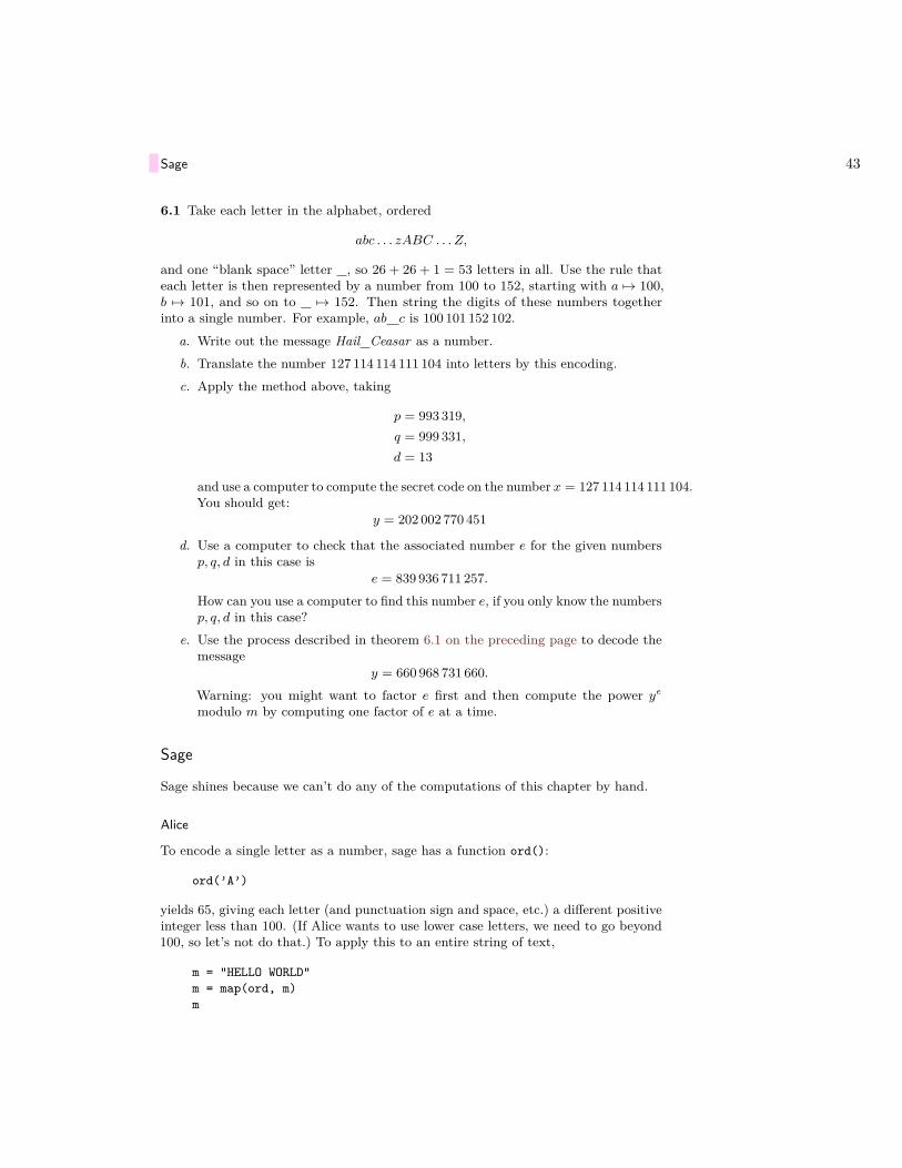
6.1 Take each letter in the alphabet, ordered

abc . . . zABC . . . Z,

and one “blank space” letter , so 26 + 26 + 1 = 53 letters in all. Use the rule thateach letter is then represented by a number from 100 to 152, starting with a 7→ 100,b 7→ 101, and so on to 7→ 152. Then string the digits of these numbers togetherinto a single number. For example, ab c is 100 101 152 102.

a. Write out the message Hail Ceasar as a number.b. Translate the number 127 114 114 111 104 into letters by this encoding.c. Apply the method above, taking

p = 993 319,q = 999 331,d = 13

and use a computer to compute the secret code on the number x = 127 114 114 111 104.You should get:

y = 202 002 770 451

d. Use a computer to check that the associated number e for the given numbersp, q, d in this case is

e = 839 936 711 257.How can you use a computer to find this number e, if you only know the numbersp, q, d in this case?

e. Use the process described in theorem 6.1 on the preceding page to decode themessage

y = 660 968 731 660.Warning: you might want to factor e first and then compute the power yemodulo m by computing one factor of e at a time.

Sage

Sage shines because we can’t do any of the computations of this chapter by hand.

Alice

To encode a single letter as a number, sage has a function ord():

ord(’A’)

yields 65, giving each letter (and punctuation sign and space, etc.) a different positiveinteger less than 100. (If Alice wants to use lower case letters, we need to go beyond100, so let’s not do that.) To apply this to an entire string of text,

m = "HELLO WORLD"m = map(ord, m)m

44 Secret messages

yields [72, 69, 76, 76, 79, 32, 87, 79, 82, 76, 68]. Alice turns this list of numbers into asingle number, by first reversing order:

m.reverse()m

yields [68, 76, 82, 79, 87, 32, 79, 76, 76, 69, 72]. Then the expression

ZZ(m,100)

adds up successively these numbers, multiplying by 100 at each step, so that

x=ZZ(m,100)x

yields x. This is the integer Alice wants to encode. Alice sets up the values of herprimes and exponent:

p=993319q=999331d=13m=p*qf=euler_phi(m)e=inverse_mod(d,f)

The secret code Alice sends is y = xd (mod m). Sage can compute powers in modulararithmetic quickly (using the same tricks we learned previously):

y=power_mod(x, d, m)y

yielding 782102149108. This is Alice’s encoded message. She can send it to Bobopenly: over the phone, by email, or on a billboard.

Bob

Bob decodes by

x=power_mod(y, e, m)x

yielding 53800826153. (Alice has secretly whispered e and m to Bob.) Bob turns thisnumber x back into text by using the function chr(), which is the inverse of ord():

def recover_message(x):if x==0:

return ""else:

return recover_message(x//100)+chr(x%100)

Bob applies this:

print(recover_message(x))

to yield HELLO WORLD.

Chapter 7

Rational, real and complex numbers

A fragment of the Rhind papyrus, 1650BCE, containing ancient Egyptian calculationsusing rational numbers

There is a remote tribe that worships the number zero. Is nothing sacred?

— Les Dawson

Rational numbers

A rational number is a ratio of two integers, like

23 ,

−79 ,

22−11 ,

02 .

45

46 Rational, real and complex numbers

We also write them 2/3,−7/9, 22/−11, 0/2. In writing 23 , the number 2 is the nu-

merator , and 3 is the denominator . We can think of rational numbers two differentways:

a. Geometry: Divide up an interval of length b into c equal pieces. Each piece haslength b/c.

b. Algebra: a rational number b/c is just a formal expression we write down, withtwo integers b and c, in which c 6= 0. We agree that any rational number b

cis

equal to abac

for any integer a 6= 0.

Of course, the two ideas give the same objects, but in these notes, the algebra approachis best. For example, we see that 22/11 = 14/7, because I can factor out:

2211 = 11 · 2

11 · 1 ,

and factor out147 = 7 · 2

7 · 1 .

Write any rational number b1 as simply b, and in this way see the integers sitting

among the rational numbers.More generally, any rational number b/c can be simplified by dividing b and c by

their greatest common divisor, and then changing the sign of b and of c if needed, toensure that c > 0; the resulting rational number is in lowest terms.

7.1 Bring these rational numbers to lowest terms: 224/82, 324/− 72, −1000/8800.

Multiply rational numbers by

b

c

B

C= bB

cC.

Similarly, divide a rational number by a nonzero rational number as

bcBC

= b

c

C

B.

Add rationals with the same denominator as:

b

d+ c

d= b+ c

d.

The same for subtraction:b

d− c

d= b− c

d.

But if the denominators don’t match up, we rescale to make them match up:

b

c+ B

C= bC

cC+ cB

cC.

7.2 If we replace bcby ab

acand we replace B

Cby AB

AC, for some nonzero integers a,A,

prove that the result of computing out bc

+ BC, bc− B

Cor b

cBC

only changes by scalingboth numerator and denominator by the same nonzero integer. Hence the arithmeticoperations don’t contradict our agreement that we declare b

cto equal ab

ac.

Real numbers 47

7.3 By hand, showing your work, simplify

23 −

12 ,

32449 ·

39281 ,

45 + 7

4 .

Lemma 7.1. The number√

2 is irrational. (To be more precise, no rational numbersquares to 2.)

Proof. If it is rational, say√

2 = bc, then c

√2 = b, so squaring gives c2 · 2 = b2. Every

prime factor in b occurs twice in b2, so the prime factorization of the right hand sidehas an even number of factors of each prime. But the left hand side has an oddnumber of factors of 2, since c2 has an even number, but there is another factor of 2on the left hand side. This contradicts uniqueness of prime factorization.

7.4 Suppose that N is a positive integer. Prove that either√N is irrational or N is

a perfect square, i.e. N = n2 for some integer n.

7.5 Prove that there are no rational numbers x and y satisfying√

3 = x+ y√

2.

A rational number is positive if it is a ratio of positive integers. We write x > yto mean that x− y is positive, and similarly define x < y, x ≤ y, and so on.

7.6 Prove that every positive rational number has a unique expression in the form

pα11 pα2

2 . . . pαkk

qβ11 qβ2

2 . . . qβ``

wherep1, p2, . . . , pk, q1, q2, . . . , q`

are prime numbers, all different, with p1 < p2 < · · · < pk and q1 < q2 < · · · < q` and

α1, α2, . . . , αk, β1, β2, . . . , β`

are positive integers. For example

23416 = 32 · 13

23 .

7.7 Of the various laws of addition and multiplication and signs for integers, whichhold true also for rational numbers?

The most important property that rational numbers have, that integers don’t, isthat we can divide any rational number by any nonzero rational number.

Real numbersOrder is an exotic in Ireland. It has been imported from England butwill not grow. It suits neither soil nor climate.

— J.A. Froude

48 Rational, real and complex numbers

Think of the rational numbers geometrically, so that b/c is the length of each piecewhen a rod of length b is cut into c equal lengths. Draw an straight line, infinite inboth directions, and mark a point 0 on it. Then mark at point 1 at 1 unit of distancefrom 0, and so on marking all of the integers to form a number line. The points of thiscontinuous number line are the real numbers. This physical definition doesn’t makeit possible to prove anything about the real numbers.

The rational numbers are insufficient for algebra: they have no√

2. Imaginetaking all positive rational numbers b/c for which b2/c2 > 2. Thinking geometrically,drawing a number line:

√2

Our rational numbers sit along the line getting very close to the circled point of theline, which should be the point

√2. But there is no rational number there. From

now on, we assume that the reader is familiar with the real numbers and their basicproperties; see [6] for the complete story of real numbers.

Complex numbers

Entre deux vérités du domaine réel, le chemin le plus facile et le pluscourt passe bien souvent par le domaine complexe.The shortest and easiest path between any two facts about the realdomain often passes through the complex domain.

— Paul PainlevéAnalyse des travaux scientifiques

Just as the rational numbers have a deficiency, no√

2, so the real numbers have adeficiency: no

√−1. We can fix this by introducing the complex numbers. Here are

two definitions:a. Algebra: We agree to play a game, where we write down algebraic expressions in

real numbers and in an abstract variable i, but we treat the symbol i accordingto the following rule. Whenever we see two copies of i multiplied together (orwe see i2) appear anywhere, we are allowed to wipe them out and replace with−1, and vice versa when we see a −1 we can replace it with an i2. We force byhand the existence of a

√−1 by forcing the abstract symbol i to be

√−1.

b. Geometry: We draw the usual x, y axes on the plane. We pretend that eachpoint of the plane represents a single number, which we write as z = x+ yi torepresent the point (x, y). If we have two points, z = x+ yi and Z = X + Y i,we add them by the rule:

z + Z = (x+X) + (y + Y )i

and multiply them by the rule:

zZ = (xX − yY ) + (xY + yX)i.

For example,

(2 + 4i)(3− i) = (2 · 3 + 4 · 1) + (−2 + 4 · 3)i = 10 + 10i.

Sage 49

It isn’t at all clear that these two games we can play arrive at the same result. Notethat the rule for multiplication seems to come out of the air in the geometric theory,but in the algebraic theory it is just what you get by expanding out both sides andinsisting that i2 = −1. Algebra is in this respect clearly superior. But the geometricapproach makes very precise what sort of objects we are really dealing with, so wewill use it as our definition.

Just like with rational numbers, if a complex number z = x+ yi is not zero, or inother words x and y are not both zero, then it has a reciprocal

1z

= x− yix2 + y2 .

7.8 Check that this is a reciprocal. Why is it defined?

Complex conjugation is the operation taking z = x+ yi to z ..= x− iy.

7.9 Prove that a complex number z is a real number just when z = z.

7.10 Prove that addition, subtraction, multiplication and division of complex numberspasses through conjugation:

z + w = z + w,

z − w = z − w,zw = z w,(z

w

)= z

w,

for any complex numbers z and w. Explain by induction why, for any polynomial p(z)with real number coefficients,

p(z) = p(z) ,for any complex number z.

The norm or modulus of a complex number z = x+ yi is the real number |z| ..=√x2 + y2.

7.11 Prove that zz = |z| for any complex number z.

Sage

Sage represents numbers in two different ways: as exact symbolic expressions, or as afinite decimal approximation (often called a numeric or floating point representation).For example we compute 7

2 + 53 symbolically as

7/2+5/3

yielding 316 . We can also play with irrational numbers symbolically: represent

√27 as

sqrt(27)

which sage simplifies to yield 3√

3.We will never use decimal approximations in this class (please don’t), but here is

how you can use them if you wish. By writing out a number with a decimal point, weare asking sage to approximate numerically, keeping only some number of decimalsaccuracy:

50 Rational, real and complex numbers

sqrt(27.0)

yields 5.19615242270663. If we want to ask sage to give us a particular number ofdecimal places accuracy in a decimal approximation of a symbolic expression, say 50decimals:

numerical_approx(pi, digits=50)

yields3.1415926535897932384626433832795028841971693993751.

To use complex numbers, try

z=3+4*ireal_part(z)

yielding 3, the real part, while imag_part(z) yields 4.

Chapter 8

Polynomials

I was x years old in the year x2.— Augustus De Morgan (when asked his age)

A polynomial in a variable x is an expression like

1, x+ 1, 5 + 3x2 − 2x,

a finite sum of terms, each the product of a number (the coefficient of the term), anda nonnegative integer power of x (the degree of the term). We define the degree ofa constant to be 0, except that the degree of 0 is defined to be −∞. We can addtogether coefficients of terms of the same degree:

2x2 + 7x2 + x = (2 + 7)x2 + x = 9x2 + x.

We usually arrange that the terms decrease in degree, writing 1+5x+x2 as x2 +5x+1.When we write a polynomial this way, the degree is the largest degree of any term. Wemight ask the coefficients to be integers, rational numbers, real numbers, or complexnumbers (in which case, we usually use z as the name of the variable, instead ofx). Bizarrely, we might even allow the coefficients to be remainders modulo someinteger. As soon as we fix on any of these choices of coefficients, the addition laws,multiplication laws, and distributive law (familiar from chapter 1) are immediatelyobvious, just writing b(x) as a polynomial, instead of an integer b, and so on, andchanging the word integer to polynomial. We will ignore the sign laws and the law ofwell ordering.

Let’s work modulo 2, in honour of George Boole. Let p(x) ..= x2 +x. We write x2 +xto mean 1x2 + 1x, i.e. the coefficients are remainders. This polynomial is not zero,because its coefficients are not zero. Danger: if we ask that x also be a remaindermodulo 2, we might want to think of this polynomial as a function of a variable x.But then that function is zero, because if we let x = 0 then

p(0)

= 1 · 02 + 1 · 0 = 0

and if we let x = 1 thenp(1)

= 1 · 12 + 1 · 1 = 0modulo 2. So a polynomial with coefficients in remainders modulo an integer is notjust a function. It is a purely algebraic object.

8.1 Work modulo 5: for which remainders a can we find a remainder b so that a = b2?In other words, which elements have square roots?

51

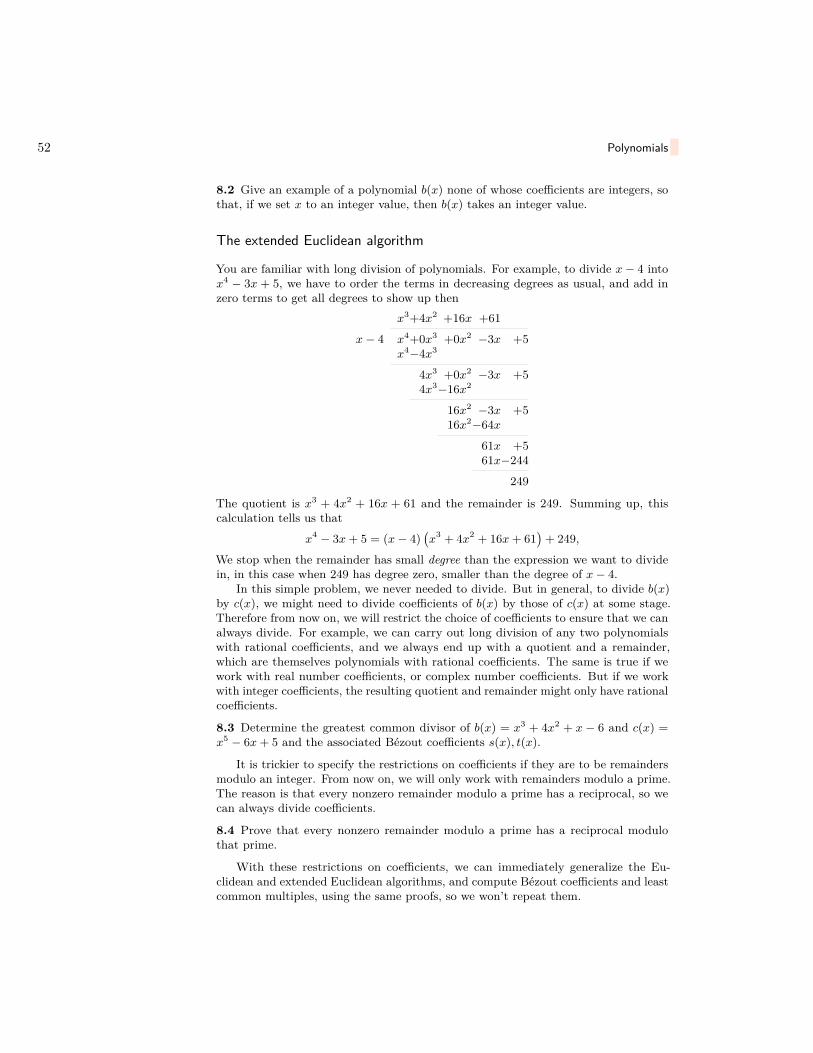
52 Polynomials

8.2 Give an example of a polynomial b(x) none of whose coefficients are integers, sothat, if we set x to an integer value, then b(x) takes an integer value.

The extended Euclidean algorithm

You are familiar with long division of polynomials. For example, to divide x− 4 intox4 − 3x + 5, we have to order the terms in decreasing degrees as usual, and add inzero terms to get all degrees to show up then

x3+4x2 +16x +61

x− 4 x4+0x3 +0x2 −3x +5x4−4x3

4x3 +0x2 −3x +54x3−16x2

16x2 −3x +516x2−64x

61x +561x−244

249

The quotient is x3 + 4x2 + 16x + 61 and the remainder is 249. Summing up, thiscalculation tells us that

x4 − 3x+ 5 = (x− 4)(x3 + 4x2 + 16x+ 61

)+ 249,

We stop when the remainder has small degree than the expression we want to dividein, in this case when 249 has degree zero, smaller than the degree of x− 4.

In this simple problem, we never needed to divide. But in general, to divide b(x)by c(x), we might need to divide coefficients of b(x) by those of c(x) at some stage.Therefore from now on, we will restrict the choice of coefficients to ensure that we canalways divide. For example, we can carry out long division of any two polynomialswith rational coefficients, and we always end up with a quotient and a remainder,which are themselves polynomials with rational coefficients. The same is true if wework with real number coefficients, or complex number coefficients. But if we workwith integer coefficients, the resulting quotient and remainder might only have rationalcoefficients.

8.3 Determine the greatest common divisor of b(x) = x3 + 4x2 + x − 6 and c(x) =x5 − 6x+ 5 and the associated Bézout coefficients s(x), t(x).

It is trickier to specify the restrictions on coefficients if they are to be remaindersmodulo an integer. From now on, we will only work with remainders modulo a prime.The reason is that every nonzero remainder modulo a prime has a reciprocal, so wecan always divide coefficients.

8.4 Prove that every nonzero remainder modulo a prime has a reciprocal modulothat prime.

With these restrictions on coefficients, we can immediately generalize the Eu-clidean and extended Euclidean algorithms, and compute Bézout coefficients and leastcommon multiples, using the same proofs, so we won’t repeat them.

The extended Euclidean algorithm 53

Take the polynomials b(x) = 3 + 2x− x2 and c(x) = 12− x− x2. We want to findthe Bézout coefficients and the greatest common divisor among polynomials over therational numbers. At each step, force down the degree of one of the polynomials.(

1 0 3 + 2x− x2

0 1 12− x− x2

)add -row 2 to row 1,(

1 −1 −9 + 3x0 1 12− x− x2

)add (x/3)row 1 to row 2,(

1 −1 −9 + 3xx3 1− x

3 12− 4x

)add 4

3 row 1 to row 2,(1 −1 −9 + 3x

43 + x

3 − 13 −

x3 0

)The equation of the Bézout coefficients is therefore

1(3 + 2x− x2)− 1

(12− x− x2) = −9 + 3x = 3(x− 3).

The greatest common divisor, once we divide away any coefficient in front of thehighest term, is x− 3. A monic polynomial is one whose highest order term has coef-ficient 1: the greatest common divisor will always be taken to be a monic polynomial,and then there is a unique greatest common divisor.

Fix a choice of whether we are working with rational, real or complex coefficientsor if our coefficients will be remainders modulo a prime. We will say this choice is achoice of field, and our polynomials are said to live over that field. A polynomial overa chosen field is irreducible if it does not split into a product a(x)b(x) of polynomialsover the same field, except for having a(x) or b(x) constant. The same proof forprime numbers proves that a polynomial over a field admits a factorization into aproduct of irreducibles over that field, unique up to reordering the factors and perhapsmultiplying any of the factors by a nonzero constant.

Let’s working over the remainders modulo 2. Notice that 2x = 0x = 0, and similarlythat −1 = 1 so −x2 = x2. Let’s find the Bézout coefficients of b(x) ..= x3 + x andc(x) ..= x2: (

1 0 x3 + x0 1 x2

), add x(row 2) to row 1,(

1 x x0 1 x2

), add x(row 1) to row 2,(

1 x xx x2 + 1 0

).

The Bézout coefficients are 1, x, and the greatest common divisor is x:

1(x3 + x

)+ x

(x2) = x.

54 Polynomials

Factoring

- What is a multiple root of a polynomial?- Well, it is when we substitute a number in the polynomial and getzero. Then do it again and again get zero and so k times . . . . But onthe (k + 1)-st time the zero does not appear.

— A. A. KirillovWhat are Numbers?

Proposition 8.1. Take any constant c and any polynomial p(x) over any field. Thenp(x) has remainder p(c) when divided by x− c.

Proof. Take quotient and remainder: p(x) = (x− c)q(x) + r(x), using the Euclideanalgorithm. The degree of the remainder is smaller than the degree of x − c, so theremainder is a constant, say r0. Plug in x = c: p(c) = (c− c)q(c) + r0 = r0.

A root of a polynomial p(x) is a number c in whichever field we work over so thatp(c) = 0.

Corollary 8.2. A polynomial p(x) over any field has a root at x = c, i.e. p(c) = 0,for some constant c in the field, just when the linear polynomial x−c divides into p(x).

8.5 Work over the field of real numbers, or the field of rational numbers, or the fieldof complex numbers, or the field of remainders modulo any odd prime number. Showthat the solutions of the quadratic equation

0 = ax2 + bx+ c

(where a, b, c are constants and a 6= 0) are precisely the numbers x so that(x+ b

2a

)2= b2

2a2 −c

a.

Show that every constant d has either two square roots, which we denote as ±√d, or

one square root (if 2 = 0 in our field or if d = 0) or has no square roots. Concludethat the solution of the quadratic equation, over any field, are

x = −b±√b2 − 4ac

2a .

just when the required square roots exist.

8.6 Prove that a quadratic or cubic polynomial (in other words of degree 2 or 3) overany field is reducible just when it has a root.

8.7 Prove that the polynomial x3 + x+ 1 is irreducible over the field of remaindersmodulo 2. By writing down all quadratic polynomials over that field, and factoringall of them but this one, show that this is the only irreducible quadratic polynomialover that field.

Rational roots 55

The polynomial x3 + x + 1 is irreducible over the field of remainders modulo 2, aswe saw in the previous problem. But then, if it is reducible over the integers, saya(x)b(x), then quotient out the coefficients modulo 2 to get a factorization a(x)b(x)over the field of remainders modulo 2, a contradiction. Therefore x3 + x + 1 isirreducible over the integers.

Corollary 8.3. Every polynomial over any field has at most one factorisation intolinear factors, up to reordering the factors.

Proof. The linear factors are determined by the roots. Divide off one linear factorfrom each root, and apply induction on the degree of the polynomial to see that thenumber of times each linear factor appears is uniquely determined.

8.8 Suppose that p(x) and q(x) are polynomials over some field, both of degree atmost n, and that p(c) = q(c) for n+ 1 different numbers c from the field. Prove thatp(c) = q(c) for all numbers c from the field.

8.9 Why are we working over fields? Working modulo 6, consider the polynomialb(x) = x2 + 5x. How many roots does it have among the remainders module 6? Howmany factorizations can you make for it, working modulo 6?

A root c of a polynomial p(x) has multiplicity k if (x− c)k divides p(x).

Corollary 8.4. Over any field, the degree of a polynomial is never less than the sumof the multiplicities of its roots, with equality just when the polynomial is a product oflinear factors.

Proof. Degrees add when polynomials multiply, by looking at the leading term.

Rational roots

A powerful trick for guessing rational roots of integer coefficient polynomials:

Lemma 8.5. If a polynomial p(x) with integer coefficients has a rational root x = n/d,with n and d coprime integers, then the numerator n divides the coefficient of thelowest term of p(x), while the denominator d divides the coefficient of the highestterm of p(x).

Proof. Write out

p(x) = akxk + ak−1x

k−1 + · · ·+ a1x+ a0,

so that these integers a0, a1, . . . , ak are the coefficients of p(x). Plug in:

0 = ak(n/d)k + ak−1(n/d)k−1 + · · ·+ a1(n/d) + a0.

Multiply both sides by dk:

0 = aknk + ak−1n

k−1d+ · · ·+ a1ndk−1 + a0d

k.

All terms but the last term contain a factor of n, so n divides into the last term. Butn and d are coprime, so n divides into a0. The same trick backwards: all terms butthe first term contain a factor of d, so d divides into the first term. But n and d arecoprime, so d divides into ak.

56 Polynomials

The polynomial p(x) = x3− 3x− 1, if it had a rational root n/d, would need to haven divide into −1, while d would divide into 1. So the only possibilities are n/d = 1or n/d = −1. Plug in to see that these are not roots, so x3 − 3x− 1 has no rationalroots.

8.10 Using lemma 8.5 on the preceding page, find all rational roots ofa. x2 − 5,b. x2 − 3x− 5,c. x1000 − 3x− 5.d. x2/3− x− 5/3,

Sage

To construct polynomials in a variable x, we first define the variable, using the strangeexpression:

x = var(’x’)

We can then solve polynomial equations:

solve(x^2 + 3*x + 2, x)

yielding [x == -2, x == -1]. To factor polynomials:

x=var(’x’)factor(x^2-1)

yields (x + 1)*(x - 1). To use two variables x and y:

x, y = var(’x, y’)solve([x+y==6, x-y==4], x, y)

yielding [[x == 5, y == 1]]. We can take greatest common divisor:

x=var(’x’)b=x^3+x^2c=x^2+xgcd(b,c)

yielding x2 +x. For some purposes, we will need to tell sage which field the coefficientsof our polynomials come from. We can get the quotient and remainder in polynomialdivision by

R.<x> = PolynomialRing(QQ)b=x^3+x^2c=x^2+xb.quo_rem(c)

yielding (x, 0). To find Bézout coefficients,

xgcd(x^4-x^2,x^3-x)

Interpolation 57

yields(x3 − x, 0, 1

).

The expression R.<x> = PolynomialRing(QQ) tells sage to use polynomials in avariable x with coefficients being rational numbers. The set of all rational numbers iscalled Q, written QQ when we type into a computer. To work with coefficients thatare integers modulo a prime, for example with integers modulo 5:

R.<x> = PolynomialRing(GF(5))b=x^3+x^2+1c=x^2+x+1b.quo_rem(c)

yields (x, 4x+ 1). The set of all integers modulo a prime p is sometimes called GF(p).We can define our own function to calculate Bézout coefficients, which does exactly

what the xgcd() function does on polynomials of one variable:

def bezpoly(b,c):p,q,r=1,0,bs,t,u=0,1,cwhile u<>0:

if r.degree()>u.degree():p,q,r,s,t,u=s,t,u,p,q,r

Q=u//rs,t,u=s-Q*p,t-Q*q,u-Q*r

return (r,p,q)

Then the code

R.<t> = PolynomialRing(QQ)f=(2*t+1)*(t+1)*(t-1)g=(2*t+1)*(t-1)*t^2bezpoly(f,g)

returns(2t2 − t− 1,−t+ 1, 1

).

Interpolation

Theorem 8.6. Over any field, if we specify distinct values x0, . . . , xn and arbitraryvalues y0, . . . , yn, there is a unique polynomial p(x) of degree n so that p(xi) = yi.

The polynomial p(x) interpolates the values yi at the points xi.

Proof. We associate to the numbers x0, . . . , xn the polynomials

pj(x) = (x− x0) . . . (x− xj−1)(x− xj+1) . . . (x− xn)(xj − x0) . . . (xj − xj−1)(xj − xj+1) . . . (xj − xn) .

for j = 0, 1, 2, . . . , n. The reader can check that pj(xj) = 1 while pj(xi) = 0 for i 6= j.Then

p(x) = y0p0(x) + y1p1(x) + · · ·+ ynpn(x)is our required polynomial. To check that it is unique, if there are two such polynomials,say p(x) and q(x), both of degree at most n, both equal to yi at x = xi, their differencep(x)− q(x) vanishes at x = xi, so is divisible by (x− x0)(x− x1) . . . (x− xn), whichhas degree n+ 1. But their difference has degree at most n, so is zero.

58 Polynomials

8.11 What can go wrong with interpolation if the numbers are drawn from theremainders modulo 6?

Chapter 9

Real polynomials, complex polynomials

In this chapter (and only this chapter), we assume that the reader is familiar with realnumbers, with continuity, and with the intermediate value theorem: every continuousfunction y = f(x) defined on an interval a ≤ x ≤ b takes on all values between f(a)and f(b). We also assume that the reader knows that polynomials are continuous.See [6] for the complete story of continuity and the intermediate value theorem.

Polynomials over the real numbers

If f(x) is a polynomial with positive coefficients, like

f(x) = −4 + 7x+ 17x2 + 674x4,

then making x very large makes f(x) very large positive, clearly, since x4 eventuallygets much larger than all other terms. The equation f(x) = 0 must have a solutionx > 0, because f(x) starts at f(0) = −4 (negative) and then gets much larger thananything we like eventually for large enough x, so gets positive, so must be zerosomewhere in between.

9.1 Prove that the equation

394x3 − 92843x2 + 209374x− 2830

has a real number solution x. More generally, prove that any odd-order polynomialequation in a real variable has a real solution.

Counting positive roots

Theorem 9.1 (Descartes). The number of positive roots, counted with multiplicities,of a real polynomial b(x) is either equal to the number of changes of sign of its coeffi-cients (when we write the polynomial b(x) with terms in order of degree), or less by amultiple of 2.

The polynomialb(x) = 12x7 + x5 − x3 − x2 + x+ 1

has coefficients with signs + +−−++. We ignore the zero coefficients, for examplein front of x6 and x4. So as we travel along the signs, they change twice, once from+ to neighboring −, and once from − to neighboring +. So this b(x) has at most2 roots x > 0, and the number of roots with x > 0 is even. So there are either 2positive roots or none.

59

60 Real polynomials, complex polynomials

The polynomial c(x) = x5 − 3x4 + 3x3 + 9x2 − 27x + 3 has 4 sign changes, so 4 or2 or 0 roots x with x > 0. If we look at the polynomial c(−x), expand out to getc(−x) = −x5 − 3x4 − 3x3 + 9x2 + 27x + 3 has 1 sign change, so 1 root with x > 0.Therefore c(x) has 1 root with x < 0.

Proof. Take a polynomial b(x). If x divides b(x), dividing out factors of x from b(x)doesn’t change positive roots or signs of coefficients, so we can assume that there areno factors of x. In other words, assume that the constant coefficient of b(x) is notzero:

b(x) = b0 + b1x+ b2x2 + · · ·+ bnx

n

with b0 6= 0 and bn 6= 0. For large positive numbers x, b(x) has the same sign as bn:

b(x)xn

= b0xn

+ b1xn−1 + · · ·+ bn−1

x+ bn → bn.

Suppose that b(x) has no positive roots. By the intermediate value theorem, b(x)stays that same sign for all x > 0. For x = 0, this sign is b(x) = b0, while for x large itis the sign of bn. So if b(x) has no roots, then b0 and bn have the same sign, so thereare an even number of sign changes, to start and end at the same sign. In particular,the theorem is true for any polynomial b(x) with no roots.

Suppose that b(x) has a positive root, say at x = a. Factor out:

b(x) = (x− a)c(x)

for some polynomial c(x). We claim that b(x) has one more sign change than c(x).Write out the coefficients of c(x), say as

c(x) = c0 + c1x+ c2x2 + · · ·+ cn−1x

n−1.

Expand out the equationb(x) = (x− a)c(x)

to find the relations between the coefficients:

bj = cj−1 − acj .

Starting at the top, bn = cn−1, the top coefficients match in sign. As we go downthe coefficients by degree, pick out the first sign change in the coefficients of c(x), saycj−1 < 0 while cj > 0. Then bj = cj−1 − acj < 0, so the sign of the bj coefficient isthe same as that of cj−1. If the b(x) coefficients have not already changed sign beforewe got to bj , then they certainly must change sign by the time we get to bj . The sameargument works for the next sign change and so on: at least as many sign changes.Since the signs of the highest coefficients of b(x) and c(x) agree, while the signs of thelowest coefficients disagree, the total number of sign changes of b(x) must be greaterthan those of c(x) by an odd number: one more sign change or three more or fivemore, etc.

By induction, the number of positive roots of c(x) is equal to the number of signchanges of c(x) or less by a multiple of two. Since b(x) has one more positive root, andone more sign change or three more or five more, etc., the result holds by inductionon degree.

Counting roots of a real polynomial in an interval 61

The number of sign changes in a polynomial is easy to spot by eye, but we can alsowrite sage code. Each polynomial p has associated list of coefficients p.list(). Thislist has the coefficients in order, but with zero entries in the list at zero coefficients.For example, if p=t^5-2*t+7 then p.list() yields [7,−2, 0, 0, 0, 1]. We will travelalong the coefficients one by one, with a for loop. The code (which we explain below):

def descartes(p):sign = 0sign_changes = 0for c in p.list():

if c <> 0:if sign == 0:

if c < 0:sign = -1

else:if c > 0:

sign = 1else:

if c*sign < 0:sign_changes = sign_changes + 1sign = -sign

return sign_changes

We store the sign of the last nonzero coefficient in a variable sign, which is set tozero initially to mean that we haven’t yet encountered a nonzero coefficient. If weencounter our first nonzero coefficient, we just set sign to its value. But if we findany subsequent nonzero coefficient, we compare whether it has the same sign as sign,and if it has an opposite sign, i.e. if L[i]*sign<0, then we count a new sign change.Now calling the function:

t = var(’t’)descartes(t^(79)-4*t^(17)+t^(10)+t^6+t-1)

yields 3.

Counting roots of a real polynomial in an interval

Suppose that p(x) is a polynomial with real coefficients. Let p0(x) be just anothername for p(x). Let p1(x) ..= p′(x). From then on, compute quotients and remainders:p2(x) is the negative of the remainder of p0(x) divided by p1(x), and so on: pj+1(x)is the negative of the remainder of pj−1(x) divided by pj(x), until you get to haveno remainder, say pm(x) divides into pm−1(x). The Sturm sequence of p(x) is thesequence p0(x), p1(x), . . . , pm(x).

The Sturm sequence of p(x) = x3

3 + x2

2 + x+ 1 is:

p0(x)=x3

3 + x2

2 + x+ 1,

p1(x)=x2 + x+ 1,

p2(x)=x2 + 5

6 ,

p3(x)= 199 .

62 Real polynomials, complex polynomials

Note that p3(x) divides into p2(x), because p3(x) is a nonzero constant.

Take a polynomial p(x), and its Sturm sequence p0(x), p1(x), . . . , pm(x). For anyreal number x, let s(x) be the number of sign changes (ignoring zeroes) in the sequenceof numbers

p0(x), p1(x), . . . , pm(x).The expected number of distinct roots of p(x) in the interval a < x ≤ b is s(a)− s(b).

To find the expected number of distinct roots of p(x) = x3

3 + x2

2 +x+1 over−2 < x ≤ 0,first note that p(−2) = −8/3 + 2 − 2 + 1 < 0 and p(0) = 1 are not roots, so notmultiple roots. Compute

p0(−2)= − 53 , p0(0)= 1,

p1(−2)= 3, p1(0)= 1,p2(−2)= − 1

6 , p2(0)= 56 ,

p3(−2)= 199 , p3(0)= 19

9 ,

so s(−2) = 3 sign change, and s(0) = 0 sign changes, with expected number of roots3− 0 = 3, i.e. we expect that p(x) has all 3 of its roots in the interval −2 < x < 0.

Theorem 9.2 (Sturm). If a polynomial p(x) with real coefficients has no multipleroots at x = a or at x = b then the expected number of distinct roots p(x) in theinterval a < x ≤ b is the number of distinct roots of p(x) in that interval.

Proof. If two successive polynomials in the Sturm sequence share a root, say if pi−1(x)and pi(x) have a common root at x = x0, then take quotient and remainder: pi−1(x) =q(x)pi(x)− pi+1(x), and plug in to see that pi+1(x0) = 0 too. The same idea worksbackwards: if pi+1(x) and pi(x) have a common root at x = x0, then take quotient andremainder: pi−1(x) = q(x)pi(x) − pi+1(x), and plug in to see that pi−1(x0) = 0 too.Hence the common roots of any two successive polynomials in the Sturm sequence lieat precisely the multiple roots of p(x).

Suppose that x = x0 is a root of pm(x). By definition, pm(x) divides intopm−1(x), so its zeroes are already zeroes of pm−1(x), and so x = x0 is a root ofall of p0(x), p1(x), . . . , pm(x) and a multiple root of p(x).

Take a root x = x0 of one of the polynomials pi(x) in the Sturm sequence. Supposethat pi(x) is not p0(x) or pm(x), at the two ends of the sequence, but just one of thepolynomials in middle of the sequence. Suppose that x = x0 is not a multiple root ofp(x). From the above reasoning, x = x0 is not a root of either pi−1(x) or of pi+1(x).Take quotient and remainder: pi−1(x) = q(x)pi(x)− pi+1(x) and plug in to see thatpi−1(x0) = −pi+1(x0). So if x = x0 is not a root of all of the polynomials in the chain,but a root of one of them, pi, then his neighbours pi−1, pi+1 disagree in their sign atthis point x = x0, and so also disagree near x = x0.

Suppose in addition that pi(x) has an odd number of roots at x = x0. Picture theSturm sequence

p0(x), p1(x), . . . , pm(x)as x travels from a little less than x = x0 to a little more than x = x0. The sign ofpi(x) changes across this gap, but that of pi−1(x) and pi+1(x) stay the same. So they

Counting roots of a real polynomial in an interval 63

together contribute the same total number of sign changes for x > x0 as they did forx < x0.

Suppose instead in addition that pi(x) has an even number of roots at x = x0.Picture the Sturm sequence

p0(x), p1(x), . . . , pm(x)

as x travels from a little less than x = x0 to a little more. The sign of all ofpi−1(x), pi(x), pi+1(x) stay the same across this gap. So they together contribute thesame total number of sign changes for x > x0 as they did for x < x0.

Lets go back to the start of the Sturm sequence. If p(x) has an odd number ofroots at some point x = x0, then p′(x) has an even number, and so p(x) changes signas x goes from x < x0 to x > x0, while p′(x) doesn’t change sign. Moreover, if p(x)increases across this gap, then p′(x) > 0 on either side, so the number of sign changescontributed by p0(x), p1(x) decreases. Similarly if p(x) decreases. Similarly if p(x)has an even number of roots. Hence as x pass through any root of p(x), the termsp0(x), p1(x) contribute different numbers of sign changes in the Sturm sequence by atleast one.

9.2 Explain why, at each step in the Sturm sequence, we can allow ourselves to divideor multiply each polynomial pi(x) by any positive constant number. (That can helpto simplify the computation.)

9.3 Try the Sturm test on the polynomial p(x) = 4x4 + 2x2 − 1 to find the numberof roots between x = 0 and x = 1.

9.4 Try the Sturm test on the polynomial p(x) = x4 + 4x3 − 1 to find the number ofroots between x = 0 and x = 1.

9.5 Try the Sturm test on the polynomial p(x) = x6 + 4x3 − 2 to find the number ofroots between x = 0 and x = 1.

9.6 What does Sturm’s test do when you plug in a quadratic function p(x) = ax2 +bx+ c, say with a > 0, and where you don’t know what a, b, c are?

To count out zeroes:

def count_sign_changes(L):n=0# Collect up only the nonzero elements of the list LM=[ x for x in L if x!= 0 ]for i in range(0,len(M)-1):

p=M[i]*M[i+1]if p<0:

n=n+1return n

def expected_number_of_zeroes(p,a,b):if p == 0:

return oo# Returns infinity

# Create a list called L containing the Sturm sequence.L = [p,diff(p(x),x)]

64 Real polynomials, complex polynomials

n = 2q,r=L[n-2].quo_rem(L[n-1])while r!=0:

# Every nonzero remainder r gets -r stuck in the Sturm sequence.L.append(-r)n=n+1q,r=L[n-2].quo_rem(L[n-1])

# Make a list A of values of the Sturm sequence polynomials at x=a.A=[ t.subs(x=a) for t in L ]B=[ t.subs(x=b) for t in L ]return count_sign_changes(A)-count_sign_changes(B)

Then the code:

R.<x>=PolynomialRing(QQ)b=(x-1)*x*(x+1)^3expected_number_of_zeroes(b,0,1)

yields 1.

9.7 For a polynomial p(x) = anxn + · · · + a0 with real coefficients, find a constant

c > 0 so that every real root x of p(x) lies in the interval −c ≤ x ≤ c. (By repeatedlycutting this interval in half, and applying Sturm’s theorem, we can rapidly zoom inon the zeroes of p(x), using a computer.)

Factoring complex polynomials

For every complex problem there is an answer that is clear, simple, andwrong.

— H. L. Mencken

The complex numbers are in a very strong sense free of the deficiencies of therational and real numbers:

Theorem 9.3 (The fundamental theorem of algebra). Every nonconstant polynomialfunction

p(z) = a0 + a1z + a2z2 + · · ·+ anz

n

with complex number coefficients a0, a1, . . . , an has a complex root, i.e. a complexnumber z = z0 so that p(z0) = 0.

The proof of the theorem uses analysis, but we want to focus on algebra; see [6] p.513 chapter 2 theorem 2 for a complete proof. For every complex polynomial problem,there is an answer that is perhaps unclear, complex and right.

9.8 Draw the roots of z5 − 1.

Factoring real polynomials 65

Theorem 9.4. Every complex coefficient polynomial function

p(z) = a0 + a1z + a2z2 + · · ·+ anz

n

of any degree n splits into a product of linear factors

p(z) = an (z − r1) (z − r2) . . . (z − rn) .

In particular, a complex coefficient polynomial is irreducible just when it is linear.

Proof. Apply the fundamental theorem of algebra to find a root r1, and then dividep(z) by z − r1 and apply induction.

Factoring real polynomials

Theorem 9.5. Every real coefficient polynomial function

p(x) = a0 + a1x+ a2x2 + · · ·+ anx

n

of any degree n splits into a product of real linear and quadratic factors

p(x) = an (x− r1) (x− r2) . . . (x− rk) q1(x)q2(x) . . . q`(x),

where qj(x) = x2 + bjx + cj is quadratic with no real roots. In particular, a realcoefficient polynomial is irreducible just when it is linear or quadratic ax2 + bx + c,with a 6= 0 and with b2 − 4ac < 0.

Proof. If the polynomial p(x) has a real root, divide off the associated linear factor,and apply induction on degree of p(x). So we can assume p(x) has no real roots. Takea complex root, say z1 = x1 +y1i. Because all coefficients of p(x) are real, p(x) = p(x),for any real number x, and more generally for a complex number z:

p(z) = p(z) .

In particular, if z1 = x1 + y1i is a root, then z1 = x1 − y1i is also a root. So p(z) isdivisible by

(z − z1) (z − z1) = z2 − 2x1z + |z1|2 ,a quadratic function with real coefficients. Divide this factor off and apply inductionon degree of p(x).

Partial fractions

Lemma 9.6. Take any rational function

p(x)q(x)

over any field. Suppose that its denominator factors, say into coprime factors q(x) =u(x)v(x). Then it splits into a sum:

p(x)q(x) = t(x)p(x)

u(x) + s(x)p(x)v(x)

where s(x), t(x) are the Bézout coefficients of u(x), v(x).

66 Real polynomials, complex polynomials

Proof. Write out s(x)u(x) + t(x)v(x) = 1 and then multiply both sides by p(x) anddivide both sides by q(x).

A partial fraction is a rational function b(x)c(x)n where b(x) has smaller degree than

c(x) and c(x) is irreducible. A partial fraction decomposition of a rational functionp(x)q(x) is an expression as a sum of a polynomial function together with finitely manypartial fractions, so that the denominators of the partial fractions multiplied togetherdivide q(x).

Theorem 9.7. Every rational function over any field has a partial fraction decompo-sition, unique up to reordering the partial fractions.

Proof. Just repeat the process described in lemma 9.6 on the previous page.

4x2 + 2x− 3 = −1

x+ 3 + 1x− 1 .

Over the field of real numbers, the rational function

p(x)q(x) = x9 − 2x6 + 2x5 − 7x4 + 13x3 − 11x2 + 12x− 4

x7 − 3x6 + 5x5 − 7x4 + 7x3 − 5x2 + 3x− 1

has partial fraction decomposition

p(x)q(x) = x2 + 3x+ 4 + 1

(x− 1) + 1(x− 1)3 + x+ 1

x2 + 1 + 1(x2 + 1)2 .

Note that we cannot get rid of the square in the last denominator, because we have toallow powers. Also note that if we allow complex numbers here instead of real numbers,then we can factor x2 + 1 = (x − i)(x + i), so there is a different partial fractiondecomposition over the complex numbers, with lower degrees in denominators.

In sage:

x=var(’x’)f = 4/(x^2+2*x-3)f.partial_fraction(x)

yields − 1x+3 + 1

x−1 .

Integrals

Corollary 9.8. Every rational function f(x) with real coefficients has indefiniteintegral

∫f(x) dx a polynomial in functions of the form

x,1

x− c , log(x− c), log(x2 + bx+ c

), arctan(x− c) ,

for finitely many constant numbers b, c.

Integrals 67

Proof. The partial fraction decomposition of f(x) is a sum of a polynomial and somepartial fractions. The integral of a polynomial is a polynomial, and the integral ofa sum is a sum, so it is enough to prove the result assuming that f(x) is a singlepartial fraction p(x)

q(x)n . Write out p(x) as a sum of terms, and thereby break up theintegral, so it is enough to assume that p(x) = xk for some integer k ≥ 0. Since q(x)is irreducible, it is linear or quadratic with no real roots.

Suppose that q(x) is linear and n = 1. Since the degree of p(x) is smaller thanthat of q(x), p(x) is a constant, and we can rescale to get p(x) = 1 and q(x) monic,and translate in x by a constant to get q(x) = x:∫

f(x) dx =∫

dx

x= log x+ C.

Suppose that q(x) is quadratic and n = 1. Rescale to get q(x) and p(x) monic.Since the degree of p(x) is smaller than that of q(x), p(x) is a constant or linear. Thisq(x) has two complex roots, say z1 and z1. Translate x by a real number constant toget z1 to have vanishing real part: z1 = y1i. Rescale variables to get y1 = 1, so thatq(x) = x2 + 1. If p(x) is linear, say p(x) = x+ c, then

p(x)q(x) = x

q(x) + c1

q(x) ,

so we can assume that p(x) = x or p(x) = 1. So then

f(x) = x

x2 + 1 ,∫f(x) dx =

log(x2 + 1

)2 + C,

orf(x) = 1

x2 + 1 ,∫f(x) dx = arctan(x) + C.

If q(x) = (x − c)n with n ≥ 2, translate to get q(x) = xn so that we can reducethe problem to ∫

dx

xn= x1−n

1− n + C.

If q(x) is an irreducible quadratic, brought to a power n ≥ 2, translation gives usq(x) = 1 + x2 as above. If p(x) = 1, then we use∫

dx

(1 + x2)n+1 = x

2n (1 + x2)n + 2n− 12n

∫dx

(1 + x2)n ,

by induction. If p(x) = x2k+1 an even power, then use substitution u = x2, to reducethe problem down by induction. In general, differentiate the expression

xk

(1 + x2)n

and integrate both sides to find

xk

(1 + x2)n + C = −2n∫

xk+1 dx

(1 + x2)n+1 + k

∫xk−1dx

(1 + x2)n .

This enables us, by induction, to lower the order of the numerator, at the cost ofraising the order of the denominator, to reduce the integration to a previous case.

68 Real polynomials, complex polynomials

Sage can integrate:

integral((1/x)+(x-1)/x^3,x)

yields − 2 x−12 x2 + log (x).

Chapter 10

Factoring polynomials

Silva: You’ve got many refinements. I don’t think you need to worryabout your failure at long division. I mean, after all, you got throughshort division, and short division is all that a lady ought to cope with.

— Tennessee WilliamsBaby Doll and Tiger Tail, Act I, Scene 2

Factoring with integer coefficients

10.1 Suppose that p(x) is a nonconstant polynomial with integer coefficients. Provethat there are infinitely many positive integers x at which p(x) is not prime.

Proposition 10.1. Working with coefficients remainders modulo a prime, if 0 =a(x)b(x) for two polynomials a(x), b(x), then either a(x) = 0 or b(x) = 0.

Proof. The highest term of the product is the product of the highest terms, so hascoefficient the product of the coefficients of the highest terms. In problem 5.13 onpage 32, we saw that if a product of remainders modulo a prime vanishes (modulothat prime), then one of the factors is zero. So the coefficient of the highest term ofeither a(x) or of b(x) is zero. But then by definition that isn’t the highest term.

Lemma 10.2 (Gauss’s lemma). Take a polynomial p(x) with integer coefficients.Suppose that we can factor it as p(x) = b(x)c(x) into polynomials b(x), c(x) withrational coefficients. Then we can rescale each of b(x) and c(x), by multiplying bynonzero rational numbers, to arrange that p(x) = b(x)c(x) still but now b(x) and c(x)have integer coefficients.

Proof. The idea is to just clear denominators. First, take a least common denominatord for all of the coefficients of b(x) and c(x), and scale both sides with it, so that now wehave an equation d p(x) = b(x)c(x) with new polynomials b(x), c(x), but with integercoefficients. Expand d into its prime factorization, say

d = p1p2 . . . pn,

where some of these primes might appear several times in the factorization. Quotientout the coefficients of both sides of d p(x) = b(x)c(x) by the prime p1 to see 0 =b(x)c(x). So then one of b(x) or c(x) vanishes (in other words, all of its coefficientsvanish). Say, for example, b(x) = 0. But then p1 divides into all coefficients of b(x),so we can divide both sides of d p(x) = b(x)c(x) by p1. Repeat until you have dividedaway all of the prime factors in d.

69

70 Factoring polynomials

A polynomial with integer coefficients is irreducible if it does not split into aproduct b(x)c(x) except for having b(x) = ±1. (Note that this notion of irreducibilityis different from being irreducible over a field.)

Corollary 10.3. Suppose that p(x) is a polynomial with coprime integer coefficients.Then it is irreducible as an integer coefficient polynomial just when it is irreducible asan rational coefficient polynomial.

Proof. By Gauss’ Lemma above, if p(x) factors into rational polynomials, then itfactors into integer polynomials. Conversely, since p(x) has coprime coefficients, ifp(x) factors into integer polynomials p(x) = b(x)c(x) then neither b(x) nor c(x) canbe constant polynomials.

We saw on page on page 56 that x3−3x−1 has no rational roots. If it is reducible overthe field of rational numbers, then it has a rational root; see problem 8.6 on page 54.So therefore it is irreducible over the field of rational numbers. Its coefficients arecoprime, so it is irreducible over the integers.

Theorem 10.4. Every nonzero integer coefficient polynomial has a factorization intoirreducible integer coefficient polynomials, unique up to the order in which we writedown the factors and up to perhaps multiplying factors by −1.

Proof. Clearly we can assume that p(x) is not constant.Let d be the greatest common divisor of the coefficients of p(x), so that p(x) =

dP (x), where the coefficients of P (x) are coprime. Since d factors uniquely intoprimes, it suffices to prove that P (x) can be factored uniquely into irreducibles. Thuswe may assume that coefficients of p(x) are coprime.

Factor p(x) into irreducibles over the field of rational numbers. By Gauss’ Lemma,such a factorization yields a factorization of p(x) into integer coefficient factors, whosefactors are constant rational number multiples of the rational coefficient factors. Butwe want to check that the factors remain irreducible. Since the coefficients of p(x) arecoprime, the coefficients in each of these factors are also coprime: a common divisorwould pull out of the whole factorization. By corollary 10.3, each factor is irreducibleover the integers.

Suppose that we have two factorizations of p(x) into irreducible integer coefficientpolynomials. Recall that the factorization over the field of rationals is unique up toreordering factors and scaling factors by nonzero constant rational numbers. Thereforeour two factorizations are each obtained from the other by such tricks. So if we takeout one of the factors P (x) from one factorization, and the corresponding factor Q(x)from the other, then Q(x) = a

bP (x) where a, b are integers, so bQ(x) = aP (x). The

coefficients of P (x) are coprime integers, and so are those of Q(x). Taking greatestcommon divisor, we find b = ±a. So P (x) = ±Q(x).

Sage can test to see if a polynomial is irreducible:

R.<x> = PolynomialRing(QQ)b=x^3+x+2b.is_irreducible()

yields False. Indeed factor(b) yields (x+ 1) · (x2 − x+ 2). To work over the finitefield with 2 elements:

Eisenstein’s criterion: checking that there are no more factors 71

R.<x> = PolynomialRing(GF(2))b=x^3+x+2b.is_irreducible()

yields False, while factor(b) yields x · (x+ 1)2.

Eisenstein’s criterion: checking that there are no more factors

Proposition 10.5 (Eisenstein’s criterion). Take a polynomial

q(x) = anxn + am−1x

m−1 + · · ·+ a1x+ a0.

with integer coefficients a0, a1, . . . , an. Suppose that there is a prime p so that

a. p does not divide the highest degree coefficient an andb. p divides all of the other coefficients andc. p2 does not divide the lowest coefficient a0.

Then q(x) is irreducible over the field of rational numbers.

Proof. By corollary 10.3 on the facing page, if q(x) factors over the field of rationalnumbers, then it factors over the integers, say

anxn + an−1x

n−1 + · · ·+ a0 = (brxr + · · ·+ b0) (csxs + · · ·+ c0)

with integer coefficientsb0, b1, . . . , br, c0, c1, . . . , cs.

Since p, but not p2, divides the lowest coefficient a0 = b0c0, p divides exactly one ofb0, c0, say b0. Now from the equation

a1 = b0c1 + b1c0,

and the fact that p divides all but the highest degree coefficient an, we see that pdivides b1. From the equation

a2 = b0c2 + b1c1 + b2c0,

we see that p divides b2. By induction, we find that p divides all coefficients

b0, b1, . . . , br.

This contradicts the condition that p does not divide an.

The polynomial x9 + 14x+ 7 is irreducible by Eisenstein’s criterion.

For any prime p and positive integer d, the polynomial xd − p satisfies Eisenstein’scriterion. Therefore there are no rational number square roots, cube roots, and soon, of any prime number p.

10.2 Give some examples of polynomials to which Eisenstein’s criterion applies.

72 Factoring polynomials

10.3 Explain why the lowest terms in y of a product b(x, y)c(x, y) are obtained byexpanding the product of the lowest y terms in each of b(x, y) and c(x, y). Use thisto prove that

p(x, y) = 5 + 25x+ 8x2 + 7xy + 19y3

is irreducible.

10.4 Explain why the highest terms in y of a product b(x, y)c(x, y) are obtained byexpanding the product of the highest y terms in each of b(x, y) and c(x, y). Use thisto prove that

q(x, y) = 2 + 9xy + 40x3y2 + 5y3 + 25xy3 + 8x2y3

is irreducible.

Eisenstein’s criterion in sage

To check Eisenstein’s criterion, tell sage to work with integer coefficient polynomials:

R.<x> = PolynomialRing(ZZ)

Write a function to find a list of prime factors of any integer:

def prime_factors(x):x=abs(x)list=[]p=2while p<=x:

if x%p==0:list=list+[p]while x%p==0:

x=x//pp=p+1

return list

Note that [] represents an empty list, and we add lists by concatenating them. Soprime_factors(-6) yields [2,3], the prime factors in order. Finally, we make afunction Eisenstein(b) to apply to integer coefficient polynomials, which returnsthe lowest prime p for which Eisenstein’s criterion applies to our polynomial b(x), orreturns 0 if no such prime exists.

def Eisenstein(b):c=b.coefficients()highest=c.pop()possible_primes=prime_factors(gcd(c))for p in possible_primes:

if (highest%p<>0) and (c[0]%(p^2)<>0):return p

return 0

For example

Eisenstein(2*x^8+27*x^4+3*x^2+6)

Several variables 73

yields 3. The expression c=b.coefficients() yields a list of coefficients of the poly-nomial, in order from lowest to highest degree. The expression c.pop() returns thelast element in the list, and at the same time deletes that element from the list. IfEisenstein(p) is not [], then p is irreducible by Eisenstein’s criterion.

Several variables

Over the finite field with two elements, t(t + 1) vanishes for any value of t in thatfield.

Over any finite field, the polynomial

q(t) =∏c

(t− c)

(where the product is over all constants c in the field) vanishes for any value of thevariable t in that field.

Lemma 10.6. Take a nonzero polynomial in several variables, over a field k, thatvanishes for all values of those variables. Then the field k is finite and the polynomialis expressible as

p(x) =n∑i=1

pi(x)q(xi)

where x = (x1, x2, . . . , xn) and each pi(x) is a polynomial and

q(t) =∏c

(t− c)

is our polynomial that vanishes for all values of t in k. In particular, p(x) has degreeat least equal to the number of elements in the field in at least one of the variables.

Proof. In one variable, we can factor each root as in corollary 8.2 on page 54. Supposewe have two variables x, y and a polynomial p(x, y). Set y to zero, and find thatby induction, the resulting polynomial p(x, 0) is divisible as required by q(x), sayp(x, 0) = q(x)p1(x). So p(x, y) = q(x)p1(x) + yh(x, y), say. It is good enough to provethe result for yh(x, y) and add to q(x)p1(x). So we can assume that p(x, y) = yh(x, y).Moreover, since p(x, y) vanishes for all x, y values in our field, h(x, y) vanishes for allx, y values in our field as long as y 6= 0.

Define a polynomial δ(t) by

δ(t) =∏c6=0

(1− t

c

),

where the product is over all nonzero constant elements c in our field. Check thatδ(0) = 1 while δ(b) = 0 for any nonzero element b of our field. Therefore

h(x, y)− δ(y)h(x, 0)

vanishes for all values of x, y in our field. By induction on degree, we can write

h(x, y)− δ(y)h(x, 0) = h1(x, y)q(x) + h2(x, y)q(y).

Plugging back into p(x, y) gives the result.

74 Factoring polynomials

A linear function is a polynomial of the form

f(x1, x2, . . . , xn) = a1x1 + a2x2 + · · ·+ anxn.

If not all of the coefficients a1, a2, . . . , an are zero, the set of points x = (x1, x2, . . . , xn)at which f(x) = 0 is called a linear hyperplane.

Lemma 10.7. Suppose that in variables x = (x1, x2, . . . , xn)a. p(x) is a polynomial andb. f(x) is a nonzero linear function andc. p(x) = 0 at every point x where f(x) = 0 andd. the field we are working over contains more elements than the degree of p(x)

in any variable.Then f(x) divides p(x), i.e. there is a polynomial q(x) so that p(x) = q(x)f(x).

Proof. By a linear change of variables, we can arrange that f(x) = x1. Expand p(x)in powers of x1. If there is a “constant term”, i.e. a monomial in x2, x3, . . . , xn,then setting x1 = 0 we will still have some nonzero polynomial in the variablesx2, x3, . . . , xn. But this polynomial vanishes for all values of these variables, so is zeroby lemma 10.6 on the preceding page.

Factorization over rational functions and over polynomials

Proposition 10.8 (Gauss’ lemma). Suppose that p(x, y) is a polynomial in twovariables over a field, and that p(x, y) factors as p(x, y) = b(x, y)c(x, y), where b(x, y)and c(x, y) are polynomial in x with coefficients rational functions of y. Then p(x, y)also factors in polynomials in x, y. To be precise, after perhaps multiplying b(x, y)by a rational function of y, and c(x, y) by its reciprocal, we can arrange that b(x, y)and c(x, y) are polynomials in both x and y.

Proof. The coefficients in x on the right hand side of the equation p(x, y) = b(x, y)c(x, y)are rational in y, hence are quotients of polynomials in y. Multiplying through by acommon denominator we obtain an equation

d(y)p(x, y) = B(x, y)C(x, y)

where B(x, y), C(x, y) are polynomials in x, y and d(y) is a nonzero polynomial. Ifd(y) is constant, divide it into C(x, y), and the result is proven.

So we can assume that d(y) is nonconstant and write d(y) as a product of irre-ducible polynomials

d(y) = d1(y)d2(y) . . . dn(y).Expand out B(x, y) and C(x, y) into powers of x:

B(x, y) =∑

Bj(y)xj ,

C(x, y) =∑

Cj(y)xj .

Then d1(y) divides into all of the terms in

B(x, y)C(x, y) =∑n

∑j,k

Bj(y)Ck(y)xj+k.

Quotienting a polynomial 75

In particular, d1(y) divides into the lowest term B0(y)C0(y), so into one of the factors,say intoB0(y). Suppose that d1(y) divides into all of the termsB0(y), B1(y), . . . , Bj−1(y),and also all of the terms C0(y), C1(y), . . . , Ck−1(y). The xj+k term has coefficient

B0(y)Cj+k(y) +B1(y)Cj+k−1(y) + · · ·+Bj−1(y)Ck+1(y)

+Bj(y)Ck(y) +Bj+1(y)Ck−1(y) + · · ·+Bj+k(y)C0(y).

So d1(y) divides into the underlined expressions, and must divide into one of Bj(y) orCk(y). So we can increase the value of j, or the value of k, or both. By induction onboth j and k, d1(y) divides into all terms in B(x, y) (and hence divides into B(x, y)),or divides into all terms in C(x, y) (and hence divides into C(x, y)). We cancel out acopy of d1(y) from both sides of the equation

d(y)p(x, y) = B(x, y)C(x, y)

and proceed by induction on the degree of d(y).

Quotienting a polynomial

We write that b(x) = c(x) modulo a polynomial p(x) to mean that b(x) − c(x) is amultiple of p(x). Just as for integers, we add modulo p(x), subtract modulo p(x), andmultiply modulo p(x), all of which makes sense since mutiples of p(x) add, subtract,and multiply to give multiples of p(x). When we work modulo p(x), write b(x)−1 tomean a remainder so that b(x)b(x)−1 = 1 modulo p(x). To find b(x)−1, we use Bézoutcoefficients, just as for the integers.

Let p(x) ..= x3 + 2x + 1 over the field of rational numbers. Modulo p(x), clearlyx3 = −2x − 1. It is common to use a Greek letter, like α, for the remainder of xmodulo p(x), instead of calling it x. So remainders modulo p(x) are just expressionslike α, 7− 4α, α2/3, but when we compute, we reduce modulo α3 + 2α+ 1, i.e. wechange any α3 to α3 = −2α− 1. So, for example,

(α2 + 1)(α2 + α+ 1) = α4 + α3 + 2α2 + α+ 1,= α3α+ α3 + 2α2 + α+ 1,= (−2α− 1)α+ (−2α− 1) + 2α2 + α+ 1,= −2α2 − α− 2α− 1 + 2α2 + α+ 1,= −2α.

Let p(x) ..= x2 + x+ 1 with coefficients over the field of remainders modulo 2. Writethe remainder of x modulo p(x) as α. To find α−1, compute Bézout coefficients:(

1 0 x0 1 x2 + x+ 1

), add x+ 1(row 1) to row 2,(

1 0 xx+ 1 1 1

), add x(row 2) to row 1,(

x2 + x+ 1 x 0x+ 1 1 1

).

76 Factoring polynomials

So the Bézout coefficients are

(x+ 1)(x) + (1)(x2 + x+ 1) = 1.

Modulo x2 + x+ 1, we find(α+ 1)α = 1

or in other words α−1 = α+ 1.

10.5 Work out the complete multiplication table for the remainders of polynomialsin x when we quotient out by x2 + x over the field of remainders modulo 3. Whichelements have reciprocals?

10.6 With coefficients being integers modulo 3, find x−1 modulo x9 + 2x2 + 1.

10.7 Guess: what do you think the Chinese remainder theorem might be for remain-ders modulo polynomials, instead of working with remainders modulo integers?

If p(x) = x2, and again letting α be the remainder of x modulo p(x), then quotientingout p(x) yields remainders of the form b+ cα, since α2 = 0. The remainder α is verymuch like the “very small quantities” that physicists talk about, so small that thesquare is negligibly small and can be dropped from calculations.

If p(x) = x(x − 1), and again letting α be the remainder of x modulo p(x), thenquotienting out p(x) yields remainders of the form b+ cα, but with α(α− 1) = 0, soα2 = α. Think of α as a number which can’t decide whether it wants to be zero orone, and is somehow behaving like both zero and one at the same time.

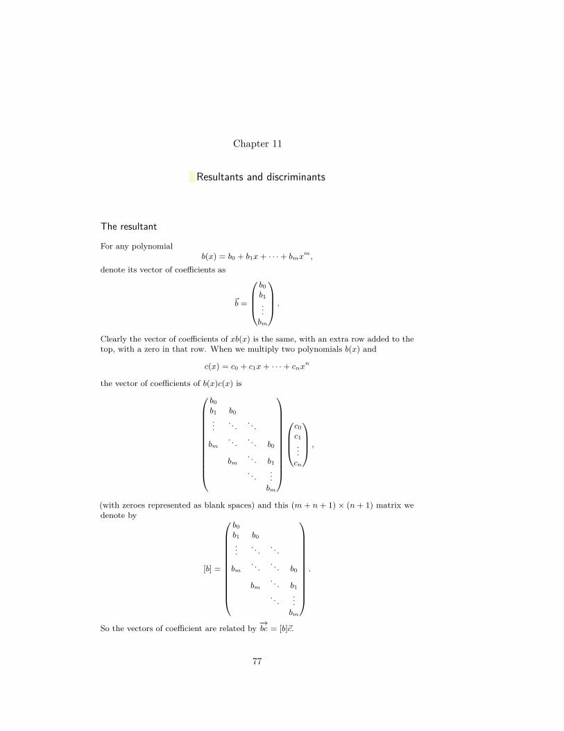
Chapter 11

Resultants and discriminants

The resultant

For any polynomialb(x) = b0 + b1x+ · · ·+ bmx

m,

denote its vector of coefficients as

~b =

b0b1...bm

.

Clearly the vector of coefficients of xb(x) is the same, with an extra row added to thetop, with a zero in that row. When we multiply two polynomials b(x) and

c(x) = c0 + c1x+ · · ·+ cnxn

the vector of coefficients of b(x)c(x) is

b0b1 b0...

. . . . . .

bm. . . . . . b0

bm. . . b1. . .

...bm

c0c1...cn

,

(with zeroes represented as blank spaces) and this (m+ n+ 1)× (n+ 1) matrix wedenote by

[b] =

b0b1 b0...

. . . . . .

bm. . . . . . b0

bm. . . b1. . .

...bm

.

So the vectors of coefficient are related by−→bc = [b]~c.

77

78 Resultants and discriminants

The resultant of two polynomials

b(x) = b0 + b1x+ · · ·+ bmxm and

c(x) = c0 + c1x+ · · ·+ cnxn,

denoted resb,c, is the determinant of the matrix([b] [c]

), given by stacking the

matrices [b] and [c] of suitable sizes beside one another, to get a square matrix of size(m+n)× (m+n). To remember the sizes: the number of columns in [b] is the degreeof c, while the number of columns in [c] is the degree of b.

If

b(x) = 4− x+ 7x2 + x3,

c(x) = −6 + 2x,

then resb,c is the determinant of the 4× 4 matrix 4 −6 0 0−1 2 −6 07 0 2 −61 0 0 2

,

which is resb,c = −712.

If we swap b and c, we swap columns, so clearly resc,b = (−1)mn resb,c.

Take b(x) = x2 + 4x+ 7 and c(x) = x3 and compute

resb,c = det

7 0 0 0 04 7 0 0 01 4 7 0 00 1 4 1 00 0 1 0 1

= 73.

The easiest examples of arbitrary degrees arise when we take any b(x) but try c(x) =xn:

resb,c = det

b0... b0...

. . . . . .

bm. . . . . . b0

bm. . .

... 1. . .

.... . .

bm 1

= bn0 .

Sage

Computing resultants in sage requires us to tell sage what sort of numbers arise asthe coefficients of our polynomials.

Common factors and resultants 79

P.<x> = PolynomialRing(QQ)a=x^3+x+7b=x^2+2a.resultant(b)

yields 51. The expression P.<x> = PolynomialRing(QQ) tells sage that we are workingwith polynomials with rational coefficients (QQ means rational) in a variable x.

We could write our own resultant function, just to see how it might work:

def resultant(b,c):B=b.list()C=c.list()m=len(B)-1n=len(C)-1A=matrix(m+n,m+n)for j in range(0,n):

for i in range(0,m+n):if (0<=i-j) and (i-j<=m):

A[i,j]=B[i-j]else:

A[i,j]=0for j in range(n,m+n):

for i in range(0,m+n):if (0<=i-j+n) and (i-j+n<=n):

A[i,j]=C[i-j+n]else:

A[i,j]=0return det(A)

Try it out:

t=var(’t’)p = t^2+2*t+1q = t+1resultant(p,q)

yields 0.

Common factors and resultants

Lemma 11.1. Two polynomials b(x) and c(x) of degrees m and n, over any field,have a nonconstant common factor just when

0 = u(x)b(x) + v(x)c(x)

for two polynomials u(x) and v(x) of degrees n− 1 and m− 1 at most, not both zero.

Proof. Two polynomials b(x) and c(x) of degreesm and n have a nonconstant commonfactor just when we can write the polynomials factored, say as b(x) = v(x)d(x) andc(x) = −u(x)d(x). But then

0 = u(x)b(x) + v(x)c(x).

80 Resultants and discriminants

On the other hand, suppose that

0 = u(x)b(x) + v(x)c(x)

for two polynomials u(x) and v(x) of degrees n− 1 and m− 1 at most. Suppose thatb(x) and c(x) have no common factor, so their greatest common divisor is 1. Writeout Bézout coefficients

1 = s(x)b(x) + t(x)c(x)and compute

v = vsb+ vtc,

= vsb+ tvc,

= vsb− tub,= b (vs− tu) .

But the degree of v is smaller than that of b, so v = 0. Swapping roles of b, c and ofu, v and of s, t, we get u = 0.

Proposition 11.2. Two polynomials, over any field, have a nonconstant commonfactor just when their resultant vanishes.

Proof. Take two polynomials

u(x) = u0 + u1x+ · · ·+ un−1xn−1,

v(x) = v0 + v1x+ · · ·+ vm−1xm−1.

The vector of coefficients of u(x)b(x) + v(x)c(x) is

−−−−→bu+ cv =

([b] [c]

)(~u~v

)By linear algebra, the determinant vanishes just when the matrix has a nonzero nullvector, i.e. a nonzero vector in its kernel. So the resultant vanishes just when thereis a choice of coefficients

u0, u1, . . . , v0, v1, . . . ,

not all zero, so that u(x)b(x) + v(x)c(x) = 0. In other words, there are polynomialsu(x) and v(x) of required degrees so that u(x)b(x) + v(x)c(x) = 0. The theorem nowfollows from lemma 11.1 on the previous page.

The resultant is brutal to compute, even for polynomials of fairly small degree.Its importance, like that of the determinant of a matrix, arises from its theoreticalpower.

11.1 Find the resultants, and use them to decide if there are nonconstant commonfactors.

a. x2 − 5x+ 6, x3 − 3x2 + x− 3b. x2 + 1, x− 1

11.2 Over the field of remainders modulo 2, calculate the resultant of b(x) = x3 +x2 + x+ 1, c(x) = x3 + x. Warning: the 6× 6 determinant you get is actually easierthan it looks at first, so look for tricks to find it without any hard calculation.

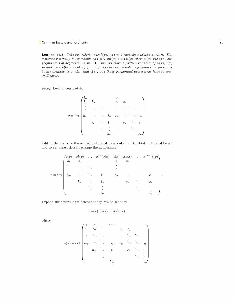
Common factors and resultants 81

Lemma 11.3. Take two polynomials b(x), c(x) in a variable x of degrees m,n. Theresultant r = resb,c is expressible as r = u(x)b(x) + v(x)c(x) where u(x) and v(x) arepolynomials of degrees n− 1,m− 1. One can make a particular choice of u(x), v(x)so that the coefficients of u(x) and of v(x) are expressible as polynomial expressionsin the coefficients of b(x) and c(x), and those polynomial expressions have integercoefficients.

Proof. Look at our matrix:

r = det

b0 c0b1 b0 c1 c0...

. . . . . ....

. . . . . .

bm. . . . . . b0 cn

. . . . . . c0

bm. . . b1 cn

. . . c1. . .

.... . .

...bm cn

Add to the first row the second multiplied by x and then the third multiplied by x2

and so on, which doesn’t change the determinant:

r = det

b(x) xb(x) . . . xn−1b(x) c(x) xc(x) . . . xm−1c(x)b1 b0 c1 c0...

. . . . . ....

. . . . . .

bm. . . . . . b0 cn

. . . . . . c0

bm. . . b1 cn

. . . c1. . .

.... . .

...bm cn

.

Expand the determinant across the top row to see that

r = u(x)b(x) + v(x)c(x)

where

u(x) = det

1 x . . . xn−1

b1 b0 c1 c0...

. . . . . ....

. . . . . .

bm. . . . . . b0 cn

. . . . . . c0

bm. . . b1 cn

. . . c1. . .

.... . .

...bm cn

82 Resultants and discriminants

and

v(x) = det

1 x . . . xm−1

b1 b0 c1 c0...

. . . . . ....

. . . . . .

bm. . . . . . b0 cn

. . . . . . c0

bm. . . b1 cn

. . . c1. . .

.... . .

...bm cn

Note that we can expand out any determinant using only multiplication and additionof entries and some ± signs.

If we scale up b(x) by a factor λ and look at the matrix whose determinant is ourresultant, we see that the resultant of b(x), c(x) scales by λn, where n is the degreeof c(x). So practically we only need to compute resultants of monic polynomials.

Proposition 11.4. Given two monic polynomials over any field, each factored intolinear factors,

b(x) = (x− β1) (x− β2) . . . (x− βm) ,c(x) = (x− γ1) (x− γ2) . . . (x− γn) ,

then the resultant is

resb,c = (β1 − γ1) (β1 − γ2) . . . (βm − γn) ,= c(β1) c(β2) . . . c(βm) ,= (−1)mnb(γ1) b(γ2) . . . b(γn) .

In particular, the resultant vanishes just when b(x) and c(x) have a common root.

Proof. We will only give the proof here for polynomials over an infinite field. We willgive the proof over finite fields in chapter 14. If we expand out the expression for b(x)into a sum of monomials, with coefficients being expressed in terms of these βi, andsimilarly for c(x), then the resultant is a huge polynomial expression in terms of thevarious βi and γj . This polynomial vanishes whenever βi = γj . Thinking of βi andγj as abstract variables, the expression βi − γj is a linear function. Assume for themoment that our field is infinite. Then the resultant is divisible by βi − γj , for any iand j, by lemma 10.7 on page 74. Therefore the resultant is divisible by

(β1 − γ1) (β1 − γ2) . . . (βm − γn) .

From our examples above, we see that the total number of such factors is mn, andtherefore each one arises just once, so our resultant is as described

resb,c = (β1 − γ1) (β1 − γ2) . . . (βm − γn) ,

except perhaps for a constant factor, which we check by looking at our examples. Fora finite field, we will fix up this proof in chapter 14; for the moment, the reader willhave to accept that this can be done somehow.

Common factors and resultants 83

If b(x) ..= x7 + 2x + 1 and c(x) ..= x − 1, then c(x) has root x = 1, and both aremonic, so

resb,c = (−1)7·1b(1) = (−1)(17 + 2 + 1) = −4.

11.3 Suppose that b(x) is monic and c(x) is not and that they both split into linearfactors. Prove that

resb,c = c(β1) c(β2) . . . c(βm) .

Lemma 11.5. For any polynomials b(x), c(x), d(x),

resb,cd = resb,c resb,d .

Proof. If all of the polynomials split into linear factors, the result is clear:

resb,cd = c(β1) d(β1) . . . c(βm) d(βm) ,= c(β1) c(β2) . . . c(βm) d(β1) d(β2) . . . d(βm) ,= resb,c resb,d .

We will see eventually (in theorem 15.2 on page 133) that, given any polynomialsb(x), c(x), d(x), we can always replace our field by a larger field in which all of thepolynomials b(x), c(x), d(x) split into linear factors.

11.4 Suppose that b(x) is a monic polynomial which splits into linear factors. Provethat

resb,c+db = resb,cfor any polynomials c(x) and d(x). A surprise: note that the degree of c(x) +d(x)b(x)could be either that of c(x) or that of d(x)b(x), or something smaller than either, asany number of terms in c(x) + d(x)b(x) might cancel one another. But surprisingly,we don’t need to know the degree of c(x) + d(x)b(x).

11.5 A fast trick to find resultants: use the result of the previous problem to computeresb,c where

b(x) = x8 + 4x2 + 2x+ 1,c(x) = x6 + 4.

We can make sage code for our fast trick:

R.<x> = PolynomialRing(QQ)def fastresultant(b,c):

m=b.degree()n=c.degree()if m<n:

return (-1)^(m*n)*fastresultant(c,b)if n==0:

if m==0:return 1

return c(0)^mlb=b.leading_coefficient()lc=c.leading_coefficient()B=b/lb

84 Resultants and discriminants

C=c/lcr=B % Cif (r==0):

return 0return (-1)^(m*n)*lb^n*lc^m*fastresultant(C,r)

so that fastresultant(x^3+x+7,x^2+2) yields 51.

The discriminant

For any polynomial p(x), with any sort of coefficients, say

p(x) = a0 + a1x+ · · ·+ anxn,

we define the derivative

p′(x) = a1 + 2a2x+ 3a3x2 + · · ·+ nanx

n,

just imitating calculus. There is no interpretation of this as a “rate of change”, sincethe coefficients could be remainders modulo some integer, or something much stranger.

The discriminant ∆p of a polynomial p(x) is the resultant with the derivative:∆p

..= resp,p′ . By definition, the discriminant vanishes just when the polynomial hasa common factor with its derivative. For example, over the complex numbers, thediscriminant vanishes just when the polynomial has a “multiple root”, i.e. a repeatedlinear factor:

p(z) = (z − z0)2 . . . .

11.6 Find the discriminants of (a) ax2 + b + c, (b) x3 + x2, (c) x3 + x2 + 1, (d)x3 + 2x− 1 and explain what they tell you about these polynomials.

The polynomial f(x) = 1 + 2x2 + x4 over the real numbers has no real roots. Itsderivative is f ′(x) = 4x+ 4x3, so its discriminant is

∆f = det

1 0 0 0 0 0 00 1 0 4 0 0 02 0 1 0 4 0 00 2 0 4 0 4 01 0 2 0 4 0 40 1 0 0 0 4 00 0 1 0 0 0 4

= 0

(after a long calculation). So f(x) has a common factor with f ′(x). We can see thecommon factor more clearly if we factor:

f(x) = 1 + 2x2 + x4 =(1 + x2)2 ,

f ′(x) = 4x+ 4x3 = 4x(1 + x2) .

So f(x), f ′(x) share a common factor of 1 + x2. They don’t share a root over thereal numbers, but over the complex numbers

f(x) = (x− i)2 (x+ i)2 ,

f ′(x) = 4x(x− i)(x+ i),

so they share roots at x = ±i, the double roots of f(x).

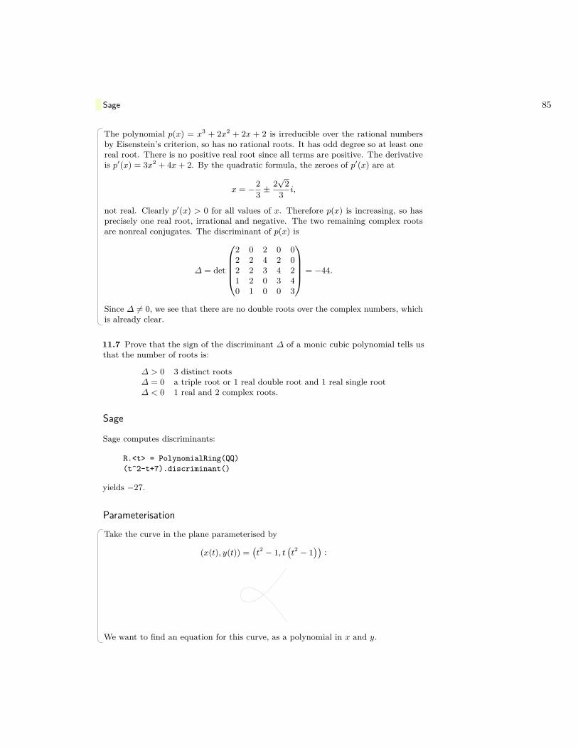
Sage 85

The polynomial p(x) = x3 + 2x2 + 2x + 2 is irreducible over the rational numbersby Eisenstein’s criterion, so has no rational roots. It has odd degree so at least onereal root. There is no positive real root since all terms are positive. The derivativeis p′(x) = 3x2 + 4x+ 2. By the quadratic formula, the zeroes of p′(x) are at

x = −23 ±

2√

23 i,

not real. Clearly p′(x) > 0 for all values of x. Therefore p(x) is increasing, so hasprecisely one real root, irrational and negative. The two remaining complex rootsare nonreal conjugates. The discriminant of p(x) is

∆ = det

2 0 2 0 02 2 4 2 02 2 3 4 21 2 0 3 40 1 0 0 3

= −44.

Since ∆ 6= 0, we see that there are no double roots over the complex numbers, whichis already clear.

11.7 Prove that the sign of the discriminant ∆ of a monic cubic polynomial tells usthat the number of roots is:

∆ > 0 3 distinct roots∆ = 0 a triple root or 1 real double root and 1 real single root∆ < 0 1 real and 2 complex roots.

Sage

Sage computes discriminants:

R.<t> = PolynomialRing(QQ)(t^2-t+7).discriminant()

yields −27.

Parameterisation

Take the curve in the plane parameterised by

(x(t), y(t)) =(t2 − 1, t

(t2 − 1

)):

We want to find an equation for this curve, as a polynomial in x and y.

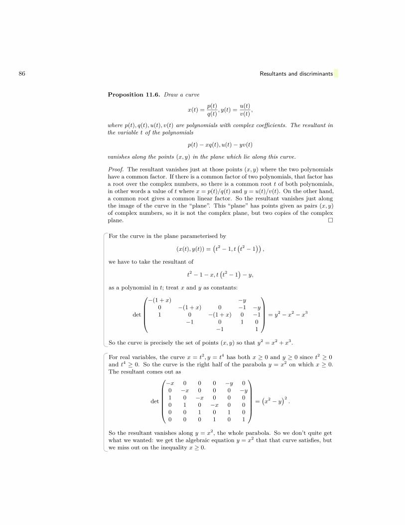
86 Resultants and discriminants

Proposition 11.6. Draw a curve

x(t) = p(t)q(t) , y(t) = u(t)

v(t) ,

where p(t), q(t), u(t), v(t) are polynomials with complex coefficients. The resultant inthe variable t of the polynomials

p(t)− xq(t), u(t)− yv(t)

vanishes along the points (x, y) in the plane which lie along this curve.

Proof. The resultant vanishes just at those points (x, y) where the two polynomialshave a common factor. If there is a common factor of two polynomials, that factor hasa root over the complex numbers, so there is a common root t of both polynomials,in other words a value of t where x = p(t)/q(t) and y = u(t)/v(t). On the other hand,a common root gives a common linear factor. So the resultant vanishes just alongthe image of the curve in the “plane”. This “plane” has points given as pairs (x, y)of complex numbers, so it is not the complex plane, but two copies of the complexplane.

For the curve in the plane parameterised by

(x(t), y(t)) =(t2 − 1, t

(t2 − 1

)),

we have to take the resultant of

t2 − 1− x, t(t2 − 1

)− y,

as a polynomial in t; treat x and y as constants:

det

−(1 + x) −y

0 −(1 + x) 0 −1 −y1 0 −(1 + x) 0 −1

−1 0 1 0−1 1

= y2 − x2 − x3

So the curve is precisely the set of points (x, y) so that y2 = x2 + x3.

For real variables, the curve x = t2, y = t4 has both x ≥ 0 and y ≥ 0 since t2 ≥ 0and t4 ≥ 0. So the curve is the right half of the parabola y = x2 on which x ≥ 0.The resultant comes out as

det

−x 0 0 0 −y 00 −x 0 0 0 −y1 0 −x 0 0 00 1 0 −x 0 00 0 1 0 1 00 0 0 1 0 1

=(x2 − y

)2.

So the resultant vanishes along y = x2, the whole parabola. So we don’t quite getwhat we wanted: we get the algebraic equation y = x2 that that curve satisfies, butwe miss out on the inequality x ≥ 0.

Sage 87

11.8 Find a nonconstant polynomial equation f(x, y) = 0 satisfied by the points ofthe curve

x(t) = t2, y(t) = t3 − t.

11.9 Find a nonconstant polynomial equation f(x, y) = 0 satisfied by the points ofthe curve

x(t) = t2 + t, y(t) = 1t.

11.10 Find a nonconstant polynomial equation f(x, y) = 0 satisfied by the points ofthe curve

x(t) = t2 + 1, y(t) = t+ 1t.

Sage

Sage handles 2 variable polynomials:

P.<x,y> = PolynomialRing(QQ)a = x + yb = x^3 - y^3a.resultant(b)

yields −2y3. If we want to use the resultant in the other variable, we specify whichvariable to get rid of: a.resultant(b, y) yields 2x3. Sage will take a parameterisationof a curve and give us the equation of the curve. Our example above becomes:

R.<x,y,t> = PolynomialRing(QQ)(t^2-1-x).resultant(t*(t^2-1)-y,t)

yields −x3 − x2 + y2.

Chapter 12

Groups

Numbers measure quantity, groups measure symmetry

— Mark ArmstrongGroups and Symmetry

The theory of groups is, as it were, the whole of mathematics strippedof its matter and reduced to pure form.

— Henri Poincaré

Transformation groups

Take a set X, which could be a set of points in the plane, or a set of numbers, or acollection of various geometric figures, or the set of books in a library, or any otherset of any sort of things. A transformation f of X associates to each element x of Xsome element f(x) also from X.

Take a square X in the plane, and rotate it around its centre by a right angle. Eachpoint p of X is rotated into some point f(p). Note that the centre point of the squareis “fixed”, i.e. rotated into itself.

Take any set X. The identity transformation is the transformation that leaves everypoint of X where it is: f(x) = x.

Shuffle a deck of cards. If X is the set of cards, the shuffle is a transformation f ofX.

Two maps f : X → Y and g : Y → X between sets are inverses if f(g(x)) = xand g(f(x)) = x for any element x of X. In other words, f ◦ g and g ◦ f are both theidentity transformation. Recall that a map f is invertible, also called a bijection or apermutation if it has an inverse. A bijection transformation is a permutation.

12.1 A map f : X → Y of a set X is injective (also called one-to-one) if f(p) = f(q)only when p = q. It is surjective (also called onto) if every element y of Y has theform y = f(x) for some element x of X. Prove that a map is a bijection just when itis injective and surjective.

89

90 Groups

12.2 Prove that a transformation f of a finite set X is injective just when it issurjective, and hence just when it is a bijection.

12.3 Prove that a bijection f has a unique inverse.

The inverse of a bijection f is denoted f−1.A transformation group G on a set X is a nonempty collection of permutations of

X so thata. if f and g are in G then f ◦ g is in G.b. if f is in G then f−1 is also in G.

Take X the Euclidean plane. Every rotation of the plane around the origin is bysome angle, say θ. Conversely, every angle θ is the angle of some rotation around theorigin. So angles form a transformation group G, the group of rotations of the planeX around the origin.

Take X to be three dimensional Euclidean space. Take a line ` through the origin,with a chosen direction along that line. Hold the line in your hand, so that yourthumb points up the chosen direction. Then your figures curl around the line ina certain direction. In additional, take an angle θ, and rotate the whole space Xaround in the direction of your fingers, by the angle θ. Every rotation of Euclideanspace X arises in this way. (If you change the choice of direction to point your thumb,but keep the same axis of rotation `, then you change θ to −θ.) When you composea rotation with another rotation, the result is yet a third rotation. The rotations ofEuclidean space form a transformation group G.

Take X to be the real number line. Given any real number t, we can define atransformation f(x) = x + t. In this way, the real numbers t are associated to theelements of a group G of transformations of the real number line.

A rigid motion of Euclidean space is a transformation that preserves distances. Forexample, rotations, mirror reflections: (x, y) 7→ (x,−y), and translations (x, y) 7→(x+x0, y+y0) are rigid motions of the plane. The rigid motions form a transformationgroup.

Take a geometric figure X in the plane, or in space. A rigid motion preserving X isa symmetry of X; the symmetries of a figure constitute a transformation group. Forexample, if X is a square, every symmetry permutes the corners somehow, and wecan easily see these symmetries:

1

2 3

4 4

1 2

3 1

4 3

2

The symmetry group of a non-isosceles triangle consists just of the identity transfor-mation. For an isosceles, but not equilateral, triangle, the symmetry group is theidentity transformation and the reflection across the axis of symmetry. An equilateraltriangle has as symmetries: the identity transformation, the rotation by 120◦, therotation by 240◦, and the three reflections in the three axes of symmetry.

12.4 Consider a brick, i.e. a rectangular box whose length, width and height are allunequal. What is its symmetry group?

Transformation groups 91

The symmetry group of an infinitely repeating sodium choride lattice

includes the translations of space that move each green chlorine atom and purplenatrium atom to its neighbor, up, down, left, right, forward or back, and mirrorreflections around the coordinate planes through the origin, where we put the originin the middle of any one of these atoms, and also the transformations given bypermuting the order of the variables x, y, z of each coordinate axis.

Every 2× 2 matrix

A =(a bc d

)(with entries from any chosen field) determines a linear transformation:(

xy

)7→ A

(xy

)=(a bc d

)(xy

)=(ax+ bycx+ dy

)of the plane. Similarly, a square matrix A, say n × n, determines a linear trans-formation of n-dimensional Euclidean space. A linear transformation is a bijectionjust when the associated matrix A is invertible, i.e. just when A has nonzero de-terminant. The invertible n × n matrices form a transformation group G, of lineartransformations of n-dimensional Euclidean space.

Take X to be the set of numbers { 1, 2, 3, 4 }. The symmetric group on 4 letters is thegroup G of all permutations of X. The terminology “on 4 letters” reminds us thatwe could just as well have taken X = { a, b, c, d } to consist of any 4 distinct elements,and then we would get essentially the same story, just relabelling. It is convenientnotation to write a permutation of finite sets as, for example,(

1 2 3 42 3 1 4

)to mean the map f so that f(1) = 2, f(2) = 3, f(3) = 1 and f(4) = 4, i.e. readingdown from the top row as the input to f to the entry underneath as the output of f .It is often understood that the first row is just 1 2 3 4 or some such, so we can justwrite down the second row: 2 3 1 4, to display the permutation.

12.5 What is are the permutations g ◦ f and f ◦ g where g is 2 3 1 4 and f is 3 1 2 4?

12.6 A regular tetrahedron is a pyramid with triangular base, all of whose sides areequilateral triangles. Prove that the symmetry group of the regular tetrahedron isthe symmetric group on 4 letters.

92 Groups

Another notation for permutations: the cycle (1342) means the permutation thattakes 1 to 3, 3 to 4, 4 to 2 and 2 to 1, reading from left to right. More generally,the cycle (a1a2 . . . ak) is the permutation taking a1 to a2, a2 to a3, and so on, andtaking ak to a1. So (2314) takes 3 to 1. By definition, if we have a number x which isnot among these various a1, a2, . . . , ak, then the cycle (a1a2 . . . ak) fixes the numberx: (2354) takes 1 to 1. Two cycles (a1a2 . . . ak) and (b1b2 . . . b`) are disjoint if noneof the ai occur among the bj and vice versa. So

(1452) is disjoint from (36),

but(1352) is not disjoint from (36)

since they both have 3 in them. We can write the identity permutation as (). Notethat any cycle of length 1 is also the identity transformation: (2) = (1) = (), since (2)takes 2 to 2, and fixes everything else. If two permutations f and g can be expressedas disjoint cycles, then fg = gf , since each fixes all of the letters moved by the other.

Sage knows how to multiply cycles:

G = SymmetricGroup(5)sigma = G("(1,3) (2,5,4)")rho = G([(2,4), (1,5)])rho^(-1) * sigma * rho

prints (1, 2, 4)(3, 5).

Theorem 12.1. Every permutation of the elements of a finite set is expressed as aproduct of disjoint cycles, uniquely except for the order in which we write down thecycles, which can be arbitrary.

Proof. Suppose our finite set is 1, 2, . . . , n. Our permutation f takes 1 to some numberf(1), takes that number to some other number f(f(1)), and so on, and eventually(because there are finitely many), if we repeat it enough times we cycle back to anumber we have seen before. Suppose that this first happens at the k-th step. Writingf21 to mean f ◦f(1), not multiplication but composition, we are saying that fk1 mustalready be among 1, f1, . . . , fk−11, say fk1 = f `1 for some 0 ≤ ` < k. Suppose thatwe pick k the smallest possible Since f is a bijection, if ` > 0 we apply f−1 to bothsides of fk1 = f `1 to find a smaller value of k, a contradiction. So ` = 0, i.e. fk1 = 1is our first repeat. So we have a cycle (1 f1 . . . fk−11). But that cycle might notexhaust the whole of f , since there might be some other numbers among 1, 2, . . . , nnot among the elements of this cycle.

Take the smallest one, say b. Since f is a bijection, if any number from b, fb, f2b, . . .is also in the cycle (1 f1 f21 . . . fk−11, we can apply f−1 to both sides as manytimes as we need to get that b is already in that cycle, a contradiction. By the sameargument above, replacing 1 by b, we get another cycle (b fb . . . f `−1b) disjoint fromthe first. Continue in this way by induction to express f as a product of disjointcycles. This expression is unique, since each cycle is precisely built from applyingf repeatedly to any element until a cycle forms, so any two such expressions haveexactly the same cycle through any element.

For example, in cycle notation(1 2 3 42 3 1 4

)= (123)

Transformation groups 93

and (1 2 3 4 53 4 1 5 2

)= (13)(245).

12.7 Prove that any set with n elements has n! permutations, in several ways: bycounting

a. how many places to move 1 to, and then how many places there are left to move2 to, and so on,

b. the number of places to stick object n in between the elements of any givenpermutation a1a2 . . . an−1 of the numbers 1, 2, . . . , n−1, say as na1a2 . . . an−1 ora1na2 . . . an−1 or a1a2n . . . an−1 and so on, for example: given the permutation

3 1 2

of the numbers 1, 2, 3, we can put 4 in there as

4 3 1 2, 3 4 1 2, 3 1 4 2, or 3 1 2 4.

c. the number of ways to put at the end of a given permutation a1a2 . . . an−1 somenumber b from among

b = 12 , 1 + 1

2 , . . . , n−12 ,

for example into the permutation 3 1 2 we stick

3 1 2 12 , or 3 1 2 3

2 , or 3 1 2 52 , or 3 1 2 7

2

and then replace the numbers in the list by integers from 1, 2, . . . , n, but in thesame order:

4 2 3 1, or 4 1 3 2, or 4 1 2 3, or 3 1 2 4.

d. the possible disjoint cycles.

12.8 Prove that there is an element g of the symmetric group on 7 letters so that(147)(23) and (235)(14) are conjugate, i.e. (235)(14) = g(147)(23)g−1. More generally,prove that two elements of the symmetric group on n letters are conjugate just when,when we write them as products of disjoint cycles, the numbers of cycles of each lengthare the same.

Sage knows all of the permutations of small symmetric groups, and will print themout for you in cycle notation:

H = DihedralGroup(6)H.list()

yields, (1, 6)(2, 5)(3, 4), (1, 2, 3, 4, 5, 6),(1, 5)(2, 4), (2, 6)(3, 5), (1, 3, 5)(2, 4, 6),(1, 4)(2, 3)(5, 6), (1, 6, 5, 4, 3, 2), (1, 4)(2, 5)(3, 6),(1, 2)(3, 6)(4, 5), (1, 5, 3)(2, 6, 4), (1, 3)(4, 6)

where the identity element is the blank space at the start.

94 Groups

Groups

Each symmetry of an equilateral triangle in the plane permutes the vertices. If welabel the vertices, say as 1, 2, 3, then every permutation of the labels 1, 2, 3 occursfrom a unique symmetry of the triangle. So the symmetries of the equilateral trianglecorrespond to the permutations of the labels, i.e. the symmetry group of the equilateraltriangle is, in some sense, the same as the symmetric group on three letters. It isthis notion of correspondence that leads us to see that two transformation groupscan be “the same” while they are transforming very different sets; in our example,the symmetries of the equilateral triangle transform the infinitely many points of thetriangle, while the permutations of three letters transform a set of three letters. Inorder to say what is “the same” in the two transformation groups, we need a moreabstract concept of group.

A group is a set G so thata. To any elements a, b of G there is associated an element ab of G, called the

product of a and b.b. The product is associative: if a, b, c are elements of G, then (ab)c = a(bc), so

that either expression is denoted as abc.c. There is an identity element: some element 1 of G, so that a1 = 1a = a for any

element a of G.d. Every element is invertible: if a is an element of G, there is an element, denoted

a−1, of G for which aa−1 = a−1a = 1.

Nonzero rational numbers form a group G under usual multiplication, where a−1

means the reciprocal of any rational number a. Note that 0 does not have a reciprocal,so we have to remove it.

Nonzero elements of any field form a group G under usual multiplication, where a−1

means the reciprocal of any element a. Note that 0 does not have a reciprocal, so wehave to remove it.

Any transformation group G is a group, using composition of transformations as itsproduct, and the identity transformation as its identity element. In particular, asexamples of groups: the symmetry groups of geometric figures, the group of invertiblematrices (under matrix multiplication), the symmetry group on some letters, thegroup of rotations of the Euclidean plane, and the group of rotations of Euclideanspace.

It is easier to check if a collection of transformations forms a transformation groupthan to check if some abstract product operation forms a group; almost all of ourexamples of groups will be transformation groups in some obvious way.

Two elements a, b of a group commute if ab = ba. A group is abelian if any twoelements of the group commute.

Nonzero rational numbers form an abelian group under usual multiplication.

Nonzero elements of any field form an abelian group under usual multiplication.

Invertible 2 × 2 matrices, with entries drawn from some chosen field, form an non-abelian group under usual matrix multiplication.

Additive notation 95

The symmetries of the equilateral triangle form a non-abelian group: if we rotate by120◦ and the reflect across an angle bisector, we get a different result than if we firstreflect across that bisector and then rotate.

12.9 Prove that, for any elements a, b, c, d of a group G,

a(b(cd)) = (ab)(cd) = ((ab)c)d.

Generalize by induction to prove that parentheses are not needed in expressions ofany length.

12.10 For any element a of a group G, define a0 to mean 1, and define by inductionan+1 = aan. Prove by induction that aman = am+n for an integers m,n.

12.11 Suppose that 1, 1′ are two elements of a group G, and that a1 = 1a = a andalso that a1′ = 1′a = a for any element a of the group G). Prove that 1 = 1′.

12.12 Given elements a, b of a group G, prove that the equation ax = b has a uniquesolution x in G. Prove also that the equation ya = b has a unique solution y in G.

12.13 Prove that (ab)−1 = b−1a−1 for any elements a, b of any group.

12.14 Suppose that x belongs to a group G and that x2 = x. Prove that x = 1.

12.15 Prove that the set of nonzero rational numbers, with product operation definedas usual division, do not form a group. (It might help to write the operation is somefunny notation like a?b, instead of ab, which easily gets confused with multiplication.)

Additive notation

When a group is abelian, it is often preferred to write the group operation not as abbut instead as a+ b, and the identity element as 0 rather than 1, and the inverse as−a rather than a−1.The set of integers form an abelian group, where the group operation is usual addition.

Any field is an abelian group, where the group operation is usual addition.

The set of 2 × 2 matrices, with integer entries form an abelian group, where thegroup operation is usual addition. The same for rational entries, real entries, complexentries, entries drawn from any field, and for 2× 3 matrices, and so on.

The rotations of the plane around the origin form an abelian group, writing each rota-tion in terms of its angle of rotation, and using addition of angles, i.e. composition ofrotations, as the group operation. (Careful: the rotations of Euclidean 3-dimensionalspace form a non-abelian group.)

12.16 Define an operation on real numbers b, c by

b ? c = b+ c

1− bc .

With this operation, are the real numbers an abelian group? Consider the collectionconsisting of all numbers of the form b = 3p

qwith p, q integers so that 3 does not

divide q. Is this collection of numbers a group under this operation?

96 Groups

12.17∗ Suppose that we turn the real numbers R into a group using some weirdmultiplication, say x ∗ y = p(x, y) and with some identity element x0. Suppose thatp(x, y) is a polynomial. Prove that p(x, y) is given by the formula p(x+ x0, y+ x0) =x+ y + x0.

Sage knows many finite groups, and can say whether they are abelian:

H = SymmetricGroup(6)H.is_abelian()

yields False.

Multiplication tables

If a group G is finite (i.e. has finitely many elements), we let |G| be the numberof elements of G, called the order of G. We can then write a multiplication table,with rows representing some element x, columns some element y, and entries xy Forexample, if a group G has 2 elements, say 1 and a, then it is easy to see that a2 = 1so the multiplication table must be

1 a

1 1 aa a 1

12.18 Prove that, for any group, on every row of its multiplication table, everyelement of the group occurs exactly once. Prove the same for columns instead of rows.

12.19 Prove that any group G of order 3 has (in some labelled of its elements) themultiplication table

1 a b

1 1 a ba a b 1b b 1 a

If G and H are two groups, their product is the group G×H whose elements arepairs (g, h) of elements g of G and h of H, with product

(g1, h1)(g2, h2) = (g1g2, h1h2)

and identity element (1, 1). Given a multiplication table for G and one for H, we canmake one for G×H by taking each row a and column b entry ab for G, and each rowx and column y entry xy for H, and writing out (a, x) as a row for G×H, (b, y) as arow for G×H, and (ab, xy) as entry. For example, if G = H are both the group oforder 2 above, then G×H has multiplication table:

1 (a, 1) (1, a) (a, a)1 1 (a, 1) (1, a) (a, a)

(a, 1) (a, 1) 1 (a, a) (1, a)(1, a) (1, a) (a, a) 1 (a, 1)(a, a) (a, a) (1, a) (a, 1) 1

An isomorphism φ : G→ H is a bijection between elements of two groups G andH so that φ(xy) = φ(x)φ(y): φ preserves multiplication. If there is some isomorphismbetween two groups, they are isomorphic, and for all purposes of algebra we can treatthem as being the same group.

Multiplication tables 97

In problem 12.19 on the facing page, we saw that all groups of order 3 are isomorphic.

The remainders modulo 4 form a group G1, under addition as the group operation.The set of complex numbers G2 = { 1,−1, i,−i } form a group under multiplication.

The matrices (1 00 1

),

(0 1−1 0

),

(−1 00 −1

),

(0 −11 0

)form a group G3 under multiplication. All of these groups are isomorphic. Forexample, map 0 7→ 1, 1 7→ i, 2 7→ −1, 3 7→ −i to map G1 → G2.

Let G be the group of order 2 we found above and H the group of remainders modulo4. The groups G × G and H are both of order 4, but they are not isomorphic,because H contains the element 1 and every element of H is expressed in terms of 1as precisely one of the 4 elements

1, 1 + 1, 1 + 1 + 1, 1 + 1 + 1 + 1.

So if G (in multiplication notation!) were isomorphic to H, we would have to findsome element (x, y) of G so that the 4 elements

(x, y), (x, y)2, (x, y)3, (x, y)4

constitute the whole of G. Check the multiplication table above to see that every(x, y) in G satisfies (x, y)2 = (1, 1).

12.20 How many groups of order four are there, up to isomorphism?

Sage knows the multiplication tables of many groups. The dihedral group Dn isthe symmetry group of a regular polygon with n equal sides and angles. If we type

H = DihedralGroup(6)H.cayley_table()

we see the multiplication table:

· a b c d e f g h i j k l

a a b c d e f g h i j k lb b a e h c j k d l f g ic c d f g b i l a k e h jd d c b a f e h g j i l ke e h j k a l i b g c d ff f g i l d k j c h b a eg g f d c i b a l e k j hh h e a b j c d k f l i gi i l k j g h e f a d c bj j k l i h g f e d a b ck k j h e l a b i c g f dl l i g f k d c j b h e a

where a is the identity element.

98 Groups

Cyclic groups

A group G is cyclic if it consists of the powers of a single element x, i.e. G consistsof the powers xn for integers n. For example, the integers (written additively) aregenerated by multiplies of 1, as is the group of remainders modulo some integer n ≥ 0.

Theorem 12.2. Every cyclic group G is isomorphic to either the integers (when|G| =∞) or to the integers modulo an integer n ≥ 0, when |G| = n.

Proof. Suppose that G consists of the powers xk of a single element x. Define a mapf : Z → G by f(k) = xk. Then clearly f(k + `) = xk+` = xkx` = f(k)f(`). If fis a bijection, then f is our isomorphism. So suppose that f is not a bijection. Bydefinition, f is surjective, so f must fail to be injective, i.e. f(k) = f(`) for somek 6= `, i.e. xk = x`, i.e. xk−` = 0 i.e. f(k − `) = 1. Let K ⊂ Z be the set of allintegers m so that f(m) = 1. Note that K contains zero, and K also contains somenonzero element k − `. If m is in K then xm = 1 so x2m = 1 and so on, i.e. if m isin K then all multiples of m are in K. If K contains some integers b, c, take Bézoutcoefficients sb+ tc = g and then

f(g) = f(sb+ tc) = xsb+tc = (xb)s(xc)t = 1s1t = 1.

Hence g is in K as well: the greatest common divisor n of all elements of K alsolies in K. But then every multiple of n also lies in K. Hence K consists preciselyof all multiples of n, i.e. K = nZ, and so G = { 1, x, . . . , xn−1 } is isomorphic to theremainders modulo n, taking each remainder b to xb.

The order of an element a of a group G is the order of the cyclic group consistingof the powers ak.

12.21 Take any two elements a, b of some group. Prove that ab and ba have the sameorder.

12.22 Take any two elements a, b of order two in some group. If ab also has ordertwo, prove that a and b commute.

12.23 Take a permutation f of n letters 1, 2, . . . , n, expressed as a product of disjointcycles. Prove that the order of f is the least common multiple of the orders of thedisjoint cycles.

Sage can compute the order of an element of a group:

G = SymmetricGroup(5)sigma = G("(1,3) (2,5,4)")sigma.order()

yields 6.

Graphs

Take a hexagon X in the plane and let G be its symmetry group. Label the verticesof X in order as we travel around the vertices counterclockwise, say as 1, 2, 3, 4, 5, 6.

Graphs 99

12

3

4 5

6

Any symmetry moves 1 to one of the six vertices, and moves 2 to a next door neighborvertex. We can draw the vertices of the hexagon twice, one for drawing where 1 istaken to, and once again to represent whether 2 is taken to the vertex counterclockwisefrom 1 or clockwise.

In a sense, this is a picture of the group, since every element of the group is completelydetermined once we know where vertices 1 and 2 go: the rest are then in ordercyclically around the hexagon. Let b be rotation of the hexagon by 60◦, and let c bereflection of the hexagon across the axis of symmetry through vertex 1. Label theelements of the group according to how they move vertices 1 and 2, i.e. how muchof b and c they contain:

b1c

b1

b2c

b2

b3cb3

b4c

b4

b5c

b5

c 1

Multiplication of each element by b on the left, i.e. x 7→ bx, spins the hexagon aroundto right.

100 Groups

b1c

b1

b2c

b2

b3cb3

b4c

b4

b5c

b5

c 1

Multiplication of each element by c on the right, i.e. x 7→ xc, moves the inwardhexagon points to the outward ones, and vice versa.

Elements g, h, . . . of a group G generate that group if every element can be writtenas a product of integer powers of those elements. If we fix some elements generatinga group G, the Cayley graph of G (with respect to those generators) is the set ofelements of G, each draw as a dot, together with an arrow from one dot to another,labelled by g, if the first dot is some element k and the second is gk (or kg, dependingon which ordering we prefer). These pictures are almost never useful in proving resultsabout groups, but they give us some intuition.

Sage knows the Cayley graphs (for various generators) of many groups. If we type

H = DihedralGroup(6)show(H.cayley_graph())

we see the graph:

The graph is labelled by the cycles of each element, thought of as a permutation ofthe vertices of the hexagon.

Subgroups

A subset H of a group G is a subgroup if

Cosets 101

a. H contains the identity element andb. if a and b are elements of H then ab is also an element of H,c. if b is an element of H then b−1 is also an element of H.It follows that H is itself a group.

The even numbers are a subgroup of the integers, under usual integer addition.

The invertible integer 2 × 2 matrices are a subgroup of the invertible real 2 × 2matrices.

If b is an element of any group G, then the set of all elements of G of the form bk forintegers k is a cyclic group, the subgroup generated by b.

The real 2 × 2 matrices of unit determinant form a subgroup of the group of allinvertible real 2× 2 matrices, since determinants multiply.

12.24 What are all of the subgroups of the symmetry group of a hexagon?

Cosets

If S is any subset of a group G and b is any element of G, denote by bS the set ofelements of the form bs for s in S, called a left translate or left coset of S; if we writecoset, we mean left coset. Denote by Sb the set of elements of the form sb for s inS, called a right translate or right coset of S. Each coset bS has the same number ofelements as S, since s 7→ bs has inverse t 7→ b−1t, so is a bijection.

The group G of symmetries of the hexagon has a subgroup H of rotations of thehexagon. Divide up G into H-cosets:

b1c

b1

b2c

b2

b3cb3

b4c

b4

b5c

b5

c 1

We might draw our cosets as columns of a matrix

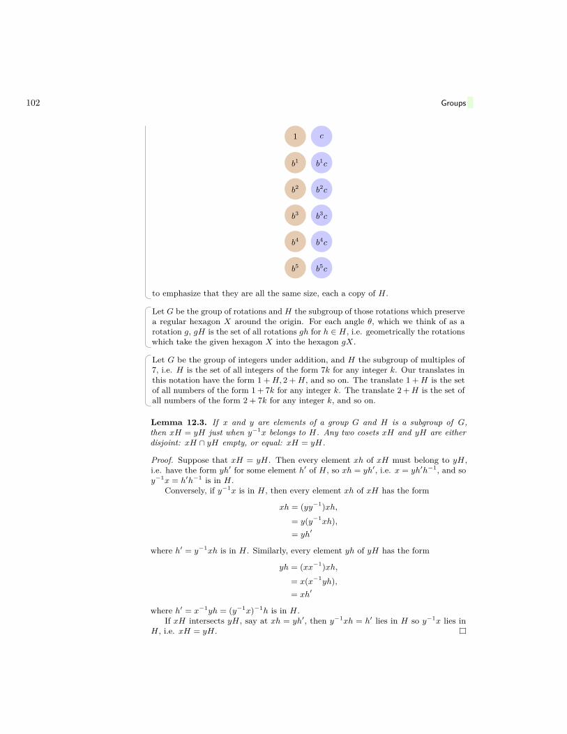
102 Groups

b1cb1

b2cb2

b3cb3

b4cb4

b5cb5

c1

to emphasize that they are all the same size, each a copy of H.

Let G be the group of rotations and H the subgroup of those rotations which preservea regular hexagon X around the origin. For each angle θ, which we think of as arotation g, gH is the set of all rotations gh for h ∈ H, i.e. geometrically the rotationswhich take the given hexagon X into the hexagon gX.

Let G be the group of integers under addition, and H the subgroup of multiples of7, i.e. H is the set of all integers of the form 7k for any integer k. Our translates inthis notation have the form 1 +H, 2 +H, and so on. The translate 1 +H is the setof all numbers of the form 1 + 7k for any integer k. The translate 2 +H is the set ofall numbers of the form 2 + 7k for any integer k, and so on.

Lemma 12.3. If x and y are elements of a group G and H is a subgroup of G,then xH = yH just when y−1x belongs to H. Any two cosets xH and yH are eitherdisjoint: xH ∩ yH empty, or equal: xH = yH.

Proof. Suppose that xH = yH. Then every element xh of xH must belong to yH,i.e. have the form yh′ for some element h′ of H, so xh = yh′, i.e. x = yh′h−1, and soy−1x = h′h−1 is in H.

Conversely, if y−1x is in H, then every element xh of xH has the form

xh = (yy−1)xh,= y(y−1xh),= yh′

where h′ = y−1xh is in H. Similarly, every element yh of yH has the form

yh = (xx−1)xh,= x(x−1yh),= xh′

where h′ = x−1yh = (y−1x)−1h is in H.If xH intersects yH, say at xh = yh′, then y−1xh = h′ lies in H so y−1x lies in

H, i.e. xH = yH.

Actions 103

If H is a subgroup of a group G, we let G/H be the collection of all cosets of Hin G.

The group G of symmetries of the hexagon has a subgroup H of rotations of thehexagon. If we draw each coset as a column, we draw each point of G/H as a singledot underneath that column:

b1cb1

b2cb2

b3cb3

b4cb4

b5cb5

c1

cH1H

Let G be the group of all rotations of the plane and H the subgroup of those rotationswhich preserve a regular hexagon X around the origin. For each angle θ, which wethink of as a rotation g, gH is the set of all rotations gh for h ∈ H, i.e. geometricallythe rotations which take the given hexagon X into the hexagon gX. So each cosetgH in G/H is identified with a rotated hexagon gX, i.e. G/H is the set of all rotatedhexagons gX for any rotation g.

Let G be the group of integers under addition, and H the subgroup of multiples of 7,i.e. H is the set of all integers of the form 7k for any integer k. Our translates in thisnotation have the form 1 +H, 2 +H, and so on. The translate 1 +H is the set of allnumbers of the form 1 + 7k for any integer k, which we denote by 1. The translate2 +H is the set of all numbers of the form 2 + 7k for any integer k, which we denoteby 2, and so on. Of course, 7 = 0 is the coset of H. So G/H is the set of remaindersmodulo 7. Each element of G/H represents “gluing together” all elements of G thatdiffer by a multiple of H.

Actions

A group G acts on a set X if each element b of G has an associated transformationfg of X so that fbc = fb ◦ fc for any elements b, c of G. So then G is a transformationgroup of X, and write gx to mean fg(x). The action is transitive if any two pointsp, q of X are connected by some element of G, i.e. q = gp for some g in G. Thestabilizer of a point x0 of X is the subset Gx0 of G consisting of those g in G so thatgx0 = x0. If a group G acts on two sets X and Y , a map f : X → Y is equivariant if

104 Groups

f(gx) = gf(x) for any x in X and g in G. An equivariant bijection makes two actionspractically identical.

Lemma 12.4. Given a group action of a group G on a set X, and an element x0of X, the stabilizer Gx0 of each point is a subgroup.

Proof. Clearly if bx0 = x0 and cx0 = x0 then (bc)x0 = b(cx0) = bx0 = x0 and soon.

Subgroups correspond to transitive actions; geometrically it is always easier tothink about actions, but algebraically it is easier to work with subgroups.

Theorem 12.5. If H is a subgroup of a group G, and we let X = G/H, then Gacts on X transitively by b(cH) = (bc)H with stabilizer Gx0 = H where x0 is thecoset 1H. Conversely, if G acts transitively on a set X, and we let H = Gx0 , thereis a unique equivariant bijection f : G/H → X, so that f(gH) = gx0.

Proof. Clearly b(cH) = (bc)H is the set of elements of G of the form bch for h in H.Hence the action of G on G/H is defined.

Take any element gH of G/H. So gH is a coset. By lemma 12.3 on page 102,knowing only the coset gH, we can determine the element g, up to replacing g by gh forany h ∈ H. But then the expression gx0 will only change to (gh)x0 = g(hx0) = gx0,i.e. not at all. So knowledge of the coset gH determines knowledge of gx0, i.e. f iswell defined. It is then easy to check that f is equivariant. Since G acts transitivelyon X, every element x of X has the form x = gx0 for some g, f is surjective. Iff(bH) = f(cH) then bx0 = cx0 so c−1bx0 = x0 i.e. c−1b lies in Gx0 . But H is bydefinition Gx0 , so c−1b lies in H, i.e. bH = cH, so f is injective.

Theorem 12.6 (Lagrange). If H is a finite subgroup of a group G then

|G/H| = |G||H| .

Proof. The set G is divided up into disjoint cosets, each containing |H| elements.

Corollary 12.7. The order of any finite subgroup of a group divides the order of thegroup.

Corollary 12.8. The order of any element of a group divides the order of the group.

Corollary 12.9. Every finite group of prime order, say order p, is cyclic, isomorphicto the group of remainders modulo p under addition.

Proof. Take any element which is not the identity element, so cannot have order 1.Since G is finite, the order of the element is finite. Since |G| is prime, the order ofthe element divides this prime, so equals this prime.

Take a group G acting on a set X. The orbit Gx of an element x of X is the setof all elements of X of the form gx for g in G: it is where G takes x. Every orbit is,by definition, acted on transitively by G, so the map G/Gx → Gx taking gGx 7→ gxis an equivariant bijection.

12.25 If X is a hexagon in the plane, and G is the symmetry group of X, what areall of the orbits of G?

Group presentations 105

A fixed point of a group G acting on a set X is a point x fixed by all elements ofG, i.e. gx = x for any g in G.

12.26 If a finite group G acts on a finite set X, and the order of X is coprime to theorder of G, prove that X contains a fixed point of the G-action.

Group presentations

The symmetries of an equilateral triangle can all be expressed in terms of the rotation,call it b, by 120◦, and the reflection, call it c, about any one the axes of symmetrythrough one of the vertices. Clearly b3 = 1, i.e. if we rotate three times by 120◦,the resulting rotation by 360◦ moves every point back where it started. Similarlyc2 = 1. The reader can draw pictures to see that bc = cb2. Once we have these threerules, any expression in the group in terms of b and c can be successively simplifiedby these three rules, to an expression in which c only appears to the first power, i.e.no c2 or c−1 or c−13 appears, and b appears only to the power 1 or 2, and b alwaysappears after c. Hence the group is precisely

1, b, c, b2, cb, cb2.

Take an abstract set S. A word on the alphabet S is a finite sequence of choicesof element of S and integer power. We write each word as a string of symbols

sa11 sa2

2 . . . sakk .

We allow the empty string, and write it as 1. Reduce a word by deleting any s0 symbolsand replacing any subword spsq by sp+q. The free group 〈S〉 on an alphabet S isthe collection of all reduced words on S. The multiplication operation: multiply twowords by writing down one after the other, called concatenation and then reducing.The inverse operation: write down the word in reverse order, with opposite signs forthe powers.

Take an abstract set S with associated free group 〈S〉. Take a subset R ⊂ 〈S〉.The group generated by S with relations R, denoted 〈S|R〉, is the quotient of 〈S〉by the equivalence relation that two words are equivalent if we can repeatedly insertwords from R or inverses of such, and then delete words from R or inverses of such,and eventually get from one word to another. The expression of a group in the form〈S|R〉 is a presentation of the group with generators S and relations R. In practice,we usually write the relations not as a set R, but as a collection of equations like

w1 = w2

between words. This equation means that we require w−12 w1 ∈ R.

Lemma 12.10. For any set S and set R of words in 〈S〉, 〈S|R〉 is a group.

Proof. We can clearly multiply equivalence classes of words, and invert them. Asso-ciativity and existence of inverses are clear because they hold for words.

The two transformationsT : (x, y) 7→ (x, y + 1)

andF : (x, y) 7→ (x+ 1,−y)

106 Groups

of the plane, a translation and a flip, satisfy TFT = F , and generate some group H,the symmetries of the infinite wallpaper pattern on the infinite plane:

Let G ..= 〈f, t|tft = f〉; in other words G is the group generated by alphabet { t, f }with relation tft = t, i.e. with R = { t−1tft }. So we have a surjective map G→ H,mapping t 7→ T and f 7→ F . Here t is a formal symbol, not an actual transformationof the plane, while T is the actual transformation. Take any word in G. Wherever wefind tf we replace it by ft−1. Wherever we find t−1f we replace it by ft. Whereverwe find tf−1 we replace it by f−1t−1. Wherever we find t−1f−1 we replace it byf−1t. The reader can check that these are all consequences of tft = f . Thereforeany word in G can be written uniquely as fptq. If the corresponding transformationF pT q is the identity, then it fixes the origin, and so the translations of the x variablecancel each other out, i.e. p = 0. But then T q(x, y) = (x, y + q) fixes the origin justwhen q = 0. So the only element of G mapping to the trivial transformation of theplane is 1. We can see that G→ H is an isomorphism.

The group G of symmetries of a hexagon contains a rotation b by 1/6 of a revolution,and a reflection c through one vertex. Clearly b6 = 1 and c2 = 1. We let the readercheck (by drawing a hexagon with labelled vertices and playing with it) that bcbc = 1.So we might guess that G is equal to the group H ..=

⟨b, c|1 = b6 = c2 = bcbc

⟩. Using

bcbc = 1, we can write this as cbc = b−1 = b5, so cb = b5c. Using this rule, any powersof b and c can be inductively rewritten so that b powers always come before c powers.For example, b7c2b−3c3b2 = b2b−3cb2 since c2 = 1. But then b2b−3cb2 = b−1cb2

combining powers of b. Next, b−1cb2 = b5cb2 since b6 = 1 so b5 = b−1. Next, cb = b5cso b5cb2 = b5cbb = b5b5cb = b5b5b5c = b15c = b3c. So clearly H has at most 12elements. But G has 12 elements, and satisfies the equations of H, so we guess thatG = H. (We will prove this true soon.)

Morphisms

A morphism of groups is a map φ : G → H so that φ(xy) = φ(x)φ(y): φ preservesmultiplication. We have seen several of these.

Label the vertices of an equilateral triangle as 1, 2, 3. Identify the group G of sym-metries of the triangle with the symmetric group H on 3 letters, by taking eachsymmetry g of the equilateral triangle to the permutation h = φ(g) of its vertices.

Label the vertices of any polygon X in the plane, or polyhedron X in Euclidean3-dimensional space, with n vertices. Map the group G of symmetries of X to the

Morphisms 107

symmetric group H on n letters, by taking each symmetry g of X to the permutationh = φ(g) of its vertices. This map might not be surjective. For example, if X is asquare in the plane

1

2 3

4 4

1 2

3 1

4 3

2

no rotation or reflection will ever put 1 and 2 diagonally across from each other,because that would pull them apart to a greater distance.

Every element g of any group G has associated a morphism

φ : Z 7→ G,

given by φ(k) = gk. This map is surjective just when G is cyclic, and injective justwhen g has infinite order.

12.27 Prove that every subgroup G of any group H is the image of a morphism ofgroups φ : G→ H.

We can already apply the concept of morphism to reexamine group presentations:

Lemma 12.11. Every map of sets f : S → G to a group extends uniquely to amorphism of groups f : 〈S〉 → G. If R ⊂ 〈S〉 is a set consisting entirely of words

w = sa11 sa2

2 . . . sakk

on the alphabet S for which

f(s1)a1 . . . f(sk)ak = 1,

then there is a unique morphism of groups 〈S|R〉 → G extending f . In particular,if R consists of all such words, then f is injective.

Proof. We extend f to words by taking any word

w = sa11 sa2

2 . . . sakk

on the alphabet S tof(s1)a1 . . . f(sk)ak .

By induction, f is a group morphism. If R is as above, then f(w) = 1 for all w ∈ 〈S〉so we can unambiguously define f on equivalence classes of words, as altering a wordby an element of R or its inverse has no effect on f(w). Finally, if R consists of allwords for which f(w) = 1 then f(w1) = f(w2) just when f(w1w

−12 ) = 1, just when

w1w−12 ∈ R just when w1w

−12 = 1 in 〈S|R〉.

We saw above that the presentation H ..=⟨b, c|1 = b6 = c2 = bcbc

⟩gives a group

which has at most 12 elements. We also saw that the group G of symmetries ofa regular hexagon has exactly 12 elements. By lemma 12.11, there is a morphismH → G taking b, c to b, c, and hence onto G. But then H maps onto G, so has at leastas many elements, and the morphism is therefore a bijection, so an isomorphism.

108 Groups

Almost everything we know about any group arises from looking at morphisms tothat group and from that group. The kernel of a morphism φ : G→ H is the set ofall elements g of G for which φ(g) = 1, i.e. the elements “killed” by φ. The image ofa morphism φ : G→ H is the set of all elements h of H for which h = φ(g) for someg in G.

12.28 Prove that the kernel of any morphism of groups φ : G→ H is a subgroup ofG.

12.29 Prove that the kernel of any morphism of groups φ : G→ H is { 1 } just whenφ is injective.

12.30 Prove that the image of any morphism of groups φ : G→ H is a subgroup ofH.

It seems natural to ask which subgroups arise as kernels and as images.

Normal subgroups

A subgroup K of a group G is normal if gKg−1 = K for any g in G.

12.31 Every rigid motion f of three dimensional Euclidean space can be writtenuniquely as f(x) = Ax + b where A is an orthogonal matrix and b is a vector inthree dimensional Euclidean space. A translation is a rigid motion f of the formf(x) = x+b. An orthogonal transformation is a rigid motion f of the form f(x) = Ax.Let G be the group of all rigid motions three dimensional Euclidean space. Let T bethe set of all translations. Prove that T is a normal subgroup of G. Let U be the setof all orthogonal transformations. Prove that U is not a normal subgroup of G.

Theorem 12.12. A subset K of a group G is a normal subgroup if and only if K isthe kernel of some morphism φ : G → H to some group H. Indeed, if K is normal,then there is a unique group operation on G/K so that the map φ : G→ G/K givenby φ(g) = gK is a group morphism with kernel K.

Proof. If K is the kernel of a morphism φ : G→ H to some group H, then an elementk of G belongs to K just when φ(k) = 1. But

φ(gkg−1) = φ(g)φ(k)φ(g)−1

so φ(k) = 1 implies φ(gkg−1) = 1 i.e. if k lies in K then gkg−1 does too. Similarly,

φ(k) = φ(g−1g k g−1g),= φ(g)−1φ(g k g−1)φ(g),

so φ(gkg−1) = 1 implies φ(k) = 1 i.e. k lies in K just when gkg−1 does too. HenceK is normal.

Suppose that K is normal. Define on G/K the operation (bK)(cK) = bcK. Itis convenient to write each coset bK of K as b. Then the operation is bc = bc, withidentity 1. To see that this is well defined, note that knowledge of the coset bKdetermines b precisely up to replacing b by bk for some k in K. Hence b determinesb uniquely up to the equation b = bk for k in K. So given b and c, we know b and

Normal subgroups 109

c precisely up to replacing them with bk0 and ck1 for some k0, k1 in K. Hence thisreplaces bc by

bk0ck1 = bc(c−1k0c)k1.

But then taking K-cosets,bk0ck1 = bc.

Hence the resulting product bc comes out the same for b, c and for bk0 and ck1, i.e.the operation is well defined. The kernel of this operation is the set of elements b ofG for which b = 1 i.e. bK = K i.e. b in K.

In a group presentation 〈S|R〉 = 〈S〉 /N where N ⊂ 〈S〉 is the normal subgroupgenerated by R.

Sage can tell you whether the subgroup H generated by some elements r1, r2, r3is a normal subgroup:

A4 = AlternatingGroup(4)r1 = A4("(1,2) (3,4)")r2 = A4("(1,3) (2,4)")r3 = A4("(1,4) (2,3)")H = A4.subgroup([r1, r2, r3])H.is_normal(A4)

yields True.

Theorem 12.13. The image of any morphism of groups φ : G → H with kernel Kis isomorphic to G/K by the isomorphism

φ : G/K → H

given by φ(gK) = φ(g). If φ is onto, then φ is onto.

Proof. When we map g to φ(g), if we replace g by gk for any k in K, this replacesφ(g) by φ(gk) = φ(g)φ(k) = φ(g)1 = φ(g). Hence φ(g) = φ(g) is well defined. It ismorphism of groups because φ(bc) = φ(bc) = φ(b)φ(c) = φ(b)φ(c). Its kernel is { 1 },because φ(b) = 1 just when φ(b) = 1 just when b is in K, so just when b = 1 is theidentity element of G/K.

Sage knows how to construct the quotient group G/H:

A4 = AlternatingGroup(4)r1 = A4("(1,2) (3,4)")r2 = A4("(1,3) (2,4)")r3 = A4("(1,4) (2,3)")H = A4.subgroup([r1, r2, r3])A4.quotient(H)

yields 〈(1, 2, 3)〉, meaning that the quotient group is isomorphic to the group ofpermutations generated by the cycle (1 2 3).

Lemma 12.14. Suppose that φ : G → H is a morphism of groups and that NGand NH are normal subgroups of G and H and that φ(NG) lies in NH . Then thereis a unique morphism φ : G/NG → H/NH so that φ(gNG) = φ(g)NH .

110 Groups

Proof. If we replace g by gn for some n in NG, then we alter φ(g) to φ(gn) = φ(g)φ(n).So we don’t change φ(g)NH . Hence φ is defined. It is easy to check that φ is amorphism of groups.

12.32 The kernel K of the action of a group G on a set X is the set of elements gof G so that gx = x for every x in X, i.e. the kernel is the set of elements that acttrivially. Prove that the kernel of any action is a normal subgroup, and that there isa unique action of G/K on X so that (gK)x = gx for any g in G and x in X.

Theorem 12.15. Suppose that N is a normal subgroup of a group G and lies insideanother normal subgroup H of G. Then G/H is isomorphic to (G/N)/(H/N) viathe map f(gH) = (gN)(H/N).

Proof. Note that H/N is a normal subgroup of G/N because its elements are hN forh in H and so, for any gN in G/N , so

(gN)(hN)(gN)−1 = (gN)(hN)(g−1N) = ghg−1N

lies in H/N . Therefore by the above result, the surjective morphism φ : G → G/Ndescends to a surjective morphism φ : G/H → (G/N)/(H/N). The kernel of thismorphism consist of the gH so that φ(g) lies in H/N , i.e. g lies in H, i.e. gH = H isthe identity element.

Amalgamations

Suppose that G and H are two groups. We would like to define a group G ∗H, whichcontains G and H, and is otherwise “as unconstrained as possible”. The productG×H is not “unconstrained”, because the elements of G commute with those of Hinside G×H.

First, note that any group G has an obvious group morphism 〈G〉 → G given byg 7→ g. It will help to write out concatenations using some symbol like

g1 ∗ g2 ∗ · · · ∗ gn ∈ 〈G〉 .

Then we can write our group morphism as

g1 ∗ g2 ∗ · · · ∗ gn ∈ 〈G〉 7→ g1g2 . . . gn ∈ G.

This group morphism is clearly surjective, with kernel precisely the group NG ⊂ 〈G〉whose elements are the concatenations

g1 ∗ g2 ∗ · · · ∗ gn

for which g1g2 . . . gn = 1. So we can write

G = 〈G|NG〉 .

Think of NG as encoding all of the equations satisfied inside the group G.The free product G ∗ H to be the group 〈G tH|NG tNH〉 generated by the

elements of G and H, subject to the relations consisting of all equations satisfied byelements of G together with all equations satisfied by elements of H.

Amalgamations 111

Another way to look at this: a word in G,H is a finite sequence of elements of Gand of H (perhaps empty), written beside one another with ∗ symbols inbetween, like

g1 ∗ g2 ∗ h1 ∗ g3 ∗ h2 ∗ h3 ∗ g4,

et cetera. We denote the empty sequence as 1. We reduce a word by deleting anyappearance of the identity element (of either group), and also by replacing any twoneighboring elements from the same group by their product in that group:

g1 ∗ g2 7→ g1g2.

A word is reduced if we cannot further reduce it. The group G∗H is the set of reducedwords, with multiplication being simply writing down one word after another andthen reducing. In practice, we never write the ∗ in expressions g1 ∗ g2.

12.33 Let G be the cyclic group of order 2 and H the cyclic group of order 3. Provethat every element of G ∗H has order 1, 2, 3 or ∞.

A further wrinkle: suppose that K ⊂ G is a subgroup which also appears as asubgroup of H: K ⊂ H. The amalgamation of G and H over K, denoted G ∗K H, is

G ∗K H = 〈G tH|NG tNH t E〉

where E is the collection of equations kG = kH where kG is an element of K as asubgroup of G, and kH is the associated element of K ⊂ H.

Again, elements of G ∗K H are written as words, but we allow ourselves, to treatany expression g ∗ h as equal to gk ∗ k−1h, and h ∗ g as equal to hk−1 ∗ kg for anyk ∈ K, and again we won’t write explicitly the ∗ symbol when we compute.

Chapter 13

Permuting roots

This letter, if judged by the novelty and profundity of ideas it contains,is perhaps the most substantial piece of writing in the whole literatureof mankind.

— Hermann WeylOn Évariste Galois’s letter, written the night before Galoisdied in a pistol duel. Galois’s letter is about permutationsof roots of polynomials.

Vieta’s formulas

For now, we work over any field. Which polynomials have which roots? How are thecoefficients related to the roots?To get a quadratic polynomial p(x) to have roots at 3 and 7, we need it to have x− 3and x− 7 as factors. So it has to be

p(x) = a(x− 3)(x− 7),

= a(x2 − 7x− 3x+ (−3)(−7)

),

= a(x2 − (3 + 7)x+ 3 · 7

).

A polynomial is monic if its leading coefficient is 1. We can make any polynomialmonic by dividing off the leading term:

3x2 − 4x+ 1 = 3(x2 − 4

3x+ 13

).

The only monic quadratic polynomial p(x) with roots x = 3 and x = 7 is

p(x) = x2 − (3 + 7)x+ 3 · 7.

The only monic quadratic polynomial p(x) with roots x = r and x = s, by the samesteps, must be

p(x) = x2 − (r + s)x+ rs.

By the same steps, the only cubic polynomial q(x) with roots at x = r, x = s andx = t is

q(x) = (x− r)(x− s)(x− t).If we multiply it all out, we get

q(x) = x3 − (r + s+ t)x2 + (rs+ rt+ st)x− rst.

113

114 Permuting roots

Ignoring the minus signs, the coefficients are

1r + s+ t

rs+ rt+ st

rst

There is some pattern:

a. There is a minus sign, turning on and off like a light switch, each time we writedown a term.

b. Each coefficient is a sum of products of roots, taken in all possible ways with afixed number of roots.

Proposition 13.1 (Vieta’s formula (Vieté)). If a monic polynomial p(x) splits intoa product of linear factors, say

p(x) = (x− r1) (x− r2) . . . (x− rn)

then the numbers r1, r2, . . . , rn are the roots of p(x), and the coefficients of p(x), say

p(x) = xn − an−1xn−1 + · · · ± a1x± a0,

(with signs switching each term in front of the aj coefficients) are computed from theroots by

an−1 = r1 + r2 + · · ·+ rn,

an−2 =∑i<j

rirj ,

...

ai =∑

i1<i2<···<in−i

ri1ri2 . . . rin−i ,

...a2 = r1r2 . . . rn−1 + r1r2 . . . rn−2rn + · · ·+ r2r3 . . . rn,

a1 = r1r2 . . . rn.

The elementary symmetric functions are the polynomials e1, . . . , en of variables

Vieta’s formulas 115

t1, t2, . . . , tn, given by

e1(t1, t2, . . . , tn) = t1 + t2 + · · ·+ tn,

e2(t1, t2, . . . , tn) = t1t2 + t1t3 + · · ·+ tn−1tn,

=∑i<j

titj ,

...

ei(t1, t2, . . . , tn) =∑

i1<i2<···<in−i

ti1ti2 . . . tin−i ,

...en−1(t1, t2, . . . , tn) = t1t2 . . . tn−1 + t1t2 . . . tn−2tn + · · ·+ t2t3 . . . tn,

en(t1, t2, . . . , tn) = t1t2 . . . tn.

So we can restate our proposition as:

Proposition 13.2 (Vieta’s formula). If a monic polynomial p(x) splits into a productof linear factors, say

p(x) = (x− r1) (x− r2) . . . (x− rn)

then the numbers r1, r2, . . . , rn are the roots of p(x), and the coefficients of p(x):

p(x) = xn − e1xn−1 + . . . (−1)n−1en−1x+ (−1)nen,

are the elementary symmetric functions

ei = ei(r1, r2, . . . , rn)

of the roots r1, r2, . . . , rn.

Proof. We can see this immediately for linear polynomials: p(x) = x − r, and wechecked it above for quadratic and cubic ones. It is convenient to rewrite the elementarysymmetric functions as

ej(r1, r2, . . . , rn) =∑

rb11 r

b22 . . . rbn

n

where the sum is over all choices of numbers b1, b2, . . . , bn so thata. each of these bi is either 0 or 1 andb. so that altogether

b1 + b2 + b3 + · · ·+ bn = j,

or in other words, “turn on” j of the roots, and turn off the rest, and multiply outthe ones that are turned on, and then sum over all choices of which to turn on.

If we expand out the product

p(x) = (x− r1) (x− r2) . . . (x− rn)

we do so by pick whether to multiply with x or with −r1 from the first factor, andthen whether to multiply with x or with −r2 from the second, and so on, and we add

116 Permuting roots

over all of these choices. Each choice write as b1 = 0 if we pick to multiply in the x,but b1 = 1 if we pick to multiply in the −r1, and so on:

p(x) =∑

b1,...,bn

(−r1)b1 (−r2)b2 . . . (−rn)bn x(1−b1)+(1−b2)+···+(1−bn),

=∑j

∑b1+···+bn=j

(−r1)b1 (−r2)b2 . . . (−rn)bn xn−j .

Symmetric functions

A function f (t1, t2, . . . , tn) is symmetric if its value is unchanged by permuting thevariables t1, t2, . . . , tn.

For example, t1 + t2 + · · · + tn is clearly symmetric. For any numbers t =(t1, t2, . . . , tn) let

Pt(x) ..= (x− t1) (x− t2) . . . (x− tn) .Clearly the roots of Pt(x) are precisely the entries of the vector t.

Let e(t) ..= (e1(t), e2(t), . . . , en(t)), so that e maps vectors to vectors (with entriesin our field).

Lemma 13.3. Over the field of complex numbers, the map e is onto, i.e. for eachcomplex vector c there is a complex vector t so that e(t) = c. In particular, there isno relation between the elementary symmetric functions.

Proof. Let t1, t2, . . . , tn be the complex roots of the polynomial

P (x) = xn − c1xn−1 + c2xn−2 + · · ·+ (−1)ncn.

Such roots exist by the fundamental theorem of algebra (see theorem 9.3 on page 64).By proposition 13.2 on the previous page, Pt(x) has coefficients precisely the same asthose of P (x), i.e. Pt(x) = P (x).

Lemma 13.4. Over any field, the entries of two vectors s and t are permutations ofone another just when e(s) = e(t), i.e. just when the elementary symmetric functionstake the same values at s and at t.

Proof. The roots of Ps(x) and Pt(x) are the same numbers.

Corollary 13.5. A function is symmetric just when it is a function of the elementarysymmetric functions.

This means that every symmetric function f(t1, t2, . . . , tn) has the form f(t) =h(e(t)), for a unique function h, and conversely if h is any function at all, thenf(t) = h(e(t)) determines a symmetric function. We want a recipe to write downeach symmetric polynomial function in terms of the elemenary symmetric functions,to find this mysterious h.

Take the function

f = 3x2yz + 3xy2z + 3xyz2 + 5xy + 5xz + 5yz.

Symmetric functions 117

Clearly the terms with the 5’s look like an elementary symmetric function:

f = 3x2yz + 3xy2z + 3xyz2 + 5e2.

(We write e2 to mean the function e2(x, y, z) = xy + xz + yz, the 2nd elementarysymmetric function.) But what about the terms with the 3’s? Factor them all togetheras much as we can:

f = 3xyz(x+ y + z) + 5e2.

Then it is clear:f = 3e3e1 + 5e2.

If a = (a1, a2, . . . , an), write ta to mean ta11 ta2

2 . . . tann . Order terms by “alphabeti-

cal” order, also called weight: order monomials by the order in t1; if two monomialshave the same order in t1, break the tie by looking at the order in t2, and so on.

The termt51t

32

has higher weight than any of

t31t52, t

51t

22, 1, and t1000

2 .

Showing the highest order term, and writing dots to indicate lower order terms,

e1(t) = t1 + . . . ,

e2(t) = t1t2 + . . . ,

...ej(t) = t1t2 . . . tj + . . .

...en(t) = t1t2 . . . tn.

If a symmetric polynomial contains a term, then it also contains every termobtained by permuting the variables. The weights appear in all possible permutations,like

t31t52 + t51t

32.

Among those permutations, the unique highest weight term, say ta, has

a = (a1, a2, . . . , an)

with a1 ≥ a2 ≥ · · · ≥ an.

Take a symmetric polynomial

f = 6t161 t

92t

73 + . . .

where we only write out the highest weight term. The highest weight term containsthe variables t1, t2, t3, with smallest power in t3 and higher powers in the others.Inside the highest weight term, each of t1, t2, t3 appears to at least a power of 7.Factor out 7 powers of each variable; we underline that factored out part so you cansee it:

f = 6t91t22(t1t2t3)7 + . . .

118 Permuting roots

In the remaining factors, each variable appears at least to a power of 2, so we factorout 2 of each:

f = 6t71(t1t2)2 (t1t2t3)7 + . . .

So finally it is clear that f has the same highest weight as 6e71e

22e

73. Hence

f = 6e71e

22e

73 + . . .

up to terms of lower weight.

If we pick integers d1, d2, . . . , dn ≥ 0,

e1(t)d1e2(t)d2 . . . en(t)dn = td11 (t1t2)d2 . . . (t1t2 . . . tn)dn + . . . ,

= td1+d2+···+dn1 td2+d3+···+dn

2 . . . tdnn + . . . .

Write this more neatly ase(t)d = ta + . . .

where

a1 ..= d1 + d2 + d3 + · · ·+ dn,

a2 ..= d2 + d3 + · · ·+ dn,

a3 ..= d3 + · · ·+ dn...

an ..= dn.

On the other hand, given a decreasing sequence of nonnegative integers

a = (a1, a2, . . . , an)

calculate d by

d1 ..= a2 − a1,

d2 ..= a3 − a2,

...dn ..= an

and then e(t)d = ta + . . .. So for each decreasing sequence a = (a1, a2, . . . , an), wehave ta = e(t)d + . . ..

Theorem 13.6. Every symmetric polynomial f has exactly one expression as apolynomial in the elementary symmetric polynomials. If f has real/rational/integercoefficients, then f is a real/rational/integer coefficient polynomial of the elementarysymmetric polynomials.

Proof. The highest weight term in f is a constant multiple of a monomial ta. Everysymmetric polynomial, if it contains a monomial ta among its terms, also contains tb,for any b obtained by permuting the entries of a. So if there is any term at all, thereis one ta for which a has decreasing entries. As above, let

dn ..= an, dn−1 ..= an−1 − an, dn−2 ..= an−2 − an−1, . . . , d1 ..= a1 − a2.

Then e(t)d has leading term ta, so subtracting off a suitable multiple of e(t)d from fgives us a polynomial whose highest weight term is lower than ta. Apply inductionon the highest term.

Sage 119

The sum of squares of two variables is symmetric:

t21 + t22 = (t1 + t2)2 − 2 t1t2.

To compute out these expressions: f(t) = t21+t22 has highest term t21. The polynomialse1(t) and e2(t) have highest terms t1 and t1t2. So we subtract off e1(t)2 from f(t),and find f(t)− e1(t)2 = −2 t1t2 = −2e2(t).

13.1 Express each of the following polynomials as polynomials in the elementarysymmetric functions:

a. 4xyz3 + 4xzy3 + 4yzx3

b. x4y4z4

c. xyz + x2y2z2

d. x3y3z + x3yzz + xy3z3

Sage

Sage can compute with elementary symmetric polynomials. It writes them in astrange notation. The polynomials we have denoted by e3 sage denotes by e[3].More strangely, sage denotes e1e

32e

25 as e[5,5,2,2,2,1] which is the same in sage

as e[2]^3*e[1]*e[5]^2. You can’t write e[1,2,2,2,5,5]; you have to write it ase[5,5,2,2,2,1]: the indices have to decrease. Set up the required rings:

P.<w,x,y,z>=PolynomialRing(QQ)S=SymmetricFunctions(QQ)e=S.e()

This creates a ring P = Q[w, x, y, z], and then lets S be the ring of symmetric functions.The last (mysterious) line sets up the object e to be the elementary symmetric functionsof the ring S. We can then define a polynomial in our variables:

f = w^2+x^2+y^2+z^2+w*x+w*y+w*z+x*y+x*z+y*ze.from_polynomial(f)

which prints out e1,1 − e2, the expression of f in terms of elementary symmetricfunctions. To expand out a symmetric polynomial into w, x, y, z variables:

q = e[2,1]+e[3]q.expand(4,alphabet=[’w’,’x’,’y’,’z’])

prints out

w2x+wx2+w2y+4wxy+x2y+wy2+xy2+w2z+4wxz+x2z+4wyz+4xyz+y2z+wz2+xz2+yz2

Sums of powers

Define pj(t) = tj1 + tj2 + · · ·+ tjn, the sums of powers.

120 Permuting roots

Lemma 13.7 (Isaac Newton). The sums of powers are related to the elementarysymmetric functions by

0 = e1 − p1,

0 = 2 e2 − p1 e1 + p2,

...

0 = k ek − p1 ek−1 + p2 ek−2 − · · ·+ (−1)k−1pk−1 e1 + (−1)kpk,

Using these equations, we can write the elementary symmetric functions induc-tively in terms of the sums of powers, or vice versa.

Proof. Let’s write t(`) for t with the `th entry removed, so if t is a vector with nentries, then t(`) is a vector with n− 1 entries.

pjek−j =∑`

tj`

∑i1<i2<···<ik−j

ti1ti2 . . . tik−j

Either we can’t pull a t` factor out of the second sum, or we can:

=∑`

tj`

i1,i2,···6=`∑i1<i2<···<ik−j

ti1ti2 . . . tik−j +∑`

tj+1`

i1,i2,···6=`∑i1<i2<···<ik−j−1

ti1ti2 . . . tik−j−1

=∑`

tj`ek−j(t(`))

+∑`

tj+1` ek−j−1

(t(`)).

Putting in successive terms of our sum,

pjek−j − pj+1ek−j−1 =∑`

tj`ek−j(t(`))

+∑`

tj+1` ek−j−1

(t(`))

−∑`

tj+1` ek−j−1

(t(`))−∑`

tj+2` ek−j−2

(t(`))

=∑`

tj`ek−j(t(`))−∑`

tj+2` ek−j−2

(t(`)).

Hence the sum collapses to

p1ek − p2ek−1 + · · ·+ (−1)k−1pk−1e1 =∑`

t`ek−1(t(`))

+ (−1)k−1∑`

tk` · e0(t(`))

= k ek + (−1)k−1pk.

Proposition 13.8. Every symmetric polynomial is a polynomial in the sums ofpowers. If the coefficients of the symmetric polynomial are real (or rational), then itis a real (or rational) polynomial function of the sums of powers.

Proof. We can solve recursively for the sums of powers in terms of the elementarysymmetric functions and conversely.

The invariants of a square matrix 121

The invariants of a square matrix

Over any field, a polynomial f(A) in the entries of a square matrix A, with coefficientsin the field, is invariant if f

(FAF−1) = f(A) for any invertible matrix F with

coefficients in the field. An invariant is independent of change of basis: if T : V → Vis a linear map on an n-dimensional vector space, we can define the value f(T ) ofany invariant f of n × n matrices, by letting f(T ) ..= f(A) where A is the matrixassociated to T in some basis of V .For any n× n matrix A, write

det(A− λI) = χA(λ) = en(A)− en−1(A)λ+ en−2(A)λ2 + · · ·+ (−1)nλn.

The functions e1(A), e2(A), . . . , en(A) are invariants, while χA(λ) is the characteristicpolynomial of A.

If we write the trace of a matrix A as trA, then the functions

pk(A) = tr(Ak).

are invariants.

13.2 If A is diagonal, say

A =

t1

t2. . .

tn

,

then prove that ej(A) = ej (t1, t2, . . . , tn), the elementary symmetric functions of theeigenvalues.

13.3 Generalize the previous exercise to A diagonalizable.

13.4 Prove that the entries of A−1 are rational functions of the entries of the squarematrix A, over any field.

Let ∆A be the discriminant of the characteristic polynomial of A: ∆A..= ∆χA .

The map A 7→ ∆A is also a polynomial invariant of A, as the coefficients of thecharacteristic polynomial are.

13.5 Take a square matrix A. Suppose that the characteristic polynomial of A splitsinto linear factors. Prove that ∆A = 0 just when A has an eigenvalue of multiplicitytwo or more.

Theorem 13.9. Every invariant polynomial of square matrices over an infinite fieldhas exactly one expression as a polynomial function of the elementary symmetricfunctions of the eigenvalues.

We can replace the elementary symmetric functions of the eigenvalues by the sumsof powers of the eigenvalues.

122 Permuting roots

Proof. Take an invariant polynomial f(A). Every invariant polynomial f(A) deter-mines an invariant polynomial f(t) by setting

A =

t1

t2. . .

tn

.

Taking F any permutation matrix, invariance tells us that f(FAF−1) = f(A). But

f(FAF−1) is given by applying the associated permutation to the entries of t. There-

fore f(t) is a symmetric function. Therefore f(t) = h(e(t)), for some polynomial h; sof(A) = h(e(A)) for diagonal matrices. Replace f by f(A)− h(e(A)) to arrange thatf(A) = 0 on all diagonal matrices A. By invariance, f(A) = 0 on all diagonalizablematrices.

The equation f(FAF−1) = f(A) holds for all F over our field. Imagine that F hasabstract variables as entries. The difference f(FAF−1)− f(A) is a rational functionin the entries of F . Its numerator vanishes for any choice of values of those abstractvariables, and so vanishes. Hence f(FAF−1) = f(A) for F with abstract variableentries. In particular, if our field lies in a larger field, then f remains invariant overthe larger field, because we can plug into the entries of F the values in the larger field.

Recall that a matrix has an eigenvector for each eigenvalue, so if there are ndistinct eigenvalues, then A is diagonalizable. This occurs just when the characteristicpolynomial χA(λ) splits into distinct linear factors, and so ∆A 6= 0. Conversely, if∆A 6= 0 and χA(λ) splits into linear factors, then they are distinct, and so f(A) = 0.We will see (in theorem 15.2 on page 133) that we can sit our field into a larger fieldin which the characteristic polynomial χA(λ) splits into linear factors, and thereforeif ∆A 6= 0 then f(A) = 0.

Pick any matrix A0 whose eigenvalues are all distinct. In particular, ∆A0 6= 0.Take any matrix A1. For an abstract variable t, let At ..= (1− t)A0 + tA1. Since ∆At

is a polynomial, not vanishing at t = 0, it is a nonzero polynomial in t. So ∆At 6= 0except for finitely many t. Hence f(At) = 0 except for finitely many t. But f(A) is apolynomial, so vanishes for all t.

The function f(A) = ej (|λ1| , |λ2| , . . . , |λn|), where A has eigenvalues λ1, λ2, . . . , λn,is a continuous invariant function of a real matrix A, and is not a polynomial inλ1, λ2, . . . , λn.

Resultants and permutations

A polynomial is homogeneous if all of its terms have the same total degree, i.e. sumof degrees in all variables.

13.6 Prove that a polynomial b(x) of degree m in some variables x1, x2, . . . , xn overan infinite field is homogeneous just when b(tx) = tmb(x) for every t. Give a coun-terexample over a finite field.

Lemma 13.10. Over any field, every factor of a homogeneous polynomial is homo-geneous.

Resultants and permutations 123

Proof. Write the polynomial factorized, as b(x)c(x), and then expand out b(x) andc(x) into sums of terms of various orders. Then b(x)c(x) expands into products ofsuch terms, with orders adding up, and they must all add up to the same total, sothe highest total degree terms multiply together and the lowest total degree termsmultiply together both give the same total degree in the product.

In chapter 11, we saw that for any two polynomials split into linear factors

b(x) = (x− β1) (x− β2) . . . (x− βm) ,c(x) = (x− γ1) (x− γ2) . . . (x− γn) ,

the resultant is

resb,c = (β1 − γ1) (β1 − γ2) . . . (βm − γn) .

So the resultant is homogeneous of degree m+n in the variables βi, γj . The resultantis clearly invariant under any permutation of the roots of b(x), and also under anypermutation of the roots of c(x). Indeed the resultant is by definition expressedin terms of the coefficients of b(x) and c(x), not the roots. The coefficients arehomogeneous polynomials in the roots, elementary symmetric functions. Expandingout the coefficients

b(x) = xm + bm−1xm−1 + · · ·+ b0,

= xm − e1(β)xm−1 + e2(β)xm−2 + · · · ± em(β),c(x) = xn + cn−1x

n−1 + · · ·+ c0,

= xn − e1(γ)xn−1 + e2(γ)xn−2 + · · · ± en(γ),

we see that bj has degree m− j in the roots.Suppose now that we just take any polynomial b(x) of degree m with coefficients

being abstract variables bj . We will now invent a different concept of weight. It seemsnatural to assign each coefficient bj the weight m− j, and then define the weight of amonomial in the bj to be the sum of weights of its factors. If b(x) splits, the weight ofa polynomial in the coefficients of b(x) is precisely its degree as a polynomial in theroots of b(x). In particular, the weight of the resultant is mn, when bi receives weightm − i and cj receives weight n − j. For example, from our examples we computed,we can see that there is a term bn0 = bnm−mc

0n−0, and by symmetry there is a term

(−1)mncm0 = (−1)mnb0m−mcmn−n, also of weight mn.

Proposition 13.11. Given any two polynomials b(x, y) of total degree m and c(x, y)of total degree m over a field, either there are at most mn values of y for which there issome point (x, y) which satisfies both b(x, y) = 0 and c(x, y) = 0, or b(x, y) and c(x, y)have a common factor as polynomials in x, y. If the polynomials are homogeneousthen either they have a homogeneous common factor, or their resultant is homogeneousnonzero of degree mn.

Proof. Thinking of the polynomials as polynomials in x with coefficients rational iny, we look at the resultant. Expanding out

b(x, y) =∑

j+k≤m

bjkxkyj =

∑j

bj(y)xj ,

124 Permuting roots

we see that bj(y) has degree at most m− j, exactly the weight of the coefficient bj(y)as it enters into the resultant. Therefore the resultant is a polynomial of degree atmost mn in y. The resultant vanishes at those values y = a for which there is acommon factor between b(x, a) and c(x, a), and in particular if there is a commonroot it vanishes. So there are at most mn such points or the resultant is everywherezero. If the resultant vanishes everywhere, then b(x, y) and c(x, y) have a commonfactor with coefficients rational functions of y. By Gauss’s lemmma (proposition 10.8on page 74) they also have a common factor in polynomials in x, y.

For homogeneous polynomials, each term bj(y) has degree exactly m− j, so theresultant either vanishes everywhere or has degree exactly mn.

Chapter 14

Fields

Names for our favourite sets

The following are the standard names for various collections of numbers (or remain-ders):

Z the set of all integers,Q the set of all rational numbers,R the set of all real numbers,C the set of all complex numbers,mZ the set of all integer multiples of some number m,Z/mZ the set of remainders modulo a positive integer m.

We can draw R as the number line,

and draw Z as equispaced dots on the number line,

and C as the plane:

We could also draw the elements of Z/mZ much like we would draw a clock:

0

1

23

4

14.1 Explain how to add real numbers, how to add complex numbers, and how toadd remainders modulo an integer, using these pictures. Explain how to multiplycomplex numbers using these pictures.

Rings

All of the above sets are examples of rings. A ring is a set of objects S together withtwo operations called addition and multiplication, and denoted by b + c and bc, sothat if b and c belong to S, then b+ c and bc also belong to S, and so that:

125

126 Fields

Addition laws:

a. The associative law: For any elements a, b, c in S: (a+ b) + c = a+ (b+ c).b. The identity law: There is an element 0 in S so that for any element a in

S, a+ 0 = a.c. The existence of negatives: for any element a in S, there is an element b

in S (denote by the symbol −a) so that a+ b = 0.d. The commutative law: For any elements b, c in S, b+ c = c+ b.

Multiplication laws:

a. The associative law: For any elements a, b, c in S: (ab)c = a(bc).

The distributive law:

a. For any elements a, b, c in S: a(b + c) = ab + ac (left distributive) and(b+ c)a = ba+ ca (right distributive).

Clearly Z,Q,R,C and Z/mZ (for any positive integer m) are rings.

If X is a set, and S is a ring, then we can add and multiply any two functionsmapping X to S by adding and multiplying the values of the functions as usual. Theset T of all functions mapping X to S is a ring.

If S is a ring, and x is an abstract variable (really just a pure symbol that we writedown) then a polynomial in x with values in S is a formal expression we write downof the form

a0 + a1x+ · · ·+ anxn

with coefficients a0, a1, . . . , an drawn from S. A polynomial is equal to 0 just whenall of its coefficients are 0. Denote the set of all polynomials in x with coefficientsfrom S as S[x]. Similarly, if we have two abstract variables x and y, we treat themas commuting: xy = yx, and then we define S[x, y] to be the set of all polynomialsin x and y with coefficients drawn from S. For example,

13 − 2x+ 4

7y + 8x2y + y3

belongs to Q[x, y].

If S is a ring, a rational function with coefficients drawn from S is a formal ratio

b(x)c(x)

of polynomials b(x), c(x) in S[x] with c(x) not the zero polynomial. We declare sucha formal expression to be equal to

a(x)b(x)a(x)c(x)

for any nonzero polynomial a(x). Let S(x) be the collection of all rational functionswith coefficients in S in a variable x. Danger: even though we call b(x)

c(x) a rational

Special types of rings 127

function, it is not, strictly speaking, actually a function, but only a formal expression.For example, if S = Z/2Z, then the rational function

1x(x+ 1)

is not defined for any value of x in Z/2Z. So we have to think of x not as a variablethat varies over some numbers, but as an abstract symbol. Similarly, a rationalfunction is really not a function but an abstract combination of symbols.

If x, y are two abstract variables, we similarly define S(x, y) to be the ring of allrational functions in x, y, i.e. formal ratios of polynomials in x, y with coefficientsdrawn from S.

IfR is a ring, R[x, x−1]means the ring whose elements are b(x)+c

(x−1), polynomials

in an abstract variable x and an abstract variable called x−1, but so that when wemultiply those two variables together, we get 1.

If R and S are rings, let R⊕ S be the set of all pairs (r, s) where r is in R and s isin S. Define addition and multiplication by

(r1, s1) + (r2, s2) ..= (r1 + r2, s1 + s2) ,(r1, s1) (r2, s2) ..= (r1r2, s1s2) .

Similarly we define a finite (or even an infinite) sum of rings, as the set of finite(or infinite) sequences of elements, one from each ring, with obvious addition andmultiplication, element at a time.

14.2 Let S be the set of all polynomials with real coefficients in one variable. To addelements of S, use usual polynomial addition. Take the “multiplication”operation tobe composition of polynomials, not usual polynomial multiplication. Prove that Ssatisfies all of the laws above, except distributivity, and satisfies left but not rightdistributivity.

If a ring R is a subset of a ring S, and the addition and multiplication operationsof R are just the ones of S applied to elements of R, then R is a subring of S. Forexample, Z is a subring of Q, which is subring of R, which is a subring of C.

Special types of rings

A ring is a ring with identity if it satisfies the identity law: There is an element 1 inS so that for any element a in S, a1 = a.

A ring is a division ring if it satisfies the zero divisors law: for any elements a, bof S, if ab = 0 then a = 0 or b = 0.

A ring is commutative if it satisfies the commutative law: for any elements a, bof S, ab = ba. Note that we require every ring to have commutative addition; acommutative ring is one with commutative multiplication.

The associative law for addition, applied twice, shows that (a + b) + (c + d) =a+ (b+ (c+ d)), and so on, so that we can add up any finite sequence, in any order,and get the same result, which we write in this case as a+ b+ c+ d. A similar storyholds for multiplication.

128 Fields

14.3 Let S be the set of all 2× 2 matrices with integer coefficients, using the usuallaws of matrix addition and multiplication as the addition and multiplication in S.Prove that S is a ring with identity, but not commutative.

14.4 Let 2Z be the set of all even integers using the usual laws of integer additionand multiplication as the addition and multiplication in 2Z. Prove that 2Z is acommutative ring but without identity.

14.5 Let 2S be the set of all 2× 2 matrices with even integer coefficients, using theusual laws of matrix addition and multiplication as the addition and multiplicationin 2S. Prove that 2S is a noncommmutative ring without identity.

14.6 Suppose that S is a ring with identity in which 0 = 1. Prove that S = { 0 }.

From here on, we will only be interested in commutative rings with identity.

Fields

A unit in a ring is an element that has a multiplicative inverse, i.e. a reciprocal. Forexample, in Z/7Z every nonzero element is a unit, because 7 is a prime number. In Zthe units are ±1. If S is a ring, we denote by S× the set of units of S. For example,for any ring S, (S[x])× = S×: no polynomial of positive degree has a reciprocalpolynomial. On the other hand, every nonzero rational function is a unit in S(x):(S(x))× = S(x)− { 0 }.

14.7 Prove that, for any ring S with identity, if b and c are units then bc is a unit.

14.8 Suppose that R is a ring and that b ∈ R is both a zero divisor and a unit. Provethat R has exactly one element, the element zero.

A field is a commutative ring with identity, in which every nonzero element is aunit, i.e. has a multiplicative inverse, and in which 1 6= 0.

Lemma 14.1. For any positive integer m, Z/mZ is a field if and only if m is prime.

Proof. If m factors, say as m = bc, with b, c ≥ 2, then b 6= 0 modulo m, but bc = 0modulo m, so both b and c are zero divisors, and therefore are not units. If m doesnot factor, then m is prime, and we know that every nonzero element of Z/mZ is aunit; we even have a recipe to find its multiplicative inverse.

The set Q of rational numbers is a field, as is the set R of real numbers and the setC of complex numbers.

Any field k lies inside the field k(x) of rational functions with coefficients in k. Inparticular, every field is contained inside an infinite field.

We can easily finish the proof of proposition 11.4 on page 82 over any field, becauseany field k lies inside an infinite field k(x).

Fields 129

14.9 Note that in the field k = Z/13Z, we have the peculiar equation 13 = 0. Thecharacteristic of a ring with identity R is the smallest positive integer c > 0 so thatc is zero in R (or in other words, if e ∈ R is the identity element, then the elementc · e = 0 ∈ R). If there is no such positive number c, we say that R has characteristiczero. Prove that the characteristic of a division ring R is prime, say p, and that thereis a unique map Z/pZ→ R which takes 0 to 0, 1 to 1, and sums to sums and productsto products.

14.10 A zero divisor r in a ring R is an element so that rs = 0 for some element s ofR. Suppose that k is a field. Find the (i) zero divisors and (ii) the units in

a. kb. k[x]c. k

[x, x−1]

d. k[x]⊕ k[y].

Let k be the set of all real numbers of the form a+b21/3 +c22/3 for any a, b, c rational.Clearly all rational numbers (in particular 0 and 1) have this form. It is easy to checkthat if add any two such numbers, or subtract, we get another such. If we multiplytwo such numbers:

(a+ b21/3 + c22/3)(p+ q21/3 + r22/3) = α+ β21/3 + γ22/3

where

α = ap+ 2br + 2cq,β = aq + bp+ 2cr,γ = ar + cp+ bq.

We need to check division; this turns out to be difficult. Associate to each suchnumber a+b21/3 +c22/3 the vector (a, b, c) in Q3. The product (a+b21/3 +c22/3)(p+q21/3 + r22/3) has associated vector(

a 2c 2bb a 2cc b a

)(pqr

).

The determinant of the matrix

A =

(a 2c 2bb a 2cc b a

)is a3 + 2b3 + 4c3 − 6abc. We need to prove that this determinant is nonzero, i.e. thatthere is an inverse matrix. Indeed the reader can check that

A−1 = 1detA

a 2c 2bb a 2cc b a

where a = a2 − 2bc, b = 2c2 − ab, c = b2 − ac. Note that this tells us precisely that

1a+ b21/3 + c22/3 = a+ b21/3 + c22/3

detA .

130 Fields

So in order to see that k is a field, and check the above expression for division in k,we only need to check detA 6= 0. In other words, let’s check that if a, b, c are rationalnumbers, not all zero, then a3 + 2b3 + 4c3 6= 6abc. Note that we can rescale all ofa, b, c by the same constant, and both sides of the inequality a3 + 2b3 + 4c3 6= 6abcscale by the same factor. So we can scale a, b, c so that they become coprime integers.If a3 + 2b3 + 4c3 = 6abc, clearly a3 is even, so a is even, say a = 2α. Thena3 + 2b3 + 4c3 = 6abc becomes 8α3 + 2b3 + 4c3 = 12αbc. Divide out 2 to get4α3 +b3 +2c3 = 6αbc. Clearly b is even, say b = 2β; plug in: 4α3 +8β3 +2c3 = 12αβc.Divide out 2 to get 2α3 +4β3 +c3 = 6αβc. Finally we see that c is even, contradictingthe fact that a, b, c are coprime integers. Hence we conclude that k is a field.

Linear algebra

Most of linear algebra works identically over any field: matrices, Gaussian elimination,invertibility, solvability of equations, determinants, and the theory of eigenvalues andeigenvectors.

14.11 Let k be the Boolean numbers k ..= Z/2Z, and A the matrix

A =

(0 1 01 0 11 1 0

),

thought of as having entries from k. Is A invertible? If so, find A−1.

14.12 If A is a matrix whose entries are rational functions of a variable t over a fieldk, prove that the rank of A is constant in t, except for finitely many values of t.

14.13 If A is a matrix whose entries are integers, let Ap be the same matrix, butwith coefficients taken modulo a prime p. Prove that A is invertible over the rationalnumbers (i.e. has an inverse matrix with rational number entries) just when, for allbut finitely many primes p, the matrix Ap is invertible over Z/pZ. Prove that A isnot invertible over the rational numbers just when, for every prime number p, Ap isnot invertible over Z/pZ. Prove that A is invertible over the integers just when, forevery prime number p, the matrix Ap is invertible over Z/pZ.

Chapter 15

Field extensions

Mathematics, rightly viewed, possesses not only truth, but supremebeauty—a beauty cold and austere, like that of sculpture, without ap-peal to any part of our weaker nature, without the gorgeous trappings ofpainting or music, yet sublimely pure, and capable of a stern perfectionsuch as only the greatest art can show.

— Bertrand Russell

If k and K are fields and k is contained in K, with the same identity element,zero element, addition and multiplication operations, then k is a subfield of K and Kis an extension of k.The complex numbers form a field extension of the real numbers.

The real numbers form a field extension of the rational numbers.Consider how we could write down field extensions. If k ⊂ K is a subfield, a basis

of K over k is a collection of elements α1, α2, . . . , αn of K so that every element ofK has the form

a1α1 + a2α2 + · · ·+ anαn

for some coefficientsa1, a2, . . . , an

from k. The degree of K over k is the smallest number of elements in a basis.

We can write every element of C as x · 1 + y · i, for some real coefficients x, y. So Cis a degree 2 extension of R with 1, i as a basis.

Clearly 1,√

2 is a basis for Q(√

2)over Q.

The real numbers R as an extension of Q has no basis; it is an infinite degree extension.

Adding a root

Let’s return to the example of page on page 75. Look for roots of p(x) ..= x2 + x+ 1over the finite field k ..= Z/2Z. Try x = 0:

p(0) = 02 + 0 + 1 = 1,

no good. Try x = 1:p(1) = 12 + 1 + 1 = 1 + 1 + 1 = 1,

131

132 Field extensions

since 1 + 1 = 0. No good. So p(x) has no roots in k.Let K be the ring of remainders modulo p(x). As before, we write the remainder

of x modulo p(x) as α. Modulo p(x) = x2 +x+1, of course x2 = x+1, i.e. α2 = α+1.So any polynomial of degree 2 or more in α reduces to one of degree 1, by replacingα2 by α + 1. So every element of K is a polynomial of degree 0 or 1 in α, withcoefficients 0 or 1:

{0, 1, α, α+ 1} = K.

Using only the fact that 1 + 1 = 0, compute out the addition table

+ 0 1 α α+ 10 0 1 α α+ 11 1 0 α+ 1 αα α α+ 1 0 1

α+ 1 α+ 1 α 1 0

Using only the fact that α2 = α+ 1, compute out thee multiplication table:

· 0 1 α α+ 10 0 0 0 01 0 1 α α+ 1α 0 α α+ 1 1

α+ 1 0 α+ 1 1 α

Looking for reciprocals, we find that

10 does not exist,

11 = 1,

1α

= α+ 1,

1α+ 1 = α.

Every nonzero element has a reciprocal: K is a field. So K = {0, 1, α, α+ 1} is anextension of k. The polynomial p(x) splits over this field: p(x) = (x+ α)(x+ 1 + α).

Theorem 15.1. Suppose that p(x) is a polynomial over a field k, Let α be theremainder of x modulo p(x), and write k[α] for the ring of remainders modulo p(x).Thinking of p(x) as a polynomial, p(x) has a root in k[α]: p(α) = 0. The ring k[α] isa field just when p(x) is irreducible over k. If this happens, then k[α] is an extensionfield of k and p(x) has a linear factor over the field k[α].

Proof. By definition, p(α) means p(x) but with x replaced by α, i.e. by the remainderof x modulo p(x), i.e. by x, but quotienting out any copies of p(x) from the resultingexpression p(x), i.e. p(α) is just 0. Every element of k[α] is a polynomial b(α) in α,but of degree less than the degree of p(x), since we can quotient out any higher orderterms by p(x). So k[α] is a field just when any nonzero b(α) in k[α] has a reciprocalin k[α].

Splitting fields 133

Suppose that p(x) is irreducible. Take Bézout coefficients for b(x), p(x): s(x)b(x)+t(x)p(x) = d(x), so d(x) is the greatest common factor of b(x), p(x). Then b(x), p(x)have greatest common divisor 1, i.e. d(x) = 1 (after perhaps a constant rescaling), somod out p(x) to get s(α)b(α) = 1, i.e. b(α) has a reciprocal.

Suppose that p(x) is reducible, say p(x) = b(x)c(x), into lower degree factors, so0 = b(α)c(α). We want to prove that b(α) has no reciprocal. If b(α) has a reciprocal,multiply both sides by it to get 0 = c(α), i.e. c(x) is a multiple of p(x), but has degreeless than that of p(x), so c(x) = 0, so p(x) = b(x)c(x) = 0, a contradiction.

We say that the field k[α] arises from k by “adding a root” α to the polynomialp(x). Careful: the trick only works if p(x) is irreducible. If p(x) is reducible, split itinto irreducible factors, and you can add roots as you like for each factor.

This theorem explains why, in our last example, adding a root to p(x) = x2 + x+ 1over k = Z/2Z gave a field K = { 0, 1, α, α+ 1 }, not just a ring.

Splitting fields

A polynomial p(x) with coefficients in a field k splits if it is a product of linear factors.If k ⊂ K is a subfield, a polynomial p(x) in k[x] splits over K if it splits into a productof linear factors when we allow the factors to have coefficients from K.

The real-coefficient polynomial x2 + 1 splits over C:

x2 + 1 = (x− i) (x+ i) .

15.1 Denote by Q(√

2)the field extension of Q generated by

√2, i.e. the smallest

subfield of C containing√

2. Prove that Q(√

2)consists precisely of the numbers

b+ c√

2 for b, c rational. Prove that Q(√

2)is a splitting field for x2 − 2 over Q.

An extension K of a field k is a splitting field of a polynomial p(x) over k ifp(x) splits over K and every element of K is expressible as a rational function (withcoefficients from k) of the roots of p(x).

Theorem 15.2. Every polynomial p(x) over any field k has a splitting field K. If p(x)has degree n then K has degree at most n! over k.

Proof. Split p(x) into irreducible factors, and add a root of one of them. When youadd a root, the elements of the extension field are polynomials of degree less than n,so the degree of extension is at most n, equal to n just when p(x) is itself irreducible.In the extension, p(x) splits off a linear factor p(x) = (x− α)q(x), so the next timeyou add a root, you are adding it to some q(x) of lower degree. By induction, thetotal degree is at worst n!.

The splitting field is more-or-less unique, but this is difficult to make precise; seetheorem 20.7 on page 166.

Over k = R the polynomial p(x) = x2 + 1 has splitting field C:

x2 + 1 = (x− i) (x+ i) .

134 Field extensions

Every polynomial over C splits into linear factors, so for any subfield k ⊂ C thesplitting field K of any polynomial over k lies inside C, a field of complex numbers.

15.2 Consider the polynomial

p(x) = x3 + x2 + 1

over the field k = Z/2Z. Suppose that that splitting field K of p(x) contains a root αof p(x). Prove that α2 and 1 +α+α2 are the two other roots. Compute the additiontable and the multiplication table of the 8 elements

0, 1, α, 1 + α, α2, 1 + α2, α+ α2, 1 + α+ α2.

Use this to prove that

K ={

0, 1, α, 1 + α, α2, 1 + α2, α+ α2, 1 + α+ α2}so K is a finite field with 8 elements.

Algebraic closure

An extension K of a field k is a splitting field of a collection of polynomials over k ifevery one of those polynomials splits over K and K is generated by the roots of all ofthese polynomials put together. If that collection consists of all of the polynomialsdefined over k, then we say that K is an algebraic closure of k.

We won’t prove:

Theorem 15.3. Every field k has an algebraic closure, denoted k, unique up to anisomorphism which is the identity map on k.

Clearly R = C.

Danger: Q 6= C. The number π = 3.14 . . . does not satisfy any polynomial withrational coefficients, so π belongs to C but doesn’t belong to Q. However, Q is asubfield of C. Sit Q inside C as usual. Take the subfield of C generated by all rootsof all polynomials with rational coefficients, all roots of polynomials with all of thoseas coefficients, and so on, and take the union K of all such fields. By the theorem,K is isomorphic to Q, by an isomorphism fixing every rational number.

If k is any finite field, say with elements

k = { α1, α2, . . . , αn } ,

then letp(x) ..= 1 + (x− α1) (x− α2) . . . (x− αn) .

Clearly p(α) = 1 for any α ∈ k. Therefore k is not algebraically closed: everyalgebraically closed field is infinite.

15.3 Prove that, for any finite field, and any integer, there is a finite extension ofthat field which has more elements than that integer.

Sage 135

Proposition 15.4. Draw a curve

x(t) = p(t)q(t) , y(t) = u(t)

v(t) ,

where p(t), q(t), u(t), v(t) are polynomials with coefficients in a field k. The resultantin the variable t of the polynomials

p(t)− xq(t), u(t)− yv(t)

vanishes along the points (x, y) in the plane which lie along this curve, with coefficientsin k.

Proof. The proof is the same as that of proposition 11.6 on page 86, using algebraicclosure instead of complex coefficients.

Lemma 15.5. Suppose that b(x) and c(x) are polynomials over a field. In thesplitting field of b(x), take roots β1, β2, . . . , βm of b(x) and in the splitting field ofc(x), take roots γ1, γ2, . . . , γn of c(x). If the highest terms are b(x) = bmx

m + . . .and c(x) = cnx

n + . . . then

resb,c = bnmcmn (β1 − γ1) (β1 − γ2) . . . (βm − γn) ,

= bnmc(β1) c(β2) . . . c(βm) ,= (−1)mncmn b(γ1) b(γ2) . . . b(γn) .

Proof. Our previous proof, in proposition 11.4 on page 82, worked over any infinitefield in which the polynomials split. That proof therefore works over the algebraicclosure of any field, since the algebraic closure is infinite and contains all splittingfields.

Sage

Sage computes resultants of polynomials over any field. For example, let K be thesplitting field of x2 +x+1 over k = Z/2Z, with generator a. We compute the resultantand greatest common divisor of

p(t) = (at+ 1)2(at− 1)2, q(t) = (at+ 1)(at+ a2)2.

via

R.<x> = PolynomialRing(GF(2))K.<a> = (x^2 + x + 1).splitting_field()S.<t> = PolynomialRing(K)p = S((a*t+1)^2*(a*t-1)^2)q = S((a*t+1)*(a*t+a^2)^2)print(p.gcd(q))print(p.resultant(q))

yielding t+ a+ 1 and 0.

Chapter 16

Rings

We dance round in a ring and suppose, but the secret sits in the middleand knows.

— Robert FrostThe Secret Sits, A Witness Tree, 1942

Morphisms

A morphism of rings f : R→ S is a map f taking elements of a ring R to elements ofa ring S, so that f(a+ b) = f(a) + f(b) and f(ab) = f(a)f(b) for all elements b, c ofR. (Morphisms are also often called homomorphisms.)

The map f : Z → Z/mZ, f(b) = b, remainder modulo m, is a morphism.

16.1 Prove that the map f : Z/3Z→ Z/6Z, f(b) = 4b is a morphism. Draw picturesto explain it.

16.2 Find all morphisms f : Z/pZ → Z/qZ, where p and q are prime numbers andp 6= q.

Sage

We define R = Q[x, y] and T = Q[z] and define a morphism φ : R→ S by φ(x) = z3

and φ(y) = 0:

R.<x,y> = PolynomialRing(QQ)T.<z> = PolynomialRing(QQ)phi = R.hom([z^3, 0],T)phi(x^2+y^2)

yielding φ(x2 + y2) = z6.

Kernel and image of a morphism

If f : R→ S is a morphism of rings, the kernel of f is the set

ker f ..= { r ∈ R | f(r) = 0 } .

137

138 Rings

The image of f is the set

f(R) ..= { s ∈ S | s = f(r) for some r ∈ R } .

The morphism x ∈ R 7→ x+ 0i ∈ C has kernel { 0 } and image the set of all numbersx+ 0i. (We often write 0 to mean { 0 } in algebra.)

The morphism a ∈ Z 7→ a ∈ Z/mZ has kernel mZ.

16.3 Prove that the kernel of a morphism f : R→ S of rings is a subring of R, whilethe image is a subring of S.

16.4 Prove that the morphism p(x) ∈ R[x] 7→ p(i) ∈ C has kernel consisting of allpolynomials of the form (

1 + x2) p(x),

for any polynomial p(x).

16.5 Suppose that R is a ring and that f, g : Q → R are morphisms and that f(1) =g(1). Prove that f = g.

A morphism f : R→ S with kernel 0 is injective, also called one-to-one, while amorphism f : R→ S with image f(R) = S is surjective or onto.

A surjective and injective morphism is an isomorphism. If there is an isomorphismbetween rings R and S, they are isomorphic, denoted R ∼= S. If two rings are isomor-phic, then they are identical for all practical purposes. An isomorphism f : R → Rfrom a ring to itself is an automorphism.

Take some positive integers m1,m2, . . . ,mn. Let

m ..= m1m2 . . .mn.

For each k ∈ Z/mZ, write its remainder modulo m1 as k1, and so on. Write k tomean

k ..=(k1, k2, . . . , kn

).

LetS ..= (Z/m1Z)⊕ (Z/m2Z)⊕ · · · ⊕ (Z/mnZ) .

Map f : Z/mZ→ S by f(k) = k. It is clear that f is a ring morphism. The Chineseremainder theorem states that f is a ring isomorphism precisely when any two ofthe integers

m1,m2, . . . ,mn

are coprime. For example, if m = 3030 = 2 · 3 · 5 · 101, then

Z/3030Z ∼= (Z/2Z)⊕ (Z/3Z)⊕ (Z/5Z)⊕ (Z/101Z) .

16.6 Prove that Z/4Z is not isomorphic to (Z/2Z)⊕ (Z/2Z).

16.7 Prove that any two rings that contains exactly one element are isomorphic, bya unique isomorphism.

Kernels 139

Kernels

The main trick to understand complicated rings is to find morphisms to them frommore elementary rings, and from them to more elementary rings.

16.8 Prove that every subring of any given ring is the image of some morphism ofrings.

It is natural to ask which subrings of a ring are kernels of morphisms. An ideal ofa commutative ring R is a nonempty subset I of R so that, if i, j are in I then i− j isin I and if i is in I and r is in R then ri is in I: an ideal is sticky under multiplication.The even integers form an ideal 2Z inside the integers.

The integers do not form an ideal inside the rational numbers. They are not sticky,because i = 2 is an integer and r = 1

3 is rational, but ri = 23 is not an integer.

The real polynomials in a variable x vanishing to order 3 or more at the origin forman ideal x3R[x] inside R[x]. Note why they are sticky: if i = x3p(x) and r = q(x)then ri = x3p(x)q(x) has a factor of x3 still, so also vanishes to order 3 or more.This is a good way to think about ideals: they remind us of the ideal of functionsvanishing to some order somewhere, inside some ring of functions.

16.9 Prove that the only ideals in Q are 0 and Q.

Lemma 16.1. The kernel of any morphism of rings is an ideal.

Proof. Take a ring morphism f : R → S and let I ..= ker f . Then if i, j are inI, this means precisely that f kills i and j, so f(i) = 0 and f(j) = 0. But thenf(i− j) = f(i)− f(j) = 0− 0 = 0. So f kills i− j, or in other words i− j lies in I.

Pick any i in I and any r in R. We need to prove that ir is in I, i.e. that f killsir, i.e. that 0 = f(ir). But f(ir) = f(i)f(r) = 0f(r) = 0.

We will soon see that kernels of morphisms are precisely the same as ideals.

16.10 Prove that the ideals of Z are precisely 0,Z and the subsets mZ for any integerm ≥ 2. (Of course, we could just say that the ideals are the sets mZ for any integerm ≥ 0.)

Lemma 16.2. Given a ring R and any set A of elements of R, there is a uniquesmallest ideal containing A, denoted (A). To be precise, (A) is the set of all finitesums

r1a1 + r2a2 + · · ·+ rnan

for any elementsr1, r2, . . . , rn

of R and any elementsa1, a2, . . . , an

of A.

Proof. Let (A) be that set of finite sums. Clearly A lies in (A), and (A) is an ideal.On the other hand, if A lies in some ideal, that ideal must contain all elements of A,and be sticky, so contain all products ra for r in R and a in A, and so contains allfinite sums of such, and so contains I.

140 Rings

The ideal I ..= (A) generated by A ..= { 12, 18 } inside R ..= Z is precisely 6Z, becausewe use Bézout coefficients r1, r2 to write 6 as 6 = r1 · 12 + r2 · 18, and so 6 lies inI = (12, 18). But then I = (12, 18) = (6).

More generally, the ideal I ..= (m1,m2, . . . ,mn) generated by some integersm1,m2, . . . ,mn

is precisely I = (m) = mZ generated by their greatest common divisor. So we canthink of ideals in rings as a replacement for the concept of greatest common divisor.

The same idea works for polynomials, instead of integers. Working, for example, overthe rational numbers, the ideal I ..= (p1(x), p2(x), . . . , pn(x)) inside the ring R = Q[x]is just I = p(x)Q[x] where

p(x) = gcd {p1(x), p2(x), . . . , pn(x)} .

In R ..= Q[x, y], the story is more complicated. The ideal I ..=(x, y2) is not

expressible as p(x, y)R, because I cannot be expressed using only one generatorp(x, y). If there were such a generator p(x, y), then x and y2 would have to bedivisible by p(x, y), forcing p(x, y) to be constant, so not generating I.

Sage

In sage we construct ideals, for example inside the ring R = Q[x, y], as:

R.<x,y>=PolynomialRing(QQ)R.ideal( [x^3,y^3+x^3] )

We can then test whether two ideals are equal:

R.ideal( [x^3,y^3+x^3] )==R.ideal( [x^3,y^3] )

yields True.

Fractions

Theorem 16.3. A commutative ring R lies inside a field k as a subring just whenthe product of any two nonzero elements of R is nonzero. After perhaps replacing k bythe subfield generated by R, the field k is then uniquely determined up to isomorphism,and called the field of fractions of R. Every ring morphism R → K to a field Kextends uniquely to an injective field morphism k → K.

Proof. If a commutative ring R lies in a field k, then clearly any two nonzero elementshave nonzero product, as they both have reciprocals. Take two pairs (a, b) and (c, d)with a, b, c, d in R, and 0 6= b and d 6= 0. Declare them equivalent if ad = bc. Writethe equivalence class of (a, b) as a

b. Define, as you might expect,

a

b+ c

d= ad+ bc

bd,

a

b− c

d= ad− bc

bd,

a

b· cd

= ac

bd,

Sage 141

Tedious checking shows that these are well defined, and yield a field k. The crucialstep is that the denominators can’t vanish. The reciprocal in k is easy to find:(

a

b

)−1= b

a

if a 6= 0 and b 6= 0. Map R to k by a 7→ a1 . Check that this map is injective. Given a

ring morphism f : R→ K to a field, extend by

f(a

b

)= f(a)f(b) .

Again tedious checking ensures that this is defined. Every field morphism is injective.

The field of fractions of Z is Q.

The field of fractions of the ringZ[1

2

]of half integers is also Q.

The field of fractions of a field k is k.

The field of fractions of Z[x] is Q(x).

The field of fractions of Q[x] is also Q(x).

16.11 Prove that these examples above are correct.

Sage

Sage constructs fields of fractions out of any ring with no zero divisors. For example,let F ..= Z/7Z and R ..= F [x, y] and let k be the fraction field of R, and then S = k[t]and then compute the resultant of two polynomials p(t), q(t) ∈ S:

R.<x,y> = PolynomialRing(GF(7))k=R.fraction_field()S.<t> = PolynomialRing(k)p=S(x*t+t^2/t)q=S(y*t+1)p.resultant(q)

Algebras

Almost every ring we encounter allows us to multiply by elements from some field.Matrices over a field k can be multiplied by elements of k.

Polynomials over a field k can be multiplied by elements of k.

Rational functions over a field k can be multiplied by elements of k.

An algebra A over a field k is a ring with an operation s ∈ k, a ∈ A 7→ sa ∈ A,called scalar multiplication so that

142 Rings

a. s(a+ b) = (sa) + (sb),b. (r + s)a = (ra) + (sa),c. (rs)a = r(sa),d. s(ab) = (sa)b = a(sb),e. 1a = a,

for r, s ∈ k, a, b ∈ A.

The field k is an algebra over itself.

If k ⊂ K is a subfield, then K is an algebra over k.

If A is an algebra over k, then the n× n matrices with entries in A are an algebraover k.

If A is an algebra over k, then the polynomials A[x] with coefficients in A are analgebra over k.

Chapter 17

Galois theory

Automorphisms

An automorphism of a ring R is a morphism f : R→ R which has an inverse f−1 : R→R, which is also a morphism.

17.1 Prove that the set of all automorphisms of any ring R is a group, the automor-phism group of R.

The set of rational numbers of the form b+ c√

2, for b, c ∈ Q, forms a field, usuallydenoted Q(

√2). Indeed, when we add such numbers

(7 + 3√

2) + (4−√

2) = (7 + 4) + (3− 1)√

2.

Similarly if we subtract. If we multiply,

(7 + 3√

2)(4−√

2) = (7 · 4 + 3 · 1 · 2) + (7 · (−1) + 3 · 4)√

2.

Finally, to compute reciprocals,

17 + 6

√2

= 17 + 6

√2

7− 6√

27− 6

√2

= 7− 6√

272 − 2 · 62

which the reader can simplify. The map

f(b+ c√

2) = b− c√

2

is an automorphism, i.e. a morphism of the field to itself. Note that f−1 = f .

17.2 Prove that every morphism f : R→ S of rings preserves subtraction.

Suppose that R is a ring. Suppose that, for any elements b, c of R with c 6= 0,there is a unique element d of R so that dc = b. Write this element as d = b/c andsay that R has right inverses.

Lemma 17.1. Every morphism f : R→ S of rings with right inverses preserves rightinverses.

Proof. If d = b/c then dc = b so f(dc) = f(b) = f(d)f(c) so f(d) = f(b)/f(c).

Lemma 17.2. Every automorphism of a ring preserves 0. Every automorphism of aring with identity preserves the identity element.

143

144 Galois theory

Proof. Every element b of R satisfies b = 0 + b = b+ 0. Any automorphism h : R→ Rsatisfies h(b) = h(0 + b) = h(0) + h(b) = h(b+ 0) = h(b) + h(0) for all b ∈ R. Since hhas an inverse, h is one-to-one and onto, so every element c of R has the form c = h(b)for some b ∈ R. So c = h(0) + c = c+ h(0) for all c in R. In particular, taking c = 0,0 = h(0) + 0 = h(0).

Every element b of R satisfies b = 1b = b1. Any automorphism h : R→ R satisfiesh(b) = h(1b) = h(1)h(b) = h(b1) = h(b)h(1) for all b ∈ R. Since h has an inverse, h isone-to-one and onto, so every element c of R has the form c = h(b) for some b ∈ R.So c = h(1)c = ch(1) for all c in R. In particular, taking c = 1, 1 = h(1)1 = h(1).

Lemma 17.3. The only automorphism of any of the fields Q,R or Z/pZ is the identitymap b 7→ b.

Proof. Suppose that k = Q or k = R or k = Z/pZ. If f : k → k is an automorphism,then f(1) = 1. Therefore f(1+1) = f(1)+f(1) = 1+1. Similarly f(1+1+1) = 1+1+1,and so on. Therefore if k = Z/pZ we have exhausted all elements of k and f(b) = bfor every element b of k. In the same way, if k = Q or k = R, then k(n) = n for allpositive integers n. Similarly, f(0) = 0. But then f(−n) = f(0− n) = f(0)− f(n) =0− f(n) = −f(n). So f is the identity map on the integers. Apply f to a ratio b/cof integers, and since f preserves right inverses, f(b/c) = f(b)/f(c) = b/c. Hence ifk = Q, then f is the identity map.

We can assume that k = R. Say that a number x in R is positive if x 6= 0 andx = y2 for some number y. Clearly positivity is preserved under any automorphism.Write x < y to mean that y − x is positive, and x ≤ y to mean that y − x is positiveor zero. Automorphisms preserve the ordering of real numbers. Take any real numberx and approximate x from below by rational numbers r1, r2, . . . ,→ x and from aboveby rational numbers s1, s2, · · · → x. Then ri < x < si so applying f : ri < f(x) < si.It follows that f(x) = x, as real numbers as completely determined by their digits, i.e.by approximation by rationals.

Lemma 17.4. There are two automorphisms of Q(√

2): the identity map ι(b+c√

2) =b+ c

√2 and the map

f(b+ c√

2) = b− c√

2.

Proof. The same argument as above shows that any automorphism h of Q(√

2) fixesall rational numbers Q ⊂ Q(

√2). So h(b + c

√2) = h(b) + h(c)h(

√2) = b + ch(

√2):

it suffices to determine h(√

2). Note that√

22 = 2, so apply h to get h(√

2)2 = 2, i.e.h(√

2) = ±√

2.

The Galois group of a field extension k ⊂ K, denoted AutK/k is the group ofautomorphisms of K which are the identity on k. So we have found above thatAutQ(

√2)/Q = {±1 } where we let −1 denote the transformation b+ c

√2 = b− c

√2.

If b(x) is a polynomial with coefficients in k, and g is a automorphism of K fixingall elements of k, then g(b(x)) = b(x), i.e. g fixes all coefficients. Therefore if α is aroot of b(x) lying in K, then so is gα: 0 = b(α) =

∑bjα

j so

0 = g(b(α)) =∑

bjg(α)j .

Hence the Galois group AutK/k of a field extension K/k acts on the roots in K of allpolynomials over k. If a polynomial splits into factors over k, then clearly the Galoisgroup AutK/k permutes the K-roots of each factor individually.

Adding roots 145

The Galois group of Q(√

2)/Q permutes√

2,−√

2, the roots of x2− 2. Note that theelements of Q(

√2) have the form a + b

√2, for a, b rational. Hence the elements of

Q(√

2 fixed by the Galois group are precisely the elements of Q.

A Galois extension is an extensionK/k so that the elements ofK fixed by AutK/kare precisely the elements of k.

In chapter 14 we checked that the fieldK ..= Q( 3√2) consists of the numbers a+b21/3+c22/3 for a, b, c rational. Note that K is a subfield of the field of real numbers. Thereis only one real number α that satisfies α3 = 2: the real number α = 21/3. Thereforethere is only one element α of K that satisfies α3 = 2: the element α = 21/3. So everyautomorphism ofK sends 21/3 to itself. The Galois group ofK/Q is AutK/Q = { 1 }.The extension Q( 3√2)/Q is not a Galois extension; the Galois group is too small,fixing everything.

Let K be the splitting field of p(x) = x3 − 2 over k = Q. There are 3 complex cuberoots of 2: the real number 21/3, and its two rotations by a third of a revolution aroundthe origin: call them α and α. As we will see, by theorem 20.8 on page 166, becausep(x) is irreducible over k, any two of these roots are swapped by some element of theGalois group of K/k. We can draw one of these permutations: complex conjugationpreserves 21/3, and preserves the polynomial, and swaps the angles of the other roots,preserving their lengths, so swaps the other two roots. Any permutation of the threeroots arises as a unique element of the Galois group: once we swap roots to get anyroot we like to sit in the spot 21/3, we can then permute the other two by complexconjugation if they are not already where we want them. So the Galois group of K/kis the symmetric group on 3 letters. In particular, K/k is a Galois extension.

Adding roots

Start with a field k, and take two elements b, c ∈ k. The roots of the equation0 = x2 + bx+ c lie in some extension K. To be specific, the quadratic formula

x = −b±√b2 − 4ac2

shows that the roots of our quadratic equation lie in the field K = k(√b2 − 4ac), as

long as k has characteristic not equal to 2. In fields of characteristic 2, the quadraticformula doesn’t hold, and the splitting field is more complicated.

A simple extension of a field k is an extension K, denoted k(α), with an elementα of K, so that every element of K is a rational function b(α)/c(α) with coefficientsin k. A simple radical extension of a field k is an extension k(α) for which α satisfiesan equation αn = c for some element c of k; we usually write such an extensionas k( n

√c). A radical extension is the result of repeated simple radical extensions

k(α1)(α2) . . . (αn).

If we allow repeated radical extensions, we might as well extend by a prime root eachtime, since 6√α can be added by first adding β = 2√α and then adding 3√β.

The extension Q(x, y)/Q (adding two abstract variables) admits an automorphismx 7→ y, y 7→ x. But the extension Q(

√x, y)/Q doesn’t admit this automorphism,

since we have no √y. This is easy to fix: just add a √y.

146 Galois theory

Lemma 17.5. Suppose that K is an extension of a field k, and that AutK/k is afinite group. For every radical extension E of K, there is a radical extension F of Eso that the action of AutK/k on K extends to an action on F .

Proof. If we have some element α of K and some radical m√α, we just need to add

some element m√gα for every g in AutK/k, and repeat as needed.

Theorem 17.6. Suppose that K is a splitting field of an irreducible polynomial p(x)over a field k. If α, β ∈ K are roots of p(x) then the Galois group of K over k hasan element which takes α to β. In particular, K is a Galois extension of k.

We will prove this result in chapter 20.

Return to our previous example: in chapter 14 we checked that the field K ..= Q( 3√2)consists of the numbers a+ b21/3 + c22/3 for a, b, c rational. Above, we saw that Khas trivial Galois group over k = Q. The polynomial p(x) = x3 − 2 has a root inK, but not all of its roots. Our theorem says that the splitting field L of p(x) overk is Galois. Let α = 3√2, so K = k(α). Factor p(x) = (x − α)(x2 + αx + α2). Butx2 + αx + α2 has no roots in K, since its roots are not real (as we will see), whileK lies inside R. We need to extend to L to find roots for x2 + αx+ α2, i.e. the tworemaining roots of p(x). Since x2 + αx+ α2 is quadratic, L is a quadratic extensionof K, i.e. L = K(β) is given by adding

−b±√b2 − 4ac

2a = −α±√α2 − 4α2

2 = −α2(1±√−3),

i.e. L = K(√−3) = k( 3√2,

√−3). Automorphisms of L fixing k are determined by

their action on 3√2 and√−3. Complex conjugation is one such automorphism. Let

ω be the cube root of 1 lying in the upper half plane. The three roots of p(x) are3√2, ω 3√2 and ω 3√2. Complex conjugation swaps the last two roots. Some otherautomorphism in the Galois group swaps the first two roots, by the theorem. Thatmap then must leave the other root alone, as it must remain a root. So we can identifytwo automorphisms in the Galois group. Composing these two, we see that everypermutation of the roots 3√2, ω 3√2 and ω 3√2 is obtained by a unique automorphismin the Galois group of L over k, i.e. AutL/k is the symmetric group on three letters.

Chapter 18

Algebraic curves in the plane

Everyone knows what a curve is, until he has studied enough math-ematics to become confused through the countless number of possibleexceptions.

— Felix Klein

Let’s find the solutions of the algebraic equation y2 = x2 + x3. The solutions form acurve in the plane, intuitively because the equation is one constraint on two variables.First, we note that there is one obvious solution: (x, y) = (0, 0). Next, a minormiracle occurs: we find that almost every line through (0, 0) passes through anotherpoint of the curve, which we can compute. To see this, write any line through (0, 0),say with slope t, as y = tx. Plug this in to the equation y2 = x2 +x3 to see if we canfind any more solutions:

(tx)2 = x2 + x3,

which we simplify to get either x = 0 or, dividing by x,

t2 = 1 + x.

Solving for x, we find x = t2 − 1. Plug in to the equation of the line y = tx to gety = t

(t2 − 1

). Every solution, except (x, y) = (0, 0), has to lie on some line through

(0, 0), and that line will be either y = tx or a vertical line x = 0. But on the linex = 0, the only solution is y = 0, the origin. Moreover, if we let t = ±1, we get thesolution (x, y) = (0, 0) too. So we get all of the solutions.

Each line strikes the curve at two points (one of which is the origin); except forthe vertical line.

147

148 Algebraic curves in the plane

An algebraic curve is the set of zeroes of a nonconstant polynomial in two variables;the degree of the curve is the degree of the polynomial. A curve of degree 1, 2, 3, 4,5, 6 is called a line, conic, cubic curve, quartic curve, quintic curve.

18.1 Use the same trick for the circle x2 + y2 = 1 as follows. Show first (using theformula for the slope of a line) that for any point (x, y) of the circle, the line through(0, 1) and (x, y) passes through the horizontal axis at the point (t, 0) where

t = x

1− y .

It helps to draw a picture. Solve for x: x = t(1 − y), and plug into the equation ofthe circle to find that

(x, y) = 1t2 + 1

(2t, t2 − 1

).

Explain now why every rational point of the circle corresponds to a rational value oft and vice versa. Explain why the same conclusion holds over any field k.

Let’s try a different cubic curve. The degree of a term in a polynomial is the sumof the degrees in each of the variables; the degree of the polynomial is the highestdegree of any nonzero term. Take the cubic curve

y2 = (x+ 1)x(x− 1).

We see right away that some lines strike the curve in more than two points, oneat the origin, and two others. Calculate as above that those two others are

x = t2 ±√t4 + 4

2 , y = tx.

Fermat’s Last Theorem says that there are no integer solutions to an + bn = cn withnonzero integers a, b, c and n ≥ 3. Dividing both sides by c, if there were a solution,we would solve

xn + yn = 1with nonzero rational numbers x, y. Conversely, any nonzero rational numbers x, ysolving this equation, after clearing denominators, give a solution to an + bn = cn.So Fermat’s Last Theorem is equivalent to the statement that the algebraic curvexn+yn = 1 has no rational number solutions except (x, y) = (0, 1), (0,−1), (1, 0) and(−1, 0). In particular, we are interested in algebraic curves over the rational numbers,not just the real numbers.

Algebraic curves in the plane 149

We make our first, naive, attempt to define algebraic curves. An algebraic curveis the set of points (x, y) of the plane satisfying an equation 0 = f(x, y), where f(x, y)is a nonconstant polynomial.

Consider the polynomial equation x2 + y2 = −7. There are no real values of x, y thatsatisfy this, so the algebraic curve is empty.

To remedy this problem, we allow the variables x and y to take on complex values.Sticking in a value for one of the variables, or perhaps for the other, with a suitablechoice of value, we will find that we have a nonconstant polynomial in one variable,so there is a solution (x, y) by the fundamental theorem of algebra. Hence algebraiccurves have complex points, but perhaps no real points.

To study the existence of rational solutions to algebraic equations we can cleardenominators as we did above for Fermat’s Last Theorem, and look for integer solutionsto different algebraic equations. We can then look at those equations modulo a prime,and get equations over a finite field. So it is natural to consider algebraic curves overany field.

If k is a field, an algebraic curve X over k given by a nonconstant polynomialequation f(x, y) = 0 with coefficients in k is the set X of its k-points, i.e. points (x, y)with x, y in the algebraic closure k satisfying f(x, y) = 0. There are infinitely manyk-points, because we can force either x or y to any constant value, and for infinitelymany such constants f(c, y) or f(x, c) is not constant so has a root in k.

The equation of an algebraic curve is not uniquely determined. The curve x2−y =0 is the same curve as

(x2 − y

)9 = 0. The curve xy = 0 splits into x = 0 or y = 0, twocurves. If the equation of the curve has nonconstant factors, we say that the curveis reducible and the equations formed from the factors, or the curves they cut out,are components of X. We can assume that the polynomial f(x, y) in the equationf(x, y) = 0 of a curve is not a square, cube, etc. of any polynomial.

Lemma 18.1. An irreducible algebraic curve determines its equation uniquely up toscaling by a nonzero constant.

Proof. Work over a field k with algebraic closure k. Take two irreducible equations0 = b(x, y) and 0 = c(x, y) with the same curve, i.e. the same points over k. Forany constant x = a over k, the equations 0 = b(a, y) and 0 = c(a, y) have the samesolutions. Unless the x variable does not appear in either equation, these are infinitelymany different points in common on the curve. But if x does not appear, swap x withy and repeat. By proposition 13.11 on page 123, b(x, y) and c(x, y) have a commonfactor.

A regular function on an algebraic curve is the restriction of a polynomial function.For example, on the algebraic curve y2 = x2 + x3, the functions 0 and y2 − x2 − x3

take on the same values at every point, and therefore are equal as regular functions.If X is an algebraic curve over field k, let k[X] be the set of regular functions on Xwith coefficients in k.

A regular morphism of algebraic curves f : C → D is a map which can be expressedsomehow as f(x, y) = (s(x, y), t(x, y)) for two polynomials s(x, y), t(x, y), so that f ,applied to any point of C, yields a point of D. For example, the map f(x, y) = (s, t) =(1− x2, x

)maps (y = 0) to t2 = s2 + s3, as we saw previously. A regular morphism

with a regular inverse is biregular , and the associated curves are biregular. Clearlybiregular algebraic curves have isomorphic algebras of regular functions.

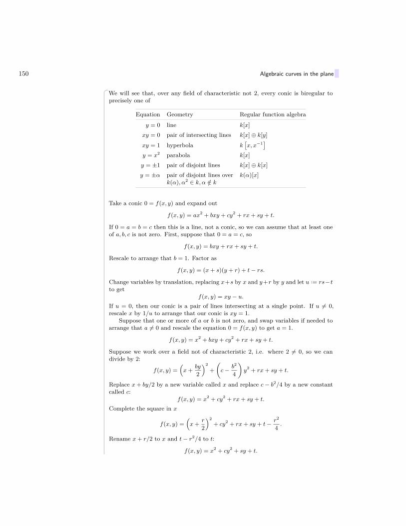
150 Algebraic curves in the plane

We will see that, over any field of characteristic not 2, every conic is biregular toprecisely one of

Equation Geometry Regular function algebra

y = 0 line k[x]xy = 0 pair of intersecting lines k[x]⊕ k[y]

xy = 1 hyperbola k[x, x−1]

y = x2 parabola k[x]y = ±1 pair of disjoint lines k[x]⊕ k[x]y = ±α pair of disjoint lines over k(α)[x]

k(α), α2 ∈ k, α /∈ k

Take a conic 0 = f(x, y) and expand out

f(x, y) = ax2 + bxy + cy2 + rx+ sy + t.

If 0 = a = b = c then this is a line, not a conic, so we can assume that at least oneof a, b, c is not zero. First, suppose that 0 = a = c, so

f(x, y) = bxy + rx+ sy + t.

Rescale to arrange that b = 1. Factor as

f(x, y) = (x+ s)(y + r) + t− rs.

Change variables by translation, replacing x+s by x and y+r by y and let u ..= rs−tto get

f(x, y) = xy − u.If u = 0, then our conic is a pair of lines intersecting at a single point. If u 6= 0,rescale x by 1/u to arrange that our conic is xy = 1.

Suppose that one or more of a or b is not zero, and swap variables if needed toarrange that a 6= 0 and rescale the equation 0 = f(x, y) to get a = 1.

f(x, y) = x2 + bxy + cy2 + rx+ sy + t.

Suppose we work over a field not of characteristic 2, i.e. where 2 6= 0, so we candivide by 2:

f(x, y) =(x+ by

2

)2+(c− b2

4

)y2 + rx+ sy + t.

Replace x+ by/2 by a new variable called x and replace c− b2/4 by a new constantcalled c:

f(x, y) = x2 + cy2 + rx+ sy + t.

Complete the square in x

f(x, y) =(x+ r

2

)2+ cy2 + rx+ sy + t− r2

4 .

Rename x+ r/2 to x and t− r2/4 to t:

f(x, y) = x2 + cy2 + sy + t.

Algebraic curves in the plane 151

If c = 0 thenf(x, y) = x2 + sy + t.

If s 6= 0 then replace sy + t by a new variable, which we call −y, to get

f(x, y) = x2 − y.

Note that then our curve is a parabola y = x2. On the parabola, every polynomialg(x, y) is just g

(x, x2), a polynomial in x. If 0 = s = t then our conic is actually a

line x = 0; linearly transform variable to get the conic to be y = 0. If 0 = s andt 6= 0 then our conic is x2 = −t. Again linearly transform to get the conic y2 = −t.If −t has a square root in k, say a, then our equation is y = ±a, and rescale the yvariable to get a = 1, so a pair of disjoint lines y = ±1. If −t has no square rootin k, then an empty set of points with coordinates in k, but a pair of disjoint lineswith coordinates in k(α), α =

√−t: y = ±α. This α is uniquely determined up to

scaling by an element of k×. For example, over the rational numbers, the equationsx2 = −t for t any prime or x2 = t for t any prime give conics with no rational points.Different primes give different conics, and the reader can work out why they are notbiregular over the rational numbers. One the other hand, over the real numbers, weonly have a single conic x2 = −1 with no real points.

A rational function on an algebraic curve X over a field k is a rational functionof x, y, whose denominator is not divisible by any nonconstant factor of the equationof the curve.

On the curve X = (y = x2), the rational function f = x/(x − y) might seem to beundefined near the origin, but we can also write it as

f = x

x− y ,

= x

x− x2 ,

= 11− x .

A rational function f is regular near a point of X if f can be written as f = b/cfor some polynomials b, c with c nonzero at that point.

A rational morphism of algebraic curves f : C → D is a map, which can be ex-pressed somehow as f(x, y) = (s(x, y), t(x, y)) for two rational functions s(x, y), t(x, y),each of which is regular at some point of C, so that f , applied to any point of C atwhich both s(x, y) and t(x, y) are regular, yields a point of D. A rational morphismwith a rational inverse is birational, and the associated curves are birational. A ratio-nal morphism is regular near a point of C if s(x, y) and t(x, y) are regular near thatpoint, i.e. can be expressed near that point as ratios of polynomials not vanishingnear that point.

Lemma 18.2. Algebraic curves in the plane (over any field) are birational just whentheir fields of rational functions are isomorphic.

Proof. Suppose that the curves are birational. Clearly the rational functions composewith the birational map, and with its inverse, identifying the fields. Conversely,suppose that the fields are isomorphic, say by an isomorphism

φ : k(C)→ k(D).

152 Algebraic curves in the plane

Write the coordinates of the plane in which C lives as x, y, and those of the plane inwhich D lives as u, v. Let s(x, y) ..= φ−1u and t(x, y) ..= φ−1v.

A curve birational to a line in the plane (with equation y = 0, for example) is arational curve. An algebraic curve C is rational just when k(C) ∼= k(x).

18.2 Imitate our picture of drawing lines through a point of y2 = x3+x2, but replacingthat cubic curve by an irreducible conic (curve of degree 2). Prove that conics arerational.

18.3 Prove that every algebraic curve over any algebraically closed field has infinitelymany points. Hints: Pick a point not on the curve. (You need to prove that such apoint exists, using the fact that every algebraically closed field is infinite.) Changevariables by translation to arrange that this point is the origin. Any line through theorigin strikes the curve at some point, except perhaps for finitely many exceptionallines. (Why?) Two lines through the origin intersect only at the origin. So any twolines through the origin strike the curve at different points. There are infinitely manylines through the origin. (Why?)

Integrals

Suppose that g(x, y) = 0 is the equation of an irreducible plane algebraic curve overthe field of real numbers, for example y2 = x2 +x3. Suppose that we can locally writethe curve as the graph of a function y = y(x), for example y =

√x2 + x3. Pick a

rational function f(x, y) on the curve, and consider the integral∫f dx, by which we

mean ∫f(x, y) dx =

∫f(x, y(x)) dx.

If the curve is rational, then we can parameterize it by x = x(t), y = y(t), as rationalfunctions of a new variable t. So then the integral becomes∫

f dx =∫f(x(t), y(t)) dx

dtdt

and this is a composition of rational functions, so a rational function of t. Using partialfractions, we can integrate this explicitly. For example, on the curve y2 = x2 + x3, ifwe take the rational function

f ..= x3

y,

we can write our integral as ∫f dx =

∫x3 dx√x2 + x3

.

We then solve this integral by parameterising as on page 147,

x = x(t) = t2 − 1, y = y(t) = t(t2 − 1

)

Ideals 153

to get ∫x3 dx√x2 + x3

=∫

x3 dx

y,

=∫ (

t2 − 1)3 2t dt

t (t2 − 1) ,

= 2∫ (

t2 − 1)2dt,

18.4 Simplify this integral completely into a function of x.

18.5 Recall that the circle is rational, as it can be parameterized by

x(t) = 1− t2

1 + t2, y(t) = 2t

1 + t2.

But the circle can also be parameterized using trigonometry:

x(θ) = cos θ, y(t) = sin θ.

Use these two facts to explain how to solve all integrals of the form∫f(cos θ, sin θ) dθ,

where f is any rational function.

Ideals

Given an algebraic curve C and a point p ∈ C (say, to be precise, that p ∈ C(k)is a point defined over k), we are naturally interested in the regular functions onC vanishing at p. If p has coordinates p = (x0, y0), then the polynomial functionsx−x0, y−y0 vanish simultaneously only at p. For simplicity, translate the plane so thatp lies at the origin. A regular function on C vanishes at p just when it is a sum xg(x, y)+yh(x, y), since every polynomial function vanishing at the origin is expressible in afinite Taylor series expansion. In other words, the regular functions on C vanishingat the origin are precisely the ideal I = (x, y). Similarly, the regular functions onC vanishing at (x, y) = (x0, y0) are the polynomials of the form (x− x0) g(x, y) +(y − y0)h(x, y), so constitute the ideal I = (x− x0, y − y0). This is the motivationfor the name “ideal”: an ideal is like a idealized notion of a point.

The regular functions on the real number line are the polynomials p(x), and thosewhich vanish at a point x = x0 are those of the form (x− x0) p(x). Similarly, if wetake two points x0 6= x1, then the regular functions on the line vanishing at bothpoints are the polynomials of the form (x− x0) (x− x1) p(x), the polynomials divisible(x− x0) (x− x1). If we imagine running the two points into one another, so that theycollide at x = 0, then these polynomials approach polynomials divisible by x2. Wecould think of the equation x2 = 0, or of the ideal I =

(x2), as representing a “double

point”.Working over k ..= Q on the curve C ..= (x2 = y), the ideal I ..= (x − 2) does

not correspond to any pointed defined over k. Again, we can think of I as an “idealpoint”.

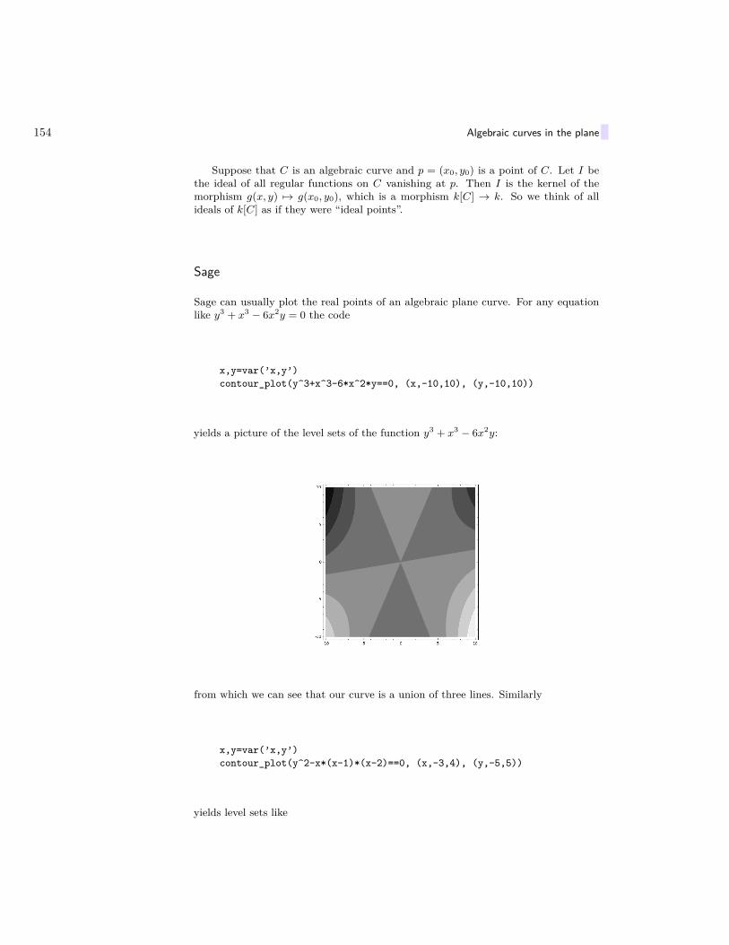
154 Algebraic curves in the plane

Suppose that C is an algebraic curve and p = (x0, y0) is a point of C. Let I bethe ideal of all regular functions on C vanishing at p. Then I is the kernel of themorphism g(x, y) 7→ g(x0, y0), which is a morphism k[C] → k. So we think of allideals of k[C] as if they were “ideal points”.

Sage

Sage can usually plot the real points of an algebraic plane curve. For any equationlike y3 + x3 − 6x2y = 0 the code

x,y=var(’x,y’)contour_plot(y^3+x^3-6*x^2*y==0, (x,-10,10), (y,-10,10))

yields a picture of the level sets of the function y3 + x3 − 6x2y:

from which we can see that our curve is a union of three lines. Similarly

x,y=var(’x,y’)contour_plot(y^2-x*(x-1)*(x-2)==0, (x,-3,4), (y,-5,5))

yields level sets like

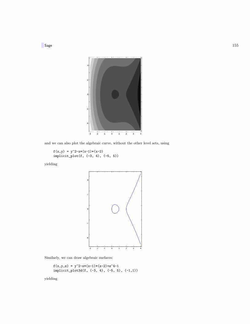
Sage 155

and we can also plot the algebraic curve, without the other level sets, using

f(x,y) = y^2-x*(x-1)*(x-2)implicit_plot(f, (-3, 4), (-5, 5))

yielding

Similarly, we can draw algebraic surfaces:

f(x,y,z) = y^2-x*(x-1)*(x-2)+z^4-1implicit_plot3d(f, (-3, 4), (-5, 5), (-1,1))

yielding

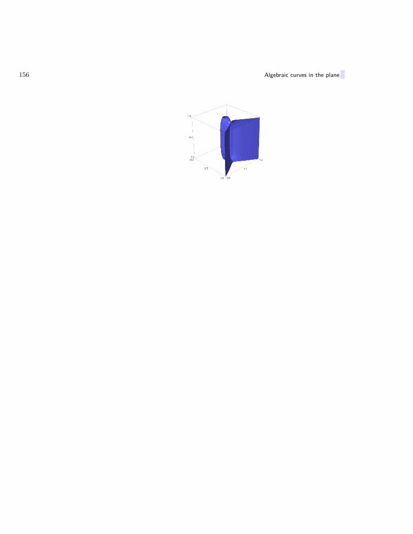
156 Algebraic curves in the plane

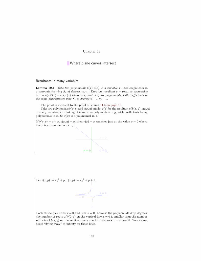
Chapter 19

Where plane curves intersect

Resultants in many variables

Lemma 19.1. Take two polynomials b(x), c(x) in a variable x, with coefficients ina commutative ring S, of degrees m,n. Then the resultant r = resb,c is expressibleas r = u(x)b(x) + v(x)c(x) where u(x) and v(x) are polynomials, with coefficients inthe same commutative ring S, of degrees n− 1,m− 1.

The proof is identical to the proof of lemma 11.3 on page 81.Take two polynomials b(x, y) and c(x, y) and let r(x) be the resultant of b(x, y), c(x, y)

in the y variable, so thinking of b and c as polynomials in y, with coefficients beingpolynomials in x. So r(x) is a polynomial in x.

If b(x, y) = y + x, c(x, y) = y, then r(x) = x vanishes just at the value x = 0 wherethere is a common factor: y.

b = 0

c = 0

r = 0

Let b(x, y) ..= xy2 + y, c(x, y) ..= xy2 + y + 1.

b = 0c = 0

Look at the picture at x = 0 and near x = 0: because the polynomials drop degrees,the number of roots of b(0, y) on the vertical line x = 0 is smaller than the numberof roots of b(a, y) on the vertical line x = a for constants x = a near 0. We can seeroots “flying away” to infinity on those lines.

157

158 Where plane curves intersect

b = 0c = 0

Finding the determinant of the associated 4× 4 matrix tells us that r(x) = x2, whichvanishes just at the value x = 0 where b(0, y) = y and c(0, y) = y+ 1 drop in degrees,not due to a common factor.

b = 0c = 0

The resultant of y and y+ 1 is not r(0) since the degrees drop, so we would computeresultant of y and y + 1 using a 2× 2 matrix, and find resultant −1.

If b(x, y) = xy2 + y and c(x, y) = 2xy2 + y+ 1 then r(x) = x(x+ 1) vanishes at x = 0and x = −1. At x = 0, b(0, y) = y, c(0, y) = y + 1 have no common factor, but dropdegrees. At x = −1, b(−1, y) = −y(y − 1), c(−1, y) = −2(y − 1)(y − 1/2) have acommon factor, but they don’t drop degrees.

b = 0c = 0

If b(x, y) = x2 +y2−1 and c(x, y) = (x−1)2 +y2−1 then r(x) = (2x−1)2 vanishes atx = 1/2, where there are two different intersection points, a double common factor:

b(1/2, y) = c(1/2, y) =(y −√

32

)(y +√

32

).

b = 0

c = 0

Resultants in many variables 159

Lemma 19.2. Suppose that k is a field and

x = (x1, x2, . . . , xn)

are variables and y is a variable. Take b(x, y) and c(x, y) two nonconstant polynomialsin k[x, y]. Then in some finite degree extension of k there are constants

λ = (λ1, λ2, . . . , λn)

so that in the expressions b(x+ λy, y) , c(x+ λy, y), the coefficients of highest orderin y are both nonzero constants.

Return to our earlier example of b(x, y) = xy2 + y and c(x, y) = 2xy2 + y+ 1 and let

B(x, y) ..= b(x+ λy, y) = λy3 + xy2 + y,

C(x, y) ..= c(x+ λy, y) = 2λy3 + 2xy2 + y + 1.

For any nonzero constant λ 6= 0, the resultant of B(x, y), C(x, y) is

r(x) = det

0 0 0 1 0 01 0 0 1 1 0x 1 0 2x 1 1l x 1 2λ 2x 10 l x 0 2λ 2x0 0 l 0 0 2λ

= −λ2 (λ+ 1 + x) .

So the resultant now vanishes just when x = −(λ + 1), which is precisely whenB(x, y), C(x, y) have a common factor of y − 1. With a small value of λ 6= 0, thepicture changes very slightly: we change x, y to x + λy, y, a linear transformationwhich leaves the x-axis alone, but tilts the y-axis to the left. Crucially, we tilt theasymptotic line at which the two curves approached one another (where b(x, y) andc(x, y) dropped degrees), but with essentially no effect on the intersection point:

B = 0C = 0

If b(x, y) = x2 + y2− 1 and c(x, y) = (x− 1)2 + y2− 1, then r(x) = (2x− 1)2 vanishesat x = 1/2, where there are two different intersection points.

b = 0

c = 0

If instead we pick any nonzero constant λ and let B(x, y) ..= (x+ λy)2 + y2 − 1 and

160 Where plane curves intersect

C(x, y) ..= (x+ λy − 1)2 + y2 − 1 then the resultant

r(x) = 4(λ2 + 1

)(x− 1 + λ

√3

2

)(x− 1− λ

√3

2

)vanishes at two distinct values of x corresponding to the two distinct roots. In thepicture, the two roots now lie on different vertical lines (different values of x).

B = 0C = 0

Proof. Write b as a sum of homogeneous polynomials of degrees 0, 1, 2, . . . , d, say

b = b0 + b1 + · · ·+ bd.

It is enough to prove the result for bd, so assume that b is homogeneous of degree d.The expression

b(x, 1)

is a nonzero polynomial over an infinite field, so doesn’t vanish everywhere by lemma 10.6on page 73. Pick λ to be a value of x for which b(λ, 1) 6= 0. Then

b(x+ λy, y) = yb(x, 1) + · · ·+ ydb(λ, 1).

Similarly for two polynomials b(x, y), b(x, y), or even for any finite set of polynomials.

Corollary 19.3. Take one variable y and several variables x = (x1, x2, . . . , xn)and two polynomials b(x, y) and c(x, y) over a field. Let r(x) be the resultant ofb(x, y), c(x, y) in the y variable. For any constant a in our field, if b(a, y) and c(a, y)have a common root in some algebraic extension of our field then r(a) = 0.

If the coefficient of highest order in y of both b(x, y) and c(x, y) is constant in x(for example, perhaps after the normalization described in lemma 19.2 on page 158)then r(a) = 0 at some value x = a in our field just exactly when b(a, y) and c(a, y)have a common factor. Moreover r(x) is then the zero polynomial just when b(x, y)and c(x, y) have a common factor which is a polynomial in x, y of positive degree in y.

Proof. If, at some value x = a, both the degrees of b(x, y) and c(x, y) don’t drop,then the resultant in y is expressed by the same expression whether we set x = a toa constant value or leave x as an abstract variable, compute resultant, and then setx = a.

Resultants in many variables 161

Work over the ring of polynomials in y, with coefficients rational in x. Theresultant in y being zero as a function of x forces a common factor in that ring, i.e.

b(x, y) = d(x, y)B(x, y),c(x, y) = d(x, y)C(x, y),

where d(x, y), B(x, y) and C(x, y) are rational in x and polynomial in y and d(x, y)has positive degree in y. In particular, c(x, y) factorises over that ring. By the Gausslemma (proposition 10.8 on page 74), c(x, y) factorises over the polynomials in x, y.But c(x, y) is irreducible, so one factor is constant, and it isn’t d(x, y), so it mustbe C(x, y), so we rescale by a nonzero constant to get d(x, y) = c(x, y), i.e. c(x, y)divides b(x, y).

Corollary 19.4. Given a finite collection of polynomial functions over a field k,for x = (x1, x2, . . . , xn), either

a. in some finite extension of k, there is at least one point on which all polynomialsin the collection vanish or

b. in some finite extension of k, every polynomial lies in the ideal generated bythis collection.

Proof. Suppose we just have two polynomials p1(x) and p2(x) in our collection. Asabove, after perhaps a finite extension, and a linear change of variables, we compute aresultant to find the values of one fewer of the variables on which there are simultaneouszeroes. The result follows by induction. Suppose instead that there are finitely manypolynomials in our collection. We repeatedly replace pairs by such resultants, toeventually reduce the number of variables, and apply induction on the variables. Inthe end, when we have only one variable: all resultants are constants, and if they arenot all zero, then there are no simultaneous solutions. Suppose that there is a nonzeroresultant in among these. Rescale to get its value to be 1. That nonzero resultantis expressed as a linear combination as in lemma 19.1 on page 157. By induction weconstruct polynomials qj(x) so that

1 = q1(x)p1(x) + q2p2(x) + · · ·+ qs(x)ps(x).

So 1 lies in the ideal generated by these p1(x), p2(x), . . . , ps(x). But then any polyno-mial f(x) has the form f(x) = f(x) · 1, so also lies in that ideal.

Chapter 20

Quotient rings

Recall once again that all of our rings are assumed to be commutative rings withidentity. Suppose that R is a ring and that I is an ideal. For any element r ∈ R, thentranslate of I by r, denoted r + I, is the set of all elements r + i for any i ∈ I.

If R = Z and I = 12Z is the multiples of 12, then 7 + I is the set of integers whichare 7 larger than a multiple of 12, i.e. the set of all numbers

. . . , 7− 12, 7, 7 + 12, 7 + 2 · 12, 7 + 3 · 12, . . .

which simplifies to. . . ,−5, 7, 19, 31, 53, . . .

But this is the same translate as −5 + I, since −15 + 12 = 7 so −5 + I is the set ofall numbers

. . . ,−5− 12,−5,−5 + 12,−5 + 2 · 12,−5 + 3 · 12, . . .

which is just. . . ,−15,−5, 7, 19, 31, 53, . . .

the same sequence.

Working again inside Z, 2 + 2Z = 2Z is the set of even integers.

If R = Q[x] and I = (x), then 12 + I is the set of all polynomials of the form

12 + xp(x)

for any polynomial p(x).

If i ∈ I then i+ I = I.

We add two translates by

(r1 + I) + (r2 + I) ..= (r1 + r2) + I,

and multiply by(r1 + I) (r2 + I) = (r1r2) + I.

Lemma 20.1. For any ideal I in any ring R, two translates a + I and b + I areequal just when a and b differ by an element of I.

Proof. We suppose that a+ I = b+ I. Clearly a belongs to a+ I, because 0 belongsto I. Therefore a belongs to a+ I = b+ I, i.e. a = b+ i for some i from I.

163

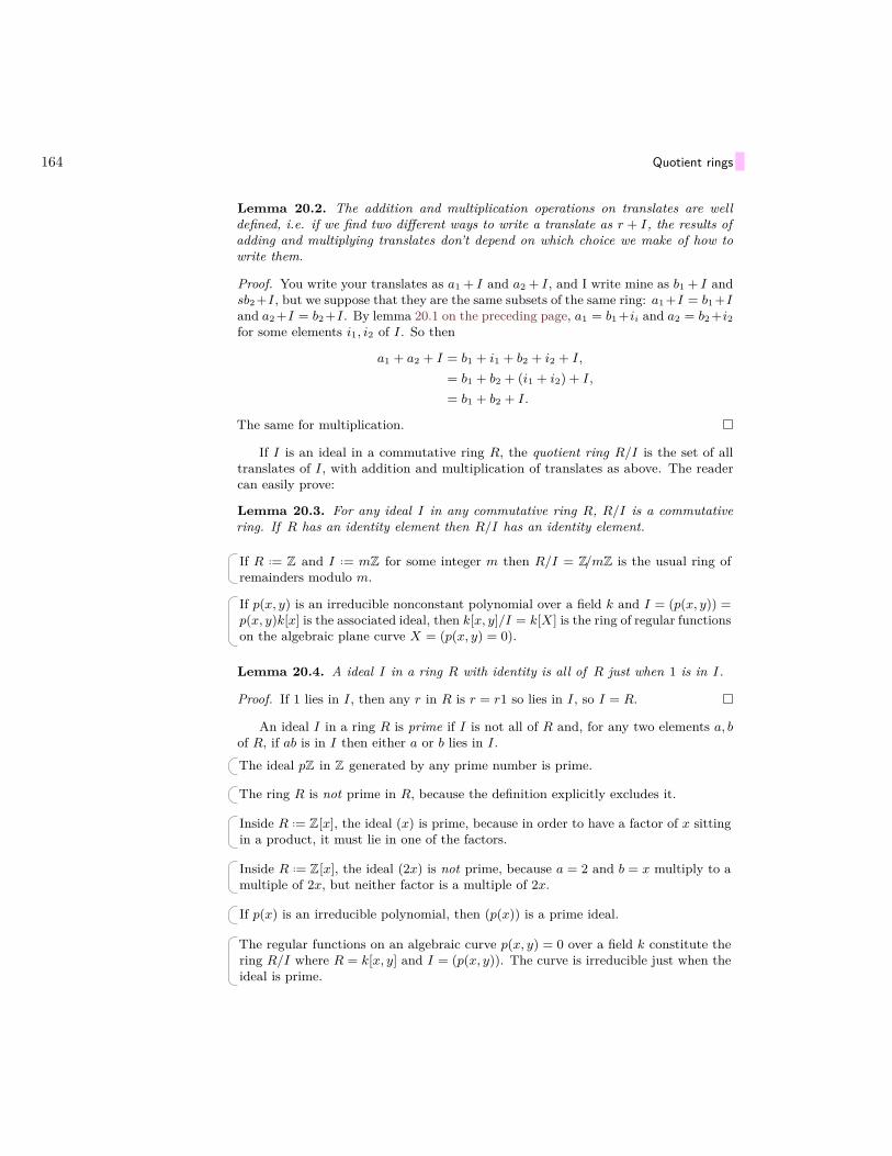
164 Quotient rings

Lemma 20.2. The addition and multiplication operations on translates are welldefined, i.e. if we find two different ways to write a translate as r + I, the results ofadding and multiplying translates don’t depend on which choice we make of how towrite them.

Proof. You write your translates as a1 + I and a2 + I, and I write mine as b1 + I andsb2 +I, but we suppose that they are the same subsets of the same ring: a1 +I = b1 +Iand a2 +I = b2 +I. By lemma 20.1 on the preceding page, a1 = b1 +ii and a2 = b2 +i2for some elements i1, i2 of I. So then

a1 + a2 + I = b1 + i1 + b2 + i2 + I,

= b1 + b2 + (i1 + i2) + I,

= b1 + b2 + I.

The same for multiplication.

If I is an ideal in a commutative ring R, the quotient ring R/I is the set of alltranslates of I, with addition and multiplication of translates as above. The readercan easily prove:

Lemma 20.3. For any ideal I in any commutative ring R, R/I is a commutativering. If R has an identity element then R/I has an identity element.

If R ..= Z and I ..= mZ for some integer m then R/I = Z/mZ is the usual ring ofremainders modulo m.

If p(x, y) is an irreducible nonconstant polynomial over a field k and I = (p(x, y)) =p(x, y)k[x] is the associated ideal, then k[x, y]/I = k[X] is the ring of regular functionson the algebraic plane curve X = (p(x, y) = 0).

Lemma 20.4. A ideal I in a ring R with identity is all of R just when 1 is in I.

Proof. If 1 lies in I, then any r in R is r = r1 so lies in I, so I = R.

An ideal I in a ring R is prime if I is not all of R and, for any two elements a, bof R, if ab is in I then either a or b lies in I.

The ideal pZ in Z generated by any prime number is prime.

The ring R is not prime in R, because the definition explicitly excludes it.

Inside R ..= Z[x], the ideal (x) is prime, because in order to have a factor of x sittingin a product, it must lie in one of the factors.

Inside R ..= Z[x], the ideal (2x) is not prime, because a = 2 and b = x multiply to amultiple of 2x, but neither factor is a multiple of 2x.

If p(x) is an irreducible polynomial, then (p(x)) is a prime ideal.

The regular functions on an algebraic curve p(x, y) = 0 over a field k constitute thering R/I where R = k[x, y] and I = (p(x, y)). The curve is irreducible just when theideal is prime.

Quotient rings 165

Take a field k. In the quotient ring R = k[x, y, z]/(z2 − xy), the ideal (z) containsz2 = xy, but does not contain x or y, so is not prime.

Lemma 20.5. An ideal I in a commutative ring with identity R is prime just whenR/I has no zero divisors, i.e. no nonzero elements α, β can have αβ = 0.

Proof. Write α and β as translates α = a+ I and β = b+ I. Then αβ = 0 just whenab+ I = I, i.e. just when ab lies in I. On the other hand, α = 0 just when a+ I = I,just when a is in I.

A ideal I in a ring R is maximal if I is not all of R but any ideal J which containsI is either equal to I or equal to R (nothing fits in between).

Lemma 20.6. If I is an ideal in a commutative ring R with identity, then I is amaximal ideal just when R/I is a field.

Proof. Suppose that I is a maximal ideal. Take any element α 6= 0 of R/I and writeit as a translate α = a + I. Since α 6= 0, a is not in I. We know that (a) + I = R,since I is maximal. But then 1 lies in (a) + I, so 1 = ab+ i for some b in R and i inI. Expand out to see that

1α

= b+ I.

So nonzero elements of R/I have reciprocals.Suppose instead that R/I is a field. Take an element a in R not in I. Then a+ I

has a reciprocal, say b+ I. But then ab+ I = 1 + I, so that ab = 1 + i for some i inI. So (a) + I contains (ab) + I = (1) = R.

If p is a prime number, then I ..= pZ is maximal in R ..= Z, because any other idealJ containing I and containing some other integer, say n, not a multiple of p, mustcontain the greatest common divisor of n and p, which is 1 since p is prime. Werecover the fact that Z/pZ is a field.

The ideals in R ..= Z/4Z are (0), (1) = Z/4Z and (2) ∼= Z/2Z, and the last of these ismaximal.

Take a field k and let R ..= k[x]. Every ideal I in R has the form I = (p(x)), becauseeach ideal is generated by the greatest common divisor of its elements. We have seenthat R/I is prime just when p(x) is irreducible. To further have R/I a field, we needI = (p(x)) to be maximal. Take some polynomial q(x) not belonging to I, so notdivisible by p(x). Since p(x) is irreducible, p(x) has no factors, so gcd {p(x), q(x)} = 1in k[x], so that the ideal generated by p(x), q(x) is all of R. Therefore I = (p(x)) ismaximal, and the quotient R/I = k[x]/(p(x)) is a field.

If k is an algebraically closed field and R ..= k[x] then every irreducible polynomialis linear, so every maximal ideal in R is I = (x− c) for some constant c.

20.1 For any positive integer m ≥ 2, what are the prime ideals in Z/mZ, and whatare the maximal ideals?

166 Quotient rings

Sage

We take the ring R = Q[x, y] and then quotient out by the ideal I = (x2y, xy3) toproduce the ring S = R/I. The generators x, y in R give rise to elements x+ I, y + Iin S, which are renamed to a, b for notational convenience.

R.<x,y> = PolynomialRing(QQ)I = R.ideal([x^2*y,x*y^3])S.<a,b> = R.quotient_ring(I)(a+b)^4

which yields a^4 + b^4.We can define R = Q[x, y], I = (y2), S = R/I where we label x+ I, y + I as a, b,

T = Q[z] and define a morphism φ : S → T by φ(a) = z3, φ(b) = 0:

R.<x,y> = PolynomialRing(QQ)I = R.ideal([y^2])S.<a,b> = R.quotient_ring(I)T.<z> = PolynomialRing(QQ)phi = S.hom([z^3, 0],T)phi(a^2+b^2)

yielding z6.

Automorphisms of splitting fields

Theorem 20.7. Suppose that k is a field and p(x) is a nonconstant polynomialover k, say of degree n. Any two splitting fields for p(x) over k are isomorphic by anisomorphism which is the identity on k.

Proof. We already know that splitting fields exist, by adding roots to irreduciblefactors of p(x). Each time we add a root, the dimension of the extension field over kis the degree of the irreducible factor. We then split off at least one linear factor inthe extension field, and repeat. So at most n! degree in total.

Given any splitting fieldK for an irreducible polynomial p(x), pick any root α ∈ Kof p(x) and map

f(x) ∈ k[x] 7→ f(α) ∈ K,to see that K ∼= k[x]/I. Hence K is uniquely determined up to isomorphism.

Suppose instead that p(x) is reducible, and that K,L are splitting fields of p(x).Pick an irreducible factor q(x) of p(x). Then the subfields of K,L generated by addinga root of q(x) to k are isomorphic, since q(x) is irreducible, so we can assume thatsubfields are the same field. We need only split p(x) over that field, or quotient outall copies of q(x) from p(x) and split the result. Apply induction on the degree ofp(x).

Adding a root to x2 + 1 over R yields the splitting field C.

Theorem 20.8. Suppose that K is a splitting field of an irreducible polynomial p(x)over a field k. If α, β ∈ K are roots of p(x) then the Galois group of K over k hasan element which takes α to β. In particular, K is a Galois extension of k.

Transcendental numbers 167

Proof. As in the proof of theorem 20.7 on the preceding page, there is a field isomor-phism k[x]/I → K taking x 7→ α, and another field isomorphism k[x]/I → K takingx 7→ β.

Transcendental numbers

A number α ∈ C is algebraic if it is the solution of a polynomial equation p(α) = 0where p(x) is a nonzero polynomial with rational coefficients. A number which is notalgebraic is called transcendental. More generally, given a field extension K of a fieldk, an element α ∈ K is algebraic over k if it is a root of a nonzero polynomial p(x)with coefficients in k.

Theorem 20.9. For any field extension K of a field k, an element α ∈ K is tran-scendental if and only if the field

k(α) ={p(α)q(α)

∣∣∣∣ p(x)q(x) ∈ k(x) and q(α) 6= 0

}is isomorphic to k(x).

Proof. If α is transcendental, then the map

f : p(x)q(x) ∈ k(x) 7→ p(α)

q(α) ∈ k(α)

is clearly well defined, onto, and preserves all arithmetic operations. To show that fis 1-1 is the same as showing that f has trivial kernel. Suppose that p(x)/q(x) lies inthe kernel of f . Then p(α) = 0, so p(x) = 0, so p(x)/q(x) = 0. So the kernel is trivial,and so f is a bijection preserving all arithmetic operations, so f is an isomorphism offields.

On the other hand, take a element α in K and suppose that there is some isomor-phism of fields

g : k(x)→ k(α).

Let β ..= g(x). Because g is a field isomorphism, all arithmetic operations carried outon x must then be matched up with arithmetic operations carried out on β, so

g

(p(x)q(x)

)= p(β)q(β) .

Because g is an isomorphism, some element must map to α, say

g

(p0(x)q0(x)

)= α.

Sop0(β)q0(β) = α.

So k(β) = k(α). Any algebraic relation on α clearly gives one on β and vice versa.Therefore α is algebraic if and only if β is. Suppose that β is algebraic. Then q(β) = 0for some polynomial q(x), and then g is not defined on 1/q(x), a contradiction.

168 Quotient rings

Finite fields

We are going to make a complete list of all finite fields. Pick a prime number p andwork over the field k = Z/pZ. For any integer n > 0, the polynomial xp

n

− x has twoobvious linear factors: x and x− 1, and then factors as

xpn

− x = x(x− 1)(x−2+pn

+ x−3+pn

+ · · ·+ x+ 1).

Lemma 20.10. For any prime p, over any extension field K of the field k = Z/pZ,the polynomial

xpn

− x

has no multiple roots.

Proof. Let c(x) ..= xpn

−x. As above, write x(x−1)b(x) = c(x). Note that b(0) = 1 6= 0and b(1) = pn − 1 = −1 6= 0. If, in some field K, we can factor out a multiple rootfrom b(x), that multiple root is not at x = 0 or x = 1, so we can factor out the samemultiple root from c(x) = x(x− 1)b(x). Take the derivative of c(x):

c′(x) = d

dx

(xp

n

− x)

= pnx−1+pn

− 1 = −1,

since p = 0 in k. But then c′(x) has no roots in any field extension K of k, so c(x)has no multiple roots over K, so b(x) has no multiple roots over K.

Lemma 20.11. For any finite field k of characteristic p, the Frobenius morphismf(x) = xp is an automorphism of fields f : k → k, i.e. is a bijection preservingaddition, subtraction, multiplication and division, taking 0 7→ 0 and 1 7→ 1.

Proof. Clearly 0p = 0 and 1p = 1. For any b, c ∈ k, clearly (bc)p) = bpcp. Thebinomial theorem gives

(b+ c)p = bp + pbp−1c+ p(p− 1)2 bp−2c2 + · · ·+ p!

j!(p− j)! bp−jcj + · · ·+ c.

Every term except b and c has a factor of p in it, and p = 0 in k, so

(b+ c)p = bp + cp.

The same for (b− c)p = bp − cp. If f(b) = 0, then bp = 0 so b · bp−1 = 0 so b = 0 orbp−1 = 0, and by induction, we find that b = 0. If f(b) = f(c) then f(b − c) = 0 sob− c = 0 so b = c, i.e. f is 1-1. But then, since k is finite, f is a bijection.

Theorem 20.12. For any prime p, the splitting field K of the polynomial

c(x) = xpn

− x

over the field k = Z/pZ has pn elements, every one of which is a root of c(x). Everyfinite field K is obtained uniquely as the splitting field of c(x) for some prime number pand integer n ≥ 1, and so is uniquely determined up to isomorphism by its number ofelements pn.

Finite fields 169

Proof. There are pn roots of c(x) = xpn

−x over its splitting field K, since b(x) splitsinto linear factors, and, by lemma 20.10 on the facing page each linear factor gives adistinct root. Given any roots α, β of c(x),

αpn

= α, βpn

= β.

Apply the Frobenius morphism:

(α+ β)pn

= αpn

+ βpn

= α+ β,

so c(α+ β) = 0. Similarly

(αβ)pn

= αpn

βpn

= αβ,

so c(αβ) = 0. Hence the roots of c(x) form a field, over which c(x) splits, and so b(x)splits. So every element of K is a root of c(x), and so K is a splitting field of c(x)with pn elements. By the existence and uniqueness of splitting fields in theorem 20.7on page 166, K is the unique splitting field of c(x).

Take any finite field L, say of characteristic p. We map 0, 1, 2, . . . , p−1 in k = Z/pZto 0, 1, 2, . . . , p−1 in L, a morphism of fields. Hence L is a vector space over k, of finitedimension, say n, and so has pn elements. The Frobenius morphism is an invertiblek-linear map of L, generating a subgroup of the group of invertible k-linear mapsL→ L. This subgroup is finite, since there are only finitely many elements of L, sofinitely many permutations of those elements. This subgroup is generated by a singleelement, so is cyclic. By theorem 12.2 on page 98, this subgroup is isomorphic to Z/`Z,for some integer ` > 0, so every element of L satisfies some equation xp

`

= x.

For any finite field k, say with pn elements, we can associate to any α, β ∈ k thequadratic equation (x−α)(x−β) = 0 which has roots α, β. On the other hand, givena quadratic equation x2 + bx + c = 0, we can ask whether it has roots. Those withroots are given as x2 + bx+ c = (x− α)(x− β) for some α, β, unique up to swappingthe order in which we write them down. As there are pn elements, there are

pn(pn + 1)2

pairs α, β of possible roots, up to swapping order. But there are p2n quadraticequations x2 + bx+ c: choose any b, c from k. So

p2n − pn(pn + 1)2 = pn(pn − 1)

2

quadratic equations over k have no solution in k.In particular, let k1 ⊂ k2 ⊂ k3 . . . be finite fields or orders 2, 4, 8 and so on. Each

kn+1 is the splitting field of the polynomial z2 + z+α over kn where α is any elementof kn not belonging to kn−1. In particular, we can see which quadratic equationshave solutions in which fields of characteristic 2. Note that we can’t use the quadraticformula in fields of characteristic 2, because the quadratic formula has a 2 in it.

20.2 Prove by induction that if k is a finite field of characteristic 2, then every elementα of k is a square, i.e. α = β2 for some β.

170 Quotient rings

Sage

Lets get sage to construct the splitting field K of p(x) ..= x2 + x + 1 over the fieldk = Z/2Z. Sage constructs splitting fields by first building a ring, which we will callR, of polynomials over a field. In our case, we build R = k[x]. Then we let K be thefield generated by an element a, which corresponds to the variable x in the polynomialring R.

R.<x> = PolynomialRing(GF(2))K.<a> = (x^2 + x + 1).splitting_field()

We can then make a list of some elements of K, call it S, and compute out additionand multiplication tables:

S=[0,1,a,a+1]print("Addition table:")for i in range(0,4):

for j in range(0,4):print("({})+({})={}".format(S[i],S[j],S[i]+S[j]))

print("Multiplication table:")for i in range(0,4):

for j in range(0,4):print("({})*({})={}".format(S[i],S[j],S[i]*S[j]))

Chapter 21

Field extensions and algebraic curves

We can sometimes draw pictures of field extensions. Take an algebraic curve C =(p(x, y) = 0) in the plane, and look at its field of rational functions k(C), our favouriteexample of a field extension of a field k.

Suppose that K is a field extension of k(C), say K = k(C)(α) given by extending byan element α. We want to draw a curve D so that K = k(D).

If α is transcendental, then k(C)(α) ∼= k(C)(z) for some abstract variable z. Butk(C) is already a field of rational functions of two variables x, y, quotiented out toenforce the relation p(x, y) = 0. So K is just the rational functions on the “cylinder”C × k inside 3-dimensional space, with variables x, y, z; our cylinder has the equationp(x, y) = 0, independent of z.

Suppose instead that α is algebraic, say satisfying a polynomial equation f(z) = 0with f(z) a polynomial with coefficients from k(C). So each coefficient of f(z) is itselfa rational function on C. Each such function is expressible as a rational functionof x, y. Clearing denominators, we get a polynomial equation f(x, y, z) = 0 withcoefficients in the underlying field k. The solutions form a surface in 3-dimensionalspace. But the resulting surface depends on how we pick out rational functions ofx, y to represent our coefficients of f(z) from k(C). So in fact we have to restrict

171

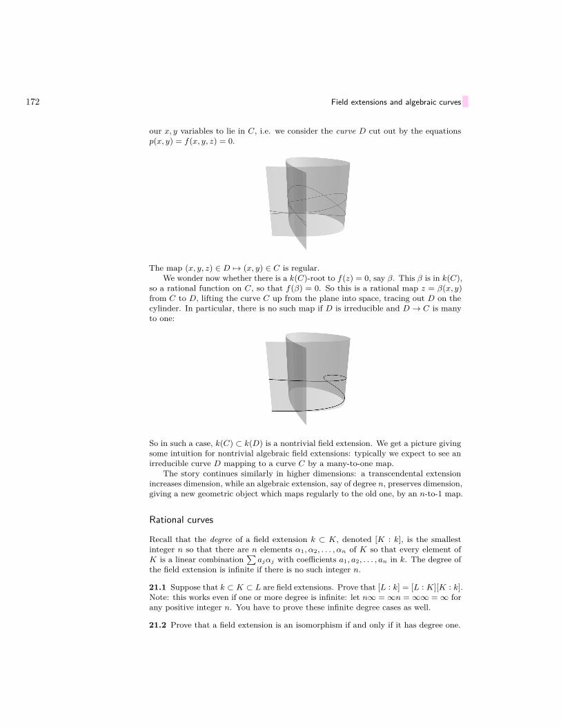
172 Field extensions and algebraic curves

our x, y variables to lie in C, i.e. we consider the curve D cut out by the equationsp(x, y) = f(x, y, z) = 0.

The map (x, y, z) ∈ D 7→ (x, y) ∈ C is regular.We wonder now whether there is a k(C)-root to f(z) = 0, say β. This β is in k(C),

so a rational function on C, so that f(β) = 0. So this is a rational map z = β(x, y)from C to D, lifting the curve C up from the plane into space, tracing out D on thecylinder. In particular, there is no such map if D is irreducible and D → C is manyto one:

So in such a case, k(C) ⊂ k(D) is a nontrivial field extension. We get a picture givingsome intuition for nontrivial algebraic field extensions: typically we expect to see anirreducible curve D mapping to a curve C by a many-to-one map.

The story continues similarly in higher dimensions: a transcendental extensionincreases dimension, while an algebraic extension, say of degree n, preserves dimension,giving a new geometric object which maps regularly to the old one, by an n-to-1 map.

Rational curves

Recall that the degree of a field extension k ⊂ K, denoted [K : k], is the smallestinteger n so that there are n elements α1, α2, . . . , αn of K so that every element ofK is a linear combination

∑ajαj with coefficients a1, a2, . . . , an in k. The degree of

the field extension is infinite if there is no such integer n.

21.1 Suppose that k ⊂ K ⊂ L are field extensions. Prove that [L : k] = [L : K][K : k].Note: this works even if one or more degree is infinite: let n∞ =∞n =∞∞ =∞ forany positive integer n. You have to prove these infinite degree cases as well.

21.2 Prove that a field extension is an isomorphism if and only if it has degree one.

Rational curves 173

21.3 Suppose that p(x) is an irreducible polynomial over a field k. Let K ..=k[x]/(p(x)). Prove that [K : k] is the degree of p(x).

21.4 Prove that if u(t) is a nonconstant rational function over a field k, then thereare infinitely many values of u(t) as t varies over k. In particular, k ⊂ k(u(t)) is atranscendental extension.

Recall that a curve C = (0 = f(x, y)) is irreducible if f(x, y) is irreducible.

Theorem 21.1. An irreducible plane algebraic curve C is rational just when thereis a nonconstant rational map L→ C. In other words, C is rational just when thereare rational functions x(t), y(t) for which the point (x(t), y(t)) lies in C for all t inthe algebraic closure of the field.

Proof. If our curve C is rational then by definition C is birational to a line, so there issuch a map. Suppose on the other hand that there is such a map L→ C, say writtenas t ∈ L 7→ (x(t), y(t)) ∈ C with

f(x(t), y(t)) = 0

for some rational functions x(t), y(t), not both constant. As we vary t through k, themoving point (x(t), y(t)) moves through infinitely many different points of the plane.Take a rational function on C, say g(x, y) = b(x, y)/c(x, y). Then c(x, y) 6= 0 at allbut finitely points of C. (Note that this requires that our curve C is irreducible, asotherwise we might have g(x, y) vanishing on a component of C.) So at infinitely manyvalues of t, g(x(t), y(t)) is defined. We map g(x, y) ∈ k(X) 7→ g(x(t), y(t)) ∈ k(t), amorphism of fields. The image is some subfield K = k(x(t), y(t)) ⊂ k(t). The resultfollows from the following theorem applied to K.

Theorem 21.2 (Lüroth’s theorem). Suppose that K ⊂ k(t) is a finitely generatedextension of a field k, where t is an abstract variable. Then K = k(f(t)) is generatedby a single rational function f(t) in k(t). In particular, either K = k (if f(t) is aconstant function) or K is isomorphic to k(t) by t 7→ f(t).

The proof of this theorem requires a lemma:

Lemma 21.3. Take a nonconstant rational function f(x) = b(x)/c(x), with b(x), c(x)coprime, over a field k. Then, as a polynomial in a variable y with coefficients ink(f(x)), the expression

f(x)c(y)− b(y)in k(f(x))[y] is irreducible.

Proof. This expression is not zero, because it is nonconstant in x. It vanishes at y = x.Hence x satisfies this polynomial (in y) expression with coefficients in k(f(x)). So k(x)is an algebraic extension of k(f(x)). Since k(x) is transcendental over k, k(f(x)) istranscendental over k. So f(x) solves no polynomial equation over k, and so taking anyabstract variable t and mapping k(t, y)→ k(f(x), y) by t 7→ f(x) gives an isomorphismof fields, and similarly k[t, y] → k[f(x), y] is an isomorphism of rings. By Gauss’slemma (proposition 10.8 on page 74), to show that tc(y)−b(y) is irreducible in k(t)[y],it suffices to prove that it is irreducible in k[t, y], i.e. clear t from denominators. Ifwe can factor tc(y) − b(y) = g(t, y)h(t, y) in k[t, y] then one of g(t, y) or h(t, y) hasdegree 1 in t, since the product does, and so one of g(t, y) or h(t, y) has degree zero

174 Field extensions and algebraic curves

in t, depending only on y, say g(t, y) = g(y). Then g(t)h(t, y) = tc(y)− b(y), so g(y)divides tc(y) − b(y), and since t is an abstract variable, g(y) divides b(y) and c(y),which are coprime, so g(y) is a nonzero constant.

We now prove Lüroth’s theorem:

Proof. For each element f(t) = b(t)/c(t) in K, let n be the larger of the degrees ofb(t), c(t). Pick an element f(t) = b(t)/c(t) in K, not in k, for which the value of n isas small as possible. By the previous lemma, the polynomial B(y) = f(x)c(y)− b(y)is irreducible in k(f(x))[y], so the map

x, y ∈ k(f(x))[y]/(B(y)) 7→ x, x ∈ k(x)

is an isomorphism of fields and [k(x) : k(f(x))] = n. The expression B(y) is thepolynomial in K[y] of smallest positive y-degree which is satisfied by y = x, since asmaller degree one would give a smaller value for n. Indeed the y-degree of B(y) is n.In particular, B(y) is also irreducible in K[y] and the map

x, y ∈ K[y]/(B(y)) 7→ x, x ∈ k(x)

is an isomorphism. In particular, [k(x) : K] = n. But

n = [k(x) : k(f(x))],= [k(x) : K][K : k(f(x))],= n[K : k(f(x))]

so [K : k(f(x))] = 1.

Chapter 22

The projective plane

The more systematic course in the present introductory memoir . . . wouldhave been to ignore altogether the notions of distance and metrical ge-ometry . . . . Metrical geometry is a part of descriptive geometry, anddescriptive geometry is all geometry.

— Arthur Cayley

The old fashioned term descriptive geometry means the geometry of straight lines.Straight lines in the plane remain straight when you rescale the plane, or translatethe plane to the left or right, up or down, or when you rotate the plane. They evenremain straight when you carry out any linear change of variables, as you know fromlinear algebra.

To see a World in a Grain of Sand,And Heaven in a Wild Flower.Hold Infinity in the palm of your hand,And Eternity in an hour.

— William BlakeAuguries of Innocence

Railway tracks built on a flat plane appear to meet “at infinity”.

Creative CommonsAttribution-Share Alike 3.0Unported license. I, MarcusObal

Imagine that we were to add a point to the plane “at infinity” in the direction wherethese tracks (straight lines) appear to meet. Danger: in order to add only one point,imagine that the two rails meet at the same point in one direction as they do in theother, making them both into circles. The projective plane is the set of all of theusual points of the plane (which we can think of as the “finite points” of the projectiveplane) together with some sort of “points at infinity” to represent the directions inthe plane.

175

176 The projective plane

But you must note this: if God exists and if He really did create the world,then, as we all know, He created it according to the geometry of Euclidand the human mind with the conception of only three dimensions inspace. Yet there have been and still are geometricians and philosophers,and even some of the most distinguished, who doubt whether the wholeuniverse, or to speak more widely the whole of being, was only created inEuclid’s geometry; they even dare to dream that two parallel lines, whichaccording to Euclid can never meet on earth, may meet somewhere ininfinity.

— Fyodor DostoyevskyThe Brothers Karamazov

We would like a more precise mathematical definition of points “at infinity”. Placeyourself at a vantage point above the plane.

Every “finite” point of the plane lies on a line through your vantage point: the lineof sight.

You can also look out to the points at infinity, along lines:

For example, there is such a line parallel to the lines of our train track:

The projective plane 177

On the other hand, if we take any line through the vantage point, either it hits a“finite” point of the plane:

or it is parallel to the plane

so that it is pointed along the direction of some train tracks (lines) in the plane, tosome “point at infinity”.

The points of the projective plane, finite points together with infinite points at infinity,are in 1-1 correspondence with lines through the vantage point.

This picture gives us a rigorous definition of points at infinity: the projective planeis the set of all lines through a chosen point of 3-dimensional space, called the vantagepoint. The points of the projective plane (using this definition) are the lines throughthe vantage point. The “finite points” are the lines not parallel to the horizontalplane, while the “infinite points” are the lines which are parallel the horizontal plane.The lines, also called projective lines, of the projective plane are the planes throughthe vantage point.

178 The projective plane

Homogeneous coordinates

We can make this more explicit by writing each point of 3-dimensional space R3 as atriple (x, y, z). Draw the plane not as the usual xy-plane, but as the plane z = z0, forsome nonzero constant z0. Take the vantage point to be the origin. Any linear changeof the 3 variables x, y, z takes lines (and planes) through the origin to one another:there are more symmetries of the projective plane than we encountered before.

Every point of 3-dimensional space not at the origin lies on a unique line throughthe origin. So every point (x, y, z) with not all of x, y, z zero lines on a unique linethrough the origin. The points of this line are precisely the rescalings (tx, ty, tz) ofthat point. So each point of the projective plane can be written as a triple (x, y, z),not all zero, and two such triples represent the same point just when each is a rescalingof the other. Denote such a point as [x, y, z]. For example, the point [3, 1, 2] of theprojective plane means the line through the origin consisting of the points of the form(3t, t, 2t) for all values of a variable t, including (3, 1, 2), (3 · 2, 1 · 2, 2 · 2), (−3,−1,−2),and so on. We write this as:

[3, 1, 2] = [3 · 2, 1 · 2, 2 · 2] = [−3,−1,−2].

The coordinates x, y, z are the homogeneous coordinates of a point [x, y, z] of theprojective plane.

In our pictures, the plane z = z0 was below the vantage point, but it is moretraditional to take the plane to be z = 1, above the vantage point. The affine plane isjust the usual xy plane, but identified either with the plane z = 1, or with the subsetof the projective plane given by points [x, y, 1].

The roles of x, y, z are all the same now, and we can see that any linear change ofvariables of x, y, z takes the points of the projective plane to one another, and takesthe lines of the projective plane to one another. Each linear change of variables isrepresented by an invertible matrix

g =

(g00 g01 g02g10 g11 g12g20 g21 g22

).

Conventionally we label our matrix columns using 0, 1, 2 rather than 1, 2, 3. Such amatrix takes a point p = [x, y, z] of the plane to the point q = [X,Y, Z] where(

XYZ

)= g

(xyz

).

We denote this relation as q = [g]p and call [g] a projective automorphism. Clearlyif g and h are 2 invertible 3 × 3 matrices, then [gh] = [g][h], i.e. we carry out thetransformation of lines through the origin by carrying out the multiplications by thematrices.

Lemma 22.1. If a square matrix g rescales every nonzero vector by a scalar, i.e.gx = λ(x)x for some number λ(x), for every vector x 6= 0, then λ(x) is a constantscalar independent of x.

Proof. Suppose that g is n×n. If n = 1 then every square matrix is a constant scalar,so suppose that n ≥ 2. Write our vectors as x =

∑jxjej in the standard basis of Rn

Example: the Fano plane 179

and calculate

gx = λ(x)x,

=∑j

λ(x)xjej ,

=∑j

xjgej ,

=∑j

xjλ(ej) ej .

So for any x with xj 6= 0, we have λ(x) = λ(ej). But then if xi 6= 0, and if i 6= j, then

λ(x) = λ(ei) ,= λ(ei + ej) ,= λ(ej) .

So λ is a constant.

Lemma 22.2. Two projective automorphisms [g], [h] have precisely the same effecton all points [x, y, z] of the projective plane just when the matrices agree up to aconstant h = λg, some number λ 6= 0.

Proof. Let ` ..= h−1g, so that [`] = [h]−1[g] and [`] fixes every point of the projectiveplane just when ` rescales every vector in R3 by a scalar.

In particular, the points of the projective plane are permuted by the projectiveautomorphisms, as are the projective lines.

The projective plane over any field k, denoted P2(k), is the set of lines through theorigin in k3. In k3, the line through two points

p =

(xyz

), q =

(XYZ

)

is just the set of all points tp+ (1− t)q for t in k.

Example: the Fano plane

Let k ..= Z/2Z; the Fano plane is the projective plane P2(k). Each point is [x, y, z]with x, y, z in k defined up to rescaling. But the only nonzero scalar you can use torescale with is 1, since k = { 0, 1 }. Therefore we can just write [x, y, z] as (x, y, z).Taking all possibilities for x, y, z from k, not all zero, we get 7 points[1

00

],

[010

],

[110

],

[001

],

[101

],

[011

],

[111

],

corresponding to the numbers 1, 2, . . . , 7 written in base 2.We can also draw this diagram as a cube; for each point, you draw the correspond-

ing point in R3 with the same coordinates:

180 The projective plane

6

3

57

1

4

2

with one vertex not marked. The unmarked vertex If we let k ..= Z/2Z, then the cubeis the set of points in k3, or more precisely, since the unlabelled point is the originand is deleted, the cube is the Fano plane. Every line in the Fano plane has threevertices. Take two numbers from 1 to 7, say 1, 5, and write out their binary digitsunder one another:

001101.

Look at these as vectors in k3, so add them without carrying digits:

001101

100

The sum vector lies on the same line in the Fano plane, giving the lines:

6

3

57

1

4

2

6

3

57

1

4

2

6

3

57

1

4

2

6

3

57

1

4

2

6

3

57

1

4

2

6

3

5

7 1

4

2

6

3

5

1

4

2

Projective space

Similarly, projective space Pn(k) is the set of lines through the origin of kn+1, anda projective automorphism of projective space is the result of applying an invertiblesquare matrix to those lines. Again, two invertible square matrices yield the sameprojective automorphism just when they agree up to a scalar multiple, by the sameproof.

Chapter 23

Algebraic curves in the projective plane

Homogenisation of plane curves

Take an algebraic curve y2 = x2 + x3 in the affine plane over a field k.

The cone on the curve is the surface in k3 given by y2z = x2z + x3.

The recipe: given an algebraic equation, like y2 = x2 + x3:a. Find the degree n of the highest term; in this example n = 3.b. Invent a new variable z.c. Multiply each term by a power of z so that the total degree of each term reaches

n.A polynomial is homogeneous if all of its terms have the same total degree, i.e. sumof degrees in all variables.

23.1 Homogenise x2y − x2 + y = 1 + 2x− y2x3.

In sage:

R.<x,y,z> = PolynomialRing(QQ)p = x^3+x*y+1p.homogenize(z)

yields x3 + xyz + z3.The homogenised polynomial equation y2z = xz2 + x3 has all terms of degree

3, so if we rescale x, y, z to tx, ty, tz, we rescale both sides of the equation by t3, so

181

182 Algebraic curves in the projective plane

solutions (x, y, z) rescaled remain solutions (tx, ty, tz). Thefore every solution lies ona line through the origin consisting of other solutions. The set of solutions is a surface,which is a union of lines through the origin. A projective plane curve is the set oflines through the origin satisfying a nonzero homogeneous polynomial.

Conics

Take a hyperbola xy = 1 in the affine plane,

−5

−5

x

y

and homogenise to xy = z2, as we see from three different perspectives:

If we slice the surface along a plane like z = 2, parallel to the plane we drew buthigher up, that plane z = 2 intersects our surface in a dilated hyperbola. But if weslice the surface along the plane x = 1, we get xy = z2 to become y = z2, a parabola:

Conics 183

Suitable linear changes of variable interchange the x and z axes, so suitable projectiveautomorphisms identify the two affine curves: the hyperbola and the parabola. Inparticular, the two curves have isomorphic fields of rational functions. They don’thave isomorphic rings of regular functions.

If instead we slice our surface with the plane x+ y = 1,

we get y = 1− x plugged in to xy = z2, which simplifies to(x− 1

2

)2+ z2 = 1

4 ,

a circle of radius 12 . So again the circle is birational to the parabola and to the

hyperbola, and they all have the same rational function fields. In these pictures wecan see why the conics are called conics: they are all slices of the same cone.

The affine curve x2 + y2 = −1 has no real points on it, but has complex points. Ithomogenises to x2 + y2 + z2 = 0, a “sphere of zero radius”, with the origin as itsonly real point, but with again many complex points. The complex linear changeof variables X = x− iy, Y = x+ iy, Z = iz gives us XY = Z2, the same projectivecurve as before. So these curves are all birational over the complex numbers, andindeed are all identified by automorphisms of the complex projective plane.

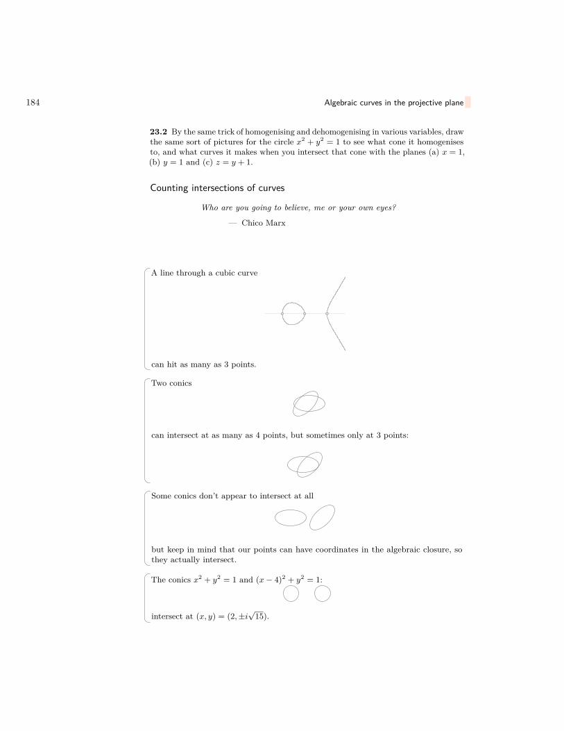
184 Algebraic curves in the projective plane

23.2 By the same trick of homogenising and dehomogenising in various variables, drawthe same sort of pictures for the circle x2 + y2 = 1 to see what cone it homogenisesto, and what curves it makes when you intersect that cone with the planes (a) x = 1,(b) y = 1 and (c) z = y + 1.

Counting intersections of curves

Who are you going to believe, me or your own eyes?

— Chico Marx

A line through a cubic curve

can hit as many as 3 points.

Two conics

can intersect at as many as 4 points, but sometimes only at 3 points:

Some conics don’t appear to intersect at all

but keep in mind that our points can have coordinates in the algebraic closure, sothey actually intersect.

The conics x2 + y2 = 1 and (x− 4)2 + y2 = 1:

intersect at (x, y) = (2,±i√

15).

Counting intersections of curves 185

Some conics appear not to have even complex intersections, such as x2 + y2 = 1 andx2 + y2 = 2.

But in the projective plane, we can homogenise to x2 + y2 = z2 and x2 + y2 = 2z2,and then intersect with the plane x = 1, to get 1 + y2 = z2 and 1 + y2 = 2z2, whichintersect at (y, z) = (±i, 0).

23.3 Find all points of the curve x3 + x2y+ xy2 + y3 + x2 = 1 which lie “at infinity”,i.e. on the line z = 0 in homogeneous coordinates, over the field k = C.

23.4 Find all points of the curve y2 + y = x3 + x+ 1 on the projective plane over thefield k = Z/5Z.

Lemma 23.1. Suppose that k is an infinite field. Then for any finite set of linesin P2(k), there are infinitely many points of P2(k) not on any of those lines.

Proof. If we work in the affine plane, the points (x, y) lying on those lines must satisfyone of the associated linear equations, say y = mix + bi or x = ci. Pick a numberx0 not among the constants ci. Now we have finitely many values y = mix0 + bi toavoid; pick y to not be one of those.

Lemma 23.2. Every nonzero homogeneous polynomial of degree n in two variablesover a field k has n roots, counted with multiplicities, in P1(k), and so splits into aproduct of homogeneous linear factors over k.

Proof. As part of the proof, we define multiplicities of zeroes of a homogeneouspolynomial p(x, y) to be multiplicities of linear factors. So we are saying preciselythat p(x, y) factors into n linear factors. If p(x, y) has a linear factor, divide it outand apply induction. Since y is not a linear factor of p(x, y), p(x, 1) has degree n, sayp(x, 1) = a(x− x1) . . . (x− xn). The homogeneous polynomial

r(x, y) ..= p(x, y)− a(x− x1y)(x− x2y) . . . (x− xny)

vanishes at y = 1 for any x, so by homogeneity vanishes for any y 6= 0. Fixing anyvalue of x, there are infinitely many values of y at which 0 = r(x, y), and so r(x, y)vanishes everywhere.

The polynomialp(x, y) = x3 + x2y − 2xy2

becomesp(x, 1) = x3 + x2 − 2x = x(x− 1)(x+ 2),

so thatp(x, y) = x(x− y)(x+ 2y).

The family of curves with y2 = ax contains the curve y2 = 0 when a = 0, a line. Soa family of curves of degree 2 contains a curve of degree 1. It is natural to think ofthe curve being a “double line” when a = 0.

186 Algebraic curves in the projective plane

Similarly, we can say that a multiple component of a curve means a curve givenby an equation which is a positive integer power of an irreducible homogeneous poly-nomial, say 0 = f(x, y, z)k giving a component with multiplicity k. From now on, weallow projective plane curves to have components with positive integer multiplicities.

Breaking curves into components

Theorem 23.3 (Study). Every algebraic curve in the projective plane has a uniquedecomposition into irreducible algebraic curves, its components. To be more precise,every nonzero homogeneous polynomial in 3 variables f(x, y, z) has a decomposition

f = a0gk11 gk2

2 . . . gknn ,

into a product of a nonzero constant a0 and several coprime irreducible homogeneouspolynomials gj(x, y, z) to various positive integer powers, unique up to rescaling theconstant and the polynomials by nonzero constants.

Proof. Suppose that g is an irreducible polynomial and that f = 0 at every point ink where g = 0. We want to prove that g divides f . Work in the affine plane z = 1.Think of each equation as a polynomial in one variable x, but with coefficients rationalfunctions of y. By corollary 19.3 on page 160, after perhaps a linear change of variables,the resultant in y vanishes just at those x values where there are simultaneous roots.In particular, the number of different values of x where such roots occur is never morethan the degree of the resultant, as a polynomial in x. For each value x = c (overk) for which g(c, y) is not constant, the values of y at which g(c, y) = 0 also satisfyf(c, y) = 0, so the resultant vanishes. Therefore this resultant is the zero polynomial.If the curve where f = 0 is the union of distinct irreducible curves given by equationsgi = 0, then each of these gi divides f , so their product divides f . Apply inductionon the degree of f .

Theorem 23.4. Every rational morphism of projective plane algebraic curves f : B →C is constant or onto a finite union of components of C, at most one for eachcomponent of B.

Proof. We can assume that B is irreducible, and we have already assumed that ourfield is algebraically closed by definition of the points of the curve. Our rationalmorphism is

f(x, y, z) = (p(x, y, z), q(x, y, z), r(x, y, z)).

If B = (b(x, y, z) = 0) then the system of equations

b(a, b, c) = 0, a = a(x, y, z), b = b(x, y, z), c = c(x, y, z)

has (after perhaps a linear change of x, y, z variables) resultant eliminating x, y, z givenby some algebraic equation in a, b, c which specifies which points lie in the image. Bycorollary 19.3 on page 160 this equation is not trivial. Split C into irreduciblesC1, C2, . . . , CN , say Cj = (cj = 0). Then c1c2 · · · cN ◦ f = 0 on B, since f takes B toC. So if B = (b(x, y, z) = 0) then b is divisible by c1c2 · · · cN ◦ f in any affine chart.If c1 ◦ f is not zero on B then divide by it to see that already c2 · · · cN ◦ f = 0 on B.

Counting intersections 187

So f takes B into C2 ∪ · · · ∪CN . We can assume that cj ◦ f = 0 on B for every j, i.e.that B ⊂ f−1Cj for every j, i.e. that

f(B) ⊂⋂j

Cj :

there is only one such Cj , i.e. C is irreducible. Hence the image is precisely C.

Counting intersections

A triangle pqr is generic for two algebraic projective plane curves B,C if

a. neither curve passes through q and

b. no line connecting two intersection points of B and C lies through q.

q

p r

A triangle pqr is very generic for curves B and C if it is generic and there is nointersection point ofB andC along the line qr. Keep in mind that we allow intersectionpoints, and points of the triangle, to have coordinates in the algebraic closure of ourfield.

188 Algebraic curves in the projective plane

By projective automorphism, we can make any triangle become the one whosevertices are

[0, 0, 1], [1, 0, 0], [0, 1, 0].This projective automorphism is unique up to rescaling the variables. In the affineplane, these vertices are the points (0, 0), (∞, 0), (0,∞). Suppose that our two curveshave equations B = (b(x, y) = 0) and C = (c(x, y) = 0). The triangle is generic justwhen

a. (0,∞) = [0 : 1 : 0] is not on B or C, andb. no vertical line intersects two intersection points of B and C.

In a more algebraic description:a. b(x, y) and c(x, y) both have nonzero constants in front of their highest terms

in y andb. for any constant x = x0, b(x0, y) and c(x0, y) have at most one common root

in y.If the triangle is generic, it is also very generic just when there is no zero of thehomogeneous polynomials b(x, y, z), c(x, y, z) on the line at infinity, i.e. the linez = 0, or, in other words, the highest order terms of b(x, y) and c(x, y) (which arehomogeneous of the same degree as b(x, y) and c(x, y)) have no common root on P1.The resultant resb,c(x) in y depends, up to constant factor, only on the choice ofcurves B and C and the choice of triangle. The intersection number of B and C ata point p = (x, y), denoted BCp, is the multiplicity of x as a zero of resb,c(x). If p isnot a point of both B and C then define BCp ..= 0. If p lies on a common componentof B and C then let BCp ..=∞. Danger: so far, the intersection number depends onthe choice of triangle. Let degBC ..=

∑pBCp summed over all points p.

Let b(x, y) ..= y+ x and c(x, y) ..= y. The intersection points of the lines (b(x, y) = 0)and (c(x, y = 0) in the affine plane are at 0 = y = y + x, i.e. at the origin. In theprojective plane, there is no further intersection point, as the equations are alreadyhomogeneous. So the standard triangle is very generic for these two lines. Theresultant of b(x, y), c(x, y) in y is r(x) = x. So the two lines B = (y + x = 0) andC = (y = 0) have BC(0,0) = 1. Similarly any two lines have intersection number 1 attheir intersection point.

Let B ..= (xy2 + y = 0) and C ..= (xy2 + y+ 1 = 0). The curves intersect in the affineplane at

(x, y) =(−2,−1

2

)(assuming that 2 6= 0 in our field). Homogenize to find also the intersection point(0,∞) = [0 : 1 : 0]. So the coordinate triangle is not generic. As previously, if wechange x to x+ λ for any constant λ 6= 0, our curves change to

B = (λy3 + xy2 + y = 0), C = (2λy3 + 2xy2 + y + 1).

They now intersect at

(x, y) = (−1− λ, 1) = [−1− λ, 1, 1].

(We previously saw this from looking at the resultant r(x) = −λ2(λ + 1 + x).)After homogenizing and then setting y = 1, we also find another intersection at[x, y, z] = [−λ, 1, 0]. The standard triangle is generic for these curves, since the two

Counting intersections 189

intersection points lie on different lines through [0, 1, 0]. But it is not very generic,because our second intersection point lies outside the affine plane, on the line atinfinity. We can only calculate the intersection number at the first point, where theresultant vanishes to degree 1, so an intersection number

BC(−λ−1,1) = 1.

The other point is not in the affine plane, so intersection multiplicity is not definedat that point, at least by our definition.

Theorem 23.5 (Bézout). Over any field, take two projective algebraic plane curvesB and C not sharing a common component. Over some finite degree extension ofthe field there is a very generic triangle for the curves. For any generic triangle,degBC ≤ degB degC. A generic triangle is very generic just when equality holds.

Proof. Split B and C into irreducibles and add up intersections by multiplying resul-tants: without loss of generality we can assume that B and C are irreducible.

By proposition 13.11 on page 123, there are at most degB degC values of x thatoccur on intersection points, and by the same reasoning at most that number of yvalues, so finitely many intersection points.

Since there are finitely many intersection points, there are finitely many linesthrough them. By lemma 23.1 on page 185 we can pick one vertex of our triangleto avoid lying on any of them (after perhaps replacing by an extension field), whilearbitrarily picking the other two vertices to be any two distinct points. So we havea generic triangle, and we can assume that its vertices are (0, 0), (∞, 0) and (0,∞).We can then move the line at infinity to avoid the intersection points (again in someextension field), so there is a very generic triangle.

Pick any generic triangle. No two intersection points lie on any line through (0,∞),i.e. on any vertical line: all of the intersection points have distinct x values. There isno intersection point at (0,∞), i.e. the highest order terms in y in the equations haveno common zero. Therefore even when b(a, y) drops degree at some value of x = a,c(a, y) doesn’t, so the resultant is the product of the values of b(a, y) at the roots yof c(a, y), vanishing precisely at the values of x where the curves have an intersection.In the proof of proposition 13.11 on page 123, we found the degree of the resultantto be at most deg b deg c and nonzero. There are at most a number of intersectionpoints given by the degree of the resultant as a polynomial. Hence the sum of theintersection numbers over the intersections in the affine plane is the sum of the degreeof root over all roots of the resultant, so at most the degree of the resultant. Ourtriangle is very generic just when this sum covers all intersection points, as there arenone on the line at infinity.

We still need to see that for our very generic triangle, the degree of the resultant isprecisely degB degC. The assumption of being very generic is expressed algebraicallyas saying that the homogeneous polynomials b(x, y, z), c(x, y, z) have no common rootsalong z = 0. In other words, b(x, y, 0) and c(x, y, 0) have no common roots on P1. Sothe resultant of b(x, y, 0), c(x, y, 0) in y is nonzero, and has degree degB degC. Butthe degree of resultant of b(x, y, z), c(x, y, z) can be no less for variable z as for thefixed value z = 0. Therefore the resultant has the required degree.

Theorem 23.6. To any two projective algebraic plane curves B and C over a field kand any point p of the projective plane defined over the algebraic closure k of k, thereis a unique quantity BCp so that

190 Algebraic curves in the projective plane

a. BCp = CBp andb. BCp = 0 just when p does not lie on any common point of B and C defined

over k andc. BCp =∞ just when p lies on a common component of B and C defined over k

andd. BCp is a positive integer otherwise ande. two distinct lines meet with intersection multiplicity 1 at their unique point of

intersection andf. if B splits into components (perhaps with multiplicities) B1 and B2, then BCp =B1Cp +B2Cp and

g. if B and C are defined by homogeneous polynomials b(x, y, z) and c(x, y, z) andE is the curve defined by bh+c where h(x, y, z) has degree deg h = deg b−deg c,then BCp = BEp.

Moreover, BCp can be computed as defined above using any generic triangle.

Proof. In this proof, we write bcp instead of BCp if B is cut out by the equation0 = b(x, y, z) and C by 0 = c(x, y, z). First we prove that the conditions a.–g.determine the multiplicity uniquely. Since they are independent of choice of affinechart, this ensures that the multiplicity is also independent. We then check that ourdefinition above satisfies these, so must be determined by these conditions independentof the choice of affine chart made in the definition above.

Any two notions of multiplicity agree on common components of B and C, andon points not belonging to B or C, by the conditions above. So we only need tocheck points of positive finite multiplicity. We can assume by induction that B andC are both irreducible, and cut out by irreducible homogeneous polynomials b andc. Suppose that we have two different methods of calculating an intersection numbersatisfying our various conditions, one of which we can take to be the definition by theresultant above. By induction suppose that they agree wherever they both assign avalue less than the larger of the two values that they assign as bcp.

Take affine coordinates in which p = (0, 0). If deg b(x, 0) = 0 then b(x, 0) = 0 sob(x, y) is divisible by y, not irreducible, so our result holds by induction. The sameholds if deg c(x, 0) = 0. So both b and c have positive degree in each of x and y whenthe other variable is set to zero. Rescale to get both to have unit coefficient in x:

b(x, y) = xβ + . . . ,

c(x, y) = xγ + . . . .

Suppose (after perhaps swapping the names of b and c) that β ≤ γ and let

h(x, y) ..= c(x, y)− xγ−βb(x, y).

By construction, h(x, 0) has degree in x at most γ−1. Our last property of intersectionmultiplicity above demands that bcp = bhp. Therefore we can replace c by h andrepeat, lowering the degree in x by induction. This proves uniqueness of intersectionmultiplicities satisfying our axioms.

We want to prove existence, i.e. that the recipe we defined above satisfies ouraxioms above.

a. Resultants change sign when we swap polynomials, so resb,c = − resc,b.

Sage 191

b. Follows from theorem 23.5 on page 189.

c. Follows from theorem 23.5 on page 189.

d. Follows from theorem 23.5 on page 189.

e. Follows by direct computation of the resultant.

f. Follows from lemma 11.5 on page 83.

g. Follows from proposition 11.4 on page 82, and the existence of splitting fields.

We restate Bézout’s theorem without reference to generic triangles, since theprevious theorem proves that they are irrelevant.

Theorem 23.7 (Bézout). Over any field k, take two projective algebraic plane curvesB and C not sharing a common component. Over the algebraic closure k of the field,the intersection numbers of the intersection points sum to∑

p∈P2(k)BCp = degB degC.

Sage

Pieter Belmans wrote the following sage code to find the intersection number of twoalgebraic curves at a point. First we find the minimum degree of any term in apolynomial f(x) of one variable.

def ldegree(f):minimum = infinityfor (n, m) in f.dict():

minimum = min(minimum, n)return minimum

Given any two polynomials b, c in two variables, we want to figure out what the twovariables are:

def determine_variables(b, c):if len(b.variables()) == 2:

return b.variables()if len(c.variables()) == 2:

return c.variables()if len(b.variables()) == len(c.variables()) == 1:

if b.variables() == c.variables():return (b.variable(0), 0)

else:return (c.variable(0), b.variable(0))

return (0,0)

Finally, we use our definition of intersection number, and induction, to computeintersection numbers recursively.

192 Algebraic curves in the projective plane

def intersection_number(b, c, point = (0,0)):(x,y) = determine_variables(b, c)# translate both curves to origin and calculate it thereb = b.subs({x:x + point[0], y:y + point[1]})c = c.subs({x:x + point[0], y:y + point[1]})# if $b(0,0)\neq 0$ or $c(0,0)\neq 0$ they don’t intersect in the originif b.subs({x:0, y:0}) != 0 or c.subs({x:0, y:0}) != 0:

return 0# if $b$ or $c$ are zero they don’t intersect properlyif b == 0 or c == 0:

return Infinity# we only look at factors of $x$f = b.subs({y:0})g = c.subs({y:0})# $b$ contains a component $y=0$if f == 0:

# $c$ contains a component $y=0$ too, no proper intersectionif c == 0:

return infinity# remove common $y^n$ in $b$, count degree of $x$ in $c$ and recurseelse:

f = b.quo_rem(y)[0]return ldegree(g) + intersection_number(f, c)

# $b$ does not contain a component $y=0$else:

# $c$ *does* contain a component $y=0$if g == 0:

g = c.quo_rem(y)[0]return ldegree(f) + intersection_number(b, g)

# we recurse by removing factors of $x$else:

p, q = f.lc(), g.lc()r, s = f.degree(), g.degree()# we drop the highest degree termif r <= s:

return intersection_number(b, p*c - q*x^(s-r)*b)else:

return intersection_number(q*b - p*x^(r-s)*c, c)

A test run:

P.<x,y> = PolynomialRing(QQ)b = P(x^2+y^2)^2+3*x^2*y-y^3c = P(x^2+y^2)^3-4*x^2*y^2intersection_number(b,c)

yields 14, the intersection number at the origin of the curves:

Sage 193

Chapter 24

Families of plane curves

All happy families are alike; each unhappy family is unhappy in its ownway.

— Leo TolstoyAnna Karenina

Pencils of curves

Every curve C of degree n has a homogeneous equation c(x, y, z) = 0 of degree n,unique up to rescaling, by Study’s theorem (theorem 23.3 on page 186). Take twocurves B and C of the same degree n, with equations b(x, y, z) = 0 and c(x, y, z) = 0.The level sets

b(x, y, z)c(x, y, z) = r

of the ratio form a collection of curves Cr, called the pencil of curves containing B andC. The curve B is C0 while C is C∞. Every point [x, y, z] in the plane lies on a uniqueone of these curves, with value r given by taking the value of p(x, y, z)/q(x, y, z) atthat point, except for the points in B ∩C, for which the ratio is never defined. To bemore precise, each curve Cr can also be written as

p(x, y, z) = rq(x, y, z),

(except for C∞ = C). The points of B ∩ C belong to all curves Cr of the pencil.Moreover the degree of Cr is the same as that of B and C.

The lines through a point form a pencil: if B = (x = 0) and C = (y = 0) thenCr = (x = ry).

The pencil of conics containing the circle x2 + y2 = 1 and the reducible conic x2 = y2

195

196 Families of plane curves

(which is a pair of lines x = ±y):

Look at the 4 points where the circle intersects the two lines; these points lie in everyconic in the pencil.

The pencil of cubics containing y2 = x+ x3 and xy2 = 0:

Danger : for some values of r, Cr might actually be of lower order than B or C. Forexample, if B = (y2 = x) and C = (−y2 = x), two conics, the pencil has curves Crwith equation

(1− r) y2 = (1 + r)x,which drops order at r = 1, i.e. C1 is a line. But note that if we homogenize,

(1− r) y2 = (1 + r)zx,

the curve C1 is actually a pair of lines. In a pencil Cr for which C0 and C∞ areirreducible, we rarely but occasional find reducible curves, as in this example, andwe might picture that the moving curve Cr “bubbles” into reducible components.

Creative Commons license, Attribution NonCommercial Unported 3.0, Fir0002/Flagstaffotos

Lemma 24.1. Suppose that two projective plane curves B and C of order n intersectat exactly n2 points (the maximum possible by Bézout’s theorem). Write n as n = p+q.

Polygons 197

If exactly pn of these points lie on a curve E of degree p (again the maximum possible)then the remaining points, qn of them, lie on a curve F of degree q (again the maximumpossible).

Proof. Write B and C as C0 and C∞ in a pencil Cr. Pick a point s different fromthe intersection points of C0 and C∞. We can pick such a point, because we canreplace our field by its algebraic closure if needed, or more simply by any infinitefield containing. The numbers of intersection points can’t increase when we work in alarger field, since Bézout’s theorem tells us that they are maximal already. The points then belongs to a unique element of the pencil, say to Cr0 .

In particular, we can pick s to belong to E. But then s sits in Cr0 along with thepoints of B ∩ C and s also sits in E along with pn points of B ∩ C. So E and Cr0

contain 1 + pn points of B ∩ C. By Bézout’s theorem, the degrees of E and Cr0 arep and n, they contain a common irreducible component. Since E is irreducible byassumption, E is that component of Cr0 . So Cr0 = E ∪F , for some curve F of degreeat most q, i.e. the pencil bubbles into two components. The remaining intersectionpoints of B ∩ C don’t lie in E, but all lie in Cr0 , so they lie in F .

Polygons

In a projective plane, we have a concept of line, but not of line segment, or of angleor distance. In a projective plane a triangle is a triple of points not all on the sameline, together with the lines that connect them. So a triangle looks like

rather than

Similarly, a quadrilateral is a quadruple of points, called the vertices, no three on thesame line, with a chosen ordering defined up to cyclically permuting, so there is nofirst point or second point, but if you pick a point from the quadruple, there is a nextpoint, and a next, and so on until you come back to the point you started with. Inthe same way, we define a polygon. The lines through subsequent vertices are theedges. We can’t define the notion of a square or rectangle since there is no notion oflength or angle available.

Pascal’s mystic hexagon

Draw a hexagon with vertices sitting inside a conic.

Since each side has a “successor”, and there is an even number of sides, each side hasan “opposite” side, half way around the hexagon. Pick a side and its opposite, anddraw lines joining them.

198 Families of plane curves

The same for the next pair of opposite sides.

And finally for the third pair of opposite sides.

Draw all of these lines together in one picture.

Mysteriously, all three intersection points lie on a line.

Theorem 24.2. Given a hexagon in the projective plane over a field, the intersectionpoints of opposite sides lie on a line.

Proof. Let B be the reducible cubic curve consisting of three of the lines, no twoof them in succession (for example, the first, third and fifth lines). Let C be thereducible cubic curve consisting of the remaining three lines of the hexagon. Let Ebe the quadric. The result follows immediately from lemma 24.1 on page 196.

The space of curves of given degree 199

The space of curves of given degree

Consider the vector space Vd of homogeneous polynomials of degree d in 3 variables.Each such polynomial has a coefficient of xaybzc as long as a + b + c = d. Imaginethat we take d+ 2 sticks sitting in a row. Colour 2 of them white and the rest black.Take a to be the number of black sticks before the first white one, b the number ofblack sticks between the two white ones, and c the number of black sticks after thesecond white one. Clearly a+ b+ c = d. So the dimension of Vd as a vector space is(

d+ 22

).

But since the equation pC = 0 of a curve C is defined only up to rescaling, the curvesof degree d are identified with points of Pd

∗(k) where

d∗ = −1 +(d+ 2

2

)= d(d+ 3)

2 .

d d∗

1 22 53 94 145 206 277 358 449 54

For example, the set of lines in P2(k) is a 2-dimensional projective space, a projectiveplane, the dual projective plane. More generally, our projective space Pd

∗(k) contains

all curves of degree d, reducible or irreducible.A pencil Cr = (p = rq) of two curves B and C is just a line inside Pd

∗(k).

More generally, a linear system is collection of plane curves whose equations form aprojective linear subspace in Pd

∗(k).

The condition that a point q0 = (x0, y0, z0) lies in a curve C = (c(x, y, z) = 0) isa linear equation c(x0, y0, z0) = 0 on the coefficients of the polynomial c(x, y, z), so issatisfied by a linear projective hyperplane inside Pd

∗(k). For example, the condition

that a point lie in a line is one equation, so determines a line in the dual projectiveplane. Similarly, the condition that a curve has order at least k at a point q0 of theplane is a collection of k(k + 1)/2 linearly independent equations, killing the termsin the Taylor series up to order k (if we arrange that q0 is the origin, for example).A collection of points p1, p2, . . . , pn in the projective plane is in general position forcurves of degree d if the linear system of curves passing through them has either (1)the minimal dimension possible d(d+ 3)/2− n if this quantity is not negative and (2)is empty otherwise.

Lemma 24.3. The definition of general position makes sense, in that if we fix npoints, then the linear system consisting of all degree d curves through those points

200 Families of plane curves

has dimension at leastd∗ − n = d(d+ 3)

2 − n.

After perhaps replacing our field with an infinite extension field, if d∗ − n ≥ 0 thenequality is acheived for some collection of n points, while if d∗ − n < 0 then there isa collection of n points not lying on any curve of degree d. In particular, if d∗ = n,then (after perhaps an infinite field extension) there is a set of n points for whichthere is a unique curve of degree d passing through those n points.

Proof. The proof is by induction. For d = 1, there is a pencil of lines through a point(n = 1) and a unique line through any 2 points (n = 2) and no line through 3 or morepoints, if we pick our 3 points correctly. Suppose that the result is true for all valuesof n and d less than some particular choices of n and d ≥ 2. Note that

d∗ = d(d+ 3)2 = d+ 1 + (d− 1)(d− 1 + 3)

2 = d+ 1 + (d− 1)∗.

Pick d + 1 points on a line L, and then pick (d − 1)∗ points in general position, sothat they lie on a unique curve C of degree d− 1. By Bézout’s theorem, the line Lis a component of any curve D of degree d through the first d+ 1 points. Thereforesuch a curve D is just C ∪ L. Hence D is the unique curve of its degree through thegiven points. So through some collection of d(d+ 3)/2 points, there is a unique curveof degree d. If we add any more points, choosing them not to lie on the that curve,then there is no curve of degree d through those points. If we take away any points,say down to some number n of point, then the dimension goes up by at most one foreach removed point, giving us our result by induction.

Through any 2 points there is precisely one line:

Through any 5 points in general position, there is precisely one conic.

Through any 9 points in general position, there is precisely one cubic.

Through any 14 points in general position, there is precisely one quartic.

Through any 20 points in general position, there is precisely one quintic.

The space of curves of given degree 201

Lemma 24.4. Through any 5 points in the plane, there is a conic.• No three of the points lie on a line just when the conic is irreducible.• No four of the points lie on a line just when the conic is unique.• Four but not five of the points lie on a line just when the conics through all

five form a pencil, with each curve in the pencil being a pair of lines: the linethrough the four colinear points, and any line through the fifth point.• All five points lie on a line just when the conics form a 2 dimensional linearsystem, with each curve in the system being a pair of lines: the line through thefive points, and any other line.

Proof. The space of conics through 4 points has dimension at least d∗ − 4 = 2∗ − 4 =5−4 = 1. Indeed there is a pair of lines covering those 4 points. Add a fifth point, notcolinear with any three of the other four. The condition of containing the fifth pointis an additional linear equation on the quadratic polynomial of the conic, independentof those for the first four points, as it is not satisfied for that pair of lines. So the linearsystem of conics through the five points is a smaller dimensional projective space, butstill not empty.

If no three of the points are colinear, then repeating the argument above, eachpoint adds an independent condition, not a linear combination of the others, so thereis a unique conic through the five points. If that conic is reducible, it is a pair oflines, and then all five points lie on two lines, so at least three points lie on one ofthe lines. Since some line contains three of the points, by Bézout’s theorem, thatline is a component of the conic, so the conic must be a pair of lines, one of which isdetermined.

If no line contains four of the points, then each line is determined by the two pointsit contains which are not on the other line, and the conic is uniquely determined.

A points p1, p2, . . . , pn in the plane impose independent conditions on curves ofdegree d if the linear system of curves through those points has dimension d∗ − n (oris empty if d∗ − n < 0). Lemma 24.3 on page 199 says that (after perhaps a fieldextension) failure to impose independent conditions on curves of degree d occurs justwhen the linear system of curves through those points has dimension more than d∗−n(or is not empty, if d∗−n < 0), and also says that we can choose n points that imposeindependent conditions. We want to examine the failure of small numbers of pointsto impose independent conditions.

Imagine we try to prove that points p1, p2, . . . , pn impose independent conditionson curves of degree d. Suppose we prove that there is a curve of degree d passingthrough p1, p2, . . . , pn−1 but not pn. In the vector space of degree d polynomials, thecondition of passing through pn as well is an additional linear equation not alwayssatisfied, so cuts out a linear subspace of one lower dimension. If the choice of whichpoint is pn is arbitrary, then the same will hold for any of the points pi in place of pn,giving n linearly independent equations, i.e. a linear subspace of n lower dimensions,so the points impose independent conditions on curves of degree d.

Theorem 24.5. Suppose that p1, p2, . . . , pn are distinct points in the plane, andn ≤ 2d + 2. Then these points fail to impose independent conditions on curves ofdegree d just when either• d+ 2 of the points are colinear or• n = 2d+ 2 and the points p1, p2, . . . , pn lie on a conic.

202 Families of plane curves

Proof. Suppose that d + 2 of the points are colinear, say on a line L, and say theyare p1, p2, . . . , pd+2. By Bézout’s theorem, any curve of degree d containing thosepoints contains L so has equation factoring into a product of the equation of L andan equation of degree d− 1. The set of curves of degree d containing L is a projectivespace of dimension (d−1)∗, and so imposing that our curve has degree d and containsL is imposing d∗− (d− 1)∗ = d+ 1 conditions. The remaining points are pd+3, . . . , pn,so n − (d + 2) points, and so together impose at most n − (d + 2) conditions, i.e.p1, . . . , pn together impose at most d+ 1 + n− (d+ 2) = n− 1 conditions at most, sothe points fail to impose independent conditions.

Suppose that n = 2d+2 and that the points p1, p2, . . . , pn lie on a conic. Constructa curve of degree d through the points by constructing a conic through the points, andthen constructing any curve of degree d−2, i.e. (d−2)∗ dimensions of curves at least. Ifthe points were to impose independent conditions, we would have d∗−n = d∗−(2d+2)dimensions of curves. But

(d− 2)∗ = d2 − d− 22 >

d2 − d− 42 = d∗ − n.

Now we suppose that p1, p2, . . . , pn fail to impose independent conditions, andthat n ≤ 2d+ 2. Some special cases to get started:• n = 0: no conditions, so failure is impossible, i.e. d∗ dimensions of curves.• n = 1: one point cannot fail to impose independent conditions, as there is a

curve of any degree d > 0 not passing through that point (at least after a fieldextension).

• n = 2: for any two points, take d lines through one point none of which containthe other (at least after a field extension). Their union is a degree d curve.

• n = 3: if the points are not colinear, a line through two of the points and notthe third, taken d times, is a degree d curve. If the points are colinear, andd = 1, they fail to impose independent conditions, but satisfy our theorem. Sowe can suppose that the points are colinear, and d ≥ 2. Pick three more pointsq1, q2, q3 so that the five points p1, p2, q1, q2, q3 contain no three colinear points.(We can do this after perhaps a field extension.) The conic through these fivepoints is irreducible, so does not contain the line through p1, p2, p3, by Bézout’stheorem. Add some lines to that conic, none of them through p3, to get a degreed curve through p1, p2 missing p3.

• d = 1: degree d curves are lines. We have n ≤ 2d+ 2 = 4 points. Our n pointsfail to impose independent conditions on lines just when either

– n ≥ 3 and the points are colinear or– n = 4: all 4 points lie on a conic, for example on a pair of lines.

• d = 2: degree d curves are conics. Suppose that no d+2 = 4 points lie on a line.By hypothesis, n ≤ 2d + 2 = 6, so we need to consider n = 4, 5, 6. The conicthrough any 5 of the points is unique, by lemma 24.4 on the previous page.

– n = 5: the points impose independent conditions because d∗ − n = 0 andthe space of conics through all 5 points is zero dimensional.

– n = 4: add a fifth point not on any line through the four points, andget a unique conic through all five, so the five points impose independentconditions, and so the four points do.

The space of curves of given degree 203

– n = 6: any five of the points lie on a conic, so the sixth point fails to givean independent condition just when all six lie on the same conic.

• n ≤ d+ 1: pick lines L1, L2, . . . , Ln−1, each line Li passing through the pointpi and no other of the points. Then C ..= L1 ∪L2 ∪ · · · ∪Ln−1 has degree n− 1.If n− 1 < d then pick some curve D of degree d− n+ 1, not passing throughpn, and we get a curve C ∪D of degree d through all but one point. To get thisto work, we need n− 1 ≤ d, i.e. n ≤ d+ 1.

By induction, suppose we have proven our result for all smaller values of d, and,for the given d, for all smaller values of n. Suppose that among p1, . . . , pn, the pointsp1, . . . , pd+1 lie on a line L. If any more of our points lie on that line, the result isproven. Let d′ ..= d− 1 and n′ ..= n− (d+ 1) and let

p′1, . . . , p′n′

be the pointspd+2, . . . , pn.

If p′1, . . . , p′n′ impose independent conditions on curves of degree d′, then we find acurve C of degree d′ = d− 1 through all but one of pd+2, . . . , pn, and then L ∪C hasdegree d and passes through all but one of p1, . . . , pn, so p1, . . . , pn are independentconditions. Hence p′1, . . . , p′n′ fail to impose independent conditions.

By induction, either• d′ + 2 of the points p′1, . . . , p′n′ are colinear or• n′ = 2d′ + 2 and the points p′1, . . . , p′n′ lie in a conic.

The second possibility, n′ = 2d′+2, expands out to become n = 3d+1. But n ≤ 2d+2,which forces d ≤ 1, not possible. Hence d′ + 2 of the points p′1, . . . , p′n′ are colinear,i.e. d+ 1 of the points pd+2, . . . , pn are colinear, say on a line L′. So the conic L∪L′contains 2d+ 2 of the points p1, . . . , pn. But n ≤ 2d+ 2, so n = 2d+ 2. So we have acontradiction: no d+ 1 of our points are colinear.

Suppose that some number ` of our points are colinear, say p1, p2, . . . , p`. Letd′ ..= d− 1 and n′ ..= n− ` and let

p′1, . . . , p′n′

be the pointsp`+1, . . . , pn.

If p′1, . . . , p′n′ impose independent conditions on curves of degree d′, then we find acurve C of degree d′ through all but one of p′1, . . . , p′n′ . Then L ∪C has degree d andpasses through all but one of p1, . . . , pn, so p1, . . . , pn are independent conditions, acontradiction. Hence p′1, . . . , p′n′ fail to impose independent conditions.

By induction, either• d′ + 2 of the points p′1, . . . , p′n′ are colinear or• n′ = 2d′ + 2 and the points p′1, . . . , p′n′ lie in a conic.

The first possibility, d + 1 of the points are colinear, we have already ruled out. Son′ = 2d′ + 2, expands out to become n = 2d+ 2 + `− 2. But n ≤ 2d+ 2, which forces` ≤ 2. So no 3 of our points are colinear.

Suppose that p3, . . . , pn impose independent conditions on curves of degree d− 1.Then there is a curve C of degree d − 1 through all of p4, . . . , pn and not through

204 Families of plane curves

p3. But then p1p2 ∪ C has degree d and misses p3, a contradiction. So any n− 2 ofour points fail to impose independent conditions on curves of degree d − 1. We letn′ = n− 2 and d′ = d− 1, and apply induction to see that n′ ≤ 2d′ + 2, so either• d′ + 2 points are colinear, or• n′ = 2d′ + 2 and p3, . . . , pn lie on a conic.

The first case expands out to d+ 1 points are colinear, a contradiction to the resultsabove. The second case expands out to n = 2d+ 2 and p3, . . . , pn lie on a conic. Butthis is true for any reordering of our points: any set of n − 2 of our points lie on aconic. If d = 1 or d = 2, we have already checked our result above. For d ≥ 3, sincewe have found that n = 2d + 3 ≥ 9, so n − 2 ≥ 7. If you choose n − 2 points and Ichoose n− 2 points, they must have at least n− 4 ≥ 5 points in common. Any 5 ofour points lie on at most one conic, since no three are colinear, by lemma 24.4 onpage 201. So all n points lie on a conic.

Chapter 25

Elliptic curves

It is possible to write endlessly on elliptic curves. (This is not a threat.)

— Serge LangElliptic Curves: Diophantine Analysis

Cubic curves

Theorem 25.1 (Chasles). Suppose that C1 and C2 are plane cubic curves intersectingat 9 points over the algebraic closure of the field. Every plane cubic curve passingthrough any 8 of those points passes through all 9. The plane cubic curves passingthrough those 9 points are precisely the pencil through C1 and C2.

Proof. By theorem 24.5 on page 201, with n = 8 and d = 3, either

a. 8 of the points impose independent conditions or

b. 5 of the points are colinear or

c. all 8 of the points lie on a conic.

If 7 of the points lie on a conic, then by Bézout’s theorem that conic lies in both C1and C2, so C1 and C2 have infinitely many points in common, a contradiction. If 4of the points lie on a line, then by Bézout’s theorem that line lies in both C1 and C2,so C1 and C2 have infinitely many points in common, a contradiction. So all 8 pointsinmpose independent conditions, i.e. the projective space of cubics through all 8 pointshas dimension 3∗ − 8 = 1. Since C1 6= C2, the projective space of cubics through all 9points has dimension at least 1: the pencil through C1 and C2 is 1-dimensional. Butthe family through all 9 points is a projective subspace of the family through all 8points. Both projective spaces have the same dimension, hence these two projectivespaces are equal.

205

206 Elliptic curves

For any two distinct points p, q of a cubic curve C, the line through p and q intersectsC in three points; let r be the third point. If p and q are defined in some field k, thenso is the line through p and q. Suppose that C is also defined over k. On that line,parameterized over k as y = mx+ b, the cubic equation of C (having coefficients overk) restricts to have at least two roots in k, corresponding to the points p and q. Sothat cubic polynomial on the line factors into linear factors over k. That third rootgives the location of r on that line: the point r is also defined over k.

We can extend this definition to allow p = q, by taking r to be the point of C atwhich the tangent line to ` to C at p touches C again.

p

r

With a little algebra by hand, and some sage code to solve the mess, we can findthe intersection points of tangent lines. Consider the curve

C = (y2 − (x+ 1)x(x− 1))

and the point p with p = (x, y) with x = −35/100:

X=-35/100Y=sqrt((X+1)*X*(X-1))# The slope of the tangent line is given by implicit differentation.M=(3*X^2-1)/(2*Y)# Write the equation of the curve restricted to the tangent line.x=var(’x’)f=(Y+M*(x-X))^2-(x+1)*x*(x-1)print("The tangent line strikes the curve at ",solve(f,x))XX=(201601/196560)YY=-sqrt((XX+1)*XX*(XX-1))print("The other intersection point is ",XX.n(),YY.n())plot(f,x,-2,2)

Elliptic curves

A elliptic curve over a field k is a smooth plane cubic curve C defined over k with achosen point o of C, also defined over k, which we think of as the “origin” of C. Givenany point p of C, the line op contains three points of C (counting with multiplicityif needed), say p, o, p. Define the addition of points p, q by taking the line pq, whichthen intersects C at 3 points, say p, q, r, and then defining p+ q to be r, so p+ q, r, oare the three points at which a line intersects C. Danger: note that this additionis not the same as adding the coordinates of the points, as you would do in linearalgebra.

What if p = q? The tangent line to C at p intersects C at some point not equalto p, say r, and define p+ p = r.

Elliptic curves 207

Theorem 25.2. Any elliptic curve is an abelian group under the addition operation.

Proof. If p, q, r are the points at which a line intersects a cubic C, then so are q, p, r,and so p + q = r = q + p. By definition, p, o, p are on a line, so ¯p = p and sop+ o = ¯p = p.

Consider the point o, i.e. so that the line oo is the tangent line to C at o. Let−p = p+ o, i.e. −p, p, o are on a line. So then p+ (−p) = ¯o = o.

Any equation like r + q = p+ q forces the points r, q, r + q to be r, q, p+ q, andhence to be p, q, p+ q, so p = r, we can cancel.

By definition of addition, for any two points p, q of C,

p, p+ q, p+ p+ q

lie in a line, whilep, q, p+ q

do as well, soq = p+ p+ q,

i.e.q = p+ p+ q,

a “funny cancellation”.Take three points p, q, r of C. We want to prove that p + (q + r) = (p + q) + r.

Suppose that p = o or q = o or r = o or p = r. The equation p+ (q+ r) = (p+ q) + rfollows from any of these. So we can suppose that none of these is satisfied.

Define lines

L1 = p(q + r),L2 = rq,

L3 = o(p+ q),L′1 = r(p+ q),L′2 = pq,

L′3 = o(r + q).

Note that p, q + r lie on L1, and so therefore does p+ (q + r). Similarly,

p, q + r, p+ (q + r) ∈ L1,

r, q, q + r ∈ L2,

o, p+ q, p+ q ∈ L3,

r, p+ q, (p+ q) + r ∈ L′1,p, q, p+ q ∈ L′2,

o, q + r, q + r ∈ L′3.

Suppose that L1 = L′1. So the points p, q + r, p+ (q + r) are some permutationof the points r, p + q, (p+ q) + r. This forces p = r or p = p + q or q + r = r orq + r = p+ q, and after cancellation these becomes p = r or q = o, contradicting ourhypotheses.

So L1 6= L′1. Take the point s where L1 and L′1 intersect. If s lies on C, then slies on p, q + r, s, so s = p + (q + r), but also s lies on r, p + q, s, so s = (p + q) + r.So s lies on C just when p+ (q + r) = (p+ q) + r.

208 Elliptic curves

Consider the 8 points o, p, q, r, q+r, p+q, and a ninth point s. The cubic L1∪L2∪L3contains all 9 points, as does the cubic L′1 ∪ L′2 ∪ L′3. Suppose that these cubics haveno component in common. Then by Chasles’s theorem (theorem 25.1 on page 205),the plane cubics containing the 8 points contain all 9, so s belongs to C.

Suppose that these cubics share a component, say Li = L′j . The 3 points of C onLi and the 3 points on L′j must be the same 3 points. No other point of the cubicC can lie on that line, by Bézout’s theorem. So the remaining 5 points lie on theother lines. Each pair of remaining lines is a conic. By lemma 24.4 on page 201, theseconics are equal or share a common line through 4 of the points. But we can’t have 4points of C on the same line, by Bézout’s theorem. So these conics are equal, i.e. allthree lines L1, L2, L3 are the same as L′1, L′2, L′3 up to reordering.

We know that L1 6= L′1, so L1 = L′2 or L1 = L′3. Swapping p and r swaps primedand unprimed lines.

If L2 = L′2, the points r, q, q + r are the same as p, q, p+ q, up to reordering. Ifthis forces r = p, we have seen that p+ (q + r) = (p+ q) + r follows. Otherwise, wefind q + r = p and r = p+ q, and then

p+ (q + r) = p+ p = o,

and(p+ q) + r = r + r = o.

So we can assume that L2 6= L′2.If L3 = L′3, the points o, p + q, p+ q are the same as o, r + q, r + q. Since we

suppose that p 6= r, r + q = p+ q. By funny cancellation,

p+ (q + r) = p+ p+ q = q,

while(p+ q) + r = q + r + r = r + r + q = q,

so again p+ (q + r) = (p+ q) + r.If L2 = L′3 then r = o or q = o, a contradiction.Hence L1, L2, L3 must be some permutation of L′1, L′2, L′3, but we can’t have

L1 = L′1 or L2 = L′2 or L2 = L′3 or L3 = L′3. So L1 = L′3. Permutation of p and rthen forces L3 = L′1, so L2 = L′3, a contradiction.

We always take an elliptic curve to be a smooth cubic C with a chosen point o ∈ C,giving an addition operation as above. If we pick some other point o′ of our cubiccurve C to be the “origin” of an elliptic curve, then we get another addition operation,say +′. The map

p ∈ C 7→ p+ (o′ − o),using the operations defined above is an isomorphism of groups from C with + to Cwith +′. So the choice of point o is not very important.

Chapter 26

The tangent line

Lines crossing a curve

Proposition 26.1. Pick an irreducible plane algebraic curve C of degree d and apoint p of the plane not lying on C. Among all of the lines through p, every one ofthem strikes C in exactly d distinct points, except for at most d(d− 1) lines.

Proof. First assume that C is irreducible. Arrange that the point p lies at the originin an affine chart, so that the lines through p are those of the form y = mx or x = 0.Also arrange that C is not entirely on the line at infinity, so contains some finite points.From the equation q(x, y) = 0 of the curve C, the intersections lie on q(x,mx) = 0,a polynomial of degree at most d in x. This polynomial is not the zero polynomial,because the origin does not lie on C. Therefore the number of intersections is d.The multiplicities will all be 1 except at values of m where the discriminant (as apolynomial in x) of q(x,mx) = 0 vanishes. The discriminant is an equation of degree atmost d(d−1) in m. If the discriminant vanishes as a polynomial in m, it vanishes as arational function ofm, and so q(x,mx) has a zero of higher multiplicity as a polynomialin x with rational coefficients in m: q(x,mx) = (x − f(m))2Q(x,m). But replacingm by y/x we find that q(x, y) is reducible as a polynomial in x with coefficientsrational in y, and so by the Gauss’ lemma q(x, y) is reducible as a polynomial in x, y,a contradiction. So the discriminant is a nonzero polynomial, and if it is constant wecan homogenise and dehomogenise to get it to be nonconstant.

Given a curve in the projective plane, we can take any of the three homogeneouscoordinate variables [x, y, z] and rescale to 1, say to x = 1, and see the curve as lyingon the affine plane. As we have seen, changing the choice of variable, say to y = 1 orto z = 1, involves rehomogenising the equation and then plugging in y = 1 or z = 1,giving us a birational curve.

Looking at our curve in the affine plane, by setting x = 1, the curve “homogenises”into its cone in k3, by homogenising the equation. The tangent line in the affine planex = 1 homogenises into a plane through the origin, the tangent plane to the cone.When we set y = 1 or z = 1, or more generally we look at how our homogenised conesurface passes through some plane not containing the origin, the tangent plane tothe cone becomes a tangent line to the resulting curve. Therefore we can speak of atangent line to an algebraic plane curve in the projective plane, by which we meanthe projective line which corresponds to the tangent plane to the cone.

To calculate that tangent line, we can either operate directly in some affine plane,say x = 1, and just differentiate implicitly as usual, or we can homogenise, and thendifferentiate the equation of the surface via partial derivatives.

The curve y2 = x2 + x3 has tangent line given by differentiating implicitly:

2yy′ = 2x+ 3x2,

209

210 The tangent line

so that at the point (x, y) = (3, 6), we have

2(6)y′ = 2(3) + 3(3)2,

i.e. the slope of the tangent line is

y′ = 114 ,

giving the tangent liney − 6 = 11

4 (x− 3),

at the point (x, y) = (3, 6).

For the same curve, we could instead homogenise to the cone

y2z = x2z + x3,

and then treat any one of the variables as a function of the other two, say treatingz = z(x, y), so take partial derivatives:

y2 ∂z

∂x= 2xz + x2 ∂z

∂x+ 3x2,

2yz + y2 ∂z

∂y= x2 ∂z

∂y.

We are interested in the point (x, y) = (3, 6) in the affine plane z = 1, so the point(x, y, z) = (3, 6, 1). We plug in these values to our equations:

62 ∂z

∂x= 2(3)(1) + 32 ∂z

∂x+ 3(3)2,

2(6)(1) + 62 ∂z

∂y= 32 ∂z

∂y.

Solve these to find∂z

∂x= 11

9 ,

∂z

∂y= −4

9 ,

giving an equation of the tangent plane:

z − 1 = 119 (x− 3)− 4

9(y − 6),

which simplifies toz = 11

9 x−49y.

This is the same solution, because along the affine plane z = 1 it gives

1 = 119 x−

49y,

which, solving for y, isy − 6 = 11

4 (x− 3),

exactly the same solution we had above.

Singular points 211

At the point (x, y) = (0, 0), the process above fails to yield a tangent line to the curvey2 = x2 + x3 since differentiating implicitly:

2yy′ = 2x+ 3x2,

and plugging in the point (x, y) = (3, 6), we have 0 = 0, no equation at all. Ingeneral, our procedure yields a tangent line to an irreducible curve precisely at thepoints (x, y) where the polynomial p(x, y) in the equation p(x, y) = 0 of the curvehas at least one nonzero partial derivative, so that we can solve for y′(x) or for x′(y)implicitly. In this example,

there are clearly 2 different lines tangent to the curve. We find these by taking thehomogeneous terms of lowest degree in x, y, y2 = x2, dropping the x3 because ithas higher order, and then factoring into y = ±x. We can justify this over the realnumbers (or the complex numbers), by saying that our equation y2 = x2 + x3 hassolutions y = ±

√x2 + x3 ∼= ±x2, asymptotically as x→ 0.

Singular points

That’s what love is. It’s a recognition of singularity.

— Robert GravesConversations with Robert Graves

Take any algebraic curve C in the projective plane, and any point p0 of C. Writeout an affine chart in which p0 is the origin (x, y) = (0, 0), and write out the equation0 = p(x, y) of the curve. We can take p(x, y) to be a product of irreducibles pi(x, y).Since the origin belongs to C, at least one of the factors pi(x, y) vanishes there. Expandeach pi(x, y) into sums of constants times monomials. Without loss of generality, wecan work over an infinite field. Rescale (x, y) by a nonzero constant, and then letthat constant “get small”, i.e. look at the powers of that constant, thinking of higherpowers as “smaller”. Each monomial term rescales by some power of that factor.Rescale both sides of the equation 0 = p(x, y) to get rid of the lowest power. Forexample if C is 0 = x(y2 − x2 − x3), rescaling by a factor λ gives

0 = λx(λ2y2 − λ2x2 − λ3x3) .

Divide out the lowest power of λ, in this case λ2, to get

0 = x(y2 − x2 − λ3x3) .

The invariant terms give a homogeneous polynomial x(y2 − x2). The zeroes of this

polynomial form the tangent lines to the curve. By homogeneity, the number oftangent lines is the degree of the homogeneous polynomial, which is at most thedegree of the curve. The order of a point p0 on a curve C is the number of tangentlines, counted with multiplicity. A regular point (also called a smooth point) of an

212 The tangent line

algebraic curve is a point of order 1; any other point is a singular point. A curvewithout singular points (over the algebraic closure of the field) is smooth or regular.

At any point of order 1, make a projective change of variables to put the point atthe origin, and the line to be the horizontal line y = 0. So our curve has equationp(x, y) = 0 with ∂p

∂y6= 0 and with ∂p

∂x= 0 at the origin. After a constant rescaling,

our equation is y = ax2 + bxy + cy2 + . . .. Note that we cannot rid our equation ofthese higher order terms in y.

The curve y3 = x4 over the real numbers is the graph of a differentiable (but notpolynomial) function y = x4/3. Its tangent lines at the origin arise from keeping thelowest degree homogeneous terms: y3 = 0, i.e. there is a unique tangent line y = 0.Nonetheless, over the complex numbers this curve is not the graph of a differentiablecomplex function of a complex variable.

The singular points of an affine algebraic curve C with equation 0 = p(x, y) areprecisely the points where

0 = p(x, y) = ∂p

∂x= ∂p

∂y,

by definition. Similarly, the singular points of a projective algebraic curve are thesingular points of one of its representatives in an affine chart.

Take a reducible curve and write it as a union of irreducible component curves.Correspondingly, write its equation as a product of two polynomials. Any two of theirreducible components intersect somewhere (at least in the points defined over thealgebraic closure of the field), say at a point p. Take affine coordinates in which p isthe origin. Each of the two components has equation given by a polynomial vanishingat the origin, so the original curve is a product of such polynomials. Therefore theequation of the reducible curve vanishes to at least second order. Therefore everyreducible curve is singular. Consequently, every nonsingular curve is irreducible.

The curve y = xn in the affine chart z = 1 has no singularities in that chart, if n ≥ 1is an integer. In the chart x = 1 it becomes zn−1y = 1 which has singularities justwhen

zn−1y = 1 and zn−1 = 0 and (n− 1)zn−2y = 0,which never happen simultaneously. Therefore over any field, the curve y = xn isregular for every n = 1, 2, . . .. In particular, there are regular curves of all degrees.

26.1 Suppose that every intersection point of two projective algebraic plane curvesB and C, over an algebraically closed field, has multiplicity one. Prove that B and Care regular at these points.

26.2 Prove that every regular projective algebraic plane curve is irreducible. Give anexample of reducible regular affine algebraic plane curve.

Lemma 26.2. The number of singular points of an irreducible algebraic curve ofdegree d is at most d(d− 1).

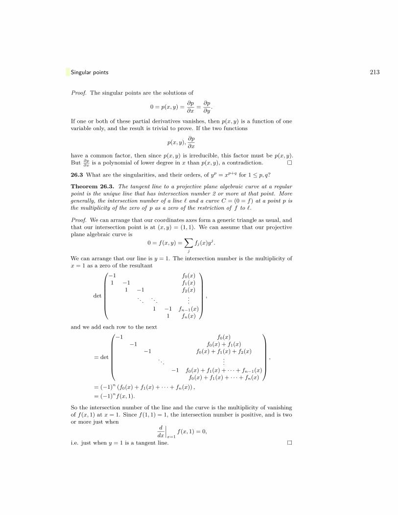
Singular points 213

Proof. The singular points are the solutions of

0 = p(x, y) = ∂p

∂x= ∂p

∂y.

If one or both of these partial derivatives vanishes, then p(x, y) is a function of onevariable only, and the result is trivial to prove. If the two functions

p(x, y), ∂p∂x

have a common factor, then since p(x, y) is irreducible, this factor must be p(x, y).But ∂p

∂xis a polynomial of lower degree in x than p(x, y), a contradiction.

26.3 What are the singularities, and their orders, of yp = xp+q for 1 ≤ p, q?

Theorem 26.3. The tangent line to a projective plane algebraic curve at a regularpoint is the unique line that has intersection number 2 or more at that point. Moregenerally, the intersection number of a line ` and a curve C = (0 = f) at a point p isthe multiplicity of the zero of p as a zero of the restriction of f to `.

Proof. We can arrange that our coordinates axes form a generic triangle as usual, andthat our intersection point is at (x, y) = (1, 1). We can assume that our projectiveplane algebraic curve is

0 = f(x, y) =∑j

fj(x)yj .

We can arrange that our line is y = 1. The intersection number is the multiplicity ofx = 1 as a zero of the resultant

det

−1 f0(x)1 −1 f1(x)

1 −1 f2(x). . . . . .

...1 −1 fn−1(x)

1 fn(x)

,

and we add each row to the next

= det

−1 f0(x)−1 f0(x) + f1(x)

−1 f0(x) + f1(x) + f2(x). . .

...−1 f0(x) + f1(x) + · · ·+ fn−1(x)

f0(x) + f1(x) + · · ·+ fn(x)

,

= (−1)n (f0(x) + f1(x) + · · ·+ fn(x)) ,= (−1)nf(x, 1).

So the intersection number of the line and the curve is the multiplicity of vanishingof f(x, 1) at x = 1. Since f(1, 1) = 1, the intersection number is positive, and is twoor more just when

d

dx

∣∣∣x=1

f(x, 1) = 0,

i.e. just when y = 1 is a tangent line.

214 The tangent line

Theorem 26.4. Denote by Cp the order of a projective algebraic plane curve C at apoint p. Then for any point p and projective algebraic plane curves C,D:

CpDp ≤ CDp,

with equality just when no line defined over any extension field is tangent to bothcurves at p.

Proof. If C or D is a line, our result is precisely theorem 26.3 on the preceding page.If either C or D is reducible, our result follows from induction on the degrees of thecomponents and adding up multiplicities.

After perhaps replacing our field by a finite degree extension, pick a generic trianglefor the two curves, and arrange that its vertices are (0, 0), (∞, 0), (0,∞) as usual. It iseasier to compute tangent lines if we shift the axes by adding constants to x and y toarrange that the vertices are at (−1,−1), (∞,−1), (−1,∞). We can then arrange thatour point p is (x, y) = (0, 0). Write the equations of our curves as C = (f = 0) andD = (g = 0). Then CDp is the order of x = 0 as a zero of the resultant r(x) = resf,g(x)in y. Let r ..= Cp, s ..= Dp. The lowest order homogeneous polynomial terms haveorder equal to the order of the point on the curve, so we can write out

f(x, y) = f0(x)xr + f1(x)xr−1y + · · ·+ fr(x)yr

+ fr+1(x)yr+1 + · · ·+ fm(x)ym,g(x, y) = g0(x)xs + g1(x)xs−1y + · · ·+ gs(x)ys

+ gs+1(x)ys+1 + · · ·+ gn(x)yn.

The tangent lines are the zero lines of the homogeneous terms of lowest order in x, y:

0 = f0(0)xr + f1(0)xr−1y + · · ·+ fr(0)yr,0 = g0(0)xs + g1(0)xs−1y + · · ·+ gs(0)ys.

We can assume that our axes are chosen so that the horizontal and vertical axes arenot tangent to either curve at the origin, i.e. to arrange that neither of these equationsare satisfied by (x, y) = (1, 0) or by (x, y) = (0, 1), i.e. none of

f0(0), g0(0), fr(0), gs(0)

vanishes. Since these tangent line equations are homogeneous, to find tangent lineswe can restrict to y = 1:

0 = f0(0)xr + f1(0)xr−1 + · · ·+ fr(0),0 = g0(0)xs + g1(0)xs−1 + · · ·+ gs(0).

The resultant of these two polynomials doesn’t vanish just when these polynomialshave no common factor, i.e. just when the curves C and D have no common tangentline; called this resultant R1.

The point (x, y) = (0, 0) is by assumption an intersection point of C and D. Wecan arrange, making our triangle generic enough, again perhaps using a field extension,that the lines x = 0 and y = 0 do not contain any other intersection points of C and

Singular points 215

D other than (x, y) = (0, 0). This is precisely saying that our polynomials

f(x, y) = f0(x)xr + f1(x)xr−1y + · · ·+ fr(x)yr

+ fr+1(x)yr+1 + · · ·+ fm(x)ym,g(x, y) = g0(x)xs + g1(x)xs−1y + · · ·+ gs(x)ys

+ gs+1(x)ys+1 + · · ·+ gn(x)yn.

do not both vanish when we substitute x = 0, except at y = 0, and vice versa.Plugging in x = 0:

f(0, y) = fr(0)yr + fr+1(0)yr+1 + · · ·+ fm(0)ym,g(0, y) = gs(0)ys + gs+1(0)ys+1 + · · ·+ gn(0)yn.

Dividing out common factors of y:

f(0, y)yr

= fr(0) + fr+1(0)y + · · ·+ fm(0)ym−r,

g(0, y)ys

= gs(0) + gs+1(0)y + · · ·+ gn(0)yn−s.

These are both polynomials and don’t vanish at y = 0, since f and g vanish exactlyto orders r and s at y = 0. These two polynomials also can’t both vanish anywhereelse, since there are no common roots of f and g on x = 0 except at y = 0. Hence theresultant of these two doesn’t vanish; call this resultant R2.

We next claim that resf,g(x) = xrsR1R2 + . . . has lowest order term given by thesetwo resultants. Before we prove our claim, note that if our claim is true, then CDp isgiven by the order of this resultant, so is at least rs, proving the theorem. Moreoverthis order is rs just when R1 6= 0 (since we know that R2 6= 0), i.e. just when thereare no common tangent lines.

We are left to justify this claim, i.e. to compute out the lowest order term of

resf,g(x) = det

f0(x)xr g0(x)xs

f1(x)xr−1 . . . g1(x)xs−1 . . ....

. . ....

. . .

fm(x). . . gn(x)

. . .

0. . . 0

. . .

.

The lowest order term in x is the same as the lowest order term of what happenswhen we plug x = 0 in all of the polynomials:

det

f0(0)xr g0(0)xs

f1(0)xr−1 . . . g1(0)xs−1 . . ....

. . ....

. . .

fm(0). . . gn(0)

. . .

0. . . 0

. . .

.

216 The tangent line

So it suffices to prove our result for the special case that all fj(x) and gj(x) areconstants, say:

f(x, y) = a0xr + a1x

r−1y + · · ·+ aryr

+ ar+1yr+1 + · · ·+ amy

m,

g(x, y) = b0xs + b1x

s−1y + · · ·+ bsys

+ bs+1ys+1 + · · ·+ bny

n.

Then the resultant is

resf,g(x) = det

a0xr b0x

s

a1xr−1 . . . b1x

s−1 . . ....

. . ....

. . .

am. . . bn

. . .

0. . . 0

. . .

.

We need to prove that this is xrsR1R2 + . . .. Write out

R1 = det

a0 b0

a1. . . b1

. . ....

. . ....

. . .

ar. . . bs

. . .

0. . . 0

. . .

and

R2 = det

ar bs

ar+1. . . bs+1

. . ....

. . ....

. . .

am. . . bn

. . .

0. . . 0

. . .

.

Let’s try a simple case: if r = 2, s = 1,m = 3, n = 2, the resultant is

resf,g(x) = det

a0x

2 0 b0x 0 0a1x a0x

2 b1 b0x 0a2 a1x b2 b1 b0xa3 a2 0 b2 b10 a3 0 0 b2

.

Sadly, when we expand out this determinant, we get a huge mess:

resf,g(x) = x2R1R2

+ x3(a23b

30 − 2 a1a3b

20b2 + 3 a0a3b0b1b2 + a2

1b0b22 − 2 a0a2b0b

22 − a0a1b1b

22)

+ x4a20b

32

Singular points 217

whereR1 = a2b

20 − a1b0b1 + a0b

21

andR2 = a2b2 − a3b1.

Nevertheless, the lowest term (as expected) is resf,g(x) = x2R1R2 + . . ..Returning to the general problem: luckily, we don’t really need to compute any of

these resultants at all. Suppose that r ≤ s. After rescaling f , x and y we can assumethat ar = 1 and that am = 1. Every term in g − bsxs−rf contains a factor of y, sowrite it as g − bsxs−rf = yg. We will see that replacing g by g, the three resultantswe have to calculate then all compute the same values. By problem 11.4 on page 83:

resf(x,y),g(x,y)(x) = resf(x,y),yg(x,y)(x),= resf(x,y),y(x) resf(x,y),g(x,y)(x),= f(x, 0) resf(x,y),g(x,y)(x),= xr resf(x,y),g(x,y)(x)

while, if we let F be the lowest order part of f , G the lowest order part of g, and Gthe lowest order part of g,

R1 = resF (x,1),G(x,1) = resF (x,1),G(x,1)

andR2 = res f(0,y)

yr ,yg(0,y)

ys= res f(0,y)

yr ,g(0,y)ys−1

.

Hence our claim is true for f, g just when it is true for f, g. Similarly, if r < s, swapthe roles of f and g and repeat. Apply induction on r and s, driving at least one ofthem to become smaller at each step, with the other staying the same. The inductionstops when one of them is zero, and C and D cease to intersect at p.

Chapter 27

Inflection points

Traditionally, an inflection point meant a point where the graph of a function changesfrom being convex down to being convex up, or vice versa. Clearly at any inflectionpoint, the derivative goes from decreasing to increasing, or vice versa, so the secondderivative vanishes. Notions of convexity depend very strongly on having some idea ofpositive and negative numbers, so they don’t apply in the context of algebraic curves.The closest we can come to this is to define an inflection point or flex of an algebraicplane curve to be a point at which the tangent line meets the curve to order 3 ormore.

To find such points, we define the Hessian det b′′(x, y, z) of a homogeneous poly-nomial b(x, y, z) by

det b′′(x, y, z) = det

(bxx bxy bxzbxy byy byzbxz byz bzz

)

where

bxy ..= ∂2b

∂x ∂y

and so on. So if b(x, y, z) is homogeneous of degree n, then bxy is homogeneous ofdegree n − 2, so det b′′(x, y, z) is homogeneous of degree 3(n − 2). If b(x, y, z) hasdegree 2, so that the associated curve is a conic, then det b′′(x, y, z) is a constant, thedeterminant of the symmetric matrix of coefficients of b(x, y, z). So det b′′(x, y, z) isa nonzero constant, i.e. H is empty, just when b(x, y, z) is a smooth conic. Similarly,det b′′(x, y, z) vanishes everywhere for a line or a singular conic (a pair of lines).

If the Hessian is not constant, the Hessian curve of the curve B = (0 = b(x, y, z))is the curve H = (0 = det b′′(x, y, z)).

Sage can compute Hessians for us:

P.<x,y,z> = PolynomialRing(QQ)b = x^3-y^2*z+z^3Hb = matrix([[diff(b,x,x),diff(b,x,y),diff(b,x,z)],

[diff(b,x,y),diff(b,y,y),diff(b,y,z)],[diff(b,x,z),diff(b,y,z),diff(b,z,z)]])

factor(Hb.det())

yields (−24) · x · (y2 + 3z2).

Working over any field of characteristic 3, the polynomial b(x, y, z) ..= x3 + y3 − z3

has derivatives 0 = bx = by = bz, and so has Hessian det b′′(x, y, z) = 0.

219

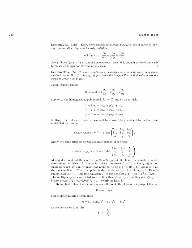
220 Inflection points

Lemma 27.1 (Euler). Every homogeneous polynomial b(x, y, z), say of degree n, overany commutative ring with identity, satisfies

nb(x, y, z) = x∂b

∂x+ y

∂b

∂y+ z

∂b

∂z.

Proof. Since b(x, y, z) is a sum of homogeneous terms, it is enough to check one suchterm, which is easy for the reader to check.

Lemma 27.2. The Hessian det b′′(x, y, z) vanishes at a smooth point of a planealgebraic curve B = (0 = b(x, y, z)) just when the tangent line at that point meets thecurve to order 3 or more.

Proof. Euler’s lemma:

nb(x, y, z) = x∂b

∂x+ y

∂b

∂y+ z

∂b

∂z

applies to the homogeneous polynomials bx ..= ∂b∂x

and so on to yield

(n− 1)bx = xbxx + ybxy + zbxz,

(n− 1)by = xbxy + ybyy + zbyz,

(n− 1)bz = xbxz + ybyz + zbzz.

Multiply row 1 of the Hessian determinant by x, row 2 by y, and add to the third rowmultiplied by z to get

z det b′′(x, y, z) = (n− 1) det

(bxx bxy bxzbxy byy byzbx by bz

).

Apply the same trick across the columns instead of the rows:

z2 det b′′(x, y, z) = (n− 1)2 det

bxx bxy bxbxy byy bybx by

nbn−1

.

At singular points of the curve B = (0 = b(x, y, z)), the final row vanishes, so thedeterminant vanishes. At any point where the curve B = (0 = b(x, y, z)) is notsingular, which we can arrange that point to be (x, y, z) = (0, 0, 1). Arrange thatthe tangent line of B at that point is the x-axis, so by = 1 while bx = 0. Euler’slemma gives bz = 0. Plug into equation 27 to get det b′′(0, 0, 1) = (n− 1)2bxx(0, 0, 1).The multiplicity of b restricted to x = 0 is then given by expanding out b(0, y) =b(0, 0) + by(0, 0)y + byy(0, 0)y2/2 + . . ., clearly at least 3.

By implicit differentiation, at any smooth point, the slope of the tangent line is

0 = bx + byy′

and so differentiating again gives

0 = bxx + 2bxyy′ + byy(y′)2 + byy′′,

as the derivative of y′. Soy′ = − bx

by,

Inflection points 221

whiley′′ = − bxx + 2bxyy′ + byy(y′)2

by.

Expanding out,

y′′ =−bxxb2y + 2bxybxby − byyb2x

b3y,

= 1b3y

(bxx bxy bxbxy byy bybx by 0

)

So at any point where b = 0, this is

y′′ = det b′′(x, y, 1)(n− 1)2b3y

.

If we take a point (x0, y0) at which by 6= 0, let y′0 be y′ at that point, and computeout that on the tangent line,

b(x, y) = b(x0 +∆x, y0 + y′0∆x),= b(x0, y0) + bx(x0, y0)∆x+ . . . ,

= −by(x0, y0)y′0∆x− by(x0, y0)y′′0∆x

2 + . . .

So the Hessian vanishes just where the tangent line meets the curve to order 3 ormore, and this occurs just where y′′ = 0.

Lemma 27.3. Take a plane algebraic curve B = (0 = b(x, y, z)). Suppose thatthe characteristic of the field is coprime to the exponents appearing in all terms ofb(x, y, z). Then b(x, y, z) has vanishing Hessian just when B is a union of lines. Inother words, B has Hessian curve H defined just when B is not a union of lines.

Proof. Continuing the previous proof, if we suppose that the Hessian vanishes ev-erywhere, we see that y′′ is everywhere zero, i.e. we see that at every point whereb = 0,

0 = y′′ = (y′)x + (y′)yy′.Plug in y′ = −bx/by to get (

bxby

)x

=(bxby

)(bxby

)y

.

This last equation turns a derivative in x into a product, with the first factor havingno derivative in x. Note that it only holds at points of the curve, so holds modulob. Hence, when we differentiate both sides, the result hold modulo b, bx, and so on.By induction, at a point where 0 = b = bx and where 0 6= by, if we differentiate bothsides repeatedly, we find a higher order x derivative of b vanishing each time. Soat any point where 0 = b = bx we also have 0 = b = bx = bxx = . . .. Because theexponents arising in the terms of b(x, y, z) are coprime to the characteristic of thefield, the vanishing of derivatives bx, bxx, . . . implies that the coefficients of x, x2, . . .in b(x, y, 1) are zero. Every term in b contains a factor of y, so b = 0 along the liney = 0.

222 Inflection points

Lemma 27.4. Take a plane algebraic curve B = (0 = b(x, y, z)), which has Hessiancurve H. Then H passes through all singular points of B, intersecting B at 3n(n−2)points at most, counting with multiplicity. The curves H and B meet at finitely manypoints. Moreover, H meets B at a smooth point of B with multiplicity r just whenthe tangent line at that point meets B with multiplicity r + 2.

Proof. We can assume that the point in question is the origin in the affine plane, andthat the tangent line is y = 0. Factoring out all copies of x from the terms with no yin them, the equation of B is now

0 = b(x, y) = y f(x, y) + xr+2g(x),

with f(0, 0) 6= 0 and g(0) 6= 0. We can rescale x, y to arrange f(0, 0) = 1 and g(0) = 1.The associated homogeneous polynomial is

b(x, y, z) = y f(x, y, z) + xr+2g(x, z).

Note that the affine equations f(0, 0) = 1 and g(0) = 1 become homogeneous equationsf(0, 0, z) = zn−1 and g(0, z) = zn−r−2. The Hessian det b′′(x, y, z) is extremelycomplicated in terms of f, g. The first derivatives are

bx = yfx + (r + 2)xr+1g + xr+2gx,

by = f + yfy + xr+2gy,

bz = yfz + xr+2gz,

and the second derivatives are

bxx = yfxx + (r + 2)(r + 1)xrg + 2(r + 2)xr+1gx + xr+2gxx,

bxy = fx + yfxy + (r + 2)xr+1gy + xr+2gxy,

bxz = yfxz + (r + 2)xr+1gz + xr+2gxz,

byy = 2fy + yfyy + xr+2gyy,

byz = fz + yfyz + xr+2gyz,

bzz = yfzz + xr+2gzz.

Modulo y, xr, i.e. dropping terms with y or xr in them, we find

det b′′(x, y, z) = det

( 0 fx 0fx 2fy fz0 fz 0

)= 0.

So every term in det b′′(x, y, z) contains either y or xr:

det b′′(x, y, z) = yF (x, y, z) + xrG(x, y, z)

for some polynomials F,G. We can absorb any y terms in G into F , so

det b′′(x, y, z) = yF (x, y, z) + xrG(x, z)

for some polynomials F,G. Compute det b′′(x, y, z) modulo y, and divide out xr fromthe first row, and then set x = 0, to find

G(0, 1) = det b′′

xr(0, 0, 1) = −(r + 2)(r + 1)g (0, 1) fz (0, 0, 1)2 .

We can actually get sage to compute this for us:

Inflection points 223

y=var(’y’)z=var(’z’)r=var(’r’)f = function(’f’)(x,y,z)g = function(’g’)(x,z)b(x,y,z) = y * f(x,y,z) + x^(r+2)*g(x,z)m=matrix([

[diff(b(x,y,z),x,x),diff(b(x,y,z),x,y),diff(b(x,y,z),x,z)],[diff(b(x,y,z),x,y),diff(b(x,y,z),y,y),diff(b(x,y,z),y,z)],[diff(b(x,y,z),x,z),diff(b(x,y,z),y,z),diff(b(x,y,z),z,z)]])

h=m.det()factor(simplify(expand((h.subs(y=0)/x^r).subs(x=0))))

prints out −(r + 2)(r + 1)g (0, z) D2 (f) (0, 0, z)2. (The sage notation for derivativesis peculiar, and we leave the reader to work out why D2 means derivative in the thirdvariable.) Since we know that f(0, 0, z) = zn−1 and g(0, 0, 1) = 1, we can computeout

G(0, 1) = det b′′

xr(0, 0, 1) = −(r + 2)(r + 1)(n− 1)2.

Returning to affine coordinates, at the origin (x, y) = (0, 0) in the (x, y) affine plane,

G(0) = −(r + 2)(r + 1)(n− 1)2 6= 0.

We are looking for H ∩B near the origin (0, 0, 1), i.e. we are looking for commonzeroes, with multiplicity, of

0 = yf(x, y, z) + xr+2g(x, z),0 = yF (x, y, z) + xrG(x, z).

Dehomogenize by setting z = 1:

0 = yf(x, y) + xr+2g(x),0 = yF (x, y) + xrG(x).

If r = 0, then the second equation doesn’t vanish near (x, y) = (0, 0), so the origin isnot an intersection point, contradicting our assumptions. So r ≥ 1.

Suppose that B and H share a common component, and suppose that the originbelongs to that component. If y = 0 on some intersection point, then plug in to getthat either x = 0 or g(x) = 0. But g(0) = 1, so g(x) is zero at only finitely manypoints, none near the origin. The same holds over any algebraic extension of our field.So (y = 0) is not a component of B ∩H, i.e. if B ∩H contains a curve, it is not insidethe line (y = 0). Solve for xr as

xr = y

(r + 1)(r + 2)(1 + . . . ) ,

and plug in to getx2y

(r + 1)(r + 2)(1 + . . . ) = −y 1 + . . .

1 + . . ..

Cancel the y, since (y = 0) is not in B ∩H:

x2 = −(r + 1)(r + 2)1 + . . .

1 + . . .,

224 Inflection points

and clear denominators:

x2(1 + . . . ) = −(r + 1)(r + 2)(1 + . . . ).

on any common component of B and H. But this is not satisfied at the origin, sothe common component does not meet the origin. Recall that we picked any point ofH ∩B and made it the origin. Hence B and H share no common component.

We will compute the multiplicity of intersection BHp at any smooth point p of B.We can assume that we have chosen very generic affine coordinates, so that the linethrough any two intersection points of B and H does not touch (0, 1) (even after analgebraic extension of the field). We can still arrange that p is the origin (0, 0) and thatthe tangent line to B at (0, 0) is y = 0. Take the resultant R(x) of yf(x, y) +xr+2g(x)and yF (x, y) + xrG(x). By theorem 23.6 on page 189, BHp is the order of vanishingof R(x) at the origin: if we write

f(x, y) =∑

yjfj(x),

F (x, y) =∑

yjFj(x),

then

R(x) = det

xr+2g(x) xrG(x)f1(x) xr+2g(x) F1(x) xrG(x)

... f1(x). . .

... F1(x). . .

fk(x). . . . . . xr+2g(x) F`(x)

. . . . . . xrG(x)

fk(x). . . f1(x) F`(x)

. . . F1(x). . .

.... . .

...fk(x) F`(x)

.

Expand across the top row to see that R(x) is a multiple of xr. We want to prove thatR(x) has order exactly xr, no something higher. The xr term in R(x) doesn’t noticeterms of order xr+1 or higher, so we can assume that g(x) and G(x) are constants,both equal to 1. Terms of higher order than xr make no contribution to the order rterm in R(x), so we only need to find the resultant of yf(x, y), yF (x, y) + xr. If wewrite dots to indicate terms of higher order than xr,

R(x) = resyf(x,y),yF (x,y)+xr + . . . ,

= resy,yF (x,y)+xr resf(x,y),yF (x,y)+xr + . . . ,

= xr resf(x,y),yF (x,y)+xr + . . . .

Suppose that the xr term vanishes. Then f(0, y) and yF (0, y) have a common root(in some algebraic extension), say y = y0. Then (0, y0) is a common root of yf(x, y) +xr+2g(x) and yF (x, y) + xrG(x), i.e. an intersection point (0, y0) ∈ B ∩ H. Thisintersection point is not at the origin, since f(0, 0) = 1. This intersection point is onthe line between (0, 1) and (0, 0), a contradiction. So the xr term in R(x) doesn’tvanish, i.e. the order of intersection BHp is r.

Corollary 27.5. A smooth plane algebraic curve of degree n with a defined Hessiancurve has exactly 3n(n−2) inflection points, counting multiplicities, in some algebraicextension field.

Inflection points 225

Proof. Follows from by Bézout’s theorem (theorem 23.7 on page 191) and the degreeof the Hessian being 3(n− 2) as above.

Chapter 28

Conics and quadratic forms

I like mathematics because it is not human and has nothing particularto do with this planet or with the whole accidental universe—because,like Spinoza’s god, it won’t love us in return.

— Bertrand Russell

Quadratic forms

A quadratic form is a homogeneous polynomial of degree 2.

Proposition 28.1 (Sylvester’s Law of Inertia). Every quadratic form in n variablesover the real numbers is identified, by some linear change of variables, with preciselyone of

x21 + x2

2 + · · ·+ x2p −(y2

1 + y22 + · · ·+ y2

q

)where p + q ≤ n. The triple of numbers (p, q, r) so that p + q + r = n is called thesignature of the quadratic form.

Proof. Write the quadratic form as

q(x) = a11x21 + a12x1x2 + · · ·+ annx

2n,

or in other words as q(x) = 〈Ax, x〉 for a symmetric matrix A. Apply an orthogonalchange of variables which diagonalizes the matrix A. Then rescale each variable toget the eigenvalues of the matrix to be ±1 or zero.

Lemma 28.2. Every quadratic form in n variables over a field k of characteristicnot 2 can be brought to the “diagonal” form

q(x) =∑

aix2i

by a linear change of variables. The ai are uniquely determined up to multiplying bysquares aib2i of nonzero elements bi of k.

Proof. Take a vector x for which q(x) 6= 0. Make a linear change of variables to getx = e1, so that q(e1) 6= 0. Hence after rescaling

q(x) = c1x21 + . . . ,

sayq(x) = c1x

21 + c2x1x2 + · · ·+ cnx1xn + . . .

227

228 Conics and quadratic forms

where x1 does not appear in the remaining terms. Replace x1, x2, . . . , xn withX1, x2, . . . , xn where

X1 ..= x1 −c22c1

x2 − · · · −cn2c1

x2

and check that nowq(x) = c1X

21 + . . .

where the . . . don’t involve X1, so we can apply induction.

For the real numbers, any positive real number has a square root, so we recover theprevious lemma.

For k = C, any complex number has a square root, so every quadratic form in ncomplex variables becomes

q(z) = z21 + z2

2 + · · ·+ z2p,

for a unique p ≤ q.

For k = Q, any rational number, up to multiplying by a nonzero square of a rationalnumber, is a square-free integer, i.e. has the form

α = ±p1p2 . . . ps

where all of the primesp1, p2, . . . , ps

are distinct. So every quadratic form over k has the form

q(x) =∑

αix2i

for square-free integers αi. In the associated conic curve, we can rescale the coef-ficients, so we can assume that the square-free integers αi have no common factor.We can also assume, by changing all signs if needed, that there are at least as manypositive αi as negative.

Since every element of any field obtains a square root in some extension, the quadraticforms over any algebraically closed field have the form

q(z) = z21 + z2

2 + · · ·+ z2p,

for a unique p ≤ q.

Theorem 28.3. Over a field k, take a quadratic form q, say in n variables. Thenafter perhaps repeatedly replacing k by a quadratic extension of k, finitely many times,and a linear change of variables, we can arrange that either

q(x1, . . . , xn) = x1x2 + x3x4 + x5x6 + · · ·+ xm−1xm

orq(x1, . . . , xn) = x2

1 + x2x3 + x4x5 + · · ·+ xm−1xm,

for some integer m.

Quadratic forms 229

Proof. A null vector of q is a vector v so that q(v + x) = q(x), i.e. translating q bya null vector doesn’t change the value of q. The null space of q is the set of all nullvectors. The null space is a linear subspace of kn since if v1 and v2 belong to the nullspace, then q(v1 + v2 + x) = q(v1 + x) = q(x) = q(v2 + x), and if v belongs to the nullspace, and c is any constant in k, then q(cv + x) = c2 q(v + x/c) = c2 q(x/c) = q(x).

Make a linear change of variables to get various of the variables to parameterizethis subspace, i.e. the subspace is given by setting the first j variables x1, x2, . . . , xjto zero and the last n− j variables xj+1, . . . , xn to any values. So q is a function ofthose first j variables only. We can reduce our problem to the study of those first jvariables, i.e. we can assume that the null space is zero.

If n = 1, q = ax2, we only need to ensure that a has a square root in k. If n = 2,q = ax2 + bxy + cy2, we only need to ensure that ax2 + bx+ c has a root in k, andthen q factors into linear factors, and we change variables to arrange that q = xy. Sosuppose that n ≥ 3.

A plane is a 2-dimensional linear subspace of kn. On any plane P , we can arrangethat q = 0 or q = x1x2 or q = x2

1, as above, after some linear change of variables. Forthe moment, suppose that there is a plane P on which we can arrange that q = x1x2,after perhaps a quadratic extension of k.

Consider the subset Q of kn consisting of those vectors w so that q(v + w) =q(v) + q(w) for all v in P . Expand out this equation to see that this is a linearequation in w, so Q is a linear subspace. Moreover, we only need to check theequation q(vi + w) = q(vi) + q(w) for any two vectors vi forming a basis of P , soQ is cut out by two linear equations, so has dimension at least n − 2. Check thatP ∩Q = { 0 }, because on P , q = x1x2. So Q is a linear subspace of kn of dimensionn− 2 exactly.

Make a linear change of variables so that P is spanned by the first two basisvectors (i.e. by setting any values to x1 and x2 while setting all remaining variablesequal to zero) and Q by the remaining n− 2 basis vectors: kn = P ⊕Q = k2 ⊕ kn−2.Change the first two variables if needed to arrange that q = x1x2 on P , as we saw ispossible. By induction, we can arrange that on Q, either

q(0, 0, x3, . . . , xn) = x3x4 + x5x6 + · · ·+ xn−1xn

orq(0, 0, x3, . . . , xn) = x3x4 + x5x6 + · · ·+ xn−2xn−1 + x2

n.

and soq(x1, . . . , xn) = x1x2 + x3x4 + x5x6 + · · ·+ xn−1xn

orq(x1, . . . , xn) = x1x2 + x3x4 + x5x6 + · · ·+ xn−2xn−1 + x2

n.

Now suppose that there is no plane P in kn on which we can arrange that qhas the form x1x2. Suppose that this remains true even after taking finitely manyquadratic extensions. So on any plane P in kn, either q = 0 or we can arrange thatq = x2

1.Let U be the set of all vectors in kn on which q vanishes. Take two linearly

independent vectors on which q vanishes, i.e. two points of U . On the plane theyspan, q vanishes on at least two lines, so q vanishes everywhere on that plane. So Uis a linear subspace of kn. Arrange by linear change of variables that U is given bythe linear equations 0 = xs+1 = · · · = xn. If s ≥ 2, then the plane parameterized by(x1, x2, 0, . . . , 0) intersects U only at the origin, i.e. q = 0 on that plane only at the

230 Conics and quadratic forms

origin. After a quadratic extension, as we have seen, we can arrange that q = x1x2,a contradiction. Hence s = 0 or s = 1. But s = 0 just when U = kn, i.e. just whenq = 0 everywhere. So we can assume that s = 1, i.e. 0 = q(0, x2, . . . , xn), i.e. q = 0whenever x1 = 0, i.e. q has a factor of x1, and so splits into a product of linearfactors.

Plane conics

Look at the curves x2 = y2 and the curves x2 + y2 = 0, defined over k = R; each is asingular plane conic. The first is a pair of lines x = ±y while the second, a circle ofradius zero, has the origin as its only real point, but splits into x = ±iy over k = C.

Lemma 28.4. If a plane conic over a field k has a singular point with coordinatesin k then it is either

a. a pair of lines defined over k or else

b. a pair of lines defined over a quadratic extension k(√α) meeting at a single point

defined over k, the singular point, and no other point of the curve is definedover k.

Proof. At a singular point of a plane conic, in an affine chart in which the singularpoint is the origin, the equation of the conic becomes a quadratic form in x, y. Thisfactors over k or over a quadratic extension of k, i.e. the conic is a pair of linesin a quadratic extension. If any point (except the origin) on one of those lines hascoordinates in k, then the line does, and so does the associated linear factor, and thenby dividing that linear factor in, we see that the other linear factor is also definedover k. Suppose on the other hand that the linear factors don’t exist over k, only overthe quadratic extension. Then no other point of the affine plane with coordinatesin k belongs to the curve, except the singular point. Write out the equation of thecurve as ax2 + bxy+ cy2 = 0, say. Switch to the affine chart y = 1 where the curve isax2 + bx+ c. Since the homogeneous equation has no roots in P1(k), this quadraticequation has no root in k, so there is no point in this affine chart y = 1. Thereforethe projective conic has precisely one point with coordinates in k.

Proposition 28.5. If a conic in the projective plane over a field k has a regular pointwith coordinates in k, it is either a pair of distinct lines, and taken to the conic xy = 0by some projective automorphism, or is irreducible and taken to the conic y = x2 bysome projective automorphism.

Proof. Suppose that our conic is not a pair of lines. It has a regular point withcoordinates in k, and is not a pair of lines, so it has no singular points, and so isirreducible. Arrange by projective automorphism that the regular point lies at theorigin of the affine chart z = 1 with tangent line y = 0, so the curve has the form

y = ax2 + bxy + cy2.

If a = 0, we get a factor of y on both sides, so the equation is reducible. Rescale y toarrange a = 1, and write the equation as x2 = y (1− bx− cy). Change variables by aprojective automorphism X = x, Y = y, Z = z − bx− cy to get to x2 = y.

Plane conics 231

Corollary 28.6. If an irreducible conic in the projective plane over a field k has aregular point with coordinates in k then it is birational to a line.

Proof. Suppose that the conic, call it C, has equation x2 = y, i.e. x2 = yz homoge-neously. Map

[s, t] ∈ P1(k) 7→[st, s2, t2

]∈ C ⊂ P2(k) .

The inverse map is

[x, y, z] ∈ C 7→{

[x, y], if y 6= 0,[z, y], if z 6= 0.

Clearly this identifies the rational functions.More geometrically, pick a regular point p0 on the curve, and arrange that it is

the origin in an affine chart. Then take a line ` in the plane, and identify each pointp ∈ ` of that line with the intersection point of the line pp0 with C. We leave thereader to check that this gives the same map.

Chapter 29

Projective duality

The set of lines in the projective plane P = P2(k) is called the dual plane and denotedP ∗ = P2∗(k). Each line has a homogeneous linear equation 0 = ax+ by + cz, uniqueup to rescaling, and so the point [a, b, c] is determined, allowing us to identify P ∗with P2(k) itself. The points of P ∗ correspond to lines in P . Through each point ofP , there is a pencil of lines; for example if the point is (x0, y0) in the affine chartz = 1, then the lines are a (x− x0)+ b (y − y0) = 0, or expanding out: ax+ by+ c = 0where c = −ax0 − by0. Hence in P ∗ the pencil is the line consisting of those points[a, b, c] so that ax0 + y0 + c = 0. So each point p of P is identified with a line p∗ inP ∗, consisting of those lines in P passing through p. Each line λ of P is identifiedwith a point λ∗ in P ∗. Given two points p, q of P and the line pq through them, thecorresponding lines p∗ and q∗ in P ∗ intersect at the point corresponding to (pq)∗. Wecan drop all of this notation and just say that each point p of P is a line in P ∗, andvice versa.

Dual curves

Take a projective algebraic curve C in P = P2(k) over a field k with algebraic closurek, with equation 0 = p(x, y) in some affine chart.

29.1 Denote partial derivatives as px ..= ∂p∂x

, etc. Show that at any point (x0, y0) ofC at which px 6= 0 or py 6= 0, the equation of the tangent line is

0 = px(x0, y0) (x− x0) + py(x0, y0) (y − y0) .

Lemma 29.1. In homogeneous coordinates [x, y, z] on P = P2, if the equation ofa curve C is 0 = p(x, y, z) with p(x, y, z) homogeneous, then the tangent line at apoint [x0, y0, z0] of C has homogeneous equation

0 = xpx(x0, y0, z0) + ypy(x0, y0, z0) + zpz(x0, y0, z0) .

Proof. Differentiate to get tangent line

0 = px(x0, y0, z0) (x− x0) + py(x0, y0, z0) (y − y0) + pz(x0, y0, z0) (z − z0) .

Take the equation that says that p(x, y, z) is homogeneous of degree d:

px(λx, λy, λz) = λdp(x, y, z),

and differentiate it in λ to get

xpx(λx, λy, λz) + ypy(λx, λy, λz) + zpz(λx, λy, λz) = dλd−1p(x, y, z).

Now set λ = 1 to getxpx + ypy + zpz = dp.

233

234 Projective duality

Plug into the homogeneous equation for the tangent line to get

0 = xpx(x0, y0, z0) + ypy(x0, y0, z0) + zpz(x0, y0, z0)− dp(x0, y0, z0) .

But at [x0, y0, z0] we know that p(x0, y0, z0) = 0.

Each line [a, b, c] in P ∗ has homogeneous equation ax+by+cz = 0, so the equationof the tangent line at each point [x0, y0, z0] of a curve with homogeneous equation0 = p(x, y, z) is [

abc

]=

[pxpypz

].

The dual curve of C is the smallest algebraic curve C∗ in P ∗ containing the tangentlines of C with coordinates in k.

Corollary 29.2. Every curve has a dual curve, i.e. the map[abc

]=

[pxpypz

]

taking the smooth points of C to P ∗ has image inside an algebraic curve.

Proof. Assume that the field is algebraically closed. Suppose that the image containsfinitely many points. The original curve has finitely many tangent lines, so is a finiteunion of lines. Following Study’s theorem (theorem 23.3 on page 186) we can assumethat C is irreducible, say C = (p(x, y, z) = 0). Take the four equations p = 0, a = px,b = py, c = pz, rescaling out any one of the x, y, z variables by homogeneity (or somelinear combination of them), and compute resultants for them in one of the x, y, zvariables, treating them as having coefficients rational in the other two x, y, z variablesand in a, b, c. Repeat until we get rid of x, y, z entirely. Since we have polynomialexpressions to begin with in all of our variables, each resultant is also polynomial inthose variables. By corollary 19.3 on page 160, perhaps making a linear change ofx, y, z variables before taking our first resultant, the resultants we end up are not allzero polynomials. So the image of the duality map lies in an algebraic curve in thedual plane. But the resultant vanishes just precisely on the points in the image of theduality map, since these equations specify precisely those points [a, b, c].

Chapter 30

Polynomial equations have solutions

For any field k, affine space kn is the set of all points

c =

c1c2...cn

with coordinates c1, c2, . . . , cn in k.

We want to say: if you have infinitely many polynomial equations, in a finite setof variables, you can throw away all but finitely many without changing the solutions.Let us be more precise. Recall that an ideal I in k[x] is a collection of polynomials sothat we can add and multiply polynomials in I without leaving I, and I is sticky: iff ∈ I and g ∈ k[x] then fg ∈ I. Any set S of polynomials generates an ideal (S): theideal is the set of all expressions

g1f1 + g2f2 + · · ·+ gsfs

where f1, f2, . . . , fs is any finite collection of polynomials in S and g1, g2, . . . , gs areany polynomials at all in k[x]. Given any set of polynomials, we can replace that setby the ideal of polynomials it generates inside k[x] without changing the roots of thepolynomials.

Theorem 30.1 (Hilbert basis theorem). For any field k and any variables x =(x1, x2, . . . , xn), every ideal I in k[x] is finitely generated. In other words, there arefinitely many polynomials

f1(x), f2(x), . . . , fs(x)in I so that the polynomials in I are precisely those of the form

g1(x)f1(x) + g2(x)f2(x) + · · ·+ gs(x)fs(x),

for any polynomials g1(x), g2(x), . . . , gs(x) in k[x].

Proof. The result is obvious if n = 0 since the only ideals in k are k and 0. Byinduction, suppose that the result is true for any number of variables less than orequal to n. Take an ideal I ⊂ k[x, y] where x = (x1, x2, . . . , xn) and y is a variable.Write each element f ∈ I as

f(x, y) = f0(x) + f1(x)y + · · ·+ fd(x)yd,

so that fd(x) is the leading coefficient. Let J be the set of all leading coefficients ofelements of I. Clearly J is an ideal in k[x], so finitely generated by induction. Sowe can pick polynomials f1(x, y), f2(x, y), . . . , fs(x, y) in I whose leading coefficientsgenerate the ideal J of all leading coefficients.

235

236 Polynomial equations have solutions

Let N be the maximum degree in y of any of the fj(x, y). Take some polynomialg(x, y) of degree greater than N in y, say with leading coefficient g(x). Express thatleading coefficient in terms of the leading coefficients fj(x) of the polynomials fj(x, y)as

g(x) =∑

hj(x)fj(x).

If we raise the y degree of fj(x, y) suitably to match the y degree of g(x, y), say bymultiplying by ykj , some positive integer kj , then∑

hj(x)ykjfj(x, y)

has leading coefficient the same as g(x, y), so

g(x, y) =∑

ykjhj(x)fj(x, y) + . . .

up to lower order in y. Inductively we can lower the order in y of g, replacing g by the. . ., until we get to order in y less than N . At each step, we modify g by somethingin the ideal generated by the fj(x, y).

Add to our list of fj(x, y) some additional fj(x, y) ∈ I to span all of the polynomialsin I of degree up to n. By induction we have generated all of the polynomials inI.

Theorem 30.2 (Nullstellensatz). Given a collection of polynomial equations in vari-ables

x = (x1, x2, . . . , xn) .

over a field k, either there is a point x = c defined in a finite algebraic extension fieldof k where all of these polynomials vanish or else the ideal generated by the polynomialsis all of k[x].

Proof. Follows from theorem 30.1 on the previous page and corollary 19.4 on page 161.

30.1 Given a point c ∈ kn, prove that the ideal

Ic ..= { f(x) | f(c) = 0 }

of functions vanishing at x = c is a maximal ideal. Prove that if x = p and x = q aredistinct points of kn, then Ip 6= Iq.

Corollary 30.3. Take variables

x = (x1, x2, . . . , xn) .

over an algebraically closed field k. Every maximal ideal in k[x] is the set of allpolynomial functions vanishing at some point c, for a unique point c.

Proof. Take any ideal I ⊂ k[x] Take a point c so that all polynomials in I vanishthere, using theorem 30.2. Then I ⊂ Ic.

Closed sets 237

Closed sets

An affine variety X = XS is the collection of zeroes of a set S of polynomials invariables

x = (x1, x2, . . . , xn) .A closed set in affine space kn (over a field k) is just another name for an affine variety.

The entire set kn is closed: it is the zero locus of the polynomial function p(x) = 0.

Every finite set in k is closed: the set { c1, c2, . . . , cn } is the zero locus of

p(x) = (x− c1) (x− c2) . . . (x− cn) .

Any infinite subset of k, except perhaps k itself, is not closed. We know that everyideal I in k[x] is generated by a single polynomial (the greatest common divisor ofthe polynomials in I), say I = p(x), so the associated closed set is the finite set ofroots of p(x).

A subset of k2 is closed just when it is either (a) all of k2 or (b) a finite union ofalgebraic curves and points.

An open set is the complement of a closed set. An open set containing a pointc of kn is a neighborhood of c. The intersection of any collection of closed sets is aclosed set: just put together all of the equations of each set into one set of equations.In particular, the intersection of all closed sets containing some collection X of pointsof kn is a closed set, the closure of X. A set S is dense in a closed set X if X is theclosure of S.

If the set X in kn is the zero locus of some polynomials fi(x) and the set Y in knis the zero locus of some polynomials gj(x), then X ∪ Y in kn is the zero locus of thepolynomials fi(x)gj(x). Hence the union of finitely many closed sets is closed.

30.2 Give an example of a field k and a polynomial b(x, y) over k so that the pointsin the image of the polynomial (i.e. the points of the form z = b(x, y) for any x andy in k) do not form an affine subvariety of k.

Chapter 31

More projective planes

So full of shapes is fancyThat it alone is high fantastical.

— William ShakespeareTwelfth Night

The pure mathematician, like the musician, is a free creator of his worldof ordered beauty

— Bertrand Russell

We know that man has the faculty of becoming completely absorbed in asubject however trivial it may be, and that there is no subject so trivialthat it will not grow to infinite proportions if one’s entire attention isdevoted to it.

— Leo TolstoyWar and Peace

Projective planes

A projective plane (in a more general sense of the term than we have used previously)is a set P , whose elements are called points, together with a set L, whose elementsare called lines, and a defined notion of incidence, i.e. of a point being “on” a line (orwe could say that a line is “on” or “through” a point) so that

a. Any two distinct points both lie on a unique line.b. Any two distinct lines both lie on a unique point.c. There are 4 points, with no 3 on the same line.

We usually denote a projective plane as P , leaving its set L of lines understood, andits notion of incidence understood.

Lemma 31.1. The projective plane P2(k) over any field is a projective plane in thismore general sense.

239

240 More projective planes

Proof. Given any two distinct points of P2(k), they arise from two distinct vectors ink3, determined up to rescaling. Such vectors lie in a basis of k3, and span a plane ink3 through the origin. The lines in that plane lying through the origin consitute aprojective line through the two points. Similarly, any two distinct projective lines arethe lines through the origin of two distinct planes through the origin. Those planes areeach cut out by a linear equation, and the linear equations have linearly independentcoefficients, because they are distinct planes. But then the simultaneous solutions ofthe two equations in three variables form a line through the origin, a projective point.To find 4 points, with no 3 on the same line, consider the 3 points[1

ab

],

[01c

],

[001

]

for any constants a, b, c from k. For these points to be on the same projective line,the corresponding vectors (1

ab

),

(01c

),

(001

)must lie on the same plane, i.e. satisfying the same linear equation with not allcoefficients zero. But these vectors are linearly independent. Now take the 4 points[1

10

],

[101

],

[010

],

[001

]

and check that any 3 do not lie in a projective line.

31.1 Prove that every line in a projective plane contains at least three points.

Duality

We defined polygons in projective planes over fields in section 24 on page 197; weemploy the same definitions in any projective plane. If P is a projective plane withset of lines L, the dual projective plane, denoted P ∗, has L as its set of “points” andP as its set of “lines”, and the same incidence notion, i.e. we use interchange thewords “point” and “line”.

Lemma 31.2. The dual P ∗ of a projective plane P is a projective plane, and P ∗∗ =P .

Proof. We have only to check that there is a quadrilateral in P ∗. Pick a quadrilateralin P , and we need to see that its 4 edges, in the obvious cyclic ordering, are thevertices of a quadrilateral in P ∗. Three of those vertices in P ∗ lie on a line in P ∗

just when three of the lines of the original quadrilateral lie through the same point,say p. So we need to prove that no quadrilateral has three of its edges through thesame point. Taking the remaining edge as the fourth edge, the first three edges of thequadrilateral pass through the same point, so that point is the first and the secondvertex. But then the third vertex lies on a line with the first two.

Projective spaces 241

For example, if V is a 3-dimensional vector space over a field k, the associatedprojective plane PV is the set of lines through the origin of V . A line in PV is aplane through the origin of V . Every plane through the origin is the set of solutionsof a linear equation, i.e. is the set of zeroes of a linear function f : V → k, i.e. of anelement 0 6= f ∈ V ∗ of the dual vector space. Such a function is uniquely determinedby its zeroes, up to rescaling. So each line in PV is identified with a 2-plane throughthe origin of V and thereby with a linear function f ∈ V ∗ defined up to rescaling, andthereby with a line k · f ⊂ V ∗ through the origin of V ∗, and thereby with a point ofPV ∗: P(V ∗) = P(V )∗.

Projective spaces

A projective space is a pair of sets, called the sets of points and lines, together with adefinition of incidence of points on lines, so that

a. Any two distinct points p, q are on exactly one line pq.b. Every line contains at least three points.c. For any four points p, q, r, s, with no three on the same line, if pq intersects rs

then pr intersects qs.Points are collinear if they lie on a line, and lines intersect at a point if they both lieon that point. By a. and b., every line of a projective space is determined uniquelyby the set of points lying on it. Therefore it is safe to think of lines as sets of points.

31.2 Prove that Pn(k) is a projective space, for any field k.

Given a point p and a line `, let p`, the plane spanned by p and `, be the set ofpoints q so that q = p or pq intersects `. A line of a plane P = p` in a projectivespace is a line of the projective space which intersects two or more points of P .

Lemma 31.3. Every plane in a projective space is a projective plane.

Proof. Take a projective space S, and a plane P = p` in S. Looking at the definitionof projective space, the first requirement ensures the first requirement of a projectiveplane: any two distinct points line in a unique line. Take two distinct lines m,n. Weneed to show they intersect at a unique point, and that this point also lies in P .

First, suppose that m = ` and that p lies on n. We need to prove that n intersects`. By definition of lines in a plane, there are at least two points of P on each line ofP . Pick a point q 6= p from P on n. Then n = pq intersects m = ` at a point of `, bydefinition of a plane.

Next, suppose that m = ` but that p does not lie on n. We need to prove that nintersects `. By definition of n being a line on the plane P , n contains two points of P .Pick two points q, q′ of P lying on n. If either point lies on `, we are done. Let r, r′be the intersection points of pq, pq′ with `, which exist by definition of a plane. Thenpq = qr and pq′ = q′r′ so qr and q′r′ intersect at p. Suppose that three of q, q′, r, r′lie on the same line. But n = qq′ so that line is n. But then r is on n, so n intersects`, and we are done. So we can assume that q, q′, r, r′ are not collinear. By property c.,since qr and q′r′ intersect (at p), qq′ = n intersects rr′ = `.

Next, suppose that m 6= `. Repeating the above if n = `, we can assume thatn 6= `. From the above, m and n both intersect `, say at points a and b. If a = bthen m and n intersection and we are done. If a 6= b, take points a′ 6= a in m and

242 More projective planes

b′ 6= b in n both lying in P . Repeating the above, a′b′ intersects `. So either three ofa, a′, b, b′ are collinear, or aa′ = m intersects bb′ = n. Suppose that three of a, a′, b, b′are collinear. Then one of b or b′ lies in m, or one of a, a′ lies in n, so m and nintersect at a point of P . Therefore we can assume that no three of a, a′, b, b′ arecollinear. By property c. on the preceding page, since a′b′ and ab intersect, aa′ = mintersects bb′ = n. We have established that any two lines of P intersect in S. Wehave to prove that this intersection point c lies in the plane P . The line pa is a lineof P , and so intersects `, m and n. The line n = bc is also a line of P . If three ofp, a, b, c are collinear, then p lies in n or a lies in n, and we are done as above. Byproperty c. on the previous page, since pa and bc intersect, pc intersects ab = `. Bydefinition of a plane, the point c belongs to P . So we have established that any twodistinct lines of P lie on a unique point of P .

Finally, take two distinct points a, b on ` and a′ 6= a on pa and b′ 6= b on pb. Bydefinition, a, b, a′, b′ all lie on P . Collinearity of any three of these points would, bythe same argument, force a = b.

Corollary 31.4. If a line lies in a plane in a projective space, then every point lyingon that lie lies on that plane.

A projective subspace of a projective space of dimension −∞ means an empty set,of dimension zero means a point, and inductively of dimension n+ 1 means the unionof all points on all lines through a projective subspace of dimension n and a disjointpoint. A line of a projective subspace is a line of the projective space containing twoor more points of the subspace. Clearly every projective subspace is itself a projectivespace, by induction from the proof that every plane in a projective space is a projectiveplane.

Lemma 31.5. In any 3-dimensional projective space, every line meets every plane.

Proof. Pick a plane P . We want to see that every line ` meets P . Suppose that ` = abfor two points a, b. If either of a, b are on P , then ` meets P , so suppose otherwise.

Pick a point q0 not in P . Suppose that a 6= q0 and b 6= q0. Each of a, b lies ona line q0a′, q0b′, for some a′, b′ on P , since our projective space has dimension 3. Ifa = a′ then a is on P and ` so ` meets P . Similarly if b = b′. Therefore we cansuppose that a 6= a′ and b 6= b′. So aa′ and bb′ intersect at q0. Suppose that three ofa, a′, b, b′ lie on a line. Then aa′ = q0a

′ contains b or b′, so equals ab = ` or a′b′ lyingon P . In the first case, ab = ` then contains a′, which lies on P , so ` meets P . In thesecond case, a′b′ lies in P and contains a which lies on `, so ` meets P . So we canassume that no three of a, a′, b, b′ lie on a line. By c., ab intersects a′b′, so ` intersectsa line in P .

Lemma 31.6. Any two distinct planes in a 3-dimensional projective space meet alonga unique line.

Proof. Take planes P 6= P ′. Take a point p0 in P but not P ′. Pick two distinct lines`,m in P through p0. Let a be the intersection of ` and P ′, and b the intersection ofm and P ′. The line ab lies in P ′ and P . If some common point c of P and P ′ doesnot lie in ab, then the plane abc lies in P and P ′, so P = P ′.

The quaternionic projective spaces 243

The quaternionic projective spaces

The quaternions over a commutative ring R are the quadruples a = (a0, a1, a2, a3) ofelements of R, each written as

a = a0 + a1i+ a2j + a3k.

They form the ring HR with addition component by component and multiplicationgiven by the rules

i2 = j2 = k2 = −1, ij = k, jk = i, ki = j, ji = −k, kj = −i, ik = −j,

and conjugation defined by

a = a0 − a1i− a2j − a3k.

The quaternions H (with no underlying commutative ring specified) are the quater-nions over R = R.

31.3 Prove that HR is associative, by a direct computation.

A skew field is an associative ring with identity, not necessarily commutative, inwhich every element a has a multiplicative inverse: a−1a = aa−1 = 1.

31.4 Check thataa = aa = a2

0 + a21 + a2

2 + a23.

In particular, if k is a field in which sums of squares are never zero unless all elementsare zero (as when k = R), prove that Hk is a skew field.

31.5 Suppose that k is a skew field. Define P2(k) by analogy with the definition fora field. Explain why P2(k) is then a projective plane.

The quaternionic projective plane P2(H) is the projective plane of the quaternions.Take a skew field k. Add vectors x in kn as usual component by component, but

multiply by elements ra in k on the right:x1x2...xn

a =

x1ax2a...

xna

.

Multiply by matrices on the left as usual.A vector space V over a skew field k is a set V equipped with an operation u+ v

and an operationa va so thatAddition laws:

1. u+ v is in V2. (u+ v) + w = u+ (v + w)3. u+ v = v + u

for any vectors u, v, w in V ,Zero laws:

244 More projective planes

1. There is a vector 0 in V so that 0 + v = v for any vector v in V .2. For each vector v in V , there is a vector w in V , for which v + w = 0.

Multiplication laws:

1. va is in V2. v · 1 = v

3. v(ab) = (va)b4. v(a+ b)v = va+ vb

5. (u+ v)a = ua+ va

for any numbers a, b ∈ k, and any vectors u and v in V .For example, V = kn is a vector space, with obvious componentwise addition andscaling. A subspace of a vector space V is a nonempty subset U of V so that whenwe apply the same scaling and addition operations to elements of U we always getelements of U . In particular, U is also a vector space.

A linear relation between vectors v1, v2, . . . , vp ∈ V is an equation

0 = v1a1 + v2a2 + · · ·+ vpap

satisfied by these vectors, in which not all of the coefficients a1, a2, . . . , ap vanish.Vectors with no linear relation are linearly independent. A linear combination ofvectors v1, v2, . . . , vp ∈ V is vector

v1a1 + v2a2 + · · ·+ vpap

for some elements a1, a2, . . . , ap from k. One weird special case: we consider the vector0 in V to be a linear combination of an empty set of vectors. The span of a set ofvectors is the set of all of their linear combinations. A basis for V is a set of vectorsso that every vector in V is a unique linear combination of these vectors. Note thatsome vector spaces might not have any basis. Also, if V = { 0 } then the empty set isa basis of V .

Theorem 31.7. Any two bases of a vector space over a skew field have the samenumber of elements.

Proof. If V = { 0 }, the reader can check this special case and see that the empty setis the only basis. Take two bases u1, u2, . . . , up and v1, v2, . . . , vq for V . If needed,swap bases to arrange that p ≤ q. Write the vector v1 as a linear combination

v1 = u1a1 + u2a2 + · · ·+ upap.

If all of the elements a1, a2, . . . , ap vanish then v1 = 0, and then zero can be written asmore than one linear combination, a contradiction. By perhaps reordering our basisvectors, we can suppose that a1 6= 0. Solve for u1:

u1 = (v1 + u2 (−a2) + · · ·+ up (−ap)) a−11 .

We can write every basis vector u1, u2, . . . , up as a linear combination of v1, u2, . . . , up,and so the span of v1, u2, . . . , up is V . If there is more than one way to write a vectorin V as such a linear combination, say

v1b1 + u2b2 + · · ·+ upbp = v1c1 + u2c2 + · · ·+ upcp

Incidence geometries 245

then the difference between the left and right hand sides is a linear relation

0 = v1d1 + u2d2 + · · ·+ updp.

Solve for v1 in terms of u1 and plug in:

0 = u1a1d1 + u2 (d2 + a2d1) + · · ·+ up (dp + apd1) .

Since these u1, u2, . . . , up form a basis,

0 = a1d1 = d2 + a2d1 = · · · = dp + apd1.

Multiplying the first equation by a−11 gives d1 = 0, and then that gives 0 = d2 =

· · · = dp, a contradiction. Therefore v1, u2, . . . , up is a basis. By induction, repeatingthis process, we can get more and more of the vectors v1, v2, . . . , vq to replace thevectors u1, u2, . . . , up and still have a basis. Finally, we will find a basis u1, u2, . . . , upconsisting of a subset of p of the vectors v1, v2, . . . , vq. But then every vector is aunique linear combination of some subset of these vectors, a contradiction unless thatsubset is all of them, i.e. p = q.

The dimension of a vector space is the number of elements in a basis, or∞ if thereis no basis. A linear map f : V →W between vector spaces V,W over a skew field kis a map so that f(v1 + v2) = f(v1) + f(v2) for any v1, v2 in V and f(va) = f(v)a forany v in V and a in k.

31.6 Prove that for any linear map f : V → W between vector space V = kq andW = kp, there is a unique p× q matrix A with entries from k so that f(v) = Av forany v in V .

The kernel of a linear map f : V → W is the set of all vectors v in V so thatf(v) = 0. The image of a linear map f : V → W is the set of all vectors w in W ofthe form w = f(v) for some v in V .

31.7 Prove that the kernel and image of a linear map f : V →W are subspaces of Vand of W and that their dimensions add up to the dimension of V .

31.8 Prove that for any basis v1, v2, . . . , vn for a vector space V , there is a uniquelinear map f : V →W with has any given values f(vi) = wi.

31.9 Imitating the proof of lemma 31.1 on page 239, prove that P2(k) is a projectiveplane for any skew field k.

31.10 Prove that Pn(k) is a projective space for any skew field k.

Incidence geometries

We want to consider more general configurations of points and lines than projectiveplanes or spaces. An incidence geometry, also called a configuration, is set P , whoseelements are called points, together with a set L, whose elements are called lines, anda defined notion of incidence, i.e. of a point being “on” a line (or we could say that aline is “on” or “through” a point).

246 More projective planes

As points, take P ..= Z/mZ and as lines takes L ..= Z/mZ and then say that a pointp is on a line ` if p = ` or p = `+ 1. Call this a polygon or an m-gon. If m = 3, callit a triangle, and if m = 4 a quadrilateral.

Any projective plane or projective space is a configuration.

The affine plane is a configuration.

If we just draw any picture on a piece of paper of some dots (“points”) and somesquiggly curves (“lines”, not necessarily straight), with some indication which linesintersect which points, that describes a configuration. For example, we can draw theFano plane as:

55

33

66

11

77 22

4

where the “points” are the numbered vertices and the “lines” are the straight lines,including the three straight lines through the center, and the circle.

A morphism of configurations

f : (P0, L0)→ (P1, L1)

is a pair of maps, both called f , f : P0 → P1 and f : L0 → L1 so that if a point p lieson a line `, then f(p) lies on f(`).

Every projective plane contains a quadrilateral, so has a morphism from the quadri-lateral P = Z/4Z.

Take the Fano plane, using our diagram, and delete the one line corresponding to thecircle; call the result the kite. Every projective plane P2(k) over a field k contains thepoints [x, y, z] for x, y, z among 0, 1 and not all zero, and contains the various linesbetween them, i.e. contains the kite. So there is a morphism, injective on points andlines, from the kite to every projective plane over any field. In fact, if we start offwith any quadrilateral in any projective plane, and we draw from it all lines throughany two of its vertices, and then all of the intersections of those lines, and then alllines through any two vertices of that configuration, and so on, we end up with thekite.

If k has a field extension K, then the obvious map P2(k)→ P2(K) is a morphism.

An isomorphism is a morphism whose inverse is also a morphism, so that a pointlies on a line just exactly when the corresponding point lies on the correspondingline. An automorphism of a configuration is an isomorphism from the configurationto itself. A monomorphism is a morphism injective on points and on lines, so that apoint lies on a line after we apply the morphism just when it did before.

By definition, every projective plane admits a monomorphism from a quadrilateral.

Desargues’ theorem 247

The map P2(R)→ P2(C) is not an isomorphism, as it is not onto on either points orlines, so has no inverse, but it is a monomorphism.

The map f : Pn(k)→ Pn+1(k) taking

f [x0, x1, . . . , xn] = [x0, x1, . . . , xn, 0]

is a monomorphism.

Invertible matrices with entries in a field k act as projective automorphisms onP2(k), and similarly in all dimensions; call these linear projective automorphisms ork-projective automorphisms.

Let k ..= Q(√

2) and let f : k → k be the automorphism

f(a+ b

√2)

= a− b√

2

for any a, b in Q. Then clearly f extends to kn+1 for any integer n, and so extendsto Pn(k), giving an automorphism which is not linear.

31.11 Any two quadrilaterals in the projective plane P2(k) over any field k can betaken one to the other by a linear automorphism. Hint: think about the linear algebrain k3, get the first three vectors where you want them to go, and think about rescalingthem to get the last vector in place.

The dual of a configuration has as line the points and as points the lines and thesame incidence relation. If f : A → B is a morphism of configurations, define thedual morphism to be the same maps on points and lines, but interpreted as lines andpoints respectively.

Desargues’ theorem

Beauty is the first test: there is no permanent place in the world forugly mathematics

— G. H. Hardy

Two triangles with a chosen correspondence between their vertices are in perspec-tive from a point p if the lines through corresponding vertices pass through p.

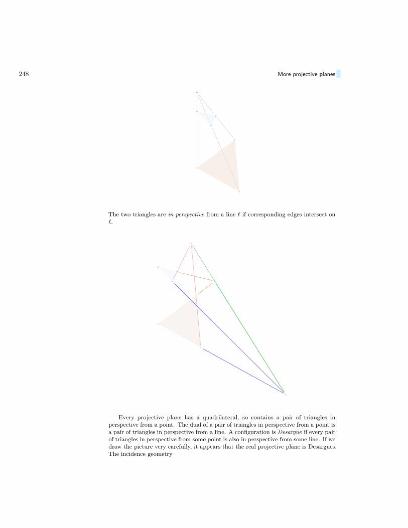
248 More projective planes

The two triangles are in perspective from a line ` if corresponding edges intersect on`.

Every projective plane has a quadrilateral, so contains a pair of triangles inperspective from a point. The dual of a pair of triangles in perspective from a point isa pair of triangles in perspective from a line. A configuration is Desargue if every pairof triangles in perspective from some point is also in perspective from some line. If wedraw the picture very carefully, it appears that the real projective plane is Desargues.The incidence geometry

Desargues’ theorem 249

is the standard Desargues configuration. The same configuration with three curvesadded through those 3 points to determine a triangle is the broken Desargues config-uration.

A configuration is thus Desargues just when every morphism to it from the configu-ration of a pair of triangles in perspective extends to a morphism from a standard

250 More projective planes

Desargue configuration, or equivalently the configuration admits no monomorphismsfrom the broken Desargues configuration. Not every projective plane is Desargues, aswe will see.

31.12 Prove that a projective plane is Desargues precisely when, for any pair oftriangles in perspective, their dual triangles in the dual projective plane are also inperspective.

Lemma 31.8. Every 3-dimensional projective space is Desargues.

Proof. Looking back at our drawings of triangles in perspective, suppose that the twotriangles lie on different planes. Then these two planes intersect along a single line.The lines drawn along the sides of either triangle lie in one or the other of those twodifferent planes, and intersect along that line. Therefore the intersection points lie onthat line, i.e. the intersection points are collinear.

But so far we have assumed that the two triangles in perspective lie in differentplanes. Suppose that they lie in the same plane. We want to “perturb” the trianglesout of that plane. Pick a point outside that plane, which exists by axiom c., and callit the perturbed origin o′. On the line o′a from the perturbed origin o′ to one of thevertices a of the first triangle, pick a point, the perturbed vertex a′ of the first triangle,not lying in the original plane. Take the vertex A in the second triangle correspondingto a. The points o, a,A are collinear by definition of triangles in perspective. Thepoints o, o′, a, A therefore are coplanar. The point a′ by construction lines in thisplane. So the lines oa′ and o′A lie in that plane, and intersect in a point A′, theperturbed vertex of the second triangle. The triangles with perturbed vertices arenow in perspective from the origin o (not from the perturbed origin). The perturbedtriangles lie in different planes, since otherwise the entire perturbed picture lies ina single plane, which contains the other vertices of our two triangles, so lies in theoriginal plane.

Essentially we just perturbed a vertex of the first triangle, and then suitablyperturbed the corresponding one in the second triangle to get a noncoplanar pair oftriangles in perspective. The intersection points p′, q′, r′ of the perturbed standardDesargues configuration lie in a line p′q′r′ by the previous reasoning. Take the planecontaining that line p′q′r′ and the perturbed origin o′. That plane intersects the planeP of the original unperturbed triangles along a line `. The lines o′p′, o′q′, o′r′ intersectthe plane P at the three intersection points p, q, r of the unperturbed configuration,so these lie in `.

Theorem 31.9. Every projective space of dimension 3 or more is Desargue.

Proof. Start with any triangle: it lies on a plane. Add one more point: the picturestill lies in a 3-dimensional projective space. But then we can start our sequenceof pictures above constructing the two triangles in perspective, and then the entireDesargues configuration, inside that 3-dimensional projective space.

For example, projective space Pn(k) of any dimension n ≥ 3 over any skew field kis Desargues.

Corollary 31.10. If a projective plane embeds into a projective space of some dimen-sion n ≥ 3, then the projective plane is Desargues.

For example, projective space Pn(k) of any dimension n ≥ 2 over any field k isDesargues.

Generating projective planes 251

Generating projective planes

A monomorphism A → P from a configuration to a projective plane P is universalif every monomorphism A→ Q to a projective plane Q factors through a morphismP → Q, i.e. A → P → Q. A configuration is planar if any two distinct points of Alie on at most one line. A planar configuration is spanning if there are 4 points withno three collinear.

Lemma 31.11. A configuration is planar if and only if it has a monomorphism to aprojective plane. A planar configuration is spanning if and only if it has a universalmonomorphism to a projective plane; this projective plane, the plane generated by theconfiguration, is then unique up to a unique isomorphism.

Proof. Note that any two lines of a planar configuration A intersect at, at most, onepoint, since otherwise they would contain two distinct points lying on two differentlines.

For any configuration B, let B+ have the same points as B, but add in a new linefor each pair of points that don’t lie on a line. To be more precise, we can let thelines of B+ be the lines of B together with the unordered pairs of points {p, q} of Bthat don’t lie on a line of B.

For any configuration B, let B+ have the same lines as B, but add in a new pointfor each pair of lines that don’t lie on a point. To be more precise, we can let thepoints of B+ be the points of B together with the unordered pairs of lines {m,n}of B that don’t lie on a point of B. Inductively, let A0 ..= A, A2j+1 ..= A2j,+ andA2j+2 ..= A+

2j+1.Let P be the configuration whose points are all points of A1, A2, . . ., and whose

lines are the lines of A1, A2, . . .. Clearly any two distinct points of P lie on a uniqueline, and any two distinct lines of P lie on a unique point. Suppose that A is spanning.Three noncollinear points of A will remain noncollinear in A+, because we only addnew points. They will also remain noncollinear in A+, because we only add new linesthrough pairs of points, not through triples. Therefore they remain noncollinear inP , so that P is a projective plane.

If f : A → Q is a monomorphism to a projective plane, define f : A+ → Q byf {p, q} = f(p)f(q), and similarly for A+ → Q, to define a morphism f : P → Q.

Given another universal morphism f ′ : A→ P ′, both monomorphisms must factorvia A→ P → P ′ and A→ P ′ → P . These factoring maps P → P ′ and P ′ → P areisomorphisms, as one easily checks, by looking step by step at how they act on pointsand lines.

A trivalent configuration is one in which every point is on at least three lines andevery line is on at least three points.

Lemma 31.12. Take a spanning planar configuration A and its universal morphismto a projective plane A → P . Every monomorphism T → P from a finite trivalentconfiguration factors through T → A→ P .

Proof. At each stage of constructing P , we never put in a new line passing throughmore than two points. So among the lines of T , the last to appear in the constructionof P contains only two points, a contradiction, unless T lies in A.

252 More projective planes

Let A have 4 points and no lines, like ::, which is clearly spanning and planar. TakeP to be the projective plane generated by A. By the lemma, no line in P contains 3points. As every line in the Desargues configuration contains 3 points, P does notcontain the Desargues configuration. Start with the quadrilateral given by the pointsof A, thought of as one point and one triangle of P . Since every line in any projectiveplane contains at least 3 points, we can then build a pair of triangles in perspectivein P out of our triangle and point, as in our pictures of the Desargues configuration.Therefore P is not Desargues.

Octonions

In this section, we will allow the use of the word ring in a somewhat more generalcontext. A ring is a set of objects S together with two operations called addition andmultiplication, and denoted by b+ c and bc, so that if b and c belong to S, then b+ cand bc also belong to S, and so that:

Addition laws:

a. The associative law: For any elements a, b, c in S: (a+ b) + c = a+ (b+ c).b. The identity law: There is an element 0 in S so that for any element a in

S, a+ 0 = a.c. The existence of negatives: for any element a in S, there is an element b

in S (denote by the symbol −a) so that a+ b = 0.d. The commutative law: For any elements a, b in S, a+ b = b+ a.

Multiplication laws:The Distributive Law:

a. For any elements a, b, c in S: a(b+ c) = ab+ ac.

We do not require the associative law for multiplication; if it is satisfied the ring isassociative.

A ring is a ring with identity if it satisfies the identity law: There is an element1 in S so that for any element a in S, a1 = a. We will only ever consider rings withidentity.

A ring is a division ring if it satisfies the zero divisors law: for any elements a, bof S, if ab = 0 then a = 0 or b = 0.

A ring is commutative if it satisfies the commutative law: for any elements a, b ofS, ab = ba.

The associative law for addition, applied twice, shows that (a + b) + (c + d) =a+ (b+ (c+ d)), and so on, so that we can add up any finite sequence, in any order,and get the same result, which we write in this case as a+ b+ c+ d. A similar storyholds for multiplication if R is associative.

Any skew field k has a projective space Pn(k) for any integer n, defined as the setof tuples

x = (x0, x1, . . . , xn)with x0, x1, . . . , xn ∈ k, but with two such tuples equivalent just when the secondequals the first scaled by a nonzero element:

x = (x0, x1, . . . , xn) ∼= xc = (x0c, x1c, . . . , xnc) .

Octonions 253

This approach doesn’t work for nonassociative rings, because it might be that (xa)bcan not be written as x(ab) or even as xc for any c. It turns out to be a very trickyproblem to define a meaning for the expression Pn(R) if R is a nonassociative ring, aproblem which does not have a general solution.

A conjugation on a ring R is a map taking each elements b of R to an element,denoted b, of R, so that

a. b+ c = b+ c,b. bc = cb,c. 1 = 1 if R has a chosen multiplicative identity element 1,

d. b = b,for any elements b, c of R. A ring with a conjugation is a ∗-ring. If R is a ∗-ring, letR+ be the set of pairs (a, b) for a, b in R; write such a pair as a+ ιb, and write a+ ι0as a, so that R ⊂ R+. Endow R+ with multiplication

(a+ ιb) (c+ ιd) ..= ac− db+ ι (ad+ cb)

with conjugationa+ ιb ..= a− ιb

and with identity 1 and zero 0 from R ⊂ R+. For example, R+ = C, H ..= C+ is thequaternions and O ..= H+ is the octaves, also called the octonions. A normed ring isa ∗-ring for which the vanishing of a finite sum

0 = aa+ bb+ · · ·+ cc

implies 0 = a = b = · · · = c.

31.13 If R is a normed ring then prove that R+ also a normed ring.

31.14 If R is associative, normed and has no zero divisors, then prove that R+ hasno zero divisors.

A ∗-ring is real if a = a for every a.

31.15 Prove that R+ is not real for any ∗-ring R.

31.16 Prove that every real ∗-ring is commutative.

31.17 Prove that R+ is not real, for any ∗-ring R, and is therefore not commutative.

31.18 Prove that R is real just when R+ is commutative.

31.19 Prove that R is commutative and associative just when R+ is associative.

The associator of a ring R is the expression

[a, b, c] = (ab)c− a(bc).

Clearly a ring is associative just when its associator vanishes. A ring is alternativewhen its associator alternates, i.e. changes sign when we swap any two of a, b, c.

31.20 Prove that any alternative ring satisfies b(cb) = (bc)b for any elements b, c. Wedenote these expressions both as bcb, without ambiguity.

254 More projective planes

31.21 Prove that R is normed and associative just when R+ is normed and alternative.

31.22 Prove that R is normed and associative and every nonzero element of the form

aa+ bb

in R has a left inverse c then every element a+ ιb in R+ has a left inverse: ca− ιcb.

In particular, O is a normed alternative division ring and every element of O hasa left inverse.

Coordinates

Given a projective plane P , take a quadrilateral:

Call this:

the line at infinity. Henceforth, draw it far away. Two lines:

are parallel if they meet at the line at infinity. One of the two “finite” points of ourquadrilateral we designate the origin. We draw lines from it out to the two “far away”points: the axes:

Map any point p not on the line at infinity to points on the two axes:

p

px

and

ppy

Coordinates 255

The mapp 7→ (px, py)

is invertible: if we denote the “far away” points ∞x and ∞y:

(px, py) 7→ p = (px∞x) (py∞y) ,

This map takes the finite points p (i.e. not on the line at infinity) to their “coordinates”px and py on the axes, and takes finite points on the axes to points in the plane. So wewrite the point p as (px, py). We still haven’t used the fourth point of the quadrilateral:

Draw lines through it parallel to the axes:

Call the points where these lines hit the axes (1, 0) and (0, 1). Take any point on oneaxis and draw the line through it parallel to the line (1, 0)(0, 1):

Identify two points of the two axes if they lie on one of these parallels, but of coursewe write them as (x, 0) or (0, x).

The points of the line at infinity we think of as slopes. Any point of the line atinfinity, except the one on the vertical axis, is a “finite slope”. Draw lines through theorigin.

Each line (except the vertical axis) passes through a point (1,m) and a point on theline at infinity, which we label as m.

A line in the finite plane has slope m if it hits the line at infinity in this point labelledm. If it strikes the vertical axis at (0, b), we call b its intercept. Given points x,m, b onthe finite horizontal axis, we write mx+ b to mean the point y on the finite horizontalaxis so that the point with coordinates (x, y) lies on the line with slope m and verticalintercept b. This defines an operation x,m, b 7→ mx + b, which depends on threearguments x,m, b on the finite horizontal line.

A ternary ring (sometimes called a planar ternary ring is

256 More projective planes

a. an operation taking three elements x,m, b of a set R to an element, denotedmx+ b, of the set R,

b. together with a choice of two elements 0, 1 of R, so that for any x, y,m, n, b, cin X:

1. m0 + b = 0x+ b = b,2. m1 + 0 = m,3. 1x+ 0 = x,4. mx+ b = y has a unique solution b for any given x,m, y,5. mx+ b = y has a unique solution x for any given b,m, y if m 6= 0,6. mx+ b = nx+ c has a unique solution x if m 6= n,7. The pair of equations mx1 + b = y1, mx2 + b = y2 has a unique solution

m, b if x1 6= x2 and y1 6= y2.

Warning: a ternary ring is not necessarily a ring. Given a ternary ring, we candefine a+ b to mean 1a+ b, and define ab to mean ab+ 0, defining an addition andmultiplication operation, but these do not necessarily satisfy the axioms of a ring.Warning: even worse, with these definitions of addition and multiplication, it mightturn out that (mx) + b is not equal to the ternary operation mx + b, so we will besafe: we avoid reference to the addition and multiplication operations henceforth.

Theorem 31.13. For any quadrilateral in any projective plane, the operation mx+ bdefined above yields a ternary ring. Every ternary ring arises this way from a uniqueprojective plane with quadrilateral.

Proof. Start with a projective plane, and follow our steps above to define mx+ b. Tobe precise, y = mx+b holds just when (x, y) lies on the line with slopem and intercept(0, b). We need to check that this operation satisfies the identities of a ternary ring.The identity m0 + b = b says that the point (0, b) lies on the line of slope m through(0, b), for example. All of the other statements have equally banal proofs, which thereader can fill in.

Start with a ternary ring R. Let’s construct a projective plane. The finite pointsof the projective plane are the points of the set R × R. The finite slopes of theprojective plane are the points of a copy of the set R. The infinite slope point of theprojective plane is some point ∞y, just a symbol we invent which is not an elementof R. The line at infinity is the set R∪ {∞y }. The points of our projective plane arethe elements of the set

P ..= R×R ∪R ∪ {∞y } .For any m, b from R, the line with slope m and intercept b is the set

{ (x, y) | y = mx+ b } ∪ {m } .

A line of our projective plane is either (1) the line at infinity or (2) a line with someslope m and intercept b. Again, boring steps show that the axioms of a projectiveplane are satisfied, with (0, 0), (1, 1), 0,∞y as quadrilateral.

For example, every ring with identity (not necessarily associative) in which everyelement has a left inverse becomes a ternary ring by taking mx + b to mean usingmultiplication and addition in the ring. In particular, the octaves have a projectiveplane P2(O), the octave projective plane.

Coordinates 257

朱漫屠於支益，千金之家，三年技成，而所用其巧。

There once lived a manwho learned how to slay dragonsand gave all he possessedto mastering the art.

After three yearshe was fully prepared but,alas, he found no opportunityto practise his skills.

— 庄周 (Zhuang Zhou)子 (Zhuangzi), 列御寇 (Lie Yu-kou)

As a result he beganto teach how to slay dragons.

— René Thom

Hints

1.1.

a. distributive

b. associative multiplication

c. commutative multiplication

1.2. By the commutative law of multiplication, (a+b)c = c(a+b). By the distributivelaw, c(a + b) = ca + cb. By two applications of the commutative law, ca + cb =ac+ cb = ac+ bc.1.3. For any integer a: a+ 0 = a. Pick a to be a = 0.1.4.

0 = 0 + 0 by problem 1.3,0 · 0 = 0 · (0 + 0) by multiplying by 0,0 · 0 = 0 · 0 + 0 · 0 by the distributive law,Let b = −(0 · 0),

0 · 0 + b = (0 · 0 + 0 · 0) + b by adding b to both sides,0 · 0 + b = 0 · 0 + (0 · 0 + b) by the associative law for addition,

0 = 0 · 0 + 0 by the definition of b,0 = 0 · 0 by the definition of 0.

1.5.

0 = 0 + 0 by problem 1.3,a · 0 = a · (0 + 0) by multiplying by a,a · 0 = a · 0 + a · 0 by the distributive law,Let b = −(a · 0),

a · 0 + b = (a · 0 + a · 0) + b by adding b to both sides,a · 0 + b = a · 0 + (a · 0 + b) by the associative law for addition,

0 = a · 0 + 0 by the definition of b,0 = a · 0 by the definition of 0.

259

260 Hints

1.6. There is at least one such b, by the existence of negatives. Suppose that a+ b = 0and that a+ c = 0.

(a+ b) + c = 0 + c,

= c+ 0 by commutativity of addition,= c by the definition of 0,= (a+ b) + c by returning to the start again,= a+ (b+ c) by associativity of addition,= a+ (c+ b) by commutativity of addition,= (a+ c) + b by associativity of addition,= 0 + b by the definition of c,= b+ 0 by commutativity of addition,= b by the definition of 0.

Hence b = c.1.7.

a+ (−1)a = a+ a(−1) by commutativity of multiplication,= a(1 + (−1)) by the distributive law on the right hand side,= a(0) by the definition of −,= 0 by the definition of 0.

So (−1)a fits the definition of −a. By problem 1.6 on page 3, (−1)a = −a.1.8. By problem 1.7 on page 3, (−1)(−1) = −(−1) is the unique integer which, addedto −1, gives zero, and we know that this integer is 1.1.12. We need to see that (−b) + (−c) has the defining property of −(b+ c): addingto b+ c to give zero.

(b+ c) + ((−b) + (−c)) = b+ c+ (−b) + (−c) by as above: parentheses not needed,= b+ (−b) + c+ (−c) by commutativity of addition,= 0 + 0 by existence of negatives,= 0 by the definition of 0.

1.18. Suppose that there are positive integers b, c with b+ c not positive. By the lawof well ordering, there is a least possible choice of b, and, for that given b, a leastpossible choice of c. If b = 1 then b+ c = 1 + c = c+ 1 is positive by the successionlaw. If b 6= 1, then b = d + 1 for some positive d by the succession law, and thenb+ c = (d+ 1) + c = (d+ c) + 1. This is not positive, so by the succession law, d+ cis not positive. But then d is smaller than b, so b is not the least possible choice.1.18. Suppose that there are positive integers b, c with bc not positive. By the lawof well ordering, there is a least possible choice of b, and, for that given b, a leastpossible choice of c. If b = 1 then bc = c is positive. If b 6= 1, then b = d+ 1 for somepositive d by the succession law, and then bc = (d+ 1)c = dc+ c. This is not positive,so by problem 1.18 on page 3, dc is not positive. But then d is smaller than b, so b isnot the least possible choice.

Hints 261

1.20. If b, c > 0 or if b, c < 0, we know that bc > 0. If b > 0 and c < 0, say c = −dwith d > 0, then bc = b(−d. If we add bd + b(−d)) = b(d + (−d)) = b0 = 0. Sob(−d) = −(bd) is negative. Similarly, if b < 0 and c > 0, bc = cb is negative.1.22.

(b+ c)− (a+ c) = b+ c+ (−(a+ c)) by d− e = d+ (−e) as above,= b+ c+ (−a) + (−c) by −(d+ e) = (−d) + (−e) as above,= b+ c+ (−c) + (−a) by commutativity of addition,= b+ 0 + (−a) by existence of negatives,= b+ (−a) by definition of zero,= b− a by d+ (−e) = d− e as above.

So a+ c < b+ c just when a < b.1.23. By distributivity of subtraction, proven in problem 1.15 on page 3, bc− ac =(b− c)a. Apply the solution of problem 1.20 on page 4.1.25. Dividing a nonzero integer a by zero would mean find an integer c so that a = 0 c.But we have seen that 0 c = 0, so a = 0, a contradiction. Dividing zero by zero wouldmean find an integer c so that 0 = 0 c. But any integer c satisfies this equation, sothere is no way to pick out one value c to be 0/0.1.31.

a. 17b. 1c. 1d. 12e. 4f. 49g. 11111.

3.1.a. (

1 0 24680 1 180

)(

0 1 1801 −13 128

)(

1 −13 128−1 14 52

)(−1 14 52

3 −41 24

)(

3 −41 24−7 96 4

)(−7 96 445 −617 0

)(−7)(2468) + (96)(180) = 4

262 Hints

b. (1 0 790 1 −22

)(

0 1 −221 4 −9

)(

1 4 −9−2 −7 −4

)(−2 −7 −4

5 18 −1

)(

5 18 −1−22 −79 0

)(5)(79) + (18)(−22) = −1

c. (1 0 450 1 16

)(

0 1 161 −2 13

)(

1 −2 13−1 3 3

)(−1 3 3

5 −14 1

)(

5 −14 1−16 45 0

)(5)(45) + (−14)(16) = 1

d. (1 0 −10000 1 2002

)(

1 0 −10003 1 −998

)(

3 1 −998−2 −1 −2

)(

−2 −1 −21001 500 0

)(−2)(−1000) + (−1)(2002) = −2

Hints 263

4.2. 2, 3, 5, 7, 11, 13, 17, 19, 23, 29, 31, 37, 41, 43, 47, 53, 59, 61, 67, 71, 73, 79, 83,89, 97, 101, 103, 107, 109, 113

4.4.

gcd {4864, 3458} = 2 gcd {2432, 1729} ,= 2 gcd {1216, 1729} ,= 2 gcd {608, 1729} ,= 2 gcd {304, 1729} ,= 2 gcd {152, 1729} ,= 2 gcd {76, 1729} ,= 2 gcd {38, 1729} ,= 2 gcd {19, 1729} ,= 2 gcd {19, 1710} ,= 2 gcd {19, 855} ,= 2 gcd {19, 836} ,= 2 gcd {19, 418} ,= 2 gcd {19, 209} ,= 2 gcd {19, 190} ,= 2 gcd {19, 95} ,= 2 gcd {19, 76} ,= 2 gcd {19, 38} ,= 2 gcd {19, 19} ,= 2 gcd {19, 0} ,= 38

5.2. A 1-digit positive integer has the form b = b0 with 0 ≤ b0 ≤ 9 its first digit. A2-digit positive integer has the form b = b0 + 10 b1 with 0 ≤ b0, b1 ≤ 9. In general, ann-digit positive integer has the form

b = b0 + 10 b1 + 102 b2 + · · ·+ 10n−1bn−1.

Modulo 9, 10 ≡ 1 (mod 9), so modulo 9

b ≡ b0 + 10 b1 + 102 b2 + · · ·+ 10n−1bn−1 (mod 9),≡ b0 + b1 + b2 + · · ·+ bn−1 (mod 9).

5.12.

264 Hints

a. (1 0 130 1 59

)(

1 0 13−4 1 7

)(−4 1 7

5 −1 6

)(

5 −1 6−9 2 1

)(−9 2 159 −13 0

)(−9)(13) + (2)(59) = 1

Answer:13−1 = 50 modulo 59

b. (1 0 100 1 11

)(

1 0 10−1 1 1

)(−1 1 111 −10 0

)(−1)(10) + (1)(11) = 1

Answer:10−1 = 10 modulo 11

c. (1 0 20 1 193

)(

1 0 2−96 1 1

)(−96 1 1193 −2 0

)(−96)(2) + (1)(193) = 1

Answer:2−1 = 97 modulo 193

Hints 265

d. (1 0 60037228570 1 77695236973

)(

1 0 6003722857−12 1 5650562689

)(−12 1 5650562689

13 −1 353160168

)(

13 −1 353160168−220 17 1

)(

−220 17 177695236973 −6003722857 0

)(−220)(6003722857) + (17)(77695236973) = 1

Answer:6003722857−1 = 77695236753 modulo 77695236973

5.17. We want to find remainders (1, 2, 3) modulo (3, 7, 19). We let

u1 = 7 · 19 = 133,u2 = 3 · 19 = 57,u3 = 3 · 7 = 21.

Modulo 3, 7, 19 these are

u1 = 1 mod 3,u2 = 1 mod 7,u3 = 2 mod 19.

The multiplicative inverses of these, modulo 3, 7, 19, are obvious by reducing andinspection:

v1 = 1,v2 = 1,v3 = 10.

By the Chinese remainder theorem, the answer, up to multiples of 3 · 7 · 19 = 399, is

r1u1v1 + r2u2v2 + r3u3v3 = 1 · 133 · 1 + 2 · 57 · 1 + 3 · 21 · 10,= 133 + 114 + 630,= 877,= 79 + 2 · 399.

So there are at least 79 soldiers in Han Xin’s army.5.21. Factor 120 = 23 31 51. So Euler’s totient is φ(120) = (23 − 22)(31 − 30)(51 −50) = 32. Since 127 is prime, it is coprime to 120. The theorem of Euler’s totientfunction says that 127φ(120) = 1 modulo 120. So 12732 = 1 modulo 120. In other

266 Hints

words, every time you multiply together 32 copies of 127, modulo 120, it is as ifyou multiplied together no copies. Check that 162 = 5 · 32 + 2. So modulo 120,127162 = 1275·32+2 = 1272. This is not quite the answer. But we know that 127 = 7modulo 120. So modulo 120, 127162 = 72 = 49.7.1. 224/82 = 112/41, 324/− 72 = −9/2, −1000/8800 = −5/44.7.2. We can start by defining, for any pair of integers (b, c) with c 6= 0, and any pairof integers (B,C) with C 6= 0, a rational number

β

γ= (Cb+ cB, cC).

This is well defined, since cC 6= 0. If we replace (b, c) by (ab, ac) and replace (B,C)by (AB,AC), then we get rational number

ACab+ acAB

acAC= (Aa)(Cb+ cB)

(Aa)(Cc) = Cb+ cB

Cc

unchanged. So the resulting β/γ is independent of the choices of pairs, dependingonly on the rational numbers b/c and B/C. The other proofs are very similar.7.3. By hand, showing your work, simplify

23 −

12 = 1

6 ,32449 ·

39281 = 32, 4

5 + 74 = 51

20 .

7.5. If√

3 = x+ y√

2, square both sides to get

3 = x2 + 2xy√

2 + 2y2.

If y 6= 0, we can solve for√

2 as a rational expression in x, y, so a rational number, acontradiction. Hence y = 0 and

√3 = x is rational, a contradiction.

7.6. By definition, every positive rational number is a ratio b/c with b and c positive.We can divide out their greatest common divisor to arrange that b, c are coprime.Take the prime factorization of b, and that of c. As they are coprime, no prime occursin both factorizations.8.2. Take the polynomial b(x) = (1/2)x(x + 1) = (1/2)x2 + (1/2)x. If x is an oddinteger, then x+ 1 is even, and vice versa, so b(x) is an integer for any integer x.8.9. roots: 0, 1, 3, 4; factorizations: (x+ 2)(x+ 3) = x(x+ 5).9.3. To get you started: p0(x) = 4x4 + 2x2− 1, p′(x) = 16x3 + 4x = 4(4x3 +x), so wecan rescale by 1/4 to simplify to p1(x) = 4x3 + x, p2(x) = 1− x2, p3(x) = −5x whichyou can rescale by 1/5 to get p3(x) = −x, p4(x) = −1. You should find that thereis one root in that interval. You can check by letting x2 = t, write as a quadraticequation in t, solve with the quadratic formula, and also look at the graph:

-1 -0.5 0.5 1

-1

1

2

3

4

5

Hints 267

9.4. To get you started: p0(x) = x4 + 4x3 − 1, p′(x) = 4x3 + 12x2 = 4(x3 + 3x2), sowe can rescale by 1/4 to simplify to p1(x) = x3 +3x2, p2(x) = 3x2 +1, p3(x) = 4

3x+4,p4(x) = −28. There is one root in that interval:

-1 -0.5 0.5 1

-4

-2

2

4

9.5. The sequence is x6 + 4x3−2, 6x5 + 12x2,−2x3 + 2,−18x2,−2. These have valuesat x = 0 of −2, 2,−2, and at x = 1 they have 3, 18,−18,−2. There is one root in thatinterval:

-1 -0.5 0.5 1

-4

-2

2

9.7. If p(x) = 0 thenanx

n + · · ·+ a0 = 0.Subtract off all but the first term,

anxn = −an−1x

n−1 − · · · − a0.

Divide by an:

xn = −an−1xn−1

an− · · · − a0

an.

Divide by xn−1:x = −an−1

an− an−2

anx− · · · − a0

anxn−1 .

So

|x| =∣∣∣−an−1

an− an−2

anx− · · · − a0

anxn−1

∣∣∣ ,≤∣∣∣an−1

an

∣∣∣+∣∣∣an−2

anx

∣∣∣+ · · ·+∣∣∣ a0

anxn−1

∣∣∣ .So if |x| > 1,

|x| ≤∣∣∣an−1

an

∣∣∣+∣∣∣an−2

an

∣∣∣+ · · ·+∣∣∣ a0

an

∣∣∣ .Hence every root lies in either |x| ≤ 1 or this interval, i.e. we can take c to be eitherc = 1 or

c = |an−1|+ |an−2|+ · · ·+ |a0||an|

,

whichever is larger.9.8.

268 Hints

10.1. We can flip the sign to get p(x) to have a positive leading coefficient. After xis made larger than any of the (finitely many) roots of p(x), we know that p(x) > 0.Pick any integer N larger than any of the roots of p(x). In particular, p(N) > 0. Forany integer `, if we set x = N + `p(N), then expanding out xk = Nk + . . ., the . . .terms all contain a factor of p(N), so p(x) = p(N) + . . ., where again the . . . termsall contain a factor of p(N). So p(x) = 0 modulo p(N) for all of the infinitely manyintegers x = N + `p(N).10.5.

0 1 2 α 2α 1 + α 2 + α 1 + 2α 2 + 2α0 0 0 0 0 0 0 0 0 01 0 1 2 α 2α 1 + α 2 + α 1 + 2α 2 + 2α2 0 2 1 2α α 2 + 2α 1 + 2α 2 + α 1 + αα 0 α 2α 2α α 0 α 2α 02α 0 2α α α 0 2α 2α α 0

1 + α 0 1 + α 2 + 2α 0 2α 1 + α 2 + 2α 1 + α 2 + 2α2 + α 0 2 + α 1 + 2α α 2α 2 + 2α 1 2 1 + α1 + 2α 0 1 + 2α 2 + α 2α α 1 + α 2 1 2 + 2α2 + 2α 0 2 + 2α 1 + α 0 0 2 + 2α 1 + α 2 + 2α 1 + α

10.6. 2x8 + x

11.5.b(x) = x2 c(x) + 2x+ 1,

so

resb(x),c(x) = res2x+1,c(x),

= res2x+1,x6+4,

= 26 resx+ 12 ,x

6+4,

= 26 (x6 + 4)∣∣x=− 1

2,

= 26( 1

26 + 4),

= 1 + 26 · 4,= 257.

Hints 269

11.6.a. The derivative of ax2 + bx+ c is 2ax+ b. The discriminant of ax2 + bx+ c is

det

(c b 0b 2a ba 0 2a

)= −a(b2 − 4ac)

which is surprisingly not the usual expression. So a quadratic polynomial hasa common factor with its derivative just when b2 = 4ac.

b. For p(x) = x3 + x2, p′(x) = 3x2 + 2x, so

∆p = det

0 0 0 0 00 0 2 0 01 0 3 2 01 1 0 3 20 1 0 0 3

= 0

due to the row of zeroes, or to the double root at x = 0.c. For p(x) = x3 + x2 + 1, p′(x) = 3x2 + 2x, so

∆p = det

1 0 0 0 00 1 2 0 01 0 3 2 01 1 0 3 20 1 0 0 3

= 31

so there is no common factor between p(x) and p′(x), and so no double rootsamong the complex numbers.

d. For p(x) = x3 + 2x− 1, p′(x) = 3x2 + 2 so

∆p = det

−1 0 2 0 02 −1 0 2 00 2 3 0 23 0 0 3 00 3 0 0 3

= 27

so there is no common factor between p(x) and p′(x), and so no double rootsamong the complex numbers.

11.8. Write these equations as polynomials in increasing powers of t, with coefficientsrational in x, y:

0 = −x+ 0t+ t2,

0 = −y − t+ 0t2 + t3.

The resultant is

det

−x 0 0 −y 00 −x 0 −1 −y1 0 −x 0 −10 1 0 1 00 0 1 0 1

270 Hints

You can simplify this determinant by adding x(row 3) to row 1, and similar tricks, tocompute it out: y2−(x−1)x(x+1). So the equation of the curve is y2 = (x−1)x(x+1).

11.10. x2 + (1− x)y2

12.2. Denote by S# the number of elements in a set S. We use the basic fact that ifS ⊆ T is a subset of a finite set T , then S# ≤ T# , with equality just when S = T .The image of f is f(X) ⊆ X, equality just when f is surjective, i.e. just whenf(X)# = X# . Each element maps somewhere, i.e. lies in f−1(x) for some x ∈ f(X):

X# =∑

x∈f(X)

f−1 {x }# ≥∑

x∈f(X)

1 = f(X)# ,

with equality, i.e. f surjective, just when f−1 {x } has one element for every x ∈ f(X),i.e. just when f is injective.12.6. We can simply permutate the vertices in any way at all by symmetries, as wecan rotate any one vertex to any other, and then fixing that vertex, the symmetriesof the opposite faceare arbitrary symmetries of an equilateral triangle, so carry outany permutation of its vertices.12.8. Start with just one cycle, say (a1a2 . . . ak) and one cycle (b1b2 . . . bk. Then letga1 ..= b1, . . . , gak ..= bk, and let gx ..= x for x not among a1, . . . , ak. Then checkthat (b1 . . . bk) = g(a1 . . . ak)g−1. Now for two disjoint cycles, say

g1 = (a1a2 . . . ak)(α1α2 . . . α`)

andg2 = (b1b2 . . . bk)(β1β2 . . . β`),

let gai ..= b1 and gαi ..= βi and gx = x for any other x. Again check that g2 = gg1g−1.

Proceed by induction.12.17. Suppose first that x0 = 0. For any y ∈ R, let py be the polynomial p(x, y). Lety′ be the inverse of y in the group. Then py ◦ py′(x) = x, so that deg py deg py′ = 1.So p(x, y) has degree 1 in x, and by the same argument has degree 1 in y. Sop(x, y) = a + bx + cy + dxy for some numbers a, b, c, d. Since p(x, 0) = x andp(0, y) = y, a = 0 and b = c = 1.

If d 6= 0, then pick x0 to be the unique solution to 1 + dx = 0, i.e. x0 ..= −1/d.Let x′0 be the inverse of x0 in the group. The map taking y to x0 ∗ y = p(x0, y) hasinverse map y 7→ x′0 ∗ y, so is a bijection. But

x0 ∗ y = p(x0, y),= x0 + y + dx0y,

= x0 + y(1 + dx0),= x+ 0,

is constant, not a bijection, a contradiction, so d = 0, i.e. p(x, y) = x+ y.If the identity element is x0 instead, then the operation x⊗y = p(x+x0, y+x0)−x0

is a new group operation with identity element 0, so p(x+ x0, y + y0) = x+ y + x0.12.20.

Hints 271

We start only knowing that 1a = a, and so on:

1 a b c

1 1 a b ca ab bc c

In the first blank, entry, we have to put 1, a, b or c; we are choosing the value of a2. Ifyou pick b and I pick c, we could just swap the letters b and c in the alphabet to getyour choice to agree with mine. If we pick a2 = a then cancel an a from both sides toget a = 1, not possible since our group has 4 distinct elements. So a2 = 1, b or c, andswap letters to get a2 = 1 or b:

1 a b c

1 1 a b ca ab bc c

1 a b c

1 1 a b ca a 1b bc c

1 a b c

1 1 a b ca a bb bc c

Since every element of the group occurs exactly once in each row and column, in theleft hand table, the next element across is b or c. But there is already a b in thecolumn, so c, forcing the next entry to be b. In the right hand table, the next elementis either 1 or c. But we have a c in the final column, so

1 a b c

1 1 a b ca ab bc c

1 a b c

1 1 a b ca a 1 c bb bc c

1 a b c

1 1 a b ca a b c 1b bc c

Going down the 2nd columns, we have (in the left hand table) already used a, 1, andin the 3rd row we already have a b, so c, and then b. Similarly (in the right hand

272 Hints

table), in the 2nd column, we have already used a, b, and we have a c in the last row,so we must use 1 in the 2nd column, last row, and so a c above that.

1 a b c

1 1 a b ca ab bc c

1 a b c

1 1 a b ca a 1 c bb b cc c b

1 a b c

1 1 a b ca a b c 1b b cc c 1

On the left hand table, we can next pick a 1 or a, b On the right hand, either a 1 oran a, but we have a 1 in the last row, so we can’t put another 1 in that row, so mustbe 1, a:

1 a b c

1 1 a b ca ab bc c

1 a b c

1 1 a b ca a 1 c bb b cc c b

1 a b c

1 1 a b ca a 1 c bb b c 1 ac c b a 1

1 a b c

1 1 a b ca a 1 c bb b c a 1c c b 1 a

1 a b c

1 1 a b ca a b c 1b b c 1 ac c 1 a b

If we swap the letters a, b, we find the second and third tables become the same, so

Hints 273

drop the second one:

1 a b c

1 1 a b ca a 1 c bb b c a 1c c b 1 a

1 a b c

1 1 a b ca a b c 1b b c 1 ac c 1 a b

One then has to check that these are in fact groups, as they both turn out to be.

13.1.

a. 4xyz3 + 4xzy3 + 4yzx3 = 4e3(e21 − 2e2)

b. x4y4z4 = e43

c. xyz + x2y2z2 = e3 (1 + e3)

d. x3y3z + x3yzz + xy3z3 = e3(e2

2 − 2e3e1)

13.2.

χAλ = (t1 − λ) (t2 − λ) . . . (tn − λ)= (−1)nPt (λ)= en(t)− en−1(t)λ+ en−2(t)λ2 + · · ·+ (−1)nλn.

13.4. Cramer’s rule says that the inverse A−1 has entries

A−1ij = (−1)i+j det(A with row j and column i deleted)

detA ,

so rational functions of the entries of A.

16.3. If K is the kernel, an element r of R belongs to K just when f(r) = 0. So ifr0, r1 belong to K, then r0 + r1 has f(r0 + r1) = f(r0) + f(r1) = 0 + 0 = 0, so r0 + r1belongs to K; similarly for r0 − r1 and for r0r1. Zero belongs to K because f(0) = 0.So K is a subring.

16.9. If I ⊂ Q is an ideal, containing some nonzero element b ∈ Q, then I alsocontains (1/b)b = 1, and so, for any rational number c, I contains c · 1 = c, i.e. I = Q.

17.2. If z = x− y then f(x) = f(y + z) = f(y) + f(z) so f(z) = f(x)− f(y).

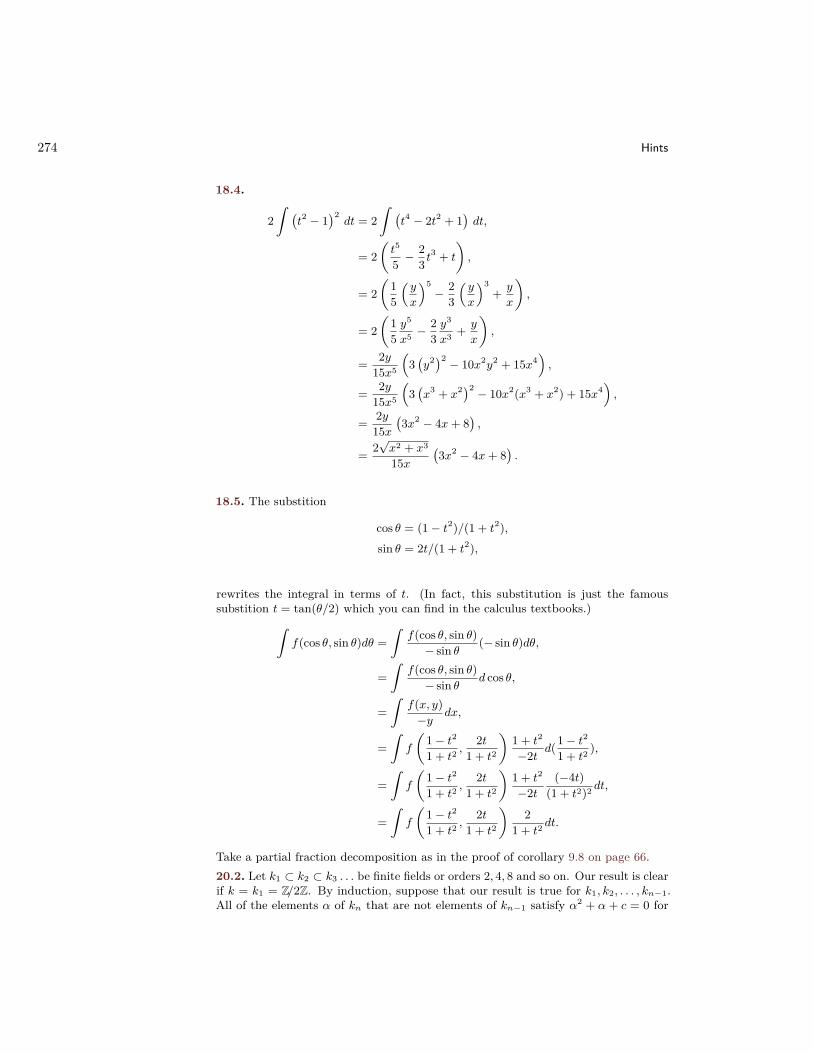
274 Hints

18.4.

2∫ (

t2 − 1)2dt = 2

∫ (t4 − 2t2 + 1

)dt,

= 2(t5

5 −23 t

3 + t

),

= 2(

15

(y

x

)5− 2

3

(y

x

)3+ y

x

),

= 2(

15y5

x5 −23y3

x3 + y

x

),

= 2y15x5

(3(y2)2 − 10x2y2 + 15x4

),

= 2y15x5

(3(x3 + x2)2 − 10x2(x3 + x2) + 15x4

),

= 2y15x

(3x2 − 4x+ 8

),

= 2√x2 + x3

15x(3x2 − 4x+ 8

).

18.5. The substition

cos θ = (1− t2)/(1 + t2),sin θ = 2t/(1 + t2),

rewrites the integral in terms of t. (In fact, this substitution is just the famoussubstition t = tan(θ/2) which you can find in the calculus textbooks.)∫

f(cos θ, sin θ)dθ =∫

f(cos θ, sin θ)− sin θ (− sin θ)dθ,

=∫

f(cos θ, sin θ)− sin θ d cos θ,

=∫

f(x, y)−y dx,

=∫f

(1− t2

1 + t2,

2t1 + t2

)1 + t2

−2t d(1− t2

1 + t2),

=∫f

(1− t2

1 + t2,

2t1 + t2

)1 + t2

−2t(−4t)

(1 + t2)2 dt,

=∫f

(1− t2

1 + t2,

2t1 + t2

)2

1 + t2dt.

Take a partial fraction decomposition as in the proof of corollary 9.8 on page 66.20.2. Let k1 ⊂ k2 ⊂ k3 . . . be finite fields or orders 2, 4, 8 and so on. Our result is clearif k = k1 = Z/2Z. By induction, suppose that our result is true for k1, k2, . . . , kn−1.All of the elements α of kn that are not elements of kn−1 satisfy α2 + α+ c = 0 for

Hints 275

some c in kn−1, as we saw above. By induction, c = b2 for some element b of kn−1.So α2 + α+ b2 = 0, i.e. α2 + b2 = α. Expand out (α+ b)2 to find (α+ b)2 = α.21.2. Take a basis consisting of one element α ∈ K. Then 1 ∈ K is somehow amultiple 1 = aα for some a ∈ k so α = 1/a ∈ k. Any element β of K is β = cα forsome c ∈ k so β ∈ k.21.3. Let n be the degree of p(x). We write each element b(x) in k[x] as a polynomial,but if the polynomial has degree n or more, rewrite it as b(x) = q(x)p(x) + r(x),quotient and remainder. Then every element of K is written as the remainder term,i.e. as a polynomial of degree at most n−1. Hence the elements 1, x, . . . , xn−1 in k[x]map to a spanning set inside K. If not a basis, then there must be some linear relationbetween them, i.e. a lower degree polynomial in x vanishing in K, i.e. vanishingmodulo p(x). But then taking quotient and remainder, we see that this is not possible.Hence K has a basis over k consisting of the images of 1, x, x2, . . . , xn−1 in k[x].23.3. Homogenize to x3 + x2y + xy2 + y3 + x2z = z3, and then set z = 0 to get thehomogeneous equation x3 + x2y + xy2 + y3 = 0. Factor: (x + y)(x2 + y2) = 0. Sox + y = 0, i.e. [x,−x, 0] = [1,−1, 0], or x2 + y2 = 0, which factors over any field kwhich contains an element i so that i2 = −1, as (x− iy)(x+ iy) = 0, i.e. y = ±ix, so[x, ix, 0] = [1, i, 0] and [x,−ix, 0] = [1,−i, 0]. Hence the points of our curve that lieon the line at infinity are [1,−1, 0], [1, i, 0], [1,−i, 0].23.3. Start with the affine plane. Remember (from problem 8.5 on page 54) that youcan use the quadratic formula:

y =−1±

√1− 4(−x3 − x− 1)

2 .

Simplify, using 2−1 = 3 and 4 = −1, to:

y = 3(−1±√−x3 − x)

Note that 02 = 0, 12 = 1, 22 = 4, 32 = 9 = 4, 42 = 16 = 1, so only 0, 1, 4 have squareroots.

• x = 0: −x3 − x = 0, y = −3 = 2, [x, y, z] = [0, 2, 1].

• x = 1: −x3 − x = 3, no square root of 3, no solution.

• x = 2: −x3 − x = −8− 2 = 0, y = −3 = 2, [x, y, z] = [2, 2, 1].

• x = 3: −x3 − x = −27− 3 = 0, y = −3 = 2, [x, y, z] = [3, 2, 1].

• x = 4: −x3 − x = −68 = 2, no square root of 2 no solution.

We still need the points “at infinity”. Homogenize: y2z+ yz2 = x3 +xz2 + z3, and setz = 0: 0 = x3, so x = 0, i.e. [x, y, z] = [0, y, 0], and rescale y to [0, 1, 0]. Final answer:[0, 2, 1], [2, 2, 1], [3, 2, 1], [0, 1, 0].30.2. p(x, y) = (1− xy)2 + x2 over the field k = R.31.14. To have a nonzero element a + ιb being a zero divisor on the left, we wouldneed to have

0 = (a+ ιb)(c+ ιd),= ac− db+ ι (da+ bc) .

276 Hints

Therefore ac = db and da = −bc. Multiplying suitably, dac = ddb and dac = −ccb.So 0 =

(dd+ cc

)b and thus b = 0 or else c = d = 0. But if b = 0 then ac = 0 and

da = 0, so a = 0 or else c = d = 0.To have a nonzero element a+ ιb being a zero divisor on the right, we would need

to have

0 = (c+ ιd)(a+ ιb),= ca− bd+ ι (bc+ da) .

Therefore ca = bd and bc = −da. Multiplying suitably, bca = bbd and bca = −daa.So therefore d = 0 or else a = b = 0. But if d = 0 then ca = 0 and bc = 0, so c = 0.

Bibliography

[1] C. Herbert Clemens, A scrapbook of complex curve theory, second ed., GraduateStudies in Mathematics, vol. 55, American Mathematical Society, Providence,RI, 2003. MR 1946768 (2003m:14001)

[2] David S. Dummit and Richard M. Foote, Abstract algebra, third ed., John Wiley& Sons, Inc., Hoboken, NJ, 2004. MR 2286236 (2007h:00003)

[3] Ronald L. Graham, Donald E. Knuth, and Oren Patashnik, Concrete mathe-matics, second ed., Addison-Wesley Publishing Company, Reading, MA, 1994, Afoundation for computer science. MR 1397498 (97d:68003)

[4] Thomas W. Hungerford, Algebra, Graduate Texts in Mathematics, vol. 73,Springer-Verlag, New York-Berlin, 1980, Reprint of the 1974 original. MR 600654(82a:00006)

[5] Igor R. Shafarevich, Basic notions of algebra, Encyclopaedia of MathematicalSciences, vol. 11, Springer-Verlag, Berlin, 2005, Translated from the 1986 Russianoriginal by Miles Reid, Reprint of the 1997 English translation [MR1634541],Algebra, I. MR 2164721

[6] Michael Spivak, Calculus, Calculus, Cambridge University Press, 2006. 48, 59,64

[7] The Sage Developers, Sagemath, the Sage Mathematics Software System (Version7.5.1), 2018, http://www.sagemath.org.

[8] E. B. Vinberg, A course in algebra, Graduate Studies in Mathematics, vol. 56,American Mathematical Society, Providence, RI, 2003, Translated from the 2001Russian original by Alexander Retakh. MR 1974508 (2004h:00001)

[9] Judy L. Walker, Codes and curves, Student Mathematical Library, vol. 7, Amer-ican Mathematical Society, Providence, RI; Institute for Advanced Study (IAS),Princeton, NJ, 2000, IAS/Park City Mathematical Subseries. MR 1768485(2001f:14046)

[10] André Weil, Number theory for beginners, Springer-Verlag, New York-Heidelberg,1979, With the collaboration of Maxwell Rosenlicht. MR 532370 (80e:10004)

277

List of notation

gcd {m1,m2, . . . ,mn} greatest common divisor, 6lcm {m1,m2, . . . ,mn} least common multiple, 7b congruence class of b, 27b ≡ c (mod m) b is congruent to c modulo m, 27φ(m) Euler’s totient function, 36||z|| modulus of a complex number, 49resb,c resultant of polynomials b(x), c(x), 78p′(x) derivative of polynomial, 84|G| order of group, 96Dn the dihedral group, 97G ∗H amalgation, 110G ∗K H amalgation over a subgroup, 111ej elementary symmetric functions, 114xa multivariable exponent, 117pj sum of powers polynomials, 119R(x) the field of rational functions with coefficients in a ring R, 126k algebraic closure, 134ker f kernel of a ring morphism, 137R ∼= S isomorphic rings, 138(A) ideal generated by a set A in a ring R, 139R/I quotient of a ring by an ideal, 164P2(k) projective plane over a field k, 179Pn(k) projective space over a field k, 180degBC total multiplicity of intersection of curves B and C, 188BCp multiplicity of intersection of curves B and C at point p, 188P ∗ dual projective plane, 240H quaternions, 243P2(O) the octave projective plane, 256

279

Index

∗-ring, 253real, 253

abelian, 94absolute value, 2addition laws, 1, 126, 243, 252affine space, 235affine variety, 237algebra, 141algebraic

closure, 134curve, 148, 149

algorithmEuclidean, 7extended Euclidean, 17

alphabet, 105alternative ring, 253Armstrong, Mark, 89associative law

addition, 1, 126, 252multiplication, 1, 126

associator, 253automorphism, 143

group, 143projective plane, 246ring, 138

Bézoutcoefficients, 17theorem, 189, 191

basis, 131, 244bijection, 89birational, 151biregular, 149Blake, William, 175Boole, George, 9bounded from below, 5Brahma’s correct system, 33Brahma-Sphuta-Siddhanta, 33Brahmagupta, 33

broken Desargues configuration, 249Brothers Karamazov, 176

Carroll, Lewis, 4Cayley graph, 100Cayley, Arthur, 175characteristic, 129characteristic polynomial, 121Chasles theorem, 205Chinese remainder theorem, 138closed set, 237closure, 237coefficient

of polynomial, 51common divisor, 6commutative law

addition, 1, 126, 252multiplication, 1, 127, 252

commuting, 94complex conjugation, 49component, 149

multiple, 186concatentation, 105cone, 181configuration, 245

broken Desargues, 249dual, 247standard Desargues, 249trivalent, 251

conic, 148conjugation, 253coordinates

homogeneous, 178coprime, 6cubic

curve, 148polynomial, 54

curvealgebraic, 148cubic, 148

281

282 Index

degree, 148elliptic, 206irreducible, 149projective plane, 182quartic, 148quintic, 148rational, 152reducible, 149regular, 212smooth, 212

cycle, 92disjoint, 92

cyclic, 98

Dawson, Les, 45De Morgan, Augustus, 51degree

of algebraic curve, 148of field extension, 131, 172of polynomial, 51

denominator, 46derivative, 84Desargues

configurationbroken, 249standard, 249

projective plane, 248Descartes

theorem, 59descriptive geometry, 175determinacy of sign, 2determinant, 91dihedral group, 97Dijkstra, Edsger, 21dimension, 245discriminant, 84distributive law, 1, 126, 252division, 4

by zero, 4divisor, 4Dostoyevsky, Fyodor, 176Douglass, Frederick, 2dragon, 257dual

configuration, 247curve, 234projective plane, 199, 233, 240

elliptic curve, 206equality cancellation law

addition, 3multiplication, 3

Euclid, 5, 17, 24Euclidean algorithm, 7

extended, 17, 18Euler

lemma, 219Euler’s totient function, 36, 42Euler, Leonhard, 25even integer, 24existence of negatives, 1, 126, 252expected number of distinct roots, 62extended Euclidean algorithm, 17, 18extension

Galois, 145simple, 145

Fano plane, 179, 246Fermat’s Last Theorem, 148Fibonacci sequence, 13, 15field, 53, 128

of fractions, 140splitting, 134

fixed point, 105flex, 219form

quadratic, 227free

group, 105product, 110

Frobenius morphism, 168Frost, Robert, 137function

rational, 126, 151recursive, 13regular, 149

Galois extension, 145Galois group, 144Gauss’s lemma, 69Gauss, Carl Friedrich, 27general position, 199generate

projective plane, 251generators, 100generic

triangle, 187very, 187

Graves, Robert, 211greatest common divisor, 6

Index 283

group, 94automorphism, 143Galois, 144isomorphism, 96transformation, 90

Haddon, Mark, 23hair

red, 9Hardy, G. H., 247heaven, vihell, viHessian

curve, 219Hilbert basis theorem, 235homogeneous

coordinates, 178polynomial, 122, 181

homomorphism, 137horse, 12hyperplane

linear, 74

ideal, 139maximal, 165prime, 164

identity lawaddition, 1, 126, 252multiplication, 1, 127, 252

identity transformation, 89image, 108, 245incidence geometry, 245independent conditions, 201induction, 10inequality cancellation law

addition, 4multiplication, 4

inertia, 227inflection point, 219injective, 89

morphism, 138intermediate value theorem, 59interpolation, 57intersection number, 188invariant

of square matrix, 121inverse, 89invertible

transformation, 89irreducible

curve, 149polynomial, 53, 70, 173

isomorphicrings, 138

isomorphismof groups, 96projective plane, 246ring, 138

Karenina, Anna, 195kernel, 108, 245

ring morphism, 137Kirillov, A. A., 54kite, 246Klein, Felix, 147Kronecker, Leopold, 1

Lagrange, Joseph-Louis, 104Lang, Serge, 205law of well ordering, 2, 5, 10least common multiple, 7left coset, 101left translate, 101lemma

Euler, 219line, 148linear

function, 74hyperplane, 74projective automorphism, 247system, 199

linear combination, 244linear map, 245linear relation, 244linear transformation, 91linearly independent, 244list, 14lower bound, 5Lüroth’s theorem, 173

Malraux, André, 41Marx, Chico, 184mathematical induction, 10maximal ideal, 165Mencken, H. L., 64modulus, 49monic polynomial, 53, 113morphism

Frobenius, 168injective, 138

284 Index

of groups, 106one-to-one, 138onto, 138rational, 151regular, 149ring, 137surjective, 138

multiplication laws, 1, 126, 244, 252multiplication table, 96multiplicative inverse, 31

negative, 2neighborhood, 237Newton, Isaac, 120norm, 49nullstellensatz, 236number

rational, 45number line, 48numerator, 46

octave projective plane, 256octaves, 253octonions, 253odd integer, 24one-to-one, 89

morphism, 138onto, 89

morphism, 138open set, 237optics, viorbit, 104order, 96

group element, 98of point on curve, 211

Painlevé, Paul, 48papyrus

Rhind, 45partial fraction, 66, 152

decomposition, 66pencil, 195, 199perfect square, 47permutation, 89perspective, 247, 248Philips, Emo, 13Picasso, Pablo, 8plane, 241

Fano, 179plane curve

projective, 182Plath, Sylvia, 41Poincaré, Henri, 89point

regular, 211singular, 212smooth, 211

polygon, 197, 246polynomial, 51, 126

cubic, 54homogeneous, 122, 181irreducible, 53, 70, 173monic, 53, 113quadratic, 54reducible, 53, 70, 173

positive, 2rational number, 47

presentation, 105prime, 23prime ideal, 164product, 96projective

automorphism, 178, 180line, 177plane, 177, 179, 239

automorphism, 246Desargues, 248dual, 199, 240generation, 251isomorphism, 246

plane curve, 182space, 180, 241subspace, 242

projective planequaternionic, 243

quadraticform, 227polynomial, 54

quadrilateral, 197quartic

curve, 148quaternionic projective plane, 243quaternions, 243quintic

curve, 148quotient, 5quotient ring, 164

rational

Index 285

curve, 152function, 126, 151morphism, 151number, 45

real∗-ring, 253

recursive function, 13red hair, 9reduce, 105reducible

curve, 149polynomial, 53, 70, 173

regularcurve, 212function, 149point, 211

regular point, 151remainder, 5, 42resultant, 78, 135, 157Rhind papyrus, 45right coset, 101right translate, 101ring, 125, 252

alternative, 253roots

expected number, 62Russell, Bertrand, 131, 227, 239

scalar multiplication, 141Shakespeare, William, 239sign laws, 2signature, 227simple extension, 145singular point, 212skew field, 243smooth

curve, 212point, 211

span, 244split polynomial, 133splitting field, 133, 134square-free, 228St. Vincent Millay, Edna, 17standard Desargues configuration, 249Study

theorem, 186Sturm

sequence, 61subgroup, 100subspace, 244

projective, 242subtraction, 3succession, 2surjective, 89

morphism, 138Swift, Jonathan, 9Sylvester’s law of inertia, 227Sylvester, James, 227symmetric

function, 116symmetric group, 91

tangent line, 209temperature, viternary ring, 255tetrahedron, 91theorem

Bézout, 189, 191Chasles, 205Descartes, 59Hilbert basis, 235intermediate value, 59Lüroth, 173nullstellensatz, 236Study, 186

Thom, René, 257Tolstoy, Leo, 195, 239totient function, 36trace, 121transformation, 89

group, 90identity, 89invertible, 89linear, 91

triangle, 197generic, 187very generic, 187

trivalent configuration, 251Twelfth Night, 239

unit, 31ring, 128

varietyaffine, 237

very generictriangle, 187

Vieté, Francois, 114

War and Peace, 239

286 Index

weight, 117, 123well ordering, 2Weyl, Hermann, 113Williams, Tennessee, 69Wittgenstein, Ludwig, vword, 105, 111

zero divisor, 129Zhou, Zhuang, 257Zhuangzi, 257