arX

iv:c

ond-

mat

/040

9439

v1 [

cond

-mat

.sof

t] 1

7 Se

p 20

04

CONFORMAL MAPPING METHODSFOR INTERFACIAL DYNAMICS1

Microstructural evolution is typically beyond the reach of mathematical analysis, but in two

dimensions certain problems become tractable by complex analysis. Via the analogy be-

tween the geometry of the plane and the algebra of complex numbers, moving free boundary

problems may be elegantly formulated in terms of conformal maps. For over half a century,

conformal mapping has been applied to continuous interfacial dynamics, primarily in models

of viscous fingering and solidification. Current developments in materials science include

models of void electro-migration in metals, brittle fracture, and viscous sintering. Recently,

conformal-map dynamics has also been formulated for stochastic problems, such as diffusion-

limited aggregation and dielectric breakdown, which has reinvigorated the subject of fractal

pattern formation.

Although restricted to relatively simple models, conformal-map dynamics offers unique ad-

vantages over other numerical methods discussed in this chapter (such as the Level-Set

Method) and in Chapter 9 (such as the Phase Field Method). By absorbing all geometrical

complexity into a time-dependent conformal map, it is possible to transform a moving free

boundary problem to a simple, static domain, such as a circle or square, which obviates the

need for front tracking. Conformal mapping also allows the exact representation of very

complicated domains, which are not easily discretized, even by the most sophisticated adap-

tive meshes. Above all, however, conformal mapping offers analytical insights for otherwise

intractable problems.

After reviewing some elementary concepts from complex analysis in §1, we consider the clas-

sical application of conformal mapping methods to continous-time interfacial free boundary

problems in §2. This includes cases where the governing field equation is harmonic, bihar-

monic, or in a more general conformally invariant class. In §3, we discuss the recent use of

random, iterated conformal maps to describe analogous discrete-time phenonena of fractal

growth. Although most of our examples involve planar domains, we note in §4 that interfa-

cial dynamics can also be formulated on curved surfaces in terms of more general conformal

maps, such as stereographic projections. We conclude in §5 with some open questions and

an outlook for future research.

1A perspective article to appear in the Handbook of Materials Modeling, ed. by S. Yip et al., Vol. I, Ch.4, Art. 4.10 (Springer Science and Business Media, 2005).

1

1 Analytic functions and conformal maps

We begin by reviewing some basic concepts from complex analysis found in textbooks such

as Churchill and Brown (1990). For a fresh geometrical perspective, see Needham (1997).

A general function of a complex variable depends on the real and imaginary parts, x and y,

or, equivalently, on the linear combinations, z = x+iy and z = x−iy. In contrast, an analytic

function, which is differentiable in some domain, can be written simply as, w = u+iv = f(z).

The condition, ∂f/∂z = 0, is equivalent to the Cauchy-Riemann equations,

∂u

∂x=∂v

∂yand

∂u

∂y= −∂v

∂x, (1)

which follow from the existence of a unique derivative,

f ′ =∂f

∂x=∂u

∂x+ i

∂v

∂x=

∂f

∂(iy)=∂v

∂y− i

∂u

∂y, (2)

whether taken in the real or imaginary direction.

Geometrically, analytic functions correspond to a special mappings of the complex plane. In

the vicinity of any point where the derivative is nonzero, f ′(z) 6= 0, the mapping is locally

linear, dw = f ′(z) dz. Therefore, an infinitessimal vector, dz, centered at z is transformed

into another infinitessimal vector, dw, centered at w = f(z) by a simple complex multi-

plication. Recalling Euler’s formula, (r1eiθ1)(r2e

iθ2) = (r1r2)ei(θ1+θ2), this means that the

mapping causes a local stretch by |f ′(z)| and local rotation by arg f ′(z), regardless of the

orientation of dz. As a result, an analytic function with a nonzero derivative describes a

conformal mapping of the plane, which preserves the angle between any pair of intersecting

curves. Intuitively, a conformal mapping smoothly warps one domain into another with no

local distortion.

Conformal mapping provides a very convenient representation of free boundary problems.

The Riemann Mapping Theorem guarantees the existence of a unique conformal mapping

between any two simply connected domains, but the challenge is to derive its dynamics

for a given problem. The only constraint is that the conformal mapping be univalent, or

one-to-one, so that physical fields remain single-valued in the evolving domain.

2

2 Continuous interfacial dynamics

2.1 Harmonic fields

Most applications of conformal mapping involve harmonic funtions, which are solutions to

Laplace’s equation,

∇2φ = 0. (3)

From Eq. (1), it is easy to show that the real and imaginary parts of an analytic function

are harmonic, but the converse is also true: Every harmonic is the real part of an analytic

function, φ = Re Φ, the complex potential.

This connection easily produces new solutions to Laplace’s equation in different geometries.

Suppose that we know the solution, φ(w) = ReΦ(w), in a simply connected domain in

the w-plane, Ωw, which can be reached by conformal mapping, w = f(z, t), from another,

possibly time-depedent domain in the z-plane, Ωz(t). A solution in Ωz(t) is then given by

φ(z, t) = ReΦ(w) = ReΦ(f(z, t)) (4)

because Φ(f(z)) is also analytic, with a harmonic real part. The only caveat is that the

boundary conditions be invariant under the mapping, which holds for Dirichlet (φ=constant)

or Neumann (n · φ = 0) conditions. Most other boundary conditions invalidate Eq. (4) and

thus complicate the analysis.

The complex potential is also convenient for calculating the gradient of a harmonic function.

Using Eqs. (1) and (2), we have

∇zφ =∂φ

∂x+ i

∂φ

∂y= Φ′, (5)

where ∇z is the complex gradient operator, representing the vector gradient, ∇, in the

z-plane.

Viscous fingering and solidification: The classical application of conformal-map dynam-

ics is to Laplacian growth, where a free boundary, Bz(t), moves with a (normal) velocity,

v =dz

dt∝ ∇φ, (6)

proportional to the gradient of a harmonic function, φ, which vanishes on the boundary

(Howison (1992)). Conformal mapping for Laplacian growth was introduced independently

by Polubarinova-Kochina and Galin in 1945 in the context of groundwater flow, where φ

3

(a) (b)

Figure 1: Exact solutions for Laplacian growth, a simple model of viscous fingering: (a)a Saffman-Taylor finger translating down an infinite channel, showing iso-pressure curves(dashed) and streamlines (solid) in the viscous fluid, and (b) the evolution of a perturbedcircular bubble leading to cusp singularities in finite time. [Courtesy of Jaehyuk Choi.]

is the pressure field and u = (k/η)∇φ is the velocity of the fluid of viscosity, η, in a

porous medium of permeability, k, according to Darcy’s law. Laplace’s equation follows

from incompressibility, ∇ · u = 0. The free boundary represents an interface with a less

viscous, immiscible fluid at constant pressure, which is being forced into the more viscous

fluid.

In physics, Laplacian growth is viewed as a fundamental model for pattern formation. It also

describes viscous fingering in Hele-Shaw cells, where a bubble of fluid, such as air, displaces

a more viscous fluid, such as oil, in the narrow gap between parallel flat plates. In that case,

the depth averaged velocity satisfies Darcy’s law in two dimensions. Laplacian growth also

describes dendritic solidification in the limit of low undercooling, where φ is the temperature

in the melt (Cummings et al. (1999)).

To illustrate the derivation of conformal-map dynamics, let us consider viscous fingering in a

channel with inpenetrable walls, as shown in Fig. 1(a). The viscous fluid domain, Ωz(t), lies

in a periodic horizontal strip, to the right of the free boundary, Bz(t), where uniform flow of

velocity, U , is assumed far ahead of the interface. It is convenient to solve for the conformal

map, z = g(w, t), to this domain from a half strip, Rew > 0, where the pressure is simply

linear, φ = ReUw/µ. We also switch to dimensionless variables, where length is scaled to a

4

characteristic size of the initial condition, L, pressure to UL/µ, and time to L/U .

Since ∇wφ = 1 in the half strip, the pressure gradient at a point, z = g(w, t), on the physical

interface is easily obtained from Eq. (30):

∇zφ =∂f

∂z=

(

∂g

∂w

)−1

(7)

where w = f(z, t) is the inverse mapping (which exists as long as the mapping remains

univalent). Now consider a Lagrangian marker, z(t), on the interface, whose pre-image,

w(t), lies on the imaginary axis in the w-plane. Using the chain rule and Eq. (7), the

kinematic condition, Eq. (6), becomes,

dz

dt=∂g

∂t+∂g

∂w

dw

dt=

(

∂g

∂w

)−1

. (8)

Multiplying by ∂g/∂w 6= 0,this becomes

∂g

∂w

∂g

∂t+

∣

∣

∣

∣

∂g

∂w

∣

∣

∣

∣

2dw

dt= 1. (9)

Since the pre-image moves along the imaginary axis, Re (dw/dt) = 0, we arrive at the

Polubarinova-Galin equation for the conformal map:

Re

(

∂g

∂w

∂g

∂t

)

= 1, for Rew = 0. (10)

From the solution to Eq. (10), the pressure is given by φ = Re f(z, t). Note that the

interfacial dynamics is nonlinear, even though the quasi-steady equations for φ are linear.

The best-known solutions are the Saffman-Taylor fingers,

g(w, t) =t

λ+ w + 2(1 − λ) log(1 + e−w) (11)

which translate at a constant velocity, λ−1, without changing their shape (Saffman and Taylor

(1958)). Note that (11) is a solution to the fingering problem for all choices of the parameter

λ. This parameter specifies the finger width and can be chosen arbitrarily in the solution

(11). In experiments however, it is found that the viscous fingers that form are well fit by

a Saffman-Taylor finger filling precisely half of the channel, that is with λ = 1/2, as shown

in Fig. 1(a). Why this happens is a basic problem in pattern selection, which has been the

focus of much debate in the literature over the last 25 years.

5

Figure 2: Numerical simulation of viscous fingering, starting from a three-fold perturbationof a circular bubble. The only difference with the Laplacian-growth dynamics in Fig. 1(b) isthe inclusion of surface tension, which prevents the formation of cusp singularities. [Courtesyof Michael Siegel.]

To understand this problem, note that the viscous finger solutions (11) do not include any of

the effects of surface tension on the interface between the two fluids. The intriguing pattern

selection of the λ = 1/2 finger has been attributed to a singular perturbation effect of small

surface tension. Surface tension, γ, is a significant complication because it is described by a

non-conformally-invariant boundary condition,

φ = γκ, for z ∈ Bz(t) (12)

where κ is the local interfacial curvature, entering via the Young-Laplace pressure. Small

surface tension can be treated analytically as a singular perturbation to gain insights into

pattern selection (Kruskal and Segur (1991); Tanveer (1993a)). Since surface tension effects

are only significant at points of high curvature κ in the interface, and given that the finger in

6

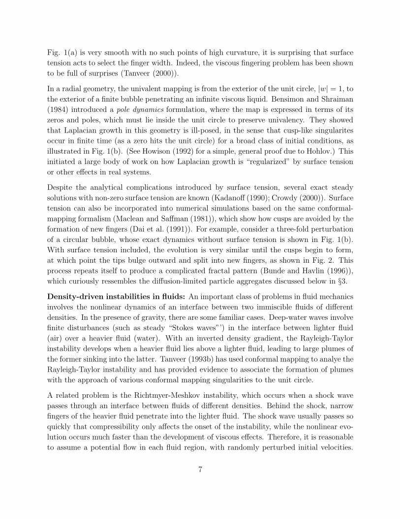
Fig. 1(a) is very smooth with no such points of high curvature, it is surprising that surface

tension acts to select the finger width. Indeed, the viscous fingering problem has been shown

to be full of surprises (Tanveer (2000)).

In a radial geometry, the univalent mapping is from the exterior of the unit circle, |w| = 1, to

the exterior of a finite bubble penetrating an infinite viscous liquid. Bensimon and Shraiman

(1984) introduced a pole dynamics formulation, where the map is expressed in terms of its

zeros and poles, which must lie inside the unit circle to preserve univalency. They showed

that Laplacian growth in this geometry is ill-posed, in the sense that cusp-like singularites

occur in finite time (as a zero hits the unit circle) for a broad class of initial conditions, as

illustrated in Fig. 1(b). (See Howison (1992) for a simple, general proof due to Hohlov.) This

initiated a large body of work on how Laplacian growth is “regularized” by surface tension

or other effects in real systems.

Despite the analytical complications introduced by surface tension, several exact steady

solutions with non-zero surface tension are known (Kadanoff (1990); Crowdy (2000)). Surface

tension can also be incorporated into numerical simulations based on the same conformal-

mapping formalism (Maclean and Saffman (1981)), which show how cusps are avoided by the

formation of new fingers (Dai et al. (1991)). For example, consider a three-fold perturbation

of a circular bubble, whose exact dynamics without surface tension is shown in Fig. 1(b).

With surface tension included, the evolution is very similar until the cusps begin to form,

at which point the tips bulge outward and split into new fingers, as shown in Fig. 2. This

process repeats itself to produce a complicated fractal pattern (Bunde and Havlin (1996)),

which curiously ressembles the diffusion-limited particle aggregates discussed below in §3.

Density-driven instabilities in fluids: An important class of problems in fluid mechanics

involves the nonlinear dynamics of an interface between two immiscible fluids of different

densities. In the presence of gravity, there are some familiar cases. Deep-water waves involve

finite disturbances (such as steady “Stokes waves”’) in the interface between lighter fluid

(air) over a heavier fluid (water). With an inverted density gradient, the Rayleigh-Taylor

instability develops when a heavier fluid lies above a lighter fluid, leading to large plumes of

the former sinking into the latter. Tanveer (1993b) has used conformal mapping to analye the

Rayleigh-Taylor instability and has provided evidence to associate the formation of plumes

with the approach of various conformal mapping singularities to the unit circle.

A related problem is the Richtmyer-Meshkov instability, which occurs when a shock wave

passes through an interface between fluids of different densities. Behind the shock, narrow

fingers of the heavier fluid penetrate into the lighter fluid. The shock wave usually passes so

quickly that compressibility only affects the onset of the instability, while the nonlinear evo-

lution occurs much faster than the development of viscous effects. Therefore, it is reasonable

to assume a potential flow in each fluid region, with randomly perturbed initial velocities.

7

Figure 3: Conformal-map dynamics for the strongly nonlinear regime of the Richtmyer-Meshkov instability (Yoshikawa and Balk (1999)). [Courtesy of Toshio Yoshikawa andAlexander Balk.]

Although real plumes roll up in three dimensions and bubbles can form, conformal mapping

in two dimensions still provides some insights, with direct relevance for shock tubes of high

aspect ratio.

A simple conformal-mapping analysis is possible for the case of a large density contrast, where

the lighter fluid is assumed to be at uniform pressure. The Richtmyer-Meshkov instability

(zero-gravity limit) is then similar to the Saffman-Taylor instability, except that the total

volume of each fluid is fixed. A periodic interface in the y direction, analogous to the channel

geometry in Fig. 1, can be described by the univalent mapping, z = g(w, t), from the interior

of the unit circle in the mathematical w plane to the interior of the heavy-fluid finger in the

physical z plane.

Zakharov (1968) introduced a Hamiltonian formulation of the interfacial dynamics in terms

of this conformal map, taking into account kinetic and potential energy, but not surface

tension. One way to derive equations of motion is to expand the map in a Taylor series,

g(w, t) = logw +

∞∑

n=0

an(t)wn, |w| < 1. (13)

8

(The logw term first maps the disk to a periodic half strip.) On the unit circle, w = eiθ, the

pre-image of the interface, this is simply a complex Fourier series. The Taylor coefficients,

an(t), act generalized coordinates describing n-fold shape perturbations within each period,

and their time derivatives, an(t), act as velocities or momenta. Unfortunately, truncating

the Taylor series results in a poor description of strongly nonlinear dynamics because the

conformal map begins to vary wildly near the unit circle.

An alternate approach used by Yoshikawa and Balk (1999) is to expand in terms ressembling

Saffman-Taylor fingers,

g(w, t) = logw + b(t) −N∑

n=1

bn(t) log(1 − λn(t)w) (14)

which can be viewed as a resummation of the Taylor series in Eq. (13). As shown in Fig. 3,

exact solutions exist with only a finite number terms in the finger expansion, as long as

the new generalized coordinates, λn(t), stay inside the unit disk, |λn| < 1. This example

illustrates the importance of the choice of shape functions in the expansion of the conformal

map, e.g. wn versus log(1 − λnw).

Void electro-migration in metals: Micron-scale interconnects in modern integrated cir-

cuits, typically made of aluminum, sustain enormous currents and high temperatures. The

intense electron wind drives solid-state mass diffusion, especially along dislocations and grain

boundaries, where voids also nucleate and grow. In the narrowest and most fragile inter-

connects, grain boundaries are often well separated enough that isolated voids migrate in a

fairly homogeneous environment due to surface diffusion, driven by the electron wind. Voids

tend to deform into slits, which propagate across the interconnect, causing it to sever. A

theory of void electro-migration is thus important for predicting reliability.

In the simplest two-dimensional model (Wang et al. (1996)), a cylindrical void is modeled as

a deformable, insulating inclusion in a conducting matrix. Outside the void, the electrostatic

potential, φ, satisfies Laplace’s equation, which invites the use of conformal mapping. The

electric field, E = −∇φ, is taken to be uniform far away and wraps around the void surface,

due to a Neuman boundary condition, n ·E = 0.

The difference with Laplacian growth lies in the kinematic condition, which is considerably

more complicated. In place of Eq. (6), the normal velocity of the void surface is given by

the surface divergence of the surface current, j, which takes the dimensionless form,

n · v =∂j

∂s= χ

∂2φ

∂s2+∂2κ

∂s2(15)

where s is the local arc-length coordinate and χ is a dimensionless parameter comparing

9

(a) (b)

Figure 4: Numerical conformal-mapping simulations of the electromigration of voids inaluminum interconnects (Wang et al. (1996)). (a) A small shape perturbation of a cylindricalvoid decaying (above) or deforming into a curved slit (below), depending on a dimensionlessgroup, χ, comparing the electron wind to surface-tension gradients. (b) A void evolving withanisotropic surface diffusivity (χ = 100, gd = 100, m = 3). [Courtesy of Zhigang Suo.]

surface currents due to the electron wind force (first term) and due to gradients in surface

tension (second term). This moving free boundary problem somewhat resembles the viscous

fingering problem with surface tension, and it admits analogous finger solutions, albeit of

width 2/3, not 1/2 (Ben Amar (1999)).

To describe the evolution of a singly connected void, we consider the conformal map, z =

g(w, t), from the exterior of the unit circle to the exterior of the void. As long as the map

remains univalent, it has a Laurent series of the form,

g(w, t) = A1(t)w + A0(t) +

∞∑

n=1

A−n(t)w−n, for|w| > 1, (16)

where the Laurent coefficients, An(t), are now the generalized coordinates. As in the case of

viscous fingering (Howison (1992)), a hierarchy of nonlinear ordinary differential equations

(ODEs) for these coordinates can be derived. For void electromigration, Wang et al. (1996)

start from a variational principle accounting for surface tension and surface diffusion, using

a Galerkin procedure. They truncate the expansion after 17 coefficients, so their numerical

method breaks down if the void deforms significantly, e.g. into curved slit. Nevertheless, as

shown in Fig,. 4(a), the numerical method is able to capture essential features of the early

stages of strongly nonlinear dynamics.

10

In the same regime, it is also possible to incorporate anisotropic surface tension or surface

mobility. The latter involves multiplying the surface current by a factor (1 + gd cosmα),

where α is the surface orientation in the physical z plane, given at z = g(eiθ, t), by

α = θ + arg∂g

∂w(eiθ, t). (17)

Some results are shown in Fig. 4(b), where the void develops dynamical facets.

Quadrature domains: We end this section by commenting on some of the mathematics

underlying the existence of exact solutions to continuous-time Laplacian-growth problems.

Significantly, much of this mathematics carries over to problems in which the governing field

equation is not necessarily harmonic, as will be seen in the following section.

The steadily-translating finger solution (11) of Saffman and Taylor turns out to be but one of

an increasingly large number of known exact solutions to the standard Hele-Shaw problem.

Saffman (1959) himself identified a class of unsteady finger-like solutions. This solution was

later generalized by Howison (1986) to solutions involving multiple fingers exhibiting such

phenomena as tip-splitting where a single finger splits into two (or more) fingers. It is even

possible to find exact solutions to the more realistic case where there is a second interface

further down the channel (Crowdy and Tanveer (2004)) which must always be the case in

any experiment.

Besides finger-like solutions which are characterized by time-evolving conformal mappings

having logarithmic branch-point singularities, other exact solutions, where the conformal

mappings are rational functions with time-evolving poles and zeros, were first identified by

Polubarinova-Kochina and Galin in 1945. Richardson (1981) later rediscovered the latter

solutions while simultaneously presenting important new theoretical connections between

the Hele-Shaw problem and a class of planar domains known as quadrature domains. The

simplest example of a quadrature domain is a circular disc D of radius r centred at the origin

which satisfies the identity∫ ∫

D

h(z)dxdy = πr2h(0) (18)

where h(z) is any function analytic in the disc (and integrable over it). Equation (18), which

is known as a quadrature identity since it holds for any analytic function h(z), is simply a

statement of the well-known mean-value theorem of complex analysis (Carrier et al. (1966)).

A more general domain D, satisfying a generalized quadrature identity of the form

∫ ∫

D

h(z)dxdy =

N∑

k=1

nk−1∑

j=0

cjkh(j)(zk) (19)

11

is known as a quadrature domain. Here, zk ∈ C is a set of points inside D and h(j)(z)

denotes the j-th derivative of h(z). If one makes the choice h(z) = zn in (19) the resulting

integral quantities have become known as the Richardson moments of the domain. Richard-

son showed that the dynamics of the Hele-Shaw problem is such as to preserve quadrature

domains. That is, if the initial fluid domain in a Hele-Shaw cell is a quadrature domain at

time t = 0, it remains a quadrature domain at later times (so long as the solution does not

break down). This result is highly significant and provides a link with many other areas of

mathematics including potential theory, the notion of balayage, algebraic curves, Schwarz

functions and Cauchy transforms. Richardson (1992) discusses many of these connections

while Varchenko and Etingof (1992) provide a more general overview of the various mathe-

matical implications of Richardson’s result. Shapiro (1992) gives more general background

on quadrature domain theory.

It is a well-known result in the theory of quadrature domains (Shapiro (1992)) that simply-

connected quadrature domains can be parametrized by rational function conformal mappings

from a unit circle. Given Richardson’s result on the preservation of quadrature domains,

this explains why Polubarinova-Kochina and Galin were able to find time-evolving rational

function conformal mapping solutions to the Hele-Shaw problem. It also underlies the pole

dynamics results of Bensimon and Shraiman (1984). But Richardson’s result is not restricted

to simply-connected domains; multiply-connected quadrature domains are also preserved by

the dynamics. Physically this corresponds to time-evolving fluid domains containing mul-

tiple bubbles of air. Indeed, motivated by such matters, recent research has focused on

the analytical construction of multiply-connected quadrature domains using conformal map-

ping ideas (Richardson (2001), Crowdy and Marshall (2004)). In the higher-connected case,

the conformal mappings are no longer simply rational functions but are given by conformal

maps that are automorphic functions (or, meromorphic functions on compact Riemann sur-

faces). The important point here is that understanding the physical problem from the more

general perspective of quadrature domain theory has led the way to the unveiling of more

sophisticated classes of exact conformal mapping solutions.

2.2 Bi-Harmonic fields

Although not as well known as conformal mapping of harmonic functions, there is also a

substantial literature on complex-variable methods to solve the bi-harmonic equation,

∇2∇

2ψ = 0, (20)

which arises in two-dimensional elasticity (Muskhelishvili (1953)) and fluid mechanics (Batchelor

(1967)). Unlike harmonic functions, which can be expressed in terms of a single analytic

12

Figure 5: Evolution of the solution of Hopper (1990) for the coalescence of two equal blobsof fluid under the effects of surface tension.

function (the complex potential), bi-harmonic functions can be expressed in terms of two

analytic functions, f(z) and g(z), in Goursat form (Carrier et al. (1966)):

ψ(z, z) = Im [zf(z) + g(z)] (21)

Note that ψ is no longer just the imaginary part of an analytic function g(z) but also

contains the imaginary part of the non-analytic component zf(z). A difficulty with bi-

harmonic problems is that the typical boundary conditions (see below) are not conformally

invariant, so conformal mapping does not usually generate new solutions by simply a change

of variables, as in Eq. (4). Nevertheless, the Goursat form of the solution, Eq. (21), is a

major simplification, which enables analytical progress.

Viscous sintering: Sintering describes a process by which a granular compact of particles

(e.g. metal or glass) is raised to a sufficiently large temperature that the individual particles

become mobile and release surface energy in such a way as to produce inter-particulate bonds.

At the start of a sinter process, any two particles which are initially touching develop a thin

“neck” which, as time evolves, grows in size to form a more developed bond. In compacts in

which the packing is such that particles have more than one touching neighbour, as the necks

grow in size, the sinter body densifies and any enclosed pores between particles tend to close

up. The macroscopic material properties of the compact at the end of the sinter process

depend heavily on the degree of densification. In industrial application, it is crucial to be

able to obtain accurate and reliable estimates of the time taken for pores to close (or reduce

to a sufficiently small size) within any given initial sinter body in order that industrial sinter

times are optimized without compromising the macroscopic properties of the final densified

sinter body.

The fluid is modelled as a region D(t) of very viscous, incompressible fluid, in which the

velocity field,

u = (u, v) = (ψy,−ψx). (22)

is given by the curl of an out-of-plane vector, whose magnitude is a stream function, ψ(x, y, t),

which satisfies the bi-harmonic equation (Batchelor (1967)). On the boundary ∂D(t), the

13

tangential stress must vanish and the normal stress must be balanced by the uniform surface

tension effect, i.e.,

− pni + 2µeij = Tκni, (23)

where p is the fluid pressure, µ is the viscosity, T is the surface tension parameter, κ is the

boundary curvature, ni denotes components of the outward normal n to ∂D(t) and eij is

the usual fluid rate-of-strain tensor. The boundary is time-evolved in a quasi-steady fashion

with a normal velocity, Vn, determined by the same kinematic condition, Vn = u · n, as in

viscous fingering.

In terms of the Goursat functions in (21) – which are now generally time-evolving – the

stress condition (23) takes the form

f(z, t) + zf ′(z, t) + g′(z, t) = − i

2zs (24)

where again s denotes arclength. Once f(z, t) has been determined from (24), the kinematic

condition

Im[ztzs] = Im[−2f(z, t)zs] −1

2(25)

is used to time-advance the interface.

A significant contribution was made by Hopper (1990) who showed, using complex variable

methods based on the decomposition (21), that the problem for the surface-tension driven

coalescence of two equal circular blobs of viscous fluid can be reduced to the evolution of a

rational function conformal map, from a unit w-circle, of the form

g(w, t) =R(t)w

w2 − a2(t). (26)

The two time-evolving parameters R(t) and a(t) satisfy two coupled nonlinear ODEs. Figure

5 shows a sequence of shapes of the two coalescing blobs computed using Hopper’s solution.

At large times, the configuration equilibrates to a single circular blob.

While Hopper’s coalescence problem provides insight into the growth of the interparticle

neck region, there are no pores in this configuration and it is natural to ask whether more

general exact solutions exist. Crowdy (1999) reappraised the viscous sintering problem and

showed, in direct analogy with Richardson’s result on Hele-Shaw flows, that the dynamics

of the sintering problem is also such as to preserve quadrature domains. As in the Hele-

Shaw problem, this perspective paved the way for the identification of new exact solutions,

generalizing (26), for the evolution of doubly-connected fluid regions. Figure 6 shows the

shrinkage of a pore enclosed by a typical “unit” in a doubly-connected square packing of

touching near-circular blobs of viscous fluid. This calculation employs a conformal mapping

14

Figure 6: The coalescence of fluid blobs and collapse of cylindrical pores in a model ofviscous sintering. This sequence of images shows an analytical solution by Crowdy (2003)using complex-variable methods.

to the doubly-connected fluid region (which is no longer a rational function but a more general

automorphic function) derived by Crowdy (2003) and, in the same spirit as Hopper’s solution

(26), requires only the integration of three coupled nonlinear ODEs. The fluid regions

shown in Figure 6 are all doubly-connected quadrature domains. Richardson (2000) has also

considered similar Stokes flow problems using a different conformal mapping approach.

Pores in elastic solids: Solid elasticity in two dimensions is also governed by a bi-harmonic

function, the Airy stress function (Muskhelishvili (1953)). Therefore, the stress tensor, σij ,

and the displacement field, ui, may be expressed in terms of two analytic functions, f(z)

and g(z):

σ22 + σ11

2= f ′(z) + f ′(z) (27)

σ22 − σ11

2+ iσ12 = zf ′′(z) + g′(z) (28)

Y

1 + ν(u1 + iu2) = κf(z) − zf ′(z) − g(z) (29)

where Y is Young’s modulus, ν is Poisson’s ratio, and κ = (3−ν)/(1+ν) for plane stress and

κ = 3 − 4ν for plane strain. As with bubbles in viscous flow, the use of Goursat functions

allows conformal mapping to be applied to bi-harmonic free boundary problems in elastic

solids, without solving explicitly for bulk stresses and strains.

For example, Wang and Suo (1997) have simulated the dynamics of a singly-connected pore

15

by surface diffusion in an infinite stressed elastic solid. As in the case of void electromigration

described above, they solve nonlinear ODEs for the Laurent coefficients of the conformal map

from the exterior of the unit disk, Eq. (16). Under uniaxial tension, there is a competition

between surface tension, which prefers a circular shape, and the applied stress, which drives

elongation and eventually fracture in the transverse direction. The numerical method, based

on the truncated Laurent expansion, is able to capture the transition from stable elliptical

shapes at small applied stress to the unstable growth of transverse protrusions at large

applied stress, although naturally it breaks down when cusps ressembling crack tips begin

to form.

2.3 Non-harmonic conformally invariant fields

The vast majority of applications of conformal mapping fall into one of the two classes above,

involving harmonic or bi-harmonic functions, where the connections with analytic functions,

Eqs. (4) and (21), are cleverly exploited. It turns out, however, that conformal mapping can

be applied just as easily to a broad class of problems involving non-harmonic fields, recently

discovered by Bazant (2004). Of course, in planar geometry, the conformal map itself is

described by an analytic function, but the fields need not be, as long as they transform in a

simple way under conformal mapping.

The most convenient fields satisfy conformally invariant partial differential equations (PDEs),

whose forms are unaltered by a conformal change of variables. It is straightforward to trans-

form PDEs under a conformal mapping of the plane, w = f(z), by expressing them in terms

of complex gradient operator introduced above,

∇z =∂

∂x+ i

∂

∂y= 2

∂

∂z, (30)

which we have related to the z partial derivative using the Cauchy-Riemann equations,

Eq. (1). In this form, it is clear that ∇zf = 0 if and only if f(z) is analytic, in which case

∇zf = 2f ′. Using the chain rule, also obtain the transformation rule for the gradient,

∇z = f ′ ∇w (31)

To apply this formalism, we write Laplace’s equation in the form,

∇2zφ = Re∇z∇zφ = ∇z∇zφ = 0, (32)

which assumes that mixed partial derivatives can be taken in either order. (Note that

a · b = Re ab.) The conformal invariance of Laplace’s equation, ∇w∇wφ = 0, then follows

16

from a simple calculation,

∇z∇z = (∇zf′)∇w + |f ′|2∇w∇w = |f ′|2 ∇w∇w (33)

where ∇zf′ = 0 because f ′ is also analytic. As a result of conformal invariance, any harmonic

function in the w plane, φ(w), remains harmonic in the z plane, φ(f(z)), after the simple

substitution, w = f(z). We came to the same conclusion above in Eq. (4), using the

connection between harmonic and analytic functions, but the argument here is more general

and also applies to other PDEs.

The bi-harmonic equation is not conformally invariant, but some other equations – and

systems of equations – are. The key observation is that any “product of two gradients”

transforms in the same way under conformal mapping, not only the Laplacian, ∇ ·∇φ, but

also the term, ∇φ1 · ∇φ2 = Re (∇φ1)∇φ2, which involves two real functions, φ1 and φ2:

Re (∇zφ1)∇zφ2 = |f ′|2 Re (∇wφ1)∇wφ2. (34)

(Todd Squires has since noted that the operator, ∇φ1×∇φ2 = Im (∇φ1)∇φ2, also transforms

in the same way.) These observations imply the conformal invariance of a broad class of

systems of nonlinear PDEs:

N∑

i=1

(

ai ∇2φi +

N∑

j=i

aij ∇φi · ∇φj +N∑

j=i+1

bij ∇φi × ∇φj

)

= 0 (35)

where the coefficients ai(φ), aij(φ), and bij(φ) may be nonlinear functions of the unknowns,

φ = (φ1, φ2, . . . , φN), but not of the independent variables or any derivatives of the unknowns.

The general solutions to these equations are not harmonic and thus depend on both z and

z. Nevertheless, conformal mapping works in precisely the same way: A solution, φ(w,w),

can be mapped to another solution, φ(f(z), f(z)), by a simple substitution, w = f(z). This

allows the conformal mapping techniques above (and below) to be extended to new kinds of

moving free boundary problems.

Transport-limited growth phenomena: For physical applications, the conformally in-

variant class, Eq. (35), includes the important set of steady conservation laws for gradient-

driven flux densities,

∂ci∂t

= ∇ · Fi = 0, Fi = ci ui −Di(ci) ∇ci, ui ∝ ∇φ (36)

where ci are scalar fields, such as chemical concentrations or temperature, Di(ci) are

nonlinear diffusivities, ui are irrotational vector fields causing advection, and φ is a poten-

17

Figure 7: The exact self-similar solution, Eq. (40), for continuous advection-diffusion-limitedgrowth in a uniform background potential flow (yellow streamlines) at the dynamical fixedpoint (Pe = ∞). The concentration field (color contour plot) is shown for Pe = 100.[Courtesy of Jaehyuk Choi.]

tial (Bazant (2004)). Physical examples include advection-diffusion, where φ is the harmonic

velocity potential, and electrochemical transport, where φ is the non-harmonic electrostatic

potential, determined implicitly by electro-neutrality.

By modifying the classical methods described above for Laplacian growth, conformal-map

dynamics can thus be formulated for more general, transport-limited growth phenomena

(Bazant et al. (2003)). The natural generalization of the kinematic condition, Eq. (6), is

that the free boundary moves in proportion to one of the gradient-driven fluxes with velocity,

v ∝ F1. For the growth of a finite filament, driven by prescribed fluxes and/or concentrations

at infinity, one obtains a generalization of the Polubarinova-Galin equation for the conformal

map, z = g(w, t), from the exterior of the unit disk to the exterior of growing object,

Re (w g′ gt) = σ(w, t), on |w| = 1 (37)

where σ(w, t) is the non-constant, time-dependent normal flux, n · F1, on the unit circle in

the mathematical plane.

Solidification in a fluid flow: A special case of the conformally invariant equations (35)

has been known for almost a century: steady advection-diffusion of a scalar field, c, in a

18

potential flow, u. The dimensionless PDEs are

Pe u · ∇c = ∇2c, u = ∇φ, ∇

2φ = 0 (38)

where we have introduced the Peclet number, Pe = UL/D, in terms of a characteristic

length, L, velocity, U , and diffusivity, D. In 1905, Boussinesq showed that Equation (38)

takes a simpler form in streamline coordinates, (φ, ψ), where Φ = φ + iψ is the complex

velocity potential:

Pe∂c

∂φ=

(

∂2c

∂φ2+∂2c

∂ψ2

)

(39)

because advection (the left hand side) is directed only along streamlines, while diffusion

(the right hand side) also occurs in the transverse direction, along isopotential lines. From

the general perspective above, we recognize this as the conformal mapping of an invariant

system of PDEs of the form (36) to the complex Φ plane, where the flow is uniform and any

obstacles in the flow are mapped to horizontal slits.

Streamline coordinates form the basis for Maksimov’s method for interfacial growth by

steady advection-diffusion in a background potential flow, which has been applied to freez-

ing in groundwater flow and vapor deposition on textile fibers (Kornev and Mukhamadullina

(1994); Cummings et al. (1999)). The growing interface is a streamline held at a fixed con-

centration (or temperature) relative to the flowing bulk fluid at infinity. This is arguably

the simplest growth model with two competing transport processes, and yet open questions

remain about the nonlinear dynamics, even without surface tension.

The normal flux distribution to a finite absorber in a uniform background flow, σ(w, t) in

Eq. (37) is well known, but rather complicated (Choi et al. (2004b)), so it is replaced by

asymptotic approximations for analytical work, such as σ ∼ 2√

Pe /π sin(θ/2) as Pe → ∞,

which is the fixed point of the dynamics. In this important limit, Choi et al. (2004a) have

found an exact similarity solution,

g(w, t) = A1(t)√

w(w − 1), A1(t) = t2/3 (40)

to Eq. (37) with σ(eiθ, t) =√

A1(t) sin(θ/2) (since Pe (t) ∝ A1(t) for a fixed background

flow). As shown in Figure 7, this corresponds to a constant shape, whose linear size grows

like t2/3, with a 90 cusp at the rear stagnation point, where a branch point of√

w(w − 1)

lies on the unit circle. For any finite, Pe (t), however, the cusp is smoothed, and the map

remains univalent, although other singularities may form. Curiously, when mapped to the

channel geometry with log z, the solution (40) becomes a Saffman-Taylor finger of width,

λ = 3/4.

19

3 Stochastic interfacial dynamics

The continuous dynamics of conformal maps is a mature subject, but much attention is now

focusing on analogous problems with discrete, stochastic dynamics. The essential change

is in the kinematic condition: The expression for the interfacial velocity, e.g. Eq. (6), is

re-interpretted as the probability density (per unit arc length) for advancing the interface

with a discrete “bump”, e.g. to model a depositing particle. Continuous conformal-map

dynamics is then replaced by rules for constructing and composing the bumps. This method

of iterated conformal maps was introduced by Hastings and Levitov (1998) in the context of

Laplacian growth.

Stochastic Laplacian growth has been discussed since the early 1980s, but Hastings and Levitov

(1998) first showed how to implement it with conformal mapping. They proposed the fol-

lowing family of bump functions,

fλ,θ(w) = eiθfλ

(

e−iθw)

, |w| ≥ 1 (41)

fλ(w) = w1−a

[

(1 + λ)(w + 1)

2w

(

w + 1 +

√

w2 + 1 − 2w1 − λ

1 + λ

)

− 1

]a

(42)

as elementary univalent mappings of the exterior of the unit disk used to advance the interface

(0 < a ≤ 1). The function, fλ,θ(w), places a bump of (approximate) area, λ, on the unit

circle, centered at angle, θ. Compared to analytic functions of the unit disk, the Hastings-

Levitov function (42) generates a much more localized perturbation, focused on the region

between two branch points, leaving the rest of the unit circle unaltered (Davidovitch et al.

(1999)). For a = 1, the map produces a strike, which is a line segment of length√λ

emanating normal to the circle. For a = 1/2, the map is an invertible composition of simple

linear, Mobius and Joukowski transformations, which inserts a semi-circular bump on the

unit circle. As shown in Figure 8, this yields a good description of aggregating particles,

although other choices, like a = 2/3, have also been considered (Davidovitch et al. (1999)).

Quantifying the effect of the bump shape remains a basic open question.

Once the bump function is chosen, the conformal map, z = gn(w), from the exterior of the

unit disk to the evolving domain with n bumps is constructed by iteration,

gn(w) = gn−1 (fλn,θn(w)) (43)

starting from the initial interface, given by g0(w). All of the physics is contained in the

sequence of bump parameters, (λn, θn), which can be generated in different ways (in the

w plane) to model a variety of physical processes (in the z plane). As shown in Figure 8(b),

the interface often develops a very complicated, fractal structure, which is given, quite re-

20

(a) (b)

Figure 8: Simulation of the aggregation of (a) 4 and (b) 10,000 particles using the Hastings-Levitov algorithm (a = 1/2). Color contours show the quasi-steady concentration (or prob-ability) field for mobile particles arriving from infinity, and purple curves indicate lines ofdiffusive flux (or probability current). [Courtesy of Jaehyuk Choi and Benny Davidovitch.]

markably, by an exact mapping of the unit circle.

The great advantage of stochastic conformal mapping over atomistic or Monte Carlo simu-

lation of interfacial growth lies in its mathematical insight. For example, given the sequence

(λn, θn) from a simulation of some physical growth process, the Laurent coefficients, Ak(n),

of the conformal map, gn(w), as defined in Eq. (16), can be calculated analytically. For the

bump function (42), Davidovitch et al. (1999) provide a hierarchy of recursion relations,

yielding formulae such as

A1(n) =

n∏

m=1

(1 + λm)a, (44)

and explain how to interpret the Laurent coefficients. For example, A1 is the conformal radius

of the cluster, a convenient measure of its linear extent. It is also the radius of a grounded

disk with the same capacitance (with respect to infinity) as the cluster. The Koebe “1/4

theorem” on univalent functions (Duren (1983)) ensures that the cluster (image of the unit

disk) is always contained in a disk of radius 4A1. The next Laurent coefficient, A0, is the

center of a uniformly charged disk, which would have the same asymptotic electric field as

the cluster (if also charged). Similarly, higher Laurent coefficients encode higher multipole

moments of the cluster.

21

Mapping the unit circle with a truncated Laurent expansion defines the web, which wraps

around the growing tips and exhibits a sort of turbulent dynamics, endlessly forming and

smoothing cusp-like protrusions (Hastings (1997); Hastings and Levitov (1998)). The stochas-

tic dynamics, however, does not suffer from finite-time singularities because the iterated map,

by construction, remains univalent. In some sense, discreteness plays the role of surface ten-

sion, as an another regularization of ill-posed continuum models like Laplacian growth.

Diffusion-Limited Aggregation (DLA): The stochastic analog of Laplacian growth is

the DLA model of Witten and Sander (1981), illustrated in Figure 8, in which particles

perform random walks one-by-one from inifinity until they stick irreversibly to a cluster,

which grows from a seed at the origin. DLA and its variants (see below) provide simple

models for many fractal patterns in nature, such as colloidal aggregates, dendritic electro-

deposits, snowflakes, lightning strikes, mineral deposits, and surface patterns in ion-beam

microscopy (Bunde and Havlin (1996)). In spite of decades of research, however, DLA still

presents theoretical mysteries, which are just beginning to unravel (Halsey (2000)).

The Hastings-Levitov algorithm for DLA prescribes the bump parameters, (λn, θn), as

follows. As in Laplacian growth, the harmonic function for the concentration (or probability

density) of the next random walker approaching an n-particle cluster is simply,

φn(z) = ARe log g−1n (z), (45)

according to Eq. (4), since φ(w) = ARe logw = log |w| is the (trivial) solution to Laplace’s

equation in the mathematical w plane with φ = 0 on the unit disk with a circularly symmetric

flux density, A, prescribed at infinity. Using the transformation rule, Eq. (31), we then find

that the evolving harmonic measure, pn(z)|dz|, for the nth growth event corresponds to a

uniform probability measure, Pn(θ)dθ, for angles, θn, on the unit circle, w = eiθ:

pn(z)|dz| = |∇zφ||dz| =

∣

∣

∣

∣

∣

∇wφ

g′n−1

∣

∣

∣

∣

∣

|g′n−1 dw| = |∇wφ||dw| =dθ

2π= Pn(θ)dθ, (46)

where we set A = 1/2π for normalization, which implicitly sets the time scale (see below).

The conformal invariance of the harmonic measure is well known in mathematics, but the

surprising result of Hastings and Levitov (1998) is that all the complexity of DLA is slaved

to a sequence of independent, uniform random variables.

Where the complexity resides is in the bump area, λn, which depends non-trivially on current

cluster geometry and thus on the entire history of random angles, θm|m ≤ n. For DLA,

the bump area in the mathematical w plane should be chosen such that it has a fixed value,

λ0, in the physical z plane, equal to the aggregating particle area. As long as the new bump

22

is sufficiently small, it is natural to try to correct only for the Jacobian factor

Jn(w) = |g′n(w)|2 =

n∏

m=1

|g′λm,θm(w)|2 (47)

of the previous conformal map at the center of the new bump,

λn =λ0

Jn−1(eiθn), (48)

although it is not clear a priori that such a local approximation is valid. Note at least that

g′n → ∞, and thus λn → 0, as the cluster grows, so this has a chance of working.

Numerical simulations with the Hastings-Levitov algorithm do indeed produce nearly con-

stant bump areas, as in Figure 8. Nevertheless, much larger “particles”, which fill deep fjords

in the cluster, occasionally occur where the map varies too wildly, as shown in Figure 9(a). It

is possible (but somewhat unsatisfying) to reject particles outside an “area acceptance win-

dow” to produce rather realistic DLA clusters, as shown in Figure 9(b). It seems that the

rejected large bumps are so rare that they do not much influence statistical scaling properties

of the clusters (Stepanov and Levitov (2001)), although this issue is by no means rigorously

resolved.

Fractal geometry: Fractal patterns abound in nature, and DLA provides the most com-

mon way to understand them Bunde and Havlin (1996). The fractal scaling of DLA has

been debated for decades, but conformal dynamics is shedding new light on the problem.

Simulations show that the conformal radius (44) exhibits fractal scaling, A1(n) ∝ n1/Df ,

where the fractal dimension, Df = 1.71, agrees with the accepted value from Monte Carlo

(random walk) simulations of DLA, although the prefactor seems to depend on the bump

function (Davidovitch et al. (1999)). A perturbative renormalization-group analysis of the

conformal dynamics by Hastings (1997) gives a similar result, Df = 2−1/2+1/5 = 1.7. The

multifractal spectrum of the harmonic measure has also been studied (Jensen et al. (2002);

Ball and Somfai (2002)).

Perhaps the most basic question is whether DLA clusters are truly fractal – statistically self-

similar and free of any length scale. This long-standing question requires accurate statistics

and very large simulations, to erase the surprisingly long memory of the initial conditions.

Conformal dynamics provides exact formulae for cluster moments, but simulations are limited

to at most 105 particles by poor O(n2) scaling, caused by the history-dependent Jacobian

in Eq. (48). In contrast, efficient random-walk simulations can aggregate many millions of

particles.

Therefore, Somfai et al. (1999) developed a hybrid method relying only upon the existence of

23

(a) (b)

-

(c)

-

(d)

-

(e)

-

(f)

-

Figure 9: Simulations of fractal aggregates by Stepanov and Levitov (2001): (a) Super-imposed time series of the boundary, showing the aggregation of particles, represented byiterated conformal maps; (b) a larger simulation with a particle-area acceptance window; (c)the result of anisotropic growth probability with square symmetry; (d) square-anisotropicgrowth with noise control via flat particles; (e) triangular-anisotropic growth with noisecontrol; (c) isotropic growth with noise control, which resembles radial viscous fingering.[Courtesy of Leonid Levitov.]

24

the conformal map, but not the Hastings-Levitov algorithm to construct it. Large clusters by

Monte Carlo simulation, and approximate Laurent coefficients are computed, purely for their

morphological information, as follows. For a given cluster of size N , M random walkers are

launched from far away, and the positions, zm, where they would first touch the cluster, are

recorded. If the conformal map, z = gn(eiθ), were known, the points zm would correspond

to M angles θm on the unit circle. Since these must sample a uniform distribution, one

assumes θm = 2πm/M for large M . From Eq. (16), the Laurent coefficients are simply the

Fourier coefficients of the discretely sampled function, zm =∑

Akeiθmk. Using this method,

all Laurent coefficients appear to scale with the same fractal dimension,

〈|Ak(n)|2〉 ∝ n2/Df (49)

although the first few coefficients crossover extremely slowly to the asymptotic scaling.

Snowflakes and viscous fingers: In conventional Monte Carlo simulations, many vari-

ants of DLA have been proposed to model real patterns found in nature (Bunde and Havlin

(1996)). For example, clusters closely ressembling snowflakes can be grown by a combi-

nation of noise control (requiring multiple hits before attachment) and anisotropy (on a

lattice). Conformal dynamics offers the same flexibility, as shown in Figure 9, while al-

lowing anisotropy and noise to be controlled independently (Stepanov and Levitov (2001)).

Anisotropy can be introduced in the growth probability with a weight factor, 1 + c cosmαn,

where αn is the surface orientation angle in the physical plane given by Eq. (17), or by simply

rejecting angles outside some tolerance from the desired symmetry directions. Noise can be

controlled by flattening the aspect ratio of the bumps. Without anisotropy, this produces

smooth fluid-like patterns (Figure 9(f)), reminiscent of viscous fingers (Figure 2).

The possible relation between DLA and viscous fingering is a tantalizing open question in

pattern formation. Many authors have argued that the regularization of finite-time singular-

ities in Laplacian growth by discreteness is somehow analogous to surface tension. Indeed,

the average DLA cluster in a channel, grown by conformal mapping, is similar (but not iden-

tical) to a Saffman-Taylor finger of width 1/2 (Somfai et al. (2003)), and the instantaneous

expected growth rate of a cluster can be related to the Polubarinova-Galin (or “Shraiman-

Bensimon”) equation (Hastings and Levitov (1998)). Conformal dynamics with many bumps

grown simultaneously suggests that Laplacian growth and DLA are in different universality

classes, due to the basic difference of layer-by-layer versus one-by-one growth, respectively

(Barra et al. (2002a)). Another multiple-bump algorithm with complete surface coverage,

however, seems to yield the opposite conclusion (Levermann and Procaccia (2004)).

Dielectric breakdown: In their original paper, Hastings and Levitov (1998) allowed for

the size of the bump in the physical plane to vary with an exponent, α, by replacing Jn−1 with

(Jn−1)α/2 in Eq. (48). In DLA (α = 2), the bump size is roughly constant, but for 0 < α < 2

25

(a) (b)

Figure 10: Conformal-mapping simulations by Hastings (2001) of the Dielectric BreakdownModel with (a) η = 2 and (b) η = 3.5. [Courtesy of Matt Hastings.]

the bump size grows with the local gradient of the Laplacian field. This is a simple model

for dielectric breakdown, where the stochastic growth of an electric discharge penetrating a

material is nonlinearly enhanced by the local electric field. One could use strikes (a = 0)

rather than bumps (a = 1/2) to better reproduce the string-like branched patterns seen

in laboratory experiments (Bunde and Havlin (1996)) and more familiar lightning strikes.

The model displays a “stable-to-turbulent” phase transition: The relative surface roughness

decreases with time for 0 ≤ α < 1 and grows for α > 1.

The original Dielectric Breakdown Model (DBM) of Niemeyer et al. (1984) has a more com-

plicated conformal-dynamics representation. As usual, the growth is driven by the gradient

of a harmonic function, φ, (the electrostatic potential) on an iso-potential surface (the dis-

charge region). Unlike the α-model above, however, DBM growth events are assumed to

have constant size, so the bump size in the mathematical plane is still chosen according to

Eq. (48). The difference lies in the growth measure, which does not obey Eq. (46). Instead,

the generalized harmonic measure in the physical z plane is given by

p(z) ∝ |∇zφ|η (50)

where η is an exponent interpolating between the Eden model (η = 0), DLA (η = 1), and

nonlinear dielectric breakdown (η > 1). For η 6= 1, the fortuitous cancellation in Eq. (46)

does not occur. Instead, a similar calculation using Eq. (45) yields a non-uniform probability

26

measure for the nth angle on the unit circle in the mathematical plane,

Pn(θn) = |g′n−1(eiθn)|1−η =

n−1∏

m=1

|fλm,θm(eiθn)|1−η (51)

which is complicated and depends on the entire history of the simulation.

Nevertheless, conformal mapping can be applied fruitfully to DBM, because not solving

Laplace’s equation around the cluster outweighs the difficulty of sampling the angle measure.

Surmouting the latter with a Monte Carlo algorithm, Hastings (2001) has performed DBM

simulations of 104 growth events, an order of magnitude beyond standard methods solving

Laplace’s equation on a lattice. The results, illustrated in Figure 10, support the theoretical

conjecture that DBM clusters become one-dimensional, and thus non-fractal, for η ≥ 4.

Using the conformal-mapping formalism, efforts are also underway to develop a unified scal-

ing theory of the η-model for the growth probability from DBM combined with the α-model

above for the bump size (Ball and Somfai (2002)).

Brittle fracture: Modeling the stochastic dynamics of fracture is a daunting problem, es-

pecially in heterogeneous materials (Bunde and Havlin (1996); Hermann and Roux (1990)).

The basic equations and boundary conditions are still the subject of debate, and even the

simplest models are difficult to solve. In two dimensions, stochastic conformal mapping

provides an elegant, new alternative to discrete-lattice and finite-element models.

In brittle fracture, the bulk material is assumed to obey Lame’s equation of linear elasticity,

ρ∂2u

∂t2= (λ+ µ)∇(∇ · u) + µ∇

2u (52)

where u is the displacement field, ρ is the density, and µ and λ are Lame’s constants. For

conformal mapping, it is crucial to assume (i) two-dimensional symmetry of the fracture

pattern and (ii) quasi-steady elasticity, which sets the left hand side to zero to obtain equa-

tions of the type described above. For Mode III fracture, where a constant out-of-plane

shear stress is applied at infinity, we have ∇ · u = 0, so the steady Lame equation reduces

to Laplace’s equation for the out-of-plane displacement, ∇2uz = 0, which allows the use of

complex potentials. For Modes I and II, where a uniaxial, in-plane tensile stress is applied

at infinity, the steady Lame equation must be solved. As discussed above, this is equivalent

to the bi-harmonic equation for the Airy stress function, which allows the use of Goursat

functions.

For all three modes, the method of iterated conformal maps can be adapted to produce

fracture patterns for a variety of physical assumptions about crack dynamics (Barra et al.

27

(2002b)). For Modes I and II fracture, these models provide the first examples of stochastic

bi-harmonic growth, which have interesting differences with stochastic Laplacian growth

for Mode III fracture. The Hastings-Levitov formalism is used with constant-size bumps,

as in DLA, to represent the fracture process zone, where elasticity does not apply. The

growth measure a function of the excess tangential stress, beyond a critical yield stress,

σc, characterizing the local strength of the material. Quenched disorder is easily included

by making σc a random variable. In spite of its many assumptions, the method provides

analytical insights, while obviating the need to solve Eq. (52) during fracture dynamics, so

it merits futher study.

Advection-Diffusion-Limited Aggregation: Non-local fractal growth models typically

involve a single bulk field driving the dynamics, such as the particle concentration in DLA,

the electric field in DBM, or the strain field in brittle fracture, and as a result these models

tend to yield statistically similar structures, apart from the effect of boundary conditions.

Pattern formation in nature, however, is often fueled by multiple transport processes, such

as diffusion, electromigration, and/or advection in a fluid flow. The effect of such dynam-

ical competition on growth morphology is an open question, which would be difficult to

address with lattice-based or finite-element methods, since many large fractal clusters must

be generated to fully explore the space and time dependence.

Once again, conformal mapping provides a convenient means to formulate stochastic analogs

of the non-Laplacian transport-limited growth models from §2.3 (in two dimensions). It is

straightforward to adapt the Hastings-Levitov algorithm to construct stochastic dynamics

driven by bulk fields satsifying the conformally invariant system of equations (35). A class

of such models has recently been formulated by Bazant et al. (2003).

Perhaps the simplest case involving two transport processes, illustrated in Figure 11, is

Advection-Diffusion-Limited Aggregation (ADLA), or “DLA in a flow”. Imagine a fluid car-

rying a dilute concentration of sticky particles flowing past a sticky object, which begins to

collect a fractal aggregate. As the cluster grows, it causes the fluid to flow around it and

changes the concentration field, which in turn alters the growth probability measure. Assum-

ing a quasi-steady potential flow with a uniform speed far from the cluster, the dimensionless

transport problem is

Pe 0∇φ · ∇c = ∇2c, ∇

2φ = 0, z ∈ Ωz(t) (53)

c = 0, n · ∇φ = 0, σ = n · ∇c, z ∈ ∂Ωz(t) (54)

c→ 1, ∇φ→ x, |z| → ∞ (55)

where Pe 0 is the initial Peclet number and σ is the diffusive flux to the surface, which

drives the growth. The transport problem is solved in the mathematical w plane, where it

28

Figure 11: A simulation of Advection-Diffusion-Limited Aggregation from Bazant et al.(2003). In each row, the growth probabilities in the physical z-plane (on the right) areobtained by solving advection-diffusion in a potential flow past an absorbing cylinder in themathematical w-plane (on the left), with the same time-dependent Pelcet number.

29

corresponds to a uniform potential flow of concentrated fluid past an absorbing circular cylin-

der. The normal diffusive flux on the cylinder, σ(θ,Pe ), can be obtained from a tabulated

numerical solution or an accurate analytical approximation (Choi et al. (2004b)).

Because the boundary condition on φ at infinity is not conformally invariant, the flow in

the w plane has a time-dependent Peclet number, Pe (t) = A1(t)Pe 0, which grows with the

conformal radius of the cluster. As a result, the probability of the nth growth event is given

by a time-dependent, non-uniform measure for the angle on the unit circle,

Pn(θn) =β

λ0

τn σ(eiθn , A1(tn−1)), (56)

where β is a constant setting the mean growth rate. The waiting time between growth events

is an exponential random variable with mean, τn, given by the current integrated flux to the

object,λ0

βτn=

∫ 2π

0

σ(eiθ, A1(tn−1)) dθ. (57)

Unlike DLA, the aggregation speeds up as the cluster grows, due to a larger cross section to

catch new particles in the flow.

As shown in Figure 11, the model displays a universal dynamical crossover from DLA (the

unstable fixed point) to an advection-dominated stable fixed point, since Pe (t) → ∞. Re-

markably, the fractal dimension remains constant during the transition, equal to the value

for DLA, in spite of dramatic changes in the growth rate and morphology (as indicated by

higher Laurent coefficients). Moreover, the shape of the “average” ADLA cluster in the high-

Pe regime of Figure 11 is quite similar (but not identical) to the exact solution, Eq. (40),

for the analogous continuous problem in Figure 7. Much remains to be done to understand

these kinds of models and apply them to materials problems.

4 Curved Surfaces

Entov and Etingof (44) considered the generalized problem of Hele-Shaw flows in a non-

planar cell having non-zero curvature. In such problems, the velocity of the viscous flow

is still the (surface) gradient of a potential, φ, but this function is now a solution of the

so-called Laplace-Beltrami equation on the curved surface. The Riemann mapping theorem

extends to curved surfaces and says that any simply-connected smooth surface is conformally

equivalent to the unit disk, the complex plane, or the Riemann sphere. A common example

is the well-known stereographic projection of the surface of a sphere to the (compactified)

complex plane. Under a conformal mapping, solutions of the Laplace-Beltrami equation map

30

Figure 12: Conformal-mapping simulation of DLA on a sphere. Particles diffuse one by onefrom the North Pole and aggegrate on a seed at a South Pole. [Courtesy of Jaehyuk Choi,Martin Bazant, and Darren Crowdy.]

to solutions to Laplace’s equation and this combination of facts led Entov and Etingof (44)

to identify classes of explicit solutions to the continuous Hele-Shaw problem in a variety of

non-planar cells. With very similar intent, Parisio et al. (2001) have recently considered the

evolution of Saffman-Taylor fingers on the surface of a sphere.

By now, the reader may realize that most of the methods already considered in this article

are, in principle, amenable to generalization to curved surfaces, which can be reached by

conformal mapping of the plane. For example, Figure 12 shows a simulation of a DLA

cluster growing on the surface of a sphere, using a generalized Hastings-Levitov algorithm,

which takes surface curvature into account. The key modification is to multiply the Jacobian

in Eq. (47) by the Jacobian of the stereographic projection, 1+ |z/R|2, where R is the radius

of the sphere.

It should also be clear that any continuous or discrete growth model driven by a conformally-

invariant bulk field, such as ADLA, can be simulated on general curved surfaces by means

of appropriate conformal projection to a complex plane. The reason is that the system

of equations (35) is invariant under any conformal mapping, to a flat or curved surface,

because each term transforms like the Laplacian, ∇2φ → J∇

2φ, where J is the Jacobian.

31

The purpose of studying these models is not only to understand growth on a particular ideal

shape, such as a sphere, but more generally to explore the effect of local surface curvature on

pattern formation. For example, this could help interpret mineral deposit patterns in rough

geological fracture surfaces, which form by the diffusion and advection of oxygen in slwoly

flowing water.

5 Outlook

Although conformal mapping has been with us for centuries, new developments with ap-

plications continue to the present day. This appears to be the first pedagogical review of

stochastic conformal-mapping methods for interfacial dynamics, which also covers the latest

progress in continuum methods. Hopefully, this will encourage the futher exchange of ideas

(and people) between the two fields. Our focus has also been on materials problems, which

provide many opportunites to apply and extend conformal mapping.

Building on specific open questions scattered throughout the text, we close with a general

outlook on directions for future research. A basic question for both stochastic and continuum

methods is the effect of geometrical constraints, such as walls or curved surfaces, on interfacial

dynamics. Most work to date has been for either radial or channel geometries, but it would

be interesting to describe finite viscous fingers or DLA clusters growing near walls of various

shapes, as is often the case in materials applications.

The extension of conformal-map dynamics to multiply connected domains is another math-

ematically challenging area, which has received some attention recently but seems ripe for

further development. Understanding the exact solution structure of Laplacian-growth prob-

lems using the mathematical abstraction of quadrature domain theory holds great potential,

especially given that mathematicians have already begun to explore the extent to which the

various mathematical concepts extend to higher-dimensions (Shapiro (1992)). Describing

multiply connected domains could pave the way for new mathematical theories of evolving

material microstructures. Topology is the main difference between an isolated bubble and

a dense sintering compact. Microstructural evolution in elastic solids may be an even more

interesting, and challenging, direction for conformal-mapping methods.

From a mathematical point of view, much remains to be done to place stochastic conformal-

mapping methods for interfacial dynamics on more rigorous ground. This has recently been

achieved in the simpler case of Stochastic Loewner Evolution (SLE), which has a similar his-

tory to the interfacial problems discussed here (Kager and Nienhuis (2004)). Oded Schramm

introduced SLE in 2000 as a stochastic version of the continuous Loewner evolution from

univalent function theory, which grows a one-dimensional random filament from a disk or

32

half plane. This important development in pure mathematics came a few years after the pio-

neering DLA papers of Hastings and Levitov in physics. A notable difference is that SLE has

a rigorous mathematical theory based on stochastic calculus, which has enabled new proofs

on the properties of percolation clusters and self-avoiding random walks (in two dimensions,

of course). One hopes that someday DLA, DBM, ADLA, and other fractal-growth models

will also be placed on such a rigorous footing.

Returning to materials applications, it seems there are many new problems to be considered

using conformal mapping. Relatively little work has been done so far on void electromigra-

tion, viscous sintering, solid pore evolution, brittle fracture, electrodeposition, and solifica-

tion in fluid flows. The reader is encouraged to explore these and other problems using a

powerful mathematical tool, which deserves more attention in materials science.

Bibliography

Ball, R. C. and Somfai, E., 2002. Theory of diffusion controlled growth. Phys. Rev. Lett. 89,

133503.

Barra, F., Davidovitch, B. and Procaccia, I., 2002a. Iterated conformal dynamics and Lapla-

cian growth. Phys. Rev. E 65, 046144.

Barra, F., Levermann, A. and Procaccia, I., 2002b. Quasistatic brittle fracture in inhomo-

geneous media and iterated conformal maps. Phys. Rev. E 66, 066122.

Batchelor, G. K., 1967. An Introduction to Fluid Dynamics . Cambridge University Press.

Bazant, M. Z., 2004. Conformal mapping of some non-harmonic functions in transport

theory. Proc. Roy. Soc. A 460, 1433.

Bazant, M. Z., Choi, J. and Davidovitch, B., 2003. Dynamics of conformal maps for a class

of non-Laplacian growth phenomena. Phys. Rev. Lett. 91, 045503.

Ben Amar, M., 1999. Void electromigration as a moving free-boundary value problem.

Physica D 134, 275–286.

Bensimon, B. and Shraiman, D., 1984. Singularities in non-local interface dynamics. Phys.

Rev. A 30, 2840–2842.

Bunde, A. and Havlin, S. (eds.), 1996. Fractals and Disordered Systems. 2nd edn. Springer,

New York.

Carrier, G., Krook, M. and Pearson, C., 1966. Functions of a Complex Variable. McGraw-

Hill, New York.

33

Choi, J., Davidovitch, B. and Bazant, M. Z., 2004a. Crossover and scaling of Advection-

Diffusion-Limited Aggregation. In preparation.

Choi, J., Margetis, D., Squires, T. M. and Bazant, M. Z., 2004b. Steady advection-diffusion

to finite absorbers in two-dimensional potential flows. J. Fluid Mech. .

Churchill, R. V. and Brown, J. W., 1990. Complex Variables and Applications. fifth edition

edn. McGraw-Hill, New York.

Crowdy, D., 1999. A note on viscous sintering and quadrature identities. Eur. J. Appl. Math.

10, 623–634.

Crowdy, D., 2000. Hele-Shaw flows and water waves. J. Fluid Mech. 409, 223–242.

Crowdy, D. and Marshall, J., 2004. Constructing multiply-connected quadrature domains.

SIAM J. Appl. Math. 64, 1334–1359.

Crowdy, D. and Tanveer, S., 2004. The effect of finiteness in the Saffman-Taylor viscous

fingering problem. J. Stat. Phys. 114, 1501–1536.

Crowdy, D. G., 2003. Viscous sintering of unimodal and bimodal cylindrical packings with

shrinking pores. Eur. J. Appl. Math. 14, 421–445.

Cummings, L. M., Hohlov, Y. E., Howison, S. D. and Kornev, K., 1999. Two-dimensional

soldification and melting in potential flows. J. Fluid Mech. 378, 1–18.

Dai, W.-S., Kadanoff, L. P. and Zhou, S.-M., 1991. Interface dynamics and the motion of

complex singularities. Phys. Rev. A 43, 6672–6682.

Davidovitch, B., Hentschel, H. G. E., Olami, Z., Procaccia, I., Sander, L. M. and Somfai,

E., 1999. Diffusion-limited aggregation and iterated conformal maps. Phys. Rev. E 59,

1368–1378.

Duren, P. L., 1983. Univalent Functions . Springer-Verlag, New York.

Entov, V. M. and Etingof, P. I., 44. Bubble contraction in Hele-Shaw cells. Quart. J. Mech.

Appl. Math 507–535, 1991.

Halsey, T. C., 2000. Diffusion-limited aggregation: A model for pattern formation. Physics

Today 53, 36.

Hastings, M. B., 1997. Renormalization theory of stochastic growth. Phys. Rev. E 55, 135.

Hastings, M. B., 2001. Fractal to nonfractal phase transition in the Dielectric Breakdown

Model. Phys. Rev. Lett. 87, 175502.

34

Hastings, M. B. and Levitov, L. S., 1998. Laplacian growth as one-dimensional turbulence.

Physica D 116, 244–252.

Hermann, H. J. and Roux, S. (eds.), 1990. Statistical Models for the Fracture of Disordered

Media. North-Holland, Amsterdam.

Hopper, R., 1990. Plane Stokes flow driven by capillarity on a free surface. J. Fluid Mech.

213, 349–375.

Howison, S., 1986. Fingering in Hele-Shaw cells. J. Fluid Mech. 12, 439–453.

Howison, S. D., 1992. Complex variable methods in Hele-Shaw moving boundary problems.

Euro. J. Appl. Math. 3, 209–224.

Jensen, M. H., Levermann, A., Mathiesen, J. and Procaccia, I., 2002. Multifractal structure

of the harmonic measure of diffusion-limited aggregates. Phys. Rev. E 65, 046109.

Kadanoff, L. P., 1990. Exact solutions for the Saffman-Taylor problem with surface tension.

Phys. Rev. Lett. 65, 2986–2988.

Kager, W. and Nienhuis, B., 2004. A guide to Stochastic Loewner Evolution and its Appli-

cations. J. Stat. Phys. 115, 1149–1229.

Kornev, K. and Mukhamadullina, G., 1994. Mathematical theory of freezing for flow in

porous media. Proc. Roy. Soc. London A 447, 281–297.

Kruskal, M. and Segur, H., 1991. Asymptotics beyond all orders in a model of crystal growth.

Stud. Appl. Math. 85, 129.

Levermann, A. and Procaccia, I., 2004. Algorithm for parallel Laplacian growth by iterated

conformal maps. Phys. Rev. E 69, 031401.

Maclean, J. W. and Saffman, P. G., 1981. The effect of surface tension on the shape of

fingers in the Hele-Shaw cell. J. Fluid. Mech. 102, 455.

Muskhelishvili, N., 1953. Some basic problems of the mathematical theory of elasticity .

Noordhoff, Groningen, Holland.

Needham, T., 1997. Visual Complex Analysis. Clarendon Press, Oxford.

Niemeyer, L., Pietronero, L. and Wiesmann, H. J., 1984. Fractal dimension of dielectric

breakdown. Phys. Rev. Lett. 52, 1033–1036.

Parisio, F., Moreas, F., Miranda, J. A. and Widom, M., 2001. Saffman-Taylor problem on a

sphere. Phys. Rev. E 63, 036307.

35

Richardson, S., 1981. Hele-Shaw flows with a free boundary produced by the injection of

fluid into a narrow channel. J. Fluid Mech. 56, 609–618.

Richardson, S., 1992. Hele-Shaw flows with time-dependent free boundaries involving injec-

tion through slits. Stud. Appl. Math. 87, 175–194.

Richardson, S., 2000. Plane Stokes flow with time-dependent free boundaries in which the

fluid occupies a doubly-connected region. Eur. J. Appl. Math. 11, 249–269.

Richardson, S., 2001. Hele-Shaw flows with time-dependent free boundaries involving a

multiply-connected fluid region. Eur. J. Appl. Math. 12, 571–599.

Saffman, P., 1959. Exact solutions for the growth of fingers from a flat interface between

two fluids in a porous medium. Q. J. Mech. Appl. Math. 12, 146–150.

Saffman, P. G. and Taylor, G. I., 1958. The penetration of a fluid into a porous medium or

Hele-Shaw cell containing a more viscous liquid. Proc. Roy. Soc. London A 245, 312–329.

Shapiro, H., 1992. The Schwarz function and its generalization to higher dimension. Wiley,

New York.

Somfai, E., Ball, R. C. and DeVita, J. P. ad Sander, L. M., 2003. Diffusion-limited aggrega-

tion in channel geometry. Phys. Rev. E 68, 020401.

Somfai, E., Sander, L. M. and Ball, R. C., 1999. Scaling and crossovers in Diffusion Limited

Aggregation. Phys. Rev. Lett. 83, 5523.

Stepanov, M. G. and Levitov, L. S., 2001. Laplacian growth with separately controlled noise

and anisotropy. Phys. Rev. E 63, 061102.

Tanveer, S., 1993a. Evolution of Hele-Shaw interface for small surface tension. Phil. Trans.

Roy. Soc. London A 343, 155–204.

Tanveer, S., 1993b. Singularities in the classical Rayleigh-Taylor flow: formation and subse-

quent motion. Proc. Roy. Soc. A 441, 501–525.

Tanveer, S., 2000. Surprises in viscous fingering. J. Fluid Mech. 409, 273–308.

Varchenko, A. and Etingof, P., 1992. Why the boundary of a round drop becomes a curve of

order four . University Lecture Series, AMS, Providence.

Wang, W. and Suo, Z., 1997. Shape change of a pore in a stressed solid via surface diffusion

motivated by surface and elastic energy variations. J. Mech. Phys. Solids 45, 709–729.

36

Wang, W., Suo, Z. and Hao, T.-H., 1996. A simulation of electromigration-induced trans-

granular slits. J. Appl. Phys. 79, 2394–2403.

Witten, T. A. and Sander, L. M., 1981. Diffusion-limited aggregation: a kinetic critical

phenomenon. Phys. Rev. Lett. 47, 1400–1403.

Yoshikawa, T. and Balk, A. M., 1999. The growth of fingers and bubbles in the strongly

nonlinear regime of the Richtmyer-Meshkov instability. Phys. Lett. A 251, 184–190.

Zakharov, V. E., 1968. Stability of periodic waves of finite amplitude on the surface of deep

fluid. J. Appl. Mech. Tech. Phys. 2, 190.

Martin Z. Bazant

Department of Mathematics

Massachusetts Institute of Technology

Cambridge, MA USA

bazant@mit.edu

Darren Crowdy

Department of Mathematics

Imperial College

London, United Kingdom

d.crowdy@imperial.ac.uk

37