University of Tokyo, Komaba Campus

Thursday, May 27, 2004

Conformal Prediction

Glenn Shafer

Rutgers University

Newark, New Jersey, USA

This document has been designed to be viewed two pages at atime—pp. 2-3 together, pp. 4-5 together, and so on. (Select”Continuous - Facing” from the ”View” menu in Adobe AcrobatReader.)

These slides were revised after the lecture, on June 1, 2004.

1

Conformal Prediction

Although machine-learning methods often

work well, the performance guarantees proven

for them are typically too asymptotic to be

useful.

Conformal predictors, which perform equally

well, come developed with simple and useful

measures of confidence.

Reference: Chapter 2 of Algorithmic learning

in a random world, by Vladimir Vovk, Alexan-

der Gammerman, and Glenn Shafer. Springer,

to appear.

2

Outline of the Lecture

1. A short history of prediction intervals in

statistics

2. The task of machine learning

3. Confidence prediction

4. Situating conformal prediction in statistical

learning theory

5. From a nonconformity measure to a con-

formal predictor

6. The generality of the method

3

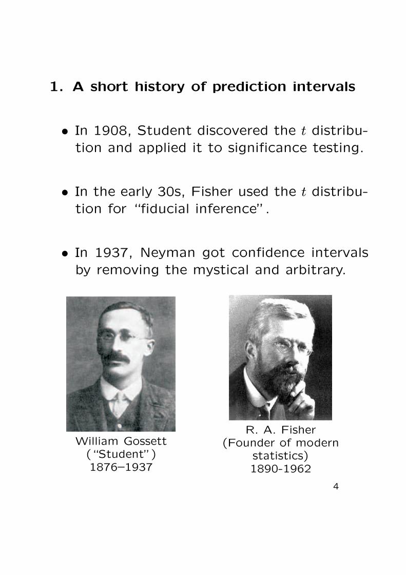
1. A short history of prediction intervals

• In 1908, Student discovered the t distribu-tion and applied it to significance testing.

• In the early 30s, Fisher used the t distribu-tion for “fiducial inference”.

• In 1937, Neyman got confidence intervalsby removing the mystical and arbitrary.

William Gossett(“Student”)1876–1937

R. A. Fisher(Founder of modern

statistics)1890-1962

4

Less often remembered: Fisher also derived

prediction intervals.

• Sample x1, . . . , xn from N (µ, σ).

• Calculate x and s.

• Sample x from N (µ, σ).

• 1933. 1− ε confidence interval for µ:

x± tε/2n−1

s√n

(Because

√n

x− µ

sis t with n− 1 df.

)

• 1935. 1− ε prediction interval for x:

x± tε/2n−1 s

√1 +

1

n

(Because

√n

n + 1

x− x

sis t with n− 1 df.

)

5

Tolerance intervals

After 1940, mathematical statisticians

• went with Neyman,

• emphasized parameters,

• ignored Fisher’s predictive concept.

Inspired by Shewhart’s work on quality control,

Wilks formulated the notion of a tolerance in-

terval. It was studied in the 40s, 50s, and 60s

by Wald, Wolfowitz, Tukey, Fraser, Kemper-

man, and Guttman.

Walter Shewhart(Founder of quality

control)1891–1967

Samuel S. Wilks(Brought statistics to

Princeton)1906–1962

6

Say you are sampling from a distribution P on Z.• You do not know P exactly. You know P ∈ P.• From z1, . . . , zn, you want to predict a new observa-

tion z.• You use a mapping Γ from Zn to subsets of Z.

•Γ is a (δ, ε)-tolerance region if

P n{P [Γ(z1, . . . , zn)] ≥ 1− ε} ≥ 1− δ

for all P ∈ P.

Starting in the late 1950s, Fisher’s idea of a predictioninterval gained a little traction.• He advertised it in his influential 1956 book.• Some attention was paid to a simplified concept

of tolerance region that formalizes and generalizesFisher’s idea:Γ is an (1− δ)-expectation tolerance region if

P n+1{z ∈ Γ(z1, . . . , zn)} ≥ 1− δ

for all P ∈ P.

• Formulas for prediction intervals began to appearin textbooks on regression.

In mathematical statistics, prediction intervals

still receive little attention.

This is occasionally deplored in the pages of

the American Statistician.7

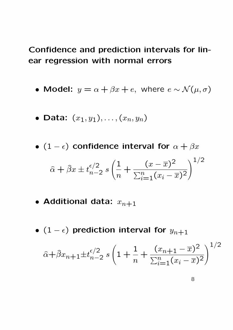
Confidence and prediction intervals for lin-

ear regression with normal errors

• Model: y = α + βx + e, where e ∼ N (µ, σ)

• Data: (x1, y1), . . . , (xn, yn)

• (1− ε) confidence interval for α + βx

α̂ + β̂x± tε/2n−2 s

(1

n+

(x− x)2∑n

i=1(xi − x)2

)1/2

• Additional data: xn+1

• (1− ε) prediction interval for yn+1

α̂+β̂xn+1±tε/2n−2 s

(1 +

1

n+

(xn+1 − x)2∑n

i=1(xi − x)2

)1/2

8

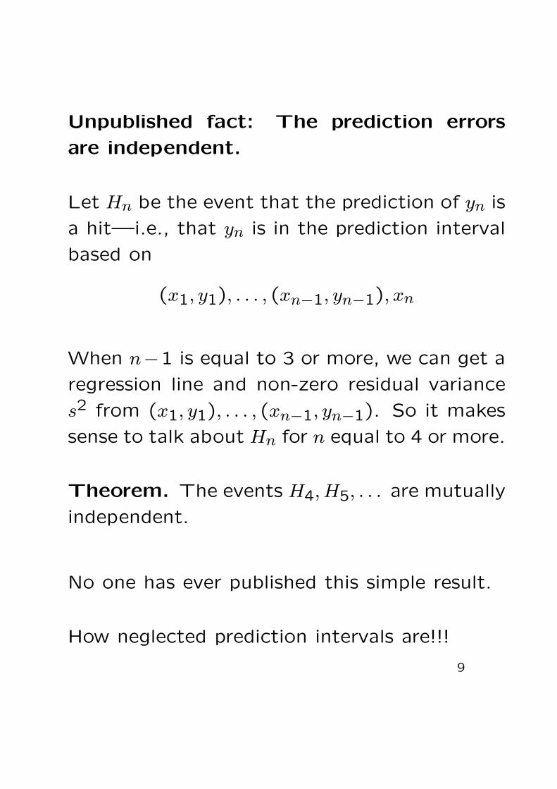
Unpublished fact: The prediction errors

are independent.

Let Hn be the event that the prediction of yn is

a hit—i.e., that yn is in the prediction interval

based on

(x1, y1), . . . , (xn−1, yn−1), xn

When n−1 is equal to 3 or more, we can get a

regression line and non-zero residual variance

s2 from (x1, y1), . . . , (xn−1, yn−1). So it makes

sense to talk about Hn for n equal to 4 or more.

Theorem. The events H4, H5, . . . are mutually

independent.

No one has ever published this simple result.

How neglected prediction intervals are!!!

9

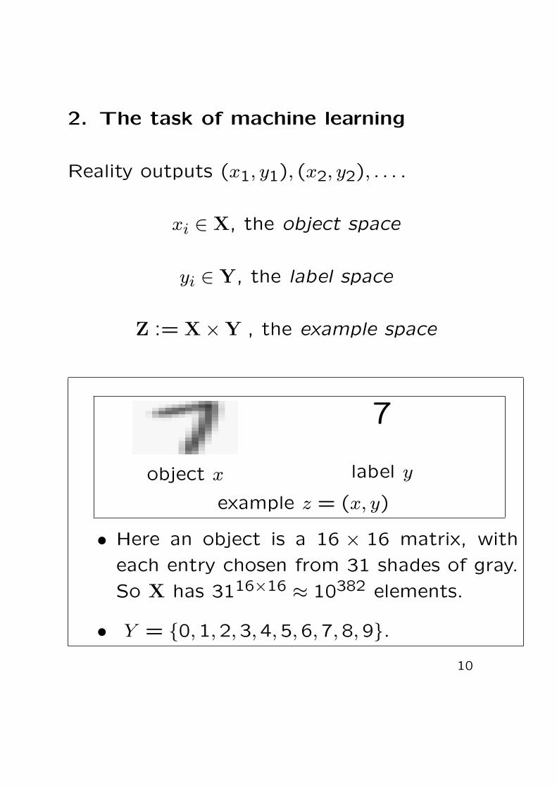
2. The task of machine learning

Reality outputs (x1, y1), (x2, y2), . . . .

xi ∈ X, the object space

yi ∈ Y, the label space

Z := X×Y , the example space

object x

7

label y

example z = (x, y)

• Here an object is a 16 × 16 matrix, with

each entry chosen from 31 shades of gray.

So X has 3116×16 ≈ 10382 elements.

• Y = {0,1,2,3,4,5,6,7,8,9}.10

z1, . . . , zn is the same as (x1, y1), . . . , (x1, yn)

The task: Predict each label after seeing its

object.

• From x1, predict y1.

• From (x1, y1), x2, predict y2.

• From (x1, y1), (x2, y2), x3, predict y3.

• Etc.

Assumption: Randomness.

Reality chooses the examples independently

from some probability distribution Q on Z.

(The zi are independent & identically dis-

tributed.)

No assumptions about Q.

Usually independence can be weakened to ex-

changeability.

11

3. Prediction with confidence

Z = X×Y

Write Z∗ for the set of all finite sequences ofelements of Z:

Z∗ = ∪∞n=0Zn

A level (1−ε) confidence predictor is a mapping

Γ : Z∗ ×X → 2Y.

After observing old examples z1, . . . , zn−1 andthe new object xn, we predict that xn’s labelyn will be in the subset

Γ(z1, . . . , zn−1, xn)

of the label space Y.

Write Hn for the event that this prediction iscorrect, and call Hn. This event is the predic-tor’s hit on the nth round.

12

A (1− ε) confidence predictor is

• exactly valid if its hits are independent and

all happen with probability (1− ε).

• conservatively valid if the probability that

the predictions on rounds n1, . . . , nk are all

hits is always at least (1− ε)k.

(The probability statements must be true no

matter what probability distribution Q on Z

governs the data.)

In our forthcoming book, Vovk, Gammerman,

and I demonstrate the existence of valid confi-

dence predictors and explain how they are con-

structed.

13

Valid confidence predictors are constructed

from nonconformity measures

As Vovk, Gammerman, and I explain, a valid

confidence predictor is obtained from a real-

valued function A on strings of the form

(x1, y1), . . . , (xn−1, yn−1), (x, y).

To get the confidence predictor,

• interpret A((x1, y1), . . . , (xn−1, yn−1), (x, y))

as a measure of how different (x, y) is from

(x1, y1), . . . , (xn−1, yn−1);

• predict values of yn that make (xn, yn) dif-

fer minimally from (x1, y1), . . . , (xn−1, yn−1).

I will explain this more precisely later.

14

Because of the way they are constructed, valid

confidence predictors are called conformal pre-

dictors.

The function A is called a nonconformity mea-

sure.

From a given nonconformity measure, we con-

struct a (1− ε) confidence predictor Γε for ev-

ery ε ∈ [0,1], and they are nested in the natural

way:

Γε1(z1, . . . , zn−1, xn) ⊆ Γε2(z1, . . . , zn−1, xn)

when ε1 ≥ ε2.

The more confident you want to be, the larger

the region.

15

4. Situating conformal prediction in sta-tistical learning theory

Vladimir Vapnik, the founder of statistical learning the-ory, has recently emphasized the distinction between in-duction and transduction.

• Induction: Fix n. Sample z1, . . . , zn. Use

this sample to make a rule for predicting a

new y from a new x.

This rule might be hard wired into devices to beused on many new examples zn+1, . . . , zm, each in-volving a y to be predicted from an x. (Example:give postal workers devices for reading zip codes.)

• Transduction: On each round n, use

z1, . . . , zn and xn+1 to predict yn+1.

Perhaps in the course of making the prediction weformulate a rule for predicting a new y from n ex-amples and a new x, but we do not store this rulefor very long, because on the next round we up-date it to a rule for predicting a new y from n + 1examples and a new x.

16

Induction is more common in practice thantransduction, for two reasons:

• Transduction requires a teacher.

In order the postal worker’s device to update its

algorithm, it must be told the correct digit for each

example that it predicts!

• Until now, estimating confidence for pre-dictions required a batch approach: thehold-out method.

1. Divide the data into two halves — an estimationset z1, . . . , zl and a test set zl+1, . . . , zn.

2. Calculate a prediction rule from the estimationset.

3. Observe the success rate of the prediction ruleon the test set.

4. If the rule works 90% of the time on the testset, give it 90% confidence in future examples.

17

The usual practice in machine learning (PAC,

VC) is to give a rule Γ for forming a prediction

region Γ(z1, . . . , zn−1, xn) ⊆ Y, together with

and a upper bound on the probability that y

will fail to be in the region. One then shows

that this upper bound tends to zero as n →∞.

• The prediction regions often work well in

practice; with reasonable values of n, there

is a very low probability of y not being in

the region.

• But the theoretical upper bounds on this

probability are typically useless (larger than

1) for these reasonable values of n.

Bottom line: Vapnik’s statistical learning the-

ory does not give degrees of confidence. For

this, one must fall back on the naive method

of the hold-out estimate.18

Our new theory of conformal predictors solves the prob-lem of confidence prediction. And the practical perfor-mance of our predictors is as good as those of statisicallearning theory.

But this does not eliminate the need to use inductionrather than transduction when there is no teacher tocorrect each new prediction after it is made. In thesesituations, batch methods must be used, and the hold-out estimate will probably be competitive.

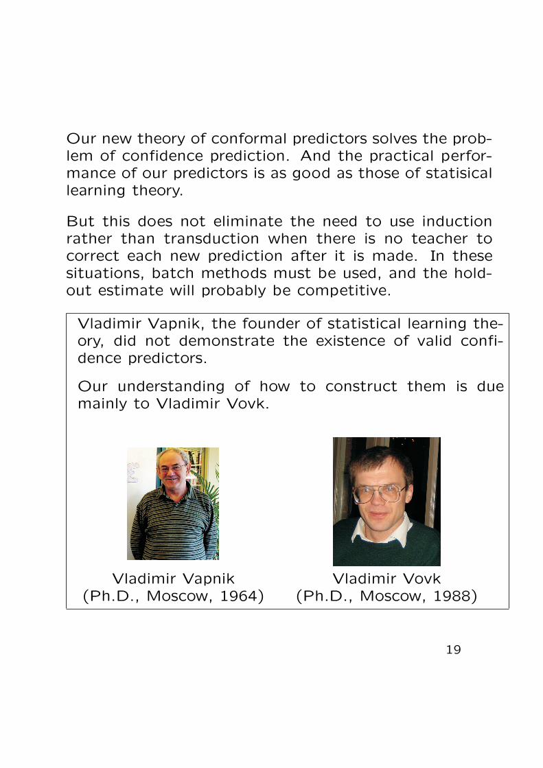
Vladimir Vapnik, the founder of statistical learning the-ory, did not demonstrate the existence of valid confi-dence predictors.

Our understanding of how to construct them is duemainly to Vladimir Vovk.

Vladimir Vapnik(Ph.D., Moscow, 1964)

Vladimir Vovk(Ph.D., Moscow, 1988)

19

5. From a nonconformity measure to a

conformal predictor

Recall that a bag (or multiset) is a collection

of elements in which repetition is allowed.

(A bag is different from a set, because ele-

ments may be repeated. But it is like a set in

that its elements are not ordered.)

Write B for the set of all finite bags of elements

of Z.

Definition: A nonconformity measure is a

function A : B × Z → R.

We interpret A(B, z) as the degree to which z

is strange with respect to the bag B.

Formally, any function A : B × Z → R qualifies as anonconformity measure and can be used in our theory,but in practice we choose A so that a large value ofA(B, z) indicates that z is strange relative to B.

20

As always, Z = X×Y and z = (x, y).

Example: Regression

Suppose X = Y = R. Then a useful noncon-

formity measure is

A(B, z) = |y − α̂− β̂x|,where α̂+ β̂x is the least-squares line based on

the examples in the bag B.

Any other method of obtaining a regression

line can also be used.

Example: Classification

Suppose X = Rk, while Y is finite. Then a

useful nonconformity measure is

A({z1, . . . , zn}, z) :=mini:yi=y d(xi, x)

mini:yi 6=y d(xi, x),

where d is Euclidean distance.

Any other way of scoring a proposed classifca-

tion can also be used.

21

How to construct a 95% confidence region for

yn from• a nonconformity measure A

• old examples z1, . . . , zn−1, and

• a new object xn.

1. Consider separately each y ∈ Y.

2. Let B be the bag consisting of z1, . . . , zn−1

together with (xn, y).

3. For i = 1, . . . , n, let B−i be the bag ob-

tained by removing zi. (For the moment,

(xn, y) will serve as zn.)

4. Set Wi := A(B−i, zi).

5. Set

py :=#{i = 1, . . . , n |Wi ≥ Wn}

n.

Call this the p-value for y. It is the fraction

of the elements in B that are at least as

strange relative to the others as (xn, y).

6. Include y in the confidence region if and

only if py > 0.05.

22

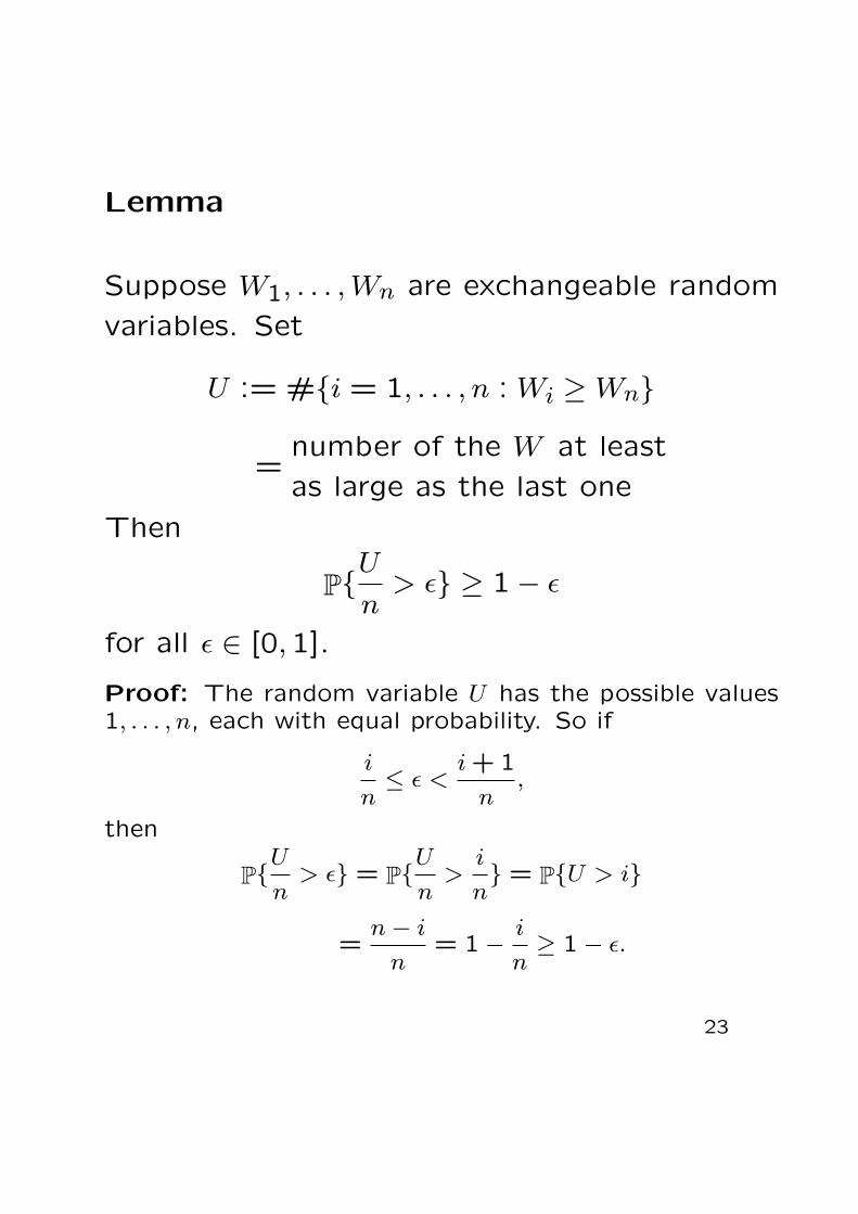
Lemma

Suppose W1, . . . , Wn are exchangeable random

variables. Set

U := #{i = 1, . . . , n : Wi ≥ Wn}

=number of the W at least

as large as the last one

Then

P{Un

> ε} ≥ 1− ε

for all ε ∈ [0,1].

Proof: The random variable U has the possible values1, . . . , n, each with equal probability. So if

i

n≤ ε <

i + 1

n,

then

P{U

n> ε} = P{U

n>

i

n} = P{U > i}

=n− i

n= 1− i

n≥ 1− ε.

23

6. The Generality of the Method

Any method of statistical prediction, together

with any way of measuring its error, produces

a nonconformity measure and therefore a con-

formal predictor:

• Let D be a way of predicting y from a bag

of old examples and a new object x.

• Suppose dist(y1, y2) is some metric on Y.

• Set A(B, (x, y) := dist(D(B, x), y).

The nonconformity approach is universal: Any

method of obtaining valid nested confidence

regions arises from a nonconformity measure.

This is true because the p-values themselves

define a nonconformity measure.

24

If we believe the examples are being generated

by a certain model (Gaussian errors, say), then

we may want to use a nonconformity measure

based on method of prediction that is optimal

for that model (least squares, say).

This will be efficient (the confidence regions

will be small) if the proposed model is right.

It will be valid even if the model is not

right. (We assume only exchangeability.)

25