consortia optimization for european space agency proposals ... · um conjunto de dados de 2013 a...
TRANSCRIPT

UNIVERSIDADE DE LISBOA
FACULDADE DE CIÊNCIAS
DEPARTAMENTO DE ESTATÍSTICA E INVESTIGAÇÃO OPERACIONAL
Consortia optimization for European Space Agency proposals
based on cognitive computing
Izabella Campolina Silva e Hemprich
Mestrado em Matemática Aplicada à Economia e Gestão
Trabalho de Projeto orientado por:
Maria Teresa Alpuim
Alberto Krone-Martins
2019


iii
ABSTRACT
This master thesis intends to study relations between the words written in European Space Agency
(ESA) Invitation to Tender (ITT) abstracts, and, if there is any correlation between the words and
the chance of a certain country to award a bid.
An intermediate task was to compile and organize a proper dataset. A dataset was created using
the ESA Dashboards and ESA Emits from 2013 to 2016 as basis.
Then, we developed the necessary codes to analyze this dataset in R.
We constructed matrices and graphical representations with the relations between Winner
Countries, the ESA Offices and the different ESA Programs. Based on this, our firsts points were
raised and analyzed.
Five countries were selected based in the number of awarded ITTs. They are Germany, France,
Great Britain, Italy and Belgium. These countries were scrutinized using text mining techniques
and statistics models.
Using our dataset, we analyzed the entire text abstract with R packages for text mining, as the TM
package. The original abstracts were organized removing numbers, white spaces and most
frequent words. After these steps, document term matrix (DTM) were constructed. DTM is a
matrix, where the rows are the documents (ITT abstract) and the columns are the variables (most
frequent words). The DTM was the basis for all textual analysis study. Regression models
(logistic regression) were created for these five countries and stepwise methods used for variables
selection. The created models relate words with the chance of a certain country winning an ITT.
The validity of the models was analyzed using statistics parameters as: Sensibility x Specificity
curve (cut-off point), Area under ROC curve, ODD.Ratio and fitted values.
Afterwards, we started to investigate if the ITTs clustered in the DTM defined space. Different
methods were used to define clusters. We verified if clustered formed in the word frequency space
and also in a principal component analysis transformed space. However, results show that no
method results in an automatic clustering using the Silhouette method, suggesting that more
advanced techniques might be needed to extract the true number of clusters. The results of the
application of PCA do not show agglomeration, suggesting internal clustering tendency.
Finally, we can conclude that there seems to exist some relations between words and winner
countries, the reasons for which remains to be studied in further works.
KEY-WORDS: ESA, text mining, R, DTM, logistic regression, stepwise methods, ITT, winner
country, clusters, Kmeans, PCA

iv
RESUMO
Esta tese de mestrado estuda as relações entre as palavras escritas nos resumos dos concursos da Agência Espacial Europeia(ESA - Invitation to Tender - ITT) e, em particular, se existe alguma correlação entre as palavras e a possibilidade de determinado país ser o ganhador do concurso. Um conjunto de dados de 2013 a 2016, com as informações dos dashboards dos status dos concursos e as informações do site Emits fornecidos pela ESA foram organizadas e compiladas. Em seguida, os códigos necessários para analisar esse conjunto de dados foi desenvolvido em R. Construimos matrizes e representações gráficas com as relações entre os países vencedores, os escritórios da ESA e os diferentes programas da ESA. Com base nisso, os primeiros pontos foram levantados e analisados. Em seguida, selecionamos cinco países com base no número de ITTs premiados e representatividade nos escritórios da ESA para desenvolvimento de modelos estatísticos. Esses países são: Alemanha, França, Grã-Bretanha ( Reino Unido), Itália e Bélgica. Com o uso de pacotes de mineração de dados (text mining), com o “TM” do R, os resumos originais foram organizados, de forma a retirar informação irrelevante que poderiam dificultar a realização deste trabalho. Números, espaços em branco e palavras mais freqüentes foram removidas e todo texto foi colocado em minúsculo. Após estas etapas, a matriz documento por termo (DTM) foi construída. Nesta matrix, cada linhas é um documento (neste caso, o resumo de cada um dos ITTs) e cada coluna as variáveis ( neste caso, as palavras mais frequentes na base de dados). A DTM é a base de todo o estudo relativo a análise textual. Para cada um dos cinco países com mais ITTs, modelos logísticos foram criados e métodos de seleção Stepwise aplicados. Os modelos criados relacionam palavras com a possibilidade de um determinado país ganhar um ITT. A validade dos modelos foi analisada utilizando parâmetros estatísticos como: sensibilidade x curva de especificidade (ponto de corte), área curva Roc e Odd. Posteriormente, começamos a investigar se os ITTs se aglomeraram em clusters definidos por estas variáveis. Diferentes métodos foram utilizados. O parâmetro da silhueta foi usado para validação dos clusters, porém os resultados não foram satisfatórios. Aplicou-se a análise de componentes principais (PCA), que permaneceu deixando lacunas, sugerindo que estudos mais avançados devem ser feitos para entender essa questão. Com este estudo, podemos inferir que existem relações entre as palavras escritas nos resumos dos ITTS e a chance de um determinado país ser o vencedor de um determinado ITT. Por essa razão, este tema merece continuar a ser desenvolvido em trabalhos futuros. PALAVRAS-CHAVE: ESA, text mining, R, DTM, logistic regression, stepwise methods, ITT, winner country, clusters, Kmeans, PCA

v
ACKNOWLEDGMENTS
I would like to thank this master’s degree to my mother Sandra and my sister Mariana (Balo) that
supported me, especially in the moments that I wanted to give up.
A special thanks to my husband André for patience and understanding during all this period when
I stayed so far away from our home.
This degree would not have been possible without Professor Teresa Alpuim who, since the first
day in the faculty, gave me all attention, class support and made me love statistics after a “hard” beginning. To Doctor Alberto Krone-Martins, my mentor and friend, that believed that I was able
to do something different.
To Professor António Amorim Barbosa for the incentive.
To my classmate and good friend Felipe Azinheira, who since the beginning helped me in the first
steps of statistics.
To Mr. Stefano Fiorilli and Ms. Ingrid Oppenheimer from European Space Agency (ESA)
procurement department that provided the information necessary for developing this study.
To God that once again, as always, illuminated my way during this journey.
“Os números dominam o mundo”
Platão

vi

7
TABLE OF CONTENTS
ABSTRACT ................................................................................................................................ iii
RESUMO .................................................................................................................................... iv
ACKNOWLEDGMENTS .......................................................................................................... v
LIST OF FIGURES .................................................................................................................... 8
LIST OF TABLES ...................................................................................................................... 9
ABBREVIATIONS ................................................................................................................... 10
INTRODUCTION ..................................................................................................................... 11
I – INITIAL ANALYSIS ........................................................................................................... 12 1. DATASET COMPILATION .......................................................................................................... 12
1.1 Adopted software definition .................................................................................... 13 2. INITIAL DATASET EXPLORATION ..................................................................................... 13 3. TEXT MINING ........................................................................................................................... 23
II - REGRESSION MODELS .................................................................................................. 27
1. OVERVIEW ....................................................................................................................... 27 2. REGRESSION MODEL AND VARIABLES SELECTION METHODS .......................................... 27 3. MODELS COMPARISON AND CHOICE ................................................................................ 30
III - FITTED VALUES, PREDICTION, ROC CURVE AND ODDS RATIO ................... 33
IV – EXPLORATORY CLUSTER ANALYSIS .................................................................... 46
CONCLUSION .......................................................................................................................... 60
REFERENCES .......................................................................................................................... 61
ANNEX....................................................................................................................................... 64

8
LIST OF FIGURES
Figure 1- Countries X ESA_Office (normalization per countries) ............................................. 15
Figure 2- Countries x ESA_Office (normalization per ESA_Office) ......................................... 17
Figure 3- Coutries x ESA programme prPrograms ..................................................................... 21
Figure 4- Suggested data mining flow ........................................................................................ 23
Figure 5- Correlation Matrix of the 60 most frequent words in the DTM extracted from the ESA
ITTs. ............................................................................................................................................ 26
Figure 6-Correlation Matrix- most frequent terms ...................................................................... 26
Figure 7 – Real event x Predicted value ...................................................................................... 37
Figure 8- General representation of a confusion Matrix ............................................................. 38
Figure 9- Germany cut-off point ................................................................................................. 39
Figure 10- Italy Cut-off point ...................................................................................................... 39
Figure 11- Great Britain cut-off point ......................................................................................... 39
Figure 12- Belgium Cut-off point ............................................................................................... 40
Figure 13- France Cut-off point .................................................................................................. 40
Figure 14- ROC curve Belgium .................................................................................................. 41
Figure 15- ROC curve for Germany ........................................................................................... 41
Figure 16- ROC curve for France ............................................................................................... 42
Figure 17- ROC curve for Great Britain ..................................................................................... 42
Figure 18- ROC Curve for Italy .................................................................................................. 42
Figure 19- ODD Ratio for all 5 countries ................................................................................... 44
Figure 20- Hierarchical dendrogram of ESA ITTs. .................................................................... 47
Figure 21- Correlation matrix from all ITT abstracts .................................................................. 49
Figure 22- AGNES clustering ..................................................................................................... 50
Figure 23- Dendrogram of DIANA ............................................................................................. 50
Figure 24- Silhouette value in function of the number of Kmeans clusters ................................ 52
Figure 25- Silhouette value for a range of numbers of PAM clusters ........................................ 52
Figure 26- Cluster- Kmeans ........................................................................................................ 53
Figure 27- Clusters PAM ............................................................................................................ 53
Figure 28 - Kmeans - clusters defined inside others clusters ...................................................... 54
Figure 29- PAM- clusters defined inside other clusters .............................................................. 55
Figure 30- Optimal cluster numbers- PCA.................................................................................. 56
Figure 31- Clustering- Kmeans (PCA) ........................................................................................ 56
Figure 32- kmeans with 24 dimensions ....................................................................................... 59

9
LIST OF TABLES
Table 1 – Matrix with ITT numbers distributed per countries and offices ................................. 14
Table 2- Space sector in Europe and Canada .............................................................................. 20
Table 3- Correlation matrix - most important relations .............................................................. 26
Table 4 – Stepwise forward – Germany ...................................................................................... 33
Table 5- Stepwise forward Belgium ............................................................................................ 33
Table 6- Stepwise forward- Italy ................................................................................................. 34
Table 7 - Stepwise forward- France ............................................................................................ 34
Table 8 - Stepwise forward - Great Britain ................................................................................. 34
Table 9- Prediction x Real event ................................................................................................. 36
Table 10 – Distribution of winner countries per cluster .............................................................. 56
Table 11- Analysis for each component from PCA .................................................................... 58
Table 12- Countries distribution -PCA with 24 dimensions ....................................................... 59

10
ABBREVIATIONS
ESA- European Space Agency
EMITS- Electronic Mail Invitation to Tender System
ITT- Invitation to tender
BE- Belgium
CA- Canada
CH- Switzerland
DE- Germany
DK-Denmark
EE- Estonia
ES- Spain
FI- Finland
FR- France
GB- Great Britain
GR- Greece
IRL- Ireland
IT- Italy
LU- Luxembourg
LV- Latvia
NL- Netherlands
NO- Norway
PL- Poland
PT- Portugal
RO- Romania
RUS- Russia
SE- Sweden
US- United States of America
AUC – Area under a ROC curve
DTM- Document Term Matrix
AIC- Akaike Information Criterion
DF- Degrees of Freedom
AC- Agglomerative coefficient
OD- Odds Ratio
AGNES- Agglomerative Nesting
DIANA- Divisive Analysis
PCA- Principal Component Analysis

11
INTRODUCTION
Invitation to Tender (ITTs) are competitive processes that the European Space Agency (ESA)
organizes to select contractors to develop certain research and development projects related to
several space areas. It is largely through these ITTs, countries bring back the resources invested
in ESA in terms of contracts.
This master project is the first step in the development of a study intending to use machine
learning and statistical tools to find relation between words in Invitation to Tender (ITT) abstracts
and the chance of certain country awarding a European Space Agency (ESA) ITT.
Using from simple to complex text mining techniques as, for example, searching for most frequent
words in ESA Abstracts, this work looks to identify the relationship of certain words with the
probability of a certain country winning a bid. Then, we will try to analyze the clustering of the
documents in terms of words, to look for possible relations between the winning country and
thematic areas.
Summarizing, this study looks to verify the hypothesis that words have relations with the chance
of winning an ESA ITT, for some country. If this is confirmed, bidders’ countries can optimize
their strategies, saving resources, and increasing their probability to make good decisions, already
before starting the proposal organization and proposal partners search.
This subject was developed because, while working in CENTRA-FCUL, in several occasions the
proposal development was started but never submitted. Normally these proposals were from ESA
and a few cases for the PT20201. We gathered one year of proposals and organized them in two
groups: started and submitted proposals and started and not submitted proposals. After dividing
the proposals into these two groups, the author and her collaborators analyzed in detail the
proposals and looked for reasons why they were not submitted. The main reasons were issues
regarding partners or missing technical requirements.
A large amount of resources was lost searching for wrong partners and trying to fit CENTRA
expertise in the ITTs. Considering this problem, we considered interesting to look for alternatives
to improve CENTRA chance of winning ESA bids. And we hypothesized that we could improve
partner selection by performing statistical analysis directly on the call texts.
1 PT2020 – The Partnership Agreement between Portugal and the European Commission, labelled as 'Portugal 2020', acknowledges and underlines the role of R&I policy in promoting the country’s competitiveness and internationalization. https://rio.jrc.ec.europa.eu/en/library/portugal-2020-partnership-agreement

12
I – INITIAL ANALYSIS
1. Dataset compilation
The first challenge was to find available data, without problem with confidentiality, and in
CENTRA expertise field. After a long time searching for a solution, the author remembered that
ESA (our main client), provided information regarding ITTs status (e.g. awarded, re-issued,
evaluated, canceled), in the dashboards monthly sent. Added to this fact, information regarding
abstract, budget, responsibility, country, and others were publicly available at the EMITS
(Electronic Mail Invitation to Tender System) website.
With the dataset defined, we started looking for all the correct information to guarantee the
reliability of this study. We contacted the ESA Procurement Department, responsible for ESA
Dashboards, and explained to them our study. They provided all the necessary information that is
in public domain.
This work was developed using data from the monthly ESA dashboards.
We collected data from 2013 until 2016. The data used was based on three main sources, namely:
• 25 (twenty-five) tables from 2013- 2014;
• 17 (seventeen) tables from 2015;
• And 13 (thirteen) tables from 2016.
After organizing a file with all the awarded ITT, we were able to gather a dataset with 757
observations. With all these Awarded ITTs organized, a unique dataset, including all the
information from EMITS web site, was constructed. The final table contains 17 (seventeen)
columns, representing 17 variables, namely: ESA Site, ESA reference number, Program Name,
ITT Title, Program reference, budget, open date, closing date, countries allowed to participate in
the ITT, price range, directorate name, department name, division name, responsible person,
abstract, winner, country winner.
All these variables are available in the dataset, but it does not mean that all of them were used in
the present work. Only the relevant information for the hypothesis of this thesis were used,
namely: ITT abstract, ESA Office, Country winner and ESA Program.
Before going on with the description of the study, some remarks about the data are relevant:
• The dataset has information regarding only the prime contractor for each ITT,
although other countries could have some participation this information is not
available (this proves to be challenging for Portugal, as it is usually only a partner
in proposals from larger countries).
• All the ITTs awarded to the UK (United Kingdom) were registered as having the
contractor GB (Great Britain).
• ESA has non-European participants in the ITTs, as it is the case of Canada (CA),
United States of America (US) and Russia (RUS).
• A given ITT can appear in multiple monthly Dashboards. The information
regarding ITT awards, was considered in the last version that it appeared. If some
changes occurred between ESA dashboards revisions, these were not considered
relevant.
• There are ITTs with more than one winner country, and that explains why the
sum of Awarded ITTs is larger than the number of observations.
• ITTs that did not have any awarded winner where left outside this study.
• Missing information was completed as not applicable.

13
• In this dataset there are only 5 (five) different ESA Offices, although there are
other offices, that do not make part of this study. Here, we considered public data
from ITTs that were published and awarded. Each office has a different focus,
which is as follows:
1. ESA's headquarters (HQ)2 are in Paris where policies and programmes
are decided. ESA also has sites in other European countries, each of
which has different responsibilities:
2. ESOC3, the European Space Operations Centre in Darmstadt, Germany;
3. ESRIN4, the ESA Centre for Earth Observation, in Frascati, near Rome,
Italy;
4. ESTEC5, the European Space Research and Technology Centre,
Noordwijk, in the Netherlands.
5. ECSAT6, the European Centre for Space Applications and
Telecommunications, Harwell, Oxfordshire, United Kingdom.
1.1 Adopted software definition
Initial tables received from ESA where in Excel, but Excel lacks many statistical analysis features,
besides slowing down significantly for larger data volumes. Thus we decided to adopted another
environment more adapted to this study. The software chosen was R7.
R is a free software environment for statistical computing and graphics, with many tools for text
mining, statistics analysis, regression analysis, data analysis and many more other functionalities.
There is a unified repository, where all new packages and releases are organized and available.
This repository, CRAN8, is the official source of all R packages and releases. Everything is
accessible in the Internet so it can be easily spread and used around the world, besides encouraging
scientific reproducibility. Since it has so many users, the software gets updated and more powerful
every day. This software has a great feature which is that every programmer around the world can
work in the development of R package tools. Also, there is a huge number of online forums. Users
working together in the same tool make possible to discuss ideas and solutions while you are
programming.
All the codes in this work were developed in R. This choice makes possible future uses and
evolution of the developed tools and analysis, without extra resource expenses in infrastructure
and licenses. Although we focused in ESA ITTs, this code can be used to get results regarding
text mining and clustering for other types of tenders.
2. Initial dataset exploration
The original dataset format was in Excel. After the entire dataset compilation that we performed
in Excel, we exclusively adopted R to further manipulate and analyze the data. Regarding our first
challenge, it was necessary to use two R packages: XLConnect and Stringr. XLConnect is R
2 HQ - https://www.esa.int/About_Us/Welcome_to_ESA/What_is_ESA 3 ESOC – https://www.esa.int/About_Us/Welcome_to_ESA/What_is_ESA 4 ESRIN – https://www.esa.int/About_Us/Welcome_to_ESA/What_is_ESA 5 ESTEC – https://www.esa.int/About_Us/Welcome_to_ESA/What_is_ESA 6 ECSAT - https://www.esa.int/About_Us/Welcome_to_ESA/What_is_ESA 7 https://www.r-project.org/ 8 https://cran.r-project.org/

14
package for manipulating Microsoft Excel files from within R [1], and we used this package to
be able to read the data within R. Stringr is an useful package for string and character
manipulation, whitespace tools, locale sensitive operations and pattern matching operations [2],
and it was used to perform the text manipulation on our dataset once it was in R.
To complete manipulate all the initial data and extract the information regarding the country from
which the winner entity was, from the original dataset, we used one code also adopted by editors
for text modification, the so-called regular expressions.
A regular expression, regex or regexp is a sequence of characters defining search pattern.
Normally this pattern is used by string searching algorithms to "find" or "find and replace"
operations on strings, or for input validation [3].
With the use of all packages listed above and regular expressions, it was possible to separate from
the initial text, the information regarding the winner ITTs country. After this, the dataset was
organized with all the information necessary to develop the proposed study. The final dataset had
17 columns. The original dataset included 16 variables and the 17th variable was created to register
the winner countries.
One last procedure was necessary before starting building graphics: normalization of the dataset.
In statistics, normalization means adjusting values measured on different scales to a common
scale, often prior to averaging. In other words, using this procedure is possible to have the data in
the same pattern. This guarantee that, the information is under the same assumptions and scale.
According to R.Hogg et al., “A very useful family of probability distributions is the normal
distribution [4] which has shown to fit well to many observed variables in practice”.
This happens, very often, because sums and averages of quantitites are approximately normally
distributed as a consequence of the Central Limit Theorem and its generalizations.
The central limit theorem (CLT), implies that under most distributions, normal or non-normal,
the sampling distribution of the sample mean will approach normality as the sample size increases
[5].
In statistical analysis, it is often assumed that the population from which a sample was taken is
normally distributed, symbolically, N ( 2) [6], where stands for the mean value of the
population and 2 represents its variance.
In this case, the definition normalization is more related the necessity to organize the data in same
pattern.
Using R, a matrix was created, where columns represent one country and lines one ESA Office:
Table 1 – Matrix with ITT numbers distributed per countries and offices
This matrix represents the data used to create the reference for each represented relation in those
graphics (except, graphic of ESA Programs)
Three graphics were plotted and for each one of then, data was organized using different
references, as follow:
With data and the final dataset organized, it was possible to perform the first visual exploration
by creating graphics that show the relations of the dataset columns. For such graphics, we use the
following color encoding:

15
• Green color - no correlation between variables
• White color - correlations between variables is perfect.
The color scale starts at green color (no correlation) and finishes in white color (100%
correlation). The lighter the color scale, the stronger the correlation between variables. The main
objective of these graphics is to see the behavior of the relationships between ESA ITTs, Winner
Countries and ESA Programs.
ITTs distribution considering normalization (reference) per countries:
We start by exploring the relation between the ESA centers and the countries winning ITTS.
The ratio por each relation is:
ITT number per country in certain office
ITT total number per country
From this, a visual representation of the matrix was created, considering winning Countries versus
the ESA Office awarding the ITT. This is shown in Figure 1. As the proportion is performed per
country, it is possible to verify how ESA Offices behave regarding the countries.
The information obtained here shows how ITTs distribute among countries considering each ESA
Offices. It is possible to see that all countries have more ITTs awarded by ESTEC than by any
other ESA office.
This happens because the total number of observations is larger in ESTEC than in other offices,
and because ESTEC is a much more diverse center, awarding ITTs for different areas.
However, there are further points to be raised from this matrix visualization:
• ESTEC is ESA's central Space Research and Technology Centre. Considering its broad
research areas (everything that goes into a satellite), it is reasonable that this center has a
huge number of ITTs awarded. Considering the ESTEC behavior towards different
countries, it is expectable that they have business with almost all countries.
Figure 1- Countries X ESA_Office (normalization per countries)

16
• Countries as GR (Greece), LV (Latvia) and US (United States of America), have a 100%
awarded ITTs in ESTEC. It does not mean they did not submit ITTs in other offices, but
they won just in ESTEC.
• ESRIN has a 100% correlation with Estonia (EE). That happened because Estonia has
awarded ITTs only in ESRIN., indicating that they might favor Earth Observation.
• HQ has a 100% correlation with Russia (RUS). That happened because Russia has
awarded ITTs only in HQ, indicating more sensitive negotiations
• ESOC does a lot of business with Romania (RO), comparing with other countries. We
can consider Romania as an outlier in this case. Starting in 22 December 2011, Romania
became the 19th Member State of the European Space Agency.
The first agreement between Romania and the European Space Agency (ESA) was signed
in 1992, followed in 1999 by the Romania-ESA Agreement on cooperation in the
peaceful exploration and use of space. Starting in 2007, Romania contributed to the ESA
budget as a European Cooperating State (PECS), status ratified by Law no. 1/2007[7].
This summary shows that this outlier, in fact, has made efforts in space operation since a
long time ago. Romania has her own organized Space Agency (ROSA- Romania Space
Agency). Romania shows a great interest in Space Operations and probably developed
good proposals for ESA. Regarding all the other offices, Romania awarded 14 ITTs
during the period in study: 7 at ESOC, 3 at ESRIN and 4 at ESTEC. It is possible to
confirm that Romania also has weaker correlations with ESRIN and a stronger correlation
with ESTEC.
• All ESA Offices do business with Switzerland (CH). This can be justified because,
Switzerland has a strong space office that supports Swiss bidders preparing the proposals,
budget and partners search. The Swiss Space Center works closely together with the
technology transfer office of ETH Zurich. The ETH technology transfer supports the ETH
community in a broad range of intellectual property matters including the contractual
negotiations with ESA that follow any submitted proposal/tender accepted by ESA [8].
• Czech Republic (CZ) has a good correlation with ESTEC and ESRIN.
• Poland (PL) has a good correlation with ESTEC, ESRIN and ESOC.
• Portugal (PT) has a small correlation with HQ and ESRIN and a little stronger correlation
with ESTEC. Portugal has no awarded ITTs by ESOC and ECSAT (as prime contractor).
Portugal has a very recent Space Agency, that until very recently was still under
construction [9]. Other considerations that can be taken are:
1. Portugal has no ITT awarded in the following areas: Space Applications and
Telecommunications (ECSAT) and in Space Operations (ESOC). Probably,
Portugal has not enough expertise or organized research & development in such
areas.
2. Portugal might lack a good network with the players of those areas and offices.
Thus, a good opportunity for Portugal could be (after point 1 above is addressed)
to contact Space Agencies and National delegations of other countries having
high correlations with ESA Offices where Portugal has no business, namely,
ECSAT and ESOC, looking to form partner clusters.
3. One possible delegation to be contacted to reinforce relations could be Romania.
Romania is a small country, relatively new in ESA and in the European Union
[10]. The starting point might be to negotiate collaborations in ESOC, with whom
the Romanians have a good correlation. This kind of deal could be fruitful for
both countries and open new expertise areas in Portugal.

17
ITTs distribution considering normalization (reference) per ESA Offices:
The second relation we explored was considering the normalization per ESA Office.
The ratio por each relation is:
ITT number per country in certain office
ITT total number per office
The information shows ITTs distributions, considering the relation between the countries and
ESA Offices. The question is: which office do the countries work with?
It is possible to see that most countries have a sparse relationship with the ESA Offices. Only
Belgium, Germany and Italy have contracts in all ESA Offices. Probably, they have enough
expertise in many areas that fits in ESA necessities.
Figure 2- Countries x ESA_Office (normalization per ESA_Office)
• Belgium (BE) works with all offices. Belgium is the heart of many world organizations,
e.g. NATO (North Atlantic Treaty Organization) [11]. Other relevant point is that ESA
has an office in Brussels [12]. Considering this quick insight, we might say that Brussels
is politically central to every important happening in ESA and in Europe.
• Canada (CA) works with ESRIN, what makes sense since Earth Observation is one of
Canadian major space focus areas. Canada has many satellites developed and under
development with ESA for essential information on ocean, ice, land environment, and the
atmosphere [13].
• Spain (ES) works with almost all ESA Offices. Considering that the Spanish have actions
to include space knowledge since the elementary school, it is not strange to see the
number of business they have with ESA. ESA has in Spain a European Space Education
Resource Office (ESERO).
“ESERO is an ESA education initiative providing qualified teacher training and dedicated
curricular classroom resources and activities, using space to enable Spanish primary and
secondary school teachers to inspire their pupils in STEM (Science, Technology,
Engineering and Mathematics), trigger their natural interest and curiosity about the world

18
around them, stimulate the acquisition of scientific know-how and methodology, and help
them develop the critical thinking they need to master their own future.
ESA’s new ESERO office in Spain was formally inaugurated in Granada, October 2017.
Hosted at Parque de las Ciencias, ESERO Spain joins the existing ESA ESERO network,
which, for over a decade, has acted Europe-wide in support of national school education
systems with innovative science teaching and learning strategies that use space as a
context” [14].
• Germany (DE) works with all ESA Offices. Germany has its own space agency DLR-
Deutsches Zentrum für Luft und Raumfahrt [15]. The major German efforts are in ESOC.
This is natural once ESOC is in Darmstadt, Germany, however it might indicate location
bias for contracts.
Added to this fact, it is relevant to point out that DLR has 24 research institutes from
many expertise fields, such as: Space Propulsion, Space Systems, Space Operations and
Astronaut Training [16]. This huge number of research institutes suggests that Germany
has a huge quantity of specialized researchers studying many different fields. Germany
may bid in a lot of ESA ITTs from many different research branches. More proposals
submitted also naturally results in more chance of winning at least a proposal.
• Italy (IT) works with all ESA Offices. The Italians have their own space agency.
Considering this, they developed through the years expertise in many different areas in
Space Sector, and with great chances to do business with ESA. Italians work together
with ESA in many missions [17].
• Portugal has business with ESTEC, ESRIN and HQ. One possible reason for Portugal not
to have awarded ITTs in other offices is: lack of expertise or even lack of partners. In
this case, Portugal should improve its participation in other offices, contacting national
delegations that do business with ESOC and ECSAT for productive collaborations. Good
options could be Romania (as we identified in the previous section) or Poland. These
countries normally fit in an ESA special programs under geo returns. This Industrial
Policy and Geographical Distribution play an important role in ESA procurements. One
of the main elements, in ESA's Industrial Policy, is the set of rules relating to geographical
distribution or fair return [18].
Another possibility is that Portugal should contact delegations of countries as Germany,
Italy and Switzerland. Those countries have business with all ESA offices, and possibly
expertise that is missing in Portugal, and those are necessary to improve Portuguese Space
Sector and relevance in an ESA context.
• Switzerland has business with all ESA Offices, except ESRIN. This is expectable, once
Switzerland has big companies for Space sector, as Ruag Space.[19]
• France (FR) and Great Britain (GB) do business with 4 ESA Offices (ESOC, ESTEC,
ESRIN and HQ). These countries have a good relationship with those offices. France has
her own Space Agency CNES [20] that is the largest budget contributors to ESA, besides
being a major partner in launch services from Arianespace, as it is also the case of Great
Britain [21].
An additional study was done to verify if the countries with more awarded ITTs had more
institutions and investment dedicated to space field, e.g., space office with dedicated professional
staff or a complete space agency.

19
Considering all the points raised regarding the two plotted graphics, one hypothesis was raised:
is there any relation between the number of ITTs awarded and the number of employees dedicated
to space sector?
To answer to this question a research comprising extensive search in the Internet and contacts
with Space Agencies and National Space Offices was done. Information regarding space agencies
and space offices in Europe and Canada was collected. All data we found in the internet and that
were provided by space agencies and space offices is organized in Table 1.
This table summarizes all the information that was sent by agencies and space offices around
Europe and Canada.
As shown, many countries did not answer the question about the number of employees, but
countries with more awarded ITTs sent the information (except GB and BE). The country with
more employees is Germany with 8.127. Italy has 237 employees. France in 2017, hired 98 new
employees. All documents related to these numbers are attached in final part of this study.
Considering the number of employees, it is easy to conclude that Germany wins more, but also
has more employees directly paid by space-oriented budget in the Space Area.
Poland does not have a lot of participation in ESA but considering that they just exchanged
Accession Agreements to ESA in September 2012 and already have a space agency with 48
employees, we can expect Poland to have a relevant participation in ESA ITTs.
Spain is not among the 5 players chosen for this study. They have 1200 employees dedicated to
space sector technical issues. Regarding their efforts, we can expect Spain in a continuous
growing number of ITT awarded.
Italy has less employees than Spain, but more awarded ITTs. This is in direct relation to the
investment from Italy in ESA, that is the third major contributor to ESA budget, with more than
two times the investment from Spain.

20
Table 2- Space sector in Europe and Canada
ITTs normalization (reference) per ESA_Programs
Using the same dataset (with only the information regarding the ITTs awarded), it was possible
to make another analysis considering how the ESA Programs were distributed per countries.
ESA Programs are a way that ESA “solves issues”. Normally, ESA creates a program that will
have a lot of associated projects for solving a bigger issue.
In this case, the normalization was made considering the total number of ITTs divided per
Programs name per country. The ratio por each relation is:
ITT number per country in certain program
ITT total number per program
Space
Office
Space
AgencyCountry Final action status Answered?
x Romania Email sent 14/10/18 No
x Belgium [email protected] No
x Switzerland Form sent by internet 14/10/18 No
x Canada 14-10-2018 - by form internet YES- 670 employees ( answered 24-10-18)
x Italy 14-10-2018 ([email protected]) YES - 16-10-2018 ( 237 employees)
x France 14-10-2018 - by form internet YES- 23/10/18 ( report annual in french)
x UK 14-10-2018 - [email protected] No
x PT 14-10-2018 [email protected]. No
x CZ 15- 10-2018 [email protected] No
x DK 15- 10-2018 [email protected] YES - 17/10/2018 ( 150 employees)
x EE 15- 10-2018 - [email protected] YES - 15-10-2018 ( 2 employees)
x FI 15- 10-2018 - kimmo.kanto@ businessfinland.fi No
x GR 15- 10-2018 - internet form No
x LUX 15/10/2018 - [email protected] No
x LV 15/10/2018 - [email protected] No
x NO 15/10/2018 - [email protected] No
15- 10-2018 -www.space-ireland.ie No space agency - but 5 persons working to space
15- 10-2018 - Michaela Gitsch
[email protected] - 13 employees
14-10-2018 - by form internet . Another form sent 26/10/18
( https://www.dlr.de/rd/desktopdefault.aspx/tabid-2096/). Form
answered in 26/10/2018)
Yes -here are the figures (as of September 2017):
Total number of employees: 8.127 (2.587 female)
Non-scientific staf
f: 3.404 (50.7 % female)
Scientific staff: 4.723 (18.2 % female)
Average age: 40 years
PhD candidates: 969
Trainees: 237
Student interns: 440
14-10-2018 - [email protected]
YES-26/10/18 -
Around 2000 employees, 1200 of them dedicated to
direct scientific- technical activities
14-10-2018 - [email protected] Answer received 17/10/18 - 48 employees
x IRL
x ES
x PL
x AT
x Germany

21
• It confirmed that countries having a good correlation with almost all ESA Offices
(Germany, Italy, France, Great Britain), have a NEGATIVE correlation with each other.
In other words, for example, in ESA programmes that Germany wins, the other 3 major
countries (Great Britain, France and Italy) have almost no ITT awarded.
When one big player wins, another big player is out, and they complete each other. If it
was possible to compile all those ITTs considering them as just a single country they
would be in almost every ESA program.
• Portugal (PT) has a small participation as prime for ESA Programs. It is possible to say
that Portugal has an irrelevant participation in ESA programs when we consider all ESA
Members. Portugal awarded 17 ITTs as prime contractor in 757 observations. This is also
expected given the very small investment from Portugal in ESA (0.4% of the annual
budget for 2019). Small countries as Romania, Czech Republic and Poland have stronger
correlations than Portugal with a given ESA program.
• Belgium (BE) could be called the fifth country in awarded ITTs. Belgium has a negative
correlation with the big four countries. It means that Belgium works in Programs that
Figure 3- Coutries x ESA programme
prPrograms

22
Germany, Italy, France, Great Britain normally do not have a lot of participation, almost
as if it was avoiding the major countries
If we could put together the 5 countries Germany, France, Great Britain, Italy and
Belgium, as one, it would be winning around 76% of the ESA ITTs (575 of 757
observations).
• In the graphic it is possible to verify a lot of white cells indicating a perfect correlation
between the country and ESA Program. This is not difficult to happen. There are many
programs dedicated to specific countries which do not allow the participation of other
countries. ESA can create one ITT considering special needs and interests from a certain
country. In the database, it is possible to find special dedicated programs to Romania
(RO), Poland (PL) and Czech Republic (CZ).
Comparison of the three graphics analyzed above:
In the first graphic it was possible to analyze how ESA Offices behaves with countries (who/how
ESA Offices contract). In the second, it was examined how countries distribute their efforts
among ESA Offices. In the third and last graphic, it was possible to identify how the ESA
programs are distributed among countries.
Considering all the relevant points observed, it might suggest that:
• Countries with well-defined interests, normally represented by a local Space Agency,
have more ITTs awarded, capillarity among ESA Offices and more flexibility to work
with different ESA programs.
• Small countries with a Space Agency can have an important participation in focused ESA
ITTs (e.g. Romania)
• Countries with no Space Program defined by a Space Agency or Space Office become
less important as prime contractors.
• Regarding the huge concentration of ITTs in 5 countries, Belgium, Germany, France,
Italy and Great Britain, it is possible to say that other countries work only with the ITTs
that were not relevant for countries with a defined space strategy and good know-how in
specific areas.
• Small countries such as Ireland, Portugal, Poland and Romania have sparse correlation
with all the ESA Offices, except ECSAT. This fact could suggest that those countries
could cluster together and join forces to have more participation in ESA ITTs.
• Using the information provided by these three graphics, every country involved in this
study can at least “see clearly” what are their strengths and how they should improve their
efforts to win more ESA ITT.
These firsts results were possible using the relations between the number of ITTs per countries,
offices, and programs.
From now, another type of study will be developed: text analysis relating words in ITT abstract
with the chance of certain country wins an ESA ITT.
Text mining techniques will be used to “clean” the dataset from “useless” information and prepare
it for the models and cluster analysis.
This next part will be developed considering only the five countries with more awarded ITTs in
this dataset. For them, models and analysis will be made.

23
3. Text mining
One of the major focus of this thesis was the capacity to work with text.
According to Ronen Feldman & James Sanger, "Text mining is a technique that tries to solve
issues regarding overload information using, data mining techniques natural language processing
(NLP)9, information retrieval (IR), and knowledge management.
According Ronen Feldman & James Sanger, “Text mining uses document collections pre-
processing (text categorization, information and term extraction), intermediate representations
storage, and analysis, and results visualization”. [22]
Normally, relevant information is hidden inside a huge number of paragraphs and words that
requires the correct preparation to reveal this information. This is what usually is called
unstructured data. This analysis task becomes more complex when there is a huge number of
documents to be analyzed.
According to Tandel et al., [2019] “Text mining examines in detail text in natural language and
then lexical patterns are detected to extract important information”. The usual necessary steps to organize unstructured and messy data are presented in figure 4 [24].
Figure 4- Suggested data mining flow
There are different ways to store text in text mining approaches. Until now, our database was
manipulated using R tools for string and character extraction. Here text will be manipulated in a
way that makes possible to clearly quantify the information hidden inside the characters and
strings.
Text is usually stored as strings (i.e., character vectors) within R, and often text data is first read
into memory in this form. But another way, better to perform analysis, is a Corpus.
“A Corpus is a type of object that contains raw strings annotated with additional metadata and
details “.[25]
There are special packages in R for text manipulation. In this study we mostly used the TM
package.
The text information basis of this study is the Abstract column from ESA ITTs. Tools were used
for the following tasks:
• StemDocument - to maintain the main word root;
• Tolower - to convert the text in lower case. “R” is Case sensitive, and it is completely
mandatory to put all the text in lower case to avoid the same word recognized twice, one
in lowercase and other with uppercase;
• Stopword - to remove meaningless words like, a, an, the.
• RemoveWords - to remove selected words. In this case, words that appeared more than
300 times were removed from the database. Words that are ordinary, with many
repetitions do not contain relevant information.
• StripWhitespace - to remove extra white spaces.
9 Natural language processing (NLP) is a subfield of computer science, information engineering, and artificial intelligence concerned with the interactions between computers and human (natural) languages,

24
• RemoveNumbers - to remove numbers from the text.
• WordStem - This function extracts the stems of each of the given words in the vector.
After these steps, the dataset is ready to become a Corpus to generate a document term matrix
(DTM). According to K. Welbers et al., “Document term matrix (DTM) is one of the most
common formats for representing a text corpus (i.e. a collection of texts) in a bag-of-words
format”.
The DTM is a matrix where rows are documents and columns are the variables (in this case, the
most frequent words). Each cell indicates the frequency each term or variable appears in the
document. Using this representation is easier to analyze vector and matrix, as number, not text.
Added to this, DTM format is more memory efficient and allows the analysis with optimized
operations. Two of the most established text analysis packages in R that provide dedicated DTM
classes are TM and Quanteda”.[26]
After applying the afore mentioned tools (StemDocument, Tolower, Stopword, RemoveWords,
StripWhitespace, RemoveNumbers and WordStem) to all dataset, we selected the most frequent
words, those that appeared more than 300 times in the dataset, in a first step.
Those words are:
"activ","also", "base", "can", "current", "develop","esa", "high", "includ","level", “new",
"oper" , "perform", "process", "provid", "requir", "satellit”, “servic","shall", "space", "support"
"system", "technolog", "use" , "data", "design", "implement", "stud", "test", "mission”, "procur",
"model", "need" ,"object", "addit","inform","measur","smes","will", "phase"
A second step was performed to remove those words from our documents and define the final
DTM. The data is then ready to have the sparsest terms removed, and words that appears in 85%
of the documents kept. Finally, we found our relevant terms (words). We have 60 words with
maximum length of 10 characters, and the data characteristics are:
<<TermDocumentMatrix (terms: 60, documents: 757)>> Non-/sparse entries: 9497/35923 Sparsity : 79% Maximal term length: 10 Weighting : term frequency (tf) The definition of the word’s frequency cut point has a relevant role in DTM definition. For example, the same procedure for a new DTM was done. First, the code for “Most Frequent Word” was compiled for words with frequency of 250 times. The number of words increased from 40 words to 50 words, namely, "activ","also","applic","base","can","current","develop","differ","esa","ground","high","includ
","level","new","oper","perform","process","propos","provid","requir","satellit", "servic",
"shall",
"space","support","system","technolog",”use","data","design","implement","power","product","studi","test","futur","mission","procur","entiti","model","need","object","programm",”addit","inform","measur","pleas","smes","will","phase".
In this example, the final DTM has a smaller number of terms: <<TermDocumentMatrix (terms: 51, documents: 757)>> Non-/sparse entries: 7824/30783 Sparsity : 80% Maximal term length: 10

25
Weighting : term frequency (tf) This other simulation was done to demonstrate that the parameter defined by the user can impact the models. In this study, our final selection was to remove words that appeared 300 times. One possible way to find relationships between variables is using a correlation matrix, that can
be easily visualized in R using the corrplot package.
According to David Shen & Zazai Lu, in 2006 a correlation is a measure of the strength of linear
relationship between random variables. The population correlation between two variables X and
Y is defined as
ρ (X, Y) =
cov( X ,Y )
Var( X )Var(Y )
The parameter ρ is called the product moment correlation coefficient or simply the correlation
coefficient.
This number summarizes the linear relation, considering the direction and closeness between two
variables. The sample value is called r, and the population value is called ρ (rho). The correlation coefficient can take values from -1 to +1. The sign (+ or -) of the correlation defines the direction
of the relationship. When the correlation is positive (r > 0), it means that as the value of one
variable increases, so does the other.[27]
We created such a matrix to reveal how the 60 most frequent words are related. This is
represented in Figure 5. When the color becomes darker and the points are becoming bigger a
stronger relation exists between the variables that are in coordinate X x Y. Using this tool, it is
easy to identify words that appear together.

26
Finally, in Table 3, the most relevant relations appearing in the correlation matrix are represented.
Again, the scale of blue, from light to dark, was used to define how strong is the relation.
Figure 6-Correlation Matrix- most frequent terms
contractor entiti program activit emits full incl industrial news nonprimes pleas activity polici policy restrict nonprim
contractor o o o o o o o o o o o o o
entiti o o o o o o o o o o o o o
program o o o o o o o o o o o o o
activit o o o o o o o o o o o o o
emits o o o o o o o o o o o o o
incl o o o o o o o o o o o o o
industrial o o o o o o o o o o o o o
news o o o o o o o o o o o o o
nonprimes o o o o o o o o o o o o o
pleas o o o o o o o o o o o o o o o
polici o o o o o o o o o o o o o
restrict o o o o o o o o o o o o o
noprim o o o o o o o o o o o o o
Table 3- Correlation matrix - most important relations
Figure 5- Correlation Matrix of the 60 most frequent words in the DTM extracted from the ESA ITTs.

27
II - REGRESSION MODELS
1. Overview
One of the firsts visual exploration of the database we constructed in this study showed the
distribution of ESA ITTs awarded in a Countries versus ESA Programs matrix (Figure 3).
It was possible to conclude from this analysis that 5 (five) countries had more ESA Programs
participation than others. These five countries are: Belgium (BE), France (FR), Germany (DE),
Great Britain (GB) and Italy (IT). They together appeared 575 times in 757 ITTs observed.
Considering this, without any further information, it is possible to infer that when ESA announces
one ITT one of these countries have a possibility of winning around 575/757 (76%) as prime
contractors. To study if it would be possible to predict the chance of each one of these countries
to win an ITT based on the words written in the ITT abstract, we study then the development of
statistical models using the 60 variables selected in the previous chapter as parameters.
2. Regression model and variables selection methods
In this work we explored Logistic Regression models and variables selection methods, as
Stepwise Forward, Stepwise backward and Stepwise both (hybrid).
In the first chapter were defined the variables to be used in the models: 60 words that appear in
85% of the documents and have some relation between each other, as confirmed by the
Correlation Matrix (Figure 5). Most relevant relations were represented in Table 3. Now, we focus
in searching to build models that relate abstract words with the chance of certain country winning
an ITT.
For example, the logistic regression is done between the most frequent terms and the frequency
of them in each abstract from awarded ITT. The most frequent terms were observed if appeared
or not in the awarded ITT. Terms were identified to a coefficient and included in a model.
In the end, the models will answer the principal point of this study: Which words should be in the
ITT abstract to indicate that a certain country has more chance of winning?
The models will relate language terms that guarantee that the chance of success is not random10,
and the fact that they appear in an ITT, increase the chance of success of a certain country in the
ESA tender.
We developed an individual model for each. As there are 5 countries and 4 models per country,
20 models were developed.
Before discussing the development of the models, it is necessary to understand the basic concepts
of regression.
According to R. Hogg et al. [2015], “Regression is a technique that explains the result of some
process in terms of some associated (explanatory) variables by means of a mathematical model”.
Models are created to estimate variable response , when explanatory variable values are know If
, there is an idea to create an equation that relate these variables, it is possible to say that we can
“fit” the model to the data[28] and try to guess the future, or predict the response. There are several
types of regression but the one that will be used in this work is Logistic Regression.
10 Random chance is: 50% chance of success and 50% chance of loss. For every hypothesis, the chance is always 50/50. When it´s not aleatory, this ratio varies, and the chance of success is more than 50% and consequently the chance of failure is smaller.

28
Logistic regression analyzes the relationship between multiple independent variables and a
categorical dependent variable and estimates the probability of occurrence of an event by fitting
data frequencies to a sigmoid function called logistic curve.
There are two models of logistic regression, binary and multinomial logistic regression. Binary
logistic regression is used when the dependent variable is dichotomous, and the independent
variables are either continuous or categorical. In this case the answer can have two status: right
or wrong, yes or no, usually measured by "1" and "0". In this study only the binary option will be
analyzed.
In logistic regression, the probability of the response variable, say Y, taking the value 1 when the
explanatory variables take the values x1, x2...,xk is given by:
P {Y=1| x1, x2,...,xk} = p(x1, x2,...,xk) =
eb0+b1x1+...+b
kx
k
1+ eb0+b1x1+...+b
kx
k
(1)
where b0, b1, bk are coefficients to be estimated from the data. They are estimated using the
maximum likelihood method, that is, they take the values that maximize the probability of the
observed sample.
For a sample of size n of the response variable, (y1,y2,...,yn) and considering (xi1, xi2,...,xik) the
corresponding values for the explanatory or independent variables, i=1,...,n, and supposing that
the observations follow a logistic regression model, the likelihood function is given by:
L( y
1, y
2,..., y
n;b
0,b
1,...,b
k) = p
i
yi (1- p
i)
1- yi
i=1
n
Õ (2)
where pi = p (xi1, xi2,...,xik). Consequently, its logarithm, usually called the loglikelihood function,
turns out to be:
lnL =
yiln p
i+ (1- y
i)ln(1- p
i)
i=1
n
å . (3)
To maximize the loglikelihood or, equivalently, the likelihood, we have to obtain the derivatives
of this function in order to each coefficient bj, j=1,...,k. Setting this derivatives equal to zero we
get a set of equations that is usually called the normal equations. In this case the normal equations
are given by:
x
ij( y
i- p
i)
i=1
n
å = 0 , j=1,...,k, (4)
where the pi's are a function of the coefficients as in formula (1). The roots of these system of
equations are the maximum likelihood estimators of the coefficients, denoted by b̂
j, j=1,...,k.
However, as the system has not analytic solutions an iterative method like, for example, the
Newton-Raphson method, must be used.

29
The likelihood function calculated in the estimates of the coefficients, L = L(b̂
0,b̂
1,..., b̂
k) gives
an estimate of the probability of the sample and, if the model has a good fit, should be relatively
large.
According Peter Bruce & Andrew Bruce in Practical Statistics for Data Scientists, “Linear regression is fit using least squares, and the quality of the fit is evaluated using RMSE and
Rsquared statistics” In logistic regression there is no closed-form solution and the model must
be fit using maximum likelihood estimation (MLE).
Maximum likelihood estimation is a method that tries to find the most similar result that can be
produced by the data. Logistic regression is flexible, because using variables that are
transformations of the original variables, or adding such variables to the model, allows a great
variety of curves. However, logistic regression may produce poor estimates for the coefficients
when the set of explanatory variables has a problem of multicollinearity.
According to A. Bager et al., [2017] in "Addressing multicollinearity in regression models: a ridge
regression application", the multicollinearity problem is defined as the association between two
or more explanatory variables through a strong linear relationship in which the effect of the
dependent variables cannot be separated from that of the explanatory variables “[29]. Variables
strongly correlated produces multicollinearity, in this case, there is redundancy among the
predictor variables.
Perfect multicollinearity occurs when one predictor variable can be expressed as a linear
combination of others. Multicollinearity may occur when:
• A variable is included multiple times by error;
• Two variables are nearly perfectly correlated with one another.;
• One variable is approximately a linear combination of others.
According Peter Bruce & Andrew Bruce, “Multicollinearity in regression must be addressed.
Variables should be removed until the multicollinearity is not present. A regression model has not
a well-defined solution in the presence of perfect multicollinearity”. [30]
Summarizing, multicollinearity occurs when two or more variables contain the same information
about the model and, in this way, it is necessary to keep only the most relevant.
In final Attachment, will be possible to find all the logistic models adjusted to the 5(five)
countries, where the response variable is 1 if the country was awarded a certain ITT or 0 otherwise
and the independent variables count the number of times a certain word was included in that ITT
abstract. Stepwise selection methods were used to select independent variables, namely, forward,
backward and both (hybrid). These variable selection methods avoid including all the variables
in the model, producing a simpler and more parsimonious model, and helping to avoid
multicollinearity problems.
As described by G. James et al.,2015 in An Introduction to Statistical Learning with Applications
in R book, “Forward stepwise selection starts with the intercept, and then sequentially adds into
the model the predictor that most improves the fit”. Stepwise forward method starts with no variable in the model, only the intercept. Then, step by
step, the most significant variable is included. Interactions are done, while significant variables
are found. If the variable is significant, it means the test on the variable coefficient indicates this
it is not null, it is included, otherwise, the procedure stops with the present variables.
In backward stepwise, the model starts with all variables. An interaction will be done in the full
model, to remove the less significant variable. This procedure will be done, until the moment all
variables are significant.
Hybrid version or Both direction version, it is known as a stepwise where forward and backward
method are available. In this method, the variable can be included in the model, and another

30
interaction can be done and after adding this variable, another one can be removed from the model,
to improve it. After that, it is possible, that the model removes another variable that no longer
contributes with the model improvement. [31]
In both directions’ stepwise method, the variables are added and can be removed if the variable
does not bring important information to the model. To define which stepwise is the best, one
option it to use AIC “Akaike information criterion”. In the R package, the step function uses the AIC criterion for weighing the choices, which takes
proper account of the number of parameters fit; at each step an add or drop will be performed that
minimizes the AIC score.[32]
The Akaike information criteria (AIC) is based on the symmetric of the loglikelihood of the
sample and, thus, the larger the loglikelihood, that is, the better the model fits to the data, the
smaller is the AIC. However, the AIC information criteria takes into consideration the number of
parameters in the model, once many parameters introduce more sources of error and, sometimes,
multicollinearity in the model. For this reason, the AIC is given by:
-2lnL -2(k+1),
where k is the number of explanatory variables and (k+1) is, thus, the number of parameters in
the model.
The model choice considers the option with smaller AIC number and less associated variables in
the model. Big AIC numbers indicate many parameters to be fitted; small AIC numbers indicate
fewer adjustments. Models with a huge number of variables normally are not selected, because it
could represent many degrees of freedom11 to deal.
In final attachments, we add the developed logistic models, and them used stepwise methods to
better select the model’s variables, for all the 5 countries with more awarded ITT.
3. Models comparison and choice
After the development of these 3 stepwise methods, we compared their Akaike Information
Criterion (AIC) and the number of Degrees of Freedom (DF). In what follows mstep represents
the stepwise model, mstepb stands for stepwise both and stepbw for stepwise backwards.
Germany:
After the development of these 3 options, their AIC was compared in order to choose the best
one. In what follows mstep represents the stepwise model, mstepb stands for stepwise both and
stepbw for stepwise backwards.
> AIC(mstep_DE,mstepb_DE,mstepbw_DE)
df AIC
mstep_DE 9 733.8035
mstepb_DE 9 733.8035
mstepbw_DE 12 732.1902
Considering these two parameters, the best choice could be “Stepwise Both or Stepwise Forward”, because they have the smallest number of degrees of freedom with a similar value for the AIC.
11 Degree of freedom is the number of values in the final calculation of a statistic that are free to vary. https://en.wikipedia.org/wiki/Degrees_of_freedom_(statistics) [Accessed in April 7,2019].
31
The AIC number moderately larger than in the backward stepwise but considering that this option
has 3 degrees of freedom more, the choice could be stepwise forward or both.
The backward option should not be chosen, because it has more than 3 degrees of freedom than
the other two. One important concept is that there is no “wrong model”, there are models that fit better than others, and models that reveal more real, physical, information than others, or models
that reveal no information at all, as a worst case.
Belgium:
After selection variables for the model using the three stepwise methods, the corresponding AIC
and degrees of freedom were compared. The results were as follows.
> AIC(mstep_BE,mstepb_BE,mstepbw_BE df AIC
mstep_BE 11 464.5180
mstepb_BE 10 464.2837
mstepbw_BE 10 464.2837
It is possible to see that the AIC number is practically the same for any Stepwise Method as the
number of degrees of freedom differs in one unity. It is possible to do any choice in this case;
differences are not expected to be relevant between the three possibilities.
France:
The procedure to compare the selection variables methods was repeated for France and the results
were as follows.
> AIC(mstep_FR,mstepb_FR,mstepbw_FR)
df AIC
mstep_FR 16 614.1712
mstepb_FR 16 614.1712
mstepbw_FR 19 610.2985
The best choice between the 3 developed models can be Stepwise both or forward, because they
present the same degree of freedom and AIC number. The stepwise backward even though having
the smallest AIC number, has 3 (three) degrees of freedom more than the other options. So, more
degrees of freedom, more parameters that can vary, more possibility of error.
Italy:
After the development of the 3 stepwise options, both the AIC and the number of degrees of
freedom were compared.
> AIC(mstep_IT,mstepb_IT,mstepbw_IT)
df AIC
mstep_IT 17 584.3204
mstepb_IT 17 584.3204
mstepbw_IT 17 585.0713
Following the same criteria to select the best option, this could be Stepwise both or forward,
because they present the same number of degrees of freedom and AIC value.

32
Therefore, there is practically no difference between these three stepwise methods, because the
AIC number difference is less than 1(one) unit. In this case, any model could suit.
Great Britain (GB)
After the development of these 3 options, the correspondent AICs were compared.
> AIC(mstep_GB,mstepb_GB,mstepbw_GB) df AIC
mstep_GB 10 647.0014
mstepb_GB 10 647.0014
mstepbw_GB 13 644.1195
The best choice between the 3 developed options can be Stepwise both or forward, because they
present the same degree of freedom and AIC number. The stepwise backward even though having
the smallest AIC number, has 3 (three) degrees of freedom more than the other fitted models.
Unfortunately, Portugal was not chosen for the development of regression models. In the dataset
considered in this study, Portugal has only 17 observations, and that is a very small number to be
representative and conclusive.
After the models were constructed predictions can be done, so that the results of ITT winners
from the data set and the values predicted by the models will be compared.

33
III - FITTED VALUES, PREDICTION, ROC CURVE AND ODDS RATIO
After the development of all models, comparison with option of stepwise methods were done. It
was indicated the best options and explanations were raised for the countries. From now, it is time
to start prediction. It was chosen as best regression model, the option using Stepwise forward, as
variable selection method.
Here are shown all final 5 regression models for each country, presenting the variables that are in
the final selected model:
Stepwise forward - Germany
Variables Estimate Std Error Z value Pr(>|Z|)
(Intercept) -1.55850 0.13373 -11.654 < 2e-16 ***
concept 0.29128 0.09564 3.046 0.00232 **
limit -0.73729 0.26724 -2.759 0.00580 **
order 0.33995 0.13300 2.556 0.01059 *
futur -0.32878 0.15429 -2.131 0.03309 *
ground 0.22004 0.09746 2.258 0.02395 *
full 0.38207 0.17421 2.193 0.02829 *
product 0.16883 0.08160 2.069 0.03855 *
generat -0.27864 0.20318 -1.371 0.17026 Table 4 – Stepwise forward – Germany
Stepwise forward - Belgium
Variables Estimate Std Error Z value Pr(>|Z|)
(Intercept) -2.0726 0.1897 -10.928 <2e-16 ***
limit -0.6203 0.4064 -1.526 0.1269
assess -0.4415 0.2796 -1.579 0.1144
aim 0.2928 0.1568 1.868 0.0618 .
generat -0.3740 0.3090 -1.210 0.2261
capabl 0.3356 0.1802 1.862 0.0626 .
improv -0.4234 0.2831 -1.495 0.1348
analysi -0.4521 0.2840 -1.592 0.1114
contractor 0.2848 0.1377 2.068 0.0386 *
incl -1.1482 0.4843 -2.371 0.0178 *
polici 0.6149 0.3826 1.607 0.1080 Table 5- Stepwise forward Belgium
Stepwise forward - Italy
Variables Estimate Std Error Z value Pr(>|Z|)
(Intercept) -1.6089 0.1698 -9.478 < 2e-16 ***
policy -2.0035 0.6326 -3.167 0.00154 **
emits 1.6877 0.5800 2.910 0.00361 **
european 0.4217 0.1336 3.157 0.00159 **
integr -0.4242 0.2241 -1.893 0.05841 .
manufactur -0.5517 0.2709 -2.037 0.04168 *
techniqu 0.2929 0.1150 2.548 0.01084 *

34
Stepwise forward – Italy (continuing)
Variables Estimate Std Error Z value Pr(>|Z|)
earth 0.3197 0.1109 2.883 0.00394 **
part -0.3314 0.2233 -1.484 0.13771
main 0.4647 0.1901 2.444 0.01451 *
assess -0.3551 0.2016 -1.761 0.07826 .
term 0.4474 0.1739 2.573 0.01009 *
well -0.4934 0.2292 -2.153 0.03133 *
allow 0.2792 0.1563 1.786 0.07408 .
activity -0.5489 0.3096 -1.773 0.07623 .
programm -0.6062 0.3827 -1.584 0.11317
follow -0.3276 0.2291 -1.430 0.15284 Table 6- Stepwise forward- Italy
Stepwise forward - France
Variables Estimate Std Error Z value Pr(>|Z|)
(Intercept) -1.7961 0.1646 -10.913 < 2e-16 ***
assess 0.4372 0.1184 3.693 0.000222 ***
techniqu -0.5498 0.2345 -2.345 0.019024 *
part 0.2760 0.1257 2.196 0.028066 *
full -0.5871 0.2811 -2.089 0.036747 *
aim 0.3435 0.1322 2.599 0.009361 **
european 0.3107 0.1121 2.772 0.005575 **
two -0.4466 0.2150 -2.077 0.037802 *
spacecraft 0.2660 0.1089 2.443 0.014574 *
manufactur -0.2731 0.1534 -1.780 0.075041 .
allow -0.3473 0.2167 -1.602 0.109089
exist 0.3042 0.1767 1.722 0.085077 .
ground -0.2322 0.1477 -1.573 0.115818
main -0.3443 0.2119 -1.625 0.104180
result 0.3196 0.1821 1.755 0.079229 .
demonstr -0.2200 0.1554 -1.416 0.156769 Table 7 - Stepwise forward- France
Stepwise forward - Great Britain
Variables Estimate Std Error Zvalue Pr(>|Z|)
(Intercept) -1.8881 0.1536 -12.290 < 2e-16 ***
aim 0.3671 0.1279 2.870 0.00411 **
full -0.8639 0.286 -3.016 0.00256 **
activity 0.6574 0.2166 3.035 0.00240 **
integr -0.2688 0.1576 -1.706 0.08810 .
earth 0.2152 0.1073 2.006 0.04487 *
main -0.4299 0.2070 -2.077 0.03782 *
assess 0.1855 0.1114 1.665 0.09591 .
result 0.2829 0.1730 1.635 0.10198
one 0.2692 0.1784 1.509 0.13125 Table 8 - Stepwise forward - Great Britain

35
For every stepwise result above, please consider the following codes for significance: Signif. codes: 0 ‘***’ 0.001 ‘**’ 0.01 ‘*’ 0.05 ‘.’ 0.1 ‘ ’ 1
Each ITT will have predicted values per each regression model, in this case, total of five models:
one per country..
Prediction using a certain model intends to predict the outcome for new unseen objects. A good
prediction is one that accurately predicts such an outcome.
According to G. Shmueli, “Predictive modeling is the process of applying a statistical model or
data mining algorithm to data for the purpose of predicting new or future observation” [33].
Although logistic regression model, logit (y)=α+βχ seems like a linear regression model, the underlying distribution is binomial and the parameters, α and β cannot be estimated in the same way as for simple linear regression. As explained in the previous chapter, maximum likelihood will provide values of α and β which maximize the probability of obtaining the data set. The likelihood function is used to estimate the probability of observing the data, using unknown parameters (α and β). “Likelihood” is a probability to predict the observed values of the dependent variable from the observed values of the independent variables [34]. The fitted values predict the chance of success in winning one ITT. For every country, fitted values were calculated using all the observations for that country from a total of 757 observations per country. For this first study, predicted values and real events (what really happened) were organized in a
table using Excel.
The models were created for each country and fitted values from the Stepwise forward method
were selected. The predicted (fitted) values were organized from the smaller to the largest number.
Every value indicates the chance of winning the ITT produced by the developed option, using
stepwise forward selection procedure. The fitted values vary from “0” to “1”, where “1” means 100% (a hundred percent).
Then, for each country all the values bigger than 0,5 were considered. This cut-off point was
selected because it indicates a chance of success larger than a purely random event. The values
were then organized per country.
Values smaller than 0.05 were ignored, they represent a smaller chance of a certain country award
the ITT.
The results include 66 (sixty-six) fitted values larger than 0.5, distributed between the 5 countries,
meaning that there are 66 values indicating a higher chance of winning an ITT than a purely
random event. We compared the predicted values with the real events, and this comparison can
be seen in Table 9.
This study can certainly be constantly improved, with the increase of the number of observations
in the dataset of awarded ITT, once ESA monthly publishes and circulates among relevant
institutions, as CENTRA/SIM FCUL, this information.

36
Table 9- Prediction x Real event
PREDICTION REAL WINNER PREDICTION RIGHT?
4 0,60 FR GB,FI,IT,FR,BE 1
4 0,77 GB GB,FI,IT,FR,BE 1
21 0,65 FR DE,NO,GB,FR,BE,CA,IT 1
21 0,59 IT DE,NO,GB,FR,BE,CA,IT 1
25 0,60 GB FR 0
53 0,51 BE FR 0
68 0,61 FR FR 1
113 0,88 IT GB,IT 1
118 0,51 GB NL 0
135 0,55 IT ES,IT 1
152 0,78 IT IT 1
153 0,57 GB DE 0
154 0,60 GB DE 0
160 0,63 FR DE,FR,GB 1
160 0,58 GB DE,FR,GB 1
168 0,64 FR FR 1
169 0,59 DE DE 1
173 0,61 GB GB 1
181 0,52 DE PT 0
187 0,62 DE FR 0
192 0,59 DE NL 0
193 0,59 DE CA 0
194 0,59 DE DR 1
203 0,71 FR FR 1
211 0,51 IT IT 1
215 0,55 DE DE 1
231 0,61 DE DE 0
231 0,64 IT IT 1
259 0,56 FR GB 0
259 0,61 GB GB 1
275 0,90 DE DE 1
276 0,57 DE FR,SE 0
292 0,52 DE IT 0
306 0,86 FR CH 0
325 0,62 GB GB 1
327 0,69 FR FR 1
337 0,74 DE GB 0
369 0,58 BE NL,IRL,GB 0
380 0,55 DE DE 1
396 0,70 IT IT,DE 1
409 0,52 IT IT 1
440 0,60 FR IT 0
447 0,57 GB SE 0
453 0,58 GB IT,PL,CH,FR,GB 1
467 0,52 FR DE,FR 1
498 0,62 FR FR 1
531 0,97 IT IT 1
539 0,55 IT IT 1
552 0,90 IT IT 1
567 0,62 IT ES 0
594 0,59 GB GB 1
602 0,72 FR FR 1
602 0,91 IT IT 1
605 0,87 DE DE 1
644 0,61 IT IT 1
662 0,74 FR FR,GB 1
663 0,62 FR NL 0
681 0,54 FR FR 1
709 0,55 FR GB,IT 0
710 0,53 DE DE 1
713 0,51 DE DE 1
720 0,99 IT IT 1
722 0,52 DE IT,DE 1
725 0,53 IT IT 1
743 0,52 FR FR 1
753 0,58 DE DE 1

37
The analysis of table 9 shows that 45 observations out of 66 were correctly predicted. This
indicates that in around 68% of the cases, the model prediction was correct.
This can be seen in a visual representation that shows clearly the curve of “Real event” versus “Predicted value per observation”. A real event can be “0” or “1”. It was defined “0” when the prediction went wrong comparing to what really happened. In the same way was defined “1”, when prediction was equal the reality. Figure 7 shows this representation. In the X axis, it is
possible to find the running number of the observation. And in axis Y, the predicted value. There
are 66 observations in total.
In the Y axis, the value changes from 0 to 1, depending on the result of the prediction: right or
wrong. Two curves are plotted: The blue curve represents the real event. When the countries win,
value is equal “1”, when country loses, value is equal “0”. The orange curve represents the
predicted values for the probability of winning, so that the values vary continuously from 0 to 1.
As said before, the figure shows the observations where the prediction was larger than 50% (not
random). The comparison of the two curves provide a simple diagnostic to see if the model
prediction and the real event followed the same trend.
When we set a cut-off point for the predicted value larger than 0,8, the prediction always worked
correctly: if our model predicted a win, the country would win the ITT, although it could win, and
our model miss the prediction.
Models can always be changed and improved. Using this simple model, we can see that certain
words in ESA ITT abstract can help to find if a country has probability of winning.
Using these types of tools, countries as Portugal can choose partners from the country with more
chance of winning and optimize its odds in such a competitive environment.
Given a new ITT, its abstract can be studied using the models we developed for all the 5 countries,
and using the outcomes of the predictions, our models can help the decision making, in question
like: Should I try to contact a partner institution and, if so, from which country?
This way to study using predictions is simpler, using no specific statistical software, just
comparing predicted values bigger than 0,5 (not random) with the real event, in other words, if
the country “in fact” won or not. One way to evaluate the quality of the fitted value is comparing
the predicted value and the observed values. When there is more agreement between the predicted
values and the observed values, the model can be considered a better model.
Generally, positive values are equal to “1”, and negative values are equal to “0”. Positive values that were predicted as positive are called True Positive (TP). Negative values that were predicted
as negative are called True Negative (TN). Values predicted as positive and observed as negative
are called False Positive (FP) and the ones predicted as negative but observed as positive are false
0
0,2
0,4
0,6
0,8
1
1,2
1 3 5 7 9 11 13 15 17 19 21 23 25 27 29 31 33 35 37 39 41 43 45 47 49 51 53 55 57 59 61 63 65
Real eventPredicted
Figure 7 – Real event x Predicted value

38
negatives (FN). Once the observed values/fitted values are classified, the results are presented in
a “Confusion Matrix”. [35][36]
A confusion matrix (Kohavi and Provost, 1998) contains information about actual and predicted
classifications done by a classification system. Performance of such systems is evaluated using
the data in the matrix. Figure 8 shows the confusion matrix for a two-class classifier.
The entries in the confusion matrix have the following meaning in the context of our study:
● a is the number of correct predictions that an instance is negative, ● b is the number of incorrect predictions that an instance is positive,
● c is the number of incorrect of predictions that an instance negative, and
● d is the number of correct predictions that an instance is positive.
Figure 8- General representation of a confusion Matrix
The recall or true positive rate (TP) is the proportion of positive cases that were correctly
identified, as calculated using the equation:
TP= d/c+d
The false positive rate (FP) is the proportion of negatives cases that were incorrectly classified as
positive, as calculated using the equation:
FP=b/a+b
The true negative rate (TN) is defined as the proportion of negatives cases that were classified
correctly, as calculated using the equation:
TN=a/a+b
The false negative rate (FN) is the proportion of positives cases that were incorrectly classified as
negative, as calculated using the equation:
FN= c/c+d
Regarding the confusion matrix, there are two other definitions that are very relevant, namely,
Specificity and Sensibility:
Sensibility (S): is the probability of an observation being classified as positive, if it is positive.
S=TP/TP+FN
Specificity (E): is the probability of an observation being classified as negative, if it is negative.
E=TN/TN+FP
In our example, we refer to a true observation if it has the condition that we want to test,
namely, to be an ITT winner. The observation is false if it has not the condition that is being
tested, that is, not win an ITT or be a loser in an ITT.
One way to limit the proportion of false negatives or false positives is defining an adequate “cut-off point”. The choice of the cut-off value determines the rates of true positive (TP), true negative (TN), false
positive (FP), and false negative (FN) test results [40]. This cut-off value determines the values
for S and E. However, for a given dataset, we cannot increase both S and E at the same time. If
we decrease the cut-off value, S increases and E decreases. For a more specific test (by increasing
Negative Positive
Negative a b
Positive c dActual
Predicted

39
the cut-off value), you will have a less sensitive test. [37]. A good model is expected to have a
high sensibility and a low specificity.
If, we select the Cut-off point where the S curve (sensibility – true positive observations)
intercepts the E curve (specificity – true negative observations), different probabilities for each
one of the 5 countries with more awarded ITTs will be found.
The cut-off point defines the number of observations which where correctly predicted in certain
probability. The Cutoff has a different combination of Se and Sp. Each threshold has an ability to
increase the possibility to the target condition to be correctly identified.
The following graphics represent the cut-off point for each country.
Figure 9- Germany cut-off point
Figure 10- Italy Cut-off point
Figure 11- Great Britain cut-off point

40
Figure 12- Belgium Cut-off point
Figure 13- France Cut-off point
In the graphics above, all the cut-off points are defined for the fitted values from all 5 countries.
In figure 9, it is possible to see that the cut-off point for Germany is around 0,2. This means that
in 20% of observations, Germany was correctly predicted winner in around 60% of observations
(number represented by true positive rate represented in axis Y).
In figure 10, the cut-off point for Italy is around 0,17. This means that in 17% of the observations,
Italy was correctly predicted winner in more than 60% of observations (number represented by
true positive rate represented in axis Y).
In figure 11, the cut-off point for Great Britain is around 0,17. This means that in 17% of the
observations, Great Britain was correctly predicted winner in more than 55% of observations
(number represented by true positive rate represented in axis Y).
In Figure 12, the cut off point for Belgium is around 0,10. In 10% of observations, Belgium was
correctly predicted winner in more than 60% of observations (number represented by true positive
rate represented in axis Y).
In Figure 13, the cut off point for France is around 0,17. In 17% of observations, Belgium was
correctly predicted winner in more than 60% of observations (number represented by true positive
rate represented in axis Y).
Another way to determine the quality of a model is using the ROC curve12. According to
T.Fawcett, “A receiver operating characteristics (ROC) graph is a technique for visualizing,
organizing and selecting classifiers based on their performance”.[38]
In the central part of the graphic, the diagonal represents the exact point where the probability is
50%. If the curve is below this graphic, it is possible to infer that the probability is less than 50%,
12 A receiver operating characteristic curve, or ROC curve, is a graphical plot that illustrates the diagnostic ability of a binary classifier system as its discrimination threshold is varied. The true-positive rate is also known as sensitivity. The false-positive rate is also known as the fall-out or probability of false alarm and can be calculated as (1 − specificity).

41
but clearly this will never happen, because random possibility is 50/50%, “1” or “0”, “right” or wrong”. A ROC graph is a plot with the false positive rate on the X axis and the true positive rate on the
Y axis for the different cut-off points, from 0 to1. The point (0,1) is the perfect classifier: it
classifies all positive cases and negative cases correctly. It is (0,1) because the false positive rate
is 0 (none), and the true positive rate is 1 (all). The point (0,0) represents a classifier that predicts
all cases to be negative, while the point (1,1) corresponds to a classifier that predicts every case
to be positive. Point (1,0) is the classifier that is incorrect for all classifications. In many cases, a
classifier has a parameter that can be adjusted to increase TP at the cost of an increased FP or
decrease FP at the cost of a decrease in TP. Each parameter setting provides a (FP, TP) pair and
a series of such pairs can be used to plot n ROC curve [41]. Figures 15 to 18 show the ROC curve
for all the five studied countries:
Figure 14- ROC curve Belgium
Figure 15- ROC curve for Germany

42
The area under a ROC curve is another way to measure “how good” is the statistic model.
Figure 16- ROC curve for France
Figure 17- ROC curve for Great Britain
Figure 18- ROC Curve for Italy

43
As the area under a ROC curve (AUC) is a measure of the usefulness of a test in general, where
a greater area means a more useful test.
Continuing with T. Fawcett, Area under roc curve is a unit square (X axis, equal 1 and Y axis equal 1). AUC will always be more than 0.5, because there is no classifier smaller than 0.5 (random). Every event, without any study can receive two values: right or wrong, 0 or 1, no or yes. These events have 50% probability to happen. That is the reason why, there is no sense to say a classifier less than 0.5. AUC of a classifier is equivalent to the probability that the classifier will rank a randomly chosen positive instance higher than a randomly chosen negative instance.
Considering this definition, the best model should be the one with largest AUC. The results for
AUC were calculated in the R program, and were as follows:
• France [FR]- 0.727368
• Italy [IT] - 0.7255399
• Belgium [BE]- 0.6729561
• Great Britain [GB]- 0.6569059
• Germany [DE]- 0.656492
As presented, the largest AUC among the 5 models is from France.
The AUC was 0.727368, representing that the chance of success using the developed model is
72,7368%. Using this model, the chance of a right prediction will be about ¾. This is a very
interesting outcome, as our model has a chance that is 22% above a random model.
The other 4 countries also had AUC with levels greater than 65%, meaning that each model has
a probability to succeed which is at least 15% larger than a purely random prediction.
Another method to verify the chance is the odds ratio.
odds ratio = Odds(Y=1|X=1)
Odds(Y=1|X=0)
This is interpreted as the odds that Y = 1 when X = 1 versus the odds that Y = 1 when X = 0. If
the odds ratio is 2, then the odds that Y = 1 are two times higher when X = 1 versus X = 0.
Why bother with an odds ratio, instead of probabilities? We work with odds because the
coefficient in bj the logistic regression is the log of the odds ratio for Xi. [39]
According to H. Park, the OR (odds ratio) represents the odds of an outcome having or having not a condition that is being studied. OR=1 indicates that exposure to a certain factor does not affect the odds of the outcome. OR>1 indicates that the exposure is associated with higher odds of the outcome. OR<1 indicates that exposure is associated with lower odds of outcome.[34] In this study, the odds ratio for each one of the 60 variables per country was calculated.
If words have an OR value bigger than 1, that indicates more chance to have success, in this case,
more chance of winning an ITT.
Words with an OR value smaller than 1 means there is less chance of success. If they appear, the
chance of winning decreases.

44
Figure 19- ODD Ratio for all 5 countries
ODD.BE ODD.DE ODD.FR ODD.GB ODD.IT
(Intercept) 1.260173e-01 (Intercept) 0.2002272 (Intercept) 0.1721696 (Intercept) 0.1333686 (Intercept) 2.051258e-01
aim 1.400100e+00 aim 1.0937348 aim 1.3947098 aim 1.3764476 aim 1.106208e+00
applic 9.795335e-01 applic 0.9036232 applic 0.8640699 applic 1.0833302 applic 8.557643e-01
capabl 1.358722e+00 capabl 1.1317739 capabl 0.8575973 capabl 0.9503845 capabl 1.293420e+00
differ 1.198544e+00 differ 1.1073080 differ 0.8561203 differ 0.9153680 differ 1.010585e+00
follow 1.004005e+00 follow 1.3114704 follow 0.9960502 follow 0.9251127 follow 6.814808e-01
ground 7.848256e-01 ground 1.3246385 ground 0.7477550 ground 1.0621169 ground 1.208261e+00
identifi 8.507329e-01 identifi 1.2815938 identifi 0.9390781 identifi 1.0043496 identifi 8.340262e-01
integr 1.217358e+00 integr 1.0698761 integr 0.9867116 integr 0.7185541 integr 6.189551e-01
part 9.933493e-01 part 1.1183199 part 1.3247891 part 0.8001379 part 7.010729e-01
potenti 1.099938e+00 potenti 0.8083507 potenti 1.3432216 potenti 0.9212438 potenti 1.072142e+00
propos 8.340927e-01 propos 0.8137603 propos 1.2032862 propos 0.8566392 propos 1.158763e+00
specif 1.146826e+00 specif 0.7849377 specif 0.9478806 specif 1.1886581 specif 9.201313e-01
time 9.187076e-01 time 0.9546893 time 1.1179201 time 1.0392608 time 9.573525e-01
allow 1.057566e+00 allow 1.0686870 allow 0.6885645 allow 0.8730633 allow 1.190528e+00
assess 6.336677e-01 assess 1.0429706 assess 1.4722396 assess 1.2351993 assess 6.076423e-01
contractor 1.328308e+00 contractor 0.9509390 contractor 1.2096426 contractor 1.2131877 contractor 8.633778e-01
european 1.153452e+00 european 0.9559233 european 1.3395093 european 0.8809075 european 1.625794e+00
exist 8.831909e-01 exist 1.0707554 exist 1.2801313 exist 0.9993753 exist 7.696224e-01
increas 1.068655e+00 increas 0.9553451 increas 0.9840855 increas 1.0566597 increas 9.211503e-01
limit 6.542659e-01 limit 0.4656155 limit 1.1269644 limit 1.1860824 limit 9.311415e-01
order 8.845194e-01 order 1.4952350 order 1.1612542 order 0.9195751 order 1.213060e+00
power 8.749079e-01 power 0.9831669 power 0.8857992 power 1.0682996 power 1.097502e+00
product 1.095927e+00 product 1.1729835 product 1.0095768 product 1.0938953 product 8.754423e-01
result 6.766293e-01 result 1.1646402 result 1.4431619 result 1.3153754 result 1.275540e+00
techniqu 1.120387e+00 techniqu 1.0392466 techniqu 0.5708271 techniqu 0.9984854 techniqu 1.378423e+00
earth 1.067520e+00 earth 0.8870124 earth 1.0675134 earth 1.1643337 earth 1.442309e+00
futur 1.037479e+00 futur 0.7039205 futur 1.2308873 futur 1.1690096 futur 1.191673e+00
well 1.134148e+00 well 0.8619023 well 1.1816030 well 1.0344114 well 6.043771e-01
within 7.427574e-01 within 1.2537401 within 0.7584572 within 1.1513292 within 8.568493e-01
avail 8.471843e-01 avail 1.2004607 avail 0.8196354 avail 0.8059909 avail 1.021493e+00
entiti 5.226623e-01 entiti 2.0356522 entiti 1.4826157 entiti 1.0817954 entiti 1.164766e+00
generat 6.743904e-01 generat 0.6547097 generat 0.8353441 generat 1.2248430 generat 1.021120e+00
improv 5.621152e-01 improv 0.9013787 improv 1.1962583 improv 1.0128469 improv 9.556496e-01
one 1.126235e+00 one 1.0017424 one 1.1710849 one 1.2774484 one 7.168171e-01
programm 1.214707e+00 programm 1.1576248 programm 0.6930183 programm 1.3059318 programm 4.789728e-01
activiti 1.968853e+00 activiti 1.2284272 activiti 0.2210628 activiti 2.5087198 activiti 9.535610e-01
activity 1.332236e+00 activity 0.7513199 activity 0.9250648 activity 2.3100313 activity 5.839933e-01
concept 8.559156e-01 concept 1.3740598 concept 0.9486536 concept 1.0501434 concept 9.375660e-01
emits 1.686651e+00 emits 0.9990254 emits 0.8497047 emits 1.0285480 emits 8.540899e+00
full 9.367073e-01 full 1.6039899 full 0.6946425 full 0.5795502 full 1.019403e+00
incl 1.025635e-06 incl 3.1773650 incl 0.1011332 incl 1.6094140 incl 4.473539e-01
industrial 1.896489e+00 industrial 0.5230674 industrial 9.8704342 industrial 8.9802511 industrial 2.598440e-06
news 1.109135e-01 news 0.1316390 news 4.4215627 news 0.8499147 news 3.611500e-01
nonprimes 1.189175e+00 nonprimes 4.7764213 nonprimes 0.2837834 nonprimes 0.1874721 nonprimes 2.164366e+06
pleas 1.293032e+00 pleas 1.0953020 pleas 0.4260843 pleas 0.4100378 pleas 8.338020e-01
polici 2.935965e+00 polici 0.6935282 polici 0.8828137 polici 0.7433389 polici 3.311012e-01
policy 1.086851e+00 policy 1.2232350 policy 1.4881408 policy 0.6155880 policy 1.368783e-01
restrict 5.199937e-01 restrict 1.1209389 restrict 1.2401809 restrict 0.5740807 restrict 1.296781e+00
nonprim 4.234842e+05 nonprim 0.4170749 nonprim 3.1907976 nonprim 0.9206427 nonprim 2.141054e+00
term 7.251587e-01 term 1.2610057 term 0.8345661 term 1.0343061 term 1.492402e+00
demonstr 1.261880e+00 demonstr 1.0048733 demonstr 0.7883512 demonstr 1.0507701 demonstr 8.687824e-01
manufactur 1.036585e+00 manufactur 0.9751913 manufactur 0.7812206 manufactur 1.0826932 manufactur 6.024824e-01
main 8.125023e-01 main 0.8158361 main 0.6719514 main 0.6769784 main 1.574314e+00
particular 1.010196e+00 particular 0.8458237 particular 0.6930280 particular 0.8199757 particular 8.810627e-01
spacecraft 9.979339e-01 spacecraft 0.9129528 spacecraft 1.3173831 spacecraft 0.9802446 spacecraft 9.424316e-01
possibl 1.014025e+00 possibl 0.7864972 possibl 1.2172157 possibl 0.8844351 possibl 1.290233e+00
select 7.703554e-01 select 0.9231932 select 0.8345703 select 1.0712105 select 8.899354e-01
two 1.513420e+00 two 0.8809230 two 0.6278781 two 1.0509373 two 1.109669e+00
analysi 6.269243e-01 analysi 0.9561952 analysi 1.0250432 analysi 0.9388225 analysi 1.187058e+00
valid 8.837597e-01 valid 1.0744759 valid 0.9898086 valid 1.043887 valid 8.613006e-01

45
Comparing this 5 tables with the words, it is possible to infer that some words, when appear in
the ITT, increase the chance of a certain country to win the ITT.
There are some interesting highlights about which word “should” appear, and which word “must never” be written in the ITT abstract.
For France, if the word “industrial” appears in the ITT abstract, the chance of a French company awarding the bid, increases more than 9 times. In the other side, if the word “nonprimes” appears, the chance of winning decreases about 62%. It makes sense, regarding the fact that France has
big industrial companies as Airbus, and normally big companies are always the prime contractor
and normally dominate the consortium.
For France, the word “news” increases the chance in more than 400%, in the other hand, this word decreases the chance of the other 4 countries.
For Germany, if the word “nonprimes” appears in the ITT abstract, the chance of a German
company awarding the bid, increases more than 4 times in the other side, if the word “industrial” appears, the chance of Germany winning decreases about 48%.
Another example is the word “incl”, that raises Germany chance in more than 300% and decreases
France chance in more than 85%.
These facts reinforce our firsts insights derived from the exploratory analysis in the first chapter
about the negative correlation between the 5 countries considered herein.
For Italy if the word “emits” appears in the ITT abstract, the chance of an Italian company awards
the bid, increases more than 8 times. In the other side, in the case of Italy the word “industrial” decreases the chance of winning in more than 90%. Completely opposite comparing to France.
For Belgium, the word “polic” increases the chance of winning in more than 200%. Belgium has
more similarities with Germany than with France.
For Great Britain, the word “nonprimes” decreases the chance of winning in more than 80%.
Many words aren´t representative to increase the chance of winning.
Some examples are:
• “main”- decreases the chance of Belgium, Germany, France and Great Britain countries
in percentages between 20-30%, and increases about 50%, Italy chance of winning.
• “Spacecraft”- decreases the chance of Belgium, Germany, Italy and Great Britain
countries in percentages around 10%, and increases about 30%, France chance of
winning.
• “valid”- decreases the chance of Belgium, France and Italy in percentage between 5- 15%,
and increases Germany and Great Britain countries in percentages around between 4- 8%
chance of winning.
• “concept”- decreases the chance of Belgium, France and Italy in percentage between 5-
15%, and increases Germany and Great Britain countries in percentages around between
5- 30% chance of winning.
The odds ratio from all the five countries can also confirm that there are relations between certain
words in the abstract ITT with the chance of winning an ITT.
Possibly, the developed models can be improved year by year including more observations in the
dataset, and iteratively refining the choice of words as more data is considered.

46
IV – EXPLORATORY CLUSTER ANALYSIS
After the developed work described in chapters 1, 2 and 3, text mining analysis will focus in using clustering techniques to search clusters of the document as represented by words, and check if there is any correlation between these clusters and winner countries. Clustering is the process of sectioning a group of objects or data into a collection of relevant and understandable subclasses. Clustering is used to make a set of similar documents and files. Clustering techniques separates records from a dataset into groups in such a way that themes in a cluster are more similar while themes between different clusters. Methods of clustering are mainly classified into Hierarchical and Non-hierarchical, or Partitional clustering. [39] Hierarchical methods build the clusters by recursively partitioning the instances in either a top-down or bottom-up fashion, using some measure of the similarity between the data points (in our case, documents). The result of these methods can be visualized as a dendrogram.[40] According to Oded Maimon & Lior Rokach in “Data Mining and Knowledge Discovery Handbook”, “The partitional or non-hierarchical document clustering approaches attempt a flat partitioning of a collection of documents into a predefined number of disjoint clusters”. When using partitional clustering, the number of clusters is pre-defined, differently from hierarchical methods. The major number of those methods are iterative and the single pass methods are usually used in the beginning of a reallocation method to produce the first partitioning of the data. The partitional clustering algorithms use a feature vector matrix13 that can be directly identified with a DTM matrix and produce the clusters by optimizing a criterion function, that is, maximize the sum of the average pairwise cosine similarities14 between the documents assigned to a cluster and minimize the cosine similarity of each cluster centroid to the centroid of the entire collection. There are many criterion functions that can affect the clustering solution and the overall quality depends on how each one of them can correctly operate dataset with clusters of different densities and how they produce balanced clusters.[41].
The partitioning method constructs clusters from the data respecting the following conditions:
• Each cluster consists of at least one object and each object must be belong to one cluster. This condition implies that:
• Different clusters cannot include the same object, and the union of the constructed groups corresponds to the full data set. [42]
Some clustering packages in R to analyze datasets are:
• Cluster: for computing Partitional Clustering [43]; • Factoextra: which will be used to visualize clusters; • Dendextend: for comparing two dendrograms; • Stats: computing K-means;
There are many methods of hierarchical clustering. In this work we used two different types of methods:
• Agglomerative clustering: AGNES (Agglomerative Nesting). This method works in a bottom-up manner where each object is initially considered as a single-element cluster (leaf). At each step of the algorithm, the two clusters that are the most similar are combined into a new bigger cluster (nodes). This procedure is iterated until all points are members of just one single big cluster (root). The result is a tree that can be plotted as a dendrogram.
13 Each row of the feature vector matrix corresponds to a document and each column to a term. The ij-th entry has a value equal to the weight of the term j in document i. 14 Cosine similarity measures the similarity between two non-zero vectors of an inner product space that measures the cosine of the angle between them. The cosine of 0° is 1, and it is less than 1 for any angle in the interval (0,π] radians.

47
• Divisive hierarchical clustering: DIANA (Divisive Analysis). This approach works in a top-down manner. The algorithm is an inverse order of AGNES. It begins with the root, in which all objects are included in a single cluster. At each iteration, the most heterogeneous cluster is divided into two. The process runs until all objects define their own cluster.
There are many partitional clustering methods used to classify observations. Some of them are:
• K-means - The most common partitional clustering algorithm. It uses the concept that the center of the cluster, “centroid”, can represent the cluster. The algorithm starts by selecting k cluster centroids, or number of clusters. After that, each element is classified in a certain cluster, respecting the cosine distance between the element (in our case, abstract from ESA ITT and the cluster centroid. The document will be part of the cluster, defined according the smallest distance. After all elements classified and assigned to clusters, a new cluster centroid is calculated and all the process runs again, until some criterion is met.[44]
• K-medoids clustering or PAM (Partitioning Around Medoids, Kaufman & Rousseau, 1990), in which, each cluster is represented by one of the objects in the cluster. PAM is less sensitive to outliers compared to k-means. [43]
We analyzed clusters using different R tools. The original dataset was cleaned, organized and
transformed in a DTM as explained in chapter 1.
The DTM was organized in a manner where rows are the documents and columns are the terms
(in this case the 60 selected terms used in this dissertation and previously defined). Then, we
clustered this DTM. The first dendrogram, in Figure 20, shows the clusters formed by the 757
documents of our dataset. The numbers in each branch of the dendrogram represents the
observation number (ITT awarded). We can promptly see some major clusters of ITTs.
Figure 20- Hierarchical dendrogram of ESA ITTs.

48
The hierarchical clustering can adopt different linking methods as, for example, complete, ward,
single linkage clustering and average linkage clustering. The most common types methods are:
• Maximum or complete linkage clustering: Pairwise dissimilarities between the elements
in cluster 1 and the elements in cluster 2 are computed. It is considered the largest value
(maximum value) of these dissimilarities as the distance between the two clusters. It tends
to produce rather compact clusters.
• Minimum or single linkage clustering: It is the same procedure of the maximum linkage
clustering, but considering the smallest distance of the dissimilarities, instead of the
maximum value. It tends to produce long, “loose” clusters. • Mean or average linkage clustering: It is the same procedure of the maximum and
minimum linkage clustering methods, but considering the average of these dissimilarities
distance, instead of the maximum or minimum value.
• Centroid linkage clustering: This method computes the dissimilarity between the centroid
for cluster 1 (a mean vector of length equal to the number of variables, p) and the centroid
for cluster 2.
• Ward’s minimum variance method: This technique minimizes the total within cluster
variance. In every step, the pair of clusters with minimum between-cluster distance are
merged. [58]
For this exploratory analysis, we adopted the Complete method, as implemented in the R
instruction “HClust” using the method “complete”. In this first dendrogram in Figure 20, it is possible to identify that in the left side there are clusters
with a few numbers of documents. In the middle, there are clusters with a higher number of
documents, in the right side, the behavior is like the left side: few documents inside smaller
clusters in comparison with the large central cluster. What additional information can we infer
based on this dendrogram? Each leaf corresponds to one observation. As we move up the tree,
observations that are like each other are combined into branches, which are themselves fused at a
higher height. The height of the fusion, provided on the vertical axis, indicates the (dis)similarity
between two observations. The higher the height of the fusion, the less similar the observations
are.
Conclusions about the distance of two observations can be drawn based on the height where
branches containing those two observations first are fused. We cannot use the proximity of two
observations along the horizontal axis as a criterion for their similarity.
In chapter 1, a correlation matrix was developed for the 60 more frequent terms. Now, using
clustering it was possible to define a correlation matrix between the abstracts from the 757
observations (ITT abstract). We adopt the Pearson method to plot the correlation based on the
measured distance. The Pearson correlation and distance measures the degree of a linear
relationship between two profiles [45]:
Figure 21 shows the result of this analysis. It is possible to notice that the documents text has
relation between each other, as red indicates high similarity (i.e.: low dissimilarity), while blue
corresponds to low similarity. The color level is proportional to the value of the dissimilarity

49
between observations: pure red if dist (xi, xj) = 0 and pure blue if dist (xi, xj) = 1. Objects
belonging to the same cluster are displayed in consecutive order.
Figure 21- Correlation matrix from all ITT abstracts
Figure 21 shows the tendency for clustering for all ITT abstracts: redder, more similarity; blue
color corresponds to more different observations, that is, dis(similarity) is large. Using Figure 21,
we can infer that the tendency for clustering is bigger than no clustering. The major area of the
plotted correlation matrix is red. So, using both techniques, the dendrogram and the correlation
matrix, it was possible to conclude that there is a clustering tendency in the ITT abstracts. Thus,
perhaps also countries cluster with awarded ITTs.
We studied different clustering techniques, namely:
Hierarchical: Agglomerative Nesting (AGNES) and Divisive Analysis (DIANA);
Non-hierarchical: K-means and Partitioning Around Medoids (PAM)
Agglomerative Nesting (Agnes)

50
Figure 22- AGNES clustering
The agglomerative coefficient (AC) for AGNES method measures the clustering structure of the
dataset. AC grows with the number of observations; this measure should not be used to compare
datasets with very different sizes. The agglomerative coefficient measures the amount of
clustering structure found (values closer to 1 suggest strong clustering structure).[46]
In this case, agglomerative coefficient is 0.8101603
Considering the definition above, it is possible to conclude that our dataset has a strong clustering
structure, more than 80%.
Divisive Analysis (DIANA)
Figure 23- Dendrogram of DIANA
The divisive coefficient measures the clustering structure of the dataset, and in this case, the
divisive coefficient is 0.796633

51
Considering the definition above, it is possible to conclude that our dataset has a strong clustering
structure, almost 80%. Comparing the two hierarchical methods, it is possible to say that AGNES
resulted in a stronger clustering structure than DIANA. However, the difference between the
results obtained by DIANA and AGNES is quite small and, thus, any of the two methods can be
chosen.
In the case of non-hierarchical methods, it is necessary to define the number of clusters. The R
package “clValid” offers three types of cluster validation: internal and stability.
According to G. Brook et al., in “Journal of Statistical Software”, “the stability measures compare
the results from clustering based on the full data to clustering based on removing each column,
one at a time (Datta and Datta 2003; Yeung et al. 2001)”. These measures work well when the
data are highly correlated.
The Internal validation measures consider only the dataset and the clustering partition as input
and use intrinsic information in the data to assess the quality of the clustering.
For Internal validation, we selected measures that reflect the compactness, connectedness, and
separation of the cluster partitions.
According, Handl et al. 2005,” Connectedness relates to what extent observations are placed in
the same cluster as their nearest neighbors in the data space and is here measured by the
connectivity”. Compactness assesses cluster homogeneity, usually by looking at the intra-cluster variance, while
separation quantifies the degree of separation between clusters (usually by measuring the distance
between cluster centroids).
Compactness and separation reflect opposite trends. Compactness increases with the number of
clusters and separation decreases. The Dunn index (Dunn 1974) and silhouette width (Rousseeuw
1987) are both examples of non-linear combinations of the compactness and separation, and
together with the connectivity they consist the three internal measures available in clValid. [47]
In this thesis the Silhouette parameter was chosen to validate the number of clusters.
Silhouette refers to a method of interpretation and validation of consistency within clusters of
data. The technique provides a graphical representation of how well each object has been
classified
Silhouette is a method of interpretation and clustering validation consistency. This technique
provides a graphical representation of how objects has been classified [48].
The silhouette width is the average of each observation's silhouette value. This value measures
the degree of confidence in the clustering assignment of a observation. Values near “1” means
well-clustered observations and values near “-1” means poorly clustered observations having
values. For observation i, it is defined as:
where ai is the average distance between i and all other observations in the same cluster, and bi is the average distance between i and the observations in the “nearest neighboring cluster" i.e.,

52
where C(i) is the cluster containing observation i, dist(i; j) is the distance (e.g. Euclidean) between observations i and j, and n(C) is the cardinality of cluster C. Silhouette values fit between the interval [-1; 1] and should be maximized. In R we used the silhouette from the “Cluster” package.[47] For all the non-hierarchical methods selected for this thesis, we used silhouette to define the
optimal cluster number. High average silhouette width indicates a good clustering.
According Kaufman and Rousseeuw,1990 “The optimal number of clusters k is the one that
maximizes the average silhouette over a range of possible values for k “. The R packages “factoextra” and “cluster” provide a convenient solution to estimate
automatically the optimal number of clusters: they just run the clustering method using different
values for the number of clusters, compute the silhouette parameter and determine the highest
value. Figures 24 and 25 show the silhouette as a function of the number of clusters.
Figure 24- Silhouette value in function of the number of Kmeans clusters
Figure 25- Silhouette value for a range of numbers of PAM clusters
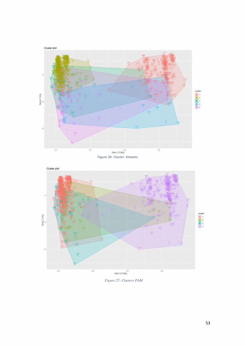
53
Figure 26- Cluster- Kmeans
Figure 27- Clusters PAM

54
As shown above, different methods result in different silhouettes and, consequently, different
cluster numbers, albeit the difference (4 or 5 clusters) is not big.
From this, we may conclude that the database can be naturally grouped into different groups based
on text alone, and that these different groups define clusters that can correlate with other variables
as, possibly, the countries. We may also say that this holds no matter the method adopted. These
clusters represent ITTs awarded by countries part of ESA.
The analysis above was performed considering as the original DTM the dataset.
We performed then some analysis, but the results were not satisfactory. Figure 26 shows the
results using Kmeans. In this method it is necessary to define the cluster's number and according
to the silhouette parameter, the optimal number of clusters is 5.
However, we can easily see that clusters 1 and 2 have significant internal clustering structure,
once the low value indicated by silhouette did not enabled the method to split. In cluster 1,
represented in red, there are clear agglomerations in the right corner. In cluster 2, represented in
green, there is a clear agglomeration in the left corner.
Figure 27 shows the results using PAM. In this method it is also necessary to define the cluster´s
number which optimal value, according to the silhouette parameter, is 4. Inside clusters 1 and 4
we have other clusters that were not separated. In cluster 1, represented in red, there is a clear
agglomeration in the left corner. Cluster 4, represented in purple, presents a clear agglomeration
in the right corner.
Figure 28 - Kmeans - clusters defined inside others clusters

55
Figure 29- PAM- clusters defined inside other clusters
Considering the results were not satisfactory, we proceeded to test a possible dimensionality
reduction, prior to the clustering method. Thus, we used a linear transformation based on Principal
Component Analysis (PCA).
Principal component analysis (PCA) is a multivariate technique that analyzes a data table in which
observations are described by several inter-correlated quantitative dependent variables. Its goal is
to extract the important information from the table, to represent it as a smaller set of new
orthogonal variables called principal components [49].
According to I.T. Jolliffe, “Principal Component Analysis”, the central idea of principal
component analysis (PCA) is to reduce the dimensionality of a data set.” [50]. It is normal that
dataset have many variables that has no relevant information to add. Using PCA, the dataset is
transformed into a new set of variables (note that each variable is a dimension, and when we
reduce dimensions, in fact, we are reducing the number of variables). This smaller dimension new
dataset consists of a new set of variables, the principal components (PCs), which are uncorrelated,
and ordered so that the first few retain most of the variability present in all the original
variables.[49]
The original dataset has 60 dimensions, corresponding to the words previously selected: each
word is equivalent to a dimension, and each document defines a point in a 60-dimensional space.
In this study we considered 10 dimensions, reducing 50 dimensions from the original dataset.
Using “Stats” Package from R, the dataset was converted into a new dataset, with 10 dimensions,
that is, 10 variables. After that, we used kmeans again to look for clusters in this transformed
dataset.
As before, we used the silhouette method to discover the optimal number of clusters.
The optimal number is plotted in Figure 30.

56
The plotted graphic defines as optimal number of 2. However, 2 is clearly too small considering
the dataset size and previous results and so we decided to adopt the second-best peak of the
silhouette analysis. The second-best number of clusters in this case is also number 4, as previously
seen, and this was the number of clusters chosen for the new clustering definition.
Figure 31- Clustering- Kmeans (PCA)
Figure 31 shows the result for clustering method in this study. Comparing with the previous
results shown in figures 26 and 27, it is possible to see that this result is much cleaner, because
there are less overlaps in the projection of the first two principal components, as it was the case
before.
But are there word clusters with a larger fraction of contracts won by certain countries or not? We
thus analyzed inside each cluster the distribution of ITTs per country, in percentage. The result is
shown in table 10.
Figure 30- Optimal cluster numbers- PCA
Table 10 – Distribution of winner countries per cluster

57
Analyzing figure 31 and table 10, it is possible to infer the following important
• Austria, Switzerland, Czech Republic, Estonia, Ireland, Latvia, Norway, Poland,
Romenia, Russia and US have no ITT's awarded in cluster 4. Probably, they do not have
any similarity with ITT's abstract inside this cluster.
• Five countries with more awarded ITTs have similarities in all the defined clusters.
• Germany chance of winning is bigger in cluster 2 than in clusters 1,3 and 4.
• The Netherlands, France, Poland and Portugal have more than 55% awarded ITT in
cluster 2. This fact means that these countries have more chance of winning inside this
cluster than in the others. Another point that we can infer is that these countries has more
efforts and expertise’s in ITTs fields from cluster 2.
• Cluster 2 presents the smallest distance between ITTs, meaning that the similarity
between ITTs abstract is the largest, comparing to the other defined clusters. This fact
can be inferred based on the axis X and Y.
• Cluster 4 has the largest distance between ITTs among the 4 defined clusters. This means
that similarity between ITTs abstract is smaller in comparison with the other defined
clusters. This fact can be inferred based on the axis X and Y.
• Austria, Switzerland and Romenia have the same chance of winning in cluster 2 and 3.
These countries present the same percentage in both clusters.
• Cluster 1 includes the largest number of countries, once 23 of 25 countries belong to this
cluster.
• In cluster 4, Canada and Sweden are the countries with more chance of winning one ESA
ITT.
• All countries have more chance of winning in cluster 2, except Estonia, Latvia, Russia
and USA.
One question that naturally arises is if considering dimensionality reduction using PCA with more
components can produce better results. But which dimension could be better than 10? To answer
to this question, we analyzed how much each component contributes to the total information in
the dataset. In order to do this analysis, the PCA was decomposed into the 60 variables, and it
was possible to evaluate how much each variable contributed with information from the dataset.
Table 11 presents the results.

58
Table 11- Analysis for each component from PCA
eigenvalue variance.percent cumulative.variance
.percent
Dim.1 10.76332351 17.93887252 17.93887
Dim.2 4.30461828 7.17436380 25.11324
Dim.3 1.89764622 3.16274371 28.27598
Dim.4 1.70038101 2.83396834 31.10995
Dim.5 1.67001937 2.78336561 33.89331
Dim.6 1.54713208 2.57855347 36.47187
Dim.7 1.47647905 2.46079842 38.93267
Dim.8 1.36221011 2.27035019 41.20302
Dim.9 1.32317001 2.20528335 43.40830
Dim.10 1.25858318 2.09763864 45.50594
Dim.11 1.23297112 2.05495187 47.56089
Dim.12 1.19529119 1.99215198 49.55304
Dim.13 1.17250587 1.95417645 51.50722
Dim.14 1.14331722 1.90552870 53.41275
Dim.15 1.11834253 1.86390421 55.27665
Dim.16 1.09280663 1.82134439 57.09800
Dim.17 1.07322436 1.78870726 58.88670
Dim.18 1.05572937 1.75954895 60.64625
Dim.19 1.02468802 1.70781336 62.35407
Dim.20 1.00642246 1.67737077 64.03144
Dim.21 0.99426785 1.65711308 65.68855
Dim.22 0.97750863 1.62918106 67.31773
Dim.23 0.94156459 1.56927432 68.88700
Dim.24 0.89975503 1.49959171 70.38660
Dim.25 0.88539126 1.47565210 71.86225
Dim.26 0.88088568 1.46814280 73.33039
Dim.27 0.82863982 1.38106637 74.71146
Dim.28 0.81093151 1.35155251 76.06301
Dim.29 0.80313285 1.33855475 77.40156
Dim.30 0.77584897 1.29308162 78.69465
Dim.31 0.76424285 1.27373808 79.96838
Dim.32 0.74746957 1.24578262 81.21417
Dim.33 0.72887839 1.21479732 82.42896
Dim.34 0.70524131 1.17540219 83.60437
Dim.35 0.68763455 1.14605758 84.75042
Dim.36 0.66319708 1.10532847 85.85575
Dim.37 0.64574260 1.07623766 86.93199
Dim.38 0.63521903 1.05869839 87.99069
Dim.39 0.62213474 1.03689123 89.02758
Dim.40 0.61289827 1.02149711 90.04908
Dim.41 0.57333598 0.95555997 91.00464
Dim.42 0.53447609 0.89079349 91.89543
Dim.43 0.52473915 0.87456526 92.77000
Dim.44 0.51612196 0.86020326 93.63020
Dim.45 0.49582937 0.82638228 94.45658
Dim.46 0.48304328 0.80507213 95.26165
Dim.47 0.45473757 0.75789596 96.01955
Dim.48 0.43935959 0.73226598 96.75182
Dim.49 0.42560514 0.70934190 97.46116
Dim.50 0.34641297 0.57735495 98.03851
Dim.51 0.27038211 0.45063685 98.48915
Dim.52 0.19984780 0.33307967 98.82223
Dim.53 0.17492656 0.29154427 99.11377
Dim.54 0.15264156 0.25440259 99.36818
Dim.55 0.13763539 0.22939232 99.59757
Dim.56 0.08320977 0.13868294 99.73625
Dim.57 0.05263110 0.08771849 99.82397
Dim.58 0.05034491 0.08390818 99.90788
Dim.59 0.03313844 0.05523073 99.96311
Dim.60 0.02213507 0.03689179 100.00000

59
Analyzing the cumulative variance, it is possible to conclude that 24 dimensions explain more
than 70% of the dataset information. Our main goal is to verify if using a larger dimension
produces better results for relating cluster of words to the chance of winning. We kept the same
number of clusters from the first PCA plot result, k=4, and we used the same cluster validation
method as before, the silhouette. The clusters found are shown in figure 32.
The clusters plot is very similar to the clusters with 10 dimensions, but the countries distribution
changed, as shown in table 12.
Table 12- Countries distribution -PCA with 24 dimensions
From these results, it is possible to conclude that:
- With more dimensions the countries percentage changed.
- All the countries present more ITTs in cluster 2.
- Cluster 4 almost “disappeared”.
After these two exploratory analyses, the result was not completely satisfactory. Changing the
PCA dimensions did not make possible to verify if there were cluster of words related to a chance
of winning from one certain country. Probably, using different clusters parameters, as the number
of clusters and validation parameter, or non-linear dimensionality reduction methods that could
enable the adoption of a larger set of words, we could improve on the clustering results. It was
conclusive, however, that the ESA ITT are agglomerated in clusters of words.
Other questions remain to be answered for a complete understanding of how cluster of words in
ESA ITT define a chance of a country winning an ITT award. It is necessary to use different
methods from those used in this study, and investigate cluster characteristics, as: How words are
related with each other so that they form coherent ideas and concepts behind the ITTs?
Figure 32- kmeans with 24 dimensions

60
CONCLUSION
From this study one conclusion can clearly be made: there are relations between ITT abstract
words and a chance of certain country winning an ESA ITT.
The study started with the analysis of the relationship between countries that were awarded ESA
ITTs, with ESA Offices and ESA Programs. From simple graphical analysis of matrices and
correlations, and from further analysis of these results we saw that it seems to exist a relationship
between number of employees dedicated to space sector, the countries organization to bid in ESA
and the success in these bids. We also discovered a strong anti-correlation between the major
European space player countries in ESA programs.
Then we employed text mining techniques to build document term matrices, the central data
structure of this thesis. We developed a large set of R codes based on reference packages as TM,
to perform the analysis. We developed logistic regression and stepwise models for each one of
the 5 countries: Belgium, France, Great Britain (UK), Germany and Italy.
Simple logistic regression has more degrees of freedom than stepwise models, probably because
of multicollinearity, thus it was natural to see that stepwise methods had better results than logistic
regression. We selected the best models for each one of the 5 countries.
After that, we studied the prediction from these models, comparing the predicted value and what
really happened. Using different methods, we concluded that, for more than 50% of the ITTs, the
prediction works better than random. Also, the model prediction is 100% right, when the predicted
value is bigger than 80%.
Considering the area under ROC the constructed models indicate that the probability of winning
is higher than 50%. This means that the regression models are not random and in fact, certain
words in ITTs abstracts have relation with the chance of certain country award an ITT. Cut-off
points were defined for each country, showing the chance that a certain country must win an ITT
without any model. The largest point was from Germany.
When some specific words appear in an ITT that can raise the chance of winning. This was
explored trough the ODDs ratio analysis of the model variables in each of the 5 more awarded
countries.
Then, we performed an exploratory analysis of how ITT abstracts clustered in the space defined
by selected words, trying to find relationships between clusters and winning countries. Before any
clustering, a correlation matrix was constructed, and a clustering tendency among the documents
was detected. Then clusters were constructed using different hierarchical and non-hierarchical
methods, all of them showing that the documents can be organized in clusters, although we could
not find a correlation between the clusters and the ITT awarded country. This problem leaves the
door open for further studies.
In the future, other questions should be answered for a better understanding of how words in ESA
ITT abstract can predict what country will win an ITT, namely,
• How words relate to each other to form concepts within clusters?
• What ITTs can be considered "defining" for those clusters, if any?
• How those agglomerations can be associated to the countries winning each ITT?
These questions open new study possibilities as, for example, unexplored clustering methods,
non-linear dimensionality reduction methods, text manipulation techniques and cluster validation.

61
REFERENCES
[1] https://www.rdocumentation.org/packages/XLConnect/versions/0.2-15. [Accessed: April 4,
2019]
[2] R “Help” tool [3] “Regular expression - Wikipedia, the free encyclopedia”, March 10, 2019. [Online].
Available: http://en.wikipedia.org/wiki/Regular_expression. [Accessed: March 31, 2019].
[4] Hogg et al., “Probability and Statistical Inference”, Pearson, Ninth edition, ISBN 978-0-321-
92327-1, page 105
[5] W. L. Hays, Statistics, 5th ed., New York: Holt, Rinehart and Winston, 1994.
[6] Hogg et al., “Probability and Statistical Inference”, Pearson, Ninth edition, ISBN 978-0-321-
92327-1, page 192.
[7][10]”Mandatory
programs”[Online].Available:http://www.rosa.ro/index.php/en/esa/programe-obligatorii/83-esa-
cat/romania-membru-esa [Accessed: March 31,2019].
[8]”Doing business with ESA” [Online].Available: https://www.spacecenter.ch/activities/businesswithesa/ [Accessed: March 31, 2019].
[9]”Strategic Baseline Portugal Space 2030” [Online].Available:
https://www.ptspace.pt/strategic-baseline/[Acessed: March 31, 2019].
[11] “International and European Institutions in Brussels” [Online]. Available: (https://be.brussels/links-en/brussels-regional-and-international-institutions-in-brussels/international-and-european-institutions-in-brussels?set_language=en) [Accessed in April 03, 2019]. [12] “Welcome to ESA” [Online]. Available:
https://www.esa.int/About_Us/Welcome_to_ESA/Brussels_Office [Accessed in April 03,
2019]
[13] “Earth Observation Satellites”[Online]. Available: http://www.asc-
csa.gc.ca/eng/satellites/default-eo.asp [Accessed in April 03, 2019].
[14] “Space Lands in Spain” [Online]. Available: https://www.esa.int/Education/Space_lands_in_Spanish_classrooms_with_ESERO_Spain
[Accessed in April 03, 2019].
[15]” Space Research” [Online]. Available: https://www.dlr.de/dlr/en/desktopdefault.aspx/tabid-
10196/342_read-265/#/gallery/283 [Accessed in April 4, 2019].
[16] "Institutes” [Online]. Available:https://www.dlr.de/dlr/en/desktopdefault.aspx/tabid-10211/
[Accessed in April 4, 2019].
[17] “https://www.asi.it/en/agency” [Online]. [Accessed in April 4, 2019]
[18]
https://www.esa.int/About_Us/Business_with_ESA/How_to_do/Industrial_policy_and_geograp
hical_distribution [Online]. [Accessed in April 4, 2019]
[19] https://www.ruag.com/en/about-ruag/organisation/divisions/ruag-space [Online]. Accessed April 21, 2019] [20] https://cnes.fr/en [Online].[ Accessed in April 4, 2019]
[21] https://www.gov.uk/government/organisations/uk-space-agency [Online]. [Accessed in
April 4, 2019]
[22] Ronen Feldman &James Sanger: The Text Mining Handbook: Advanced Approaches in
Analyzing Unstructured Data - Cambridge University Press, 2007
[23] Tandel et al., “A Survey on Text Mining Techniques”.5th International Conference on
Advanced Computing & Communication Systems (ICACCS 2019)
[24]K. Welbers et al.,“ Text Analysis in R”

62
https://doi.org/10.1080/19312458.2017.1387238
[25] Julia Silge & David Robinson. “Text Mining with R” June 2017- First Edition- O´Reilly.
Page 2.
[26] Ingo Feinerer, July 29, 2018,” Introduction to TM Package text mining in R” -– “ R Help directory”. [27] Shen, D., and Lu, Z. (2006). Computation of correlation coefficient and its confidence
interval in SAS (r). SUGI 31 (March 26-29, 2006), paper 170-31. Available online at
http://www2.sas.com/proceedings/sugi31/170-31.pdf.
[28] R. Hogg et al., “Probability and Statistical Inference”, Pearson, Ninth edition, ISBN 978-0-
321-92327-1, page 354.
[29] A.Bager et al.,(2017)” Addressing multicollinearity in regression models: a ridge regression
application”. Online at: https://mpra.ub.uni-muenchen.de/81390/3/MPRA_paper_81357.pdf
[Accessed in April 6, 2019]
[30] Peter Bruce & Andrew Bruce, (2017) in “Practical Statistics for Data Scientists”, page 262
[31]J.Gareth et al.,2013 “An Introduction to Statistical Learning with Applications in R”, Springler, 2013. Pages 209 to 212
[32] T.Hastie et al.,“ The elements of Statistical Learning – Data Mining, Inference and
Prediction”, Springler- Second Edition- page 60.
[33] G. Shmueli,” To Explain or to Predict?” -Statistical Science 2010, Vol. 25, No. 3, 289–310
DOI: 10.1214/10-STS330 © Institute of Mathematical Statistics, 2010
[34] Park, Hyeoun-Ae, J Korean Acad Nurs Vol.43 No.2 April 2013,
http://dx.doi.org/10.4040/jkan.2013.43.2.154
[35] T. Alpuim, Modelos Lineares, Chapter 5. Notes for the course Linear Models - Faculty of
Science of the University of Lisbon.
[36]” Confusion Matrix”[Online]. Available: https://www.ic.unicamp.br/~wainer/cursos/1s2012/mc906/Confusion.pdf [Accessed April 7,
2019]
[37] “On determining the most appropriate test cut-off value: the case of tests with continuous
results”, Published online 2016 Oct 15. doi: 10.11613/BM.2016.034
[38] T.Fawcett, “An introduction to ROC Analysis”. T. Fawcett / Pattern Recognition Letters 27 (2006) 861–874. Available online 19 December 2005
[39] Tandel et al.,” A Survey on Text Mining Techniques, 2019 5th International Conference on
Advanced Computing & Communication Systems.
[40] Lior Rokach &Oded Maimon, “Clustering Methods- Chapter 15”. [Online] Available: https://www.cs.swarthmore.edu/~meeden/cs63/s16/reading/Clustering.pdf [Accessed May
11,2019]
[41] Peter J. Rousseeuw (1987). "Silhouettes: A Graphical Aid to the Interpretation and
Validation of Cluster Analysis". Computational and Applied Mathematics. 20: 53–65.
doi:10.1016/0377-0427(87)90125-7.
[42] http://sfb649.wiwi.hu-berlin.de/fedc_homepage/xplore/tutorials/xaghtmlnode54.html
[Online]. Accessed: 04/05/2019
[43] https://www.datanovia.com/en/courses/partitional-clustering-in-r-the-essentials/ [Online].
Accessed: 05/05/2019
[44] Oded Maimon & Lior Rokach, “Data Mining and Knowledge Discovery Handbook”, Second
Edition, Springer, 2010, DOI 10.1007/978-0-387-09823-4, page 934-935
[45] Alboukadel Kassambara, “Practical Guide to Cluster Analysis in R- Unsupervised Machine
Learning”, STHDA, Edition 1. Pag 34
[46] https://uc-r.github.io/hc_clustering [Online]. Accessed [May 12, 2019]

63
[47]G. Brook et at.,” clValid: An R Package for Cluster Validation”, Journal of Statistical Software, March 2008, Volume 25, Issue 4.
[48] Peter J. Rousseeuw (1987). "Silhouettes: A Graphical Aid to the Interpretation and
Validation of Cluster Analysis". Computational and Applied Mathematics. 20: 53–65.
doi:10.1016/0377-0427(87)90125-7.
[49] John Wiley& Sons,Inc. WIREs CompStat 2010 2433–459 [Online]. Available :
https://www.utdallas.edu/~herve/abdi-awPCA2010.pdf [Accessed in May 18 2019]
[50] I.T. Jolliffe, “Principal Component Analysis”, Second Edition, Springer, 2002, New York

64
ANNEX
DEVELOPED MODEL FOR ALL COUNTRIES (“R RESULTS”)
Germany – Developed Models and Area Under ROC curve
> summary(model_logistic_DE) # summary of logistic model for Germany Call: glm(formula = resVec_DE ~ ., family = binomial, data = m_t1) Deviance Residuals: Min 1Q Median 3Q Max -1.5303 -0.6859 -0.5369 -0.2977 2.4408 Coefficients: Estimate Std. Error z value Pr(>|z|) (Intercept) -1.6083026 0.1995781 -8.059 7.72e-16 *** aim 0.0895983 0.1467891 0.610 0.54161 applic -0.1013428 0.1375350 -0.737 0.46121 capabl 0.1237862 0.1623258 0.763 0.44571 differ 0.1019318 0.1240789 0.822 0.41136 follow 0.2711489 0.1766084 1.535 0.12471 ground 0.2811396 0.1116534 2.518 0.01180 * identifi 0.2481045 0.1621780 1.530 0.12606 integr 0.0675429 0.1290603 0.523 0.60074 part 0.1118275 0.1396563 0.801 0.42329 potenti -0.2127593 0.1802934 -1.180 0.23797 propos -0.2060894 0.1610986 -1.279 0.20080 specif -0.2421509 0.1442248 -1.679 0.09316 . time -0.0463693 0.1845933 -0.251 0.80166 allow 0.0664308 0.1681415 0.395 0.69278 assess 0.0420730 0.1500536 0.280 0.77918 contractor -0.0503053 0.1748446 -0.288 0.77357 european -0.0450776 0.1331298 -0.339 0.73491 exist 0.0683644 0.1914850 0.357 0.72108 increas -0.0456826 0.1964837 -0.233 0.81615 limit -0.7643950 0.3003704 -2.545 0.01093 * order 0.4022834 0.1692663 2.377 0.01747 * power -0.0169763 0.1029899 -0.165 0.86907 product 0.1595505 0.0992838 1.607 0.10805 result 0.1524122 0.1990737 0.766 0.44391 techniqu 0.0384960 0.1428249 0.270 0.78752 earth -0.1198963 0.1359471 -0.882 0.37781 futur -0.3510899 0.1773523 -1.980 0.04775 * well -0.1486133 0.1959347 -0.758 0.44816 within 0.2261312 0.2051738 1.102 0.27040 avail 0.1827054 0.1874631 0.975 0.32975 entiti 0.7108163 0.3492520 2.035 0.04183 * generat -0.4235633 0.2358631 -1.796 0.07253 . improv -0.1038298 0.1722144 -0.603 0.54657 one 0.0017409 0.1954456 0.009 0.99289 programm 0.1463704 0.2579264 0.567 0.57038 activiti 0.2057346 0.4985816 0.413 0.67987 activity -0.2859238 0.2839058 -1.007 0.31388 concept 0.3177697 0.1108815 2.866 0.00416 ** emits -0.0009751 0.3606952 -0.003 0.99784 full 0.4724942 0.2201307 2.146 0.03184 * incl 1.1560522 0.7530430 1.535 0.12474

65
industrial -0.6480449 1.6205696 -0.400 0.68924 news -2.0276921 1.1653881 -1.740 0.08187 . nonprimes 1.5636916 1.3810854 1.132 0.25754 pleas 0.0910301 0.3875052 0.235 0.81428 polici -0.3659634 0.6739601 -0.543 0.58713 policy 0.2014990 0.9784931 0.206 0.83685 restrict 0.1141667 0.4717337 0.242 0.80877 nonprim -0.8744894 0.8756684 -0.999 0.31796 term 0.2319096 0.1880167 1.233 0.21741 demonstr 0.0048615 0.1496350 0.032 0.97408 manufactur -0.0251217 0.1224696 -0.205 0.83747 main -0.2035419 0.2020711 -1.007 0.31380 particular -0.1674443 0.2303660 -0.727 0.46731 spacecraft -0.0910711 0.1273899 -0.715 0.47467 possibl -0.2401661 0.1822895 -1.317 0.18767 select -0.0799168 0.1859587 -0.430 0.66737 two -0.1267851 0.1920082 -0.660 0.50905 analysi -0.0447932 0.1575852 -0.284 0.77622 valid 0.0718330 0.1348328 0.533 0.59420 --- Signif. codes: 0 ‘***’ 0.001 ‘**’ 0.01 ‘*’ 0.05 ‘.’ 0.1 ‘ ’ 1 (Dispersion parameter for binomial family taken to be 1) Null deviance: 759.27 on 756 degrees of freedom Residual deviance: 682.88 on 696 degrees of freedom AIC: 804.88 Number of Fisher Scoring iterations: 5
> summary(mstep_DE) # summary of stepwise forward model for Germany Call: glm(formula = resVec_DE ~ concept + limit + order + futur + ground + full + product + generat, family = binomial, data = m_t1) Deviance Residuals: Min 1Q Median 3Q Max -1.6327 -0.6825 -0.6180 -0.3853 2.1871 Coefficients: Estimate Std. Error z value Pr(>|z|) (Intercept) -1.55850 0.13373 -11.654 < 2e-16 *** concept 0.29128 0.09564 3.046 0.00232 ** limit -0.73729 0.26724 -2.759 0.00580 ** order 0.33995 0.13300 2.556 0.01059 * futur -0.32878 0.15429 -2.131 0.03309 * ground 0.22004 0.09746 2.258 0.02395 * full 0.38207 0.17421 2.193 0.02829 * product 0.16883 0.08160 2.069 0.03855 * generat -0.27864 0.20318 -1.371 0.17026 --- Signif. codes: 0 ‘***’ 0.001 ‘**’ 0.01 ‘*’ 0.05 ‘.’ 0.1 ‘ ’ 1 (Dispersion parameter for binomial family taken to be 1) Null deviance: 759.27 on 756 degrees of freedom Residual deviance: 715.80 on 748 degrees of freedom AIC: 733.8

66
Number of Fisher Scoring iterations: 5
> summary(mstepb_DE) # summary of stepwise both model for Germany Call: glm(formula = resVec_DE ~ concept + limit + order + futur + ground + full + product + generat, family = binomial, data = m_t1) Deviance Residuals: Min 1Q Median 3Q Max -1.6327 -0.6825 -0.6180 -0.3853 2.1871 Coefficients: Estimate Std. Error z value Pr(>|z|) (Intercept) -1.55850 0.13373 -11.654 < 2e-16 *** concept 0.29128 0.09564 3.046 0.00232 ** limit -0.73729 0.26724 -2.759 0.00580 ** order 0.33995 0.13300 2.556 0.01059 * futur -0.32878 0.15429 -2.131 0.03309 * ground 0.22004 0.09746 2.258 0.02395 * full 0.38207 0.17421 2.193 0.02829 * product 0.16883 0.08160 2.069 0.03855 * generat -0.27864 0.20318 -1.371 0.17026 --- Signif. codes: 0 ‘***’ 0.001 ‘**’ 0.01 ‘*’ 0.05 ‘.’ 0.1 ‘ ’ 1 (Dispersion parameter for binomial family taken to be 1) Null deviance: 759.27 on 756 degrees of freedom Residual deviance: 715.80 on 748 degrees of freedom AIC: 733.8 Number of Fisher Scoring iterations: 5
> AIC(mstep_DE,mstepb_DE,mstepbw_DE)# shows AIC number from all stepwise models developed for Germany df AIC mstep_DE 9 733.8035 mstepb_DE 9 733.8035 mstepbw_DE 12 732.1902
Area under roc curve > (area_DE <- performance(pred_DE, "auc")) An object of class "performance" Slot "x.name": [1] "None" Slot "y.name": [1] "Area under the ROC curve" Slot "alpha.name": [1] "none" Slot "x.values": list() Slot "y.values": [[1]]

67
[1] 0.656492 Slot "alpha.values": list()
Belgium – Developed Models and Area under ROC curve
> summary(model_logistic_BE) # summary of logistic model for Belgium Call: glm(formula = resVec_BE ~ ., family = binomial, data = m_t1) Deviance Residuals: Min 1Q Median 3Q Max -1.2849 -0.4914 -0.3638 -0.2129 2.5279 Coefficients: Estimate Std. Error z value Pr(>|z|) (Intercept) -2.071336 0.261214 -7.930 2.2e-15 *** aim 0.336544 0.187159 1.798 0.0722 . applic -0.020679 0.192770 -0.107 0.9146 capabl 0.306545 0.209590 1.463 0.1436 differ 0.181107 0.167951 1.078 0.2809 follow 0.003997 0.264130 0.015 0.9879 ground -0.242294 0.194510 -1.246 0.2129 identifi -0.161657 0.264791 -0.611 0.5415 integr 0.196683 0.159549 1.233 0.2177 part -0.006673 0.205576 -0.032 0.9741 potenti 0.095254 0.238320 0.400 0.6894 propos -0.181411 0.274080 -0.662 0.5080 specif 0.136998 0.206509 0.663 0.5071 time -0.084787 0.297224 -0.285 0.7754 allow 0.055970 0.267313 0.209 0.8342 assess -0.456231 0.302885 -1.506 0.1320 contractor 0.283906 0.164073 1.730 0.0836 . european 0.142759 0.162592 0.878 0.3799 exist -0.124214 0.301210 -0.412 0.6801 increas 0.066401 0.280338 0.237 0.8128 limit -0.424241 0.441994 -0.960 0.3371 order -0.122711 0.271130 -0.453 0.6508 power -0.133637 0.170826 -0.782 0.4340 product 0.091601 0.135369 0.677 0.4986 result -0.390632 0.372219 -1.049 0.2940 techniqu 0.113674 0.199383 0.570 0.5686 earth 0.065338 0.175995 0.371 0.7105 futur 0.036794 0.205358 0.179 0.8578 well 0.125882 0.267978 0.470 0.6385 within -0.297386 0.324753 -0.916 0.3598 avail -0.165837 0.337799 -0.491 0.6235 entiti -0.648820 0.688718 -0.942 0.3462 generat -0.393946 0.344634 -1.143 0.2530 improv -0.576049 0.314618 -1.831 0.0671 . one 0.118880 0.286049 0.416 0.6777 programm 0.194503 0.300247 0.648 0.5171 activiti 0.677451 0.648917 1.044 0.2965 activity 0.286859 0.347162 0.826 0.4086 concept -0.155584 0.244040 -0.638 0.5238 emits 0.522745 0.533520 0.980 0.3272 full -0.065384 0.346282 -0.189 0.8502

68
incl -13.790198 684.686935 -0.020 0.9839 industrial 0.640004 1.698279 0.377 0.7063 news -2.199005 1.484948 -1.481 0.1386 nonprimes 0.173259 1.762160 0.098 0.9217 pleas 0.256990 0.519608 0.495 0.6209 polici 1.077036 0.611192 1.762 0.0780 . policy 0.083285 1.494623 0.056 0.9556 restrict -0.653939 0.791581 -0.826 0.4087 nonprim 12.956272 684.687061 0.019 0.9849 term -0.321365 0.364230 -0.882 0.3776 demonstr 0.232603 0.194464 1.196 0.2316 manufactur 0.035931 0.190367 0.189 0.8503 main -0.207637 0.298727 -0.695 0.4870 particular 0.010145 0.326385 0.031 0.9752 spacecraft -0.002068 0.200292 -0.010 0.9918 possibl 0.013928 0.267414 0.052 0.9585 select -0.260903 0.287239 -0.908 0.3637 two 0.414372 0.240093 1.726 0.0844 . analysi -0.466930 0.311736 -1.498 0.1342 valid -0.123570 0.220685 -0.560 0.5755 --- Signif. codes: 0 ‘***’ 0.001 ‘**’ 0.01 ‘*’ 0.05 ‘.’ 0.1 ‘ ’ 1 (Dispersion parameter for binomial family taken to be 1) Null deviance: 471.19 on 756 degrees of freedom Residual deviance: 419.40 on 696 degrees of freedom AIC: 541.4 Number of Fisher Scoring iterations: 15
> summary(mstep_BE) # summary of stepwise forward model for Belgium Call: glm(formula = resVec_BE ~ limit + assess + aim + generat + capabl + improv + analysi + contractor + incl + polici, family = binomial, data = m_t1) Deviance Residuals: Min 1Q Median 3Q Max -1.2016 -0.4869 -0.4075 -0.2919 2.5807 Coefficients: Estimate Std. Error z value Pr(>|z|) (Intercept) -2.0726 0.1897 -10.928 <2e-16 *** limit -0.6203 0.4064 -1.526 0.1269 assess -0.4415 0.2796 -1.579 0.1144 aim 0.2928 0.1568 1.868 0.0618 . generat -0.3740 0.3090 -1.210 0.2261 capabl 0.3356 0.1802 1.862 0.0626 . improv -0.4234 0.2831 -1.495 0.1348 analysi -0.4521 0.2840 -1.592 0.1114 contractor 0.2848 0.1377 2.068 0.0386 * incl -1.1482 0.4843 -2.371 0.0178 * polici 0.6149 0.3826 1.607 0.1080 --- Signif. codes: 0 ‘***’ 0.001 ‘**’ 0.01 ‘*’ 0.05 ‘.’ 0.1 ‘ ’ 1 (Dispersion parameter for binomial family taken to be 1)

69
Null deviance: 471.19 on 756 degrees of freedom Residual deviance: 442.52 on 746 degrees of freedom AIC: 464.52 Number of Fisher Scoring iterations: 6
> summary(mstepb_BE) # summary of stepwise both model for Belgium Call: glm(formula = resVec_BE ~ limit + assess + aim + capabl + improv + analysi + contractor + incl + polici, family = binomial, data = m_t1) Deviance Residuals: Min 1Q Median 3Q Max -1.2165 -0.4795 -0.4256 -0.2937 2.5566 Coefficients: Estimate Std. Error z value Pr(>|z|) (Intercept) -2.1049 0.1875 -11.225 <2e-16 *** limit -0.6655 0.4059 -1.639 0.1011 assess -0.4145 0.2755 -1.504 0.1325 aim 0.2444 0.1507 1.622 0.1047 capabl 0.3277 0.1736 1.888 0.0591 . improv -0.4269 0.2813 -1.518 0.1291 analysi -0.5085 0.2808 -1.811 0.0701 . contractor 0.2961 0.1378 2.149 0.0316 * incl -1.1806 0.4859 -2.430 0.0151 * polici 0.6335 0.3834 1.652 0.0985 . --- Signif. codes: 0 ‘***’ 0.001 ‘**’ 0.01 ‘*’ 0.05 ‘.’ 0.1 ‘ ’ 1 (Dispersion parameter for binomial family taken to be 1) Null deviance: 471.19 on 756 degrees of freedom Residual deviance: 444.28 on 747 degrees of freedom AIC: 464.28 Number of Fisher Scoring iterations: 6 > summary(mstepbw_BE)# summary of stepwise backward model for Belgium Call: glm(formula = resVec_BE ~ aim + capabl + assess + contractor + limit + improv + incl + polici + analysi, family = binomial, data = m_t1) Deviance Residuals: Min 1Q Median 3Q Max -1.2165 -0.4795 -0.4256 -0.2937 2.5566 Coefficients: Estimate Std. Error z value Pr(>|z|) (Intercept) -2.1049 0.1875 -11.225 <2e-16 *** aim 0.2444 0.1507 1.622 0.1047 capabl 0.3277 0.1736 1.888 0.0591 . assess -0.4145 0.2755 -1.504 0.1325 contractor 0.2961 0.1378 2.149 0.0316 *

70
limit -0.6655 0.4059 -1.639 0.1011 improv -0.4269 0.2813 -1.518 0.1291 incl -1.1806 0.4859 -2.430 0.0151 * polici 0.6335 0.3834 1.652 0.0985 . analysi -0.5085 0.2808 -1.811 0.0701 . --- Signif. codes: 0 ‘***’ 0.001 ‘**’ 0.01 ‘*’ 0.05 ‘.’ 0.1 ‘ ’ 1 (Dispersion parameter for binomial family taken to be 1) Null deviance: 471.19 on 756 degrees of freedom Residual deviance: 444.28 on 747 degrees of freedom AIC: 464.28 Number of Fisher Scoring iterations: 6
> AIC(mstep_BE,mstepb_BE,mstepbw_BE)# shows AIC number from all stepwise models developed for Belgium df AIC mstep_BE 11 464.5180 mstepb_BE 10 464.2837 mstepbw_BE 10 464.2837
Area under ROC curve > (area_BE <- performance(pred_BE, "auc")) An object of class "performance" Slot "x.name": [1] "None" Slot "y.name": [1] "Area under the ROC curve" Slot "alpha.name": [1] "none" Slot "x.values": list() Slot "y.values": [[1]] [1] 0.6729561 Slot "alpha.values": list()
Italy- Developed models and Area under ROC curve > summary(model_logistic_IT) # summary of logistic model for Italy Call: glm(formula = resVec_IT ~ ., family = binomial, data = m_t1) Deviance Residuals: Min 1Q Median 3Q Max -1.4036 -0.5741 -0.4203 -0.2059 2.7874 Coefficients: Estimate Std. Error z value Pr(>|z|) (Intercept) -1.58413 0.21813 -7.262 3.8e-13 ***

71
aim 0.10094 0.17842 0.566 0.57158 applic -0.15576 0.18506 -0.842 0.39996 capabl 0.25729 0.18089 1.422 0.15492 differ 0.01053 0.14504 0.073 0.94213 follow -0.38349 0.27122 -1.414 0.15738 ground 0.18918 0.12847 1.473 0.14086 identifi -0.18149 0.20352 -0.892 0.37253 integr -0.47972 0.22760 -2.108 0.03506 * part -0.35514 0.25780 -1.378 0.16833 potenti 0.06966 0.19774 0.352 0.72463 propos 0.14735 0.17471 0.843 0.39898 specif -0.08324 0.20004 -0.416 0.67732 time -0.04358 0.22798 -0.191 0.84839 allow 0.17440 0.18469 0.944 0.34503 assess -0.49817 0.23692 -2.103 0.03549 * contractor -0.14690 0.27948 -0.526 0.59914 european 0.48600 0.15459 3.144 0.00167 ** exist -0.26186 0.24502 -1.069 0.28520 increas -0.08213 0.23701 -0.347 0.72895 limit -0.07134 0.26110 -0.273 0.78466 order 0.19315 0.20634 0.936 0.34925 power 0.09304 0.09892 0.941 0.34695 product -0.13303 0.13412 -0.992 0.32127 result 0.24337 0.23367 1.041 0.29765 techniqu 0.32094 0.12580 2.551 0.01073 * earth 0.36625 0.13473 2.718 0.00656 ** futur 0.17536 0.16885 1.039 0.29903 well -0.50356 0.24781 -2.032 0.04215 * within -0.15449 0.25371 -0.609 0.54257 avail 0.02127 0.24523 0.087 0.93090 entiti 0.15252 0.48692 0.313 0.75410 generat 0.02090 0.21817 0.096 0.92368 improv -0.04536 0.17830 -0.254 0.79917 one -0.33293 0.25907 -1.285 0.19876 programm -0.73611 0.45854 -1.605 0.10842 activiti -0.04755 0.66535 -0.071 0.94302 activity -0.53787 0.36505 -1.473 0.14064 concept -0.06447 0.16280 -0.396 0.69211 emits 2.14487 1.18721 1.807 0.07082 . full 0.01922 0.26912 0.071 0.94307 incl -0.80441 1.26698 -0.635 0.52549 industrial -12.86060 622.69720 -0.021 0.98352 news -1.01846 1.53227 -0.665 0.50626 nonprimes 14.58764 622.69921 0.023 0.98131 pleas -0.18176 0.49177 -0.370 0.71168 polici -1.10533 1.41952 -0.779 0.43618 policy -1.98866 0.92864 -2.141 0.03223 * restrict 0.25988 0.58037 0.448 0.65430 nonprim 0.76130 1.43912 0.529 0.59680 term 0.40039 0.19694 2.033 0.04205 * demonstr -0.14066 0.18358 -0.766 0.44354 manufactur -0.50670 0.27296 -1.856 0.06341 . main 0.45382 0.20971 2.164 0.03046 * particular -0.12663 0.29012 -0.436 0.66250 spacecraft -0.05929 0.14817 -0.400 0.68903 possibl 0.25482 0.18853 1.352 0.17650 select -0.11661 0.22916 -0.509 0.61086 two 0.10406 0.21783 0.478 0.63285 analysi 0.17148 0.16640 1.031 0.30277 valid -0.14931 0.18057 -0.827 0.40831

72
--- Signif. codes: 0 ‘***’ 0.001 ‘**’ 0.01 ‘*’ 0.05 ‘.’ 0.1 ‘ ’ 1 (Dispersion parameter for binomial family taken to be 1) Null deviance: 634.58 on 756 degrees of freedom Residual deviance: 525.85 on 696 degrees of freedom AIC: 647.85 Number of Fisher Scoring iterations: 15
> summary(mstep_IT)# summary of stepwise forward model for Italy Call: glm(formula = resVec_IT ~ policy + emits + european + integr + manufactur + techniqu + earth + part + main + assess + term + well + allow + activity + programm + follow, family = binomial, data = m_t1) Deviance Residuals: Min 1Q Median 3Q Max -1.3998 -0.6040 -0.4502 -0.2502 2.9770 Coefficients: Estimate Std. Error z value Pr(>|z|) (Intercept) -1.6089 0.1698 -9.478 < 2e-16 *** policy -2.0035 0.6326 -3.167 0.00154 ** emits 1.6877 0.5800 2.910 0.00361 ** european 0.4217 0.1336 3.157 0.00159 ** integr -0.4242 0.2241 -1.893 0.05841 . manufactur -0.5517 0.2709 -2.037 0.04168 * techniqu 0.2929 0.1150 2.548 0.01084 * earth 0.3197 0.1109 2.883 0.00394 ** part -0.3314 0.2233 -1.484 0.13771 main 0.4647 0.1901 2.444 0.01451 * assess -0.3551 0.2016 -1.761 0.07826 . term 0.4474 0.1739 2.573 0.01009 * well -0.4934 0.2292 -2.153 0.03133 * allow 0.2792 0.1563 1.786 0.07408 . activity -0.5489 0.3096 -1.773 0.07623 . programm -0.6062 0.3827 -1.584 0.11317 follow -0.3276 0.2291 -1.430 0.15284 --- Signif. codes: 0 ‘***’ 0.001 ‘**’ 0.01 ‘*’ 0.05 ‘.’ 0.1 ‘ ’ 1 (Dispersion parameter for binomial family taken to be 1) Null deviance: 634.58 on 756 degrees of freedom Residual deviance: 550.32 on 740 degrees of freedom AIC: 584.32 Number of Fisher Scoring iterations: 6
> summary(mstepb_IT)# summary of stepwise both model for Italy Call: glm(formula = resVec_IT ~ policy + emits + european + integr + manufactur + techniqu + earth + part + main + assess + term + well + allow + activity + programm + follow, family = binomial, data = m_t1)

73
Deviance Residuals: Min 1Q Median 3Q Max -1.3998 -0.6040 -0.4502 -0.2502 2.9770 Coefficients: Estimate Std. Error z value Pr(>|z|) (Intercept) -1.6089 0.1698 -9.478 < 2e-16 *** policy -2.0035 0.6326 -3.167 0.00154 ** emits 1.6877 0.5800 2.910 0.00361 ** european 0.4217 0.1336 3.157 0.00159 ** integr -0.4242 0.2241 -1.893 0.05841 . manufactur -0.5517 0.2709 -2.037 0.04168 * techniqu 0.2929 0.1150 2.548 0.01084 * earth 0.3197 0.1109 2.883 0.00394 ** part -0.3314 0.2233 -1.484 0.13771 main 0.4647 0.1901 2.444 0.01451 * assess -0.3551 0.2016 -1.761 0.07826 . term 0.4474 0.1739 2.573 0.01009 * well -0.4934 0.2292 -2.153 0.03133 * allow 0.2792 0.1563 1.786 0.07408 . activity -0.5489 0.3096 -1.773 0.07623 . programm -0.6062 0.3827 -1.584 0.11317 follow -0.3276 0.2291 -1.430 0.15284 --- Signif. codes: 0 ‘***’ 0.001 ‘**’ 0.01 ‘*’ 0.05 ‘.’ 0.1 ‘ ’ 1 (Dispersion parameter for binomial family taken to be 1) Null deviance: 634.58 on 756 degrees of freedom Residual deviance: 550.32 on 740 degrees of freedom AIC: 584.32 Number of Fisher Scoring iterations: 6
> summary(mstepbw_IT)# summary of stepwise backward model for Italy Call: glm(formula = resVec_IT ~ follow + ground + integr + part + assess + european + techniqu + earth + well + programm + activity + emits + policy + term + manufactur + main, family = binomial, data = m_t1) Deviance Residuals: Min 1Q Median 3Q Max -1.4596 -0.6038 -0.4430 -0.2500 3.0044 Coefficients: Estimate Std. Error z value Pr(>|z|) (Intercept) -1.5924 0.1683 -9.462 < 2e-16 *** follow -0.3610 0.2313 -1.561 0.11853 ground 0.1718 0.1115 1.540 0.12344 integr -0.4400 0.2223 -1.979 0.04780 * part -0.3480 0.2220 -1.568 0.11699 assess -0.3782 0.2059 -1.836 0.06631 . european 0.4177 0.1370 3.049 0.00230 ** techniqu 0.3165 0.1140 2.777 0.00548 ** earth 0.2985 0.1104 2.703 0.00688 ** well -0.5148 0.2286 -2.252 0.02430 * programm -0.5951 0.3771 -1.578 0.11453

74
activity -0.5368 0.3099 -1.732 0.08320 . emits 1.6521 0.5372 3.075 0.00210 ** policy -1.9068 0.5999 -3.178 0.00148 ** term 0.4586 0.1735 2.644 0.00820 ** manufactur -0.5472 0.2725 -2.008 0.04467 * main 0.4773 0.1883 2.534 0.01127 * --- Signif. codes: 0 ‘***’ 0.001 ‘**’ 0.01 ‘*’ 0.05 ‘.’ 0.1 ‘ ’ 1 (Dispersion parameter for binomial family taken to be 1) Null deviance: 634.58 on 756 degrees of freedom Residual deviance: 551.07 on 740 degrees of freedom AIC: 585.07 Number of Fisher Scoring iterations: 6
> AIC(mstep_IT,mstepb_IT,mstepbw_IT)# shows AIC number from all stepwise models developed for Italy df AIC mstep_IT 17 584.3204 mstepb_IT 17 584.3204 mstepbw_IT 17 585.0713
Area under ROC curve > (area_IT <- performance(pred_IT, "auc")) An object of class "performance" Slot "x.name": [1] "None" Slot "y.name": [1] "Area under the ROC curve" Slot "alpha.name": [1] "none" Slot "x.values": list() Slot "y.values": [[1]] [1] 0.7255399 Slot "alpha.values": list()
France- Developed models > summary(model_logistic_FR) # summary of logistic model for France Call: glm(formula = resVec_FR ~ ., family = binomial, data = m_t1) Deviance Residuals: Min 1Q Median 3Q Max -2.1511 -0.5840 -0.4010 -0.2338 2.5844 Coefficients:

75
Estimate Std. Error z value Pr(>|z|) (Intercept) -1.759275 0.216071 -8.142 3.88e-16 *** aim 0.332686 0.159266 2.089 0.0367 * applic -0.146102 0.164515 -0.888 0.3745 capabl -0.153621 0.224846 -0.683 0.4945 differ -0.155344 0.162199 -0.958 0.3382 follow -0.003958 0.221087 -0.018 0.9857 ground -0.290680 0.166268 -1.748 0.0804 . identifi -0.062857 0.176669 -0.356 0.7220 integr -0.013377 0.150785 -0.089 0.9293 part 0.281253 0.147808 1.903 0.0571 . potenti 0.295071 0.177598 1.661 0.0966 . propos 0.185056 0.173201 1.068 0.2853 specif -0.053527 0.179386 -0.298 0.7654 time 0.111470 0.198054 0.563 0.5736 allow -0.373146 0.244116 -1.529 0.1264 assess 0.386785 0.152946 2.529 0.0114 * contractor 0.190325 0.149563 1.273 0.2032 european 0.292303 0.137286 2.129 0.0332 * exist 0.246963 0.197797 1.249 0.2118 increas -0.016043 0.226939 -0.071 0.9436 limit 0.119528 0.217384 0.550 0.5824 order 0.149501 0.199814 0.748 0.4543 power -0.121265 0.126375 -0.960 0.3373 product 0.009531 0.113080 0.084 0.9328 result 0.366836 0.205634 1.784 0.0744 . techniqu -0.560669 0.252867 -2.217 0.0266 * earth 0.065332 0.138830 0.471 0.6379 futur 0.207735 0.154605 1.344 0.1791 well 0.166872 0.198971 0.839 0.4017 within -0.276469 0.256634 -1.077 0.2814 avail -0.198896 0.248470 -0.800 0.4234 entiti 0.393808 0.372799 1.056 0.2908 generat -0.179912 0.234884 -0.766 0.4437 improv 0.179199 0.175833 1.019 0.3081 one 0.157931 0.219489 0.720 0.4718 programm -0.366699 0.370113 -0.991 0.3218 activiti -1.509309 0.694254 -2.174 0.0297 * activity -0.077892 0.321448 -0.242 0.8085 concept -0.052712 0.157488 -0.335 0.7378 emits -0.162866 0.496835 -0.328 0.7431 full -0.364358 0.312399 -1.166 0.2435 incl -2.291317 1.361860 -1.682 0.0925 . industrial 2.289544 1.366348 1.676 0.0938 . news 1.486493 1.076610 1.381 0.1674 nonprimes -1.259544 0.950927 -1.325 0.1853 pleas -0.853118 0.541826 -1.575 0.1154 polici -0.124641 0.605954 -0.206 0.8370 policy 0.397528 1.322968 0.300 0.7638 restrict 0.215257 0.502806 0.428 0.6686 nonprim 1.160271 1.414610 0.820 0.4121 term -0.180843 0.234328 -0.772 0.4403 demonstr -0.237812 0.178893 -1.329 0.1837 manufactur -0.246898 0.182297 -1.354 0.1756 main -0.397569 0.236691 -1.680 0.0930 . particular -0.366685 0.290374 -1.263 0.2067 spacecraft 0.275647 0.122301 2.254 0.0242 * possibl 0.196566 0.204103 0.963 0.3355 select -0.180838 0.202053 -0.895 0.3708 two -0.465409 0.244353 -1.905 0.0568 .

76
analysi 0.024735 0.163999 0.151 0.8801 valid -0.010244 0.160616 -0.064 0.9491 --- Signif. codes: 0 ‘***’ 0.001 ‘**’ 0.01 ‘*’ 0.05 ‘.’ 0.1 ‘ ’ 1 (Dispersion parameter for binomial family taken to be 1) Null deviance: 655.22 on 756 degrees of freedom Residual deviance: 545.71 on 696 degrees of freedom AIC: 667.71 Number of Fisher Scoring iterations: 6
> summary(mstep_FR)# summary of stepwise forward model for France Call: glm(formula = resVec_FR ~ assess + techniqu + part + full + aim + european + two + spacecraft + manufactur + allow + exist + ground + main + result + demonstr, family = binomial, data = m_t1) Deviance Residuals: Min 1Q Median 3Q Max -1.9771 -0.5950 -0.4709 -0.2943 2.7470 Coefficients: Estimate Std. Error z value Pr(>|z|) (Intercept) -1.7961 0.1646 -10.913 < 2e-16 *** assess 0.4372 0.1184 3.693 0.000222 *** techniqu -0.5498 0.2345 -2.345 0.019024 * part 0.2760 0.1257 2.196 0.028066 * full -0.5871 0.2811 -2.089 0.036747 * aim 0.3435 0.1322 2.599 0.009361 ** european 0.3107 0.1121 2.772 0.005575 ** two -0.4466 0.2150 -2.077 0.037802 * spacecraft 0.2660 0.1089 2.443 0.014574 * manufactur -0.2731 0.1534 -1.780 0.075041 . allow -0.3473 0.2167 -1.602 0.109089 exist 0.3042 0.1767 1.722 0.085077 . ground -0.2322 0.1477 -1.573 0.115818 main -0.3443 0.2119 -1.625 0.104180 result 0.3196 0.1821 1.755 0.079229 . demonstr -0.2200 0.1554 -1.416 0.156769 --- Signif. codes: 0 ‘***’ 0.001 ‘**’ 0.01 ‘*’ 0.05 ‘.’ 0.1 ‘ ’ 1 (Dispersion parameter for binomial family taken to be 1) Null deviance: 655.22 on 756 degrees of freedom Residual deviance: 582.17 on 741 degrees of freedom AIC: 614.17 Number of Fisher Scoring iterations: 6
> summary(mstepb_FR)# summary of stepwise both model for France Call: glm(formula = resVec_FR ~ assess + techniqu + part + full + aim + european + two + spacecraft + manufactur + allow + exist + ground + main + result + demonstr, family = binomial, data = m_t1)

77
Deviance Residuals: Min 1Q Median 3Q Max -1.9771 -0.5950 -0.4709 -0.2943 2.7470 Coefficients: Estimate Std. Error z value Pr(>|z|) (Intercept) -1.7961 0.1646 -10.913 < 2e-16 *** assess 0.4372 0.1184 3.693 0.000222 *** techniqu -0.5498 0.2345 -2.345 0.019024 * part 0.2760 0.1257 2.196 0.028066 * full -0.5871 0.2811 -2.089 0.036747 * aim 0.3435 0.1322 2.599 0.009361 ** european 0.3107 0.1121 2.772 0.005575 ** two -0.4466 0.2150 -2.077 0.037802 * spacecraft 0.2660 0.1089 2.443 0.014574 * manufactur -0.2731 0.1534 -1.780 0.075041 . allow -0.3473 0.2167 -1.602 0.109089 exist 0.3042 0.1767 1.722 0.085077 . ground -0.2322 0.1477 -1.573 0.115818 main -0.3443 0.2119 -1.625 0.104180 result 0.3196 0.1821 1.755 0.079229 . demonstr -0.2200 0.1554 -1.416 0.156769 --- Signif. codes: 0 ‘***’ 0.001 ‘**’ 0.01 ‘*’ 0.05 ‘.’ 0.1 ‘ ’ 1 (Dispersion parameter for binomial family taken to be 1) Null deviance: 655.22 on 756 degrees of freedom Residual deviance: 582.17 on 741 degrees of freedom AIC: 614.17 Number of Fisher Scoring iterations: 6
> summary(mstepbw_FR)# summary of stepwise backward model for France Call: glm(formula = resVec_FR ~ aim + ground + part + allow + assess + european + exist + result + techniqu + activiti + incl + industrial + pleas + demonstr + manufactur + main + spacecraft + two, family = binomial, data = m_t1) Deviance Residuals: Min 1Q Median 3Q Max -2.1583 -0.6014 -0.4342 -0.2834 2.6706 Coefficients: Estimate Std. Error z value Pr(>|z|) (Intercept) -1.7587 0.1781 -9.877 < 2e-16 *** aim 0.3127 0.1326 2.358 0.018395 * ground -0.2323 0.1484 -1.565 0.117511 part 0.2639 0.1276 2.068 0.038602 * allow -0.3212 0.2202 -1.458 0.144783 assess 0.4302 0.1220 3.526 0.000423 *** european 0.3092 0.1121 2.758 0.005811 ** exist 0.2644 0.1783 1.483 0.137990 result 0.3176 0.1833 1.733 0.083152 . techniqu -0.5177 0.2353 -2.200 0.027795 * activiti -0.9067 0.4446 -2.039 0.041436 * incl -0.8856 0.4793 -1.848 0.064643 . industrial 2.3319 0.6534 3.569 0.000359 ***

78
pleas -0.9618 0.4472 -2.151 0.031479 * demonstr -0.2422 0.1573 -1.540 0.123646 manufactur -0.3203 0.1593 -2.011 0.044338 * main -0.3049 0.2112 -1.443 0.148916 spacecraft 0.2046 0.1123 1.821 0.068544 . two -0.4636 0.2140 -2.166 0.030305 * --- Signif. codes: 0 ‘***’ 0.001 ‘**’ 0.01 ‘*’ 0.05 ‘.’ 0.1 ‘ ’ 1 (Dispersion parameter for binomial family taken to be 1) Null deviance: 655.22 on 756 degrees of freedom Residual deviance: 572.30 on 738 degrees of freedom AIC: 610.3 Number of Fisher Scoring iterations: 6
> AIC(mstep_FR,mstepb_FR,mstepbw_FR)# shows AIC number from all stepwise models developed for France df AIC mstep_FR 16 614.1712 mstepb_FR 16 614.1712 mstepbw_FR 19 610.2985
> (area_FR <- performance(pred_FR, "auc")) An object of class "performance" Slot "x.name": [1] "None" Slot "y.name": [1] "Area under the ROC curve" Slot "alpha.name": [1] "none" Slot "x.values": list() Slot "y.values": [[1]] [1] 0.727368 Slot "alpha.values": list()
Great Britain- Developed models > summary(model_logistic_GB) # summary of logistic model for Great Britain Call: glm(formula = resVec_GB ~ ., family = binomial, data = m_t1) Deviance Residuals: Min 1Q Median 3Q Max -1.6018 -0.6117 -0.4613 -0.3214 2.6243 Coefficients: Estimate Std. Error z value Pr(>|z|) (Intercept) -2.0146386 0.2138602 -9.420 < 2e-16 ***

79
aim 0.3195060 0.1516655 2.107 0.035148 * applic 0.0800398 0.1374893 0.582 0.560463 capabl -0.0508887 0.1915244 -0.266 0.790468 differ -0.0884291 0.1389309 -0.636 0.524453 follow -0.0778397 0.2109585 -0.369 0.712142 ground 0.0602640 0.1269625 0.475 0.635029 identifi 0.0043402 0.1735826 0.025 0.980052 integr -0.3305143 0.1854792 -1.782 0.074758 . part -0.2229712 0.1830215 -1.218 0.223118 potenti -0.0820306 0.1789005 -0.459 0.646574 propos -0.1547384 0.1768970 -0.875 0.381717 specif 0.1728250 0.1440879 1.199 0.230356 time 0.0385097 0.1674024 0.230 0.818058 allow -0.1357472 0.2028519 -0.669 0.503372 assess 0.2112324 0.1377538 1.533 0.125176 contractor 0.1932514 0.1558163 1.240 0.214882 european -0.1268027 0.1619462 -0.783 0.433632 exist -0.0006249 0.1958527 -0.003 0.997454 increas 0.0551127 0.1902495 0.290 0.772056 limit 0.1706558 0.1939700 0.880 0.378965 order -0.0838436 0.1945170 -0.431 0.666443 power 0.0660682 0.0954072 0.692 0.488632 product 0.0897450 0.1005972 0.892 0.372327 result 0.2741221 0.1965728 1.395 0.163165 techniqu -0.0015158 0.1265007 -0.012 0.990440 earth 0.1521490 0.1239909 1.227 0.219786 futur 0.1561569 0.1505466 1.037 0.299612 well 0.0338325 0.1823402 0.186 0.852801 within 0.1409171 0.2156372 0.653 0.513440 avail -0.2156828 0.2144964 -1.006 0.314641 entiti 0.0786221 0.3870931 0.203 0.839050 generat 0.2028126 0.1775406 1.142 0.253311 improv 0.0127651 0.1605996 0.079 0.936648 one 0.2448646 0.2004393 1.222 0.221844 programm 0.2669168 0.2471328 1.080 0.280118 activiti 0.9197726 0.4661224 1.973 0.048468 * activity 0.8372611 0.2529354 3.310 0.000932 *** concept 0.0489267 0.1225874 0.399 0.689807 emits 0.0281481 0.4581911 0.061 0.951014 full -0.5455029 0.3269683 -1.668 0.095243 . incl 0.4758701 0.7534218 0.632 0.527641 industrial 2.1950278 1.2132352 1.809 0.070414 . news -0.1626192 0.8136629 -0.200 0.841590 nonprimes -1.6741251 0.8122799 -2.061 0.039301 * pleas -0.8915060 0.5267084 -1.693 0.090532 . polici -0.2966032 0.8006959 -0.370 0.711061 policy -0.4851774 0.8589055 -0.565 0.572156 restrict -0.5549854 0.4932464 -1.125 0.260518 nonprim -0.0826833 0.9057533 -0.091 0.927265 term 0.0337307 0.2063606 0.163 0.870160 demonstr 0.0495233 0.1544338 0.321 0.748455 manufactur 0.0794517 0.1191446 0.667 0.504867 main -0.3901159 0.2287073 -1.706 0.088056 . particular -0.1984805 0.2400047 -0.827 0.408245 spacecraft -0.0199531 0.1342807 -0.149 0.881875 possibl -0.1228061 0.2031115 -0.605 0.545429 select 0.0687893 0.1702267 0.404 0.686136 two 0.0496825 0.2053401 0.242 0.808817 analysi -0.0631288 0.1682547 -0.375 0.707513 valid 0.0429513 0.1471030 0.292 0.770301

80
--- Signif. codes: 0 ‘***’ 0.001 ‘**’ 0.01 ‘*’ 0.05 ‘.’ 0.1 ‘ ’ 1 (Dispersion parameter for binomial family taken to be 1) Null deviance: 668.57 on 756 degrees of freedom Residual deviance: 597.23 on 696 degrees of freedom AIC: 719.23 Number of Fisher Scoring iterations: 5
> summary(mstep_GB)#summary of stepwise forward model for Great Britain Call: glm(formula = resVec_GB ~ aim + full + activity + integr + earth + main + assess + result + one, family = binomial, data = m_t1) Deviance Residuals: Min 1Q Median 3Q Max -1.3519 -0.6050 -0.5309 -0.3847 2.5388 Coefficients: Estimate Std. Error z value Pr(>|z|) (Intercept) -1.8881 0.1536 -12.290 < 2e-16 *** aim 0.3671 0.1279 2.870 0.00411 ** full -0.8639 0.2865 -3.016 0.00256 ** activity 0.6574 0.2166 3.035 0.00240 ** integr -0.2688 0.1576 -1.706 0.08810 . earth 0.2152 0.1073 2.006 0.04487 * main -0.4299 0.2070 -2.077 0.03782 * assess 0.1855 0.1114 1.665 0.09591 . result 0.2829 0.1730 1.635 0.10198 one 0.2692 0.1784 1.509 0.13125 --- Signif. codes: 0 ‘***’ 0.001 ‘**’ 0.01 ‘*’ 0.05 ‘.’ 0.1 ‘ ’ 1 (Dispersion parameter for binomial family taken to be 1) Null deviance: 668.57 on 756 degrees of freedom Residual deviance: 627.00 on 747 degrees of freedom AIC: 647 Number of Fisher Scoring iterations: 5
> summary(mstepb_GB)# summary of stepwise both model for Great Britain Call: glm(formula = resVec_GB ~ aim + full + activity + integr + earth + main + assess + result + one, family = binomial, data = m_t1) Deviance Residuals: Min 1Q Median 3Q Max -1.3519 -0.6050 -0.5309 -0.3847 2.5388 Coefficients: Estimate Std. Error z value Pr(>|z|) (Intercept) -1.8881 0.1536 -12.290 < 2e-16 *** aim 0.3671 0.1279 2.870 0.00411 ** full -0.8639 0.2865 -3.016 0.00256 **

81
activity 0.6574 0.2166 3.035 0.00240 ** integr -0.2688 0.1576 -1.706 0.08810 . earth 0.2152 0.1073 2.006 0.04487 * main -0.4299 0.2070 -2.077 0.03782 * assess 0.1855 0.1114 1.665 0.09591 . result 0.2829 0.1730 1.635 0.10198 one 0.2692 0.1784 1.509 0.13125 --- Signif. codes: 0 ‘***’ 0.001 ‘**’ 0.01 ‘*’ 0.05 ‘.’ 0.1 ‘ ’ 1 (Dispersion parameter for binomial family taken to be 1) Null deviance: 668.57 on 756 degrees of freedom Residual deviance: 627.00 on 747 degrees of freedom AIC: 647 Number of Fisher Scoring iterations: 5
> summary(mstepbw_GB)# summary of stepwise backward model for Great Britain Call: glm(formula = resVec_GB ~ aim + integr + assess + result + earth + activiti + activity + full + industrial + nonprimes + pleas + main, family = binomial, data = m_t1) Deviance Residuals: Min 1Q Median 3Q Max -1.4066 -0.5987 -0.5256 -0.3748 2.5143 Coefficients: Estimate Std. Error z value Pr(>|z|) (Intercept) -1.8526 0.1659 -11.164 < 2e-16 *** aim 0.3622 0.1283 2.823 0.004756 ** integr -0.2683 0.1661 -1.616 0.106171 assess 0.1924 0.1124 1.711 0.087018 . result 0.2816 0.1730 1.628 0.103551 earth 0.2084 0.1083 1.923 0.054470 . activiti 0.6633 0.3576 1.855 0.063654 . activity 0.7464 0.2252 3.314 0.000921 *** full -0.5633 0.3117 -1.807 0.070746 . industrial 1.7019 0.7904 2.153 0.031307 * nonprimes -1.6878 0.6784 -2.488 0.012846 * pleas -0.7347 0.4690 -1.567 0.117208 main -0.3840 0.2060 -1.864 0.062268 . --- Signif. codes: 0 ‘***’ 0.001 ‘**’ 0.01 ‘*’ 0.05 ‘.’ 0.1 ‘ ’ 1 (Dispersion parameter for binomial family taken to be 1) Null deviance: 668.57 on 756 degrees of freedom Residual deviance: 618.12 on 744 degrees of freedom AIC: 644.12 Number of Fisher Scoring iterations: 5
> AIC(mstep_GB,mstepb_GB,mstepbw_GB) # shows AIC number for all developed models for Great Britain df AIC mstep_GB 10 647.0014 mstepb_GB 10 647.0014

82
mstepbw_GB 13 644.1195
Area under ROC curve > (area_GB <- performance(pred_GB, "auc")) An object of class "performance" Slot "x.name": [1] "None" Slot "y.name": [1] "Area under the ROC curve" Slot "alpha.name": [1] "none" Slot "x.values": list() Slot "y.values": [[1]] [1] 0.6569059 Slot "alpha.values": list()

83
First graphics- R code require(XLConnect) # package for interface with excel require(stringr) # package for manipulation of characters, whitespace, length # Read the data file Winners_ESA_initial <- readWorksheetFromFile("data_ESA_2018.xlsx", sheet=1, startRow = 1, endCol = 17) # Extract the bidding country names from the winner field of the XLS file Countries.itt <- regmatches(Winners_ESA_initial$Winners,gregexpr("(?<=\\().*?(?=\\))",Winners_ESA_initial$Winners, perl=TRUE)) Countries.itt <- as.matrix(Countries.itt) # Prepare the vector with names of the bidding countries Country_Names <- unique(unlist(Countries.itt)) Country_Names <- Country_Names[order(Country_Names)] Country_Names <- as.matrix(Country_Names) # Prepare the vector with names of the ESA Offices ESA_Office_Per_ITT <- Winners_ESA_initial$ESA.Site ESA_Office <- unique(Winners_ESA_initial$ESA.Site) ESA_Office <- ESA_Office[order(ESA_Office)] # Create the counter matrix that will store the number of contracts by country and office numberOfCountries <- length(unique(Country_Names)) numberOfEsaOffices <- length(unique(ESA_Office)) CounterMatrix <- matrix(rep(0, times=(numberOfCountries*numberOfEsaOffices)), nrow=numberOfEsaOffices, ncol=numberOfCountries) # Now, ITT by ITT, fill the counter matrix adding +1 for each ITT at the position of # the country and ESA office that participated in the contract # There are faster ways to do this, but lets keep it simple and understandable for(i in 1:nrow(Winners_ESA_initial)) { # Extract the winner countries (can be more than one) and ESA offices (can be more than one) ITT_winnerCountry <- unlist( Countries.itt[i] ) ITT_contractEsaOffice <- unlist( ESA_Office_Per_ITT[i] ) # Add one to the counter matrix at the position of the country and ESA office for(idxCountry in 1:length(ITT_winnerCountry)) { for(idxEsaOffice in 1:length(ITT_contractEsaOffice)) { CounterMatrixCol <- which(Country_Names == ITT_winnerCountry[idxCountry]) CounterMatrixRow <- which(ESA_Office == ITT_contractEsaOffice[idxEsaOffice]) CounterMatrix[CounterMatrixRow, CounterMatrixCol] <- CounterMatrix[CounterMatrixRow, CounterMatrixCol] + 1 } } } # Normalization Total_per_Country <- apply(CounterMatrix, 2,sum) Total_per_ESA_Office <- apply(CounterMatrix, 1,sum) N_Countries <- apply(CounterMatrix, 1, function(x){x/Total_per_Country}) N_Office <- apply(CounterMatrix, 2, function(x){x/Total_per_ESA_Office})

84
# Creates the image plot for the normalization by country pdf("Distribution_norm_Country.pdf",width=16, height=8) Norm_Countries_plot_colours <- image((N_Countries),col=terrain.colors(100),yaxt = "n",xaxt = "n") axis(1,at=seq(0,1,length.out = length(Country_Names)), labels= Country_Names, lty=0) axis(2,at=seq(0,1,length.out = length(ESA_Office)), labels=ESA_Office, lty=0) dev.off() # Creates the image plot for the normalization by ESA Office pdf("Distribution_norm_Office.pdf",width=16, height=8) Norm_Offices_plot_colours <- image(t(N_Office),col=terrain.colors(100),yaxt = "n",xaxt = "n") axis(1,at=seq(0,1,length.out = length(Country_Names)), labels= Country_Names,lty=0) axis(2,at=seq(0,1,length.out = length(ESA_Office)), labels=ESA_Office,lty=0) dev.off() # Prepare the vector with names of the ESA Programme Names ESA_Program_Per_ITT <- Winners_ESA_initial$PROGRAMME.NAME ESA_Program <- unique(Winners_ESA_initial$PROGRAMME.NAME) ESA_Program <- ESA_Program[order(ESA_Program)] # Create the counter matrix that will store the number of contracts by country, office and Programme Names numberOfCountries <- length(unique(Country_Names)) numberOfEsaOffices <- length(unique(ESA_Office)) numberOfEsaProgram <- length(unique(ESA_Program)) CounterMatrix <- matrix(rep(0, times=(numberOfCountries*numberOfEsaProgram)), nrow=numberOfEsaProgram, ncol=numberOfCountries) # Now, ITT by ITT, fill the counter matrix adding +1 for each ITT at the position of # the country and Program that participated in the contract # There are faster ways to do this, but lets keep it simple and understandable for(i in 1:nrow(Winners_ESA_initial)) { # Extract the winner countries (can be more than one), and ESA Programme (can be more than one) ITT_winnerCountry <- unlist( Countries.itt[i] ) ITT_EsaProgramme <- unlist( ESA_Program_Per_ITT[i] ) # Add one to the counter matrix at the position of the country and Esa Programme for(idxCountry in 1:length(ITT_winnerCountry)) { for(idxEsaProgramme in 1:length(ITT_EsaProgramme)) { CounterMatrixCol <- which(Country_Names == ITT_winnerCountry[idxCountry]) CounterMatrixRow <- which(ESA_Program == ITT_EsaProgramme[idxEsaProgramme]) CounterMatrix[CounterMatrixRow, CounterMatrixCol] <- CounterMatrix[CounterMatrixRow, CounterMatrixCol] + 1 } } } # Normalization Total_per_Country<- apply(CounterMatrix, 2,sum) Total_per_ESA_Program <- apply(CounterMatrix, 1,sum)

85
N_Countries <- apply(CounterMatrix, 1, function(x){x/Total_per_Country}) N_Program <- apply(CounterMatrix, 2, function(x){x/Total_per_ESA_Program}) # Creates the image plot for the normalization by Country and Program pdf("Distribution_norm_Country_per_Program.pdf", width= 14, height= 14) Norm_Countries_plot_colours <- image(t(N_Program),col=terrain.colors(32),yaxt = "n",xaxt = "n") axis(1,at=seq(0,1,length.out = length(Country_Names)), labels= Country_Names, lty=0) axis(2,at=seq(0,1,length.out = length(ESA_Program)), labels=(ESA_Program), lty=0) dev.off()

86
Most frequent words – R code require(XLConnect) # package for interface with excel require(stringr) # package for manipulation of characters, whitespace, length require(stringi) # package for manipulation of characters, whitespace, length require(ggplot2) # package for graphic manipulation and development require (stats) # package for statistics calculation and random number generation require(tabplot) require(aod) require(gtools) require(corrgram) require(ROCR) require(dplyr) require(broom) require(Hmisc) require(rio) require(tm) # package for text mining require(MASS) # permit stepwise in a logistic model require(WriteXLS) # export data from R to excel require(SnowballC) require(pRoc) # create ROC curve require(arules) # create discret variables require(Hmisc) require(corrplot) # Read the data file Winners_ESA_initial <- readWorksheetFromFile("data_ESA_2018.xlsx", sheet=1, startRow = 1, endCol = 16) # Extract the bidding country names from the winner field of the XLS file Countries.itt <- regmatches(Winners_ESA_initial$Winners,gregexpr("(?<=\\().*?(?=\\))",Winners_ESA_initial$Winners, perl=TRUE)) Countries.itt <- as.matrix(Countries.itt) # Prepare the vector with names of the bidding countries Country_Names <- unique(unlist(Countries.itt)) Country_Names <- Country_Names[order(Country_Names)] Country_Names <- as.matrix(Country_Names) # Prepare the vector with program names ESA_Program_Per_ITT <- Winners_ESA_initial$PROGRAMME.NAME ESA_Program <- unique(Winners_ESA_initial$PROGRAMME.NAME) ESA_Program <- ESA_Program[order(ESA_Program)] #Prepare vector with ESA Offices ESA_Offices <- unique(unlist(Winners_ESA_initial$ESA.Site)) ESA_Offices <- ESA_Offices[order(ESA_Offices)] ESA_Offices <- as.matrix(ESA_Offices) Matrix_Office_Countries.itt<-cbind(Countries.itt,Winners_ESA_initial) # data base with countries of the ITT winner countries

87
Programs_ESA<-c(Matrix_Office_Countries.itt$PROGRAMME.NAME) # create a vector with the ESA program name Offices<-c(Matrix_Office_Countries.itt$ESA.Site) # creat a new matrix with the information of the countries # Extract the bidding country names from the winner field of the XLS file Countries.itt <- regmatches(Winners_ESA_initial$Winners,gregexpr("(?<=\\().*?(?=\\))",Winners_ESA_initial$Winners, perl=TRUE)) Countries.itt <- as.matrix(Countries.itt) # Prepare the vector with names of the bidding countries Country_Names <- unique(unlist(Countries.itt)) Country_Names <- Country_Names[order(Country_Names)] Country_Names <- as.matrix(Country_Names) # Prepare the vector with names of the ESA Offices ESA_Office_Per_ITT <- Winners_ESA_initial$ESA.Site ESA_Office <- unique(Winners_ESA_initial$ESA.Site) ESA_Office <- ESA_Office[order(ESA_Office)] # Create the counter matrix that will store the number of contracts by country and office numberOfCountries <- length(unique(Country_Names)) numberOfEsaOffices <- length(unique(ESA_Office)) CounterMatrix <- matrix(rep(0, times=(numberOfCountries*numberOfEsaOffices)), nrow=numberOfEsaOffices, ncol=numberOfCountries) Total_per_Country <- apply(CounterMatrix, 2,sum) Total_per_ESA_Office <- apply(CounterMatrix, 1,sum) Total_ITT_awarded_per_country<-cbind(Country_Names,Total_per_Country) text_final<- Matrix_Office_Countries.itt$ABSTRACT #take the abstract from each ESA ITT text_final<-stemDocument(text_final, language = "english") # mantain the root of each word text_final<-tolower(text_final) #convert the text in lower case stop_w<-stopwords("english")# create a vector with english stop words text_final<-removeWords(text_final,stop_w)# remove stopword from english language text_final<-removePunctuation(text_final) # remove punctuations text_final<-removeNumbers(text_final) # remove numbers text_final<-stripWhitespace(text_final) # remove extra white space text_final<-wordStem(text_final,language= "english") #mantain the primitive form of the word, not considering verbal times, plural and singular text_final<-c(text_final) # text_final as character text_corpus<- Corpus(VectorSource(c(text_final))) # create a corpus for the DTM. #The source for this DTM will be a vector extracted from the original database ( only abstract colum) dtm <- TermDocumentMatrix(text_corpus) # remove terms that occurs in 15% of the documents and mantain words that appears at least in 85% of the document dtm<-removeSparseTerms(dtm,0.85) m <- as.matrix(dtm) # declare DTM as matrix m_t<-t(m) # transpose DTM matrix to allow manipulate it m_t1=as.data.frame(m_t) # declare dtm transposed matrix as data frame

88
most_freq_words<-findFreqTerms(dtm, lowfreq = 300)# word that appears at least 300 times Correlation Matrix, Regression models, prediction and ODD.Ratio – R code require(XLConnect) # package for interface with excel require(stringr) # package for manipulation of characters, whitespace, length require(stringi) # package for manipulation of characters, whitespace, length require(ggplot2) # package for graphic manipulation and development require (stats) # package for statistics calculation and random number generation require(tabplot) require(aod) require(gtools) require(corrgram) # correlation matrix require(ROCR) # create ROC curve require(dplyr)# package with different types of manipulating tools require(broom) #package for graphics formatting require(Hmisc) require(rio) require(tm) # package for text mining require(MASS) # permit stepwise in a logistic model require(WriteXLS) # export data from R to excel require(SnowballC) require(pRoc) # create ROC curve require(arules) # create discret variables require(Hmisc) require(corrplot)# package for correlation matrix # Read the data file Winners_ESA_initial <- readWorksheetFromFile("data_ESA_2018.xlsx", sheet=1, startRow = 1, endCol = 16) # Extract the bidding country names from the winner field of the XLS file Countries.itt <- regmatches(Winners_ESA_initial$Winners,gregexpr("(?<=\\().*?(?=\\))",Winners_ESA_initial$Winners, perl=TRUE)) Countries.itt <- as.matrix(Countries.itt) # Prepare the vector with names of the bidding countries Country_Names <- unique(unlist(Countries.itt)) Country_Names <- Country_Names[order(Country_Names)] Country_Names <- as.matrix(Country_Names) # Prepare the vector with program names ESA_Program_Per_ITT <- Winners_ESA_initial$PROGRAMME.NAME ESA_Program <- unique(Winners_ESA_initial$PROGRAMME.NAME) ESA_Program <- ESA_Program[order(ESA_Program)] #Prepare vector with ESA Offices ESA_Offices <- unique(unlist(Winners_ESA_initial$ESA.Site)) ESA_Offices <- ESA_Offices[order(ESA_Offices)] ESA_Offices <- as.matrix(ESA_Offices)

89
Matrix_Office_Countries.itt<-cbind(Countries.itt,Winners_ESA_initial) # data base with countries of the ITT winner countries # Create the counter matrix that will store the number of contracts by country,office and Programme Names numberOfCountries <- length(unique(Country_Names)) numberOfEsaOffices <- length(unique(ESA_Offices)) numberOfEsaProgram <- length(unique(ESA_Program)) CounterMatrix <- matrix(rep(0, times=(numberOfCountries*numberOfEsaProgram)), nrow=numberOfEsaProgram, ncol=numberOfCountries) # Now, ITT by ITT, fill the counter matrix adding +1 for each ITT at the position of # the country and Program that participated in the contract # There are faster ways to do this, but lets keep it simple and understandable for(i in 1:nrow(Matrix_Office_Countries.itt)) { # Extract the winner countries (can be more than one), and ESA Programme (can be more than one) ITT_winnerCountry <- unlist( Countries.itt[i] ) ITT_EsaProgramme <-unlist( ESA_Program) # Add one to the counter matrix at the position of the country and Esa Programme for(idxCountry in 1:length(ITT_winnerCountry)) { for(idxEsaProgramme in 1:length(ITT_EsaProgramme)) { CounterMatrixCol <- which(Country_Names == ITT_winnerCountry[idxCountry]) CounterMatrixRow <- which(ESA_Program == ITT_EsaProgramme[idxEsaProgramme]) CounterMatrix[CounterMatrixRow, CounterMatrixCol] <- CounterMatrix[CounterMatrixRow, CounterMatrixCol] + 1 } } } Programs_ESA<-c(Matrix_Office_Countries.itt$PROGRAMME.NAME) # create a vector with the ESA program name Offices<-c(Matrix_Office_Countries.itt$ESA.Site) # creat a new matrix with the information of the countries #SUM NUMBER OF AWARDED ITTS FROM BELGIUM { resVec_BE <- vector(length=nrow(Countries.itt)) for( i in 1:length(Countries.itt ) ) { if (length(Countries.itt[[i]]) == 1) { if(Countries.itt[i] == "BE") # write here the acronym for the country you want the number of awarded ITT { resVec_BE[i] <- 1 } } else { for (j in 1:length(Countries.itt[[i]]))# keep the value 1, if is true that in one columm appears the country we are studing

90
{ if(Countries.itt[[i]][j] == "BE") # write here the acronym for the country you want the number of awarded ITT { resVec_BE[i] <- 1 } # keep the value 1, if is true that in one columm appears the country we are studing } } } sum_BE<- sum (resVec_BE) # keep the somatory of ITT numbers from the country we are studing } #SUM NUMBER OF AWARDED ITTS FROM GERMANY { resVec_DE <- vector(length=nrow(Countries.itt)) for( i in 1:length(Countries.itt ) ) { if (length(Countries.itt[[i]]) == 1) { if(Countries.itt[i] == "DE") # write here the acronym for the country you want the number of awarded ITT { resVec_DE[i] <- 1 } } else { for (j in 1:length(Countries.itt[[i]]))# keep the value 1, if is true that in one columm appears the country we are studing { if(Countries.itt[[i]][j] == "DE") # write here the acronym for the country you want the number of awarded ITT { resVec_DE[i] <- 1 } # keep the value 1, if is true that in one columm appears the country we are studing } } } sum_DE<- sum (resVec_DE) # keep the somatory of ITT numbers from the country we are studing } #SUM AWARDED ITTS FROM FRANCE { resVec_FR <- vector(length=nrow(Countries.itt)) for( i in 1:length(Countries.itt ) ) { if (length(Countries.itt[[i]]) == 1) {

91
if(Countries.itt[i] == "FR") # write here the acronym for the country you want the number of awarded ITT { resVec_FR[i] <- 1 } } else { for (j in 1:length(Countries.itt[[i]]))# keep the value 1, if is true that in one columm appears the country we are studing { if(Countries.itt[[i]][j] == "FR") # write here the acronym for the country you want the number of awarded ITT { resVec_FR[i] <- 1 } # keep the value 1, if is true that in one columm appears the country we are studing } } } sum_FR<- sum (resVec_FR) # keep the somatory of ITT numbers from the country we are studing } #SUM AWARDED ITTS FROM GREAT BRITAIN { resVec_GB <- vector(length=nrow(Countries.itt)) for( i in 1:length(Countries.itt ) ) { if (length(Countries.itt[[i]]) == 1) { if(Countries.itt[i] == "GB") # write here the acronym for the country you want the number of awarded ITT { resVec_GB[i] <- 1 } } else { for (j in 1:length(Countries.itt[[i]]))# keep the value 1, if is true that in one columm appears the country we are studing { if(Countries.itt[[i]][j] == "GB") # write here the acronym for the country you want the number of awarded ITT { resVec_GB[i] <- 1 } # keep the value 1, if is true that in one columm appears the country we are studing } } } sum_GB<- sum (resVec_GB) # keep the somatory of ITT numbers from the country we are studing

92
} #SUM AWARDED ITTS FROM ITALY { resVec_IT <- vector(length=nrow(Countries.itt)) for( i in 1:length(Countries.itt ) ) { if (length(Countries.itt[[i]]) == 1) { if(Countries.itt[i] == "IT") # write here the acronym for the country you want the number of awarded ITT { resVec_IT[i] <- 1 } } else { for (j in 1:length(Countries.itt[[i]]))# keep the value 1, if is true that in one columm appears the country we are studing { if(Countries.itt[[i]][j] == "IT") # write here the acronym for the country you want the number of awarded ITT { resVec_IT[i] <- 1 } # keep the value 1, if is true that in one columm appears the country we are studing } } } sum_IT<- sum (resVec_IT) # keep the somatory of ITT numbers from the country we are studing } #SUM AWARDED ITTS FROM PORTUGAL { resVec_PT <- vector(length=nrow(Countries.itt)) for( i in 1:length(Countries.itt ) ) { if (length(Countries.itt[[i]]) == 1) { if(Countries.itt[i] == "PT") # write here the acronym for the country you want the number of awarded ITT { resVec_PT[i] <- 1 } } else { for (j in 1:length(Countries.itt[[i]]))# keep the value 1, if is true that in one columm appears the country we are studing { if(Countries.itt[[i]][j] == "PT") # write here the acronym for the country you want the number of awarded ITT { resVec_PT[i] <- 1 } # keep the value 1, if is true that in one columm appears the country we are studing

93
} } } sum_PT<- sum (resVec_PT) # keep the somatory of ITT numbers from the country we are studing } text_final<- Matrix_Office_Countries.itt$ABSTRACT #take the abstract from each ESA ITT text_final<-stemDocument(text_final, language = "english") # mantain the root of each word text_final<-tolower(text_final) #convert the text in lower case stop_w<-stopwords("english")# create a vector with english stop words text_final<-removeWords(text_final,stop_w)# remove stopword from english language stop_w_dtm<- (c("activ","also","base","can","current","develop","esa","high","includ","level","new","oper","perform","process", "provid", "requir", "satellit", "servic", "shall", "space","support","system","technolog", "use","data","design","implement","studi","test","mission","procur","model","need","object","addit","inform","measur","smes","will","phase")) text_final<-removeWords(text_final,stop_w_dtm) text_final<-removePunctuation(text_final) # remove punctuations text_final<-removeNumbers(text_final) # remove numbers text_final<-stripWhitespace(text_final) # remove extra white space text_final<-wordStem(text_final,language= "english") #mantain the primitive form of the word, not considering verbal times, plural and singular text_final<-c(text_final) # text_final as character text_corpus<- Corpus(VectorSource(c(text_final))) # create a corpus for the DTM. #The source for this DTM will be a vector extracted from the original database ( only abstract colum) dtm <- TermDocumentMatrix(text_corpus) # remove terms that occurs in 15% of the documents and mantain words that appears at least in 85% of the document dtm<-removeSparseTerms(dtm,0.85) m <- as.matrix(dtm) # declare DTM as matrix m_t<-t(m) # transpose DTM matrix to allow manipulate it m_t1=as.data.frame(m_t) # declare dtm transposed matrix as data frame #Plot correlation matrix correlation_matrix<- cor(t(m)) image(correlation_matrix,col=terrain.colors(32)) corrplot(correlation_matrix) ### Create logistic model and Stepwise models for Germany (DE) m_t1$resVec_DE=resVec_DE # create a new matrix with the number of success of Germany , with the abstract of each itt model_logistic_DE <- glm(resVec_DE~.,family=binomial,m_t1) # calculate logistic model for Germany m0_DE=glm(resVec_DE~1,family=binomial,m_t1) summary(model_logistic_DE) # summary of logistic model for Germany mstep_DE=stepAIC(m0_DE,list(upper = model_logistic_DE, lower = m0_DE),direction = "forward")

94
summary(mstep_DE) # summary of stepwise forward model for Germany mstepb_DE=stepAIC(m0_DE,list(upper = model_logistic_DE, lower = m0_DE),direction = "both") summary(mstepb_DE) # summary of stepwise both model for Germany mstepbw_DE=stepAIC(model_logistic_DE,list(upper = model_logistic_DE, lower = m0_DE),direction = "back") summary(mstepbw_DE)# summary of Stepwise backward model for Germany) AIC(mstep_DE,mstepb_DE,mstepbw_DE)# shows AIC number from all stepwise models developed for Germany #ROCR library(ROCR) fit_DE<-mstep_DE$fitted # extract fitted from Germany stepwise forward model pred_DE <- prediction( fit_DE,m_t1$resVec_DE) # first parameter is the object which prediction is desired and second is additional arguments affecting the prediction produced. # Sensibility and Specificity sensibility_DE <- performance(pred_DE,"tpr") plot(sensibility_DE) specificity_DE <- performance(pred_DE,"tnr") plot(specificity_DE,add=T) # Area under Roc Curve (area_DE <- performance(pred_DE, "auc")) #Roc curve plot roc_DE <- performance(pred_DE,"tpr","fpr") plot(roc_DE, t="l",lty=1, lwd=2, xlab="1-specificity", ylab="Sensibility DE", main= "ROC curve: itt awarded by DE") abline(0,1, lty=2, lwd=2) ### Create logistic model for Belgium m_t<-t(m) # transpose DTM matrix to allow manipulate it m_t1=as.data.frame(m_t) # declare dtm transposed matrix as data frame m_t1$resVec_BE=resVec_BE # create a new matrix with the number of success of Belgium , with the abstract of each itt model_logistic_BE <- glm(resVec_BE~.,family=binomial,m_t1) # calculate logistic model for Belgium m0_BE=glm(resVec_BE~1,family=binomial,m_t1) summary(model_logistic_BE) # summary of logistic model for Belgium mstep_BE=stepAIC(m0_BE,list(upper = model_logistic_BE, lower = m0_BE),direction = "forward") summary(mstep_BE) # summary of stepwise forward model for Belgium mstepb_BE=stepAIC(m0_BE,list(upper = model_logistic_BE, lower = m0_BE),direction = "both") summary(mstepb_BE) # summary of stepwise both model for Belgium mstepbw_BE=stepAIC(model_logistic_BE,list(upper = model_logistic_BE, lower = m0_BE),direction = "back") summary(mstepbw_BE)# summary of stepwise backward model for Belgium

95
AIC(mstep_BE,mstepb_BE,mstepbw_BE)# shows AIC number from all stepwise models developed for Belgium #ROCR library(ROCR) fit_BE<-mstep_BE$fitted # extract fitted values from Belgium stepwise forward model pred_BE <- prediction( fit_BE,m_t1$resVec_BE)# first parameter is the object which prediction is desired and second is additional arguments affecting the prediction produced. #Sensibility and Specificity sensibility_BE <- performance(pred_BE,"tpr") plot(sensibility_BE) specificity_BE <- performance(pred_BE,"tnr") plot(specificity_BE,add=T) # Area under ROC curve (area_BE <- performance(pred_BE, "auc")) # roc curve plot roc_BE <- performance(pred_BE,"tpr","fpr") plot(roc_DE, t="l",lty=1, lwd=2, xlab="1-specificity", ylab="Sensibility BE", main= "ROC curve: itt awarded by BE") abline(0,1, lty=2, lwd=2) ### Create logistic model for IT m_t<-t(m) # transpose DTM matrix to allow manipulate it m_t1=as.data.frame(m_t) # declare dtm transposed matrix as data frame m_t1$resVec_IT=resVec_IT # create a new matrix with the number of success of Italy , with the abstract of each itt model_logistic_IT <- glm(resVec_IT~.,family=binomial,m_t1) # calculate logistic model for Italy m0_IT=glm(resVec_IT~1,family=binomial,m_t1) summary(model_logistic_IT) # summary of logistic model for Italy mstep_IT=stepAIC(m0_IT,list(upper = model_logistic_IT, lower = m0_IT),direction = "forward") summary(mstep_IT)# summary of stepwise forward model for Italy mstepb_IT=stepAIC(m0_IT,list(upper = model_logistic_IT, lower = m0_IT),direction = "both") summary(mstepb_IT)# summary of stepwise both model for Italy mstepbw_IT=stepAIC(model_logistic_IT,list(upper = model_logistic_IT, lower = m0_IT),direction = "back") summary(mstepbw_IT)# summary of stepwise backward model for Italy AIC(mstep_IT,mstepb_IT,mstepbw_IT)# shows AIC number from all stepwise models developed for Italy #ROCR library(ROCR) fit_IT<-mstep_IT$fitted# extract fitted values from Italy stepwise forward model par(mfrow=c(1,1)) pred_IT <-prediction(fit_IT, m_t1$resVec_IT)# first parameter is the object which prediction is desired and second is additional arguments affecting the prediction produced. # roc curve

96
sensibility_IT <- performance(pred_IT,"tpr") plot(sensibility_IT) specificity_IT <- performance(pred_IT,"tnr") plot(specificity_IT,add=T) # Area sob a Curva ROC (area_IT <- performance(pred_IT, "auc")) # roc curve plot roc_IT <- performance(pred_DE,"tpr","fpr") # roc curve plot(roc_DE, t="l",lty=1, lwd=2, xlab="1-specificity", ylab="Sensibility IT", main= "ROC curve: itt awarded by IT") abline(0,1, lty=2, lwd=2) ### Create logistic model for FR m_t<-t(m) # transpose DTM matrix to allow manipulate it m_t1=as.data.frame(m_t) # declare dtm transposed matrix as data frame m_t1$resVec_FR=resVec_FR # create a new matrix with the number of success of Belgium , with the abstract of each itt model_logistic_FR <- glm(resVec_FR~.,family=binomial,m_t1) # calculate logistic model for France m0_FR=glm(resVec_FR~1,family=binomial,m_t1) summary(model_logistic_FR) # summary of logistic model for France mstep_FR=stepAIC(m0_FR,list(upper = model_logistic_FR, lower = m0_FR),direction = "forward") summary(mstep_FR)# summary of stepwise forward model for France mstepb_FR=stepAIC(m0_FR,list(upper = model_logistic_FR, lower = m0_FR),direction = "both") summary(mstepb_FR)# summary of stepwise both model for France mstepbw_FR=stepAIC(model_logistic_FR,list(upper = model_logistic_FR, lower = m0_FR),direction = "back") summary(mstepbw_FR)# summary of stepwise backward model for France AIC(mstep_FR,mstepb_FR,mstepbw_FR)# shows AIC number from all stepwise models developed for France #ROCR library(ROCR) fit_FR<-mstep_FR$fitted # extract fitted values from France stepwise forward model par(mfrow=c(1,1)) pred_FR <- prediction( fit_FR,m_t1$resVec_FR) # first parameter is the object which prediction is desired and second is additional arguments affecting the prediction produced. # Sensibility and Specificity sensibility_FR <- performance(pred_FR,"tpr") plot(sensibility_FR) specificity_FR <- performance(pred_FR,"tnr") plot(specificity_FR,add=T) # area under Roc Curve (area_FR <- performance(pred_FR, "auc")) # roc curve plot roc_FR <- performance(pred_FR,"tpr","fpr")
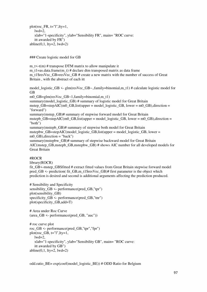
97
plot(roc_FR, t="l",lty=1, lwd=2, xlab="1-specificity", ylab="Sensibility FR", main= "ROC curve: itt awarded by FR") abline(0,1, lty=2, lwd=2) ### Create logistic model for GB m_t<-t(m) # transpose DTM matrix to allow manipulate it m_t1=as.data.frame(m_t) # declare dtm transposed matrix as data frame m_t1$resVec_GB=resVec_GB # create a new matrix with the number of success of Great Britain , with the abstract of each itt model_logistic_GB <- glm(resVec_GB~.,family=binomial,m_t1) # calculate logistic model for GB m0_GB=glm(resVec_GB~1,family=binomial,m_t1) summary(model_logistic_GB) # summary of logistic model for Great Britain mstep_GB=stepAIC(m0_GB,list(upper = model_logistic_GB, lower = m0_GB),direction = "forward") summary(mstep_GB)# summary of stepwise forward model for Great Britain mstepb_GB=stepAIC(m0_GB,list(upper = model_logistic_GB, lower = m0_GB),direction = "both") summary(mstepb_GB)# summary of stepwise both model for Great Britain mstepbw_GB=stepAIC(model_logistic_GB,list(upper = model_logistic_GB, lower = m0_GB),direction = "back") summary(mstepbw_GB)# summary of stepwise backward model for Great Britain AIC(mstep_GB,mstepb_GB,mstepbw_GB) # shows AIC number for all developed models for Great Britain #ROCR library(ROCR) fit_GB<-mstep_GB$fitted # extract fitted values from Great Britain stepwise forward model pred_GB <- prediction( fit_GB,m_t1$resVec_GB)# first parameter is the object which prediction is desired and second is additional arguments affecting the prediction produced. # Sensibility and Specificity sensibility_GB <- performance(pred_GB,"tpr") plot(sensibility_GB) specificity_GB <- performance(pred_GB,"tnr") plot(specificity_GB,add=T) # Area under Roc Curve (area_GB <- performance(pred_GB, "auc")) # roc curve plot roc_GB <- performance(pred_GB,"tpr","fpr") plot(roc_GB, t="l",lty=1, lwd=2, xlab="1-specificity", ylab="Sensibility GB", main= "ROC curve: itt awarded by GB") abline(0,1, lty=2, lwd=2) odd.ratio_BE= exp(coef(model_logistic_BE)) # ODD Ratio for Belgium

98
odd.ratio_DE= exp(coef(model_logistic_DE)) # ODD Ratio for Germany odd.ratio_FR= exp(coef(model_logistic_FR)) # ODD Ratio for France odd.ratio_GB= exp(coef(model_logistic_GB)) # ODD Ratio for Great Britain odd.ratio_IT= exp(coef(model_logistic_IT)) # ODD Ratio for Italy ################################################################################################################### # Export data for excel fit_DE<-as.data.frame(fit_DE) export(fit_DE, "file_DE.csv") fit_BE<-as.data.frame(fit_BE) export(fit_BE, "file_BE.csv") fit_FR<-as.data.frame(fit_FR) export(fit_FR, "file_FR.csv") fit_IT<-as.data.frame(fit_IT) export(fit_IT, "file_IT.csv") fit_GB<-as.data.frame(fit_GB) export(fit_GB, "file_GB.csv") odd.ratio_IT<-as.data.frame(odd.ratio_IT) export( odd.ratio_IT, "odd_IT.csv") odd.ratio_DE<-as.data.frame(odd.ratio_DE) export( odd.ratio_DE, "odd_DE.csv") odd.ratio_BE<-as.data.frame(odd.ratio_BE) export( odd.ratio_BE, "odd_BE.csv") odd.ratio_FR<-as.data.frame(odd.ratio_FR) export( odd.ratio_FR, "odd_FR.csv") odd.ratio_GB<-as.data.frame(odd.ratio_GB) export(odd.ratio_GB, "odd_GB.csv")

99
R code for clustering techniques require(XLConnect) # package for interface with excel require(stringr) # package for manipulation of characters, whitespace, length require(stringi) # package for manipulation of characters, whitespace, length require(ggplot2) # package for graphic manipulation and development require (stats) # package for statistics calculation and random number generation require(tabplot) require(aod) require(gtools) require(corrgram) require(ROCR) require(dplyr) require(broom) require(Hmisc) require(rio) require(tm) # package for text mining require(MASS) # permit stepwise in a logistic model require(WriteXLS) # export data from R to excel require(SnowballC) require(pRoc) # create ROC curve require(arules) # create discret variables require(cluster) require(dendextend) require(factoextra) require(mclust) require(utils) require(clValid)# cluster validation tools require(ggfortify) require(FactoMineR) require(survival) require(MASS) # Read the data file Winners_ESA_initial <- readWorksheetFromFile("data_ESA_2018.xlsx", sheet=1, startRow = 1, endCol = 16) # Extract the bidding country names from the winner field of the XLS file Countries.itt <- regmatches(Winners_ESA_initial$Winners,gregexpr("(?<=\\().*?(?=\\))",Winners_ESA_initial$Winners, perl=TRUE)) Countries.itt <- as.matrix(Countries.itt) # Prepare the vector with names of the bidding countries Country_Names <- unique(unlist(Countries.itt)) Country_Names <- Country_Names[order(Country_Names)] Country_Names <- as.matrix(Country_Names) # Prepare the vector with names of the ESA Offices ESA_Office_Per_ITT <- Winners_ESA_initial$ESA.Site ESA_Office <- unique(Winners_ESA_initial$ESA.Site) ESA_Office <- ESA_Office[order(ESA_Office)] # Create the counter matrix that will store the number of contracts by country and office numberOfCountries <- length(unique(Country_Names))

100
numberOfEsaOffices <- length(unique(ESA_Office)) CounterMatrix <- matrix(rep(0, times=(numberOfCountries*numberOfEsaOffices)), nrow=numberOfEsaOffices, ncol=numberOfCountries) # Now, ITT by ITT, fill the counter matrix adding +1 for each ITT at the position of # the country and ESA office that participated in the contract # There are faster ways to do this, but lets keep it simple and understandable for(i in 1:nrow(Winners_ESA_initial)) { # Extract the winner countries (can be more than one) and ESA offices (can be more than one) ITT_winnerCountry <- unlist( Countries.itt[i] ) ITT_contractEsaOffice <- unlist( ESA_Office_Per_ITT[i] ) # Add one to the counter matrix at the position of the country and ESA office for(idxCountry in 1:length(ITT_winnerCountry)) { for(idxEsaOffice in 1:length(ITT_contractEsaOffice)) { CounterMatrixCol <- which(Country_Names == ITT_winnerCountry[idxCountry]) CounterMatrixRow <- which(ESA_Office == ITT_contractEsaOffice[idxEsaOffice]) CounterMatrix[CounterMatrixRow, CounterMatrixCol] <- CounterMatrix[CounterMatrixRow, CounterMatrixCol] + 1 } } } # Normalization Total_per_Country <- apply(CounterMatrix, 2,sum) Total_per_ESA_Office <- apply(CounterMatrix, 1,sum) N_Countries <- apply(CounterMatrix, 1, function(x){x/Total_per_Country}) N_Office <- apply(CounterMatrix, 2, function(x){x/Total_per_ESA_Office}) # Creates the image plot for the normalization by country pdf("Distribution_norm_Country.pdf",width=16, height=8) Norm_Countries_plot_colours <- image((N_Countries),col=terrain.colors(100),yaxt = "n",xaxt = "n") axis(1,at=seq(0,1,length.out = length(Country_Names)), labels= Country_Names, lty=0) axis(2,at=seq(0,1,length.out = length(ESA_Office)), labels=ESA_Office, lty=0) dev.off() # Creates the image plot for the normalization by ESA Office pdf("Distribution_norm_Office.pdf",width=16, height=8) Norm_Offices_plot_colours <- image(t(N_Office),col=terrain.colors(100),yaxt = "n",xaxt = "n") axis(1,at=seq(0,1,length.out = length(Country_Names)), labels= Country_Names,lty=0) axis(2,at=seq(0,1,length.out = length(ESA_Office)), labels=ESA_Office,lty=0) dev.off() # Prepare the vector with names of the ESA Programme Names ESA_Program_Per_ITT <- Winners_ESA_initial$PROGRAMME.NAME ESA_Program <- unique(Winners_ESA_initial$PROGRAMME.NAME) ESA_Program <- ESA_Program[order(ESA_Program)] # Create the counter matrix that will store the number of contracts by country,office and Programme Names numberOfCountries <- length(unique(Country_Names)) numberOfEsaOffices <- length(unique(ESA_Office)) numberOfEsaProgram <- length(unique(ESA_Program))

101
CounterMatrix <- matrix(rep(0, times=(numberOfCountries*numberOfEsaProgram)), nrow=numberOfEsaProgram, ncol=numberOfCountries) # Now, ITT by ITT, fill the counter matrix adding +1 for each ITT at the position of # the country and Program that participated in the contract # There are faster ways to do this, but lets keep it simple and understandable for(i in 1:nrow(Winners_ESA_initial)) { # Extract the winner countries (can be more than one), and ESA Programme (can be more than one) ITT_winnerCountry <- unlist( Countries.itt[i] ) ITT_EsaProgramme <- unlist( ESA_Program_Per_ITT[i] ) # Add one to the counter matrix at the position of the country and Esa Programme for(idxCountry in 1:length(ITT_winnerCountry)) { for(idxEsaProgramme in 1:length(ITT_EsaProgramme)) { CounterMatrixCol <- which(Country_Names == ITT_winnerCountry[idxCountry]) CounterMatrixRow <- which(ESA_Program == ITT_EsaProgramme[idxEsaProgramme]) CounterMatrix[CounterMatrixRow, CounterMatrixCol] <- CounterMatrix[CounterMatrixRow, CounterMatrixCol] + 1 } } } # Normalization Total_per_Country<- apply(CounterMatrix, 2,sum) Total_per_ESA_Program <- apply(CounterMatrix, 1,sum) N_Countries <- apply(CounterMatrix, 1, function(x){x/Total_per_Country}) N_Program <- apply(CounterMatrix, 2, function(x){x/Total_per_ESA_Program}) # Creates the image plot for the normalization by Country and Program pdf("Distribution_norm_Country_per_Program.pdf", width= 14, height= 14) Norm_Countries_plot_colours <- image(t(N_Program),col=terrain.colors(32),yaxt = "n",xaxt = "n") axis(1,at=seq(0,1,length.out = length(Country_Names)), labels= Country_Names, lty=0) axis(2,at=seq(0,1,length.out = length(ESA_Program)), labels=(ESA_Program), lty=0) dev.off() data_with_Countries<-cbind(Winners_ESA_initial,Countries.itt) text_final<- data_with_Countries$ABSTRACT #take the abstract from each ESA ITT text_final<-stemDocument(text_final, language = "english") # mantain the root of each word text_final<-tolower(text_final) #convert the text in lower case stop_w<-stopwords("english")# create a vector with english stop words text_final<-removeWords(text_final,stop_w)# remove stopword from english language stop_w_dtm<- (c("activ","also","base","can","current","develop","esa","high","includ","level","new","oper","perform","process", "provid", "requir", "satellit", "servic", "shall", "space","support","system","technolog", "use","data","design","implement","studi","test","mission","procur","model","need","object","addit","inform","measur","smes","will","phase")) text_final<-removeWords(text_final,stop_w_dtm) text_final<-removePunctuation(text_final) # remove punctuations

102
text_final<-removeNumbers(text_final) # remove numbers text_final<-stripWhitespace(text_final) # remove extra white space text_final<-wordStem(text_final,language= "english") #mantain the primitive form of the word, not considering verbal times, plural and singular text_final<-c(text_final) # text_final as character text_corpus<- Corpus(VectorSource(c(text_final))) # create a corpus for the DTM. #The source for this DTM will be a vector extracted from the original database ( only abstract colum) dtm <- TermDocumentMatrix(text_corpus) # remove terms that occurs in 15% of the documents and mantain words that appears at least in 85% of the document dtm<-removeSparseTerms(dtm,0.85) m <- as.matrix(dtm) # declare DTM as matrix m_t<-t(m) #transporse matrix m dim(m_t) m_t[which(is.na(m_t), arr.ind=TRUE)] <- 0 #Cluster construction plot(hclust(dist(m_t))) # compute cluster using complete method # data preparation for correlation matrix set.seed(123) ss <- sample(1:757, 757) # Take 50 random rows, inside the 757 observations df <- m_t[ss,] # Subset of the 50 random rows df.scaled <- scale(df) #Computing correlation based distances dist.cor <- get_dist(df.scaled, method = "pearson") #Visualizing correlation matrices from all 757 observations fviz_dist(dist.cor) # Agglomerative Nesting (Hierarchical Clustering) agnes(m_t, metric = "euclidean", stand = FALSE, method = "average") # Compute agnes() res.agnes <- agnes(m_t, method = "complete") # Agglomerative coefficient res.agnes$ac pltree(res.agnes, cex = 0.6, hang = -1,main = "Dendrogram of agnes") # Compute diana() res.diana <- diana(m_t, metric = "euclidean") # Plot the tree pltree(res.diana, cex = 0.6, hang = -1,main = "Dendrogram of diana") # Divise coefficient; amount of clustering structure found res.diana$dc #define optimal cluster number

103
fviz_nbclust(df, kmeans, method = "silhouette", k.max = 30) + theme_classic() #optimal clustering number for Kmeans fviz_nbclust(df, pam, method = "silhouette", k.max = 20) + theme_classic() #optimal clustering number for PAM #non-hierarchical clustering cluster_itt_Kmeans<-kmeans(m_t, centers=5); cluster_itt_PAM<-pam(m_t, 4); fviz_cluster(list(data = m_t, cluster =cluster_itt_Kmeans$cluster )) fviz_cluster(list(data = m_t, cluster =cluster_itt_PAM$cluster )) # select the best method of clustering among the used in this thesis without PCA express <- m_t intern <- clValid(express, 2:20, clMethods = c("hierarchical","kmeans", "diana", "pam"), validation = "internal") summary(intern) #PCA clusters m_t_PCA<-prcomp(m_t, scale=TRUE)# PCA construction # Cluster number study, considering a certain number of dimensions nDimToConsider <- 10 fviz_nbclust(x=m_t_PCA$x[,1:nDimToConsider], FUNcluster=kmeans, method = "silhouette", k.max=25) # Clustering solution pp<-kmeans(m_t_PCA$x[,1:nDimToConsider], centers = 4) fviz_cluster(list(data=m_t, cluster=as.factor(pp$cluster)), labelsize=6, geom="point", pointsize=0.2, show.clust.cent=FALSE) # Lets see if there are word clusters with a larger fraction of contracts won by # certain countries or not... countries_winner<-data_with_Countries$Countries.itt countries_winner<-unlist(c(countries_winner)) # country winner as character nClusts <- length(unique(pp$cluster)) totWinner <- table(unlist(countries_winner)) myClustWinnerMat <- matrix(nrow=nClusts, ncol=length(totWinner)) for(i in 1:nClusts){ clNumb <- i clNumbWinner <- table( c(unlist(countries_winner[which(pp$cluster==clNumb)]), unique(unlist(countries_winner)) )) - 1 myClustWinnerMat[i,] <- clNumbWinner } myClustWinnerMat <- apply(myClustWinnerMat, 2, function(i) i/sum(i)) myClustWinnerMat[which(is.na(myClustWinnerMat), arr.ind=TRUE)] <- 0 colnames(myClustWinnerMat) <- names(clNumbWinner) # Here is the matrix with showing the percentage of contracts won by each country (each country adds to 100). print(round(myClustWinnerMat,3)*100) matrix_pca_cluster<-print(round(myClustWinnerMat,3)*100)

104
Answers from Space Agency and Space Offices, and ESA Procurement Department

18/10/2018 Laboratory for Systems, Instrumentation and Modeling in Science and Technology for Space and the Environment (SIM) Correio - I…
https://mail.google.com/mail/u/0?ik=b571eb6269&view=pt&search=all&permmsgid=msg-f%3A1614655166922003100&simpl=msg-f%3A1614655… 1/1
Izabella Hemprich <[email protected]>
Information - Austrian Space activities
Michaela Gitsch <[email protected]> 18 de outubro de 2018 às 10:32Para: Hemprich Izabella <[email protected]>
Dear Izabelle Hemprich, for more information about the Aeronautics and Space Agency of FFG please go to https://www.ffg.at/content/ihre-ansprechpartnerinnen-der-agentur-f-r-luft-und-raumfahrt best regards, Michaela Gitsch Agentur für Luft- und Raumfahrt Österreichische Forschungsförderungsgesellschaft mbH (FFG) Sensengasse 1 A-1090 Wien Tel +43 (0)5 7755-3302 Fax +43 (0)5 7755-97900 [email protected] www.ffg.at, www.ffg.at/alr *********************************************************************************************** Alle aktuellen Fördermöglichkeiten der FFG auf einen Blick https://www.ffg.at/foerderungen Besuchen Sie uns auch auf Facebook: www.facebook.com/ffg.forschungwirkt FFG Disclaimer / Legal notice: http://www.ffg.at/Disclaimer *********************************************************************************************** >>> Izabella Hemprich <[email protected]> 15.10.2018 14:20 [Citação ocultada]

18/10/2018 Ihre AnsprechpartnerInnen in der Agentur für Luft- und Raumfahrt | FFG
https://www.ffg.at/content/ihre-ansprechpartnerinnen-der-agentur-f-r-luft-und-raumfahrt 1/2
DE | ENHome Presse Jobs eCALL eNewsletter
Ihre AnsprechpartnerInnen in derAgentur für Luft- und Raumfahrt
Leiter der AgenturAndreas Geisler Tel +43 (0)5 7755-3001 andreas.geisler@�g.at
AdministrationDoris Wach Tel +43 (0)5 7755-3012 doris.wach@�g.at
Pamela Spork Tel +43(0)5 7755-3013 pamela.spork@�g.at
Education & OutreachMichaela Gitsch Tel +43 (0)5 7755-3302 michaela.gitsch@�g.at
IndustriepolitikElisabeth Kla�enböck Tel +43(0)5 7755-3311 elisabeth.kla�enboeck@�g.at
Stephan Mayer Tel. +43(0)5 7755-3305 stephan.mayer@�g.at
Galileo Contact Point Austria,SatellitennavigationMatthias Schreitl Tel +43 (0)5 7755-3306 matthias.schreitl@�g.at
Stephan Mayer Tel +43 (0)5 7755-3305 stephan.mayer@�g.at
Telekommunikation / ErdbeobachtungLuc Berset Tel +43 (0)5 7755-3308 luc.berset@�g.at
Thomas Geist Tel +43 (0)5 7755-3310 thomas.geist@�g.at
Weltraumwissenschaften, BemannteRaumfahrt, Robotische Exploration,Weltraumtransportsysteme
Weitere Informationen
Agentur für Luft- und Raumfahrt
der FFG
Startseite › Ihre AnsprechpartnerInnen in der Agentur für Luft- und RaumfahrtSuche...
Förderungen suchen
Förderung suchen
ProjektdatenbankKurzinfos zu geförderten Projekten
eCallMeine Projekte abwickeln und verwalten
FörderpilotBundes- und Landesförderungen auf einen
Klick
Ich suche (Thema)
Ich suche (Zielgruppe)
nationale Förderungen
internationale Förderungen
Die FFG Förderungen Services Informationen
Cookies helfen uns bei der Bereitstellung unserer Dienste. Durch die Nutzung unserer Dienste erklären Sie sich damit einverstanden, dass wir Cookies setzen. Weitere Informationen Ok

18/10/2018 Ihre AnsprechpartnerInnen in der Agentur für Luft- und Raumfahrt | FFG
https://www.ffg.at/content/ihre-ansprechpartnerinnen-der-agentur-f-r-luft-und-raumfahrt 2/2
Andre Peter Tel +43 (0)5 7755-3309 andre.peter@�g.at
Österreichisches Weltraumprogramm ASAPLudwig Hofer Tel + 43(0)5 7755-3301 ludwig.hofer@�g.at
European Space Policy Institute (ESPI)Wolfgang Würz tel +43 (0)1 718 111-811 [email protected]
Artikelfunktionen
Empfehlen & Weiterleiten
Die FFG
Ziele und Aufgaben
Organisation
MitarbeiterInnen-Verzeichnis
Kontakt und Anreise
Förderungen
Alle Förderprogramme
Themenschwerpunkte
Angebote für Jugendliche
Angebote für Start-ups
Angebote für KMU
EU-Programm Horizon 2020
Förderbedingungen
eCall – Projektabwicklung
Services
QuickCheck
Gutachten Forschungsprämie
Jobbörse für Forschung
Praktika für Jugendliche
Beratung
Partnersuche
Schulung und Training
Rechtliche Services
Technologietransfer
Innovationsfördernde ö�entliche
Bescha�ung
EU-Performance Monitoring
EURAXESS – Karrierechancen in
Europa
Informationen
News
o�ene Ausschreibungen
Veranstaltungen
eNewsletter
Publikationen und Berichte
FFG auf Facebook
Abkürzungsverzeichnis
Glossar
Die Österreichische Forschungsförderungsgesellschaft FFG steht im Eigentum der Republik Österreich. Eigentümervertreter sind das Bundesministerium für Digitalisierung undWirtschaftsstandort und das Bundesministerium für Verkehr, Innovation und Technologie
Copyright © 2005 - 2018 FFG - Die Österreichische Forschungsförderungsgesellschaft. All rights reserved. Worldwide.
Home · Impressum · Kontakt · Sitemap · Datenschutz

24/10/2018 Laboratory for Systems, Instrumentation and Modeling in Science and Technology for Space and the Environment (SIM) Correio - …
https://mail.google.com/mail/u/0?ik=b571eb6269&view=pt&search=all&permmsgid=msg-f%3A1615216279031401930&simpl=msg-f%3A1615216… 1/2
Izabella Hemprich <[email protected]>
RE: General information : Information Canada Space Agency
Info (ASC/CSA) <[email protected]> 24 de outubro de 2018 às 15:11Para: "[email protected]" <[email protected]>
Good day,
Thank you for contacting the Canadian Space Agency (CSA).
Please note that the CSA has approximately 670 employees. You may visit our website for more information.
Best regards,
Service à la clientèle | Communications et affaires publiques
Agence spatiale canadienne | Gouvernement du Canada
[email protected] | Tél. : 450-926-4351
Customer Service | Communications and Public Affairs
Canadian Space Agency | Government of Canada
[email protected] | Tel. : 450-926-4351
Fro : [email protected] <[email protected]> Se t: O to er-1 -1 : AM To: I fo ASC/CSA <[email protected]> Su je t: Ge eral i for a�o : I for a�o Ca ada Spa e Age y
Canadian Space Agency
Information request form
General information
Information Canada Space Agency
Message Dear Sir or Madam, I´m a research engineer and now i´m finishing my master thesis in applied mathematics. My tesis is a study regarding how ESA ITT´s is correlated with countries, expertises and othervariables. I´m studying all ITT´s since 2013. Now, I´m studying how ESA awarded ITTs are correlated with the number of human resources thateach space office has. I want to ask you, if is it possible to provide me oficial information regarding the number of CanadaSpace Agency employees? If you have any doubt, please feel free to contact me. With best regards, -- Izabella Hemprich Control Engineer and Msc Student in Applied Mathematics FCUL,CENTRA-SIM group
Date/Time
Sent on Sunday, October 14, 2018 at9:38
Communications
Canadian citizen No
Further details Yes
Send me a response Yes
Contact info
Name Izabella Hemprich
E-mail [email protected]

24/10/2018 Laboratory for Systems, Instrumentation and Modeling in Science and Technology for Space and the Environment (SIM) Correio - …
https://mail.google.com/mail/u/0?ik=b571eb6269&view=pt&search=all&permmsgid=msg-f%3A1615216279031401930&simpl=msg-f%3A1615216… 2/2
email: [email protected] skype: izabella_hemprich phone: 351 217500000 - ext: 28136 FCUL web site: http://www.fc.ul.pt/ CENTRA-SIM web site: http://centra.tecnico.ulisboa.pt/network/sim/
Home phone 351-915-5289
Work phone 351-217-5000 #28136

17/10/2018 Laboratory for Systems, Instrumentation and Modeling in Science and Technology for Space and the Environment (SIM) Correio - I…
https://mail.google.com/mail/u/0?ik=b571eb6269&view=pt&search=all&permmsgid=msg-f%3A1614583786968480230&simpl=msg-f%3A1614583… 1/1
Izabella Hemprich <[email protected]>
Information regarding Space business in Denmark
office <[email protected]> 17 de outubro de 2018 às 15:35Para: Izabella Hemprich <[email protected]>
Hi Iza ella
At DTU Spa e Na�o al Spa e I s�tute, Te h i al U i ersity of De ark e are 5 e ployees.
Ki d regards,
Lene Bettenhaus
Ledelsessekretær
DTU Space
Danmarks Tekniske Universitet
Institut for Rumforskning og Rumteknologi
Elektrovej
Bygning 328, Rum 132
2800 Kgs. Lyngby
Direkte telefon 45259502
www.dtu.dk
Fra: Izabella Hemprich [mailto:[email protected]] Sendt: 15. oktober 2018 15:30 Til: office Emne: Re: Information regarding Space business in Denmark
[Citação ocultada]

25/10/2018 Laboratory for Systems, Instrumentation and Modeling in Science and Technology for Space and the Environment (SIM) Correio - I…
https://mail.google.com/mail/u/0?ik=b571eb6269&view=pt&search=all&permmsgid=msg-f%3A1615303042614170386&dsqt=1&simpl=msg-f%3A… 1/4
Izabella Hemprich <[email protected]>
Information regarding Space business in Denmark
office <[email protected]> 25 de outubro de 2018 às 14:06Para: Izabella Hemprich <[email protected]>
Hi
No De ark do ot ha e a Spa e Age y.
We are u der the Da ish Go er e t.
Da ish Age y for S ie e a d Higher Edu a�o : [email protected]
Ki d regards,
Lene Bettenhaus
Ledelsessekretær
DTU Space
Danmarks Tekniske Universitet
Institut for Rumforskning og Rumteknologi
Elektrovej
Bygning 328, Rum 132
2800 Kgs. Lyngby
Direkte telefon 45259502
www.dtu.dk
Fra: Izabella Hemprich [mailto:[email protected]] Sendt: 23. oktober 2018 17:02 Til: office Emne: Re: Information regarding Space business in Denmark
Dear Lene,
Thank you again for answering my question.
I have one doubt about Denmark space organization.
Can you please help me?
I want to know, if is there a danish space agency or a danish space office?

25/10/2018 Laboratory for Systems, Instrumentation and Modeling in Science and Technology for Space and the Environment (SIM) Correio - I…
https://mail.google.com/mail/u/0?ik=b571eb6269&view=pt&search=all&permmsgid=msg-f%3A1615303042614170386&dsqt=1&simpl=msg-f%3A… 2/4
With my best regards,
Izabella
office <[email protected]> escreveu no dia quarta, 17/10/2018 à(s) 15:38:
Hi Iza ella
At DTU Spa e Na�o al Spa e I s�tute, Te h i al U i ersity of De ark e are 5 e ployees.
Ki d regards,
Lene Bettenhaus
Ledelsessekretær
DTU Space
Danmarks Tekniske Universitet
Institut for Rumforskning og Rumteknologi
Elektrovej
Bygning 328, Rum 132
2800 Kgs. Lyngby
Direkte telefon 45259502
www.dtu.dk
Fra: Izabella Hemprich [mailto:[email protected]] Sendt: 15. oktober 2018 15:30 Til: office Emne: Re: Information regarding Space business in Denmark
Dear Lene Bettenhaus,
Thank you for the answer.
I just want to know about your institute, DTU Space.
With kind regards,
Izabella

25/10/2018 Laboratory for Systems, Instrumentation and Modeling in Science and Technology for Space and the Environment (SIM) Correio - I…
https://mail.google.com/mail/u/0?ik=b571eb6269&view=pt&search=all&permmsgid=msg-f%3A1615303042614170386&dsqt=1&simpl=msg-f%3A… 3/4
office <[email protected]> escreveu no dia segunda, 15/10/2018 à(s) 14:23:
Dear Iza ella
If you eed the total u er of e ployees i De ark orki g o spa e progra s you eed to o ta t our Mi istry.
There are se eral fir s a d i s�tutes.
If you o ly eed the u er fro our i s�tute, DTU Spa e, please let e k o .
Ki d regards,
Lene Bettenhaus
Ledelsessekretær
DTU Space
Danmarks Tekniske Universitet
Institut for Rumforskning og Rumteknologi
Elektrovej
Bygning 328, Rum 132
2800 Kgs. Lyngby
Direkte telefon 45259502
www.dtu.dk
Fra: Izabella Hemprich [mailto:[email protected]] Sendt: 15. oktober 2018 14:39 Til: office Emne: Information regarding Space business in Denmark
Dear Sir or Madam, I´m a research engineer and now i´m finishing my master thesis in applied mathematics. My tesis is a study regarding how ESA ITT´s is correlated with countries, expertises and other variables. I´m studying all ITT´s since 2013. Now, I´m studying how ESA awarded ITTs are correlated with the number of human resources that each space office has. I want to ask you, if is it possible to provide me oficial information regarding the number of employees are working full time for Space programs inDenmark ( Can be the number of employees you have at your space office)? If you have any doubt, please feel free to contact me. With best regards, --
Izabella Hemprich
Control Engineer and Msc Student in Applied Mathematics
FCUL,CENTRA-SIM group
email: [email protected]

25/10/2018 Laboratory for Systems, Instrumentation and Modeling in Science and Technology for Space and the Environment (SIM) Correio - I…
https://mail.google.com/mail/u/0?ik=b571eb6269&view=pt&search=all&permmsgid=msg-f%3A1615303042614170386&dsqt=1&simpl=msg-f%3A… 4/4
skype: izabella_hemprich
phone: 351 217500000 - ext: 28136
FCUL web site: http://www.fc.ul.pt/
CENTRA-SIM web site: http://centra.tecnico.ulisboa.pt/network/sim/
--
Izabella Hemprich
Control Engineer and Msc Student in Applied Mathematics
FCUL,CENTRA-SIM group
email: [email protected]
skype: izabella_hemprich
phone: 351 217500000 - ext: 28136
FCUL web site: http://www.fc.ul.pt/
CENTRA-SIM web site: http://centra.tecnico.ulisboa.pt/network/sim/
--
Izabella Hemprich
Control Engineer and Msc Student in Applied Mathematics
FCUL,CENTRA-SIM group
email: [email protected]
skype: izabella_hemprich
phone: 351 217500000 - ext: 28136
FCUL web site: http://www.fc.ul.pt/
CENTRA-SIM web site: http://centra.tecnico.ulisboa.pt/network/sim/

15/10/2018 Laboratory for Systems, Instrumentation and Modeling in Science and Technology for Space and the Environment (SIM) Correio - …
https://mail.google.com/mail/u/0?ik=b571eb6269&view=pt&search=all&permmsgid=msg-f%3A1614400005739424263&simpl=msg-f%3A1614400… 1/2
Izabella Hemprich <[email protected]>
RE: Information regarding Space business in Estonia
Tiiu Treier <[email protected]> 15 de outubro de 2018 às 14:56Para: "[email protected]" <[email protected]>
Dear Iza ella He pri h
We ha e t o FTE at the Spa e Offi e i Esto ia. You a fi d a short o er ie of us fro here https://www.eas.ee/teenus/estonian-space-office/?lang=en.
Best regards
Tiiu Treier
Proje t Ma ager
Trade De elop e t Age y
E terprise Esto ia
Las a äe , , Talli , Esto ia
Mo : +
Tel: +
www.eas.ee
www.facebook.com/EnterpriseEstonia
https://www.eas.ee/teenus/estonian-space-office/?lang=en
Fro : Iza ella He pri h <[email protected]> Se t: Mo day, O to er , : PM To: I fo eas <[email protected]> Su je t: I for a�o regardi g Spa e usi ess i Esto ia
Dear Sir or Madam, I´m a research engineer and now i´m finishing my master thesis in applied mathematics. My thesis is a study regarding how ESA ITT´s is correlated with countries, expertises and other variables. I´m studying all ITT´s since 2013. Now, I´m studying how ESA awarded ITTs are correlated with the number of human resources that each space office has. I want to ask you, if is it possible to provide me official information regarding the number of employees are working full time for Space programs inEstonian Space Office? If you have any doubt, please feel free to contact me. With best regards, --

15/10/2018 Laboratory for Systems, Instrumentation and Modeling in Science and Technology for Space and the Environment (SIM) Correio - …
https://mail.google.com/mail/u/0?ik=b571eb6269&view=pt&search=all&permmsgid=msg-f%3A1614400005739424263&simpl=msg-f%3A1614400… 2/2
Izabella Hemprich
Control Engineer and Msc Student in Applied Mathematics
FCUL,CENTRA-SIM group
email: [email protected]
skype: izabella_hemprich
phone: 351 217500000 - ext: 28136
FCUL web site: http://www.fc.ul.pt/
CENTRA-SIM web site: http://centra.tecnico.ulisboa.pt/network/sim/

15/10/2018 Estonian Space Office - EAS
https://www.eas.ee/teenus/estonian-space-office/?lang=en 1/2
Monday 15th of October 2018. 02:04:10 PMhttp://www.eas.ee/teenus/estonian-space-o�ice/?lang=en
Estonian Space O�ice Eesti Kosmosebüroo (https://www.eas.ee/teenus/eesti-kosmoseburoo/?lang=et)
Enterprise Estonia is the developer of the Estonian space policy and space business, and it promotes international cooperation, providing Estonian companies withnew business opportunities on markets contributing to high technology. Estonia has been a full member of the European Space Agency (ESA) since 2015. Estonian Space o�ice:
Enterprise Estonia does not financially support the preparation of projects.
Estonian companies operating in the field of space can be found here: https://estonia.ee/companies-tags/smart-space-technology-and-applications/(https://estonia.ee/companies-tags/smart-space-technology-and-applications/)
Information on how to create a company in Estonia can be found here: https://e-resident.gov.ee/ (https://e-resident.gov.ee/)
ParticipationTo participate in the programme, please contact the Estonian Space O�ice
Madis Võõras [email protected] (mailto:[email protected]) 627 9795
Tiiu Treier [email protected] (mailto:[email protected]) 6279404
Target group: Estonian companies having competence, motivation, and capability (including start-up companies).Open
mediates the invitations to tender of ESA (Participation in the invitations to tender of ESA enables Estonian companies and research institutions to successfully participate in the European Space Agency projects,
thereby helping to bring new high-tech jobs to Estonia. It also creates prerequisites for the development of science-intensive products and services with high added value that
are internationally competitive.)
consults the project developers
organises information days, seminars, conferences, study trips, and match-making events
Goal
Results
To contribute to the readiness of Estonian companies and research institutions to participate in theinvitations to tender of ESA, and to be successful in institutional export.
The volume of contracts related to the space sector increases by 20% per year.

15/10/2018 Estonian Space Office - EAS
https://www.eas.ee/teenus/estonian-space-office/?lang=en 2/2

23/10/2018 Laboratory for Systems, Instrumentation and Modeling in Science and Technology for Space and the Environment (SIM) Correio - …
https://mail.google.com/mail/u/0?ik=b571eb6269&view=pt&search=all&permmsgid=msg-f%3A1615126043111838065&simpl=msg-f%3A1615126… 1/2
Izabella Hemprich <[email protected]>
RE: Mail du site cnes.fr
contact_cnes.fr <[email protected]> 23 de outubro de 2018 às 15:17Para: Hemprich <[email protected]>
Dear Mada ,
Tha k you for the i terest i our we site a d i our o pa y.
You a fi d these figures i our a ual report , at this address o our we site : https://cnes.fr/fr/le-cnes/le-cnes-en-bref/rapport-annuel-2017
Best regards,
Direction de la Communication
18 avenue Edouard Belin 31401 Toulouse Cedex 9
cnes.fr
De : He pri h <[email protected]> Envoyé : di a he 4 o to re : 4 Objet : Mail du site cnes.fr
Soumis le Dimanche, 14 Octobre, 2018 - 16:04 Soumis par l'utilisateur : Contenu du message : Vous
Nom Hemprich
Prénom Izabella
Adresse FCUL -Campo Grande - Edificio C8-Piso 1- Gabinete 36-Departamento de Física
Code postal 1749-016
Ville Lisboa
Pays Portugal
Email [email protected]
Contenu de votre message
Votre commentaire concerne Rubrique "Le CNES"
Votre commentaire concerne en particulier la page (Url) http://centra.tecnico.ulisboa.pt/network/sim/
Message
Dear Sir or Madam, I´m a research engineer and now i´m finishing my master thesis in applied mathematics. My tesis is a study regarding how ESA ITT´s is correlated with countries, expertises and other variables. I´m studying all ITT´s since 2013. Now, I´m studying how ESA awarded ITTs are correlated with the number of human resources that each space office has.

23/10/2018 Laboratory for Systems, Instrumentation and Modeling in Science and Technology for Space and the Environment (SIM) Correio - …
https://mail.google.com/mail/u/0?ik=b571eb6269&view=pt&search=all&permmsgid=msg-f%3A1615126043111838065&simpl=msg-f%3A1615126… 2/2
I want to ask you, if is it possible to provide me oficial information regarding the number of French Space Agency employees? If you have any doubt, please feel free to contact me. With best regards, -- Izabella Hemprich Control Engineer and Msc Student in Applied Mathematics FCUL,CENTRA-SIM group email: [email protected] skype: izabella_hemprich phone: 351 217500000 - ext: 28136 FCUL web site: http://www.fc.ul.pt/ CENTRA-SIM web site: http://centra.tecnico.ulisboa.pt/network/sim/

ANNUAL REPORT 2017RAPPORT D’ACTIVITÉ 2017

M I S S I O N R E C R U T E RR E C R U I T M E N T
UNE POLITIQUE RH D’EXCELLENCE
THE PURSUIT OF EXCELLENCE
Femmes / Womendont 27 en CDI27 on long-term contracts
Hommes / Mendont 61 en CDI61 on long-term contracts
32
66
Total dont 88 en CDI
Total88 on long-term
contracts
98
92
42
Cadre / Executive dont 82 en CDI82 on long-term contracts
Secrétaire SecretaryTechnicien
Technician
Totaldont 88 en CDI
Total88 on long-term
contracts
98
94%des recrutements concernent
des Ingénieurs et cadres.
Of new hires are engineers and executives.
2 386,1 Effectif moyen en équivalent
temps plein (ETP)
Mean headcount, full-time equivalent (FTE).
LES RECRUTEMENTS 2017 / Recruitment in 2017
Le CNES s’appuie sur près 2 500 femmes et hommes dont les compétences sont forgées par l’excellence et le partage de valeurs
communes, ainsi que sur un fort engagement social et environnemental. Parmi eux, une majorité d’ingénieurs et cadres (70 %) et de femmes (37 %). Cette politique se fonde sur une gestion des ressources humaines privilégiant la mobilité interne et la formation, afin d’accroître et d’optimiser les compétences de chacun. Elle met en œuvre des principes éthiques et de bonne gouvernance : développement d’un management responsable, promotion de la diversité et de la mixité, meilleure articulation entre vie professionnelle et vie personnelle et maintien d’un bon niveau de dialogue social.
!e lifeblood of CNES is the 2,500 people whose talents are forged by excellence and shared values, together with a strong social and environmental commitment. Of these, 70% are engineers and executives, and 37% are women. !e agency’s human resources strategy is based on a management approach fostering internal mobility and training in order to increase and optimize our skills base. It applies the principles of ethical b u s i n e s s c o n d u c t a n d g o o d governance, through a responsible management approach, promotion of diversity and gender balance, an optimized work-life balance and a high level of social dialogue.
Pauline Leblan,Correspondante Ressources
humaines, Siège du CNES à ParisHuman Resources correspondent,
CNES Head Office, Paris
« C’est à l’occasion de la réorganisation de la Direction des Ressources
Humaines début 2017 que j’ai été embauchée. Diplômée d’un Master 2 en Ressources Humaines, mes 8 ans d’expérience sur des missions RH opérationnelles et notamment en
mobilité interne, ont intéressé le CNES pour lequel j’avais déjà fait une période
d’intérim sur le même poste que j’occupe actuellement. J’accompagne les collaborateurs et managers de trois
directions fonctionnelles du CNES dans l’évolution de leur parcours
professionnel et les aide à développer leurs compétences. J’ai un rôle
de conseil et d’orientation aux côtés des collaborateurs qui cherchent à
changer de service ou de lieu de travail ou qui sont encouragés à le faire. »
“I was hired at the start of 2017 when the Human Resources directorate was reorganized. My Master’s 2 degree in Human Resources and eight years’
experience working on operational HR missions, focused notably on internal
mobility, interested CNES where I’d already completed a temp assignment in the same post
I occupy now. I help employees and managers in the agency’s three functional directorates to manage
their careers and develop their skills. My role is to advise and guide employees who are looking to
or being encouraged to change jobs or their place of work.”
58

26/10/2018 Laboratory for Systems, Instrumentation and Modeling in Science and Technology for Space and the Environment (SIM) Correio - …
https://mail.google.com/mail/u/0?ik=b571eb6269&view=pt&search=all&permmsgid=msg-f%3A1615386024384429514&simpl=msg-f%3A1615386… 1/1
Izabella Hemprich <[email protected]>
DLR personnel figures
[email protected] <[email protected]> 26 de outubro de 2018 às 12:09Para: [email protected]
Dear Ms Hemprich, here are the figures (as of September 2017) that might be of interest for you: Total number of employees: 8.127 (2.587 female) Non-scientific staff: 3.404 (50.7 % female) Scientific staff: 4.723 (18.2 % female) Average age: 40 years PhD candidates: 969 Trainees: 237 Student interns: 440 Best regards Daniel Beckmann —————————————————————————— Deutsches Zentrum für Luft- und Raumfahrt e.V. (DLR) German Aerospace Center Public Affairs and Communications | Linder Hoehe | 51147 Cologne | Germany Daniel Beckmann | Editor Digital Media | Corporate Design Telephone +49 2203 601-2466 | Mobile +49 174 3270300 | [email protected] DLR.de -----Ursprüngliche Nachricht----- Von: [email protected] [mailto:[email protected]] Gesendet: Freitag, 26. Oktober 2018 12:43 An: Mittelbach, Elisabeth Betreff: Allgemein IP : 172.21.177.129 Ursprungs-URL: https://www.dlr.de/rd/desktopdefault.aspx/tabid-2096/ subject : Allgemein Betreff : Information about DLR Nachricht : Dear Sir or Madam, I already sent this form about 2 weeks ago, and didn´t receive an answer. Sorry for send again the same question. " I´m a research engineer and now i´m finishing my master thesis in applied mathematics. My thesis is a study regarding how ESA ITT´s is correlated with countries, expertises and other variables. I´m studying all ITT´s since 2013. Now, I´m studying how ESA awarded ITTs are correlated with the number of human resources that each space office has. I want to ask you, if is it possible to provide me oficial information regarding the number of DLR employees? If you have any doubt, please feel free to contact me. With best regards, -- Izabella Hemprich Control Engineer and Msc Student in Applied Mathematics FCUL,CENTRA-SIM group email: [email protected] skype: izabella_hemprich phone: 351 217500000 - ext: 28136 FCUL web site: http://www.fc.ul.pt/ CENTRA-SIM web site: http://centra.tecnico.ulisboa.pt/network/sim/ Vorname : Izabella Name : Hemprich Email : [email protected] chkAgree : yes

23/10/2018 Laboratory for Systems, Instrumentation and Modeling in Science and Technology for Space and the Environment (SIM) Correio - …
https://mail.google.com/mail/u/0?ik=b571eb6269&view=pt&search=all&permmsgid=msg-f%3A1615034247895332208&dsqt=1&simpl=msg-f%3A… 1/1
Izabella Hemprich <[email protected]>
RE: Contact Us Request Received: - Information about Irish Space Office
Tony McDonald <[email protected]> 22 de outubro de 2018 às 14:57Para: "[email protected]" <[email protected]>
Dear Izabella
To respond to your request , at present there is no formal space office in Ireland. Responsibilities for ESA membership and associated space activities arecurrently primarily dealt with by the Department of Business Enterprise and Innovation (DBEI) and Enterprise Ireland. The number of individuals engaged in theseactivities, between the two organizations is 5. However these individuals may allocate some of their time to non ESA/Space activities, from time to time
I hope this answers your question
Best Regards
Tony
From: NicantSithigh, Aisling Sent: Monday 15 October 2018 14:35 To: [email protected] Cc: McDonald, Tony <[email protected]> Subject: RE: Contact Us Request Received: - Information about Irish Space Office
Thank you for your email which I am forwarding to Tony McDonald
Regards / le dea-mhéin
Aisling nic an tSithigh
e-mail / ríomhphost [email protected]
www.enterprise-ireland.com
The Plaza / East Point Business Park / Dublin 3 / Ireland
An Plaza / Páirc Ghnó Na Rinne Thoir / BAC 3 / Eireann
From: [email protected] <[email protected]> Sent: Monday 15 October 2018 14:12 To: Client Service <[email protected]> Cc: NicantSithigh, Aisling <[email protected]> Subject: Contact Us Request Received: - Information about Irish Space Office
Contact Us Request Received
Name: Izabella Hemprich
Email: [email protected]
Phone: (351)915528921
Comment: I´m a research engineer and now i´m finishing my master thesis in applied mathematics. My thesis is a study regarding how ESA ITT´s is correlated withcountries, expertises and other variables. I´m studying all ITT´s since 2013. Now, I´m studying how ESA awarded ITTs are correlated with the number of humanresources that each space office has. I want to ask you, if is it possible to provide me official information regarding the number of employees are working full time forSpace programs in Irish Space Office? If you have any doubt, please feel free to contact me. With best regards, -- Izabella Hemprich Control Engineer and MscStudent in Applied Mathematics FCUL,CENTRA-SIM group email: [email protected] skype: izabella_hemprich phone: 351 217500000 - ext: 28136FCUL web site: http://www.fc.ul.pt/ CENTRA-SIM web site: http://centra.tecnico.ulisboa.pt/network/sim
Processed: 15/10/2018 14:12:12
This email may contain information which is confidential and/or privileged. The information is intended solely for the use of the individual or entity named above. Ifyou are not the intended recipient, be aware that any disclosure, copying, distribution or use of the contents is prohibited. If you have received this electronictransmission in error, please notify the sender by telephone or return email and delete the material from your computer. Enterprise Ireland Tel: +353 (0) 1 7272000Web: www.enterprise-ireland.com *********************************************************** This email message has been scanned for viruses.***********************************************************

16/10/2018 Laboratory for Systems, Instrumentation and Modeling in Science and Technology for Space and the Environment (SIM) Correio - I…
https://mail.google.com/mail/u/0?ik=b571eb6269&view=pt&search=all&permthid=thread-a%3Ar4792028929650736996&simpl=msg-a%3Ar-5163… 1/2
Izabella Hemprich <[email protected]>
Information regarding ASI 3 mensagens
Izabella Hemprich <[email protected]> 14 de outubro de 2018 às 14:53Para: [email protected]
Dear Sir or Madam, I´m a research engineer and now i´m finishing my master thesis in applied mathematics.My tesis is a study regarding how ESA ITT´s is correlated with countries, expertises and other variables.I´m studying all ITT´s since 2013.Now, I´m studying how ESA awarded ITTs are correlated with the number of human resources that each space office has.I want to ask you, if is it possible to provide me oficial information regarding the number of Italian Space Agency employees?If you have any doubt, please feel free to contact me. With best regards, -- Izabella HemprichControl Engineer and Msc Student in Applied Mathematics FCUL,CENTRA-SIM groupemail: [email protected]: izabella_hemprichphone: 351 217500000 - ext: 28136FCUL web site: http://www.fc.ul.pt/CENTRA-SIM web site: http://centra.tecnico.ulisboa.pt/network/sim/
URP <[email protected]> 16 de outubro de 2018 às 08:18Para: Izabella Hemprich <[email protected]>
Dear Iza ella,
ASI e ployees are .
You a fi d useful i for a�o o this topi o our Trie ial A �vity Pla , here: https://www.asi.it/sites/default/files/attach/dettaglio/022_-_pta_2017-2019_-_pta_2017-2019_finale2.pdf, pages - .
We are sorry, ut this pla i s o ly i Italia .
Ki d regards,
ASI Pu li Rela�o s Offi e
Agenzia Spaziale Italiana
Unità Relazioni Esterne e URP
Via del Politecnico snc - 00133 Roma
Tel. +39 06 8567 237 Fax +39 06 8567 322
E-mail: [email protected] PEC: [email protected]
Web: www.asi.it www.asitv.it

16/10/2018 Laboratory for Systems, Instrumentation and Modeling in Science and Technology for Space and the Environment (SIM) Correio - I…
https://mail.google.com/mail/u/0?ik=b571eb6269&view=pt&search=all&permthid=thread-a%3Ar4792028929650736996&simpl=msg-a%3Ar-5163… 2/2
Facebook: www.facebook.com/agenziaspazialeitaliana
Twitter: www.twitter.com/ASI_spazio
Da: Iza ella He pri h <[email protected]> Inviato: do e i a o�o re : A: URP <[email protected]> Ogge�o: I for a�o regardi g ASI
[Citação ocultada]
Izabella Hemprich <[email protected]> 16 de outubro de 2018 às 10:40Para: [email protected]
Dear All, Thank you very much for the information!It is very important for my thesis.No problem the document is in italian! With kind regards, Izabella[Citação ocultada] 2 anexos
image001.jpg 7K
image001.jpg 7K

17/10/2018 Laboratory for Systems, Instrumentation and Modeling in Science and Technology for Space and the Environment (SIM) Correio - I…
https://mail.google.com/mail/u/0?ik=b571eb6269&view=pt&search=all&permmsgid=msg-f%3A1614559155064965978&simpl=msg-f%3A1614559… 1/1
Izabella Hemprich <[email protected]>
Information Polish Space Agency
Urszula Szwed-Strych <[email protected]> 17 de outubro de 2018 às 09:06Para: "[email protected]" <[email protected]>Cc: Sekretariat <[email protected]>
Dear Ms Hemprich,
thank you for your interest in POLSA.
Responding to your question - the Polish Space Agency currently employs 48 people.
Should you have any more questions regarding POLSA please do not hestitate to contact me directly.
Z poważaniem/
Best regards
Urszula Szwed-Strych
Główny Specjalista ds. Kontaktów z Mediami/
Chief Specialist for Media Relations
tel.: +48 516 222 671
tel.: +48 22 380 01 51
Polska Agencja Kosmiczna
ul. Trzy Lipy 3
80-172 Gdańsk
Oddział Terenowy w Warszawie
ul. Powsińska 69/71
02-903 Warszawa
NIP: 957-107-74-43
REGON: 360992221
www.polsa.gov.pl
Facebook/PolskaAgencjaKosmicznaPOLSA
--------------------------------------------------------------------------------------------------------------------------------------------------------------------------------
Treść tej wiadomości, wraz z ewentualnymi załącznikami, zawiera informacje przeznaczone tylko dla wymienionego w niej adresata i może zawierać informacje, które są poufne oraz prawnie chronione. Jeżeli nie są Państwo jej adresatem, bądź otrzymali ją przez pomyłkę należy: powiadomić niezwłocznie nadawcę poprzez odesłanie zwrotnej odpowiedzi na tę wiadomość, usunąć wiadomość w całości, nie ujawniać, nie rozpowszechniać, nie powielać i nie używać jej w jakikolwiek sposób w całości lub w części w jakiejkolwiek formie.
Fro : Iza ella He pri h [mailto:[email protected]] Se t: Su day, O to er , 8 : PM To: Sekretariat <[email protected]> Su je t: I for a�o Polish Spa e Age y
[Citação ocultada]

26/10/2018 Laboratory for Systems, Instrumentation and Modeling in Science and Technology for Space and the Environment (SIM) Correio - F…
https://mail.google.com/mail/u/0?ik=b571eb6269&view=pt&search=all&permmsgid=msg-f%3A1615383159392477150&simpl=msg-f%3A1615383… 1/1
Izabella Hemprich <[email protected]>
Fwd: Information about INTA
José Gabriel Carrión Martín <[email protected]> 26 de outubro de 2018 às 11:23Para: Izabella Hemprich <[email protected]>
Dea M s. He p i h,
So y fo ot ha i g a s e ed efo e.
A out you o sulta�o , u e t u e of INTA e ployees is a ou d , ut ot all of the a e s ie �fi -te h i al de oted. Roughly speaki g, ofthe a e dedi ated to di e t s ie �fi -te h i al a � i�es.
I hope I had a s e ed you ues�o .
Best ega ds,
José G. Carrión
INTA - Spanish Ministry of Defence
Area for Scientifical, Technical and Commercial Cooperation
De: Iza ella He p i h [ ailto:[email protected]] Enviado el: do i go, 4 de o tu e de 8 6: Para: José Ga iel Ca ió Ma � Asunto: F d: I fo a�o a out INTA
[Citação ocultada]


