Abstract—Motorway traffic management and control relies

on models that estimate and predict traffic conditions. In this

paper, a methodology for the identification and short-term

prediction of the traffic state is presented. The methodology

combines model-based clustering, variable-length Markov

chains and nearest neighbor classification. An application of

the methodology for short-term speed prediction in a freeway

network in Irvine, CA, shows encouraging results.

I. INTRODUCTION

Simulation of traffic dynamics is a fundamental

component of dynamic traffic management and control.

Mesoscopic and macroscopic simulation models usually

represent traffic dynamics using speed-density

relationships, fluid representation of traffic flow, elements

of queuing theory, etc. Emerging DTA systems, used in

real-time applications for traffic estimation and prediction,

are simulation-based and use mesoscopic simulation

models to capture traffic dynamics (DynaMIT [1],

DYNASMART [2], and RENAISSANCE [3]).

Traffic is volatile and can change states quickly, thus

making modeling a challenging task. State identification

would allow state-specific modeling of traffic, which could

in turn result in more accurate simulation models, as state-

specific models could then be employed, presumably with

superior performance. For example, [4] present an

application of multimodal regression to speed-flow data,

while [5] use cluster analysis to segment speed-density

data and determine the regime boundaries for classic (two-

regime and three-regime) speed-density models. [6]

combined clustering and locally weighted regression to

develop multi-state alternative models to the typical speed-

Manuscript received December 5, 2006. The research was partially

supported by the EU Marie Curie project MIRG-CT-2005-036590 and

NSF projects CMS-0339005 and CMS-0339108 and. The authors would

like to thank Prof. Wilfred Recker from University of California, Irvine,

for providing the data used in this research.

C. Antoniou is with the Dept. of Transportation Planning and

Engineering, National Technical University of Athens, Zografou 15773,

Greece (tel: +30-210-7721380; fax: +30-210-7721454; email:

antoniou@central.ntua.gr)

H. N. Koutsopoulos is with the Department of Civil and

Environmental Engineering, Northeastern University, 437 Snell

Engineering Center, Boston, MA 02115-5000 (email: haris@coe.neu.edu)

G. Yannis is with the Dept. of Transportation Planning and

Engineering, National Technical University of Athens, Zografou 15773,

Greece (email: geyannis@central.ntua.gr)

density relationship, while [7] compared machine learning

approaches for more flexible modeling of traffic dynamics

models.

Key methodological elements used in this research are

presented in the next section, in particular model-based

clustering, variable-length Markov chains, and nearest

neighbor classification. An application of this framework

using data from a freeway network in Irvine, CA, follows.

The performance and potential benefits of the presented

framework in short-term speed prediction is demonstrated.

The paper concludes with directions for further research.

II. METHODOLOGY

A. Model-based clustering

Clustering and classification are tasks that are rather

well researched as they have extensive applications in

many practical and research fields. As a result, a range of

approaches and algorithms are available, often based on

heuristics. One rigorous approach to cluster analysis is

based on probability modes (see [8-9] for a survey). Some

of the most popular heuristics used for clustering are

approximate estimation methods for appropriately defined

probability models [10]. For example, standard k-means

clustering [11] is equivalent to known procedures for

approximately maximizing the multivariate normal

classification likelihood when the covariance matrix is the

same for each component and proportional to the identity

matrix [10].

Finite mixture models have been proposed and studied

in the context of clustering [12-17], often as a statistical

approach to shed some light into practical questions that

arise from the application of clustering methods [18-21].

Each component probability distribution in finite mixture

models corresponds to a cluster. The problems of

determining the number of clusters and of choosing an

appropriate clustering method can be recast as statistical

model choice problems, and models that differ in numbers

of components and/or in component distributions can be

compared. Outliers are handled by adding one or more

components representing a different distribution for

outlying data.

1) Mixture models

Given data y with independent multivariate observations

Traffic state prediction using Markov chain models

Constantinos Antoniou, Haris N. Koutsopoulos and George Yannis

Proceedings of the European Control Conference 2007Kos, Greece, July 2-5, 2007

TuD15.1

ISBN: 978-960-89028-5-5 2428

y1,…,yn the likelihood for a mixture model with G

components is:

!

LMIX "1,L,"G;#1,L,#G | y( ) = # k fk y i |"k( )k=1

G

$i=1

n

%

(1)

where

!

fk and

!

"k are the density and parameters of the kth

component in the mixture and

!

"k is the probability that an

observation belongs to the kth component.

Data generated by mixtures of multivariate normal

densities are characterized by groups or clusters centered

at the means, with ellipsoidal surfaces of constant density.

The geometric features (shape, volume, orientation) of the

clusters are determined by the covariances

!

"k, which may

be further parameterized to impose cross-cluster

constraints. In the simplest case of spherical clusters of the

same size

!

"k

= #I , while in the case of clusters with the

same geometry (but not necessarily spherical)

!

"k

= "

[22]. Only one parameter is needed to capture the

covariance structure of the mixture when

!

"k

= #I , while

for d-dimensional data

!

d d +1( ) /2 and

!

G d d +1( ) /2( )

parameters are needed for constant

!

"k and unrestricted

!

"k [15]. [19,23] proposed more flexible and general

frameworks for geometric cross-cluster constraints in

multivariate normal mixtures by parameterizing covariance

matrices through eigenvalue decomposition.

2) Cluster analysis

The purpose of cluster analysis is to classify data of

previously unknown structure into meaningful groupings.

A strategy for cluster analysis based on mixture models is

outlined next [10]. The strategy comprises three core

elements: (i) initialization via model-based hierarchical

agglomerative clustering, (ii) maximum likelihood

estimation via the expectation-maximization (EM)

algorithm, and (iii) selection of the model and the number

of clusters using approximate Bayes factors with the BIC

(Bayesian Information Criterion) [24] approximation.

Model-based hierarchical agglomerative clustering is an

approach to computing an approximate maximum for the

classification likelihood:

!

LCL "1,L,"G;l1,L,l n | y( ) = fl iy i |"l i

( )i=1

n

# (2)

where

!

li are labels indicating a unique classification of

each observation, taking the value k if yi belongs to the kth

component. In the mixture likelihood (eq. 1), each

component is weighted by the probability that an

observation belongs to that component. The presence of

the class labels in the classification likelihood (eq. 2)

introduces a combinatorial aspect that makes exact

maximization impractical [10].

[23] successfully applied model-based agglomerative

hierarchical clustering to problems in character recognition

using a multivariate normal model, with volume and shape

held constant across clusters. This approach was

generalized by [19] to other models and applications.

In hierarchical agglomeration, each stage of merging

corresponds to a unique number of clusters and a unique

partition of the data. A given partition can be transformed

into indicator variables, which can then be used as

conditional probabilities in an M step of EM for parameter

estimation, initializing an EM algorithm. This, combined

with Bayes factors as approximated by BIC for model

selection, yields a comprehensive clustering strategy:

• Determine a maximum number of clusters, M, and

a set of mixture models to consider.

• Perform hierarchical agglomeration to

approximately maximize the classification

likelihood for each model and obtain the

corresponding classifications for up to M groups.

• Apply the EM algorithm for each model and each

number of clusters 2,…,M, starting with the

classification from hierarchical agglomeration.

• Compute BIC for the one-cluster case for each

model and for the mixture model with the optimal

parameters from EM for 2,…,M clusters.

B. Variable-length Markov chains

One of the most general models for a stationary

categorical process taking values in a finite categorical

space X, is a full Markov chain (of possibly high, but finite

order). [25]. The only implicit assumption aside from

stationarity is the finite memory of the process. A

stationary full Markov chain of order p exists whenever the

transition mechanism has no specific structure; that is the

state space is the entire Xp. While such general models

may be theoretically attractive, they also have practical

limitations. For example, a full Markov chain is rather

inflexible in terms of the number of parameters that it can

represent. For a model with 4 states, chains with 0 to 5

parameters have dimensions of 3, 12, 48, 192 and 768,

respectively. Markov chains can only be fitted in these

“intervals”, thus reducing the model flexibility (e.g. if 48

parameters are not enough, one needs to estimate 192

parameters; intermediate values are not possible.) This

issue introduces another problem with the full Markov

chain model, the “dimensionality curse”, as the dimension

of the model increases exponentially with the order p.

Markov processes have found many applications in a

diverse number of fields. For example, [26] propose an

analytical methodology for prediction of the platoon

TuD15.1

2429

arrival profiles and queue length along signalized arterials

using Markov decision processes (an extension of Markov

chains). Other applications of Markov processes in

transport-related literature include indicatively pavement

management [27] and bridge maintenance management

[28-29]. [30] model mobile terminals communication with

their base station using hidden Markov models in

combination with clustering algorithms.

Variable length Markov chains (vlmc) address both

issues introduced above and provide a natural and elegant

way to avoid (some of) the difficulties mentioned. The

idea is to allow the memory of the Markov chain to have a

variable length, depending on the observed past values

[31]. Fitting a vlmc from data involves estimation of the

structure of the variable length memory, which can be

reformulated as a problem of estimating a tree, using the

so-called context algorithm [32], which can be

implemented very efficiently.

A variable length Markov chain is a potentially high

order Markov chain, taking values in a finite categorical

space, with a natural parsimonious structure for the

transition probabilities. Let (Xt)t!Z be a stationary process

with values Xt!X. A function called preliminary context

function encapsulates the information that reflects which

vectors from the infinite past of the process are relevant. If

a number p exists, such that the cardinality of the

preliminary context function is not infinite for the entire

domain, then (Xt)t!Z is called a stationary variable length

Markov chain of order p. The context function c(·) can be

reconstructed from the context tree !c which is nothing else

than the minimal state space of the underlying variable-

length Markov chain.

Fitting a variable-length Markov chain can be done with

a version of the tree structured context algorithm [32]. The

variable length memory is usually represented with an

estimated context tree. Thus, tree-structured models were

fitted, where every terminal node (as well as some internal

nodes) represents a state in the Markov chain and is

equipped with corresponding transition probabilities. The

context algorithm grows a large tree and prunes it back

subsequently. The pruning part requires specification of a

tuning parameter, the so-called cutoff. The cutoff K is a

threshold value when comparing a tree with its subtree by

pruning away one terminal node; the comparison is made

with respect to the difference of deviance from the two

trees. A large cutoff has a stronger tendency for pruning

and yields smaller estimated context trees, i.e. a smaller

dimension of the model.

C. Nearest neighbors classification

Clustering methods are usually accompanied by a

classification algorithm so that they can be applied.

Nearest neighbor classification is one of the standard

classification methods. During the application phase,

standard methods, such as the k-nearest neighbor

approach, can be used to classify new traffic measurements

(characterized by e.g. flow and density) to the most

appropriate cluster. k-nearest neighborhood learning is the

most basic instance-based method, and assumes that all

instances (or observations) correspond to points in the n-

dimensional space [11]. The nearest neighbors of an

instance are defined in terms of the standard Euclidean

distance.

Let an observation x be described by the feature tuple

<a1(x), a2(x),..., an(x)> where ar(x) denotes the values of

the rth

attribute of x. In the context of traffic dynamics, the

attributes of x could be density and flow, but also other

parameters, such as time of day, prevailing weather

conditions, and traffic mix. The distance between two

instances xi and xj is then defined to be:

!

d(xi,x j ) " ar xi( ) # ar x j( )( )2

r=1

n

$ (3)

In nearest-neighbor learning the target function may be

either discrete-valued or real-valued. In the discrete case,

such as this one, where the goal is to assign a cluster to

each new instance xq, the algorithm selected the k

instances from the training set that are nearest to xq (as

defined by the distance above), and returns

!

ˆ f xq( )" argmaxu#V

$ u, f (xi)( )i=1

k

% (4)

where " is the Kronecker operator

!"# =

=otherwise

baifba

0

1),($ (5)

III. APPLICATION

A. Data

The Irvine data set includes five days of sensor data from

freeway I-405. Four days of data were used for the model

based clustering, Markov chain estimation, and k-nearest

neighbor training, while the data from the fifth day was

used for the validation of the approach. Morning period

(04:00am to 10:00am) data have been used. Speed,

occupancy and flow data over 2-minute intervals were

available for calibration and validation. (Local) density

was obtained from the occupancy measurements.

One of the few explicit assumptions of Markov chain

modeling is the stationarity of data, which is not in general

true for traffic data. Fig. 1 demonstrates the non-

TuD15.1

2430

stationarity of the data used in this research by showing the

autocorrelation functions for up to a lag of 300 intervals.

The long series of slowly decaying autocorrelation

fractions is a typical evidence of non-stationarity.

Fig. 1. Autocorrelation functions of original data

One way to transform non-stationary data to stationary

data is to difference them (once or more). Fig. 2 shows the

autocorrelation functions for the (one-step) differenced

data. Note that this time autocorrelation fractions for up to

50 lags is shown. Simply differencing the data once results

in stationary data, that can be modeled using Markov

processes.

Fig. 2. Autocorrelation functions of differenced data

B. Goodness-of-fit statistics

The following appropriate statistics have been used [33]:

• Normalized root mean square error (RMSN) [34-

35]

• Root mean square percent error (RMSPE) [36]

• Mean percent error (MPE) [36]

• Theil’s U coefficient, as well as its bias, variance

and covariance components [37]

The purpose of using multiple statistics is that they can

capture different aspects of the obtained results. The

normalized root mean square error (RMSN) and root mean

square percent error (RMSPE) quantify the overall error of

the simulator. These measures penalize large errors at a

higher rate than small errors. The formula for calculating

the RMSN value is:

( )

!

!

=

=

"

=N

n

o

n

N

n

o

n

s

n

Y

YYN

RMSN

1

1

2

(6)

where N is the number of observations, Yno is an

observation and Yns is an estimated/predicted value at time

n.

RMSPE is calculated based on the following formula:

!=

"#

$%&

' (=

N

n

o

n

o

n

s

n

Y

YY

NRMSPE

1

2

1 (7)

The mean percent error (MPE) statistic indicates the

existence of systematic under- or over-prediction in the

estimated measurements and is calculated by:

!=

"#

$%&

' (=

N

n

o

n

o

n

s

n

Y

YY

NMPE

1

1 (8)

Percent error measures are often preferred to their

absolute error counterparts because they provide

information on the magnitude of the errors relative to the

average measurement. Another measure that provides

information on the relative error is Theil's inequality

coefficient, given by:

(9)

U is bounded and takes values between zero and one

(0#U#1, where U=0 implies perfect fit between observed

and simulated measurements). Theil's inequality

coefficient may be decomposed into three proportions of

inequality: the bias (UM

), the variance (US) and the

TuD15.1

2431

covariance (UC) proportions given, respectively by:

(10)

(11)

(12)

where ! is the correlation between the two sets of

measurements, ss and s

o are the standard deviations of the

average simulated and observed measurements,

respectively. By definition, the three proportions sum to 1

(UM

+US+U

C=1). The bias proportion reflects the

systematic error. The variance proportion indicates how

well the simulation model is able to replicate the

variability in the observed data. These two proportions

should be kept as close to zero as possible. The covariance

proportion measures the remaining error and therefore

should be close to 1. Note that since the various

measurements are taken from non-stationary processes, the

proportions can only be viewed as rough indicators to the

sources of error.

The application of this research was performed within

the R Software for Statistical Computing v.2.4.0 [38] using

the Mclust package [10] for model-based clustering and

the vlmc package [31] for estimation of variable-length

Markov chains.

C. Clustering and classification

The best functional form of the mixtures to be considered

for clustering, and the optimal number of clusters were

sought using the model-based clustering algorithm [10] on

the stationary/differenced data. The following different

mixture models were considered (in increasing order of

flexibility and complexity):

• "EII": spherical, equal volume

• "VII": spherical, unequal volume

• "EEI": diagonal, equal volume and shape

• "VEI": diagonal, varying volume, equal shape

• "EVI": diagonal, equal volume, varying shape

• "VVI": diagonal, varying volume and shape

• "EEE": ellipsoidal, equal volume, shape, and

orientation

• "EEV": ellipsoidal, equal volume and equal shape

• "VEV": ellipsoidal, equal shape

• "VVV": ellipsoidal, varying volume, shape, and

orientation

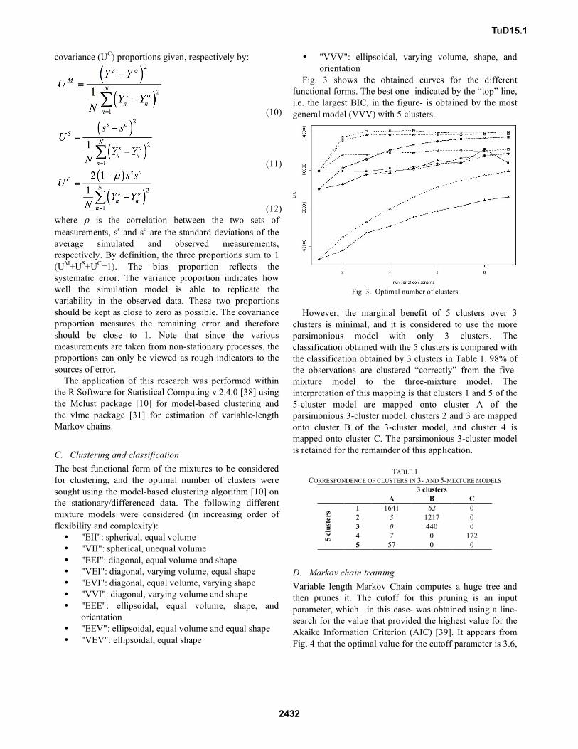
Fig. 3 shows the obtained curves for the different

functional forms. The best one -indicated by the “top” line,

i.e. the largest BIC, in the figure- is obtained by the most

general model (VVV) with 5 clusters.

Fig. 3. Optimal number of clusters

However, the marginal benefit of 5 clusters over 3

clusters is minimal, and it is considered to use the more

parsimonious model with only 3 clusters. The

classification obtained with the 5 clusters is compared with

the classification obtained by 3 clusters in Table 1. 98% of

the observations are clustered “correctly” from the five-

mixture model to the three-mixture model. The

interpretation of this mapping is that clusters 1 and 5 of the

5-cluster model are mapped onto cluster A of the

parsimonious 3-cluster model, clusters 2 and 3 are mapped

onto cluster B of the 3-cluster model, and cluster 4 is

mapped onto cluster C. The parsimonious 3-cluster model

is retained for the remainder of this application.

TABLE 1

CORRESPONDENCE OF CLUSTERS IN 3- AND 5-MIXTURE MODELS

3 clusters

A B C

1 1641 62 0

2 3 1217 0

3 0 440 0

4 7 0 172

5 c

lust

ers

5 57 0 0

D. Markov chain training

Variable length Markov Chain computes a huge tree and

then prunes it. The cutoff for this pruning is an input

parameter, which –in this case- was obtained using a line-

search for the value that provided the highest value for the

Akaike Information Criterion (AIC) [39]. It appears from

Fig. 4 that the optimal value for the cutoff parameter is 3.6,

TuD15.1

2432

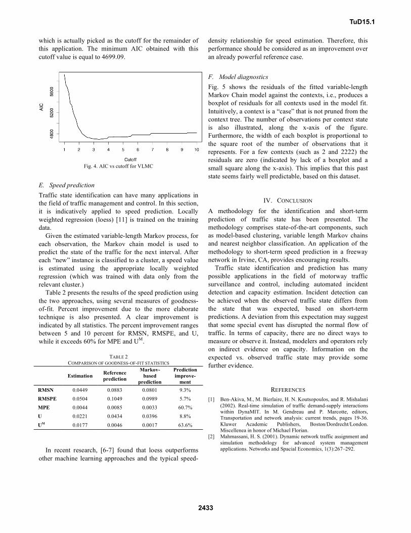
which is actually picked as the cutoff for the remainder of

this application. The minimum AIC obtained with this

cutoff value is equal to 4699.09.

Fig. 4. AIC vs cutoff for VLMC

E. Speed prediction

Traffic state identification can have many applications in

the field of traffic management and control. In this section,

it is indicatively applied to speed prediction. Locally

weighted regression (loess) [11] is trained on the training

data.

Given the estimated variable-length Markov process, for

each observation, the Markov chain model is used to

predict the state of the traffic for the next interval. After

each “new” instance is classified to a cluster, a speed value

is estimated using the appropriate locally weighted

regression (which was trained with data only from the

relevant cluster.)

Table 2 presents the results of the speed prediction using

the two approaches, using several measures of goodness-

of-fit. Percent improvement due to the more elaborate

technique is also presented. A clear improvement is

indicated by all statistics. The percent improvement ranges

between 5 and 10 percent for RMSN, RMSPE, and U,

while it exceeds 60% for MPE and UM

.

TABLE 2

COMPARISON OF GOODNESS-OF-FIT STATISTICS

Estimation Reference

prediction

Markov-

based

prediction

Prediction

improve-

ment

RMSN 0.0449 0.0883 0.0801 9.3%

RMSPE 0.0504 0.1049 0.0989 5.7%

MPE 0.0044 0.0085 0.0033 60.7%

U 0.0221 0.0434 0.0396 8.8%

UM 0.0177 0.0046 0.0017 63.6%

In recent research, [6-7] found that loess outperforms

other machine learning approaches and the typical speed-

density relationship for speed estimation. Therefore, this

performance should be considered as an improvement over

an already powerful reference case.

F. Model diagnostics

Fig. 5 shows the residuals of the fitted variable-length

Markov Chain model against the contexts, i.e., produces a

boxplot of residuals for all contexts used in the model fit.

Intuitively, a context is a “case” that is not pruned from the

context tree. The number of observations per context state

is also illustrated, along the x-axis of the figure.

Furthermore, the width of each boxplot is proportional to

the square root of the number of observations that it

represents. For a few contexts (such as 2 and 2222) the

residuals are zero (indicated by lack of a boxplot and a

small square along the x-axis). This implies that this past

state seems fairly well predictable, based on this dataset.

IV. CONCLUSION

A methodology for the identification and short-term

prediction of traffic state has been presented. The

methodology comprises state-of-the-art components, such

as model-based clustering, variable length Markov chains

and nearest neighbor classification. An application of the

methodology to short-term speed prediction in a freeway

network in Irvine, CA, provides encouraging results.

Traffic state identification and prediction has many

possible applications in the field of motorway traffic

surveillance and control, including automated incident

detection and capacity estimation. Incident detection can

be achieved when the observed traffic state differs from

the state that was expected, based on short-term

predictions. A deviation from this expectation may suggest

that some special event has disrupted the normal flow of

traffic. In terms of capacity, there are no direct ways to

measure or observe it. Instead, modelers and operators rely

on indirect evidence on capacity. Information on the

expected vs. observed traffic state may provide some

further evidence.

REFERENCES

[1] Ben-Akiva, M., M. Bierlaire, H. N. Koutsopoulos, and R. Mishalani

(2002). Real-time simulation of traffic demand-supply interactions

within DynaMIT. In M. Gendreau and P. Marcotte, editors,

Transportation and network analysis: current trends, pages 19-36.

Kluwer Academic Publishers, Boston/Dordrecht/London.

Miscellenea in honor of Michael Florian.

[2] Mahmassani, H. S. (2001). Dynamic network traffic assignment and

simulation methodology for advanced system management

applications. Networks and Spacial Economics, 1(3):267–292.

TuD15.1

2433

Fig. 5. Residuals vs. Context plot for vlmc

[3] Wang, Y., M. Papageorgiou, and A. Messmer. A Real-Time

Freeway Network Traffic Surveillance Tool. IEEE Transactions on

Control Systems Technology, vol. 14, 2006, pp. 18-32.

[4] Einbeck, J., Tutz, G. (2004). Modelling beyond Regression

Functions: an Application of Multimodal Regression to Speed-Flow

Data. SFB Discussion Paper 395.

[5] Sun, L. and J. Zhou. Developing Multi-Regime Speed-Density

Relationships Using Cluster Analysis. Transportation Research

Record: Journal of the Transportation Research Board 1934, D.C.,

2005, pp. 64–71.

[6] C. Antoniou and H. N. Koutsopoulos. Estimation of Traffic

Dynamics Models with Machine Learning Methods. Accepted for

publication in Transportation Research Record 1965, pp. 103-111,

Washington D.C., 2006.

[7] C. Antoniou and H. N. Koutsopoulos. A Comparison of Machine

Learning Methods for Speed Estimation. Proceedings of the 11th

IFAC Symposium on Control in Transportation Systems, Delft, The

Netherlands, August 29-31, 2006.

[8] Bock, H. H. (1998a), “Probabilistic Approaches in Cluster

Analysis,” Bulletin of the International Statistical Institute, 57, 603–

606.

[9] Bock, H. H. (1998b), “Probabilistic Aspects in Classification,” in

Data Science, Classification and Related Methods, eds. C. Hayashi,

K. Yajima, H. H. Bock, N. Oshumi, Y. Tanaka, and Y. Baba,

NewYork:Springer-Verlag, pp. 3–21.

[10] C. Fraley and A. E. Raftery (2002), Model-Based Clustering,

Discriminant Analysis, and Density Estimation. Journal of the

American Statistical Association, Vol. 97, No. 458, pp. 611-631.

[11] Mitchell, T. M. Machine Learning. WCB McGraw Hill, 1997.

[12] Wolfe, J. H. (1970), “Pattern Clustering by Multivariate Mixture

Analysis,” Multivariate Behavioral Research, 5, 329–350.

[13] Edwards, A. W. F., and Cavalli-Sforza, L. L. (1965), “A Method for

Cluster Analysis,” Biometrics, 21, 362–375.

[14] Day, N. E. (1969), “Estimating the Components of a Mixture of

Normal Distributions,” Biometrika, 56, 463–474.

[15] Scott, A. J., and Symons, M. J. (1971), “Clustering Methods Based

on Likelihood Ratio Criteria,” Biometrics, 27, 387–397.

[16] Duda, R. O., and Hart, P. E. (1973), Pattern Classification and

Scene Analysis, New York: Wiley.

[17] Binder, D. A. (1978), “Bayesian Cluster Analysis,” Biometrika, 65,

31–38.

[18] McLachlan, G. J., and Basford, K. E. (1988). Mixture Models:

Inference and Applications to Clustering, New York: Marcel

Dekker.

[19] Banfield, J. D., and Raftery, A. E. (1993), “Model-Based Gaussian

and Non-Gaussian Clustering,” Biometrics, 49, 803–821.

[20] Cheeseman, P., and Stutz, J. (1995), “Bayesian Classification

(AutoClass): Theory and Results,” in Advances in Knowledge

Discovery and Data Mining, eds. U. Fayyad, G. Piatesky-Shapiro,

P. Smyth, and R. Uthurusamy, AAAI Press, pp. 153–180.

[21] Fraley, C., and Raftery, A. E. (1998), “How Many clusters? Which

Clustering Method? Answers via Model-Based Cluster Analysis,”

The Computer Journal, 41, 578–588.

[22] Friedman, H. P., and Rubin, J. (1967), “On Some Invariant Criteria

for Grouping Data,” Journal of the American Statistical Association,

62, 1159–1178.

[23] Murtagh, F., and Raftery, A. E. (1984), “Fitting Straight Lines to

Point Patterns,” Pattern Recognition, 17, 479–483.

[24] Schwarz, G., 1978. "Estimating the dimension of a model". Annals

of Statistics 6(2):461-464.

[25] Markov, A.A. "Extension of the limit theorems of probability theory

to a sum of variables connected in a chain". reprinted in Appendix B

TuD15.1

2434

of: R. Howard. Dynamic Probabilistic Systems, volume 1: Markov

Chains. John Wiley and Sons, 1971.

[26] Geroliminis N., Skabardonis A., 2005, “Prediction of arrival

profiles and queue lengths along signalized arterials using a Markov

decision process” Transportation Research Record, 1934, 116-124

[27] Abaza, K. A., S. A. Ashur, and I. A. Al-Khatib. Integrated

Pavement Management System with a Markovian Prediction Model.

Journal of Transportation Engineering, Vol. 130, No. 1, pp. 24-33,

January 1, 2004.

[28] Scherer, W. T., and D. M. Glagola. Markovian models for bridge

maintenance management. Journal of Transportation Engineering,

Vol. 120, No. 1, pp. 37-51, January/February, 1994.

[29] Ortiz-Garcia, J. J. , S. B. Costello, and M. S. Snaith. Derivation of

Transition Probability Matrices for Pavement Deterioration

Modeling. Journal of Transportation Engineering, Vol. 132, No. 2,

pp. 141-161, February 1, 2006.

[30] Stamoulakatos, T. S., and E. D. Sykas (2006). Hidden Markov

modeling and macroscopic traffic filtering supporting location-

based services. Wireless communications and mobile computing (in

press).

[31] Maechler M. and Buehlmann P. (2004) Variable Length Markov

Chains: Methodology, Computing, and Software. Journal of

Computational and Graphical Statistics 2, 435-455.

[32] Rissanen, J. (1983), ‘A universal data compression system’, IEEE

Trans. Inform. Theory IT-29, 656–664.

[33] Toledo T., and H.N. Koutsopoulos (2004), Statistical Validation of

Traffic Simulation Models, Transportation Research Record 1876,

pp 142-150.

[34] Ashok, K. and Ben-Akiva, M. (2000). Alternative approaches for

real-time estimation and prediction of time-dependent origin–

destination flows. Transportation Science, 34(1):21–36.

[35] Ashok, K. and Ben-Akiva, M. (2002). Estimation and prediction of

time-dependent origin-destination flows with a stochastic mapping

to path flows and link flows. Transportation Science, 36(2):184–

198.

[36] Pindyck R.S. and Rubinfeld D.L. (1997). Econometric Models and

Economic Forecasts, 4th Edition. Irwin McGraw-Hill, Boston MA.

[37] Theil, H. (1961). Economic Forecasts and Policy. North-Holland,

Amsterdam, The Netherlands.

[38] R Development Core Team (2006). R: A language and environment

for statistical computing. R Foundation for Statistical Computing,

Vienna, Austria, 2006, http://www.R-project.org (accessed

November 23, 2006).

[39] Akaike, H. (1974). "A new look at the statistical model

identification". IEEE Transactions on Automatic Control 19 (6):

716–723.

TuD15.1

2435