constrained curves and surfaces proposal · 2015-03-12 · tive industry, robotics, numerically...

Constrained Curves and surfaces Proposal

Sebti Foufou, Lionel Garnier, Dominique Michelucci

December 2009

Chapter 1

The big picture

Our project will enable the emergence of a generation of Qatarian researchersin the essential field of computerized geometry.

The goal is to apply the geometric constraints approach, up to now usedfor dimensionning and tolerancing parts in CAD-CAM, to curves and surfacesmodeling.

Geometric modelling is today essential for numerous applications: automo-tive industry, robotics, numerically controled machining, control of industrialproduction through artificiel vision, computer aided surgery, virtual reality, sim-ulations, video games, image synthesis.

Geometric constraints are today used routinely by all geometric modellers inthe market for dimensioning and tolerancing industrial parts. Designers specifygeometric constraints on a geometric sketch : angle or distance between geomet-ric elements (points, lines, planes, cercles, spheres), or incidences (coplanarities,collinearities) and tangency relations between geometric elements. These con-straints are translated into a system of equations, which is solved, for eaxmple,with some Newton-Raphson iterations from the initial guess provided by thesketch. The modeller also performs a qualitative study of the system of con-straints, either with some graph-based method which counts degrees of freedom,or with a witness-based method. This qualitative study planifies the numericalsolving of the system. In a nutshell, this qualitative study detects under-, well-,and over-constrained subsystems, and it also reduces well-constrained parts intoirreducible well-constrained subsystems, which speeds up the resolution process.Today, geometic constraints is sufficiently mature, and all professional geometricmodellers provides a solver of geometric constraints.

D. Michelucci, a member of this project, is an expert of geometric modellingwith constraints. He has co-chaired GCR 2006 to GCR 2010 (GCR: GeometricConstraints and Reasoning). He was guest co-editor of a special issue in IJCGAon this topic. He is a guest co-editor of a special issue in CGTA after GCR2009. He authors several articles in this topic.

Our project aims a high level modelling of curves and surfaces for CAD-CAM (Computer-Aided Design, Computer-Aided Manufacturing), relying on

3

4 CHAPTER 1. THE BIG PICTURE

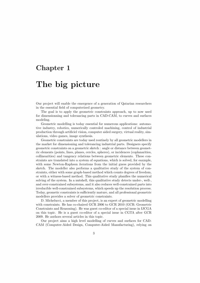
methods in Geometric Constraints: this field is still in its infancy. A surveyabout constrained curves and surfaces is [1] (D. Menegaux, one of the authorsof [1], was PhD student of D. Michelucci). The followig pictures are extractedfrom this article [1].

Our goal: We would like that designers and engineers specify a set of ge-ometric or topologic properties which shapes must fulfil, starting from somesketch of the shape. This sketch can be for example a low-resolution triangularor quadrangular mesh. Users can interactively edit the sketch, it ie moving somevertices. Features lines are then either automatically extracted (dihedral anglesare filtered with some angular threshold), or users interactively draw them onthe sketch. Feature lines are visually and geometrically relevant because the sur-face is only C0-continuous along features lines. Then the modeller computes thedegrees of the algebraic or rational triangular and quadrilateral patches, for thesurface to have the specified level of continuity (C1=G1, or C2, or G2), as in [2].Several kinds of surfaces will be considered, from polynomial or rational Bzierpatches, to NURBS, through Steiner patches or some kinds of Dupin cyclides(Lionel Garnier is an expert of Dupin cyclides). A numerical solver is then usedto compute a witness (an example of solution), and to detect remaining degreesof freedom, with a numerical study of the jacobian of the system of equations atthe witness. These degrees of freedom enable users to interactively modify theshape: for instance, some control points or some normal vectors can be inter-actively modified by the user (in passing, some haptic devices and interface canbe convenient), and the modeller updates the shape. Usually, some Newton-Raphson iterations should be sufficient, but it is also possible to use a moregeneral solver, at some singularity : it may happen that a continuous modifica-tion of the value of some parameter needs to ”jump” on another solution. Thisgeneral solver is anyway needed to solve global constraints, such as minimizingthe curvature gradients of the surface or other beautyfying constraints.

The witness method is presented in several articles [3, 4, 5, 6, 7, 8], and usedin industrial CAD-CAM solvers, e.g. CATIA. As far as we are aware of, it isnot used for modeling constrained curves and surfaces up to now.

The scientific background of the numerical solver is presented in §2. It is

5

also presented in recent articles [9, 10, 11, 12], some still unpublished. Mainly,we aim to optimize this solver, to program it on GPU, to extend it (for tran-scendental equations for example), and to use it for modeling constrained curvesand surfaces.

A commented bibliography on surface modelling, in general and in the Di-jon’s team, is presented in §3.

6 CHAPTER 1. THE BIG PICTURE

Chapter 2

GPU Bernstein Solvers forBig Systems

2.1 Introduction

This text summarizes the scientific background of the solver for the QATARproposal [9, 10, 11, 12].

Geometric Constraints Solving is today essential for all geometric modellersused in CAD-CAM and in Computer Graphics. Tensorial Bernstein bases areused in several solvers, by Garloff and Smith [13], by Mourrain and Pavone [14],by Michelucci and Foufou [10], and many others, especially in the CAD-CAMfields and Computer Graphics where Bernstein-Bezier curves and surfaces areroutinely used. But polynomials become exponential size in this base, makingsuch solvers impracticable for systems with more than 6 or 7 unknowns. Re-cently, D. Michelucci [15] showed that resorting to linear programming solvesthis difficulty: Bernstein based solvers can be used with big systems. Moreover,the solver can straightforwardly manage inequalities, and it can be extended tonon algebraic systems involving transcendentals exp, cos, sin, arccos, etc. Thegoal of this project is to implement on GPU such a solver.

For the moment, there are two CPU implementations of the new solver. Thefirst program is due to Michelucci [15]; it is written in Ocaml and uses eitherfloating point arithmetic, or exact rational arithmetic; it is a constructive proofof feasability for this kind of solver; it has detected the sticking points of thesolver, like inaccuracy. The floating point arithmetic variant fails due to inac-curacy; the exact arithmetic variant never fails but is terribly slow. The secondprogram is due to Christoph Fuenfzig [12] during his post doctoral sojorn inDijon, in Michelucci’s team; it is written in C++, it uses floating point arith-metic and the SoPlex software for solving LP problems. Christoph’s programis numerically very reliable (we know no failure due to inaccuracy), though ithas not been formally proved yet. Both programs are sequential and run onCPU. Articles related to the solver are [15, 10, 9, 12, 11]. For conciseness, this

7

8 CHAPTER 2. GPU BERNSTEIN SOLVERS FOR BIG SYSTEMS

text skips several related issues: detecting over- or under-constrained systemsand decomposing well-constrained systems into irreducible systems [7, 6, 5], andtranslating geometric constraints into equations.

2.1.1 The context

Today all geometric modellers in the market provide modelling with geometricconstraints. Typically, designers provide a sketch with some interactive tools,called a sketcher, and specify geometric constraints which must be fulfiled: align-ments or coplanarities of points, distances betwen points or between points andlines or planes, angles between lines or planes, tangency or incidence relations,etc. A numerical solver then interactively corrects the sketch in order to sat-isfy the specified constraints. The first solvers already used the coordinates ofthe sketch interactively provided by the designer to feed some Newton-Raphsonalgorithm. This approach is sometimes unsufficient: for instance, the Newton-Raphson iterations may not converge or converge to a root which is not the oneexpected by the designer; this unexpected behavior sometimes persists whenthe Newton-Raphson method is replaced with an homotopy (also called contin-uation) [16].

It also happens that the designer needs to know all real roots, or wantsa guarantee that a system has no real root at all, or that the system has aunique root. For instance, when designing a new kind of robot, roboticians mayneed to prove that an articulated robot is safe and can not self intersect, orthat modifying its driving parameters (e.g. the lengths of its jacks) will yieldto only one possible configuration of the robot, i.e. the robot can not meeta bifurcation point or any other singularity for a given command curve in theparameters space of the robot.

To summarize, some applications need to compute all roots of systems ofequations. Interval solvers, for instance Newton interval solvers, Bernstein basedsolvers, or other geometric solvers like the solver by Kim and Elber [17] (it relieson another geometric bases, the rational spline functions) on one hand, and onthe other hand homotopy solvers, are able to find all real (or complex) rootsof systems of equations. However, all these solvers have limitations: homotopysolvers are restricted to polynomial systems; interval Newton solvers are slow,especially for big systems, because of the well known wrapping effect of intervalanalysis; using the tensorial Bernstein bases (or other geometric bases like themultivariate rational spline functions bases) cancels the wrapping effect; unfor-tunately, polynomials which are sparse in the canonical tensorial base becomedense and thus exponential size in the tensorial Bernstein base; the consequenceis that current Bernstein based solvers, or Elber and Kim’s solver becomes un-usable for systems with more than 6 or 7 unknowns and equations. Anotherrestriction of current tensorial Bernstein based solvers is that they apply only topolynomial systems. Simplicial (also called projective) Bernstein based solvers(suggested in [4], implemented in [18]) avoid both the wrapping effect and theexponential overhead of the tensorial Bernstein bases: the simplicial Bernsteinbases have polynomial size. However, simplicial Bernstein based solvers have

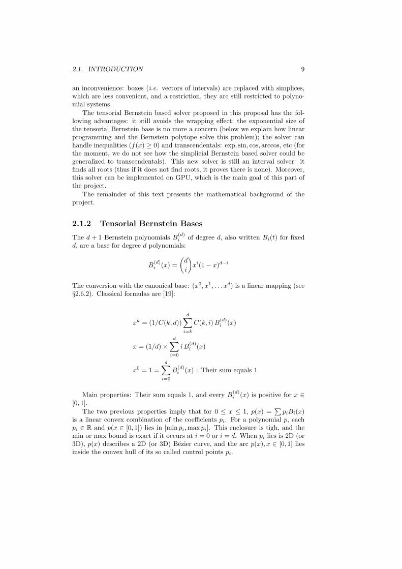
2.1. INTRODUCTION 9

an inconvenience: boxes (i.e. vectors of intervals) are replaced with simplices,which are less convenient, and a restriction, they are still restricted to polyno-mial systems.

The tensorial Bernstein based solver proposed in this proposal has the fol-lowing advantages: it still avoids the wrapping effect; the exponential size ofthe tensorial Bernstein base is no more a concern (below we explain how linearprogramming and the Bernstein polytope solve this problem); the solver canhandle inequalities (f(x) ≥ 0) and transcendentals: exp, sin, cos, arccos, etc (forthe moment, we do not see how the simplicial Bernstein based solver could begeneralized to transcendentals). This new solver is still an interval solver: itfinds all roots (thus if it does not find roots, it proves there is none). Moreover,this solver can be implemented on GPU, which is the main goal of this part ofthe project.

The remainder of this text presents the mathematical background of theproject.

2.1.2 Tensorial Bernstein Bases

The d + 1 Bernstein polynomials B(d)i of degree d, also written Bi(t) for fixed

d, are a base for degree d polynomials:

B(d)i (x) =

(d

i

)xi(1− x)d−i

The conversion with the canonical base: (x0, x1, . . . xd) is a linear mapping (see§2.6.2). Classical formulas are [19]:

xk = (1/C(k, d))d∑

i=k

C(k, i) B(d)i (x)

x = (1/d)×d∑

i=0

i B(d)i (x)

x0 = 1 =d∑

i=0

B(d)i (x) : Their sum equals 1

Main properties: Their sum equals 1, and every B(d)i (x) is positive for x ∈

[0, 1].The two previous properties imply that for 0 ≤ x ≤ 1, p(x) =

∑piBi(x)

is a linear convex combination of the coefficients pi. For a polynomial p, eachpi ∈ R and p(x ∈ [0, 1]) lies in [min pi,max pi]. This enclosure is tigh, and themin or max bound is exact if it occurs at i = 0 or i = d. When pi lies is 2D (or3D), p(x) describes a 2D (or 3D) Bezier curve, and the arc p(x), x ∈ [0, 1] liesinside the convex hull of its so called control points pi.


0 1

B0 ≥ 0

B1 ≥ 0

B2 ≥ 0

4y+x−3 = 0

3/5 7/90 1

B0 ≥ 0

B1 ≥ 0

B2 ≥ 0

Figure 2.1: Left: The Bernstein polytope encloses the curve: (x, y = x2), for(x, y) ∈ [0, 1]2. Its limiting sides are: B0(x) = (1 − x)2 = y − 2x + 1 ≥ 0,B1(x) = 2x(1 − x) = 2x − 2y ≥ 0, B2(x) = x2 = y ≥ 0. Right: Solving4x2+x−3 = 0, with x ∈ [0, 1], is equivalent to intersecting the line 4y+x−3 = 0with the curve (x, x2). Linear programming gives the intersection between theline and the Bernstein polytope.

Example: since x = 0 B0(x) + 1/dB1(x) + 2/dB2(x) + . . . d/d Bd(x), thepolynomial curve (x, y = p(x)), with x ∈ [0, 1], lies in the convex hull of itscontrol points (i/d, pi).

Contrarily to coefficients in the usual base: (1, x, x2, . . . xd), control pointsdepend on the x interval. The classical de Casteljau method provides the controlpoints of p(x), x ∈ [0, t], and of p(x), x ∈ [t, 1] (actually, t can be outside theinterval [0, 1], but the numerical stability is lost).

For multivariate polynomials, the TBB is the tensorial product:

(B(d1)0 (x1), . . . B

(d1)d1

(x1))× (B(d2)0 (x2), . . . B

(d2)d2

(x2))× . . .

The convex hull properties and the de Casteljau method extend to the TBB,which provide sharp enclosure of multivariate polynomials p(x), x ∈ [0, 1]n.

Garloff and Mourrain’s solvers express multivariate polynomials in the TBB:they first convert polynomials from the canonical base to the TBB, then they usethe multivariate de Casteljau algorithm. The new solver we want to implementon GPU does not need to express multivariate polynomials in the TBB.

2.1.3 The limitation of current Bernstein based solvers

Computer Graphics and CAD-CAM, and more recently numerical analysis useproperties of TBB for computing covers (Fig. 2.9) or intersection points betweenBezier curves and surfaces, for enclosing multivariate polynomials or Bezier

2.1. INTRODUCTION 11

y

x

z

y

z

x

Figure 2.2: The Bernstein polytope enclosing the surface patch: (x, y, z = xy).Inequalities of delimiting planes are: Bi(x)Bj(y) ≥ 0, where i = 0, 1 and B0(t) =1− t and B1(t) = t.

(1, 1, 1)

(0, 0, 0)

(1/3,0,0) (2/3, 1/3, 0)

Figure 2.3: The Bernstein polytope, a tetrahedron, enclosing the curve (x, y =x2, z = x3) with x ∈ [0, 1]. Its vertices are v0 = (0, 0, 0), v1 = (1/3, 0, 0),v2 = (2/3, 1/3, 0) and v3 = (1, 1, 1). v0 lies on B1 = B2 = B3 = 0, v1 onB0 = B2 = B3 = 0, etc. B0(x) = (1 − x)3 = 1 − 3x + 3x2 − x3 ≥ 0 ⇒1−3x+3y−z ≥ 0, B1(x) = 3x(1−x)2 = 3x−6x2+3x3 ≥ 0 ⇒ 3x−6y+3z ≥ 0,B2(x) = 3x2(1− x) = 3x2 − 3x3 ≥ 0 ⇒ 3y − 3z ≥ 0, B3(x) = x3 ≥ 0 ⇒ 3z ≥ 0.


curves and surfaces, and for solving systems of algebraic equations [13, 14, 17,18, 20]. We will not detail these solvers, for the sake of conciseness, but theyall express the multivariate polynomials in the TBB, (except [18] which usesimplicial Bernstein bases), since they require tight enclosures of polynomials.Unfortunately, the TBB has exponential cardinality (1+d1)× (1+d2) . . .× (1+dn), where di is the max degree of unknown xi. Even for linear systems, thesize is exponential: 2n. Admittedly, the canonical base has also exponential size,but systems are sparse in the canonical base, and they are no more in the TBB.Here is a striking illustration: in the TBB, the monomial 1 has exponential size,it is written 1 = (B(d1)

1 (x1)+ . . . B(d1)d1

(x1))× . . . (B(dn)1 (xn)+ . . . B

(dn)dn

(xn)). Inother words, all basis functions of the TBB are needed to express the constantpolynomial 1, and all coefficients equal the real number 1.

Clearly, existing Bernstein based solvers become impracticable for n > 6 orn > 7. Much bigger algebraic systems arise in Geometric Constraints Solving,especially in 3D. For instance, the 20 vertices of a regular (or non regular) dodec-ahedron can be specified with the lengths of its 30 edges, and the coplanaritiesof its 12 faces; this problem does not seem to be reducible.

There are two ways to overcome this limitation of current Bernstein basedsolvers: first, using the simplicial Bernstein base instead of the TBB; the sim-plicial base has polynomial cardinality [4, 18], it replaces boxes with simplices.Second, the solution proposed in this proposal: it is the first polynomial timemethod to overcome the exponential size of the TBB. It remarks that onlythe smallest and the greatest coefficients in the TBB are interesting, becausethey bound the polynomial. The main idea is to consider a polytope (a con-vex polyhedron) which we call the Bernstein polytope; this polytope can bedefined either as the convex hull of its vertices, or as the intersection of the halfspaces of its hyperplanes. Classical TBB solvers use the first definition: eachvertex of the corresponding polytope (which could be called the TBB polytope,or the TBB simplex) corresponds to a coefficient of a polynomial expressed inthe TBB; these solvers are trapped with the exponential number of vertices,and the exponential number of hyperplanes of the TBB polytope. The methodproposed here uses the second definition for the Bernstein polytope, the num-ber of bounding hyperplanes of which is polynomial: for instance for quadraticsystems in n unknowns (i.e. every monomial has total degree 2 or less), thereare O(n2) hyperplanes, and O(3n) vertices. Intuitively, the exponential numberof vertices is a necessary condition for computing tight ranges.

Fuenfzig et al define and compare four Bernstein related polytopes [9].

2.2 The new solver

2.2.1 Bernstein polytopes

For univariate polynomials, the inequalities: Bi(x) ≥ 0 are used to define thehyperplanes of faces of a convex polyhedron, which we call the Bernstein poly-tope, and which encloses the curve in Rd: (xi = xi), with x ∈ [0, 1]. For d = 2,

2.2. THE NEW SOLVER 13

the Bernstein polytope is a triangle, see Fig. 2.1 and counting multiplicities,each triangle side meets the curve in 2 points. For d = 3, the Bernstein polytopeis a tetrahedron, see Fig. 2.3, and counting multiplicities, each plane meets thecurve in 3 points. The extension to higher degrees is straightforward but 2D or3D representations are no more possible.

The Bernstein polytope also extends to multivariate polynomials. Fig. 2.2shows the 3D Bernstein polytope, a tetrahedron, which encloses the surfacepatch (x1, x2, x1x2), or, to use more usual and intuitive notations: (x, y, z = xy).The hyperplanes are here planes in 3D space, they are:

B(1)0 (x)×B

(1)0 (y) ≥ 0 ⇒ (1− x)(1− y) ≥ 0

⇒ 1− x− y + z ≥ 0

B(1)0 (x)×B

(1)1 (y) ≥ 0 ⇒ (1− x)y ≥ 0

⇒ y − z ≥ 0

B(1)1 (x)×B

(1)0 (y) ≥ 0 ⇒ x(1− y) ≥ 0

⇒ x− z ≥ 0B

(1)1 (x)×B

(1)1 (y) ≥ 0 ⇒ xy ≥ 0

⇒ z ≥ 0

This tetrahedron is optimal because it is the convex hull of the patch.More generally, the inequalities for multivariate polynomials are obtained as

the product of the inequalities for univariate polynomials. Actually, up to thebinomial coefficient factor, it is also true for the inequalities in the univariatecase: they are products (B(1)

0 (x))d−i × (B(1)1 (x))i = (1− x)d−ixi.

A paper submitted to publication [9] defines and compares four Bernsteinrelated polytopes, and empirically shows that the previously defined Bernsteinpolytope is the best tradeoff: it has polynomial complexity (a polynomial num-ber of delimiting hyperplanes, and an exponential number of vertices), and itprovides ranges which are almost as tight as the ones obtained when using theTBB (when it is possible to use the TBB and to compare, of course). TheBernstein polytope which gives the same ranges as the TBB, and which couldbe called the TBB polytope or simplex, has an exponential number of verticesand an equal number of hyperplanes; it has thus an intrinsically exponentialcomplexity, which makes it non-practicable for more than 6 or 7 unknowns.

2.2.2 Resorting to Linear Programming

This section first shows on a simple example how the Bernstein polytope reducesthe computation of an enclosure of a polynomial, and the reduction of a domainpreserving roots, to linear programming (LP) problems [21, 22]. The latter aresolved with the classical simplex method in two stages: the first stage computesa feasable point if any, or detects the feasable set is empty; the second stage findsthe vertex of the polytope which optimizes a given linear objective function. Itis known that this method is not polynomial time in the worst case, but it iscompetitive in practice with polynomial time methods.


0 1

4y +x−3 = 2

4y +x−3 = 0

4y +x−3 = −3

4y +x−3 = −5/2

B0 ≥ 0

B1 ≥ 0

B2 ≥ 0

Figure 2.4: Bounding 4x2 + x− 3, 0 ≤ x ≤ 1.

2.2.3 Bounding: 4x2 + x− 3, 0 ≤ x ≤ 1

To compute a lower and an upper bound of the polynomial p(x) = 4x2 + x− 3,for x ∈ [0, 1], minimize, and maximize, the linear objective function: 4y + x− 3on the Bernstein polytope (the triangle in Fig. 2.1) enclosing the curve (x, y =x2), x ∈ [0, 1]. It is a LP problem, after replacing x2 with y:

min p = 4y + x− 3, max p = 4y + x− 3B0 = y − 2x + 1B1 = −2y + 2xB2 = yx ≥ 0, y ≥ 0, B0 ≥ 0, B1 ≥ 0, B2 ≥ 0

Notations are self explanatory. See Fig. 2.4. The simplex algorithm [21, 22]provides the enclosure [−3, 2] (which is optimal, since the min −3 occurs at


vertex x = 0, and the maximum 2 occurs at vertex x = 1):

min p = −3 + x + 4yB0 = 1− 2x + yB1 = 2x− 2yB2 = y

max p = 2− 5B0 − 9/2B1

x = 1−B0 −B1/2y = 1−B0 −B1

B2 = 1−B0 −B1

Remember that variables on the right side (”not in base”) have values 0. Onlythe max part is commented1. In max p = 2 − 5B0 − 9/2B1, the value of pcan not be greater than 2: variables on the right side B0 and B1 are zero,and increasing one of them or both will only decrease p due to the negativecoefficients −5B0 − 9/2B1 in the objective function.

Consistently: at vertex v0 = (0, 0) where B1 = B2 = 0, the polynomial valueis p0 = p(0) = −3; at vertex v1 = (1/2, 0) where B0 = B2 = 0, the polynomialvalue is p1 = p(1/2) = −3/2; at vertex v2 = (1, 1) where B0 = B1 = 0, thepolynomial value is p2 = p(1) = 2. These values p0, p1, p2 are the coefficientsin the Bernstein base, or control points, of p(x): p(x) = p0B0(x) + p1B1(x) +p2B2(x). This property extends to all univariate and multivariate polynomials.It is a consequence of the definition of Bernstein polytopes.

Using other inequalities (we use: B(2)1 (x) ≤ 1/2) often provides tigher

bounds. This is not compatible with the standard approach of TBB [14, 10, 17].

2.2.4 Solving: 4x2 + x− 3 = 0, x ∈ [0, 1]

This section shows how the solver reduces intervals or boxes containing roots,for the simple equation 4x2 + x − 3 = 0 for x ∈ [0, 1]. Solving is equivalent tofinding the intersection points between the line 4y + x − 3 = 0, and the curve(x, y = x2). This curve is enclosed in its Bernstein polytope: the triangle of Fig.2.1. Intersecting the line and the triangle, i.e. finding the min and max valueof x, will reduce the interval for x; it is the same LP problem as above, exceptwe minimize and maximize x. Solutions are:

min x = 3/5 + 2/5B1

x = 3/5 + 2/5B1

y = 3/5− 1/10B1

B0 = 2/5− 9/10B1

B2 = 3/5− 1/10B1

max x = 7/9− 4/9B0

x = 7/9− 4/9B0

y = 5/9 + 1/9B0

B1 = 4/9− 10/9B0

B2 = 5/9 + 1/9B0

Thus the interval [0, 1] for x has been reduced to [3/5, 7/9]. To furtherreduce this interval, apply a scaling (§2.2.7) to map x ∈ [3/5, 7/9] to X ∈ [0, 1]:x = 3/5 + (7/9 − 3/5)X = b + aX, and the equation in X is: 4a2X2 + (8ab +b)X +(b− 3) = 0. LP is used again to reduce the interval. Convergence arounda regular root is very fast, but is not discussed for conciseness, and anyway

1This tableau form is used only for presentation. Today the revised simplex form is pre-ferred. It is also possible to use an interior point method to solve the linear programmingproblems.


Mourrain et al already studied the complexity, the convergence rate and thesize of the stack [14]. We can re-use their results because ranges provided bythe Bernstein polytope are almost as tight as the ones given by the min and themax of the TBB coefficients.

Remarks: if the line does not cut the Bernstein polytope, then the LP prob-lem is not feasable and the interval [0, 1] contains no roots.

2.2.5 Box reduction

For simplicity, we assume that the system is quadratic, i.e. all monomials haveat most degree 2. It is without loss of generality, since all algebraic systems canbe rewritten as quadratic systems, with the addition of a polynomial number ofauxilliary unknowns and equations, using iterated squaring: for instance, x4 isreplaced with x2

2, where x2 is a new variable, and with an auxilliary equationx2 − x2 = 0.

The Bernstein polytope of a quadratic system with n unknowns has 3n

vertices, but only O(n2/2) hyperplanes. They are B(2)i (xk) ≥ 0 for i ∈ 0, 1, 2

and k ∈ [1, n], and B(1)i (xk)B(1)

j (xl) ≥ 0 for all i ∈ 0, 1, j ∈ 0, 1, k ∈ [1, n − 1],l ∈ [k + 1, n]. It is worth to also use: 1/2−B1(xk) ≥ 0.

A variable of a LP problem is attached to each of the m monomials: xk tomonomial xk, xkl to monomial xkxl (k < l), xkk to x2

k.Assume roots are searched in [0, 1]n: it is without loss of generality (§2.2.7).

Then each quadratic equation in the system gives a linear constraint in theLP problem. Each quadratic inequality in the system gives a linear inequalityconstraint in the LP problem.

To reduce the box [0, 1]n, preserving roots, 2n LP problems are solved: min-imize and maximize xk for k ∈ [1, n]. If the corresponding LP problem is notfeasable, then the box contains no root.

2.2.6 Higher degrees

Higher degrees reduce to quadratic using auxilliary unknowns and equations. Itis also possible to extend the definition of the Bernstein polytope to arbitrarydegrees. For total degree d, and for n unknowns x1, . . . xn, the Bernstein poly-tope has O((d + 1)n) vertices and O(nd) hyperplanes. For sparse polynomials,the number of useful hyperplanes can be decreased. Finding the best way tomanage higher degrees is one of the task of this proposal.

2.2.7 Scaling

After reduction, the reduced box is no more [0, 1]n. A scaling maps the box[u, v], where ui ≤ vi, to the unit hypercube [0, 1]n: define xi = ui + (vi− ui)Xi,wi = vi−ui, X ∈ [0, 1]n. Then x2

i = w2i X2

i +2uiwiXi +u2i , xixj = wiwjXiXj +

uiwjXj + ujwiXi + uiuj .Scaling is a linear mapping in the space of the LP variables: Xi, Xii, Xij .


Another approach scales the Bernstein polytope, leaving unchanged equa-tions and inequalities of the system. For a box xi = [ui, vi] with wi, the hyper-planes of the Bernstein polytope are changed as follows (as usual, the monomialx2

i is represented with the variable xii in the LP problems, and the monomialxixj with the variable xij).

B(2)0 (xi) = (1− xi)2 ≥ 0 becomes:

(vi − xi)2 = x2i − 2vixi + v2

i = xii − 2vixi + v2i ≥ 0

B(2)1 (xi) = 2xi(1− xi) ≥ 0 becomes:

2(xi − ui)(vi − xi) = 2(−xii + (ui + vi)xi − uivi) ≥ 0

B(2)2 (xi) = x2

i ≥ 0 becomes:

(xi − ui)2 = xii − 2uixi + u2i ≥ 0

B(1)0 (xi)B

(1)0 (xj) = (1− xi)(1− xj) ≥ 0 becomes:

(vi − xi)(vj − xj) = xij − vixj − vjxi + vivj ≥ 0

B(1)0 (xi)B

(1)1 (xj) = (1− xi)xj ≥ 0 becomes:

(vi − xi)(xj − uj) = −xij + ujxi + vixj − viuj ≥ 0

B(1)1 (xi)B

(1)1 (xj) = xixj ≥ 0 becomes:

(xi − ui)(xj − uj) = xij − ujxi − uixj + uiuj ≥ 0

It straightforwardly extends to higher degrees.Christoph Fuenfzig et al used the latter scaling method [12]. Michelucci used

the former one [15].

2.2.8 Description of the new solver

The solver manages as usual a stack of boxes to be studied. This stack isinitialized with the domain where roots are searched. While the stack is notempty, the top box is popped and studied.

First the box is reduced. If the LP problem is not feasable, this box containsno root. If the reduced box is small enough (or if some Newton-Kantorovitchtest guarantees that it contains a unique regular root), the box is inserted in alist of roots; possibly, the root is polished with some standard Newton-Raphsoniterations, starting from the center of the box). It the box is not small enoughbut it is significantly reduced, then another reduction is performed; otherwisethe box is bisected along its longest side (or along the side which has been lessreduced) and the two halves are pushed on stack. Possibly, a list of residualboxes is also managed: they are small boxes where the method can not conclude:for instance they contain very close regular roots or singular roots.


Some optimizations: The previous call to the simplex method often gives afeasable point, thus the first stage of the simplex method can often be avoided.The quadratic system can be sparse, which can reduce the number of monomialsand LP variables xkl, xkk, as well as the number of relevant hyperplanes: e.g.inequalities involving xkl are useless if the monomial xkxl is unused. Finally,when reducing a box along xl, it is possible to use the already reduced intervalsfor xk, k < l. Note however that this last optimization is possible only for aCPU program, and becomes impossible when the reductions are performed inparallel on GPU.

Several variants are possible; see [12] for a comparison of some variants witha CPU (sequential) implementation.

2.2.9 Advantages of the new solver

This solver has many advantages. It solves in polynomial time the difficultywhich blocks previous TBB solvers.

It is easy to account for other inequalities (§2.2.10), in order to reduce thevolume of the Bernstein polytope.

There is no need for inversing the jacobian of the system, or for precondi-tioning: LP does all the work. Actually, the fact that preconditioning does nothelp can be seen as a limitation: there is no easy way to improve the new solver!

Also previous TBB solvers need a special treatment to detect as soon aspossible boxes without roots. For example, in 2D, consider 2 very close and”parallel” curves. Without this special treatment, when searching for intersec-tion points of the two curves, the previous TBB solvers have to subdivide spaceall along the two curves, in order to separate them, which is time consuming.This kind of configuration extends in any dimension. For instance, the solverin [10] searches with linear programming if there is a linear combination of thecontrol points which is everywhere strictly positive (actually greater or equal to1): if such a linear combination exists, then the box contains no root. Mourrainet al use two other methods. An advantage of the new solver is that it detectsthese problematic configurations without any special treatment: again, linearprogramming does all the job. Again, this feature means that there is no easyway to improve the new solver.

Basically, the new solver applies to under-, to well- and to over-constrainedsystems. Over-constrained systems have not been tested up to now; this projectwill be an opportunity for.

Almost all bisections are useful, i.e. they separate roots.The convergence is quadratic around a regular root. The rate of convergence,

and the size of the stack are studied in Mourrain et al [14].The extension to higher degrees than quadratic is straightforward but can

be done in several ways, which will have to be compared during the project.The method can manage transcendentals: exp, cos, arccos: it is sufficient

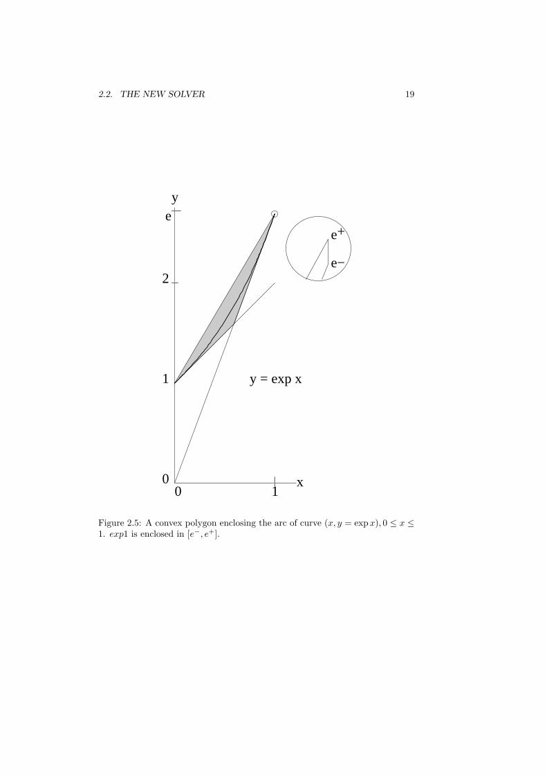
to enclose the curves (x, expx), (x, cos x), etc inside a convex polygon: see Fig.2.5. It is one task of this proposal. This feature is an important advantage,when compared to other methods like homotopy.


+

0

1

2

e

0 1

y

x

y = exp x

e

e−

Figure 2.5: A convex polygon enclosing the arc of curve (x, y = exp x), 0 ≤ x ≤1. exp1 is enclosed in [e−, e+].


Finally, this method is mathematically simple: a lot of students in Com-puter Science can program it on CPU. The only burden is the management ofinaccuracy, see §2.3.2.

2.2.10 Chebychev and minimax variant

A foreruner is Olivier Beaumont: he uses Chebychev polynomials and LPfor enclosing multivariate polynomials in his PhD, in 2002, at Ecole NormaleSuperieure de Lyon, France (in French). It is possible to use Chebychev poly-topes instead of Bernstein polytopes, or to use both (i.e. to use both inequal-ities). In the univariate case, Chebychev inequalities are obtained as follows:the monomial xd is interpolated at the d Gauss points with a degree d− 1 poly-nomial T (x); then the error is bounded with [b0, b1], which gives inequalitiesb0 ≤ xd − T (x) ≤ b1. Actually, any approximation scheme, using its own inter-polation points, will give inequalities e.g. the minimax polynomial. Inequalitiesin the multivariate case (x1, x2 . . . xn) are again given by products of univariateinequalities.

A difficulty with Chebychev polytopes (as they are implicitly defined byBeaumont) is that both their number of vertices and hyperplanes are exponentialwith the dimension. We have not studied yet if a variant with polynomialcomplexity is possible.

2.2.11 An interval Newton variant

To help intuition and understanding, this paragraph proposes a variant of thenew solver which is closer to interval Newton solvers (in §2.6.1). Assume thequadratic system F (x) = 0 is well constrained, and J is the inversible jacobianof F at the center of the studied box B. Compute coefficients of all momomialsof all polynomials of N(x) = x − F (x)J−1, i.e. the Newton map (there areO(n3) coefficients, it is the size of F ); an approximate inverse is sufficient;actually all classical optimizations can be used, such as a LUP decompositionof J . Asymptotically, around a regular root r, N(x) is eventually close tox − r + O((x − r)2). Bound the n polynomials of N(x ∈ B) with the methodin §2.2.3; it provides a box B′. All roots in B are in B′. So, if B ∩ B′ isempty, it is guaranteed that B contains no root. If B ∩B′ is sufficiently small,or some Newton-Kantorovitch test guarantees that B ∩ B′ contains a uniquesingular root, add this box (or its center) to a list of solutions. If the box is notsmall enough, but has been significantly reduced, apply another reduction step(J and J−1 may be updated or not, according to the variant). If the box hasnot been significantly reduced, bisect it and pushes the two halves on the stackof boxes to be studied. Remark that contrarily to the new solver, this variantneeds numerical linear algebra (LUP decomposition, or matrice inverses). Also,this latter variant can not handle systems with inequalities as nicely as the newsolver (§2.2).

2.3. IMPLEMENTATIONS ISSUES 21

2.3 Implementations issues

2.3.1 GPU implementations

This solver offers 3 possibilities for parallelism: first, in the simplex method,pivoting can be done in parallel on all rows; russian students reported a speed-up factor 7 with a GPU implementation. Second, reducing a box in Rn requiressolving 2n independent LP problems. Third, each box in the stack of boxes tobe studied can be treated independently.

Both existing implementations, Michelucci’s [15] and Fuenfzig’s [12] areCPU, i.e. sequential. The goal of this project is to produce GPU implementa-tions of the solver. A challenge is to output dozens, or hundreds, or thousandsof roots in real time. Empirically, with circle packing problems [12], the methodon CPU is O(n3.5) time A GPU implementation should divide by a factor n(if the 2n LP problems for reducing a box are performed in parallel) or more,due to an intrinsic parallelism in the simplex method (or in the interior pointmethod).

2.3.2 Inaccuracy issue

The Bernstein polytope encloses very tighly the underlying algebraic manifold:

(x1, . . . xn, x21, . . . x

2n, x1x2, . . . xn−1xn), xi ∈ [0, 1]

thus with a naive floating point implementation, some roots are missed becauseof rounding errors. For instance, when solving x2 − x = 0 with x ∈ [0, 1], theline y − x = 0 is considered (see Fig. 2.1); if this line becomes y − x = ε withε > 0 due to inaccuracy, the two roots are missed.

Rational arithmetic

The conceptually simplest solution resorts to exact computations with rationalnumbers. We did it, and roots are no more missed (reassuring!), but the program(on CPU) becomes 100 or 1000 times slower, and unusable. Several optimiza-tions can be considered. First, do not waste digits: round boxes outwards aftereach reduction, e.g. prefer the box [2, 3] to the box [20001/10000, 29999/10000];it has been implemented. Second, use the lazy paradigm: first perform oper-ations with interval arithmetics (intervals bounds are floating point numbers,and outwards rounding is used), and resort to exact rational arithmetic onlywhen it is unavoidable. We did not test the latter: anyway, rational arithmeticwould likely be one order of magnitude slower than the next approach, and italso prevents handling transcendentals (cos, arccos, exp, π, . . .) which is plannedin this proposal. Also, GPU does no provide rational arithmetic, nor dynamicallocation and garbage collection, up to now.


Figure 2.6: Left: each bounding line of a 2D convex are sandwiched betweentwo parallel lines (which are not exactly parallel to the exact sandwiched line).Right: superposition of the exact polygon and its outer aproximation. Thethickness of the sandwich is exagerated.

Interval Linear Programming

The second solution to the numerical inaccuracy is to use some kind of intervalLP.

Our solution is directed by two ideas: intervals are thin, typically some ULPslarge, because they are used only to contain rounding errors. Second, we mustbe conservative: when computing the max value for an unknown xk, we can becontent with an upper bound of the exact result; we can also accept that, whenthe exact feasible set is empty, the computed feasible set is not (though thesmaller the better, of course): thus no root is missed. For short, the solution isonly presented with an example: since all unknowns lie in [0, 1], the line Ax +By+C = 0 where A,B, C are (thin) intervals, and which is obtained after somepivoting, is replaced with the thick line: ax+by+(A−a+B−b+C) = 0, where aand b are floating point midpoints of A and B, and the interval A−a+B−b+Cis computed with interval arithmetic: it is the only interval occuring in this row.Geometrically, it means that the feasible set is enclosed in a convex polytope,which slowly grows during each pivoting step of the simplex method, see Fig.2.6. Algebraically, after each pivoting operation, the inaccuracy of coefficientsin each row is collected and stored in the column of the constants; thus onlyone column of the LP simplex contains intervals. Actually, since all hyperplanesare pushed outwards, only the upper bound of the interval is relevant, and nointerval need to be stored. The modifications to the classical simplex methodin two stages are thus easy.

This method is self validating: it detects when the studied box is too small for

2.4. TOPICS AND TASKS 23

the accuracy provided by the floating-point arithmetic; in this case, the thicknessof hyperplanes corresponding to equations of the system is no more negligible infront of the size of the box (the unit hypercube). Eventually bisections becomeuseless; to give an intuitive account, imagine that intervals have integer bounds;then the left and right halves of the interval [0, 1] are [0, 1] itself. The same kindof things occurs with floating point bounds, due to the discreteness of floatingpoint numbers.

Wilkinson’s analysis

Christoph Fuenfzig et al implement a third solution, using the condition numberof an underlying matrice and an analysis due to Wilkinson [12].

Tolerances

§2.3.2 presents a method to manage small inaccuracies. To manage bigger inac-curacies, such as tolerances used in CAD-CAM, the cleanest approach is to useinequalities instead of equations: the solution set is no more made of isolatedpoints (or curves, surfaces in case of an under-constrained system), but it is aregion of Rn with non zero n-volume. The solver proposed here can at leastin principle be adapted to output an inner and an outer representation of thesolution set: inner boxes lie completely inside the solution set, and outer boxescover the solution set. The Haussdorf distance between the inner and the outerrepresentation should be prescribed. The isotopy of the boundaries of the innerand the outer representations is is an interesting topic for a future research veryrelevant for CAD-CAM, but it is not part of this proposal.

2.4 Topics and tasks

This section lists some tasks and topics of this proposal. This list is indicative;it may be amended.

- CPU implementations. Elaborating from the existing solvers, we planto realize, test and compare some CPU implementations of a solver of quadraticsystems, handling inaccuracy and interval linear programming. Several variantscan be tried and compared, e.g. scaling can be managed in 2 ways. A criteriumof choice can be the compatibility with the argument reductions used for dealingwith transcendentals functions.

- GPU implementations. The main goal of the project is to realize GPUimplementations of a solver of quadratic systems, handling inaccuracy and in-terval linear programming. Several variants can be tried and compared. Forexample, is it interesting to use a Newton-Kantorovitch test, to detect as soonas possible when the classical Newton iteration is contracting in a box, and willconverge to its unique root? Is it possible to adapt this test to the features ofthe Bernstein polytope?

- Optimizations. We mention one of the possible optimizations not testedso far, and we wish to investigate. The dual LP problem has the same size and


32 2 2

0

1

Figure 2.7: The dual method traverses dual vertices 1, 2, 3. It traverses nestedbounding boxes. It can shrink the (filled) Bernstein polytope at each iteration,i.e. more often than the primal method.

complexity as the primal LP problem. The dual method traverses dual verticeswhich are not vertices of the feasible polytope (except the last one, which is thesearched optimum) but are optimal. For a maximization LP problem, currentdual vertices in the dual method always give an upper bound of the maximum,and this upper bound decreases at each iteration, until the exact maximum ofthe LP problem is reached. Symmetrically for a minimization problem. Thusduring the reduction process of a bounding box for the roots x = (x1, . . . xn),the dual method traverses a decreasing set of nested bounding boxes. Now, theBernstein polytope enclosing the quadratic patch inside a given box for x is afunction of this enclosing x box, so it can be updated, actually shrinked, at eachiteration of the dual method. The idea is illustrated Fig. 2.7. This optimizationis not possible with the primal method, or more precisely the primal methodmust wait to reach the optimum before it can shrink the Bernstein polytope.

- Geometric constraint solving. Another task is to test the solver forGeometric Constraint Solving problems. Dassault Systemes has a database ofnearly two thousand examples of geometric constraints solving. It is also possibleto automatically build circle packing problems with any size (see Appendix§2.6.5); these systems are quadratic and have a unique solution.

- Higher degrees. They can be dealt with in several ways: for instance theycan be reduced to quadratic systems adding auxilliary unknowns and equations,or the Bernstein polytope can be extended to higher degrees. The project willimplement both on CPU or GPU, and compare.

- proving a system has no real root at all. The solver presented herecan prove that a box contains no root, but it is not sufficient for proving thatthere is no root at all. Several methods can be considered for compactifyingthe problem (geometric inversion, homogenization [23], etc). We will try andcompare these methods.

- Transcendentals. We plan CPU and GPU implementations of transcen-dentals: the latter may occur in Geometric Constraint Solving, and the solvercan handle them. Computer Arithmetic uses argument reductions, e.g. thecomputation for a given number θ of cos θ is reduced to the computation of

2.4. TOPICS AND TASKS 25

cos 2θ or of cos θ/2. These methods have to be adapted to cope with the factthat the argument θ is no more a given number, but a given interval.

- Special equations. We hope to be able to dealing with special equations.For instance, some polynomial equations are not given as a sum of monomials,but as the nullity of the determinant of a square k × k matrice M ; this occursfor Cayley-Menger determinants and their variants [24]. These determinantsprovide coordinate-free equations. The polynomial expansion of the determinantof a k × k matrice is O(k!) size, or worse when the entries in the matrice arepolynomials. A polynomial space solution is to introduce k new variables λi,and k new equations:

∑i λiMij = 0, for j = 1, . . . k, to express the linear

dependence between the rows of the matrice M , and an equation∑

i λ2i = 1.

More generally, one of the task of the project is to facilitate the translation ofconstraints into equations acceptable by the new solver.

- Decomposition. This text assumed for simplicity that the system arewell-constrained, i.e. that they have a finite number of solutions. One of thetasks is to study the case of under- and over-constrained systems in more details.More generally, one task in the project is to interface the solver with existingsoftwares which decompose systems of constraints into sub-systems, and diag-nose errors in systems of geometric constraints. Such softwares are alreadyavailable in the Dassault Systemes solver. Under-constrainedness has severalcauses. First, it is well known that rigid systems of geometric constraints areintrinsically under-constrained: for instance in 2D a triangle, represented withthe 6 coordinates of its vertices, is completely described with 3 constraints (forinstance 2 angles and one length), thus it remains 3 degrees of freedom for pin-ning the triangle in the plane; this under-constrainedness can be solved adding 3auxilliary equations in 2D, and 6 in 3D. Another cause of under-constrainednesscan be due to the interactive protocol: constraints are incrementally inserted.A last cause can be due to the fact that the designer describes a whole curve orsurface (e.g. the unit circle is described with x2 + y2− 1 = 0 in 2D), and wantsto use the solver to compute a cover of the curve or surface, as in Fig. 2.9.Concerning over-constrainedness, it is either structural (too much equations in-volve a subset of unknowns; this case is easy to detect), or due to some nontrivial geometric theorem: detecting the latter dependences is a hard problem,except if a witness is known [7, 6, 5]. Fortunately, the new solver works evenin presence of dependent equations. It can also be used to compute a witness[7, 6, 5].

- Theoretical complexity. Actually, the size of the stack and the rate ofconvergence should be equal to the ones for the Mourrain’s solver [14]. Fuenfziget al empirically found that the solver runs in O(n3.5) time for solving circlepacking problems [12].

- Other extensions. For instance, Elber and Kim’s solver relies on the basisof rational spline function. This geometric basis has properties very similar tothe ones of the Bernstein basis. Spline functions are piecewise algebraic orrational functions. Is is possible to define a related spline polytope? Also, isit possible to extend the solver to account for subdivision surfaces (which aretoday fashionable in Computer Graphics, and percolate to CAD-CAM) and IFS


fractals?- Cycling. Some simplex programs cycle in presence of geometric degenera-

cies. Bland’s pivoting rule avoids cycling, but the classical proof does not takeinaccuracy into account. We envision to work on Coq or Gappa proofs of theinterval simplex method.

- Dealing wih tolerances (§2.3.2) It is a more distant goal. It is not partof this proposal. Once the new solver will be available, it will be possible totackle other questions: computing the topology of a set defined by a system,computing one point on each connected component of this set, computing if itis simply connected or not, etc , in the spirit and wake of Delanoue, Jaulin andCottenceau [25].

2.5 Conclusion

This text has presented the scientific background concerning the solver for theQATAR proposal: it is the first solver which overcomes in polynomial time thedifficulty due to the exponential cardinality of the tensorial Bernstein base: themain idea is to define a Bernstein polytope not from its vertices (which are inexponential size) but from its hyperplanes (which are in polynomial number).Other tightening inequalities can be used (minimax or Chebychev polynomi-als). The solver can handle inequalities, under-, well- and over-constrainedsystems, and transcendental equations. Difficulties due to inaccuracy can beovercome. We envision GPU implementations, extensions to transcendentals,Coq or Gappa proofs of the interval simplex method.

2.6 Appendix

2.6.1 Interval Newton solvers

Assume the system is f(X) = 0, and it is well-constrained. Interval Newtonsolvers typically manage a stack of boxes to be studied. A box is just a vectorof intervals. While the stack is not empty, a box B is popped. The newtonmap is n(x) = x−J−1f(x), where J is the jacobian at the center Bc of the boxB. n(B) is evaluated with some interval analysis; for instance, centered intervalevaluation uses: g(B) ∈ g(Bc) + (B − Bc)g′(B) to enclose g(B); used with theNewton map, it gives the Krawczyk Moore operator. Possible roots in B all liein n(B). If n(B) ( B, then B contains only one root, and the standard Newtonmap will converge to this root. If B ∩ n(B) is empty, then B contains no root.If B ∩ n(B) is non empty, it contains all roots of B; if B ∩ n(B) is significantlysmaller than B, another reduction step is performed, otherwise B is bisectedalong its longuest side, and the two halves are pushed on stack.

Remark that it makes no sense to evaluate n(B) with naive interval compu-tations: the interval width of a sum (or a difference) is the sum of the intervalwidths of the operands, so the interval n(B) = B± something will never beincluded in B.

2.6. APPENDIX 27

Other interval Newton solvers use interval inverses of the jacobian f ′(B).

2.6.2 Conversion from the canonical and the Bernsteinbase

The Bernstein polynomials are a base for degree d polynomials. The conversionwith the canonical base: (x0, x1, . . . xd) is a linear mapping, e.g. for degree 3:

B0(t)B1(t)B2(t)B3(t)

=

1 −3 3 −10 3 −6 30 0 3 −30 0 0 1

1tt2

t3

1tt2

t3

=

1 1 1 10 1/3 2/3 10 0 1/3 10 0 0 1

B0(t)B1(t)B2(t)B3(t)

Remark: Garloff and Mourrain’s solvers need to express polynomials in thetensorial Bernstein base, and thus to convert the polynomial equations into theTBB. The solver proposed here does not need such a conversion; instead, it usesinequalities: B

(d1)i1

(x1)B(d2)i2

(x2) . . . ≥ 0.

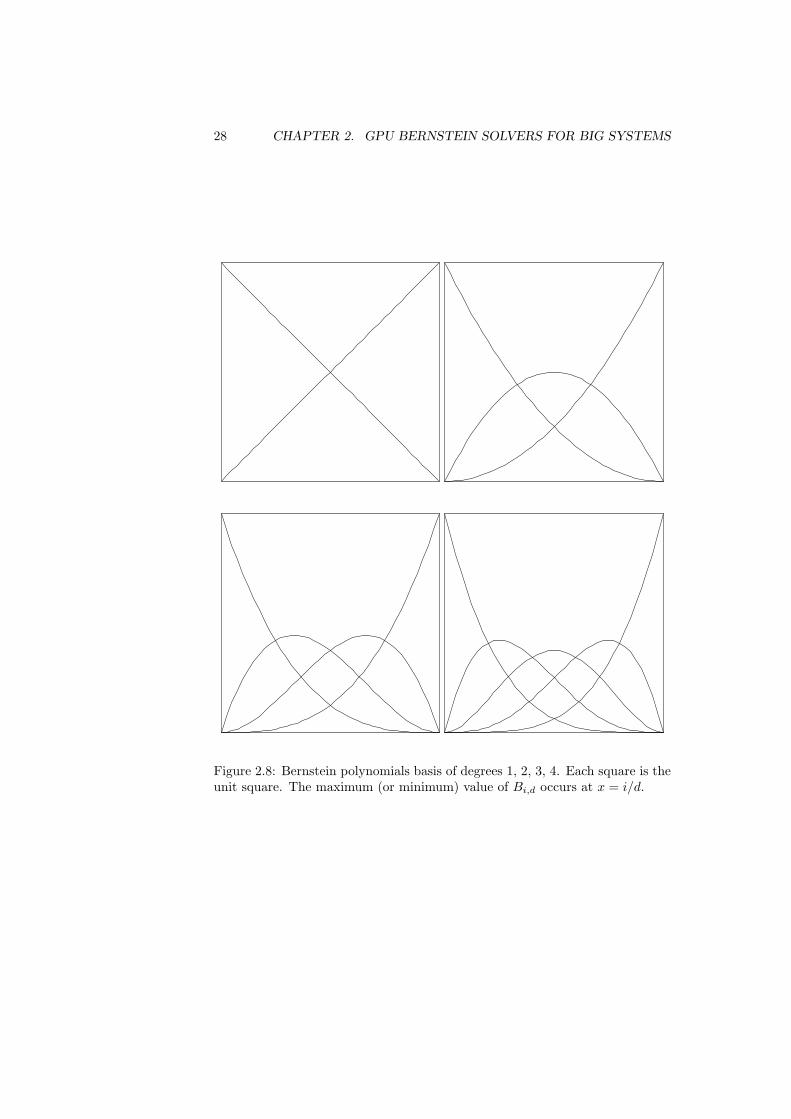
2.6.3 Bernstein polynomials basis

See Fig. 2.8.

2.6.4 TBB avoids the wrapping effect

Fig. 2.9 visually shows that the tensorial Bernstein base gives tigher enclo-sures of polynomials than the naive interval arithmetic. Polytope-based rangemethods are compared in [9].

2.6.5 Circle packing

Circle packing problems are a convenient way to test the new solver [12]. Em-pirically, Fuenfzig’ solver is O(n3.5) time, where n is the number of circles. See[12] for details.

The circle packing problem2 is : given a completely triangular planar graph,represent each vertex with a circle, such that each time two vertices are con-nected by an edge, the two corresponding circles are exteriorly tangent. TheKoebe - Andreev - Thurston theorem states that the solution is basically unique,modulo Mobius transformations and orthogonal symmetries, for instance it isunique if the coordinates of the 3 vertices of the enclosing triangle are given.An algorithm due to K. Stephenson is available on internet, it uses repeatedlocal relaxations. It is possible to generate automatically such problems with

2Search ”Circle packing theorem” on wikipedia.


Figure 2.8: Bernstein polynomials basis of degrees 1, 2, 3, 4. Each square is theunit square. The maximum (or minimum) value of Bi,d occurs at x = i/d.

2.6. APPENDIX 29

Figure 2.9: Four implicit polynomial curves f(x, y) = 0 are plotted with therecursive subdivision method, above using the naive interval arithmetic, belowusing Bernstein bases. The latter needs much less subdivisions for detectingthat a curve does not cross the studied square.

any size: generate n − 3 random 2D points Pi, i = 4, . . . n, inside a triangleP1P2P3, then compute the Delaunay triangulation of the n points Pi: it gives acompletely triangular planar graph. Forget the coordinates. Fix arbitrarily thecoordinates of the 3 vertices of the exterior triangle P1P2P3, and then solve withthe solver the system of equations, which is, for each edge PiPj of the graph:(xi − xj)2 + (yi − yj)2 − (Ri + Rj)2 = 0; the circle for Pi has center (xi, yi) andradius Ri.

In passing, the circle packing problem seems to resist to decomposition meth-ods (e.g. Owen’s method) used in Geometric Constraint Solving.

Chapter 3

Constrained curves andsurfaces: a commentedbibliography

31

32CHAPTER 3. CONSTRAINED CURVES AND SURFACES: A COMMENTED BIBLIOGRAPHY

Bibliography

[1] V. Cheutet, M. Daniel, S. Hahmann, R. L. Greca, J.-C. Leon, R. Mac-ulet, D. Menegaux, and B. Sauvage, “Constraint modeling for curves andsurfaces in cagd: A survey,” International Journal of Shape Modeling, 2007.

[2] M. Boschiroli, C. Fuenfzig, L. Romani, and G. Albrecht, “Etat de l’art desmethodes d’interpolation locale de maillages triangulaires par des facettesnon planes c0-continues state of the art on local c0 continuous interpolationmethods for triangular meshes),” in Journees de l’AFIG, 2009.

[3] S. Foufou, D. Michelucci, and J.-P. Jurzak, “Numerical decomposition ofgeometric constraints,” in ACM Symp. on Solid and Physical Modelling,pp. 143–151, 2005.

[4] D. Michelucci, S. Foufou, L. Lamarque, and P. Schreck, “Geometric con-straints solving: some tracks,” in ACM Symp. on Solid and Physical Mod-elling, pp. 185–196, 2006.

[5] D. Michelucci and S. Foufou, “Geometric constraints solving: the witnessconfiguration method,” Computer Aided Design, vol. 4, no. 38, pp. 284–299,2006.

[6] D. Michelucci and S. Foufou, “Detecting all dependences in systems ofgeometric constraints using the witness method,” in Automatic Deductionin Geometry, ADG 2006, LNAI 4869, pp. 98–112, 2007.

[7] D. Michelucci and S. Foufou, “Interrogating witnesses for geometric con-straint solving,” in SIAM/ACM Joint Conference on Geometric and Phys-ical Modeling, (San Francisco), october 2009.

[8] D. Michelucci, S. Foufou, L. Lamarque, and D. Menegaux, “Anotherparadigm for geometric constraints solving,” in CCCG, 2006.

[9] C. Fuenfzig and D. Michelucci, “Polytope-based computation of polynomialranges,” in submitted to SAC 2010, 2009.

[10] D. Michelucci and S. Foufou, “Bernstein basis for interval analysis: ap-plication to geometric constraints systems solving,” in 8th Conference onReal Numbers and Computers (Bruguera and Daumas, eds.), pp. 37–46,July 2008.

33

34 BIBLIOGRAPHY

[11] C. Fuenfzig and D. Michelucci, “Optimizations for Bernstein-based solversusing domain reduction,” in submitted to TMCE 2010, 2009.

[12] F. C, D. Michelucci, and S. Foufou, “Nonlinear systems solver in floating-point arithmetic using linear programming reduction,” in SIAM/ACMJoint Conference on Geometric and Physical Modeling, (San Francisco),october 2009.

[13] J. Garloff and A. P. Smith, “Investigation of a subdivision based algorithmfor solving systems of polynomial equations,” Journal of nonlinear analysis: Series A Theory and Methods, vol. 47, no. 1, pp. 167–178, 2001.

[14] B. Mourrain and J.-P. Pavone, “Subdivision methods for solving polynomialequations,” Tech. Rep. RR-5658, INRIA, August 2005.

[15] D. Michelucci, “Linear programming for interval Newton solvers,” in Au-tomated Deduction in Geometry, (Shanghai), september 2008.

[16] H. Lamure and D. Michelucci, “Solving geometric constraints by homo-topy,” IEEE Trans on Visualization and Computer Graphics, vol. 2, pp. 28–34, 1996.

[17] G. Elber and M.-S. Kim, “Geometric constraint solver using multivariaterational spline functions,” in SMA’01: Proc. of the 6th ACM Symp. onSolid Modeling and Applications, (New York, NY, USA), pp. 1–10, ACMPress, 2001.

[18] M. Reuter, T. S. Mikkelsen, E. C. Sherbrooke, T. Maekawa, and N. M. Pa-trikalakis, “Solving nonlinear polynomial systems in the barycentric Bern-stein basis,” Vis. Comput., vol. 24, no. 3, pp. 187–200, 2008.

[19] G. Farin, Curves and Surfaces for CAGD: A Practical Guide. AcademicPress Professional, Inc., San Diego, CA, 1988.

[20] E. C. Sherbrooke and N. M. Patrikalakis, “Computation of the solutions ofnonlinear polynomial systems,” Comput. Aided Geom. Des., vol. 10, no. 5,pp. 379–405, 1993.

[21] T. H. Cormen, C. E. Leiserson, R. L. Rivest, and C. Stein, Introduction toalgorithms. Cambridge, MA: MIT Press, second ed., 2001.

[22] W. Press, S. Teukolsky, W. Vetterling, and B. Flannery, Numerical Recipesin C, the Art of Scientific Computing. Cambridge University Press, 1992.

[23] D. Michelucci and S. Foufou, “Interval-based tracing of strange attractors,”Int. J. Comput. Geometry Appl., vol. 16, no. 1, pp. 27–40, 2006.

[24] D. Michelucci and S. Foufou, “Using cayley-menger determinants for ge-ometric constraint solving,” in SM ’04: Proceedings of the ninth ACMsymposium on Solid modeling and applications, (Aire-la-Ville, Switzerland,Switzerland), pp. 285–290, Eurographics Association, 2004.

BIBLIOGRAPHY 35

[25] N. Delanoue, L. Jaulin, and B. Cottenceau, “Guaranteeing the homotopytype of a set defined by nonlinear inequalities,” Reliable Computing, vol. 13,no. 5, pp. 381–398, 2007.

constrained curves and surfaces proposal · 2015-03-12 · tive industry, robotics, numerically...

Documents