Constrained sampling experiments reveal principles ofdetection in natural scenesStephen Sebastiana,b, Jared Abramsa,b, and Wilson S. Geislera,b,1

aCenter for Perceptual Systems, University of Texas at Austin, Austin, TX 78712; and bDepartment of Psychology, University of Texas at Austin, Austin,TX 78712

Edited by Randolph Blake, Vanderbilt University, Nashville, TN, and approved June 2, 2017 (received for review November 27, 2016)

A fundamental everyday visual task is to detect target objectswithin a background scene. Using relatively simple stimuli, visionscience has identified several major factors that affect detectionthresholds, including the luminance of the background, the contrastof the background, the spatial similarity of the background to thetarget, and uncertainty due to random variations in the propertiesof the background and in the amplitude of the target. Here we usean experimental approach based on constrained sampling frommul-tidimensional histograms of natural stimuli, together with a theo-retical analysis based on signal detection theory, to discover howthese factors affect detection in natural scenes. We sorted a largecollection of natural image backgrounds into multidimensionalhistograms, where each bin corresponds to a particular luminance,contrast, and similarity. Detection thresholds were measured for asubset of bins spanning the space, where a natural backgroundwas randomly sampled from a bin on each trial. In low-uncertaintyconditions, both the background bin and the amplitude of thetarget were fixed, and, in high-uncertainty conditions, they variedrandomly on each trial. We found that thresholds increase approxi-mately linearly along all three dimensions and that detection accuracyis unaffected by background bin and target amplitude uncertainty.The results are predicted from first principles by a normalizedmatched-template detector, where the dynamic normalizing gainfactor follows directly from the statistical properties of the naturalbackgrounds. The results provide an explanation for classic laws ofpsychophysics and their underlying neural mechanisms.

natural scene statistics | detection | masking | normalization | Weber’s law

Visual systems are the result of evolution by natural selection,and, as a consequence, their design is strongly constrained by

the properties of natural visual stimuli and by the specific visualtasks performed to survive and reproduce. Thus, to understandthe human visual system, it is critical to characterize natural vi-sual stimuli and performance in natural visual tasks (1, 2).Perhaps the most fundamental visual task is to identify target

objects in the natural backgrounds that surround us. It is knownthat the specific properties of a background can have a stronginfluence on detectability (Fig. 1). For example, the detectabilityof a target pattern with given amplitude decreases with increasesin background luminance (3, 4), background contrast (5–7), andthe similarity of the spatial properties of the background to thoseof the target (8–12). In addition to the direct effects of suchbackground properties, there are other factors that affect de-tection performance. Specifically, under natural conditions, thestrength (amplitude) and location of the target often randomlyvary on every occasion, and the target typically appears against adifferent background scene on every occasion. The uncertaintycreated by the random amplitude and location of the target(“target uncertainty”) and the random variation in the propertiesof the background (“background uncertainty”) are additionalfactors that can reduce detection performance (12–15).What is relatively unknown are (i) how these various factors

individually affect detection accuracy in natural scenes, (ii) howthey combine in affecting detection accuracy in natural scenes,and (iii) how these factors and the underlying neural mechanisms

are related to the statistical properties of natural scenes. Althoughthere have been a number of studies of detection in naturalbackgrounds (16–23), they have not directly addressed thesequestions, and have either tested only a small number of naturalstimuli (16, 17, 19, 20), tested natural stimuli with altered sta-tistical properties (21, 22), or used experimental paradigms notrepresentative of natural detection tasks (16, 18–20, 23). Theselatter studies are not as representative of natural tasks, becauseobservers were allowed to directly compare the same image withand without the added target, an advantage that is not normallyavailable under real-world conditions.Here we address the three questions above using an experi-

mental approach based on sampling from multidimensional his-tograms of natural stimuli, together with a theoretical analysisbased on signal detection theory. This constrained sampling ap-proach is efficient and could be used to address similar questionsfor other natural tasks. The first step is to obtain a large collectionof calibrated natural images. These images then are divided intomillions of background patches that are sorted into narrow binsalong dimensions of interest. In the present study, each histogrambin corresponds to a narrow range of mean luminance, contrast,and similarity of the target to the background patch. Next, de-tection performance for simple targets is measured by samplingfrom a sparse subset of bins spanning the space. In one set ofexperiments, performance is measured one bin at a time (nobackground and amplitude uncertainty), and, in the second set ofexperiments, the bin is randomly selected on each trial (highbackground and amplitude uncertainty). In both sets of experi-ments, the location of the target (if present) is fixed; i.e., we didnot consider location uncertainty (Discussion). The experimentsrevealed lawful effects of luminance, contrast, and similarity ondetection performance, and showed that humans are remarkably

Significance

The visibility of a target object may be affected by the specificproperties of the background scene at and near the target’s lo-cation, and by how uncertain the observer is (from one occasionto the next) about the values of the background and targetproperties. An experimental technique was used to measurehow several background properties, and uncertainty, affect hu-man detection thresholds for target objects in natural scenes. Thethresholds varied in a highly lawful fashion—multidimensionalWeber’s law—that is predicted directly from the statisticalstructure of natural scenes. The results suggest that the neuralgain control mechanisms underlying multidimensional Weber’slaw evolved because they are optimal for detection in naturalscenes under conditions of high uncertainty.

Author contributions: S.S., J.A., and W.S.G. designed research; S.S., J.A., and W.S.G. per-formed research; S.S. and W.S.G. analyzed data; and S.S. and W.S.G. wrote the paper.

The authors declare no conflict of interest.

This article is a PNAS Direct Submission.1To whom correspondence should be addressed. Email: w.geisler@utexas.edu.

This article contains supporting information online at www.pnas.org/lookup/suppl/doi:10.1073/pnas.1619487114/-/DCSupplemental.

www.pnas.org/cgi/doi/10.1073/pnas.1619487114 PNAS | Published online June 26, 2017 | E5731–E5740

PSYC

HOLO

GICALAND

COGNITIVESC

IENCE

SPN

ASPL

US

unaffected by background and amplitude uncertainty. These aspects ofhuman detection performance are predicted quantitatively from firstprinciples by a signal detection analysis of the natural image stimuli.This analysis provides an understanding of the computational princi-ples and evolutionary pressures that underlie the classic laws of visualpsychophysics and their associated neural mechanisms.

ResultsThe two major aims of the present experiments were (i) to de-termine how the local luminance, contrast, and target similarityof natural backgrounds affect the detectability of targets and(ii) to determine how uncertainty about the background propertiesand target amplitude affect detectability.

Natural Background Stimuli. To obtain stimuli for the experiments,we analyzed a large collection of high-resolution gray-scale nat-ural images (Fig. 2A and Methods). The 1,204 images were di-vided up into millions of background patches that were the samesize (0.8° wide) as the targets used in the detection experiments.For each patch, the mean luminance, root-mean-squared (RMS)contrast, and phase-invariant similarity to the target were mea-sured (see Methods for definitions of these measures). Thesevalues were used to sort the patches into 3D histograms. Fig. 2Bshows the histograms for the two targets used in the experiments.(Note that similarity depends on both the target shape and sizeand hence separate histograms were measured for the two tar-gets.) Most of the 1,000 bins in each of these histograms con-tained many hundreds of patches, and all of the patches within abin had nearly the same mean luminance, contrast, and similarity.However, we note that not all image patches fell into a bin, pri-marily because we restricted the contrast to a maximum of 0.32RMS and the mean luminance to 0.55 of the maximum luminancein the image—the maxima for which it is practical to measurethresholds on standard displays, like those in the present experi-

ments (Methods). Fig. 2C shows single background patches (0.8°wide), each randomly sampled from one of 25 bins with the samemean luminance but different RMS contrast and similarity.

Experiment 1: Detection Thresholds with Background Context Present.In the first experiment, detection thresholds were measured in thefovea along each of the three dimensions separately, with theother two held fixed at their median values. Thresholds weremeasured for two different targets (Fig. 2B), one having a singledominant orientation [a windowed 4-cycles-per-degree (cpd) grat-ing] and one with two dominant orientations (a windowed 4-cpdplaid). To obtain the thresholds, psychometric functions weremeasured in a single-interval identification task with feedback(Fig. 2D). On each trial, a background patch was randomly sam-pled without replacement from the bin being tested. The back-ground that was displayed also included a context region 4.3° widesurrounding the target region. The rest of the display contained afixed luminance equal to that of the bin. In experiment 1, both thetarget amplitude and the background bin were “blocked” (i.e.,fixed for all trials of a block). Randomly, on half of the trials, thetarget was added to the background, and the subject reportedwhether the target was present or absent. Thresholds were definedto be the target amplitude giving 69% correct decisions (Methods).(Note that most studies report thresholds in units of contrast.)The average amplitude thresholds for three subjects are shown in

Fig. 3; Fig. 3, Upper is for the grating target, and Fig. 3, Lower is forthe plaid target (results for individual subjects were similar; see Fig.S1). Each plot shows the threshold (solid symbols) as a function of thevalue along a background dimension. For both targets, the thresholdamplitude increased approximately linearly with local mean lumi-nance in natural backgrounds (solid lines), in agreement withthe classic finding of Weber’s law reported for detection inuniform backgrounds (3, 4). Similarly, the threshold amplitude in-creased linearly with background RMS contrast (at contrasts above afew percent), in agreement with the classic finding for detection inwhite noise (7) and more recent findings for targets in 1/f noise (22,24) and in Gaussianized natural backgrounds (22). Finally, amplitudethreshold increases approximately linearly with the similarity of thebackground to the target, a result not previously reported.The primary conclusion from this experiment is that thresholds

increase approximately linearly along each of the cardinal direc-tions for detection in natural backgrounds, with different slopesand intercepts for each dimension and target. In Signal DetectionAnalysis of Detection Under Blocked Conditions, we show that thisentire pattern of results follows directly from a principled signaldetection theory analysis of detection in natural images.

Experiment 2: Detection Thresholds with Background Context Removed.The first experiment measured detection thresholds when thebackgrounds were substantially larger (4.3° wide) than the target(0.8° wide). It is possible that the surrounding region is helpfulbecause it provides information about the properties of the back-ground in the target region. To examine the effect of the sur-rounding region on threshold, we carried out a second experimentwhere the background was windowed to the size of the target. Thisexperiment also provided some of the baseline data for experiment3 that measured the effects of background and target amplitudeuncertainty. For practical reasons (see experiment 3), we fixed theluminance at the median value in both experiments 2 and 3.Fig. 4 plots the detection thresholds as a function of contrast

and similarity (individual subject data are in Fig. S2). For compar-ison, the contrast and similarity thresholds from experiment 1 alsoare plotted, in a lighter shade. For both targets, threshold stillincreased linearly with the background contrast and similarity.However, the overall magnitude of the thresholds was lower.One possibility is that the decrease is due to reduced uncertaintyabout the location of the target (25, 26). However, between tri-als, a fixation point was kept at the center of the target location,

Fig. 1. Demonstration of the major dimensions of masking. In each case, thesame target (a windowed sinewave grating) is added to the backgrounds on theleft and the right. The target is less visible on the left. (Top) backgrounds areuniform with higher luminance on the left. (Middle) The backgrounds are 2DGaussian noise with higher contrast on the left; mean luminance is the same onboth sides. (Bottom) Backgrounds are 1D Gaussian noise with a horizontal ori-entation on the left; contrast and mean luminance are the same on both sides.

E5732 | www.pnas.org/cgi/doi/10.1073/pnas.1619487114 Sebastian et al.

and, as will be shown in Signal Detection Analysis of DetectionUnder Blocked Conditions, the differences between experiments1 and 2 are predicted by a simple model observer with no posi-tion uncertainty. Thus, it is likely that the primary effect of re-moving the surrounding context region was to remove some ofthe background’s power from under the target.In experiment 3, we consider conditions where the background

bin and target amplitude randomly varied from trial to trial.First, however, we consider potential explanations for the resultsfrom the blocked conditions (experiments 1 and 2) based on thestatistical properties of natural backgrounds.

Signal Detection Analysis of Detection Under Blocked Conditions. Anobvious question is why thresholds should vary approximately

linearly along all three dimensions. To gain some insight into thisfact, we evaluated a simple signal detection model known as amatched-template (MT) observer (Fig. 5A). On each trial, theMT observer computes the dot product of a template f ðx, yÞ withthe input image Iðx, yÞ,

R= f · I =X

x, yf ðx, yÞIðx, yÞ, [1]

where the template is the target (with amplitude equal to 1.0)divided by its energy (the energy of the target is the dot productof the target with itself). Note that the dot product is equivalentto computing the response of a receptive field exactly matchingthe luminance profile of the target. Also note that this template

0

2.9.e3

1.7e5

Similarity

tsartnoC

4.3°

100 ms

400 ms

250 ms

Time

0.8°

C

D

A

B

Fig. 2. Stimuli for experiment 1. (A) Example 400 × 400 pixel regions from several of the 4,284 × 2,844 full images. (B) Three-dimensional histograms alongthe dimensions of luminance, RMS contrast, and similarity, for the two targets used in the experiments: a windowed 4-cpd grating and a windowed 4-cpdplaid. The similarity depends on the specific target, and, hence, there are two histograms (Methods). For each histogram, there are 10 bins along each di-mension (bin widths increase geometrically along each dimension), for a total of 1,000 bins. The ranges for each dimension were restricted to those overwhich it was possible to measure detection thresholds on a standard display screen without clipping (luminance is 0.08 to 0.55 of image maximum, contrast =0.05 to 0.32 RMS, similarity range for grating target is 0.15 to 0.45, and similarity range for plaid target is 0.24–0.47). The color scale indicates the number ofpatches falling in the bins. (C) Example 101 pixel diameter (0.8°) background patches having the same mean luminance and various contrasts and similaritiesto the grating target. (D) Timeline of a single trial (excluding the response and feedback intervals). The psychometric function for each tested bin was basedon at least 350 trials. In the entire experiment, no background patch was presented twice.

Sebastian et al. PNAS | Published online June 26, 2017 | E5733

PSYC

HOLO

GICALAND

COGNITIVESC

IENCE

SPN

ASPL

US

response is sensitive to the phase of the input, whereas thesimilarity measure (which is also based on the shape of thetarget) is insensitive to phase. If the template response R exceedsa decision criterion value γ, then the observer reports that thetarget is present; otherwise, the observer reports that it is absent.The MT observer is the optimal (ideal) observer when the targetis known (as it is here) and the background is Gaussian whitenoise (7, 27, 28), and for “narrow band” targets, it often is nottoo far from optimal if the background is Poisson white noise or iscorrelated Gaussian noise. Although natural image backgroundshave a more complex statistical structure, the MT observer(although not optimal) is a simple, principled signal detectionmodel, and hence a good starting point.The purple histograms in Fig. 5B show the distributions of

template responses for the grating target, for all of the backgroundpatches in three of the 1,000 bins in Fig. 2B. If a target of am-plitude a is added to the background, then the distribution remainsidentical in shape, but is shifted to the right by a (green histo-grams). The distributions are approximately Gaussian, as indi-cated by the curves, which are Gaussian distributions having thesame means and SDs as the measured distributions. We find thatthe distributions of template responses are approximately Gaussianfor almost all of the bins (Fig. S3; see also ref. 29).If the goal of the observer is to be as accurate as possible in

our experiments, where the target is present on half of the trials,then the decision criterion should be placed halfway between thetwo distributions (γ = a=2). In Fig. 5B, the target amplitudes havebeen set so that the accuracy of the MT observer is 85% correctfor the three example bins. In our experiments, we define theamplitude threshold at to be the amplitude producing 69% correctresponses (d′= at=σ = 1.0). In this case, the MT observer’s thresh-old is simply the SD of the template responses for that bin,

at = σðL,C, SÞ, [2]

where L, C, and S represent the luminance, contrast, and similarity,respectively.The symbols in Fig. 6 show the measured SDs of the template

responses, and hence the MT observer’s thresholds, for bothtargets, for all 2,000 bins. To summarize these image statistics,

we fit the following formula, which is separable in luminance,contrast, and similarity:

σðL,C, SÞ= k0ðL+ kLÞðC+ kCÞðS+ kSÞ, [3]

where k0, kL, kC, and kS are free parameters (values in Fig. 6legend). The lines in Fig. 6 show that this formula fits very well(it accounts for 99.6% of the variance in the SDs), implying that

Background Similarity0.25 0.28 0.32 0.37 0.43

Background Contrast0.06 0.12 0.17 0.29

0.16 0.20 0.25 0.31 0.380.06 0.12 0.17 0.29

Background Luminance

Thr

esho

ld A

mpl

itude

0.00

0.08

0.02

0.04

0.06

0.00

0.08

0.02

0.04

0.06

0.09 0.23 0.34 0.50

L = 0.23 L = 0.23

L = 0.23 L = 0.23C = 0.12

C = 0.12

C = 0.12

C = 0.12

S = 0.32 S = 0.32

S = 0.25S = 0.25

HumanMT Obs.

HumanMT Obs.

0.09 0.23 0.34 0.50

Fig. 3. Experiment 1 results: threshold as a function of background luminance, RMS contrast, and similarity to the target, for (Upper) grating and (Lower)plaid targets. Thresholds are for the conditions where the background context region is present (Fig. 2D). Colored symbols are the mean thresholds for threesubjects. Error bars are bootstrapped SDs. The lines are best-fitting linear functions. The black symbols are the predictions of the MT and NMT observer with asingle efficiency scale factor (Eq. 4) applied across all thresholds in experiments 1 and 2 (see also Fig. 4): η= 0.124.

0.06 0.12 0.17 0.29

Thr

esho

ld A

mpl

itude

Background SimilarityBackground Contrast

0.00

0.02

0.04

0.06

0.25 0.28 0.32 0.37 0.43

L = 0.23C = 0.12

L = 0.23S = 0.32

0.06 0.12 0.17 0.29

L = 0.23C = 0.12

0.08

0.00

0.02

0.04

0.06

0.08L = 0.23S = 0.25

0.16 0.20 0.25 0.31 0.38

HumanMT Obs.

Human

MT Obs.

Fig. 4. Experiment 2 results: threshold as a function of RMS contrast and sim-ilarity to the target, for grating and plaid targets, with the background contextregion removed. The colored symbols are themean thresholds for three subjects.Error bars are bootstrapped SDs. The lines are best-fitting linear functions. Theblack symbols are the predictions of the MT and NMT observer with a singleefficiency scale factor (Eq. 4) applied across all thresholds in experiments 1 and 2:η= 0.124. For comparison, the lighter shaded symbols and lines are replottedfrom Fig. 3, where the background context region is present.

E5734 | www.pnas.org/cgi/doi/10.1073/pnas.1619487114 Sebastian et al.

the thresholds of the MT observer are essentially linear in allthree dimensions—multidimensional Weber’s law.The prediction of linear threshold functions for each dimension

is an important result, but do the MT observer’s thresholds ac-tually predict the variation in slopes and intercepts across thedifferent background dimensions and targets in experiments 1 and2 (shown in Figs. 3 and 4)? To address this question, we first notethat, for detection in noise, humans never reach the absolute levelsof performance of the MT (ideal) observer, and thus the relative

performance of human and ideal observers is often compared byintroducing an overall efficiency parameter η, which effectivelyscales up the variance of the MT responses or, equivalently, scalesup all of the MT observer’s thresholds by a constant (7, 12, 28, 30),

at = σðL,C, SÞ� ffiffiffiη

p. [4]

The black symbols in Figs. 3 and 4 show the predictions of theMT observer for a single fixed value of the efficiency parameter

BackgroundBackground + Target

Template Response

Bin A

Bin B

Bin C0

Input Image

TemplateResponse

DecisionCriterion

Decision

I R yes noor

Subject Threshold Amplitude

0.00 0.02 0.04 0.06 0.08

Mod

el T

hres

hold

Am

plitu

de

0.00

0.01

0.02

0.025 = 0.98

Gabor

Plaid

a

% correct = 85

B C

A

Fig. 5. MT observer. (A) TheMT observer computes the dot product of the imagewith a template (receptive field) that matches the luminance profile of the target. Ifthe value of the dot product exceeds a decision criterion the observer responds “yes,” that the target is present, and, otherwise, “no.” (B) Purple histograms show thedistribution of template responses for three example bins from the 1000 in Fig. 2B. Green histograms show the distributions when the target amplitude is set toproduce 85% correct responses. Black vertical lines show optimal criterion placement for each bin. Gray vertical line shows the best single criterion if the stimuli arerandomly picked from the three bins on each trial. (C) Correlation between the MT observer’s and human observers’ thresholds for all thresholds in experiments 1 and2. The symbols show the MT observer’s and human observers’ threshold for each condition in Figs. 3 and 4. The thin line is the best-fitting line through the origin.

Similarity0.15 0.25 0.35 0.45

Tem

plat

e R

espo

nse

Sta

ndar

d D

evia

tion

0.000

0.025

0.050

0.075

RMS Contrast

0.29

0.24

0.20

0.17

0.14

0.12

0.10

0.08

0.07

0.06

TargetsL = 0.09 L = 0.11

L = 0.13 L = 0.16 L = 0.19 L = 0.23

L = 0.28 L = 0.34 L = 0.41 L = 0.50

Fig. 6. Template response variability in natural images for the grating and plaid targets. Each symbol shows the SD of the template response (Eq. 1) for oneof the 2,000 bins (1,000 for each target) tiling the space of natural background image patches (Fig. 2B). The position of a symbol on the horizontal axis gives themean similarity of the backgrounds in the bin to the target (units are proportion of the maximum possible similarity). The color of a symbol gives the mean RMScontrast of the backgrounds in the bin. The panel gives the mean luminance of the backgrounds in the bin (units are proportion of maximum luminance in theentire natural image). The solid curves show the fit of Eq. 3, with the following parameter values: k0 = 1.38, kL = 0, kC =−0.0154, and kS =−0.0712.

Sebastian et al. PNAS | Published online June 26, 2017 | E5735

PSYC

HOLO

GICALAND

COGNITIVESC

IENCE

SPN

ASPL

US

(η= 0.124). (To generate the predictions for experiment 2, wemeasured and used the SDs of the template response for thewindowed backgrounds; see Fig. S4.) As can be seen, the valuesof the slopes and intercepts across the three dimensions, for bothtargets, and in both experiments, are predicted quite well fromthe statistics of the template responses to natural backgrounds,with only a single free scaling (efficiency) parameter. Fig. 5Cshows that the correlation between the predicted (with no effi-ciency parameter) and observed thresholds for both targets in bothexperiments was 0.98. These results show, at least for our targets,that the detection mechanisms in the human visual system aretightly matched to the statistical properties of natural scenes.

Experiment 3: Detection Thresholds with Background and TargetAmplitude Uncertainty. The third experiment measured the effecton detection performance of randomly varying the background binand the target amplitude on every trial, because this sort of un-certainty exists under natural conditions. As in experiment 2, wefixed the luminance at the median value (only the contrast andsimilarity were randomly varying). If we did not fix the luminancebin, then the surrounding uniform region of the display wouldeither provide a nonnatural cue to the luminance (if it varied withthe natural background) or it would produce brightness contrastartifacts (if it was kept at a fixed luminance). Using the psycho-metric functions from experiments 1 and 2, we determined, foreach background bin, the target amplitudes corresponding to fourspecific accuracy levels: 65%, 75%, 85%, and 95%. These targetamplitudes were determined separately for each subject. Perfor-mance was measured for each of these accuracy levels, with thebackground bin randomly selected on each trial but the accuracylevel blocked. Under these circumstances, both the target ampli-tude and the background bin varied on each trial, unlike in ex-periments 1 and 2, where both amplitude and background binwere blocked. Fig. 7A, Left shows the accuracy in this randomcondition plotted as a function of the accuracy in the blockedconditions of experiment 1. Fig. 7B, Left shows a similar plot forthe windowed background conditions of experiment 2. If perfor-mance were unaffected by background and target amplitude un-certainty, then the data points should fall along the diagonal (solidblack) line. As can be seen, there is little if any effect of uncertainty,even though subjects reported that the background appeared dra-matically different from trial to trial.This is a rather surprising result given the expected effects of

uncertainty on target detection. To understand why this is sur-prising, consider the MT observer for target detection describedearlier. On each trial, the observer computes the dot product ofthe background and template, and, if the dot product exceeds acriterion, then the observer reports that the target is present. Fig. 5Bshows the distributions of template responses in three specific bins,for a target amplitude producing 85% correct responses. If thebackground bin and the amplitude of the target are fixed, as inexperiments 1 and 2, then the MT observer can maximize ac-curacy by setting the criterion at the cross point of the two dis-tributions in that bin ðγ = a=2Þ. For bin A, the SD is relativelylow, and hence the target amplitude and the criterion that pro-duces 85% correct responses are relatively small (black line). Forbins B and C, the SDs are higher, and the target amplitudes andthe criterion that produces 85% correct responses are larger.However, when the background bin randomly varies on every trial,as in experiment 3, then no single criterion (gray line) can be inthe correct location for all bins. Thus, the maximum accuracy ofthe MT observer must be lower in the uncertainty conditions. Thedashed curves in Fig. 7 A, Left and B, Left show the performanceof the MT observer, when its decision criterion is set so the MTobserver’s bias exactly equals the bias estimated from the subjects’hits and false alarms at each accuracy level (see SI Text and Fig. S5for details). The upper limit of MT observer performance innatural images is reported in Fig. S6.

Another prediction of the MT observer is that there must be astrong trade-off in the proportions of hits and correct rejectionsas a function of the bin SD. The proportion of hits is the areaunder the green distribution to the right of the criterion; theproportion of correct rejections is the area under the purpledistribution to the left of the criterion. As can be seen in Fig. 5B,the proportion of hits must increase as the bin SD increases, andthe proportion of correct rejections must decrease. The dashedcurves in Fig. 7 A, Right and B, Right show the dramatic trade-offin the proportion of hits and correct rejections predicted by theMT observer, as a function of the bin SD. The subjects’ propor-tions (symbols) show that the measured trade-off is much smaller,especially when the surround context is present (Fig. 7A), which isthe case under real-world conditions.How are the human visual and decision-making systems able to

maintain sensitivity, and relatively constant hit and correct rejec-tion rates, under conditions of background and target-amplitudeuncertainty? One possibility is that they effectively normalize thetemplate response by subtracting the mean and dividing by the SDimplied by the estimated luminance, contrast, and similarity (Fig.7C). The effect of properly normalizing the template responses isillustrated in Fig. 7D, which shows the distributions in Fig. 5B afternormalization. In the normalized space, the SDs all become 1.0,and separation between the distributions becomes the de-tectability d′. In this case, the same accuracy level in the blockedand random conditions can be obtained with a single fixed crite-rion for each accuracy level (which was blocked). Furthermore,with this fixed criterion, the proportion of hits and correct rejec-tions will not trade off as a function of bin SD.Recall that the SD of the template response is a separable

product of the luminance, contrast, and similarity (Eq. 3). Also,the grating and plaid targets integrate to zero, and hence thetarget-absent distributions have a mean of zero. Thus, the re-sponses of the normalized MT (NMT) observer are given by

Z=R

k0�L+ kL

��C+ kC

��S+ kS

�, [5]

where L, C, and S are the estimated luminance, contrast, andsimilarity in the target region. These three properties of the back-ground might be estimated from the background region sur-rounding the target region; this is plausible because the statisticalproperties of natural images are spatially correlated (e.g., nearbylocations have similar contrasts). It is also possible that theseproperties could be estimated in the target region; however, thismight be more difficult because the estimates would be corruptedby the properties of the target, on the target-present trials.To evaluate this hypothesis, we determined, separately, how

well luminance, contrast, and similarity could be estimated by asimple linear model that combines measurements of the propertyin both the target and surrounding regions (see SI Text and Fig.S7). Such a linear weighting of local measurements is a plausibleneural computation. We find that the linear model estimates aresufficiently accurate that Eq. 5, with a fixed criterion for eachaccuracy level, can account for human performance quite well.Specifically, the solid black symbols (and black solid line) in Fig. 7A, Left and B, Left show the predictions of the NMT observer.Also, for the surround context conditions (Fig. 7A, Right), theNMT observer does a much better job than the simple MT ob-server in accounting for the hit and correct rejection rates (Fig.7A, Right, Inset and solid curves). Interestingly, for the windowedconditions (Fig. 7B, Right), which are less natural, there is agreater trade-off in hits and correct rejections. In this case, thepredictions of the two model observers are equally good (Fig. 7B,Right, Inset), which would be predicted by partial or incompletenormalization. This incomplete normalization is consistent withevidence that the contrast normalization component of receptive

E5736 | www.pnas.org/cgi/doi/10.1073/pnas.1619487114 Sebastian et al.

fields in primary visual cortex extends beyond the linear summa-tion component (31, 32). In the Supplementary Information, weshow that normalization by all three dimensions is necessary toachieve the same detectability in random and blocked conditions,although normalizing by contrast is the most important (Fig. S6).

DiscussionWe used a constrained sampling approach to examine the factorsaffecting detection of known targets in natural backgrounds. Back-ground patches from a database of calibrated natural images weresorted into a 3D histogram having the dimensions of mean lumi-nance, RMS contrast, and (phase-invariant) similarity to the tar-get. We then measured psychometric functions in single-interval,blocked identification experiments in a subset of bins along the

three cardinal dimensions of the space, for a grating and a plaidtarget. We found that amplitude thresholds increased approximatelylinearly along all three dimensions, both when the backgroundregion extended well beyond the target region (experiment 1) andwhen the background was restricted to the target region (experi-ment 2). We then showed that a simple MT observer predicted theentire set of thresholds from both experiments with a single effi-ciency parameter, whose effect is to scale all of the MT thresholdsby a single factor. In experiment 3, we examined the effects ofbackground and amplitude uncertainty by randomly sampling abackground on every trial from a randomly selected contrast andsimilarity bin, where the amplitude of the target also depended onthe randomly selected bin. We found that, under these conditions,there was essentially no effect of the uncertainty on accuracy, and

Normalized Response

Input Image

DecisionCriterion

Decision

I

TemplateResponse

R

yes noorZ =R µˆ

µ ˆ

Bin A

Bin B

Bin C

EstimateParameters

NormalizeResponse

0 d

d2

C

Blocked % Correct0.65 0.75 0.85 0.95

0.65

0.75

0.85

0.95

Ran

dom

% C

orre

ct

WindowedGaborPlaid

NormalizationNo Normalization

Bin Sigma 0 0.004 0.008 0.012 0.016 0.02

0.2

0.4

0.6

0.8

1.0

0

0.08

0.16

CR

RMSE

Hits

Ran

dom

% C

orre

ct

0.65

0.75

0.85

0.95

NormalizationNo Normalization

GaborPlaid

Surround

P

0.2

0.4

0.6

0.8

1.0

0

0.08

0.16

Hits CR

RMSE

P

DA

B

Blocked % Correct0.65 0.75 0.85 0.95

Bin Sigma 0 0.004 0.008 0.012 0.016 0.02

Fig. 7. Comparison of detection performance for blocked and random conditions. (A) (Left) Percent correct detection in the random conditions as a functionof the percent correct in the blocked conditions, when the surrounding background context is present. (Right) Proportion of hits and correct rejections asfunction of the template response SD from the nine randomly selected background bins. (Inset) The root mean squared error for the MT observer (open bars)and the NMT observer (solid bars). The dashed curves show the performance of the MT observer. (B) Similar plot for conditions where the background hasbeen windowed to the size of the target region. (C) NMT observer. The decision variable is the template response normalized by subtracting the estimatedmean template response and divided by the estimated SD of the template response. (D) The effect of normalization on the example distributions in Fig. 5B.With normalization, a single fixed criterion can achieve optimal performance for any fixed accuracy level in experiment 3. The solid black points and solid linesin A and B show the performance of the NMT observer.

Sebastian et al. PNAS | Published online June 26, 2017 | E5737

PSYC

HOLO

GICALAND

COGNITIVESC

IENCE

SPN

ASPL

US

a modest effect of background bin SD on the proportion of hitsand correct rejections. These results cannot be explained by theMT observer, but can be explained by an NMT observer that es-timates the background luminance, contrast, and similarity in thetarget region via linear weighted summation of the local mea-surements of each property in the target region. This NMT observerquantitatively accounts for almost all of the results from all threeexperiments and shows (for our stimuli) that human thresholds innatural backgrounds are accurately predicted from first principles.The tight relationship between the NMT observer and human

observers must break down at very low contrasts, because the NMTobserver will perform perfectly (except for the effect of photonnoise) on backgrounds of zero contrast. Thus, viable models ofhuman observers based on the NMT observer would need to in-clude another factor such as an additive constant representing afixed neural noise. Also, we have not yet measured thresholds overthe entire space in Fig. 2B; however, in pilot data (not presentedhere), we have found that human thresholds are roughly separa-ble, as implied by the natural scene statistics in Fig. 6.Interestingly, it is known that MT observers fail to account for

significant aspects of human performance. For example, resultsfrom classification image experiments strongly suggest that thehuman visual system uses image features that deviate from thoseof the MT observer (33–35). Thus, it is unlikely that the subjectsin our experiments are carrying out a computation directly equiv-alent to applying a matched template. However, for detection inwhite noise as a function of noise amplitude, it is known that theeffect of removing some fraction of pixels in a matched templateis to reduce efficiency by a fixed scale factor without affecting thepattern of thresholds. We checked whether this invariance holdsfor natural images, and found that it holds quite well for thewhole space of conditions in Fig. 6 (see SI Text). We conclude thatthe pattern of thresholds observed in Fig. 6 and in experiments1 and 2 (Figs. 3 and 4) are largely due the statistical structure ofnatural backgrounds, and would be consistent with a range ofbiologically plausible models. The results of experiment 3 (Fig. 7)would seem to require that plausible models include normaliza-tion mechanisms that are separable in luminance, contrast, andsimilarity.Perhaps surprisingly, we found that the histograms of template

responses are approximately Gaussian for all bins and both tar-gets. It is well known that, in natural images, the response distri-butions of oriented Gabor filters (like our grating target template)are highly non-Gaussian, with sharp peaks at zero and heavy tails(36, 37). One hypothesis is that this is due to the higher-orderstructure (contours, edges, lines, etc.) in natural images. However,the patches in any one of our bins contain such structure. Thus,our results suggest, instead, that the heavy-tailed distributionsresult from the mixture of SDs from the different bins (a mixture-of-Gaussians model that does not depend on the local phasestructure of natural images). Also, if the template responses arenormalized by the patch luminance, contrast, and phase-invariantsimilarity (Fig. 7), then they become Gaussian with the samevariance, for all bins. To the extent that cortical neuron responsesare consistent with such normalization, they will not provide asparse code in the sense of producing a heavy-tailed distribution ofresponses to natural images (38).It is also worth noting that any “neuron” having a linear re-

ceptive field can be regarded as a matched template. Hence theSDs of the responses to natural stimuli of neurons having anarrow-band linear receptive field will be the same or very similarto those in Fig. 6. If one of the goals of single neurons in the visualcortex is to identify the presence of features that match their re-ceptive fields (under the real-world conditions of high uncertainty),then there would be a benefit from normalization by backgroundluminance, background contrast, and phase-invariant similarityof the background to the shape of the receptive field (Eq. 5).

Detection in the Real World. In experiments 1 and 2, stimulusuncertainty was minimized by blocking both the target amplitudeand the bin from which the background was sampled. In exper-iment 3, uncertainty was increased, but was still constrained byblocking trials to a fixed level of accuracy. Under these circum-stances, target amplitude and background properties covary in away that allows the NMT observer to adopt a single optimal fixedcriterion for the block. However, in the real world, there is generallyno reason to expect the amplitude and the background propertiesto covary. Nonetheless, the NMT observer supports a simple op-timal decision strategy. Under conditions where amplitude is un-constrained, a rational strategy (cost function) is to maximize hitrate for a given desired false-alarm rate—the same strategy used instandard one-tailed statistical tests. For the NMT observer, thiscost function corresponds to placing the criterion at a fixed value.For example, a criterion of 1.65 gives a false-alarm rate of 5% andthe optimal hit rate, independent of target amplitude and back-ground properties. There is no such fixed criterion for the MTobserver. The NMT observer performs much better than the MTobserver when the desired false-alarm rate is low (Fig. S8).The targets in the present experiments were added to the

background, and hence the background is at least partially visiblethrough the target. Such transparency occurs in natural scenes,but more common are target objects that occlude the backgroundunder them. There are important differences between detectionwith additive and occluding targets, but the basic principles are thesame. For the target-absent trials, the NMT responses will still beapproximately Gaussian, with an SD of 1.0.Here we only considered detection with background uncertainty

and target amplitude uncertainty; however, the NMT observer isalso appropriate for other forms of target uncertainty, such aslocation (25, 26), orientation, and spatial frequency (39) uncer-tainty. In these cases, the normalized matched template would beapplied over the region of uncertainty, and the decision criterionis applied to the maximum of the normalized template responses.These kinds of uncertainty are different from amplitude uncer-tainty because the template would need to be applied to differentlocations or varied in orientation or shape. Also, unlike amplitudeuncertainty, these forms of target uncertainty usually cause a sub-stantial unavoidable decrease in accuracy (12, 25, 26, 28, 30).

The Optimality of Weber’s Law for Luminance, Contrast, and Similarity.The classic effects of masking—increases in threshold with back-ground luminance, contrast, and similarity to the target—wereprimarily discovered and then explored using simple backgroundsthat did not randomly vary from trial to trial (4, 5, 8). Further-more, the effects observed with these nonrandom backgrounds aresimilar to those we report here. On the surface, this fact seemspuzzling. An MT observer, for backgrounds that do not vary fromtrial to trial, will always perform perfectly, independent of back-ground luminance, contrast, or similarity, because the templateresponse has no variability except that due to the target. So, whyshould there be a close relationship between the thresholds ob-tained with random backgrounds and those obtained with fixedbackgrounds?The explanation most likely lies in the fact that the visual

system evolved to operate under conditions of high stimulusuncertainty. Under natural conditions, both the background andthe amplitude of the target (if present) are generally different onevery occasion. What the present scene statistics measurementsand modeling show is that the detrimental effects of this un-certainty can be optimally reduced by dividing the template re-sponse by the product of background luminance, contrast, andsimilarity (Eq. 5 and Figs. S6 and S8); this is just the sort ofnormalization (gain control) observed early in the visual systemfor the dimensions of luminance and contrast (40–44). Becausethe visual system is almost always performing detection underuncertainty, it is reasonable to expect evolution to place the

E5738 | www.pnas.org/cgi/doi/10.1073/pnas.1619487114 Sebastian et al.

adjustments for this uncertainty into the early, automatic levelsof the visual system. However, the side effect of this is that,under laboratory conditions, where we can fix the background,these gain-control mechanisms lead to highly suboptimal per-formance—the gain control reduces the signal level relative tosubsequent neural processing and decision noise. Undoubtedly,if our ancestors had existed in a simple environment with just afew specific backgrounds, then the visual system would haveevolved a very different solution (e.g., estimating which of thefew possible backgrounds is present and then subtracting it fromthe input). We argue that the rapid and local neural gain-controlmechanisms, and the psychophysical laws of masking, are mostlikely the result of evolving a near-optimal solution to detectionin natural backgrounds under conditions of high uncertainty.A standard explanation for early gain-control mechanisms is

that they keep the responses of the neurons encoding the stim-ulus within the neurons’ dynamic range. This explanation mustbe true for the slow changes in gain that occur with changes inambient light level, for the same reason that cameras adjust theirgain based on ambient light level, namely, the ambient light leveltypically varies slowly over 10 orders of magnitude. Thesemechanisms are not included in the modeling and analysis pre-sented here, because the local luminance changes within a givennatural image (and in our experiments) are modest. The gain-control mechanisms that operate under these conditions adjustrapidly to the local luminance and contrast (40–44), and perhapssimilarity (32, 45). Indeed, to be useful, they must adjust nearlyinstantly (within a few tens of milliseconds), because the eyes arein constant motion and local image statistics are largely uncor-related across fixations (42, 46). Our argument is that it is theserapid gain-control mechanisms that are optimal for detectionwhen fixating around a given natural scene under conditions ofhigh uncertainty. This is not to say that there is not also a syn-ergistic benefit of rapid gain control for keeping signals withinthe dynamic range of neurons; for example, Fig. 6 shows that thedynamic range of template responses within a typical image isnearly three orders of magnitude.

Constrained Sampling Experiments. Finally, we note that theconstrained-sampling approach described here might prove usefulfor uncovering important principles of other natural tasks. Thecrucial requirements are to have a large collection of relevantnatural signals and to have hypotheses (or prior evidence) aboutwhat stimulus dimensions are likely to strongly influence task per-formance. A useful benefit of randomly sampling from the histo-gram bins without replacement is that, for each bin, the subjectsmake responses to a large number of different stimuli that arecontrolled simultaneously along the dimensions of interest. Thissampling makes it possible to analyze the stimuli and responseswithin a bin to discover other potential factors contributing tohuman and model observer performance.

MethodsThe scene statistics were computed, and stimuli obtained, from a largecollection of calibrated natural images (4,284 × 2,844 pixels) that are 14 bitsper color and linear in luminance (the images and camera calibration pro-cedure are available at natural-scenes.cps.utexas.edu). The RGB images were

converted to gray scale by converting to XYZ space and then taking the Y(luminance) values. They were then clipped to the top 1% and normalizedby the maximum luminance.

To measure the scene statistics, the images were divided into 101 × 101pixel patches, which was the size of the targets in the experiments, and thensorted into 3D histograms, with 10 bins along each dimension. Briefly, thethree stimulus dimensions were defined as follows (for more details, see SIText). The two target stimuli were a 4-cpd cosine grating and 4-cpd plaidwindowed with a radial raised-cosine function having a width of 101 pixels.A mean luminance image was obtained by convolving the image with theraised-cosine window. The mean luminance L of a patch was defined as thevalue of the mean luminance image at the center of the patch. A contrast imagewas obtained by subtracting the mean luminance image from the image, andthen dividing the result by the mean luminance image. The RMS contrast C of apatch was defined as the square root of the dot product of the square of thecontrast image with the raised-cosine window centered on the patch. The phase-invariant similarity Swas defined as the cosine of the angle between the Fourieramplitude spectrum of the patch (minus its mean) and the Fourier amplitudespectrum of the target, where the two spectra are regarded as vectors.

To generate the stimuli, each 14-bit natural gray-scale image was nor-malized to a maximum of 255. On each trial, a background patch was ran-domly sampled from the bin for that trial. On trials where the surroundingcontext region was presented, the context region was included. On target-present trials, the target was added. The resulting image was then gamma-compressed, based on the calibration of the display device (GDM-FW900;Sony), quantized to 256 gray levels from a 10-bit pallet (maximum graylevel = 97 cd/m2), and displayed at a resolution of 120 pixels per degree.

Stimulus presentation and response collectionwereprogrammed inMatLab,using PsychToolbox (47, 48). In experiments 1 and 2, psychometric functionswere measured for several bins in each experimental session. Each psycho-metric function was measured twice on each of the three subjects; the secondmeasurement was taken after all of the psychometric functions had beenmeasured once. Each psychometric function was measured in a single-interval,blocked identification task with feedback. There were five blocks, where eachblock consisted of 36 trials, with the target amplitude fixed at a particularvalue. To help the subject adopt the appropriate decision criterion, the firsttrial in a block always contained the target (the first trial was not included inthe data analysis). For each subject, all of the psychometric data for each bin(350 trials) were fitted with a generalized cumulative Gaussian function using amaximum-likelihood procedure (see SI Text). Threshold was defined to be thetarget amplitude corresponding to 69% correct responses (d′ = 1.0).

For plotting and modeling, the 14-bit gray-scale images were normalizedto a maximum of 1.0, and the target at maximum amplitude was normalizedto a peak of 1.0. Thus, when the target is present, the stimulus image is givenby Iðx, yÞ=Bðx, yÞ+ aTðx, yÞ, with amplitude a< 1, and the template responseis given by R=B · f + a (Eq. 1).

On each trial in experiment 3, one of the nine contrast and similarity binswas randomly selected, and then a background patch was randomly sampledfrom those background patches that were sampled from that bin in experi-ments 1 and 2. In each 50-trial block, the amplitude of the target was set togive a particular accuracy, based on the specific subject’s psychometricfunctions measured in experiments 1 and 2. There were four different blocks(65%, 75%, 85%, and 95%). Each block was repeated three times for a totalof 150 trials per accuracy level for each subject.

The experimental protocols for this study were approved by the Universityof Texas Institutional Review Board, and informed consent forms wereobtained from all participants.

ACKNOWLEDGMENTS. We thank Dennis McFadden and the reviewers forhelpful comments. This work was supported by National Institutes of HealthGrants EY024662 and EY11747.

1. Geisler WS, Diehl RL (2003) A Bayesian approach to the evolution of perceptual andcognitive systems. Cogn Sci 27:379–402.

2. Geisler WS (2008) Visual perception and the statistical properties of natural scenes.Annu Rev Psychol 59:167–192.

3. König A, Brodhun E (1889) Experimentelle Untersuchungen über die psycho-physischeFundamentalformel in Beug auf den Gesichtssinn (Preuss Akad Wiss, Berlin).

4. Mueller CG (1951) Frequency of seeing functions for intensity discrimination of var-ious levels of adapting intensity. J Gen Physiol 34:463–474.

5. Nachmias J, Sansbury RV (1974) Letter: Grating contrast: Discrimination may be betterthan detection. Vision Res 14:1039–1042.

6. Legge GE, Foley JM (1980) Contrast masking in human vision. J Opt Soc Am 70:1458–1471.

7. Burgess AE, Wagner RF, Jennings RJ, Barlow HB (1981) Efficiency of human visualsignal discrimination. Science 214:93–94.

8. Campbell FW, Kulikowski JJ (1966) Orientational selectivity of the human visual sys-tem. J Physiol 187:437–445.

9. Stromeyer CF, 3rd, Julesz B (1972) Spatial-frequency masking in vision: Critical bandsand spread of masking. J Opt Soc Am 62:1221–1232.

10. Wilson HR, McFarlane DK, Phillips GC (1983) Spatial frequency tuning of orientationselective units estimated by oblique masking. Vision Res 23:873–882.

11. Watson AB, Solomon JA (1997) Model of visual contrast gain control and patternmasking. J Opt Soc Am A Opt Image Sci Vis 14:2379–2391.

12. Burgess AE (2011) Visual perception studies and observer models in medical imaging.Semin Nucl Med 41:419–436.

Sebastian et al. PNAS | Published online June 26, 2017 | E5739

PSYC

HOLO

GICALAND

COGNITIVESC

IENCE

SPN

ASPL

US

13. Tanner WP, Jr (1961) Physiological implications of psychophysical data. Ann N Y AcadSci 89:752–765.

14. Pelli DG (1985) Uncertainty explains many aspects of visual contrast detection anddiscrimination. J Opt Soc Am A 2:1508–1532.

15. Eckstein MP, Ahumada AJ, Jr, Watson AB (1997) Visual signal detection in structuredbackgrounds. II. Effects of contrast gain control, background variations, and whitenoise. J Opt Soc Am A Opt Image Sci Vis 14:2406–2419.

16. Caelli T, Moraglia G (1986) On the detection of signals embedded in natural scenes.Percept Psychophys 39:87–95.

17. Rohaly AM, Ahumada AJ, Jr, Watson AB (1997) Object detection in natural back-grounds predicted by discrimination performance and models. Vision Res 37:3225–3235.

18. Nadenau MJ, Reichel J, Kunt M (2002) Performance comparison of masking modelsbased on a new psychovisual test method with natural scenery stimuli. Signal ProcessImage Commun 17:807–823.

19. Winkler S, Susstrünk S (2004) Visibility of noise in natural images. Proc SPIE 5292:121–129.

20. Chandler DM, Gaubatz MD, Hemami SS (2009) A patch-based structural maskingmodel with an application to compression. J Image Video Process 5:649316.

21. Wallis TSA, Bex PJ (2012) Image correlates of crowding in natural scenes. J Vis 12(7):6.22. Bradley C, Abrams J, Geisler WS (2014) Retina-V1 model of detectability across the

visual field. J Vis 14(12):22.23. AlamMM, Vilankar KP, Field DJ, Chandler DM (2014) Local masking in natural images:

A database and analysis. J Vis 14(8):22.24. Najemnik J, Geisler WS (2005) Optimal eye movement strategies in visual search.

Nature 434:387–391.25. Burgess AE, Ghandeharian H (1984) Visual signal detection. II. Signal-location iden-

tification. J Opt Soc Am A 1:906–910.26. Swensson RG, Judy PF (1981) Detection of noisy visual targets: Models for the effects

of spatial uncertainty and signal-to-noise ratio. Percept Psychophys 29:521–534.27. Peterson WW, Birdsall TG, Fox WC (1954) The theory of signal detectability. Trans IRE

Prof Group Info Theory 4:171–212.28. Green DM, Swets JA (1966) Signal Detection Theory and Psychophysics (Wiley, New

York).29. Burge J, Geisler WS (2015) Optimal speed estimation in natural image movies predicts

human performance. Nat Commun 6:7900.30. Geisler WS (2011) Contributions of ideal observer theory to vision research. Vision Res

51:771–781.31. Cavanaugh JR, Bair W, Movshon JA (2002) Nature and interaction of signals from the

receptive field center and surround in macaque V1 neurons. J Neurophysiol 88:2530–2546.

32. Cavanaugh JR, Bair W, Movshon JA (2002) Selectivity and spatial distribution of sig-nals from the receptive field surround in macaque V1 neurons. J Neurophysiol 88:2547–2556.

33. Murray RF, Bennett PJ, Sekuler AB (2005) Classification images predict absolute ef-ficiency. J Vis 5:139–149.

34. Eckstein MP, Beutter BR, Pham BT, Shimozaki SS, Stone LS (2007) Similar neuralrepresentations of the target for saccades and perception during search. J Neurosci27:1266–1270.

35. Zhang S, Abbey CK, Eckstein MP (2009) Virtual evolution for visual search in naturalimages results in behavioral receptive fields with inhibitory surrounds. Vis Neurosci26:93–108.

36. Field DJ (1987) Relations between the statistics of natural images and the responseproperties of cortical cells. J Opt Soc Am A 4:2379–2394.

37. Daugman JG (1989) Entropy reduction and decorrelation in visual coding by orientedneural receptive fields. IEEE Trans Biomed Eng 36:107–114.

38. Olshausen BA, Field DJ (1997) Sparse coding with an overcomplete basis set: Astrategy employed by V1? Vision Res 37:3311–3325.

39. Davis ET, Graham N (1981) Spatial frequency uncertainty effects in the detection ofsinusoidal gratings. Vision Res 21:705–712.

40. Albrecht DG, Geisler WS (1991) Motion selectivity and the contrast-response functionof simple cells in the visual cortex. Vis Neurosci 7:531–546.

41. Heeger DJ (1991) Nonlinear model of neural responses in cat visual cortex.Computational Models of Visual Perception, eds Landy MS, Movshon JA (MIT Press,Cambridge, MA), pp 119–133.

42. Mante V, Frazor RA, Bonin V, Geisler WS, Carandini M (2005) Independence of lu-minance and contrast in natural scenes and in the early visual system. Nat Neurosci 8:1690–1697.

43. Carandini M, Heeger DJ (2011) Normalization as a canonical neural computation. NatRev Neurosci 13:51–62.

44. Hood DC (1998) Lower-level visual processing and models of light adaptation. AnnuRev Psychol 49:503–535.

45. Coen-Cagli R, Kohn A, Schwartz O (2015) Flexible gating of contextual influences innatural vision. Nat Neurosci 18:1648–1655.

46. Frazor RA, Geisler WS (2006) Local luminance and contrast in natural images. VisionRes 46:1585–1598.

47. Brainard DH (1997) The Psychophysics Toolbox. Spat Vis 10:433–436.48. Pelli DG (1997) The VideoToolbox software for visual psychophysics: Transforming

numbers into movies. Spat Vis 10:437–442.49. Kersten D, Mamassian P, Yuille A (2004) Object perception as Bayesian inference.

Annu Rev Psychol 55:271–304.

E5740 | www.pnas.org/cgi/doi/10.1073/pnas.1619487114 Sebastian et al.

Supporting InformationSebastian et al. 10.1073/pnas.1619487114SI TextFitting Psychometric Functions. The psychometric functions werefitted with a generalized cumulative normal distribution function.The equations for hit and false-alarm rates were given by thefollowing two equations:

PhðaÞ=Φ

"12

�aat

�β

− γ0

#[S1]

PfaðaÞ=Φ

"−12

�aat

�β

− γ0

#, [S2]

where a is the amplitude of the target, at is the threshold ampli-tude, β is the steepness parameter, γ0 is the bias parameter, andΦð · Þ is the standard normal integral function. To estimate theparameters, we maximized the likelihood function,

lnLðat, β, γ0Þ

=Xn

i=1

NhðaiÞlnPhðaiÞ+NmðaiÞln½1−PhðaiÞ�+NfaðaiÞlnPfaðaiÞ

+NcrðaiÞln�1−PfaðaiÞ

�,

[S3]

where NhðaiÞ, NmðaiÞ, NfaðaiÞ, and NcrðaiÞ are number of hits,misses, false alarms, and correct rejections, respectively, for tar-get amplitude ai. We found that the bias parameter was nearlyzero in all cases, so it was set to zero in the final estimates ofthe thresholds. We note that, although the bias parameter waszero when estimated from the whole hit and false-alarm psy-chometric functions, it did vary somewhat with the accuracy,which was taken into account in analyzing experiment 3 (seePredictions for Experiment 3). We also note that the value ofthe threshold is independent of β, but that β is higher than thatof the matched template observer, 1.0.

Definitions of Dimensions. A local mean luminance image wasobtained for each calibrated natural image by convolving the imagewith a 2D raised-cosine function (Hanning window) normalized toa volume of 1.0,

�Iðx, yÞ=wðx, yÞ p Iðx, yÞ, [S4]

where

wðx, yÞ= W ðx, yÞPx, y

W ðx, yÞ [S5]

W ðx, yÞ=(0.5+ 0.5 cos

�π

ffiffiffiffiffiffiffiffiffiffiffiffiffix2 + y2

p .ρ�           

ffiffiffiffiffiffiffiffiffiffiffiffiffix2 + y2

p< ρ

0                                                                                     ffiffiffiffiffiffiffiffiffiffiffiffiffix2 + y2

p≥ ρ

. [S6]

The radius of the raised cosine ρwas equal to the radius of the patch(50 pixels). The mean luminance L of a patch was defined as thevalue of the local mean luminance image at the center of the patch.A contrast image was obtained by subtracting the local mean

luminance image from the image and then dividing by the localmean luminance image,

cðx, yÞ= Iðx, yÞ−�Iðx, yÞ�Iðx, yÞ . [S7]

The contrast of a patch was defined to be square root of the dotproduct of the square of the contrast image and the 2D raisedcosine centered on the patch (see Eq. 1 for the definition ofthe dot product),

C=ffiffiffiffiffiffiffiffiffiffiw · c2

p. [S8]

The phase-invariant similarity was defined to be the cosine of thevector angle between the Fourier amplitude spectrum of the targetATðu, vÞ and the Fourier amplitude spectrum of the patch AIðu, vÞ,

S=AT ·AI

kATkkAIk. [S9]

The amplitude spectrum of the target was obtained by taking thecomplex absolute value of the fast Fourier transform (FFT) of thetarget. The amplitude spectrum of the patch was obtained by tak-ing the complex absolute value of the FFT of the image patch,after subtracting the mean of the patch and then windowingthe patch at its boundary by a raised cosine ramp having a widthof 10 pixels.

Individual Subject Data. Fig. S1 shows the individual subject datafor experiment 1, and Fig. S2 shows the individual subject datafor experiment 2.

Kurtosis of Template Response Distributions. Histograms of theexcess kurtosis of the matched template responses for the gratingand plaid target are given in Fig. S3. The excess kurtosis of aGaussian distribution is 0.0.

Template Response Variability for Windowed Backgrounds. Fig. S4shows the MT response SDs for the windowed backgrounds.

Predictions for Experiment 3. In experiment 3, the background binand target amplitude randomly varied on each trial, where theamplitudes were constrained to correspond to a fixed level ofaccuracy in experiments 1 and 2. Four fixed levels of accuracywere tested (65%, 75%, 85%, and 95%) for both target types(grating and plaid) and for both surround conditions (with andwithout). The amplitudes needed for each accuracy level wereestimated separately for each subject.To analyze the data, we first computed, for each accuracy level,

the average decision bias of the subjects in the blocked conditionsof experiments 1 and 2 and in the random conditions of experiment3. These bias values were calculated directly from the proportion ofhits and proportion of false alarms using the standard signal de-tection formula,

γ0 =−Φ−1ðphitsÞ+Φ−1

�pfa

�

2, [S10]

where Φ−1ð · Þ is the inverse of the standard normal integralfunction (note that unbiased corresponds a bias value of zero).These bias values are plotted in Fig. S5. Because of the bias inthe blocked conditions (open squares in Fig. S5), the actual d′values corresponding to the fixed accuracy levels were slightlyhigher than expected given zero bias. For example, the d′ valuefor the 75% correct condition was 1.39 rather than the nominal

Sebastian et al. www.pnas.org/cgi/content/short/1619487114 1 of 7

1.35. In the signal detection theory framework, d′= ai=ffiffiffiη

pσi,

where ai is the amplitude of the target in bin i, σi is the SD ofthe template response in bin i, and η is the subjects’ efficiency.Thus, the larger d′ value effectively scales all of the target am-plitudes up by a small factor (this scaling has only a small effect).We then computed the performance of theMT observer and the

NMT observer, where each was constrained to produce the exactlythe same bias values as the human subjects in the random con-ditions (black squares in Fig. S5). The proportion of hits and falsealarms of the MT observer are given by the following equations:

ph = 1−1n

Xn

i=1

Φ�γ − aiσi

�[S11]

pfa =1n

Xn

i=1

Φ�−γ

σi

�, [S12]

where n is the number of background bins (nine, in the presentcase). For each accuracy condition, we varied the criterion γ inEq. S11 and S12 until the bias γ0 computed with Eq. S10 matchedthe human subjects. These criterion values determined the predic-tions of the MT observer shown in Fig. 7 A and B. Similarly, foreach accuracy level, the criterion value of the NMT observer wasvaried to match the bias value of the human subjects.

Estimation of Local Background Properties. The performance of theNMT observer depends on how accurately the properties of thebackground in the target region can be estimated; this is a po-tentially tricky problem because, on each trial, the observer doesnot know whether the target is present or absent. If the target ispresent, it could bias the estimate of the background properties,thereby leading to a reduction in performance. Interestingly, wediscovered that a simple linearmodel is able to estimate the naturalbackground properties with sufficient accuracy that performance isessentially unaffected by the random presence of the targets withdifferent amplitudes. We considered two linear models. The firstmodel takes into account the surrounding background contextregion and is only appropriate for experiment 1. The second modelonly considers the background in the target region and can beapplied to either experiment 1 or experiment 2. In both cases, welearn a separate linear model for each background property. Wetrained the model by randomly sampling a large number ofbackgrounds from the entire space, and, for half the samples, weadded a target with contrast randomly sampled from a uniformprobability distribution over a large range (0.01 to 0.35).In the first model, we measured, for each training stimulus, the

value of the stimulus property at the target location and at theeight surrounding locations. We also measured the templateresponse in the target region. This gave a vector of 10 numbers foreach training stimulus. We then applied linear regression to learnthe 10 weights that best predict the ground truth backgroundproperty value at the target location. Fig. S7 shows the learnedweights for each of the three dimensions. As can be seen, the mostweight is put on the center (target) location, and the next most isput on the template response. The negative weight on the tem-plate response partially discounts stimulus energy that is aligned inphase with the target, and hence is likely to come from the target.In the second model, we measured the value of the stimulus

property at the target location, and we measured the templateresponse. Thus, there were only two weights to learn. As might beexpected given the weights in Fig. S7, the estimates of the back-ground properties were of similar accuracy in the two models. Thus,in practice, all information away from the target location can beignored. For each trial in experiment 3, we used these fixed linearweights to estimate the background luminance, contrast, and simi-larity in the target region, and then substituted those estimated

values into Eq. 5 to obtain the normalized response for that trial.Finally, we applied a single, fixed decision criterion (for eachpercent-correct condition) to obtain the predicted black points andsolid curves in Fig. 7 A and B.

Robustness of NMT Observer.The NMT observer is able to accountfor almost all of the data reported here with a single efficiency pa-rameter whose effect is to scale all of the NMT observer’s thresholdsup by a fixed factor. An important question is, how sensitive are thepredictions to the specific assumptions of the NMT observer?As mentioned in Discussion, there is evidence from classifi-

cation image experiments that humans use image features thatdeviate from those used by the MT (and NMT) observer (33–35).For detection in white-noise backgrounds, removing features fromthe optimal matched template simply reduces the overall efficiencywithout changing the shape of the predicted threshold functions.We ran a few checks of this principle for our natural image back-grounds and found that it appears to hold quite well: The corre-lation between the predicted thresholds for the MT observer andone with 70% of the template pixels randomly removed was 0.97,and the correlation with a template that was windowed to about halfthe area was 0.94. Thus, it seems likely that the predictions of theMT and NMT observer are fairly robust to deviations from thematched template. In other words, there are likely to be a numberof models that predict the pattern of results in experiments 1 and2. This finding strongly suggests that this pattern of results islargely due to the statistical properties of natural backgroundsand not the detailed properties of the detection mechanisms.Another property of the NMT observer is that the normali-

zation involves all three stimulus dimensions: luminance, con-trast, and similarity. Fig. S6 shows, for all background bins in Fig.2B, the effect of normalizing separately by all three dimensions,by only luminance and contrast, by each dimension separately,and by no dimensions (the MT observer). For these calculations,we assumed a flat prior (all bins equally likely, as in experiment3) and that the criterion was placed at the optimal location. Ascan be seen, all three dimensions provide a benefit, althoughcontrast normalization is the most important.The no-normalization predictions in Fig. S6 are those of the

MT observer with an optimally placed criterion. A more so-phisticated model observer that does not use normalization (i.e.,does not use estimates of L, C, and S) is a Bayesian observer withknowledge of the SDs for each bin and of the prior over bins. Inthis case, the observer computes the probability of the observedtemplate response given each possible SD and then integrates(marginalizes) across SD and amplitude (49). Given the flatprior, the decision variable reduces to

X =

Pn

i=1pT+BðRjσi, aiÞ

Pn

i=1pBðRjσi, aiÞ

, [S13]

where pT+BðRjσi, aiÞ is the probability of the template responsegiven a particular bin SD and target amplitude when the target ispresent, and pBðRjσi, aiÞ is the probability with background alone.This observer responds that the target is present if this decisionvariable is greater than 1.0. We simulated this observer and foundits performance to be indistinguishable from that of the MT ob-server (gray curve) shown in Fig. S6. Thus, a standard Bayesianobserver without normalization is also inconsistent with the resultsof experiment 3.Under natural conditions, both the properties of the background

and the amplitude of the target (if present) would be unknown andlargely independent from one occasion to the next. Further, theprior probability of a target being present would generally be low.Under such circumstances, a simple and sensible decision rule is to

Sebastian et al. www.pnas.org/cgi/content/short/1619487114 2 of 7

pick a criterion γ that produces a small desired false-alarm rate(like a one-tailed statistical test). For the MT observer, the false-alarm and hit probabilities are given by

pfa = 1−X

i, j, k

Φ

"γ

k0ðLi + klÞCj + kc

ðSk + ksÞ

#pLi,Cj, Sk

[S14]

ph = 1−X

i, j, k

Φ

"γ − a

k0ðLi + klÞCj + kc

ðSk + ksÞ

#pLi,Cj, Sk

, [S15]

where Φ is the standard normal integral function. For the NMTobserver, the false-alarm and hit probabilities are given by

pfa =ΦðγÞ [S16]

ph = 1−Φ

"γ − a

X

i, j, k

1k0ðLi + klÞ

Cj + kc

ðSk + ksÞpLi,Cj, Sk

#.

[S17]

Fig. S8 shows proportion of hits as a function of target amplitudefor several false-alarm rates, again assuming a flat prior overbins. The blue curves show the proportion of hits for the MTobserver, and the orange curves show the proportion of hits forthe NMT observer. As can be seen, the NMT observer has amuch greater hit rate (i.e., much greater power) than the MTobserver, especially when the desired false-alarm rate is low(which is appropriate under real-world conditions where theprior probability of target present is low). These calculationsfurther demonstrate the potential value of normalization by localluminance, contrast, and similarity.

0.00

0.02

0.04

0.06

0.08

Background Luminance

0.00

0.02

0.04

0.06

0.08

0.06 0.12 0.17 0.29

Background Contrast0.06 0.12 0.17 0.29

0.16 0.20 0.25 0.31 0.38

Background Similarity0.25 0.28 0.32 0.37 0.43

Subjects

L = 0.23C = 0.12

L = 0.23C = 0.12

C = 0.12S = 0.32

L = 0.23S = 0.32

L = 0.23S = 0.25

C = 0.12S = 0.25

Thr

esho

ld A

mpl

itude

AverageLinear fit

0.09 0.23 0.34 0.50

0.09 0.23 0.34 0.50

Fig. S1. Individual threshold functions from experiment 1. Colored symbols are thresholds for the different subjects; black symbols are the average. The linesare best-fitting linear functions to the average threshold curves.

Sebastian et al. www.pnas.org/cgi/content/short/1619487114 3 of 7

0.06 0.12 0.17 0.29 0.16 0.20 0.25 0.31 0.38

0.06 0.12 0.17 0.29 0.25 0.28 0.32 0.37 0.43

SubjectsAverageLinear fit

0.00

0.02

0.04

0.06

0.08

0.00

0.02

0.04

0.06

0.08

Thr

esho

ld A

mpl

itude

Background Contrast Background Similarity

L = 0.23C = 0.12

L = 0.23C = 0.12

L = 0.23S = 0.32

L = 0.23S = 0.25

Fig. S2. Individual threshold functions from experiment 2. Colored symbols are thresholds for the different subjects; black symbols are the average. The linesare best-fitting linear functions to the average threshold curves.

Ex. Kurtosis-2 0 2 4

Cou

nt

0

50

100

150

200

250

Ex. Kurtosis-1 0 1 2 3 4

0

100

200

300

400

Fig. S3. Histograms of the excess kurtosis of the template response distributions for the grating and plaid targets, for all bins in Fig. 2B. The excess kurtosis is0.0 for a Gaussian distribution. The mean excess kurtosis for the grating target is −0.0095 and, for the plaid target, is 0.0724.

Sebastian et al. www.pnas.org/cgi/content/short/1619487114 4 of 7

Similarity0.15 0.25 0.35 0.45

Tem

plat

e R

espo

nse

Sta

ndar

d D

evia

tion

RMS Contrast

0.29

0.24

0.20

0.17

0.14

0.12

0.10

0.08

0.07

0.06

TargetsL = 0.09 L = 0.11

L = 0.13 L = 0.16 L = 0.19 L = 0.23

L = 0.28 L = 0.34 L = 0.41 L = 0.50

0.000

0.025

0.050

0.075

Fig. S4. Template response variability in windowed natural images for the grating and plaid targets. Each symbol shows the SD of the template response(Eq. 1) for one of the 1,000 bins tiling the space of natural background image patches (Fig. 2C). The position of a symbol on the horizontal axis gives the meansimilarity of the backgrounds in the bin to the target (units are proportion of the maximum possible similarity). The color of a symbol gives the mean RMScontrast of the backgrounds in the bin. The panel gives the mean luminance of the backgrounds in the bin (units are proportion of maximum luminance in theentire natural image). The solid curves show the predictions of Eq. 3, with the following parameter values: k0 = 0.885, kL = 0, kC =−0.0139, and kS =−0.0397.

Accuracy Condition65 75 85 95

Bia

s

-0.2

0.0

0.2

0.4

0.6

0.8

RandomBinned

0

Fig. S5. Average bias value in blocked conditions of experiments 1 and 2, and random conditions of experiment 3 as a function of the measured de-tection accuracy.

Sebastian et al. www.pnas.org/cgi/content/short/1619487114 5 of 7

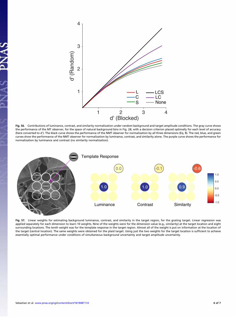
1 2 3 4

(R

ando

m)

1

2

3

4

LCS

S NoneLCC

L

Fig. S6. Contributions of luminance, contrast, and similarity normalization under random background and target amplitude conditions. The gray curve showsthe performance of the MT observer, for the space of natural background bins in Fig. 2B, with a decision criterion placed optimally for each level of accuracy(here converted to d′). The black curve shows the performance of the NMT observer for normalization by all three dimensions (Eq. 5). The red, blue, and greencurves show the performance of the NMT observer for normalization by luminance, contrast, and similarity alone. The purple curve shows the performance fornormalization by luminance and contrast (no similarity normalization).

-1.0

-0.5

0.0

0.5

1.0

Luminance Contrast Similarity

Template Response

1.0 1.0 0.9

-0.1 -0.60.0

Fig. S7. Linear weights for estimating background luminance, contrast, and similarity in the target region, for the grating target. Linear regression wasapplied separately for each dimension to learn 10 weights. Nine of the weights were for the dimension value (e.g., similarity) at the target location and eightsurrounding locations. The tenth weight was for the template response in the target region. Almost all of the weight is put on information at the location ofthe target (central location). The same weights were obtained for the plaid target. Using just the two weights for the target location is sufficient to achieveessentially optimal performance under conditions of simultaneous background uncertainty and target amplitude uncertainty.

Sebastian et al. www.pnas.org/cgi/content/short/1619487114 6 of 7

Fig. S8. Comparison of proportion of hits (statistical power) of the MT and NMT observer for a fixed proportion of false alarms (type I error rate), as a functionof target amplitude, for several false-alarm rates. The statistical power of the NMT observer is much greater than that of the MT observer, especially when thedesired proportion of false alarms is low, which is appropriate under natural conditions where the probability of target present is low.

Sebastian et al. www.pnas.org/cgi/content/short/1619487114 7 of 7