constraining dark matter equation of state with clash...
TRANSCRIPT

Constraining Dark Matter Equation of State with CLASH Clusters
Barbara Sartoris,Andrea Biviano, Piero Rosati and the CLASH team
London, 18 IX 2013 University of Trieste

B. Sartoris
The Equation of state
London, 18 IX 2013
Mon. Not. R. Astron. Soc. 415, L74–L77 (2011) doi:10.1111/j.1745-3933.2011.01082.x
Measuring the dark matter equation of state
Ana Laura Serra1,2! and Mariano Javier L. Domınguez Romero3!1Dipartimento di Fisica Generale ‘Amedeo Avogadro’, Universita degli Studi di Torino, Via P. Giuria 1, I-10125 Torino, Italy2Istituto Nazionale di Fisica Nucleare (INFN), Sezione di Torino, Torino, Italy3Instituto de Astronomıa Teorica y Experimental (IATE), Consejo de Investigaciones Cientıficas y Tecnicas de la Republica Argentina (CONICET),Observatorio Astronomico Cordoba, Universidad Nacional de Cordoba, Laprida 854, X5000BGR Cordoba, Argentina
Accepted 2011 May 20. Received 2011 May 5; in original form 2011 March 9
ABSTRACTThe nature of the dominant component of galaxies and clusters remains unknown. While theastrophysics community supports the cold dark matter (CDM) paradigm as a clue factor in thecurrent cosmological model, no direct CDM detections have been performed. Faber & Visserhave suggested a simple method for measuring the dark matter equation of state that combineskinematic and gravitational lensing data to test the widely adopted assumption of pressurelessdark matter. Following this formalism, we have measured the dark matter equation of statefor the first time using improved techniques. We have found that the value of the equation-of-state parameter is consistent with pressureless dark matter within the errors. Nevertheless, themeasured value is lower than expected because, typically, the masses determined with lensingare larger than those obtained through kinematic methods. We have tested our techniquesusing simulations and we have also analysed possible sources of error that could invalidate ormimic our results. In light of this result, we can now suggest that understanding the nature ofrequires a complete general relativistic analysis.
Key words: equation of state – gravitation – gravitational lensing: strong – gravitationallensing: weak – galaxies: kinematics and dynamics – dark matter.
1 IN T RO D U C T I O N
Strong evidence, from a large number of independent observations,indicates that dark matter is composed of yet-unknown weaklyinteracting elementary particles. Since these particles are requiredto have small random velocities at early times, they are called colddark matter (CDM). Many solutions have been proposed to explainits presence, but its nature remains obscure. Up to the present day,the hypothesis of pressureless dark matter remains experimentallyuntested since laboratory experiments have not yielded positiveresults (Bertone 2010).
Faber & Visser (2006) have conceived a novel approach to cal-culate the density and pressure profiles of the galactic fluid, with noassumptions about their specific form. Such test is based on GeneralRelativity results, the weak-field condition, and the probe particlespeeds involved (photons and stars). In order to carry out an explicitmeasurement of the dark matter equation of state (EoS), we haveapplied this test to galaxy clusters presenting gravitational lensingeffects. The advantage of galaxy clusters over galaxies is their largerdark matter concentrations and their vast spectroscopic data, whichallow to calculate reliable kinematic profiles.
!E-mail: [email protected] (ALS); [email protected] (MJLDR)
2 A R E L AT I V I S T I C EX P E R I M E N T
A static spherically symmetric gravitational field is representedby a space–time metric of the form (Misner, Thorne & Wheeler1973) ds2 = !c2e2"(r) dt2 + dr2/[1 ! 2m(r)G
rc2 ] + r2 d#2, where"(r) = "(r)/c2 and " is the gravitational potential.
Resorting to the Einstein field equations with a consistent staticand spherically symmetric stress-energy tensor, and using the mass-density definition [
!4!$(r)r2 = m(r)], the pressure profiles are
8!G
c4pr(r) = ! 2
r2
"m(r)G
c2r! r ""(r)
#1 ! 2 m(r)G
c2r
$%,
8!G
c4pt(r) = !
G&m"(r) r ! m(r)
'
c2r3
&1 + r ""(r)
'+ · · ·
+"
1 ! 2 m(r)Gc2r
% """(r)
r+ ""(r)2 + """(r)
%, (1)
where pr(r) and pt(r) refer to the radial and tangential pressureprofiles, respectively, which are completely determined by the twofunctions "(r) and m(r). If these two functions are obtained fromobservations, both pressure profiles can be inferred. For a perfectfluid, we expect p = pt = pr.
When analysing data, it is convenient to assume a simplifyinghypothesis. Standard Newtonian physics are obtained in the limit ofGeneral Relativity through the following conditions: (i) the gravi-tational field is weak 2mG
c2r# 1, 2" # c2; (ii) the test probe particle
C$ 2011 The AuthorsMonthly Notices of the Royal Astronomical Society C$ 2011 RAS
1
!
4!"(r)r2 = m(r)
8!G
c4pr(r) = !
2
r2
"
m(r)G
c2 r! r !!(r)
#
1!2m(r)G
c2 r
$%
;
8!G
c4pt(r) = !
G [m!(r) r !m(r)]
c2 r3
&
1 + r !!(r)'
..
.. +
#
1!2m(r)G
c2 r
$"
!!(r)
r+ !!(r)2 + !!!(r)
%
.
2!lens(r) = !(r) +(
m(r)
r2dr ,
w =pr + 2ptc2 3"
"2!lens(r) = 4! "lens(r). and then!lens(r) =
! mlens(r)r2
dr .mlens(r) =
12 mK(r) +
12 m(r).
!(r) =Gmk
r2; m(r) = 2mlens(r)!mk.
mK(< r) = !r #2
r
G
"
d ln "nd ln r
+d ln #2
r
d ln r+ 2$
%
,
ciao
c" 0000 RAS, MNRAS 000, 000–000
Equation of State
Tangential Pressure profile
1
!
4!"(r)r2 = m(r)
8!G
c4pr(r) = !
2
r2
"
m(r)G
c2 r! r !!(r)
#
1!2m(r)G
c2 r
$%
;
8!G
c4pt(r) = !
G [m!(r) r !m(r)]
c2 r3
&
1 + r !!(r)'
..
.. +
#
1!2m(r)G
c2 r
$"
!!(r)
r+ !!(r)2 + !!!(r)
%
.
2!lens(r) = !(r) +(
m(r)
r2dr ,
w =pr + 2ptc2 3"
"2!lens(r) = 4! "lens(r). and then!lens(r) =
! mlens(r)r2
dr .mlens(r) =
12 mK(r) +
12 m(r).
!(r) =Gmk
r2; m(r) = 2mlens(r)!mk.
mK(< r) = !r #2
r
G
"
d ln "nd ln r
+d ln #2
r
d ln r+ 2$
%
,
ciao
c" 0000 RAS, MNRAS 000, 000–000
Density
Mon. Not. R. Astron. Soc. 415, L74–L77 (2011) doi:10.1111/j.1745-3933.2011.01082.x
Measuring the dark matter equation of state
Ana Laura Serra1,2! and Mariano Javier L. Domınguez Romero3!1Dipartimento di Fisica Generale ‘Amedeo Avogadro’, Universita degli Studi di Torino, Via P. Giuria 1, I-10125 Torino, Italy2Istituto Nazionale di Fisica Nucleare (INFN), Sezione di Torino, Torino, Italy3Instituto de Astronomıa Teorica y Experimental (IATE), Consejo de Investigaciones Cientıficas y Tecnicas de la Republica Argentina (CONICET),Observatorio Astronomico Cordoba, Universidad Nacional de Cordoba, Laprida 854, X5000BGR Cordoba, Argentina
Accepted 2011 May 20. Received 2011 May 5; in original form 2011 March 9
ABSTRACTThe nature of the dominant component of galaxies and clusters remains unknown. While theastrophysics community supports the cold dark matter (CDM) paradigm as a clue factor in thecurrent cosmological model, no direct CDM detections have been performed. Faber & Visserhave suggested a simple method for measuring the dark matter equation of state that combineskinematic and gravitational lensing data to test the widely adopted assumption of pressurelessdark matter. Following this formalism, we have measured the dark matter equation of statefor the first time using improved techniques. We have found that the value of the equation-of-state parameter is consistent with pressureless dark matter within the errors. Nevertheless, themeasured value is lower than expected because, typically, the masses determined with lensingare larger than those obtained through kinematic methods. We have tested our techniquesusing simulations and we have also analysed possible sources of error that could invalidate ormimic our results. In light of this result, we can now suggest that understanding the nature ofrequires a complete general relativistic analysis.
Key words: equation of state – gravitation – gravitational lensing: strong – gravitationallensing: weak – galaxies: kinematics and dynamics – dark matter.
1 IN T RO D U C T I O N
Strong evidence, from a large number of independent observations,indicates that dark matter is composed of yet-unknown weaklyinteracting elementary particles. Since these particles are requiredto have small random velocities at early times, they are called colddark matter (CDM). Many solutions have been proposed to explainits presence, but its nature remains obscure. Up to the present day,the hypothesis of pressureless dark matter remains experimentallyuntested since laboratory experiments have not yielded positiveresults (Bertone 2010).
Faber & Visser (2006) have conceived a novel approach to cal-culate the density and pressure profiles of the galactic fluid, with noassumptions about their specific form. Such test is based on GeneralRelativity results, the weak-field condition, and the probe particlespeeds involved (photons and stars). In order to carry out an explicitmeasurement of the dark matter equation of state (EoS), we haveapplied this test to galaxy clusters presenting gravitational lensingeffects. The advantage of galaxy clusters over galaxies is their largerdark matter concentrations and their vast spectroscopic data, whichallow to calculate reliable kinematic profiles.
!E-mail: [email protected] (ALS); [email protected] (MJLDR)
2 A R E L AT I V I S T I C EX P E R I M E N T
A static spherically symmetric gravitational field is representedby a space–time metric of the form (Misner, Thorne & Wheeler1973) ds2 = !c2e2"(r) dt2 + dr2/[1 ! 2m(r)G
rc2 ] + r2 d#2, where"(r) = "(r)/c2 and " is the gravitational potential.
Resorting to the Einstein field equations with a consistent staticand spherically symmetric stress-energy tensor, and using the mass-density definition [
!4!$(r)r2 = m(r)], the pressure profiles are
8!G
c4pr(r) = ! 2
r2
"m(r)G
c2r! r ""(r)
#1 ! 2 m(r)G
c2r
$%,
8!G
c4pt(r) = !
G&m"(r) r ! m(r)
'
c2r3
&1 + r ""(r)
'+ · · ·
+"
1 ! 2 m(r)Gc2r
% """(r)
r+ ""(r)2 + """(r)
%, (1)
where pr(r) and pt(r) refer to the radial and tangential pressureprofiles, respectively, which are completely determined by the twofunctions "(r) and m(r). If these two functions are obtained fromobservations, both pressure profiles can be inferred. For a perfectfluid, we expect p = pt = pr.
When analysing data, it is convenient to assume a simplifyinghypothesis. Standard Newtonian physics are obtained in the limit ofGeneral Relativity through the following conditions: (i) the gravi-tational field is weak 2mG
c2r# 1, 2" # c2; (ii) the test probe particle
C$ 2011 The AuthorsMonthly Notices of the Royal Astronomical Society C$ 2011 RAS
Radial Pressure profile
No direct observations of the EoS have been carried out to confirm the assumption of DM to be pressureless. Bharadwaj & Kar (2003) first proposed that combined measurements of rotation curves and gravitational lensing could be used to determine the equation of state of a galactic fluid.

B. SartorisFaber & Visser 2006 , Lake 2004
Potentials and Mass profiles
4 T. Faber and M. Visser
which, inserted into (20), gives
n(r) = exp
!
! ![r(r)]!"
m[r(r)]
r(r)2drdr
dr
+O
#
$
2mr(r)
%2&'
, (22)
where r(r) is given by the inverse of (21). Since r =r + O[2m/r], the radii in both sets of coordinates are in-terchangeable to the desired order and hence, we can alsogive the refractive index as a function of the curvature co-ordinate r directly:
n(r) = 1!!(r)!"
m(r)
r2dr+O
(
)
2mr
*2
,2mr
!,!2
+
.(23)
This e"ective refractive index entirely determines the tra-jectory of a light ray, i.e. the probe particles of gravitationallensing. Hence, it is the only possible observable of gravi-tational lensing. We note that the refractive index containstwo distinct ingredients, the potential part, !(r), and theintegral over the mass-function,
,
2m(r)/r2 dr.At this point, we conclude that since gravitational lens-
ing observations yield n(r) and rotation curve measurementsyield !(r), combined observations of n(r) and !(r) allowthe separate deduction of !(r) and m(r), and therefore de-scribe the gravitational field of a galaxy in a general relativis-tic sense, without any prior assumptions. The fundamentalprinciple is that the perception of the gravitational field byprobe particles depends on the speed of the probe parti-cles, which manifests itself in the di"erence of observablesn(r) "= !(r).
For convenience and comparability, we define the lens-ing potential as
2!lens(r) = !(r) +
"
m(r)
r2dr , (24)
so that
n(r) = 1! 2!lens(r) +O-
!2
lens
.
. (25)
4.2 Gravitational lensing formalism
The standard formalism of gravitational lensing in weakgravitational fields is based on the superposition of the de-flection angles of many infinitesimal point masses (Schnei-der, Ehlers & Falco 1992, §4.3).
In general relativity, a point mass M is described by theSchwarzschild exterior metric,
ds2 = !)
1! 2Mr
*
dt2 +dr2
1! 2M/r+ r2 d#2 , (26)
which inserted into (23) gives the e"ective refractive index
n(r) = 1 +Mr
!"
Mr2
dr +O(
)
2Mr
*2+
(27)
= 1 +2Mr
+O(
)
2Mr
*2+
. (28)
In the Newtonian limit, this is generally identified with theNewtonian potential,
n(r) = 1! 2!N(r) , (29)
whereas from (27) it is clear that in the general case, therefractive index is only partially specified by the potentialterm. That the mass term of the refractive index of a pointmass is identical to the potential term is a special case ofthe Schwarzschild metric. Keeping this in mind, we proceedto outline the current formalism.
For a point mass, the angular displacement of the grav-itationally lensed image in the lens plane can be calculatedfrom the refractive index (28) (Schneider et al. 1992):
! = 4M"
|"|2, (30)
where " is the vector that connects the lensed image and thecentre of the lens in the 2-dimensional lens plane. Since theextent of a lensing galaxy’s mass distribution is small com-pared to the distance between the light emitting backgroundobject and the lens, as well as compared to the distance be-tween the lensing galaxy and the observer, one assumes thedeflecting mass distribution to be geometrically thin. There-fore, the volume density ! of the lensing galaxy can be pro-jected onto the so-called lens plane, resulting in the surfacedensity $(") which describes the mass distribution withinthe lens plane (Schneider 1985).
The total deflection angle of a lensing mass with finiteextent is then said to be given by the superposition of allsmall angles (30) due to the infinitesimal masses in the lensplane (Schneider et al. 1992):
!(") = 4
"
$("!)" ! "!
|" ! "!|2d2"! . (31)
This equation is the foundation of the gravitational lensingformalism as introduced by Schneider (1985), and Blandford& Narayan (1986).
Since this formalism is based on the assumption thatthe total angle of deflection is caused by the superpositionof point masses – without the notion of pressure at all – itautomatically assumes that the underlying lensing potentialis Newtonian, i.e. !lens = !N. Hence, the lensing potentialand the naively inferred density- or mass-distribution arerelated by (8):
!2!lens(r) = 4! !lens(r) (32)
which implies
!lens(r) =
"
mlens(r)r2
dr . (33)
However, as we argued previously, the lensing potential !lens
is the fundamental observable, and not the density ! whichwas used to construct the formalism. Therefore, for the gen-eral case that does not assume (iii), i.e. !lens "= !N, we notethat
!lens(r) "= !(r) and mlens(r) "= m(r) . (34)
Instead, the deduced mass distribution mlens(r) has to beconsidered as a pseudo-mass similar to that of rotation curvemeasurements. Its physical interpretation can be deducedfrom the definition of the lensing potential (24):
mlens(r) =12mRC(r) +
12m(r) (35)
# 4!
"
/
!+12(pr + 2pt)
0
r2 dr . (36)
c! 2006 RAS, MNRAS 000, 1–8
Lensing approach
1
!
4!"(r)r2 = m(r)
8!G
c4pr(r) = !
2
r2
"
m(r)G
c2 r! r !!(r)
#
1!2m(r)G
c2 r
$%
;
8!G
c4pt(r) = !
G [m!(r) r !m(r)]
c2 r3
&
1 + r !!(r)'
..
.. +
#
1!2m(r)G
c2 r
$"
!!(r)
r+ !!(r)2 + !!!(r)
%
.
2!lens(r) = !(r) +(
m(r)
r2dr ,
w =pr + 2ptc2 3"
"2!lens(r) = 4! "lens(r). and then!lens(r) =
! mlens(r)r2
dr .mlens(r) =
12 mK(r) +
12 m(r).
!(r) =Gmk
r2; m(r) = 2mlens(r)!mk.
mK(< r) = !r #2
r
G
"
d ln "nd ln r
+d ln #2
r
d ln r+ 2$
%
,
ciao
c" 0000 RAS, MNRAS 000, 000–000
Apply Fermat’s principle to the time-like geodesics
Consider an effective refractive index
Kinematic approach
1
mK(r) =r2
G!!
K !4!G
c2
!
(c2"+ pr + 2pt) r2 dr ,
mlens(r) !4!G
c2
!"
c2"+1
2(pr + 2pt)
#
r2 r. .
!K = ! "= !N . (1)$
4!"(r)r2 = m(r)
8!G
c4pr(r) = #
2
r2
%
m(r)G
c2 r# r !!(r)
&
1#2m(r)G
c2 r
'(
;
8!G
c4pt(r) = #
G [m!(r) r #m(r)]
c2 r3
)
1 + r !!(r)*
..
.. +
&
1#2m(r)G
c2 r
'%
!!(r)
r+ !!(r)2 + !!!(r)
(
.
2!lens(r) = !(r) +!
m(r)
r2dr ,
w =pr + 2ptc2 3"
$2!lens(r) = 4! "lens(r). and then!lens(r) =
$ mlens(r)r2
dr .mlens(r) =
12 mK(r) +
12 m(r).
!(r) =Gmk
r2; m(r) = 2mlens(r)#mk.
mK(< r) = #r #2
r
G
%
d ln "nd ln r
+d ln #2
r
d ln r+ 2$
(
,
ciao
c" 0000 RAS, MNRAS 000, 000–000
Using the Jeans equation
1
mK(r) =r2
G!!
K !4!G
c2
!
(c2"+ pr + 2pt) r2 dr ,
mlens(r) !4!G
c2
!"
c2"+1
2(pr + 2pt)
#
r2 dr
!K = ! "= !N . (1)$
4!"(r)r2 = m(r)
8!G
c4pr(r) = #
2
r2
%
m(r)G
c2 r# r !!(r)
&
1#2m(r)G
c2 r
'(
;
8!G
c4pt(r) = #
G [m!(r) r #m(r)]
c2 r3
)
1 + r !!(r)*
..
.. +
&
1#2m(r)G
c2 r
'%
!!(r)
r+ !!(r)2 + !!!(r)
(
.
2!lens(r) = !(r) +!
m(r)
r2dr ,
w =pr + 2ptc2 3"
$2!lens(r) = 4! "lens(r). and then!lens(r) =
$ mlens(r)r2
dr .mlens(r) =
12 mK(r) +
12 m(r).
!(r) =Gmk
r2; m(r) = 2mlens(r)#mk.
mK(< r) = #r #2
r
G
%
d ln "nd ln r
+d ln #2
r
d ln r+ 2$
(
,
ciao
c" 0000 RAS, MNRAS 000, 000–000
1
mK(r) =r2
G!!
K !4!G
c2
!
(c2"+ pr + 2pt) r2 dr ,
mlens(r) !4!G
c2
!"
c2"+1
2(pr + 2pt)
#
r2 dr
!K = ! "= !N . (1)
#!
q2
q1
n(r)$
dr2 + r2 d"2%
= 0 . (2)
&
4!"(r)r2 = m(r)
8!G
c4pr(r) = #
2
r2
'
m(r)G
c2 r# r !!(r)
(
1#2m(r)G
c2 r
)*
;
8!G
c4pt(r) = #
G [m!(r) r #m(r)]
c2 r3
$
1 + r !!(r)%
..
.. +
(
1#2m(r)G
c2 r
)'
!!(r)
r+ !!(r)2 + !!!(r)
*
.
2!lens(r) = !(r) +!
m(r)
r2dr ,
w =pr + 2ptc2 3"
$2!lens(r) = 4! "lens(r). and then!lens(r) =
& mlens(r)r2
dr .mlens(r) =
12 mK(r) +
12 m(r).
!(r) =Gmk
r2; m(r) = 2mlens(r)#mk.
mK(< r) = #r $2
r
G
'
d ln "nd ln r
+d ln $2
r
d ln r+ 2%
*
,
ciao
c" 0000 RAS, MNRAS 000, 000–000
1
n(r) = 1!!(r)!!
m(r)
r2dr+O
"
#
2m
r
$2
,2m
r!,!2
%
.(1)
mK(r) =r2
G!!
K "4!G
c2
!
(c2"+ pr + 2pt) r2 dr ,
mlens(r) "4!G
c2
!&
c2"+1
2(pr + 2pt)
'
r2 dr
!K = ! #= !N . (2)
#!
q2
q1
n(r)(
dr2 + r2 d"2)
= 0 . (3)
*
4!"(r)r2 = m(r)
8!G
c4pr(r) = !
2
r2
"
m(r)G
c2 r! r !!(r)
+
1!2m(r)G
c2 r
,%
;
8!G
c4pt(r) = !
G [m!(r) r !m(r)]
c2 r3
(
1 + r !!(r))
..
.. +
+
1!2m(r)G
c2 r
,"
!!(r)
r+ !!(r)2 + !!!(r)
%
.
2!lens(r) = !(r) +!
m(r)
r2dr ,
w =pr + 2ptc2 3"
$2!lens(r) = 4! "lens(r). and then!lens(r) =
* mlens(r)r2
dr .mlens(r) =
12 mK(r) +
12 m(r).
!(r) =Gmk
r2; m(r) = 2mlens(r)!mk.
mK(< r) = !r $2
r
G
"
d ln "nd ln r
+d ln $2
r
d ln r+ 2%
%
,
ciao
c" 0000 RAS, MNRAS 000, 000–000
Measuring the dark matter EoS L75
speeds are slow compared to the speed of light; and (iii) the pressureand matter fluxes are small compared to the mass-energy density.While the first and second conditions are accomplished by galaxiesin clusters, photons only fulfil the first condition. The third condi-tion is often applied, since it is related to the nature of the dominantcomponent and to the possibility that this is a pressureless fluid.The novel idea introduced by Faber & Visser (2006) is to avoid theassumption of the third condition.
Under condition (i) the tt component of the Ricci tensor is (Misneret al. 1973) !2! " #Rt t , then !2! " 4!G
c2 (c2" + pr + 2pt).Consequently, the function !(r) can be interpreted as the Newtoniangravitational potential !N(r) if and only if the fluid is pressureless.In the kinematic regime, conditions (i) and (ii) are fulfilled. Dueto the second condition, the geodesic equation can be reduced tod2 rdt2 " #!!, where r is the position vector of the galaxy and !(r) $=!N(r). Then, the mass profile obtained from the kinematic analysisis defined by
mK(r) = r2
G!%
K " 4!G
c2
!(c2" + pr + 2pt)r2 dr,
which causes mK(r) to differ from m(r). On the other hand, inthe case of gravitational lensing, photons are the test particles andcondition (ii) is not satisfied. Hence, the geodesic equation needsto be solved exactly to understand the influence of the gravitationalfield. By applying Fermat’s principle and considering an effectiverefractive index (see Faber & Visser 2006 for details), the lensinggravitational potential is defined as
2!lens(r) = !(r) +!
m(r)r2
dr,
where !2!lens(r) = 4!"lens(r), then !lens(r) ="
mlens(r)r2 dr . This
implies mlens(r) = 12 mK(r) + 1
2 m(r). This analysis gives a simpleexpression for the two functions required to calculate the densityand pressure profiles:
!(r) = GmK
r2; m(r) = 2mlens(r) # mK.
It is important to note that a gravitational lensing analysis usu-ally assumes a Newtonian gravitational potential, but in this generalcase, the effective refractive index – a physical observable of grav-itational lensing – requires a more comprehensive definition of thegravitational potential.
3 W E I G H I N G C L U S T E R S O F G A L A X I E S
The Jeans equation offers a direct way to calculate the mass profilevia kinematics:
mK(< r) = # r# 2r
G
#d ln "n
d ln r+ d ln # 2
r
d ln r+ 2$
$,
where mK( < r) is the mass enclosed within a sphere of radiusr, "n is the 3D galaxy number density, # r is the 3D line-of-sight(l.o.s.) velocity dispersion and $ is the anisotropy parameter $ =1 # &v2
% + v&2'/(2&v2
r '). An alternative approach was introduced byDiaferio & Geller (1997), who suggested the possibility of measur-ing cluster masses using only redshifts and celestial coordinates ofthe galaxies. The method they developed, called the caustic tech-nique (CT), allows to calculate the mass profile at radii larger thanthe virial radius, where the assumption of dynamical equilibriumis not valid. In a redshift-space diagram (l.o.s. velocity v versusprojected distances R from the cluster centre), cluster galaxies aredistributed on a characteristic trumpet shape, whose boundaries are
called caustics. Since these caustics are related to the l.o.s. com-ponent of the escape velocity, they provide a suitable measure ofthe cluster mass. The CT is a method for determining the causticamplitude A(r) and then the cluster mass profile (see Diaferio &Geller 1997 and Diaferio 2009 for details). In order to calculate thekinematic mass profile, we have applied the following procedure toa simulated cluster extracted from the Millennium Simulation Run(Springel et al. 2005), and two real rich clusters of galaxies (Comaand CL0024). The galaxy systems were selected based on fourconditions: approximate spherical symmetry, low level of subclus-tering, gravitational lensing data measurements (only weak-lensingreconstruction in the case of Coma) and an important number ofmeasured redshifts of galaxies in order to accomplish our assump-tions. Coma and CL0024 have 1119 and 271 galaxies within thecaustics, respectively.
With the purpose of calculating the mass profile via the Jeansequation, we have used the first steps of the CT to remove interlop-ers, and an adaptive kernel method (described in Diaferio & Geller1997) to estimate the density distribution of galaxies in the redshift-space diagram. In this way, we are able to obtain a 1D profile forthe l.o.s. velocity dispersion # R and the 2D number density profile" (which are simply the second and first moments of the densitydistribution at each R, where R is the projected distance from thecentre). Using in this novel way the estimated density distributionof galaxies allows us to measure # R and " at several radii, in orderto recover the kinematic mass profile with high precision.
In all cases, we have used a King profile to fit the number den-sity profile " and we have followed the procedure described inDıaz et al. (2005) to obtain the 3D number density "n. In orderto determine the velocity dispersion # r, we have applied the Abelinversion technique, assuming $ = 0. The 2D and 3D profiles arein good agreement with the real profiles of the simulated cluster.This indicates that the assumption of $ = 0 is quite adequate. De-spite this good agreement, and in order to quantify the impact of$(r) on the dark matter EoS, we have solved the Jeans equationconsidering three cases: (1) $ = 0 and $(r) determined by a lin-ear fit to (2) the data of the selected simulated cluster and (3) thedata from the most massive clusters of the Millennium Simulation(Springel et al. 2005), up to 1 h#1 Mpc. Fig. 1 shows these threemass profiles, together with the caustic mass profile and the truemass profile [Navarro–Frenk–White (NFW) best fit to the simu-lated data]. The difference between the upper panels reflects theeffect of the number of galaxies tracing the kinematics. To mimica lensing situation, we have projected the mass of the haloes in thefield of the simulated cluster and then we have deprojected the 2Ddensity, assuming that all the mass belongs to one single halo. Thedifferences between the true mass profile and the new ‘fake’ massprofile can be appreciated only at large radii and their best NFWfits are almost indistinguishable.
In the calculation of the EoS, we have combined the tangentialand radial pressure, so w = (pr + 2pt)/c2 3". As shown in Fig. 1,there is a good agreement between the mass profiles of the sim-ulated cluster (except for case 3), implying a null w parameter(Fig. 2 ). When (200 galaxies are used, the w parameter profilesdiffer more significantly. This is mainly due to uncertainties of themass profile and the EoS parameter determinations, which originatefrom the low number of galaxies of this simulated cluster. The kine-matic mass profiles show also some variance due to the presenceof inhomogeneities in the radial distributions of galaxies, related tosubclustering.
In Fig. 2, it can also be seen that, when using the mass profiledetermined via the CT, w adopts a high positive value in the inner
C) 2011 The Authors, MNRAS 415, L74–L77Monthly Notices of the Royal Astronomical Society C) 2011 RAS
In the weak field approximation
London, 18 IX 2013

B. Sartoris
Constraining Dark Matter Equation of State: Serra & Romero 2011
L76 A. L. Serra and M. J. L. D. Romero
Figure 1. Mass profiles of the simulated (extreme left-hand panel with 1000 galaxies and middle left-hand panel with 200 galaxies) and real clusters (Coma,middle right-hand panel, and CL0024, extreme right-hand panel) for cases 1 (red dot–dashed line), 2 (grey continuous line with error bars from bootstrapanalysis) and 3 (orange dash–triple-dotted line, only for simulated clusters) from the CT (green dashed line) and lensing analysis. Lensing profiles are fromKubo et al. (2007) (black continuous line) and Gavazzi et al. (2009) (blue continuous line) in Coma, and from Kneib et al. (2003) (black continuous line) andUmetsu et al. (2010) (blue continuous line) in CL0024. The magenta dotted lines are the NFW kinematic profile from !okas & Mamon (2003) in Coma andthe X-ray-inferred hydrostatic equilibrium mass profile from Ota et al. (2004) in CL0024. In the case of the simulated cluster, the solid cyan line is the NFWfit to the true mass profile, and the kinematic mass profiles were computed by selecting a similar number of galaxies to those for the observed clusters, using amagnitude cut-off.
Figure 2. Dark matter EoS radial profiles, corresponding to the mass pro-files of Fig. 1, with the same conventions. For clarity, we split the EoSparameter determination based on the different mass density profiles ob-tained from lensing analysis. Error bars (at the 1! level) were computedusing bootstrap analysis in the galaxy samples used in the determination ofthe kinematic profile and in the NFW parameters of the dark matter profileinferred from lensing.
regions of the clusters. This might happen because the CT is veryeffective in estimating the mass profile in the outskirts, but it tendsto overestimate it within the virial radius (Serra et al. 2010).
4 M E A S U R E M E N T O F T H E DA R K M AT T E RE oS I N C O M A A N D C L 0 0 2 4
The results of the methods described above show a good agreementbetween the measured profile and the real mass profile in the case of
the simulated cluster, independently of the number of galaxies usedin the computation of the kinematic mass. Our method is slightlysensitive to the anisotropy parameter; to address this problem, wehave calculated the EoS with the kinematic mass drawn from cases1, 2 and 3 (explained in Section 3). The resulting profiles, in Fig. 2,show that the anisotropy parameter " has a non-negligible impacton the EoS. As the first result of this work, we have found, in thecase of the real clusters of galaxies, a good agreement between thekinematic mass profiles computed using the CT (heuristic recipe)and the Jeans equation inversion (rigorously correct), but there isa notable difference between them and the mass derived from thegravitational-lens model (Fig. 1, see also Diaferio 2009). However,this discrepancy allows us to measure the dark matter EoS for thefirst time using clusters of galaxies. The resulting EoS of the darkmatter (shown in Fig. 2) behaves as expected when we analyse thesimulated cluster, but it adopts an almost constant negative valuefor the real clusters (however, consistent with the strong energycondition) instead of the constant zero value required by CDM. Wecould attribute that to the anisotropy parameter ". Nevertheless, theCT is not strongly dependent on ", and the EoS from the causticprofile also shows a trend to be negative. We have checked a numberof sources of systematics such as the departure of sphericity andrelaxation, the presence of deflecting substructures in the l.o.s. (asthose reported in Coma by Adami et al. 2009) and the ellipticityof the halo. We have tested the lack of sphericity by computingthe mass profiles along three different l.o.s., showing no significantdifferences. The presence of substructures in the l.o.s. has beenevaluated not only through the redshift distribution of the clustergalaxies, but also through deprojecting the 2D mass, assuming thatthe mass of the haloes near the l.o.s. belongs to the same cluster(as explained in Section 3). As for the triaxiality of the halo, wehave modified the NFW parameters of the lensing mass, accordingto the results presented in Corless & King (2007), considering anextreme case of the axial ratio Q = 2.5. None of these tests seemsto explain the features we have shown (Serra 2008), although westress that a combination of several of them might be responsiblefor this apparent inconsistency.
It should be mentioned that the cluster of galaxies CL0024 expe-rienced a merger along the l.o.s. (Czoske et al. 2002) approximately2–3 Gyr ago. Nevertheless, the good agreement between the kine-matic mass profile computed and the Ota et al. (2004) hydrostaticalequilibrium mass in the inner region indicates that the gravitational
C! 2011 The Authors, MNRAS 415, L74–L77Monthly Notices of the Royal Astronomical Society C! 2011 RAS
CL 0024 low quality lensing
data low member number kinematical evidence
of merging
L76 A. L. Serra and M. J. L. D. Romero
Figure 1. Mass profiles of the simulated (extreme left-hand panel with 1000 galaxies and middle left-hand panel with 200 galaxies) and real clusters (Coma,middle right-hand panel, and CL0024, extreme right-hand panel) for cases 1 (red dot–dashed line), 2 (grey continuous line with error bars from bootstrapanalysis) and 3 (orange dash–triple-dotted line, only for simulated clusters) from the CT (green dashed line) and lensing analysis. Lensing profiles are fromKubo et al. (2007) (black continuous line) and Gavazzi et al. (2009) (blue continuous line) in Coma, and from Kneib et al. (2003) (black continuous line) andUmetsu et al. (2010) (blue continuous line) in CL0024. The magenta dotted lines are the NFW kinematic profile from !okas & Mamon (2003) in Coma andthe X-ray-inferred hydrostatic equilibrium mass profile from Ota et al. (2004) in CL0024. In the case of the simulated cluster, the solid cyan line is the NFWfit to the true mass profile, and the kinematic mass profiles were computed by selecting a similar number of galaxies to those for the observed clusters, using amagnitude cut-off.
Figure 2. Dark matter EoS radial profiles, corresponding to the mass pro-files of Fig. 1, with the same conventions. For clarity, we split the EoSparameter determination based on the different mass density profiles ob-tained from lensing analysis. Error bars (at the 1! level) were computedusing bootstrap analysis in the galaxy samples used in the determination ofthe kinematic profile and in the NFW parameters of the dark matter profileinferred from lensing.
regions of the clusters. This might happen because the CT is veryeffective in estimating the mass profile in the outskirts, but it tendsto overestimate it within the virial radius (Serra et al. 2010).
4 M E A S U R E M E N T O F T H E DA R K M AT T E RE oS I N C O M A A N D C L 0 0 2 4
The results of the methods described above show a good agreementbetween the measured profile and the real mass profile in the case of
the simulated cluster, independently of the number of galaxies usedin the computation of the kinematic mass. Our method is slightlysensitive to the anisotropy parameter; to address this problem, wehave calculated the EoS with the kinematic mass drawn from cases1, 2 and 3 (explained in Section 3). The resulting profiles, in Fig. 2,show that the anisotropy parameter " has a non-negligible impacton the EoS. As the first result of this work, we have found, in thecase of the real clusters of galaxies, a good agreement between thekinematic mass profiles computed using the CT (heuristic recipe)and the Jeans equation inversion (rigorously correct), but there isa notable difference between them and the mass derived from thegravitational-lens model (Fig. 1, see also Diaferio 2009). However,this discrepancy allows us to measure the dark matter EoS for thefirst time using clusters of galaxies. The resulting EoS of the darkmatter (shown in Fig. 2) behaves as expected when we analyse thesimulated cluster, but it adopts an almost constant negative valuefor the real clusters (however, consistent with the strong energycondition) instead of the constant zero value required by CDM. Wecould attribute that to the anisotropy parameter ". Nevertheless, theCT is not strongly dependent on ", and the EoS from the causticprofile also shows a trend to be negative. We have checked a numberof sources of systematics such as the departure of sphericity andrelaxation, the presence of deflecting substructures in the l.o.s. (asthose reported in Coma by Adami et al. 2009) and the ellipticityof the halo. We have tested the lack of sphericity by computingthe mass profiles along three different l.o.s., showing no significantdifferences. The presence of substructures in the l.o.s. has beenevaluated not only through the redshift distribution of the clustergalaxies, but also through deprojecting the 2D mass, assuming thatthe mass of the haloes near the l.o.s. belongs to the same cluster(as explained in Section 3). As for the triaxiality of the halo, wehave modified the NFW parameters of the lensing mass, accordingto the results presented in Corless & King (2007), considering anextreme case of the axial ratio Q = 2.5. None of these tests seemsto explain the features we have shown (Serra 2008), although westress that a combination of several of them might be responsiblefor this apparent inconsistency.
It should be mentioned that the cluster of galaxies CL0024 expe-rienced a merger along the l.o.s. (Czoske et al. 2002) approximately2–3 Gyr ago. Nevertheless, the good agreement between the kine-matic mass profile computed and the Ota et al. (2004) hydrostaticalequilibrium mass in the inner region indicates that the gravitational
C! 2011 The Authors, MNRAS 415, L74–L77Monthly Notices of the Royal Astronomical Society C! 2011 RAS
Lensing Masses
Kinematic Masses
X-ray Masses
London, 18 IX 2013
B. Sartoris
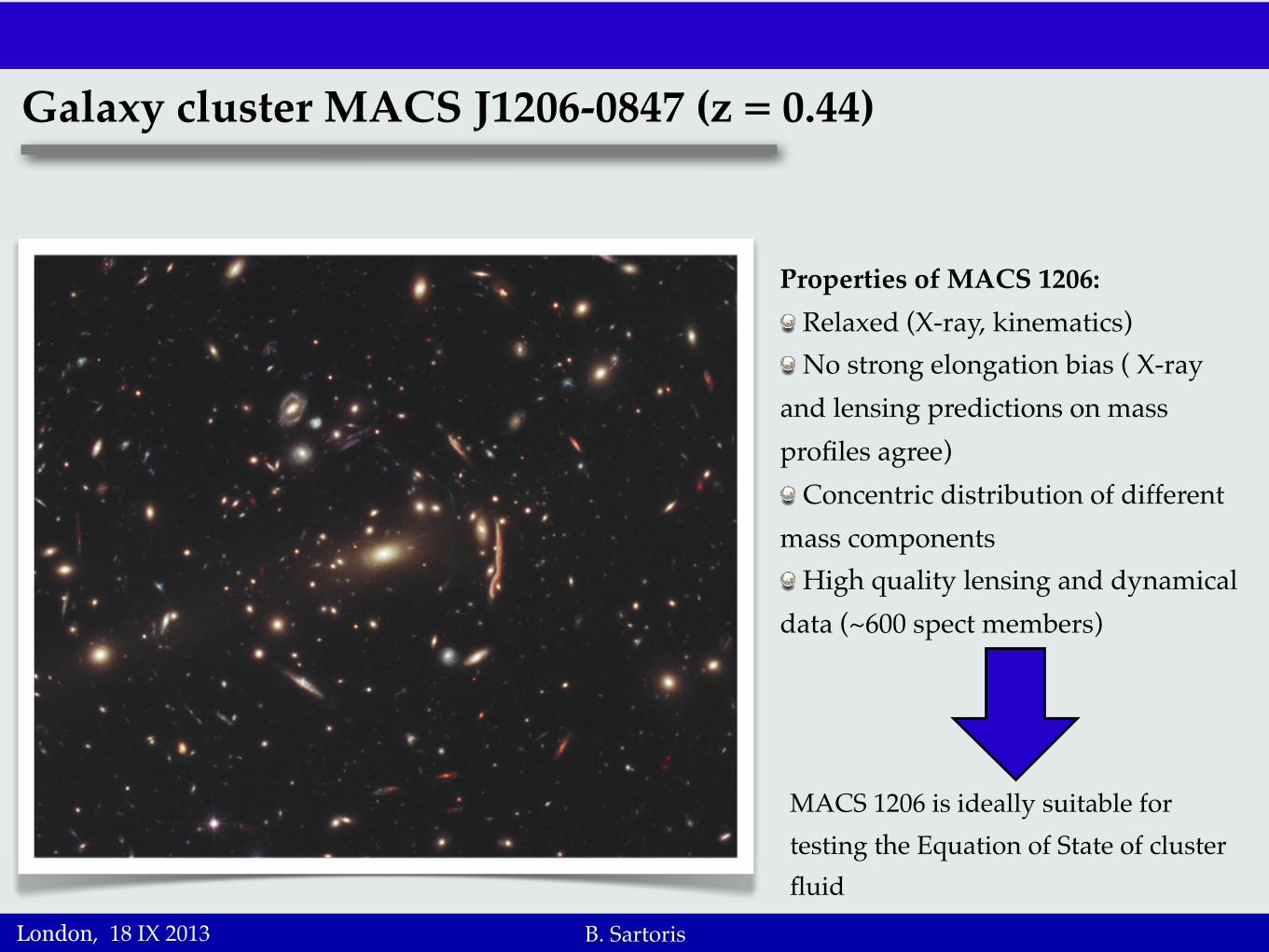
Galaxy cluster MACS J1206-0847 (z = 0.44)
Properties of MACS 1206: Relaxed (X-ray, kinematics) No strong elongation bias ( X-ray
and lensing predictions on mass profiles agree)
Concentric distribution of different mass components
High quality lensing and dynamical data (~600 spect members)
MACS 1206 is ideally suitable for testing the Equation of State of cluster fluid
London, 18 IX 2013

B. SartorisBiviano at al 2013
MACS J1206-0847: Mass profile from kinematicA. Biviano et al.: CLASH cluster mass and velocity anisotropy profiles
Fig. 12. Error ellipses (1 !) and best fit solutions in the M200-c200 space for the NFW M(r) model. Values and errors are listedin Table 3. Lensing analysis of U12: small magenta-filled region(with white border) and white filled dot. MAMPOSSt analysis: blackvertically-elongated contour and filled square. Caustic analysis: greenhorizontally-elongated contour and green diamond. Joint MAMPOSSt+ Caustic constraints: gray-filled region and gray dot with yellow bor-ders. !los+r" analysis: dashed red contours and red cross. The solid(resp. dashed) blue line and shaded cyan region represent the theoret-ical cMr of Bhattacharya et al. (2013) for relaxed (resp. all) halos andits 1 ! scatter. The dash-dotted blue line represents the theoretical cMrof De Boni et al. (2013) for relaxed halos.
derived r200. The best-fit is obtained from a #2-minimizationprocedure. Uncertainties in the best-fit value are obtained usingthe #2 distribution, by setting the e!ective number of indepen-dent data to the ratio between the used radial range in the fit andthe adaptive-kernel radial scale used to determine the caustic it-self. The NFWmodel provides a good fit to the Caustic $(r) overthe full radial range considered (reduced #2 = 0.4).
The r200 and r!2 values obtained with the Caustic method,and their 1 ! errors, are listed in Table 3. For comparison, wealso list in the same Table the adopted results of the MAMPOSStanalysis (Sect. 3.1). The MAMPOSSt and Caustic values of r200and r!2 are consistent within their error bars.
3.3. Combining different mass profile determinations
In Sections 3.1 and 3.2 we have found that the NFW model isthe best description of M(r) among the three we have consid-ered. This is a particularly welcome result because also U12found that the NFW model is a good description to the clusterM(r) obtained by a gravitational lensing analysis. It is thereforestraightforward to compare our results with those of U12.
In Table 3 we list the values of r200, r!2 and of the relatedparameters M200, c200, as obtained from the MAMPOSSt andCaustic analyses (see Sect. 3.1 and 3.2), as well as the resultsobtained by U12. In addition, we list the values obtained by tak-ing error-weighted averages of the MAMPOSSt and Caustic r200
Fig. 13. Top panel: The projected mass profile Mp(R) from the jointMAMPOSSt+Caustic pNFW solution (solid yellow line) within 1 !confidence region (hatched gray region), and from the lensing anal-ysis of U12 (dashed white line: strong lensing analysis; dash-dottedline: weak lensing analysis, after subtraction of the contribution of thelarge-scale structure along the line-of-sight) within 1 ! confidence re-gion (hatched magenta regions). The black triple-dots-dashed line isthe pNFW mass profile from U12’s analysis of Chandra data. The ver-tical dashed line indicates the location of r200,U in both panels. Bottompanel: The ratio between the kinematic and lensing determinations ofMp(R). The white dashed and dash-dotted (resp. solid yellow) line rep-resents the ratio obtained using the non-parametric determination (resp.the pNFW parametrization) of the lensing Mp(R). The pink hatched re-gion represents the confidence region of this ratio for the non-parametricMp(R) lensing solution. The horizontal black dotted line indicates thevalue of unity.
and r!2 values. Even if the two methods are quite di!erent, theyare largely based on the same data-set. To account for this, wemultiply by
"2 the errors on the weighted averages. Combining
the MAMPOSSt and Caustic results allows us to reach an accu-racy on the M(r) parameters which is unprecedented for a kine-matic analysis of an individual cluster, similar to that obtainedfrom the combined strong and weak lensing analysis. There is avery good agreement between the r200, r!2 values obtained by thecombined MAMPOSSt and Caustic analyses and those obtainedby the lensing analysis of U12.
Our kinematic constraints on the cluster M(r) are free of theusual assumptions that light traces mass and that the DM parti-cle and galaxy velocity distributions are identical. When dealingwith poor data-sets (unlike the one presented here) one is forcedto adopt simpler techniques and accept these assumptions. It isinstructive to see what we would obtain in this case. We woulduse the sample of passive members to infer the value of r200 fromthe !los value, as we have done in Sect. 2.1. As for the value ofr!2 we would assume it to be identical to r" (see Sect. 2.2); thisis the so-called ’light traces mass’ hypothesis. There is someobservational support that this assumption is verified (on aver-age) for the passive population of cluster members (e.g. van der
Article number, page 11 of 21
Umetsu at al 2012
X- ray
Lensing (Weak + Strong) (NFW )Kinematic (NFW)
Projected mass profiles :
London, 18 IX 2013
-0.4
-0.3
-0.2
-0.1
0
0.1
0.2
0.3
0.4
0.5 1 1.5 2 2.5 3 3.5 4 4.5
w(r)
r [Mpc]
NFW, `=ONFW, `=CNFW, `=T
B. Sartoris
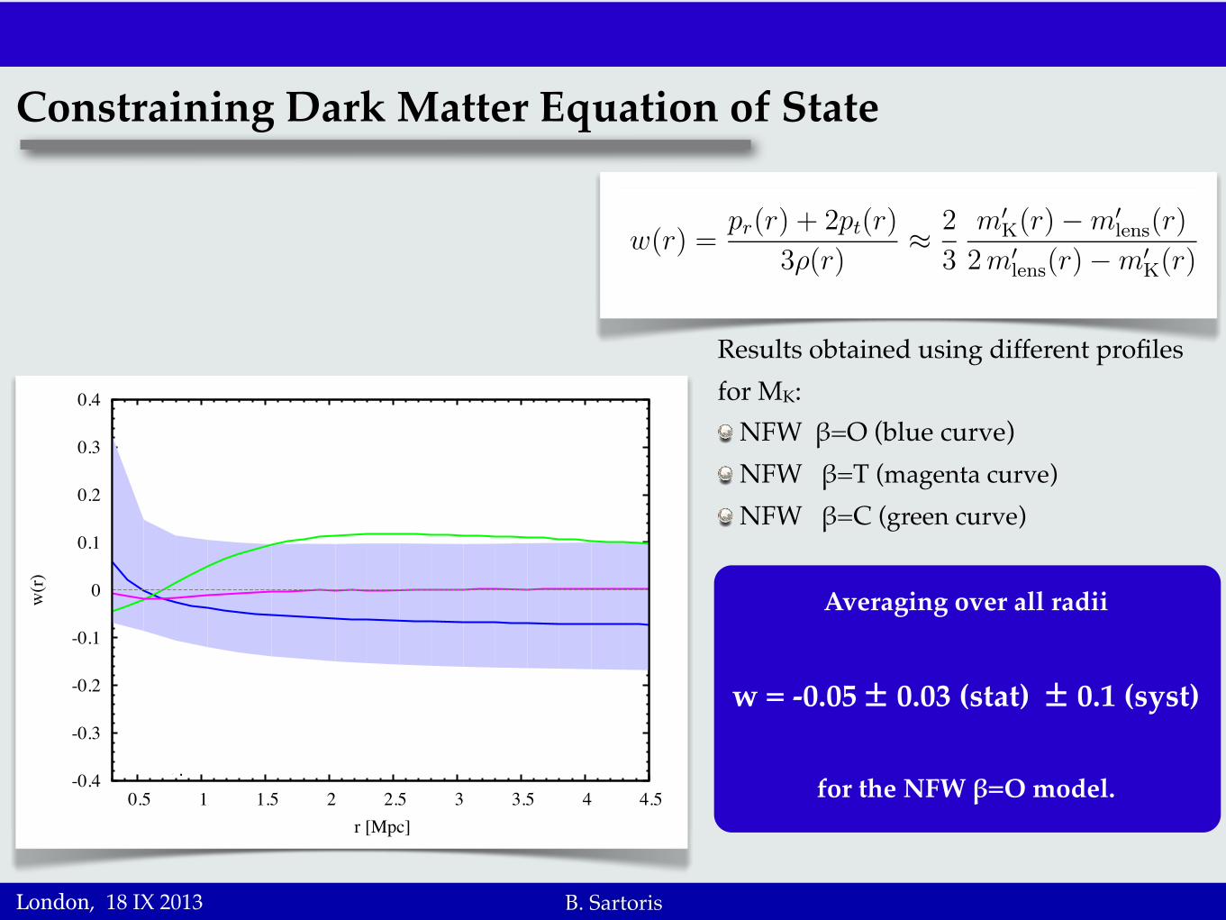
Constraining Dark Matter Equation of State1
w(r) =pr(r) + 2pt(r)
3!(r)!
2
3
m!K(r)"m!
lens(r)
2m!lens(r)"m!
K(r)(1)
!(r) =1
4! r2[2m!
lens(r)"m!K(r)] ,
pr(r) + 2pt(r) !2 c2
4! r2[m!
K(r)"m!lens(r)] .
c" 0000 RAS, MNRAS 000, 000–000
London, 18 IX 2013
Results obtained using different profiles for MK:
NFW !=O (blue curve) NFW !=T (magenta curve) NFW !=C (green curve)
Averaging over all radii
w = -0.05 ± 0.03 (stat) ± 0.1 (syst)
for the NFW !=O model.
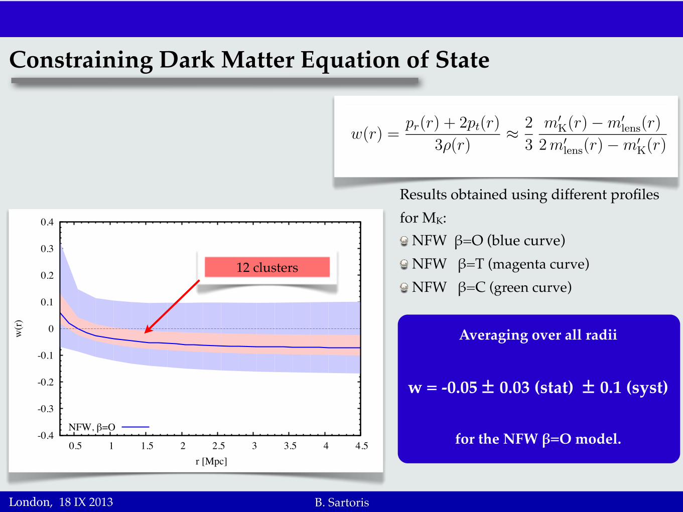
B. Sartoris
Constraining Dark Matter Equation of State1
w(r) =pr(r) + 2pt(r)
3!(r)!
2
3
m!K(r)"m!
lens(r)
2m!lens(r)"m!
K(r)(1)
!(r) =1
4! r2[2m!
lens(r)"m!K(r)] ,
pr(r) + 2pt(r) !2 c2
4! r2[m!
K(r)"m!lens(r)] .
c" 0000 RAS, MNRAS 000, 000–000
London, 18 IX 2013
Results obtained using different profiles for MK:
NFW !=O (blue curve) NFW !=T (magenta curve) NFW !=C (green curve)
Averaging over all radii
w = -0.05 ± 0.03 (stat) ± 0.1 (syst)
for the NFW !=O model. -0.4
-0.3
-0.2
-0.1
0
0.1
0.2
0.3
0.4
0.5 1 1.5 2 2.5 3 3.5 4 4.5
w(r)
r [Mpc]
NFW, `=O
12 clusters
B. Sartoris
Conclusions
By using high quality kinematic and lensing mass analysis of MACS 1206 cluster we have obtained the most stringent constraint on DM EoS to date.
w = -0.05 ± 0.03 (stat) ± 0.1 (syst)
CLASH - VLT final sample will provide the mass estimates for 12 clusters allowing us to further reduce the uncertainties on the DM Equation of state and control the systematics
The possibility of non-negligible pressure fluid introduces a new free parameter into the analysis of combined kinematic and lensing observations.
London, 18 IX 2013