construction, modeling and evaluation of a low loss · pdf fileconstruction, modeling and...
TRANSCRIPT

Construction, Modeling and Evaluation of a Low Loss Motor/Generator for Flywheels
Abstract The application of flywheels (FWs) for energy storage requires generators with low losses, converting electrical energy to rotational energy and vice versa. In order to keep losses low and achieve a high power density, axial-flux generators with air-wound stator are surveyed. A small-scale axial-flux permanent-magnet (AFPM) generator with ironless stator has been designed and constructed. Magnetic field, voltage and frequency have been measured and analyzed. The different losses, occurring in the experimental set-up have been investigated. A model of the magnetic field of the rotor configuration has been created in COMSOL MultiphysicsTM and the simulation results have been compared to measurements of the flux density in the air gap.

Content 1 Introduction ........................................................................................................................ 4 2 Flywheels in General.......................................................................................................... 5
2.1 Historical Applications of Flywheels ......................................................................... 5 2.2 Principles of Flywheel Technology............................................................................ 6 2.3 Improvements of Technology .................................................................................... 8 2.4 Applications for Flywheel Energy Storages (FES) .................................................... 8
2.4.1 FES for Power Supply........................................................................................ 9 2.3.2 FES for Vehicles .............................................................................................. 10
3 Theory .............................................................................................................................. 12 3.1 Magnetic Fields ........................................................................................................ 12 3.2 Field Calculations Using Numerical Methods ......................................................... 18 3.3 Principle of Synchronous Generators (SG).............................................................. 18 3.4 PM Machines............................................................................................................ 25 3.5 Axial-Flux Machines................................................................................................ 25 3.6 Axial-Flux PM Machines with Air-Wound Stator ................................................... 27 3.7 Losses in an AFPM Machine with Air-Gap Winding.............................................. 27
4 The Experimental Set-Up................................................................................................. 29 4.1 Basic Properties of the Experimental FW Generator ............................................... 29 4.2 Simulation with FEM Simulation Tool.................................................................... 30 4.3 The Rotors ................................................................................................................ 33 4.4 The Air-Gap Winding Stator.................................................................................... 34 4.5 The Complete Small-Scale FW Generator............................................................... 36
5 Simulation of the Magnetic Field of the Rotor ................................................................ 38 5.1 The Modeling Software COMSOL Multiphysics™ ................................................ 38 5.2 Geometry Modeling ................................................................................................. 38 5.3 Physics Modeling ..................................................................................................... 39 5.4 Simulation Results.................................................................................................... 40
6 Measurements and Results ............................................................................................... 43 6.1 Measurement of the Magnetic Field of the Rotor .................................................... 43 6.2 Measurement of the Stator Resistance per Phase..................................................... 45 6.3 Measurement of Phase Voltage at Open-Circuit Operation..................................... 45 6.4 Connection of a Load ............................................................................................... 45 6.5 Voltage Harmonics................................................................................................... 46 6.6 Determination of Losses.......................................................................................... 48
6.6.1 Standby Losses................................................................................................. 48 6.6.2 Total Losses...................................................................................................... 52
7 Summary of Results and Discussion................................................................................ 57 7.1 Properties of the Experimental Generator................................................................ 57
7.1.1 Length of Cable in the Winding....................................................................... 57 7.1.2 Mechanical Eigenfrequency............................................................................. 57 7.1.3 Voltage Harmonics........................................................................................... 57 7.1.4 Generator Efficiency ........................................................................................ 58 7.1.5 Stored Kinetic Energy ...................................................................................... 58
7.2 Comparison of Measurement and Simulation Results ............................................. 58 7.2.1 Magnetic Flux Density ..................................................................................... 58 7.2.2 Voltage Output ................................................................................................. 61
7.3 Discussion of the Measurement and Simulation Results ......................................... 61

8 Conclusion and Suggestions for Future Work ................................................................. 63 8.1 Conclusion................................................................................................................ 63 8.2 Suggestions for Future Work ................................................................................... 63
9 Acknowledgements .......................................................................................................... 65 References ................................................................................................................................ 66 Appendix .................................................................................................................................. 68
A Abbreviations ............................................................................................................... 68 B Symbols........................................................................................................................ 69 C Properties of the Sintered NdFeB PM.......................................................................... 71 D Calculation of Polar Mass Moment of Inertia (m-file) ................................................ 72 E Cross Section of the Experimental Generator .............................................................. 74 F Pictures of the Experimental FW Generator ................................................................ 75 G Calculation of Losses of the Experimental Set-Up (m-file)......................................... 76
1 Introduction 4 _________________________________________________________________________________________________________________
1 Introduction The storage of energy can help to increase the efficiency and quality of electrical power supply and traction units e.g. as part of a hybrid propulsion system for vehicles. Due to improvements in material, magnetic bearings and power electronics, flywheels become a reasonable alternative for energy storage. A motor/generator with both low no-load losses and low load losses is needed, as electrical energy has to be converted to mechanical energy and vice versa. Excitation losses are avoidable by using permanent magnets (PMs) instead of electromagnetic poles. Mechanical losses can be kept low by using magnetic bearings and operating the FW in a vacuum vessel. Under low-pressure conditions axial-flux machines have an advantage over radial-flux machines because of their easier cooling arrangements. In electrical machines without ferromagnetic material in the stator, no core losses occur. Thus, coreless stator AFPM generators seem quite suitable for energy storage with flywheels [1]. Connected to the shaft of a flywheel a motor/generator rotates even during standby operation when no electrical energy is absorbed or supplied. The rotating magnetic field of the PMs induces eddy-currents in the stator winding resulting in Joule heating, and consequently losses [2]. During load operation, eddy currents in the PMs and the rotor discs can appear due to the harmonic content of the air-gap flux-density distribution. It is important to estimate the eddy-current losses in the rotor, since the heat generated in the rotor can demagnetize the PMs and cooling is not easy under low-pressure conditions [3], [4], [5]. A motor/generator, which produces high voltage and low current, would be advantageous concerning copper losses. Instead of rectangular conductors with large areas insulated circular conductors (e.g. cables) have to be applied for the stator winding of such a machine [1]. For this thesis a small-scale flywheel motor/generator using cables for the air-gap winding has been designed and constructed. The magnetic field of the rotor configuration has been simulated by modeling the rotor configuration in COMSOL Multiphysics™. Moreover, measurement results from the experimental set-up have been analyzed. In particular it has been examined whether it was possible to determine eddy-current losses in the magnets, the rotor discs and the stator cables by measurements on the experimental set-up.

2 Flywheels in General 5 _________________________________________________________________________________________________________________
2 Flywheels in General A flywheel (FW) is a rotating disc used to store energy in the form of kinetic energy. Modern flywheels are used for storing electric energy and require a motor/generator for energy conversion. 2.1 Historical Applications of Flywheels The flywheel is considered to be one of the earliest inventions of human kind. Simple flywheels have been used as bases for potter´s wheels and grindstones. With the increased utilization of machines, more advanced flywheels have been adopted to achieve smooth operation of machines. For example, they smoothed out the power of steam engines, which were vital for the industrial revolution [1], [6]. In the 1950s the company Oerlikon developed a “gyrobus”. A flywheel of 1,500 kg generated electricity for the electrical motor in the bus. The bus could go approximately 6 km before the flywheel had to be turned up to 3,000 rpm again, taking about 3 minutes. Several busses were in use in Yverdon (Switzerland), Belgium and in the Democratic Republic Congo [7], [8].
a) b) c)
Figure 2.1 Gyrobus [7], [8]
a) A gyrobus getting recharged b) Schematic configuration of the electrical propulsion system when FW getting recharged c) Schematic configuration of the electrical propulsion system with FW as energy source
As early as the late 1800s, a torpedo with flywheel propulsion was developed and built. A flywheel was accelerated up to 12,000 rpm. The power was transmitted to turn propellers, giving the weapon a speed of 30 knots [9], [10].

2 Flywheels in General 6 _________________________________________________________________________________________________________________
2.2 Principles of Flywheel Technology
A flywheel stores kinetic energy of rotation, where the stored energy depends on the polar mass moment of inertia Im and the rotational speed according to:
2
21 ω⋅⋅= mk IE , (2.1)
where Ek: kinetic energy stored
mI : polar mass moment of inertia ω : angular speed.
Connected to an electric motor/generator, a flywheel can be accelerated by the motor when it is supplied with electric energy. Inversely, the generator can provide electrical energy by slowing down the flywheel. In the first case, the flywheel unit absorbs electrical energy, while it delivers electrical energy in the second case. Thus, such a unit can be utilized as storage for electric energy.
Equation (2.1) shows that the energy stored in a flywheel is proportional to the polar mass moment of inertia (i.e. the mass, if equal shapes for different materials are assumed) and to the square of the angular speed. Thus, stored energy can be increased either by choosing a material with higher mass density that leads to high polar mass moment of inertia, or by speeding up the flywheel. Obviously, the latter is the more promising option. Fibre composites are lighter than steel but allow higher rim speeds. Therefore, a good trade-off is gained by using fibre composite instead of steel for the flywheel disc.
The simplest shape of a flywheel is that of a solid cylinder (e.g. a steel rotor). A common shape is a rim attached to a shaft. This shape is often applied if composite materials are used.
Equations (2.2) and (2.3) specify how the polar mass moments of inertia of bodies of these shapes are calculated. It depends on the geometry and the mass.
mm armrI ρπ ⋅⋅⋅⋅=⋅⋅= 42
21
21 , (2.2)
where r: radius of solid cylinder
m: mass of the cylinder a: length of the cylinder ρ m: density of the cylinder material
( 22
41
iom rrmI +⋅⋅= ), (2.3)
where ro: outer radius of a hollow circular cylinder
ri: inner radius of a hollow circular cylinder. The rotational speed is limited by the tensile strength tσ , i.e. the stress developed within the wheel due to inertial loads. At a given speed, lighter materials develop lower inertial loads.

2 Flywheels in General 7 _________________________________________________________________________________________________________________
Since composite materials have a low density and high tensile strength, they enable higher rim speeds for flywheels than steel rotors allow. The maximum energy density of a flywheel with respect to the mass is given by:
m
tm Ke
ρσ
= , (2.4)
where em: kinetic energy per unit mass
K: shape factor tσ : tensile strength mρ : mass density.
The shape factor K that links the maximum energy density to the ratio between maximum tensile strength and the density of the mass depends on the geometry of the flywheel rotor [1], [11]. The values for K vary between 0 and 1. For a flat unpierced disc for example K amounts to 0.606. Table 2.1 shows some examples for other shapes [6]. Table 2.1 Flywheel Geometry Cross section Shape Factor K Constant stress disc 1.000
Modified constant stress disc 0.931
Truncated conical disc
0.806
Flat unpierced disc 0.606
Thin rim
0.500
Rim with web 0.400
Single filament bar
0.333
Flat pierced disc 0.305 So far, energy densities of about 286 kJ/kg have been achieved. It is probable that even much higher energy densities will be possible due to further increase of graphite fiber strength [12]. Especially the high power density compared to chemical batteries makes flywheels useful for applications where high peak power is demanded. Batteries can store a lot of energy, but they cannot be discharged within a very short time without being destroyed. Furthermore, the efficiency decreases considerably for high charge and discharge powers. In contrast, flywheels can easily deliver the whole energy stored within a few seconds, without lowered efficiency or loss of functionality. The number of load cycles is not limited as it is for batteries. A flywheel can also be constructed in different sizes [1], [13].

2 Flywheels in General 8 _________________________________________________________________________________________________________________
Obviously flywheels have to be operated with high revolution speed, in order to achieve high energy and power density. By designing the FW in a way that results in a low eigenfrequency, it can be operated above the corresponding revolution speed. This means that the FW is never slowed down to standstill. But by slowing down a flywheel to e.g. half of the maximum revolution speed, 75% of the total energy is available. One of the disadvantages is the relatively short storage time. While batteries can store energy for years, windage losses, bearing and other losses cause the flywheel to be slowed down, even during standby time. Windage losses can be decreased by operating the flywheel under low-pressure conditions in a vacuum vessel. 2.3 Improvements of Technology The in- and output power is limited by the motor/generator and the power electronics connecting the flywheel unit to a surrounding power system. Due to recent progresses in high-power insulated-gate bipolar transistors (IGBTs) and field-effect transistors (FETs), flywheels can operate at high power with power electronics units comparable in size to the flywheel itself. Thus, flywheels can be used for applications were high peak powers are necessary [1]. As the energy stored in a rotating mass is proportional to the polar mass moment of inertia and to the square of the rotational speed, it is advantageous to have a rotor of strong materials that allow high rotational speed. Instead of steel, modern flywheels consist of carbon fibres. The decrease of stored energy due to lower mass density is overcompensated by much higher rotational speed. Rim speeds up to 1.2 km/s are possible [12]. Magnetic bearings that started to appear in the 1980s enable to reduce the no-load losses considerably. Since magnetic bearing control has been improved, they can replace roller bearings and further more be used to monitor the dynamic behavior of the flywheel. In case of occurrence of abnormal conditions it can be shut down safely [1], [14]. 2.4 Applications for Flywheel Energy Storages (FES) There are two main application areas for flywheels: Grid-connecting applications, e.g. improving power quality, or uninterruptible power supply (UPS) and power supply on several vehicles. Figure 2.2 shows the basic layout of a FES with a motor/generator on the same shaft as the flywheel and enclosed by a vacuum vessel.

2 Flywheels in General 9 _________________________________________________________________________________________________________________
Flywheel rotor
Containment
Bearing
Motor/generator stator
Motor/generator rotor
Vacuum or very low pressure
Bearing
Figure 2.2 Basic layout of a FES [1] 2.4.1 FES for Power Supply Storage of electric energy by flywheels competes with chemical batteries and superconducting magnetic energy storage (SMES). In SMES, energy is stored in the magnetic field surrounding a coil of superconducting wire. The current can circulate in the coil without losses as long as the temperature of the superconducting material is cooled to cryogenetic temperatures. As the cooling consumes energy, long time storage is inconvenient. The practical time to hold energy is in the magnitude of days. For flywheels the practical storage time is even in the range of hours, although FWs rotating for many days have been developed [15]. But the temperature range is much less limited, and the relative size for equivalent power and energy is smaller compared to SMES. Currently, the prices per kilowatt supplied by FWs or SMES are considerably higher than for chemical batteries. On the other hand, further technical development will most likely lower the prices for FWs and SMES, while costs for chemical batteries will probably not become significantly lower than they are at present. Moreover, chemical batteries have disadvantages of possible environmental hazards, lifetime limited to a few years and their state-of-charge being difficult to determine. Taking into consideration that the lifetime of FWs is expected to be more than 20 years, the life-cycle cost of some FW applications are comparable to those of lead-acid batteries. Since FWs can store energy for periods of several hours and can handle high power levels, they are suitable for the use in electrical grids. Due to their short response time, they can be applied to balance the grid frequency. Increasing distributed production of energy by utilizing renewable energy sources raises the demand for short time storages that can compensate for variations in energy production. FWs can contribute to generally improving the power quality in public power supplies. The currently most technically mature commercial application of FWs is the supply of highly reliable electric power for seconds or minutes. For many companies, a short power breakdown can result in huge economical losses, as their production suffers. In some cases, whole production lines might be destroyed, when they are suddenly stopped. One example is the FW energy storage in the combined heat and power station that supplies a semiconductor fabrication facility of Advanced Micro Devices (AMD) in Dresden. While the

2 Flywheels in General 10 _________________________________________________________________________________________________________________
overall power rating of this plant is 30 MW, the FW subsystem can supply or absorb 5 MW for 5 seconds. Thus, it can store up to about 7 kWh. The 5-second storage interval is sufficient for the plant to switch between the utility grid and local generators as power sources. Most power line disturbances last for less than one second. Consequently, uninterruptible power supply (UPS) is possible by using FWs, as they can deliver energy fast and long enough to compensate for short voltage drops or in order to carry the whole load for about 15 seconds, while a standby generator is brought on line [1], [14]. 2.3.2 FES for Vehicles In hybrid electric vehicles, a combustion engine constantly supplies the average power needed to drive the vehicle. Additionally required energy for acceleration and climbing hills is supplied by an electric motor, which takes energy from a temporary store. Thus, the combustion engine can operate at an almost constant optimum speed. Thereby fuel consumption is reduced as well as air and noise pollution. Moreover, the lifetime of the combustion engine is extended. The electric drive motor can be used for regenerative braking. By acting as a generator it can turn the kinetic energy of a vehicle into electric energy charging the store. Consequently, waste heat, as produced by friction brakes, can be decreased. Instead, the energy can be used for subsequent accelerations. So far, nickel metal-hydride batteries are the most common energy storage device in vehicles. But as the energy only has to be stored for relatively short time intervals, they could be replaced by flywheels. Flywheels have longer lifetimes and a higher power and energy density than batteries. While it is difficult to optimize the design of chemical batteries if frequent shallow discharges are mixed with very deep discharges, flywheels operate independently of the depth of discharge. As the current costs for flywheels are higher than the costs for chemical batteries, they are considered preferable in larger vehicles like busses or trains. Hybrid gas turbine/electrical trains are an option to extend high-speed operation to reasonable prices. Trains that are solely diesel-powered are too heavy for speeds higher than about 180 km/h. In contrast, electric trains are quite convenient for operation at high-speed. However, a big drawback is the high costs for electrification. In a hybrid train, the advantages of both propulsion alternatives could be combined. A gas turbine driving a high-speed generator supplies the average power, while a flywheel battery balances the difference between produced electrical energy and the one that is needed for propulsion at a time [14]. Also, in diesel-electric trains for lower speeds, FWs can be applied as energy storage in order to reduce fuel consumption and the environmental impact. Since peak demands on the diesel engine are decreased, it can be sized smaller and thus weight is saved. Further advantages are that the combustion engine can be stopped, although auxiliary devices have to be supplied and emission-free operation on short sections of line e.g. tunnels and stations are possible. Figure 2.3 shows the principle of diesel-electric propulsion. For the Alstom Light Innovative Regional Express (LIREX), a version with flywheels as energy storage has been constructed. The Research Center of Deutsche BAHN AG carried out simulations of the operation of such a version. According to these simulations, about 11% of the energy that a LIREX without flywheels needs can be saved. The shorter the distance between stops, the higher is the saving effect [16], [17].

2 Flywheels in General 11 _________________________________________________________________________________________________________________
If an electrified railroad line exists, the voltage drop at the substations can be reduced by installing FWs in the substations. Additionally, a part of the braking energy can be recovered [14].
Figure 2.3 Principle of propulsion system of a diesel-electric train with energy storage Furthermore, FES can be used for certain military applications. Future combat vehicles will need a lot of electrical power for propulsion, suspension, communication, weapons and defensive systems. One possibility for a hybrid system is an engine providing the power demanded in average combined with fuel cells, supercapacitors and flywheels to supply continous as well as pulsed power. Flywheels designed for applications where power has to be provided within µs would charge a bank of supercapacitors, which then would supply the high-speed systems. The peak power would be several MW. Even higher peak power is required for an electromagnetic aircraft launcher, where 5 to 10 GW are necessary [14]. Moreover, the performance of space vehicles like satellites, planetary rovers or space stations could be improved by equipping them with FES. In earth orbit the sun is the prime energy source, i.e. stored energy is necessary while the space vehicle is in darkness. The initial design for the energy storage on the International Space Station (ISS) uses batteries. It would be advantageous to replace the chemical batteries by flywheels, since they have about the same volume and mass as the batteries but provide energy twice as long and have much longer lifetime. Additionally, the state-of-charge can easily be determined by measuring the rotational velocity. The National Aeronautics and Space Administration (NASA) is developing flywheel sets that can store 15 MJ and deliver a peak power of more than 4 kW. In total, 48 flywheels would be needed to replace all batteries. By doing so, about 100 million Euros could be saved, according to an estimation made by NASA. Taking into account the motor, generator and flywheel losses, the net efficiency (chare-discharge) amounts to 93.7 percent, while the current batteries have an efficiency of about 80 percent [14], [18]. In vehicles like cars, trains and in the ISS, flywheel batteries are controlled as pairs and situated to rotate in opposite direction. If their rotational speed is always changed equally, no net torque will be produced. But in some cases, a net torque might be wanted e.g. in order to supply attitude control. The aim of one program supported by the U.S. Air Force is to develop flywheel-based systems that can store energy and provide torque to a spacecraft [1], [14].

3 Theory 12 _________________________________________________________________________________________________________________ 3 Theory 3.1 Magnetic Fields Electrical charge in motion causes a magnetic field. This moving electrical charge can be a current flowing in a conductor or orbital motions and spins of electrons that are called Ampèrian currents. Such Ampèrian currents exist in permanent-magnet material leading to a magnetization within the material and a magnetic field outside. Ampère´s law relates the magnetic field intensity H to its source the current flowing in a conductor. According to this law the line integral of the magnetic field intensity over any closed loop C spanning the enclosed area A is proportional to the current flow penetrating through this area. If the loop C encloses one conductor (N = 1) with the current I as shown in Figure 3.1 a) this current is equal to the line integral of H along the curve C:
∫ ⋅=⋅C
INsdH , (3.1)
where H : magnetic field intensity
I: electric current N: number of conductors.
a) b)
Figure 3.1 Magnetic field density along a loop enclosing current flowing in conductors a) One conductor carrying current I b) Two conductors carrying current I each
In case of two conductors (N = 2) with identical current I (Figure 3.1 b), two times this current is equal to the line integral. These both conductors could be part of the same coil. The sum of the currents in all conductors penetrating A is called ampere turns or magnetomotive force (mmf) Θ. In case of a number of N conductors carrying the same current I, the magnetomotive force can be calculated according to (3.2).
3 Theory 13 _________________________________________________________________________________________________________________
IN ⋅=Θ , (3.2)
where Θ: ampere turns N: number of conductors
and Ampère´s law can be written as following:
∫ Θ=⋅C
sdH . (3.3)
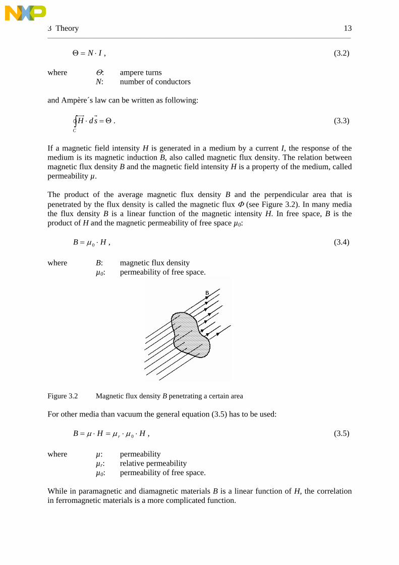
If a magnetic field intensity H is generated in a medium by a current I, the response of the medium is its magnetic induction B, also called magnetic flux density. The relation between magnetic flux density B and the magnetic field intensity H is a property of the medium, called permeability µ. The product of the average magnetic flux density B and the perpendicular area that is penetrated by the flux density is called the magnetic flux Φ (see Figure 3.2). In many media the flux density B is a linear function of the magnetic intensity H. In free space, B is the product of H and the magnetic permeability of free space µ0:
HB ⋅= 0μ , (3.4) where B: magnetic flux density µ0: permeability of free space.
Figure 3.2 Magnetic flux density B penetrating a certain area For other media than vacuum the general equation (3.5) has to be used:
HHB r ⋅⋅=⋅= 0μμμ , (3.5) where µ: permeability µr: relative permeability
µ0: permeability of free space. While in paramagnetic and diamagnetic materials B is a linear function of H, the correlation in ferromagnetic materials is a more complicated function.

3 Theory 14 _________________________________________________________________________________________________________________ The effect that a magnetic material has on the flux density when a field passes through it is represented by the magnetization M. While diamagnets make the flux density smaller, para- and ferromagnets make it larger. How the magnetic flux density is changed by the presence of material is indicated by the relative permeability µr of the material. The magnetization M has the same unit as the magnetic field intensity H:
00 μμB
AM =
⋅Φ
= , (3.6)
where M: magnetization
Φ: magnetic flux. If no external electric currents are present to generate an external magnetic field, the flux density in a magnetic material is simply the magnetization times the permeability. Since magnetization M and magnetic field intensity H contribute to the magnetic flux density in a similar way, their contributions can be summed, when both magnetization and magnetic field are present:
( MHB += 0 )μ . (3.7) The product of magnetization and µ0 is also called magnetic polarization JM. By rearranging (3.5), it is obvious that the permeability is defined as:
HB
=μ . (3.8)
Correspondingly, the susceptibility χ can be defined as:
HM
=χ . (3.9)
Moreover, the relative permeability is defined as:
0μμμ =r . (3.10)
Since the relative permeability is closely related to the susceptibility, the following equation is always true:
1+= χμ r . (3.11) The permeability of free space is
70 104 −⋅⋅= πμ H/m and µr of free space is 1.
While the susceptibility of diamagnetic materials, e.g. copper, is negative, the susceptibility of paramagnetic materials, e.g. aluminium, is small and positive. Typical values are χ =10-3 – 10-5. Ferromagnetic materials have a susceptibility being much greater than one, typically
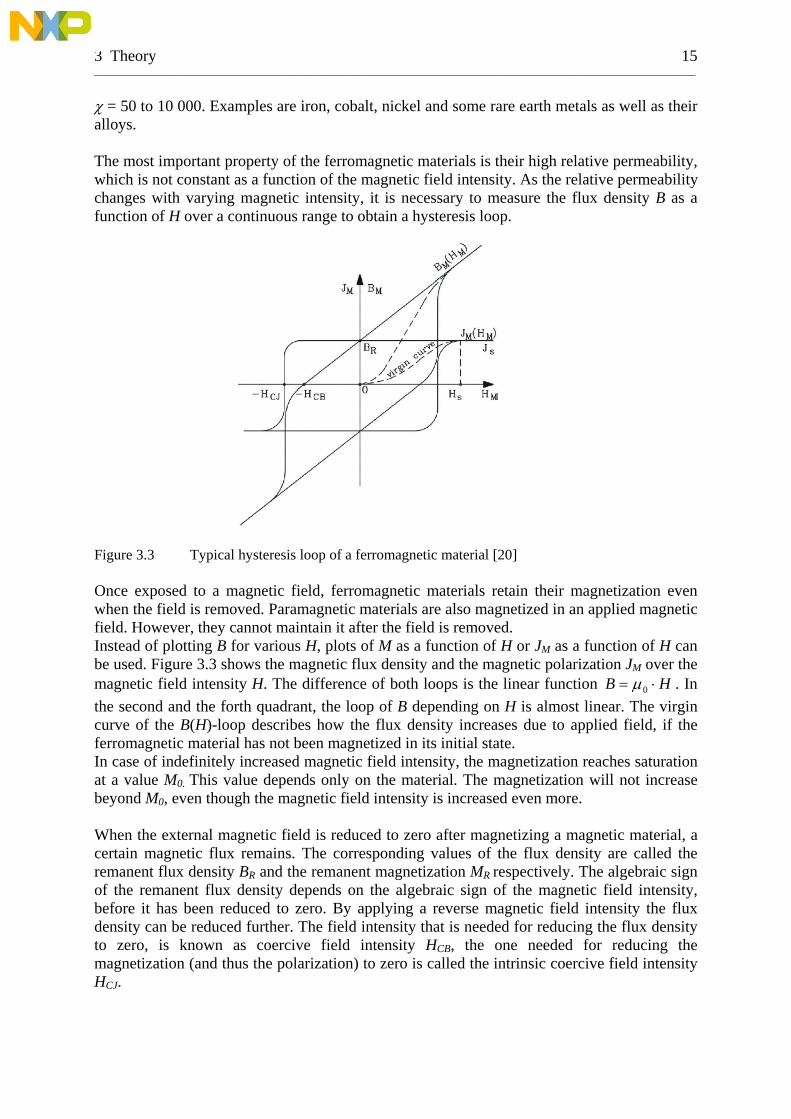
3 Theory 15 _________________________________________________________________________________________________________________ χ = 50 to 10 000. Examples are iron, cobalt, nickel and some rare earth metals as well as their alloys. The most important property of the ferromagnetic materials is their high relative permeability, which is not constant as a function of the magnetic field intensity. As the relative permeability changes with varying magnetic intensity, it is necessary to measure the flux density B as a function of H over a continuous range to obtain a hysteresis loop.
Figure 3.3 Typical hysteresis loop of a ferromagnetic material [20] Once exposed to a magnetic field, ferromagnetic materials retain their magnetization even when the field is removed. Paramagnetic materials are also magnetized in an applied magnetic field. However, they cannot maintain it after the field is removed. Instead of plotting B for various H, plots of M as a function of H or JM as a function of H can be used. Figure 3.3 shows the magnetic flux density and the magnetic polarization JM over the magnetic field intensity H. The difference of both loops is the linear function HB ⋅= 0μ . In the second and the forth quadrant, the loop of B depending on H is almost linear. The virgin curve of the B(H)-loop describes how the flux density increases due to applied field, if the ferromagnetic material has not been magnetized in its initial state. In case of indefinitely increased magnetic field intensity, the magnetization reaches saturation at a value M0. This value depends only on the material. The magnetization will not increase beyond M0, even though the magnetic field intensity is increased even more. When the external magnetic field is reduced to zero after magnetizing a magnetic material, a certain magnetic flux remains. The corresponding values of the flux density are called the remanent flux density BBR and the remanent magnetization MR respectively. The algebraic sign of the remanent flux density depends on the algebraic sign of the magnetic field intensity, before it has been reduced to zero. By applying a reverse magnetic field intensity the flux density can be reduced further. The field intensity that is needed for reducing the flux density to zero, is known as coercive field intensity HCB, the one needed for reducing the magnetization (and thus the polarization) to zero is called the intrinsic coercive field intensity HCJ.

3 Theory 16 _________________________________________________________________________________________________________________ The area enclosed by the hysteresis loop represents the energy expended during one cycle of the hysteresis loop. This energy is also refered to as hysteresis loss. It depends on the coercivity. When a ferromagnetic material is heated it becomes paramagnetic at a certain transition temperature, called the Curie temperature. As the permeability suddenly drops at this temperature, both coercivity and remanence become zero. Ferromagnetic materials can be classified on the basis of their coercivity. Magnetic materials with high coercivity are designated hard magnetic materials and the other soft magnetic materials. An interesting class of magnetic materials are permanent magnets, finding applications in electrical motors and generators. Important properties of these materials are represented by the so-called demagnetization curve. This is the portion of the hysteresis curve in the second quadrant, in which the magnetization is reduced from saturation. The properties depend on the metallurgical treatment and processing of the material and the chemical composition. Besides the coercivity and the remanence, the maximum energy product BHmax is given by the demagnetizing curve. It is obtained by finding the maximum value of the product |BH| in the demagnetizing quadrant of the hysteresis loop. BHmax represents the magnetic energy stored in a permanent-magnet material. However, in most applications, the stability of the permanent magnets is most important. Therefore, the magnets have to be operated sufficiently far below the Curie temperature, as the spontaneous magnetization decreases rapidly with temperature above about 75% of the Curie temperature [19], [20]. Common permanent-magnet materials are Sm2Co17, SmCo5, AlNiCo and Nd2Fe14B [19], [20]. If a conductor carries a current I while a magnetic flux density B is present, a force is exerted on this conductor. The force per meter on the conductor caused by B is given by:
BlIF ×⋅= , (3.12) where F : force on a current-carrying conductor caused by magnetic flux density l : unit vector pointing in the direction of the current. In order to visualize the strength and direction of a magnetic field, so-called lines of magnetic induction are used. They are a geometrical abstraction and always form a closed path. Around a linear current-carrying conductor these lines form loops, being coaxial with the conductor and follow the right-hand rule (see Figure 3.1). In a solenoid the lines are uniform within the solenoid and form a closed return path outside the solenoid. Around a bare magnet, the lines of flux density are similar to those around a solenoid. Both act as magnetic dipoles. Since lines of flux density always form a closed path, the amount of flux entering through any closed surface is equal to the amount of flux leaving it. Thus, the divergence of B is always zero as described by Gauss´ law:
0=⋅∫A
AdB , (3.13)
where A: closed area, where flux density penetrates.
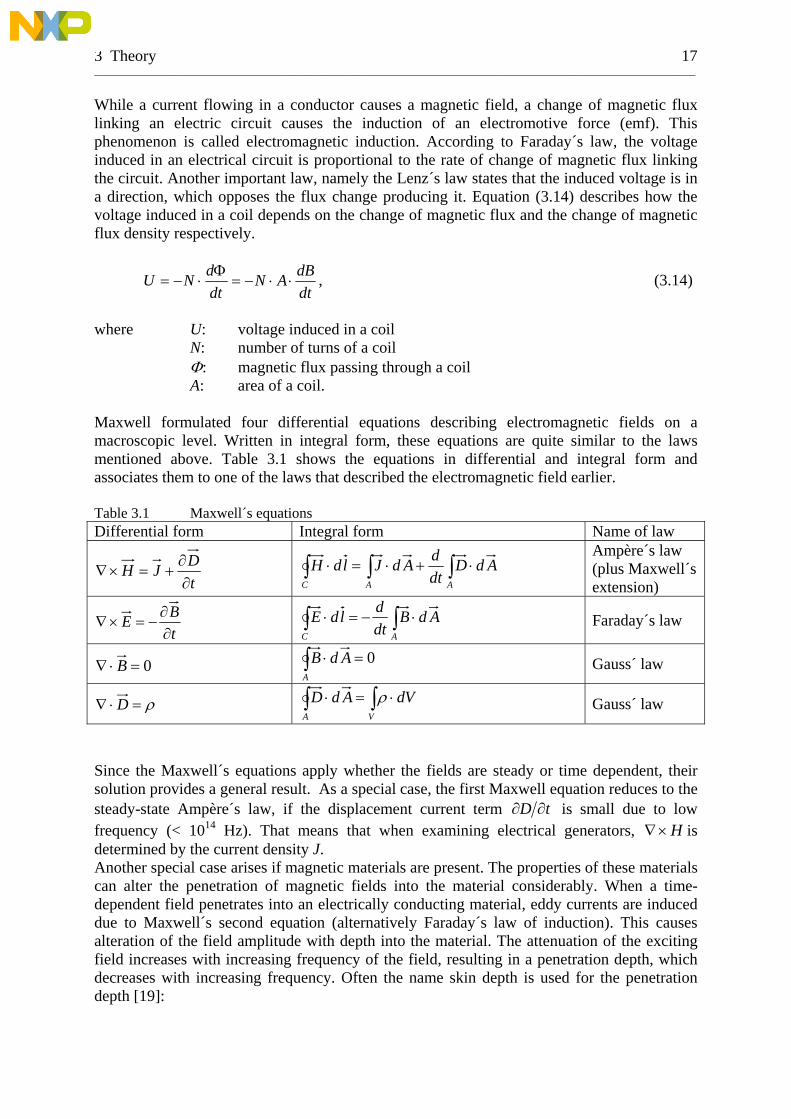
3 Theory 17 _________________________________________________________________________________________________________________ While a current flowing in a conductor causes a magnetic field, a change of magnetic flux linking an electric circuit causes the induction of an electromotive force (emf). This phenomenon is called electromagnetic induction. According to Faraday´s law, the voltage induced in an electrical circuit is proportional to the rate of change of magnetic flux linking the circuit. Another important law, namely the Lenz´s law states that the induced voltage is in a direction, which opposes the flux change producing it. Equation (3.14) describes how the voltage induced in a coil depends on the change of magnetic flux and the change of magnetic flux density respectively.
dtdBAN
dtdNU ⋅⋅−=Φ
⋅−= , (3.14)
where U: voltage induced in a coil N: number of turns of a coil Φ: magnetic flux passing through a coil A: area of a coil. Maxwell formulated four differential equations describing electromagnetic fields on a macroscopic level. Written in integral form, these equations are quite similar to the laws mentioned above. Table 3.1 shows the equations in differential and integral form and associates them to one of the laws that described the electromagnetic field earlier. Table 3.1 Maxwell´s equations Differential form Integral form Name of law
tDJH∂∂
+=×∇ ∫∫∫ ⋅+⋅=⋅AAC
AdDdtdAdJldH
Ampère´s law (plus Maxwell´s extension)
tBE∂∂
−=×∇ ∫ ∫ ⋅−=⋅C A
AdBdtdldE Faraday´s law
0=⋅∇ B ∫ =⋅A
AdB 0 Gauss´ law
ρ=⋅∇ D ∫ ∫ ⋅=⋅A V
dVAdD ρ Gauss´ law
Since the Maxwell´s equations apply whether the fields are steady or time dependent, their solution provides a general result. As a special case, the first Maxwell equation reduces to the steady-state Ampère´s law, if the displacement current term tD ∂∂ is small due to low frequency (< 1014 Hz). That means that when examining electrical generators, H×∇ is determined by the current density J. Another special case arises if magnetic materials are present. The properties of these materials can alter the penetration of magnetic fields into the material considerably. When a time-dependent field penetrates into an electrically conducting material, eddy currents are induced due to Maxwell´s second equation (alternatively Faraday´s law of induction). This causes alteration of the field amplitude with depth into the material. The attenuation of the exciting field increases with increasing frequency of the field, resulting in a penetration depth, which decreases with increasing frequency. Often the name skin depth is used for the penetration depth [19]:

3 Theory 18 _________________________________________________________________________________________________________________
frskin
⋅⋅⋅⋅≈
σμμπδ
0
1 , (3.15)
where δskin: skin depth
σ: electrical conductivity.
3.2 Field Calculations Using Numerical Methods Numerical techniques have to be applied to determine the electric field in complicated configurations. In most cases, Maxwell´s equations have to be solved for a finite region of space, either two- or three-dimensional. Such a finite region of space is called the spatial domain. For solving Maxwell´s equations, an appropriate set of boundary conditions is necessary. Often the magnetic field in the air gap of an electrical machine is to be calculated. Since there are no field sources in the gap the following equations hold:
0=×∇ H
0=⋅∇ B . If field sources occur in the region of interest, the source distribution must be known and included in the calculation. Among others, the finite-difference, the boundary-element method and the finite-element method can be used. In the latter method, the spatial domain is divided into triangle-shaped elements (also other polygonal shapes are possible) and the field values are computed on the nodes of each element. As the size of the elements can be varied over the region of interest, more elements can be included in regions where the field gradient is large [19]. 3.3 Principle of Synchronous Generators (SG) An ordinary three-phase synchronous generator consists of a stator with three-phase current winding (also called armature) and a rotor with a DC field winding that forms a number of poles. This field winding is fed by means of slip rings. The stator winding connected to a three-phase power system excites a rotary current field in the air gap between stator and rotor. Since all SG have an even number of poles, the number of poles divided by two is called the number of pole pairs. Rotor and stator have the same number of pole pairs. Equation (3.16) describes how the rotational speed depends on the electrical frequency and the number of pole pairs.
pfn = , (3.16)
where f: electrical frequency
n: revolution speed p: number of pole pairs.

3 Theory 19 _________________________________________________________________________________________________________________ If the rotor is driven mechanically, the rotor poles induce a three-phase voltage system in the stator winding. When a load is connected current flows in the stator exciting a magnetic field rotating synchronously with the rotor. In case of motor-operation, the three-phase current system in the stator, which excites a rotating field in the air gap, is supplied by the grid. The rotating field attracts the magnetic field of the rotor. Consequently, the rotor rotates with exactly the same speed as the magnetic air-gap field.
a) b) Figure 3.4 Synchronous machine with one phase of the stator winding, salient pole rotor and
magnetic field excited by the rotor winding [21], [22] a) Number of pole pairs p = 1 b) Number of pole pairs p = 2
Figure 3.4 shows the principal construction of a synchronous generator with salient pole rotor, i.e. the rotor poles are formed by a concentrated DC field winding. Alternatively, the field winding can be distributed in many rotor slots. Such a machine with round rotor has a constant air gap. In either case, the stator winding is laid in slots. The magnetic field excited by current flowing in this winding is not exactly sinusoidal, as the winding is not equally distributed but concentrated in the slots. Besides the fundamental wave, the resulting air gap field contains harmonics. There are two common types of stator windings, the lap winding and the wave winding (see Figure 3.5).
a) b) Figure 3.5 Winding schemes for lap and wave winding for a SG with four poles [23]
a) Winding scheme for a lap winding in a stator with 12 slots (3 phases are shown) b) Winding scheme for a wave winding in a stator with 12 slots (1 phase is shown)

3 Theory 20 _________________________________________________________________________________________________________________
a) b)
Figure 3.6 SG with one slot per pole and phase [23]
a) SG with 12 slots in the stator and a rotor with four salient poles b) Voltage phasor diagram for SG with p = 2
As described in (3.16), the electric frequency depends on the revolution speed n as well as on the number of pole pairs p. Assuming the same revolution speed, the electric frequency is twice as high in a SG with p = 2 as in a SG with p = 1. For a 2 pole-pair generator, four poles pass a certain stator slot while the rotor performs one turn, the induced voltage comprises two periods of the fundamental wave. While the mechanical angle between the slots is only 30°, the electrical angle between the voltages in two adjacent slots is 60°. An arrow always pointing on the positive maximum of the fundamental wave of the voltage and initially pointing towards slot 1, points towards slot 7 when the rotor has rotated half a turn. But in slot 1, there is already a positive maximum again, i.e. a whole fundamental wave has been induced in the conductor lying in this slot. Thus, another arrow can be introduced that is now directed to slot 1, primarily pointing towards slot 7. In the slots 1 and 7, another fundamental wave is induced, until the rotor has finished one whole turn. Of course the same applies for all the other slots as well. This is illustrated by the voltage phasor diagram shown in Figure 3.6 b).
a) b) c)
Figure 3.7 SG with 2 slots per pole and phase [23] a) Winding scheme for a lap winding with q = 2 slots per pole and phase b) SG with 12 stator slots and one pole pair c) Voltage phasor diagram for a SG with p = 1 and q = 2

3 Theory 21 _________________________________________________________________________________________________________________ Instead of using one slot per pole and phase (like in Figure 3.5 a)), two or more slots can be used per pole and phase. Applying several slots per pole and phase, results in a more distributed winding. Consequently, the magnetic field becomes more sinusoidal, i.e. its content of harmonics becomes reduced. A winding scheme for a lap winding with q = 2 is shown in Figure 3.7 a). Although the associated SG has only two poles instead of 4, as the one shown in Figure 3.5, the stator has 12 slots, since in total 6 slots per pole are needed. The total number of slots in the stator can be calculated by the following equation:
emqpQ ⋅⋅⋅= 2 , (3.17)
where Q: total number of stator slots q: number of slots per pole and phase
me: number of phases. As shown in Figure 3.7 c), the voltage phasor diagram looks different for a machine with distributed winding. The distances between the tops of the arrows are smaller corresponding to the smaller differences in voltage of two adjacent slots. In Figure 3.8 the arrows connecting the arrowheads of voltage phasors for q = 1 and q = 3 are compared.
Figure 3.8 Voltage phasors [23] The electrical angle between two adjacent slots
pQ
⋅⋅
=πα 2 (3.18)
corresponds to the angle α between the voltage phasors in case of q = 3 in Figure 3.8. The length of phasor AB can be calculated by
⎟⎠⎞
⎜⎝⎛⋅⋅=
2sin2 αRAB . (3.19)
While the arithmetic sum of AB , BC and CD can be calculated by q times AB , the geometric sum is
⎟⎠⎞
⎜⎝⎛ ⋅⋅⋅=
2sin2 αqRAD . (3.20)

3 Theory 22 _________________________________________________________________________________________________________________ By dividing the geometric sum by the arithmetic sum, the so-called distribution factor kd is obtained:
⎟⎟⎠
⎞⎜⎜⎝
⎛⋅⋅
⋅
⎟⎟⎠
⎞⎜⎜⎝
⎛⋅
=
⎟⎟⎠
⎞⎜⎜⎝
⎛⋅⋅
⎟⎟⎠
⎞⎜⎜⎝
⎛⋅⋅
⋅⋅=
⎟⎠⎞
⎜⎝⎛⋅
⎟⎠⎞
⎜⎝⎛ ⋅
=
qmq
m
pQ
q
pQpm
Q
q
qk
e
eed
2sin
2sin
sin
2sin
2sin
2sin
π
π
π
π
α
α
. (3.21)
The fundamental wave of the induced voltage is reduced by this factor but more importantly, the harmonics are reduced to greater extent according to (3.22). As harmonics in principle are disturbing in SG, they should be as low as possible.
⎟⎟⎠
⎞⎜⎜⎝
⎛⋅⋅
⋅⋅
⎟⎟⎠
⎞⎜⎜⎝
⎛⋅
⋅=
qmq
mk
e
ed
2sin
2sin
πν
πν
ν , (3.22)
where ν: number of harmonic q: number of slots per slot and phase
me: number of phases. Another option to reduce harmonics is to design the winding with a coil pitch w smaller than the pole pitch τp. While the latter describes the distance between coil groups of the same phase, the coil pitch (or coil span) describes the distance between conductors of the same coil, like shown in Figure 3.9 a).
a) b)
Figure 3.9 2/3-pitched winding [23] a) Illustration of difference between coil pitch and pole pitch b) Influence of pitch on the third harmonic
Having a coil span shorter than the pole pitch means that a coil encloses a smaller magnetic flux compared to a full-pitch winding. In a single-layer winding, the coil pitch is always identical to the pole pitch, since the length of a pole is determined by the length of the corresponding coils. To enable a shortening of the coil pitch, at least two-layer winding is required (see Figure 3.10).

3 Theory 23 _________________________________________________________________________________________________________________
a)
b)
c) Figure 3.10 Single and two-layer winding distribution [20], [24]
a) Single-layer winding (q = 2) with one coil in each slot b) Two-layer winding (q = 2) with two coils in each slot c) Two-layer winding (q = 3) with two coils in each slot (one phase shown)
Instead of laying one coil in each slot, a second layer of coils with an identical winding scheme can be added. This second layer can be shifted as illustrated in Figure 3.10 b). For the full-pitch winding shown in Figure 3.10 a), the distance between conductor “A” in slot 1 and the closest conductor “A´” (belonging to the same coil) amounts to 6 slot steps. In Figure 3.10 b), the distance between the conductor “A” (upper layer in slot 1) to the closest conductor “A´”(lower layer in slot 6) is only 5 slot steps. Thus, the coil pitch of the winding in Figure 3.10 b) is only 5/6 of the coil pitch of the full-pitch winding. But the pole pitch remains the same. For a SG with two poles, the pole pitch is always half the inner circumference of the stator, i.e. it comprises half the slots. As the ratio between coil pitch and pole pitch in Figure 3.10 b) is 5/6, this winding is called 5/6-pitched winding. If the upper layer was shifted by two slot steps instead of one, it would be a 2/3 pitch. Figure 3.9 b) shows the effect of a 2/3 pitch winding on the 3rd harmonic. With full-pitch winding, e.g. two positive half-waves and one negative half-wave of 3rd harmonic of the magnetic flux are linked with the coil that consists of conductor “a” and “a-“. Since the sum is not zero, voltage with three times the frequency of the fundamental wave is induced. In contrast the sum of flux (ν = 3) linked with a coil of a 2/3-pitched winding is zero. Thus, no voltage is induced due to the third harmonic of the flux.

3 Theory 24 _________________________________________________________________________________________________________________ In general, the effect of pitching of coils is described by the pitch factor kpν according to:
⎟⎟⎠
⎞⎜⎜⎝
⎛⋅⋅=
2sin π
τνν
pp
wk , (3.23)
where w: coil span τp: pole pitch. Since the distribution factor and the pitch factor both describe the reduction of induced voltage for the fundamental wave and each harmonic, they are combined to the winding factor kw:
⎟⎟⎠
⎞⎜⎜⎝
⎛⋅⋅
⋅⋅
⎟⎟⎠
⎞⎜⎜⎝
⎛⋅
⋅⋅⎟⎟⎠
⎞⎜⎜⎝
⎛⋅⋅=⋅=
qmq
mwkkk
e
e
pdpw
2sin
2sin
2sin
πν
πνπ
τνννν . (3.24)
Applying Faraday´s law, the voltage induced in one phase of the stator winding by the magnetic field in the air gap can be calculated according to:
^222 ppwS
wSp BlkNf
kNU ⋅⋅⋅⋅⋅⋅⋅⋅=
Φ⋅⋅⋅= τ
ππ
ω , (3.25)
where NS: number of coil turns per phase
l: length of the machine ^
pB : amplitude of the fundamental wave of the flux density in the air gap. The number of coil turns per phase for a single-layer winding is given by (3.26) and for a two-layer winding it is given by (3.27).
aNqp
N c⋅⋅= (3.26)
aNqp
N c⋅⋅⋅=
2, (3.27)
where Nc: number of turns per coil
a: number of coils connected parallel. The equivalent circuit for a synchronous machine with round rotor is shown in Figure 3.11. RS represents the resistance of the stator winding. US is the voltage between the terminal of one phase and the neutral point and Up is the induced electromotive force due to the fundamental air-gap flux linkage. The stator main reactance Xh and the stator leakage flux reactance Xs can be combined to the synchronous reactance Xd that describes the effect of the total stator magnetic field [20], [23], [24].

3 Theory 25 _________________________________________________________________________________________________________________
Figure 3.11 Equivalent circuit of a synchronous machine with round rotor 3.4 PM Machines Instead of a field winding, permanent magnets can be applied to generate a magnetic field by the rotor. As the rotor does not need to be supplied by any exciting current, no slip rings are necessary. Consequently, there are neither friction losses due to slip rings nor excitation losses in the rotor that would occur even at no-load operation. The relative permeability of the permanent-magnet material is very similar to the one of air, i.e. µr_PM ≅ 1. Therefore, concerning the behavior of the magnetic flux, the air gap of a PM machine with surface mounted magnets can be considered to be constant, like in a round rotor machine, although its geometry looks more like the one of a salient pole machine. Consequently, the same equivalent circuit may be applied as for a round rotor machine [20]. 3.5 Axial-Flux Machines Radial-flux machines, as introduced above, have rotors that rotate within (or in some cases outside) the stator. In contrast, the rotor of an axial-flux machine rotates in a plane, parallel to the stator. In the simplest case, a disc-shaped stator and a rotor disc with PMs are used (see Figure 3.12 a)). In such a single-rotor – single-stator design a strong force of attraction occurs, attracting the rotor towards the stator. Strong bearings would be required to keep the air gap constant [25]. By adding a second stator on the other side of the rotor, the forces in axial direction become balanced (Figure 3.12 b)). Alternatively, a second rotor can be applied. In case of a rotor-stator-rotor structure, the stator has two working surfaces. Consequently, the active conductor length is the sum of the two radial portions that face the magnetic poles of the rotors [26]. Since axial-flux machines have two working surfaces, higher power output can be obtained, compared to radial-flux machines.

3 Theory 26 _________________________________________________________________________________________________________________
a) b) c) Figure 3.12 Axial-flux machines [3]
a) single-rotor – single-stator configuration b) two-stators – one rotor configuration c) two-rotors – one stator configuration
The rotor field is provided by permanent magnets, which either are mounted on the surface of the rotor disc or embedded inside the rotor [27]. The necessary cooling arrangements for an axial-flux machine are simpler than the one for a radial-flux machine, what is of special advantage, when operating under low-pressure conditions [1]. Furthermore, axial-flux machines have a planar adjustable air gap. This can be used for widening the air gap e.g. during the no-load operation of a FW, resulting in reduced losses, while waiting for discharge of energy. As an axial-flux machine has a flat shape, the shaft can be shorter than that of a radial-flux machine. At a high-speed rotation, there is advantage of lower shaft vibrations due to the short length of the shaft. In case of occurring eccentricity, aligning force is generated, reducing radial load [28]. A draw back is the high rotation speed at the outer circumference, since common PM materials have a low tensile strength [1]. For some applications, a reasonable tradeoff can be obtained by applying multi-stage design as shown in Figure 3.13.
a) b)
Figure 3.13 Multi-stage AFPM machine [29]
a) Principal configuration of a multi-stage AFPM machine with three stators b) Path of the main flux in a multi-stage AFPM machine

3 Theory 27 _________________________________________________________________________________________________________________ 3.6 Axial-Flux PM Machines with Air-Wound Stator Because of the varying magnetic field, hysteresis and eddy-current losses occur in the stator iron. Instead of a slotted stator, an air-gap winding can be applied in order to eliminate the iron losses. For instance, an ironless (or coreless) stator can consist of coils that are held together and in position by a composite material of epoxy resin and hardener. According to [30], the fundamental per phase equivalent circuit of a coreless AFPM machine looks like the one shown in Figure 3.14. In this circuit, RS is the stator resistance, LS is the stator inductance and Em represents the induced electromotive force due to the fundamental air-gap PM flux linkage. Ua and Ia are the fundamental instantaneous phase voltage and current respectively. The shunt resistance Re represents the eddy-current loss resistance of the stator.
Figure 3.14 Per-phase equivalent circuit of an AFPM machine 3.7 Losses in an AFPM Machine with Air-Gap Winding While excitation and iron losses are eliminated in an AFPM machine with air-gap winding, there are still some losses both in the rotor and in the stator. Dominating are the resistive copper losses in the stator winding. Further losses are windage losses, bearing losses and losses due to eddy currents. Eddy currents are induced in conducting material when it is subjected to a varying magnetic field. Such currents result in reduction of magnetic flux and power loss. The eddy currents generate Joule heating in the material and extract the necessary energy from the magnetic field [31], [32]. In AFPM a relatively large part of the copper losses is generated in the end windings. Thus, it is advantageous to reduce the length of the end windings by applying a pitched winding [4]. The resistive copper losses in the stator depend only on the current and the resistance of the winding conductors:
SSresistivecopper RIP ⋅= 2_ , (3.28)
where Pcopper_resistive: resistive copper losses in the stator winding IS: phase current of the stator RS: stator phase resistance.
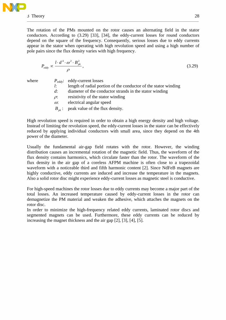
3 Theory 28 _________________________________________________________________________________________________________________ The rotation of the PMs mounted on the rotor causes an alternating field in the stator conductors. According to (3.29) [33], [34], the eddy-current losses for round conductors depend on the square of the frequency. Consequently, serious losses due to eddy currents appear in the stator when operating with high revolution speed and using a high number of pole pairs since the flux density varies with high frequency.
ρω 224
pkeddy
BdlP
⋅⋅⋅∝ , (3.29)
where Peddy: eddy-current losses
l: length of radial portion of the conductor of the stator winding d: diameter of the conductor strands in the stator winding ρ: resistivity of the stator winding ω: electrical angular speed
pkB : peak value of the flux density. High revolution speed is required in order to obtain a high energy density and high voltage. Instead of limiting the revolution speed, the eddy-current losses in the stator can be effectively reduced by applying individual conductors with small area, since they depend on the 4th power of the diameter. Usually the fundamental air-gap field rotates with the rotor. However, the winding distribution causes an incremental rotation of the magnetic field. Thus, the waveform of the flux density contains harmonics, which circulate faster than the rotor. The waveform of the flux density in the air gap of a coreless AFPM machine is often close to a trapezoidal waveform with a noticeable third and fifth harmonic content [2]. Since NdFeB magnets are highly conductive, eddy currents are induced and increase the temperature in the magnets. Also a solid rotor disc might experience eddy-current losses as magnetic steel is conductive. For high-speed machines the rotor losses due to eddy currents may become a major part of the total losses. An increased temperature caused by eddy-current losses in the rotor can demagnetize the PM material and weaken the adhesive, which attaches the magnets on the rotor disc. In order to minimize the high-frequency related eddy currents, laminated rotor discs and segmented magnets can be used. Furthermore, these eddy currents can be reduced by increasing the magnet thickness and the air gap [2], [3], [4], [5].

4 The Experimental Set-Up 29 _________________________________________________________________________________________________________________
4 The Experimental Set-Up A small-scale generator had to be constructed, satisfying the main requirements for a motor/generator for flywheel energy storage: high power output and low losses. Losses appearing during no-load operation reduce the storage time or rather the energy available, at a certain time after charging the FES. Therefore, the design of the constructed generator should aim at minimizing standby-losses. Moreover, the losses of this set-up had to be determined by the means of measurements. A partially constructed generator model existed with some quadratic PM of dimension 20 mm x 20 mm x 10 mm. Instead of completing this one, a new and somewhat larger set-up was constructed. However, the existing model gave suggestions concerning the arrangement of the set-up. The shaft and two wooden columns with the same height as the shaft have been used from the old construction.
Figure 4.1 Pictures of the old set-up 4.1 Basic Properties of the Experimental FW Generator An AFPM machine is applied in order to meet the demand of high power density. A two- rotors – single-stator configuration has been chosen, i.e. one stator is located between two rotor discs with permanent magnets. In order to eliminate hysteresis losses in the stator iron, an ironless stator is used. This means the conductors cannot be laid in slots, properly fixing their position. In such a configuration the magnetic flux passes from one pole on a rotor disc across the air gap with the air-wound stator and through a magnet on the opposite disc. It then it passes along the ferromagnetic rotor disc to the next magnet and returns through the air gap, crossing the stator winding again (see Figure 4.2).
Figure 4.2 Simplified path for the main flux in an AFPM machine with air-gap winding

4 The Experimental Set-Up 30 _________________________________________________________________________________________________________________
Further losses that have to be considered are resistive copper losses, i.e. losses because of the ohmic resistance of the stator winding. Since these losses depend on the current and the resistance of the winding, according to (3.28), there are two possibilities to reduce the losses. Either a conductor with large cross section area is chosen, thus decreasing the resistance, or a cable that enables high voltage, resulting in lower current, is used. The eddy-current losses in the stator winding, which also occur during no-load operation, depend on the 4th power of the diameter of a round conductor (3.29). In addition, increasing the amount of conducting material in the stator increases the weight and the costs of the machine. Therefore, conductors with large diameter are not a reasonable option. The magnetic field generated by the PMs rotates with the rotor discs and the magnets mounted on their surface. However, there will be flux changing in the rotors and the PMs, because the air-gap field, to which the stator also contributes, contains harmonics. Since these harmonics revolve with higher speed than the rotors, magnetic flux changes relative to the rotor discs with the PMs. Consequently, eddy currents are induced in the ferromagnetic material of the rotor discs and the PMs, in case of PMs having high conductivity. Especially at high revolution speeds, theses losses become important, as they depend on the square of the frequency. Reducing the content of harmonics in the air-gap field, results in lower eddy-current losses in the rotor discs and the PMs. 4.2 Simulation with FEM Simulation Tool In order to get a rough idea about the order of magnitude of electric characteristics that can be achieved on the small-scale FW generator, a FEM simulation tool was used. This program is programmed for the simulation of radial-flux PM machines. The geometry of the rotor and the stator can be modelled. For example different PMs (shape, material) and pole shoes (different shapes or no at all) can be chosen for the rotor. The design of the stator slots and the stator cables can be modelled (e.g. area, outer diameter, number of strands). Different pitches and numbers of slots per pole and phase can be chosen. Moreover, the dimensions of rotor, stator and air gap have to be specified. Values for revolution speed, frequency, voltage and apparent power have to be determined. The program executes the calculation only for the smallest section that is symmetrically repeated in the geometry of the machine. It provides values for e.g. the current and length of the machine and shows the magnetic field under no-load conditions as well as under load conditions. Since it is not possible to choose the geometric configuration of an axial-flux machine, a radial-flux machine, as similar as possible to the designated design of the AFPM machine was simulated.

4 The Experimental Set-Up 31 _________________________________________________________________________________________________________________
a) b)
Figure 4.3 Radial- and axial-flux machines with different dimensions but same pole pitch
a) Machines with 4 poles of pole pitch τp and diameter d b) Machines with 8 poles of the same pole pitch τp and diameter d´ = 2·d
Figure 4.3 a) shows the simplified flux density in the air gap for one pole of a radial-flux and an axial-flux machine respectively. Figure 4.3 b) shows both machines with twice the diameter, against which the width of one pole is the same, resulting in twice the amount of poles. The air-gap fields of these two enlarged machines look more similar than the air-gap fields of the smaller machines. The larger both machines are dimensioned, the more similar become the circumstances in the air gap. This has been utilized for the simulation in the FEM simulation tool, by modeling a machine with ten times the dimension of the experimental set-up, as an approach of its properties. Of course, several electrical characteristics are scaled as well. This has to be taken into account, when evaluating the simulation results. Table 4.1 compares the dimensions and characteristics of the design used in the experimental set-up to the one used in the simulation. As the number of pole pairs was not part of the input data, it is not mentioned in the table. However, it depends on the given frequency and revolution speed. For the experimental set-up, the number of pole pairs p was 14, resulting in p = 140 for the in FEM model.
4 The Experimental Set-Up 32 _________________________________________________________________________________________________________________
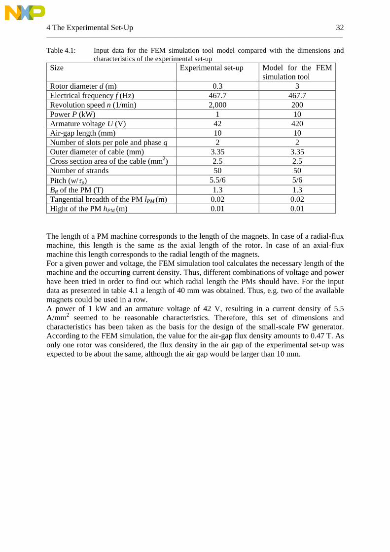
Table 4.1: Input data for the FEM simulation tool model compared with the dimensions and characteristics of the experimental set-up
Size Experimental set-up Model for the FEM simulation tool
Rotor diameter d (m) 0.3 3 Electrical frequency f (Hz) 467.7 467.7 Revolution speed n (1/min) 2,000 200 Power P (kW) 1 10 Armature voltage U (V) 42 420 Air-gap length (mm) 10 10 Number of slots per pole and phase q 2 2 Outer diameter of cable (mm) 3.35 3.35 Cross section area of the cable (mm2) 2.5 2.5 Number of strands 50 50 Pitch (w/τp) 5.5/6 5/6 BBR of the PM (T) 1.3 1.3 Tangential breadth of the PM lPM (m) 0.02 0.02 Hight of the PM hPM (m) 0.01 0.01
The length of a PM machine corresponds to the length of the magnets. In case of a radial-flux machine, this length is the same as the axial length of the rotor. In case of an axial-flux machine this length corresponds to the radial length of the magnets. For a given power and voltage, the FEM simulation tool calculates the necessary length of the machine and the occurring current density. Thus, different combinations of voltage and power have been tried in order to find out which radial length the PMs should have. For the input data as presented in table 4.1 a length of 40 mm was obtained. Thus, e.g. two of the available magnets could be used in a row. A power of 1 kW and an armature voltage of 42 V, resulting in a current density of 5.5 A/mm2 seemed to be reasonable characteristics. Therefore, this set of dimensions and characteristics has been taken as the basis for the design of the small-scale FW generator. According to the FEM simulation, the value for the air-gap flux density amounts to 0.47 T. As only one rotor was considered, the flux density in the air gap of the experimental set-up was expected to be about the same, although the air gap would be larger than 10 mm.

4 The Experimental Set-Up 33 _________________________________________________________________________________________________________________
Figure 4.4 Plot of the field lines and the flux density (in T) of one pole, simulated with the FEM
simulation tool (rotor with PM on the left side and stator slots with cables on the right side)
4.3 The Rotors Both rotors consist of identical discs of ferromagnetic steel. Their outer diameter amounts to 31.5 cm and they are 10 mm thick. Along their outer circumference, they have a rim, 3 mm high and 7.5 mm broad, in order to counteract the centrifugal force that accelerates the PMs outwards.
a) b) c) Figure 4.5 Rotor disc and PMs
a) Rotor disc, how it would look with rectangular magnets b) Rotor disc with conical magnets and almost constant gap between them a) Shape of one single PM with dimensioning
Placing two of the quadratic PMs in a row would result in a relatively large gap between the magnets at the outside of the machine, while the gap would become quite narrow at the inside. A gap between the magnets - much smaller than the air gap - means that a considerable part of the magnetic flux would not pass across the air gap but pass to an adjacent magnet. Since the air-wound stator has to fit between the rotors, the air gap will be quite large. Hence the gap between the magnets must not be smaller than inevitable. This is only possible if conical

4 The Experimental Set-Up 34 _________________________________________________________________________________________________________________
magnets are used. Therefore, custom-made conical NdFeB-magnets with an average width of 20 mm and a height of 10 mm have been applied. On each rotor disc, 28 (two times the number of pole pairs) PMs have been sticked with a two-component adhesive. As PM material, sintered Neodymium-Iron-Boron (NdFeB) with a remanent flux density BBR = 1.3 T is used. Although the Curie temperature of this material is higher than 300 °C, the maximum working temperature amounts to only 80 °C. The value of energy product |BH|max is 320 kJ/m . Further properties of the used PM are given in appendix C. 3
As illustrated in Figure 4.2, approximately half of the flux passing a magnet, continues through the disc by turning to the left and half of it continues in opposite direction. The thickness of the rotor discs amounts to half the average width of the magnets. Thus half the cross section area is available for half the flux, resulting in a nearly constant flux density. 4.4 The Air-Gap Winding Stator Since an ironless stator was required, a material with high electrical resistivity was needed as a base on which the cables of the winding could be laid. Moreover, it should be quite stiff in order to avoid deflection, which could result in demolition of the winding in case of being touched by the fast spinning lower rotor disc. As bakelite meets these two demands fairly well, a 3 mm thick bakelite disc was chosen as base. Further requirements on the stator were arrangements to reduce harmonics in the air-gap field that means a distributed and pitched winding was necessary. Thus, the winding had to be a two-layer winding with at least two slots per pole and phase. While usually coils incorporated in resin (see Figure 4.6) are used for the ironless stator of an AFPM machine, cables with polyolefine insulation have been applied as stator conductors for the experimental FW generator. The eddy-current losses in the winding can be kept low by using a cable with several thin strands.
a) b)
Figure 4.6 Air-gap winding [35]
a) Stator coils incorporated in resin b) Trial winding with cables
The number of poles had been chosen in a way so that the formation of cables would be close-packed with hardly any space between them if the number of slots per pole and phase is 2.
4 The Experimental Set-Up 35 _________________________________________________________________________________________________________________
A higher value of q is not possible, while maintaining a reasonable number of poles. The pole pitch at the middle of the radial length of the magnets is somewhat less than 30 mm. At the inner edge of the magnets it is only 24.7 mm. Thus, 4.1 mm per cable are available per cable, if 6 cables per pole are used. The applied cable has an outer diameter of 3.35 mm and consists of fifty strands. In order to fix them on the bakelite disc, a glue gun and hot-melt adhesive was used. Any deviation from radial and horizontal alignment of the cables in the area between the magnets would influence the content of harmonics. By means of a CNC-miller, 168 very shallow notches have been milled into the bakelite disc. This should ease straight and radial alignment of the cables of the lower layer.
a) b)
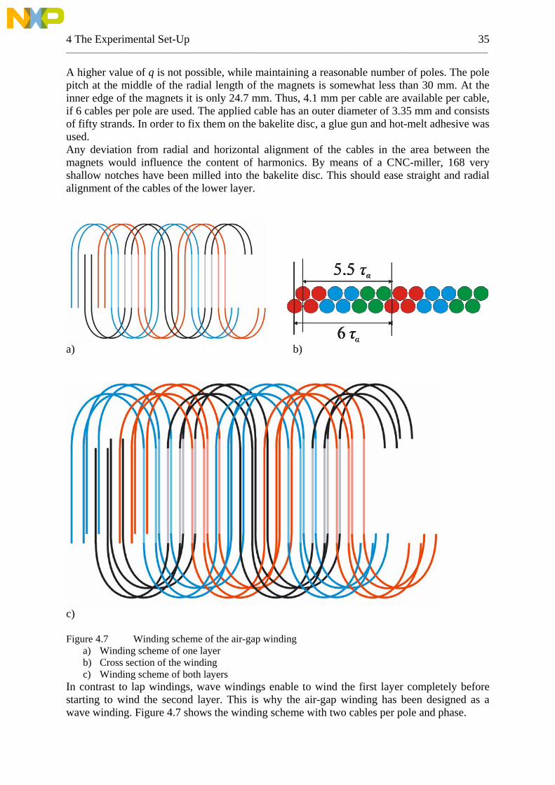
c) Figure 4.7 Winding scheme of the air-gap winding
a) Winding scheme of one layer b) Cross section of the winding c) Winding scheme of both layers
In contrast to lap windings, wave windings enable to wind the first layer completely before starting to wind the second layer. This is why the air-gap winding has been designed as a wave winding. Figure 4.7 shows the winding scheme with two cables per pole and phase.

4 The Experimental Set-Up 36 _________________________________________________________________________________________________________________
Since the upper winding has been laid in the flute between the cables of the lower layer, it is shifted by half a slot step compared to the lower layer. This results in a pitch of 5.5/6 = 11/12, as illustrated in Figure 4.7 b). To obtain an air-gap winding, being as thin as possible, the cables had to be pressed fairly strong against the base, alternatively against the lower layer, in order to avoid having too much adhesive between the cables. In addition the cables had to be laid in their positions properly in order to prevent them becoming bended in the area situated between the magnets. Another challenge was the end-winding part inside the magnets, which is quite narrow. As the bows of several cables cross each other in that area, there was a risk that this part would become very thick, thus increasing the minimum air gap. Figure 4.8 shows the winding on the bakelite disk. Serial connection is applied for all cables belonging to the same phase.
Figure 4.8 Picture of the two-layer air-gap winding on a bakelite disc 4.5 The Complete Small-Scale FW Generator The lower rotor disc is attached to a shaft, which is supported by two ball bearings at its lower end and its upper part. The second rotor disc is fixed by four thread rods, which are inserted in tapped holes in the lower disc. The bakelite with the air-gap winding is bond on a plastic tube. A second plastic tube enclosing both rotor discs and the stator, serves as protection in case of hurtling parts. An allen screw is fixed on the top of the shaft. Thus, a drilling machine with inserted allen key can be used for driving the generator. In Table 4.2 the polar mass moment of inertia and the mass of the rotating parts of the FW are shown. For the calculations, see Appendix D. Figure 4.8 shows the outline and pictures of the whole experimental set-up. In Appendix E the outline with dimensioning is shown. Table 4.2 Polar mass moment of inertia and mass of rotating parts Part Polar mass moment
of inertia (kg·m2) Mass (kg)
Rotor disc (one) 0.0788 6.21 PMs (all) 0.0589 3.36 Other individual rotating parts (e.g. shaft, thread rods)
0.0024 0.77
All rotating parts 0.2189 16.53

4 The Experimental Set-Up 37 _________________________________________________________________________________________________________________
a)
b) c) Figure 4.8 The experimental set-up
a) Outline of the experimental FW generator b) Picture of the stator mounted on a plastic tube and the lower rotor disc with inserted thread
rods for holding the upper rotor disc in place c) Picture of the whole experimental set-up with outer plastic tube as protection
More pictures of the experimental AFPM generator with air-gap winding are shown in Appendix F.
5 Simulation of the Magnetic Field of the Rotor 38 _________________________________________________________________________________________________________________
5 Simulation of the Magnetic Field of the Rotor 5.1 The Modeling Software COMSOL Multiphysics™ COMSOL Multiphysics™ is a software for modeling and solving scientific and engineering problems based on partial differential equations (PDEs). Instead of having models for only one type of physics, it enables models that can solve coupled physics phenomena without requiring in-depth knowledge of numerical analysis. Basically, a model can be built by creating the geometry and defining the relevant physical quantities such as material properties or sources, while COMSOL Multiphsycis™ provides modules for different application areas (e.g. heat transfer, structural mechanics) with respective underlying equations and specialized solvers for the models. For simulations in this thesis the electromagnetic module was used. This module is suitable for simulating electromagnetic wave and field propagation as well as AC-DC electromagnetics. A geometry model contains so-called manifolds, which are defined as mathematical functions describing a surface, curve, or point in a geometry model of any dimension [36]. A domain is a topological entity describing bounded parts of such manifolds as well as relations between manifolds. A domain of dimension one less than the space dimension for the respective model, is termed boundary. For example a face, i.e. a bounded part of a surface, in a 3D geometry is a boundary. Consequently, a subdomain is a topological part of the modelling space. Dependent on the dimension of the modelling space the geometrical representation of a subdomain is either a line segment (in 1D), an area (2D), or a volume (3D). For more detailed definitions see [36]. Since COMSOL Multiphysics™ in principle is unitless, any consistent set of units can be used. But for the Maxwell equations that use the constants for permittivity and permeability in a vacuum ε0 and μ0 the use of SI units is assumed. This has to be taken into account if another unit system than the SI units is chosen. In the simulations with COMSOL Muliphysics™ for this thesis SI units have been used. 5.2 Geometry Modeling In order to reduce the calculation work, only a forth, i.e. seven pole pairs, of the generator was simulated. As the magnetic flux that goes through one specific pole pair returns partly via poles close by, it is necessary to consider more than one pole pair. By taking into account seven pole pairs, there is one pole in the middle having three vicinal pole pairs on each sides. The flux returning via even more distant poles is expected to be negligible compared to the total flux through one pole. The relevant parts of the experimental set-up for the simulation of the magnetic field are the permanent magnets and the rotor discs. All other parts can be ignored as they do not significantly influence the magnetic field. The bakelite disk and the insulation of the cable as well as the copper conductor have a magnetic permeability close to the one of free space µ0. Therefore, the whole stator is considered to have the same magnetic properties as free space.
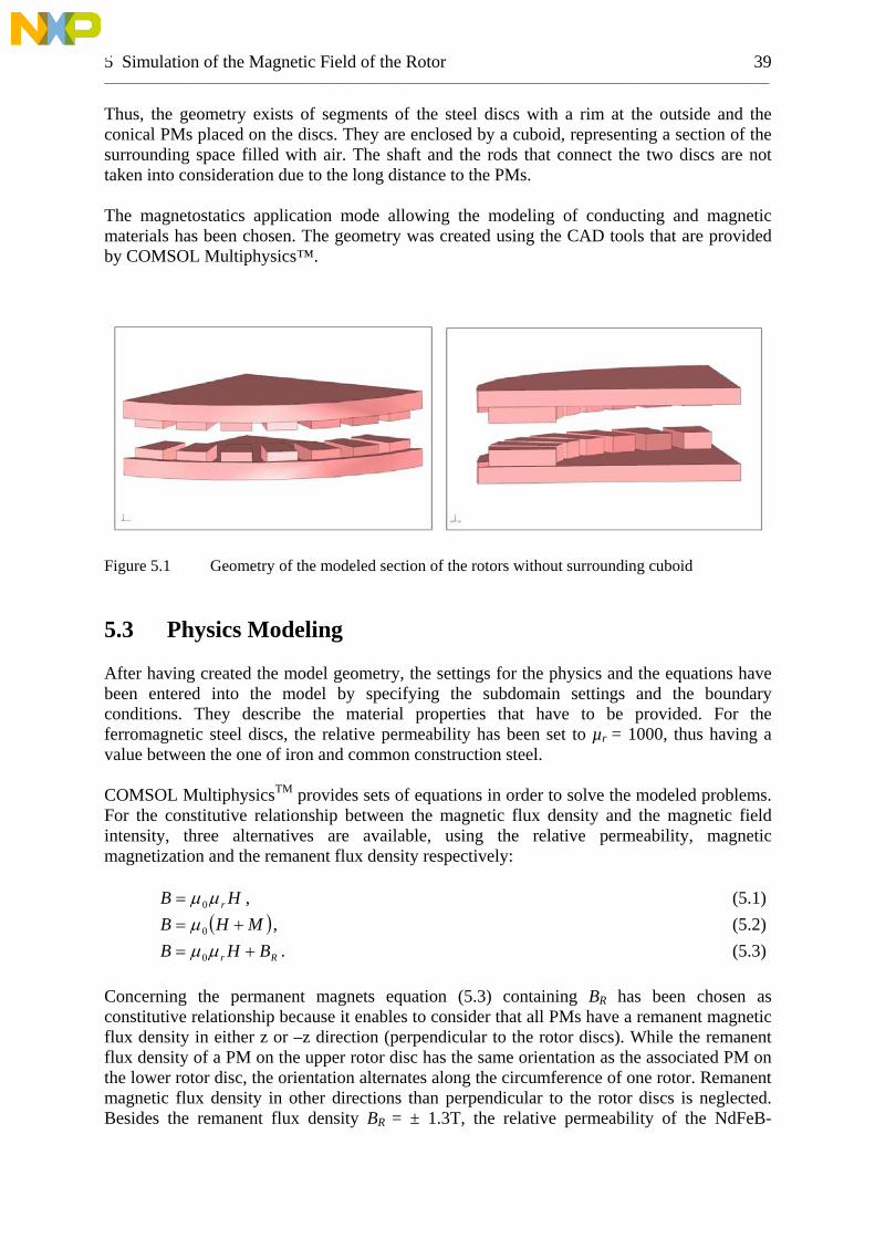
5 Simulation of the Magnetic Field of the Rotor 39 _________________________________________________________________________________________________________________
Thus, the geometry exists of segments of the steel discs with a rim at the outside and the conical PMs placed on the discs. They are enclosed by a cuboid, representing a section of the surrounding space filled with air. The shaft and the rods that connect the two discs are not taken into consideration due to the long distance to the PMs. The magnetostatics application mode allowing the modeling of conducting and magnetic materials has been chosen. The geometry was created using the CAD tools that are provided by COMSOL Multiphysics™.
Figure 5.1 Geometry of the modeled section of the rotors without surrounding cuboid 5.3 Physics Modeling After having created the model geometry, the settings for the physics and the equations have been entered into the model by specifying the subdomain settings and the boundary conditions. They describe the material properties that have to be provided. For the ferromagnetic steel discs, the relative permeability has been set to µr = 1000, thus having a value between the one of iron and common construction steel. COMSOL MultiphysicsTM provides sets of equations in order to solve the modeled problems. For the constitutive relationship between the magnetic flux density and the magnetic field intensity, three alternatives are available, using the relative permeability, magnetic magnetization and the remanent flux density respectively:
HB rμμ0= , (5.1) ( MHB += 0 )μ , (5.2)
Rr BHB += μμ0 . (5.3) Concerning the permanent magnets equation (5.3) containing BBR has been chosen as constitutive relationship because it enables to consider that all PMs have a remanent magnetic flux density in either z or –z direction (perpendicular to the rotor discs). While the remanent flux density of a PM on the upper rotor disc has the same orientation as the associated PM on the lower rotor disc, the orientation alternates along the circumference of one rotor. Remanent magnetic flux density in other directions than perpendicular to the rotor discs is neglected. Besides the remanent flux density BR B = ± 1.3T, the relative permeability of the NdFeB-

5 Simulation of the Magnetic Field of the Rotor 40 _________________________________________________________________________________________________________________
magnets has to be specified for using the equation. According to the manufacturer of the magnets, their relative permeability is µr = 1.05. For the steel disc and the air, equation (5.1) has been chosen. The basis for PDE formulation is Ampére´s law:
JH =×∇ . (5.4) By using the definition of magnetic potential:
AB ×∇= (5.5) and the constitutive equation (5.3), Ampère´s law becomes
( )( ) eRr JBA =−×∇⋅×∇ −− 110 μμ , (5.6)
where eJ : externally generated current density or by using constitutive equation (5.1)
( ) er JA =×∇⋅⋅×∇ −− 110 μμ . (5.7)
5.4 Simulation Results Figure 5.2 a) shows the magnetic flux density along a slice through the middle of the two magnets in the middle of the modeled rotor section. The highest flux density in the middle of the air gap amounts to 0.56 T and the flux density is about 0.5 T in a larger range in the middle of the magnets, the area where the stator is situated when inserted. In Figure 5.2 b) the flux density in the plane parallel to the rotor discs and in the middle of them is shown. Tangential and radial slices are shown in Figure 5.3, giving an impression of the three-dimensional geometry.

5 Simulation of the Magnetic Field of the Rotor 41 _________________________________________________________________________________________________________________
a)
b) Figure 5.2 Magnetic flux density in the air gap (in T)
a) Along a radial slice through the middle of the modeled rotor configuration b) In the plane parallel to and in the middle to the rotor discs
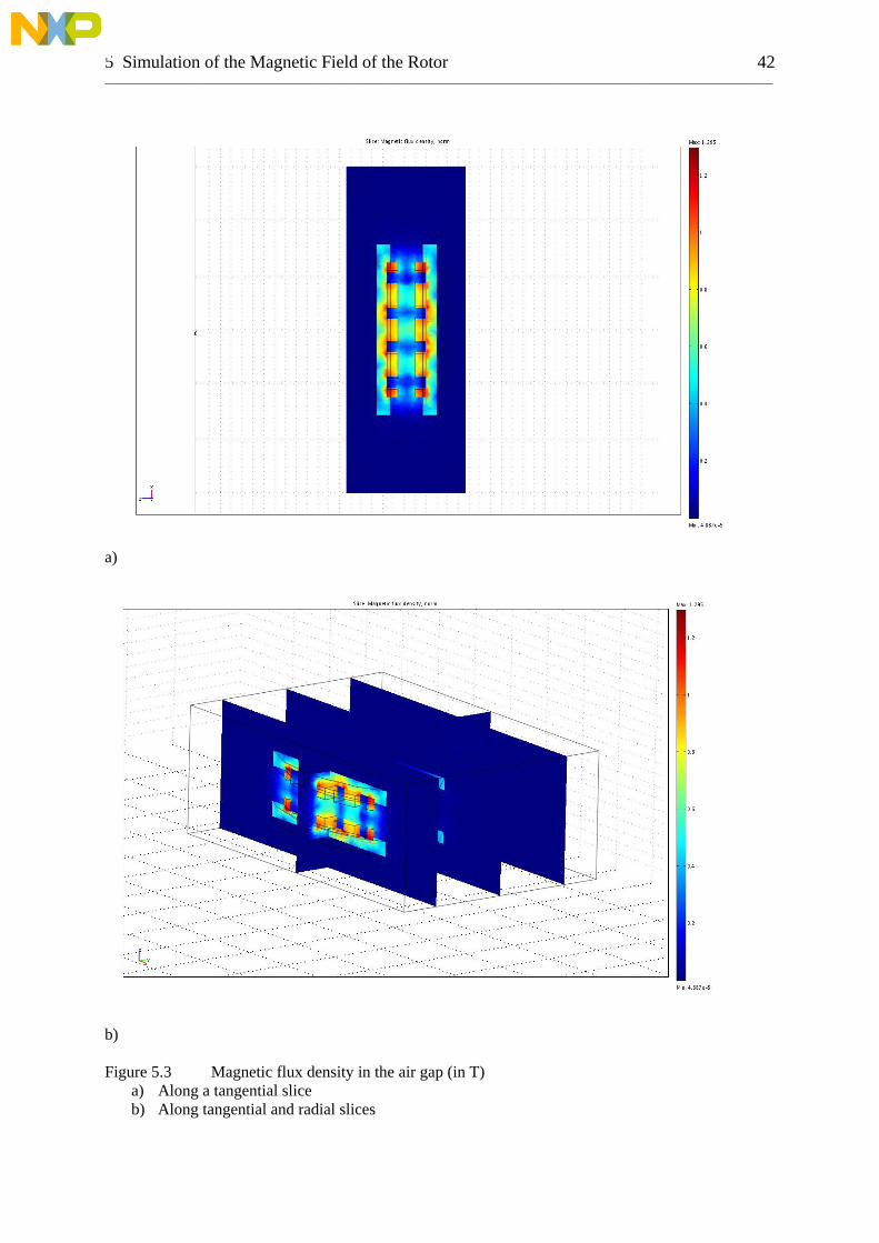
5 Simulation of the Magnetic Field of the Rotor 42 _________________________________________________________________________________________________________________
a)
b) Figure 5.3 Magnetic flux density in the air gap (in T)
a) Along a tangential slice b) Along tangential and radial slices

6 Measurements and Results 43 _________________________________________________________________________________________________________________
6 Measurements and Results 6.1 Measurement of the Magnetic Field of the Rotor By means of a gaussmeter that measures flux density perpendicular to a probe, the flux density of both rotors without inserted stator has been investigated for two different air gaps. Initially, the flux density along a line in radial direction in the middle of the air gap has been measured. The probe was inserted from outside the rotor towards the center of it, following the path shown in Figure 6.2 a). Clearly to perceive, the variation of the flux density is very similar in the 16 mm and 18 mm thick air gaps, but of course higher values of flux density are obtained when the air gap is smaller.
Magnetic field of the rotor
0
100
200
300
400
500
600
-20 -10 0 10 20 30 40 50
Radial position (mm)
Mag
netic
flux
den
sity
(mT)
18 mm air gap16 mm air gap
Figure 6.1 Magnetic flux density in the middle of the air gap, measured from outside to inside
(the radial position zero corresponds to the outer edge of the magnets)
a) radial b) tangential c) axial Figure 6.2 Different directions, in which the probe has been moved for measurements

6 Measurements and Results 44 _________________________________________________________________________________________________________________
The next measurement has been applied in tangential direction over the distance of one pole pitch, again in the middle of the two rotor discs. Despite of the few measurement points, the shape of the curve in Figure 6.3 can be said to be fairly sinusoidal.
-500
-400
-300
-200
-100
0
100
200
300
400
500
0 5 10 15 20 25 30 35
Tangential position (mm)
Mag
netic
flux
den
sity
(mT)
16 mm air gap
Figure 6.3 Variation of the magnetic flux density in tangential direction (measured over one pole
pitch, starting in the middle of a magnet)
0
100
200
300
400
500
600
700
0 1 2 3 4 5 6 7 8 9
Distance from surface of PM (mm)
Mag
netic
flux
den
sity
(mT)
16 mm air gap
Figure 6.4 Variation of the magnetic flux density from the middle of the air gap to the surface of
one of the permanent magnets

6 Measurements and Results 45 _________________________________________________________________________________________________________________
Finally, a measurement was made by moving the probe in axial direction, more exactly towards the magnet above the probe. Figure 6.4 shows how the flux density increases, when the distance to the surface of the magnet is reduced to zero in steps of 1 mm. 6.2 Measurement of the Stator Resistance per Phase By means of a milliohmmeter, the resistance of each phase of the stator winding has been measured to be 134 mΩ. 6.3 Measurement of Phase Voltage at Open-Circuit Operation Figure 6.5 shows the measured voltage of one phase at around 850 rpm, corresponding to an electric frequency of somewhat less than 200 Hz. The amplitude amounts to about 24 V and the shape of the curve is quite sinusoidal. Obviously the content of harmonics is low. The maximum revolution speed that could be reached with the drilling machine was about 900 rpm. If the generator is spinning at this revolution when the drilling machine is removed, it takes about 3 minutes until the revolution speed is reduced to zero due to no-load losses.
Phase voltage
-30
-20
-10
0
10
20
30
-0,006 -0,004 -0,002 0 0,002 0,004 0,006
Time (s)
Volta
ge (V
)
Phase 1
Figure 6.5 Measured open-circuit voltage of one phase 6.4 Connection of a Load A circuit with loads of 1 Ω in each phase was arranged (Y connection). While accelerating the generator, the loads were disconnected. By switching on a circuit breaker, the loads were connected when a rotation speed of approximately 850 rpm was reached. Figure 6.6 shows the voltage drop due to the resistance of the stator winding when the load was connected.
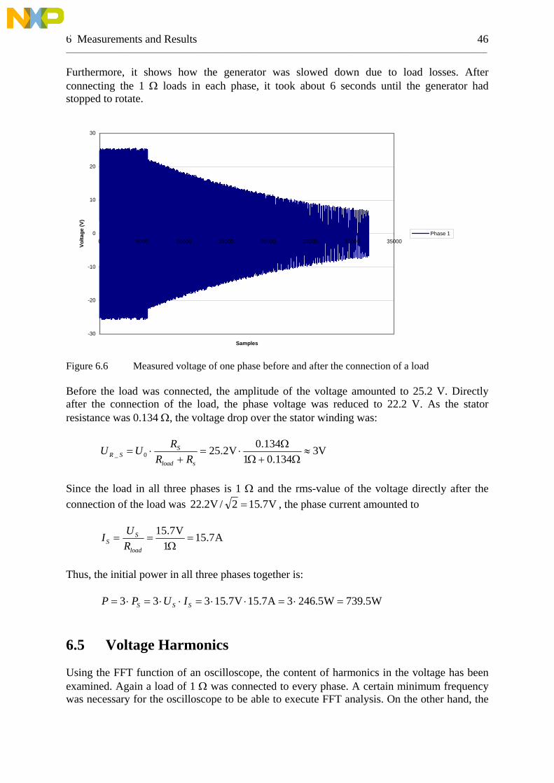
6 Measurements and Results 46 _________________________________________________________________________________________________________________
Furthermore, it shows how the generator was slowed down due to load losses. After connecting the 1 Ω loads in each phase, it took about 6 seconds until the generator had stopped to rotate.
-30
-20
-10
0
10
20
30
0 5000 10000 15000 20000 25000 30000 35000
Samples
Volta
ge (V
)
Phase 1
Figure 6.6 Measured voltage of one phase before and after the connection of a load Before the load was connected, the amplitude of the voltage amounted to 25.2 V. Directly after the connection of the load, the phase voltage was reduced to 22.2 V. As the stator resistance was 0.134 Ω, the voltage drop over the stator winding was:
V3134.01
134.0V2.250_ ≈Ω+Ω
Ω⋅=
+⋅=
sload
SSR RR
RUU
Since the load in all three phases is 1 Ω and the rms-value of the voltage directly after the connection of the load was V7.152/V2.22 = , the phase current amounted to
A7.151
V7.15=
Ω==
load
SS R
UI
Thus, the initial power in all three phases together is:
W5.739W5.2463A7.15V7.15333 =⋅=⋅⋅=⋅⋅=⋅= SSS IUPP 6.5 Voltage Harmonics Using the FFT function of an oscilloscope, the content of harmonics in the voltage has been examined. Again a load of 1 Ω was connected to every phase. A certain minimum frequency was necessary for the oscilloscope to be able to execute FFT analysis. On the other hand, the

6 Measurements and Results 47 _________________________________________________________________________________________________________________
drilling machine has not enough power to accelerate the FW generator to high revolution speeds as long as a load of 1 Ω is connected. Consequently, the range of possible frequencies concerning the fundamental wave was fairly limited. FFT analyses at rotational speeds of about 400 rpm and 500 rpm have been accomplished.
0
0,05
0,1
0,15
0,2
0,25
0,3
0,35
0,4
0,45
0,5
1 3 5 7 9 11 13 15 17 19 21 23 25 27 29 31 33 35 37 39 41 43 45 47 49
Number of harmonic
Frac
tion
of th
e am
plitu
de o
f the
fund
amen
tal w
ave
(%)
408 rpm
Figure 6.7 Content of voltage harmonics at n = 408 rpm
0
0,1
0,2
0,3
0,4
0,5
0,6
0,7
1 3 5 7 9 11 13 15 17 19 21 23 25 27 29 31 33 35 37 39 41 43 45 47 49
Number of harmonic
Frac
tion
of th
e am
plitu
de o
f the
fund
amen
tal w
ave
(%)
522 rpm
Figure 6.8 Content of voltage harmonics at n = 522 rpm

6 Measurements and Results 48 _________________________________________________________________________________________________________________
Figure 6.7 and 6.8 show the content of harmonics as fraction of the amplitude of the fundamental wave. In both cases, the third harmonic is by far the largest one, and the fifth harmonic is the second largest. However, even the amplitude of the third harmonic amounts only to 0.6 percent of the amplitude of the fundamental wave. Generally the total content of harmonics is low, according to these measurements. 6.6 Determination of Losses One of the main purposes of the project was to investigate the losses that occur in the experimental generator. Besides the mechanical losses, the eddy-current and cooper losses in the winding, some other losses may occur. Due to harmonics, the induction of eddy currents in the rotor discs and the permanent magnets is probable. Since it is difficult to determine such losses directly, it was tried to calculate the difference between the total losses and the losses that were easier to determine. This method is applied for example to calculate core losses, which are also difficult to obtain [37]. All appearing losses slow down the generator. When the rotation speed changes, the energy stored in the rotor changes as well. Further on, the reduction of stored energy within a certain time period can be considered as power loss. In addition, the electrical frequency decreases linear with the revolution speed of the generator. The decrease of frequency can be described dependent on the time if the voltage is measured over a certain time. 6.6.1 Standby Losses A spin-down measurement was accomplished. The FW generator was accelerated by a drilling machine to more than 850 rpm. From this time on, when the drilling machine was removed, the rotational speed - and thus the electrical frequency - was decreasing until both were zero. During the time from some seconds before the drilling machine was removed until standstill of the generator the voltage was measured with 10,000 samples per second. As it took about 3 minutes until the rotor had lost its rotational energy, a total of 2,000,000 samples were recorded. The voltage was measured with relatively high resolution over a long period of time. The period time of the voltage was determined by taking the average of some time periods in a short time interval around certain points of time after the removal of the drilling machine. Thus, the frequency could be plotted over the time (see Figure 6.9).

6 Measurements and Results 49 _________________________________________________________________________________________________________________
Frequency over time
0
50
100
150
200
250
0 20 40 60 80 100 120
Time (s)
Freq
uenc
y (H
z)
no load
Figure 6.9 Calculated frequency over time obtained from measurement results As no load was connected to the generator, it was basically slowed down by friction in the bearings and air friction. In addition, the moving magnetic field of the rotor induces eddy currents in the stator cables. As these three losses occur during no-load operation, they can be combined to standby losses. It is assumed that the bearing losses depend linearly on the frequency, whereas the air friction losses and the eddy-current losses in the stator cables increase with the square of the frequency [3]. Equation (6.1) includes the losses increasing with the square of the frequency, which slow down the rotation of the flywheel. In contrast equation (6.2) considers only the losses depending linearly on the frequency.
011 =⋅+⋅=⋅+⋅ ωωωω KJKdtdJ & (6.1)
022 =+⋅=+⋅ KJKdtdJ ωω
& (6.2)
The sum of 6.1 and 6.2 results in:
02 21 =+⋅+⋅⋅ KKJ ωω& (6.3)

6 Measurements and Results 50 _________________________________________________________________________________________________________________
With
JKA 1= (6.4)
and
JKB 2= (6.5)
the equation of motion can be written as:
02 =+⋅+⋅ BA ωω& , (6.6) where A > 0: coefficient describing the part of the losses depending on the square of
the frequency B > 0: coefficient describing the constant part of the losses The solution of this differential equation is given by equation (6.7)
( ) ⎟⎟⎠
⎞⎜⎜⎝
⎛−+⋅=
⋅−⋅−1
AB 2
A2A
0
tteet ωω (6.7)
which is only valid for values of the time t resulting in a frequency ( ) 0≥tω , i.e. for *0 tt ≤≤with
⎟⎟⎠
⎞⎜⎜⎝
⎛⋅+
⋅−=0
* ln2ωAB
BA
t . (6.8)
Equation (6.7) contains two coefficients, A and B, which can be determined by approximating (6.7) to the values obtained from the measured at no load. At the starting time t0 = 0, the value for the starting frequency ω0 amounted to 204.9 Hz (see Figure 6.9). By applying a curve fitting tool and using the measured values of frequency dependent on the time, the coefficients A and B were determined to A = 0.01006 and B = 1.09438. Thus, (6.7) was approximated to the measured values. Figure 6.10 shows the measured frequency compared to the approximated curve, which is almost identical with the points obtained by measurement. That means, the equation (6.7) with the determined coefficients A and B, describes quite well how the frequency depends on the time.

6 Measurements and Results 51 _________________________________________________________________________________________________________________
Frequency over time
0
50
100
150
200
250
0 20 40 60 80 100 120
Time (s)
Freq
uenc
y (H
z)
Frequency frommeasurementApproximationcurve
Figure 6.10 The approximated values of frequency compared to the values obtained by
measurement The power at certain time can be approximated by the change of energy within a short time interval. According to (2.1), the change of energy depends on the change of the angular speed. With (6.7) and the determined values for A and B, the change of energy can be described dependent on the time:
( )( )( )( ) ( )( )
21
22
21
21 21
21
2 tt
tItItPtttP
mm
standby −
⋅⋅−⋅⋅==⎟
⎠⎞
⎜⎝⎛ +=
ωωω . (6.9)
In a next step, a curve is approximated to the values calculated by the means of (6.9). Initially it was assumed that bearing friction losses depend linearly on the frequency and losses due to air friction and eddy-currents losses in the stator cables are proportional to the square of the frequency. Consequently, equation (6.10) should be a suitable equation for being approximated to the values obtained from (6.9), which links frequency to losses.
( ) 221 ωωω ⋅+⋅= AAPstandby (6.10)
Again the curve fitting tool was applied for determining the coefficients, resulting in the values A1 = 0.054 and A2 = 0.0012 respectively. Thus, equation (6.10) was approximated to the values calculated by using (6.9) and (6.7).

6 Measurements and Results 52 _________________________________________________________________________________________________________________
Finally, an expression had been developed, that can be applied for calculating the standby losses depending on the frequency. No information about time was needed anymore. From the curve in Figure 6.11, it can be seen that the losses for high frequencies increase much faster than linearly. If the losses would only rise linearly, the standby losses at 200 Hz would be:
W85.414
Hz2002J054.0211 =
⋅⋅⋅=
⋅⋅⋅=⋅=
ππωp
fAAPlinear .
According to Figure 6.11, standby losses at 200 Hz amount to 14.3 W, i.e. about three times higher than from the bearings.
Figure 6.11 Calculated standby losses dependent on the frequency 6.6.2 Total Losses The same experiment has been accomplished with an electrical load of 1 Ω in each phase (Y connection was applied for the generator and the loads). Again, frequency was determined depending on time, by examining the period time at certain points of time. Figure 6.12 shows the plot of the frequency over time.

6 Measurements and Results 53 _________________________________________________________________________________________________________________
Frequency over time
0
50
100
150
200
250
0 1 2 3 4 5 6
Time (s)
Freq
uenc
y (H
z)
With load
Figure 6.12 Calculated frequency depending on time obtained from measurement results when
operating the flywheel with load The dependence of the frequency on the time has been approximated to the measured values by determining the coefficients f00 and A3 in:
( ) tAtotal eftf ⋅−⋅= 3
00 . (6.11) The coefficients were determined to be A3 = 0.466381 and = 200.8. By using (6.11) and (6.12), the total power losses occurring under load operation can be calculated depending on the time.
00f
( )( )( ) ( )
21
2
2
2
121 14
221
142
21
2 tt
tfItfItfPtttP
mm
totaltotal −
⎟⎠⎞
⎜⎝⎛ ⋅⋅⋅⋅−⎟
⎠⎞
⎜⎝⎛ ⋅⋅⋅⋅
==⎟⎠⎞
⎜⎝⎛ +=
ππ
. (6.12)
In order to obtain an expression, dependent on frequency, an equation containing only ω as variable was needed. Again, linear dependence and dependence on the square of the frequency was presumed. Thus, the equation will look similar to (6.10), but with coefficients A4 and A5 instead of A1 and A2:
( ) 254 AA ωωω ⋅+⋅=totalP . (6.13)
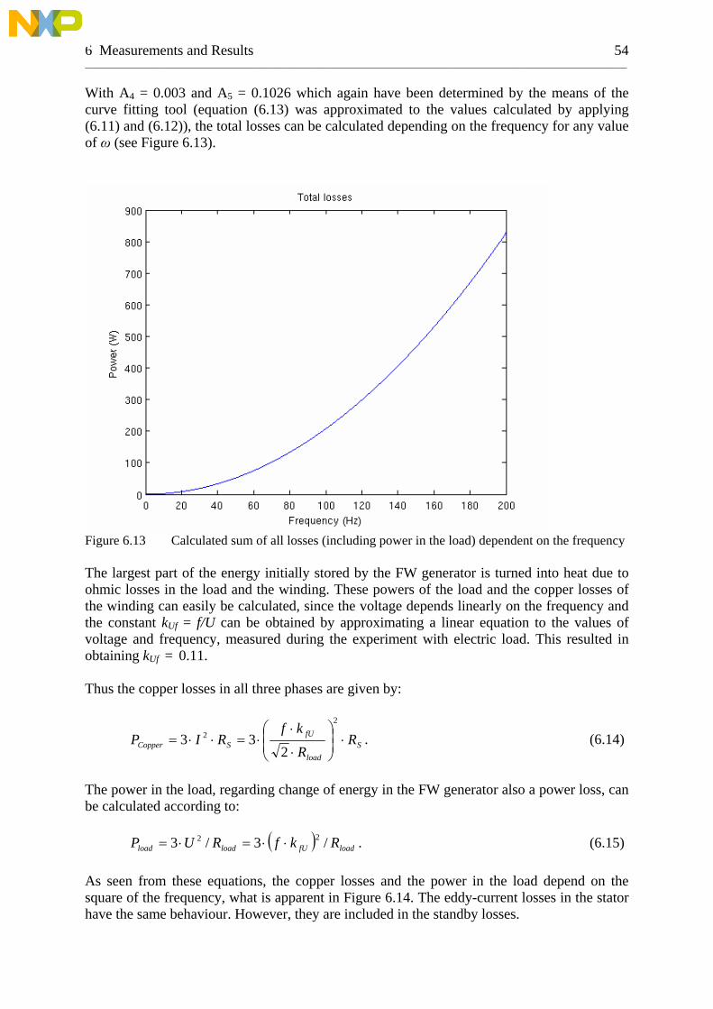
6 Measurements and Results 54 _________________________________________________________________________________________________________________
With A4 = 0.003 and A5 = 0.1026 which again have been determined by the means of the curve fitting tool (equation (6.13) was approximated to the values calculated by applying (6.11) and (6.12)), the total losses can be calculated depending on the frequency for any value of ω (see Figure 6.13).
Figure 6.13 Calculated sum of all losses (including power in the load) dependent on the frequency The largest part of the energy initially stored by the FW generator is turned into heat due to ohmic losses in the load and the winding. These powers of the load and the copper losses of the winding can easily be calculated, since the voltage depends linearly on the frequency and the constant kUf = f/U can be obtained by approximating a linear equation to the values of voltage and frequency, measured during the experiment with electric load. This resulted in obtaining kUf = 0.11. Thus the copper losses in all three phases are given by:
Sload
fUSCopper R
R
kfRIP ⋅⎟
⎟⎠
⎞⎜⎜⎝
⎛
⋅
⋅⋅=⋅⋅=
2
2
233 . (6.14)
The power in the load, regarding change of energy in the FW generator also a power loss, can be calculated according to:
( ) loadfUloadload RkfRUP /3/3 22 ⋅⋅=⋅= . (6.15) As seen from these equations, the copper losses and the power in the load depend on the square of the frequency, what is apparent in Figure 6.14. The eddy-current losses in the stator have the same behaviour. However, they are included in the standby losses.

6 Measurements and Results 55 _________________________________________________________________________________________________________________
a)
b)
Figure 6.14 Measured resistive copper losses and power in the load (voltage over load and resistances of load and resistance of winding have been measured)
a) Resistive copper losses in the stator winding b) The power in the ohmic load over frequency

6 Measurements and Results 56 _________________________________________________________________________________________________________________
The difference between the total losses and the sum of power in the load, copper losses in the winding and the standby losses, might reveal if there were other losses. Figure 6.15 shows Ptotal - Pstandby - Pload - Pcopper.
Figure 6.15 Calculated difference between total losses and sum of standby losses, copper losses in the stator winding and power in load
The sum is negative and amounts to about 1% of the total power losses. Because of inaccuracy of the measurement and arising differences by applying approximation of a curve to a selection of values, the error of this method to determine losses presumably has an error above 1%.
7 Summary of Results and Discussion 57 _________________________________________________________________________________________________________________
7 Summary of Results and Discussion 7.1 Properties of the Experimental Generator 7.1.1 Length of Cable in the Winding Using the measured value for the resistance of the stator, the known cross section area and resistivity of the cable, the cable length per phase in the air-gap winding can be calculated:
m8.18m1078.1
mm5.2134.0 8 =Ω⋅
⋅Ω=⋅= −sqRl
ρ .
2
copper About 3.8 m are used for connection of the stator. Thus, the winding itself comprises about 15 m of cable per phase. 7.1.2 Mechanical Eigenfrequency At revolution speeds between 540 rpm and 570 rpm, the experimental generator vibrates observably. This indicates that the experimental set-up has an eigenfrequency of about 550 Hz and should preferably be operated above this range of revolution speed. 7.1.3 Voltage Harmonics The voltage induced in the winding has a low content of harmonics. The pitched winding and the large air gap reduce the harmonics. The third harmonic has clearly the highest share of the harmonics and the fifth harmonic has the second largest share. This matches the statement, that the content of these both harmonics usually is high for air-gap wound AFPM machines [2]. Table 7.1 shows the winding factors of the air gap winding with q = 2 and 11/12 pitch for the fundamental wave and the harmonics up to ν = 20. The winding factor for the third harmonic, is among the highest. This is in accordance with the results of the FFT measurement.
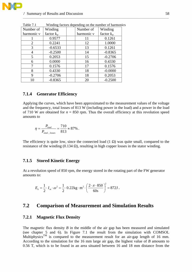
7 Summary of Results and Discussion 58 _________________________________________________________________________________________________________________
Table 7.1 Winding factors depending on the number of harmonics Number of harmonic ν
Winding factor kw
Number of harmonic ν
Winding factor kw
1 0.9577 11 0.1261 2 0.2241 12 1.0000 3 -0.6533 13 0.1261 4 -0.2500 14 -0.8365 5 0.2053 15 -0.2706 6 0.0000 16 0.4330 7 0.1576 17 0.1576 8 0.4330 18 -0.0000 9 -0.2706 18 0.2053 10 -0.8365 20 -0.2500
7.1.4 Generator Efficiency Applying the curves, which have been approximated to the measurement values of the voltage and the frequency, total losses of 813 W (including power in the load) and a power in the load of 710 W are obtained for n = 850 rpm. Thus the overall efficiency at this revolution speed amounts to
%87813710
_
≈==lossestotal
load
PP
η .
The efficiency is quite low, since the connected load (1 Ω) was quite small, compared to the resistance of the winding (0.134 Ω), resulting in high copper losses in the stator winding. 7.1.5 Stored Kinetic Energy At a revolution speed of 850 rpm, the energy stored in the rotating part of the FW generator amounts to:
J872s608502mkg22.0
21
21 2
22 =⎟⎠⎞
⎜⎝⎛ ⋅⋅⋅⋅⋅=⋅⋅=
πωmk IE .
7.2 Comparison of Measurement and Simulation Results 7.2.1 Magnetic Flux Density The magnetic flux density B in the middle of the air gap has been measured and simulated (see chapter 5 and 6). In Figure 7.1 the result from the simulation with COMSOL MultiphysicsTM is compared to the measurement result for an air-gap length of 16 mm. According to the simulation for the 16 mm large air gap, the highest value of B amounts to 0.56 T, which is to be found in an area situated between 16 and 18 mm distance from the

7 Summary of Results and Discussion 59 _________________________________________________________________________________________________________________
outer edge of the magnets. The highest value for B obtained by measurement was 0.509 T, occurring at the positions 14 mm and 16 mm. Thus the highest value obtained by measurement is about 10% lower than the highest value, obtained by simulation. For the most other positions, the measurement results are up to 17% (at positions inside the outer edges of the magnets) lower than the corresponding simulation results. The overall shape of both curves is similar. In Figure 7.2 the results of the simulation and the measurement of the flux density for an air gap length of 18 mm, the size of the actual air gap of the experimental set-up, are compared. Again, the measured values are lower than the one obtained from the simulation. Obviously, the simulation is not very accurate, as the curve of the simulated flux density has quite large steps, and in some regions the flux density increases with decreasing distance from the outer edges of the magnets. The mesh for the simulation with COMSOL MultiphysicsTM was rather coarse, since the calculation complexity of a FEM simulation for solids is high anyway.
0
100
200
300
400
500
600
-10 0 10 20 30 40 50
Radial position (mm)
Flux
den
sity
(mT)
Measurement resultSimulation result
Figure 7.1 Comparison of simulation result and measurement result of the magnetic flux density
in the air gap (16 mm)

7 Summary of Results and Discussion 60 _________________________________________________________________________________________________________________
0
100
200
300
400
500
600
-10 0 10 20 30 40 50
Radial position (mm)
Mag
netic
flux
den
sity
(mT)
Measurement resultSimulation Result
Figure 7.2 Comparison of simulation result and measurement result of the magnetic flux density
in the air gap (18 mm) On the other hand, the results of the measurement might be somewhat lower than the real flux density, as the probe only measures flux density perpendicular to it. Consequently, the measured value becomes too low, if the orientation of the probe is not exactly orthogonal to the flux. Probably there has always been a small angle during the measurement, resulting in reduced values. This means that the actual flux density in the air gap of the rotor configuration has probably values between those obtained by measurement and simulation. A flux density of 0.47 T seems to be a reasonable value. The voltage of the generator operated at 850 rpm can be calculated by applying (3.25) with this value of the flux density:
. This calculated value is fairly close to the measured value of the voltage, suggesting that the assumed value of the flux density is possible.
V1700222Hz850≈⋅⋅⋅⋅⋅⋅⋅⋅
⋅π T47.0m03.m04.96.01460
142
222
^
⋅=
=⋅⋅⋅⋅⋅⋅⋅⋅=Φ⋅⋅⋅
=
π
τπ
πωppwS
wSp BlkNfkNU

7 Summary of Results and Discussion 61 _________________________________________________________________________________________________________________
7.2.2 Voltage Output With the used drilling machine, the generator could be accelerated to a maximum revolution speed of about 900 rpm. At 850 rpm, the measured off-load voltage amounts to Û = 25 V, i.e. the rms-value of the generated voltage is 17.7 V. For the initial simulation with the FEM simulation tool applied for designing the experimental generator, a revolution speed of 2,000 rpm was assumed (see Table 4.1). The generated voltage according to the simulation results was 42 V. Since it was not possible to achieve such a high revolution speed, the simulation was repeated for 850 rpm, resulting in a no-load voltage of U = 14.4 V. This value is about 20% lower than the value obtained by measurement on the experimental set-up. However, both values have the same order of magnitude. 7.3 Discussion of the Measurement and Simulation Results In order to obtain a flux density of 0.47 T in the air gap, a value of 10 mm has to be chosen for the size of the air gap, when doing simulations in the FEM simulation tool. No larger air gap was assumed in the initial simulation, since 10 mm already seemed large compared to the pole pitch of about 3 cm. In Figure 4.4, it is obvious that a large part of the field does not cross the air gap but returns via one of the adjacent permanent magnets. A larger air gap would result in an even smaller portion of field that crosses the air gap and returns via the stator iron. However, as the air-gap wound stator itself is 10 mm thick and some safety margin below and above is applied, the actual air gap of the experimental set-up is 18 mm. In contrast to the stator modeled in the FEM simulation tool, the air-gap wound stator is ironless. Thus, no material with a relative permeability being considerably higher than 1, exists in the air gap. Consequently, the air gap of 18 mm could result in a quite low flux density in the middle of the air gap. On the other hand, there is another magnetic pole on the other side of the air gap. The measurements and calculations show that, by simulating a radial-flux machine with an air gap of 10 mm in the FEM simulation tool, the same flux density is obtained as existing in the 18 mm large air gap of this axial-flux machine with two rotors. First of all, this means that an axial-flux machine can be operated with a large air-gap, as a reasonable flux density still can be achieved. Obviously, the magnetic field is straightened by the PMs of the two rotors. Otherwise a lower fraction of the flux would cross the air gap due to the absence of magnetically conducting material. This statement is supported by the results of the simulation with COMSOL MultiphysicsTM. Figure 5.3 shows that the magnetic flux density between two PMs of the same pole is considerably higher than the flux density between two adjacent PMs. Furthermore, it has been shown that the available FEM simulation tool can be applied as a tool for designing an axial-flux machine, although the value for the air gap used for the simulation differs from the actual air gap. However, it provides only coarse values, which have to be specified by means of other tools.

7 Summary of Results and Discussion 62 _________________________________________________________________________________________________________________
The sum of standby losses, copper losses and the power in the load was slightly larger than the determined total losses, indicating inaccuracy concerning measurement and approximation of equations to the measurement values. This method is obviously not adequate for obtaining information about further losses from the measured data recorded at low revolution speed. However, other losses do obviously not contribute considerably. Had they done so, the difference should be positive and not in the magnitude of the error of measurement. This error is assumed to be reasonably low, since the measurements applied for the determination of losses have been accomplished with high sample rate. It is probable that the eddy-current losses in the PMs and the rotor discs are negligibly small at the low revolution speeds, the generator has been operated on, since these losses increase with the square of the frequency. The low content of harmonics and thus the low occurrence of high frequencies support the assumption that other eddy-current losses than those in the stator winding are very small. To get a considerable contribution of these losses, the generator has to be operated on higher revolution speeds and if possible with smaller air gap in order to increase the content of harmonics in the voltage.

8 Conclusion and Suggestions for Future Work 63 _________________________________________________________________________________________________________________
8 Conclusion and Suggestions for Future Work 8.1 Conclusion A working ironless AFPM air-gap wound generator with cables as stator conductors has been designed and constructed. The resistance of all three phases has the same value RS = 0.134 Ω. At a revolution speed of 850 rpm, an off-load peak voltage of Û = 25 V is generated. A power output of 740 W was achieved by connecting a load of 1 Ω to every phase at a revolution speed of 850 rpm, without any perceivable warming of the cables. Thus, a multiple of this value is achievable by accelerating the generator to higher revolution speed before connecting the load to it. The generated voltage is almost sinusoidal, i.e. its content of harmonics is quite low at the investigated ranges of revolution. The standby losses, i.e. the sum of mechanical losses and eddy-current losses in the stator, and the copper losses have been determined depending on the revolution speed. The contribution of other losses than standby and copper losses could not be determined with the accomplished method. However, it can be assumed that they are very low at the revolution speeds on which the generator has been operated. More accurate measurements at higher revolution speed are necessary in order to determine the eddy-current losses in the PMs and the rotor discs. The simulation results differ up to 20% from the measurement results. Thus, the simulation tools can be applied for roughly designing AFPM generators with air-wound stator. It has been shown that a reasonable high flux density can be obtained, despite a relatively large air gap. The magnets on the two rotor discs straighten the magnetic field compared to a radial flux machine. The generator efficiency of the experimental set-up connected to loads of 1 Ω per phase was about 87% at 850 rpm. 8.2 Suggestions for Future Work A considerably higher contribution of eddy-current losses in the PMs and the rotor discs to the total losses would be achieved by accelerating the experimental FW generator to much higher revolution speeds. The sum of those eddy-current losses could then be determined by applying the same method as in this thesis or by measuring the losses more directly, e.g. by measuring heating of the PMs and the rotor discs. Another way of increasing such losses would be to reduce the air gap if possible without damaging the stator. A smaller air gap would be possible using smaller cables for the air-gap winding or reducing the thickness of the bakelite disc. If a very stiff adhesive could be applied, the disc might be entirely dispensable. While the contribution of the air friction losses to the standby losses could be specified by repeating the spin-down measurement in a vacuum vessel, the contribution of the eddy-

8 Conclusion and Suggestions for Future Work 64 _________________________________________________________________________________________________________________
current losses in the winding could be determined by another spin-down measurement with removed stator. A large reduction of the bearing losses could be achieved by applying magnetic bearings instead of ball bearings. The content of harmonics in the air-gap flux density could be reduced by applying skewed magnets. Connecting a flywheel disc to the generator would increase the stored energy. When accelerating the experimental FW generator to very high revolution speed, the capability of the winding to handle higher voltage could be investigated. Instead of accelerating the set-up mechanically, it could be fed via an IGBT converter and operated as both a motor and a generator, thus becoming an applicable flywheel energy storage, which can absorb, store and supply energy.

9 Acknowledgements 65 _________________________________________________________________________________________________________________
9 Acknowledgements The author would like to thank everybody at the Division for Electricity and Lightning Research at the Uppsala University for their help during my work. A special thank is addressed to my tutor Björn Bolund, to my supervisor Hans Bernhoff and the technician in the tool shop Ulf Ring for assisting with help. Furthermore, I want to thank Csaba Zsolt Deák and Prof. Dr.-Ing. habil. A. Binder at the Institute for Electrical Energy Conversion at the Darmstadt University of Technology for their support.
References 66 _________________________________________________________________________________________________________________
References [1] B. Bolund, H. Bernhoff and M. Leijon, “Flywheel energy and power storage systems”,
Renewable and Sustainable Energy Reviews, 2005. [2] R.-J. Wang, M. J. Kamper, ”Calculation of eddy current loss in axial field permanent-
magnet machine with coreless stator”, IEEE Transactions on Energy Conversion, v 19, n 3, September, 2004, p 532-538
[3] A. Parvianen, “Design of axial-flux permanent-magnet low-speed machines and performance comparison between radial-flux and axial-flux machines”, Thesis for the degree of Doctor of Science, Lappeenranta Univeristy of Technology, Lappeenranta, April 2005
[4] F. Sahin, A.M. Tuckey, A.J.A. Vandenput, “Design, development and testing of a high-speed axial-flux permanent-magnet machine”, Conference Record - IAS Annual Meeting (IEEE Industry Applications Society), v 3, 2001, p 1640-1647
[5] W. Wu, S.B. Dunlop, S.J. Collocott, “Modelling of Eddy-Current Losses in a Surface-Mounted NdFeB Permanent-Magnet Generator”, Proceedings of the Seventeenth International Workshop on Rare-earth Magnets and Applications”, Newark, Delaware, USA, 18-22 August 2002
[6] R. E. Horner and N. J. Proud, “The Key Factors in the design and construction of advanced Flywheel Energy Storage Systems and their application to improve telecommunication power back-up”, in Proc. International Telecommunications Energy Conference, 1996, vol.119, pp. 668-675
[7] http://homepages.cwi.nl/~dik/english/public_transport/odds_and_ends/elec.html, (2006, March)
[8] http://www.travys.ch/Gyrobus.htm, (2006, March) [9] http://www.hansonclan.co.uk/Royal%20Navy/tor_his.htm, (2006, March) [10] http://www.btinternet.com/~philipr/torps.htm, (2006, March) [11] G. Genta, “Shape factor of composite material filament-wound flywheels”,
Composites, Italy, v 12, n 2, Apr, 1981, p 129-134 [12] M. Olszewski, “Advances in flywheel performance for space power applications”,
Endeavour, v 11, n 2, 1987, p 58-62 [13] P. v. Burg, ”Schnelldrehendes Schwungrad aus faserverstärktem Kunststoff”, ETH
Zürich, 1996 (in German) [14] R. Hebner, B. Joseph, A. Walls, ”Flywheel Batteries Come Around Again”, IEEE
Spectrum, 2002, p 46-51 [15] D. Johnson, P. Pillay, M. Malengret, “High speed PM motor with hybrid magnetic
bearing for kinetic energy storage”, Conference Record - IAS Annual Meeting (IEEE Industry Applications Society), v 1, 2001, p 57-63
[16] http://www.railway-energy.org/tfee/index.php?ID=220&TECHNOLOGYID=40&SEL=210&EXPANDALL=3, (2006, March)
[17] http://ureader.de/message/325959.aspx (2006, March) [18] D.A. Christopher, R. Beach, “Flywheel Technology Development Program for
Aerospace Applications”, National Aerospace and Electronics Conference, Proceedings of the IEEE, v 2, 1997, p 602-608
[19] D. Jiles , Introduction to Magnetism and Magnetic Materials, 2nd ed., London: Chapman & Hall, 1998

References 67 _________________________________________________________________________________________________________________
[20] Prof. Dr.-Ing. habil. A. Binder: Script „Elektrische Maschinen und Antriebe 1“, Institut für Elektrische Energiewandlung der Technischen Universität Darmstadt, Darmstadt, 2001 (in German)
[21] http://www.geocities.com/bevs_ei/Alternative_Energy/2_POLE_SYNCHRONOUS_ GENERATOR.gif (2006, March)
[22] http://www.geocities.com/bevs_ei/Alternative_Energy/4_POLE_SYNCHRONOUS_GENERATOR.gif (2006, March)
[23] K.E. Hallenius, Elektriska Maskiner (in Swedish), Malmö: Liber Läromedel, 1972 [24] J. L. Kirtley Jr., Massachusetts Institute of Technology, Department of Electrical
Engineering and Computer Science, 6.685 Electric Machinery, Sept. 2005 http://web.mit.edu/6.685/www/chapter5.pdf , (2006, March)
[25] D. Platt, “Permanent magnet synchronous motor with axial flux geometry”, IEEE Trans Magn, 1989; 25: 3076
[26] F. Profumo, Z. Zhang, A.Tenconi, “Axial Flux Machine Drives: a New Viable Solution for Electric Cars” IECON Proceedings (Industrial Electronics Conference), v 1, 1996, p 34-40
[27] F. Profumo, A. Tenconi, Z. Zhang and A. Cavagnino, “Design and Realization of a Novel Axial Flux Interior PM Synchronous Motor for Wheel-Motors Applications”, Electric Machines and Power Systems, 2000; 28:637-649
[28] S. Nagaya, N. Kashima, H. Kawashima, Y. Kalkiuchi, A. Hoshino, S. Isobe, “Development of the axial gap type motor/generator for flywheel with superconducting magnetic bearings” Physica C: Superconductivity and its Applications, v 392-396 I, n SUPL., October, 2003, p 764-768
[29] M. Aydin, S. Huang, T.A. Lipo, “Axial Flux Permanent Magnet Disc Machines: A Review
[30] R.-J. Wang, J.M. Kamper, K. Van der Westhuizen and J. F. Gieras, ”Optimal Design of a Coreless Stator Axial Flux Permanent-Magnet Generator”, IEEE Transactions on Magnetics, Vol. 41, No. 1, January 2005
[31] H.J. Gray, Dictionary of Physics, London: Longmans, Green and Co Ltd, 1957 [32] W. C. Michels, The International Dictionary of Physics and Electronics, New Jersey:
D. Van Nostrand Company, 1956 [33] R.-J. Wang, M. J. Kamper, ”Evaluation of Eddy Current Losses in Axial Flux
Permanent Magnet (AFPM) Machine with an Ironless Stator”, Conference Record - IAS Annual Meeting (IEEE Industry Applications Society), v 2, 2002, p 1289-1294
[34] M.C. Greaves, G.R. Walker, B.B. Walsh, “Design optimization of Ironless Motors based on Magnet selection”, Journal of Electrical and Electronics Engineering, Australia, v 22, n 1, 2002, p 43-48
[35] Z. Kohari, I. Vajda, Spin-down measurements and loss calculation of multi-layer, multi-pole HTS magnetic bearings, Superconductor Science and Technology, v 18, n 2, February, 2005, p S105-S110
[36] COMSOL Multyphysics, Quick Start And Quick Reference, September 2005 [37] Y. Suzuki, A. Koyanagi, M. Kobayashi, R. Shimada “Novel applications of the
flywheel energy storage system”, Energy, v 30, n 11-12 SPEC. ISS., August/September, 2005, p 2128-2143

Appendix 68 _________________________________________________________________________________________________________________
Appendix A Abbreviations Abbreviation Meaning AFPM Axial flux permanent-magnet emf Electromotive force FEM Finite element method FET Field-effect transistor FES Flywheel energy storage FFT Fast Fourier Transformation FW Flywheel IGBT Insulated-gate bipolar transistor ISS International Space Station LIREX Light Innovative Regional Express mmf Magnetomotive force PDE Partial differential equation PM Permanent magnet rpm Revolutions per minute rms Route mean square SMES Superconducting magnetic energy storage NASA National Aeronautics and Space Administration ISS International Space Station DC Direct current SG Synchronous generator SM Synchronous machine CNC Computerized numeric control NdFeB Neodymium-Iron-Boron SmCo Samarium-cobalt AlNiCo Aluminium-Nickel-Cobalt

Appendix 69 _________________________________________________________________________________________________________________
B Symbols Symbol Quantity Unit a Number of coils connected parallel 1 A area m2
B Magnetic flux density T d Diameter m Ek Kinetic energy J f Electrical frequency Hz F Force N H Magnetic field intensity A/m I Current A Im Polar mass moment of inertia kg·m2
J Current density A/mm2
JM Magnetic polarization T kp Pitch factor 1 kd Distribution factor 1 kw Winding factor 1 K Shape factor 1 l Length m L Inductance H m Mass kg M Magnetization A/m me Number of phases 1 n Revolution speed min-1
Nc Number of turns per coil 1 Ns Number of coil turns per phase 1 p Number of pole pairs 1 P Power W Q Total number of stator slots 1 q Number of slots per pole and phase 1 r Radius m R Resistance Ω U Voltage V w Coil pitch m X Reactance H/s δskin Skin depth m Θ Ampere turns A μ Permeability Vs/Am μr Relative permeability 1 ρ Resistivity Ωm ρm Mass density kg/m3
σ Electrical conductivity S/m σt Tensile strength MPa τα Number of slot steps 1 τp Pole pitch m ν Number of harmonic 1 Φ Magnetic flux Wb

Appendix 70 _________________________________________________________________________________________________________________
χ Susceptibility 1 ω& Angular acceleration rad/s2
ω Angular speed rad/s

Appendix 71 _________________________________________________________________________________________________________________
C Properties of the Sintered NdFeB PM Table A1: Properties of the sintered NdFeB magnets applied for the small-scale generator Property Unit Value Remanence BBR T 1.3 Coercitivity HCB kA/m 875 Intrinsic coercitivity HCJ kA/m 955 Energy product |BH|max kJ/m3 320 Max. working temperature °C 80 Reversible temperature coefficient of BBR (20-100 °C)
%/°C 0.11
Reversible temperature coefficient of HCJ (20-100 °C)
%/°C -0.6
Density g/cm3 7.6 Vickers hardness Hv 570 Tensile strength kg/mm2 8 Specific heat kCal/(kg °C) 0.12 Young´s modulus N/m2 1.6·1011
Poisson´s ratio 0.24 Curie temperature °C 310 Electrical resistivity µΩcm 144 Flexural strength kg/mm 25 Coeff. Of thermal expansion /°C 4·10-6
Thermal Conductivity kCal/(mh°C) 7.7 Rigidity N/m2 0.64 Compressibility m2/N 9.8·10-12
Appendix 72 _________________________________________________________________________________________________________________
D Calculation of Polar Mass Moment of Inertia (m-file) Matlab m-file, used for calculating the polar moment of inertia %% Densities ro_iron = 7.84 * 1000; % kg/m^3 ro_NdFeB = 7.6 * 1000; % kg/m^3 %% Geometry *********************************************** % Rotor r_rotordisc_o = 0.1575; % m r_rotordisc_i = 0.011; % m h_rotordisc = 0.01; % m r_rim_o = 0.1575; % m r_rim_i = 0.150; % m h_rim = 0.003; % m % Shaft r_shaft_upper_part = 0.0055; % m h_shaft_upper_part = 0.06; % m r_shaft_middlepart = 0.011; % m h_shaft_middlepart = 0.095; % m r_shaftring = 0.03; % m h_shaftring = 0.005; % m r_shaft_lower_part = 0.0055; % m h_shaft_lower_part = 0.013; % m % Rod r_rod = 0.0045; % m h_rod = 0.125; % m % Nut r_nut_o = 0.0085; % m r_nut_i = 0.0045; % m % Magnet l_rectangle = 0.04; % m h_rectangle = 0.01; % m b_rectangle = 0.017; % m a_triangel = 0.003 b_triangel = 0; % m c_triangel = 0.04; % m %% Masses ****************************************************** mass_hole = 0.005^2 * pi * 0.01 * ro_iron %kg mass_shaft_upper_part = r_shaft_upper_part^2 * h_shaft_upper_part * pi * ro_iron %kg mass_shaft_middlepart = r_shaft_middlepart^2 * h_shaft_middlepart * pi * ro_iron %kg mass_shaft_lower_part = r_shaft_lower_part^2 * h_shaft_lower_part * pi * ro_iron %kg mass_shaftring = r_shaftring^2 * h_shaftring * pi * ro_iron %kg mass_rotordisc = (r_rotordisc_o^2 - r_rotordisc_i^2)* pi * h_rotordisc * ro_iron - 8 * mass_hole %kg mass_rim = (r_rim_o^2 - r_rim_i^2)* pi * h_rim * ro_iron %kg mass_shaft = mass_shaft_upper_part + mass_shaft_middlepart + mass_shaft_lower_part + mass_shaftring %kg mass_rod = r_rod^2 * pi * h_rod * ro_iron %kg

Appendix 73 _________________________________________________________________________________________________________________
mass_nut = 0.01 %kg mass_magnet = 0.02 * 0.04 * 0.01 * ro_NdFeB %kg mass_rectangle = 0.017 * 0.04 * 0.01 * ro_NdFeB %kg mass_triangel = a_triangel*c_triangel/2*h_rectangle*ro_NdFeB %kg total_mass = 2 * mass_rotordisc + mass_rim + mass_shaft + 4 * mass_rod + 56 * mass_magnet + 20 * mass_nut %kg %% Polar mass moments of inertia % Rotor: I_disc = 0.5 * mass_rotordisc * r_rotordisc_y^2; % kg *m^2 I_rim = 0.5 * mass_rim * (r_rim_o^2 + r_rim_i^2); % kg * m^2 I_rotor = I_disc + I_rim % kg * m^2 % Shaft I_shaft_ovre_del = 0.5 * massa_shaft_ovre_del * r_shaft_ovre_del^2; % kg *m^2 I_shaft_medeldel = 0.5 * massa_shaft_medeldel * r_shaft_medeldel^2; % kg *m^2 I_shaft_nedre_del = 0.5 * massa_shaft_nedre_del * r_shaft_nedre_del^2; % kg *m^2 I_shaftring = 0.5 * mass_shaftring * r_shaftring^2; % kg *m^2 I_shaft = I_shaft_ovre_del + I_shaft_medeldel + I_shaft_nedre_del + I_shaftring % kg * m^2 % Rod I_rod = 0.5 * mass_rod * r_rod^2 + mass_rod * 0.07^2 % kg * m^2 % Nut I_nut = 0.5 * mass_nut * (r_nut_o^2 + r_nut_i^2) + mass_nut * 0.07^2 % kg * m^2 % I_magnet I_rectangle = 1/12 * mass_rectangle * (l_rectangle^2+b_rectangle^2) + mass_rectangle*0.13^2 % kg * m^2 I_triangel = 2*(1/6*a_triangel*c_triangel*c_triangel*c_triangel*massa_triangel + massa_triangel * (0.11 + 0.04*2/3)*(0.11 + 0.04*2/3)) % kg * m^2 I_magnet = I_rectangle + I_triangel % kg * m^2 I_other = 0.5 * 0.02 * 0.02 + 0.02 * 0.07^2 % kg * m^2 % grommets %TOTALT I_total = 2 * I_rotor + I_shaft + 4 * I_rod + 56 * I_magnet + 22 * I_nut % two nuts for welded part
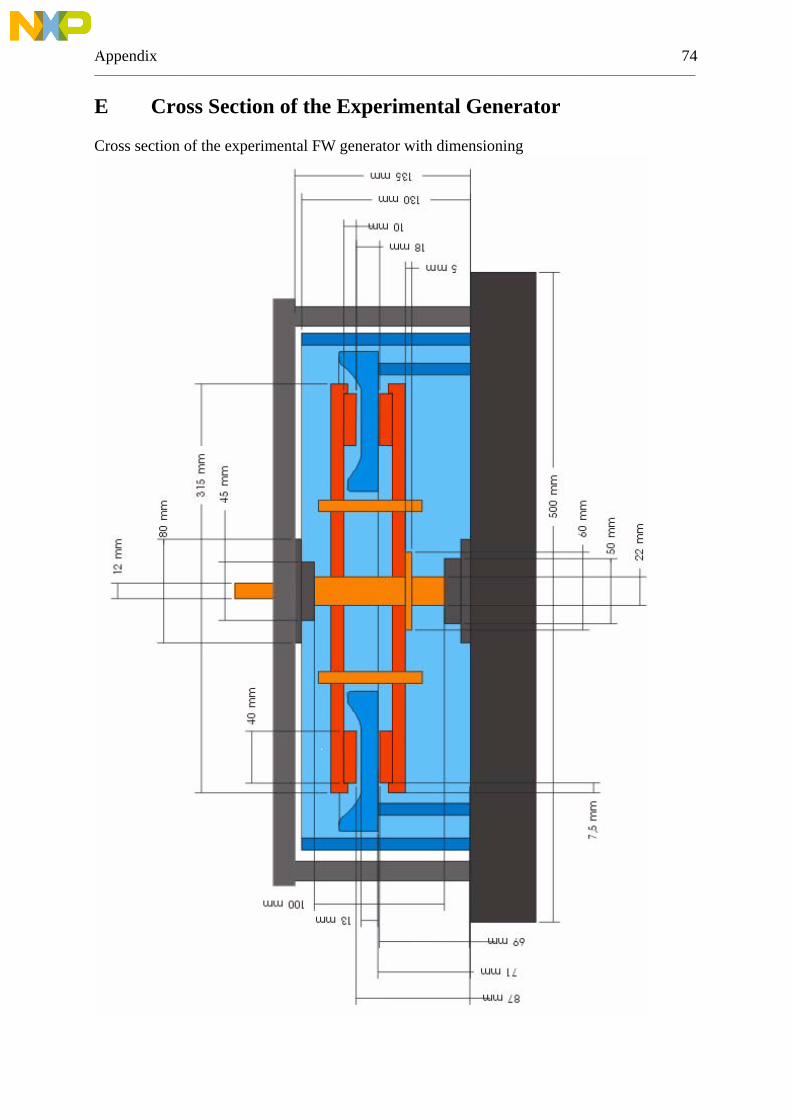
Appendix 74 _________________________________________________________________________________________________________________
E Cross Section of the Experimental Generator Cross section of the experimental FW generator with dimensioning

Appendix 75 _________________________________________________________________________________________________________________
F Pictures of the Experimental FW Generator
Lower rotor disc with PMs Both rotor discs without stator
Both rotor discs with inserted stator Lower rotor disc and stator inside the tube
Completely assembled experimental AFPM generator with air-gap winding

Appendix 76 _________________________________________________________________________________________________________________
G Calculation of Losses of the Experimental Set-Up (m-file) Matlab m-file, used for calculating and plotting the losses dependent on the frequency clear konst_f_U = 0.11 % determined by approximating a curve to the values for f
% and U of the "load measurement" load_resistance = 1.006 % total resistance of load and connecting cable,
% solder and mechanical connections winding_resistance = 0.134 freq = [200.8 188.68 176.06 159.24 148.37 138.12 125.94 112.11 99.6 88.5 78.62 61.88 48.73 37.94 29.45 23.58 18.2 14.04]; %frequencies measured by
%"load measurement" %%%%%%%%%%%%%%%%%%%%%%%with no-load f0=204.9 % value determined by approximating curve f_noload = f0.*exp(-
% A./2.*t)+B./A.*(exp(-A./2.*t)-1) to measured values; A=0.01066 % value determined by approximating curve f_noload = f0.*exp(-
% A./2.*t)+B./A.*(exp(-A./2.*t)-1) to measured values; B=1.094 % value determined by approximating to curve f_noload f0.*exp(-
% A./2.*t)+B./A.*(exp(-A./2.*t)-1) to measured values; I = 0.22 % polar mass moment of inertia t=[0:0.01:200]; f_noload = f0.*exp(-A./2.*t)+B./A.*(exp(-A./2.*t)-1); % freq. at certain
% times plot (t, f_noload); t1 = t - 0.005; % small time intervals t2 = t + 0.005; delta_P1 = 0.5 .*I.*(2.*pi./14).^2 .* ((f0.*exp(-A./2.*t1)+B./A.*(exp(-A./2.*t1)-1)).^2-(f0.*exp(-A./2.*t2)+B./A.*(exp(-A./2.*t2)-1)).^2)./(t2-t1); %Power at certain times %plot (t, delta_P1); %plot (f_noload, delta_P1); a0 = 0.000236342 % value determined by approximating curve P_mech =
% f_noload.*a1 + f_noload.^2.*a0 a1 = 0.0242169 % value determined by approximating curve P_mech =
% f_noload.*a1 + f_noload.^2.*a0
P_mech = f_noload.*a1 + f_noload.^2.*a0; % losses at certain frequency %plot (f_noload, P_mech) %plot (f_noload, P_mech); %%%%%%%%%%%%%%%%%%% with load f00=200.8 % value determined by approximating curve f_load =
% f00.*exp(- a3.*t) to measured values a3 = 0.466381 % value determined by approximating curve f_load =
% f00.*exp(- a3.*t) to measured values f_load = f00.*exp(-a3.*t); % frequency at certain time P_loss = 0.5 .*I.*(2.*pi./14).^2 .*((f00.*exp(-a3.*t1)).^2 - (f00.*exp(- a3.*t2)).^2 )./(t2-t1); %Power at certain times %plot (f_load, P_loss); a4= 0.00135552 % value determined by approximating curve
% P_loss_total = a4.*f_load + a5.*f_load.^2 % to
a5= 0.0206586 % value approximated to curve P_loss_total = % a4.*f_load + a5.*f_load.^2

Appendix 77 _________________________________________________________________________________________________________________
%Figure(8) %P_loss_total = a4.*f_load + a5.*f_load.^2; %plot (f_load, P_loss_total); %%%%%%%%%%%%%%%%%%%%%%%%%%%%%%%%%%%%%%%%%%%%%%%%%%%%%%%%%%%%%%%%%%%%%%%%%%% f = [0:0.01:200]; w2 = 2.*pi.*f; voltage2 = f .* konst_f_U./sqrt(2) % voltage drop over load Figure (1) plot (f, voltage2) title ('Voltage depending on frequency') xlabel ('Frequency (f)') ylabel ('Voltage (V)') p_load2 = 3.*((voltage2).^2)./load_resistance; % power in load Figure (2) plot (f, p_load2) title ('Power in load') xlabel ('Frequency (f)') ylabel ('Power (W)') % copper losses p_winding2 = 3.*(voltage2./(load_resistance)).^2.*winding_resistance; Figure (3) plot (f, p_winding2) title ('Losses in winding') xlabel ('Frequency (f)') ylabel ('Power (W)') p_standby = f.*a1 + f.^2.*a0; % standby losses Figure (4) plot (f, p_standby) title ('Standby losses') xlabel ('Frequency (f)') ylabel ('Power (W)') p_loss_total = a4.*f + a5.*f.^2; % total losses Figure(6) plot (f, p_loss_total) title ('Total losses') xlabel ('Frequency (f)') ylabel ('Power (W)') p_rest = p_loss_total - p_winding2 - p_load2 - p_standby Figure (7) plot (f, p_rest) title ('Difference between total losses and electrical plus mechanical losses') xlabel ('Frequency (f)') ylabel ('Power (W)')