consumption over the life cycle: how different is housing? · consumption over the life cycle: ......

Federal Reserve Bank of MinneapolisResearch Department

Consumption Over the Life Cycle:How Different Is Housing?

Fang Yang∗

Working Paper 635

Revised August 2006

ABSTRACT

Micro data over the life cycle shows two different patterns of consumption of housing and non-housinggoods: the consumption profile of non-housing goods is hump-shaped while the consumption profilefor housing first increases monotonically and then flattens out. These patterns hold true at eachconsumption quartile. This paper develops a quantitative, dynamic general equilibrium model oflife cycle behavior, which generates consumption profiles consistent with the observed data. Bor-rowing constraints are essential in explaining the accumulation of housing assets early in life, whiletransaction costs are crucial in generating the slow downsizing of the housing assets later in life.The bequest motives play a role in determining total life time wealth, but not the housing profile.

Keywords: Consumption, Housing, Life Cycle, Wealth Distribution

JEL Classification: E21, H31, J14, R21

∗Yang, Federal Reserve Bank of Minneapolis and University of Minnesota. I would like to thank MicheleBoldrin, John Boyd, Marco Cagetti, V. V. Chari, Mariacristina De Nardi, Zvi Eckstein, Larry Jones andseminar participants at 2004 CESifo Venice Summer Institute, Federal Reserve Bank at Atlanta, 2005 MidwestMacroeconomics Meetings, 2005 SED meeting, Federal Reserve Bank at Minneapolis, Federal Reserve Bank atChicago, University of Colorado-Boulder, Rutgers University, SUNY-Albany, University of Toronto, IndianaUniversity, Purdue University, Bank of Canada, University of Hong Kong, Hong Kong University of Scienceand Technology, for helpful comments and suggestions. I am grateful to Michele Boldrin and MariacristinaDe Nardi for numerous suggestions and continuous encouragement. Financial support from Gross Fellowshipis gratefully acknowledged. All remaining errors are my own. The views expressed herein are those of theauthor and not necessarily those of the Federal Reserve Bank of Minneapolis or the Federal Reserve System.

1 Introduction

Micro data shows two different patterns of consumption of housing and non-housing goodsover the life cycle. Consumption expenditure of non-housing goods is hump-shaped over thelife cycle: it starts low early in life, rises considerably around middle age, and then falls atmore advanced ages. On the contrary, household holdings of the housing stock are not hump-shaped: lifetime profile of housing stock is monotonically increasing and then rather flat. Thedifferent patterns of housing and non-housing consumption over the life cycle contradict a keyprediction of the standard life cycle model without market frictions: the ratio of housing andnon-housing consumption should not be age-dependent. That is to say, housing consumptionshould follow the same pattern as non-housing consumption.

These stylized facts of life cycle consumption motivate asking which modifications ofthe basic life cycle framework could produce the life cycle consumption profiles that moreclosely resemble the US life cycle consumption profiles. To answer this question, I construct ageneral equilibrium life cycle model of consumption and saving that explicitly models housing.Housing has a dual role: it directly provides utility, and it can be used as collateral. In myframework, households face several frictions: uninsurable labor income risk, lack of annuitymarket to insure against uncertain lifetime, borrowing constraints, and transaction costs fortrading houses. Thus households save to self-insure against labor earning shocks and life-spanrisk, for retirement, to enjoy services from housing, and possibly to leave bequests to theirchildren.

I show that a plausibly parameterized version of my model accounts well for the empiricalfindings. The interaction between housing (which can be used as collateral) and borrowingconstraints leads to the accumulation of housing stock early in life, while transaction coststend to slow the decline of the housing stock later in life. Households begin their economiclives without any housing stock. During the early part of their lives, because of the existenceof borrowing constraints and the role of housing as a collateral, they build housing stockquickly and compromise on non-housing consumption. As households age, they start todecrease their non-housing consumption because their time preference is higher than theinterest rate and mortality rates are increasing along the life cycle. The high transactioncosts associated with trading houses prevent households from decreasing their housing stockquickly later in life.

I also investigate the quantitative relevance of transaction costs, borrowing constraintsand bequest motives in determining this pattern. I find that while borrowing constraintsare essential in explaining the accumulation of housing assets early in life, the existence oftransaction costs is crucial in accounting for the slow downsizing of housing profile laterin life. When choosing a new house, forward-looking households take into account futuretransaction costs. Thus consumption of housing service will be constant at a new leveluntil it is worthwhile to incur the transaction costs again. Thus the home purchase decision

2

is endogenously infrequent. The bequest motives play a role in determining total lifetimewealth, but not housing consumption.

The model is able to capture the life cycle wealth portfolio profiles. In the US, younghouseholds virtually own no liquid financial assets, but hold a major fraction of their wealthas housing. Later in life, households shift their portfolios to financial assets.

The benchmark model also matches the distribution of wealth, housing and financialwealth quite well. It also replicates the empirical finding that inequality in financial assetsis much higher than housing. Households are allowed to borrow against housing so financialassets can be negative but the housing stock can not be. Also the return of housing, marginalutility of housing, is decreasing, while the return to financial assets, the interest rate, isconstant. Thus housing as the fraction of net worth is decreasing.

Understanding the life cycle pattern of consumption and assets allocation behavior iscrucial for policy analysis. Identifying a model capable of explaining the housing and non-housing consumption decisions allows a better understanding of the effect of policy reforms.The house is the single largest expenditure made by consumers over their life time. Themedian household has a house which is valued about twice their annual income. Thus theabstraction from housing may bias the study of life cycle consumption and assets accumula-tion behavior.

The paper is organized as follows. In Section 2, I present some empirical results from theConsumer Expenditure Survey (CEX) and Survey of Consumer Finances (SCF) documentinghouseholds’ consumption and asset accumulation over the life cycle. In Section 3, I presentmy model and define the equilibrium. The calibration of the model is presented in Section 4.Section 5 presents the quantitative results of the benchmark model. Section 6 investigatesthe quantitative importance of the transaction costs, bequest motives, borrowing constraintsand social security. Brief concluding remarks are provided in Section 7. Technical discussionsabout the definition of stationary equilibrium, invariant distribution and bequest distribution,the calibration of aggregate variables and the computational algorithm are provided in theappendix.

1.1 Contribution with respect to the literature

Several mechanisms have been offered in the literature to study the hump-shaped life cycleconsumption profile, such as, precautionary saving and borrowing constraints (Carroll andSummers (1991), Hubbard, Skinner and Zeldes (1994), Carroll (1997), Gourinchas and Parker(2002)), variations in household size (Attanasio and Weber (1995), Attanasio et al. (1999)and Browning and Ejrnæs (2002)), the substitutability of leisure and consumption (Bullardand Feigenbaum (2004)), and mortality risk (Hansen and Imrohoroglu (2005)). None of themincorporate housing. Among the literature that study life cycle consumption profile of durablegoods, Fernandez-Villaverde and Krueger (2002) document that consumption expenditure ishump-shaped over the life cycle and this pattern holds for consumption expenditures on both

3

non-durables and durables, even after controlling for the demographic characteristics of thehouseholds. Fernandez-Villaverde and Krueger (2001) show that a plausibly parameterizedversion of the life cycle model with endogenous borrowing constraints can explain the patternof durable and nondurable consumption expenditure. However, their model cannot generatethe slow decline of the housing stock. Heathcote (2002) incorporates home production in anotherwise standard model to account for the drop of consumption at retirement.

There are several papers that exploit the idea that in the presence of collateralized loans,borrowing constraints distort the intratemporal allocation of resources between durables andnon-durables (see, for example, Brugianini and Weber (1992), Chah et al. (1995), Alessie etal. (1997), Jappelli (1990), and Attanasio et al. (2000)). In contrast to the above literaturethat tests the empirical significance of borrowing constraint from the data, I impose bor-rowing constraints in the model in conjunction with the transaction costs and maintenance-remodeling option.

This paper is related to the strands of optimal portfolio choice in the presence of consumerdurables, such as Grossman and Laroque (1990), Cocco (2000), Flavin and Yamashita (2002),Flavin and Nakagawa (2002), Campbell and Cocco (2003), and Yao and Zhang (2005), andOrtalo-Magne and Rady (2006). In contrast with most models of household portfolio choicethat explicitly include the presence of durables, I model housing in a general equilibriumsetting.

Among the literature on life cycle general equilibrium models that incorporate bequestmotives, De Nardi (2004) constructs a model in which parents and children are linked byaccidental and voluntary bequests and by earning ability and shows that voluntary bequestscan explain the emergence of large estates and the long upper tail of the wealth distribution.I generalize her framework by modeling housing and transaction costs. Ocampo and Yuki(2002) use a similar framework to investigate the quantitative importance of different savingmotives on wealth inequality and aggregate capital accumulation. Laitner (2001) uses anoverlapping generations model with both life cycle saving and altruistic bequest to matchthe high degree of wealth concentration and analyzes the impact of changes in national debtand social security on capital output ratio.

2 Empirical Findings

This section presents my empirical findings on consumption of non-housing and housing overthe life cycle. I first study the life cycle profile of consumption of non-housing goods usingdata from the CEX. I deal explicitly with the changes of household size along the life cycle.Then I look at the life cycle profile of the net worth, housing stock and financial assets derivedfrom the SCF, controlling for cohort and time effects.

The CEX is carried out by the Bureau of Labor Statistics, and is a random samplerotating panel that contains information on demographic characteristics, inventory of major

4

housing and consumption expenditure. The survey consists of a quarterly Interview Surveyin which each consumer unit in the sample is interviewed every three months over a 15-month period, and a Diary Survey which is completed by the sample consumer units for twoconsecutive one-week periods. The Interview Survey is designed to collect data on majoritems of expense, household characteristics, and income. The expenditures covered by thesurvey are those that respondents can recall fairly accurately for three months or longer.The CEX is the only micro-level data set reporting comprehensive measures of consumptionexpenditure for a large cross-section of households in the US.

I use the 2001 CEX data to estimate life cycle profile of non-housing consumption expen-ditures1. I take each household as one observation and use the age of the reference personregardless of the person’s gender. I define 10 cohorts with a length of 5 years, startingfrom age 20. Only households with positive consumption expenditure are selected. Thedata on “expenditure on non-housing consumption” include food, alcoholic beverages, to-bacco, personal care, utilities, household operations, household furnishings and equipment,transportation, books and electronic equipment, apparel, out-of-pocket health expenditure,entertainment and miscellaneous expenditures.

20 30 40 50 60 70 800

0.5

1

1.5

2

2.5

3

3.5

4

x 104 Annual household non−housing consumption (CEX 2001)

15399

29253

17696

mean

Figure 1: Non-housing consumption

Figure 1 plots total household annual expenditure on non-housing goods against the headof the household’s age. Estimated consumption increases from around $15,400 to nearly$29,300, and then decreases to about $17,700. The peak is reached at age forty-five. The sizeof the hump, measured by the ratio of consumption expenditure between the peak and thebeginning of the life cycle, is around 1.9. The consumption expenditure on non-housing goodsdeclines dramatically later in life. The pattern of non-housing consumption is similar to thepattern of nondurable consumption reported in Fernandez-Villaverde and Krueger (2002).

1Fernandez-Villaverde and Krueger (2002) use the CEX data to construct a pseudo panel. They find thatthe results from using pseudo panel and controlling for cohort and time effects is similar to results from usingcross-section data. For simplicity I thus use only the 2001 CEX data.

5

20 30 40 50 60 70 800

0.5

1

1.5

2

2.5

3

3.5

4

4.5


mean1stmedian3rd

Figure 2: Non-housing consumption (quartiles)

If we go beyond mean consumption and look at the distribution of consumption, thehump-shaped non-housing consumption pattern still holds. For example, Figure 2 plots totalhousehold expenditure on non-housing goods at the mean level and at each quartile. Weobserve that the non-housing consumption is hump-shaped at each quartile. We also see thatmean consumption is higher than the median, and lower than the 3rd quartile at each age.This indicates that the distribution of consumption at each age is skewed to the right.

Households of different size plausibly face different marginal utilities from the same con-sumption expenditure. Consequently, changes in household size might explain the hump inconsumption (Attanasio and Weber (1995) and Attanasio et al. (1999)). Thus I adjust thedata for the change in household size along the life cycle using equivalence scales, whichquantify the change in consumption expenditure needed to keep the welfare of families con-stant, regardless of its size (see for example Zeldes (1989), Blundell, Browning and Meghir(1994)). I use the same equivalence scales as Fernandez-Villaverde and Krueger (2002), whichare close to the equivalence scales of the Department of Health and Human Services (FederalRegister (1991)), the estimates of Johnson and Garner (1995) and to the constant-elasticityequivalence scales used by Atkinson et al. (1995), Buhmann et al. (1988) and Johnson andSmeeding (1998), among others. Table 1 shows the equivalence scales I use.

Family Size 1 2 3 4 5

Equivalence scales 1 1.34 1.65 1.97 2.27

Table 1: Equivalence scales

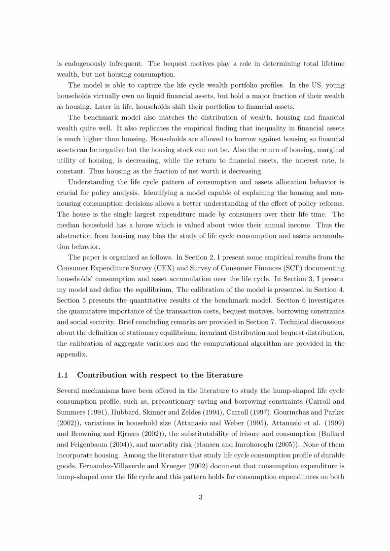
I take non-housing consumption expenditure from the CEX and the demographic infor-mation of the household, and adjust consumption using the above equivalence scales. Figure 3plots the estimated adjusted life cycle profile of adult-equivalent expenditure on non-housinggoods. The adjusted consumption increases from around $12,000 to nearly $18,900 and then

6

decreases to about $14,400. The peak in adjusted consumption is postponed to age fifty-five. The size of the hump, measured by the ratio of consumption expenditure between thepeak and the beginning of the life cycle, is around 1.6. The consumption expenditure onnon-housing goods declines dramatically later in life. We observe that the non-housing con-sumption is hump-shaped at each quartile. We also see that the distribution of consumptionat each age is skewed to the right. The results are robust to using different equivalence scales.

20 30 40 50 60 70 800

0.5

1

1.5

2

2.5


mean1stmedian3rd

Figure 3: Non-housing consumption (adult equivalent)

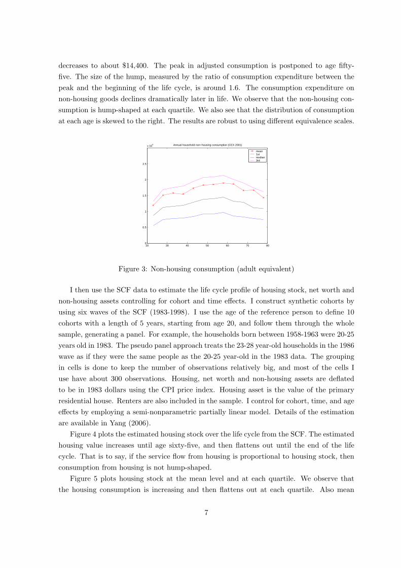
I then use the SCF data to estimate the life cycle profile of housing stock, net worth andnon-housing assets controlling for cohort and time effects. I construct synthetic cohorts byusing six waves of the SCF (1983-1998). I use the age of the reference person to define 10cohorts with a length of 5 years, starting from age 20, and follow them through the wholesample, generating a panel. For example, the households born between 1958-1963 were 20-25years old in 1983. The pseudo panel approach treats the 23-28 year-old households in the 1986wave as if they were the same people as the 20-25 year-old in the 1983 data. The groupingin cells is done to keep the number of observations relatively big, and most of the cells Iuse have about 300 observations. Housing, net worth and non-housing assets are deflatedto be in 1983 dollars using the CPI price index. Housing asset is the value of the primaryresidential house. Renters are also included in the sample. I control for cohort, time, and ageeffects by employing a semi-nonparametric partially linear model. Details of the estimationare available in Yang (2006).

Figure 4 plots the estimated housing stock over the life cycle from the SCF. The estimatedhousing value increases until age sixty-five, and then flattens out until the end of the lifecycle. That is to say, if the service flow from housing is proportional to housing stock, thenconsumption from housing is not hump-shaped.

Figure 5 plots housing stock at the mean level and at each quartile. We observe thatthe housing consumption is increasing and then flattens out at each quartile. Also mean

7

20 30 40 50 60 70 800

1

2

3

4

5

6

7

8

9

10x 10

4 Estimated housing stock from SCF (in 1983 $)

housing

Figure 4: Housing consumption

10 20 30 40 50 60 70 80−2

0

2

4

6

8

10

12x 10

4 Housing Stock

age

mean1st quartilemedian3rd quartile

Figure 5: Housing consumption (quartiles)

consumption is higher than the median at each age, indicating that the distribution of housingconsumption at each age is also skewed to the right.

The finding that elderly households do not decrease their housing consumption is consis-tent with the empirical findings from other literature. For example, Feinstein and McFadden(1989) suggest that more than one-third of elderly households reside in dwellings with at leastthree more rooms than the number of inhabitants, and are thus consuming large housing ser-vices. Fernandez-Villaverde and Krueger (2002) show that, when controlling for time andcohort effects, the peak of (market valued) housing service does not occur until age fifty-five,then decreases slightly, and then flattens out until the end of the life cycle.

To isolate the effect of homeownership on housing assets, I also estimate the profile ofhousing assets, for homeowners only. Figure 6 shows the smoothed age profile of housingassets, for homeowner only, for mean, 1st quartile, median and 3rd quartile. Compared withFigure 5, the profiles for homeowners have similar pattern as the profiles for homeowners and

8

10 20 30 40 50 60 70 800

2

4

6

8

10

12

14x 10

4 Housing Stock

age

mean1st quartilemedian3rd quartile

Figure 6: Housing consumption (owners)

renters together, but the levels are higher. This is simply because Figure 5 are estimatedfrom samples containing renters who don’t have any housing assets.

20 30 40 50 60 70 800

1

2

3

4

5

6

7

US data

Hou

sing

/non

−ho

usin

g co

nsum

ptio

n

Age

per householdper adult equivalent

Figure 7: Ratio of housing to non-housing consumption

Figure 7 plots the ratio of housing to non-housing consumption, when I normalize theratio at age 20 to be 1. This ratio is increasing over the life cycle, reaching 5 (per household)and 7 (per adult equivalent) at age 752.

The different patterns of housing and non-housing consumption over the life cycle thuscontradict to a key prediction of the standard life cycle model without market frictions,age-dependent utility of consumption from housing and non-housing or home production:the ratio of housing and non-housing consumption should not be age-dependent. That is tosay, consumption of housing should follow the same pattern as non-housing consumption.

2I do not adjust family size for housing consumption. Nelson (1988) finds that the economics of scale inshelter is so high that “two can live as cheap as one”.

9

Appendix 8.1 describes the implication of this standard life cycle model in greater detail.

20 30 40 50 60 70 80

0

0.5

1

1.5

2

2.5

3

3.5

4

4.5x 10

5 Wealth composition from SCF (in 1983 $)

wealthhousingfinancial

Figure 8: Age profile of wealth composition

I now show the patterns of wealth accumulation and portfolio composition over the lifecycle. Figure 8 plots mean net worth, housing stock, financial assets against the head of thehousehold’s age. Young agents tend to hold little wealth. Early in life households borrow tobuy houses, and thus save in the form of housing. As time goes by, agents have built stocksof houses and start to increase their holding of financial assets. The profiles of financialassets and housing assets intersect in their early 40’s. Their wealth holding peaks at age 70.However, we do not observe quick decumulation of wealth later in life. Instead, householdscontinue to hold large amount of wealth.

3 The Model

The economy is a discrete-time overlapping generation world with an infinitely-lived govern-ment. The government taxes labor earnings, and provides pensions to the retirees. There areidiosyncratic income shocks. There are no state contingent markets for the household specificshocks. The only financial instrument is a one-period bond. Housing has a dual role: it pro-vides utility as consumption goods, and it can be used as collateral thus the borrowing limitof each household depends on the value of the house. Trading of houses incurs transactioncosts. For simplicity, I assume there is no housing rental market.

3.1 Technology

There is one type of goods produced according to the aggregate production function F (K; L)where K is the aggregate capital stock and L is the aggregate labor input. I assume astandard Cobb-Douglas functional form. The final goods can be either consumed or investedinto physical capital or transformed into housing. Physical capital and housing depreciate atrate δk and δh, respectively. Let H denote the aggregate housing stock in the current period,

10

C the aggregate consumption of non-housing, Ih the aggregate investment on housing, Ik

the aggregate investment on physical capital goods, Tc the total transaction costs for tradinghousing, respectively. The aggregate resource constraint is:

(1) F (K,L) = KαL1−α = C + Ik + Ih + Tc.

Households rent capital and efficient labor units to the representative firm each periodand receive rental income at the interest rate r and wage income at the wage rate w.

3.2 Demographics

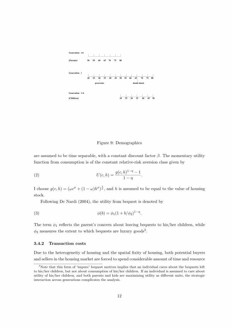
During each model period, which is 5 years long, a continuum of people is born. I denoteage t = 1 as 20 years old, age t = 2 as 25 years old, and so on. At age 20 each person entersinto the model and start working and consuming. Since there are no inter-vivos transfers,all agents start their economic life with no financial assets and no houses. At the beginningof period 3, the agent’s children are born, and four periods later (when the agent is 50 yearsold) the children are 20 and start working. The agents are retired at t = 10 (i.e., when theyare 65 years old) and die for sure by the end of age T = 12 (i.e., before turning 80 yearsold). From t = 10 (i.e., when they are 65 years old), each person faces a positive probabilityof dying given by (1 − pt). The probability of dying is exogenous and independent of otherhousehold characteristics. The population grows at rate n. Since the demographic patternsare stable, agents at age t make up a constant fraction of the population at any point intime. Figure 9 illustrates the demographics in the model.

3.3 Timing and information

At the beginning of each period, households observe their idiosyncratic earning shocks andpossibly receive some inheritance from their parents. Then labor and capital are supplied tofirms and production takes place. Next, the households receive factor payments and maketheir consumption and asset allocation decisions. Housing stocks are not transferred untilthe end of the period. Thus the addition or subtraction to the stock will not influence thepresent period service flow. Finally uncertainty about early death is revealed.

The idiosyncratic labor productivity status is private information and the survival statusis public information. I assume that children can observe their parent’s productivity whentheir parent is 50 and the children are 20.

3.4 Consumer’s maximization problem

3.4.1 Preferences

Individuals derive utility from consumption of non-housing goods, c, from the service flowof the housing, h and from bequests transferred to their children upon death. Preferences

11

Generation t-6

(Parents) 50 55 60 65 70 75 80

Generation t

20 25 30 35 40 45 50 55 60 65 70 75 80

procreate death shock

Generation t+6

(Children) 20 25 30 35 40 45 50

Figure 9: Demographics

are assumed to be time separable, with a constant discount factor β. The momentary utilityfunction from consumption is of the constant relative-risk aversion class given by

(2) U(c, h) =g(c, h)1−η − 1

1− η.

I choose g(c, h) = (ωcσ + (1− ω)hσ)1σ , and h is assumed to be equal to the value of housing

stock.Following De Nardi (2004), the utility from bequest is denoted by

(3) φ(b) = φ1(1 + b/φ2)1−η.

The term φ1 reflects the parent’s concern about leaving bequests to his/her children, whileφ2 measures the extent to which bequests are luxury goods3.

3.4.2 Transaction costs

Due to the heterogeneity of housing and the spatial fixity of housing, both potential buyersand sellers in the housing market are forced to spend considerable amount of time and resource

3Note that this form of ‘impure’ bequest motives implies that an individual cares about the bequests leftto his/her children, but not about consumption of his/her children. If an individual is assumed to care aboututility of his/her children, and both parents and kids are maximizing utility as different units, the strategicinteraction across generations complicates the analysis.

12

to acquire information about the value of a specific housing units. As a consequence, thereare both implicit and explicit search costs associated with moving (Chinloy (1980)). Theseinclude opportunity cost of time associated with market search, brokerage and agent fee,recording fee, legal fee, origination fee. Besides, households have to physically move toa new house, which entail moving costs and psychological costs of breaking neighborhoodattachments (Smith, Rosen, Fallis (1988)).

I consider non-convex transaction costs in the housing stock. A household can buy astock of any size, but once the stock has been bought, it is illiquid. I force the household topay transaction costs every time the household sells and buys a new house. The specificationof the transaction costs is:

(4) τ(h, h′) =

{0 if h′ ∈ [(1− µ1)h, (1 + µ2)h]

ρ1h + ρ2h′ otherwise.

This formulation of transaction costs allow households to change their level of housingconsumption by undertaking housing renovation up to a fraction of µ2 the value of house orby allowing depreciation up to a fraction of µ1 the value of house as an alternative to moving.If the households let the housing depreciate by more that a fraction µ1 of the value, or if thevalue of the stock increases by more that a fraction µ2 of the value, I assume that the stockhas been sold. In those cases, the household has to pay the transaction costs as a fraction ρ1

of its selling value and ρ2 of its buying value.

3.4.3 Borrowing constraints

I assume that only collateralized credit is available and that the borrowing interest rate,mortgage interest rate and deposit interest rate are all equal. This implies that mortgagesand deposits are perfect substitutes. I use at to denote the net asset position. To buy ahouse household must satisfy a minimum down payment requirement as a fraction θ of thevalue of house. Housings also serves as collateral for loans (through home equity loans orrefinancing) up to a fraction (1− θ). At any given period household’s financial assets musthence satisfy:

(5) a′ ≥ −(1− θ)h′,

and household’s net worth is thus always non-negative. Notice in this case, a household’s networth is bounded below by a fraction θ of the value of house4.

4For a household without a house, the borrowing constraint reduces to the standard form a ≥ 0.

13

3.4.4 Labor productivity

In this economy all agents of the same age face the same exogenous age-efficiency profile εt.This profile is estimated from the data and recovers the fact that productive ability changesover the life cycle. Workers also face stochastic shocks to their productivity level. Theseshocks are represented by a Markov process defined on (Y ; B(Y )) and characterized by atransition function Qy, where Y ⊂ R++ and B(Y ) is the Borel algebra on Y . This Markovprocess is the same for all households. This implies that there is no aggregate uncertaintyover the aggregate labor endowment although there is uncertainty at the individual level.The total productivity of a worker of age t is given by the product of the worker’s stochasticproductivity in that period and the worker’s deterministic efficiency index at the same age:ytεt.

To capture the positive correlation in human capital across generations, I assume thatthe parent’s productivity shock at age 50 is transmitted to children at age 20 according to atransition function Qyh, defined on (Y ; B(Y )). What the children inherit is only their firstdraw; from age 20 on, their productivity yt evolves stochastically according to Qy.

For computational reasons, I assume that children cannot observe directly their parent’sassets, but only their parent’s productivity when their parent is 50 and the children are 20,that is, the period when they leave the house and start working5. Based on this information,children infer the size of the bequests they are likely to receive.

3.4.5 The household’s recursive problem

In the stationary equilibrium, the household’s state variables are given by (t, a, h, y, yp), thefirst 4 variables of which denote the agent’s age, financial assets and housing stock carriedfrom the previous period and the agent’s productivity, respectively. The last term yp denotesthe value of the agent’s parent’s productivity at age 50 until the agent inherits and zerothereafter. The law of motion of yp is dictated by the death probability of the parent.When yp is positive, it is used to compute the probability distribution on bequests that thehousehold expects from the parent. When the agents have already inherited, yp is set to be0.

According to the demographic transitions, there are four cases.(i) From t = 1 to t = 3 (from age 20 to 35), the agent survives with certainty until next

period and does not expect to receive a bequest soon because his or her parent is youngerthan 65. For these sub periods yp′ = yp.

(6) V (t, a, h, y, yp) = maxc,a′,h′

{U(c, h) + βE(V (t + 1, a′, h′, y′, yp))

}

5For example, allowing children to observe parents productivity at two periods adds one more state variableand also increases substantially the time needed to iterate over the bequest distributions. Since income in thecalibration is very persistent, an observation of one year of income is likely to be not much less informativethan two.

14

subject to (5) and

c + a′ + h′ + τ(h′, h) = (1− τl)wε + (1 + r)a + (1− δh)h,(7)

c ≥ 0, h′ ≥ 0.(8)

At any subperiod, the agent’s resources are derived from asset holdings, a, labor endow-ment, εty housing stock holding, h. Asset holdings pay a risk-free rate r and labor receives areal wage w. Houses depreciate at rate δh. The evolution of y is described by the transitionfunction Qy. Government taxes labor income at the rate τl.

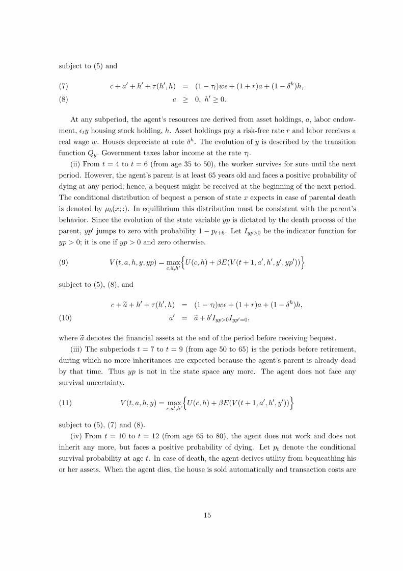
(ii) From t = 4 to t = 6 (from age 35 to 50), the worker survives for sure until the nextperiod. However, the agent’s parent is at least 65 years old and faces a positive probability ofdying at any period; hence, a bequest might be received at the beginning of the next period.The conditional distribution of bequest a person of state x expects in case of parental deathis denoted by µb(x; :). In equilibrium this distribution must be consistent with the parent’sbehavior. Since the evolution of the state variable yp is dictated by the death process of theparent, yp′ jumps to zero with probability 1− pt+6. Let Iyp>0 be the indicator function foryp > 0; it is one if yp > 0 and zero otherwise.

(9) V (t, a, h, y, yp) = maxc,ea,h′

{U(c, h) + βE(V (t + 1, a′, h′, y′, yp′))

}

subject to (5), (8), and

c + a + h′ + τ(h′, h) = (1− τl)wε + (1 + r)a + (1− δh)h,

a′ = a + b′Iyp>0Iyp′=0,(10)

where a denotes the financial assets at the end of the period before receiving bequest.(iii) The subperiods t = 7 to t = 9 (from age 50 to 65) is the periods before retirement,

during which no more inheritances are expected because the agent’s parent is already deadby that time. Thus yp is not in the state space any more. The agent does not face anysurvival uncertainty.

(11) V (t, a, h, y) = maxc,a′,h′

{U(c, h) + βE(V (t + 1, a′, h′, y′))

}

subject to (5), (7) and (8).(iv) From t = 10 to t = 12 (from age 65 to 80), the agent does not work and does not

inherit any more, but faces a positive probability of dying. Let pt denote the conditionalsurvival probability at age t. In case of death, the agent derives utility from bequeathing hisor her assets. When the agent dies, the house is sold automatically and transaction costs are

15

incurred6.

(12) V (t, a, h) = maxc,a′,h′

{U(c, h) + βpt(V (t + 1, a′, h′)) + (1− pt)φ(b)

}

subject to (5), (8) and

c + a′ + h′ + τ(h′, h) = (1 + r)a + (1− δh)h + P,

(13) b = a′ + h′ − τ(h′, 0).

Households receive pension income P. For simplicity, I assume the pension level is inde-pendent of household’s income history7.

4 Calibration

I choose some parameters used in the benchmark model from estimations by other studies.The remaining parameters are chosen so that the model generated data match a given set oftargets. Since one period in my model corresponds to 5 years in real life, I adjust parametersaccordingly.

The rate of population growth, n, is set to the average population growth from 1950 to1997 from Economic Report of the President (1998). The pt’s are the vectors of conditionalsurvival probabilities for people older than 65. I use the mortality probabilities of peopleborn in 1965 provided by Bell, Wade, and Goss (1992).

I construct measures of output Y , capital K and housing H and their investment coun-terparts according to my model. I use data from the National Income and Product Accountsand the Fixed Assets Tables both from the Bureau of Economic Analysis for the year 1954-1999. The aggregate ratios for US economy are calibrated to explicitly consider the existenceof housing that comprises residential assets. Output is defined as measured GDP minushousing services. Capital is defined as the sum of nonresidential private and governmentfixed assets plus the stock of inventories. Investment in capital, I is defined accordingly. Thehousing stock is defined as the stock of private residential assets. Investment in housing, Ih,

is constructed accordingly. The term α is the share of income that goes to capital, whichI turns out to be 0.226. This capital share (non residential stock of capital) is much lowerthan that in other calibrations, which abstract from housing. The rate r is the interest rateon capital net of depreciation. I calibrate δk to be 0.0700 and δh to be 0.0294. Given thecalibration for the US production function, this interest rate is endogenous, and turns out to

6I made this simplification since the children already have houses of their own when they inherit.7A more realistic assumption is that social security benefit is a concave function of the accumulated

contribution. Under this assumption, the accumulated contribution becomes a state variable, which increasesthe computation time dramatically.

16

be 4.37%. Appendix 8.5 explains the rationale behind these choices in greater detail.The deterministic age-profile of the unconditional mean of labor productivity, εt, is taken

from Hansen (1993). Since I impose mandatory retirement at the age of 65, I take εt = 0 fort > 9. The stochastic productivity process is assumed to be an AR(1) process:

ln yt = ρy ln yt−1 + µt µt v N(0, σ2y).

The persistence ρy and variance σ2y are estimated from Panel Study on Income Dynamics

(PSID) data, aggregated over five years in order to be consistent with the model period(Altonji and Villanueva (2002)). The parent’s productivity shock at age 50 is transmitted tochildren at age 20 according to the following transition function:

ln y1 = ρyh ln yh,7 + ν1, ν1 ∼ N(0, σ2yh).

I take ρyh from Zimmerman (1992), and choose σ2yh to match the Gini coefficient of 0.44 for

earnings.The down payment ratio θ is set to be 0.2, which is commonly used in housing literature.

Recently some households are allowed to purchase houses without much initial wealth. How-ever, Caplin et al. (1997) argue that “it is almost impossible for a household to purchase ahome without available liquid assets of at least 10% of the home’s value”. In addition, whatis crucial for my model is the assumption that young and poor household can not borrowbeyond the liquidation value of their collateral. Thus I choose a higher down payment ratiodespite the recent decline of down payment ratio. I see the effect of down payment ratio inSection 6.

Since one of my main interest is to look at how transaction costs affect consumptionand saving decisions, one key calibration is the type of transaction costs that I choose.Smith, Rosen and Fallis (1988) estimate the transaction costs of changing houses, includingsearching, legal costs, cost of readjusting home, and psychological costs from disruption.Their estimation is approximately 8-10 percentage the unit being changed. Martin (2002)finds that the monetary costs of buying a new home, which include agent fee, transfer fee,appraisal and inspection fee, range on average from 7 to 11 percent of purchase price of ahome. Gruber and Martin (2003) estimate the reallocation cost of tax and agency costs fromCEX and find the median household pays costs of the order of 7 percent to sell their housesand 2.5 percent to purchase. In my simulation, I choose transaction costs from sale to beρ1 = 6%, and transaction costs from purchase to be ρ2 = 2%. These values are lower thanthe transaction costs reported above therefore they serve as a lower bound of the effect oftransaction costs. I set µ1 = µ2 = 0. That is to say, if the value of the housing stock increasesor decreases, I assume that the house has been sold.

The social security income P is chosen to be 40% of the average household after taxearnings, a number commonly used in the social security literature. The labor income tax τl

17

is chosen to balance government budget.I take risk aversion parameter, η, to be 1.5, from Attanasio et al. (1999) and Gourinchas

and Parker (2002), who estimate it from consumption data. This value is in the commonlyused range (1-5) in the literature. σ governs the elasticity of substitution between housingand non-housing. Ogaki and Reinhart (1998) use aggregate data and a similar specification,and obtain an estimated σ = 0.145, not significantly different from zero. I thus choose σ tobe 0 so that the momentary utility function g(c, h) takes the Cobb-Douglas form8. I see theeffect of elasticity of substitution between housing and non-housing in Section 6.

I choose the discount factor, β, to match the capital-output ratio. The parameter ω

determines the share of consumption allocated to the non-housing consumption goods andis set to match the ratio of non-housing expenditure to housing stock. I use φ1 to matchbequest output ratio of 2.65% in the US simulation (Gale and Scholz (1994))9. φ2 is chosen tomatch the ratio of average bequest left by single decedents at the lowest 80th percentile overaverage household earnings. According to Hurd and Smith (2001), the average bequest leftby single decedents at the lowest 80th percentile was $125,000 (Asset and Health DynamicsAmong the Oldest Old (AHEAD) data sets, 1993-95).

5 Numerical Results

The benchmark economy allows for housing transaction costs and µ1 = µ2 = 0. That isto say, if the value of the housing stock increases or decreases, I assume that the house hasbeen sold. In this case, the household has to pay the transaction costs as a fraction ρ1 = 6%of its selling value and ρ2 = 2% of its buying value. Some parameters are set so that themodel-generated data match a given set of targets (see Section 4). Appendix 8.6 describesthe computation algorithm in greater detail.

5.1 Life cycle profiles

Now I show the average life cycle profiles of financial assets, total net worth, non-housingconsumption and housing consumption. All figures are normalized by the average householdearnings. These averages are obtained by integrating the policy function with respect tothe equilibrium measure of agents, holding age fixed. For example, the average housingconsumption by an agent at age t is given by

H =∫

h(t, a, h, y, yp)m∗({t} × da× dh× dy × dyp)∫m∗({t} × da× dh× dy × dyp)

Figure 10 compares the average life cycle profiles of annual non-housing consumption and8In this case I add a positive number ε so that utility function is well defined at h = 0. The term ε is small

enough that it does not affect the results. The utility function takes form g(c, h) = cω(h + ε)1−ω

9Since in my model output corresponds to GDP minus housing service, I adjust it accordingly.

18

Parameters Calibrations

Demographics

n population growth 1.2%

pt survival probability see text

Technology

α capital share in National Income 0.226

δk depreciation rate of capital 0.0700

δh depreciation rate of housing 0.0294

Endowment

εt age-efficiency profile see text

ρy AR(1) coefficient of income process 0.85

σ2y innovation of income process 0.30

ρyh AR(1) coefficient of income inheritance process 0.677

σ2yh innovation of income inheritance process 0.37

Government policy

τl social security tax 0.07

P social security replacement rate 0.40

Housing market

θ down payment ratio 0.20

ρ1 transaction costs of selling housing 6%

ρ2 transaction costs of buying housing 2%

µ1 Maximum depreciation 0

µ2 Maximum renovation 0

Preference

η risk aversion coefficient 1.5

σ substitutability of housing and non-housing 0

ω weights of non-housing in utility function 0.8615

β discount factor 0.946

φ1 weight of bequest in utility function −17

φ2 shifter of bequest in utility function 8

Table 2: Parameters used in the benchmark model

19

housing consumption in the model with those in the data reported in Figure 3 and Figure4. I adjust the data so that aggregate non-housing consumption is the same in the dataas in the model10, and aggregate housing stock is the same in the data as in the model.From Figure 10, we see the hump shape of average non-housing consumption, which peaksat age 50’s. The non-housing consumption at age 50 is 80% more than that of age 20, whichis similar to the pattern reported in the data. After the peak, non-housing consumptiondecreases steadily with age. The non-housing consumption at age 50 is 25% more than thatof age 75. Facing an increasing future income profile, young agents would like to borrow tofinance their current consumption but they are borrowing constrained. This explains whyearly in life consumption path increases as income path does. As households age, they startto decrease their non-housing consumption due to the fact that time preference is higher thanthe interest rate and mortality rates are increasing along the life cycle. Compared with data,the non-housing consumption is lower between age 20-35. This may be due to the abstractionof inter-vivos transfers or housing rental market in the model. Inter-vivos transfer relaxesborrowing constraints, while a housing rental market allows young households to have highnon-housing consumption while renting. For detailed discussions of the implications of thosetwo limitations, see Section 7.

20 30 40 50 60 70 800

0.5

1

1.5

2

2.5

3Benchmark Case

Con

sum

ptio

n/av

erag

e ho

useh

old

earn

ings

Age

Non−housing: adult equivalent (data)Housing (data)Non−housing (model)Housing (model)

Figure 10: Life cycle patterns of consumption (benchmark)

The housing consumption profile in the model reproduces the empirically observed in-creasing early in life and slow downsizing later in life. Agents build their housing stock earlyin life and compromise on non-housing consumption. Agents build up their highest housingstock at the age of 60, 5 years later than the peak of non-housing consumption. The elderlydo not decrease their housing stock later in life.

The model also generate the pattern that the ratio of housing to non-housing consumption10In the model I match the aggregate consumption with this in the NIPA. Compared with NIPA, CEX

underreports consumption by a fraction of 30% (see Attanasio, Battistin and Ichimura (2004) for detaileddiscussion). Thus I adjust for the difference accordingly.

20

20 30 40 50 60 70 800

0.5

1

1.5

2

2.5

3

3.5Benchmark Case

Hou

sing

/non

−ho

usin

g co

nsum

ptio

n

Age

datadata (adult equivalent)benchmark modelaggregate h/aggregate c

Figure 11: Ratio of housing to non-housing consumption (benchmark)

increases over the life-cycle. Figure 11 compares this ratio in the model and in the data. Earlyin life, the ratio of housing to non-housing is higher than that in the data. This is becausein the model non-housing consumption is lower than that in the data. Later in life, the ratioof housing to non-housing is lower than that in the data. This is because in the model non-housing consumption is higher than in the data. A parsimonious model without borrowingconstraints and transaction costs in trading houses implies a constant ratio of housing to non-housing consumption, which is equal to H

C . If we denote the difference in the ratio betweenthe data and the parsimonious model without borrowing constraints and transaction costsin trading houses to be 1, the model account for 60% of the difference.

05

1015

2025

−50

0

50

100

1500

5

10

15

20

25

Housing asset

Policy function of housing at 70

Non−housing asset

Figure 12: Policy function of housing stock next period for a 70-year-old

The introduction of transaction costs forces agents to reduce the frequency of transactionsin the housing market. Agents make no change to the stock of the housing unless their non-housing assets and housing stocks are too unbalanced. Two retired agents with the samehousing stock, age and different holding of non-housing assets may choose the same level

21

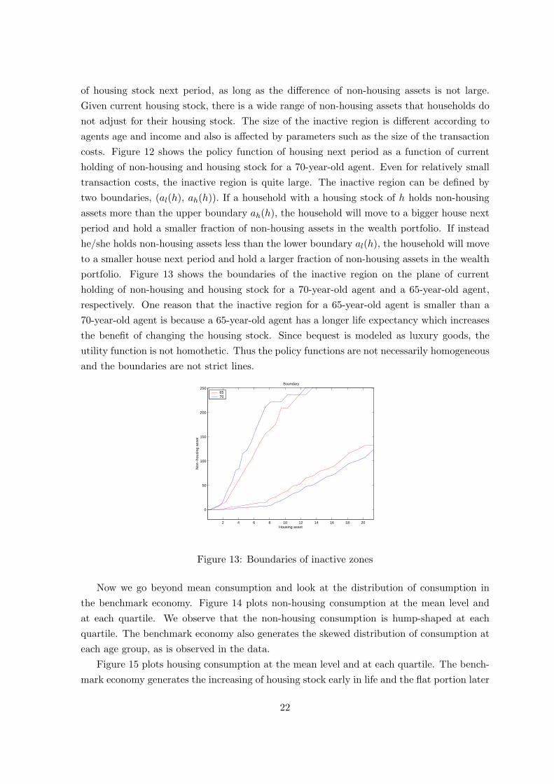
of housing stock next period, as long as the difference of non-housing assets is not large.Given current housing stock, there is a wide range of non-housing assets that households donot adjust for their housing stock. The size of the inactive region is different according toagents age and income and also is affected by parameters such as the size of the transactioncosts. Figure 12 shows the policy function of housing next period as a function of currentholding of non-housing and housing stock for a 70-year-old agent. Even for relatively smalltransaction costs, the inactive region is quite large. The inactive region can be defined bytwo boundaries, (al(h), ah(h)). If a household with a housing stock of h holds non-housingassets more than the upper boundary ah(h), the household will move to a bigger house nextperiod and hold a smaller fraction of non-housing assets in the wealth portfolio. If insteadhe/she holds non-housing assets less than the lower boundary al(h), the household will moveto a smaller house next period and hold a larger fraction of non-housing assets in the wealthportfolio. Figure 13 shows the boundaries of the inactive region on the plane of currentholding of non-housing and housing stock for a 70-year-old agent and a 65-year-old agent,respectively. One reason that the inactive region for a 65-year-old agent is smaller than a70-year-old agent is because a 65-year-old agent has a longer life expectancy which increasesthe benefit of changing the housing stock. Since bequest is modeled as luxury goods, theutility function is not homothetic. Thus the policy functions are not necessarily homogeneousand the boundaries are not strict lines.

2 4 6 8 10 12 14 16 18 20

0

50

100

150

200

250

Housing asset

Non

−ho

usin

g as

set

Boundary

6570

Figure 13: Boundaries of inactive zones

Now we go beyond mean consumption and look at the distribution of consumption inthe benchmark economy. Figure 14 plots non-housing consumption at the mean level andat each quartile. We observe that the non-housing consumption is hump-shaped at eachquartile. The benchmark economy also generates the skewed distribution of consumption ateach age group, as is observed in the data.

Figure 15 plots housing consumption at the mean level and at each quartile. The bench-mark economy generates the increasing of housing stock early in life and the flat portion later

22

20 30 40 50 60 70 800.2

0.4

0.6

0.8

1

1.2

1.4

1.6

1.8

2

Age

Non

−ho

usin

g co

nsum

ptio

n

1st quartilemedian3rd quartilemean

Figure 14: Non-housing consumption (quartiles)

in life at each quartile. The benchmark economy also generates the skewed distribution ofhousing consumption at each age group, as is observed in the data.

20 30 40 50 60 70 800

0.5

1

1.5

2

2.5

3

3.5

Age

Hou

sing

sto

ck

1st quartilemedian3rd quartilemean

Figure 15: Housing consumption (quartiles)

The existence of transaction costs affects young agents and old agents differently. Younghouseholds face increasing income profiles and would like to purchase large houses but theyhave to accumulate enough non-housing assets to pay the down payment. As a result, theyhave to increase their housing stock fairly often. As the households age and their incomeprofile stabilize, households would keep their level of housing stock unchanged, giving thattrading of housing stock would incur transaction costs. Old households are less likely to movethan young household, since they could only consume the new house for a relatively shortperiod of time. Figure 16 shows the fraction of households moving at the end of each periodfor each age group. Moving rates by age in the data is taken from Schachter (2001) and areaggregated to five years. We see moving rates decline with age in the model, as in the data.Moving rates in the data is higher than in the model. One reason is that renters are also

23

20 25 30 35 40 45 50 55 60 65 700

10

20

30

40

50

60

70

80

90

100Moving rates by age (in percent)

Age

ModelData

Figure 16: Moving rates by age

included in calculating the moving rates, and renters tend to move much more frequently thanhomeowners. The other reason is, households move for reasons other than income shocks andaging that this model abstracts from.

20 30 40 50 60 70 80−2

0

2

4

6

8

10

12Benchmark Case

Wea

th/a

vera

ge h

ouse

hold

ear

ning

s

HousingNon−housing assetsNetworth

Figure 17: Life cycle patterns of wealth composition

Figure 17 displays the evolution of wealth portfolio over the life cycle. Young agentstend to hold little wealth. They start with zero wealth and they expect to have much higherearnings in the future. Thus to smooth consumption, they do not hold much wealth. Earlyin life households borrow as much as possible to buy houses, and thus save in the form ofhousing. As time goes by, agents have built stocks of houses and start to increase theirholding of financial assets. The profile of financial assets and housing assets intersect intheir early 40’s, as is observed in the data. The wealth holding peaks at age 65, the yearbefore retirement. After retirement, they start to dissave assets to finance consumption. Oldagents discount their future consumption at a higher rate since the survival probabilities aredeclining in age. This implies that the consumption profile is declining later in life and hence

24

little wealth is needed to finance consumption later in life. Compared with data reportedin Figure 8, the wealth profile and assets profile have humps that are more pronounced.Since I abstract from health expenditure uncertainty or other shocks that could motivateprecautionary assets holding in old age, old agents do not have precautionary saving motivesas they do in the data, therefore they run down their assets more quickly than in the data.

5.2 Wealth distribution

Table 3 reports values for the wealth distribution for my benchmark economy. I presentquintile shares, the 90-95%, the 95-99%, the top 1% shares and Gini coefficient for net worth,housing stocks and financial assets. US wealth distribution is calculated using 1998 SCF. Inthe data wealth is highly unevenly distributed with a Gini coefficient of 0.80. The top 1% ofthe households hold 34% of the total wealth and the 95-99% of the households hold 24% ofthe total wealth. Housing is more evenly distributed than net worth with a Gini coefficientof 0.63. The top 1% of the households hold 11% of the total housing wealth and the 95-99%of the households hold 17% of the total housing wealth. Financial asset is more unevenlydistributed than net worth with a Gini coefficient of 0.99. The top 1% of the households hold46% of the total financial wealth and the 95-99% of the households hold 28% of the totalfinancial wealth11.

The benchmark model matches the distribution of wealth, housing and financial wealthquite well, with the exception of top 1%. It also replicates the empirical finding that inequalityin financial assets is much higher than housing. This is because households are allowed toborrow against housing so financial assets can be negative but the housing stock can notbe. Also for households that are not borrowing constrained, the return of housing, marginalutility of housing, is decreasing, while the return to financial assets, the interest rate, isconstant. Thus housing as the fraction of net worth is decreasing.

5.3 Bequest distribution

Figure 18 compares the cumulative distribution of estate among the whole economy at anygiven time implied by the model with the data. The US data on the estate distributionis from Hurd and Smith (2001) who use the AHEAD data exit interview of 771 deceasedbetween 1993-199512. The size distribution of the bequest is very concentrated both in thedata and in the model: 30% of the deceased AHEAD respondents had an estate of no value13.

11All Gini coefficients are calculated without replacing the negative numbers with zeros. If I replace thenegative numbers with zeros, then the Gini coefficients become slightly smaller

12I use distribution for single decedents. Using the bequest left by singles rather than the one for alldecedents (which turns out to be 1-2 times bigger) is a more sensible choice because typically a survivingspouse inherits a large share of the estate, which will be partly consumed before finally being left to thecouple’s children.

1330% households report leaving no bequest in AHEAD but 70% households report receiving no inheritancein SCF and PSID. One reason is that estates are often divided among several children.

25

Gini 1st 2nd 3rd 4th 5th 90-95 95-99 99-100

Total wealth

U.S. data 0.80 -0.28 1.35 5.14 13.00 81.59 11.48 23.72 33.65

Model 0.74 0.13 0.67 4.04 17.35 77.81 19.91 25.12 10.00

Housing

US data 0.63 0 1.09 13.66 24.10 61.15 13.87 17.12 11.32

Model 0.48 1.73 8.39 14.71 24.59 50.58 13.02 11.79 3.74

Financial wealth

US data 0.99 -6.00 -0.12 1.26 7.23 97.64 11.98 28.20 46.35

Model 0.86 -6.07 -2.68 -0.29 12.32 96.71 24.51 33.70 14.07

Table 3: Wealth distribution

The mean estate was $104,500 but the median was much lower ($62,200). Some respondentsleave relatively large estates: 30% are $120,000 or more and 5% are in excess of $300,000.Only 3% of the estates were valued at $600,000 or more. One parameter of the model ischosen so that the two distributions match at one point: the 80th percentile. The estatedistribution generated by the model actually matches very well to the AHEAD data untilthe 80th percentile of the estate distribution. From that point on, the model predicts largerbequests than those observed in the AHEAD data. The discrepancy is partly due to the factthat AHEAD misses some large estates.

0 20 40 60 80 100 1200.2

0.3

0.4

0.5

0.6

0.7

0.8

0.9

1cumulative distribution of bequest

bequest/average household earnings

modeldata

Figure 18: Cumulative distribution of bequest

Figure 19 shows the bequest distribution for a 35-year-old person conditional on his/herparent’s observed productivity level. At that age, the probabilities of receiving bequests lessthan 2 times output per capita are, respectively, 71%, 19%, 1% and 0%, for people withparents in the lowest, second lowest, second highest and highest productivity levels. Even inthe presence of bequest motives, most of the parents run down their assets after retirement.

26

0 20 40 60 80 100 1200

0.05

0.1

0.15

0.2

0.25

0.3

0.35

0.4

0.45

bequest/average household earnings

lowestsecond lowestsecond highesthighest

Figure 19: Expected bequest distribution at age 35, conditional on parent’s productivity

The fraction of people whose parents live up to the final age of the model economy and whodo not receive a positive bequest are, respectively, 99%, 98%, 88% and 23%, for people withparents in the lowest, second lowest, second highest and highest productivity levels.

6 Decomposition

While the benchmark model does a good job in generating the different patterns of housingand non-housing consumption, and the evolution of assets composition, let us now try tounderstand how each ingredient affects the results. I change one parameter at a time, keepingother parameters as in the benchmark economy. This comparison can shed light on whatrole each feature of the model plays in generating the consumption and assets accumulationprofiles.

First, I change the transaction costs. Then I change the remodeling-maintenance option.I further change parameters that govern the bequest motives. Then I check the effect ofdown payment ratio. I also change the elasticity of substitution between the housing andthe non-housing consumption. Finally I study the effect of the pay-as-you-go social securitysystem.

6.1 Transaction cost

Now I investigate the effects of transaction costs on household consumption and asset hold-ing in this subsection by setting costs to 0. In Figure 20, we see the hump shape of theaverage non-housing consumption, which is similar to the one reported in the data and in thebenchmark model. Compared with the benchmark case, a model without transaction costsgenerates a hump-shaped non-housing consumption profile but the decrease of housing stocklater in life is too fast.

Figure 21 compares the ratio of housing to non-housing consumption in the model with

27

20 30 40 50 60 70 800

0.5

1

1.5

2

2.5

3

Con

sum

ptio

nNon−housing (Benchmark)Housing (Benchmark)Non−housingHousing

Figure 20: Life cycle patterns of consumption (no transaction costs: ρ1 = ρ2 = 0%)

and without transaction costs. Without transaction costs, the ratio becomes flatter over thelife cycle. The ratio is increasing early in life because of the existence of borrowing constraints.Later in life when borrowing constraints are less likely to be binding, a model without trans-action costs implies a flat pattern of the ratio of housing to non-housing consumption. Theseresults show that borrowing constraints are essential in explaining the accumulation of hous-ing assets early in life, while the transaction costs play an important role in explaining theslow decline of housing consumption later in life.

20 30 40 50 60 70 800

0.5

1

1.5

2

2.5

Con

sum

ptio

n ra

tio (

h/c)

BenchmarknoCostaggregate h/c

Figure 21: Ratio of housing to non-housing consumption (no transaction costs: ρ1 = ρ2 = 0%)

Figure 22 shows the average life cycle profiles of financial assets and total net worth. Theevolution of the wealth portfolio over the life cycle is similar to the one in the benchmarkcase. The holding of financial assets is lower than the benchmark. This is because withouttransaction costs, housing assets become more attractive than financial assets. Therefore ahousehold’s portfolio shifts from financial assets to housing assets.

Figure 23 shows the effect of low transaction costs on average non-housing and housingconsumption, when I set ρ1 = 3% and ρ2 = 1%, half as in the benchmark economy. The

28

20 30 40 50 60 70 80−2

0

2

4

6

8

10

12

Wea

lth

Non−housing assets (Benchmark)Networth (Benchmark)Non−housing assetsNetworth

Figure 22: Life cycle patterns of wealth composition (no transaction costs: ρ1 = ρ2 = 0%)

20 30 40 50 60 70 800

0.5

1

1.5

2

2.5

Con

sum

ptio

n

Non−housing (Benchmark)Housing (Benchmark)Non−housingHousing

Figure 23: Life cycle patterns of consump-tion (high transaction costs: ρ1 = 3%,ρ2 = 1% )

20 30 40 50 60 70 80−2

0

2

4

6

8

10

12

Wea

lth


Figure 24: Life cycle patterns of wealthcomposition (high transaction costs: ρ1 =3%, ρ2 = 1% )

housing consumption is higher than that in the benchmark. This is because when transactioncosts are lower, housing assets become more attractive than financial assets. We also seethat when the transaction costs are lower, housing consumption declines slightly after age60. Figure 24 shows that the effect of low transaction costs on net worth profile is small.

Figure 25 shows the effect of high transaction costs on average non-housing and housingconsumption, when I set ρ1 = 8% and ρ2 = 2%. The housing consumption is lower than thatin the benchmark. This is because when transaction costs are higher, housing assets becomeless attractive than financial assets. Figure 26 shows that the effect of high transaction costson net worth profile is small.

6.2 Remodeling-maintenance option

Now I give agents the remodeling-maintenance option. I set µ1 = µ2 = 15% (which is equalto the depreciation rate in 5 years). That is to say, households are allowed to change their

29

20 30 40 50 60 70 800

0.5

1

1.5

2

2.5C

onsu

mpt

ion


Figure 25: Life cycle patterns of consump-tion (high transaction costs: ρ1 = 8%,ρ2 = 2% )

20 30 40 50 60 70 80−2

0

2

4

6

8

10

12

Wea

lth


Figure 26: Life cycle patterns of wealthcomposition (high transaction costs: ρ1 =8%, ρ2 = 2% )

level of housing consumption by allowing depreciation up to 15% the value of the house orby undertaking housing renovation up to a fraction of 15% the value of the house as analternative to moving.

20 30 40 50 60 70 800

0.5

1

1.5

2

2.5

Con

sum

ptio

n


Figure 27: Life cycle patterns of con-sumption (remodeling-maintenance op-tion: µ1 = µ2 = 15%)

20 30 40 50 60 70 80−2

0

2

4

6

8

10

12

Wea

lth


Figure 28: Life cycle patterns of wealthcomposition (remodeling-maintenanceoption: µ1 = µ2 = 15%)

From Figure 27, we see the same hump-shaped non-housing consumption profile. Housingstock is slightly higher than the benchmark model between age 25-35. This shows thatmost households would rather upsize their housing stock a lot therefore the remodeling-maintenance option has little effect. Only when at the last period, we see elderly householdstake the advantage of this option and allow the house to depreciate.

Figure 28 shows the average life cycle profiles of financial assets and total net worth.The evolution of the wealth portfolio over the life cycle is almost identical to the one in thebenchmark case.

30

6.3 Bequest motive

Now I present the results from a model without voluntary bequest motives by setting φ1 = 0.

This modification removes a saving motive thus the aggregate capital stock and outputare lower than in the benchmark economy. Figure 29 compares the average non-housingand housing consumption in the case of no bequest motives and in the benchmark case.Compared with the benchmark case, the profiles of housing and non-housing consumptionhave the similar shape, but the consumption of non-housing goods and housing is lower fromage 45 and on. The reason is households are now receiving accidental bequest, which ismuch smaller than in the benchmark economy with bequest motives, therefore they have lessresources to support consumption after middle age. The bequest motives are not the keyfactor explaining the slow downsizing of housing stock later in life for the average household.The intuition here is that the household faces transaction costs to downsize his/her housingstock, but can run down his/her financial assets without any costs. Without bequest motives,he/she chooses to run down his/her net worth completely by the time he/she expects to bedead for sure. Thus it is optimal to do so by running down his/her financial assets, ratherthan by trading the large house he/she lives in to a smaller one, and thus paying largetransaction costs in the process14.

20 30 40 50 60 70 800

0.5

1

1.5

2

2.5

Con

sum

ptio

n


Figure 29: Life cycle patterns of consump-tion (no bequest motives: φ1=0)

20 30 40 50 60 70 80−2

0

2

4

6

8

10

12

Wea

lth


Figure 30: Life cycle patterns of wealthcomposition (no bequest motives: φ1=0)

Figure 30 compares the average life cycle profiles of financial assets and total net worth inthe case of no bequest motives and in the benchmark case. Compared with the benchmarkcase, the profiles of financial assets and total net worth is much lower from age 45. Thereason is that accidental bequest received is much smaller than in the benchmark economy.The bequest motives, therefore, play an important role in determining total life time wealth

14In the model, mortgages and deposits are perfect substitutes therefore the net mortgage position is inde-terminant. The fact that households run down their financial assets does not necessary mean that householdsare borrowing against their houses using reverse mortgage products. The fraction of households aged 65 andabove who hold wealth more than the value of the house are still pretty high, around 70% in the benchmarkeconomy, and 67% in the case without bequest motive.

31

and financial assets.

20 30 40 50 60 70 800

0.5

1

1.5

2

2.5

Con

sum

ptio

n


Figure 31: Life cycle patterns of consump-tion (high bequest motives: φ1=-22)

20 30 40 50 60 70 80−2

0

2

4

6

8

10

12

14

Wea

lth


Figure 32: Life cycle patterns of wealthcomposition (high bequest motives: φ1=-22)

Since the bequest-output ratio reported in Gale and Scholz (1994) is a low estimate ofthe magnitude of the bequest motives, I present the results from a model with strongervoluntary bequest motives by setting φ1 = −22. A stronger bequest motive increases theaggregate capital stock and output. Figures 31 and 32 show the average life cycle profilesof financial assets and total net worth, non-housing consumption and housing consumption.Compared with the benchmark case, the consumption of non-housing goods and housing ishigher from age 45, the profiles of financial assets and total net worth is much higher fromage 45. The bequest motives, therefore, play an important role in determining total life timewealth and financial assets.

6.4 Down payment

Now I check the effect of the borrowing constraints on consumption paths and wealth pathsby changing down payment ratio. The down payment ratio does affect the consumption ofhousing and non-housing when the households are young. If the down payment ratio is low,then young households are more likely to move into big houses, therefore the housing profileincreases quickly. Figure 33 and Figure 34 show the average life cycle profiles of assets andconsumption paths when the down payment ratio is 0. Compared with the benchmark, theconsumption of housing goods is higher early in life. The profiles of wealth and consumptionare similar to these in the benchmark economy for middle and old households, indicating thatmost of them are not constrained by the down payment requirement. Households use housesas collateral and they have negative financial wealth until their forties, a point at which theybegin to save for retirement. This indicates that saving for purchasing houses is the mainsaving motive for young households.

On the contrary, when the down payment ratio is high, young households have to wait

32

20 30 40 50 60 70 800

0.5

1

1.5

2

2.5C

onsu

mpt

ion


Figure 33: Life cycle patterns of consump-tion (no down payment: θ=0)

20 30 40 50 60 70 80−2

0

2

4

6

8

10

12

Wea

lth


Figure 34: Life cycle patterns of wealthcomposition (no down payment: θ=0)

longer to accumulate more financial assets to pay higher down payments. Figure 35 andFigure 36 show the average life cycle profiles of assets and consumption paths when thedown payment ratio is 0.4. Compared with the benchmark, the consumption of houses islower early in life. Higher down payment ratio implies tighter borrowing constraints, thereforeyoung households could not borrow as much as in the benchmark economy and have higherfinancial assets and higher net worth in this case.

20 30 40 50 60 70 800

0.5

1

1.5

2

2.5

Con

sum

ptio

n


Figure 35: Life cycle patterns of consump-tion (high down payment: θ=0.4)

20 30 40 50 60 70 80−2

0

2

4

6

8

10

12

Wea

lth


Figure 36: Life cycle patterns of wealthcomposition (high down payment: θ=0.4)

6.5 Elasticity of substitution between housing and non-housing consump-

tion

In this subsection we will see the effect of the elasticity of substitution between the housingand non-housing consumption. Figure 37 and Figure 38 compare the average life cycle profilesof assets and consumption paths when the elasticity of substitution between the housing andnon-housing consumption is 0.83 (σ = −0.2) with the benchmark case. We still see the hump-

33

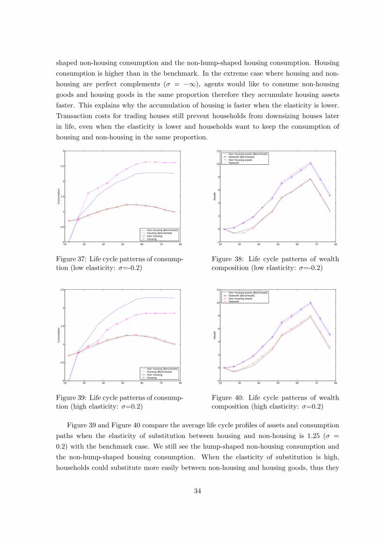
shaped non-housing consumption and the non-hump-shaped housing consumption. Housingconsumption is higher than in the benchmark. In the extreme case where housing and non-housing are perfect complements (σ = −∞), agents would like to consume non-housinggoods and housing goods in the same proportion therefore they accumulate housing assetsfaster. This explains why the accumulation of housing is faster when the elasticity is lower.Transaction costs for trading houses still prevent households from downsizing houses laterin life, even when the elasticity is lower and households want to keep the consumption ofhousing and non-housing in the same proportion.

20 30 40 50 60 70 800

0.5

1

1.5

2

2.5

3

Con

sum

ptio

n


Figure 37: Life cycle patterns of consump-tion (low elasticity: σ=-0.2)

20 30 40 50 60 70 80−2

0

2

4

6

8

10

12

Wea

lth


Figure 38: Life cycle patterns of wealthcomposition (low elasticity: σ=-0.2)

20 30 40 50 60 70 800

0.5

1

1.5

2

2.5

Con

sum

ptio

n


Figure 39: Life cycle patterns of consump-tion (high elasticity: σ=0.2)

20 30 40 50 60 70 80−2

0

2

4

6

8

10

12

Wea

lth


Figure 40: Life cycle patterns of wealthcomposition (high elasticity: σ=0.2)

Figure 39 and Figure 40 compare the average life cycle profiles of assets and consumptionpaths when the elasticity of substitution between housing and non-housing is 1.25 (σ =0.2) with the benchmark case. We still see the hump-shaped non-housing consumption andthe non-hump-shaped housing consumption. When the elasticity of substitution is high,households could substitute more easily between non-housing and housing goods, thus they

34

shift consumption from housing to non-housing. In the extreme case where housing andnon-housing are perfect substitutes (σ = 1), agents will consume non-housing goods but nohousing goods. This is because the net worth is bounded below by fraction θ of the valueof houses, thus a bigger house implies a tighter borrowing constraint. This explains whythe accumulation of housing is slower when the elasticity is high. When the elasticity ofsubstitution is high, households are less willing to pay transaction costs to adjust housingconsumption later in life. Thus transaction costs for trading houses prevent households fromdownsizing houses later in life.

6.6 Pay-as-you-go social security system

Now I look at an economy without a pay-as-you-go social security system. This modificationstrengthens saving for retirement, thus the aggregate capital stock and output are higher thanin the benchmark economy. If I abandon a pay-as-you-go system in which the governmenttaxes working agents and provides social security to retired agents, then young agents are lesslikely to be borrowing constrained, making the average non-housing and housing consumptionincreasing faster early in life. Also abandoning a pension system decreases the hump of wealthprofile. Figure 41 shows the average life cycle profiles of consumption paths. We observethat the shapes of housing and non-housing consumption are similar as in the benchmarkeconomy. The higher level of consumption is caused by the abandonment of social securitytax which leaves agents more resources to consume.

20 30 40 50 60 70 800

0.5

1

1.5

2

2.5

Con

sum

ptio

n


Figure 41: Life cycle patterns of consump-tion (no social security: P=0)

20 30 40 50 60 70 80−2

0

2

4

6

8

10

12

14

16

Wea

lth


Figure 42: Life cycle patterns of wealthcomposition (no social security: P=0)

Figure 42 shows the average life cycle profiles of assets when there is no pay-as-you-gosocial security system. Abandoning a social security system encourages private saving forretirement, thus wealth since the middle age, is much higher than in the benchmark case,and we see much more pronounced humps in wealth and financial asset profiles.

35

7 Conclusions

This paper investigates the degree to which several modifications of the basic life cycle modelproduce consumption profiles of housing and non-housing that more closely resemble featuresof the US. To do this, I develop a quantitative and realistically calibrated dynamic generalequilibrium model to solve numerically for the optimal housing and non-housing consumptiondecisions for a finitely-lived individual who faces several market frictions. One rational forusing dynamic general equilibrium framework is that dynamic general equilibrium modelsare important tools for economic policy evaluation. Furthermore, in this dynamic generalequilibrium framework, the time preference and the interest rate, which greatly affect theintertemporal consumption smoothing and thus the consumption profiles, can be jointlycalibrated without having to match the consumption profiles.

The model is able to match two basic patterns observed in the data: the hump-shapednon-housing consumption profile and non-hump-shaped housing consumption profile. House-holds begin their economic lives without any housing stock. During the early part of theirlives, they are forced to build housing stock and compromise on non-housing consumption.As households age, they start to decrease their non-housing consumption due to the factthat the time preference is higher than the interest rate and mortality rates are increasingalong the life cycle. The high transaction costs for trading houses prevent households fromdecreasing their housing stock quickly later in life.

The model is also able to capture the life cycle wealth portfolio profiles. In the US, younghouseholds virtually own no liquid financial assets, but hold a major fraction of their wealthas housing. Later in life, households shift their portfolios to financial assets.

I also investigate the quantitative relevance of the transaction costs, borrowing constraintsand bequest motives in determining this pattern. I find that while borrowing constraintsare essential in explaining the accumulation of housing assets early in life, the existence oftransaction costs is crucial in explaining the slow downsizing of housing profile later in life.The bequest motives play a role in determining total lifetime wealth, but not the housingprofile.

In this paper I have abstracted from some important issues in order to make the modelmanageable and solvable. Now I discuss these simplifications and their likely quantitativeimplications.

One important assumption is that there are no inter-vivos transfers. In the data, parentstend to give children money when they need money the most, although data from Health andRetirement Study suggests that these transfers are fairly small (see Cardia and Ng (2000)).This assumption is probably relevant when agents are 20 to 35 years of age. Allowing forinter-vivos transfers would make young households have higher housing and non-housingconsumption.

In order to simplify the computation, I do not adopt the literature using endogenous bor-

36

rowing constraints. Fernandez-Villaverde and Krueger (2001) compare the life cycle profilesin a model with endogenous borrowing constraints with the exogenous constraints as in thismodel and they show that the life cycle profiles are identical across these two economies. Themajor difference between the two economies is that with endogenous borrowing constraintsthe net worth of the average young agents is slightly negative, indicating young agents areborrowing to finance the accumulation of housing and to smooth consumption over time andstates. Since I focus on the consumption patterns later in life, I abstract from the endogeneityof borrowing constraints.

Another important assumption that I make is that there is no housing rental market. Inthe Survey of Income and Program Participation (SIPP), housing ownership for two-personhouseholds is low for young households and then increases to 75% at the age of 30, stayingflat and declining only slightly after age 75 (Venti and Wise (2004)). They find that in theabsence of a shock, death of a spouse or entry of a family member into a nursing home,families are unlikely to discontinue home ownership. And even when there is a precipitatingshock, discontinuing ownership is the exception rather than the rule. Thus the rental marketis probably relevant for young households but less relevant for middle and old age households.I could incorporate a rental market into the framework to see if the results presented in thispaper are robust to the existence of a rental market.

I assume that there is no cost of borrowing using housing as collateral. The fixed closingcosts associated with refinancing a mortgage or applying for a second mortgage are estimatedat 1.5 to 2.5 percent of the household’s initial mortgage balance, although accessing homeequity has become much easier in the 1990’s relative to the 1980’s (Bennett, Peach andPeristiani (2001)). Hurst and Stafford (2003) explore the use of equity as a mechanism bywhich households smooth their consumption over time and find that households with lowincome realizations are much more likely to refinance than households with medium or highincome draws. Their analysis assumes households have fixed housing stock and focuses onthe impact of temporary income shocks on refinancing decisions. It will be interesting toextend my model to look at the effect of income shocks on households moving decisions andrefinancing decisions jointly.

I assume that the elderly do no face any health shocks. Even in the presence of socialinsurance (Medicare and Medicaid), households can face substantial out-of-pocket medicalexpenses (see French and Jones (2004), Palumbo(1999) and Feenberg and Skinner(1994)).Moreover nursing home expenses are potentially large and virtually uninsurable (Cohen, Telland Wallack(1986)). The risk of incurring such medical expenses might generate precaution-ary savings and affect the wealth profile (De Nardi, French and Jones(2005)). The effect ofmedical costs on the life cycle consumption and saving in an environment with housing is leftfor future research.

37

8 Appendix

8.1 Consumption ratio in a standard life cycle model

Given budget constraints, a household chooses ct, at+1, ht+1 to maximize its expected lifetimeutility,

maxct,at+1,ht+1

{T∑

t=1

βtE(st−1U(ct, ht) + (1− st)V (ht+1 + at+1))}

subject to

ct + at+1 + ht+1 = yt + (1 + r)at + (1− δh)ht(14)

ct ≥ 0, ht+1 ≥ 0,(15)

where ct is consumption of non-housing assets at age t, at+1 is non-housing assets at age t+1,

ht+1 is housing stock at age t + 1, yt is labor income at age t, which is stochastic, st is theprobability of surviving up to age t, where s0 is 1, r is the interest rate, δh is depreciationrate of housing stock, V is the utility from leaving bequest to their kids, while V = 0 impliesno bequest motives.

Theorem 1: The ratio of consumption of housing to non-housing goods should be age-independent.

Proof of Theorem 1 : Utility maximization implies that the following first order conditionshold:

(16) [ct] : βtst−1U1(ct, ht) = λt

(17) [at+1] : βt(1− st)V ′(at+1 + ht+1) + (1 + r)Etλt+1 = λt

(18) [ht+1] : βt(1− st)V ′(at+1 +ht+1)+βt+1stEtU2(ct+1, ht+1)+ (1− δh)Etλt+1 = λt.

Therefore from equation (17) and (18), we get

(19) βt+1stEtU2(ct+1, ht+1) + (1− δh)Etλt+1 = (1 + r)Etλt+1,

(20) βt+1stEtU2(ct+1, ht+1) = (r + δh)βt+1stEtU1(ct+1, ht+1).

38

Which implies that

(21)EtU2(ct+1, ht+1)EtU1(ct+1, ht+1)

= (r + δh).

After retirement, households do not face income risk so equation (21) takes the deterministicform

(22)U2(ct+1, ht+1)U1(ct+1, ht+1)

= (r + δh).

If we assume

U(c, h) =g(c, h)1−η − 1

1− η(23)

g(c, h) = (ω(c)σ + (1− ω)hσ)1σ ,(24)

then the ratio of housing to non-housing consumption is independent of age t,

(25)(1− ω)hσ−1

ωcσ−1= (r + δh).

That is to say,

(26)h

c= (

(r + δh)ω(1− ω)

)1

σ−1 .

The above model implies that the ratio of consumption of housing to non-housing goodsshould not be age-dependent. The implication of the above model is not consistent with thefacts that later in life consumption of housing is flat while consumption of non-housing goodsis declining.

8.2 Definition of the stationary equilibrium

I focus on an equilibrium concept where factor prices are constant over time and wherecapital and labor are constant in per capita terms. In addition, the age-wealth distributionis stationary over time. Each agent’s state is denoted by x. An equilibrium is described asfollows.

Definition 1 A stationary equilibrium is given by government policies τl, P ; an interestrate r and a wage rate w; value functions V (x), allocations c(x), a′(x), h′(x); a familyof probability distributions for bequests µb(x; :) for a person with state x; and a constantdistribution of people over the state variables x: m∗(x), such that the following conditionshold:

(i) Given the government policies, the interest rate, the wage, and the expected bequest

39

distribution, the functions V (x), c(x), a′(x), and h′(x) solve the above described maximizationproblem for a household with state variables x.

(ii) m∗ is the invariant distribution of households over the state variables for this econ-omy.15

(iii) All markets clear.

K =∫

am∗(dx), H =∫

hm∗(dx), C =∫

cm∗(dx),

L =∫

εym∗(dx), T c =∫

τ(h′, h

)m∗(dx),

F (K; L) = C + (1 + n)K −(1− δk

)K + (1 + n)H − ((1− δh)H − Tc).

(iv) The price of each factor is equal to its marginal product.

r = F1(K, L)− δk, w = F2(K, L).

(v) The family of expected bequest distributions is consistent with the bequests that areactually left by the parents.16

(vi) Government budget is balanced at each period.

8.3 Transition function

From the policy rules and the exogenous Markov process for productivity, we can derive atransition function M(x;·), which is the probability distribution of x′ (the state in the nextperiod), conditional on x, for a person who behaves according to the policy rules c(x), a′(x)and h′(x). Let P be the cardinal set of {1, ..., T} and D indicates that a person is dead, andW = {(a, h) ∈ R× R+ : a ≥ −(1− θ)h}. The measurable space over which M is defined is(X, B(X)), with

X = {1, ..., T} ×W× Y × (Y ∪ {0})B(X) = P({1, ..., T})×B(W)×B(Y )×B(Y ∪ {0})

X = X ∪D

B(X) = {x : x = X ∪ d,X ∈ B(X), d ∈ (φ,D)}),

To characterize M , it is enough to display it for the sets L(t, a, h, y, yp) = {(t′, a′, h′, y′, yp′) ∈15I normalize m∗ so that m∗(X) = 1, which implies that m∗(χ) is the fraction of people alive that are in a

state χ. Appendix 8.3 describes the calculation of invariant distribution in greater detail.16Appendix 8.4 describes the consistency of bequest distribution in greater detail.

40

X : t′ ≤ t, a′ ≤ a, h′ ≤ h, y′ ≤ y, yp′ ≤ yp}. On such sets M is defined by

M(x, L(t, a, h, y, yp))

=

ptIt+1≤tQy(y, [0, y] ∩ Y )Ih′(x)≤h{Ia′(x)≤a(Iyp=0 + Iyp≤yppt+6)

+ µb(x : [0, a− a′(x)](1− pt+6)Iyp>0}, if x 6= D

0, if x = D,

where I is an indicator function, which equals one if the subscript property is true and zerootherwise.

In the above equation, pt is the probability of surviving into the next period. The presenceof It+1≤t shows that conditional on survival, a person currently of age t will be of age t+1 nextperiod. The person’s evolution of productivity is described by Qy. Note that the evolution ofproductivity, a person’s survival, and the survival of the person’s parent are independent ofeach other. If the person’s parent is already dead, that is, yp = 0, the person cannot receivebequests anymore, and his or her assets next period are a′(x) for sure. (As discussed above,this is always the relevant case for people younger than 30 or older than 50.) If, instead,the parent is still alive, that is, yp > 0, the parent can survive into the next period withprobability pt+6. In that case, tomorrow’s assets for the person will be a′(x) and yp′ = yp.Alternatively, the parent may die, with probability 1− pt+6. In this case, the person inheritsnext period, yp′ = 0, and the probability that next period’s assets are no more than a is theprobability of receiving a bequest between 0 and a− a′(x). The last line shows that death isan absorbing state.

In the economy as a whole, I am not interested in keeping track of dead people, so I willdefine an operator on measures on (X, B(X)). Furthermore, I must take into account thatnew people enter the economy in each period. The transition function is defined as

(27) M(x, L(t, a, h, y, yp)) =M(x, L(t, a, h, y, yp)) + n6It=6Qyh(y, [0, y] ∩ Y )Iy=yp′

n.

The transition function M differs from M in two ways. First, it accounts for populationgrowth: when population grows at rate n, a group that is 1% of the population becomes1/(1 + n)% in the subsequent period. Second, it accounts for births, which explains thesecond term in the numerator. If a person is 50 years old (t = 7), that person’s children(there are (1 + n)6 of them) will enter the economy next period. All of those childrenhave age t = 1 and zero assets and zero housing. Their stochastic productivity is inheritedfrom their 50-year-old parents, according to the transition function Qyh. y is their parent’sproductivity at 50.

Let i∗ be the invariant distribution of earnings at age 20 and parent’s earnings at age 50.

41

The invariant distribution is defined recursively as following:

m∗({0} × χ× {0} × {0}) = i∗(χ) ∀χ ∈ B(Y )×B(Y ∪ {0})m∗({0} × χ×W \ {{0} × {0}}) = 0 ∀χ ∈ B(Y )×B(Y ∪ {0})

m∗({t + 1} × χ) =∫

M(x, χ)m∗({t} × dx) ∀t > 1, ∀χ ∈ B(W)×B(Y )×B(Y ∪ {0}).

8.4 Consistency of bequest distributions

I want to calculate the distribution l(·|t, y) of parents at age 50-80, conditional on the parent’sproductivity at age 50 and conditional on being alive. First I define m∗

t,y as the marginaldistribution of x given age t and productivity y as

(28) m∗t,y(χt,y) = m∗(x ∈ X : (t, y) ∈ χt,y) ∀χt,y ∈ P({1, ..., T})×B(Y ).

Next I define m∗(·|t, y) as a probability distribution on (X, B(X)) for any given (t, y). Forany χ ∈ B(X), m∗(·|t, y) is measurable with respect to P({1, ..., T})×B(Y ) and is such that

∫

χt,y

m∗(·|t, y)m∗t,y(dt, dy) = m∗(χ) ∀χ ∈ B(X) ∀χt,y ∈ P({1, ..., T})×B(Y ).

The children observe the parent’s productivity at age 50. Therefore the conditionaldistribution of the parent at age 50 at productivity level yp is m∗(·|t = 7, y = yp). Thereforel(χ|t = 7, y = yp) = m∗(χ|t = 7, y = yp) and recursively using the transition function M

defined in the section above, we define

(29) l(χ|t + 1, yp) =

∫X

M(x, χ)l(dx|t, yp)

pt.

Since the bequest is evenly distributed among children, the probability distributions forbequests µb(x; :) for a person with state x = (t, a, h, y, yp) is given by

µb(x : χ) = l(a ∈ R+, h ∈ R+ : ((1 + n)6a + (1 + n)6(h(1− ρ1)) ∈ χ|t + 6, yp)

∀χ ∈ B(R+), ∀a, h ∈W ∀y, yp ∈ B(Y ).

8.5 Calibration

I calibrate my model following Cooley and Prescott (1995) and Diaz and Luengo-Prado(2003). I use data from the National Income and Product Accounts and the Fixed AssetsTables published by the Bureau of Economic Analysis for the year 1959-2001. In order to

42

properly calibrate a model with two assets and without government taxes and expenditures,I make some imputations.

I define measured GDP as the sum of each final expenditures:

(30) GDP = (c + sh + icd + cg) + (iprk + ipnrk + ig) + nx +4inv,

where c, sh, icd and cg are expenditures on non-housing and service excluding housing,housing services, expenditures on consumer durables, government consumption expenditures,respectively. Thus c + sh + icd + cg are total consumption expenditure. iprk, ipnrk and ig aretotal private residential investment, nonresidential investment and government investment,respectively. Thus iprk + ipnrk + ig are total investment.

I also write GDP as the sum of wages plus rents of residential and nonresidential stocksof capital:

GDP = we + prk · rprk + pnrk · rpnrk.

To explicitly consider the existence of residential housing I rearrange output as

(31) GDP = (c + icd + cg) + sh + iprk + (ipnrk + ig + nx +4inv).

Since there is no rental market in this model, I subtract rental income from residentialhousing from GDP.

Y = we + pnrk · rpnrk = GDP − sh

K = pnrk + inv + g

H = prk

ih = iprk,

where K includes private fixed non-residential assets and government fixed non-residentialassets, H includes private fixed residential assets and government fixed residential assets.Both measures are taken from the Fixed Assets Tables.

Following Cooley and Prescott (1995), I define unambiguous capital income (UCI) asrental income, corporate profits and net interest, and define ambiguous capital income (ACI)as other income excluding wage and depreciation. Thus capital income Yk is defined asUCI+α·ACI+depreciation-sh=α ·Y. Subtracting housing from output, the share of capital iscalibrated as

(32) α = (UCI + dep− sh)/(Y −ACI).

I compute an average share of capital α = 0.2261, an average capital-output ratio KY =

1.9887, an investment-capital ratio ikk = 0.082, a housing stock to output ratio H

Y = 1.2141,

43

an investment-housing stock ratio ihH = 0.041 and a non-housing to housing investment ratio

Cih

= 15.9443. The implied depreciation rates is δk = ikk − n = 0.07, δh = ih

H − n = 0.0294,

interest rate net of depreciation in a steady state is r = α YK − δk = 4.37%.

8.6 Computation of the model

Since I introduce the non-convex transaction costs on housing, I could not use Euler equationapproximation or policy function iteration. Hence I solve the model using approximation ofvalue functions.

To compute the steady state of my model, I first discretize income process and incomeinheritance process following Tauchen and Hussey (1991). The state space for housing andasset holdings are discretized. The upper bounds on the grids are chosen large enough sothat they do not constitute a constraint on the optimization problem. Using these grids Ican store the value functions and the distribution of households as finite-dimensional arrays.

I solve the approximated optimal consumption and saving plans recursively. Householdssurviving to the last period T has an easy problem to solve. Based on the period T policyfunctions, I solve the consumption and saving decisions that maximize the period T − 1value function. The same procedure is carried back until decision rules in the first period arecomputed for a large number of states.

I solve for the steady state equilibrium as follows:1. Given an initial guess of interest rate r, use the equilibrium conditions in the factor

markets to obtain the wage rate w.2. Set the interval for housing and assets.3. Guess an initial bequest distribution.4. Set value function after the last period to be 0 and solve the value function for the

last period of life for each of the points of the grid. This yields policy functions and valuefunction at the last period.

5. By backward induction, repeat step 4 until the first period in life.6. Compute the associated stationary distribution of households by forward induction

using the policy functions starting from the known distribution over types of age.7. Given the stationary distribution and policy functions, compute the bequest distribu-

tion. If the bequest distributions converges, go to step 8; otherwise go to step 3.8. Check if the distributions of housing and assets do not have a large mass at the

maximum levels. If so, increase the maximum level and go back to step 2. If not, continueto step 9.

9. Given the stationary distribution and prices, compute factor input demands andsupplies and check market clearing conditions hold. If all markets clear, an equilibrium isfound. If not, go to step 1 and update interest rate r.

44

References

[1] Alessie, Rob, Michael P. Devereux, and Guglielmo Weber, “Intertemporal Consumption,Durables and Liquidity Constraints: A Cohort Analysis,” European Economic Review,41 (1997), 37-59.

[2] Altonji, Joseph G., and Ernesto Villanueva, “The Effect of Parental Income on Wealthand Bequests,” NBER working paper No. 9811, 2002.

[3] Atkinson, Anthony, Lee Rainwater and Timothy Smeeding, “Income Distribution inOECD Countries: Evidence from the Luxembourg Income Study (LIS),” Social PolicyStudies, 18 (1995), Paris, OECD.

[4] Attanasio, Orazio, James Banks, Costas Meghir and Guglielmo Weber, “Humps andBumps in Lifetime Consumption,” Journal of Business and Economics, 17 (1999), 22-35.

[5] ———–, Erich Battistin and Hidehiko Ichimura, “What Really Happened to Consump-tion Inequality in the US?” NBER Working Paper No. 10338, 2004.

[6] ———–, Pinelopi K. Goldberg and Ekaterini Kyriazidou, “Credit Constraints in theMarket for Consumer Durables: Evidence from Micro Data on Car Loans,” NBERWorking Paper No. 7694, 2000.

[7] ———– and Guglielmo Weber, “Is Consumption Growth Consistent with IntertemporalOptimization? Evidence for the Consumer Expenditure Survey,” Journal of PoliticalEconomy 103 (1995), 1121-1157.

[8] Beaulieu, Joseph J., “Optimal Durable and Nondurable Consumption with TransactionsCosts,” Federal Reserve Board Finance and Economics Discussion Series, April 1993.

[9] Bell, Felicitie C., Alice H. Wade and Stephen C. Goss, “Life Tables for the United StatesSocial Security Area 1900-2080,” Actuarial Study No. 107, US Department of Health andHuman Services, Social Security Administration, Office of the Actuary, August 1992.

[10] Bennett, Paul, Richard Peach and Stavros Peristiani, “Structural Changing in the Mort-gage Market and the Propensity to Refinance,” Journal of Money, Credit and Banking,33 (2001), 955-75.

[11] Blundell, Richard, Martin Browning and Costas Meghir, “Consumer Demand and theLife-Cycle Allocation of Household Expenditures,” Review of Economic Studies, 61(1994), 57-80.

[12] Browning, Martin, and Mette Ejrnæs, “Consumption and Children,” Centre for AppliedMicroeconometrics Working Paper, 2002.

45

[13] Brugiavini, Agar, and Guglielmo Weber, “Durable and Nondurable Consumption: Evi-dence from Italian Household Data,” IFS Working Paper 92/13, 1992.

[14] Buhmann, Brigitte, Lee Rainwater, Guenther Schmaus, and Timothy M. Smeeding,“Equivalence Scales, Well-Being, Inequality and Poverty: Sensitivity Estimates acrossTen Countries Using the Luxembourg Income Study Database,” Review of Income andWealth, 34 (1988), 115-142.

[15] Bullard, James and James Feigenbaum, “A Leisurely Reading of the Lifecycle Consump-tion Data,” Working Paper, 2004.

[16] Campbell, John Y., and Joao F. Cocco, “Household Risk Management and OptimalMortgage Choice,” Quarterly Journal of Economics, 118 (2003), 1149-1194.

[17] Caplin, Andrew, Sewin Chan, Charles Freeman and Joseph Tracy, Housing Partnerships:A New Approach to a Market at a Crossroads (Cambridge: MIT Press, 1997).

[18] Cardia, Emanuela, and Serena Ng, “How Important are Intergenerational Transfers ofTime? A Macroeconomic Analysis,” Working paper, 2000.

[19] Carroll, Christopher D., “Buffer-Stock Saving and the Life-Cycle/Permanent IncomeHypothesis,” Quarterly Journal of Economics, 112 (1997), 1-55.

[20] ———– and Lawrence H. Summers, “Consumption Growth Parallels Income Growth:Some New Evidence,” in B. Douglas Bernheim and Jonh Shoven eds. National Savingand Economic Performance (Chicago: University of Chicago Press, 1991).

[21] Chah, Eun, Valerie Ramey and Ross Starr, “Liquidity Constraints and IntertemporalConsumer Optimization: Theory and Evidence from Housing,” Journal of Money, Creditand Banking 27 (1995), 272-287.

[22] Chinloy, Peter, “An Empirical Model of the Market for Resale Homes,” Journal of UrbanEconomics, 7 (1980), 279-292.

[23] Cocco, Joao, “Portfolio Choice in the Presence of Housing,” Review of Financial Studies,18 (2005), 535.

[24] Cohen, Marc, Eileen J. Tell and Stanley J. Wallack, “The Lifetime Risks and Costs ofNursing Home Use among the Elderly,” Medical Care, 24 (1986), 1161–1172.

[25] Cooley, Thomas F., and Edward Prescott, “Economic Growth and Business Cycles,”In Thomas F. Cooley eds., Frontiers of Business Cycle Research (Princeton: PrincetonUniversity Press, 1995), 1-38.

[26] De Nardi, Mariacristina, “Wealth Inequality and Intergeneration Links,” Review of Eco-nomic Studies, 71 (2004), 734-768.

46

[27] ———, Eric French and John B. Jones, “Differential Mortality, Uncertain Medical Ex-penses, and the Saving of Elderly Singles,” Federal Reserve Bank of Chicago workingpaper no.13, 2005.

[28] Diaz, Antonia, and Maria J. Luengo-Prado, “Precautionary Saving and Wealth Distri-bution with Housing,” Working paper, 2003.

[29] Eberly, Janice, “Adjustment of Consumers Durables Stocks: Evidence from AutomobilePurchases,” Journal of Political Economy, 106 (1994), 403-436.

[30] Engelhardt, Gary, “House Prices and Home Owner Saving Behavior,” Regional Scienceand Urban Economics, 26 (1996), 313-336.

[31] Feenberg, Daniel, and Jonathan Skinner, “The Risk and Duration of Catastrophic HealthCare Expenditures,” Review of Economics and Statistics, 76 (1994), 633–647.

[32] Fernandez-Villaverde, Jesus, and Dirk Krueger, “Consumption and Saving over the LifeCycle: How Important are Consumer durables?” Proceedings of the 2002 North Ameri-can Summer Meetings of the Econometric Society, 2001.

[33] ——— and ———, “Consumption over the Life Cycle: Some Facts from ConsumerExpenditure Survey Data,” NBER Working Paper No. 9382, 2002.

[34] Flavin, Marjorie and Shinobu Nakagawa, “A Model of Housing in the Present of Adjust-ment Costs: a Structural Interpretation of Habit Persistence,” NBER Working PaperNo. 10458, 2004.

[35] ————, and Takashi Yamashita, “Owner-Occupied Housing and the Composition ofthe Household Portfolio,” American Economic Review, 92 (2002), No. 1, 345-362.

[36] French, Eric, and John B. Jones, “On the Distribution and Dynamics of Health CareCosts,” Journal of Applied Econometrics, 19 (2004), 705-721.

[37] Gale, William, and John K. Scholz, “Intergenerational Transfers and the Accumulationof Wealth,” Journal of Economic Perspectives, 8 (1994), 145-160.

[38] Gourinchas, Pierre-Olivier, and Jonathan A. Parker, “Consumption over the Life Cycle,”Econometrica, 70 (2002), 47-89.

[39] Grossman, Sanford, and Guy Laroque, “Asset Pricing and Optimal Portfolio Choice inthe Presence of Illiquid Housing Consumption Goods,” Econometrica, 58 (1990), 25-51.

[40] Gruber, Joseph, and Robert F. Martin, “The Role of Durable Goods in the Distributionof Wealth: Does Housing Make Us Less Equal?” Working Paper, 2003.

47

[41] Hansen, Gary D., “The Cyclical and Secular Behavior of the Labor Input: ComparingEfficiency Units and Hours Worked,” Journal of Applied Econometrics, 8 (1993), 71-80.

[42] ———, and Selahattin Imrohoroglu, “Consumption over the Life Cycle: The Role ofAnnuities, ” Working Paper, 2005.

[43] Heathcote, Jonathan, “Home Production and Retirement,” Working Paper, 2002.

[44] Hendricks, Lutz, “Bequests and Retirement Wealth in the United States,” WorkingPaper, 2001.

[45] Hubbard, R. Glenn, Jonathan Skinner and Stephen P. Zeldes, “The Importance of Pre-cautionary Motives in Explaining Individual and Aggregate Saving,” Carnegie-RochesterConference Series on Public Policy 40 (1994), 59-126.

[46] Hurd, Michael, and James P. Smith, “Anticipated and Actual Bequests”, Themes in theEconomics of Aging, David Wise, editor, 2001, Chicago: University of Chicago Press,357-389.

[47] Hurst, Erik, and Frank Stafford, “Home is Where the Equity is: Mortgage Refinancingand Household Consumption,” Working Paper, 2003.

[48] Jappelli, Tullio, “Who is Credit Constrained in the US Economy?” Quarterly Journalof Economics, 105 (1990), 219-234.

[49] Johnson, David S., and Thesia I. Garner, “Unique Equivalence Scales: Estimation andImplications for Distributional Analysis,” Journal of Income Distribution, 4 (1995), 215-234.

[50] ———–, and Timothy M. Smeeding, “Intergenerational Equity in the United States: theChanging Well-being of the Old and the Young, 1960-1995,” Bureau of Labor StatisticsWorking Paper, 1998.

[51] Laitner, John, “Wealth Accumulation in the US: Do Inheritance and Bequests Play asignificant Role?” Working paper, 2001.

[52] Martin, Robert F., “Consumption, Housing and Transaction Costs,” Board of GovernorsFederal Reserve System International Finance Discussion Paper No 756, 2003.

[53] Nelson, Julie, “Household Economics of Scale in Consumption: Theory and Evidence,”Econometrica 56 (1988) 1301-1304.

[54] Ocampo, Ignacio, and Kazuhiro Yuki, “Saving, Intergenerational Transfers, and theDistribution of Wealth,” Working Paper, 2002.

48

[55] Ogaki, Masao, and Carmen M. Reinhart, “Measuring Intertemporal Substitution: TheRole of Durable Goods,” Journal of Political Economy, 106 (1998), 1078-1098.

[56] Ortalo-Magne, Francois, and Sven Rady, “Housing Market Dynamics: on the Contribu-tion of Income Shocks and Credit Constraints,” Review of Economic Studies, 73 (2006),459-485.

[57] Palumbo, Michael, “Uncertain Medical Expenses and Precautionary Saving Near theEnd of the Life Cycle,” Review of Economic Studies, 66 (1999), 395–421.

[58] Schachter, Jason, “Geographical Mobility: March 1999 to March 2000,” US CensusBureau, 2001.

[59] Smith, Lawrence B., Kenneth T. Rosen, and George Fallis, “Recent Developments inEconomic Models of Housing Markets,” Journal of Economic Literature, 26 (1988), 29-64.

[60] Tauchen, George, and Robert Hussey, “Quadrature-Based Methods for Obtaining Ap-proximate Solutions to Nonlinear Asset Pricing Models,” Econometrica, 59 (1991), 371-396.

[61] Yang, Fang, “How Do Households Portfolio Vary with Age?” Working Paper, 2006.

[62] Yao, Rui, and Harold. H. Zhang, “Optimal Consumption and Portfolio Choices withRisky Housing and Borrowing Constraint,” Review of Financial Studies, 18 (2005), 197-239.

[63] Zeldes, Stephen, “Consumption and Liquidity Constraints: An Empirical Investigation,”Journal of Political Economy 97 (1989), 305-346.

[64] Zimmerman, David J., “Regression Toward Mediocrity in Economic Stature,” AmericanEconomic Review, 82 (1992), 409-429.

49

consumption over the life cycle: how different is housing? · consumption over the life cycle: ......

Documents