life cycle income and consumption patterns in · pdf fileand consumption patterns in...
TRANSCRIPT
Warsaw 2012
Working PapersNo. 17/2012 (83)
Aleksandra Kolasa
Life Cycle Income and Consumption Patterns
in Transition
Working Papers contain preliminary research results. Please consider this when citing the paper.
Please contact the authors to give comments or to obtain revised version. Any mistakes and the views expressed herein are solely those of the authors.
LLiiffee CCyyccllee IInnccoommee aanndd CCoonnssuummppttiioonn PPaatttteerrnnss iinn TTrraannssiittiioonn
Aleksandra Kolasa Faculty of Economic Sciences
University of Warsaw National Bank of Poland
e-mail: [email protected]
[eAbstract There is vast literature examining how households’ income and consumption change over the life cycle. These studies, however, are usually restricted to developed economies. The main objective of this paper is to add to this literature by investigating the life cycle profiles and relative income mobility in a transition economy, facing rapid structural economic and social changes, such as Poland. I show that, in contrast to the US, where income inequality over the life cycle follows a roughly linear trend, the age-variance profile of income in Poland is hump-shaped. This finding might indicate that the income process at a micro level in Poland exhibits less persistence than in the US. The estimates of relative income mobility confirm this conjecture.
Keywords:
consumption, income, life cycle profiles, income inequality, relative income mobility, transition economy
JEL: D12, D31, D91, E21, C14, D63
Disclaimer: The views expressed in this paper are my own and not necessarily those of the National Bank
of Poland or the University of Warsaw. This paper benefited from comments by Michał Gradzewicz, Ryszard Kokoszczyński, Marcin Kolasa and Michał Rubaszek. All remaining
errors are mine.
1 Introduction
There is vast literature examining how households’ income and consumption change over the lifecycle. These studies, however, are usually restricted to developed economies, such as the UnitedStates (US), Japan or the United Kingdom (UK). It is ex ante not clear if the results obtained forthis relatively stable group can be generalized to other economies, including ex-communist Centraland Eastern European countries. In particular, it is reasonable to expect that rapid structuraleconomic and social changes experienced by households in transition economies might make theirindividual income and consumption processes deviate from those reported in the US and old EUmember states, leading to differences observed at a more aggregate level.
The general objective of this paper is to add to the literature by investigating the life cycle profilesand relative income mobility in a transition economy, such as Poland. There are two more specificobjectives of this article. The first one is to study the evolution of households’ distribution ofincome and consumption over the life cycle in Poland, focusing on two first moments, i.e. themean and variance. The life cycle profiles are analyzed separately for more and less educatedhouseholds, which allows to determine how the consumption-savings choices are affected by thelevel of education. The second objective is to analyze the mobility of Polish households betweenincome quintiles using the transition matrices. The ultimate aim is to compare the obtained resultswith similar studies for developed countries and thus identify the crucial specific factors drivingincome mobility in Poland, and in transition economies more generally. A useful byproduct of theresults obtained in this paper is a set of characteristics, mainly life cycle profiles, which can beused to estimate macroeconomic models, in particular general equilibrium models with householdsexperiencing uninsurable income shocks (see Cagetti, 2003; Gourinchas and Parker, 2002).
While constructing the life cycle profiles of income and consumption, I follow the approach firstadopted for this type of analysis by Fernandez-Villaverde and Krueger (2007). More specifically, adependent variable is estimated using a seminonparametric partially linear model, in which cohortand year effects are controlled for by dummy variables, while the age-dependence is modeled usinga nonparametric method. This approach allows to obtain smoothed estimates while imposingrelatively few restrictions on the data.
In general, the findings on the mean of the logarithm of income and consumption distributionare broadly in line with the literature for developed economies. More specifically, income andconsumption profiles exhibit a significant hump over the life cycle, even after accounting for changesin family size. However, in contrast to the US, where consumption over the life cycle grows at arelatively stable rate up to the age of 50, in Poland a sharp increase is observed below the age of30 and then average consumption growth becomes moderate. Interestingly, a significantly highergrowth rate in the 25-30 phase of life occurs only for the relatively educated individuals.
There is a number of studies investigating inequalities in income and consumption over the life cycle.In their influential paper, Deaton and Paxson (1994) presented both empirical and theoreticalevidence of an increasing trend of inequality in income and consumption over the life cycle up tothe retirement age. As further investigated by Storesletten et al. (2004), the life cycle profile ofearnings inequality in the US grows at a relatively stable rate and thus can be approximated by alinear trend. A different pattern is observed in Japan, where according to Abe and Yamada (2009)there is a strong age dependence of income risk, which makes the age-variance income profile highlynon-linear.
According to my results, yet another effect can be observed in Poland. The inequality of incomeover the life cycle is hump-shaped. After a rise in the early phase of household life, it remains quite
1
stable for household head aged between 30 and 55. This finding might indicate that the incomeprocess in Poland exhibits less persistence than that in the US. Interestingly, there exists hetero-geneity in inequality profiles between households with and without an academic degree. While theinequality pattern for all individuals is dominated by the shape of the less educated households,income inequality between households with a university degree exhibits a growing, roughly lineartrend over the life cycle, similar to that in the US. However, this conclusion is somewhat weakenedby wide confidence intervals associated with the age-variance profile for educated households.
This life cycle analysis is complemented by an investigation of the relative income mobility inPoland at the micro level. Income mobility has been the topic of a number of studies devotedto particular countries. The estimates for the US can be found i.a. in Auten and Gee (2007);Dıaz-Gimenez et al. (2011). The relative income mobility in the People’s Republic of China wasstudied by Khor and Pencavel (2006) and Khor and Pencavel (2010). The former article comparesthe mobility indices in urban China with those in the US and OECD countries, the latter evaluateschanges in income mobility over time and between urban and rural households. As regards cross-country comparisons, Aaberge et al. (2002) claim that although there exist significant differencesin terms of income inequality, the pattern of income mobility in the Scandinavian countries and theUS is remarkably similar. Fabig (1998) emphasizes that the estimates of income mobility dependon the measure of income imposed, which is especially evident when countries differ in terms ofthe tax and transfer system. He shows that income mobility in West Germany is higher than inthe US and the UK when calculated on a basis of gross income and lower when net income isused instead. Overall, evidence on the relative income mobility differences between the developedcountries is not conclusive. However, in general, immobility measures are roughly similar betweendeveloped economies and significantly higher than those reported for the developing and transitioncountries, where the greater level of mobility is observed (see i.a. Khor and Pencavel, 2006).
To my knowledge, the evidence on income mobility in Central and Eastern European formerlycommunist countries is scarce (though some estimates for the Russian Federation are presentedin Lukiyanova and Oshchepkov, 2011). To fill this gap, I calculate the estimates for Poland andthen compare them with those for other countries (mainly the US). I show that Polish householdsare relatively more mobile between income quintiles than the American ones and only a smallpart of this difference can be explained by different shapes of the income distribution. In general,relative income mobility in Poland is more similar to that observed in other developing or transitioneconomies (such as China or Russia) than to that obtained for developed countries.
The rest of this paper is organized as follows. In Section 2 I present the estimates of average incomeand consumption over the life cycle as well as the age-profile of income and consumption inequality.Section 3 is devoted to relative income mobility. Section 4 concludes. Technical description andcomparison of the datasets used are presented in the Data appendix.
2 Life cycle income and consumption profiles in Poland in
2000-2010
The aim of this section is to present the life cycle patterns of income and consumption in Poland.I start with a description of the data used in this study, then move on to the estimation technique.The section ends up with a discussion of the results, where the last part is devoted to the sensitivityanalysis.
2
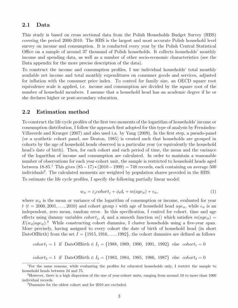
2.1 Data
This study is based on cross sectional data from the Polish Households Budget Survey (HBS)covering the period 2000-2010. The HBS is the largest and most accurate Polish household levelsurvey on income and consumption. It is conducted every year by the Polish Central StatisticalOffice on a sample of around 37 thousand of Polish households. It collects households’ monthlyincome and spending data, as well as a number of other socio-economic characteristics (see theData appendix for the more precise description of the data).
To construct the income and consumption profiles, I use individual households’ total monthlyavailable net income and total monthly expenditures on consumer goods and services, adjustedfor inflation with the consumer price index. To control for family size, an OECD square rootequivalence scale is applied, i.e. income and consumption are divided by the square root of thenumber of household members. I assume that a household head has an academic degree if he orshe declares higher or post-secondary education.
2.2 Estimation method
To construct the life cycle profiles of the first two moments of the logarithm of households’ income orconsumption distribution, I follow the approach first adopted for this type of analysis by Fernandez-Villaverde and Krueger (2007) and also used i.a. by Yang (2009). In the first step, a pseudo-panel(or a synthetic cohort panel, see Deaton, 1985) is created such that households are grouped incohorts by the age of household heads observed in a particular year (or equivalently the householdhead’s date of birth). Then, for each cohort and each period of time, the mean and the varianceof the logarithm of income and consumption are calculated. In order to maintain a reasonablenumber of observations for each year-cohort unit, the sample is restricted to household heads agedbetween 18-85.1 This gives (85−17)∗ (2010−1999) = 748 records, each containing on average 500individuals2. The calculated moments are weighted by population shares provided in the HBS.
To estimate the life cycle profiles, I specify the following partially linear model:
wit = pjcohortj + φtdt +m(ageit) + εit, (1)
where wit is the mean or variance of the logarithm of consumption or income, evaluated for yeart (t = 2000, 2001, . . . , 2010) and cohort group i with age of household head ageit, while εit is anindependent, zero mean, random error. In this specification, I control for cohort, time and ageeffects using dummy variables cohortj, dt and a smooth function m() which satisfies m(ageit) =E(wit|ageit).3 While constructing cohort dummies, I cluster households using a five-year span.More precisely, having assigned to every cohort the date of birth of household head (in shortDateOfBirth) from the set I = {1915, 1916, . . . , 1992}, the cohort dummies are defined as follows
cohort1 = 1 if DateOfBirth ∈ I1 = {1988, 1989, 1990, 1991, 1992} else cohort1 = 0
cohort2 = 1 if DateOfBirth ∈ I2 = {1983, 1984, 1985, 1986, 1987} else cohort2 = 0
1For the same reasons, while evaluating the profiles for educated households only, I restrict the sample tohousehold heads between 24 and 75.
2However, there is a high dispersion of the size of year-cohort units, ranging from around 10 to more than 1000individual records.
3Dummies for the oldest cohort and for 2010 are excluded.
3

...
cohortj = 1 if DateOfBirth ∈ Ij ={1988−5(j−1), 1989−5(j−1), 1990−5(j−1), 1991−5(j−1), 1992−5(j−1)} else cohortj = 0.
Further, assuming that index i also indicates the date of birth of household head, it holds thati ∈ Ij. Reducing the number of estimated dummy-cohort parameters with five-year spans eliminatesthe identification problem4 and increases the number of degrees of freedom.
According to equation (1), the dependent variable is explained by two components. The first one isparametric (linear) and consists of the cohort and year dummies. The other part is a nonparametricrelationship linking the dependent variable to household heads’ age. The model is estimated usinga two-step Speckman (1988) procedure, which is a combination of the ordinary least squares and astandard kernel smoothing estimator.5 A detailed description of this procedure and its applicationto a life cycle framework is provided i.a. in the technical appendix to Fernandez-Villaverde andKrueger (2007).The bandwidth parameter h is set to 2 and was chosen using a cross-validationmethod carried out on the average logarithm of consumption (the detailed results are availableupon request).
Finally, to quantify the significance of the age-profiles’ estimates, the 95% bootstrap confidenceintervals (based on 500 replications) are calculated.. As discussed in the literature (see Hall, 1992;Neumann, 1995), in nonparametric regression the bootstrap method has an estimation bias. Oneway of dealing with this problem is to impose undersmoothing. Hence, while bootstrapping I setthe bandwidth parameter (h) to 1.8.
2.3 Average life cycle profile of income and consumption
Figure 1 presents the average logarithm of households’ available income6 with and without ad-justment for the number of households members, while Table 1 summaries the changes in averagereceived income. The average income profile exhibits a hump-shaped pattern known from the liter-ature. Most notably, and consistently with Alessie et al. (1997), while a sharp increase is observedbelow the age of 30, average income growth becomes moderate when household head is between30 and 50. This pattern is even more evident when one controls for the household size.
One possible explanation for the rapid increase in the average income observed for householdsbetween 18 and 25 is a significant number of individuals who postpone their professional careerin order to increase qualifications (or education). According to the 2009 HBS, 25% of younghousehold heads (aged from 18 to 25) declared that they were not looking for a job because theywere still learning. However, excluding these households from the sample does not change theobserved pattern significantly.
4Otherwise, the linear dependence of variables requires dropping one additional dummy and hence imposingadditional assumptions. The common way of dealing with this problem is to attribute trend to cohort effectsand apply a normalization which guarantees that time effects sum up to zero (see Deaton, 1997). However, thisprocedure fails if the number of years in the sample is small and/or if separating a trend from transitory shocksis difficult. In particular, distinguishing between trend and cycle is hard if one relies on data from a transitioneconomy.
5The nonparametric component is estimated using a Nadaraya–Watson estimator with an Epanechnikov kernel.6More precisely, Figure 1 depicts the estimates for households born between 1958 and 1962, calculated for 2007
(i.e. π7 + φ2007 + m(age)). This applies to all life cycle profiles presented in the article.
4
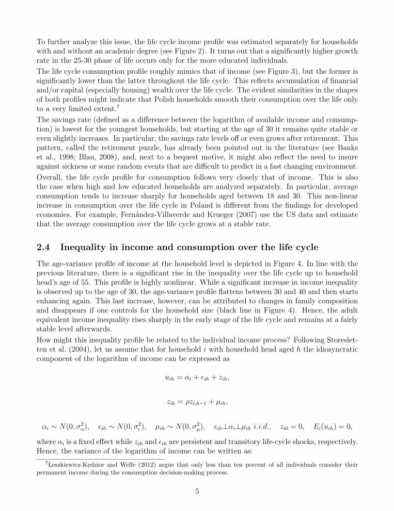
To further analyze this issue, the life cycle income profile was estimated separately for householdswith and without an academic degree (see Figure 2). It turns out that a significantly higher growthrate in the 25-30 phase of life occurs only for the more educated individuals.
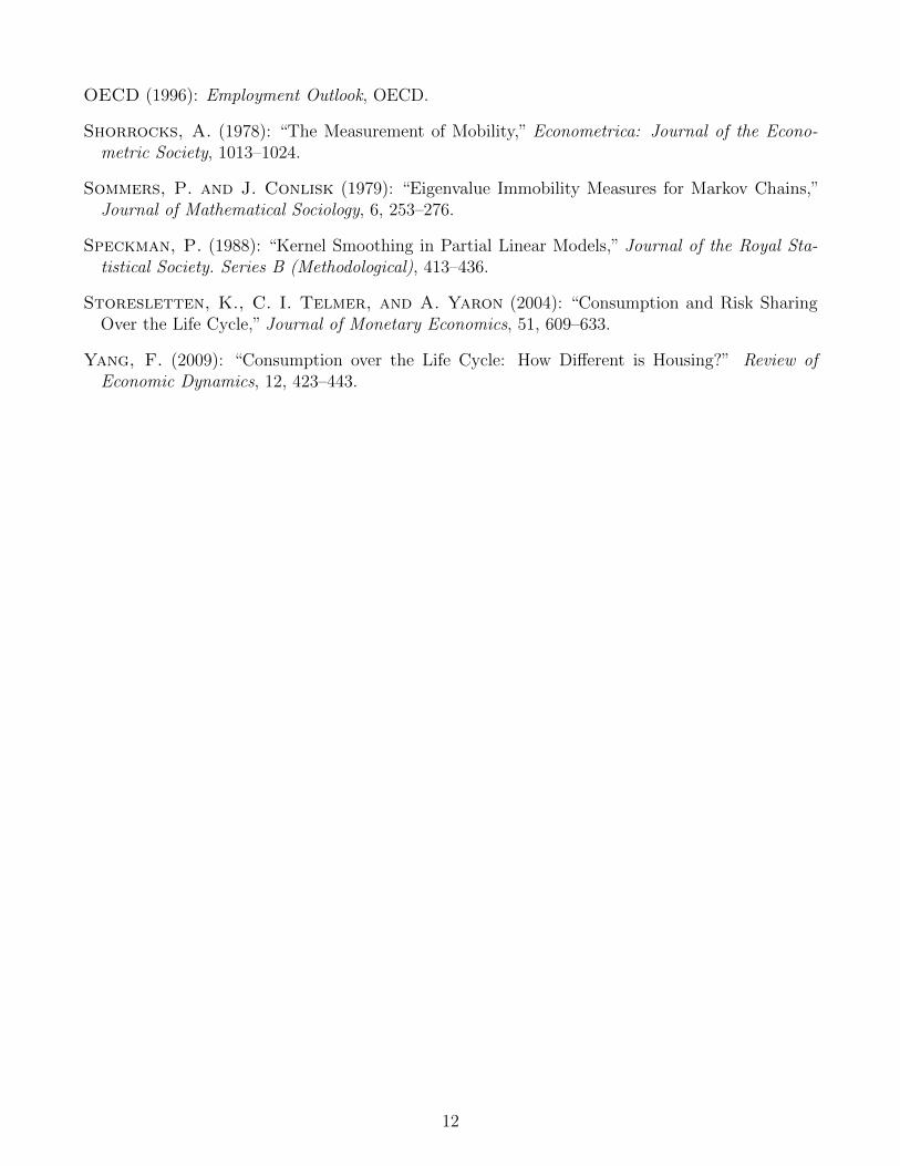
The life cycle consumption profile roughly mimics that of income (see Figure 3), but the former issignificantly lower than the latter throughout the life cycle. This reflects accumulation of financialand/or capital (especially housing) wealth over the life cycle. The evident similarities in the shapesof both profiles might indicate that Polish households smooth their consumption over the life onlyto a very limited extent.7
The savings rate (defined as a difference between the logarithm of available income and consump-tion) is lowest for the youngest households, but starting at the age of 30 it remains quite stable oreven slightly increases. In particular, the savings rate levels off or even grows after retirement. Thispattern, called the retirement puzzle, has already been pointed out in the literature (see Bankset al., 1998; Blau, 2008), and, next to a bequest motive, it might also reflect the need to insureagainst sickness or some random events that are difficult to predict in a fast changing environment.
Overall, the life cycle profile for consumption follows very closely that of income. This is alsothe case when high and low educated households are analyzed separately. In particular, averageconsumption tends to increase sharply for households aged between 18 and 30. This non-linearincrease in consumption over the life cycle in Poland is different from the findings for developedeconomies. For example, Fernandez-Villaverde and Krueger (2007) use the US data and estimatethat the average consumption over the life cycle grows at a stable rate.
2.4 Inequality in income and consumption over the life cycle
The age-variance profile of income at the household level is depicted in Figure 4. In line with theprevious literature, there is a significant rise in the inequality over the life cycle up to householdhead’s age of 55. This profile is highly nonlinear. While a significant increase in income inequalityis observed up to the age of 30, the age-variance profile flattens between 30 and 40 and then startsenhancing again. This last increase, however, can be attributed to changes in family compositionand disappears if one controls for the household size (black line in Figure 4). Hence, the adultequivalent income inequality rises sharply in the early stage of the life cycle and remains at a fairlystable level afterwards.
How might this inequality profile be related to the individual income process? Following Storeslet-ten et al. (2004), let us assume that for household i with household head aged h the idiosyncraticcomponent of the logarithm of income can be expressed as
uih = αi + εih + zih,
zih = ρzi,h−1 + µih,
αi ∼ N(0, σ2α), εih ∼ N(0, σ2
ε ), µih ∼ N(0, σ2µ), εih⊥αi⊥µih i.i.d., zi0 = 0, Ei(uih) = 0,
where αi is a fixed effect while zih and εih are persistent and transitory life-cycle shocks, respectively.Hence, the variance of the logarithm of income can be written as:
7Leszkiewicz-K ↪edzior and Welfe (2012) argue that only less than ten percent of all individuals consider theirpermanent income during the consumption decision-making process.
5
V ari(uih) = sv2a
+ sv2ε + sv
2m
∑h−1
j=0ρ2j.
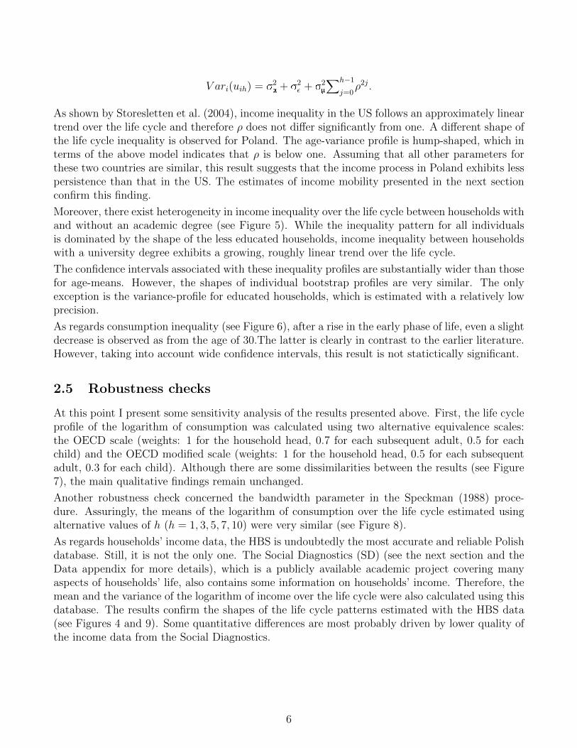
As shown by Storesletten et al. (2004), income inequality in the US follows an approximately lineartrend over the life cycle and therefore ρ does not differ significantly from one. A different shape ofthe life cycle inequality is observed for Poland. The age-variance profile is hump-shaped, which interms of the above model indicates that ρ is below one. Assuming that all other parameters forthese two countries are similar, this result suggests that the income process in Poland exhibits lesspersistence than that in the US. The estimates of income mobility presented in the next sectionconfirm this finding.
Moreover, there exist heterogeneity in income inequality over the life cycle between households withand without an academic degree (see Figure 5). While the inequality pattern for all individualsis dominated by the shape of the less educated households, income inequality between householdswith a university degree exhibits a growing, roughly linear trend over the life cycle.
The confidence intervals associated with these inequality profiles are substantially wider than thosefor age-means. However, the shapes of individual bootstrap profiles are very similar. The onlyexception is the variance-profile for educated households, which is estimated with a relatively lowprecision.
As regards consumption inequality (see Figure 6), after a rise in the early phase of life, even a slightdecrease is observed as from the age of 30.The latter is clearly in contrast to the earlier literature.However, taking into account wide confidence intervals, this result is not statictically significant.
2.5 Robustness checks
At this point I present some sensitivity analysis of the results presented above. First, the life cycleprofile of the logarithm of consumption was calculated using two alternative equivalence scales:the OECD scale (weights: 1 for the household head, 0.7 for each subsequent adult, 0.5 for eachchild) and the OECD modified scale (weights: 1 for the household head, 0.5 for each subsequentadult, 0.3 for each child). Although there are some dissimilarities between the results (see Figure7), the main qualitative findings remain unchanged.
Another robustness check concerned the bandwidth parameter in the Speckman (1988) proce-dure. Assuringly, the means of the logarithm of consumption over the life cycle estimated usingalternative values of h (h = 1, 3, 5, 7, 10) were very similar (see Figure 8).
As regards households’ income data, the HBS is undoubtedly the most accurate and reliable Polishdatabase. Still, it is not the only one. The Social Diagnostics (SD) (see the next section and theData appendix for more details), which is a publicly available academic project covering manyaspects of households’ life, also contains some information on households’ income. Therefore, themean and the variance of the logarithm of income over the life cycle were also calculated using thisdatabase. The results confirm the shapes of the life cycle patterns estimated with the HBS data(see Figures 4 and 9). Some quantitative differences are most probably driven by lower quality ofthe income data from the Social Diagnostics.
6
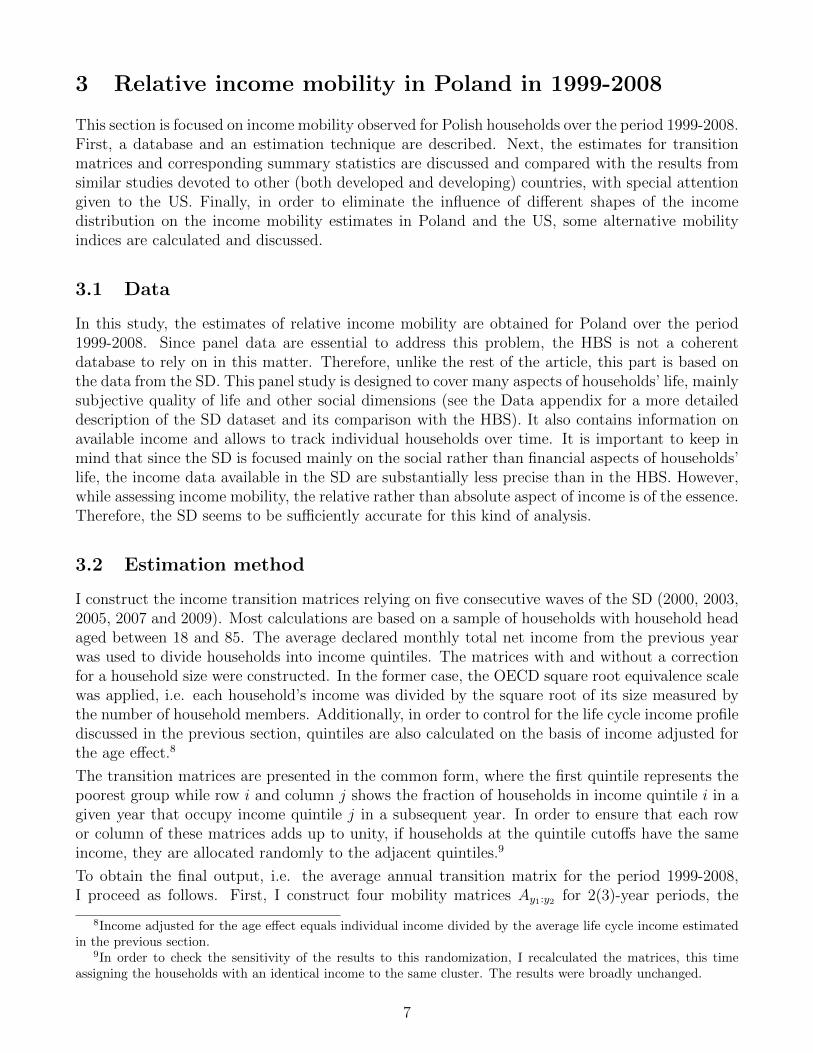
3 Relative income mobility in Poland in 1999-2008
This section is focused on income mobility observed for Polish households over the period 1999-2008.First, a database and an estimation technique are described. Next, the estimates for transitionmatrices and corresponding summary statistics are discussed and compared with the results fromsimilar studies devoted to other (both developed and developing) countries, with special attentiongiven to the US. Finally, in order to eliminate the influence of different shapes of the incomedistribution on the income mobility estimates in Poland and the US, some alternative mobilityindices are calculated and discussed.
3.1 Data
In this study, the estimates of relative income mobility are obtained for Poland over the period1999-2008. Since panel data are essential to address this problem, the HBS is not a coherentdatabase to rely on in this matter. Therefore, unlike the rest of the article, this part is based onthe data from the SD. This panel study is designed to cover many aspects of households’ life, mainlysubjective quality of life and other social dimensions (see the Data appendix for a more detaileddescription of the SD dataset and its comparison with the HBS). It also contains information onavailable income and allows to track individual households over time. It is important to keep inmind that since the SD is focused mainly on the social rather than financial aspects of households’life, the income data available in the SD are substantially less precise than in the HBS. However,while assessing income mobility, the relative rather than absolute aspect of income is of the essence.Therefore, the SD seems to be sufficiently accurate for this kind of analysis.
3.2 Estimation method
I construct the income transition matrices relying on five consecutive waves of the SD (2000, 2003,2005, 2007 and 2009). Most calculations are based on a sample of households with household headaged between 18 and 85. The average declared monthly total net income from the previous yearwas used to divide households into income quintiles. The matrices with and without a correctionfor a household size were constructed. In the former case, the OECD square root equivalence scalewas applied, i.e. each household’s income was divided by the square root of its size measured bythe number of household members. Additionally, in order to control for the life cycle income profilediscussed in the previous section, quintiles are also calculated on the basis of income adjusted forthe age effect.8
The transition matrices are presented in the common form, where the first quintile represents thepoorest group while row i and column j shows the fraction of households in income quintile i in agiven year that occupy income quintile j in a subsequent year. In order to ensure that each rowor column of these matrices adds up to unity, if households at the quintile cutoffs have the sameincome, they are allocated randomly to the adjacent quintiles.9
To obtain the final output, i.e. the average annual transition matrix for the period 1999-2008,I proceed as follows. First, I construct four mobility matrices Ay1:y2 for 2(3)-year periods, the
8Income adjusted for the age effect equals individual income divided by the average life cycle income estimatedin the previous section.
9In order to check the sensitivity of the results to this randomization, I recalculated the matrices, this timeassigning the households with an identical income to the same cluster. The results were broadly unchanged.
7
multiplication of which gives me the nine-year transition matrix (A2000:2009 = A2000:2003 ∗A2003:2005 ∗A2005:2007 ∗ A2007:2009).10 The final one-year period matrix (B) satisfies the following equation:
B = A1/92000:2009 = V D1/9V −1, where V DV −1 (D - diagonal) is a spectral decomposition of matrix
A2000:2009.11
Calculating the average transition matrix is appealing for at least two reasons. First, it allows touse all available information and maintain the statistical correctness of the results. Second, sucha transformation is very convenient for comparative purposes.
On the basis of the obtained matrices, the following summary indicators of income mobility arecalculated: (1) the average quintile move (see Khor and Pencavel, 2006 for the formula), (2) theimmobility ratio, defined as the fraction of households that remain in the same quintile (3) theadjusted immobility ratio, defined as the fraction of those who remain in the same quintile or moveto an adjacent quintile, (4) the distance between the calculated matrix and the perfect mobilitybenchmark proposed by Shorrocks (1978), i.e. one minus the second greatest eigenvalue of a matrix,and (5) the Sommers and Conlisk (1979) measure of mobility, calculated as one minus the productof all eigenvalues.
3.3 Results
The transition matrices and corresponding income mobility indices are presented in Tables 2 and3. The chi-square test for the symmetry of the matrices (see Khor and Pencavel, 2010 for an exactformula) cannot be rejected at any conventional level of confidence. At least fifteen percent ofhouseholds with household head aged between 18 and 85 who occupy the lowest quintile in oneperiod leave that quintile next year (see the left matrix from the top panel of Table 2). On the otherhand, less than eighty percent of Polish households remain in the top rank in two subsequent years.Hence, staying in the same quintile appears to be more persistent for the poorest households. Thisproperty, also observed in Russia (see Lukiyanova and Oshchepkov, 2011), is not characteristicfor the US (see Table 4). Moreover, in the center of the income distribution there is even moremobility with probabilities of remaining in the same rank for the second, third and fourth quintileslying between 60-70 percent.
Since the main goal of this study is to analyze idiosyncratic aspects of income mobility, thoseindividuals’ movements in income distribution that are caused by choosing between educationand work or resulting from retirement are not of a particular interest. However, restricting thesample to working-age households (a household head aged between 25 and 65) turns out to add toincome mobility, decreasing the immobility ratio from 0.72 to 0.68. This result is a consequence ofexcluding from the sample retired households whose income shows less variability. Nevertheless,the difference in income mobility between working-age households and the total sample is rathersmall. Further, adjusting for the households size increases slightly individuals’ movements inincome distribution, while imposing correction for the life cycle income profile leaves the estimatesof income mobility broadly unchanged. Examining urban and rural households separately does
10These matrices are calculated based on the following pairs of the SD waves: 2000 and 2003, 2003 and 2005,2005 and 2007, 2007 and 2009. For each of these pairs there is roughly 2000-3300 individual records. Obtaining thenine-year transition matrix A2000:2009 directly is inefficient as it would rely on less than 1000 records.
11Distinct eigenvalues are a sufficient condition for the existence of such a decomposition of a quadratic matrix.However, this method of calculating the m-period average annual transition matrix has its limitations. First, with“m” being an even number, there might be more than one solution. Second, the average transition matrix mightnot exist, i.e. B can have negative entries if transition probabilities substantially vary over time.
8
not show significant differences between these two groups, either. Generally, the results obtainedfor Poland are fairly robust to alternative specifications.
How income-mobile are Polish households in comparison to other countries? First, I focus on thedifference vis-a-vis the developed economies. Since the existing cross-country analyses (Aabergeet al., 2002; Burkhauser et al., 1998) clearly show that the differences in income mobility betweenthe US and old EU countries are usually found to be very small, and also income mobility in the USwas a topic of a number of comprehensive empirical studies, I use this country as a benchmark. Theestimates of income mobility in the US are taken from Dıaz-Gimenez et al. (2011) and annualizedusing the eigenvalue decomposition described in the previous subsection.12 Table 3 shows thesummary results while the average annual transition matrix for the US is presented in Table 4.
Polish households appear to be more mobile in terms of income than the American ones accordingto all mobility indices.13 The smallest difference is observed for the adjusted immobility ratio,which suggests that the main difference between Polish and US households’ mobility concernsmovements between adjacent quintiles.
As regards the mobility indices for other countries, direct comparisons are difficult due to method-ological differences (sample, equivalence scales, income measures etc.) and hence one needs to becautious while interpreting the results. A summary of immobility measures for selected countrieswith a short description of the main assumptions imposed are presented in Table 5. The reportedresults might suggest that the degree of mobility in Poland is more similar to that observed inChina and Russia, i.e. developing or transition economies, than to that obtained for developedcountries.
3.3.1 Dispersion of income distribution and income mobility
One of the factors that can be responsible for the dissimilarities in income mobility between differentcountries is inequality in income distribution. Generally, the narrower the income distribution, themore probable the jump for an individual from one quintile to another.
The quintiles of income in Poland and the US are reported in Table 6. According to these statistics,the income distribution in the US seems to be more disperse than in Poland. In particular, in theUS (based on data from 2007, taken from Dıaz-Gimenez et al., 2011), the third quintile of incomedistribution was roughly 2.9 times greater than the first one, while an analogous statistics forPoland (according to the Polish HBS from 2010) was only 2.1414.
I next try to assess, to what extent the dissimilarities in income mobility between Polish andAmerican households are driven by the differences in the shapes of their income distributions. Tothis end, an artificial distribution of income for Polish households is generated, such that it mimicsthat observed in the US. More specifically, the first quintile is kept unchanged and the relationbetween the first and the rest of quintiles is taken from the US data, see Table 6. Then, the averageprobability of remaining in the same “simulated quintile” for two consecutive years is quantifiedand shown in Table 7, together with the estimates calculated on the basis of the observed quintilesfor Poland and the US. Except for the lowest and highest quintiles, these artificially generated
12The results are very similar if one uses instead individual income tax returns as the data source (see Table 4for annual transition matrices calculated on the basis of these two studies).
13To ensure comparability to the US, I use here the results for Poland obtained for the whole sample withoutadjusting for family size and age effect (bolded row in Table 3).
14Based on the Polish HBS from 2000-2010, the relation between income quintiles in Poland was quite stable overtime. The same pattern is observed while comparing the means and medians between the quintiles.
9
probabilities are higher than those reported for the original data. In addition, there is a slightimprovement in income immobility ratio, but still its value is significantly lower than that in theUnited States. Hence, adjusting for the inequality in income distribution reduces only slightly theobserved differences in income mobility between Poland and the US.
4 Concluding remarks
In this paper I investigated the life cycle income and consumption patterns in Poland, relying onthe estimates of the income and consumption distributions as well as the transition matrices ofrelative income mobility.
The main findings are as follows. The average income over the life cycle follows an inverted U-shape. For the educated households, the most intense increase is observed in the early phase oflife, up to the age of 30. The average consumption over the life cycle mimics quite closely theaverage income.
In contrast to a roughly linear increasing trend of income inequality over the life cycle obtainedfor the US, the age-variance profile for Poland is humped-shaped. More precisely, the incomeinequality increases sharply at the early phase of life and then remains quite stable up to theretirement age. This finding might indicate less persistence in individual income process. Indeed,the estimates of transition matrices for Poland confirm that relative income mobility is higher thanthat observed in developed countries.
Interestingly, the age-variance profile for more educated households differs from that obtained forthe whole population and is similar to that for all US households. Hence, the rapid increase in theshare of individuals with an academic degree that was observed in Poland during the economictransition should result in a gradual convergence of income inequality profile to that obtained fordeveloped economies.
A natural extension of this study would be to investigate how the patterns obtained for Polandcan be generalized to other economies in transition, especially ex-communist Central and EasternEuropean countries. It would also be interesting to examine to what extent the differences betweenPoland and developed economies that I identified at the micro level translate into different proper-ties of macroeconomic aggregates. In this respect, general equilibrium models with heterogeneoushouseholds could serve as a useful laboratory. I leave these questions for future research.
References
Aaberge, R., A. Bjorklund, M. Jantti, M. Palme, P. Pedersen, N. Smith, andT. Wennemo (2002): “Income Inequality and Income Mobility in the Scandinavian CountriesCompared to the United States,” Review of Income and Wealth, 48, 443–469.
Abe, N. and T. Yamada (2009): “Nonlinear Income Variance Profiles and Consumption Inequal-ity over the Life Cycle,” Journal of the Japanese and International Economies, 23, 344–366.
Alessie, R., A. Lusardi, and T. Aldershof (1997): “Income and Wealth over the Life Cycle:Evidence from Panel Data,” Review of Income and Wealth, 43, 1–32.
Auten, G. E. and G. Gee (2007): “Income Mobility in the U.S. from 1996 to 2005,” Report,Department of Treasury.
10
Banks, J., R. Blundell, and S. Tanner (1998): “Is There a Retirement-Savings Puzzle?”American Economic Review, 88, 769–788.
Blau, D. (2008): “Retirement and Consumption in a Life Cycle Model,” Journal of Labor Eco-nomics, 26, 35–71.
Burkhauser, R., D. Holtz-Eakin, and S. Rhody (1998): “Mobility and Inequality in the1980s: A Cross-National Comparison of the United States and Germany,” in The Distributionof Welfare and Household Production, ed. by K. Jenkins and V. Praag, Elsevier, 111–175.
Cagetti, M. (2003): “Wealth Accumulation over the Life Cycle and Precautionary Savings,”Journal of Business and Economic Statistics, 21, 339–353.
Dıaz-Gimenez, J., A. Glover, and J.-V. Rıos-Rull (2011): “Facts on the Distributions ofEarnings, Income, and Wealth in the United States: 2007 Update,”Quarterly Review, 34, 2–31.
Deaton, A. (1985): “Panel Data from Time Series of Cross-Sections,” Journal of Econometrics,30, 109–126.
——— (1997): The Analysis of Household Surveys: A Microeconomic Approach to DevelopmentPolicy, Johns Hopkins University Press.
Deaton, A. and C. Paxson (1994): “Intertemporal Choice and Inequality,” Journal of PoliticalEconomy, 102, 437–67.
Fabig, H. (1998): “Income Mobility in International Comparison - An Empirical Analysis withPanel Data,” Report, Goethe University Frankfurt.
Fernandez-Villaverde, J. and D. Krueger (2007): “Consumption over the Life Cycle:Facts from Consumer Expenditure Survey Data,” The Review of Economics and Statistics, 89,552–565.
Gourinchas, P. and J. Parker (2002): “Consumption Over the Life Cycle,” Econometrica,70, 47–89.
Hall, P. (1992): “Effect of Bias Estimation on Coverage Accuracy of Bootstrap ConfidenceIntervals for a Probability Density,” The Annals of Statistics, 675–694.
Khor, N. and J. Pencavel (2006): “Income Mobility of Individuals in China and the UnitedStates,” Economics of Transition, 14, 417–458.
——— (2010): “Evolution of Income Mobility in the People’s Republic of China: 1991-2002,”ADBEconomics Working Paper Series.
Leszkiewicz-K ↪edzior, K. and W. Welfe (2012): “Consumption Function for Poland. Is LifeCycle Hypothesis Legitimate?” Bank i Kredyt, 43, 5–20.
Lukiyanova, A. and A. Oshchepkov (2011): “Income mobility in Russia (2000–2005),” Eco-nomic Systems, 36, 46–64.
Neumann, M. (1995): “Automatic Bandwidth Choice and Confidence Intervals in NonparametricRegression,” The Annals of Statistics, 23, 1937–1959.
11
OECD (1996): Employment Outlook, OECD.
Shorrocks, A. (1978): “The Measurement of Mobility,” Econometrica: Journal of the Econo-metric Society, 1013–1024.
Sommers, P. and J. Conlisk (1979): “Eigenvalue Immobility Measures for Markov Chains,”Journal of Mathematical Sociology, 6, 253–276.
Speckman, P. (1988): “Kernel Smoothing in Partial Linear Models,” Journal of the Royal Sta-tistical Society. Series B (Methodological), 413–436.
Storesletten, K., C. I. Telmer, and A. Yaron (2004): “Consumption and Risk SharingOver the Life Cycle,” Journal of Monetary Economics, 51, 609–633.
Yang, F. (2009): “Consumption over the Life Cycle: How Different is Housing?” Review ofEconomic Dynamics, 12, 423–443.
12

5 Figures and tables
Figure 1: Average income over the life cycle
20 30 40 50 60 70 80
6.6
6.8
7.0
7.2
7.4
7.6
7.8
age of household head
mea
n of
the
loga
rithm
of i
ncom
e
Notes: black line - square root equivalence scale; blue line - household level; dashed lines - 95%bootstrap confidence intervals; estimates based on the Polish HBS 2000-2010.
Figure 2: Average income over the life cycle by educational groups
20 30 40 50 60 70
6.6
6.8
7.0
7.2
7.4
7.6
7.8
age of household head
mea
n of
the
loga
rithm
of i
ncom
e
Notes: black line - without an academic degree; blue line - with an academic degree; dashedlines - 95% bootstrap confidence intervals; estimates based on the Polish HBS 2000-2010, adultequivalent (square root equivalence scale).
13
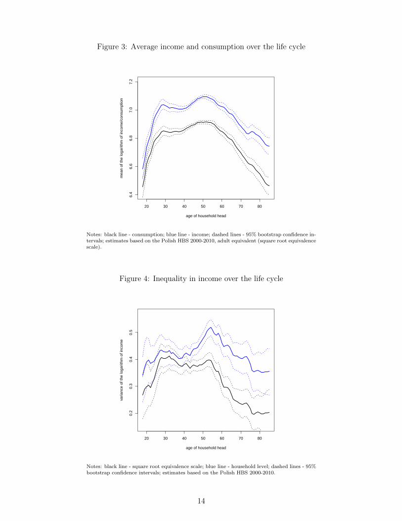
Figure 3: Average income and consumption over the life cycle
20 30 40 50 60 70 80
6.4
6.6
6.8
7.0
7.2
age of household head
mea
n of
the
loga
rithm
of i
ncom
e/co
nsum
ptio
n
Notes: black line - consumption; blue line - income; dashed lines - 95% bootstrap confidence in-tervals; estimates based on the Polish HBS 2000-2010, adult equivalent (square root equivalencescale).
Figure 4: Inequality in income over the life cycle
20 30 40 50 60 70 80
0.2
0.3
0.4
0.5
age of household head
varia
nce
of th
e lo
garit
hm o
f inc
ome
Notes: black line - square root equivalence scale; blue line - household level; dashed lines - 95%bootstrap confidence intervals; estimates based on the Polish HBS 2000-2010.
14
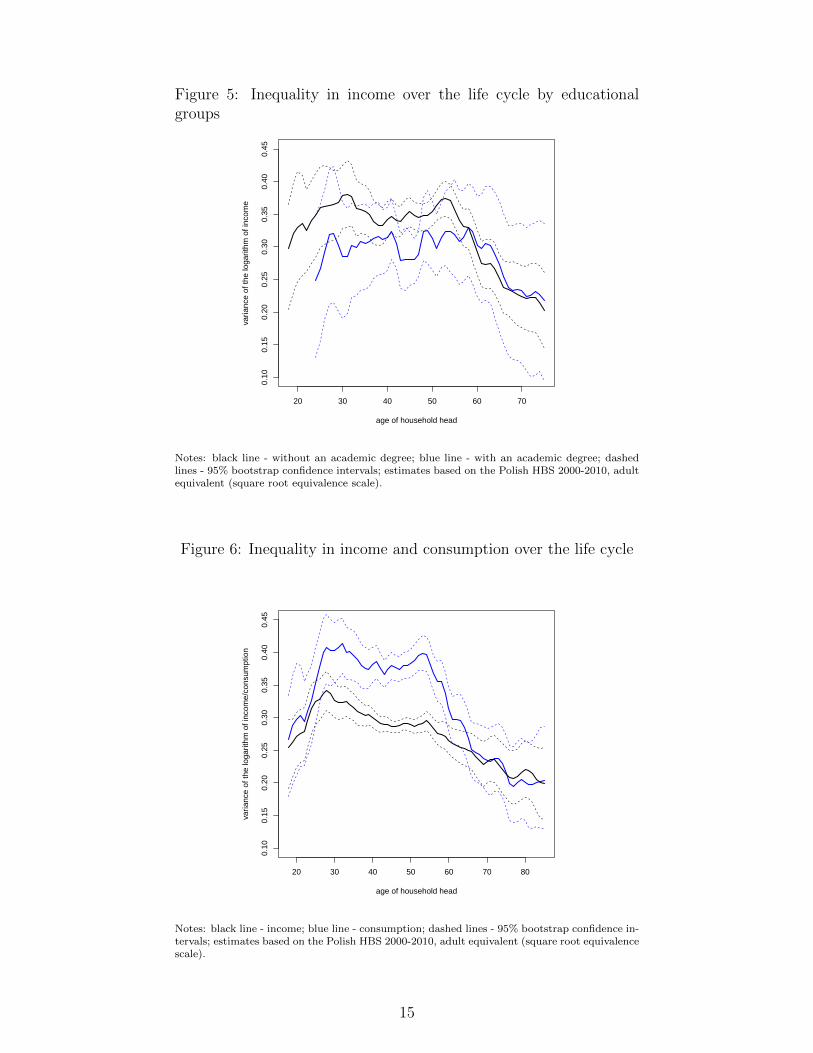
Figure 5: Inequality in income over the life cycle by educationalgroups
20 30 40 50 60 70
0.10
0.15
0.20
0.25
0.30
0.35
0.40
0.45
age of household head
varia
nce
of th
e lo
garit
hm o
f inc
ome
Notes: black line - without an academic degree; blue line - with an academic degree; dashedlines - 95% bootstrap confidence intervals; estimates based on the Polish HBS 2000-2010, adultequivalent (square root equivalence scale).
Figure 6: Inequality in income and consumption over the life cycle
20 30 40 50 60 70 80
0.10
0.15
0.20
0.25
0.30
0.35
0.40
0.45
age of household head
varia
nce
of th
e lo
garit
hm o
f inc
ome/
cons
umpt
ion
Notes: black line - income; blue line - consumption; dashed lines - 95% bootstrap confidence in-tervals; estimates based on the Polish HBS 2000-2010, adult equivalent (square root equivalencescale).
15
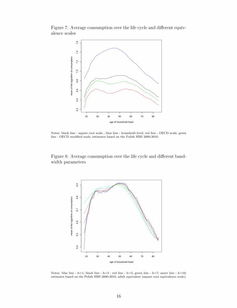
Figure 7: Average consumption over the life cycle and different equiv-alence scales
20 30 40 50 60 70 80
6.2
6.4
6.6
6.8
7.0
7.2
7.4
7.6
age of household head
mea
n of
the
loga
rithm
of c
onsu
mpt
ion
Notes: black line - square root scale ; blue line - household level; red line - OECD scale; greenline - OECD modified scale; estimates based on the Polish HBS 2000-2010.
Figure 8: Average consumption over the life cycle and different band-width parameters
20 30 40 50 60 70 80
6.4
6.5
6.6
6.7
6.8
6.9
age of household head
mea
n of
the
loga
rithm
of c
onsu
mpt
ion
Notes: blue line - h=1; black line - h=3 ; red line - h=5; green line - h=7; azure line - h=10;estimates based on the Polish HBS 2000-2010, adult equivalent (square root equivalence scale).
16
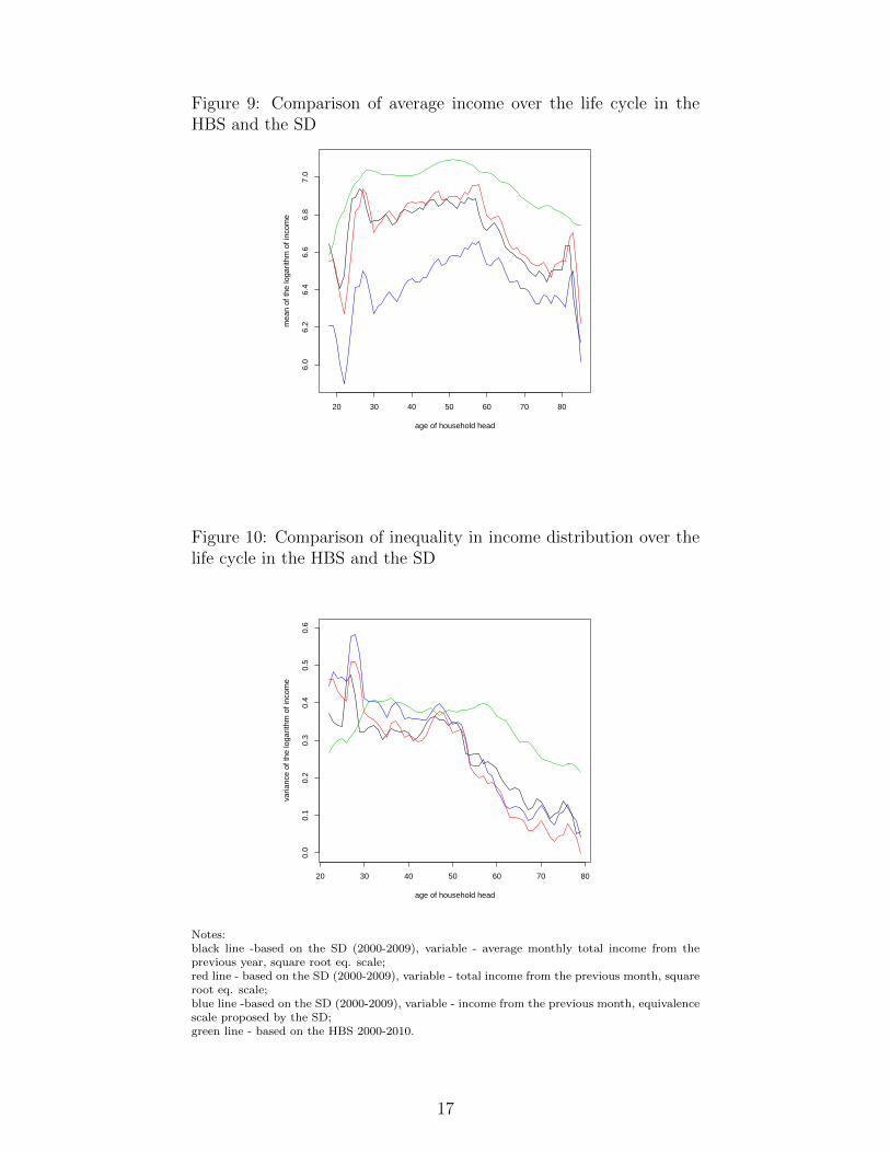
Figure 9: Comparison of average income over the life cycle in theHBS and the SD
20 30 40 50 60 70 80
6.0
6.2
6.4
6.6
6.8
7.0
age of household head
mea
n of
the
loga
rithm
of i
ncom
e
Figure 10: Comparison of inequality in income distribution over thelife cycle in the HBS and the SD
20 30 40 50 60 70 80
0.0
0.1
0.2
0.3
0.4
0.5
0.6
age of household head
varia
nce
of th
e lo
garit
hm o
f inc
ome
Notes:black line -based on the SD (2000-2009), variable - average monthly total income from theprevious year, square root eq. scale;red line - based on the SD (2000-2009), variable - total income from the previous month, squareroot eq. scale;blue line -based on the SD (2000-2009), variable - income from the previous month, equivalencescale proposed by the SD;green line - based on the HBS 2000-2010.
17

Table 1: Changes in household’s average available income over the life cycleHousehold head aged between Household level Adult equivalent
25-20 31.6% 23.0%
30-25 14.0% 6.2%
35-30 5.8% -1.7%
40-35 3.2% -0.4%
45-40 3.7% 4.8%
50-45 -1.9% 3.6%
55-50 -8.9% -1.8%
60-55 -11.3% -4.9%
65-60 -9.5% -5.5%
70-65 -12.4% -8.8%
75-70 -6.4% -3.9%
80-75 -4.6% -3.3%
85-80 -7.1% -6.5%
Table 2: Average annual income transition matrices, Polish households 1999-2008
Sample: household head aged between 18 and 85 Sample: household head aged between 18 and 85
Eq. scale: NO, adjusted for age effect: NO Eq. scale: YES, adjusted for age effect: NO
Income Quintiles Income Quintiles
Lowest Second Middle Fourth Highest Lowest Second Middle Fourth Highest
Lowest 0.84 0.11 0.03 0.02 0.01 Lowest 0.79 0.13 0.05 0.02 0.01
Second 0.11 0.70 0.12 0.05 0.02 Second 0.14 0.63 0.15 0.06 0.03
Middle 0.03 0.15 0.64 0.15 0.03 Middle 0.05 0.17 0.58 0.16 0.03
Fourth 0.01 0.03 0.16 0.63 0.16 Fourth 0.01 0.05 0.18 0.62 0.14
Highest 0.01 0.01 0.05 0.16 0.78 Highest 0.01 0.02 0.04 0.14 0.79
Sample: household head aged between 25 and 65 Sample: household head aged between 18 and 85
Eq. scale: NO, adjusted for age effect: NO Eq. scale: YES, adjusted for age effect: YES
Income Quintiles Income Quintiles
Lowest Second Middle Fourth Highest Lowest Second Middle Fourth Highest
Lowest 0.82 0.11 0.04 0.02 0.01 Lowest 0.80 0.13 0.04 0.02 0.01
Second 0.12 0.67 0.14 0.06 0.01 Second 0.12 0.63 0.17 0.05 0.02
Middle 0.04 0.15 0.59 0.18 0.04 Middle 0.05 0.18 0.58 0.16 0.04
Fourth 0.01 0.06 0.19 0.56 0.19 Fourth 0.02 0.04 0.18 0.62 0.14
Highest 0.01 0.01 0.03 0.19 0.76 Highest 0.01 0.02 0.04 0.14 0.79
18

Table 3: Summary of income mobility, one-year horizon, indices for Poland and the US
imm
obilit
yra
tio
adju
sted
imm
ob
ilit
yra
tio
aver
age
qu
inti
lem
ove
1−λ2
(Sh
orr
ock
s,1978)
1−λ1∗...∗λn
(Som
mer
sand
Con
lisk
,1979)
eq. scale age adj. sample urban/rural
POLAND NO NO age 18-85 both 0.72 0.94 0.36 0.14 0.85
NO NO age 25-65 both 0.68 0.93 0.41 0.16 0.90
YES NO age 18-85 both 0.68 0.92 0.42 0.17 0.89
YES YES age 18-85 both 0.68 0.93 0.41 0.16 0.89
NO NO age 18-85 urban 0.72 0.94 0.36 0.13 0.85
NO NO age 18-85 rural 0.70 0.93 0.40 0.15 0.85
the US NO NO both 0.87 0.98 0.15 0.05 0.53
perfect mobility 0.20 0.52 1.60 1.00 1.00
complete immobility (identity matrix) 1.00 1.00 0.00 0.00 0.00
19
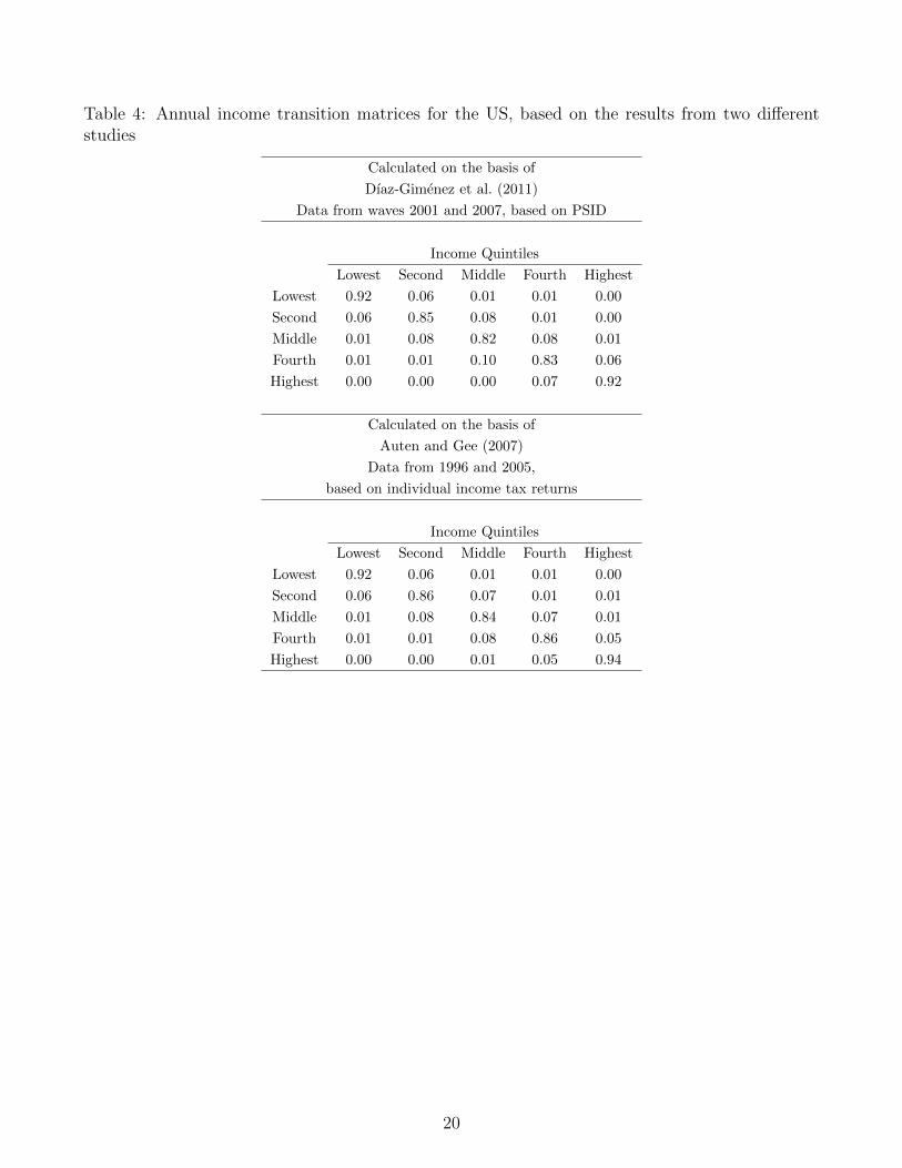
Table 4: Annual income transition matrices for the US, based on the results from two differentstudies
Calculated on the basis of
Dıaz-Gimenez et al. (2011)
Data from waves 2001 and 2007, based on PSID
Income Quintiles
Lowest Second Middle Fourth Highest
Lowest 0.92 0.06 0.01 0.01 0.00
Second 0.06 0.85 0.08 0.01 0.00
Middle 0.01 0.08 0.82 0.08 0.01
Fourth 0.01 0.01 0.10 0.83 0.06
Highest 0.00 0.00 0.00 0.07 0.92
Calculated on the basis of
Auten and Gee (2007)
Data from 1996 and 2005,
based on individual income tax returns
Income Quintiles
Lowest Second Middle Fourth Highest
Lowest 0.92 0.06 0.01 0.01 0.00
Second 0.06 0.86 0.07 0.01 0.01
Middle 0.01 0.08 0.84 0.07 0.01
Fourth 0.01 0.01 0.08 0.86 0.05
Highest 0.00 0.00 0.01 0.05 0.94
20

Table 5: Income mobilty indices for selected countries
immobilityratio
adjustedimmobilityratio
averagequintilemove
countr
yeq
.sc
ale
sam
ple
urb
an
/ru
ral
inco
me
per
iod
data
base
PO
LA
ND
*N
Oage
18-8
5b
oth
avare
ge
month
lyaver
age
5-y
ear
matr
ixS
oci
al
Dia
gnosi
s0.3
50.7
31.0
4
net
inco
me
from
the
per
iod
1999-2
008
2000,
2003,
2005,
2007,
2009
PO
LA
ND
*Y
ES
age
18-8
5b
oth
avare
ge
month
lyaver
age
5-y
ear
matr
ixS
oci
al
Dia
gn
osi
s0.3
20.6
91.1
4
net
inco
me
from
the
per
iod
1999-2
008
2000,
2003,
2005,
2007,
2009
US
A**
NO
both
2000-2
006
Pan
elS
tud
yof
Inco
me
0.5
60.8
90.5
8
Dyn
am
ics
2001,
2007
Ger
many***
NO
all
wage
both
gro
ssm
onth
ly1986-1
991
Ger
man
Soci
o-e
con
om
ic0.5
20.8
80.6
5
and
sala
ryw
ork
ers
earn
ings
Panel
Ru
ssia
****
YE
Sin
com
em
easu
red
2000-2
005
Russ
ian
Lon
git
ud
inal
0.3
40.7
21.0
6
on
month
lyb
asi
sM
on
itori
ng
Su
rvey
Chin
a*****
NO
age
22-6
9u
rban
reca
lled
futu
re1990-1
995
Chin
ese
Hou
sehold
0.3
30.7
11.0
6
indiv
idu
als
an
dpast
inco
me
Inco
me
Pro
ject
1995
per
fect
mob
ilit
y0.2
00.5
21.6
0
com
ple
teim
mobilit
y1.0
01.0
00.0
0
(iden
tity
matr
ix)
*A
uth
or’
ses
tim
ate
s
**
Dıa
z-G
imen
ezet
al.
(2011)
***
OE
CD
(1996)
****
Lu
kiy
an
ova
an
dO
shch
epkov
(2011)
*****
Kh
or
an
dP
enca
vel
(2006)
21
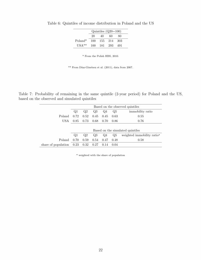
Table 6: Quintiles of income distribution in Poland and the US
Quintiles (Q20=100)
20 40 60 80
Poland* 100 155 214 303
USA** 100 181 293 491
* From the Polish HBS, 2010.
** From Dıaz-Gimenez et al. (2011), data from 2007.
Table 7: Probability of remaining in the same quintile (2-year period) for Poland and the US,based on the observed and simulated quintiles
Based on the observed quintiles
Q1 Q2 Q3 Q4 Q5 immobility ratio
Poland 0.72 0.52 0.45 0.45 0.63 0.55
USA 0.85 0.73 0.68 0.70 0.86 0.76
Based on the simulated quintiles
Q1 Q2 Q3 Q4 Q5 weighted immobility ratio*
Poland 0.70 0.59 0.54 0.47 0.48 0.58
share of population 0.23 0.32 0.27 0.14 0.04
* weighted with the share of population
22
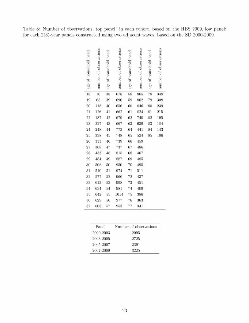
Table 8: Number of observations, top panel: in each cohort, based on the HBS 2009, low panel:for each 2(3)-year panels constructed using two adjacent waves, based on the SD 2000-2009.
age
ofhou
sehol
dhea
d
nu
mb
erof
obse
rvat
ions
age
ofhou
sehol
dhea
d
nu
mb
erof
obse
rvat
ions
age
ofhou
sehol
dhea
d
nu
mb
erof
obse
rvati
ons
age
ofhou
sehol
dhea
d
nu
mb
erof
obse
rvat
ions
18 10 38 678 58 865 78 348
19 65 39 690 59 862 79 308
20 118 40 656 60 846 80 239
21 126 41 662 61 824 81 215
22 187 42 679 62 740 82 195
23 227 43 667 63 639 83 184
24 248 44 773 64 441 84 143
25 338 45 748 65 524 85 106
26 333 46 739 66 459
27 368 47 737 67 486
28 433 48 815 68 467
29 484 49 887 69 485
30 508 50 950 70 495
31 510 51 974 71 511
32 577 52 966 72 437
33 613 53 998 73 451
34 634 54 981 74 409
35 642 55 1014 75 386
36 629 56 977 76 363
37 608 57 953 77 341
Panel Number of observations
2000-2003 2095
2003-2005 2725
2005-2007 2391
2007-2009 3225
23
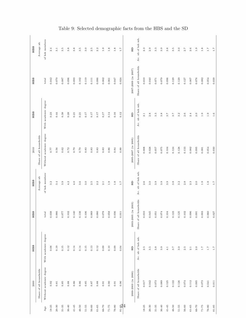
Table 9: Selected demographic facts from the HBS and the SD2000
HBS
HBS
HBS
2010
HBS
HBS
HBS
Share
ofall
house
hold
sAvera
genb
Share
ofall
house
hold
sAvera
genb
Age
Withoutacademic
degre
eW
ith
academic
degre
eto
tal
ofhsh
members
Withoutacademic
degre
eW
ith
academic
degre
eto
tal
ofhsh
members
18-2
50.92
0.08
0.038
3.2
0.77
0.23
0.042
2.4
26-3
00.81
0.19
0.066
3.4
0.56
0.44
0.070
3.1
31-3
50.85
0.15
0.077
3.9
0.62
0.38
0.087
3.5
36-4
00.88
0.12
0.102
4.2
0.72
0.28
0.096
3.8
41-4
50.86
0.14
0.140
4.0
0.79
0.21
0.093
3.8
46-5
00.86
0.14
0.138
3.6
0.79
0.21
0.102
3.5
51-5
50.85
0.15
0.106
3.0
0.83
0.17
0.119
3.0
56-6
00.87
0.13
0.069
2.5
0.83
0.17
0.111
2.5
61-6
50.88
0.12
0.080
2.2
0.83
0.17
0.086
2.2
66-7
00.91
0.09
0.078
2.1
0.83
0,17
0.062
1.9
71-7
50.90
0.10
0.058
1.9
0.86
0.14
0.061
1.8
76-8
00.91
0.09
0.036
1.8
0.84
0.16
0.047
1.8
81-8
50.96
0.04
0.011
1.7
0.88
0.12
0.024
1.7
2000-2
003
(in
2000)
SD
2003-2
005
(in
2003)
SD
2005-2
007
(in
2005)
SD
2007-2
009
(in
2007)
SD
Share
ofall
house
hold
sAv.nb
ofhsh
mb.
Share
ofall
house
hold
sAv.nb
ofhsh
mb.
Share
ofall
house
hold
sAv.nb
ofhsh
mb.
Share
ofall
house
hold
sAv.nb
ofhsh
mb.
18-2
50.017
2.5
0.010
2.6
0.008
2.1
0.010
2.3
26-3
00.042
3.5
0.045
3.0
0.028
2.8
0.040
2.9
31-3
50.073
3.8
0.051
3.9
0.057
3.3
0.071
3.3
36-4
00.089
3.9
0.074
3.9
0.075
3.8
0.079
3.9
41-4
50.125
4.1
0.104
3.9
0.104
3.7
0.096
3.8
46-5
00.122
3.7
0.123
3.8
0.124
3.7
0.129
3.5
51-5
50.126
3.0
0.125
3.2
0.128
3.2
0.129
3.0
56-6
00.074
2.5
0.102
2.8
0.133
2.6
0.127
2.7
61-6
50.112
2.1
0.096
2.3
0.082
2.4
0.067
2.6
66-7
00.095
2.0
0.091
2.0
0.095
2.0
0.076
1.9
71-7
50.073
1.7
0.093
1.9
0.081
1.9
0.082
1.8
76-8
00.041
1.7
0.060
1.8
0.054
1.9
0.054
1.7
81-8
50.011
1.7
0.027
1.7
0.030
1.6
0.039
1.7
24
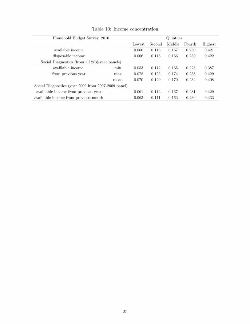
Table 10: Income concentration
Household Budget Survey, 2010 Quintiles
Lowest Second Middle Fourth Highest
available income 0.066 0.116 0.167 0.230 0.421
disposable income 0.066 0.116 0.166 0.230 0.422
Social Diagnostics (from all 2(3)-year panels)
avalilable income min 0.053 0.112 0.165 0.228 0.387
from previous year max 0.078 0.125 0.174 0.238 0.429
mean 0.070 0.120 0.170 0.232 0.408
Social Diagnostics (year 2009 from 2007-2009 panel)
avalilable income from previous year 0.061 0.112 0.167 0.231 0.429
avalilable income from previous month 0.063 0.111 0.163 0.230 0.433
25
6 Data appendix
Here I present the data from two major sources used in this paper. The first one is the HBS. Everyyear the Polish Central Statistical Office (CSO) publishes a report “Household Budget Surveys”,which contains the main descriptive statistics and indicators calculated on the basis of the HBS,with methodological notes explaining i.a. how the survey is conducted. This report is publiclyavailable on the CSO official website. Therefore, in this appendix I discuss only those HBS statisticswhich are crucial to the life cycle analysis. The second database is the Social Diagnostics, whichis publicly available and can be downloaded from the website (see www.diagnoza.com). Since thedata from this source were used in this study only to a limited extent, I also limit their discussionto the most important characteristics.
The HBS is conducted every year on a sample of around 37 thousand of Polish households. Itcollects households’ monthly income and spending data, as well as a number of other socio-economiccharacteristics. In the HBS, several measures of income are reported. The major income statisticsis the available income, which comprises total monthly net income form hired work, private farm oragriculture, other self-employment and free profession, from property, rental of a property or land,social insurance benefits, other social benefits and other income (including gifts and alimonies). Theother income measure, disposable income, is defined as available income less expenditures on non-consumption goods and services (for example expenditures on gifts donated to other households orsome taxes). In order to ensure comparability between the HBS and the SD, I use available income,but this measure does not differ significantly from disposable income. To construct consumptionprofiles, total monthly expenditures on consumer goods and services are used. This measure ofconsumption includes neither changes nor flows from capital (especially housing) wealth.
In order to eliminate the seasonality in the data, it would be optimal to have income and con-sumption reported on annual basis. However, only monthly data are available and therefore thoseare used in this study. Monthly frequency of data should not affect the estimated means of incomeand consumption distributions, but one should keep in mind that the estimates of the variancesare most probably overestimated.
Roughly 37 thousand of observations from the HBS spread unevenly over the households withdifferent age of household head, in line with the structure of the population. Therefore, cohortsused to calculate the mean and the variance of income / consumption distribution vary considerablyin size. The top panel of Table 8 presents the number of observations in such cohorts for year 2009.For each age of household head, there are between 10 and more than 1000 observations, with theaverage number of 544.
The second part of this study relies on all adjacent waves from the SD 2000-2009. Therefore,the size of the panels used to construct the transition matrices varies between 2000 and 3300observations (for exact numbers, see low panel of Table 8). In the SD, two major measures ofincome are reported: average monthly income from the previous year and monthly income fromthe last month. To avoid seasonality issues, I use the former.
The life cycle characteristics of the data such as the distribution of population according the ageof household head and the average number of households slightly differ between the two datasets(see Table 9). For instance, young households are underrepresented in the SD, while the share ofelderly individuals is greater than in the HBS.
Finally, these two databases are compared in terms of income concentration. Based on the HBSfrom 2000-2010, the shares of total households’ income in each quintile of population (where house-holds in a sample are ranked according to their available income) remained quite stable over time.
26

20 percent of the richest generate more than 40 percent of total households’ income, while thepoorest 20 percent have at their disposal only less than 7 percent of income (see Table 10). Thisresult remains unchanged when disposable rather than available income is used. Less precise es-timates are obtained from different panels from the SD, probably due to the smaller number ofobservations and relatively lower quality of data. Nevertheless, no clear discrepancy in terms ofincome concentration is observed between the HBS and the SD.
27