Working Paper WP 2016-353

Project #: UM16-13

Consumption Smoothing During the Financial Crisis: The Effect of Unemployment on Household Spending

Michael Hurd and Susann Rohwedder

Consumption Smoothing During the Financial Crisis: The Effect of Unemployment on Household Spending

Michael Hurd RAND, NBER, NETSPAR, and SMU

Susann Rohwedder RAND, NETSPAR, and SMU

October 2016

Michigan Retirement Research Center University of Michigan

P.O. Box 1248 Ann Arbor, MI 48104

www.mrrc.isr.umich.edu (734) 615-0422

Acknowledgements The research reported herein was performed pursuant to a grant from the U.S. Social Security Administration (SSA) funded as part of the Retirement Research Consortium through the University of Michigan Retirement Research Center Award RRC08098401. The opinions and conclusions expressed are solely those of the author(s) and do not represent the opinions or policy of SSA or any agency of the federal government. Neither the United States government nor any agency thereof, nor any of their employees, makes any warranty, express or implied, or assumes any legal liability or responsibility for the accuracy, completeness, or usefulness of the contents of this report. Reference herein to any specific commercial product, process or service by trade name, trademark, manufacturer, or otherwise does not necessarily constitute or imply endorsement, recommendation or favoring by the United States government or any agency thereof.

Regents of the University of Michigan Michael J. Behm, Grand Blanc; Mark J. Bernstein, Ann Arbor; Laurence B. Deitch, Bloomfield Hills; Shauna Ryder Diggs, Grosse Pointe; Denise Ilitch, Bingham Farms; Andrea Fischer Newman, Ann Arbor; Andrew C. Richner, Grosse Pointe Park; Katherine E. White, Ann Arbor; Mark S. Schlissel, ex officio

Consumption Smoothing During the Financial Crisis: The Effect of Unemployment on Household Spending

Abstract

Because of data limitations, the quantification of consumption smoothing in response to economic shocks has been challenging to investigate empirically. We used monthly data on total household spending, income, and labor force participation to estimate the effects of unemployment on household spending. The data come from the RAND American Life Panel, a standing survey sample that is representative of the United States adult population. We compare monthly spending and income of households prior to unemployment with spending and income following unemployment for up to 40 months. We compare spending and income following re-employment with spending and income while unemployed. We find that by month two of unemployment total household spending per month declined to about 83 percent of pre-unemployment spending. At about 14 months of unemployment, spending began to decline further, reaching 70 percent of pre-unemployment spending by month 30. Income declined much more sharply to 37 percent of its pre-unemployment level by month two of unemployment, with little change after that as the duration of unemployment increased. Thus, consumption does not decline as much as income, so that it is somewhat smoothed relative to income; yet, particularly over long-duration unemployment the decline is substantial.

On re-employment, income increased rapidly, spending much less rapidly. As of the third month, high-frequency spending was about 9 percent above its value in the last month of unemployment. It continued to increase until it was about 20 percent higher. Just as with an income drop, spending is somewhat smoothed when income increases.

Citation

Hurd, Michael, and Susann Rohwedder. 2016. “Consumption Smoothing During the Financial Crisis: The Effect of Unemployment on Household Spending.” Ann Arbor, MI. University of Michigan Retirement Research Center (MRRC) Working Paper, WP 2016-353. http://www.mrrc.isr.umich.edu/publications/papers/pdf/wp353.pdf

Authors’ acknowledgements

This research was supported by a grant from the Social Security Administration via the Michigan Retirement Research Center (UM16-13) and the National Institute on Aging (grant R01AG035010). Joanna Carroll provided excellent programming assistance. The ALP Financial Crisis Survey data used in this paper were collected with support from various grants from the National Institute on Aging (R01AG020717, P01AG022481, R01AG035010, P01AG026571 and P30AG012815) and from the Social Security Administration.

1

Introduction

The Great Recession officially started in December 2007 and ended in June 2009.

However, the economic situation of many households did not improve thereafter, and in many

cases it worsened. The national unemployment rate continued to go up, reaching its peak of

10.0 percent in October 2009 and remaining over 9.0 percent until October 2011. Besides

these labor market challenges, households also experienced economic shocks in the housing

and stock markets. Many households responded to the recession by reducing consumption

(spending): in the RAND American Life Panel (ALP) about 75 percent of households reported

reducing spending because of the financial crisis in the months following the collapse of the

stock market. That gives a sense of the wide distribution of effects, but the size of these effects

is also of great interest to both economists and policy makers. The magnitude of the reduction

would convey the extent to which households are able to smooth their consumption and

maintain their economic well-being when experiencing economic shocks. A marked reduction

in consumption, accompanied by an inability to smooth it, could contribute to further

contractions in the overall economy, leading to a downward spiral in United States economic

activity.

According to economic theory, the size of the consumption response to a shock depends

on the degree to which households are insured against such shocks, and on whether the

economic shock is permanent. If shocks to income were fully insured, then households would

be able to smooth their consumption completely. Some types of insurance, such as

unemployment benefits, do not replace 100 percent of earnings. In the absence of complete

insurance, households need to find ways of buffering shocks. One possibility is self-insurance.

That is, assuming sufficient liquidity of assets, households could set aside some money in

2

healthier times in order to be able to smooth the effect of economic shocks. Households doing

so would be able to distribute the effect of the shock over a longer period of time, but would

still need to re-optimize their consumption if the shock proves permanent.

The ability of households to adjust their consumption is likely to vary by good or service.

For some categories of spending, an immediate adjustment in response to a shock may not be

possible. This is particularly true for spending on durable goods, such as automobiles or major

household appliances, where the consumption services are distributed over a longer period of

time, although payment tends to occur at the time of purchase. Even some nondurable

categories of spending, such as those purchased through a contract for communications or

insurance services, may be difficult to adjust quickly. Patterns of change observed in some sub-

categories of spending cannot be generalized to others.

The question of consumption smoothing in response to economic shocks is challenging

to investigate empirically for at least two reasons. First, it is difficult to find sizeable,

unanticipated changes in households’ economic circumstances. For example, in “normal” times

stock prices increase and decrease within modest ranges. Such modest changes may be

anticipated and not lead to spending changes. Second, there are very few U.S. data sources

that track total household spending. The Consumer Expenditure Survey (CEX) collects a

comprehensive set of measures of household spending, but while there is a short longitudinal

component, the CEX lacks detail on labor market activity.

Given the lack of comprehensive measures of household spending, several studies have

sought to explore smoothing of food expenditures, for which data are available. Using data

from the Health and Retirement Study (HRS) and the Panel Study of Income Dynamics (PSID),

Stephens (2004) found that unemployment was associated with a reduction of approximately

3

16 percent in food spending. More to the point, Gruber (1997) used food spending in the PSID

(1968-1987) to estimate the effect of public unemployment insurance (UI) benefits on

consumption smoothing. He found that those who received generous UI benefits experienced

little change in consumption during and after a period of unemployment. Those with no UI

benefits experienced a drastic reduction (approximately 22 percent) in consumption. UI

benefits thus seem to have a significant effect on consumption smoothing, especially among

those who do not anticipate the unemployment shock. There appeared to be no differential

long-term effects of unemployment on consumption by level of UI entitlement, but eligibility

for such benefits does seem to crowd out private savings that would otherwise buffer

unemployment shocks.

Using Canadian data that covered 1993 to 1995, Browning and Crossley (2009) derived a

fairly comprehensive measure of household spending, albeit in a sample limited to those who

experienced unemployment. Their empirical results suggest that among households with no

liquid assets, total household expenditure is sensitive to the level of unemployment benefits.

Among specific commodities, they found expenditures on clothing were more sensitive to cuts

in benefits than were expenditures on food.

In this paper we use monthly data on household spending, household income, and labor

force participation to estimate the effects of a specific economic shock — unemployment — on

household consumption. These data, collected through a high-frequency survey, allowed us to

compare changes in spending and income of households recently experiencing unemployment

with those in households where respondents continue to be employed. We estimated the time

trajectory of changes in spending and income by durations (as measured in months) of

unemployment. We calculate the implied elasticities of spending with respect to income. We

4

repeat such calculations following re-employment to find similar trajectories of income and

spending.

Data: The ALP Financial Crisis Surveys

The RAND American Life Panel

We collected data for this research through the RAND American Life Panel (ALP) survey.

The ALP is an ongoing Internet panel survey, operated and maintained by RAND Labor and

Population. In November 2008, at the time of our first survey, it comprised about 2,500

persons, and about 1,000 new panel members have been added since then. Panel members

were initially recruited from respondents to the University of Michigan Survey Research

Center’s Monthly Survey (MS). The MS is considered to have good population representation

(Curtin, Presser, and Singer, 2005). At the end of an MS interview, respondents are asked to

participate in the ALP; about 80 percent do so. ALP participants without Internet access were

initially provided a Web TV (www.webtv.com/pc/) account, Internet subscription, and an email

account (an approach used successfully for many years in the Dutch CentER panel and which

helps reduce selection bias against noncomputer-owners). Later ALP recruitment efforts

provided participants without Internet access with laptops. The ALP uses post-stratification

weights to approximate the distributions of respondent age, sex, ethnicity, education, and

income in the Current Population Survey.

Several times monthly, respondents received an email request that they visit the ALP

website to complete questionnaires that typically take no more than 30 minutes to finish.

Respondents were paid about $2 per three minutes of survey time. Response rates were

5

typically between 80 and 95 percent depending on the topic, the time of year, and how long a

survey is kept in the field.

The ALP had conducted a large number of longitudinal surveys of its respondents, so

that over time it has collected data on a very wide range of covariates. The ALP has asked

respondents about their financial knowledge and their retirement planning, as well as

hypothetical questions about risk aversion. The ALP has also administered to its respondents’

modules of the Health and Retirement Study (HRS), including the wide range of HRS health

queries and the HRS cognitive battery.

A strength of the ALP is its use of Internet technology. This allows for a short turn-

around time between questionnaire design and the fielding of a survey, facilitating rapid

responses to new events or insights. Thus, surveys can be operated at high frequency, reducing

risk of missing events or their effects on households.

The Financial Crisis Surveys

The very large stock market declines in October 2008 prompted the ALP’s first financial

crisis survey, administered in November 2008.1 The survey covered a broad range of topics,

including life satisfaction, self-reported health measures, indicators of affect, labor force status,

retirement expectations, recent or potential job loss, housing, financial help (received, given,

and expected), stock ownership and value (including recent losses), stock transactions (recent

and expected over the next six months), expectations about stock market returns (one year

ahead, 10 years ahead), spending changes, credit card balances and changes in amounts

carried, impact of the financial crisis on retirement savings, and expectations about asset

1 See Hurd and Rohwedder (2015) for a description of the financial crisis surveys, including response rates, survey length, fielding schedule, and other details.

6

accumulation. We administered a second interview to the same panel in late February 2009

covering approximately the same topics.

In our first survey, 73 percent of households reported they had reduced spending

because of the economic crisis. This reinforced our motivation for undertaking this study. Such

reductions can have welfare implications, increasing the importance of understanding their

magnitude. Obtaining better data on how spending responds to economic shocks can also help

establish the empirical connection between the triggering events and the magnitude of

consumption reductions. The reported wide-spread spending reductions prompted us to re-

orient the survey by expanding the collection of quantitative information on the components of

spending.

Beginning with the May 2009 interview (wave 3), we established a monthly interview

schedule to reduce the risk of recall error about spending and to collect data at high frequency

on items such as employment, satisfaction, mood, affect, and expectations. We also sought

detailed sequencing of events and their consequences.2

Measuring Spending

Each month we asked about spending in 25 categories during the previous month.

These high-frequency categories comprised about 70 percent of total spending. Every third

month, beginning in July 2009, we asked about spending during the previous three months on

an additional 11 low-frequency categories plus seven big-ticket items. Taken together, the

monthly and quarterly surveys measured total spending over a three-month period. This three-

2 To further reduce recall error, we made the survey available to respondents only for the first 10 days of each month (except when the first day of the month fell on a weekend). Thus stated variables such as unemployment refer to approximately the first 10 days of a month, not the entire month.

7

month schedule of two shorter monthly surveys and a longer quarterly survey continued

through financial crisis survey wave 32 (October 2011).

After wave 32, monthly surveys of high-frequency spending categories continued, but

every third month, half of the sample was randomly broken out to receive monthly surveys of

low-frequency categories during that quarter, with the intent of checking for recall error on

low-frequency items. For spending analyses of low-frequency categories in this paper, we used

only the quarterly totals. This schedule continued through wave 50 (April 2013). Then, the

surveys of low-frequency categories reverted to quarterly-only, and the surveys of spending on

what had been high-frequency items were also reduced to quarterly in frequency (though the

period of interest remained the preceding month). The last of the financial surveys was

conducted in wave 61 (January 2016). The survey schedule is summarized in Table 1.

These surveys are unique in several ways. The first and most obvious is that they are

monthly panel surveys. This design permits the observation of the immediate effects of

changes in the economic environment that cannot be captured in low-frequency surveys via

retrospection. Second, we are measuring the majority of total spending on a monthly basis.

This measurement reduces recall bias for high-frequency purchases. Yet, because the surveys

cover an entire year, this measurement also captures low-frequency purchases. The use of a

reconciliation screen in the consumption module, described in detail below, substantially

reduces noise in the spending data, allowing meaningful analysis even in a small sample. The

combination of spending data with a very rich set of covariates, elicited at high frequency,

allows for a wide variety of analyses, with much more thorough information on timing and

sequencing of events for investigating determinants and effects.

8

Eliciting Total Household Spending

The 25 categories queried in the monthly surveys are shown in Appendix Table 1,

grouped as they were displayed. For example, the following categories were displayed at the

same time because they are associated with household operations.

Mortgage Rent Electricity Water Heating fuel for the home Telephone, cable, Internet Car payments: interest and principal

The grouping by broad types of spending or by frequency of spending was meant to facilitate

placement of reported amounts in the proper category: The thought was that respondents

unsure about category placement might find it helpful to see other possibly relevant categories

simultaneously. Also, it was hoped that the grouping would reduce the risk of omission and

double-counting.

Appendix Table 2 shows the categories of spending elicited quarterly which we call “low

frequency spending.” The categories include durables, but also some nondurables purchased

irregularly or at low frequency.

A major innovation was the development of a “reconciliation” screen. Outliers are a

problem in self-administered data collection, such as Internet interviewing, because there is no

interviewer to question extreme values. Therefore, we designed a new strategy to help with

outliers in the ALP. Following the queries about spending on the 25 categories in the previous

month, we presented the respondent with a summary table listing the responses and summing

9

them to produce an implied monthly spending total. We invited the respondent to correct any

items after seeing this total.

This has had two very favorable results: It reduced item nonresponse to a low level, and

it reduced outliers, which can have a large impact on statistical standard errors. Appendix

Table 3 presents a display of the reconciliation screen. In the initial wave that elicited spending

(wave 3 of the financial crisis surveys), respondents modified or updated about 3 percent of

their entries after seeing the reconciliation screen. The rate of correction declined further to

about 2 percent by wave 9. Thus the typical person would correct one entry approximately

every other wave.

Although this seems like a small rate of correction, the effect on outliers can be

substantial if the corrections are for entries that are extreme. A measure of the potential

extent of the problem is the standard deviation of spending. While some fraction of the

measured standard deviation reflects true variation in spending across individuals, some

fraction is the result of measurement error and often is the result of extreme outliers. In the

first two waves the reduction in the standard deviation was very substantial: from an average

of $17,700 to $4,100. In later waves the reduction was much smaller. Still, averaged over 20

waves, the standard deviation was 64 percent higher before the reconciliation screen. This

reduction had a substantial effect on the standard errors in the estimation of models of

spending.

10

Comparison with the Consumer Expenditure Survey

As a check, we compared the annual spending reported in our panel survey with that in

the cross-sectional CEX, the most authoritative survey measure of spending at the household

level. We chose the calendar year 2010 for this comparison, as this was the first complete year

of monthly data on household spending in the ALP and was also the latest calendar year for

which published tables from the CEX are available. For ALP we calculated spending over a year

by summing all 25 monthly spending items from the 12 monthly surveys and the quarterly

reported spending items from the quarterly surveys covering 2010. Average spending in 2010

as reported in the CEX was $42,736.3 Average weighted spending in the ALP was quite close at

$41,360, or 97 percent of CEX spending. The same CEX-ALP comparison conducted for the 2011

data showed ALP spending at 98 percent of CEX spending.

Measurement of Income

We asked about income during the previous month. The respondent was queried about

any earnings, including those of a spouse, and the amount before taxes and other deductions.

We asked whether the household had any additional income sources in other broad categories

in the previous month, including income from investments such as dividends, interest, or rental

income; retirement income such as Social Security, pensions, or other annuities; and

government benefits such as unemployment, disability, SSI benefits, or other welfare benefits.

(In case of item nonresponse, we used bracketing.) We asked households with any of these

income sources the total amount from them before taxes and other deductions.

3 We report CEX totals excluding “personal insurance and pensions” as these may contain components of saving and are not collected in the ALP.

11

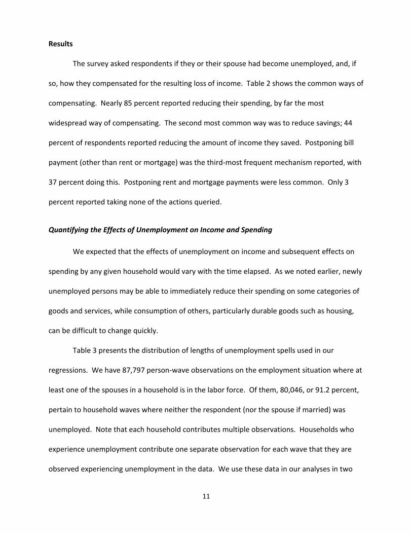
Results

The survey asked respondents if they or their spouse had become unemployed, and, if

so, how they compensated for the resulting loss of income. Table 2 shows the common ways of

compensating. Nearly 85 percent reported reducing their spending, by far the most

widespread way of compensating. The second most common way was to reduce savings; 44

percent of respondents reported reducing the amount of income they saved. Postponing bill

payment (other than rent or mortgage) was the third-most frequent mechanism reported, with

37 percent doing this. Postponing rent and mortgage payments were less common. Only 3

percent reported taking none of the actions queried.

Quantifying the Effects of Unemployment on Income and Spending

We expected that the effects of unemployment on income and subsequent effects on

spending by any given household would vary with the time elapsed. As we noted earlier, newly

unemployed persons may be able to immediately reduce their spending on some categories of

goods and services, while consumption of others, particularly durable goods such as housing,

can be difficult to change quickly.

Table 3 presents the distribution of lengths of unemployment spells used in our

regressions. We have 87,797 person-wave observations on the employment situation where at

least one of the spouses in a household is in the labor force. Of them, 80,046, or 91.2 percent,

pertain to household waves where neither the respondent (nor the spouse if married) was

unemployed. Note that each household contributes multiple observations. Households who

experience unemployment contribute one separate observation for each wave that they are

observed experiencing unemployment in the data. We use these data in our analyses in two

12

different ways. For the descriptive statistics we compute the difference in household income

and household spending between the month preceding the onset of unemployment and the

various months during unemployment. In the regressions we present fixed effects estimations

which incorporate covariates in the comparison of income and spending while unemployed

with income and spending while employed.

There were 1,618 spells of unemployment of at least one month, that is, monthly

observations on people who were unemployed following a month of employment. Some of the

1,618 returned to employment in the following month and some continued in unemployment

in the following month. There were 990 spells of unemployment that lasted at least two

months, and there were 681 spells that lasted at least three months, and so forth on to 301

spells of 20 to 24 months and 252 of 36 or more months. The data of someone with a spell that

lasts for many months will enter the estimations many times.

Figure 1 shows spending on high-frequency items before (pre) and during (post)

unemployment by month of unemployment spell among those with 12 or more months of

continuous unemployment. In the month when unemployment commences, spending is about

$2,300 compared with spending in the previous month of $2,500. Spending continues to

decline until about seven months of unemployment when it is $1,900 or 77 percent of its pre-

unemployment value (the top line). With continuing unemployment, spending continues at

about 75 percent of its pre-unemployment value.

Because the figure pertains to people who are unemployed for 12 months or more, pre-

unemployment income should not vary across durations of unemployment. This would be true

were the sample to be the same across durations, but that is not the case: Not everyone is

interviewed in every month so that the sample changes modestly in each month of

13

unemployment duration. For example, spending at month four is based on 160 observations.

These are people who became unemployed four months earlier and who were interviewed and

reported spending in both month four and prior to becoming unemployed. Furthermore, they

eventually were unemployed for 12 months or more. Spending at month five is based on 142

observations. They became unemployed five months earlier and were interviewed and

reported spending in both month five and prior to becoming unemployed. Most of them, but

not all, were interviewed and reported spending in wave four. Both pre-unemployment

spending and spending at month four are calculated over the 160 observations. Both pre-

unemployment spending and spending at month five are calculated over the 142 observations.

Despite the variation in sample, spending prior to unemployment is relatively flat.

A possible complication concerns expectations about eventual re-employment and its

effect on spending earlier in the spell of unemployment. For example, individuals who are

realistically less optimistic about finding a job should choose a sharper decline in spending even

months before re-employment than individuals who are realistically more optimistic. If

expectations have predictive power for unemployment duration, there should be a positive

relationship between spending reduction and unemployment duration. An implication is that

relative spending by month of unemployment should be calculated over observations that

eventually have the same duration of unemployment. We address that issue in Table 4.

The table shows the ratio of spending in a month when unemployed to spending prior

to unemployment, classified by the eventual duration of unemployment. If such ratios in a

particular month of unemployment vary negatively with eventual duration, that could be

regarded as evidence that the eventual duration of unemployment influences spending even

months before re-employment. For example, in row three (which shows log spending at month

14

three of unemployment relative to spending prior to unemployment), among those with

unemployment duration of three months or more (as shown by the column number), spending

was reduced in month three of unemployment (read down column three to row three) to 91.2

percent of pre-unemployment levels. Among those with unemployment duration of 12 months

or more, spending was reduced in month three to 86.8 percent of pre-unemployment levels.

This variation is consistent with the hypothesis that the duration of unemployment influences

spending declines even early in the unemployment spell. However, other rows do not show a

consistent decline and where there is a difference, it is relatively small. Under that

interpretation we concluded that we can aggregate observations according to their

unemployment state in any particular wave: We would not have to further disaggregate by the

eventual duration of unemployment.

Low-frequency Spending

As discussed above, the ALP Financial Crisis Survey included both monthly and quarterly

collection of data on household spending. The quarterly surveys, conducted in January, April,

July, and October, each covered expenditures in the preceding three months on a limited list of

spending categories, including automobiles and six other big-ticket items. Conducting part of

the financial surveys at lower frequencies had the advantages of limiting respondent burden

and survey costs. It had the drawback of reducing the number of observations of spending

changes. For example, among those with unemployment durations of 12 months or more, we

have about 56 observations on quarterly spending for each month of unemployment,

compared to about 150 observations of monthly spending on high-frequency items. Because of

the smaller sample sizes, we cannot present results for low-frequency items in a manner similar

15

to the presentation for high-frequency items in Figure 1. Instead, we present results that are

less dependent on a large sample.

Figure 2 shows the percentage ratio of two means: the mean of quarterly spending for

the month of unemployment and the mean of quarterly spending just prior to unemployment.

Thus, in the figure, the percentage ratio in month one of unemployment is 86 percent,

indicating a 14 percent drop since the preceding quarter. The percentage ratio then gradually

increases through the following months, before eventually declining by month six. Note that

quarterly spending pertaining to the first month of unemployment also partially reflects

spending from the two preceding months, months when the person was not yet unemployed.

Figure 3 is similar to Figure 2 except the analysis is based on medians instead of means.

Here, at one month of unemployment (calculated over everyone who had any unemployment

regardless of duration), quarterly spending is about 20 percent lower than the pre-

unemployment level. Although there appears to be estimation error due to small samples, the

overall impression is that, as measured by the ratio of medians, low frequency spending is

approximately constant with duration of unemployment at least up to eight months of

unemployment.

Low-frequency expenditures are a combination of durable and nondurable items

infrequently purchased. The spending trend shown in Figures 2 and 3 is consistent with a

cessation of durables purchases with the onset of unemployment, combined with a

continuation of low-frequency payments such as for taxes and insurance.

To smooth sampling and measurement errors, we used a local polynomial smoothed

regression of the deviation of spending in logs at unemployment duration t, minus the log of

spending just prior to unemployment, on indicator variables for duration, but where the

16

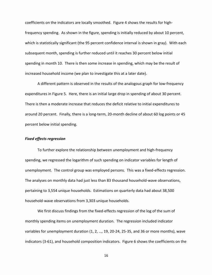
coefficients on the indicators are locally smoothed. Figure 4 shows the results for high-

frequency spending. As shown in the figure, spending is initially reduced by about 10 percent,

which is statistically significant (the 95 percent confidence interval is shown in gray). With each

subsequent month, spending is further reduced until it reaches 30 percent below initial

spending in month 10. There is then some increase in spending, which may be the result of

increased household income (we plan to investigate this at a later date).

A different pattern is observed in the results of the analogous graph for low-frequency

expenditures in Figure 5. Here, there is an initial large drop in spending of about 30 percent.

There is then a moderate increase that reduces the deficit relative to initial expenditures to

around 20 percent. Finally, there is a long-term, 20-month decline of about 60 log points or 45

percent below initial spending.

Fixed effects regression

To further explore the relationship between unemployment and high-frequency

spending, we regressed the logarithm of such spending on indicator variables for length of

unemployment. The control group was employed persons. This was a fixed-effects regression.

The analyses on monthly data had just less than 83 thousand household-wave observations,

pertaining to 3,554 unique households. Estimations on quarterly data had about 38,500

household-wave observations from 3,303 unique households.

We first discuss findings from the fixed-effects regression of the log of the sum of

monthly spending items on unemployment duration. The regression included indicator

variables for unemployment duration (1, 2, …, 19, 20-24, 25-35, and 36 or more months), wave

indicators (3-61), and household composition indicators. Figure 6 shows the coefficients on the

17

indicators for length of unemployment and the 95 percent confidence intervals (twice the

standard error on either side). Thus, high-frequency spending declined from pre-

unemployment spending by about 10 log points or 9 percent in the first month of

unemployment. In the second month, it declined by an additional seven log points to 16

percent below pre-unemployment spending. The rate of decline then slowed but nonetheless

continued. This continuing decline was somewhat obscured by error in the estimates but

showed clearly when we took a moving average of the coefficients (Figure 7). This shows that

the decline continued for very long durations of unemployment, even if at a slower pace,

reaching more than 20 percent of initial spending.

Because low-frequency expenditures were surveyed once every three months instead of

every month as with high-frequency spending, there were only about one-third as many

observations. For the high-frequency, fixed-effects regression there were 1,500 observations

with a duration of one month or more. For the low-frequency analysis there were just 659 (see

Table 5).

We estimated a fixed-effects regression similar to that described above, but for the log

of spending on low-frequency items elicited quarterly. Figure 8 shows the coefficients.

Spending initially declined by much more (about 20 percent) than was the case for high-

frequency spending. But there was no further decrease in spending with unemployment until

the latter reached a duration of 13 to 14 months of unemployment. For very long spells of

unemployment (more than two years), low-frequency spending fell by a total of more than 40

log points, or about 33 percent below pre-unemployment levels.

18

Income Results

We estimate the decline in income following unemployment with a similar fixed-effects

regression where the left-hand variable is the log of monthly income and the right-hand

variables at the same is in the fixed-effects regression of log spending. Figure 9 shows the

coefficients on the indicator variable for unemployment duration and the upper and lower 95

percent confidence intervals. In the first (partial) month of unemployment, we estimate a

decline of 64 log points in pre-unemployment income, which is a reduction of 47 percent. In

the next month, it declines by a further 16 percent of pre-unemployment income, at which

point income is just 37 percent of its initial level. Income remains at approximately that level,

with possibly an increase at month 12.

To visualize spending and income paths simultaneously, Figure 10 combines estimates

of spending and income paths from Figures 6 and 9. These show the patterns in the preceding

displays: A drop in spending during the first several months of unemployment, then a very slow

further decline, and a large, immediate drop in income, followed by a slow increase. It is likely

that the continued spending drop despite the slight recovery in income has to do with asset

spend down and the possible realization that the unemployment spell may last longer than had

been anticipated, thus the need to spend more defensively.

Elasticity: High-frequency Income and Spending Compared

The elasticity of spending with respect to income is the percent change in spending

divided by the percent change in income. According to the fixed-effects analysis, income

dropped in the first month by 47 percent (=(1-exp(-0.64)*100), and spending by 9 percent, so

the one-month elasticity was 0.19. Income in the second month was 71 percent below the pre-

19

unemployment level and spending was 15 percent below, implying an elasticity of 0.21. Figure

11 shows an upward trend in elasticity, reaching about 0.40 as unemployment approached

three years. The increase is due to slowly declining spending as the duration of unemployment

increases as shown in Figures 7 and 8. An increasing elasticity is consistent with depletion of

assets and with damped expectations of re-employment with the passing months of

unemployment.

Total Spending

Figure 12 combines the fixed-effects results from the high- and low-frequency patterns

of spending decline following unemployment. Initial spending in month zero is calculated as

the spending on high-frequency items in the month before unemployment ($2,452), and one-

third of the spending on low-frequency items in the quarter before unemployment ($1,108) for

a total of $3,560. The figure displays three trend lines—the simulated paths of high-frequency

spending (based on the fixed-effects coefficients displayed in Figure 6), of low-frequency

spending (based on the fixed-effects coefficients displayed in Figure 8) and of total spending by

month of unemployment, the sum of high- and low-frequency spending. The total declined

rapidly to about $2,981, then fluctuated at that level until week 30, when it fell more to about

$2,500 or about 70 percent of initial spending. By week 30, income was about 30 percent of

the initial value.

Re-employment

The time path of income and spending following the transition from unemployment to

employment is also of interest because spending should be smoothed when there is a positive

shock to income, not just a negative shock. For the analysis of re-employment, we used a fixed-

20

effects model with spending and income expressed as logarithms. Indicator variables were for

the number of months of employment following unemployment. We estimated separate

regressions for high- and low-frequency expenditures.

As illustrated in Figure 13, the log of income increased rapidly at employment. In the

first, partial month of employment, it was 60 log points above its level prior to re-employment.

By the third month, it was 1.15 log points above its prior value. Spending increased much less

rapidly: by the third month, high-frequency spending was just nine log points above its prior

value and continued to increase until it was about 20 log points higher. As employment

progressed, low-frequency spending increased more than high- frequency, probably because

during the unemployment phase, it fell more than high-frequency spending.

Conclusions

Using monthly and quarterly spending data, we found that total spending declined

within two months of the onset of unemployment to about 83 percent of its level prior to

unemployment. With some fluctuations, most likely due to small samples, it remained

approximately constant until unemployment duration of 30 months when it declined further,

reaching about 70 percent of its pre-unemployment level. An implication is that households

have some insurance against short-term unemployment through savings, an ability to borrow,

family support, or unemployment compensation, but they were not well insured against long-

term unemployment. The proximate cause of the longer-term reduction could be a liquidity

constraint: the exhaustion of savings or credit. But other mechanisms operating through

expectations could come into play: The long-term unemployed may have reduced their

expectations of the chances of re-employment or of the quality of the job on re-employment.

Either would cause a reduction in spending even among those without constrained liquidity.

21

Total spending is composed of spending measured at monthly intervals (high-frequency)

and spending measured at quarterly intervals (low-frequency). High frequency spending is

spending on nondurables; low frequency spending includes durables but some nondurables

that are purchased at irregular, low-frequency intervals such as property taxes, insurance,

home repairs, and trips and vacations. While both types decreased rapidly following the onset

of unemployment, high frequency spending stabilized at about 80 percent of pre-

unemployment spending whereas low frequency spending declined further, reaching just 57

percent of pre-unemployment spending.

The fact that spending decreases substantially more as unemployment becomes long

term suggests that there may be a need for better insurance against long-term unemployment,

possibly at the expense of short-term unemployment insurance. The logic would be that, in the

short term, households can finance spending (albeit with some reduction) from their own

resources but in the long term their resources are depleted. However, determining whether

this is so will require further study of the asset positions of households while they are

unemployed.

22

References

Browning, Martin and Thomas F. Crossley, 2009. “Shocks, Stocks and Socks: Smoothing Consumption over a Temporary Income Loss,” Journal of the European Economic Association, December 2009, 7(6):1169-1192.

Curtin R, S. Presser, and E. Singer (2005), “Changes in Telephone Survey Nonresponse over the Past Quarter Century.” Public Opinion Quarterly 69: 87-98.

Gruber, J. 1997. "The consumption smoothing benefits of unemployment insurance," The American Economic Review: 192-205.

Hurd, Michael D. and Susann Rohwedder, 2008. “Wealth Change and Active Saving at Older Ages,” presented at the January 2009 annual meetings of the American Economic Association, RAND typescript.

Hurd, Michael D. and Susann Rohwedder, 2010. “Consumption Smoothing during the Financial Crisis,” presented at the NBER Summer Institute Aging Workshop, July 2010.

Hurd, Michael D. and Susann Rohwedder, 2009. “Methodological Innovations in Collecting Spending Data: The HRS Consumption and Activities Mail Survey,” Fiscal Studies, 30(3/4), 435-459.

Hurd, Michael D. and Susann Rohwedder, 2015. "Measuring Total Household Spending in a Monthly Internet Survey: Evidence from the American Life Panel," in Improving the Measurement of Consumer Expenditures, eds. Christopher Carroll, Thomas Crossley and John Sabelhaus, University of Chicago Press, 2015, pp. 365-387.

Stephens Jr, Mel, 2004. "Job loss expectations, realizations, and household consumption behavior," Review of Economics and Statistics 86(1): 253-269.

23

Tables

Table 1

Month Year Wave High-frequency spending items Low-frequency spending items May … October

2009 … 2011

3 … 32

Monthly, asking about spending in last calendar month Quarterly, asking about spending

in last three calendar months

Nov … April

2011 … 2013

33 … 50

Monthly, asking about spending in last calendar month

Quarterly, asking about spending in last three calendar months, half of existing sample (assigned at random) Monthly, asking about spending last calendar month, half of existing sample (assigned at random) plus refresher sample

July … Jan

2013 … 2016

51 … 61

Quarterly, asking about spending in last calendar month

Quarterly, asking about spending in last three calendar months

Table 2: Compensating for Income Loss due to Unemployment

Way of compensating Percent Reduced spending 84.8 Reduced amount going into saving 43.4 Behind on mortgage 8.4 Behind on rent 15.2 Behind on other bills 37.3 None of the above 3.4

Note: Only queried of households where respondent or spouse lost a job resulting in a loss of income. Not asked of households where those losing a job immediately found a new one and suffered no loss of income.

24

Table 3: Number of unemployment spells by duration of spell

Month of unemployment N percent cumulative 0 80,046 91.17 91.17 1 1,618 1.84 93.01 2 990 1.13 94.14 3 681 0.78 94.92 4 581 0.66 95.58 5 438 0.5 96.08 6 356 0.41 96.48 7 336 0.38 96.87 8 283 0.32 97.19 9 232 0.26 97.45 10 221 0.25 97.7 11 194 0.22 97.93 12 161 0.18 98.11 13 164 0.19 98.3 14 136 0.15 98.45 15 114 0.13 98.58 16 109 0.12 98.7 17 95 0.11 98.81 18 88 0.1 98.91 19 80 0.09 99 20-24 301 0.34 99.35 25-35 321 0.37 99.71 36+ 252 0.29 100

87,797

25

Table 4: Spending following unemployment compared with pre-unemployment spending. Percent of pre-unemployment spending by month of unemployment and by minimum duration of unemployment

Minimum duration of unemployment

Months of unemployment 1 2 3 4 5 6 7 8 9 10 11 12

1 96.3 96.3 94.6 95.0 95.1 95.2 94.7 95.4 93.8 93.3 91.9 92.2

2 95.3 93.7 92.3 92.8 93.2 90.1 90.2 85.6 84.9 85.5 84.1

3 91.2 91.4 91.5 92.0 88.7 88.8 89.7 87.9 87.5 86.8

4 87.6 87.1 85.9 85.2 84.0 82.6 82.4 86.4 85.7

5 90.5 91.5 91.4 91.7 91.4 92.6 91.5 89.1

6 85.6 83.0 82.9 80.9 80.2 80.3 79.1

7 79.9 78.4 78.0 76.7 80.0 76.7

8 89.4 87.3 87.6 88.6 86.9

9 84.6 80.9 76.3 72.6

10 80.6 77.5 75.7

11 80.4 75.8

12 78.7

Note: each col umn sh ows th e spen ding ra tios by month of une mploy ment a mong t hose whose unemployment durations were equal to or greater than the column heading. The entries in a column show that the spending ratios decline with increasing unemployment. For example, among those with 12 or more months of unemployment spending in the first month of unemployment was 92.2 percent of spending prior to unemployment; that percentage declined to 78.7 percent in the 12th month of unemployment. The percentages in column 12 are derived from the data presented in Figure 1.

26

Table 5: Distribution of observations by length of unemployment. Low-frequency spending.

Length of unemployment (months)

N Percent

0 35,158 91.26 1 659 1.71 2 462 1.20 3 259 0.67 4 247 0.64 5 213 0.55 6 120 0.31 7 139 0.36 8 148 0.38 9 & 10 170 0.44 11 &12 145 0.38 13 &14 132 0.34 15 & 16 95 0.25 17 -19 105 0.27 20 - 24 128 0.33 25 - 29 99 0.26 30 - 39 102 0.26 40 or more

144 0.37

27

Figures

Figure 1: Spending on high-frequency items before (pre) and during (post) unemployment by month of unemployment spell among those with 12 or more months of continuous unemployment

Figure 2: Quarterly spending on low-frequency items following unemployment relative to quarterly spending prior to unemployment. Ratio of means.

0

500

1,000

1,500

2,000

2,500

3,000

1 2 3 4 5 6 7 8 9 10 11 12

Pre

Post

0

20

40

60

80

100

120

1 2 3 4 5 6 7 8Month of unemployment

Percentage of pre-unemployment spending: means

28

Figure 3: Quarterly spending on low-frequency items following unemployment relative to quarterly spending prior to unemployment. Ratio of medians.

Figure 4: Spending while unemployed relative to spending prior to unemployment: high-frequency items. Kernel smoothed trajectory.

0

20

40

60

80

100

120

1 2 3 4 5 6 7 8Month of unemployment

Percentage of pre-unemployment spending: medians -.6

-.4-.2

0C

hang

e in

log

spen

ding

sin

ce o

nset

of u

nem

p.

0 1 2 3 4 5 6 7 8 9 10 11 12 13 14 15 16 17 18 19 20number of months unemployed

95% CI lpoly smooth: ln(prior_mspend) - ln(mspend)

29

Figure 5: Spending while unemployed relative to spending prior to unemployment: low-frequency items. Kernel smoothed trajectory.

Figure 6: Regression coefficients: regression of log of the sum of monthly spending items (high-frequency) on unemployment duration indicators.

-1-.8

-.6-.4

-.20

Cha

nge

in lo

g sp

endi

ng s

ince

ons

et o

f une

mp.

0 1 2 3 4 5 6 7 8 9 10 11 12 13 14 15 16 17 18 19 20number of months unemployed

95% CI lpoly smooth: ln(prior_qspend) - ln(qspend)

-0.4

-0.35

-0.3

-0.25

-0.2

-0.15

-0.1

-0.05

0

1 2 3 4 5 6 7 8 9 10 11 12 13 14 15 16 17 18 1920

-22

23-2

526

-29

30-3

536

+

30

Figure 7: Moving average of regression coefficients: regression of the log of the sum of monthly spending items on unemployment duration indicators.

Note: Weights on regression coefficients centered at t are 0.1, 0.2, 0.4, 0.2, 0.1

Figure 8: Regression coefficients: regression of log of the sum of quarterly spending items (low-frequency) on unemployment duration indicators.

-0.3

-0.25

-0.2

-0.15

-0.1

-0.05

01 2 3 4 5 6 7 8 9 10 11 12 13 14 15 16 17 18 19

20-2

223

-25

26-2

930

-35

36 +

-1.2

-1

-0.8

-0.6

-0.4

-0.2

0

0.2

31

Figure 9: Regression coefficients: Log household monthly income following unemployment relative to pre-unemployment log income

Figure 10: Coefficients on log spending and on log income from fixed effects regression

-2

-1.8

-1.6

-1.4

-1.2

-1

-0.8

-0.6

-0.4

-0.2

01 2 3 4 5 6 7 8 9 10 11 12 13 14 15 16 17 18 19

20-2

223

-25

26-2

930

-35

36 o

r mor

e

-1.8

-1.6

-1.4

-1.2

-1

-0.8

-0.6

-0.4

-0.2

0

income

spending

32

Figure 11: Elasticity of spending with respect to income

Figure 12: Simulated path of total, high frequency and low frequency by month of unemployment following initiation

0

0.05

0.1

0.15

0.2

0.25

0.3

0.35

0.4

0.45

1 2 3 4 5 6 7 8 9 10 11 12 13 14 15 16 17 18 1920

-22

23-2

526

-29

30-3

536

or m

ore

0

500

1000

1500

2000

2500

3000

3500

4000

0 2 4 6 8 10 12 14 16 18 20 22 24 26 28 30 32 34 36 38 40

High Freq

Low Freq

Total

33

Figure 13: Log income and log spending (high frequency and low frequency) following re-employment relative to log income and log spending prior to re-employment

0

0.2

0.4

0.6

0.8

1

1.2

1.4

1.6

1 2 3 4 5 6 7 8 9 10 11

High frequency

Low frequency

income

34

Appendix

Construction of Unemployment Spells

The spells are mainly based on monthly observations of employment status. The

respondent reports about own employment status (work for pay; unemployed, looking for

work; temporarily laid off; on sick or other leave; disabled; retired; homemaker; self-employed;

student; other). Based on this information we determine for each wave whether the

respondent was working for pay or unemployed and looking for work. If the respondent is

working for pay then the variable measuring the length of the unemployment spell is set to

zero. In the first month of unemployment it is assigned the value one and the value two in the

second month of unemployment. If the respondent is observed working again then the length

of unemployment for that wave is set to zero again. Should there be a gap between waves, say,

because a respondent missed a wave or more, we developed an algorithm to fill these gaps

with additional information. First, if the gap is only one or two months and the person is

observed still being unemployed two months later, then we assume that this person was

continuously unemployed. If the person is working again two months later, then we do not

know when the unemployment ended, so we leave the measure of length of unemployment

missing and hope to fill this gap in the next step.

The second source of information comes from periodic modules that ask respondents

about the dates of unemployment spells. Because this information is recalled over the last 12

months for most respondents, but for some respondents over longer periods of time, we need

35

to be mindful of potential recall error in this retrospective reports.4 Therefore, we give priority

to the reported current employment status recorded in each wave and only use the dates to fill

remaining gaps that arise mostly because a respondent may not have participated in some

survey waves. When the survey frequency changes to quarterly in the latter part of the field

period we also use the retrospective information on unemployment spell dates to fill the gaps

of the intervening months between survey waves.

For married respondents we also asked every month about the employment status of

the spouse and unemployment spell dates of the spouse in occasional modules. So we have the

same information as for the respondent and construct unemployment spell data for the spouse

using the same algorithm described for the respondent.

Because spending (and income) is a household-level measure and is presumably

affected when either the respondent or the spouse (or both) are unemployed, we then

combine the information of unemployment spells of the respondent and spouse to a

household-level variable: If neither is unemployed and at least one is working for pay, then the

length of unemployment measure is set to zero. If one of the two is unemployed, then the

length of unemployment for the household takes the value of the unemployed person in the

couple. If both should be unemployed, which is very rare in our data, then the length of

unemployment of the household is set equal to the higher one of the individual spouse’s

measures of length of unemployment. For example, consider the situation where the

respondent becomes unemployed, then the length of unemployment takes the value one. As

long as the spouse’s employment status does not change to “unemployed” the count of

4 For many respondents we have overlapping reports from modules that are a year apart, but cover some of the same unemployment spells. From comparing the dates it is clear that there is reporting error in the reported dates.

36

“number of months of unemployment for the household continues counting the number of

months of unemployment of the respondent. Should the spouse become unemployed

eventually as well, then the length of unemployment still counts the length of the respondent’s

unemployment. It turns out that we only have 85 observations out of more than 80,000

person-wave observations where this happens.

Periods of self-employment of either spouse are excluded and the individual length of

unemployment variables are assigned a special missing code. These observations will not enter

the analyses.

37

Appendix Table 1: Items queried each month, grouped by actual screen display Screen 1:

Mortgage Rent Electricity Water Heating fuel for the home Telephone, cable, Internet Car payments: interest and principal

Screen 2:

Food and beverages Dining and/or drinking out Gasoline

Screen 3:

Housekeeping supplies Housekeeping, dry cleaning, and laundry services Gardening and yard supplies Gardening and yard services

Screen 4:

Clothing and apparel Personal care products and services Prescription and nonprescription medications Health care services Medical supplies

Screen 5:

Tickets to movies, sporting events, performing arts, etc. Sports, including gym and exercise equipment such as bicycles, skis, and boats Hobbies and leisure equipment

38

Screen 6:

Personal services, including cost of care for elderly and/or children, after-school activities Education, including tuition, room and board, books, and supplies Other child-related spending, not yet reported, including toys, gear, and equipment

Appendix Table 2: Additional 11 items queried quarterly beginning in the July survey about spending over previous three months Screen 1:

Big ticket items

• Automobile or truck • Refrigerator • Stove and/or oven • Washing machine and/or dryer • Dishwasher • Television • Computer

Follow-up questions on big ticket items queried amounts, and in the case of cars how the purchase was financed.

Screen 2:

Homeowner’s or renter’s insurance Property taxes Vehicle insurance Vehicle maintenance: parts, repairs, etc. Health insurance

Screen 3:

Trips and vacations Home repair and maintenance materials Home repair and maintenance services Contributions to religious, educational, charitable, or political organizations Cash or gifts to family and friends outside the household

39

Appendix Table 3: Selected Screen Shots from ALP Spending Module

Sample screen shot from the monthly spending survey module

40

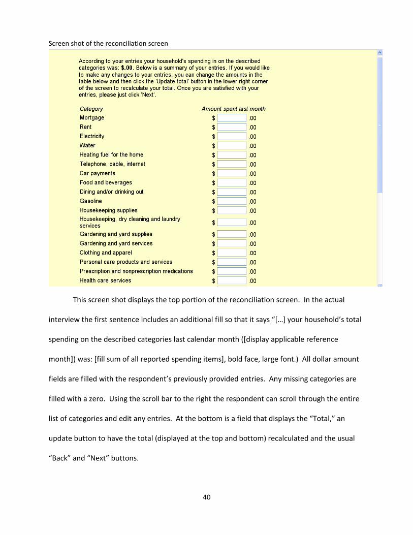
Screen shot of the reconciliation screen

This screen shot displays the top portion of the reconciliation screen. In the actual

interview the first sentence includes an additional fill so that it says “[…] your household’s total

spending on the described categories last calendar month ([display applicable reference

month]) was: [fill sum of all reported spending items], bold face, large font.) All dollar amount

fields are filled with the respondent’s previously provided entries. Any missing categories are

filled with a zero. Using the scroll bar to the right the respondent can scroll through the entire

list of categories and edit any entries. At the bottom is a field that displays the “Total,” an

update button to have the total (displayed at the top and bottom) recalculated and the usual

“Back” and “Next” buttons.