container liner-shipping network design using a path ... · pdf filecontainer liner-shipping...
TRANSCRIPT

Container liner-shipping network design using a path
formulation model for Indonesia
Hakan Kalem
Master ThesisErasmus University RotterdamErasmus School of Economics
Econometrics & Management ScienceOperations Research and Quantitative Logistics
Student number: 294925
Supervisor: R. DekkerCo-reader: J. Mulder
August 18, 2015

Dedicated to Emin Hamza and Esma.
1

Contents
1 Introduction 5
2 Problem definition 6
3 Literature 73.1 Strategic level . . . . . . . . . . . . . . . . . . . . . . . . . . . . . . . . . . . . 7
3.1.1 Network design . . . . . . . . . . . . . . . . . . . . . . . . . . . . . . . 73.1.2 Feeder network design . . . . . . . . . . . . . . . . . . . . . . . . . . . 83.1.3 Ship routes without transhipment . . . . . . . . . . . . . . . . . . . . 83.1.4 Hub-and-spoke network . . . . . . . . . . . . . . . . . . . . . . . . . . 93.1.5 General liner shipping network design . . . . . . . . . . . . . . . . . . 93.1.6 Route generation . . . . . . . . . . . . . . . . . . . . . . . . . . . . . . 9
3.2 Tactical level . . . . . . . . . . . . . . . . . . . . . . . . . . . . . . . . . . . . 103.2.1 Frequency determination . . . . . . . . . . . . . . . . . . . . . . . . . 103.2.2 Fleet deployment . . . . . . . . . . . . . . . . . . . . . . . . . . . . . . 103.2.3 Ship sailing speed optimisation . . . . . . . . . . . . . . . . . . . . . . 10
3.3 Operational level . . . . . . . . . . . . . . . . . . . . . . . . . . . . . . . . . . 103.3.1 Cargo routing . . . . . . . . . . . . . . . . . . . . . . . . . . . . . . . . 11
3.4 Cost estimations . . . . . . . . . . . . . . . . . . . . . . . . . . . . . . . . . . 123.5 Conclusion . . . . . . . . . . . . . . . . . . . . . . . . . . . . . . . . . . . . . 12
4 Solution approach 134.1 Mathematical model . . . . . . . . . . . . . . . . . . . . . . . . . . . . . . . . 13
4.1.1 Path Formulation Model (PFM) with routes . . . . . . . . . . . . . . 134.1.2 Extension 1: Multiple ships . . . . . . . . . . . . . . . . . . . . . . . . 164.1.3 Extension 2: Speed optimisation . . . . . . . . . . . . . . . . . . . . . 17
4.2 Route generation . . . . . . . . . . . . . . . . . . . . . . . . . . . . . . . . . . 174.2.1 Path construction . . . . . . . . . . . . . . . . . . . . . . . . . . . . . 184.2.2 Path construction with transhipment . . . . . . . . . . . . . . . . . . . 194.2.3 Filtering . . . . . . . . . . . . . . . . . . . . . . . . . . . . . . . . . . . 194.2.4 Contraint construction . . . . . . . . . . . . . . . . . . . . . . . . . . . 20
5 Data 225.1 Sources . . . . . . . . . . . . . . . . . . . . . . . . . . . . . . . . . . . . . . . 225.2 Requirements . . . . . . . . . . . . . . . . . . . . . . . . . . . . . . . . . . . . 22
5.2.1 Port list . . . . . . . . . . . . . . . . . . . . . . . . . . . . . . . . . . . 235.2.2 Fleets . . . . . . . . . . . . . . . . . . . . . . . . . . . . . . . . . . . . 24
2

5.2.3 Cargo demand . . . . . . . . . . . . . . . . . . . . . . . . . . . . . . . 255.2.4 Distance . . . . . . . . . . . . . . . . . . . . . . . . . . . . . . . . . . . 25
5.3 Preprocessing . . . . . . . . . . . . . . . . . . . . . . . . . . . . . . . . . . . . 255.3.1 Port aggregation . . . . . . . . . . . . . . . . . . . . . . . . . . . . . . 26
5.4 Parameter setting / Assumptions . . . . . . . . . . . . . . . . . . . . . . . . . 265.5 Technique . . . . . . . . . . . . . . . . . . . . . . . . . . . . . . . . . . . . . . 27
6 Results 286.1 Reference model . . . . . . . . . . . . . . . . . . . . . . . . . . . . . . . . . . 28
6.1.1 Difference between PFM and Reference model . . . . . . . . . . . . . 296.1.2 Reference* solution . . . . . . . . . . . . . . . . . . . . . . . . . . . . . 306.1.3 Reference*(ALL) solution . . . . . . . . . . . . . . . . . . . . . . . . . 30
6.2 Route generation . . . . . . . . . . . . . . . . . . . . . . . . . . . . . . . . . . 316.2.1 BASE solution . . . . . . . . . . . . . . . . . . . . . . . . . . . . . . . 336.2.2 Transhipment solution . . . . . . . . . . . . . . . . . . . . . . . . . . . 336.2.3 Extension 1: Multiple ships solution . . . . . . . . . . . . . . . . . . . 346.2.4 Extension 2: Speed optimisation solution . . . . . . . . . . . . . . . . 356.2.5 All settings combined solution . . . . . . . . . . . . . . . . . . . . . . 356.2.6 Custom input . . . . . . . . . . . . . . . . . . . . . . . . . . . . . . . . 36
6.3 Conclusion . . . . . . . . . . . . . . . . . . . . . . . . . . . . . . . . . . . . . 37
7 Conclusion 38
8 Discussion 40
9 Appendix 44
3

Summary
This thesis is conducted in order to improve the liner shipping network in the Indonesianports region. The network design problem is modelled with the use of a Path FormulationModel, which is a MIP. The model is primarily focused on the tactical and operational level,namely determining the allocation of cargo through different paths in the network. Pathsbelong to a route and consists of an origin and a destination port on which containers can betransported. As prerequisite, on the strategic level, routes are generated which serve as inputfor the PFM. The optimal solution maximises the profit by determining the set of paths tooperate and how much cargo each path transports. The solution consists of a set of routes tooperate. This model is further extended with transhipment, heterogeneous fleet, and speedoptimisation. The model is compared with a benchmark consisting of a network with six hubports. The results with all extensions show an improvement of the base solution by 12%.
4

Chapter 1
Introduction
In Indonesia there is unbalance in the domestic shipping trade between east and west partsof the country. Most shipping trade activity is in the region around Java, since this regionis more developed and most trade from outside Indonesia arrives there. While the outskirts(mainly east Indonesia) are less developed due to the large distance and low demand/supplyfrom these regions.
As a result the Indonesian government aims to improve the trade flows between east andwest Indonesia in order to improve the economic growth. Together with terminal opera-tors (Indonesia Port Corporation I-V), shipping companies and stakeholders, the Indonesiangovernment plans to improve the current situation. As a solution, pendulum routes are con-sidered to be used to connect east with west Indonesia. The characteristic of this kind ofroute is that the same ports (not all) are visited twice by going back and forth.
An important goal in this thesis is to develop a container shipping line network that willaccommodate balance in trade flows between east and west Indonesia. Certain aspects mustbe taken into account in determining such a network. Demand and supply of each port/regionis different, which requires the determination of what volume to transported to which portand by what order. Also, the current accessibility of ports requires the determination of whichtype of ships to use. Further, the availability of data determines the limitations of the model.Therefore, the data is required with regard to ports and its characteristics, possible ship fleet,costs and revenues structures.
This thesis starts by first defining the problem, which results in a main question and itssub questions. Based on these questions the literature is reviewed in order to acquire knowl-edge in the relevant field of research. Subsequently, a model is proposed to use for answeringthe main question. Before implementing the model, the available data is analysed in con-junction with the model requirements. This results in making simplification and assumptionto the model. Lastly, results are presented, conclusion are drawn, and future research andlimitations are discussed.
5
Chapter 2
Problem definition
In Indonesia there are many different kinds of ports with regard to attractiveness. That is,some ports are more profitable to serve than others. This causes unbalance in the shippingtrade across the country.
Our goal is to gain insight into the problem situation and conduct research whether thesituation at hand can be improved. Therefore, the aim is to build a model for the situationat hand and design container shipping network for liner shipping that improves the currentsituation.In designing such a network several issues must be taken into account. There are many lowdemand/supply ports in Indonesia which also have large distance from the central region(Java). This requires the determination of which ports to visit and in what order.Also the determination of which type of ship to operate is required. Since each ship type hasits own characteristics, e.g. capacity, speed and size.Based on this problem the main question is formulated as follows:
”Determine the best liner shipping network for Indonesian ports using a mathematicalmodel”
Based on the problem, the following research questions are formulated:
1. Which model can be used to design container shipping networks for liner shipping?
2. How can the model be adapted to the size of Indonesia ports region?
3. What data is needed and available to solve the model?
In order to determine which mathematical models can be used literature research is con-ducted in Chapter 3. Different models and relevant topics are discussed. In Chapter 4 amodel is proposed and the construction is discussed. Based on the model the data is analysedand prepared in order to run the model and compare it to a benchmark.
6

Chapter 3
Literature
In the literature the global shipping industry is divided into three modes of operation: indus-trial, tramp, and liner (Lawrence [1972]). The aim in industrial shipping is to minimise thetotal shipping cost over the owned ships. Tramp shipping refers to carriers that carries bulkcargo between specified ports according to a contract, which means cargo must be deliveredaccording to specified time frames. In liner shipping it must be decided which set of trips toserve and by what schedule by a carrier.
The relevant mode of operation for this research is liner shipping. Therefore, liner ship-ping is investigated further. In Meng et al. [2014] it is stated that the aim of liner containershipping network design is to determine which ports the ships should visit and in what order.For liner container shipping companies there are three decision-making levels: strategic, tac-tical, and operational (Pesenti [1995]). Long-term decisions are made at the strategic levelsuch as ship fleet size and mix, alliance strategies, and network design. Every three to sixmonths, based on the change in demand, decisions are made at the tactical level. Here, theliner shipping company needs to decide on the frequency of its services, allocation of shipsto routes, the sailing speed of those ships, and design schedules. At the operational level,decisions are made about whether to accept or reject cargoes, how to route accepted cargoes,and how to reroute or reschedule ships to cope with unexpected incidents.
In Meng et al. [2014] an overview and summary is given of the three decision-making levels.Based on this, in the following sections, the literature review is divided into these three levels.
3.1 Strategic level
Strategic Alliance and Fleet design and Mix, as discussed in Meng et al. [2014], are decisionmaking problems on the strategic level. However, these are assumed to be given a priori andare not discussed. While the Network design problem, also on the strategic level, is relevantfor this research and is discussed in the next section (3.1.1).
3.1.1 Network design
The liner container shipping network design problem is NP-hard (Agarwal and Ergun [2008]).Generally research on this topic can be classified into the following four categories (Meng
7
et al. [2014]): 1) Feeder network design, 2) Ship routes without transhipment, 3) Hub-and-spoke network, and 4) General liner shipping network design. In the following sections eachcategory is discussed in more detail.
3.1.2 Feeder network design
In this category a network divided into hub ports and feeder ports. Each feeder port eitheroriginates from or is destined to a hub port. There is also no transhipment within the feedernetwork.
In Fagerholt [1999] a set-partitioning model is proposed. In this model all possible routesare enumerated into single routes, i.e. routes that can be accomplished using the largestship. Then, the single routes that are not being used to its maximum potential are combinedinto feasible new routes. These routes are being operated by smaller ships. Finally, the set-partitioning model is used to determine which routes to use. The set of routes consists of thesingle routes and the combined routes. Later this model is extended in Fagerholt [2004] toenable the model to choose between multiple ships, where each ship has its own cost structure,capacity, and sailing speed.
In Sambracos et al. [2004] a meta-heuristic method is used for the VRP in order to de-sign a network with feeder ships and small containers from one depot port to 12 other ports.A List-Based Threshold Acceptance (LBTA) meta-heuristic method is used to minimise thetotal distance travelled and to determine the best sequence of ports to be visited. The LBTAis a stochastic method, which searches iteratively through the solution region.
3.1.3 Ship routes without transhipment
The aim in this category is to design one or a few liner service routes without containertranshipment.
Boffey et al. [1979] developed an interactive computer program and a heuristic optimisa-tion model for designing the ship route of a container ship. Each route was assigned a valuewhich is obtained by maximising the total freight revenue by use of a LP model.
In Lane et al. [1987] an analytical model is proposed. This model aims to plan for linercontainer shipping routes. First enumerate all possible ship routes and then choose theoptimal set of ship routes that satisfy the requirements by use of a set-partitioning model.
Rana and Vickson [1988] built a MINLP model for routing a single container ship. Byenumerating all possible round trips the model is linearised. As a result a MILP model iscreated and this is then solved using Benders’ decomposition technique. The model assumesthat the ships port-calling sequence is determined beforehand.
In Shintani et al. [2007] the assumption of port calling precedence relations is relaxed todesign a single ship route and empty container repositioning is considered. The problem wasformulated as a bilevel model, where the upper level was a knapsack problem choosing thebest set of calling ports, and given these ports the lower level identified the optimal callingsequence of ports. With a GA model problems were solved simultaneously. Chuang et al.[2010] proposed a fuzzy GA for designing a liner ship route by assuming that the containershipment demand was not a crisp number, but a fuzzy number.
8

3.1.4 Hub-and-spoke network
Imai et al. [2009] compared the efficiency of H&S networks and Multi Port Call (MPC)networks using a simple six-port example. In H&S one port in each service area is chosen asa hub, and the other four ports are connected by feeders. While in MPC, all six ports arevisited sequentially. They found that MPC network to be superior to the H&S network inmost scenarios. However, this might change based on the cost structure.
3.1.5 General liner shipping network design
In this category a network is designed which involves more ports in the network and allowsfor container transhipment operations.
For the liner shipping service network design problem with cargo routing, Agarwal and Ergun[2008] propose a multi commodity-based space-time network model. The model incorporatesa heterogeneous fleet, a weekly service frequency, multiple ship routes, and cargo tranship-ment. A MILP formulation is used with an exponential number of decision variables indicatingwhether a ship route is used or not. A greedy heuristic, a column generation-based algorithm,and a two-phase Benders’ decomposition-based algorithm is used. However, transhipment costwere not considered in the network design stage.
Alvarez extended the problem addressed by Agarwal and Ergun [2008] in two aspects.First, transhipment cost was explicitly incorporated into the network design. Secondly thedifferent ship types had different speed. By use of a combined tabu search and columngeneration-based heuristic to design the network.
Reinhardt and Pisinger [2012] presented a model with butterfly ship routes. This is aroute which contains a port that is visited twice and at which transhipment is allowed. Theirmodel also incorporates heterogeneous fleet and transhipment costs. An exact B&C algorithmto solve the problem.
In Mulder and Dekker [2013] a composite solution approach is used in which a LP is usedfor the Cargo Routing Problem (CRP). First the ports are aggregated into clusters and initialnetworks are created heuristically. After the initial solution the algorithm iterates throughCRP, speed optimisation, disaggration into feeder networks, and a GA to change networksuntil optimality is met. They are able to compute this for 58 ports.
In Brouer et al. [2014] the problem of Liner-Shipping Network Design (LSND) is discussedand they provide a general benchmark suite with data. They solve the benchmark suitewith a MIP model based on Alvarez with the extension to handle certain rotations andfrequencies. Further, a combined heuristic method is used with tabu search and heuristiccolumn generation.
3.1.6 Route generation
Fagerholt [2004] uses an algorithm to generate routes. It is an iterative algorithm which startswith small number of ports and extends by adding ports if the capacity constraints are notexceeded. In case the constraint is met, a TSP is solved to find the optimal visiting portsequence for the new route.
9

3.2 Tactical level
Meng et al. [2014] discuss the following studies in this category which are relevant for ourresearch, namely frequency determination, fleet deployment, ship sailing speed optimisation,and schedule design. Schedule design has a lower priority and therefore is neglected in thisthesis. In the following sections the other three topics are discussed separately.
3.2.1 Frequency determination
The time (in days) between two consecutive ships on a route visiting a port is called theservice frequency. Generally in the literature, a weekly frequency is used in order to maintaina steady service by liner shipping (Meng et al. [2014]). The distance travelled by a ship on aroute and its speed determines the number of ships required on a route.
3.2.2 Fleet deployment
Fleet deployment is about optimisation of assigning ships to routes. One of the relevanttopics in here is the calculation of the required ships on a route. In order to calculate howmany ships are required for a route, frequency of service and port waiting time are required.Wardana [2014] uses the following expression to calculate the number of ships required on aroute with weekly service frequency.
ns = d(ds
+ np)/7e (3.1)
Where ns number of ships required d is distance in nautical miles, s the speed in knots,and np the number of port visits. Note that for each port visit a port stay time of 24 hours isassumed. Also, distance denotes the total distance travelled by a ship on the route. Further,since an integer number is required, this number gets rounded up.
3.2.3 Ship sailing speed optimisation
Given the weekly service interval and the calculation of the number of ships, the speed of theship travelling can be altered in order to reduce the number of ships used by travelling faster,alternatively reduce the fuel cost by travelling slower.Based on Branch and Stopford [2013] and Alderton [2010] there is a general agreement thatbunker consumption can be estimated by the following function:
F (s) = (s/vF∗ )3fF∗ (3.2)
Where, s is any speed between min speed sFmin and max speed sFmax of the vessel F , vF∗ is thedesign speed, and fF∗ is the fuel consumption at design speed.
3.3 Operational level
In Meng et al. [2014] a number of operational-level decision problems in liner shipping isdiscussed, such as cargo booking, cargo routing ship rescheduling, and crew scheduling. Inthis thesis only cargo routing is considered relevant, therefore this is discussed next.
10

3.3.1 Cargo routing
Container routing problems are generally formulated as LP models where the number of con-tainers is treated as a continuous decision variable. Some studies have modelled containerrouting using O-D-based link flow formulations (e.g., Agarwal and Ergun [2008], Brouer et al.[2011]), origin-based link flow formulations (e.g., Alvarez, Wang and Meng [2012]), or segment-based formulations, where a segment is a sequence of consecutive links (e.g., Bell et al. [2011],Meng and Wang [2011]). Some studies use path-based formulations (e.g., Agarwal and Ergun[2008], Brouer et al. [2011], Mulder [2015]).
In Bell et al. [2011] a frequency-based transit assignment model is applied to minimise sailingtime with the addition of container dwell time at the origin port and any transhipment port.The assumption is made that the ship arrive at ports randomly, and that the dwell time atthe origin port is equal to half the average headway.
Brouer et al. [2011] investigate the cargo allocation problem, taking into consideration therepositioning of empty containers. The aim is to maximise the profit from transporting cargosin a network, subject to the cost and availability of empty containers. Solving the LP-relaxedpath-flow model with delayed column generation was very successful compared with solvingthe arc-flow model with the CPLEX barrier solver.
In Song and Dong [2012] the problem of joint cargo routing and empty container reposi-tioning at the operational level is considered. The network consists of multiple service routes,multiple deployed vessels, and multiple regular voyages. A two-stage shortest-path-based IPmodel and a heuristic methods is proposed.
Mulder [2015] developed an LP formulation based on paths rather than routes as variables,which is called the Path Formulation Model (PFM). The model is defined as follows:
min∑p∈P
cpxp +∑od
codLod (3.3)
s.t. Lod +∑p3od
xp = dod ∀od (3.4)
∑l∈p
xp ≤ Ql =∑s
qryrs ∀l, r (3.5)
xp, Lod ≥ 0 ∀p, od (3.6)
(3.7)
Where p contains all legs l from origin port of the demand to the destination port. Leg lconsists of two consecutive ports and the route on which these ports are visited. xp is theamount of containers shipped using path p. p 3 od means that path p starts in origin port oand ends at destination port d. cp is the cost of a path, this includes loading cost at the originport, unloading cost at the destination port, possible transshipment costs at transshipmentports and the revenue of satisfying the demand (the revenue is subtracted from the costs).Lod is the amount of demand of od-pair od that is not fulfilled, each container that is notdelivered has a penalty of cod. Finally, Ql is the total capacity at leg l and can be found byadding the capacities of the different ship types that are allocated to the route (yrs denotes
11
the number of ships of type s that are allocated to route r).
In this model the ship allocation is assumed to be fixed, such that route costs do not need tobe included in the objective. The model can be extended to include the allocation of shipsby letting yrs be an integer variable and including route costs in the objective.
3.4 Cost estimations
Cost calculations derived from Veldman et al. [2011] are presented by Blancas and El-Hifnawi[2013] with the estimation of the parameters based on 2008 data from Lloyd’s/Fairplay. Priceof a container ship is calculated based on ship size, vessel speed, and fuel consumption.
The elasticity between waiting time at ports and vessel size is estimated in Veldman et al.[2011]. Here, a elasticity value of 0.43 is estimated as port time with respect to ship size.Meaning, that elasticity of cargo handling speed per ship equals 1− 0.43 = 0.57.
Further there are three types of charter cost for a ship, these are bareboat charter, timecharter and voyage charter. In this thesis, time charter is used since these costs can be usedas a fixed costs in the model and covers all the expenses.
3.5 Conclusion
On the operational level cargo routing is an important aspect. The Path Formulation Model(PFM) from Mulder [2015] is used to develop a method. However, the model needs to beadapted in order to select optimal routes. Further, the frequency determination, fleet design,and speed design are relevant on the tactical level, since these alter the cargo routing problem.On the strategic level the route generation methods used by Rana and Vickson [1988] are usefulfor this thesis, due to its practicality. The enumeration of the possible routes is intuitiveand, if solved, results in a global optimum. Further in order to structure costs to certainvariables/parameters calculation the fuel cost calculation based on Branch and Stopford [2013]and Alderton [2010] is used. It is observed from the PFM that routes are treated as input tothe model. Therefore, the problem is split into route generation and PFM solving.
12
Chapter 4
Solution approach
The model is explained in Section 4.1 including the extensions. In Section 4.2 methods usedto generate favourable routes are explained which are used to feed into the path formulationmodel.
4.1 Mathematical model
The idea of the path formulation model is that instead of using routes in the model andchoosing which routes are optimal, paths are used to choose from, in which routes are treatedas given. However, for this thesis it is also required to determine which routes should be used.Therefore, the PFM model becomes a MIP and this is explained in Section 4.1.1. The modelis then extended further by using different ships for each route, which is explained in Section4.1.2.
4.1.1 Path Formulation Model (PFM) with routes
This formulation of the problem serves as the basis for the later extensions. The model isbased on PFM (Mulder [2015]), with the addition of routes as variables. Due to this, themodel is becomes a MIP instead of a LP. The properties of the model are:
Sets:
L : contains all legs l which are consecutiveJL : contains all legs including jump legs jl, i.e. legs that omit at least 1 consecutive
port visitP : contains all paths pOD : contains all origin-destination pairs odR : contains all routes r
The relations between R (set of all routes), JL, and P are:
• A route r ∈ R consists of legs l ∈ L
• legs are a subset of jump legs, i.e. L ⊆ JL
• A path p ∈ P consists of jump leg(s) jl ∈ JL
13

Namely, foreach r ∈ R multiple legs are created (JL). This contains legs of two types,namely consecutive l and jumping jl. These types are in essence the same, however a dis-tinction is made in order to construct valid constraints, which is explained later in Section4.2.4. As an example, for route { 1, 2, 3, 1 }, the set L would contain the legs l1, l2 and l3,with respective origin-destination’s: 1-2, 2-3, and 3-1. While, the set of JL contains l1 = jl1,l2 = jl2, l3 = jl3, and also jl4, jl5, and jl6 with respective origin-destination’s 1-3, 2-1, and3-2. The sequence of construction is: first generate all jump legs for a given route, and thenselect the consecutive legs.Further, paths p ∈ P are constructed based on jl ∈ JL that are valid. Invalid jump legs arefiltered, this is explained in Section 4.2.3 under path construction rules.In Section 4.2 all of these relations are explained in more detail.
Parameters:
p : path containing all jump legs (if there is no transhipment in the path there is only 1jump leg, while if there is transhipment there are 2 jump legs)
jl : jump leg containing two ports (origin and destination), the route on which theseports are visited, and the position indices of origin and destination on the route
l : consecutive leg has the same properties as a jump leg, except this comes from thesubset L which only contains consecutive legs
cp : cost of a path, this includes loading cost at the origin port, unloading cost at thedestination port, possible transhipment costs at the transhipment port, andsubtracting the revenue of a shipped container
cod : cost of a od-pair od that is not fulfilled. This value is equal to revenue per container(in TEU) rc.
cr : cost of route, this includes charter cost for the amount of ships required on thisroute, fuel cost, and port dues
dod : demand between od-pair odQl : total capacity at consecutive leg lq : capacity of a ship
Decision variables:
xp : amount of containers shipped using path pLod : amount of demand of od-pair od that is not fulfilledyr : number of times route r is operated
The MIP problem is defined as
min∑p∈P
cpxp +∑
od∈OD
codLod +∑
r∈R,s∈Fcryrs (4.1)
s.t. Lod +∑p3od
xp = dod ∀od ∈ OD (4.2)
∑jl∈p
xp ≤ Ql = qyr ∀l ∈ L (4.3)
xp, Lod ≥ 0 ∀p ∈ P,∀od ∈ OD (4.4)
yrs ∈ N (4.5)
14
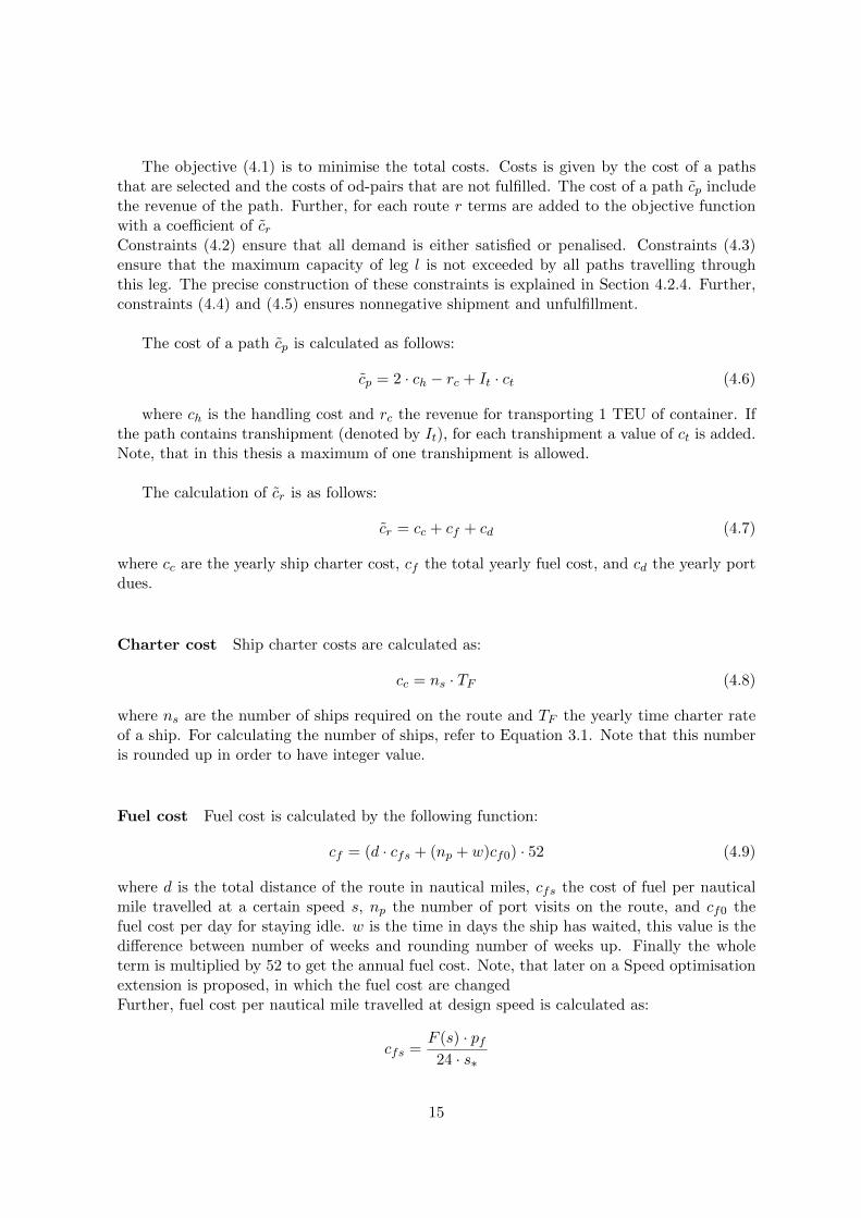
The objective (4.1) is to minimise the total costs. Costs is given by the cost of a pathsthat are selected and the costs of od-pairs that are not fulfilled. The cost of a path cp includethe revenue of the path. Further, for each route r terms are added to the objective functionwith a coefficient of crConstraints (4.2) ensure that all demand is either satisfied or penalised. Constraints (4.3)ensure that the maximum capacity of leg l is not exceeded by all paths travelling throughthis leg. The precise construction of these constraints is explained in Section 4.2.4. Further,constraints (4.4) and (4.5) ensures nonnegative shipment and unfulfillment.
The cost of a path cp is calculated as follows:
cp = 2 · ch − rc + It · ct (4.6)
where ch is the handling cost and rc the revenue for transporting 1 TEU of container. Ifthe path contains transhipment (denoted by It), for each transhipment a value of ct is added.Note, that in this thesis a maximum of one transhipment is allowed.
The calculation of cr is as follows:
cr = cc + cf + cd (4.7)
where cc are the yearly ship charter cost, cf the total yearly fuel cost, and cd the yearly portdues.
Charter cost Ship charter costs are calculated as:
cc = ns · TF (4.8)
where ns are the number of ships required on the route and TF the yearly time charter rateof a ship. For calculating the number of ships, refer to Equation 3.1. Note that this numberis rounded up in order to have integer value.
Fuel cost Fuel cost is calculated by the following function:
cf = (d · cfs + (np + w)cf0) · 52 (4.9)
where d is the total distance of the route in nautical miles, cfs the cost of fuel per nauticalmile travelled at a certain speed s, np the number of port visits on the route, and cf0 thefuel cost per day for staying idle. w is the time in days the ship has waited, this value is thedifference between number of weeks and rounding number of weeks up. Finally the wholeterm is multiplied by 52 to get the annual fuel cost. Note, that later on a Speed optimisationextension is proposed, in which the fuel cost are changedFurther, fuel cost per nautical mile travelled at design speed is calculated as:
cfs =F (s) · pf
24 · s∗
15

where F (s) the fuel consumption at speed s and pf the fuel price. Note, that F (s) is shownin Equation 3.2.
The cost per day for staying idle is calculated as:
cf0 = fF0 · pf
where fF0 the fuel consumption per day for staying idle.
Port dues The last term associated with route cost are the yearly dues paid to the port.This is calculated as:
cd = np · pd · 52 (4.10)
where np the number of ports visited on route and pd the price paid to enter the port. Thisamount is assumed to be the same for all ports. Eventually the whole term is multiplied by52 weeks in a year.
4.1.2 Extension 1: Multiple ships
In this section the PFM is extended with the option to choose between more than one shiptype for a route. The model gets more complex since each route r ∈ R is mapped to thenumber of ships in F. The properties of the model are as follows.Additional sets:
F : Fleet: contains all ship types s
Additional parameters:
crs : cost of route using ship type sqs : capacity of ship type s
Additional decision variables:
yrs : number of times route r, with allocated ship type s, is operated
The MIP problem is defined as
min∑p∈P
cpxp +∑
od∈OD
codLod +∑r∈R
crsyrs (4.11)
s.t. Lod +∑p3od
xp = dod ∀od ∈ OD (4.12)
∑jl∈p
xp ≤ Ql =∑s
qsyrs ∀l ∈ L (4.13)
xp, Lod ≥ 0 ∀p ∈ P,∀od ∈ OD (4.14)
yrs ∈ N (4.15)
Difference with the previous model is that the term cr is replaced by crs, which is theroute cost using a specific ship type.
16

4.1.3 Extension 2: Speed optimisation
Speed optimisation refers to adapting the speed of the travelling ship in order to reduce costs.Since, weekly service rate is used, the sailing speed can be adapted to arrive exactly on theend of a week. For this, the ship can either travel slower or faster to arrive exactly on theend of a week. For example, if at design speed the ship takes 2.5 weeks, it could go faster inorder to arrive in exactly 2 week, reducing the number of ships required on the route. Or, theship can travel slower which reduces the fuel cost used. The bunker consumption dependingon the speed change can be calculated using the function in Section 3.2. Using the speedoptimisation is done using the following algorithm:
Algorithm 1 Constraint construction
1: numberOfWeeks← ((((totalDistance/designSpeed) + numberOfPorts · 24)/24)/7)2: speedLow ← totalDistance/(168 · bnumberOfWeeksc − 24 · numberOfPorts)3: speedHigh ← totalDistance/(168 · dnumberOfWeekse − 24 · numberOfPorts)
4: costLowSpeed← calculateCostAtSpeed(Low)5: costHighSpeed← calculateCostAtSpeed(High)6: costDesignSpeed← calculateCostAtSpeed(Design)
7: optimalSpeedCost← min(costLowSpeed, costHighSpeed, costDesignSpeed)
4.2 Route generation
Main input of the model are the routes, and most of the variables in the model are createdbased on the routes. Therefore it is necessary to have a description of routes in the modelwhich can be processed further.Description of a route must be able to show the ports that are visited and the sequence inwhich they are visited. The following characteristics have been established to describe a route:
• Each port that is visited by a route is stated in the route.
• First port (beginning port) is equal to the last port (end port), since each route mustreturn to its starting point.
• The sequence explains in which order the ports are visited.
To simplify the information ports have been replaced by an unique integer number. InTable 4.1 the Id of each port is given.
The following, r1, is an example route (4.16), which starts at Belawan, travels to TanjungPriok, Tanjung Perak, Banjarmasin, and back to Belawan.
r1: {1, 2, 3, 4, 1} (4.16)
The generation of routes starts by permuting over al possibilities, in which a port is allowedonce in a route except for the beginning port. Although the model is capable of handlingmultiple visits of the same port in a route, due to high computation time for large number of
17

Id Port name
1 Belawan2 Tanjung Priok3 Tanjung Perak4 Banjarmasin5 Makasar6 Sorong
Table 4.1: Port name Ids
routes, this is limited to one port visit in a route. In Chapter 6, in the reference model fromWardana [2014], routes with multiple visits to the same ports are used. However in our ownsolution only routes with single port visits are used, since more routes are used in the model.
4.2.1 Path construction
Once the routes are generated, paths can be constructed. Basically, paths are described by anarray that looks like {o, d, r, i1, i2}, where o is origin, d the destination, r the route the pathbelongs to, i1 index of the paths origin in the route, and i2 index of the paths destination orthe route. In order to construct constraints it is required to know on which route the pathis operating. Subsequently, in order to determine which paths overlap with each other (makeuse of the same leg), in constraint construction, the indices are required. Index 1 (i1) showson which position the origin port of the path is located on the route r. And index 2 (i2) showson which position the destination port of the path is located on the same route. Therefore, apath contains a beginning port, a destination port, route number, and the indices of the twoports in the route. Based on the example (4.16) the following paths are constructed:
p1: {1, 2, 0, 0, 1} (4.17)
p2: {1, 3, 0, 0, 2} (4.18)
p3: {1, 4, 0, 0, 3} (4.19)
p4: {2, 1, 0, 1, 4} (4.20)
p5: {2, 3, 0, 1, 2} (4.21)
p6: {2, 4, 0, 1, 3} (4.22)
p7: {3, 1, 0, 2, 4} (4.23)
p8: {3, 2, 0, 2, 5} (4.24)
p9: {3, 4, 0, 2, 3} (4.25)
p10: {4, 1, 0, 3, 4} (4.26)
p11: {4, 2, 0, 3, 5} (4.27)
p12: {4, 3, 0, 3, 6} (4.28)
These descriptions of paths are interpreted differently than the description of routes. Apath description is summarised as:
1. Origin port ID
18

2. Destination port ID
3. Route ID
4. Index of origin port in route
5. index of destination port in route
Observe that routes are treated as circular routes, i.e. paths may be constructed withorigin-port within the route description and destination-port after the route description. Inmore detail, take example (4.28). Although at first glance to the route there seems to beno connection from port 4 to port 3, there actually is. Since routes are circular, the journeycontinuous after the end-port is reached. Therefore, for p12 a ship travels from 4 to 1, to 2,and eventually to 3.
4.2.2 Path construction with transhipment
The description of a path changes if this is a path with transhipment. Let the example (4.29)be another valid route in the model.
r2: {3, 5, 3} (4.29)
If transhipment is allowed, more paths are constructed with transhipment from one routeto another. As an example, when r1 and r2 are considered, the following is a path that isconstructed.
p13: {1, 3, 0, 0, 2}{3, 5, 1, 0, 1} (4.30)
In order to construct a path with transhipment, two routes are required. These routesmust have a port in common at which the transhipment can take place.Example (4.30) shows that a container travelling on a ship starting at port 1 along route r1is transhipped in port 3 to another ship travelling along route r2. The container eventuallyarrives at port 5. This is a path for the origin-destination pair 1-5, which was not availableat route r1.
4.2.3 Filtering
Both with the generation of routes and paths, the number of variables created grows rapidly.Therefore, some routes and paths are left out due to invalidity. And a filter is applied toroutes with regard to distance.
In route generation the following rules are used to filter:
• Validity: a certain order of port visits is not allowed more than once. E.g. route { 1, 2,3, 1 } is the same route as route { 2, 3, 1, 2 }.
• Filter: the total distance of a route must not exceed the maximal allowed distance.
For path construction the following rules are used:
19

• Validity: The origin-destination demand must exist. No paths are constructed for whichthere is no demand.
• Validity: Per route, only one path with the same origin-destination is allowed. In casethere are more than one, the shortest is chosen.
• Validity: The starting index (4th index in a path description) of a path must not belarger than the number of ports in the concerning route. This is in order to stop infinitecirculation.
4.2.4 Contraint construction
The constraints in (4.3) and (4.13) have the same algorithm with regard to selecting pathsthat overlap a certain leg (consecutive leg l). The following algorithms are used in the model.
Algorithm 2 Constraint construction
1: for all l in L do2: expression← empty3: for all p in P do4: if l.origin = p.origin AND l.destination = p.destination then5: expression← expression+ p6: goto next p
7: for all jl in p do8: if JumpLegOverlapsL(jl) then9: expression← expression+ p
10: goto next p
11: model← expression
Algorithm 2 explains the procedure to add constraints. For each consecutive leg l allpaths in P are checked whether it overlaps with this leg. The reason for iterating throughall legs in p (row 7) is due to paths with transhipment. Since these could have more than 1 leg.
Algorithm 3 is a procedure that returns true or false based on whether l and jl ∈ p overlap.This is the reason indices of origin and destination ports are recorded in the description ofa path. Namely every port in a route is numbered according to the sequence, i.e. beginningport has index 1, next port to be visited has index 2, etc. This is used in order to determinewhether paths travelling along a certain leg in route overlap with each other or not.Basically the algorithm checks certain properties and returns true if any of the statementsare hit, otherwise by default false is returned. Statement on row 2 checks whether both legsare on the same route. Statements on rows 3 and 4 simply check whether legs use the sameports. The remaining statements are explained by an example. Note that the first number inthe bracket represent the index of origin port and the second number the index of destinationport.
1. row 5: [1,4] [2,3] - jl falls between l
2. row 6: [2,3] [1,4] - jl starts before l and ends after l
20

Algorithm 3 Finding overlapping legs
1: procedure JumpLegOverlapsL(jl)2: if l.route 6= jl.route then return false
3: if l.originIndex = jl.destinationIndex then return true
4: if l.destinationIndex = jl.originIndex then return true
5: if l.originIndex < jl.originIndex AND l.destinationIndex > jl.originIndex thenreturn true
6: if jl.originIndex < l.originIndex AND jl.destinationIndex > jl.originIndex thenreturn true
7: if l.originIndex < jl.originIndex AND l.destinationIndex >jl.originIndex AND l.destinationIndex < jl.destinationIndex thenreturn true
8: Reverse statements and check again9: returnfalse
3. row 7: [1,3] [2,4] - jl starts between l and ends after l
Further the statements (row 5, 6, and 7) are checked again after reversing the statement.Since these situations can also occur and must be checked as well. Lastly if non of thestatements hit, the function returns false.
21

Chapter 5
Data
In this chapter the data available is evaluated according to the requirements defined in Section5.2. Due to incompleteness of data, modifications and simplifications are applied if necessary.This is summarised in Section 5.3.
5.1 Sources
There are two main sources from which data is acquired, these are data from Indonesia PortCorporation I-IV via Wardana [2014] and from Maersk shipping line via LINERLIB (Brouer[2015]). For location data, publicly available sources are used.
Data Wardana [2014] Via the Port Corporation I-IV data is available about, demandbetween ports (see Table 9.2), costs and revenues for the ports in Indonesia. Based on thisdata, in Wardana [2014] some assumptions and simplifications were made.
Data LINERLIB There is data available via Brouer [2015] about Maersk Shipping linewhich is used for the article published by Brouer et al. [2014]. In the following sections, thissource of information is denoted by LINERLIB. This source contains data about fleets (Table5.5) and, a subset of the ports (Table 9.3).
5.2 Requirements
In order to apply the Benchmark Liner Shipping model from Brouer et al. [2014], certain datais required. This is summarised Table 5.1.
22

Port list P Fleet list V Cargo demandlist C
Distance
Port αP Vessel class vF Origin port αC Origin port αD
Name nP Capacity cF Destination portβC
Destination portβD
Country oP TC rate TF Quantity qC Draft δP
Cabotage aP Draft δP Freight rate fC Distance dD
Region rP Min speed sFmin Max transit timetC
Latitude xP Max speed sFmax
Longitude yP Design speed vF∗Draft δP Fuel consumption
fF∗ , design speedMove cost mP Fuel consumption
fF0 , idletranshipment costtP
Quantity of ves-sels qF
Fixed port callcost fP
Variable port callcost vP
Table 5.1: Data requirements based on Benchmark Liner Shipping Brouer et al. [2014]
5.2.1 Port list
Ports A subset of 17 major ports in Indonesia are considered in Wardana [2014] through5 regions. For each region, a port called ”others” is created which is an aggregation of allthe remaining minor ports of that region. From LINERLIB there are 3 ports which coincidewith the ports used in Wardana [2014], these are Tanjung Priok (Jakarta), Tanjung Emas(Semarang), and Tanjung Perak (Surabaya).
Location The Langitude and Longitude of each of the 12 ports (excluding the ”others”)are gathered through publicly available sources (Ports.com [2014], [publisher]).
Draft size There were three sources of information about these data, namely throughWardana [2014], LINERLIB, and publicly available. This is summarised in Table 5.2.
23

Port name LINERLIB Wardana[2014]
Public
Tanjung Priok (Jakarta) 8 14Tanjung Emas (Semarang) 9.5 9Tanjung Perak (Surabaya) 9.5 12Belawan 10 15.2PekanbaruBatamPontianak 6 10Banjarmasin 7 9.1Makassar 12Bitung 12 23.2Ambon 10 23.2Sorong 20 23.2
Table 5.2: Draft data in meters according to various sources. Empty denotes there were nodata available.
Port costs The data about Move, Transhipment, Port call fixed, and Port call variablecosts is incomplete. This is due to that in LINERLIB only 3 of the 12 ports available, anddue to the fact that in Wardana [2014] cost were averaged and simplifications were made withregard to data. The cost parameters used by LINERLIB and in Wardana [2014] are presentedrespectively in Tables 5.4 and 5.3.
Port name Move cost Transhipmentcost
Port CallCost Fixed
Port CallCost PerFFE
Tanjung Priok (Jakarta) 135.00 62.00 2999.00 7.00Tanjung Emas (Semarang) 134.00 81.00 2926.00 10.00Tanjung Perak (Surabaya) 185.00 3.00 884.00 5.00
Table 5.3: Cost data in dollars based on LINERLIB
Revenue 215 Per TEU transportedShip Charter Cost 3,296,680 Per ship in a yearFuel Cost 78 Per nautical milePort Dues 628 Per port visitedHandling Cost 34 Per container handled
Table 5.4: Cost data in dollars based on Wardana [2014]
5.2.2 Fleets
The information about fleets is based on the data from Maersk through LINERLIB, which issummarised in Table 5.5.
24

Vessel class CapacityFFE
TCratedaily(fixedCost)
draft MinSpeed
MaxSpeed
DesignSpeed
Bunkerton perday atDesignSpeed
IdleCon-sump-tionton/day
Feeder 450 450 5000 8 10 14 12 18.8 2.4Feeder 800 800 8000 9.5 10 17 14 23.7 2.5Panamax 1200 1200 11000 12 12 19 18 52.5 4Panamax 2400 2400 21000 11 12 22 16 57.4 5.3Post panamax 4200 35000 13 12 23 16.5 82.2 7.4Super panamax 7500 55000 12.5 12 22 17 126.9 10
Table 5.5: Fleet data based on LINERLIB
5.2.3 Cargo demand
Quantity This data is gathered via Wardana [2014] and is summarised in Appendix Table9.1.
Freight rate The only available information about the freight rate can be found via War-dana [2014], namely a rate of $215 per TEU transported.
Max transit time Based on Wardana [2014], average time spent in port is 24 hours.Maximum distance between ports is 2879 nautical miles between Belawan and Ambon. Basedon an average speed of 18 knots per hour (Wardana [2014]), this implies a maximum traveltime of about one week.
5.2.4 Distance
Distance information is based on public data and is summarised in Appendix Table 9.2. Draftsize is decided based on the minimum between Origin port and Destination port. Suez traver-sal and Panama traversal is not applicable in this context, therefore these will be neglected.
5.3 Preprocessing
To be able to compare this model with a reference model, data and parameters are alignedin order to compare with the model from Wardana [2014].One of the tasks to compare is to use the same demand matrix. Wardana [2014] transformedthe original demand matrix (Appendix:Table 9.1) into a smaller set by aggregating the demandto a regional hub. The aggregation of ports into main ports is summarised in Table 5.6.
25

Main port Added ports
Belawan Pekanbaru, Batam, OthersTanjung PriokTanjung Perak Tanjung Emas, OthersBanjarmasin Pontianak, OthersMakasar Bitung, OthersSorong Ambon, Others
Table 5.6: Port aggregation. Source: Wardana [2014]
With others, the remaining ports in each of the 6 major regions is meant (see Ap-pendix:Table 9.1). Note that it is unclear from Wardana [2014] which ports are exactlymeant with ”others”. However, it is assumed this is done correctly.
5.3.1 Port aggregation
The aggregation of the ports into 6 main ports including the demand data is summarised inTable 5.7.
Belawan T. Priok T. Perak Banjarmasin Makasar Sorong Supply
Belawan - 348036 55016 4524 4212 1404 413192
T. Priok 350480 - 99632 212784 145496 24128 832520
T. Perak 53872 126724 - 19734 250640 113048 741624
Banjarmasin 4680 189124 181896 - 676 - 376376
Makassar 4732 182052 213668 3796 - - 404248
Sorong 2028 34372 113048 - - - 149448
Demand 415792 880308 663260 418444 401024 138580 2917408
Table 5.7: Yearly demand in TEU in case of port aggregation into 6 main ports. Source:Wardana [2014]
Both in supply and demand Belawan, T. Priok, and T. Perak have the most volume. It isexpected that these ports will be visited the most. Belawan and Sorong have little demandand supply also there distance is the largest among the ports. Thus, this origin-destinationpair is expected to have low or no volume.
5.4 Parameter setting / Assumptions
In this section, a summary is given with regard to which data is used from the various sourcesand what modifications/simplifications are applied. In the following sections, each subject isdiscussed separately. And the assumptions made for the PFM and Fleet Extension Modelare also discussed separately.
Fleet In order to compare the model with the reference, only one ship type is used as it isdone by Wardana [2014]. The characteristics of this ship is summarised in table 5.8. However,other ships are used as well, since there are ports in Indonesia that are capable of handling
26

each fleet. Therefore some of the fleets in the Table 5.5 are used. The exact fleet and itsresults are discussed in 6.2.3.
Vessel class CapacityFFE
TCratedaily(fixedCost)
draft MinSpeed
MaxSpeed
DesignSpeed
Bunkerton perday atDesignSpeed
IdleCon-sump-tionton/day
Panamax 1750 1750 15000 8 12 18 20 55 4.5
Table 5.8: Ship used by Wardana [2014]
Draft size The draft size is neglected in the model since only one type of ship is used,namely ship Panamax 1750 with a capacity of 3500 TEU. The ports are aggregated in sucha way that there is always a port within the region which able to handle this ship size.
Port costs In Wardana [2014] a move cost of $34 per container handled is used, while inthis model this is multiplied by two for loading and unloading. Port dues are $628 per portvisited and in line with Wardana [2014].
Fright rate In line with Wardana [2014] a freight rate of $215 is used per transportedcontainer.
Maximum transit time After experimenting with the model with regard to amount ofroutes versus computation time and route distance versus improvement, a maximum distanceof 4500 (16 days sailing) seems both practical for the model and a reasonable sailing time fora ship. This information is used during the route generation in order to filter out exceedingroutes.
5.5 Technique
The model is built using Java as a programming language with the use of IBM CPLEX12.6.0.0 solver and Java Combinatorics 2.1 Paukov [2000–2004] as external libraries. TheCPLEX solver is used in the model and the Combinatorics is used to generate routes bypermutation.A Mac operating system is used and the hardware consists of a processor of 2.5 GHz IntelCore i5 and a memory of 4 GB (1600 MHz DDR3).
27

Chapter 6
Results
In this Chapter the results are presented. First, the results from the reference model arediscussed in Section 6.1. Secondly, the results are discussed using route generation in Section6.2. In this section, all the extensions are discussed in separate. A base model is used tocompare each extension. There are three extensions, these are transhipment, Multiple Ships,and Speed Optimisation. The extensions are used separately, i.e. only 1 extension is enabledwhile others are disabled. Later, the extensions are combined together and this is called ALLsetting.
In advance, the fleet used in the following sections is summarised in 6.1. Note, that theId is used to describe what type of ship is used in the following sections. Further, ship type4 (Panamax 1750) is used whenever only 1 ship type is used. Since this is the only ship typeused in the Reference model by (Wardana [2014]).
Id Vessel classCapacityFFE
TC ratedaily
MinSpeed
MaxSpeed
DesignSpeed
Bunker ton/dayat designSpeed
Idle Cons.ton/day
1 Feeder 450 450 5000 10 14 12 18.8 2.42 Feeder 800 800 8000 10 17 14 23.7 2.53 Panamax 1200 1200 11000 12 19 18 52.5 44 Panamax 1750 1750 15000 12 20 18 55 4.55 Panamax 2400 2400 21000 12 22 16 57.4 5.3
Table 6.1: Fleet used
6.1 Reference model
In order to compare and verify the PFM model, the model from Wardana [2014] is used. Table6.2 summarises the results. Column Reference shows the result as reported by Wardana [2014].While Reference* is the result of the PFM using the same set of routes as in Reference. Thelast column, Reference*(ALL), contains the results using the same routes as in Referenceexcept that all settings/extensions are enabled. This is summarised in Table 6.4.
28

Reference Reference* Reference*(ALL)
# routes (input) 4 4 4# paths - 60 146# routes (output) 4 5 4# ships 11 13 10Weekly profit ($) 7,745,073 5,066,915 5,671,141Increase 100% 112%
Comp. time (sec) - 0.184 0.808
Cargo (TEU) 2,765,672 2,778,828 2,894,632Satisfied demand 0.95 0.95 0.99
Revenue ($) 594,619,480 597,448,020 622,345,880Trans. cost ($) 0 0 68,952Handling cost ($) 94,032,848 188,960,304 196,834,976Ship charter ($) 36,263,480 71,175,000 72,270,000Fuel cost ($) 60,762,936 72,853,444 57,456,224Port dues ($) 816,400 979,680 816,400Total costs ($) 191,875,664 333,968,428 327,446,552Profit ($) 402,743,816 263,479,592 294,899,328
Table 6.2: Results from Reference model(Wardana [2014]), the results of PFM using the sameroutes, and the results of PFM using same routes and all extensions and settings.
The first row, number of routes, shows the input size of the different models. The numberof paths are generated based on the input, which is discussed in Section 4.2.1. The numberof ships displays the amount of ships required for the solution. Weekly profit is calculatedbased on the Profit, which is based on a yearly basis. Computation time gives the amountof time it took to solve the model, the hardware specification are discussed in Section 5.5.Cargo shows the total amount of containers in TEU that are transported.Revenue is based on a freight rate of $215. transhipment cost is based on the amount tran-shipment multiplied by the handling cost of $34. Handling cost is calculated by multiplyingamount of Cargo with twice the handling cost cost (2 ·$34). Ship charter, Fuel cost, and Portdues are calculated based on the functions (4.8),(4.9), and (4.10) respectively.
6.1.1 Difference between PFM and Reference model
Although the Reference* setting of the PFM was meant to mirror the Reference model, thereare some differing interpretations with regard to cost calculations.The differences between thetwo models are summarised as:
• Transported cargo: Satisfied demand is larger in the Reference* solution than in theReference solution
• Handling cost: In Reference a handling cost of $34 is calculated once while in PFM thisvalue is calculated twice, once for loading and once for unloading.
29

• Fuel cost: In PFM idle consumption per day per port visit is also included in the Fuelcost, while this is neglected in Reference.
• Charter cost: In calculating the amount of ships required to satisfy weekly service, thetotal duration is calculated based on total travel time and port (stay) time. In theReference model the port time is ignored, while in PFM the port time is set to 24 hoursper visit.
6.1.2 Reference* solution
The following table summarises the solution to the PFM using the Reference* setting.
Route yrsDis-tance
Cargo(TEU)
# ofships
Shiptype
Shipcharter
Fuelcost
Portdues
Sp.
{1 2 3 4 3 2 1} 2 7,320 1,682,356 6 4 32,850,000 32,594,467 391,872 18{ 2 3 4 5 4 3 2} 2 4,476 728,676 4 4 21,900,000 20,256,167 391,872 18{ 2 3 5 6 4 3 2} 1 4,676 367,796 3 4 16,425,000 20,002,811 195,936 18
Total 5 16,472 2,778,828 13 71,175,000 72,853,444 979,680
Table 6.3: Solution: Reference* (PFM with the use of routes from Wardana [2014])
In the above table, Route displays the route based on the route description as discussedin Section 4.2. yrs is the variable in the model indicating the amount of times the routeis used (operated) per week. rs indicates a route r and a ship type s. Distance gives thetotal nautical miles travelled by a ship on the route. Number of ships displays the amount ofships required on the route to maintain weekly visits. Ship type shows the chosen ship thatoperates on the route. The id’s are given in Section 6.2.3. Id 4 is the Panamax 1750 whichis the same type as in Wardana [2014]. The Ship Charter, Fuel cost, and Port dues showthe cost in dollars for each route in separate. Finally, Speed shows the speed in knots per hour.
6.1.3 Reference*(ALL) solution
Using the same model from Reference* and enabling transhipment, Multiple Ships, and SpeedOptimisation has the following solution:
Route yrsDis-tance
Cargo(TEU)
# ofships
Shiptype
Shipcharter
Fuelcost
Portdues
Sp.
{ 1 2 3 4 5 3 2 1 } 1 4,205 1,211,132 3 5 22,995,000 13,155,683 228,592 12.51{ 1 2 3 4 5 3 2 1 } 1 4,205 1,211,132 3 5 22,995,000 13,155,683 228,592 12.51{ 2 3 4 5 4 3 2 } 1 2,238 503,672 2 5 15,330,000 11,788,774 195,936 16.00{ 2 3 5 6 4 3 2 } 1 4,676 499,200 3 5 22,995,000 15,364,047 195,936 12.99
Total 4 14,779 2,896,660 10 72,270,000 57,456,224 816,400
Table 6.4: Solution: PFM with the use of routes from Wardana [2014]) and enabling tran-shipment, Multiple Ships, and Speed Optimisation
Compared to the solution of Reference*, the solution of Reference*(ALL) has better re-sults. By using larger ships (ship type 5) more cargo can be transported. Although the Ship
30

Charter is more, due to the larger ships, making use of transhipment and Speed Optimisationresults in 1 less ship. Ship type 4 is sailing faster in order to preventing the need for an extraship (due to weekly service rates), and 2 out of 3 ships (ship type 5) sail slower in order toreduce fuel cost. Overall, with all the settings and extensions the solution improves with 12%.
The exact path flows for route { 1 2 3 4 5 3 2 1 } are given in the following table.
i r o d xpi cpi poi pdi index(poi ) index(pdi )
1 { 1 2 3 4 5 3 2 1 } 1 2 190372 -147 1 2 0 12 { 1 2 3 4 5 3 2 1 } 1 3 55016 -147 1 3 0 23 { 1 2 3 4 5 3 2 1 } 1 5 4212 -147 1 5 0 44 { 1 2 3 4 5 3 2 1 } 2 1 186316 -147 2 1 6 75 { 1 2 3 4 5 3 2 1 } 2 3 99632 -147 2 3 1 26 { 1 2 3 4 5 3 2 1 } 2 5 33072 -147 2 5 1 47 { 1 2 3 4 5 3 2 1 } 3 1 53872 -147 3 1 5 78 { 1 2 3 4 5 3 2 1 } 3 2 126724 -147 3 2 5 69 { 1 2 3 4 5 3 2 1 } 3 4 19864 -147 3 4 2 310 { 1 2 3 4 5 3 2 1 } 3 5 192452 -147 3 5 2 411 { 1 2 3 4 5 3 2 1 } 4 1 4680 -147 4 1 3 712 { 1 2 3 4 5 3 2 1 } 5 1 4732 -147 5 1 4 713 { 1 2 3 4 5 3 2 1 } 5 2 26520 -147 5 2 4 614 { 1 2 3 4 5 3 2 1 } 5 3 213668 -147 5 3 4 5
Table 6.5: Solution paths under Reference*(ALL) for route { 1 2 3 4 5 3 2 1 }.
Each row indicates a path and its characteristics are given in the columns. r denotes theroute the path pi belongs to. Note that, only the paths belonging to route { 1 2 3 4 5 3 2 1} are given in this table. Each path has an origin poi and a destination pdi , which must matcha demand origin o and a demand destination d. xpi denotes the amount of cargo transportedon path pi, which is used in the model as one variable. The cost belonging to the path pi isgiven by cpi .
Further, the indices of the origin and destination of paths with regard to route r are given.This is used in order to identify which paths are using the same leg. For example, for leg 1-2the first three paths, p1, p2, and p3 with the respective o-d’s 1-2, 1-3, and 1-5, have a totalcargo of 249,600 TEU. This is equal to the yearly capacity of ship type 5 (Panamax 2400).This means that the ship travelling from port 1 to 2, has a load/capacity ratio of 1. While forleg 2-3, which are used by paths: p5, p2, p3, and p6, a total of 191,932 TEU is transported.This results in a load ratio of 0.77.
6.2 Route generation
Here, the results from the model with the use of different settings are discussed. In all of thesettings same set of generated routes are used (a total of 72 routes). Routes are generated asdiscussed in Section 4.2 and are filtered based on a maximum distance of 4500 nautical miles.In the following subsection the solution of each setting is discussed separately.
31

BASE setting indicates the basic model without any modification to the PFM model. Undertranshipment the base model is modified to enable transhipment between routes. Multipleships is the first extension and opt. is the second extension as discussed in Sections 4.1.2 and4.1.3, respectively. Finally, the model is used using all settings together (ALL). The followingtable contains a summary of the different results.
BASE transhipmentMultipleships
Speedopt
ALL
# routes (input) 72 72 360 72 360# paths 500 16,976 500 500 16,976# routes (output) 8 7 7 8 7# ships 10 8 9 10 9Weekly profit ($) 5,757,357 5,799,822 5,783,703 6,124,640 6,304,356Increase 100% 101% 100% 106% 110%
Comp. time (sec) 1.264 83.987 5.512 0.958 7.267
Cargo (TEU) 2,904,980 2,764,372 2,890,363 2,904,980 2,917,408Satisfied demand 0.99 0.95 0.99 0.99 1.00
Revenue ($) 624,570,700 594,339,980 621,429,120 624,570,700 627,242,720Trans. cost ($) - 2,781,064 - - 3,334,448Handling cost ($) 197,538,640 187,977,296 196,545,024 197,538,640 198,383,744Ship charter ($) 54,750,000 43,800,000 58,035,000 54,750,000 53,655,000Fuel cost ( $) 72,213,736 57,570,392 65,508,719 53,082,375 43,422,556Port dues ( $) 685,776 620,464 587,808 718,432 620,464Total costs ($) 325,188,152 292,749,216 320,676,551 306,089,447 299,416,212Profit ($) 299,382,548 301,590,764 300,752,569 318,481,253 327,826,508
Table 6.6: Results under different settings
As it can be observed from the above table, each setting/extension results in a betterresult. However, the speed optimisation extension is by far the best extension contributingto improve the model. Although it uses more routes and more ships it manages to have moreprofit by increasing the cargo shipped and reducing its total fuel cost.Enabling transhipment does not improve the BASE solution much, in the solution less shipsare used in and less cargo is transported in order to reduce costs.Further, note that the computation time in the transhipment setting is much more than theALL setting even though there are the same amount of variables. We expected to have alarger computation time, however CPLEX managed to solve it quicker.Multiple ship extension does not improve much, this could be due to the fact that the demandis already largely satisfied in the BASE solution. The amount of cargo transported is less,however the costs are less with regard to fuel costs and port dues.It is noteworthy that when using all settings/extensions together (ALL) the increase (10%)in profit is better than the sum of the three individual improvements.In the following sections, the solution of each setting/extension is discussed in separate.
32

6.2.1 BASE solution
This is the basic setting in which the model is kept as simple as possible. That is no extensionsor extra settings are enabled and is meant to be a base result to compare the other settingsand extensions.The following table displays the characteristics of the BASE solution.
Route yrsDis-tance
Cargo(TEU)
# ofships
Shiptype
Shipcharter
Fuelcost
Portdues
Sp.
{ 1, 2, 1 } 2 4,256 667,160 2 4 10,950,000 17,488,178 130,624 18{ 2, 4, 3, 2 } 1 1,380 396,240 1 4 5,475,000 6,015,967 97,968 18{ 1, 2, 3, 4, 1 } 1 3,260 429,208 2 4 10,950,000 13,855,544 130,624 18{ 2, 5, 2 } 1 1,612 327,496 1 4 5,475,000 6,862,122 65,312 18{ 3, 5, 3 } 1 1,040 364,000 1 4 5,475,000 4,775,911 65,312 18{ 3, 5, 4, 3 } 1 1,201 367,120 1 4 5,475,000 5,363,114 97,968 18{ 2, 6, 3, 2 } 1 4,356 353,756 2 4 10,950,000 17,852,900 97,968 18
Total 8 17,105 2,904,980 10 54,750,000 72,213,736 685,776
Table 6.7: Solution: Base model
In comparison to the Reference* solution (Table 6.4) the routes selected have less shipsand less travel distance. This enables to reduce fuel and ship charter costs while increasing theamount of cargo transported. Overall the BASE solution compared to Reference*, increasedthe profit by 13%.
6.2.2 Transhipment solution
As described in Section 4.2.2 the model is set to allow transhipment. This does not changethe PFM, however the amount of variables increase vastly. This explains the extreme increasein the computation time. The solution of this setting is summarised in the following table.
Route yrsCargo(TEU)
Cargo(TEU)
# ofships
Shiptype
Shipcharter
Fuelcost
Portdues
Sp.
{ 1, 2, 1 } 2 4,256 728000 2 4 10,950,000 17,488,178 130,624 18{ 2, 3, 4, 2 } 1 1,380 479,596 1 4 5,475,000 6,015,966 97,968 18{ 2, 4, 3, 2 } 1 1,380 538,876 1 4 5,475,000 6,015,966 97,968 18{ 1, 2, 4, 3, 1 } 1 3,494 417,456 2 4 10,950,000 14,708,994 130,624 18{ 2, 5, 2 } 1 1,612 364,000 1 4 5,475,000 6,862,122 65,312 18{ 3, 5, 4, 3 } 1 1,201 371,020 1 4 5,475,000 5,363,114 97,968 18{ 3, 4, 6, 5, 3 } 1 3,800 364,676 2 4 10,950,000 15,825,044 130,624 18
Total 7 13,629 2,846,168 8 43,800,000 57,570,392 620,464
Table 6.8: Solution: Transhipment
Compared to the BASE solution (Table 6.7) this solutions requires 1 less route and 1 lessship. Less cargo is transported in order to reduce costs with regard to using ships. Thisis possible due to the ability to transport cargo through transhipment, which compensatesfor the smaller fleet size. Note that the total cargo transported in Table 6.8 is higher thanin Table 6.6, due to double counting. In Table 6.8 shows the cargo transported per route
33

independently of other routes.The following table describes the transhipments between the routes.
i r1 r2 o d xpi cpipoi1in r1
pdi1in r1
poi2in r2
poi2in r2
1 { 1, 2, 1 } { 2, 3, 4, 2 } 1 3 15,964 -113 1 2 2 32 { 2, 5, 2 } { 3, 5, 4, 3 } 2 4 17,680 -113 2 5 5 43 { 2, 4, 3, 2 } { 1, 2, 1 } 3 1 13,520 -113 3 2 2 11 { 2, 4, 3, 2 } { 2, 5, 2 } 3 5 18,824 -113 3 2 2 52 { 3, 4, 6, 5, 3 } { 2, 4, 3, 2 } 6 2 15,808 -113 6 3 3 2
Table 6.9: Solution paths under the setting Transhipment
The table only shows the transshipment paths (i.e. paths with two jump legs) that arein the optimal solution. While, the model also contains normal paths which only have oneleg in it. In the model each transhipment path is treated as a normal path, meaning it isrepresented by only one variable xp with its own cost cp. Each path pi, in the table, consistsof two jump legs: pi1 and pi2 . Further, each leg contains an origin and a destination belongingto a route. Note, that the routes of legs in a transhipment path cannot be on the same route.And, that some properties are left out of the table, such as origin and destination of paths,i.e. respectively po and pd, which are the same as o and d.In comparison to normal paths, as in Table 6.5, the cost are less negative. This is due to anextra handling cost of $34.
6.2.3 Extension 1: Multiple ships solution
The model is extended as described in Section 4.1.2 in which there are 5 ship types. All ofthe ships described in Table 6.1 are used. The solutions are described in the following table.
Route yrsDis-tance
Cargo(TEU)
# ofships
Shiptype
Shipcharter
Fuelcost
Portdues
Sp.
{ 1, 2, 1 } 1 2,128 364,000 1 4 5,475,000 8,744,089 65,312 18{ 3, 4, 3 } 1 656 306,696 1 4 5,475,000 3,375,378 65,312 18{ 2, 4, 3, 2 } 1 1,380 545,428 1 5 7,665,000 6,999,233 97,968 16{ 1, 2, 3, 4, 1 } 1 3,260 519,480 2 5 15,330,000 16,115,028 130,624 16{ 2, 5, 2 } 1 1,612 327,496 1 4 5,475,000 6,862,122 65,312 18{ 3, 5, 3 } 1 1,040 463,268 1 5 7,665,000 5,559,970 65,312 16{ 2, 3, 6, 2 } 1 4,356 364,000 2 4 10,950,000 17,852,900 97,968 18
Total 7 14,432 2,890,368 9 58,035,000 65,508,719 587,808
Table 6.10: Solution: Multiple ships
Compared to the BASE solution the routes that entered the solution are: E1:{ 3, 4, 3 }and E2:{ 2, 3, 6, 2 }, while routes that left the solution are: L1:{ 3, 5, 4, 3 } and L2:{ 2,6, 3, 2 }. It appears that E1 is switched with L1 and E2 with L2. Since more cargo can betransported, by using a larger ship (5), on E2 instead of L2, visit to port 2 in L1 becomesunnecessary.
34

6.2.4 Extension 2: Speed optimisation solution
The model is extended as discussed in Section 4.1.3. The impact of this extension is larger,since the evaluation of routes become different. That is, routes that were too expensive tooperate become more profitable.
Route yrsDis-tance
Cargo(TEU)
# ofships
Shiptype
Shipcharter
Fuelcost
Portdues
Sp.
{ 1, 2, 1 } 2 4,256 689,676 2 4 10,950,000 16,970,176 130,624 17.73{ 2, 4, 3, 2 } 1 1,380 380,224 1 4 5,475,000 3,917,296 97,968 14.38{ 1, 2, 3, 4, 1 } 1 3,260 421,356 2 4 10,950,000 7,935,867 130,624 13.58{ 2, 5, 2 } 1 1,612 327,496 1 4 5,475,000 3,847,127 65,312 13.43{ 3, 4, 5, 3 } 1 1,201 364,676 1 4 5,475,000 2,725,691 97,968 12.51{ 3, 5, 4, 3 } 1 1,201 367,796 1 4 5,475,000 2,725,691 97,968 12.51{ 2, 6, 3, 2 } 1 4,356 359,456 2 4 10,950,000 14,960,526 97,968 16.50
Total 8 17,266 2,904,980 10 54,750,000 53,082,375 718,432
Table 6.11: Solution: Speed optimisation
From the BASE solution only three routes are left in the solution, namely { 1, 2, 1 }, {2,4, 3, 1 }, and { 2, 5, 2 }. These routes have lower cost in this extension than in the BASEsolution, due to more optimal use ships speed. The reason for this considerable change inthe selection of routes is due to the fact that routes have become less expensive. Further, allthe ships sail slower in order to reduce the fuel cost, this compensates for the extra ships. Intotal there is an extra route and an extra ship available.
6.2.5 All settings combined solution
In ALL, the previously mentioned settings and extensions are enabled. That is, transhipmentis allowed, the allocation of ships to routes can be chosen from multiple ships, and speedoptimisation is enabled to drive slower or faster in order to reduce costs. The resultingsolution is shown in the following table.
Route yrsDis-tance
Cargo(TEU)
# ofships
Shiptype
Shipcharter
Fuelcost
Portdues
Sp.
{ 1, 2, 1 } 1 2,128 496,600 1 5 7,665,000 12,521,954 65,312 17.73{ 2, 3, 4, 2 } 1 1,380 479,804 1 4 5,475,000 3,917,296 97,968 14.38{ 2, 4, 3, 2 } 1 1,380 490,100 1 4 5,475,000 3,917,296 97,968 14.38{ 1, 2, 3, 4, 1 } 1 3,260 368,888 2 4 11,000,000 7,935,867 130,624 13.58{ 2, 5, 2 } 1 1,612 358,852 1 4 5,475,000 3,847,127 65,312 13.43{ 3, 5, 4, 3 } 1 1,201 533,208 1 5 7,665,000 3,920,459 97,968 12.51{ 3, 6, 3 } 1 3,632 288,028 2 4 11,000,000 7,362,558 65,312 12.61
Total 7 14,593 3,015,480 9 53,755,000 43,422,556 620,464
Table 6.12: Solution: Using Transhipment, Multiple ships and Speed optimisation
Since, Speed optimisation solution has the best profit, the ALL solution is compared tothis. The differences are caused by transhipment possibilities and changing ships. Based on
35
the Speed optimisation solution only three routes have left the solution, namely: { 1, 5, 2,1 }, { 3, 4, 5, 3 }, and { 2, 3, 6, 2 }. While, only { 2, 3, 4, 2 } and { 3, 6, 3 } entered thesolution. In total, ALL solution requires 1 route and 2 ships less to satisfy more demand thanSpeed optimisation solution, namely all of the demand.
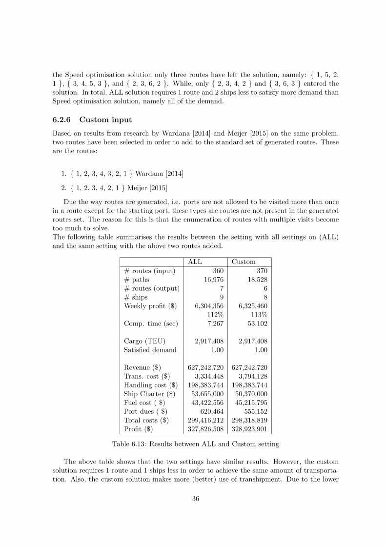
6.2.6 Custom input
Based on results from research by Wardana [2014] and Meijer [2015] on the same problem,two routes have been selected in order to add to the standard set of generated routes. Theseare the routes:
1. { 1, 2, 3, 4, 3, 2, 1 } Wardana [2014]
2. { 1, 2, 3, 4, 2, 1 } Meijer [2015]
Due the way routes are generated, i.e. ports are not allowed to be visited more than oncein a route except for the starting port, these types are routes are not present in the generatedroutes set. The reason for this is that the enumeration of routes with multiple visits becometoo much to solve.The following table summarises the results between the setting with all settings on (ALL)and the same setting with the above two routes added.
ALL Custom
# routes (input) 360 370# paths 16,976 18,528# routes (output) 7 6# ships 9 8Weekly profit ($) 6,304,356 6,325,460
112% 113%Comp. time (sec) 7.267 53.102
Cargo (TEU) 2,917,408 2,917,408Satisfied demand 1.00 1.00
Revenue ($) 627,242,720 627,242,720Trans. cost ($) 3,334,448 3,794,128Handling cost ($) 198,383,744 198,383,744Ship Charter ($) 53,655,000 50,370,000Fuel cost ( $) 43,422,556 45,215,795Port dues ( $) 620,464 555,152Total costs ($) 299,416,212 298,318,819Profit ($) 327,826,508 328,923,901
Table 6.13: Results between ALL and Custom setting
The above table shows that the two settings have similar results. However, the customsolution requires 1 route and 1 ships less in order to achieve the same amount of transporta-tion. Also, the custom solution makes more (better) use of transhipment. Due to the lower
36

amount of ships in the custom solution, the ships travel more. Therefore the fuel cost arehigher at Custom. However, due to having one less ship in custom solution, the ship chartercosts and port dues compensate for more travelling. This results in a higher profit.The solution of the custom setting is described in the following table.
Route yrsDis-tance
Cargo(TEU)
# ofships
Shiptype
Shipcharter
Fuelcost
Portdues
Sp.
{ 1, 2, 1 } 1 2,128 329,784 1 4 5,475,000 8,485,088 65,312 17.73{ 2, 4, 3, 2 } 1 1,380 501,696 1 4 5,475,000 3,917,296 97,968 14.38{ 2, 5, 2 } 1 1,612 360,776 1 4 5,475,000 3,847,127 65,312 13.43{ 3, 5, 4, 3 } 1 1,201 535,132 1 5 7,665,000 3,920,459 97,968 12.51{ 3, 6, 3 } 1 3,632 288,028 2 4 11,000,000 7,362,558 65,312 12.61{ 1, 2, 3, 4, 2, 1 } 1 3,508 1,013,584 2 5 15,300,000 17,683,267 163,280 16.24
Total 6 13461 3,029,000 8 50,390,000 45,215,795 555,152
Table 6.14: Solution: Using ALL settings and two custom routes
In comparison to the solution of ALL setting (Table 6.12), routes { 2, 3, 4, 2 } and { 1,2, 3, 4, 1 } have been replaced by the new introduced custom route { 1, 2, 3, 4, 2, 1 }. Abigger ship is used on the custom route and the amount of cargo transported on the customroute is more than the two replaced routes combined. Also, note that the first introducedcustom route has not been used. Therefore, there is not enough evidence to conclude thatthese types of routes (multiple visits) always have better results.
6.3 Conclusion
A reference model is obtained from Wardana [2014] and a Reference* setting is created, whichis the PFM model based on the same parameters, however with different (more stringent) costcalculations. This model, due to difference in cost calculation, performed worse as expected.However, using the same cost calculation as in Reference, Reference* performs better.Then a BASE solution is solved, based on a set of 72 routes, which are generated by enumer-ating through six ports and filtering based on a maximum distance of 4500 mi.This model is then extended with enabling transhipment. This did not improve BASE solu-tion as much as expected, however this is due to having little room for improvement. Sincethe BASE solution already satisfied considerable amount of demand.Multiple ship extension improved the BASE solution only slightly. The improvement is dueto being able to transport more on a larger ship.Speed optimisation improved the BASE solution the most, and also has a more different so-lution then Transhipment setting and Multiple ship extension. The reason for this is due tochange in route costs. Routes that were too expensive have become less expensive.In the ALL solution, all settings and extensions are enabled. As expected, the combinationof the different extension improved the solution.Finally, in Section 6.2.6, based on the contextual situation, two custom routes are addedto the set of routes. This resulted in choosing one of the two added routes in the optimalsolution, improving the total profit.
37

Chapter 7
Conclusion
The thesis is conducted to improve the liner-shipping network in Indonesia. The goal was todetermine the best liner shipping network for Indonesian ports using a mathematical model.In order to obtain this, first an appropriate model is found through a literature review. Themodel used in this thesis is the Path Formulation Model (PFM) based on Mulder [2015] (Sec-tion 4.1.1). This model is then extended such that it is able to choose which ship to use ona route (Section 4.1.2) from a set of ships and altering the speed in order to reduce costsassociated with a route. The last extension meant sailing slower in order to reduce fuel costor sailing faster in order to meet weekly service times.
Next to finding a mathematical model, a method has been implemented to generate routes,which serve as input for the PFM. The routes were generated based on six hub ports. Thesix ports were enumerated through all possibilities, and then filtered based on similarity anddistance.
Next, in Chapter 5 the context of Indonesian ports have been investigated and the model isadapted to fit the situation. That means, creating hub-ports to decrease the amount of portsand aggregating demand. Further simplifications/assumptions were made with regard to shipsize, costs, and fleets due to inconsistency in data.
In Chapter 6 the results have been discussed. This includes results from the reference solutionas well as the different settings and extensions. The Reference solution had some less strin-gent cost calculations, which were different from the PFM model. This caused discrepancybetween the PFM and Reference solution. However, the Reference model did help to verifythe PFM model.
The results from the different settings were compared to a BASE solution. Each exten-sion/setting improved the BASE solution. Namely, enabling transhipment in the model im-proved the profit with 1%, extending the model to choose from multiple ships did not improvemuch, and extending the model with speed optimisation improved it by 6%. In the ALL set-ting, with all the three settings/extensions enabled, resulted in an improvement of 12% withregard to the BASE solution and 24% with regard to the Reference* solution. This resultedin a weekly profit of $ 6,304,356 using the following routes: { Belawan, T. Priok, Belawan },{ T. Priok, T. Perak, Banjarmasin, T. Priok }, { T. Priok, Banjarmasin, T. Perak, T. Priok
38

}, { Belawan, T. Priok, T. Perak, Banjarmasin, Belawan }, { T. Priok, Makassar, T. Priok}, { T. Perak, Makassar, Banjarmasin, T. Perak }, and { T. Perak, Sorong, T. Perak }.
39

Chapter 8
Discussion
Although the model has reasonable performance, both in speed and in the optimal solution,there are still some limitations to the model. In the Section 6.2.6 custom routes are addedwhich are of a different type of than the generated routes in this thesis. Namely, the generatedroutes have single port visit, while the custom route is a pendulum route with multiple visitsto the same route. One of the two custom routes is also selected in the optimal solution.Therefore, pendulum routes might have a better solution. However, enumeration of pendu-lum routes results in too many routes to solve.
Further, due to incompleteness of data many simplifications were made about the data. There-fore, a more realistic solution could be obtained once the data becomes more complete. Forinstance the cost for all paths are assumed the same. This could be differentiated based ondistance. Further, a differentiation could be made based on ports. Namely, all ports areassumed to have same port dues and handling cost. The computation time is not expectedto increase much due to these kind of changes.
Although in the ALL solution all of the demand was satisfied, this does not necessarily haveto be the case. Due profit maximisation some ports could be ignored due to high costs. Inorder to improve overall profitability and economic growth of the region, the balance can bealtered using government funding and sanctioning. This could be accomplished in the modelby increasing or lowering the lost sales cost (cod) assigned to unsatisfied demand (Lod).
40

Bibliography
R. Agarwal and Ergun. Ship scheduling and network design for cargo routing in liner shipping.Transportation Science, 42(2):175–1968, 2008.
Patrick M Alderton. Reeds Sea Transport: Operation and Economics. Bloomsbury Publishing,2010.
J. F. Alvarez. Joint routing and deployment of a fleet of container vessels. Maritime Econom.Logist., 11(2):186–208.
M. Bell, Liu X, Angeloudis P, Fonzone A, and Hosseinloo SH. A frequency-based maritimecontainer assignment model. Transportation Res. Part B, 45(8):1152–1161, 2011.
L. C. Blancas and M. Baher El-Hifnawi. Facilitating Trade Through Competitive, Low-carbonTransport: The Case for Vietnam’s Inland and Coastal Waterways. World Bank Publica-tions, 2013.
T.B. Boffey, E.D. Edmond, A.I. Hinxman, and C.J. Pursglove. Two approaches to schedulingcontainer ships with an application to the north atlantic route. J. Oper. Res. Soc., 30(5):413–425, 1979.
A. Branch and M. Stopford. Maritime economics. Routledge, 2013.
B. Brouer. Linerlib. https://github.com/blof/LINERLIB, 2015. 2015-08-10.
B. Brouer, D. Pisinger, and S. Spoorendonk. Liner shipping cargo allocation with repositioningof empty containers. INFOR, 49(2):109–124, 2011.
B. Brouer, J. F. Alvarez, and C. E. M. Plum. A base integer programming model andbenchmark suite for liner-shipping network design. Transportation Science, 48(2):281–312,2014.
T. N. Chuang, C. T. Lin, J. Y. Kung, and L. M. Lin. Planning the route of container ships:A fuzzy genetic approach. Expert Systems Appl., 37(4):2948–2956, 2010.
K. Fagerholt. Optimal fleet design in a ship routing problem. Internat. Transactions Oper.Res., 6(5):453–464, 1999.
K. Fagerholt. Designing optimal routes in a liner shipping problem. Maritime Policy andManagement, 31(4):259–268, 2004.
A. Imai, K. Shintani, and S. Papadimitriou. Multi-port vs. hub-and- spoke port calls bycontainerships. Transportation Res. Part E, 45(5):740–757, 2009.
41

D. E. Lane, T. D. Heaver, and D. Uyeno. Planning and scheduling for efficiency in linershipping. Maritime Policy Management, 14(2):109–125, 1987.
S. A. Lawrence. International sea transport: The years ahead. 1972.
J. Meijer. Creating a liner shipping network design. BSc thesis, Erasmus University Rotter-dam, 2015.
Q. Meng and T. Wang. A scenario-based dynamic programming model for multi-period linership fleet planning. Transportation Res. Part E, 47(4):401?413, 2011.
Q. Meng, S. Wang, H. Andersson, and K. Thun. Containership routing and scheduling in linershipping: Overview and future research directions. Transportation Science, 48(2):265–280,2014.
J. Mulder. Will liner ships make fewer port calls? Working paper, 2015.
J. Mulder and R. Dekker. Methods for strategic liner shipping network design. EuropeanJournal of Operational Research, 2013.
Dmytro Paukov. GNU java combinatorics library 2.1.http://github.com/dpaukov/combinatoricslib, 2000–2004.
R. Pesenti. Hierarchical resource planning for shipping com- panies. Eur. J. Oper. Res., 86(1):91–102, 1995.
Ports.com. World seaports catalogue, marine and seaports marketplace, November 2014.URL http://ports.com/.
Mark E. Waters (publisher). Wps, November 2014. URLhttp://www.worldportsource.com/.
K. Rana and R. G. Vickson. A model and solution algorithm for optimal routing of a time-chartered containership. Transportation Sci., 22(2):83–95, 1988.
L. B. Reinhardt and D. Pisinger. A branch and cut algorithm for the container shippingnetwork design problem. Flexible Services Manufacturing J., 24(3):349–374, 2012.
E. Sambracos, J. A. Paravantis, C.D. Tarantilis, and C.T. Kiranoudis. Dispatching of smallcontainers via coastal freight liners: The case of the aegean sea. Eur. J. Oper. Res., 152(2):365–381, 2004.
K. Shintani, A. Imai, E. Nishimura, and S. Papadimitriou. The con- tainer shipping networkdesign problem with empty container repositioning. Transportation Res. Part E, 43(1):39–59, 2007.
D. P. Song and J. X. Dong. Cargo routing and empty container repo- sitioning in multipleshipping service routes. Transportation Res. Part B, 46(10):1556–1575, 2012.
S. Veldman, C. Glansdorp, and R. Kok. Economies of size of large containerships based oninternal and external costs. International Journal of Decision Sciences, Risk and Manage-ment, 3(3-4):384–400, 2011.
42

S. Wang and Q. Meng. Liner ship fleet deployment with container transshipment operations.Transportation Res. Part E, 48(10):470–484, 2012.
W. Wardana. Centre gravity model and network design to determine route of liner shipping:The case of east-west container shipping corridor in indonesia. 2014.
43

Chapter 9
Appendix
44

BLW
PK
BB
TM
OT
PR
TP
ET
EM
OP
TK
BJM
OM
KS
BT
GO
AM
BS
RG
OT
ota
lB
LW
4135
1030
2357
5245
PK
B73
8738
BT
M66
128
6424
27
804
O115
91159
TP
R42
63681
774
102
212
7564
112
2116
9011
81
2487
243
667
353
44
15948
TP
E98
947
1532
515
9921
91
1773
114
61901
472
292
1410
13357
TE
M0
O905
905
PT
K133
07
5934
281458
BJM
1674
121
815
9921
13
2941
O108
918
922981
MK
S57
34
2638
1279
3719
54240
BT
G85
992
923
13155
1979
O4
1901
1905
AM
B67
462
529
SR
G39
255
281
575
O339
1431
1770
Tot
al
5325
681
968
102
2169
2912
114
064
113
0734
4833
72453
0162
51907
539
672
1454
Tab
le9.1
:D
emand
data
inT
EU
(War
dan
a[2
014
])S
um
atra
:B
elaw
anB
LW
,P
ekan
bar
uP
KB
,B
ata
mB
TM
,O
ther
sO
Jav
a:T
an
jun
gP
riok
TP
R,T
anju
ng
Per
ak
TP
E,
Tan
jun
gE
mas
TE
M,
OK
alim
anta
n:
Pon
tian
akP
TK
,B
an
jarm
asi
nB
JM
,O
Su
law
esi:
Maka
ssar
MK
S,
Bit
un
gB
TG
,O
Res
tof
Ind
ones
ia:
Am
bon
AM
B,
Sor
ong
SR
G,
O
45
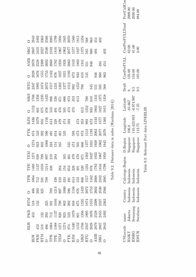
BLW
PK
BB
TM
OT
PR
TP
ET
EM
OP
TK
BJM
OM
KS
BT
GO
AM
BS
RG
OB
LW
453
518
486
1064
148
812
7112
7487
414
3011
5217
0823
472028
2879
2807
2843
PK
B45
3132
293
712
113
792
092
352
310
7980
1135
619
951676
2528
2455
2492
BT
M518
132
325
591
101
679
980
239
295
867
5123
518
741555
2399
2327
2363
O48
6293
325
789
121
499
710
0059
611
5687
614
33207
21753
2602
2530
2566
TP
R10
64712
591
789
438
210
324
491
614
553
806
151
71162
2068
2102
2085
TP
E14
88113
7101
6121
443
828
415
465
432
849
1520
1231
876
1782
1816
1799
TE
M12
71920
799
997
210
284
165
461
479
470
671
138
21027
1933
1967
1950
O12
74923
802
1000
324
154
165
535
474
505
666
137
71021
1928
1962
1945
PT
K87
4523
392
596
491
654
461
535
593
473
873
1512
1193
2063
2077
2070
BJM
1430
107
995
8115
6614
328
479
474
593
473
353
992
673
1543
1577
1560
O11
52801
675
876
553
491
470
505
473
473
613
125
2933
1803
1827
1815
MK
S170
813
56123
5143
380
652
067
166
687
335
361
3790
610
1341
1375
1358
BT
G234
719
95187
4207
215
17123
113
8213
7715
1299
212
5279
0545
551
585
568
O20
28167
6155
5175
311
62876
1027
1021
1193
673
933
610
545
946
980
963
AM
B287
925
28239
9260
220
68178
219
3319
2820
6315
4318
03134
155
1946
494
454
SR
G28
07245
5232
7253
021
02181
619
6719
6220
7715
7718
2713
75585
980
494
402
O28
43249
2236
3256
620
85179
919
5019
4520
7015
6018
1513
58568
963
454
402
Tab
le9.2
:D
ista
nce
dat
ain
mil
es(W
ard
ana
[2014
])
UN
Loco
de
nam
eC
ou
ntr
yC
abota
ge
Reg
ion
DR
egio
nL
ongi
tud
eL
atit
ud
eD
raft
Cost
Per
FU
LL
Cost
Per
FU
LLT
rnsf
Port
Call
Cost
Fix
edP
ort
Call
Cost
Per
FF
EID
JK
TJaka
rta
Ind
ones
iaIn
don
esia
Sin
gap
ore
106.
8-6
1.667
8135.0
062.0
02999.0
07.0
0ID
SR
GS
emar
an
gIn
don
esia
Ind
ones
iaS
inga
por
e11
0.42
3.95
3-6
.974
.997
9.5
134.0
081.0
02926.0
010.0
0ID
SU
BS
ura
bay
aIn
don
esia
Ind
on
esia
Sin
gap
ore
112.
75-7
.25
9.5
185.0
03.0
0884.0
05.0
0
Tab
le9.
3:R
elev
ant
Por
td
ata
LIN
ER
LIB
46