Content-Based Social Recommendation withPoisson Matrix Factorization

Eliezer de Souza da Silva1, Helge Langseth1, and Heri Ramampiaro1

Norwegian University of Science and Technology (NTNU)Department of Computer Science

NO-7491 Trondheim, Norway{eliezer.souza.silva, helge.langseth, heri}@ntnu.no

Abstract. We introduce Poisson Matrix Factorization with Contentand Social trust information (PoissonMF-CS), a latent variable prob-abilistic model for recommender systems with the objective of jointlymodeling social trust, item content and user’s preference using Poissonmatrix factorization framework. This probabilistic model is equivalent tocollectively factorizing a non-negative user–item interaction matrix anda non-negative item–content matrix. The user–item matrix consists ofsparse implicit (or explicit) interactions counts between user and item,and the item–content matrix consists of words or tags counts per item.The model imposes additional constraints given by the social ties be-tween users, and the homophily effect on social networks – the tendencyof people with similar preferences to be socially connected. Using thismodel we can account for and fine-tune the weight of content-basedand social-based factors in the user preference. We develop approxi-mate variational inference algorithm and perform experiments compar-ing PoissonMF-CS with competing models. The experimental evaluationindicates that PoissonMF-CS achieves superior predictive performanceon held-out data for the top-M recommendations task. Also, we observethat PoissonMF-CS generates compact latent representations when com-pared with alternative models while maintaining superior predictive per-formance.

Keywords: Probabilistic Matrix Factorization, Non-negative Matrix Fac-torization, Hybrid Recommender Systems, Poisson matrix factorization

1 Introduction

Recommender systems have proven to be a valuable component in many applica-tions of personalization and Internet economy. Traditional recommender systemstry to estimate a score function mapping each pair of user and item to a scalarvalue using the information of previous items already rated or interacted by theuser [1]. Recent methods have been successful in integrating side information ascontent of the item, user context, social network, item topics, etc. For this pur-pose a variety of features should be taken into consideration, such as the routine,the geolocation, spatial correlation of certain preferences, mood and sentiment

analysis, as well as social relationships such as “friendship” to others users or“belonging” to a community in a social network [2]. In particular, a rich area ofresearch has explored the integration of topic models and collaborative filteringapproaches using principled probabilistic models [3–5]. Another group of modelshas been developed to integrate social network information into recommendersystems using user–item ratings with extra dependencies [6] or constraining andregularizing directly the user latent factors with social features [7, 8]. Finally,some models have focused on the collective learning of both social features andcontent features, constructing hybrid recommender systems [5, 9, 10].

Our contribution is situated within all these three groups of efforts: we pro-pose a probabilistic model that generalizes both previous models by jointly mod-eling content and social factors in the preference model applying Poisson-Gammalatent variable models to model the non-negativeness of the user–item ratingsand induce sparse non-negative latent representation. Using this joint model wecan generate recommendations based on the estimated score of non-observeditems. In this article, we formulate the problem (Section 1.1), describe the pro-posed model (Section 3), present the variational inference algorithm (Section 4)and discuss the empirical results (Section 5). Our results indicate improved per-formance when compared to state-of-the-art methods including Correlated TopicRegression with Social Matrix Factorization (CTR-SMF) [5].

1.1 Problem formulation

Consider that given a set of observations of user–item interactions Rtrain ={(u, d,Rud)}, with |Rtrain| = Nobs � U × D (U is the number of users and Dthe number of documents), using additional item content information and usersocial network, we aim to learn a function f that estimates the value of eachuser–item interactions for all pairs of user and items Rcomplete = {(u, d, f(u, d))}.In general to solve this problem we assume that users have a set of preferences,and (using matrix factorization) we model these preferences using latent vectors.

Therefore, we have the documents (or items) set D of size |D| = D, vocabu-lary set V of size |V| = V , users set U of size |U| = U , the social network givenby the set of neighbors for each user {N(u)}u∈U . So, given the partially observeduser–item matrix with integer ratings or implicit counts R = (Rud) ∈ NU×D,the observed document–word count matrix W = (Wdv) ∈ ND×V , and the user

social network {N(u)}u∈U , we need to estimate a matrix R̃ ∈ NU×D to com-plete the user–item matrix R. Finally, with the estimated matrix we can rankthe unseen items for each user and make recommendations.

2 Related work

Collaborative Topic Regression (CTR): CTR [3] is a probabilistic model com-bining topic modeling (using Latent Dirichlet Allocation) and probabilistic ma-trix factorization (using Gaussian likelihood). Collaborative Topic Regression

with Social Matrix Factorization (CTR-SMF) [5] builds upon CTR adding so-cial matrix factorization, creating a joint model Gaussian factorization modelwith content and social side information. Limited Attention Collaborative TopicRegression (LA-CTR) [9], is another approach with which the authors proposea joint model based on CTR integrating behavioral mechanism of attention. Inthis case, the amount of attention the user has invested in the social networkis limited, and there is a measure of influence implying that the user may fa-vor some friends more than others. In [10], the authors propose a CTR modelseamlessly integrated item–tags, item content and social network information.All the models mentioned above combine in some degree LDA with Gaussianbased matrix factorization for recommendations. Thus the time complexity fortraining those models is dominated by LDA complexity, making them difficult toscale. Also, the combination of LDA and Gaussian matrix factorization in CTRis a non-conjugate model that is hard to fit and difficult to work with sparsedata.

Poisson Factorization: the basic Poisson factorization is a probabilistic modelfor non-negative matrix factorization based on the assumption that each user–item interaction Rui can be modelled as a inner product of a user K dimen-sional latent vector Uu and item latent vector Vi representing the unobserveduser preferences and item attributes [11], so that Rui ∼ Poisson(UT

uVi). Poissonfactorization models for recommender systems have the advantage of princi-pled modeling of implicit feedback, generating sparse latent representations, fastapproximate inference with sparse matrix (the likelihood depends only on theconsumed items) and improved empirical results compared with the Gaussian-based models [12, 11]. Nonparametric Poisson factorization model (BNPPF) [12]extends basic Poisson factorization by drawing user weights from a Gammaprocess. The latent dimensionality in this model is estimated from the data, ef-fectively avoiding the ad hoc process of choosing the latent space dimensionalityK. Social Poisson factorization (SPF) [6] extends basic Poisson factorization toaccommodate preference and social based recommendations, adding a degreeof trust variable and making all user–item interaction conditionally dependenton the user friends. With collaborative topic Poisson factorization (CTPF) [4],shared latent factors are utilized to fuse recommendation with topic model usingPoisson likelihood and Gamma variables for both.

Non-negative matrix and tensor factorization using Poisson models: Pois-son models are also successfully utilized in more general models such as tensorfactorization and relational learning, particularly where it can use count dataand non-negative factors. In [13], the authors propose a generic Bayesian non-negative tensor factorization model for count data and binary data. In [14], theauthors explore the idea of adding constraints between the model variables us-ing side information with hierarchical information, while the approach in [15]uses graph side information jointly modeled with topic modeling with Gammaprocess – a joint non-parametric model of network and documents.

3 Poisson Matrix Factorization with Content and Socialtrust information (PoissonMF-CS)

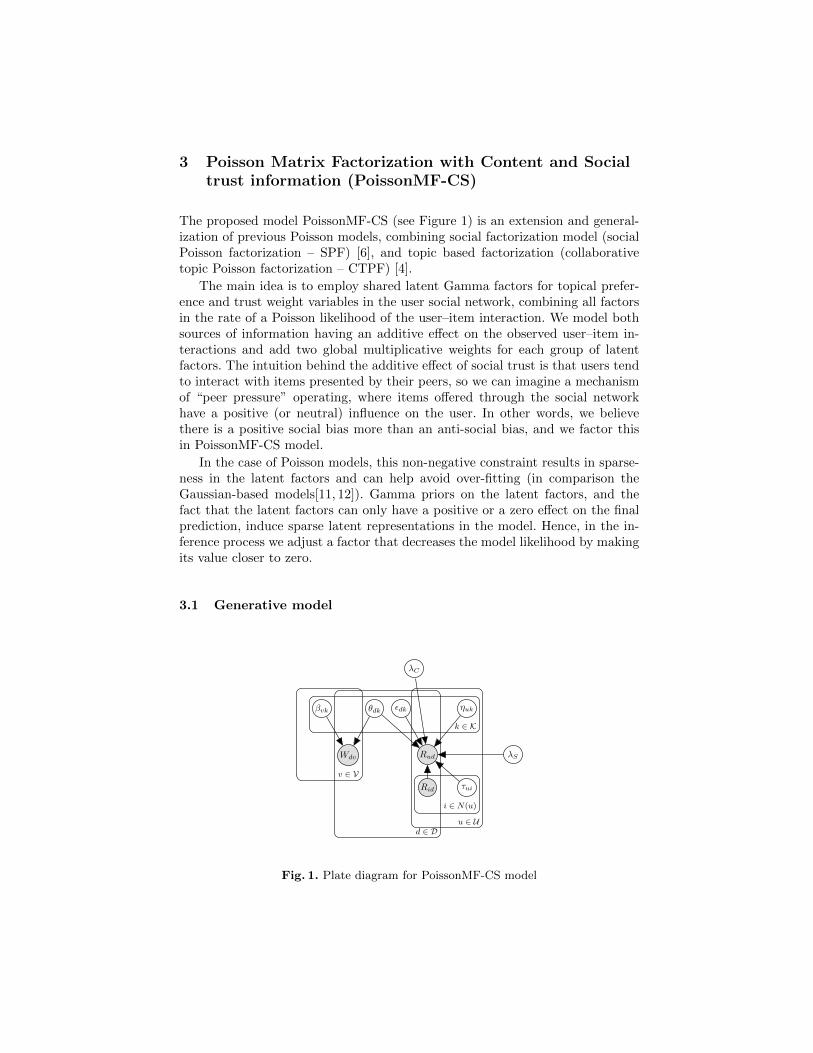
The proposed model PoissonMF-CS (see Figure 1) is an extension and general-ization of previous Poisson models, combining social factorization model (socialPoisson factorization – SPF) [6], and topic based factorization (collaborativetopic Poisson factorization – CTPF) [4].

The main idea is to employ shared latent Gamma factors for topical prefer-ence and trust weight variables in the user social network, combining all factorsin the rate of a Poisson likelihood of the user–item interaction. We model bothsources of information having an additive effect on the observed user–item in-teractions and add two global multiplicative weights for each group of latentfactors. The intuition behind the additive effect of social trust is that users tendto interact with items presented by their peers, so we can imagine a mechanismof “peer pressure” operating, where items offered through the social networkhave a positive (or neutral) influence on the user. In other words, we believethere is a positive social bias more than an anti-social bias, and we factor thisin PoissonMF-CS model.

In the case of Poisson models, this non-negative constraint results in sparse-ness in the latent factors and can help avoid over-fitting (in comparison theGaussian-based models[11, 12]). Gamma priors on the latent factors, and thefact that the latent factors can only have a positive or a zero effect on the finalprediction, induce sparse latent representations in the model. Hence, in the in-ference process we adjust a factor that decreases the model likelihood by makingits value closer to zero.

3.1 Generative model

Rud λS

ηuk

Rid τui

εdkθdk

λC

Wdv

βvk

i ∈ N(u)

u ∈ Ud ∈ D

k ∈ K

v ∈ V

Fig. 1. Plate diagram for PoissonMF-CS model

In this model, Wdv is a counting variable for the number of times word vappears in document d, βv is a latent vector capturing topic distribution ofword v and θd is the document–topic intensity vector, both with dimensionalityK. Count variable Wdv is parametrized by the linear combination of these twolatent factors θTdβv. The document–topic latent factor θd influences also theuser–document rating variable Rud. Each user has a latent vector ηu represent-ing the user–topic propensity, which interacts with the document topic intensityfactor θd and document topic offset factor εd, resulting in the term ηTu θd+ηTu εd.Here, ηTu εd captures the baseline matrix factorization, while ηTu θd connects therating variable with the content-based part of the model (word–document vari-able Wdv). The trust factor τui between user u to user i is equal to zero for allusers that are not connected in the social network ( τui > 0 ⇔ i ∈ N(u)). Thistrust factor adds dependency between social connected users: the user–documentrating Rud is influenced by the average rating to item d given by friends of useru in the social network, weighted by the trust user u assigns to his friends(∑i∈N(u) τuiRid). We model this social dependency using a conditional specified

model, as in [6]. The latent variables λC and λS are weight variables added inthe model to capture and control the general weight of the content and socialfactors. These variables allow us to infer the importance of content and socialfactors according to the dataset or domain of usage. Also, instead of estimatingthese weights from the observed data, we may set λC and λS to constant val-ues, thus controlling the importance of content and social parts of the model.Specifically if we set λC = 0 and λS = 1 we obtain the SPF model, while settingλC = 1 and λS = 0 result in CTPF, and λC = 0 and λS = 0 is equivalent to thesimple Poisson matrix factorization without any side information [11].

Now we present the complete generative model assuming documents (oritems) set D of size |D| = D, vocabulary set V of size |V| = V , users set Uof size |U| = U , the user social network given by the set of neighbors for eachuser {N(u)}u∈U D documents, and K latent factors (topics) (with an index setK).

1. Latent parameter distributions:(a) for all topics k ∈ K:

– for all words v ∈ V: βvk ∼ Gamma(a0β , b0β)

– for all documents d ∈ D: θdk ∼ Gamma(a0θ, b0θ) and εdk ∼ Gamma(a0ε , b

0ε)

– for all users u ∈ U : ηuk ∼ Gamma(a0η, b0η)

• for all user i ∈ N(u): τui ∼ Gamma(a0τ , b0τ )

(b) Content weight: λC ∼ Gamma(a0C , b0C)

(c) Social weight: λS ∼ Gamma(a0S , b0S)

2. Observations probability distribution:(a) for all observed document–word pairs dv :

Wdv|βv,θd ∼ Poisson(βTv θd)

(b) for all observed user–document pairs ud :

Rud|RN(u),d, ηu, εd, θd ∼ Poisson(λCηTu θd + ηTu εd + λS

∑i∈N(u)

τuiRid)

4 Inference

First, we add a set of auxiliary latent Poisson variables to facilitate the posteriorinference of the model. By doing so, the extended model will be complete conju-gate, and consequently have analytical equations for the complete conditionalsand variational updates [16]. In Appendix A we show that those auxiliary vari-ables can be seen as by-product of a lower bound on the expected value of thelog sum of the latent random variables. Variable Ydv,k represent a topic specificlatent count for a word–document pair, so that the observed word–documentcounts is a sum of the latent counts (a property of the Poisson distribution) 1.We can perform a similar modification for the user–item counts, splitting thelatent terms of Rud rate into two groups of topic specific latent count allocationvariables: ZMud,k for the item content part, ZNud,k for the collaborative filtering

part and ZSud,i for the social trust part (for this part, the intuitive explanationfor the latent dimension is the idea of friend specific allocation of trust). Thesum of all those latent counts is the observed user–item interaction count variableRud.

Ydv,k|βvk, θdk ∼ Poisson(βvkθdk)ZMud,k|λC , ηuk, θdk ∼ Poisson(λCηukθdk)

ZNud,k|ηuk, εdk ∼ Poisson(ηukεdk)

ZSud,i|λS , τui, Rid ∼ Poisson(λSτuiRid)

(1)

with∑k

Ydv,k = Wdv, and∑k

ZMud,k + ZNud,k +∑

i∈N(U)

ZSud,i = Rud.

The inference problem consists on the estimation of the posterior distributionof the latent variables given the observed rating R, the observed document–wordcounts W , and the user social network {N(u)}u∈U , in other words, computing

p(Θ|R,W , {N(u)}u∈U ),

where Θ = {β, θ, η, ε, τ, y, z, λC , λS} is the set of all latent variables. The exactcomputation of this posterior probability is intractable for any practical scenario,so we need approximation techniques for efficient parameter learning. In ourcase, we apply variational techniques to derive the learning algorithm. As anintermediate step towards the variational inference algorithm, we also derivethe full conditional distribution for each latent variable. The full conditionaldistribution of each latent variable is also useful as update equations for Gibbssampling, meaning that we could use the resulting equations to implement asampling-based approximation. However, sampling methods are hard to scaleand usually requires more memory, so as a design choice for the implementationof the learning algorithm, we refrained from applying the Gibbs sampling methodand focus on the variational inference.

1 The change consist in assigning a new Poisson variable to each sum-term in thelatent rate of the Poisson likelihood, so if S ∼ Poisson(

∑iXi), we add variables

Si ∼ Poisson(Xi), and by the sum property of Poisson random variable S =∑i Si ∼

Poisson(∑iXi)

In the next sections, we present the full conditional distribution of each ofthe latent variables in Section 4.1, and show the resulting update equation forthe variational parameters in Section 4.2.

4.1 Full conditional distribution

The full conditional distribution of each of the latent variables is the distributionof a variable given all the other variables in the model, except the variable thatwe are considering. Given a set of indexed random variables Xk, we use thenotation p(Xk|X−k) (where X−k means all the variables Xi such that i 6= k) torepresent the full conditional distribution. Given the factorized structure of themodel we can simplify the conditional set to the Markov blanket of the nodewe are considering (children nodes and co-parents nodes)2 [16]. For conciseness,we show the derivations only for one Gamma latent variables and one Poissonlatent count variable.

– Gamma distributed variables: We demonstrate how to obtain the fullconditional distribution for Gamma distributed variable θdk, for the remain-ing Gamma distributed variables we only present the end result without theintermediate steps.

p(θdk|∗) = p(θdk|MarkovBlanket(θdk))

∝ p(θdk)∏Vv=1 p(Ydv,k|βvk, θdk)

∏Uu=1 p(Z

Mud,k|λC , ηuk, θdk)

∝ θa0θ−1dk e−b

0θθdk

∏v θ

Ydv,kdk e−βvkθdk

∏u θ

ZMud,kdk e−λCηukθdk

∝ θa0θ+

∑v Ydv,k+

∑u Z

Mud,k−1

dk e−θdk(b0θ+

∑v βvk+λC

∑u ηuk)

(2)

Normalizing equation Eq. 2 over θdk we obtain the pdf of a Gamma variablewith shape a0θ+

∑v Ydv,k+

∑u Z

Mud,k and rate b0θ+

∑v βvk+λC

∑u ηuk. The

final solution is written in Eq. 3. Also, notice that because of the way themodel is structured all other Gamma latent variable have similar equations,the difference being the set of variables in the Markov blanket.

θdk|∗ ∼ Gamma(a0θ +∑v Ydv,k +

∑u Z

Mud,k, b

0θ +

∑v βvk + λC

∑u ηuk)

βvk|∗ ∼ Gamma(a0β +∑d Ydv,k, b

0β +

∑d θdk)

ηuk|∗ ∼ Gamma(a0η +∑d Z

Mud,k + ZNud,k, b

0η + λC

∑d θdk +

∑d εdk)

εdk|∗ ∼ Gamma(a0ε +∑u−ZNud,k, b0ε +

∑u ηuk)

τui|∗ ∼ Gamma(a0τ +∑d Z

Sud,i, b

0τ + λS

∑dRid)

λC |∗ ∼ Gamma(aC +∑u,d,k Z

Mud,k, bC +

∑u,d,k ηukθdk)

λS |∗ ∼ Gamma(aS +∑u,d,i Z

Sud,i, bS +

∑u,d,i τuiRid)

(3)– Multinomial distributed (auxiliary) variables: looking at the Markov

blanket of Ydv we obtain:

p(Ydv|∗) ∝∏Kk=1 p(Ydv,k|βvk, θdk) =

∏Kk=1 Poisson(Ydv,k|βvkθdk)

∝∏Kk=1

(βvkθdk)Ydv,k

Ydv,k!

(4)

2 We use the notation MarkovBlanket(X) to denote the Markov blanket of a variableX – the set of children and co-parents nodes of variable X in the graphical model

Given that we know that∑k Ydv,k = Wdv, this functional form is equiva-

lent to the pdf of a Multinomial distribution with parameter probabilitiesproportional to βvkθdk.

Ydv|∗ ∼ Mult(Wdv;φdv) with φdv,k =βvkθdk∑k βvkθdk

(5)

Similarly, Zud is a Multinomial with parameters proportional to the parentnodes of Zud. For convenience in the previous section, we split Zud in threeblocks of variables and parameters Zud = [ZMud,Z

Nud,Z

Sud] representing the

different high-level parts of our model. The dimensionality of the first twoblocks is the K, while for the last block is U , resulting that Zud has di-mensionality 2K + U . Similarly the parameters of the Zud full conditionalMultinomial have a block structure ξud = [ξMud, ξ

Nud, ξ

Sud].

Zud|∗ ∼ Mult(Rud; ξud)

with ξud,k =

ξMud,k = λCηukθdk∑

k ηuk(λCθdk+εdk)+λS∑i∈N(u) τuiRid

ξNud,k = ηukεdk∑k ηuk(λCθdk+εdk)+λS

∑i∈N(u) τuiRid

ξSud,i = λSτuiRid∑k ηuk(λCθdk+εdk)+λS

∑i∈N(u) τuiRid

We present in next section how to use these equations to derive a deterministicoptimization algorithm for approximate inference using the variational method.

4.2 Variational inference

Given a family of surrogate distributions q(Θ|Ψ) for the unobserved variables(latent terms) parametrized by variational parameters Ψ , we want to find an as-signment of the variational parameters that minimize the KL-divergence betweenq(Θ|Ψ) and p(Θ|R,W ) 3,

argminΨ

KL{q(Θ|Ψ), p(Θ|R,W )}.

Then, the optimal surrogate distribution can be used as an approximation thetrue posterior. However, the optimization problem using directly the KL di-vergence is not tractable, since it depends on the computation of the evidencelog p(R,W ). This can be accomplished using Jensen inequality to get lowerbounds on the evidence and changing the optimization objective to this lowerbound – the Evidence Lower BOund (ELBO):

argminΨ

L(Ψ) = Eq[log p(R,W , Θ)− log q(Θ|Ψ)]

3 To simplify the notation, we use the short-handed p(Θ|R,W ) to denote the posteriordistribution p(Θ|R,W , {N(u)}u∈U ). Also, we drop the explicitly notation indicatingthe dependency on the social network

Another ingredient in this approximation is the mean field assumption. It con-sists in assuming that all variables in the variational distribution q(Θ|Ψ) aremutually independent. As a result the variational surrogate distribution can beexpressed as a factorized distribution of each latent factor (Eq. 7). Another im-plication is that we can compute the updates for each variational Xi factor usingthe complete conditional of the latent factor [16]. Finally, the inference algorithmconsists in iterative updating of variational parameters of each factorized distri-bution until convergence is reached, resulting in the coordinate ascent variationalinference algorithm based on the following equation:

q(Xi) ∝ exp{Eq[log p(Xi|*)]} (6)

Using Eq. 6, we can take each complete conditional variable that we describedin the previous section and create a respective proposal distribution for thevariational inference. This proposal distribution is in the same family as the fullconditional distribution of the latent variables, meaning that we have a groupof Gamma and Multinomial variables. As long as we update the parameters ofthe variational distribution using Eq. 6, it is guaranteed to minimize the KLdivergence between the surrogate variational distribution (Eq. 7) over the latentvariables and the posterior distribution of the model.

q(Θ|Ψ) = q(λC |aλC , bλC )q(λS |aλS , bλS )∏u,k,i q(τui|aτui , bτui)q(ηuk|aηuk , bηuk)

×∏d,v,k q(εdk|aεdk , bεdk)q(θdk|aθdk , bθdk)q(βvk|aβvk , bβvk)

×∏d,v,u q(Zdv|φ∗dv)q(Yud|ξM∗ud , ξ

N∗ud , ξ

S∗ud )

(7)After applying Eq. 6 together with the expected value properties for each

latent variable4, we obtain the following update equations for the variationalparameters.

– Content and social weights:

aλC = aC +∑u,d,k Rudξ

M∗ud,k, bλC = bC +

∑u,d,k

aηukbηuk

aθdkbθdk

aλS = aS +∑uRudξ

M∗ud,k +

∑vWdvφ

∗dv,k, bλS = bS +

∑u,d,iRid

aτuibτui

– Content v (topic/tags/etc) parameters:

aβvk = a0β +∑dWdvφ

∗dv,k, bβvk = b0β +

∑d

aθdkbθdk

– Item d parameters:

aεdk = a0ε +∑uRudξ

N∗ud,k, bεdk = b0ε +

∑u

aηukbηuk

aθdk = a0θ +∑uRudξ

M∗ud,k +

∑vWdvφ

∗dv,k, bθdk = b0θ + Eq[λC ]

∑u

aηukbηuk

+∑v

aβvkbβvk

– User u parameters:

4 Notice that, if q(X) = Gamma(X|aX , bX) (parameterized by shape and rate) , thenEq[X] = aX

bXand Eq[logX] = Ψ(aX)− log(bX), where Ψ(.) is the Digamma function.

If q(X) = Mult(R|p), then Eq[Xi] = Rpi.

aηuk = a0η +∑dRud(ξ

M∗ud,k + ξN∗ud,k), bηuk = b0η +

∑d Eq[λC ]

aθdkbθdk

+aεdkbεdk

aτui = a0τ +∑dRudξ

S∗ud,i, bτui = b0τ + Eq[λS ]

∑dRid

– item–content dv parameters:

φ∗dv,k ∝ eΨ(aβvk)bβvk

eΨ(aθdk)bθdk

with∑k φdv,k = 1

– user–item ud parameters:

ξM∗ud,k ∝ eEq [log λC ] eΨ(aηuk)bηuk

eΨ(aθdk)bθdk

ξN∗ud,k ∝ eΨ(aηuk)bηuk

eΨ(aεdk)bεdk

ξS∗ud,i ∝ eEq [log λS ] eΨ(aτui )

bτuiRid with

∑k ξ

M∗ud,k + ξN∗ud,k +

∑i ξS∗ud,i = 1

Computing the ELBO: The variational updates calculated in the previoussections are guaranteed to non-decrease the ELBO. However, we still need tocalculate this lower bound after each iteration to evaluate a stopping conditionfor the optimization algorithm. We briefly describe a particular lower-boundingfor the ELBO involving the log-sum present in the Poisson rate.

Note also that the surrogate distribution is factorized using the mean fieldassumptions (Eq. 7), so we have a sum of terms corresponding to the expectedlog probability over the surrogate distribution. The terms comprising the log-probabilities of the Poisson likelihood display a expected value over a sum oflogarithms of latent variables (for example Eq[log(

∑k βvkθdk)]), this is a chal-

lenging computation, but we can apply another lower-bound5 and simplify it toEq. 8.

Eq[log(∑k βvkθdk)] ≥

∑k φ∗dv,k (Eq[log βvk] + Eq[log θdk]])

−∑k φ∗dv,k log φ∗dv,k

(8)

This same simplification can be done to all Poisson terms independentlybecause of the mean field assumptions. It is equivalent to using the auxiliarylatent counts. So, for example, using the latent variable Zdv,k, βvk and θdk, thePoisson term in the ELBO results in Eq. 9.

Eq

[log p(Zdv)

q(Zdv)

]=

∑kWdvφ

∗dv,k Eq[log(βvkθdk)]

−Eq[βvkθdk]−Wdvφ∗dv,k log(φ∗dv,k)− log(Wdv!)

(9)

For the Gamma terms, the calculations are a direct application of ELBO formulafor the appropriate variable. For example, Eq. 10 describes the resulting termsfor βvk.

Eq

[log p(βvk)

q(βvk)

]= log

Γ (aβvk )

Γ (a) + a log b+ aβvk(1− log bβvk)

+(a− aβvk) Eq[log βvk]− bEq[βvk](10)

5 this lower bound is valid for any φ∗dv,k, with∑k φ∗dv,k = 1, check Eq. 13 in Ap-

pendix A for details

Recommendations: Once we learn the latent factors of the model from theobservations we can infer the user preference over the set of items using theexpected value of the user–item rating E[Rud] . The recommendation algorithmranks the unobserved items for each user according to E[Rud] and recommend totop-M items. We utilize the variational distribution to efficiently compute E[Rud]as defined in Eq. 11. This value can be broken down into three non-negativescores: Eq[ηu]T Eq[εd], representing the “classic” collaborative filtering matchingof users preferences and items features, Eq[λC ] Eq[ηu]T Eq[θd] representing thecontent factors contribution and Eq[λS ]

∑i∈N(u) Eq[τui]Rid the social influence

contribution.

E[Rud] ≈ Eq[ηu]T (Eq[λC ] Eq[θd] + Eq[εd]) + Eq[λS ]∑

i∈N(u)

Eq[τui]Rid (11)

Complexity and convergence: the complexity of each iteration of the varia-tional inference algorithm is linear on the number of latent factors K, non-zeroratings nR, non-zero word-document counts nW , users U , items D, vocabularyset W and neighbors for each user nS, in other words O(K(nW +nR+nS+U+D +W )). We have shown that we can obtain closed-form updates for the infer-ence algorithm, which stems from the fact that the model is fully conjugate andin the exponential family of distributions. In this setting variational inferenceis guaranteed to converge, and we observed in the experiments the algorithmconverging after 20 to 40 iterations.

5 Evaluation

In this section, we analyze the predictive power of the proposed model with areal world dataset and compare it with state of the art methods.6

Datasets. to be able to compare with the state-of-art method Correlated TopicRegression with Social Matrix Factorization [5], we conducted experiments usingthe hetrec2011-lastfm-2k (Last.fm) dataset [17]. This dataset consists of a set ofuser–artists weighted interactions (“artists” is item set), a set of user–artists-tagsand a set of user–user relations7. We process the dataset to create an artist–tagsmatrix by summing up all the tags given by all users to a given artist, this matrixis the item–content matrix in our model. Also, we discard the user–artists weight,considering a “1” for all observed cases. After the preprocessing, we sample 85%of the user–artists observation for training, and kept 15% held-out for predictiveevaluation, selecting only users with more than 5 item ratings for the trainingpart of the split.

6 Our C++ implementation of PoissonMF-CS with some of the experiments will beavailable this repository https://github.com/zehsilva/poissonmf_cs

7 The statistics for the dataset are: 1892 users, 17632 artists, 11946 tags, 25434 user–user connections, 92834 user–items interactions, and 186479 user–tag–items entries

50 100 150 200 250# returned items (M)

0.15

0.20

0.25

0.30

0.35

0.40

0.45

0.50

0.55

Avg.

reca

ll@M

PoissonMF-CSCTR-SMFCTRPMF

(a) PoissonMF-CS (K=10) and Gaus-sian based models

50 100 150 200 250# returned items (M)

0.15

0.20

0.25

0.30

0.35

0.40

0.45

0.50

0.55

Avg.

reca

ll@M

Poisson factorization (λC =0,λS =0)SPF (λC =0,λS =1)CTPF (λC =1,λS =0)PoissonMF-CS

(b) PoissonMF-CS (K=10) and otherPF models

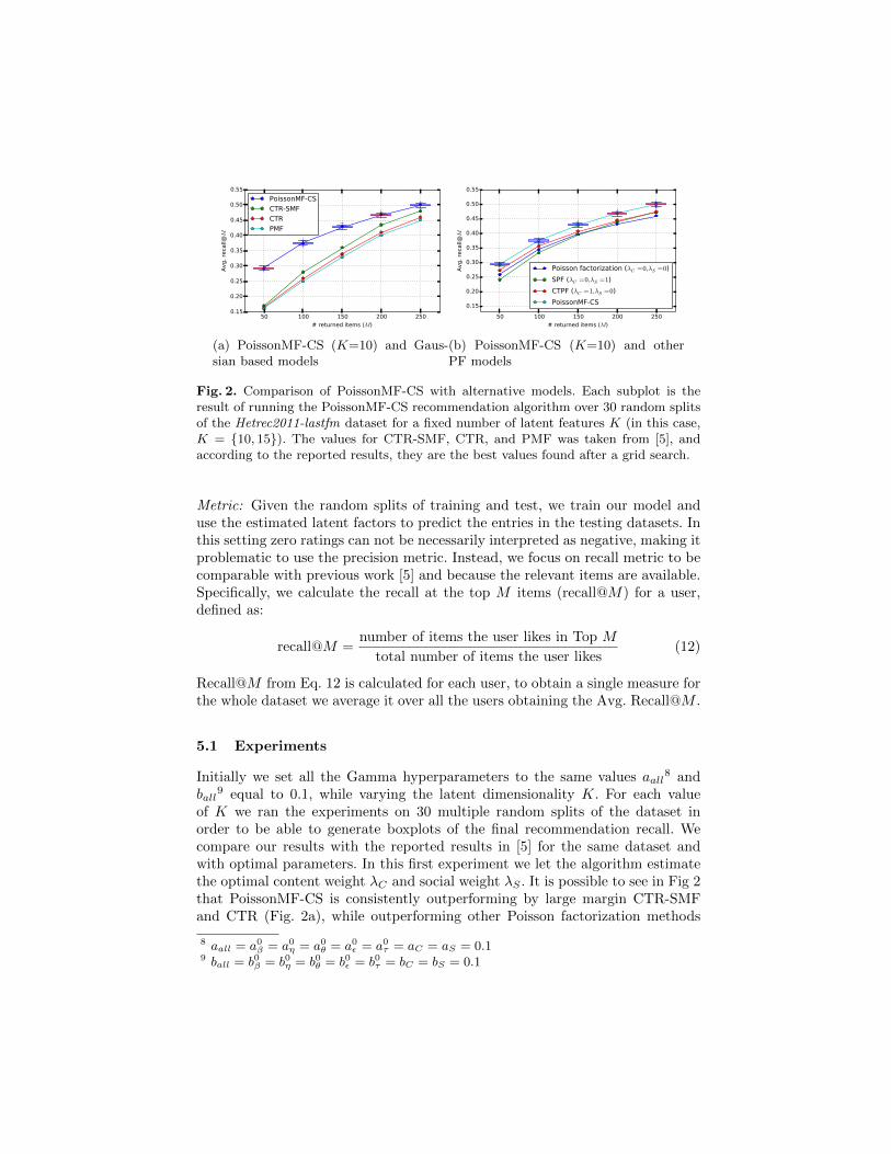
Fig. 2. Comparison of PoissonMF-CS with alternative models. Each subplot is theresult of running the PoissonMF-CS recommendation algorithm over 30 random splitsof the Hetrec2011-lastfm dataset for a fixed number of latent features K (in this case,K = {10, 15}). The values for CTR-SMF, CTR, and PMF was taken from [5], andaccording to the reported results, they are the best values found after a grid search.

Metric: Given the random splits of training and test, we train our model anduse the estimated latent factors to predict the entries in the testing datasets. Inthis setting zero ratings can not be necessarily interpreted as negative, making itproblematic to use the precision metric. Instead, we focus on recall metric to becomparable with previous work [5] and because the relevant items are available.Specifically, we calculate the recall at the top M items (recall@M) for a user,defined as:

recall@M =number of items the user likes in Top M

total number of items the user likes(12)

Recall@M from Eq. 12 is calculated for each user, to obtain a single measure forthe whole dataset we average it over all the users obtaining the Avg. Recall@M .

5.1 Experiments

Initially we set all the Gamma hyperparameters to the same values aall8 and

ball9 equal to 0.1, while varying the latent dimensionality K. For each value

of K we ran the experiments on 30 multiple random splits of the dataset inorder to be able to generate boxplots of the final recommendation recall. Wecompare our results with the reported results in [5] for the same dataset andwith optimal parameters. In this first experiment we let the algorithm estimatethe optimal content weight λC and social weight λS . It is possible to see in Fig 2that PoissonMF-CS is consistently outperforming by large margin CTR-SMFand CTR (Fig. 2a), while outperforming other Poisson factorization methods

8 aall = a0β = a0η = a0θ = a0ε = a0τ = aC = aS = 0.19 ball = b0β = b0η = b0θ = b0ε = b0τ = bC = bS = 0.1

5 10 15 20 50 100#latent factors (K)

0.25

0.26

0.27

0.28

0.29

0.30

0.31

Avg.

reca

ll@M

(M=

50.0

)

(a) M=50

5 10 15 20 50 100#latent factors (K)

0.46

0.47

0.48

0.49

0.50

0.51

0.52

Avg.

reca

ll@M

(M=

250.

0)

(b) M=250

#latent factors (K)0 20 40 60 80 100# returned items (M)

50 100150200250

Avg

reca

ll@M

0.250.300.350.400.450.500.55

0.3000.3250.3500.3750.4000.4250.4500.475

(c) 3D visualization

Fig. 3. Impact of the number of latent variables (K) parameter on the Av. Recall@Mmetric for different number of returned items (M). Each subplot is the result of runningthe PoissonMF-CS recommendation algorithm over 30 random splits of the dataset withK varying in (5,10,15,20,50,100)

0 100 200 300 400 500content λC

0

50

100

150

200

soci

al λS

0.33450.33600.33750.33900.34050.34200.34350.3450

reca

ll@m

=10

0

(a) M=100

0 100 200 300 400 500content λC

0

50

100

150

200

soci

al λS

0.39750.39900.40050.40200.40350.40500.40650.40800.4095

reca

ll@m

=15

0

(b) M=150

Fig. 4. Evaluation of the impact of content and social weight parameters (in all exper-iments in this figure K = 10)

(Fig. 2b) by a significant margin (p ≤ 1 · 10−6 in Wilcoxon paired test for eachM). . This may be indicative that both the choice of Poisson likelihood withnon-negative latent factors and the modelling of content and social weights havepositive impact in the predictive power of the model.

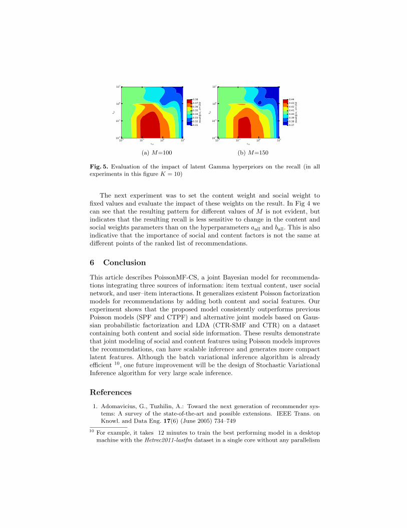
Model selection. Fig. 3 shows the resulting predictive performance of PoissonMF-CS with different values of number of latent factors K in Hetrec2011-lastfmdataset. We concluded that the optimal choice for K is 15. This result is im-portant, indicating that the model is generating compact latent representations,given that the optimal choice of K reported for CTR-SMF in the same datasetis 200. In Fig. 5 we show the results for the latent variable hyperparameters.We ran one experiment varying the hyperparameters aall and ball to understandthe impact of these hyperparameters in the final recommendation. We noticedthat the optimal values for different values of M for both hyperparameters arebetween 0.1 and 1, a result consistent with the recommendations in the liter-ature [12, 4, 6] and with the statistical intuition that Poisson likelihood withGamma prior with shape parameter a < 1 favour sparse latent representation.

10-2 10-1 100 101

aall

10-2

10-1

100

101

b all

0.310.320.330.340.350.360.370.38

reca

ll@M

, M=

100

(a) M=100

10-2 10-1 100 101

aall

10-2

10-1

100

101

b all

0.370.380.390.400.410.420.430.44

reca

ll@M

, M=

150

(b) M=150

Fig. 5. Evaluation of the impact of latent Gamma hyperpriors on the recall (in allexperiments in this figure K = 10)

The next experiment was to set the content weight and social weight tofixed values and evaluate the impact of these weights on the result. In Fig 4 wecan see that the resulting pattern for different values of M is not evident, butindicates that the resulting recall is less sensitive to change in the content andsocial weights parameters than on the hyperparameters aall and ball. This is alsoindicative that the importance of social and content factors is not the same atdifferent points of the ranked list of recommendations.

6 Conclusion

This article describes PoissonMF-CS, a joint Bayesian model for recommenda-tions integrating three sources of information: item textual content, user socialnetwork, and user–item interactions. It generalizes existent Poisson factorizationmodels for recommendations by adding both content and social features. Ourexperiment shows that the proposed model consistently outperforms previousPoisson models (SPF and CTPF) and alternative joint models based on Gaus-sian probabilistic factorization and LDA (CTR-SMF and CTR) on a datasetcontaining both content and social side information. These results demonstratethat joint modeling of social and content features using Poisson models improvesthe recommendations, can have scalable inference and generates more compactlatent features. Although the batch variational inference algorithm is alreadyefficient 10, one future improvement will be the design of Stochastic VariationalInference algorithm for very large scale inference.

References

1. Adomavicius, G., Tuzhilin, A.: Toward the next generation of recommender sys-tems: A survey of the state-of-the-art and possible extensions. IEEE Trans. onKnowl. and Data Eng. 17(6) (June 2005) 734–749

10 For example, it takes 12 minutes to train the best performing model in a desktopmachine with the Hetrec2011-lastfm dataset in a single core without any parallelism

2. Tang, J., Hu, X., Liu, H.: Social recommendation: a review. Social NetworkAnalysis and Mining 3(4) (2013) 1113–1133

3. Wang, C., Blei, D.M.: Collaborative topic modeling for recommending scientificarticles. In: Proceedings of the 17th ACM SIGKDD International Conference onKnowledge Discovery and Data Mining, San Diego, CA, USA, August 21-24, 2011.(2011) 448–456

4. Gopalan, P., Charlin, L., Blei, D.M.: Content-based recommendations with poissonfactorization. In: Advances in Neural Information Processing Systems 27: AnnualConference on Neural Information Processing Systems 2014, December 8-13 2014,Montreal, Quebec, Canada. (2014) 3176–3184

5. Purushotham, S., Liu, Y.: Collaborative topic regression with social matrix fac-torization for recommendation systems. In: Proceedings of the 29th InternationalConference on Machine Learning, ICML 2012, Edinburgh, Scotland, UK, June 26- July 1, 2012, icml.cc / Omnipress (2012)

6. Chaney, A.J., Blei, D.M., Eliassi-Rad, T.: A probabilistic model for using socialnetworks in personalized item recommendation. In: Proceedings of the 9th ACMConference on Recommender Systems, RecSys 2015, Vienna, Austria, September16-20, 2015. (2015) 43–50

7. Ma, H., Zhou, D., Liu, C., Lyu, M.R., King, I.: Recommender systems with socialregularization. In: Proceedings of the Forth International Conference on WebSearch and Web Data Mining, WSDM 2011, Hong Kong, China, February 9-12,2011. (2011) 287–296

8. Yuan, Q., Chen, L., Zhao, S.: Factorization vs. regularization: Fusing heterogeneoussocial relationships in top-n recommendation. In: Proceedings of the Fifth ACMConference on Recommender Systems. RecSys ’11, New York, NY, USA, ACM(2011) 245–252

9. Kang, J., Lerman, K.: LA-CTR: A limited attention collaborative topic regressionfor social media. In: Proceedings of the Twenty-Seventh AAAI Conference onArtificial Intelligence, July 14-18, 2013, Bellevue, Washington, USA. (2013)

10. Wang, H., Chen, B., Li, W.: Collaborative topic regression with social regulariza-tion for tag recommendation. In: IJCAI 2013, Proceedings of the 23rd InternationalJoint Conference on Artificial Intelligence, Beijing, China, August 3-9, 2013. (2013)2719–2725

11. Gopalan, P., Hofman, J.M., Blei, D.M.: Scalable recommendation with hierarchicalpoisson factorization. In Meila, M., Heskes, T., eds.: Proceedings of the Thirty-First Conference on Uncertainty in Artificial Intelligence, UAI 2015, July 12-16,2015, Amsterdam, The Netherlands, AUAI Press (2015) 326–335

12. Gopalan, P., Ruiz, F.J.R., Ranganath, R., Blei, D.M.: Bayesian nonparametricpoisson factorization for recommendation systems. In: Proceedings of the Seven-teenth International Conference on Artificial Intelligence and Statistics, AISTATS2014, Reykjavik, Iceland, April 22-25, 2014. Volume 33 of JMLR Workshop andConference Proceedings., JMLR.org (2014) 275–283

13. Hu, C., Rai, P., Chen, C., Harding, M., Carin, L.: Scalable bayesian non-negativetensor factorization for massive count data. In: Machine Learning and Knowl-edge Discovery in Databases - European Conference, ECML PKDD 2015, Porto,Portugal, September 7-11, 2015, Proceedings, Part II. (2015) 53–70

14. Hu, C., Rai, P., Carin, L.: Non-negative matrix factorization for discrete data withhierarchical side-information. In: Proceedings of the 19th International Conferenceon Artificial Intelligence and Statistics, AISTATS 2016, Cadiz, Spain, May 9-11,2016. (2016) 1124–1132

15. Acharya, A., Teffer, D., Henderson, J., Tyler, M., Zhou, M., Ghosh, J.: Gammaprocess poisson factorization for joint modeling of network and documents. In:Machine Learning and Knowledge Discovery in Databases - European Conference,ECML PKDD 2015, Porto, Portugal, September 7-11, 2015, Proceedings, Part I.(2015) 283–299

16. Bishop, C.M.: Pattern Recognition and Machine Learning (Information Scienceand Statistics). Springer-Verlag New York, Inc., Secaucus, NJ, USA (2006)

17. Cantador, I., Brusilovsky, P., Kuflik, T.: 2nd workshop on information heterogene-ity and fusion in recommender systems (hetrec 2011). In: Proceedings of the 5thACM conference on Recommender systems. RecSys 2011, New York, NY, USA,ACM (2011)

A A lower bound for Eq[log∑

kXk]

The function log(·) is a concave, meaning that:

log(px1 + (1− p)x2) ≥ p log x1 + (1− p) log x2∀p : p ≥ 0

By induction this property can be generalized to any convex combination of xk(∑k pkxk with

∑k pk = 1 and pk ≥ 0): log

∑k pkxk ≥

∑k pk log xk Now using

random variables we can create a similar convex combination by multiplying anddividing each random variable Xk by pk > 0 and apply the sum of of expectationproperty:

Eq[log∑kXk] = Eq[

∑k log pk

Xkpk

]

log∑k pk

Xkpk≥

∑k pk log Xk

pk

⇒ Eq[log∑k pk

Xkpk

] ≥∑k pk Eq[log Xk

pk]

⇒ Eq[log∑kXk] ≥

∑k pk Eq[logXk]− pk log pk

(13)

The lower bound of Eq. 13 is applied in Eq. 8 and it is a general lower bounduseful for the log–sum terms in the ELBO computation. If we want a tight lowerbound, we should use Lagrange multipliers to choose the set of pk that maximizethe lower-bound given that they sum to 1.

L(p1, . . . , pK) = (∑k pk Eq[logXk]− pk log pk) + λ (1−

∑k pk)

∂L∂pk

= Eq[logXk]− log pk − 1− λ = 0∂L∂λ = 1−

∑k pk = 0

⇒ Eq[logXk] = log pk + 1 + λ⇒ exp Eq[logXk] = pk exp(1 + λ)

⇒∑k exp Eq[logXk] =

∑k

pk︸ ︷︷ ︸=1

exp(1 + λ)

⇒ pk =exp{Eq [logXk]}∑k exp{Eq [logXk]}

(14)

The final formula for pk in Eq. 14 is exactly the same that we can find forthe parameters of the Multinomial distribution of the auxiliary variables in thePoisson model with sum of Gamma distributed latent variables, which demon-strates that the choice of distribution for the auxiliary variables is optimal forthis lower-bound.