The Scientific Context of Quality Improvement1987 by George E. P. Box and Søren Bisgaard.

Practical Significance

We need to find out how to make products better and cheaper. Modern Quality Improvement does this by employing techniques ranging from the very simple to the more sophisticated in a never-ending effort to learn more about the product and the process. Its driving force is scientific method, disseminated throughout the company.

Simple tools widely applied are essential for refining and improving a product which is actually being manufactured. But they can compensate only partially for flaws which, because of faulty design, may have been built into the product and the process in the development stages. Thus in the development stages of product and process, experimenting with alternatives is essential to ensure that basic designs are right. Such experimentation is usually expensive and to achieve maximum efficiency must be done using Statistical Experimental Design.

The contributions from Japan of Genichi Taguchi are discussed and explained. Results of the latest research at the Center for Quality and Productivity at the University of Wisconsin - Madison show how Taguchi's good engineering ideas can be used while substituting, where appropriate, simpler and more efficient statistical procedures.

Keywords: Statistics, Design of Experiments, Productivity

Introduction

The United States is facing a serious economic problem. Its role as the world's most powerful industrial nation is being threatened. Wheelwright (1984) provides a list compiled originally by Professor Robert B. Reich of Harvard University which is just one of many indicators of the seriousness of this problem.

Automobiles

Cameras

Stereo Components

Medical Equipment

Color Television Sets

Hand Tools

Radial Tires

Electric Motors

Food Processors

Microwave Ovens

Athletic Equipment

Computer Chips

Industrial Robots

Electron Microscopes

Machine Tools

He points out that "in all of these industries. U.S. worldwide manufacturing share has slipped by at least 50% in the last decade". An important part of this share has gone to Japan. It is clear that the Japanese are doing something right. The important question is, "What is it?" The answer, of course, is that they are doing a number of things, but a major reason for their competitive edge in high-quality, low-cost products is that they use statistical methods. Quite simply the Japanese have a secret ingredient:

They Do It and We Don't

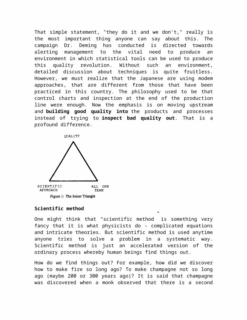
That simple statement, "they do it and we don't," really is the most important thing anyone can say about this. The campaign Dr. Deming has conducted is directed towards alerting management to the vital need to produce an environment in which statistical tools can be used to produce this quality revolution. Without such an environment, detailed discussion about techniques is quite fruitless. However, we must realize that the Japanese are using modem approaches, that are different from those that have been practiced in this country. The philosophy used to be that control charts and inspection at the end of the production line were enough. Now the emphasis is on moving upstream and building good quality into the products and processes instead of trying to inspect bad quality out. That is a profound difference.

Scientific method

One might think that “scientific method” is something very fancy that it is what physicists do - complicated equations and intricate theories. But scientific method is used anytime anyone tries to solve a problem in a systematic way. Scientific method is just an accelerated version of the ordinary process whereby human beings find things out.

How do we find things out? For example, how did we discover how to make fire so long ago? To make champagne not so long ago (maybe 200 or 300 years ago)? It is said that champagne was discovered when a monk observed that there is a second fermentation that can take place in wine. Now this second fermentation must have been occurring ever since people began to make wine, thousands of years ago. Yet it was not until comparatively recently that anyone noticed the second fermentation and thought about using it.

Producing good quality and increasing productivity at low cost is achieved by learning about processes. This was clearly Shewhart's (1939) intention when he said, “The three steps (specification, production, and judgment of quality) constitute a dynamic scientific process of acquiring knowledge...mass production viewed in this way constitutes a continuing and self-corrective method for making the most efficient use of raw and fabricated materials.” He never intended quality control to be just passive inspection.

So what are the essential elements in discovering something? We need two things. We need a critical event, one that contains significant information, like the second fermentation. But no one is going to see the critical event, no one is going to exploit it unless there is a perceptive observer present. These two things, a critical event and a perceptive observer, are essential.

Most events are not critical. There is not much to be learned (from them. They are just part of the ordinary things that happen all the time. But every now and then

something happens that we could learn from. These events are comparatively rare. Perceptive observers are rare too. Ideally they need to possess not only natural curiosity but also training in the relevant area of expertise. Hence we are dealing with the coming together of two rare occurrences. If we rely entirely on chance, the probability of these two coming together is very small. That is why when we look back in history to say the 12th, 13th and 14th centuries. We see that technological change occurred very slowly. For example over a hundred years the design of sailing ships changed, but no by very much.

Around 300 years ago technological change started to occur much more rapidly. One of the primary reasons was the use of scientific method, which increased the probability of a critical event and a perceptive observer coming together. There are two ways to achieve this. One is to make sure that naturally occurring informative events are brought to the attention of a perceptive observer, and the other is to increase the chance of an informative event actually occurring. We will call the first informed observation and the second directed experimentation.

Informed Observation

As an example of informed observation suppose we were interested in studying solar eclipses and we knew that one was going to occur and that the best location to see it was in southern Australia. To increase the probability of learning from the eclipse we would be sure to arrange for people knowledgeable about astronomy and solar eclipses to be in southern Australia at the right time, equipped with the necessary instruments to make meaningful observations. That is what we mean by increasing the probability that a naturally occurring event would be observed and appreciated by a perceptive observer.

A quality control chart serves the same purpose. People knowledgeable about the process look at it and say, “What the heck happened at point X?”

In the words of Walter Shewhart, they look for an assignable cause. With a quality control chart, data from the process is not buried in a notebook, a file drawer, or a computer file. No, the charts are put up on the wall where the people who are most involved with the process can see them and can reason about them. A system is created that ensures that when a critical event may have occurred as indicated by a point outside the control limits or some unusual pattern, the people who know about the process can observe this, ask what happened. And take action. “If that is where Joe spat in the batch, then let us change the system so Joe cannot spit in the batch anymore.” In this way the people working with a system can slowly eliminate the bugs and create a process of continuous, never-ending improvement.

Every process generates information that can be used to improve it. This is perhaps quite simple to see when the process is a machine. But the philosophy applies equally to a hospital ward, to customer billing, to a typing pool, and to a maintenance garage (see Hunter, O'Neill and Wallen, 1986). Every job has a process in it, and every process generates information that can be used to improve it.

Tools for Observation

One can complain about why it takes a typing pool so long to type documents. But Dr. Deming tells us that it is useless just to grumble at people. Management must provide employees with tools that will enable them to do their jobs better, and with encouragement to use these tools. In particular, they must collect data. How long do typing pool documents sit around waiting? How long does it take to type them? How are they being routed? How much delay is caused by avoidable corrections? How often are letters unnecessarily labeled “urgent”?

Professor Ishikawa, in Japan, has put together one such excellent set of tools that help people get at the information that is being generated ail the time by processes. He calls them “The Seven Tools” and they are check sheets, the Pareto chart (originally due to Dr. Juran), the cause-and-effect diagram, histograms,

stratification, scatter plots, and graphs (in which he includes control charts). All are simple and everybody can use them.

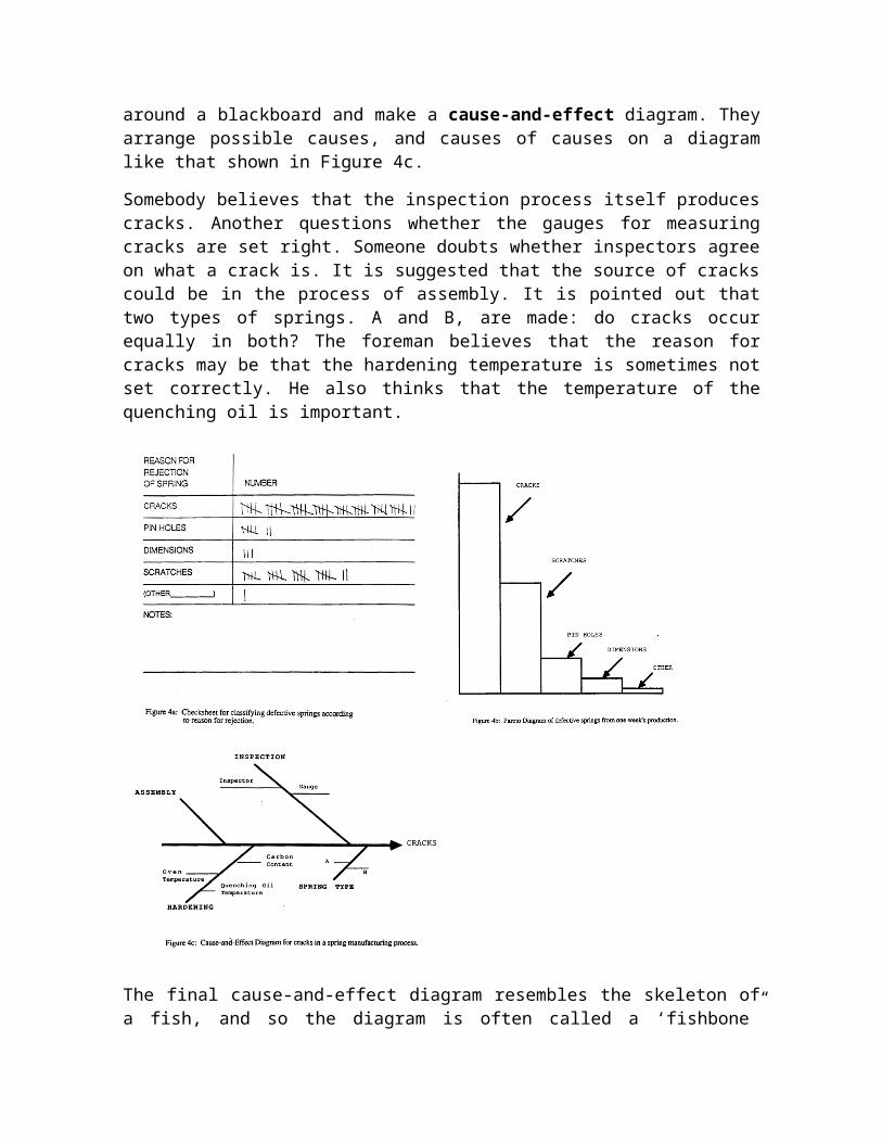
Let us illustrate some of these tools and show how they might be used to examine a problem. Suppose we find in one week's production of springs, that 75 were defective. That is informative but not of much help for improving the process. But suppose we go through all the defective springs and categorize them into those having defects because of cracks, because of scratches, because of pin holes, because the dimensions were not right, and so on, marking off these items on the check sheet in Figure 4a. The results can then be displayed using the Pareto chart in Figure 4b. In this particular instance 42 out of the 75 springs were discarded because of cracks.

Clearly cracks are an important problem. Pareto charts focus attention on the most important things to work on. They separate the vital few from the trivial many (Juran, 1964).

These tools and the use of data allow anyone in the organization, high or low, to deal with the “heavy-weight authority” who says, “I can tell you what the problem is. My experience tells me that the main cause of rejects is pin holes. That's what we should work on.” That is his opinion but it is in this instance wrong. The data say the biggest problem is with cracks. Whoever he is, he must be told, ‘Show me the data!”

The next thing is to figure out what could be causing the cracks. The people who make the springs should get together around a blackboard and make a cause-and-effect diagram. They arrange possible causes, and causes of causes on a diagram like that shown in Figure 4c.

Somebody believes that the inspection process itself produces cracks. Another questions whether the gauges for measuring cracks are set right. Someone doubts whether inspectors agree on what a crack is. It is suggested that the source of cracks could be in the process of assembly. It is pointed out that two types of springs. A and B, are made: do cracks occur equally in both? The foreman believes that the reason for cracks may be that the hardening temperature is sometimes not set correctly. He also thinks that the temperature of the quenching oil is important.

The final cause-and-effect diagram resembles the skeleton of a fish, and so the diagram is often called a ‘fishbone” chart. Its main function is to facilitate focused brainstorming, argument, and discussion among people about what might cause the cracks. Often some of the possibilities can be eliminated right away by simply talking them over.

Usually there will be a number of possibilities left and it is not known which items cause which problems. Using data coming from the process we can often sort out the different possibilities with the Seven Tools.

Suppose, for example, we have categorized the cracks by size. The histogram shown in Figure 4d can then be used to show how many cracks of different sizes occurred. This is of value in itself for conveniently summarizing the crack size problem we are facing. But much more can be learned by splitting or stratifying the histogram in various ways.

For example, the fact that there are two types of springs provides an opportunity for stratification. In Figure 4e the original histogram has been split into two, one for springs of type A, and one for the springs of type B. k is evident not only that most

of the cracks are in springs of type A but also that the size of the type A cracks are on the average larger and that the spread is greater. So now we ask, “What's special about type A springs?” if we knew who inspected what, we could also stratify the data by inspectors and see if there are differences between inspectors.

Scatter diagrams can also be helpful. If it is known that hardening temperature varies quite a bit, one might plot the crack size against the hardening temperature. For example, Figure 4f suggests some kind of relationship between crack size and hardening temperature or a common factor affecting both. A control chart recording the oven temperature can tell us how stable the temperature is over the and whether a higher frequency of cracks is associated with any patterns in the temperature recorded.

Clearly these seven tools are really very commonsensical and very powerful things. By helping people to see how often things happen, when they happen, where they happen, and when they are different, the workforce can be trained to be quality detectives producing never-ending improvements. This will always overtake any system relying on quality policing through inspection, which primarily attempts to maintain the status quo.

Does it Work in the United States?

People often ask. “Will this work in the USA?" An interesting example is provided by a Japanese manufacturer of television sets and other electronic devices that some years ago purchased an American television plant just outside Chicago. When Japanese management first took over, the reject rare was 146 percent. That may sound extraordinary. It means that roost television sets were pulled off the line to be repaired at least once and some were pulled off twice. By using tools like the ones described above, the reject rate was brought down to 2 percent. The change did not, of course, happen overnight. It took four or five years of meticulously weeding out of the causes of defects. However, when a study group from the University of Wisconsin led by the late Professor William O. Hunter, visited the plant in the Spring of 1985, there were no Japanese in sight. Only Americans were employed. When asked, there seemed no question that the employees liked the new system better. The managers said that the plant was a madhouse before. They could not find any time to manage because they were always putting out fires. With a 146 percent reject rate practically every television set had to be fixed individually. The benefits of the changes were a dramatically improved quality product, higher productivity, greatly improved morale, and the managers got time to manage.

Directed Experimentation

Informed observation is not enough in itself because no amount of fine-tuning can overcome fundamental flaws in products and processes due to poor design. Directed experimentation, the other component of the scientific method that we discussed earlier, is needed to ensure that we have excellently designed products and processes to begin with. Only by designing quality into the products and processes can the Levels of quality and productivity we see in Japan be achieved.

It used to be that quality control was thought to concern only the downstream side of the process, using control charts and inspection schemes. Now the emphasis is on moving upstream focusing attention on getting a product and a process that are sufficiently well-designed so that seldom is anything produced of unsatisfactory quality. This reduces the need for inspection, and great economic gains are achieved. This push for moving upstream, already strongly recommended fifty years ago by Egon Pearson (1935), is embodied in the Japanese approach. To reach this goal directed experimentation is needed.

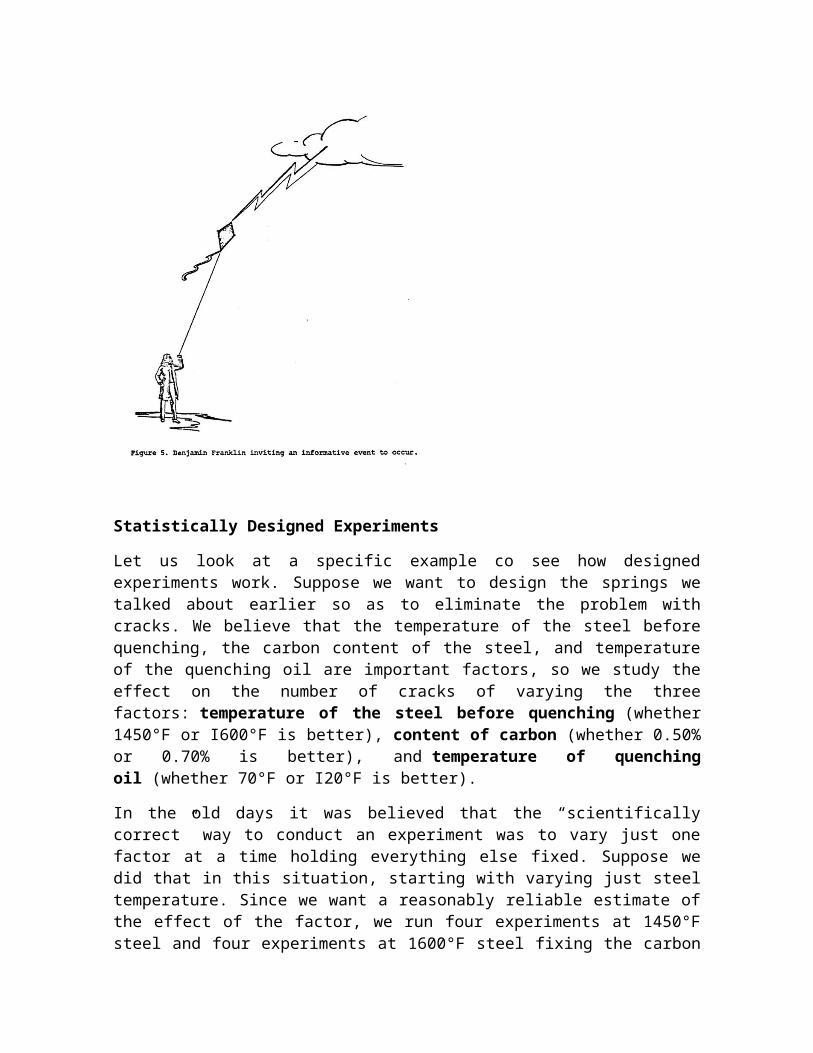
Figure 5 shows a somewhat simplified version of Benjamin Franklin's famous experiment that established the connection between electricity and lightning. By flying a kite in a lightning cloud he clearly invited an informative event to occur.

On a recent study mission to Japan, researchers from the Center for Quality and Productivity Improvement at Wisconsin and AT&T Bell Laboratories were shown a new copying machine. This splendid machine can produce copies of almost any size at an enormous rate. It had taken the company three years to design it and the chief design engineer told us that 49 designed experiments, many of which had involved more than 100 experimental runs, had been conducted to get the machine the way it is. Many of those experiments were aimed at making the copy machines robust to all the things that could happen to them when they were exported all over the world and exposed to use in all sorts of adverse conditions. The manufacturer's objective was to make a machine that would produce good copies no matter whether there was high humidity, low humidity, high temperature, low temperature, thin paper, thick paper, and so on. It took a lot of effort to get the engineering design right, but now they have developed a copier chat will very seldom fail or give trouble and that is its own advertisement.

What is experimental design? Statistical experimental design was invented in the early 1920s by R. A. Fisher in England. In her biography, Joan Fisher Box (1978) describes the work of Fisher. In 1919 he went to work at a small, at that time not very well known, agricultural research station called Rothamsted about forty miles north of London. The workers at Rothamsted were interested in finding out the best way to grow wheat, potatoes, barley, and other crops. They could have conducted their experiments in a greenhouse, carefully controlling the temperature and humidity, making artificial soil that was uniform, and keeping out the birds. By doing so they would have produced results that applied to plants grown under these very artificial conditions. However, the results would most likely have been entirely useless in deciding what would happen on a farmer's field.

 The question, then, was how to run experiments in the "noisy" and imperfectly controlled conditions of the real world. Fisher showed how to do it and his ideas were quickly adopted worldwide, particularly in the United States. This is perhaps

one reason why at least one American industry, namely agriculture, still leads the world.

It was gradually realized that Fisher's work on experimental method constituted a major step forward in human progress and that his results were by no means confined co agriculture. He showed for the first time how experimentation could be moved out of the laboratory. His methods quickly produced relevant, practical findings in a multitude of important fields, including medicine, education, and biology. In particular, his ideas were suitably developed for the industrial setting (see, for example. Box and Wilson, 1951; Davies, 1954; Daniel, 1976: Box, Hunter and Hunter 1978; and Box and Draper. 1987) and over the years many statically designed experiments have been run in industry in the United States, Great Britain, and many other countries. Statistical design is an extremely potent tool and when employed it has almost invariably been successful. Unfortunately, application has been very patchy in the West usually because of a lack of management understanding and support. In Japan, on the other hand, management requiresthat such methods be used to develop high quality products and processes that will rarely go wrong.

Statistically Designed Experiments

Let us look at a specific example co see how designed experiments work. Suppose we want to design the springs we talked about earlier so as to eliminate the

problem with cracks. We believe that the temperature of the steel before quenching, the carbon content of the steel, and temperature of the quenching oil are important factors, so we study the effect on the number of cracks of varying the three factors: temperature of the steel before quenching (whether 1450°F or I600°F is better), content of carbon (whether 0.50% or 0.70% is better), and temperature of quenching oil (whether 70°F or I20°F is better).

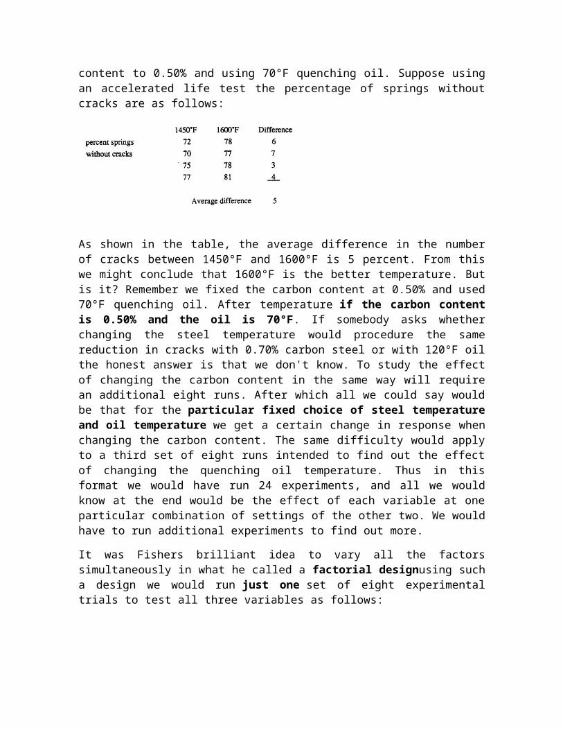
In the old days it was believed that the “scientifically correct” way to conduct an experiment was to vary just one factor at a time holding everything else fixed. Suppose we did that in this situation, starting with varying just steel temperature. Since we want a reasonably reliable estimate of the effect of the factor, we run four experiments at 1450°F steel and four experiments at 1600°F steel fixing the carbon content to 0.50% and using 70°F quenching oil. Suppose using an accelerated life test the percentage of springs without cracks are as follows:

As shown in the table, the average difference in the number of cracks between 1450°F and 1600°F is 5 percent. From this we might conclude that 1600°F is the better temperature. But is it? Remember we fixed the carbon content at 0.50% and used 70°F quenching oil. After temperature if the carbon content is 0.50% and the oil is 70°F. If somebody asks whether changing the steel temperature would procedure the same reduction in cracks with 0.70% carbon steel or with 120°F oil the honest answer is that we don't know. To study the effect of changing the carbon content in the same way will require an additional eight runs. After which all we could say would be that for the particular fixed choice of steel temperature and oil temperature we get a certain change in response when changing the carbon content. The same difficulty would apply to a third set of eight runs intended to find out the effect of changing the quenching oil temperature. Thus in this format we would have run 24 experiments, and all we would know at the end would be the effect of each variable at one particular combination of settings of the other two. We would have to run additional experiments to find out more.

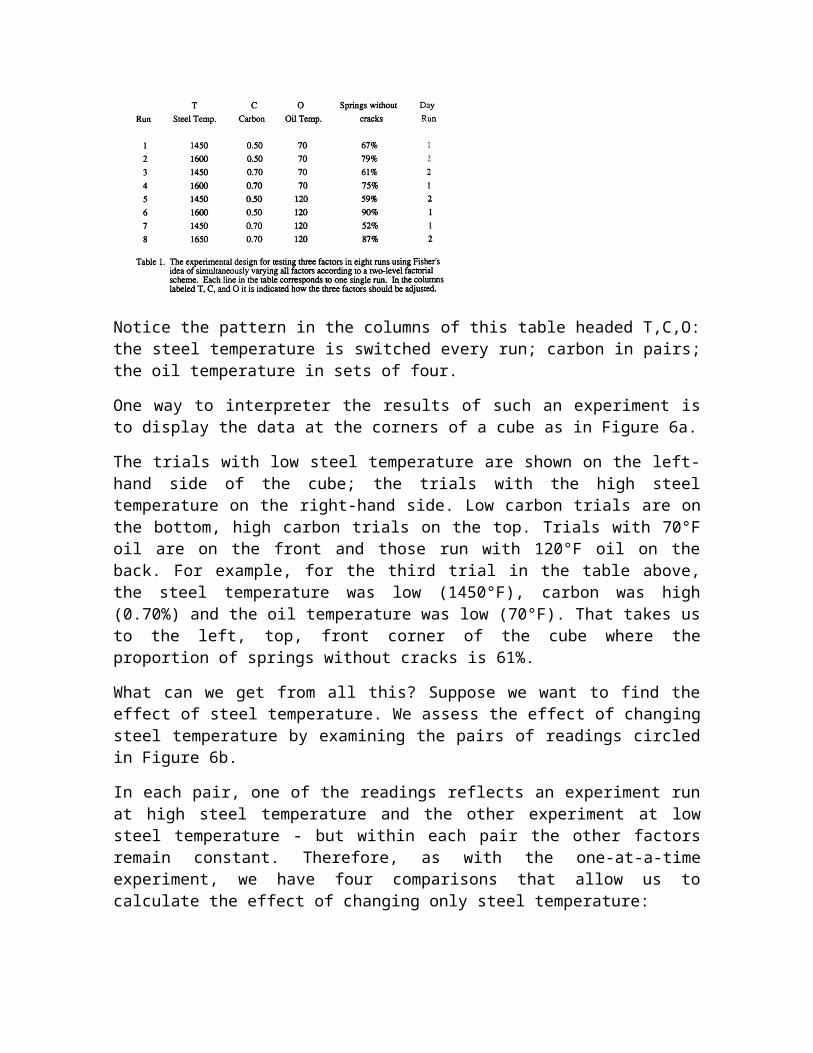
It was Fishers brilliant idea to vary all the factors simultaneously in what he called a factorial designusing such a design we would run just one set of eight experimental trials to test all three variables as follows:

Notice the pattern in the columns of this table headed T,C,O: the steel temperature is switched every run; carbon in pairs; the oil temperature in sets of four.

One way to interpreter the results of such an experiment is to display the data at the corners of a cube as in Figure 6a.

The trials with low steel temperature are shown on the left-hand side of the cube; the trials with the high steel temperature on the right-hand side. Low carbon trials are on the bottom, high carbon trials on the top. Trials with 70°F oil are on the front and those run with 120°F oil on the back. For example, for the third trial in the table above, the steel temperature was low (1450°F), carbon was high (0.70%) and the oil temperature was low (70°F). That takes us to the left, top, front corner of the cube where the proportion of springs without cracks is 61%.

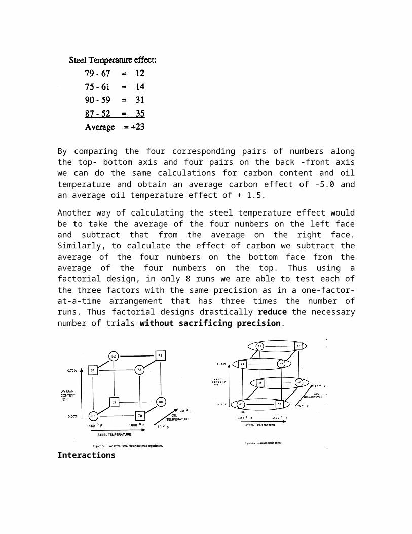
What can we get from all this? Suppose we want to find the effect of steel temperature. We assess the effect of changing steel temperature by examining the pairs of readings circled in Figure 6b.

In each pair, one of the readings reflects an experiment run at high steel temperature and the other experiment at low steel temperature - but within each pair the other factors remain constant. Therefore, as with the one-at-a-time experiment, we have four comparisons that allow us to calculate the effect of changing only steel temperature:

By comparing the four corresponding pairs of numbers along the top- bottom axis and four pairs on the back -front axis we can do the same calculations for carbon content and oil temperature and obtain an average carbon effect of -5.0 and an average oil temperature effect of + 1.5.

Another way of calculating the steel temperature effect would be to take the average of the four numbers on the left face and subtract that from the average on the right face. Similarly, to calculate the effect of carbon we subtract the average of the four numbers on the bottom face from the average of the four numbers on the top. Thus using a factorial design, in only 8 runs we are able to test each of the three factors with the same precision as in a one-factor-at-a-time arrangement that has three times the number of runs. Thus factorial designs drastically reduce the necessary number of trials without sacrificing precision.

Interactions

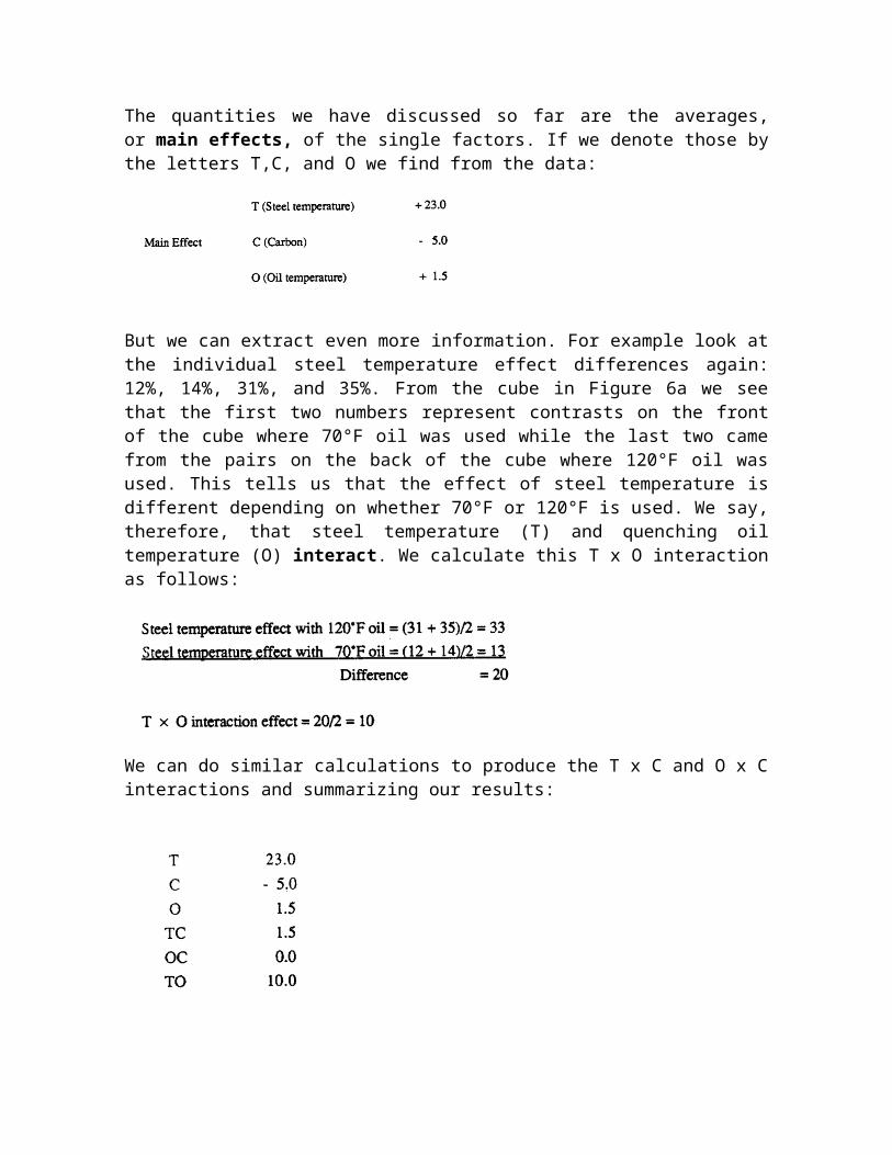
The quantities we have discussed so far are the averages, or main effects, of the single factors. If we denote those by the letters T,C, and O we find from the data:

But we can extract even more information. For example look at the individual steel temperature effect differences again: 12%, 14%, 31%, and 35%. From the cube in Figure 6a we see that the first two numbers represent contrasts on the front of the cube where 70°F oil was used while the last two came from the pairs on the back of the cube where 120°F oil was used. This tells us that the effect of steel temperature is different depending on whether 70°F or 120°F is used. We say, therefore, that steel temperature (T) and quenching oil temperature (O) interact. We calculate this T x O interaction as follows:

We can do similar calculations to produce the T x C and O x C interactions and summarizing our results:

This single eight-run design has not only allowed us to estimate all the main effects with maximum precision, it has also enabled us to determine the three interactions between pairs of factors. This would have been impossible with the one-factor-at-a-time design.Blocking and Randomization

The practical engineer might, with reason, have reservations about process experimentation of any kind because in his experience processes do not always remain stable or in statistical control. For example, the oil used for quenching deteriorates with use. Steel, while having the same carbon content may have other properties that vary from batch to batch. He might therefore conclude that his process is too complex for experimentation to be useful.

However, what could be more complicated and noisy than the agricultural environment in which Fisher conducted his experiments? The soil was different from one corner of the field to another, some parts of the field were in shade while others were better exposed to the Sun, and some areas were wetter than others. Sometimes birds would eat the seeds in a particular part of the field. All such influences could bias the experimental results.

Fisher used blocking to eliminate the effect of inhomogeneity in the experimental material andrandomization to avoid confounding with unknown factors.

To explain the idea of blocking supposes with the above experiment that only four experimental runs could be made in a single day. The experiments would then

have to be run on two different days. 1f there was a day-to-day difference, this could bias the results.

Suppose however we ran the eight runs in the manner shown in Figure 6a (see also Table 1) where the data shown in circles were obtained on day 1 and the data shown in squares were obtained on day 2.

Notice that there are two runs on the left-hand side and two runs on the right-hand side of the cube that were made in the first day. Similarly there are two runs on the left-hand side of the cube and two runs on the right-hand side of the cube that was made on the second day.

With this balanced arrangement, any systematic difference between days will cancel out when we calculate the steel temperature effect. A similar balance occurs for the other two main effects and even for the interactions.

A skeptical reader could add 5 to all the numbers marked as squares on the cube pretending that the process level changed from one day to the next by that amount. He will find that recalculation of all the main effects and interactions would produce the same results as before. As one can see, the beauty of Fisher's method of blocking is that it allows us to run the experiment in such a way that inhomogeneities such as day-to-day, machine-to-machine, batch-to-batch, and shift-to-shift differences can be balanced out and eliminated. The practical significance is that effects are determined with much greater precision. Without blocking, important effects could be missed or it would take many more experiments to find them.

It might me as if, by blocking, we have gained the possibility of running experiments in a non-stationary environment at no cost. However, this is not quite true. From an eight run experiment one can calculate at most eight quantities: the mean of all the runs, three main effects, three two-factor interactions and a three-factor interaction. Using this arrangement we have associated the block difference with the contrast corresponding to the three-factor interaction. Thus these two effects are deliberately mixed up, or in statistical language the block effect and the three-factor interaction are confounded. In many examples, however the three-factor interaction will be unimportant.

What about unsuspected trends and patterns that happen within a block of experimental runs? Fisher's revolutionary idea was to assign the individual treatment combinations in random order within the blocks. In our example, the four runs made on day 1 would be run in a random order and the four runs made on day 2 would also be run in a random order. In this way the experimenter can guard himself against the possibility of unsuspected patterns biasing the results.

These ideas of factorial and other special designs, of running experiments in small blocks, of randomization, and where necessary, replication, provided for the first time a method for running planned experiments in a real world environment, which was fully in statistical control.

Fractional Designs

If we wanted to look at several factors a full factorial design might require a prohibitively large number of runs. For instance, to test eight factors each at two levels, a full factorial design would require 28= 256 runs.

It gradually became clear to the early researchers that it was possible to draw important conclusions from experimental designs that used only a carefully selected piece (or fraction) of the full factorial design.

As early as 1934, L.H.C. Tippett, who had worked closely with Fisher, used a fractional factorial design in an industrial experiment to solve an important problem in textile manufacturing. His design was a 1/125th fraction using only 25 runs instead of the full 55 = 3,125 runs required by the full factorial. The first systematic account of how to choose appropriate fractions appeared in 1945 by D.J. Finney, who was working at Rothamsted Experimental Station with Frank Yates, Fisher's successor. Fractional factorials are particular examples of what C.R. Rao (1947), in his extension of these ideas, called orthogonal arrays. Another very important contribution to this field came out of operations research work in Britain in World War II by Plackett and Burman (1946).

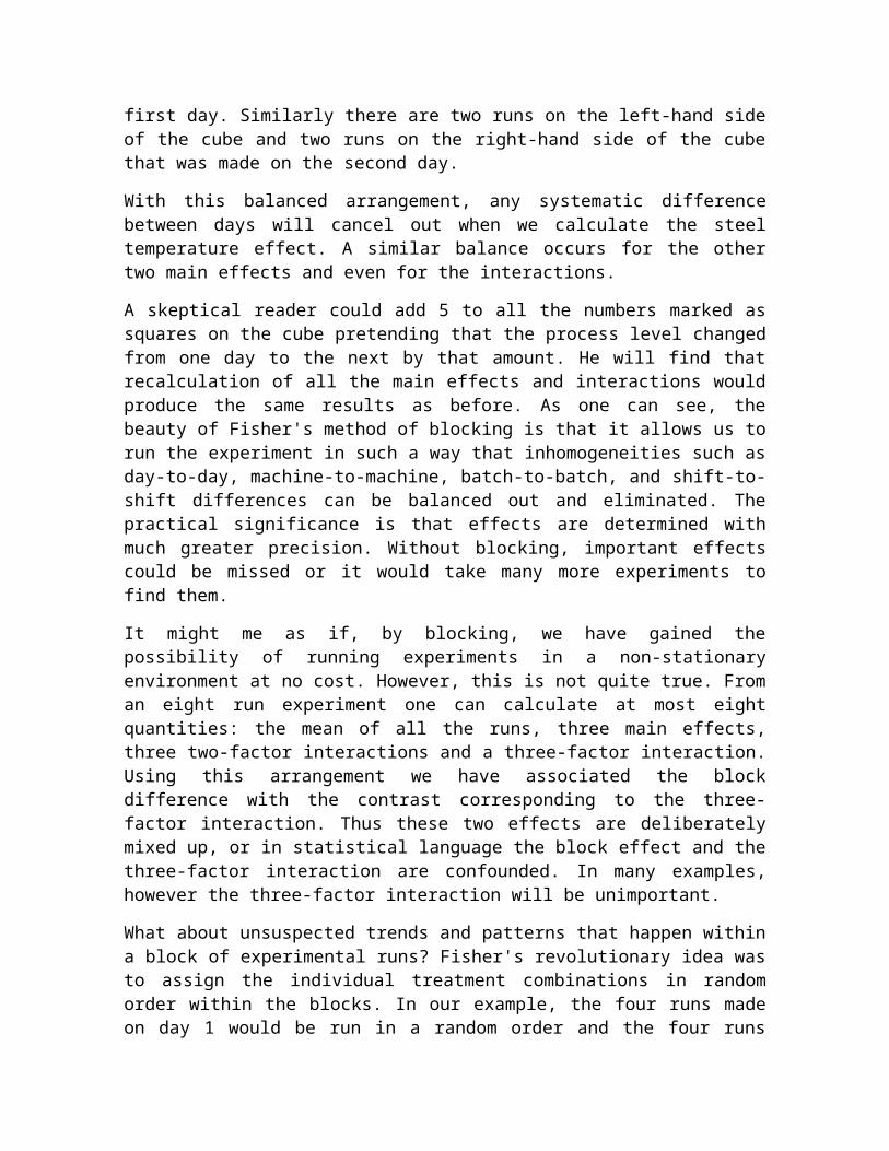
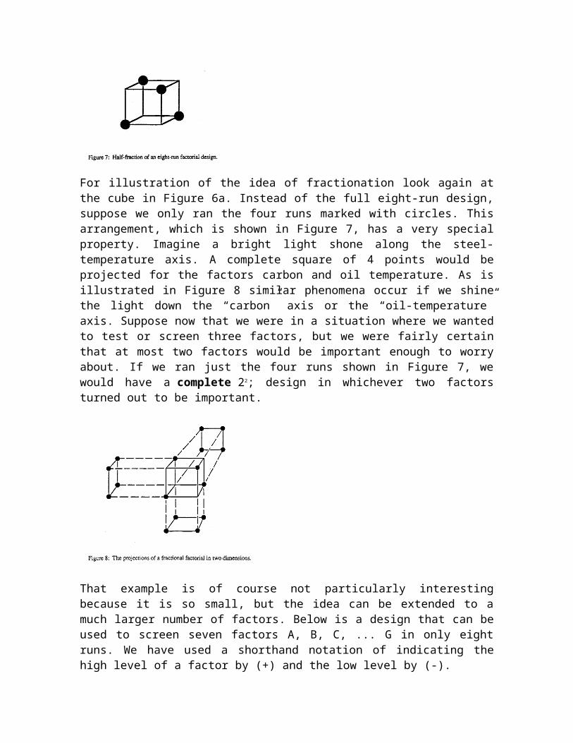
For illustration of the idea of fractionation look again at the cube in Figure 6a. Instead of the full eight-run design, suppose we only ran the four runs marked with circles. This arrangement, which is shown in Figure 7, has a very special property. Imagine a bright light shone along the steel-temperature axis. A complete square of 4 points would be projected for the factors carbon and oil temperature. As is illustrated in Figure 8 similar phenomena occur if we shine the light down the “carbon” axis or the “oil-temperature” axis. Suppose now that we were in a situation where we wanted to test or screen three factors, but we were fairly certain that at most two factors would be important enough to worry about. If we ran just the four runs shown in Figure 7, we would have a complete 22; design in whichever two factors turned out to be important.

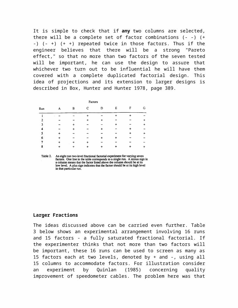
That example is of course not particularly interesting because it is so small, but the idea can be extended to a much larger number of factors. Below is a design that can be used to screen seven factors A, B, C, ... G in only eight runs. We have used a shorthand notation of indicating the high level of a factor by (+) and the low level by (-).

It is simple to check that if any two columns are selected, there will be a complete set of factor combinations (- -) (+ -) (- +) (+ +) repeated twice in those factors. Thus if the engineer believes that there will be a strong "Pareto effect," so that no more than two factors of the seven tested will be important, he can use the design to assure that whichever two turn out to be influential he will have them covered with a complete duplicated factorial design. This idea of projections and its extension to larger designs is described in Box, Hunter and Hunter 1978, page 389.

Larger Fractions

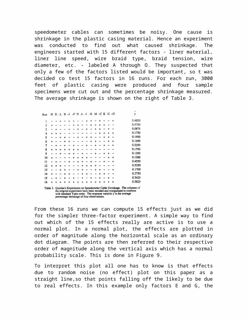
The ideas discussed above can be carried even further. Table 3 below shows an experimental arrangement involving 16 runs and 15 factors - a fully saturated fractional factorial. If the experimenter thinks that not more than two factors will be important, these 16 runs can be used to screen as many as 15 factors each at two levels, denoted by + and -, using all 15 columns to accommodate factors. For illustration consider an experiment by Quinlan (1985) concerning quality improvement of speedometer cables. The problem here was that speedometer cables can sometimes be noisy. One cause is shrinkage in the plastic casing material. Hence an experiment was conducted to find out what caused shrinkage. The engineers started with 15 different factors - liner material, liner line speed, wire braid type, braid tension, wire diameter, etc. - labeled A through O. They suspected that only a few of the factors listed would be important, so t was decided co test 15 factors in 16 runs. For each run, 3000 feet of plastic casing were produced and four sample specimens were cut out and the percentage shrinkage measured. The average shrinkage is shown on the right of Table 3.

From these 16 runs we can compute 15 effects just as we did for the simpler three-factor experiment. A simple way to find out which of the 15 effects really are active is to use a normal plot. In a normal plot, the effects are plotted in order of magnitude along the horizontal scale as an ordinary dot diagram. The points are then referred to their respective order of magnitude along the vertical axis which has a normal probability scale. This is done in Figure 9.

To interpret this plot all one has to know is that effects due to random noise (no effect) plot on this paper as a straight line,so that points falling off the likely to be due to real effects. In this example only factors E and G, the type of wire bud and the wire diameter, turn out to be important. So we have here a typical example of Juran's vital few (E and G) and trivial many (A,B,C,D,F,H,I,.J,K,L,M,N,O).

People often worry about the risk of using highly fractionated designs. The problem is that if main effects and interaction effects exist it will be impossible to tell from a highly fractionated experiment whether an observed effect is due to a main effect or an interaction.

The effects are mixed up or confounded with each other. Nevertheless, it is known from experience that fractional factorials often work very well. At least three different rationales for this have been advanced. One is that the experimenter can guess in advance which interaction effects are likely to be active and which are likely to be inert. We do not like this rationale. Ii seems to require rather curious logic. What this is saying is that while we cannot guess which main (or first-order) effects are important, we can guess which interactions (or second-order) effects are important. A second rationale is that by using transformations we can eliminate interaction effects. This is occasionally true but many interactions cannot be

transformed away. For example no transformation can eliminate the interaction effect taking place when two metals are combined to form an alloy.

The third rationale is based on the Pareto idea and the projective property of fractionals which we have discussed above. The most appropriate use of fractional designs, in our view, is for the purpose of screening when it is expected that only a few factors will be active. It may be necessary to combine them with follow-up experiments to resolve possible ambiguities. At later stages of experimentation when the important factors are known highly fractionated designs should not be used. For further discussion we refer to Box, Hunter and Hunter 1978, page 388.

Response Surface Methods

Much experimentation ultimately concerns the attainment of optimum condition-achieving, for example, a high mean or a low variance or both, of some quality characteristic. One method for solving optimum condition problems (Box and Wilson, 1951) prescribes proceeding through two phases. In phase I the experiment moves from relatively poor conditions to better ones guided by two-level fractional factorial designs. When near-optimal conditions have been found phase II is begun, involving a more detailed study of the optimum and its immediate surroundings. The study in phase II often reveals ridge systems much like the ridge of a mountain that can be exploited, for example, to achieve high quality at a lower cost. In phase II curvature and interactions become important. To estimate these quantities response surface designs were developed that are frequently assembled sequentially using two-level factorial or fractional factorial designs plus “star points” as illustrated in Figure 10 (see Box arid Wilson, 1951). These “composite” designs are not of the standard factorial type and for quantitative variables have advantages over three-level factorials and fractional factorials.

When the initial conditions for the experiments are rather poor, considerable progress can be made in phase I with simple two-level fractional factorial designs. The idea of sequential assembly of designs - developing the design as the need is shown can also be used with fractions. Thus (see, for example, Box, Hunter & Hunter, 1978) if, after running a fractional design, the results are ambiguous, a second fraction can be run selected so as to resolve these particular ambiguities.

Some of Taguchi's Contributions to Quality Engineering

The Japanese have been very successful in building quality into their products and processes upstream using fractional factorial designs and other orthogonal arrays. In particular, Professor Taguchi has emphasized the importance of using such experimental designs in

1) minimizing variation with mean on target,2) making products robust to environmental conditions,3) making products insensitive to component variation,4) life testing.

The first three categories are examples of what Taguchi calls parameter design. He has also promoted novel statistical methods for analyzing the data from such experiments using signal to noise ratios, accumulation analysis, minute analysis, and unusual applications of the analysis of variance. Unfortunately some of these methods of analysis are unnecessarily complicated and inefficient. To get the full benefit of his teaching, therefore, one must be somewhat selective. American industry can gain a competitive advantage by adding Taguchi's good quality ideas to those developed in the West and by combining them with more efficient statistical methods. We now discuss each one of the four important ideas listed above.

Minimizing Variation with mean on Target

The enemy of all mass production is variability. Any effort directed toward reducing variability will greatly simplify the processes, reduce scrap, and lower cost.

Figure 11 shows an experiment in which temperature, pressure and speed have been varied. Here, however, the output is not just a single datum point, but a whole set of observations. Therefore the cube plot has plots of the data in each corner. This diagram can be used to study the effect of the different factors on both the mean and the variance. In our example it can be seen, by simple inspection of the plots, that going from low temperature to high temperature has a tendency to move all the points up. Hence temperature can be used to move the mean on target. Again looking at the cube plot, it can be seen that going from the front face to the back face reduces variation. Thus speed affects variation.

This example is of course greatly simplified. In practice many more factors would be considered in fractional factorial or other orthogonal array designs. It illustrates the important idea that experiments can be used to bring the mean on target at the same time that the variance is minimized. In Taguchi's analysis of such experiments, however, a signal to noise ratio is used, which in this case is ten times the logarithm of the ratio of the mean and the standard deviation,

This signal to noise ratio approach seems unnecessarily complicated and too restrictive. An analysis in terms of SNT is essentially equivalent to first taking the logarithm of the raw data and then conducting the analysis in terms of the logarithm of the standard deviation. The assumption that would justify such an analysis is that a logarithmic transformation is needed to make the standard deviation independent of the mean. But sometimes to achieve this we need no transformation and at other times we need to use some other transformation, such as the square root or the reciprocal. Unless the logarithm is the right transformation the signal-to-noise ratio, SNT, will be inappropriate. For more on these technical issues we refer to Box (1987).

Often no exact measurements are available but the experimental results are of the ordered categorical type, for example, bad, fair, good, excellent. In the past (see, for example, Davies, 1947) it has been recommended chat scores such as 1,2,3,4 be assigned to such categories and the analysis proceed as if the numbers were actual measurements using standard statistical techniques. Taguchi has suggested a complicated method, for conducting such analyses which he calls Accumulation

Analysis. Extensive research (see Nair, 1986; Hamada and Wu, 1986; and Box and Jones, 1986) has shown that this method is inefficient and unnecessarily cumbersome and should not be recommended. The traditional method (see, for Example, Snedecor and Cochran, 1979) is not only simpler but also more efficient.

This is also true for the analysis of the speedometer cable shrinkage data already discussed. Here Quinlan follows Taguchi's recommendation and uses a signal-to-noise ratio and analysis of variance to analyze the experiment. This result a not only in a complicated analysis but leads to pronouncing factors important that are not. As we showed in Figure 9, normal probability paper provides a simple and efficient alternative. It was because analysis of variance for unreplicated experiments biased the results that Cuthbert Daniel, in 1959, proposed using the much simpler and intuitively pleasing normal probability plots that are particularly attractive to engineers. An additional useful tool is a Bayes' plot (see Box and Meyer, 1986).