CONTINGENCY DESIGNS FOR ATTITUDE

DETERMINATION OF TRMM N95- 27803

John L. Crassidis, Stephen F. Andrews, F. Landis Markley

Goddard Space Flight Center, Code 712

Greenbelt, MD 20771

Kong Ha

Orbital Sciences Corporation

Greenbelt, MD 20770

Abstract

In this paper, several attitude estimation designs are developed for the TropicalRainfall Measurement Mission (TRMM) spacecraft. A contingency attitudedet.erminafion mode is.required in the event of a primary sensor failure. The finalaeslgn utalizes a full sixth-order Kalman filter. However, due to initial software

concerns, the need to investigate simpler designs was required. The algorithmspresented in this paper can be utilized in place of a full Kalman filter, and requireless computational burden. These algorithms are based on filtered deterministic

approaches and simplified Kalman filter approaches. Comparative performances ofall designs are shown by simulating the TRMM spacecraft in mission mode.

Comparisons of the simulation results indicate that comparable accuracy withrespect to a full Kalman filter design is possible.

Introduction

The TRMM spacecraft is due to be launched in 1997 with a nominal mission lifetime of 42 months.

The main objectives of this mission include: (1) to obtain multi-year measurements of tropical andsubtropical rainfall, (2) to understand how interactions between the sea, air, and land masses producechanges in global rainfall and climate, and (3) to help improve the modeling of tropical rainfall processesand their influence on global circulation.

The spacecraft is three-axis stabilized in a near circular (350 km) orbit with an inclination of 35 °. The

nominal Earth-pointing mission mode requires a rotation once per orbit about the spacecraft's y-axis.The attitude determination hardware consists of an Earth Sensor Assembly (ESA), Digital Sun Sensors(DSS), Coarse Sun Sensors (CSS), a Three-Axis Magnetometer (TAM), and gyroscopic rate sensors.The attitude control hardware includes three Magnetic Torquer Bars (MTB) which are used to providemagnetic momentum unloading capability, and a Reaction Wheel Assembly (RWA) which consists of fourwheels in a pyramidal arrangement to maximize momentum storage capability along a preferred axis.

Primary attitude determination is accomplished using the ESA and gyroscopes. The DSS is also usedtwice each orbit in order to update the yaw position estimate during mission pointing. The allottedattitude knowledge accuracy is 0.18 ° per axis. Simulation studies indicate that the primary attitudedetermination system meets the knowledge requirements [1]. In the event of an ESA failure, acontingency mode is used to allow for the continuation of the scientific mission. Attitude determination

for the contingency mode is accomplished using the DSS, the TAM, and gyroscopes. The allottedattitude knowledge accuracy for the contingency mode is 0.7 ° per axis.

The algorithm chosen for the final contingency design incorporates a sixth-order Kalrnan filter [2].This filter estimates both attitude error angles and gyro drift trajectories. However, due to initialconcerns in software coding size and computations, the development of simpler and less software-

intensive algorithms is required. A number of algorithms is presented in this paper, including: anIsotropic Kalman Filter (IKF), a steady-state Angles-only Kalman Filter (AKF), an Enhanced TRIAD

419

https://ntrs.nasa.gov/search.jsp?R=19950021382 2018-09-16T07:28:24+00:00Z

Algorithm (ETA), and an Enhanced QUEST Algorithm (EQA). All of these algorithms utilize magneticfield measurements, digital sun sensor measurements (when available), and gym measurements. The IKFis a simplified Kalman filter in which an approximation is made where the rank deficient projection matrixis replaced by the identity matrix. This leads to attitude and gym bias covariances that are the same in alldirections in space. The AKF is a steady-state Kalman filter which estimates for angles only, with nogyro bias estimation. The ETA is essentially a first-order filter on TRIAD [3] determined attitudes.During solar eclipse, the ETA relies exclusively on model propagation using gyro measurements. Also,during sensor co-alignment the filter gain is automatically adjusted so that the filter relies more on thepropagated attitude. The EQA is similar to the ETA, but uses the QUEST [4] algorithm for attitudedetermination. This allows for weighting of individual attitude sensor _._urement sets.

The organization of this paper proceeds as follows. First, a summary of the spacecraft attitudekinematics is shown. Then, a brief review of the standard Kalman filter used for attitude estimation is

shown. Next, the equations and properties of the IKF, AKF, ETA, and EQA are presented. Then, these

algorithms are used to estimate the attitude of a simulated TRMM spacecraft. Finally, results are shownwhich compare each new algorithm to the full Kalman filter. A number of factors is considered,including: telemetry requirements, on-board requirements, coding size, and attitude accuracy.

Attitude Kinematics

In this section, a brief review of the kinematic and dynamic equations of motion for a three-axis

stabilized spacecraft is shown. The attitude is assumed to be represented by the quaternion vector,defined as

q =F ql3]

- Lq4.]

with

q-13 =- q2 =__sin(0/2)

q3

(1)

(2a)

(2b)

is the angle of rotation. The

q4 = COS(0 / 2)

where _ is a unit vector corresponding to the axis of rotation and 0

quatemTon kinematic equations of motion are derived by using the spacecraft's angular velocity (_),given by

(4a)

(4b)

_.coT :

where t)(t0) and _q_) are defined as

The 3 x3 dimensional matrices [,.ox]

ax_b. = _x]_b, with

. Fq413×3+[ q]3 ×]]

and [qi3 x] are referred to as cross product matrices since

420

I0a3aolC_a×]--"3 o i-a2 al

(5)

Since a three degree-of-freedom attitude system is represented by a four-dimensional vector, thequatemions cannot be independent. This condition leads to the following normalization constraint

qTq = qlT3q13 + q2 = 1

The measurement model is assumed to be of the form given by

BB=A(q)BI

(6)

(7)

where B_i is a 3 x 1 dimensional vector of some reference object (e.g., a vector to the sun or to a star, or

the Earth's magnetic field vector) in a reference coordinate system, __BB is a 3xl dimensional vector

defining the components of the corresponding reference vector measured in the spacecraft body frame,

and A(_q) is given by

a(_q) = (q42 -_qT3_ql3)13x 3 + 2 q_13_q_T3 - 2 q4[_ql 3 X] (8)

which is the 3 x 3 dimensional (orthogonal) attitude matrix.

Kalman Filter Review

In this section, a review of the basic principles of the Kalman filter applied to attitude estimation is

shown (see [2] for more details). The state error vector has seven components consisting of a four-

component error quaternion (Sq) and a three-vector gyro bias error a__b,given by

(9)

The error quaternion is defined as

8q=q®_ -1 (10)

where q is the true quaternion and 4 is the estimated quatemion. Also, the operator ® refers to

quaternion multiplication (see [3] for details). Since the incremental quaternion corresponds to a small

rotation, Equation (10) can be approximated by

which reduces the four-component error quaternion into a three-component (half-angle) representation.

The true angular velocity is assumed to be modeled by

02)

where to is the true angular velocity, cos is the gyro-determined angular velocity, and b_ is the gym drift

vector, which is modeled by

421

_b=rl 2

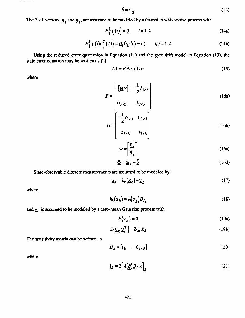
The 3 x 1 vectors, _-l and 112, are assumed to be modeled by a Gaussian white-noise process with

E{rli(t)}=O_Q i=1,2

(13)

(14a)

i,j = 1, 2 (14b)

Using the reduced error quaternion in Equation (11) and the gyro drift model in Equation (13), the

state error equation may be written as [2]

A__ = FAx+ Gw (15)

.i (16a)

(16b)

(16c)

wh_e

I I"-[0_ X] -_ 3×3

03x3 13x3

03 31L03×3 13×3j

w:r',,1- D2J

_=_o o -_ (16d)

State-observable discrete measurements are assumed to be modeled by

z_k =hk(Xk)+V k (17)

where

hk(Xk)=A(q_k)BI .

and v k is assumed to be modeled by a zero-mean Gaussian process with

(18)

E{V_k} =0 (19a)

E{v__t v__} = 8_ R t (19b)

Hk=[l k i 03x3] (20)

t, =2[A(_)_,×lk (21)

The sensitivity matrix can be written as

where

422

The extended Kalman filter equations for attitude estimation are summarized by

P=Fp+pTF+GQG T

ek(+)=[16×6-Kk Hk(_k(-))]Pk(-)

= +

= At;(+)

8q='(+)= (+)]

(22a)

(22b)

(22c)

(22d)

(22e)

(220

(22g)

Isotropic Kalman Filter

In this section, the equations for the IKF are shown. The state vector consists of an incrementalquaternion and gyro bias. The gyro propagation portion of the IKF is identical to the full Kalman filtershown in the previous section. However, the assumed measurement in the IKF is given by

_"= ff x fi (23)

where u_- is the measured unit vector from either the TAM or DSS in the body frame, and u_" is the

corresponding expected value, obtained by mapping the inertial reference to the body-fLxed coordinate

system using the estimated quatemion. Also, from Equation (23) __=0, since the cross product of a

vector with itself is zero. The sensitivity matrix of the measurement model in Equation (23) is determined

by using the attitude matrix of the angle error. This leads to

u- = A(_q.)__

where a__is an incremental error angle. Using the approximation

A(._.) = I3x3 = [___×]

leads to the following measurement model

(24)

(25)

z_-= (13x 3 -____T)0t (26)

Therefore, the sensitivity matrix, which contains partials with respect to the error state, is given by

H=[H u ! 03x3] (27)

where

Hu = I3x3 - -u-_T (28)

This matrix is the projection operator onto the space perpendicular to u_', which reflects the fact that an

observation of a unit vector contains no information about rotations around an axis specified by that

vector. Therefore, H,, has rank two. Also, if the measurement errors for each sensor are assumed equal

in all directions, then the measurement error covariance is given by

R = r H u (29)

423

where r is a scalar. Equation (29) indicates that there is no uncertainty in the length of the measuredvector. The IKF is derived by making an approximation of replacing the rank-two sensitivity matrix inEquation (28) by the rank-three identity matrix, which leads to

Hu = 13x3 (30a)

R = r/3x3 (30b)

This approximation leads to attitude and gyro bias covariances which are equal in all directions in space,or isotropic. Therefore, the covariance matrix has the form given by

p = ['Pa I3x3 Pc 13x31_Pc 13x3 Pbl3x3J (31)

where Po, Pc, and Pb are scalar quantities. Also, the state transition matrix is approximated by

_ = [13x3 -A/13x3][03x3 13x3 J (32)

where At is the sampling interval. Equation (32) ignores spacecraft rotation, which is irrelevant since theeovariance matrix in Equation (31) is isotropic. The covariance propagation equations are now given by

pak+l(_)=pak(+)_2Pck(+)At+Pbk(+)At2 +OvAt+._OuAt21 2 3

p_.+_(-)= p_ (+)- Pb.(+)_-2o __2"_

Pb..,(-)= Pb.(+)+o_t_

2 an d 2where o,, o v are the scalar covariances of the gyro-drift ramp

measurement noise, respectively. The Kalman gain matrix is given by

K =[ka13×3! kb13×3]r

where

ka- Pa_+l(-)

Pak+l (-) +r

kb = Pq+_(-)Pak+l (-) + r

Therefore, the Kalman covariance and state update equations are given by

Pak+l (+) = r k a

Pb_+,(+)= Pb_+l(-)-kbPc_+l(-)

[l ka(_ - __ ] qk+l (-)^ xu) @^qk+l(+) = z 1

-bk+z(+)=-bk+1(-)+kbC_×__)

noise, and

(33a)

(33b)

(33c)

the gyro-drift rate

(34)

(35a)

(35b)

(36a)

(36b)

(36c)

(37a)

(37b)

424

Since, Equations (37a) and (37b) depend on the cross product measurement (u_-x__), the updates to the

quaternions and biases are still perpendicular to u_"despite the approximation to the sensitivity matrix.

Steady-State Angles-only Kalman FilterIn this section, a simplified version of the full Kalman filter is shown. The AKF estimates only the

quaternion, and not the gyro drift. The covariance and state transition matrices are the upper 3 x 3 blocksof the corresponding matrices in a full Kalman filter. Therefore, covariance propagation is given by

Pk+l (-)=_ Pk (+) Cb+ w/3x3 (38)

where w is the assumed scalar level of the process noise. A full angles-only Kalman _ter rapidly

approaches steady-state using the covariance propagation in Equation (38). Therefore, a steady-state

covariance is used. An investigation of the eigenvalues of the covariance matrix shows that there is one

large eigenvalue (p,,,,_), and two nearly equal smaller eigenvalues (p,,_). Also, the eigenvector

corresponding to p,,,,= is found to always be within 2.5 degrees of the sun vector in the body. This

reflects the fact that the more accurate sun sensor cannot reduce attitude errors along the sun line, which

must be estimated using the less-accurate TAM. Therefore, the covariance matrix is given by

P = Peye 13×3 + Psun ssT (39)

where s_ is the sun vector in the body frame, and Pe_ and p,,,,, are constants. The minimum eigenvalue is

given by p,_, and the maximum eigenvalue is given by p,_ + p,_,,.

Sun Sensor Update

The sensitivity matrix and measurement covariance for the sun sensor are given by

Hs =[_x]

Rs = rs 13x3

(40a)

(40b)

where g_ is the estimated sun vector in the body frame, and r, is the scalar (isotropic) measurementcovariance. The Kalman gain for the sun sensor update requires the computation of

{HsP HT + Rs }-1= {poe[g - x]r + +R,}-'

1 113×3+Peyeg_S_T_ (41)

rs + Peye I rrsJ

Therefore, the Kalman gain matrix is given by

Ks = PHT{HsPH T +Rs} -1

1

rs + Peye

Peye

rs + Peye

f

{Peye /3x3 + Psun g_g_.T}[__xlT l/3x 3(42)

If the measurements are processed at a given time by accumulating an incremental error angle a.

initialized at zero, without re-computing the quaternion between updates, the state update becomes

425

e,e .3)rs + Peye

where s_- is the measured sun vector in the body frame.

TAM Update

The sensitivity matrix and measurement covariance for the TAM are given by

H t =[_x] (44a)

Rt = _ 13x3 (44b)

where __ is the estimated magnetic field vector in the body frame, and rt is the scalar (isotropic)

measurement covariance. The Kalman gain for the TAM update requires the computation of

{..e./+R,}-,={p_,[__×i__×1T+p,=f__×__)_×__)T+Rt} -I (45)

The inverseinEquation (45)iscomputable inclosedform, but iscomplicated. An approximation ismade

which assumes rtismuch largerthanboth p._ and Pun. Therefore,Equation (45)isre-writtenas

{.teH T +Rt}-l= l--13x3 (46)rt

The Kalman gain matrix is now given by

The state update is given by

K.=PHT{..P.T+R.}-'

=+{Peyel3x3+PsunS_S_T}{_x] T

^ A T N

}{.m×where _ is the measured TAM vector in the body frame.

__(_T_I3x3- tn thT)ct (-)}

(47)

(48)

Enhanced TRIAD and QUEST Algorithms

In this section, the ETA and EQA are developed. These algorithms are essentially based on an"alpha-type" [5] filter applied to deterministic methods. The TRIAD algorithm [3] involves theconstruction of two triads from a pair of orthonormal vectors, u_ and v, with basis vectors given by

l=u

uxvm- - --lu×Mn=Ixm

The basis vectors are constructed for both body measured vectors ua and ea, and for

reference vectors u I and e t . Two orthogonal 3 × 3 matrices are then constructed, given by

MB=[tB _B -_B]

MI=[1-1 m---I _I]

The attitude matrix maps the inertial reference to the body frame, and can be determined by

(49a)

(49b)

(49c)

the inertial

(50a)

(50b)

426

A = MBM T (51)

An accurate method for extracting the quatemions from the attitude matrix is given in [6].

The TRIAD method (as well as all deterministic) methods requires at least two sets of vectormeasurements to determine the attitude matrix. This method subsequently fails when only one set of

vector measurements (e.g., TAM data only) is available. Also, deterministic methods fail when vectorsare co-aligned (i.e., lu.v_]=l). These difficulties are overcome by combining the TRIAD determinedquatemions with a gyro-propagated model and a simple first-order filter. The ETA is given by

qp(+)= exp{1 D_g) At}__(-) (52a)

_0.(+) = (1-o_)qp (+)+c_ qtriad(+) (52b)

where qp is the propagated quaternion, q_."is the estimated quatemion, and q_,_,,, is the quatemion

extracted from the TRIAD determined attitude matrix. The scalar gain variable a is given by

= (1-[u x v_]e ) t0 (53)

where % is a constant gain. The filter gain in Equation (53) is automatically adjusted to accommodate

periods of vector co-alignment (i.e., as the vectors become co-aligned, the gain approaches 0). Also, a 0

is set to zero when only one measurement set is available.

The ETA is essentially a first-order "additive" Kalman filter. In general, this approach will notmaintain quaternion normalization [7]. To investigate how the ETA affects quaternion normalization,

Equation (52b) may be re-written as

__=qp®[Iq+lZ(q-pl®qtriad-lq) ] (54)

where lq is the identity quatemion. If the propagated quaternion is close to the TRIAD determined

quaternion, then Equation (54) can be approximated accurately byI-,i -I

(55)

where 80_ is the angle vector between qe and qt,_a" Therefore, since a 0 is very small, normalization is

maintained to within first-order. For numerical precision, the quaternions are explicitly normalized.

The EQA is similar to the ETA, but uses the QUEST [4] algorithm to determine attitude. The

QUEST algorithm minimizes the following cost function [8]

/i

(56)L(A)=l__ak__k-AVk[ 2k=l

where w is a set of unit vector observations in the body-frame, v is a set of unit observations with respect

to the inertial frame, and n is the total number of vector measurement sets. The constants a k serve to

weight individual sensor measurements. Shuster [4] has shown that the maximum-likelihood estimate of

the attitude is obtained with weights given by

1

ak o2 (57)

where o k is the standard-deviation of the measurement error process for each sensor.

427

TRMM Simulation and Results

In order to compare the algorithms developed in this paper, a simulation study is perfomw.d usingTRMM orbit parameters and performance criteria. The simulated spacecraft has a near circular orbit at350 km, and completes an orbit in approximately 90 minutes. The nominal mission mode requires arotation once per orbit (i.e., 236 deg/hr) about the spacecraft's y-axis while holding the remaining axisrotations near zero. The "true" magnetic field reference is modeled using a 10th order InternationalGeomagnetic Reference Field (IGRF) model. In order to simulate magnetic field modeling error, a 6thorder IGRF is used to develop "measurements." TAM sensor noise is modeled by a Gaussian white-noise process with a mean of zero and a standard deviation of 0.5 mG. The two DSS's each have a fieldof view of about 50°x 50 °. The body to sensor transformations for each sensor is given by

"-0.5736 0 -0.8192-

T1 _ 0.4096 0.866 -0.2868

0.7094 -0.5 -0.4967

"-0.5736 0 0.8192]/

-0.4096 0.866 -0.2868 /

-0.7094 -0.5 -0.4967J

T2 _

(58a)

(58b)

Each DSS views the sun when the sensor view is greater than the cosine of 50 °. The two DSS's combineto provide sun measurements for about 2/3 of a complete orbit. The DSS sensor noise is also modeled bya Gaussian white-noise process with a mean of zero and a standard deviation of 0.05 °. The gyro"measurements" are simulated using Equations (12) and (13), with a gyro noise standard deviation of0.062 deghtr, a ramp noise standard deviation of 0.235 deghtr/hr, and an initial drift of -0.1 deg/hr oneach axis.

A plot of the roll, pitch, and yaw attitude errors for a typical simulation run using the full Kalmanfilter is shown in Figure 1. A plot of the corresponding gyro-bias estimates is shown in Figure 2. FromFigure 1, the roll and yaw attitude errors show a strong dependence on orbit rate which is centered atzero, and a pitch error which is biased. This error bias may be due to non-Gaussian modeling errors inthe magnetic field "measurements." These nonlinearities cause an error in inertial space which is notzero-mean and is largely along the sun line. When these errors are mapped into the body frame,sinusoidal motions occur in roll and yaw which are 90 ° out of phase from each other. Also, a biasederror occurs in pitch which has the same magnitude as the sinusoidal motion, since the sun vector is 45 °off the pitch axis. This can be shown mathematically by redefining an inertial reference fixed on the orbitplane with the x-axis tangent to the orbit plane, the z-axis pointed nadir, and the y-axis completing thetriad. For a zero rotation, the inertial reference corresponds to the body frame. Therefore, from Figure 1a starting value for the inertial reference can be chosen such that the z-axis is zero, and the remaining axesequal in magnitude. The mapping to the body frame for a rotation about the y-axis is given by

cos(it) 0 Sino(it)] s cos(It)g=5 0 1 =__1_11 1 (59)

-sin(It) 0 cos(/a)J- 42 -sin(I.tl

is the direction of the sun vector,

(6O)

where Ix is the true anomaly, 8 is the magnitude of the error, and s

given by.

Clearly, a sinusoidal motion and constant bias is shown by Equation (59). This effect is also seen when

using a Kalrnan filter on other spacecraft (e.g., UARS and SAMPEX). However, the full Kalrnan filter is

able to estimate attitudes to within 0.1 °, and estimates the gyro-drift fairly accurately.

428

A plot of the attitude errors for a typical simulation run using the IKF is shown in Figure 3. There isno clear orbit rate dependence in roll and yaw for this algorithm, but all angle errors are now biased. Thismay be due to the fact that the IKF assumes that the attitude covariance is equal in all directions, so thatany biased errors are translated into all axes. The gyro-bias estimates (shown in Figure 4) are estimated

more accurately using the IKF, as compared to the full Kalman filter. However, comparing magnitudeattitude errors in Figure 3 to Figure 1 shows that attitude accuracy is no better than the full Kalman filter.

A plot of the attitude errors using the AKF is shown in Figure 5. The errors in roll and pitch arebiased, while the yaw error has a mean near zero. These errors are likely due to not correcting for gyrobias in the filter. This is further depicted in the attitude covariance matrix, which is an order of magnitudelarger than the full Kalman filter attitude covariance. However, attitude accuracy is still comparable tothe full Kalman filter (i.e., within 0.1 o).

A plot of the attitude errors using the ETA is shown in Figure 6. The peak errors seen predominatelyin the pitch and yaw errors are due to periods of sun un-observability. During these periods, the filtergain (shown in Figure 7) is set to zero, so that attitude is determined from gyro-propagation solely. Also,the gain clearly shows a sinusoidal motion. This motion compensates for measurement vector co-alignment. Attitude accuracy for this simple approach is within 0.15 °. Also, the EQA improves theattitude accuracy slightly, but not to any appreciable amount.

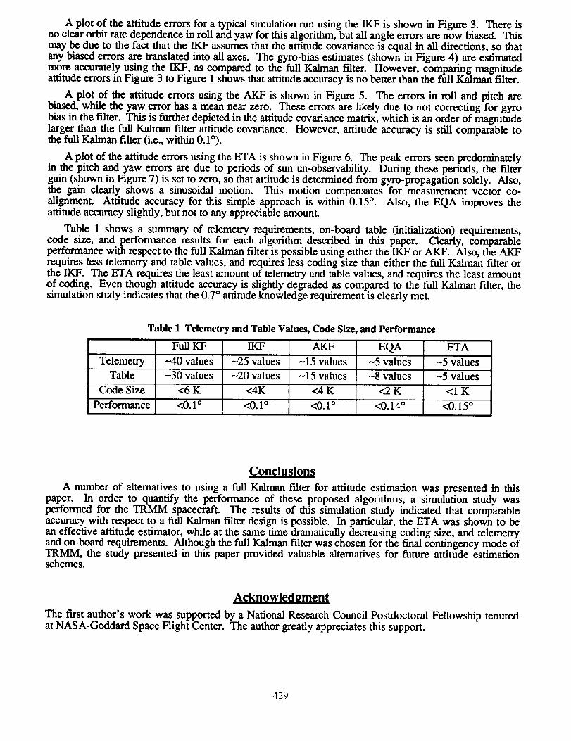
Table 1 shows a summary of telemetry requirements, on-board table (initialization) requirements,code size, and performance results for each algorithm described in this paper. Clearly, comparableperformance with respect to the full Kalman filter is possible using either the IKF or AKF. Also, the AKFrequires less telemetry and table values, and requires less coding size than either the full Kalman filter orthe IKF. The ETA requires the least amount of telemetry and table values, and requires the least amountof coding. Even though attitude accuracy is slightly degraded as compared to the full Kalman filter, thesimulation study indicates that the 0.7 ° attitude knowledge requirement is clearly met.

Table I Telemetry and Table Values, Code Size,

Full KF IKF

Telemetry -40 values -25 values

and Performance

AKF EQA ETA

-15 values -5 values -5 values

Table -30 values -20 values -15 values -8 values -5 values

Code Size <6 K <4K <4 K <2 K <1 K

<0.1 ° <0.14 ° <0.15 °Performance <0.1 o <0.1 o

Conclusions

A number of alternatives to using a full Kalman filter for attitude estimation was presented in thispaper. In order to quantify the performance of these proposed algorithms, a simulation study wasperformed for the TRMM spacecraft. The results of this simulation study indicated that comparableaccuracy with respect to a full Kalman filter design is possible. In particular, the ETA was shown to bean effective attitude estimator, while at the same time dramatically decreasing coding size, and telemetryand on-board requirements. Although the full Kalman filter was chosen for the final contingency mode ofTRMM, the study presented in this paper provided valuable alternatives for future attitude estimationschemes.

Acknowledgment

The first author's work was supported by a National Research Council Postdoctoral Fellowship tenuredat NASA-Goddard Space Flight Center. The author greatly appreciates this support.

429

References

[1] TRMM Attitude Control Subsystem Specifications, NASA-Goddard Space Flight Center (GSFC-TRMM-712-046).

[2] Lefferts, E.J., Marldey, F.L., and Shuster, M.D., "Kalman Filtering for Spacecraft AttitudeEstimation," Journal of Guidance, Control and Dynamics, Vol. 5, No. 5, Sept.-Oct. 1982, pp. 417-429.

[3] Wertz, J.S. (ed.), Spacecraft Attitude Determination and Control, D. Reidel Publishing Co.,Dordreeht, The Netherlands, 1984.

[4] Shuster, M.D., and Oh, S.D., "Three-Axis Attitude Determination from Vector Observations,"Journal of Guidance and Control, Vol. 4, No. 1, Jan.-Feb. 1981, pp. 70-77.

[5] Crassidis, J.L., Mook, D.J., and McGrath, J.M., "Automatic Carrier Landing System UtilizingAircraft Sensors," Journal of Guidance, Dynamics and Control, Vol. 16, No. 5, Sept.-Oct. 1993, pp.914-921.

[6] Sheppard, S.W., "Quatemion from Rotation Matrix," Journal of Guidance and Control, Vol. 1, No.3, May-June 1978, pp. 223-224.

[7] Bar-Itzhack, I.Y., and Deutschmann, J.K., "Extended Kalman Filter for Attitude Estimation of theEarth Radiation Budget Satellite," Proceedings of the AAS Astrodynamics Conference, Portland, OR,August 1990, AAS Paper #90-2964, pp. 786-796.

[8] Wahba, G., "A Least-Squares Estimate of Satellite Attitude," Problem 65-1, SIAM Review, Vol. 7,

No. 3, July 1965, pg. 409.

o.15r_

°.°751-I:oi_I.-oo; I0

Full Kalman Filter Attitude Errors

I ! [ I

I I I I

5 10 15 20 25

0.15

Xo.o750

.'I¢_¢k

00 5 10 15 20 25

.-. 0.15= , !

o.o R-A A-_0.151 ,_ i i

0 5 10 15 20 25Time (Hrs)

Figure I Kalman Filter Attitude Errors

430

Full Kalman Filter Gyro-Bias Estimates

! ! ! !

, i...............................z........,i...............ax

--0.20 1 2 3 4 5 6 7 8

,- 0.2_. ! ! ! , !............................i i i i-...............................................0 1 2 3 4 5 6 7 8

-_ °II_--__i ' ' ' ' ]

-0.2 i :,, i0 1 2 3 4 5 6 7 8

Time (Hrs)

Figure 2 Kalman Filter Gyro Bias Estimates

Isotropic Kalman Filter Attitude Errors

0"15l ' ' ' ' I.,-... . : : :

0.075[= ..................i...................:....................:.................:..................=_

_°-0.075=0 _iiiiiiiiii- ...................i....................?...................i..................

-0.150 5 10 15 20 25

I | I !

°:F i0 5 10 15 20 25

0.15, , , ,

_ o.o75 ..........i....................................i....................i..................0 _ii;iiii;ii

-0.15' I!

0 5 10 15 2O 25Time (Hrs)

Figure 3 Isotropic Kalman Filter Attitude Errors

431

Isotropic Kalman Filter Gyro-Bias Estimates

x /-0.2 i0 2 3 4 5 6 7 8

0.2, ' ' ' ' i i' ' i i-0.2 Iv i i , i i ; i

0 1 2 3 4 5 6 7 8

op_ ' ...................1 _" ........ _ : .... +

_0.21 i i i i0 1 2 3 4 5 6 7 B

Time (Hrs)

Figure 4 Isotropic Kalman Filter Gyro Bias Estimates

Angles-Only Kalman Filter Attitude Errors

0.15l_ _ _ v J ]

__o.o_°'°_"lIo ...................................._ i....................!:_....................................................................._........ . .........0 15 ........

0 5 10 15 20 25

°'151_ ': I

0 5 10 15 20 25

0.15

"-" 0.075o>- -0.075

-0.150 5 10 15 20

Time (Hrs)

Figure 5 Angles-only Kalman Filter Attitude Errors

i iiiiii ....}i....11i....iiiii '_........i....i....ii..........i....

25

432

Enhanced TRIAD Attitude Errors0.1, I !

i i0 5 10

; I15 20 25

_-. 0"2 i- , , , ,

-0.1 ' = i ,0 5 10 15 20 25

0.2 , , ! ,

0 5 10 15 20 25Time (Hrs)

Figure 6 Enhanced TRIAD Attitude Errors

t_t--

_o. 6<

X 10 -314

P12 ............_..................

10 ........... "...................

8 ..............................

4

Enhanced TRIAD Gain

I I I

!

-20 2 3 6 7 8

Figure 7 Enhanced TRIAD Filter Gain

433