continuous dynamic systems from transients - …dx01/bridge_material/biswas.pdf · discrete methods...

1

Vanderbilt University/MACS LabBridge Workshop – 03/01

TRANSCEND: Diagnosis ofContinuous Dynamic Systems

from TransientsGautam BiswasMACS Laboratory

Dept. of EECS Vanderbilt University

http://www.vuse.vanderbilt.edu/~biswas

Collaborators:Pieter Mosterman, Eric Manders, Joel Barnett,

Sriram Narasimhan, Philippus Feenstra, Liguo Yu

This project supported by: HP Labs (Agilent Labs), USA, PNC, Japan, the DARPA Software-enabled Control program (#

F33615-99-C-3611), and the NASA-IS program.


Model-Based Diagnosis of Dynamic Systems

• Values: Qualitative vs. Quantitative� qualitative models do not require numerical

parameter values but diagnosis is less precise� computational complexity of qualitative

methods may be less

• Temporal Behavior: Discrete vs. Continuous

� discrete methods may be easier to design but are less precise, coarser

� spurious results

FDI Models: examples

GDEState EstimationParameter Estimation

Quantitative

Sampath, et al.Lunze, et al.

Fault Signatures & TCGs(Mosterman and Biswas)

Qualitative

DiscreteContinuous

2


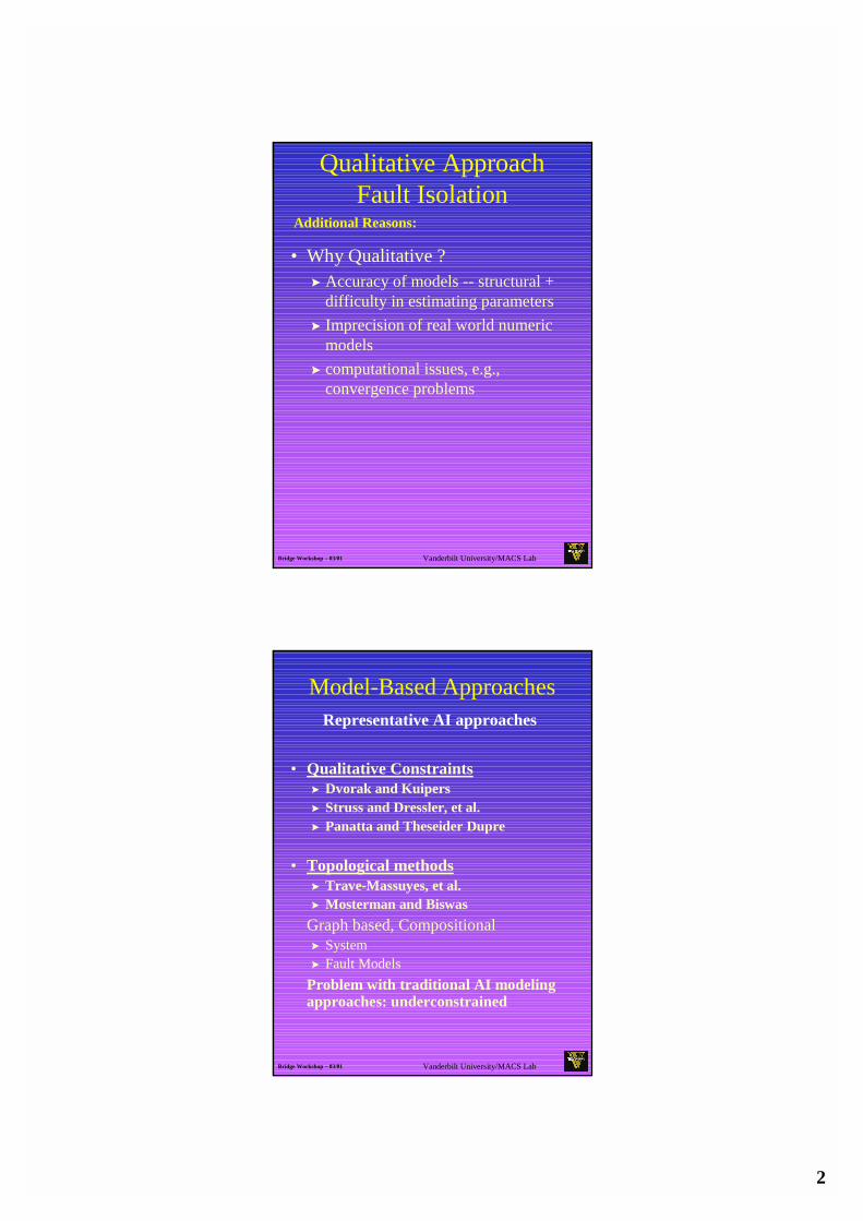
Qualitative ApproachFault Isolation

• Why Qualitative ?� Accuracy of models -- structural +

difficulty in estimating parameters � Imprecision of real world numeric

models� computational issues, e.g.,

convergence problems

Additional Reasons:


Model-Based Approaches

• Qualitative Constraints� Dvorak and Kuipers � Struss and Dressler, et al.� Panatta and Theseider Dupre

• Topological methods� Trave-Massuyes, et al.� Mosterman and Biswas

Graph based, Compositional� System� Fault Models

Problem with traditional AI modeling approaches: underconstrained

Representative AI approaches

3


Key Issues

• Dynamic, Continuous System• Abrupt Faults (not incipient or intermittent)

In theory, we are looking to characterize step response to abrupt change in a parameter value – called a transient.� Modeling Transients in Qualitative

Framework (Signatures) � Tracking dynamic effects of faults by

Progressive Monitoring

• Adequate Modeling Schemes(parameter to measurement relations)

•Work with Real Data�� Noisy, therefore, statistical techniques for change detection


Key Issues

• Parallels from control theory and systems dynamics -- Loop Analysis (e.g., Mason’s Gain rule) in control theory and Frequency Response Analysis

• Parallels from AI MBD approaches: reasoning in two steps: hypothesis generation and hypothesis refinement

• Differences from traditional FDI approaches – Qualitative Reasoning Framework + Local Analysis + Local to Global Propagation (i.e., consistency checking) over time

4


What are transients?Two Tank System --Response to Faults

Rb2

It seems one measurement is enough but not really….(especially if analysis is qualitative)& discontinuities not reliably detected...

f5:

Faults:Rb1, Rb2, R12

Discontinuity

Faults: C1, C2

Discontinuity


Diagnosis System ArchitectureThe TRANSCEND System

Observer scheme (Kalman Filter) uses numeric simulation model to track behavior – operates till fault occurs

Statistical techniques for symbol generation – activated from point of failure

Diagnosis model - qualitative temporal causal graph

5


Modeling for Diagnosis

• Dynamic, topological models• Need to describe both normal

and faulty system behavior.• Handle both qualitative and

quantitative information, if possible.� Qualitative Information -

magnitude deviations + higher order derivatives. (currently +, 0, -)

• Use Bond Graphs: Systematic modeling language, incorporates physical constraints in system models.


Bond Graph and Temporal Causal Graph

Two-tank System

e2

f1

f5 f8f3

e7

C1 C2

Rb1 R12 Rb2e2

f1

f3 f5 f8

e7

Second OrderSecond OrderSystemSystem

Bond GraphBond GraphTCGTCG

6


Two Tank SystemSteady State Model

e2

f1

f3 f5 f8

e7e2

f1

f5 f8f3

e7

C1 C2

Rb1 R12 Rb2


Diagnosis from Transients

Assumption: Model parameters in TCG correspond to system components.

Fault – model parameter that is deviated from its normal operating value

Abrupt Fault – parameter value change much faster than the measurement sampling rate (modeled as a step change).

Abrupt Faults cause transients in observed measurements.

Goal: Isolate fault as quickly as possible after occurrence of transient.

Two primary tasks:Two primary tasks:1. Reliable detection of transient2. Isolation of fault based on transient

characteristics

7


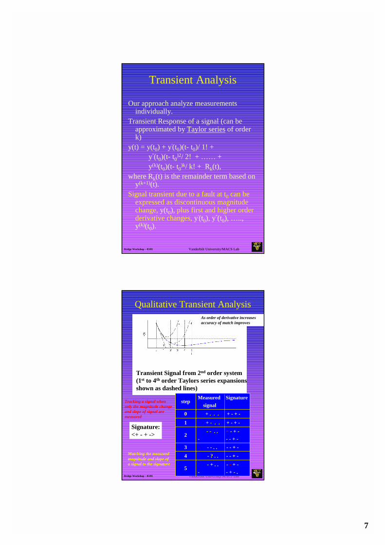
Transient Analysis

Our approach analyze measurements individually.

Transient Response of a signal (can be approximated by Taylor series of order k)

y(t) = y(t0) + y'(t0)(t- t0)/ 1! + y''(t0)(t- t0)2/ 2! + …… +y(k)(t0)(t- t0)k/ k! + Rk(t),

where Rk(t) is the remainder term based on y(k+1)(t).

Signal transient due to a fault at t0 can be expressed as discontinuous magnitude change, y(t0), plus first and higher order derivative changes, y'(t0), y''(t0), ….., y(k)(t0).


Qualitative Transient Analysis

Transient Signal from 2nd order system(1st to 4th order Taylors series expansionsshown as dashed lines)

- + . . - -- + -- - + - .

5

- ? . . - - + -4- - . . - - + -3

- - . . ++ - + -- - - + -

2

+ - . . + - + -1

+ . . . + - + -0

Measured Signature signal

step

As order of derivative increases accuracy of match improves

Tracking a signal whenonly the magnitude changeand slope of signal aremeasured

Signature:<+ <+ -- + + -->>

Matching the measured magnitude and slope of a signal to the signature

8


Fault SignatureSignal feature vector in response to a fault

expressed as a sequence of qualitative derivative values at the point of failure.

Qualitative Fault Signature of order k: fault signature that includes derivatives up to order k.

Assumption – The sampling rate of the measured signals is set to be fast enough so that no qualitative change in the transient dynamics is missed.

Fault Isolation Task:1. Detect transients and hypothesize

possible faults2. Generate fault signatures for all

measurements based on hypothesized faults.

3. Fault Isolation by Progressive Monitoring.


The Diagnosis Process

1. Generate Fault Hypotheses -Backward Propagation

2. Predict Behaviors - Forward PropagationResult: Individual Fault Signatures

3. Prediction to the limit -Steady state analysis

4. Monitoring - compare signatures to observationsSchemes: Progressive Monitoring & Discontinuity Detection

9


Generate Fault Hypotheses

-C2 -R12+Rb2 +Rb1-C1

+

+

-

e4

f3-e6

-e8+f6

+

+

++

-

-

-

--

+e7 C2f8

e7R12

Rb2f7

f5e2e5

e7

+

-

-

-

+

-

-C1

Rb1

f4e2

f2

e3

f5

Possible Faults:

Rb2e2

f1

f5 f8f3

e7

C1 C2

Rb1 R12 Rb2

f1

f3 f5 f8

e2 e7


Prediction by Forward PropagationSignatures

Qualitative Signature: magnitude + first and higher order derivative changes expressed as +,0,- values.

How to generate signatures from TCG ?Temporal links imply integrating edges, affects

derivative of variable on the effect sideStart with 0-order changesEvery integrating edge increases order by one

Rb2+ 2nd Order signature of e7: < 0,+,- >

10


Progressive Monitoringtrack system behavior after failure

• System Behavior Convolutes the Predicted Transient at Time of Failure� dynamically change the signature

Justified by Taylor’s series

Only Model Observable Behavior!

signature1k

0 0 + -

1 + + -

2 + + -

3 + + -

match!

signature2k

0 + - +

no match!

measurek

0 0

1 +

2 +

3 + +

4 + 0

5 + -

6 + - -

1 2 3 54 t6


Monitoring for Dynamic Systems

When to suspend transient analysis.• (a) Compensatory Response• (b) Inverse Response: slope reverses• (c) Reverse Response: (overshoot)

slope and magnitude change sign

(a)

(b)

(c)

Temporal Behavior: Signal Transients

11


Simulated Two Tank System• Using Progressive Monitoring• Rb2

+, e7, f3 measured

For each signal measuring magnitude change,slope, and eventual steady state value

R12 Rb2e2

f1

f5 f8f3

e7

C1 C2

Rb1

f1

f3 f5 f8

e2 e7


(1) ACTUAL => f3: 0 . . . e7: 1 . . . ================C2- => f3: 0 1 -1 e7: 1 -1 1 Rb2+ => f3: 0 0 1 e7: 0 1 -1 R12- => f3: 0 -1 1 e7: 0 1 -1 C1- => f3: 1 -1 1 e7: 0 1 -1 Rb1+ => f3: -1 1 -1 e7: 0 0 1

(2) ACTUAL => f3: 1 1 . . e7: 1 -1 . 1 ============= ===C2- => f3: 0 1 -1 e7: 1 -1 1

(4) ACTUAL => f3: 1 0 . . (-> S) e7: 1 -1 . 1 ======== ========C2 - => f3: 0 1 -1 e7: 1 -1 1

(7) ACTUAL => f3: 1 0 . . (-> S) e7: 1 0 . 1 (-> S)======== ========C2 - => f3: 0 1 -1 e7: 1 -1 1

e7

f3

2

2

4

4

7

7

tf

tf

Simulated Two Tank System

• Using Discontinuity Detection• C2-, f3 and e7 measured

For each signal, measuring - magnitude change,slope, steady state value, initial change discontinuous

e2

f1

f5 f8f3

e7

C1 C2

Rb1

f1

f3 f5 f8

e2 e7R12 Rb2

12


Three Tank Results

Measured Variables are p1, p2 and f12Faults Introduced Faults Identified Steps Taken

C1+ C1+ 6C2+ C2+ 5C3+ C3+ 8

R12+ R12+ 10R23+ R23+, Rb+ 14Rb+ R23+, Rb+ 21

f5 e7==

e3

e5

1dt dt

-1 -1= =

-1 =

=1 = 1e2

e1

e6e4 f4

f3 f7

f6F1 f21

R121

C11C2 f9 e11

e9

1dt

-1

=

-1

= 1 e10e8 f8 f11f101

R231Rb

=

1C3


Secondary Sodium Cooling Loop

(Note: 6th order system)

Bond Graph Model

super heaterevaporator

mainmotor

sodiumoverflowtank

secondarysodium

pump

intermediateheat exchanger

sodium flow stopping valve(normally opened)

sodium flowstopping valve(normally opened)

feedwaterloop

feedwaterloop

CE V

CSH

GY

R4

R5

R3

COFC

R2

e33

R1

Vin

II H X

e19e22

f11

e14

13


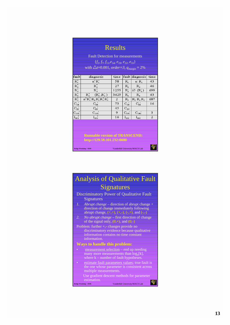
ResultsFault Detection for measurements

{f2, f7, f11,e14, e19, e22, e33}with ��t=0.001, order=3, qmargin = 2%

Runnable version of TRANSCEND: http://129.59.101.232:8080


Analysis of Qualitative Fault Signatures

Discriminatory Power of Qualitative Fault Signatures

1. Abrupt change – direction of abrupt change + direction of change immediately following abrupt change, (+,+), (+,-), (-,+), and (-,-)

2. No abrupt change – first direction of change of the signal only, (0,+), and (0,-)

Problem: further +,- changes provide no discriminatory evidence because qualitative information contains no time constant information.

Ways to handle this problem:• measurement selection – end up needing

many more measurements than log4[k], where k – number of fault hypotheses.

• estimate fault parameters values; true fault is the one whose parameter is consistent across multiple measurements. Use gradient descent methods for parameter estimation.

14


Parameter Estimation

GenerateParameterized

State Equation Model

Parameter Estimation

(System ID methods)Decision

Procedurefh

fh’

• Initiate a fault observer for every singlefault hypothesis, fh -- multiple observers

• Each observer has only one unknownparameter that is unknown -- simplifiedsystem ID methods can be employed

• For true fault, parameter estimate improvesas more measurement samples obtained --should converge to true value

• For other fault hypotheses, parameter estimate should diverge


Extended Parameter Estimation

• Substitute numeric values for all parameter values except faulty parameter.

•Estimate parameter value using standard least square estimation techniques.

• Predict values for all measurements and check for divergence

11

3

2

1

1111111111

5242524232223222

3121312111

3

2

1

00

1

111110

11111111

011111

.

.

.

fC

hhh

RCRCRCRCRC

RCRCRCRCRCRCRCRC

RCRCRCRCRC

h

h

h

+�

��

�

�

−−−+

+−−−−+

+−−−

=

��

��

�

�

15


Parameter Estimation example

Convergence of predictionestimates for measurementsto 0 for true fault

Divergence of error in estimates for measurements for other hypothesized fault


Conclusions• Developed a comprehensive methodology

for diagnosis based on transient analysis� FDI-based models to capture continuous

dynamics� Derived topological model (TCG) for localized

analysis of faults – dynamics captured as fault signatures

� Progressive Monitoring to match signatures to observations

• Dealing with real signals but processing them qualitatively – required signal to symbol transformation techniques (based on time-frequency analysis)

• Limitations of qualitative reasoning led to combined approach. Reduced set of fault hypotheses spawned fault observers for fault parameter estimation

• Now extended to diagnosis of hybrid systems

16


The TRANSCEND SystemReferences

• P.J. Mosterman and G. Biswas, “Monitoring, Prediction, and fault Isolation in Dynamic Physical Systems, Proc. AAAI-97, pp. 100-105, Providence, RI, July 1997.

• P.J. Mosterman and G. Biswas, “Diagnosis of Continuous Valued Systems in Transient Operating regions,” IEEE Trans. On Systems, Man, and Cybernetics, vol. 29A, no. 6, pp 554-565, Nov. 1999.

• E.J. Manders, et al., “A combined Qualitative-Quantit-• ative for efficient Fault Isolation in Complex Dynamic

Systems, Safeprocess, pp. 1074-1079, 2000.

• E.J. Manders, P.J. Mosterman, and G. Biswas, “Signal to Symbol Transformation for Robust Diagnosis in TRANSCEND,” Tenth Intl. Workshop on Principles of Diagnosis, Loch Awe, Scotland, pp. 155-165, June 1999.

• S. McIlraith, G. Biswas, D. Clancy, and V. Gupta, “Towards Diagnosing Hybrid Systems,” Tenth Intl. Workshop on Principles of Diagnosis, Loch Awe, Scotland, pp. 193-203, June 1999.

• Narasimhan, et al., Safeprocess 2000• Narasimhan and Biswas, DX-01.

Fundamental Approach

Limitations of Qual. Reas./Combined Approach

Signal Analysis – Signal to Symbol Transformation

Hybrid Diagnosis


Wavelet Transform• DWT applied to step function with

Gaussian noise.

• Nine level decomposition

Threshold at level 4 Threshold at level 5

σσσσ = 0.2 σσσσ = 0.4

17


Feature Extraction from Transients

• Signal Magnitude (+,-): simple filter that avoids fluctuations around zero crossings

• Slope estimation:� first order difference operator� finite impulse response (FIR) filter FIR

coefficients: h(n) = (N-1)/2 - n ; n=0,….,N-1

k=0

N-1Differentiator: y(n) = S h(k)x(n-k)

continuous dynamic systems from transients - …dx01/bridge_material/biswas.pdf · discrete methods...

Documents