contribution of fertility model and parameterization …...mortality assumptions as up to 0.02...

1

WP 8.1

16 October 2013

UNITED NATIONS STATISTICAL COMMISSION

and ECONOMIC COMMISSION FOR EUROPE

STATISTICAL OFFICE OF THE

EUROPEAN UNION (EUROSTAT)

Joint Eurostat/UNECE Work Session on Demographic Projections

organised in cooperation with Istat

(29-31 October 2013, Rome, Italy)

Item 8 – Assumptions on future fertility

Contribution of fertility model and parameterization to population

projection errors

Dalkhat M. Ediev, Wittgenstein Centre (IIASA, VID/ÖAW, WU)

Literature offers a wide range of fertility models of different type and complexity that may be

used in population projections. Yet, systematic studies are not available that would quantify,

how important are the model complexity and right choices of the model parameters for the

projection accuracy. This work provides the needed comparative study of contributions to the

population prediction accuracy of model form and of the accuracy of the three main fertility

indicators (the total fertility, mean and standard deviation of age at birth, respectively: the

TFR, MAB, SDAB). We apply to the empirical female populations set of (about thirty)

fertility models and study the deviations of the imputed numbers of births from the empirical

ones. Our set of fertility models includes variants of the direct transformation of the empirical

schedule; Schmertmann’s Quadratic Spline model; the Gamma model; the Beta model; the

Rectangular model; the Ryderian pentapartite model; and combinations of those models with

abridging into 5- and 10-year age groups and regression models. Some other models (e.g., the

Brass model) have also been tried but not reported here because, being computationally more

demanding, they showed worse performance than other models of a similar structure. Our

data come from the Human Fertility Database, Recent Demographic Developments’ reports

by the Council of Europe, Human Fertility Collection, Eurostat’s and UN Population

2

Division’s estimates and cover (after merging and cleaning) 5887 country-years of

observation. We came to a set of findings, often counter-intuitive, that may be instructive in

population projections. Most notably, we find high importance of accuracy of the TFR and

MAB in population projections. The role is limited, yet considerable, of estimates of the

SDAB and of the choice of the fertility model form. We suggest to avoid abridging fertility

rates, using analytical fertility models, modeling age-specific rates directly, or working with

disaggregated (e.g., by parity) rates. Our recommended approach would be, first, to model

MAB and SDAB and, second, to transform, however estimated beforehand, age-specific

fertility rates to fit exactly the projected MAB and SDAB. Making use of our findings already

reduces the mean squared prediction errors by half as compared to existing practices.

1. Introduction

Fertility models and assumptions are the main drivers of population forecast errors in short-

and long-time horizon. In the US context, contribution to population mean squared forecast

errors of accuracy of initial population estimates was estimated as 0.3 percent, that of

mortality assumptions as up to 0.02 percent, of migration as up to 0.1 percent, but

considerably more, 5-10 percent, was the estimated contribution of fertility estimates (Alho

1992). The latter estimate is roughly comparable to the mean squared annual change of TFR

of about 4 percent in the Human Fertility Database (2013). The leading role of fertility

assumptions in determining population forecast accuracy justifies detailed analysis of various

ingredients of fertility assumptions, such as models used to describe its time and age

variation. Meanwhile, the period total fertility rate (TFR) is the prime, if not the only, fertility

indicator commonly used in producing the population projection scenarios (e.g., Eurostat

2011; U.S. Census Bureau. 2012; United Nations 2013). The age distribution of fertility,

usually, remains behind the scene and is rarely reported in the projection literature. The most

recent UN World Population Prospects 2012 (United Nations 2013), the most advanced, well-

3

done, and authoritative international projections as of today, offer great methodological

advances and many details in modeling the Total Fertility but barely anything about modeling

the age variation of fertility. Such a situation is quite typical for the population projection

literature at large. Indeed, a common practical method is simply to scale up or down the

baseline age pattern of fertility according the projected TFR levels.

Such simplifications may work well for low-mortality, no-migration stationary

populations where population sizes of fertile age groups are equal and any age profile of

fertility rates produces the same number of births as long as the TFR is fixed. In a population

with n persons in each of the single-year fertile age groups, there will be TFR*n births each

year. More realistically, population sizes of fertile age groups vary substantially because of

time-varying sizes of birth cohorts and effects of migration and mortality. Such irregular age

profiles may produce differing numbers of births and projected populations when combined

with fertility curves of the same total fertility but differing age patterns.

Another set of practical questions refers to how to describe (and, hence, to model) the

age pattern of fertility rates. A concise description of it involves, usually, the mean and the

standard deviation of age at childbearing (MAB and SDAB, respectively) – indicators found

important in fertility and dynamic population models. More complicated fertility models

involving more than three parameters have also been proposed in the literature and shown to

better fit the empirical fertility schedules. A common sense and some advanced approaches in

the projection literature assume superiority of more detailed fertility descriptions over less

nuanced ones. This assumption, however, has never been tested systematically and, it appears

in our study, seems not to be valid.

Our work aims to improve understanding of the role of different ingredients of fertility

projections through a comparative analysis of importance of model choice and of the three

main fertility parameters (TFR, MAB, and SDAB) in projecting the number of births. Model-

wise, we consider about thirty different fertility models of different sophistication levels.

4

Using empirical population compositions and fertility rates, we study deviations of the

predicted number of births from the empirical number under alternative models of the age

pattern of fertility rates and for different approximations of the fertility parameters.

2. Data and methods

Appreciating the sensitivity of the projected number of births to accuracy of the TFR is

straightforward. A one percent error in the TFR, the age pattern of fertility being intact, would

result in a similar one percent error in the projected number of births. Sensitivity to the

projection errors in the age pattern of fertility is, however, harder to study because of

interaction of these errors with the age composition of the population to which the fertility

pattern is applied. In a population with a ‘flat’ age pattern at fertile ages the accuracy of the

fertility pattern (given the TFR is fixed) hardly matters. On the contrary, in projecting a

population with strongly skewed age composition applying the same TFR to younger or older

cohorts at childbearing ages may produce different numbers of births.

Some insights, even if under unrealistic assumptions, may be gained through

analytical derivations. Ediev (2013) shows, in particular, that the relative prediction error of

the number of births in a stable population may be approximated as 2rr , where r

is the population growth rate, is the bias in the MAB, is the bias in the SDAB and is

the SDAB. Given typical SDAB around 5 years and population growth of fractions or, at

most, of few percent per year, it is clear that the effect of the bias in MAB is dominating over

the effect of bias in SDAB. More so, if we take into account that biases in MAB are, usually,

higher in absolute value than biases in SDAB. Despite important insights from the above

relation, its practical value is rather limited. That is because populations are seldom stable

and, in particular, the estimate above of the contribution of the bias in SDAB into births

prediction error is far too small for a real population. Under stylized, yet realistic, assumptions

(r=0.5%, SDAB=6 years, =1.6 years, and =0.5 years) the formal relation suggests 0.8%

5

errors originating from the biases in MAB and only 0.008% errors due to biases in SDAB –

both too low, as compared to our simulations-based estimates of 1.4% and 0.37% errors,

respectively (see further down in the paper).

A more practical and realistic estimates of contributors to births prediction errors may

be done through numerical simulation using data on actual populations. To this end, we use

five detailed international population and fertility databases (Human Fertility Database 2013;

Recent Demographic Developments 2005; human Fertility Collection 2013; Eurostat database

2013; and UN (2013) World Population Prospects 2012: HFD, RDD, HFC, WPP, and IDB,

respectively, in the following text). Based on empirical data, we simulate percentage errors of

the predicted numbers of births assuming variety of typical model simplifications about the

age pattern of fertility rates. The five databases contain estimates, respectively, for 27, 43, 73,

59, and 236 populations with different calendar coverage and total 1634, 1757, 3774, 3127,

and 2832 country-years covered (5887 country-years after merging the datasets and cleaning

the repetitive entries). The pooling was done with following priority of the databases:

HFD>RDD>HFC>EUSt>WPP. (If the same database, in that case HFC, had different

estimates for the same population in the same year, we averaged those different estimates.)

These datasets cover practically the entire range of typical fertility and population structures,

both modern and historical.

To each empirical female population we apply a model age profile of fertility rates,

with TFR set at the empirical level, and see how far the imputed number of births deviates

from the empirical number. We tried number of models of age-specific fertility (about 30

individual models and combinations) and number of scenarios for the MAB and SDAB (seven

scenarios for each). As noted above, we do not vary the TFR, because contribution of bias in

TFR to births prediction error is straightforward and needs no simulations to assess: one

percent error in TFR produces one percent error in the number of births.

6

More specifically, we tried the following models for the age-specific fertility: direct

transformation of the empirical schedule; Schmertmann’s Quadratic-Spline model; the

Gamma model; the Beta model; abridging the fertility rates into 5- and 10-year age groups;

regressions of fertility rates over TFR and MAB based on a selected dataset; the Rectangular

model; and the Ryderian pentapartite model. Some of the models are described next.

In our simplest model, we transform the empirical pattern of age-specific fertility rates

directly, according to the assumed model values of the MAB and SDAB:

k

MABxMABf

kxf ee1

, (1)

here xf is the fertility rate at age x, superscript ‘e’ denotes the empirical schedule, and

eSDAB

SDABk . Multiplier ‘

k

1’ before the empirical schedule assures identical TFR’s in the

empirical and transformed schedules; in calculations, we use discrete approximation to (1)

and adjust the multiplier to match exactly the assumed TFR. Occasionally, the transformed

rates may turn non-plausible when positive at ages beyond the fertile age limits. We overcome

this problem by applying (1) only in the age range 12-54 and setting fertility rates zero outside

that range.

In the next model, we approximate the baseline age pattern in (1) through a linear

regression of age-specific fertility rates on the TFR and MAB:

MABcTFRbaF xxxx , (2)

where the regression coefficients are estimated either over the entire database or based on data

for a given country only. Once the baseline (2) is set, we apply transformation (1) to fit

exactly to the assumed values for the TFR, MAB, and SDAB.

Description of Schmertmann’s Quadratic Spline model, of Gamma and Beta models

may be found in Ediev (2013) and in the original literature (Schmertmann 2003; Hoem et al.

1981). We reduce the Gamma and Beta models into two-parametric variants, by setting Alfa4

7

to zero in the Gamma model and Alfa to 12 and Beta to 55 in the Beta model. Also note that,

unlike in some other works, we fit these models to assumed values for the MAB and SDAB,

and not to the whole age pattern of fertility rates. For Gamma and Beta models, that is

possible using analytical relations. QS model requires optimization.

The Rectangular, as well as the following Ryder’s, model serves as an extreme

example of model simplification. It is based on assuming age-independent fertility in an age

range bax , and zero fertility outside the range:

,,,0

,,,

bax

baxab

TFR

xf (3)

SDABMABa 3 and SDABMABb 3 assure match to assumed MAB and SDAB.

Ryder’s (1989) ‘tetrapartite’ model assumes fertility rates are all set zero except at four

equally-distanced ages. Our calculations show that better results are produced by the

pentapartite model (used in this work) where fertility rates are all zero except at five equally

spaced ages 17.5 to 37.5. Hence, in our pentapartite model, fertility rates at ages 17.5, 22.5,

27.5, 32.5, and 37.5 are selected in order to fit to the assumed values for TFR, MAB, SDAB,

and, to improve the robustness of the procedure, to minimize the sum of squares of the rates.

Our summary indicator of prediction accuracy is the mean squared relative error

(MSRE) of the predicted number of births:

N

i i

ii

B

BB

NMSRE

1

2ˆ1

, (4)

where iB and iB̂ are the observed and predicted numbers of births obtained by applying the

exact and the approximate fertility schedules, respectively, to population ‘i’; N is the total

number of populations in the database. This indicator in convenient in possibility to compare

it, one-to-one, to the errors induced by the biases in the TFR (a one per cent bias in TFR

produces a similar error in the projected number births). In addition to the summary MSRE’s,

8

we also consider full distributions of the prediction errors because the distributions show

considerable excess kurtoses and prolonged tiles at both ends of the distribution.

Models’ parameterization is based on a combination of assumptions about MAB and

SDAB (the TFR is always set at its empirical level): the exact empirical value; the average

over all populations of the DataBase; country-specific average; regression-based

approximation with the TFR and TFR^2 (and, for the SDAB, the MAB) used as the predictors

(regressions are fit over the whole DB); country-specific linear regressions with the TFR used

as the predictor; country-specific linear regressions with the TFR and t (time) used as the

predictors.

3. Results and implications

Selected MSRE’s by database are presented in Table 1. The most simplistic–and atypical for

projection practices–approximations aside, inability to project exactly the MAB is the most

important contributor to prediction errors. Among the MAB approximations tested in the

paper, the most efficient happened to be the one based on a country-specific regression on

TFR and time. That approximation contributes more than one percentage point to the

prediction errors, a value comparable to TFR’s contribution (about 4 per cent as mentioned in

the introduction) and exceeding contributions of other components, such as model-choice- or

SDAB-related errors. In fact, quite against intuition, the cost of poor approximation of MAB

is comparable (for the best approximation) or even exceeds (for the less efficient

approximations) errors due to abridging into 10-year age groups or even assuming a

rectangular shape of the fertility age pattern. The Table also illustrates that the common

practices of abridging the fertility rates into five-year age groups and using analytical fertility

models also have considerable contributions to the prediction errors and better be avoided. It

may also be noticed here that the Beta model, even if comparable to the Gamma model in

terms of prediction errors, does so only after adjusting the model fertility rates in order to

assure exact match to MAB and SDAB.

9

Another important message from Table 1 is that the simulation results are rather

similar for all five databases. We, therefore, present more details of the simulations based on

the pooled dataset of 5887 population-years of observation we kept after merging the five

databases and cleaning the data for repetitions (somewhat different set of estimates based on

HFD data only may also be found in Ediev 2013).

Table 2 summarizes MSRE’s in simulations based on the merged database. When both

the MAB and SDAB are set at their actual values (the first row with simulation results), the

MSRE’s correspond to errors due to model structure. Not surprisingly, the Rectangular and

Pentapartite models show rather poor performance. More of a surprise is a similar poor

prediction efficiency of four other models: abridging into 10-year age groups; Beta model

with parameters obtained from the common formal relations; and obtaining age-specific rates

from regressions on TFR+MAB with either the whole merged database or only its subset for a

given country used to estimate the regression equations. Another unexpected, and very much

instructive, finding is that the simplest model – transformation (1) of fertility rates obtained

from regression on TFR and MAB – show the best prediction results with only 0.33% MAPE.

Good performance of the QS model, relative to other parametric models, is also noticeable

and may be taken as clear indication of prominence of quadratic splines in interpolating and

smoothing the age-specific fertility.

Turning to the results for different combinations of approximated MAB and SDAB in

Table 2, it is worthwhile noting that the quality of MAB approximations appears to have the

highest impact on prediction errors. The best approximation happened to be the one based on

a country-wise regression on TFR and time. This suggests that more careful examination of

trends in MAB country-by-country might have resulted in even better results.

Detailed distributions of relative births’ prediction errors, as well as summary

MRSE’s, in simulations based on the pooled database are presented in Figures 1 to 9. Each

10

Figure highlights a different aspect, and a practical recommendation based on it, of the

simulation results as described below.

In Figure 1, we show prediction errors caused by selected alternative approximations

to MAB. The very first box in the figure presents model where the MAB is fixed at its

(country-specific) average observed value and the original fertility rates are adjusted (shifted

along the age axis) in order to match that assumed MAB. This corresponds, roughly, to the

common practice of fixing the MAB at its most recent level and only changing the TF in the

projection. As may be seen from the Figure, this common approach produces rather high

errors: MSRE of 2.2% and individual errors stretch as far as to 8%. The rectangular model of

fertility rates, a model that would not be used in any serious projection exercise and is

presented here (the first box in the second column) only as a (poor-performing) benchmark,

would actually be more accurate than the above assumption of constant MAB, if the

Rectangular shape were fitting the observed MAB’s exactly. Even the Ryder’s Pentapartite

model that assumes fertility concentrated in five selected ages, performs not all that worse as

compared to the time-fixed MAB assumption. The last two boxes in the first column of the

Figure represent two practical possibilities for estimating MAB: based on (country-wise)

regression on TF and regression on TF and time. Already the simple regression on TF reduces

MSRE’s down to 1.4% (lower but still comparable to Rectangular model’s errors) and limits

individual errors to about 4%. Adding time as predicting variable improves the prediction

even more: MSRE down to 1.1% (half the value for the common time-fixed MAB scenario).

That result may seemingly be explained by regular time patterns of change in MAB and,

perhaps, may be further improved if a more nuanced approach of closer examination of MAB

trends in a given country is adopted.

Figure 2 contains results for the same models as in Figure 1, but it is the SDAB, not

MAB, that is approximated as an average observed or through a regression on TF or TF+time.

The Rectangular and Ryder’s models are presented again for benchmarking. Approximate

11

knowledge about SD is markedly less important (three times less important in terms of

MSRE) as compared to MAB: the worst approximation (the country-specific average) yields

0.6% MSRE’s and the best one (country-wise regression on TF+MAB+time, the last box in

the first column) leads to MSRE of 0.3% only.

Next (Figure 3), we move to examining the contribution of model form chosen for age

specific fertility rates Fx. The figure shows results for the Gamma model; the Beta model

(adjusted to fit MAB and SDAB exactly); the model based on estimating Fx’ through

regressions on TFR and MAB and then transforming those estimates in order to fit MAB and

SDAB exactly; the Rectangular and Ryder’s Pentapartite models; and the Schmertmann’s

Quadratic Spline model. A general observation is that any of these models, except for the

Rectangular and Pentapartite, perform better than any of the MAB’s approximations. The

model choice seems, in fact, to be less important than the choice for a single fertility

parameter, the MAB (the model choice may also be noticed to be as important in its

contribution to MSRE’s as SDAB’s approximations). Apart from that, simpler models seem

to outperform more complex ones: the simple transformation of regression-based Fx’s

performs better than Quadratic Splines and those perform better than either of the two more

elaborate analytical models.

Figure 4 highlights consequences for the prediction errors of various levels of

abridging the fertility rates: into five-year age groups, into ten-year age groups or, the

‘ultimate’ abridging, into the Rectangular shape. Abridging into ten-year age groups is

already almost as bad as assuming complete Rectangularity of the Fertility. Even the more

common abridging into five-year age groups has quite an impact on errors (MSRE’s of 0.5%,

errors spread up to 2%), an impact stronger than that of approximated SDAB or of the model

choice for Fx. It may well be suggested to avoid abridging fertility or to work with

interpolated age specific fertility rates in projections.

12

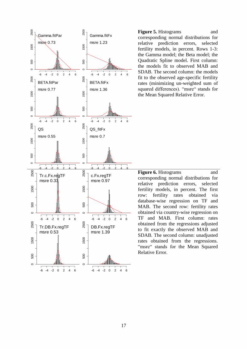
The above results suggesting unique importance of MAB in shaping the accuracy of

the predicted number of births bring us to the next research question addressed in Figures 5

and 6: might it be better to predict the MAB explicitly and not indirectly through modeling

the whole age pattern of Fx? In Figure 5, errors of the Gamma, Beta, and Quadratic Spline

models are presented for two variants of model fitting: to the MAB and SDAB (the left

column) and to the whole age schedule of fertility rates (the right column). The first option (fit

to MAB and SDAB only, neglecting the fit to the whole age pattern of fertility rates) is

substantially better in terms of prediction errors. Fitting the Gamma or Beta models to Fx is,

against intuition, almost as bad as assuming rectangular fertility (despite clearly skewed shape

of the distributions, a closer examination of countries with higher prediction errors does not

reveal a clear-cut selection: even if dominated by less developed, high-fertility, younger-age

fertility countries, those countries also include developed and low-fertility cases). Fitting to

MAB and SDAB, on the other hand, even if producing poorer fit to Fx as a whole, yields

better forecasts highlighting once more importance of accuracy of MAB estimates.

Interestingly, the QS model performs better than the other two when fit to Fx (but still worse

than in the case when it is fit to MAB and SDAB). In Figure 6, we present results for

modeling the fertility rates through regressions on TF and MAB (country-wise in the first

row, database-wise in the second row). A simple regression on TFR and MAB produces

rather high prediction errors, especially when the regressions are estimated on the whole

database. Yet, when these approximations are adjusted to fit exactly to the empirical MAB

and SDAB, errors drop almost three-fold. A similar comparison (not shown in the figure)

when both the left and the right-hand columns are produced by replacing the true observed

MAB and SDAB by their estimates, obtained from country-wise regressions on TF and time,

show considerably higher errors that are, however, again lower when the MAB and SDAB are

modeled explicitly (MSRE’s 1.29 and 1.32 percent for country and DB-wise repression-based

Fx’s fit to MAB and SDAB) as compared to situation when they are not fit to MAB and

13

SDAB (MSRE’s 1.41, and 1.78 for country and DB-wise repression-based Fx’s not fit to

MAB and SDAB).

In Figure 7, we examine if breaking down the fertility model by birth order may affect

the prediction efficacy. Such rates are potentially interesting both due to their policy-

relevance but also because one may well expect that a more specified model may perform

better. We consider rates of the first kind (occurrence/exposure rates). Parity-specific

population exposures may have very irregular age patterns that may very much affect the

prediction errors. That is well illustrated in Figure 7, where the fertility models are similar to

our simple model where regressions-based age-specific fertility rates are transformed (1) in

order to fit exactly MAB and SDAB (these notions do not apply to parity-specific rates but

may be replaced by a similar concepts of average age and standard deviation form that age in

the age distribution of the o-e rates). As seen in the figure, working with parity-specific o-e

rates may increase the prediction errors beyond acceptable levels: the errors are measured in

dozens of percent, and even the MSRE’s reach levels of 10%. Modeling directly the parity-

specific o-e rates is better be avoided and, perhaps, replaced by models for the rates of the

second kind and/or by decompositions of total births into births by parity.

The above results were highlighting one aspect of fertility modeling at a time. Yet, in

practice, projections include multiple approximations and simplifications. Figure 8 shows

what would be the combined effect of most typical simplifications of the fertility model (the

left hand panel: a parametric model, Gamma in this case, abridged into five-year age groups,

with MAB and SDAB fixed at their country-specific averages), how does in compare to our

best-performing alternative model (the central panel: age specific fertility rates, single years

of age, obtained from country-wise regressions on TF and adjusted to fit MAB and SDAB

that are, in turn, obtained from country-wise regressions on TF and time), and what could

have been the ideal efficiency of the same model with perfect predictions of MAB and SDAB

(the right-hand panel). Remarkably, already the simple alternative proposed above might have

14

yielded half the errors of the common approach to fertility projection; and even better models

for MAB may potentially lead to eight-times lower errors as compared to current practices.

References

Alho J.M. 1992. The magnitude of error due to different vital processes in population

forecasts. International Journal of Forecasting 8(3): 301–314.

Ediev, D. M. 2013. Comparative importance of the fertility model, the total fertility, the mean

age and the standard deviation of age at childbearing in population projections.

Presented at IUSSP International Population Conference, August 26-31, 2013. Busan,

South Korea. http://www.iussp.org/en/event/17/programme/paper/3054

Eurostat. 2011. EUROPOP2010 - Convergence scenario. Accessed on 14-12-2012 at:

http://epp.eurostat.ec.europa.eu/statistics_explained/index.php/Population_projections

Hoem, J. M., Madsen, D., Nielsen, J. L., Ohlsen, E.-M., Hansen, H. O., and Rennermalm, B.

1981. Experiments in Modelling Recent Danish Fertility Curves. Demography 18(2):

231-244.

Human Fertility Collection. 2013. Max Planck Institute for Demographic Research

(Germany) and Vienna Institute of Demography (Austria). Available at

www.fertilitydata.org (data downloaded on 16.09.2013).

Human Fertility Database. 2013. Max Planck Institute for Demographic Research (Germany)

and Vienna Institute of Demography (Austria). Available at www.humanfertility.org

(data downloaded on 11.06.2013).

Schmertmann, C. P. 2003. A system of model fertility schedules with graphically intuitive

parameters. Demographic Research 9(5): 82-110.

U.S. Census Bureau. 2012. Methodology and Assumptions for the 2012 National Projections.

United Nations. 2013. World Population Prospects. The 2012 Revision. New York: United

Nations.

http://www.iussp.org/en/event/17/programme/paper/3054

http://epp.eurostat.ec.europa.eu/statistics_explained/index.php/Population_projections

http://www.fertilitydata.org/

http://www.humanfertility.org/

15

-6 -4 -2 0 2 4 6

0500

1500

2500

Tr.Fx.c.averMA

msre 2.16

-6 -4 -2 0 2 4 6

0500

1500

2500

Tr.Fx.c.MAregTF

msre 1.38

-6 -4 -2 0 2 4 6

0500

1500

2500

Tr.Fx.c.MASDregTF.t

msre 1.12

-6 -4 -2 0 2 4 6

0500

1500

2500

Rect

msre 1.57

-6 -4 -2 0 2 4 6

0500

1500

2500

Ryder

msre 2.29

Figure 1. Histograms and

corresponding normal distributions for

relative prediction errors, selected

fertility models, in percent. First

column: the original fertility rates

transformed to set the MAB at its

average value for a given country;

same, MAB set to its value

approximated via (country-wise)

regression on TF; same, with regression

on TFR and time. Second column: the

Rectangular fertility model; Ryder’s

pentapartite model. “msre“ stands for

the Mean Squared Relative Error.

-6 -4 -2 0 2 4 6

0500

1500

2500

Tr.Fx.c.averSD

msre 0.62

-6 -4 -2 0 2 4 6

0500

1500

2500

Tr.Fx.c.SDregTF

msre 0.37

-6 -4 -2 0 2 4 6

0500

1500

2500

Tr.Fx.c.SDregTF.t

msre 0.3

-6 -4 -2 0 2 4 6

0500

1500

2500

Rect

msre 1.57

-6 -4 -2 0 2 4 6

0500

1500

2500

Ryder

msre 2.29






transformed to set the SDAB at its

average value for a given country;

same, SDAB set to its value

approximated via (country-wise)

regression on TF; same, with regression

on TFR and time. Second column: the


pentapartite model. “msre“ stands for


16

-6 -4 -2 0 2 4 6

0500

1500

2500

Gamma

msre 0.75

-6 -4 -2 0 2 4 6

0500

1500

2500

BetaAdj

msre 0.78

-6 -4 -2 0 2 4 6

0500

1500

2500

Tr.c.Fx.regTF

msre 0.33

-6 -4 -2 0 2 4 6

0500

1500

2500

Rect

msre 1.57

-6 -4 -2 0 2 4 6

0500

1500

2500

Ryder

msre 2.29

-6 -4 -2 0 2 4 6

0500

1500

2500

QS

msre 0.55





column: the Gamma model; the Beta

model adjusted to fit exactly the

observed MAB and SDAB; fertility

rates obtained via country-wise

regression on TF and MAB, adjusted to

fit exactly the observed MAB and

SDAB. Second column: the


pentapartite model; Schmertmann’s

Quadratic Spline model. “msre“ stands

for the Mean Squared Relative Error.

-6 -4 -2 0 2 4 6

0500

1500

2500

Abridg.10

msre 1.3

-6 -4 -2 0 2 4 6

0500

1500

2500

Abridg.5

msre 0.45

-6 -4 -2 0 2 4 6

0500

1500

2500

Rect

msre 1.57






abridged into 10-year age groups;

same, five-year age groups. Second

column: the Rectangular fertility

model. “msre“ stands for the Mean

Squared Relative Error.

17

-6 -4 -2 0 2 4 6

0500

1500

2500

Gamma.fitPar

msre 0.73

-6 -4 -2 0 2 4 6

0500

1500

2500

BETA.fitPar

msre 0.77

-6 -4 -2 0 2 4 6

0500

1500

2500

QS

msre 0.55

-6 -4 -2 0 2 4 6

0500

1500

2500

Gamma.fitFx

msre 1.23

-6 -4 -2 0 2 4 6

0500

1500

2500

BETA.fitFx

msre 1.36

-6 -4 -2 0 2 4 6

0500

1500

2500

QS_fitFx

msre 0.7




fertility models, in percent. Rows 1-3:

the Gamma model; the Beta model; the

Quadratic Spline model. First column:

the models fit to observed MAB and

SDAB. The second column: the models

fit to the observed age-specific fertility

rates (minimizing un-weighted sum of

squared differences). “msre“ stands for


-6 -4 -2 0 2 4 6

0500

1500

2500

Tr.c.Fx.regTFmsre 0.33

-6 -4 -2 0 2 4 6

0500

1500

2500

Tr.DB.Fx.regTFmsre 0.53

-6 -4 -2 0 2 4 6

0500

1500

2500

c.Fx.regTFmsre 0.97

-6 -4 -2 0 2 4 6

0500

1500

2500

DB.Fx.regTFmsre 1.39




fertility models, in percent. The first

row: fertility rates obtained via

database-wise regression on TF and

MAB. The second row: fertility rates

obtained via country-wise regression on

TF and MAB. First column: rates

obtained from the regressions adjusted

to fit exactly the observed MAB and

SDAB. The second column: unadjusted

rates obtained from the regressions.

“msre“ stands for the Mean Squared

Relative Error.

18

-20 -10 0 10 20

050

100

150

200

Tr.Fx.regr.MA.SD

msre 1.3

-20 -10 0 10 20

050

100

150

200

o_e_Fx1

msre 5.5

-20 -10 0 10 20

050

100

150

200

o_e_Fx2

msre 3.1

-20 -10 0 10 20

050

100

150

200

o_e_Fx3

msre 9.7

-20 -10 0 10 20

050

100

150

200

o_e_Fx4

msre 10.9

-20 -10 0 10 20

050

100

150

200

o_e_Fx5p

msre 9.9




fertility models, parity-specific o/e

rates, based on HFD data, in percent.

The first model: all parities combined.

Other boxes: parities 1 to 5+. In all

models, Center and Standard deviation

of the age distributions of rates are

estimated via regressions on Totals of

rates and on time (country-wise), and

the regressions-based rates are adjusted

to fit the estimated central age and

deviation. “msre“ stands for the Mean

Squared Relative Error.

-10 -5 0 5 10

0500

1000

1500

2000

2500

Gamma.averMA.SD.abridg5

msre 2.37

-10 -5 0 5 10

0500

1000

1500

2000

2500

Tr.Fx.regr.MA.SD

msre 1.27

-10 -5 0 5 10

0500

1000

1500

2000

2500

Tr.Fx.actual.MA.SD

msre 0.33

Figure 8. Prediction errors: current practices (the left-hand panel: a parametric model,

Gamma in this case, abridged into five-year age groups, with MAB and SDAB fixed at their

country-specific averages) vs suggested alternative (the central panel: age specific fertility

rates, single years of age, obtained from country-wise regressions on TF and adjusted to fit

MAB and SDAB that are, in turn, obtained from country-wise regressions on TF and time) vs

the suggested model under perfect predictions of MAB and SDAB (the right-hand panel).

19

Table 1. Mean squared relative errors of the predicted number of births for selected models and approximations, by database, in per cent.

Source of bias: Contributes %% error, by Database:

HFD RDD HFC EUSt WPP Merged DBa

MAB (country-wise regression on TFR + Calendar Year) 1.1 0.6 1.2 0.6 1.0 1.2

SDAB (country-wise regression on TFR+MAB+Calendar Year) 0.3 0.2 0.3 0.2 0.3 0.3

Fx model (country-wise regression on TFR, transformed to fit MAB, SDAB) 0.2 0.2 0.3 0.1 0.3 0.3

All of the above approximations combined together 1.3 0.6 1.3 0.7 1.0 1.3

MAB (country-wise regression on TFR) 1.4 1.0 1.4 1.3 1.3 1.4

SDAB (country-wise regression on TFR+MAB) 0.3 0.3 0.3 0.2 0.4 0.4

Time-constant MAB (fixed at country-wise average observed value) 1.6 1.3 2.0 1.5 2.2 2.2

Abridging in 5-year age groups 0.5 0.5 0.6 0.5 0.4 0.5

Abridging in 10-year age groups 1.5 1.5 1.3 1.4 1.3 1.3

Gamma model 0.7 0.9 0.8 0.6 0.7 0.7

Beta model (adjusted to fit MAB and SDAB) 0.7 1.0 0.8 0.5 0.8 0.8

Country-wise regression of Fx on TFR and MAB 0.3 0.5 0.6 0.2 1.1 1.0

same, adjusted to fit MAB and SDAB exactly 0.2 0.2 0.3 0.1 0.3 0.3

Database-wise regression of Fx on TFR and MAB 0.8 0.8 1.0 0.8 1.5 1.4

same, adjusted to fit MAB and SDAB exactly 0.4 0.4 0.4 0.3 0.6 0.6

Rectangular model 1.5 2.0 1.7 1.3 1.5 1.6

Ryder’s 5-partite model 1.9 2.0 1.8 1.8 2.8 2.3

* HFD=human Fertility Database, RDD=Recent Demographic Developments report (2005), HFC=Human fertility Collection, EUSt=Eurostat’s estimates,

WPP= UN’s World Population Prospects 2012 report. a Includes, with duplications cleaned, (in the priority order): HFD, RDD, HFC, EUSt, WPP.

20

Table 2. Mean squared relative errors of the predicted number of births, selected models and parameterizations, merged database, in per cent.

MAB

approximation

SDAB

approximation

Direct

trans-

formation

of the

fertility

schedule

Same,

abridged

in 5-year

age

groups

Same,

abridged

in 10-year

age

groups

Country-

wise

regressions-

based

fertility

schedule

Same,

adjusted

to fit

assumed

MAB and

SDAB

DB-wise

regressions-

based

fertility

schedule

Same,

adjusted

to fit

assumed

MAB and

SDAB

Schmert-

mann’s

Quadr.

Spline

model

Gamma

model Same,

abridged

in 5-year

age

groups

Beta

model,

adjusted

to fit

MAB and

SDAB

Rectan-

gular

model

Ryder’s

penta-

partite

model

exact value exact value 0.0 0.5 1.3 1.0 0.3 1.4 0.5 0.6 0.7 0.9 0.8 1.6 2.3

exact value country average 0.6 0.7 1.4 1.0 0.7 1.4 0.8 0.8 1.0 1.0 1.0 1.6 2.1

exact value country regression

(~TF+MAB) 0.4 0.6 1.4 1.0 0.5 1.4 0.6 0.7 0.8 0.9 0.9 1.6 2.3

exact value country regression (~TF+MAB+time)

0.3 0.6 1.3 1.0 0.5 1.4 0.6 0.6 0.8 0.9 0.8 1.6 2.3

exact value DB-regression

(~TF+TF^2+MAB) 0.7 0.8 1.5 1.0 0.8 1.4 0.9 0.9 1.0 1.1 1.1 1.7 2.4

country average exact value 2.2 2.2 2.6 3.1 2.3 2.5 2.3 2.4 2.4 2.4 2.4 2.7 3.1 country regression

(~TF) exact value 1.4 1.5 1.9 1.6 1.5 1.9 1.5 1.6 1.7 1.6 2.1 2.7

country regression

(~TF+time) exact value 1.2 1.2 1.7 1.4 1.3 1.8 1.3 1.6 1.4 1.5 1.4 2.0 2.6

DB-regression

(~TF+TF^2) exact value 3.2 3.2 3.4 5.4 3.7 3.3 3.3 3.3 3.4 3.4 3.4 3.6 3.8

country average country average 2.1 2.1 2.5 3.1 2.3 2.5 2.2 2.3 2.3 2.4 2.3 2.6 3.0 country regression

(~TF)

country regression

(~TF+MAB) 1.3 1.4 1.9 1.6 1.5 1.9 1.5 1.6 1.7 1.6 2.1 2.7

country regression

(~TF+time)

country regression

(~TF+MAB+time) 1.1 1.2 1.7 1.4 1.3 1.8 1.3 1.5 1.4 1.5 1.4 2.0 2.6

DB-regression (~TF+TF^2)

DB-regression (~TF+TF^2+MAB)

3.1 3.2 3.3 5.4 3.7 3.3 3.3 3.3 3.4 3.4 3.4 3.6 3.9

TFR’s mean squared annual change

(%) 4.23

contribution of fertility model and parameterization …...mortality assumptions as up to 0.02...

Documents