contributions to multivariate control charting

CONTRIBUTIONS TO MULTIVARIATE CONTROL CHARTING:

STUDIES OF THE Z CHART AND FOUR

NONPARAMETRIC CHARTS

by

JEFFREY MICHAEL BOONE

A DISSERTATION

Submitted in partial fulfillment of the requirements for the

degree of Doctor of Philosophy in the Department of

Information Systems, Statistics, and Management

Science in the Graduate School of

The University of Alabama

TUSCALOOSA, ALABAMA

2010

Copyright Jeffrey Michael Boone 2010

ALL RIGHTS RESERVED

ii

ABSTRACT

Autocorrelated data are common in today‟s process control applications. Many of these

applications involve two or more related variables so that multivariate statistical process control

(SPC) methods should be used in process monitoring since the relationship among the variables

should be accounted for. Dealing with multivariate autocorrelated data poses many challenges.

Even though no one chart is best for multivariate data, the Z chart proposed by Kalgonda and

Kulkarni (2004) is fairly easy to implement and is particularly useful for its diagnostic ability,

which is to pinpoint the variable(s) that is(are) out of control in case the chart signals. In this

dissertation, the performance of the Z chart is compared to Hotelling‟s χ2 chart and the

multivariate EWMA (MEWMA) chart in a number of simulation studies. Simulations are also

performed to study the effects of parameter estimation and non-normality (using the multivariate

t and multivariate gamma distributions) on the performance of the Z chart.

In addition to the problem of autocorrelation in multivariate quality control, in many

quality control applications, the distribution assumption of the data is not met or there is not

enough evidence showing that the assumption is met. In many situations, a control chart that

does not require a strict distribution assumption, called a nonparametric or distribution-free chart,

may be desirable. In this paper, four new multivariate nonparametric Shewhart control charts are

proposed. They are relatively simple to use and are based on the multivariate forms of the sign

and Wilcoxon signed-rank statistics and the maximum of multiple univariate sign and Wilcoxon

signed-rank statistics. The performance of these charts is also studied. Illustrations and

applications are also demonstrated.

iii

ACKNOWLEDGEMENTS

I am pleased to have the opportunity to thank everyone who helped me in the

development of this dissertation. I would first like to thank my dissertation chairman, Dr.

Subhabrata Chakraborti, who was very helpful in instructing me with the research process long

before beginning the dissertation. Without his help and diligence to ensure the best quality of

work, this work would not have been nearly as acceptable. I would also like to thank the other

members of my committee, Dr. Marcus Perry, Dr. Brian Gray, Dr. David Miller, and Dr. Junsoo

Lee, as well as all my other professors, for all of their help.

The financial assistance that I received from Dr. Michael Conerly and the ISM

Department, as well as the graduate school, made my graduate career here possible.

My fellow graduate students also proved very helpful during my graduate career. I would

especially like to thank Amanda McCracken and Hervé Dovoedo for all of their support with

coursework and for being great friends.

I am also very thankful for the support of the faculty and staff of the Department of

Mathematics and Statistics and the Department of Philosophy at the University of South

Alabama. Dr. Madhuri Mulekar and Dr. Satya Mishra, along with the rest of the department,

fueled my interest in the area of statistics.

Finally, I would like to thank my parents, Jeff Boone and Brenda Beeson, and my sister,

Stephanie McGrew, for all the support they have provided throughout my entire life. I am also

entirely grateful for the overwhelming support of my wife, Ashley Singleton. Without her none

of this would be possible.

iv

CONTENTS

ABSTRACT .................................................................................................................................... ii

ACKNOWLEDGEMENTS ........................................................................................................... iii

LIST OF TABLES ......................................................................................................................... ix

LIST OF FIGURES ....................................................................................................................... xi

1. INTRODUCTION .......................................................................................................................1

1.1 Overview of Control Charts .....................................................................................1

1.2 Multivariate Control Charts .....................................................................................2

1.3 Control Charts for Autocorrelated Data ...................................................................6

1.3.1 Univariate .....................................................................................................6

1.3.2 Multivariate ..................................................................................................7

1.4 Nonparametric Control Charts .................................................................................9

1.4.1 Univariate .....................................................................................................9

1.4.2 Multivariate ................................................................................................13

1.5 Focus of Dissertation .............................................................................................13

1.5.1 Performance Comparison of the Z Chart ...................................................13

1.5.2 Effects of Parameter Estimation on the Performance of the Z Chart ........14

1.5.3 Robustness of the Z Chart to the Assumption of Multivariate

Normality ...................................................................................................15

1.5.4 Four Nonparametric Multivariate Control Charts and Their

Performance ...............................................................................................16

1.5.5 Applications to Real Data ..........................................................................16

v

1.5.6 Layout of Dissertation................................................................................17

2. LITERATURE REVIEW ..........................................................................................................18

2.1 Multivariate Control Charts ...................................................................................18

2.1.1 Hotelling‟s χ2 and T

2 control charts ...........................................................18

2.1.2 The Multivariate Exponentially-Weighted Moving Average

Control Chart .............................................................................................22

2.1.3 The Multivariate Cumulative Sum Control Chart .....................................23

2.1.4 Other Multivariate Techniques ..................................................................23

2.2 Control Charts for Univariate Autocorrelated Data ...............................................25

2.2.1 Univariate ...................................................................................................25

2.2.2 Multivariate ................................................................................................26

2.2.2.1 The Z Chart .................................................................................28

2.3 Nonparametric Control Charts ...............................................................................30

2.3.1 Univariate ...................................................................................................30

2.3.2 Multivariate ................................................................................................31

2.4 Robustness of Control Charts ................................................................................32

2.4.1 Robustness to the Assumption of the Underlying Distribution .................33

2.4.2 Robustness to the Estimation of Parameters ..............................................34

2.5 Summary ................................................................................................................36

3. PERFORMANCE COMPARISON OF THE Z CHART ..........................................................37

3.1 Introduction ............................................................................................................37

3.2 Simulation ..............................................................................................................41

3.3 Conclusions ............................................................................................................44

3.4 Future Work ...........................................................................................................46

vi

4. THE EFFECT OF PARAMETER ESTIMATION ON THE PERFORMANCE

OF THE Z CHART ....................................................................................................................48

4.1 Introduction ............................................................................................................48

4.2 Regression Approach to UCL Estimation..............................................................51

4.3 Estimation Procedures ...........................................................................................52

4.4 Simulation ..............................................................................................................55

4.5 Results and Conclusions ........................................................................................60

5. THE ROBUSTNESS OF THE Z CHART TO THE ASSUMPTION OF

MULTIVARIATE NORMALITY ............................................................................................62

5.1 Introduction ............................................................................................................62

5.2 Simulation ..............................................................................................................64

5.3 Results and Conclusions ........................................................................................68

6. SOME SIMPLE MULTIVARIATE NONPARAMETRIC CONTROL CHARTS ..................70

6.1 Introduction ............................................................................................................70

6.2 Shewhart-Type Charts ...........................................................................................74

6.2.1 The Multivariate Sign Control Chart .........................................................74

6.2.2 The Multivariate Signed-Rank Control Chart............................................76

6.3 Charts Based on the Maximum of Multiple Univariate Nonparametric

Statistics .................................................................................................................78

6.3.1 The Maximum Sign Chart .........................................................................78

6.3.2 The Maximum Wilcoxon Signed-Rank Chart ...........................................80

6.4 Example .................................................................................................................82

6.5 Performance Study .................................................................................................84

6.5.1 Simulation ..................................................................................................84

6.5.2 In-Control Performance .............................................................................87

vii

6.5.3 Out-of-Control Performance ......................................................................92

6.6 Conclusions and Recommendations ......................................................................98

7. APPLICATION TO REAL DATA .........................................................................................101

7.1 Introduction ..........................................................................................................101

7.2 Application of the Z Chart ...................................................................................101

7.2.1 Description of Data ..................................................................................101

7.2.2 Results ......................................................................................................104

7.3 Application of the New Nonparametric Charts ...................................................106

7.3.1 Description of Data ..................................................................................106

7.3.2 Results ......................................................................................................109

7.4 Conclusions ..........................................................................................................114

8. CONCLUSION ........................................................................................................................115

8.1 Summary ..............................................................................................................115

8.2 Future Research ...................................................................................................117

REFERENCES ............................................................................................................................118

APPENDIX ..................................................................................................................................125

Appendix A The Multivariate t Distribution ................................................................125

Appendix B The Multivariate Gamma Distribution .....................................................127

Appendix C R Programs Used for Simulation .............................................................130

C.1 Programs for Chapter 3 ............................................................................130




viii

C.4.1 Multivariate Sign Chart Programs ...............................................144

C.4.2 Multivariate Signed-Rank Chart Programs ..................................151

C.4.3 Maximum Sign Chart Programs ..................................................157

C.4.4 Maximum Signed-Rank Chart Programs .....................................162


ix

LIST OF TABLES

3.1 Simulation results for VAR(1) data using the autocorrelation matrix .........................43



4.1 In-control results ................................................................................................................56

4.2 Out-of-control results .........................................................................................................58

5.1 In-control run length of the Z chart for various distributions using UCL=2.781 ..............66

5.2 Out-of-control results .........................................................................................................67

6.1 Values of the charting statistics .........................................................................................82

6.2 Upper control limits for simulation....................................................................................86

6.3 In-control run length using the asymptotic distribution .....................................................87

6.4 Multivariate sign and signed-rank charts with using the asymptotic

control limits ......................................................................................................................91

6.5 Maximum sign and signed-rank charts with using the asymptotic

control limits ......................................................................................................................91

6.6. Multivariate sign and signed-rank charts with multivariate normal data with

ARL0 set to 200 ..................................................................................................................94

6.7 Multivariate sign and signed-rank charts with multivariate t data with 5

degrees of freedom with ARL0 set to 200 ..........................................................................94

6.8 Multivariate sign and signed-rank charts with multivariate t data with 10


6.9 Maximum sign and signed-rank charts with multivariate normal data with

ARL0 set to 200 ..................................................................................................................95

x

6.10 Maximum sign and signed-rank charts with multivariate t data with 5


6.11 Maximum sign and signed-rank charts with multivariate t data with 10


A.1 Skewness and kurtosis for univariate t distributions........................................................126

B.1 Skewness and kurtosis for univariate Gamma distributions ............................................129

xi

LIST OF FIGURES

1.1 Example of a bivariate normal distribution .........................................................................3

1.2 Individuals chart applied to autocorrelated data ..................................................................7

1.3 Hotelling's T2 chart applied to in-control autocorrelated data .............................................9

1.4 Individuals chart applied to an Exponential (1) process ....................................................12

1.5 Individuals chart applied to a Laplace (0,1) process ..........................................................12

3.1 MEWMA chart applied to data ..........................................................................................45

3.2 Z chart applied to data........................................................................................................45

3.3 Z statistic for first variable .................................................................................................46

3.4 Z statistic for second variable ............................................................................................46

4.1 Predicting UCL for ARL0=200 ..........................................................................................52

4.2 ARL0 for different estimating sample sizes .......................................................................56

4.3 SDRL for different estimating sample sizes ......................................................................56

4.4 MRL for different estimating sample sizes ........................................................................57

5.1 Normal probability plot of t(5) data ...................................................................................69

6.1 Multivariate sign chart .......................................................................................................82

6.2 Multivariate signed-rank chart ...........................................................................................82

6.3 Maximum sign chart ..........................................................................................................83

6.4 Maximum signed-rank chart ..............................................................................................83

6.5 Maximum sign chart for individual variables ....................................................................83

6.6 Maximum signed-rank chart for individual variables ........................................................83

xii

6.7 ARL0 for MVN data for each chart....................................................................................88

6.8 ARL0 for MVT(5) data for each chart ...............................................................................88

6.9 ARL0 for MVT(10) data for each chart .............................................................................89

7.1 Time series plot of flow rate ............................................................................................102

7.2 Time series plot of power ................................................................................................102

7.3 Time series plot of flow rate and power ..........................................................................102

7.4 Histogram of flow rate .....................................................................................................103

7.5 Histogram of power .........................................................................................................103

7.6 Normal probability plot of flow rate ................................................................................103

7.7 Normal probability plot of power ....................................................................................103

7.8 Z chart applied to the hydroelectric data ..........................................................................105

7.9 Plot of Z for flow rate ......................................................................................................106

7.10 Plot of Z for power ...........................................................................................................106

7.11 Time series plot of the means of pressure ........................................................................107

7.12 Time series plot of the means of temperature ..................................................................107

7.13 Time series plot of pressure and temperature means .......................................................107

7.14 Histogram of pressure ......................................................................................................108

7.15 Histogram of temperature ................................................................................................108

7.16 Normal probability plot of pressure (individual values) ..................................................109

7.17 Normal probability plot of temperature (individual values) ............................................109

7.18 Hotelling‟s T2 chart of pressure and temperature ............................................................110

7.19 Multivariate sign chart applied to the phase II process data ............................................111

7.20 Multivariate signed-rank chart applied to the phase II process data ................................111

xiii

7.21 Maximum sign chart applied to the phase II process data ...............................................112

7.22 Maximum signed-rank chart applied to the phase II process data ...................................112

7.23 Plot of univariate signed-rank statistics for pressure .......................................................113

7.24 Plot of univariate signed-rank statistics for temperature .................................................113

1

CHAPTER 1

INTRODUCTION

1.1 Overview of Control Charts

Statistical process control (SPC) is involved with continuous monitoring or surveillance

of a process. This may include, for example, monitoring some quality characteristics of

manufactured items to ensure their adherence to certain standards, the ongoing surveillance of

health data to detect an outbreak of a disease, or the observance of a natural phenomenon such as

water salinity levels. An important tool for the monitoring of quality is the control chart. First

introduced by Walter Shewhart in 1924, the control chart has become a major topic of research

in multiple fields.

Control charts are statistical and visual tools designed to detect changes in a process. A

process that is operating at or around some target value and only under some random variation

(so-called common causes) is called an in-control process and is denoted IC. A process that has

somehow changed from its in-control state is said to be out-of-control and is denoted OOC.

Various parameters of a process may be of interest in different situations: the central tendency is

one of the most common as is the spread or the variation. A control chart is formed by plotting a

certain statistic over time. A center line is plotted in the graph showing the expected value of the

statistic when the process is in control, along with an upper and a lower control limit. The control

chart signals when the plotted statistic falls either above or below the control limit. The control

limits are obtained using the distribution of the charting statistic and the desired false alarm rate

2

(similar to the probability of a Type-1 error in hypothesis testing). When a signal is indicated, the

process may not have actually gone out of control. However, the practitioner might suspect that a

change has occurred in the process and an investigation is started as to the cause of the signal.

This dissertation will focus on detecting shifts in the central tendency of a process.

The statistical process control (SPC) regime is usually split into two phases, namely

phase I and phase II, as explained in Montgomery (2005). Phase I constitutes a retrospective

study where exploratory work is done including estimating any unknown parameters and

calculating the control limits to establish if a process is in control. Once this is achieved, the in-

control (reference) data are used in phase II to monitor the process. This dissertation will mostly

focus on phase II control charts and their performance.

1.2 Multivariate Control Charts

Consider testing whether a specified value of the mean of a process is plausible. In the

hypothesis testing context, a univariate test, such as a t-test, may be used for this purpose. If

multiple variables are present, multiple univariate tests may be performed to determine the

plausibility of each of the values for the means. However, it may be the case that a relationship

exists between the variables of interest and if so, a multivariate testing method for the mean

vector would be a better statistical procedure. For example, if a quality control technician is

monitoring the length, width, and diameter of a manufactured item and is interested in knowing

whether or not the process is in control, a multivariate formulation of the problem is more

meaningful since the characteristics in question would be correlated.

An example of a bivariate distribution can be seen below in Figure 1.1. A 95%

confidence ellipse has been drawn on the plot. Notice that due to the correlation between the two

3

variables, an ellipse is used. If no correlation exists between the variables, two univariate

confidence intervals, one for each of the means of variables, respectively, could be used to

determine if a given observation is in control (reasonable) or not (out of control). A common

example of the importance of taking account of the multivariate structure of the variables

involves the relationship between the height and weight of a person. Assuming that a 95%

confidence interval for the mean weight of the population is (100lbs, 200lbs) and a 95%

confidence interval for the mean height of the population is (60in, 72in), a person with a weight

of 110lbs and a height of 71in would fall within the respective confidence intervals, suggesting

that it is not uncommon for a person to weigh 110lbs and to be 71 inches tall. Together however,

it seems strange that a 71 inches tall person would weigh only 110lbs. Hence if both height and

weight are considered to determine if the point is in control (common or typical) or not

(unusual), the individual confidence intervals would not be appropriate and a bivariate

confidence ellipse should be considered.

Figure 1.1: Example of a bivariate normal distribution.

The concept extends easily to statistical process control. While monitoring a process,

variables or attributes are often monitored separately. However, if the variables are related to one

4

another, this may not be the best strategy and multivariate methods should be considered as using

information from multiple variables together (simultaneously) may provide a better (more

efficient) monitoring procedure. Similar to the height and weight example above, the variables

being monitored may be in control in their respective individual control charts, but may not be in

control when viewed simultaneously, i.e., a multivariate chart may show that the process is not in

control while the univariate charts show there is no reason for concern.

An example of a multivariate quality control problem can be seen in Montgomery (2005).

A quality engineer is monitoring a textile fiber manufacturing process. The tensile strength and

diameter of the fibers are measured. Since these two quality characteristics are probably highly

correlated, two individual univariate charts may not be the best choice in monitoring the process.

This would then be considered a multivariate process. A multivariate control chart is then

applied to the process and the process is monitored.

It should be noted that when monitoring several variables separately one needs to be

careful about maintaining the overall false alarm rate (probability), FAP, defined as the

probability of at least one false alarm. The problem is similar to the problem arising in multiple

comparisons. If individual α-level (false alarm rate α) charts are used to monitor the variables,

the FAP (also called the experiment-wise error rate in hypothesis testing) would not be

maintained at α. If p individual α-level charts are used and the variables are independent, the

FAP is equal to , which is typically much greater than . For example, if the

desired false alarm rate is and two independent variables are monitored

simultaneously, the FAP is equal to , (which is roughly

twice that of 0.005) and therefore many more false alarms are expected. The situation gets worse

when more variables are monitored, for example, for ,

5

. So, if individual control charts are to be used, they should

each be adjusted to have level . Otherwise, the control limits will be set

incorrectly and this may lead to the charting statistics falling inside (or outside) the control limits

when in fact they should not be. Even when the control limits are adjusted for multiplicity, as

explained earlier, individual monitoring is not preferable when the variables are related and

multivariate SPC methods are recommended.

Some practitioners may feel discouraged to use multivariate SPC methods. One major

reason for this is the issue with the interpretation of an OOC signal. When a multivariate control

chart signals, it implies that at least one of the variables is OOC but it does not necessarily

indicate which one or which ones. Wetherill and Brown (1991), among others, point out that

many multivariate methods give “no indication of which variable or variables are causing the

problem.” Few multivariate charts can determine which variable or variables are OOC unless

further analysis is done. However, recent work has been done to determine the variable or

variables that led to the multivariate OOC signal. Some of these can be seen in the following

chapter. A common method used in a post-signal analysis is to run multiple univariate charts and

see which variables signal on the individual charts. However, this is inappropriate since as noted

earlier, using multiple univariate charts would not control the overall false alarm rate, possibly

leading to more false alarms, as also noted by Hayter and Tsui (1994). The bottom line is that if

too many false alarms occur, there will be loss of time and resources along with the confidence

among the practitioners using such methods. The construction of multiple univariate charts

would also not use the information in the correlation between the variables. Ignoring this

correlation can lead to incorrect control limits (Mason, Champ, Tracy, Wierda, and Young,

1997).

6

1.3 Control Charts for Autocorrelated Data

1.3.1 Univariate

In both classical univariate and multivariate SPC problems, successive observations or

samples of observations are assumed to be statistically independent. This, however, may not be

the case in many of today‟s quality control applications. A simple example where the

independence assumption is violated is where the variable being monitored is correlated with

itself over time. Such variables are called autocorrelated and such data are referred to as

autocorrelated data. This autocorrelation may arise due to some natural reason or may be due to a

very rapid sampling procedure used for example in today‟s highly automated production

environments. It has been shown that the failure to account for such autocorrelation may lead to

too many false alarms, particularly in the case of positive autocorrelation (Montgomery 2005).

To deal with this situation, several approaches have been proposed. If the autocorrelation is due

to rapid sampling, one can sample less frequently. This, however, can be a bad decision since we

would not be able to detect a change in the process very quickly if the time interval is too wide.

Box, Jenkins, and Reinsel (2008) state that “we want the interval to be such that not too much

change can occur during the sampling interval.” Researchers have also developed control charts

to handle autocorrelated data. Some of these charts are applied directly to the data. Others

require a time series model, such as an autoregressive integrated moving average (ARIMA)

model, to be first fit to the data and then monitoring the residuals from the fitted model. Some of

these charts will be discussed in the next chapter.

An example of a case of autocorrelated data can be found in Montgomery (2005). One

variable, viscosity, is measured during a chemical process. This variable is highly related to itself

over time, and this can be seen by the time series plot showing the viscosity values appearing to

7

“drift or wander slowly over time.” Due to the autocorrelated nature of the process, a common

univariate chart for non-autocorrelated data applied directly to the data will not provide the

desired results. An individuals chart applied to the data shows too many false signals and proves

to be inadequate for monitoring the data. An individuals chart applied to simulated data from an

AR(1) model can be seen below in Figure 1.2. Although the data were simulated in the in-control

state (no shift in the process mean), the individuals chart proves to be misleading. The chart

shows the process going away from its in-control state near time point 10 but then going back to

the in-control state near time point 34. However the process never actually left its in-control

state.

Figure 1.2: Individuals chart applied to autocorrelated data.

1.3.2 Multivariate

Either of the two issues, monitoring several variables (multivariate/multiplicity)

simultaneously and the autocorrelation (variables correlated over time) within the variables, can

spell trouble for the quality engineer. To make matters worse, these problems may be present

together in certain applications. The quality engineer may be monitoring multiple correlated

8

variables that individually have some autocorrelation. So here, the correlation between the

variables as well as the autocorrelation within each variable should be considered. As in the

univariate case, it is clear that typical multivariate charts for i.i.d. data may not be appropriate for

monitoring multivariate autocorrelated data. As has been done in the univariate case (see

Vasilopoulos and Stamboulis 1978), one approach would be to widen the control limits designed

for multivariate i.i.d. data to account for the autocorrelation. Another approach, again similar to

the univariate case, would be to fit a model and monitor the residuals. For example, an ARIMA

model may be developed for each variable, the residuals obtained, and a multivariate model

applied to monitor the residuals of each. A third option would be instead of fitting an univariate

ARIMA model to each variable, its multivariate analog, the vector ARIMA (VARIMA) model,

would be fit to the multivariate data and the corresponding residuals monitored. However, the

model-based approaches suffer a disadvantage in that the (VARIMA or ARIMA) fitted model is

assumed to be the correct one describing the data.

Other charts have been developed to be applied directly to the data as well. Applying a

multivariate chart directly to the multivariate autocorrelated data yields problems similar to the

case of univariate autocorrelated data: the control limits are often specified incorrectly. In Figure

1.3 below, a Hotelling‟s T2 control chart is applied directly to data simulated from a VAR(1)

model. The process shows a diversion from its in-control state near time point 10 and seems to

return to the in-control state near time point 34. However, it never actually left its in-control

state.

9

Figure 1.3: Hotelling's T

2 chart applied to in-control autocorrelated data.

1.4 Nonparametric Control Charts

1.4.1 Univariate

It has been noted that (e.g., Woodall and Montgomery, 1999) the control charting

methodology shares similarities with classical statistical inference methods such as hypothesis

testing and confidence intervals. Many statistical inference procedures are derived under the

assumption that the variable(s) under study follows some specific parametric distribution. These

are called parametric inference procedures. Such procedures are then optimal and most efficient

when in fact that distributional assumption is true and the conclusions reached via these

procedures are only “exactly valid only so long as the assumptions themselves can be

substantiated” (Gibbons and Chakraborti, 2003). However, the reality is that such information is

seldom, if ever, available to the practitioner trying to solve the problem. To overcome this issue,

statistical inference procedures, including hypothesis tests, confidence intervals, and control

charts that do not require making any specific parametric distributional assumptions have been

464136312621161161

160

140

120

100

80

60

40

20

0

Time

Tsq

ua

red

Median=2.2

UCL=17.2

Hotelling's T-squared Chart

10

proposed and studied. Collectively, these techniques are called nonparametric or distribution-free

techniques.

There is a large body of literature on nonparametric tests and confidence intervals. Many

of these methods use the ranks of the data as well as the order statistics, such as the minimum,

median, and maximum. Two simple and popular examples of nonparametric tests are the

Wilcoxon signed-rank test and the sign test. Either of these can be used as an alternative to the

one sample and the paired sample Z test (and t test) in determining if a certain value of the

location (the mean or the median) is plausible. Instead of working with the actual (magnitudes of

the) data, these tests use the rank of each data value and/or the sign of that value (positive if it

exceeds the hypothesized median) in the calculation of the statistic. For comparing two

population locations, the Wilcoxon rank-sum test is a popular alternative to the two-sample Z

test and the two-sample t test. These and other nonparametric procedures may be adapted and

applied to SPC to construct control charts that do not require the assumption of a parametric

distribution and are therefore robust to the assumption of a distribution.

When the distributional assumptions underlying a parametric control chart are violated,

the performance of the control chart often deteriorates and a nonparametric control chart may

provide a better alternative. If a parametric control chart is used on data that do not follow the

assumed distribution under which the chart is constructed, the signals (or the lack thereof) given

by that chart, may be erroneous. An argument is often made against the use of nonparametric

control charts (as well as nonparametric hypothesis tests) is that the power of the chart (or test) is

not as high as the power of a parametric chart (or test). This is, of course, true when the

distributional assumptions for the parametric chart are exactly satisfied. However, as we said

11

before, in practice it is rare to expect that the assumptions will be exactly met or in fact that such

information will be available to the practitioner.

As an example, suppose that a process follows a non-normal distribution and yet a set of

Shewhart control limits designed to be used with normally distributed data are applied for

process monitoring. To see the effects of this incorrect decision process, two sets of in-control

data are generated from an Exponential(1) and a Laplace(0,1) distribution. The Laplace(0,1)

distribution is a (standard) normal-like distribution (symmetric at 0) but heavier in the tails, with

a variance of 2. The Exponential(1) distribution is a very skewed distribution with a mean and

variance of 1. Using a false-alarm rate of 0.005 (desired in-control ARL of 200), individuals

charts are applied to these (in-control) data. The charts can be seen in Figures 1.4 and 1.5. For

the skewed case of Exponential(1) data, the process signals three times (which may not be a

problem). However, note that since the distribution is skewed and the chart has symmetric

control limits, monitoring the process for values less than the mean is almost impossible using

this chart. For the less-extreme symmetric case of Laplace(0,1) data, the chart signals twice

(almost a third time as well) within the 50 observations. This demonstrates that the further the

process distribution is from the normal, the less appropriate these charts are and this

phenomenon could render such charts almost useless in practice.

12

Figure 1.4: Individuals chart applied to an Exponential (1) process.

Figure 1.5: Individuals chart applied to a Laplace (0,1) process.

On the other hand, to re-emphasize the point, the false alarm rates of nonparametric charts will

not be influenced by the underlying distributions.

13

1.4.2 Multivariate

Many multivariate techniques, just as their univariate counterparts, rely on certain

distributional assumptions. As in the univariate case, if these assumptions cannot be properly

justified, or are not true, the results and the conclusions of the corresponding inference

procedures may not be valid. With this motivation, multivariate forms of some nonparametric

techniques have been developed in the literature. Two of the more popular ones are the

multivariate Wilcoxon signed-rank test and the multivariate sign test. The critical values for

these tests may be obtained using the asymptotic distribution or by simulation.

Again, as in the univariate case, multivariate nonparametric tests can be adapted to

develop multivariate control charts. When the multivariate distribution assumption of a

multivariate control chart is violated or unjustifiable, the signals and the conclusions from the

parametric chart become questionable. Nonparametric multivariate control charts can provide

better alternatives in such situations. Although several nonparametric control charts have been

introduced for use with univariate data, few nonparametric control charts currently exist for

multivariate data. A review of some of these techniques can be seen in the next chapter.

1.5 Focus of Dissertation

1.5.1 Performance Comparison of the Z chart

One focus of this study is the performance of the Z chart presented by Kalgonda and

Kulkarni (2004). The Z chart has the practical advantage of diagnostic ability, to indicate which

variables are OOC following a signal, but a thorough study needs to be performed to determine

how well the chart performs in the presence of autocorrelation. The performance of the Z chart

will be compared with the multivariate exponentially-weighted moving average (MEWMA)

14

control chart and Hotelling‟s χ2 control chart. These two charts are chosen since the MEWMA is

often used for its ability to detect smaller shifts in the process mean vector and the Hotelling‟s

χ2chart is often used for its simplicity and ability to detect larger shifts quickly. The multivariate

cumulative sum (MCUSUM) control charts are not used in the study since it has been shown to

have similar performance as the MEWMA, such as in Champ and Jones-Farmer (2007), and with

the MEWMA already used in our comparisons, there will be little information gained by using

the MCUSUM chart. It may be noted that Hwarng and Wang (2008) recently used all three of

these charts in comparing their neural-network-based identifier chart. However, their control

limits were calculated under the assumption of no autocorrelation and independence and this

may have led to erroneous performance results and a misinterpretation of these results.

In this dissertation, three different autocorrelation matrices will be used to study the

effects of low, medium, and high autocorrelation on the performance of the control chart. The

distribution of the run length, including the average run length, median run length, standard

deviation of the run length, and other percentiles will be used as performance measures.

1.5.2 Effects of Parameter Estimation on the Performance of the Z Chart

While much of the performance comparisons assume known parameters, in practice some

or all of the process parameters (means, standard deviations, and autocorrelations) will be

unknown and need to be estimated from the data. There is evidence in the literature that control

chart performance degrades when estimated parameters are “plugged-in” and therefore there is a

need to study the effects of parameter estimation on the performance of the Z chart. To this end

data will be generated from a vector autoregressive (VAR) model where the error terms are i.i.d.

multivariate normal. The parameters required for the application of the Z chart will be estimated

15

from a section of the data and the Z chart will be applied to the latter section of the data. The

effect on the in-control ARL will be studied. To observe the out-of-control performance, the

UCL will be found by simulation to obtain a certain in-control ARL. The out-of-control

performance of the chart based on these limits will be noted and compared to the case where

parameters are known. The study will be similar in design to those of Champ, Jones-Farmer, and

Rigdon (2005) for Hotelling‟s T2control chart and Champ and Jones-Farmer (2007) for the

multivariate EWMA control chart and multivariate CUSUM control charts.

1.5.3 Robustness of the Z Chart to the Assumption of Multivariate Normality

In many situations in practice, the distributional assumption required for a control chart

may be violated or it might be difficult to verify. If the control chart requires the data to follow a

normal distribution (or some other specified distribution), the failure to do so generally has a

strong adverse effect on the performance of the control chart. This is particularly true for the in-

control performance of many charts, which makes their application and performance studies

rather questionable. This has been studied in several papers for different univariate control

charts. For example, Borror, Montgomery, and Runger (1999) examined the Shewhart X-bar and

the EWMA charts, and Shilling and Nelson (1976) compared a variety of charts. In the

multivariate setting, Stoumbos and Sullivan (2002) studied the MEWMA chart and Chou,

Mason, and Young (2001) studied the T2 chart. In the same spirit, we will examine the

performance of the Z chart from the point of view of robustness to a violation of the assumption

of multivariate normality. Simulations will be done to generate multivariate autocorrelated data

that violate the multivariate normality assumption of the error terms. Stoumbos and Sullivan

(2002) used various multivariate t distributions and multivariate gamma distributions to study

16

both symmetric and asymmetric non-normal situations in their robustness study of the MEWMA

charts. Our work will be modeled after their study, using the distribution of the run length and

various associated performance characteristics, such as the mean (ARL), standard deviation

(SDRL) and percentiles, including the median (MDRL).

1.5.4 Four New Nonparametric Multivariate Control Charts and Their Performance

Four nonparametric multivariate control charts will be proposed and studied. All are

Shewhart-type control charts, two based on the multivariate forms of the sign and Wilcoxon

signed-rank statistics and the others being a distribution-free analog of the Z chart using the

univariate sign and Wilcoxon signed-rank statistics, and all are expected to be efficient in

detecting larger shifts in the mean (location). The multivariate form of the sign and Wilcoxon

signed-rank statistics can be found in Hettmansperger (2006). The proposed charts are simple to

use and this would be a big practical advantage. An analysis of the performance of the four

nonparametric charts, along with sample size recommendations, is performed.

1.5.5. Applications to Real Data

Given the fact that the control charts are useful tools for the applied statistician,

illustrations are vital. The control charts presented in this dissertation will be applied to actual

data. The Z chart is applied to a multivariate autocorrelated process. The new nonparametric

charts are applied to a process involving non-autocorrelated data.

17

1.5.6 Layout of Dissertation

The layout of this dissertation is as follows. In Chapter 3, we study the performance of

Kalgonda and Kulkarni‟s Z chart with bivariate autocorrelated data as it arises from a VAR(1)

process as compared to Hotelling‟s T2 and MEWMA control charts. In Chapter 4, we study the

effects of parameter estimation on the Z chart. In Chapter 5, we study the robustness of the Z

chart to non-normality. In Chapter 6, performance of multivariate nonparametric control charts is

studied which includes four new control charts, two based on the multivariate Wilcoxon signed-

rank test and the others based on a nonparametric analog of the Z chart. In Chapter 7,

applications to real data are considered. Finally, in Chapter 8, an overall summary of the

dissertation is presented, along with some suggestions on future research that should be

considered.

18

CHAPTER 2

LITERATURE REVIEW

2.1 Multivariate Control Charts

Many control charts have been proposed for multivariate data, with the most popular

being Hotelling‟s χ2 or T

2 chart, the multivariate exponentially-weighted moving average

(MEWMA) chart, and the multivariate cumulative sum (MCUSUM) chart. Lowry and

Montgomery (1995) presented a review of these multivariate charts. Mason et al. (1997)

presented an assessment of many multivariate techniques. In their paper, they recommended

when multivariate charts should be used and discussed some problems with select multivariate

charts. The problems involve the violation of the assumption of multivariate normality that is

required for many charts, the estimation of the covariance matrix, missing data, and the effect of

autocorrelation. Bersimis, Psarakis, and Panaretos (2007) provided a more recent review of many

multivariate control charts.

2.1.1 Hotelling‟s χ2 and T

2 Charts

The control charts proposed by Hotelling (1947) are possibly among the most commonly-

used multivariate charts today. These are very simple-to-use Shewhart-type charts, and can be

viewed as an extension of the univariate Shewhart X-bar chart in more than one dimension. Like

the univariate Shewhart charts, they use only the most recent observation in the detection of a

shift in the process mean, which may be a disadvantage in some cases.

19

Suppose there are p variables to be monitored. Independent and identically distributed

random samples of size n are taken at each time period and the vector of sample means

is calculated. If the population has a multivariate normal distribution with a mean

vector and the covariance matrix Σ, where the mean vector and the covariance matrix are

known, the χ2 chart control chart is used to monitor the mean. This is analogous to using the

Shewhart X-bar chart in the standards known case in one dimension. The χ2 chart uses the

charting statistic

The lower control limit is zero and the upper control limit, for a false alarm rate of α, is

where is the percentile of the chi-square distribution with p degrees of

freedom.

When the mean vector and the covariance matrix are unknown, they must be estimated

from the data, usually from m phase I in-control samples each of size n (or m phase I

observations) taken when the process is thought to be in-control. The charting statistic for each

phase II sample is based on a multivariate form of the t statistic, namely the T2

statistic

where is the vector of th phase II sample means for each variable,

is the overall mean vector computed from the in-control samples where

and S is the sample covariance matrix defined as

20

This chart is referred to as Hotelling‟s T2 chart which is analogous to the Shewhart X-bar chart

when standards are not given, that is when parameters are both unknown. The lower control limit

for the T2 chart is zero and the upper control limit for a phase I (retrospective) analysis is given

by

where represents the percentile of the F distribution with

parameters and . For a phase II (monitoring phase) analysis, the upper control

limit for the T2 chart is given by

When monitoring individual vectors and not subgroups , the T2 charting statistic reduces

to

and the upper control limit is

The approximation may be used as the upper control limit of the T

2 chart and is shown to be

acceptable for large values of m, also taking note of the number of parameters (see Lowry and

Montgomery, 1995). Some researchers use the upper control limit in phase I presented by Tracy,

Young, and Mason (1992) given by

21

where represents the percentile of the beta distribution with

parameters and , since the phase I limits based on the F and χ2 distributions

may be inaccurate.

Hotelling‟s χ2

and T2 charts have been the subject of much research. Mason, Chou, and

Young (2001) applied the T2 chart to batch processes. Chou and Mason (2001) studied the effect

of multivariate non-normality on the T2 chart, showing that the phase II UCL for the chart based

on the F distribution may be very inaccurate. They used a kernel smoothing technique to estimate

the distribution of the T2 statistic so that a more accurate UCL could be found. They also

developed a sample size requirement for data taken from a multivariate exponential distribution.

Aparisi, Champ, and Garcia-Diaz (2004) applied the T2

chart to runs rules to increase its power

to detect small to moderate shifts in the process. Champ, Jones-Farmer, and Rigdon (2005)

studied the effect of parameter estimation on the T2

chart. They concluded that using the

traditional control limits based on the F distribution (as seen above) creates a chart that is slower

to detect a change when the parameters are estimated. They also developed corrected limits for

the chart such that even using estimated parameters the chart will achieve a nearly identical ARL

to that of the chart with parameters assumed known. They added some suggestions on the sample

sizes, including the number of subgroups and observations per subgroup, which should be used

to effectively determine the control limits. Jarrett and Pan (2007) used the T2

chart to monitor the

residuals of a vector autoregressive model. Champ and Aparisi (2007) presented two double

sampling T2 charts. Work has also been done on interpreting an out-of-control signal from T

2

charts. Montgomery (2005) presented a review of some of these methods along with a discussion

on interpreting the signals from a multivariate control chart.

22

2.1.2 The Multivariate Exponentially-Weighted Moving Average Control Chart

The multivariate exponentially-weighted moving average (MEWMA) chart is the

multivariate extension of the popular univariate exponentially-weighted moving average

(EWMA) chart. The MEWMA chart was initially proposed by Lowry, Woodall, Champ, and

Rigdon (1992). Unlike Hotelling‟s chart, which is based solely on the most recent observation,

the MEWMA chart uses information from the recent history of multiple observations up until the

current time point. This enables the chart to detect smaller shifts in the process mean.

The MEWMA chart is generally used in phase II with individuals data and uses the

charting statistic

where

and the covariance matrix is given by

with the scalar charting constant λ, (which may be adjusted to change the weighting

of the past observations), xt is the vector of observations at time t and . Tables are

provided in multiple papers for the upper control limit, including in Prabhu and Runger (1997).

The MEWMA control chart has been a very popular topic in the SPC literature. Sullivan

and Stoumbos (2001) studied the process of achieving robust performance with the chart.

Stoumbos and Sullivan (2002) further studied the robustness of the MEWMA chart to

multivariate non-normality. They showed that the chart often performs poorly when the

normality assumption is violated with common values of the charting constant (greater than

0.05). The charting constant may be chosen in a way so that similar average run lengths are

23

achieved under a wide range of distributions. The values they recommend for the charting

constant are often very small, which means putting the majority of the weight on the past

observations (instead of the most current). Champ and Jones-Farmer (2007) studied the

properties of the MEWMA control chart when parameters are estimated. There are many papers

on MEWMA charts. Among them are Lee and Khoo (2006), who studied the optimal design of

MEWMA charts using the average run length, and the median run length and Joner, Jr. et al.

(2008), who proposed a one-sided MEWMA control chart for health surveillance.

2.1.3 The Multivariate Cumulative Sum Control Chart

The multivariate cumulative sum (MCUSUM) chart is the multivariate extension to the

univariate cumulative sum chart. Similar to the MEWMA, the MCUSUM charting statistic uses

information from multiple past observations as opposed to only the previous observation, giving

it the ability to detect smaller shifts. Many MCUSUM control charts have been proposed,

including those by Woodall and Ncube (1985), Healy (1987), Crosier (1988), and Pignatiello and

Runger (1990). These charts have also been a focus of a substantial amount of research, but the

consensus seems to be that the EWMA charts are easier to apply and have similar efficiency as

the cusum charts. Champ and Jones-Farmer (2007) studied the effects of parameter estimation on

these charts, along with the effect on the MEWMA chart.

2.1.4 Other Multivariate Techniques

Much research has been done on multivariate control charts including procedures that

enable the user determine which variable or variables are OOC following a signal. Hayter and

Tsui (1994) presented a general form of a multivariate control chart that controls the overall error

24

rate (false alarm rate) from which the individual variables that cause the multivariate signal can

be identified and any changes in the variable means can be quantified. Their chart, called the M

chart, uses the maximum of the standardized values for each variable at a given point in time as

the charting statistic. The control limit is calculated so that the overall error rate is maintained at

small nominal value. This has the flavor of multiple comparisons. After the multivariate chart

signals, the variable or variables that are OOC can be quickly and easily identified. Kalgonda

and Kulkarni (2004) adapted the M chart for multivariate autocorrelated data. This chart will be

covered in more detail in a later section. Hwarng (2008) and Hwarng and Wang (2008) proposed

a neural network based control chart, called the Neural Network Identifier (NNI), for

multivariate autocorrelated data. Their chart can also indicate the individual OOC variables

following a signal. While the NNI is an interesting approach to forecasting and control, a

potential drawback to this “blackbox” approach is that a very large training (in-control) data set

is required to create the chart. The size required also increases as the number of variables being

monitored increases.

Finally, multivariate control charts using the principal components analysis (PCA) have

also been studied by some researchers. Mastrangelo, Runger, and Montgomery (1996) apply

principal component scores to control charts using principal component trajectory plots. Kourti

and McGregor (1996) use Hotelling‟s T2 control chart to monitor the normalized principal

component scores of the variables of interest.

25

2.2 Control Charts for Autocorrelated Data

2.2.1 Univariate

As mentioned before, one way to avoid the problem of serial correlation is to sample at

larger time intervals. However, since the goal is to detect a shift quickly, this may not be the best

possible route. Another approach is to fit a time series model such as an autoregressive integrated

moving average (ARIMA) model directly to the data and monitor the residuals of the process

with a common univariate chart, as presented by Alwan and Roberts (1998). However, this

assumes that the chosen ARIMA model is the correct model so that the residuals that are

independently and identically distributed (Psarakis and Papaleonida, 2007). Also, Wardell,

Moskowitz, and Plante (1994) as well as Harris and Ross (1991) have shown that using a

Shewhart control chart on the residuals may not be very efficient in detecting small shifts in the

process. Moreover, Tseng and Adams (1994) showed that an EWMA chart applied to the

residuals may not be appropriate since the residuals would still be autocorrelated. Runger and

Willemain (1995) proposed, considering the work of Kang and Schmeiser (1987), the use of

weighted batch means and unweighted batch means. The batch is defined as a chosen number of

recent observations. The weighted or unweighted mean of these observations is calculated and

plotted on the chart. They showed that the performance of the chart depends on the size of the

batch and that monitoring a batch of observations, instead of individual observations or residuals,

can allow one to avoid the issue of autocorrelation, even for large values of the autocorrelation

coefficient. In fact if the batch sizes are chosen optimally, they showed that the autocorrelation

can be reduced to a point which the batches are nearly independent over time so that traditional

control charts can be used at that point. Lin and Adams (1996) considered a combination EWMA

and Shewhart chart to be applied to forecast errors that “provides the versatility required by

26

practitioners when monitoring processes with forecast-based monitoring schemes.” Apley and

Tsung (2002) studied T2 charts applied to univariate autocorrelated data. Their method is based

on the work of Alwan and Alwan (1994) which involves monitoring a “window” of observations

(similar to the “batch” idea above) by forming a vector of observations from the window of

univariate observations and applying a multivariate control chart. Dyer, Conerly, and Adams

(2003) reviewed some methods of applying a multivariate control chart to a vector of univariate

autocorrelated data. Many other control charts have been proposed by numerous researchers. A

review of many of these methods can be found in the recent paper by Psarakis and Papleonida

(2007).

2.2.2 Multivariate

The above section considers univariate autocorrelated data where the error term in the

linear model is independent and normally distributed with a zero mean and a constant variance.

In the multivariate case, the error terms are assumed to be independent and identically distributed

multivariate normal with zero mean (vector) and a covariance matrix Σ. A generalization of the

univariate autoregressive model of order (lag) k to the multivariate case is the vector

autoregressive model of lag k, written as VAR(k). In this work we mainly focus on the VAR(1)

model, defined as

where µ is the px1 vector of means, Φ is the pxp matrix of autocorrelation parameters, and εt is

the px1 vector of error terms, assumed to be independent and identically distributed multivariate

normal with mean vector zero and a pxp covariance matrix Σ. Given this model, the observation

vector Yt is serially correlated over time by a lag of 1, but the error vectors are uncorrelated

27

(independent). We also assume that Yt is stationary so the variance is constant for all t. It then

follows that under the VAR(1) model, the Yt ’s are multivariate, autocorrelated of order one, and

follow a multivariate normal distribution with mean vector µ and some covariance matrix Γ(0).

The matrix Γ(0) is referred to as the cross-covariance matrix at lag 0, which gives the variances

and the covariances of the process. The calculation of Γ(0) is shown later in the description of

the Z chart.

The vector autoregressive model can be written as individual autoregressive models for

each variable. For example, for a VAR(1) model with two variables (p = 2), the two individual

model equations may be written as

As can be seen, the first variable at time t is not only dependent upon itself at time t-1 (lag 1), but

also on the second variable. Note that if the two variables are independent, then

and the model would yield two separate univariate AR(1) models.

Few charts have been proposed to specifically work with multivariate autocorrelated data.

Hwarng and Wang‟s (2008) Neural Network Identifier, which was mentioned earlier, is one of

the most recent. Jarrett and Pan (2007) suggested a multivariate control chart using the residuals

of a VAR model. This is a multivariate analog of the practice of fitting an ARIMA model to

univariate data and monitoring the residuals as explained earlier. In this chart, a VAR(1) model

is fit to the data and the residuals are monitored using Hotelling‟s T2 chart.

28

2.2.2.1 The Z Chart

In this dissertation, we first study the performance of the Z chart in detail. The Z chart,

proposed by Kalgonda and Kulkarni (2004), was developed for multivariate autocorrelated data.

In addition to being effective as an overall control chart, it also has the diagnostic ability, as

mentioned before, to determine which of the individual variable(s) causes the signal on the

multivariate chart. The chart is based on the idea of Hayter and Tsui‟s (1994) M chart and the

Finite Intersection Test (FIT) proposed by Timm (1996). The FIT is based on the union-

intersection idea for testing multivariate means and maintains the overall error, which is strongly

encouraged by researchers (Hancock and Klockars, 1997). The advantage of using this method

for hypothesis testing is that we also receive information about the status of the individual

variables in addition to the decision arrived at by using the multivariate test statistic. The testing

idea naturally translates into an overall multivariate control chart, enabling the user to determine

which of the variables caused the OOC signal and still maintain the overall false alarm rate.

Suppose that the process is in control when , where

values are all specified. A major benefit of the Z chart is that it is relatively easy to use. To

create the chart, at any time t, for the ith

variable, calculate the statistic

where is the observation for the ith

variable at time t, is the specified (known) in-control

mean for the ith

variable, is the specified (known) iith

element of the cross-covariance

matrix at lag 0 ( , which is the variance of (when the process is in control), and p is the

number of variables being monitored.

For an overall false alarm probability α, the upper control limit of the Z-chart is found

such that

29

This condition can be re-expressed as

where = the cross-correlation matrix at lag 0 and α = the desired false alarm rate.

To monitor the process, plot

with the lower control limit of zero and the upper control limit of .

If an observation plots above the upper control limit, the process is declared out of

control and the variable which produced the high value of can easily be determined. As an

alternative, it may be desirable to monitor each chart individually. However, in the presence of a

large number of variables, it may be easier to monitor only the maximum value, looking to the

individual values only when the chart of the maximum value signals.

The distribution of the charting statistic is unknown, so the critical value must be

simulated. Kalgonda and Kulkarni (2004) state that the UCL can be simulated by generating data

from a multivariate normal distribution with zero means and cross-correlation matrix as the

covariance matrix. The Z values would then be computed with the percentile taken

as the control limit. In the presence of autocorrelation, this method, however, does not lead to the

desired in-control ARL. An example of this can be seen below.

Using the parameters

the cross-covariance matrix becomes

30

This shows that the variables are obviously not independent. Using the method given by

Kalgonda and Kulkarni to generate the UCL for an ARL of 200, we obtain .

Simulating many charts using this UCL, the in-control ARL is computed to be 238. The problem

seems to be almost non-existent with levels of low autocorrelation, but as autocorrelation

increases, the in-control ARL is farther from the desired value when using their method.

Due to the autocorrelated nature of the process, the run length does not follow a

geometric distribution since the false alarm probability is not independent over time. Therefore,

if the control limit of the Z chart is obtained using the method described above, the average run

length of the process would not be the inverse of the false alarm rate. To obtain a desired average

run length, the control limit could be obtained by a binary search, choosing different values of

the control limit until the desired ARL is achieved. This method is very computing- and time-

intensive, but it enables the practitioner to obtain the desired in-control ARL. Note also that this

method may be used for any control chart to obtain the desired in-control ARL.

2.3 Nonparametric Control Charts

2.3.1 Univariate

Within the last ten years or so, nonparametric control charts have come to play an

increasingly important role in the SPC literature. Control charts that have the same in-control run

length distribution for all continuous distributions are referred to as nonparametric, or more

appropriately, distribution-free. Thus nonparametric control charts can be designed and used for

all continuous distributions, without making any specific assumptions regarding their shape and

the functional form. For the univariate case, several nonparametric control charts have been

developed. Overviews of many of these charts have been presented by Chakraborti, van der

31

Laan, and Bakir (2001) and Chakraborti and Graham (2008). For example, Bakir and Reynolds

(1979) considered a cumulative sum chart based on the Wilcoxon signed-rank statistic. Bakir

(2004) considered a Shewhart-type chart based on the Wilcoxon signed-rank statistic as well.

Chakraborti and Eryilmaz (2007) developed an effective enhancement of this chart by

incorporating some “runs” type signaling rules. Chakraborti and van de Wiel (2008) developed a

nonparametric control chart based on the Mann-Whitney statistic. Graham et al. (2009) and

Jones-Farmer, Jordan, and Champ (2009) have considered distribution-free phase I control

charts. Chatterjee and Qiu (2009) developed a class of distribution-free CUSUM charts, using

bootstrapping to find the control limits. Balakrishnan, Triantafyllou, and Koutras (2009)

proposed nonparametric control charts using runs and Wilcoxon-rank-sum statistics. Note that

the control charts mentioned above are all charts for the location; there are few available

nonparametric charts for the scale. The area of nonparametric control charts continues to be an

area of active and ongoing research both in univariate and multivariate quality control.

2.3.2 Multivariate

In the multivariate case, a handful of nonparametric control charts has been developed so

far. Liu (1995) developed a class of nonparametric multivariate control charts based on the

concept of data depth, proposed by Liu (1990). Data depth is defined as a measure of “how deep

or central a given point is with respect to a multivariate distribution” (Liu, Singh, and Teng,

2004), similar to a multivariate measure such as the Mahalanobis distance. A statistic is

calculated to determine how central the points are. The multivariate measurements are reduced to

univariate indices representing the rank of the points based on the multivariate distance. Based

on this statistic, the univariate charts similar to the Shewhart chart for individuals, the chart,

32

and the CUSUM charts are developed. Liu, Singh, and Teng (2004) extended this idea to

consider a nonparametric multivariate moving average control chart. This chart improves on the

detection ability of the earlier Shewhart-type charts. They performed a comparison in the case of

multivariate normality with Hotelling‟s T2 chart and concluded that the ability to detect an out-

of-control situation is similar, except for very small shifts. However, since their chart is

distribution-free, it should still be valid (in-control run length distribution is the same for all

continuous distributions) and applicable (same in-control ARL and false alarm probability) when

the multivariate normality assumption is violated, while the other parametric charts cannot

guarantee that. This is, of course, the key advantage of nonparametric charts. Continuing on the

idea of using the depth concept, Hamurkaroglu, Mert, and Saykan (2004) developed

nonparametric control charts based on the Mahalanobis depth. Qiu and Hawkins (2001) proposed

a nonparametric multivariate cumulative sum control chart based on the antirank vector of the

observations. The antirank vector is the vector of the indices of the order statistics. The authors

claim that using the antiranks is particularly useful in detecting a downward shift. Although the

list of developed nonparametric multivariate control charts is short, this has become a popular

topic as of late.

2.4 Robustness of Control Charts

An important and practical aspect of the effectiveness of a control chart is how well it

performs in the case where some or all of the underlying assumptions are violated. These

assumptions involve, for example, the distribution requirement being met, the parameters being

known, and no outliers being present in the data. The performance of a chart with respect to

these and related issues can be studied broadly under the heading of robustness.

33

2.4.1 Robustness to the Assumption of the Underlying Distribution

In many situations the necessary distributional assumption for a control chart may not be

justified. For example, it may be that the control chart has been constructed under the assumption

of a normal distribution and yet there is not convincing evidence that the normal distribution is a

good model for the data distribution in the application at hand. It may also be the case that not

enough data or information is available to check if the process follows the assumed distribution.

A distributional assumption is necessary in the implementation and application of many charts.

For example, a typical individuals control chart requires the normality assumption to be valid. If

the distributional assumption cannot be justified, the probability distribution of the charting

statistic would be affected, at least for small to moderate sample sizes, and hence the original

control limits may not be appropriate. This could seriously affect the performance of the control

chart both in terms of the number of false alarms (way too many or few) and the expected shift

detection capability.

This practical concern leads to studying the issue of robustness of control charts to the

assumption of the distribution. This has been a topic studied by many researchers, both in the

univariate and multivariate cases. In one of these many papers, Borror, Montgomery, and Runger

(1999) showed that the individuals chart and the EWMA chart are affected when the assumption

of normality is violated. They also showed that the EWMA chart may be designed (charting

constant can be fine tuned) so that it is robust to the normality assumption. However, recent work

by Human et al. (2009) showed that even the most robust EWMA chart obtained this way can

still be significantly affected by the presence of contaminated data, so there is need for caution.

Willemain and Runger (1996) proposed using the empirical percentiles of the data distribution to

determine the control limits for the individuals chart when the data are not normal. In the

34

multivariate case, Stoumbos and Sullivan (2002) studied the effects of non-normality on the

MEWMA chart and the T2 chart. They also showed that the charting parameter of the MEWMA

may be adjusted to handle non-normal situations. In many potential applications, the sample size

is assumed to be large enough to assume that the sample mean (vector) is approximately

univariate (multivariate) normal by the central limit theorem. However, this assumption is often

questionable with smaller sample sizes, especially for individuals charts. Chou, Mason, and

Young (2001) studied the effect of multivariate non-normality on the T2 chart. They note that the

phase II UCL for the chart based on the F distribution may be very inaccurate. They used a

kernel smoothing technique to estimate the distribution of the T2 statistic so that a more accurate

UCL could be created. They also develop an estimating sample size requirement for data taken

from a multivariate exponential distribution.

2.4.2 Robustness to the Estimation of Parameters

Even in situations where a distributional assumption can be justified, in many SPC

applications, the parameters of that assumed distribution are unknown and must be estimated

from past data. Even though in many cases the practitioner is monitoring whether or not a

variable is straying from a certain specification, other parameters of the process would still have

to be estimated. In the case of estimated parameters, the control limits often cannot be

determined accurately as in the case of known parameters. Due to this, many of the authors

derive the distribution of the charting statistic under estimated parameters using various

techniques including conditioning over the distribution of the estimated parameters (see for

example, Chakraborti, 2000). When the parameters of a process are estimated, the distribution of

the charting statistic will change. A common example of this can be given in the case of the

35

normal transformation. If the mean and standard deviation of a normal process are known, the

values could be “standardized,” i.e., subtracting the mean and dividing by the standard deviation

and the resulting values would follow a standard normal distribution. However, if the mean and

standard deviation are not known, subtracting the sample mean and dividing by the sample

standard deviation does not yield values following the standard normal distribution. In fact, it

results in a random variable following a t distribution, with a parameter called degrees of

freedom that is based on the size of the sample used for the estimation. Applying this idea to a

control chart, when the standardized charting statistic is used, the control limits say +/- 3 would

only be accurate when the parameters are known since the limits would be calculated based on

the standard normal distribution. The same chart, i.e., the standardized statistics and the +/-3

limits would lead to incorrect results (more false alarms, shorter in-control average run length)

when the parameters are estimated since appropriate percentiles of the t distribution should be

used in place of +/-3.

Many researchers have studied the robustness of control charts to parameter estimation

both in the univariate and the multivariate case. Some researchers use only simulation studies to

show the effect and others actually determine the distribution of the charting statistic when

estimated parameters are used. Champ, Jones-Farmer, and Rigdon (2005) studied effects of

estimation with Hotelling‟s T2control chart. Jensen et al. (2006) reviewed some literature on the

effect of the estimation of parameters on control chart properties, including charts for univariate,

multivariate, and autocorrelated data. Champ and Jones-Farmer (2007) also reviewed some

papers pertaining to the multivariate EWMA control chart and multivariate CUSUM control

charts. Kramer and Schmid (2000) studied the effect on the ARL of univariate Shewhart-type

36

charts. These works all show that parameter estimation has a serious effect on the performance of

control charts.

2.5 Summary

From the literature review, it may be seen that more work needs to be done in all of these

areas that will be valuable contributions to the literature. Our observation is that the literature

lacks most in the areas of control charts for multivariate autocorrelated processes and in

nonparametric control charts, especially multivariate nonparametric control charts. The

multivariate and multivariate autocorrelated data situations arise in practice, whether in industrial

procedures, public health surveillance, and in a variety of other applications.

Extensive studies on the performance of the Z chart have not yet been conducted. The

chart is relatively easy to use and was created for the case of multivariate autocorrelated data, so

it has the ability to grow in importance. These studies should include performance comparisons,

the effect of parameter estimation, and the robustness to the multivariate normality assumption,

as has been performed for many other charts.

The literature on nonparametric multivariate quality control is still in its early stages.

Since cases appear in reality where the distribution assumption required for the chosen control

chart may be violated, it may be beneficial to consider new control charts. These new charts

should be distribution-free, or at least asymptotically distribution-free, that is distribution-free for

large sample sizes.

37

CHAPTER 3

PERFORMANCE COMPARISON OF THE Z CHART

3.1 Introduction

While monitoring a process, variables are often monitored separately. However, if the

variables are correlated with one another, this may not be the best strategy. In such cases

multivariate SPC methods should be considered since there may be some relationship between

the variables and if so, using information from multiple variables may provide a better, more

accurate, monitoring procedure. The other problem with monitoring variables separately is that

the overall error rate, which is defined as the false alarm probability (FAP) or the probability of

at least one false alarm, is inflated. For example, in the simplest case where say m variables are

independent, constructing individual charts, each with a false alarm rate (type I error probability)

of , the FAP is equal to and this would lead to an incorrect setting of control

limits. Also, when monitoring multiple variables individually, the variables may be all within

their respective control limits, however, when viewed simultaneously, there may be some

unusual (out-of-control) observations. Many multivariate control charts have been proposed in

the literature, such as Hotelling‟s χ2 and T

2 charts, the multivariate exponentially-weighted

moving average (MEWMA) chart, and the multivariate cumulative sum (MCUSUM) chart, as

well as many others.

Often, successive observations or samples (rational subgroups) are assumed to be

independent over time. This assumption however, may not hold in many of today‟s applications.

38

For example, the variable being monitored may be correlated with itself over time, which may be

due to some natural phenomenon or due to a rapid rate of sampling. This autocorrelation, also

known as serial correlation, should be considered while monitoring the variable(s) since it has

been shown both in the univariate and the multivariate cases that failure to account for such

autocorrelation may lead to too many false alarms in the case of positive autocorrelation

(Montgomery 2005). To deal with this situation, numerous approaches may be used. First, if the

autocorrelation is due to rapid sampling, sample less frequently. This, however, seems to be a

bad approach since we would not be able to detect a change in the process very quickly. Another

method would be to fit an autoregressive integrated moving average (ARIMA) model to the data

and monitor the residuals of the process with a common univariate chart. However, this assumes

that the chosen ARIMA model is appropriate for the data to yield residuals that are

independently and identically distributed (Psarakis and Papaleonida, 2007). Also, Wardell,

Moskowitz, and Plante (1994) as well as Harris and Ross (1991) have shown that using a

Shewhart control chart on the residuals may not be efficient in detecting small shifts in the

process. Moreover, it has been shown by Tseng and Adams (1994) that standard univariate charts

applied to the residuals may not be appropriate. This is due to residuals still being autocorrelated,

causing the charts to give more false signals than desired. Many other charts have been proposed

by numerous researchers. A review of many of these methods can be seen in the paper by

Psarakis and Papleonida (2007).

Thus from a SPC and monitoring point of view, the two critical issues are the correlation

between the variables and the autocorrelation within each variable. Individually, they can be

quite problematic and to make matters worse, both of these problems may be present together in

many situations. The quality engineer may be monitoring several related variables that are

39

individually autocorrelated over time. So here, the correlation between the variables as well as

the autocorrelation within each variable should be taken into account. Thus usual multivariate

control charts (for i.i.d. data) may not be appropriate for monitoring a multivariate autocorrelated

process. One approach would be to widen the control limits to account for the autocorrelation.

Another approach would be similar to the univariate case where a model is fit to the data and the

residuals are monitored. Thus, an ARIMA model would be developed for each variable, the

residuals obtained, and a multivariate control chart would be applied to the residuals for each of

the variables. On the other hand, instead of fitting an ARIMA model to each variable

individually, a multivariate model, say the vector autoregressive (VAR) model, can be fitted to

the variables to obtain the residuals to be monitored. Jarrett and Pan (2007) and Pan and Jarrett

(2007) suggested this approach: a VAR(1) model (a VAR model of lag 1) be fit to the

(multivariate autocorrelated) data and the residuals monitored using Hotelling‟s T2 chart.

However, these methods assume that the fitted VAR or ARIMA model appropriately describes

the data. Methods including the use of principal component analysis have also been applied by

many researchers, such as Mastrangelo, Runger, and Montgomery (1996) and Kourti and

McGregor (1996). Hwarng (2008) and Hwarng and Wang (2008) created a control chart that

applies a neural network, called the Neural Network Identifier. The chart not only detects the

multivariate signal but determines which variable or variables are at fault. It, however, requires a

large amount of data and time to use properly.

The focus of this paper is the Z chart, proposed by Kalgonda and Kulkarni (2004). This

control chart was developed to be used with multivariate autocorrelated data involving individual

observations. A further discussion of the Z chart is given later. In this paper, the effectiveness of

the Z chart to detect a mean shift will be compared with existing multivariate charts with

40

autocorrelated data. The Z chart has the diagnostic ability to determine which variable or

variables cause the multivariate signal, but a study needs to be performed to determine if the

chart performs as well as the other two available charts in the case of autocorrelation. As with

any chart, the performance of the chart in the presence of different levels of autocorrelation

needs to be examined. If the Z chart performs better in some cases than the other charts of

comparison, the cases of the better performance need to be noted. The Z chart will be compared

with the MEWMA control chart and Hotelling‟s χ2 control chart. These charts were chosen since

the MEWMA is often used for its ability to detect smaller shifts in the process mean vector and

Hotelling‟s χ2 chart is often used for its simplicity and ability to detect larger shifts very quickly.

Hwarng and Wang (2008) used all three of these charts in comparing their neural-network-based

identifier. However, they used the control limit calculated when no autocorrelation or correlation

was present and adjusted the autocorrelation and correlation to determine its effect on the

performance of the charts. This may have led to inaccurate performance results since the in-

control ARL was not set in each case of autocorrelation and correlation. In this paper, different

autocorrelation matrices will be used to study cases of low, medium, and high autocorrelation.

The control limits of the charts will be simulated so that each chart has the same in-control ARL

of 200. Various shifts in the process mean will be considered, with the run length of each shift

recorded for each chart. Various characteristics of the distribution of the run length, including the

average run length, median run length, and standard deviation of the run length will be used as

performance measures.

41

3.2 Simulation

To apply the control charting methods, we must first generate data from a VAR(k)

process. For simplicity, we will consider only a bivariate VAR(1) process. The level of

autocorrelation and correlation between variables should also be considered, so we will use three

different levels of correlation, similar to those seen in Hong (2004), which we will refer to as

Case 1, Case 2, and Case 3. For the process to be stationary, the process must be stable, i.e., the

eigenvalues of the autocorrelation matrix must be less than 1 in absolute value (Lütkepohl 1991).

Note that the off-diagonal elements in the third autocorrelation matrix are not the same as those

in the other two autocorrelation matrices. This had to be done to obtain stationarity. The

parameters for the simulations are:

with matrices of autocorrelation parameters

The corresponding cross-covariance matrices are then

Assuming the in-control parameters seen above, data are simulated from VAR(1) models

with the proposed matrices of autocorrelation parameters and nine different mean shifts. The

shifts that will be considered are multiples of the process standard deviation units (the square

root of the diagonal elements in the cross-covariance matrices) in each variable individually and

simultaneously. The control limits for the chart were chosen to obtain an ARL0 of 200. Due to

the complex nature of the process, these control limits were chosen using trial-and-error. This

process involved the generation of multiple sets of data and the calculation of the ARL. The

42

control limits were adjusted until the desired ARL0 of 200 was obtained. It would be of great use

to find a function that relates the autocorrelation parameters and the correlation with the control

limits of these control charts, but until then, the trial-and-error method suffices for the

comparison. Note that these control limits may have high variation, so they may not also yield

the exact desired ARL0 of 200. For the Z-chart, the upper control limits are

For Hotelling‟s χ2 chart, the upper control limits are

For the MEWMA chart with r = 0.2 to detect small shifts, the UCL‟s are

From pilot studies, we see that the variance varies amongst the different shifts, thus the

necessary simulation size to achieve an accurate estimate for the run length distribution varies in

each case. Simulations of size 10,000 were used, yielding results within approximately 3 run

lengths of the actual value (when the process is in control, much closer when shifts are induced).

The results of the simulations for each autocorrelation matrix and shift are summarized below in

the following table. The shifts are shown as the number of process standard deviations of the

shift

where is the shift applied the ith

variable. The average run length, standard deviation of the run

length, and median run length for each chart, shift, and autocorrelation matrix can be seen in

Tables 3.1-3.3 below.

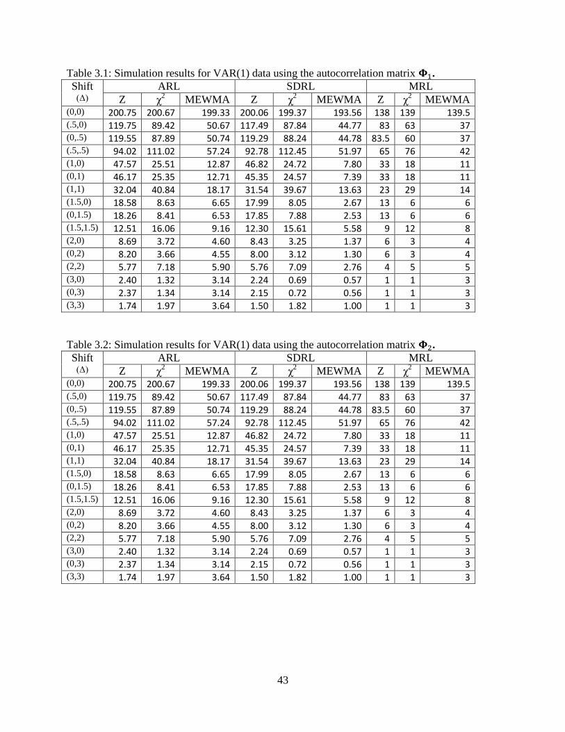
43

Table 3.1: Simulation results for VAR(1) data using the autocorrelation matrix .

Shift (Δ)

ARL SDRL MRL

Z χ2 MEWMA Z χ

2 MEWMA Z χ

2 MEWMA

(0,0) 200.75 200.67 199.33 200.06 199.37 193.56 138 139 139.5 (.5,0) 119.75 89.42 50.67 117.49 87.84 44.77 83 63 37 (0,.5) 119.55 87.89 50.74 119.29 88.24 44.78 83.5 60 37 (.5,.5) 94.02 111.02 57.24 92.78 112.45 51.97 65 76 42 (1,0) 47.57 25.51 12.87 46.82 24.72 7.80 33 18 11 (0,1) 46.17 25.35 12.71 45.35 24.57 7.39 33 18 11 (1,1) 32.04 40.84 18.17 31.54 39.67 13.63 23 29 14 (1.5,0) 18.58 8.63 6.65 17.99 8.05 2.67 13 6 6 (0,1.5) 18.26 8.41 6.53 17.85 7.88 2.53 13 6 6 (1.5,1.5) 12.51 16.06 9.16 12.30 15.61 5.58 9 12 8 (2,0) 8.69 3.72 4.60 8.43 3.25 1.37 6 3 4 (0,2) 8.20 3.66 4.55 8.00 3.12 1.30 6 3 4 (2,2) 5.77 7.18 5.90 5.76 7.09 2.76 4 5 5 (3,0) 2.40 1.32 3.14 2.24 0.69 0.57 1 1 3 (0,3) 2.37 1.34 3.14 2.15 0.72 0.56 1 1 3 (3,3) 1.74 1.97 3.64 1.50 1.82 1.00 1 1 3


Shift (Δ)

ARL SDRL MRL

Z χ2 MEWMA Z χ

2 MEWMA Z χ

2 MEWMA

(0,0) 200.75 200.67 199.33 200.06 199.37 193.56 138 139 139.5 (.5,0) 119.75 89.42 50.67 117.49 87.84 44.77 83 63 37 (0,.5) 119.55 87.89 50.74 119.29 88.24 44.78 83.5 60 37 (.5,.5) 94.02 111.02 57.24 92.78 112.45 51.97 65 76 42 (1,0) 47.57 25.51 12.87 46.82 24.72 7.80 33 18 11 (0,1) 46.17 25.35 12.71 45.35 24.57 7.39 33 18 11 (1,1) 32.04 40.84 18.17 31.54 39.67 13.63 23 29 14 (1.5,0) 18.58 8.63 6.65 17.99 8.05 2.67 13 6 6 (0,1.5) 18.26 8.41 6.53 17.85 7.88 2.53 13 6 6 (1.5,1.5) 12.51 16.06 9.16 12.30 15.61 5.58 9 12 8 (2,0) 8.69 3.72 4.60 8.43 3.25 1.37 6 3 4 (0,2) 8.20 3.66 4.55 8.00 3.12 1.30 6 3 4 (2,2) 5.77 7.18 5.90 5.76 7.09 2.76 4 5 5 (3,0) 2.40 1.32 3.14 2.24 0.69 0.57 1 1 3 (0,3) 2.37 1.34 3.14 2.15 0.72 0.56 1 1 3 (3,3) 1.74 1.97 3.64 1.50 1.82 1.00 1 1 3

44


Shift (Δ)

ARL SDRL MRL

Z χ2 MEWMA Z χ

2 MEWMA Z χ

2 MEWMA

(0,0) 200.75 200.67 199.33 200.06 199.37 193.56 138 139 139.5 (.5,0) 119.75 89.42 50.67 117.49 87.84 44.77 83 63 37 (0,.5) 119.55 87.89 50.74 119.29 88.24 44.78 83.5 60 37 (.5,.5) 94.02 111.02 57.24 92.78 112.45 51.97 65 76 42 (1,0) 47.57 25.51 12.87 46.82 24.72 7.80 33 18 11 (0,1) 46.17 25.35 12.71 45.35 24.57 7.39 33 18 11 (1,1) 32.04 40.84 18.17 31.54 39.67 13.63 23 29 14 (1.5,0) 18.58 8.63 6.65 17.99 8.05 2.67 13 6 6 (0,1.5) 18.26 8.41 6.53 17.85 7.88 2.53 13 6 6 (1.5,1.5) 12.51 16.06 9.16 12.30 15.61 5.58 9 12 8 (2,0) 8.69 3.72 4.60 8.43 3.25 1.37 6 3 4 (0,2) 8.20 3.66 4.55 8.00 3.12 1.30 6 3 4 (2,2) 5.77 7.18 5.90 5.76 7.09 2.76 4 5 5 (3,0) 2.40 1.32 3.14 2.24 0.69 0.57 1 1 3 (0,3) 2.37 1.34 3.14 2.15 0.72 0.56 1 1 3 (3,3) 1.74 1.97 3.64 1.50 1.82 1.00 1 1 3

3.3 Conclusions

As is well-known (see, e.g., Hayter and Tsui, 1994), there is no one control chart that

performs the best in all cases. Overall, all charts considered here are shown to have problems

detecting a mean shift when autocorrelation is present, even with the control limits set to achieve

a desired in-control ARL. The MEWMA detects a shift at least as quick as both the Z-chart and

the χ2 chart, except in the case of larger shifts ( ), which is expected since the parameter for

the MEWMA chart was chosen to detect small shifts. If a different value was chosen for the

parameter, the results may be different. The Z chart is able to detect a large shift in both variables

simultaneously quicker than the other charts and often detects small simultaneous shifts quicker

than the other charts. The other charts outperform the Z chart when there is a shift in only one

variable.

The Z chart‟s ability to detect shifts in both variables simultaneously may be due to a

certain “masking effect” of the positive correlation between the variables. When positive

45

correlation is present, as one variable increases, the other would also be expected to increase.

Since the Z chart considers the variables individually (using the correlation only to find the upper

control limit), this “masking effect” is not present. This is present, however, in most multivariate

control charts.

Aside from performance considerations, the Z chart appears to be preferable from a

practical point of view. This is mainly because of its diagnostic ability to determine which

variable or variables are actually out of control in case there is a signal by the chart. This is a

very useful feature that charts based on overall control statistics like the MEWMA do not have.

Some charts, like the MEWMA, also have the issue of choosing the appropriate charting

parameter(s), unlike the Z chart. Our study shows that the MEWMA and χ2 charts do not always

outperform the Z chart, so the diagnostic ability of the Z chart may encourage the practitioner to

use the Z chart whenever autocorrelation may be present.

To demonstrate the usefulness of the diagnostic ability of the Z chart, consider the

following example. Data were generated from a VAR(1) model with two parameters. A shift of

2σ was introduced to the second variable at time 0. The MEWMA chart and Z chart were applied

to the data. The charts can be seen below in Figures 3.1 and 3.2.

Figure 3.1: MEWMA chart applied to data.

Figure 3.2: Z chart applied to data.

46

As can be seen in Figures 3.1 and 3.2, the MEWMA chart detected the shift first at time

period 2 and the Z chart did not detect the shift until time period 4. The simulations showed that

this would often be the case. However, once the MEWMA chart signals, the process must be

investigated further to determine which variable or variables were at fault. With the Z chart, this

is not a problem. Since the Z chart plots the maximum of the statistics calculated at each time

period, the individual statistics are already calculated. Charts of the individual Z statistics can be

seen below in Figures 3.3 and 3.4.

Figure 3.3: Z statistic for first variable.

Figure 3.4: Z statistic for second variable.

Since the chart of the second variable shows the signal, we immediately know that the second

variable is out of control. Since the chart of the first variable does not show a signal, the first

variable can be viewed as still in control. Note that it is not necessary to create the individual

charts since it may be desired to see only the statistics at that time period and compare them to

the value of the upper control limit.

3.4 Future Work

More work needs to be done. For example, first, we considered only the case of having

two variables in our performance study. This should be extended to more than two variables. It

47

would also be of use to study the relationship between the autocorrelation coefficients and the

control limits of the Z chart, as well as other multivariate charts. The simulation procedure

works, but is very time-consuming and an easier method should be developed. This would make

the Z chart much more acceptable to practitioners since the control limits would be simpler to

calculate. Also, the parameters were assumed known. When these parameters are estimated, we

may observe different results. The assumption of multivariate normality of the data was also

appropriately met with our simulations. If this assumption is violated, the Z chart may not

perform as well. This should also be studied. The effect of the estimation of parameters and non-

normality are examined in Chapters 3 and 4, respectively.

48

CHAPTER 4

THE EFFECT OF PARAMETER ESTIMATION ON THE PERFORMANCE OF THE Z

CHART

4.1 Introduction

In many situations, the practitioner must estimate the parameters of the process to

construct the control chart to monitor the process. These parameters must be estimated from past

data and may not be accurate. There is evidence in the literature that control chart performance

degrades when estimated parameters are „plugged-in‟ and therefore there is a need to study the

effects of parameter estimation on the performance of other control charts.

In the case of estimated parameters, the charting statistic and thus the control limits are

random variables. Many authors derive the distribution of the charting statistic under estimated

parameters using various techniques including conditioning over the distribution of the estimated

parameters (see for example, Gibbons and Chakraborti, 2003). A common example of this is the

“Z” transformation. If the mean and standard deviation of a normal process are known, the

values could be „standardized,‟ i.e., subtracting the mean and dividing by the standard deviation

yielding values that follow a standard normal distribution. However, if the mean and standard

deviation are not known, subtracting the sample mean and dividing by the sample standard

deviation does not yield values following the standard normal distribution. In fact, it results in a

random variable following a t distribution, with a parameter called degrees of freedom that is

based on the size of the sample used for the estimation. Applying this idea to a control chart,

49

when the standardized charting statistic is used, the control limits say +/- 3 would only be

accurate when the parameters are known since the limits would be calculated based on the

standard normal distribution. The same chart, i.e., the standardized statistics and the +/-3 limits,

would lead to incorrect results (more false alarms, shorter in-control average run length) when

the parameters are estimated since appropriate percentiles of the t distribution should be used in

place of +/-3.

To demonstrate the effect of parameter estimation, consider the following. When the

process is in control, the charting statistic of the Z chart,

follows a standard normal distribution. If and are replaced with some suitable

estimates and , respectively, then the statistic becomes

which follows a t distribution with degrees of freedom, where n is the size of the sample

used to estimate the parameters. Noting this, as n increases, the distribution of the statistic

approaches the standard normal distribution, so that asymptotically the estimated parameters case

may be considered identical to the case of known parameters. However, it may be that in a

particular situation, the sample size is not large enough for these to be close. Therefore, for

“small” sample sizes, the chart may not achieve the desired in-control average run length when

the normal control limit is used.

Many researchers have studied the effects of parameter estimation on control chart

performance both in the univariate and the multivariate case. Some researchers use only

simulation studies to show the effect and others actually determine the distribution of the

50

charting statistic when estimated parameters are used. Adams and Tseng (1998) studied the

effect of parameter estimation on forecast-based monitoring schemes. They showed that control

charts applied to forecast residuals are very sensitive to errors in estimation and that the direction

of the error has an effect on the charts using estimated parameters. Kramer and Schmid (2000)

studied the effect on the ARL of univariate Shewhart-type charts including those using the

residuals of an autoregressive model. They show that when parameters are estimated, the

modified Shewhart chart, which uses modified control limits, is preferred since the traditional

charts are affected by known parameters. Champ et al. (2005) studied effects of estimation with

Hotelling‟s T2control chart. They show that when parameters are estimated, the control limits for

the known case are not appropriate. The in-control ARL is much higher with estimated

parameters and thus the chart is cannot detect shifts, especially small shifts, as quickly as when

the parameters are known. They also provide sample size recommendations to obtain a result that

is similar to the case of known parameters. Jensen et al. (2006) reviewed the literature on the

effect of the estimation of parameters on control chart properties, including charts for univariate,

multivariate, and autocorrelated data. Champ and Jones-Farmer (2007) also reviewed some

papers pertaining to the multivariate EWMA control chart and multivariate CUSUM control

charts. These works all show that parameter estimation has a serious effect on the performance of

control charts.

In this chapter, simulations will be performed to study the effects of parameter estimation

on the performance of the Z chart. Data will be generated from a vector autoregressive model.

The parameters required for the application of the Z chart will be estimated from a phase I

sample. The size of the sample will be varied to demonstrate the effect of the estimating sample

51

size on the performance of the Z chart. The Z chart with the estimated parameters will be applied

to simulated data. The effect on both the in-control and out-of-control run length will be studied.

4.2 Regression Approach to UCL Estimation

In practice, the alternative method of finding the upper control limit of the Z chart

described in Chapter 2 may not be very desirable since it requires an extensive binary search that

often requires a great amount of time. In order to facilitate the use of the Z chart in practice, the

UCL values were found for different parameters (matrix of autocorrelation parameters and error

covariance matrix) of bivariate VAR(1) models. A regression model was then fit to the UCL

values. Using only the cross-covariance of the two variables and the desired ARL, the model fits

the data with very little error, possibly due only to estimation. The regression model is

This yields an R2 value of 99.8%, showing a near perfect fit. When the desired ARL is 200, the

model is approximately

The regression model with the data can be seen below in Figure 4.1.

52

Figure 4.1: Predicting UCL for ARL0=200.

So, to use the Z chart, only the cross-covariance of the data, i.e., the covariance of the

process data, needs to be known. The cross-covariance of the two variables would be substituted

into the model and the UCL would be found. For example, if the cross-covariance between the

two variables is 1.44 and an ARL0 of 200 is desired, the UCL would then be

which simulations show yields an ARL0 of about 200, showing that the equation estimated the

UCL very well. Note that this model will only apply to bivariate data. Further work needs to be

done to find a theoretical derivation of the relationship and/or models for more than two

variables.

4.3 Estimation Procedures

For the estimation of the process mean vector, most practitioners would use the sample

mean vector given by

53

where is the ith

sample mean given by

, and is the observation of the

variable, with , where p is the number of variables and n is the sample size. The

sample mean vector is sensitive to outliers, so some practitioners may choose to use a trimmed

mean vector instead. The trimmed mean vector is found by „trimming‟ (removing) a chosen

percentage of observations from the lowest and highest regions of each variable of the data

matrix and calculating the sample mean vector of the remaining observations.

For the estimation of the cross-covariance matrix, many would simply use the unbiased

sample cross-covariance matrix given by

where is the vector of observations.

It may also be useful to consider the maximum likelihood approach. If the random

variable is normally distributed, the maximum likelihood estimator of the cross-covariance

matrix is defined as

which is not unbiased. For large sample sizes, the unbiased estimate S and the maximum

likelihood estimate Smle are approximately the same. When the sample size is small and the

number of parameters is large, the two previously-mentioned estimators are often unstable. To

handle this problem, shrinkage estimators have been proposed, such as in Shäfer and Strimmer

(2005). These estimators may provide estimators with a slightly better mean squared error than

the two others when the sample size is small and the number of parameters is large.

54

Robustness (or resistance) to outliers is an important issue in the estimation of the cross-

covariance matrix as well. The estimators mentioned above are not resistant to outliers. Other

methods exist that may be robust to outliers. An analysis of some of these can be seen in Vargas

(2003). One common method is to use trimmed data. Once the data is trimmed, the mean vector

and cross-covariance matrix can be computed and may be more accurate in the presence of

multiple outliers. Rousseeuw (1984) and Rousseeuw and van Zomeren (1990) created minimum

volume ellipsoid (MVE) estimators that use the smallest ellipsoid that contains at least half of the

observations. Rousseeuw and van Driessen (1999) proposed the minimum covariance

determinant (MCD) estimators which use an ellipsoid of the data whose covariance matrix has

the smallest determinant. Jensen, Birch, and Woodall (2007) study the use of the MVE and the

MCD as estimators for the cross-covariance matrix of the data. Vargas (2003) performed

simulation studies on these estimators and determines that all work well in the presence of

outliers. However, they also mention that these robust estimators may have a low probability in

detecting a shift in the mean vector, so they recommend simultaneously using both a chart that is

sensitive to sustained shifts and one that is robust to outliers.

In this chapter, we are assuming that no outliers are present and that the sample size is

larger than the number of variables (both by design). Also, since we would like to use the most

common estimators, the shrinkage estimators will be avoided. However, it may be beneficial to

use the aforementioned estimators in practice. Therefore, we will be using the sample mean

vector to estimate the mean vector µ and the unbiased sample cross-covariance matrix to

estimate the cross-covariance matrix .

55

4.4 Simulation

To compare the known parameters case with the case of estimated parameters, charts for

both cases will be constructed. The sample size used to estimate the necessary parameters to

build the chart will be varied so that the effect of sample size can be seen. Both the cross-

covariance and the mean of the data need to be estimated.

Data is generated from a VAR(1) model with the following parameters:

First, the in-control performance is studied. To do this, the UCL will be set to obtain a desired in-

control ARL (ARL0) when the parameters are known. Then, using the UCL that enables the chart

to obtain a desired ARL0 in the known parameters case, the ARL0 of the estimated parameters

case is found.

For the in-control study, the estimation procedure is as follows:

1) Generate n values from the VAR(1) model above.

2) Calculate the sample mean and sample cross-covariance matrix of the data.

3) Using the UCL from the known case, apply the Z chart and determine the run length

of the process.

4) Repeat 1-3 a large number of times (say 10,000, yielding a result within about 0.003

of the true value).

The in-control results can be seen below in Table 4.1. The table shows the in-control

ARL, standard deviation of the run length (SDRL), median run length (MRL), and the 5th

, 25th

,

75th

, and 95th

percentiles of the run length.

56

Table 4.1: In-control results.

Case ARL SRL 5th

Pct

25th

Pct

MRL 75th

Pct

95th

Pct

Known 200.750 200.060 12 23 138 461 614

Estimated with 452.801 8498.688 5 18 48 130 805

Estimated with 319.567 2891.264 7 24 64 170 859

Estimated with 290.072 2692.318 8 29 76 196 908

Estimated with 219.415 503.765 9 36 92 216 794

Estimated with 224.174 552.892 10 41 100 235 755

Estimated with 215.282 428.869 11 43 107 239 746

Estimated with 205.292 278.901 12 50 119 255.25 680

Estimated with 206.237 251.611 13 53 125 265 667

Estimated with 200.071 220.799 14 55 129 263 627

The in-control results for the ARL0, SDRL, and MRL are shown graphically in Figures

4.2-4.4 below. Reference lines have been added to show the ARL0, SDRL, and MRL

approaching that of the known parameters case.

Figure 4.2: ARL0 for different estimating

sample sizes.

Figure 4.3: SDRL for different estimating

sample sizes.

57

Figure 4.4: MRL for different estimating sample sizes.

In application of the chart, the model presented earlier,

may be used. To examine the effect of the estimation on the ARL0 of the chart using this model,

the following procedure was used:

1) Generate a sample of size n from the VAR(1) model with above.

2) Calculate the sample mean and sample cross-covariance matrix of the data.

3) Calculate the UCL from the equation above.

4) Simulate the run length.

5) Repeat 1-3 a large number of times (say 10,000, yielding a value of about 0.003 of the

actual value).

Both the in-control and out-of-control results can be seen below in Table 4.2.

58

Table 4.2: Out-of-control results. Known Estimated with Estimated with

Δ ARL SRL MRL ARL SRL MRL ARL SRL MRL

(0,0) 200.60 197.01 140 167.83 594.33 56 168.92 399.10 69 (.5,0) 133.56 127.84 95 103.60 277.64 41 121.32 310.89 51 (0,.5) 130.83 126.47 93 99.18 246.93 38 109.66 206.05 51 (.5,.5) 119.44 114.66 85 90.45 316.72 39 100.86 208.65 47 (1,0) 62.23 61.93 43 51.81 204.25 22 52.83 87.79 26 (0,1) 56.52 55.74 39 43.98 107.57 20 49.98 79.79 26 (1,1) 49.92 49.04 35 36.53 61.16 18 40.26 59.35 22 (1.5,0) 29.18 28.53 20 20.89 34.53 10 23.76 34.07 13 (0,1.5) 26.19 25.77 18 19.09 33.93 10 22.12 32.03 12 (1.5,1.5) 22.28 22.90 14 15.53 24.73 7 17.90 25.32 9 (2,0) 13.15 14.02 8 9.54 16.96 4 10.78 15.78 5 (0,2) 12.25 13.33 7 9.06 14.48 4 10.23 15.32 5 (2,2) 9.87 11.57 5 6.58 11.30 2 7.82 12.00 3 (3,0) 2.34 3.18 1 2.08 3.77 1 2.16 3.78 1 (0,3) 2.38 3.16 1 2.05 3.34 1 2.13 3.30 1 (3,3) 1.68 2.29 1 1.48 2.26 1 1.54 2.21 1

Estimated with Estimated with Estimated with


(0,0) 181.64 334.65 82 187.47 295.08 100 190.58 270.08 107 (.5,0) 121.91 231.44 59 124.04 184.72 66 126.94 174.81 72 (0,.5) 118.10 220.23 59 125.16 192.86 68 125.55 165.32 72 (.5,.5) 104.60 159.41 53 108.85 144.89 61 111.08 140.13 66 (1,0) 54.93 84.48 30 55.76 78.85 33 58.38 74.93 36 (0,1) 51.61 78.61 28 52.64 65.17 31 55.34 67.71 34 (1,1) 43.64 61.42 24 44.69 54.06 27 45.61 52.30 28 (1.5,0) 24.85 34.12 14 26.24 31.54 16 26.85 31.51 17 (0,1.5) 23.94 31.93 13 23.73 29.09 14 24.33 27.86 15 (1.5,1.5) 19.05 24.97 10 19.23 23.45 11 20.16 23.45 12 (2,0) 11.44 15.85 6 11.89 15.00 6 12.58 15.74 7 (0,2) 10.33 13.92 5 11.04 14.04 6 11.35 14.06 6 (2,2) 8.03 11.76 3 8.53 11.39 4 9.01 11.67 4 (3,0) 2.23 3.47 1 2.35 4.00 1 2.34 3.70 1 (0,3) 2.27 3.49 1 2.20 3.14 1 2.32 3.35 1 (3,3) 1.55 2.12 1 1.62 2.35 1 1.67 2.48 1

59

Estimated with Estimated with Estimated with


(0,0) 190.21 244.47 110 195.21 220.96 123 197.82 219.13 127 (.5,0) 126.46 162.93 77 130.91 145.00 86 131.60 146.01 86 (0,.5) 125.04 162.88 75 123.72 135.09 81 127.92 134.34 85 (.5,.5) 114.93 146.85 67 115.66 126.11 75 115.68 123.00 77 (1,0) 58.88 67.37 38 60.88 63.61 40 59.77 62.05 40 (0,1) 54.82 61.33 35 56.36 60.42 37 57.42 60.40 39 (1,1) 46.56 53.39 29.5 47.31 49.16 32 48.63 50.08 32 (1.5,0) 26.92 30.94 17 27.82 29.28 19 27.73 28.46 18 (0,1.5) 25.08 28.61 16 25.60 27.56 17 25.82 26.67 17 (1.5,1.5) 20.42 23.31 12 21.74 23.27 14 21.46 22.82 14 (2,0) 12.38 14.79 7 13.14 15.22 8 13.05 14.69 8 (0,2) 11.67 13.92 6 11.86 13.61 7 11.81 13.27 7 (2,2) 8.99 11.56 4 9.39 11.55 5 9.55 11.44 5 (3,0) 2.36 3.63 1 2.42 3.60 1 2.41 3.59 1 (0,3) 2.36 3.38 1 2.34 3.31 1 2.39 3.34 1 (3,3) 1.62 2.19 1 1.72 2.37 1 1.71 2.34 1

Estimated with

Δ ARL SRL MRL

(0,0) 195.52 208.75 129 (.5,0) 138.22 146.39 90 (0,.5) 125.36 128.06 85 (.5,.5) 117.40 123.17 79 (1,0) 61.00 61.70 41 (0,1) 56.55 56.43 39 (1,1) 48.44 50.77 33 (1.5,0) 28.03 28.14 19 (0,1.5) 26.01 26.57 17 (1.5,1.5) 21.78 23.52 14 (2,0) 13.33 14.69 8 (0,2) 12.26 13.72 7 (2,2) 9.58 11.56 5 (3,0) 2.35 3.34 1 (0,3) 2.34 3.14 1 (3,3) 1.70 2.32 1

60

4.5 Results and Conclusions

As expected, when the mean vector and cross-covariance matrix of the process are

estimated, the desired ARL0 is not achieved. As the estimating (phase I) sample size increases,

the attained ARL0 approaches the desired ARL0. It is also important to note that as the sample

size increases, the variability of the estimators decreases and thus the standard deviation of the

run length decreases. Specifically, for small sample sizes (less than about 100 vectors), the

attained ARL0 and MRL is much less than the desired, and with such a high variability of the

estimates, it is difficult to obtain the desired ARL0.

The tables presented in this paper provide a means both for determining the necessary

sample size to accurately estimate the parameters for the Z chart and to determine the error of the

estimation when only a certain sample size is available. For example, suppose that the

practitioner needs to have an idea of a sample size in phase I to have and ARL0 of no less than

190 (on average). He would then choose a sample of at least size 200 (if possible) to obtain that

value. Also, he may understand that the standard deviation of the run length will be about 270

(on average). Another example involves the latter use of the charts. Consider a practitioner

having a phase I sample of 100 observation vectors who would like to use the Z chart. She could

then understand that the ARL0 will be approximately 182 (on average) and the standard deviation

of the run length of 335 (on average). This would lead to a more accurate interpretation of a

signal.

Although it may seem that a large phase I sample size is recommended to achieve the

desired results, it is comparative to the phase I sample sizes for other multivariate charts and

charts for autocorrelated data. Adams and Tseng (1998) suggested a phase I sample of at least

200 observations to use residuals control charts on individual observations. Nedumaran and

61

Pignatiello (1999) recommended a phase I sample of at least 200 observations (with samples of

size 5) in using Hotelling‟s T2 charts. Therefore, needing a phase I sample of at least, say 200, for

the use of the Z chart may not be of much concern in comparison to the size required for other

charts.

62

CHAPTER 5

THE ROBUSTNESS OF THE Z CHART TO THE ASSUMPTION OF MULTIVARIATE

NORMALITY

5.1 Introduction

In many situations the necessary distributional assumption for a control chart may not be

justified. This may be due to the data obviously not following the necessary distribution or

simply that not enough information is available to check if the process follows the assumed

distribution. Akkaya and Tiku (2001) mention that “non-normal distributions are more prevalent

in practice.” It may be that the control chart has been constructed under the assumption of a

normal distribution and yet there is not convincing evidence that the normal distribution is a

good model for the data distribution in the application at hand. A distributional assumption is

necessary in the implementation and application of many charts. For example, an individuals

control chart requires the normality assumption to be valid. If the distributional assumption

cannot be justified, the probability distribution of the charting statistic would be affected, at least

for small to moderate sample sizes, and hence the original control limits may not be appropriate.

This could seriously affect the performance of the control chart both in terms of the number of

false alarms (way too many or few) and the shift detection capability.

This practical concern leads to studying the issue of robustness of control charts to the

assumption of the distribution. This has been a topic studied by many researchers, both in the

univariate and multivariate cases. Schilling and Nelson (1976) were among the first to study the

effect of non-normality on control charts. Yourstone and Zimmer (1992) developed a non-

63

symmetric control chart for averages to be applied to non-normal data. Willemain and Runger

(1996) proposed using the empirical percentiles of the data distribution to determine the control

limits for the individuals chart when the data are not normal. Borror, Montgomery, and Runger

(1999) showed that the individuals chart and the EWMA chart are affected when the assumption

of normality is violated. They also showed that the EWMA chart may be designed (charting

constant can be fine tuned) so that it is robust to the normality assumption. However, recent work

by Human et al. (2009) showed that even the most robust EWMA chart obtained this way can

still be significantly affected by the presence of contaminated data, so there is need for caution.

In the multivariate case, Stoumbos and Sullivan (2002) studied the effects of non-normality on

the MEWMA and the T2 chart. They also showed that the charting parameter of the MEWMA

may be adjusted to handle non-normal situations. However, this is bound to be tedious and

inefficient. In many potential applications, the sample size is assumed to be large enough to

assume that the sample mean vector is approximately (univariate/multivariate) normal by the

central limit theorem. However, this assumption is often questionable with smaller sample sizes,

especially for individuals charts. Chou, Mason, and Young (2001) studied the effect of

multivariate non-normality on the T2 chart. They note that the phase II UCL for the chart based

on the F distribution may be very inaccurate. They used a kernel smoothing technique to estimate

the distribution of the T2 statistic so that a more accurate UCL could be created. They also

developed a sample size requirement for data taken from a multivariate exponential distribution.

Most autoregressive models, both univariate and multivariate, require the assumption of

normality (or multivariate normality). In this chapter, both the in-control and out-of-control

performance of the Z chart will be studied when the error distribution is not multivariate normal.

Different parameters of the multivariate t and multivariate gamma distributions will be

64

considered. A description of the multivariate t and multivariate gamma distributions can be

found in Appendices A and B.

5.2 Simulation

The in-control and out-of-control ARL will be studied. All parameters are assumed

known. Data are generated from a VAR(1) model with

The error covariance matrix that will be used is

Note that the covariance matrix is the actual covariance matrix for the multivariate normal

distribution. The other two distributions will have transformations of the covariance matrix as the

covariance matrix for the specific case.

To obtain the error covariance matrix Σ when the data follow a multivariate t distribution,

the following equation must be solved:

where and are the parameters of the multivariate t distribution. Solving for the

parameter, the equation becomes

So, to achieve the desired error covariance matrix Σ, the following values for the multivariate t

parameter were used:

65

The scale parameter for the multivariate gamma distributions will be set to 1 so that only the

skewness of the distribution will be adjusted. To obtain the error covariance matrix Σ when the

data follow a multivariate gamma distribution, the following equation must be solved:

where is the ijth

element of the target covariance matrix, is the ijth

element of the

parameter of the Wishart distribution, and is the shape parameter of the multivariate gamma

distribution. Solving for the ijth

element of the Wishart parameter , the equation becomes

So, to achieve the desired error covariance matrix Σ, the following values for the Wishart

parameter were used:

Also note that the mean of the random values from the multivariate gamma distribution is related

to the matrix. To ensure that the mean of the error terms is the zero vector, the mean will

be subtracted from the generated observations.

Since the error covariance matrix and the matrix of autocorrelation parameters are

constant for every case, the cross-covariance matrix of the process is

66

In order to obtain an in-control ARL of 200, the upper control limit was found to be 2.781. Note

that since the process covariance matrix is the same for each case, the upper control limit also

does not change.

The results of the simulation can be seen below in Table 5.1. The table shows the average

run length, standard deviation of the run length, and the 5th

, 25th

, 50th

, 75th

, and 95th

percentiles of

the run length.

Table 5.1: In-control run length of the Z chart for various distributions using UCL=2.781.

Distribution ARL SDRL 5th

25th

MRL 75th

95th

MVN 200.60 197.01 15 61 140 274 595

MVT(3) 109.55 107.78 7 22 51 99 212

MVT(5) 121.36 120.82 9 36 84 165 365

MVT(7) 139.41 137.50 10 42 97 192 416

MVT(10) 157.98 155.58 11 47 111 217 476

MVT(20) 177.33 174.98 13 54 123 245 524

MVG(2) 103.94 103.68 7 30 72 145 306

MVG(4) 130.09 127.66 8 38 91 179 384

MVG(8) 157.12 155.61 10 46 108 217 471

MVG(16) 177.85 178.07 12 52 122 243 533

MVG(64) 195.19 190.58 14 57 137 270 585

It can be seen that for data that are far from multivariate normal, the ARL0 is far from the

desired ARL0 of 200. As the distribution approaches multivariate normality, the ARL0

approaches the desired ARL0 of 200.

To observe the performance of the Z chart in practice, shifts were introduced to the

process. Both the in-control and out-of-control results can be seen below in Table 5.2. Note that

the ARL for the shifts may be slightly misleading in comparing each case since the in-control

ARL is not equal in each of the cases. However, in practice it may be the case where the control

limit is found under the assumption of normality, so it is important to understand the out-of-

control performance of the chart when the attained in-control ARL is not the same as the desired.

67

Table 5.2: Out-of-control results. MVN MVT(3) MVT(5)

Δ ARL SDRL MRL ARL SDRL MRL ARL SDRL MRL

(0,0) 200.60 197.01 140 109.55 107.78 77 121.36 120.82 84 (.5,0) 133.56 127.84 95 71.55 69.21 51 64.00 61.82 45 (0,.5) 130.83 126.47 93 72.56 71.36 52 68.03 65.49 48 (.5,.5) 119.44 114.66 85 64.56 64.19 44 58.50 58.16 41 (1,0) 62.23 61.93 43 22.79 22.68 16 19.17 19.35 13 (0,1) 56.52 55.74 39 27.64 27.53 19 22.98 22.79 16 (1,1) 49.92 49.04 35 20.82 21.40 14 17.02 18.18 11 (1.5,0) 29.18 28.53 20 4.37 6.02 2 4.21 5.72 2 (0,1.5) 26.19 25.77 18 7.45 8.78 4 6.43 7.64 3 (1.5,1.5) 22.28 22.90 14 3.73 5.17 2 3.51 5.00 1 (2,0) 13.15 14.02 8 1.12 0.83 1 1.13 0.83 1 (0,2) 12.25 13.33 7 1.39 1.58 1 1.55 1.78 1 (2,2) 9.87 11.57 5 1.08 0.67 1 1.08 0.65 1 (3,0) 2.34 3.18 1 1.00 0.04 1 1.00 0.04 1 (0,3) 2.38 3.16 1 1.01 0.12 1 1.01 0.09 1 (3,3) 1.68 2.29 1 1.00 0.08 1 1.00 0.07 1

MVT(10) MVT(20) MVG(2)


(0,0) 157.98 155.58 111 177.33 174.98 123 103.94 103.68 72 (.5,0) 68.81 64.90 49 70.70 69.02 49 51.66 51.45 36 (0,.5) 72.41 69.37 51 74.91 72.10 53 51.74 52.18 35 (.5,.5) 59.60 58.40 41 61.66 61.04 42 37.87 38.13 26 (1,0) 18.11 18.39 12 18.03 18.72 12 19.69 20.88 13 (0,1) 22.19 22.27 15 21.73 21.48 15 21.88 22.84 14 (1,1) 15.92 17.29 10 15.79 17.09 10 14.50 16.00 9 (1.5,0) 4.04 5.39 2 4.10 5.50 2 5.65 7.23 3 (0,1.5) 6.16 7.57 3 6.01 7.24 3 7.80 9.23 4 (1.5,1.5) 3.51 5.18 1 3.33 4.81 1 4.42 5.81 2 (2,0) 1.14 0.80 1 1.16 0.87 1 1.00 0.00 1 (0,2) 1.63 1.90 1 1.62 1.82 1 1.70 2.33 1 (2,2) 1.11 0.79 1 1.10 0.71 1 1.00 0.00 1 (3,0) 1.00 0.01 1 1.00 0.01 1 1.00 0.00 1 (0,3) 1.00 0.08 1 1.00 0.04 1 1.00 0.00 1 (3,3) 1.00 0.00 1 1.00 0.00 1 1.00 0.00 1

68

MVG(4) MVG(8) MVG(16)


(0,0) 130.09 127.66 91 157.12 155.61 108 177.85 178.07 122 (.5,0) 57.14 56.95 40 61.53 60.91 43 64.61 62.46 45 (0,.5) 57.81 58.44 40 63.27 61.74 44 66.27 64.65 47 (.5,.5) 42.32 42.21 29 45.83 45.93 32 50.75 50.65 35 (1,0) 19.12 20.18 12 18.49 19.66 12 18.67 19.87 12 (0,1) 21.01 21.99 14 21.52 22.37 14 21.53 22.33 14 (1,1) 14.44 15.85 9 14.77 16.31 9 14.83 16.41 9 (1.5,0) 5.28 7.10 2 4.84 6.49 2 4.70 6.43 2 (0,1.5) 7.33 8.82 4 7.01 8.55 4 6.56 7.85 3 (1.5,1.5) 4.03 5.50 2 3.80 5.21 2 3.62 5.01 1 (2,0) 1.00 0.00 1 1.05 0.54 1 1.09 0.64 1 (0,2) 1.75 2.24 1 1.79 2.32 1 1.73 2.12 1 (2,2) 1.00 0.00 1 1.02 0.35 1 1.05 0.54 1 (3,0) 1.00 0.00 1 1.00 0.00 1 1.00 0.00 1 (0,3) 1.00 0.00 1 1.00 0.00 1 1.00 0.00 1 (3,3) 1.00 0.00 1 1.00 0.00 1 1.00 0.00 1

From the simulations, we can see that when the distribution is far from normal, many

more false alarms are present. When the distribution is diagonally symmetric but not multivariate

normal, as in the case of the multivariate t distribution, the performance seems to very similar to

the case when the distribution is not diagonally symmetric. However, when the distribution is not

far from normal, the run length and detection ability is similar to that of the normal distribution.

5.3 Results and Conclusions

As expected, the simulations show that the performance of the Z chart deteriorates for

process data that do not follow a multivariate normal distribution. If the practitioner has reasons

to believe that the data are not far from the normal, it still may be acceptable to use the chart.

However, this belief has to be well justified or there can be serious consequences. For example,

consider univariate t data. One-thousand values were generated from a t distribution with 5

degrees of freedom and a normal probability plot was constructed. The plot can be seen below in

Figure 5.1.

69

Figure 5.1: Normal probability plot of t(5) data.

Some practitioners may feel that from the normal probability plot, the data are from a

normal distribution. Not only do most of the points lay along the line, the Anderson-Darling test

yields p-value greater than the often-desired value of 0.05. However, the simulations have shown

that when the data is multivariate t with 5 degrees of freedom, the performance of the Z chart is

far from what is expected or desired.

This chapter, as well as other papers in the literature exploring the robustness of various

multivariate control charts to non-normality, have shown that these charts are very sensitive to

the normality assumption and their in-control performance is substantially degraded in the

absence of normality. It is often the case in practice that the data are not normal or there is not

enough evidence to determine that the data may be considered normal. Therefore, it seems

reasonable to conclude that more work should be done to develop distribution-free techniques for

these situations.

t(5)

Pe

rce

nt

43210-1-2-3-4

99.9

99

95

90

80

7060504030

20

10

5

1

0.1

Mean

0.081

0.05048

StDev 1.035

N 100

AD 0.664

P-Value

Normal Probability Plot of t(5) DataNormal

70

CHAPTER 6

SOME SIMPLE MULTIVARIATE NONPARAMETRIC CONTROL CHARTS

6.1 Introduction

It has been noted that (e.g. Woodall and Montgomery, 1999) that the control charting

methodology shares similarities with classical statistical inference methods such as hypothesis

testing and confidence intervals. Many statistical inference procedures are derived under the

assumption that the variable(s) under study follows some specific parametric distribution. These

are called parametric inference procedures. However, the reality is that such information is

seldom, if ever, available to the practitioner trying to solve the problem. When the parametric

assumption may be violated, these parametric tests may not be valid. It has been noted that these

parametric tests are “exactly valid only so long as the assumptions themselves can be

substantiated” (Gibbons and Chakraborti, 2003). To overcome this issue, statistical inference

procedures, including hypothesis tests, confidence intervals and control charts that do not require

making any specific parametric distributional assumptions have been proposed and studied.

Collectively, these techniques are called nonparametric or distribution-free techniques.

This situation also applies to control charts. When the distributional assumptions

underlying a parametric control chart are violated, the performance of the control chart often

deteriorates both in terms of the false alarm rate and the power of detection. Thus, in a situation

like this, a nonparametric control chart may prove to be a better alternative. It is worth noting

that an argument often made against the use of nonparametric control charts, as well as using

71

nonparametric statistical inference (hypothesis tests, confidence intervals), is that the power of

the chart (or test) is not as high as the power of a parametric chart (or test). This is of course true

when the distributional assumptions for the parametric chart are exactly satisfied. However, as

we said before, in practice it is rare to expect that the distributional assumptions will be exactly

met, or verified, or in fact that such information will be available to the practitioner.

Several nonparametric univariate control charts have been developed in the literature. An

overview of many of these charts was presented by Chakraborti, van der Laan, and Bakir (2001)

and more recently in Chakraborti and Graham (2008). For example, Bakir and Reynolds (1979)

considered a cumulative sum chart base on the Wilcoxon signed-rank statistic. Bakir (2004)

considered a Shewhart-type chart based on the Wilcoxon signed-rank statistic as well. Runger

and Willemain (1995) created charts that are model-free and were created to cope with

autocorrelated data. These include a weighted batch means control chart and an unweighted

batch means control chart. Albers and Kallenberg (2006) created a MIN chart that is

nonparametric and uses the subgroup minima instead of the average of the subgroup. Chakraborti

and Eryilmaz (2007) developed an effective enhancement of this chart by incorporating some

“runs” type signaling rules. Chakraborti and van de Wiel (2008) developed a nonparametric

control chart based on the Mann-Whitney statistic. Graham et al. (2009) and Jones-Farmer,

Jordan, and Champ (2009) have considered distribution-free phase I control charts. Chatterjee

and Qiu (2009) developed a class of distribution-free CUSUM charts, using bootstrapping to find

the control limits. Balakrishnan, Triantafyllou, and Koutras (2009) proposed nonparametric

control charts using runs and Wilcoxon rank sum statistics. Zou, Qiu, and Hawkins (2009)

developed a nonparametric chart for profiles using change point formulation.

72

Parametric multivariate inference techniques, just as their univariate counterparts, rely on

certain distributional assumptions. As in the univariate case, if these assumptions cannot be

properly justified, or are not true, the results and the conclusions of the corresponding inference

procedures may not be valid. In the quality control setting, this could lead to an excessive

number of false alarms, for example, which will reduce the effectiveness of the monitoring

strategy. With this motivation, some multivariate nonparametric techniques have been

developed in the literature. Two of the more popular ones are the multivariate Wilcoxon signed-

rank test and the multivariate sign test. The critical values for these tests may be obtained using

the asymptotic distribution or by simulation. An overview of some multivariate nonparametric

tests can be found in Oja and Randles (2004).

As in the univariate case, multivariate nonparametric tests can be adapted to propose

multivariate control charts. When the multivariate distribution assumption of a multivariate

control chart is violated or unjustifiable, the signals and the conclusions from the parametric

chart become questionable. Nonparametric multivariate control charts can provide better

alternatives in such situations. Although several nonparametric control charts have been

introduced for use with univariate data, relatively few, simple to use, nonparametric control

charts currently exist for multivariate data. Das (2009) recently proposed a nonparametric

Shewhart-type control chart based on the sign test considered by Puri and Sen (1971). However,

only the case of two variables (bivariate) was considered. Qiu and Hawkins (2001) developed a

nonparametric multivariate cumulative sum control chart based on the antirank vector of the

observations. The antirank vector is the vector of the indices of the order statistics. A

multivariate CUSUM procedure is then applied to monitor changes in the process. The procedure

73

is computationally intensive but is shown to be very effective in non-normal situations. The

authors also state that using the antiranks is particularly useful in detecting a downward shift.

Kapatou and Reynolds (1994, 1998) developed multivariate nonparametric control charts

for small samples and studied charts for cases when the covariance matrix of the observations is

assumed known. Liu (1995) developed a series of multivariate nonparametric control charts

based on the concept of data depth, proposed by Liu (1990). The idea is to “reduce” the

multivariate measurements to some univariate indices using the concept of data depth, given a

statistic calculated to determine how close the points are to the center of the data set. Based on

this statistic, charts similar to the X chart for individuals, the chart, and the CUSUM chart can

be created. Liu, Singh and Teng (2004) extended this idea to include a moving average

nonparametric multivariate control chart that improves on the detection ability of Liu‟s earlier

charts. They perform a comparison with Hotelling‟s T2 chart and conclude that the ability to

detect an out-of-control situation is similar in the case of a multivariate normal distribution

except for very small shifts. However, when the multivariate normal assumption is violated, their

chart outperforms other charts since their chart is distribution-free. Continuing along this idea of

using the depth concept, Hamurkaroglu, Mert and Saykan (2004) developed nonparametric

control charts based on the Mahalanobis depth. Although the list of developed nonparametric

multivariate control charts is short, it has become a popular topic as of late.

Four nonparametric multivariate control charts are proposed and studied here first. All

are Shewhart-type charts to be used with independent and identically distributed samples arising

from some multivariate symmetric distribution (also called diagonally symmetric). This

generalizes the application to more than the multivariate normal distribution. The main

advantage of a Shewhart-type chart is its simplicity in calculation and application and in the

74

multivariate setting, as noted by Mason and Young (2002), simplicity may be a crucial virtue

from a practical point of view. The first proposed chart is based on the multivariate form of the

sign test considered by Puri and Sen (1976) and the second chart is based on the Wilcoxon

signed-rank statistic described in Hettmansperger (2006). Next, we consider two multiple

comparisons type charts based on the maximum of multiple univariate sign and Wilcoxon

signed-rank statistics. The last two charts can be viewed as nonparametric analogs of Hayter and

Tsui‟s (1994) M chart and Kalgonda and Kulkarni‟s (2004) Z chart. Both the Shewhart-type and

multiple comparisons-type charts are expected to be efficient in detecting larger shifts in the

mean (location) and are simple to use. The multiple comparisons-type control charts also have a

practical advantage in that they have the diagnostic ability to immediately determine which

variable or variables contributed to a signal. Applications to independent samples of data will be

considered. The performance of the control charts, along with sample size requirements, will be

studied in comparison with Hotelling‟s χ2 chart.

6.2 Shewhart-Type Charts

We first consider a Shewhart-type chart based on the multivariate version of the sign test.

No assumptions about the underlying distributions are required except that they are continuous

and that their corresponding location parameters (medians, for example) are uniquely defined.

6.2.1 The Multivariate Sign Control Chart

The usual sign test is a simple yet versatile univariate nonparametric test (see Gibbons

and Chakraborti, 2003). The multivariate sign control chart is based on the multivariate form of

the sign test (see e.g. in Hettmansperger, 2006). This will be referred to as the chart.

75

Suppose that we need to monitor the in-control medians of p

variables, where the in-control medians are assumed known. For each of the p

variables, compute the univariate sign statistic

where for the ith

variable is the jth

observation, n is the total number of observations, is

the specified in-control value of the median and

Thus, Let S be the px1 vector of the ‟s. It is

known that (see Hettmansperger, 2006) is asymptotically distributed as multivariate

normal with mean vector 0 and a covariance matrix which can be consistently estimated by

defined as

The multivariate sign charting statistic is then

For large sample sizes, the limiting distribution of the statistic is χ2 with p degrees of

freedom. It is important to note here that the proposed multivariate sign test (as well as the

chart) is distribution-free for large sample sizes (asymptotically distribution-free) and in practice,

the chi-squared distribution is used to define the control limit. For a given nominal false alarm

76

rate of α, the proposed chart has a lower control limit of zero and an upper control limit of

It may be noted that when , that is when there are two variables, the statistic

simplifies to a form given in Puri and Sen (1976) (also see Hettmansperger, 2006). Das (2009)

used this to consider a control chart in the bivariate case. The proposed chart is an extension of

this chart to the case of more than two variables. Further note that although we assumed the

location parameters to be the medians, the sign procedure and hence the control chart can apply

equally well for other percentiles.

While the sign chart (test) is the simplest nonparametric chart (test) that can be used in

practice, it is well known in the univariate case that a more powerful testing procedure can

sometimes be obtained when the underlying distribution is symmetric, based on the so-called

signed-ranks. Along these lines, in the multivariate case we consider the multivariate Wilcoxon

signed-rank control chart.

6.2.2 The Multivariate Wilcoxon Signed-Rank Control Chart

The multivariate Wilcoxon signed-rank control chart proposed here is based on the

multivariate form of the Wilcoxon signed-rank test, as defined by Hettmansperger (2006). This

will be referred to as the chart. Again suppose that the in-control values of the medians are

specified as before. However, now assume further that the joint distribution of the p variables is

diagonally symmetric about Under this assumption, it follows that the

marginal distributions of the individual variables are symmetric about their respective medians.

In the in-control situation, where is the specified value of the

median of the ith

variable.

77

For each of the p variables, compute the univariate Wilcoxon signed-rank statistic

where is the rank of among ,…, Let W be the

px1 vector of the ‟s. It has been shown (see Hettmansperger, 2006) that the asymptotic

distribution of is multivariate normal with mean vector 0 and a covariance matrix

which can be consistently estimated with where is defined as

The multivariate signed-rank charting statistic is then

The limiting distribution of the statistic is χ2 with p degrees of freedom. Note here

that the medians are specified when the process is in-control. The asymptotic covariance matrix,

however, is not. Thus the consistent estimator of the asymptotic covariance matrix is used and

is calculated at each point in time when the charting statistic is calculated and plotted. Note again

that similar to the multivariate sign test, the multivariate Wilcoxon test (as well as the chart)

is not distribution-free for finite samples. The chi-squared approximation is used here as well.

For construction of the control chart with a given false alarm rate of α, the lower control limit is

zero with an upper control limit of

78

6.3 Charts Based on the Maximum of Multiple Univariate Nonparametric Statistics

Even though the Shewhart-type charts are easy to use and can detect moderate to large

shifts in the medians, a practical issue with these “overall” charts is the post-signal diagnosis,

that is, locating the source(s) that is(are) responsible for the shift. A control chart based on the

idea of multiple comparisons has the advantage that they can point to the origin of the as soon as

the overall control statistic signals. Hayter and Tsui (1994) considered such charts and concluded

that they are reasonably powerful (no chart is always the best). Motivated by their observations,

we consider certain nonparametric multiple comparisons type charts which can be viewed as

nonparametric analogs of their M chart and Kalgonda and Kulkarni‟s (2004) Z chart.

6.3.1 The Maximum Sign Chart

Following the M and Z charts, our proposal is to monitor the process at each time point

using the maximum of the absolute value of the standardized sign statistic, In

order to find the control limits for the proposed chart, the in-control distribution of the charting

statistic is needed. Note that as shown earlier, the asymptotic distribution of is normal

with mean 0 and a consistent estimator of the asymptotic variance is . This implies that the

asymptotic in-control distribution of is normal with mean 0 and the consistent estimator of the

asymptotic variance is .

To compare the values of the statistics, each should be standardized. The standardized

sign statistics are

The proposed charting statistic is the maximum of the standardized statistics

79

Asymptotically, the marginal distribution of each statistic, , for each variable, is

standard normal. However, the distribution of is dependent not only on the distribution of the

individual statistics, but the correlations among these statistics as well. These correlations must

be either assumed known or estimated from some data in order to implement the control chart.

Simulations show that the correlations of the ‟s are the same as of the correlation of the

process data. For example, if the correlation between two variables is 0.6, the correlation of the

sign statistics for each would be 0.4. Since the correlations must be known, the multiple-

comparisons-type multivariate nonparametric control charts considered here are not fully

nonparametric.

It may be noted that unlike the parametric charts, for nonparametric charts (both

Shewhart and multiple comparison type charts) some nominal values of the false alarm rate may

not be attainable for „small‟ sample sizes, without some form of randomization (see for example

Gibbons and Chakraborti, 2003). This is typical with most nonparametric tests and control charts

and is due to the fact that the charting statistic (here the sign statistic) has a discrete distribution.

For example, if the sample size is 5, the only choices for a false alarm rate are 0.0312, 0.1875,

and 0.5000 for one-sided tests and each divided by 2 for two-sided tests. Thus, it may not be

possible to attain the desired in-control ARL value, exactly, for certain sample sizes. However,

this situation becomes less of a concern for moderate to large sample sizes.

The lower control limit of the chart is 0. Finding the upper control limit involves the

distribution of the charting statistic . Since this distribution is not easily found, it may be

simulated. To simulate the upper control limit:

1. Generate a large number of vectors from a multivariate normal distribution with mean 0

with covariance matrix

80

where is the correlation between the ith

and jth

variable (assumed known). These

vectors represent the standardized sign statistics.

2. Calculate the absolute value of each vector.

3. Calculate the maximum value in each vector.

4. Find the percentile. This will be the upper control limit.

6.3.2 The Maximum Wilcoxon Signed-Rank Chart

Unlike the maximum sign chart, which is designed for use with all continuous

distributions (including symmetric and asymmetric distributions), the maximum Wilcoxon

signed-rank chart is designed for use with symmetric distributions. Following our construction of

the maximum sign chart, our proposal is to monitor the process at each time point using the

maximum of the absolute value of the standardized signed-rank statistic, .

From the result cited earlier regarding the asymptotic distribution of , it follows that

is asymptotically normally distributed with mean 0 and a consistent estimator of its asymptotic

variance is

Hence the standardized signed-rank statistic is

81

and the proposed charting statistic is

In order to find the control limits note that asymptotically the in-control marginal

distribution of the statistic , is standard normal. However, these statistics are

dependent and hence the distribution of depends not only on the distribution of each

individual statistic, but also on the correlations among the statistics, which depend on the

underlying distributions. This correlation must either be assumed known or be estimated from

some preliminary data in order to implement the control chart. Simulations show that the

correlation of the signed-rank statistics is the same as the correlation of the process data. Thus,

the multiple-comparisons-type multivariate nonparametric control charts considered here are not

fully nonparametric.

The lower control limit of the chart is 0. Finding the upper control limit involves the

distribution of the charting statistic Since this distribution is not easily found, it may be

simulated. The procedure is similar to the above procedure for . To simulate the upper control

limit:

1. Generate a vector from a multivariate normal distribution with mean 0 and correlation

matrix equal to the correlation matrix of the data (assumed known). This represents the

asymptotic null distribution of the standardized Wilcoxon signed-rank statistics.

2. Calculate the absolute value of each element of the vector.

3. Calculate the maximum value of the new vector.

4. Repeat steps 1-3 a large number of times.

5. Find the percentile of the values obtained in step 4. This will be the upper

control limit.

82

6.4 Example

To demonstrate the use of the proposed procedures, 5 samples of 30 observation vectors

of three variables were generated from a multivariate normal distribution with parameters

Using (nominal ), the upper control limit for both the and

charts is

. The upper control limits for the maximum sign and signed-rank

charts are found to be 3.139 and 3.124, respectively. A constant mean shift of one standard

deviation was applied to the first variable and a shift of one-half of a standard deviation was

applied to the second variable at the fourth time period. The values of the charting statistics are

shown in Table 6.1 and a plot of the statistics can be seen in Figures 6.1-6.4.

Table 6.1: Values of the charting statistics.

Time

1 0.43 1.20 0.365 0.668

2 9.90 8.66 2.921 2.643

3 2.07 1.51 1.095 0.936

4 23.13 21.12 4.747 4.432

5 16.70 18.83 4.012 4.186

Figure 6.1: Multivariate sign chart.

Figure 6.2: Multivariate signed-rank chart.

0

5

10

15

20

25

1 2 3 4 5

UCL

SN2

0.00

5.00

10.00

15.00

20.00

25.00

1 2 3 4 5

SR2

UCL

83

Figure 6.3: Maximum sign chart.

Figure 6.4: Maximum signed-rank chart.

At the first three time periods when the process is in control, none of the charts detects a

change. At the 4th

and 5th

time periods (after the shift was introduced), every chart detects the

signal.

Recall that a benefit of the maximum sign and signed-rank charts is determining which

variable or variables contributed to the signal. The plots of the individual statistics for each

variable can be seen in Figures 5 and 6 below.

Figure 6.5: Maximum sign chart for individual

variables.

Figure 6.6: Maximum signed-rank chart for

individual variables.

From the charts of the individual variables, it can be seen that the first variable caused the

signal. Note also that the maximum signed-rank chart detected the shift of the second variable at

the 5th

time point (one point after the shift), but the maximum sign chart did not, although it was

close. This may be due to the fact that the Wilcoxon signed-rank test is more powerful that the

sign test in symmetric samples, as mentioned before.

0

1

2

3

4

5

1 2 3 4 5

UCL

Zs

0

1

2

3

4

5

1 2 3 4 5

UCL

Zw

0

1

2

3

4

5

1 2 3 4 5

UCL

Zs1

Zs2

Zs3 0

1

2

3

4

5

1 2 3 4 5

UCL

Zw1

Zw2

Zw3

84

6.5 Performance Study

The performance of the proposed charts will be studied in a simulation. Both the in-

control and out-of-control cases will be considered. The in-control robustness information is

important in the implementation of the chart, particularly for small to moderate sample sizes.

Also, since the charts are proposed for use with data that are not assumed to follow a certain

distribution (such as the normal distribution), it is important to consider some non-normal

situations for what-if analysis. A commonly-used non-multivariate normal distribution in the

literature that will be used for the simulation is the multivariate t distribution. A description of

this distribution is presented in Appendix A.

6.5.1 Simulation

To study the performance of the proposed charts, data are generated from the multivariate

normal and two multivariate t distributions with 5 and 10 degrees of freedom, respectively. The

performance of the nonparametric Shewhart-type charts is compared to that of the traditional

Hotelling‟s χ2 chart. Note that the maximum sign and signed-rank charts are of a different type

than the multivariate sign and signed-rank and Hotelling‟s χ2 charts, but since Hayter and Tsui‟s

(1994) M chart and Kalgonda and Kulkarni‟s (2004) Z chart are for use with individuals data and

the maximum charts are for use with samples of size greater than 1, they cannot be used in the

comparison. Thus, the comparison for these charts will be made with Hotelling‟s χ2 chart as well.

For the study, the average run length (ARL), median run length (MRL), standard deviation of the

run length (SDRL), and the 5th

and the 95th

percentiles of the run length are calculated and

examined. The effect of sample sizes was studied by using different sample sizes: 15, 30 and 50.

Due to the high value of the standard deviation of the run length seen in pilot studies, a

85

simulation of size 10,000 was considered, yielding a result within approximately 3 run lengths at

the most.

The first sets of simulations are intended for the study of the in-control performance of

the charts. The upper control limits were found from the χ2 distribution for the multivariate sign,

multivariate signed-rank, and χ2 charts. For the other charts, the upper control limits were

simulated using the method described earlier. Note that the control limits are all based on

asymptotic distributions and thus for small sample sizes, the attained false alarm rate may be

somewhat different from the nominal value. The extent of this difference is examined in the

simulations. It is seen that as the sample size increases, however, the attained false alarm rates do

approach their nominal values.

To test the charts with data that is not multivariate normal, the multivariate t distribution

will be used. A description of this distribution is given in the appendix. When using the

multivariate t distribution, it is important to note that the parameter in the pdf does not

represent the covariance matrix of the distribution. To ensure that the covariance matrix is the

same for each multivariate t distribution and the multivariate normal distribution considered in

the study, the parameter for each multivariate t distribution will be chosen to achieve the

same covariance matrix for the multivariate normal distribution and each multivariate t

distribution.

The following parameters were used for the simulation:

To obtain the covariance matrix when the data follow a multivariate t distribution, the

following values for the parameter were used:

86

Table 6.2 below shows the upper control limits for each of the cases considered.

Table 6.2: Upper control limits for simulation.

Using the asymptotic

distribution

In-control ARL set to 200

(FAP=0.005)

Distribution Sample

Size

SN2,

SR2, χ

2

SN2 SR

2 χ

2

Multivariate

Normal 15 10.60 3.021 3.013 8.69 8.78 10.60 2.840 2.818

30 10.60 3.021 3.013 9.80 9.72 10.60 2.921 2.920

50 10.60 3.021 3.013 10.08 10.05 10.60 3.012 2.959 Multivariate

t(5) 15 10.60 3.021 3.013 8.70 8.73 12.22 2.840 2.819

30 10.60 3.021 3.013 9.76 9.64 11.49 2.921 2.919

50 10.60 3.021 3.013 10.06 10.03 11.17 3.041 2.962 Multivariate

t(10) 15 10.60 3.021 3.013 8.70 8.77 10.98 2.840 2.839

30 10.60 3.021 3.013 9.75 9.70 10.78 2.921 2.922

50 10.60 3.021 3.013 10.10 10.08 10.73 3.004 2.957

For the proposed charts, the asymptotic control limits are almost always too high. This

means that the in-control ARL will be higher than desired when the asymptotic limits are used.

This is especially the case when the sample size is small, and as the sample size increases, the

control limits for each chart approach the asymptotic control limits, just as expected.

Both the in-control and out-of-control results for various shifts in the process mean are

shown in the following sections. To demonstrate the in-control performance, the asymptotic

control limits will be used since it is of note to see how the use of the asymptotic control limits

affects the in-control performance of the charts. To compare the out-of-control performance, the

control limits that yield and in-control ARL of 200 will be used for a fair comparison of the out-

of-control performance.

87

6.5.2 In-Control Performance

Table 6.3 displays some characteristics of the in-control run length distribution when the

asymptotic control limit is used. The charts compared include the χ2 chart.

Table 6.3: In-control run length using the asymptotic distribution.

Distribution Sample

Size

Chart ARL SDRL 5th

Percentile

MRL 95th

Percentile

Multivariate

Normal

15 χ2 201.76 201.56 11 140 598

SN2 495.22 492.14 25 344 1494

SR2 1181.94 1164.14 64 836 3450

507.23 507.69 27 351 1534

582.96 569.54 32 407 1728

30 χ2 199.13 200.97 10 141 597

SN2 267.21 263.33 15 189 785

SR2 348.25 352.71 20 240 1012

355.08 352.55 19 247 1044

269.75 265.86 14 190 786

50 χ2 201.29 198.08 12 139 604

SN2 264.95 267.99 15 183 805

SR2 272.77 276.83 15 185 819

198.15 196.11 10 137 588

243.46 241.16 13 173 712

Multivariate

t(5)

15 χ2 114.67 114.70 6 79 341

SN2 485.36 479.42 24 337 1455

SR2 1246.74 1247.65 61 888 3749

522.62 518.69 26 367 1563

591.13 584.28 30 405 1768

30 χ2 141.33 140.21 8 101 427

SN2 272.74 274.27 15 183 809

SR2 368.50 363.48 20 255 1108

354.49 359.95 19 236 1078

273.60 273.61 14 191 571

50 χ2 156.38 154.00 9 106 473

SN2 268.78 269.38 13 184 802

SR2 273.87 272.59 14 192 814

192.26 191.57 10 130 571

239.57 240.55 12 165 716

88

Multivariate

t(10)

15 χ2 169.33 168.97 9 117 509

SN2 491.86 490.14 29 188 1474

SR2 1213.51 1203.67 65 247 3690

513.62 509.55 27 352 1564

584.71 562.49 34 418 1723

30 χ2 183.24 183.68 10 127 547

SN2 269.84 262.40 15 188 807

SR2 359.67 364.63 18 247 1075

353.82 355.23 20 246 1052

272.45 277.02 14 185 833

50 χ2 185.92 188.77 10 127 568

SN2 256.68 254.80 15 180 767

SR2 272.91 271.16 15 193 816

197.99 195.32 11 139 579

237.23 238.52 12 162 727

These same results are displayed graphically in Figures 6.7, 6.8, and 6.9. The figures give

a better sense of the effect of the sample size on the in-control ARL. When the distribution is

multivariate normal, Hotelling‟s χ2 chart achieved an ARL0 of about 200, just as was expected

with a false alarm probability of 0.005. However, when the distribution is not multivariate

normal, the ARL0 for Hotelling‟s χ2 chart is much lower than what is nominally expected, i.e.,

there are more false alarms than expected. It is also interesting to note that the two charts based

on the signed-rank statistics achieve a higher ARL0 than those using the sign statistics. However,

as the sample size increases, the ARL0 of each converges to 200.

Figure 6.7: ARL0 for MVN data for each

chart.

Figure 6.8: ARL0 for MVT(5) data for each

chart.

89

Figure 6.9: ARL0 for MVT(10) data for each chart.

Since the asymptotic distribution is used for both of the proposed charts, it is expected

that the nominal ARL0 may not be attained for small sample sizes. This is seen in the

simulations. However, as the sample size increases to around 50, the attained ARL0 values

approach the nominal ARL0. The SR2 chart has an ARL0 that is further from the desired than the

other charts, but all still approach the desired value as the sample size increases. Also note that

for a sample size of 30, the proposed charts all have a similar ARL0. Therefore, it may be

recommended to use a sample size of at least 30.

It is interesting to note here that many practitioners choose to use tests and charts that

require normality when the sample size is at least 30, but note that the ARL0 for Hotelling‟s χ2

chart is still much smaller than what is nominally expected for data that come from normal-like

but non-normal distributions. Therefore, it may be erroneous to assume that a sample of size 30

alleviates the problem of non-normality for the parametric charts and nonparametric tests and

charts that do not require the normality assumption may be a better choice.

Tables 6.4 and 6.5 show some selected out-of-control performance results for various

shifts when the sample size is 50 for the Shewhart-type multivariate sign and signed-rank charts

and the maximum sign and signed-rank charts, respectively. It is seen that the charts based on the

signed-rank statistics detect a shift quicker than those based on the sign statistics, although the

90

ARL0 values are slightly higher. This is expected since the signed-rank test is known to be more

powerful than the sign test when the distribution is symmetric and normal-like. It may be seen

that Hotelling‟s χ2 chart detects the shift quicker than the proposed charts. However, this may be

a misleading impression since the ARL0 for this chart is always the lowest leading to a question

about this chart‟s in-control robustness. A more fair comparison among the charts will be seen in

the following section.

Table 6.4: Multivariate sign and signed-rank charts with using the asymptotic control limits. ARL SDRL 5

th Pct. MRL 95

th Pct.

Dist Shift SN2

SR2

χ2

SN2

SR2

χ2

SN2

SR2

χ2

SN2

SR2

χ2

SN2

SR2

χ2

MVN (0,0) 264.95 272.77 201.29 267.99 276.83 198.08 15 15 12 183 185 139 805 819 604 (.5,0) 2.70 1.41 1.20 2.12 0.76 0.48 1 1 1 2 1 1 7 3 2 (.5,.5) 1.81 1.38 1.20 1.22 0.73 0.49 1 1 1 1 1 1 4 3 2 (1,0) 1.01 1.00 1.00 0.09 0.00 0.00 1 1 1 1 1 1 1 1 1 (1,1) 1.00 1.00 1.00 0.02 0.00 0.00 1 1 1 1 1 1 1 1 1 MVT5 (0,0) 268.78 273.87 156.38 269.38 272.59 154.00 13 14 9 184 192 106 802 814 473 (.5,0) 3.20 1.22 1.21 2.66 0.51 0.49 1 1 1 2 1 1 8 2 2 (.5,.5) 2.06 1.19 1.20 1.47 0.47 0.50 1 1 1 2 1 1 5 2 2 (1,0) 1.03 1.00 1.00 0.17 0.00 0.00 1 1 1 1 1 1 1 1 1 (1,1) 1.00 1.00 1.00 0.06 0.00 0.00 1 1 1 1 1 1 1 1 1 MVT10 (0,0) 256.68 272.91 185.92 254.80 271.16 188.77 15 15 10 180 193 127 767 816 568

(.5,0) 2.90 1.34 1.20 2.43 0.68 0.49 1 1 1 2 1 1 8 3 2

(.5,.5) 1.96 1.28 1.20 1.39 0.59 0.49 1 1 1 1 1 1 5 2 2

Table 6.5: Maximum sign and signed-rank charts with using the asymptotic control limits. ARL SDRL 5

th Pct. MRL 95

th Pct.

Dist Shift

χ2

χ2

χ2

χ2

χ2

MVN (0,0) 198.15 243.46 201.29 196.11 241.16 198.08 10 13 12 137 173 139 588 712 604

(.5,0) 2.50 1.66 1.20 1.94 1.05 0.48 1 1 1 2 1 1 6 4 2

(.5,.5) 1.72 1.31 1.20 1.09 0.63 0.49 1 1 1 1 1 1 4 3 2

(1,0) 1.01 1.00 1.00 0.09 0.02 0.00 1 1 1 1 1 1 1 1 1

(1,1) 1.00 1.00 1.00 0.02 0.00 0.00 1 1 1 1 1 1 1 1 1

MVT5 (0,0) 192.26 239.57 156.38 191.57 240.55 154.00 10 12 9 130 165 106 571 716 473

(.5,0) 1.63 1.38 1.21 0.98 0.72 0.49 1 1 1 1 1 1 4 3 2

(.5,.5) 1.27 1.16 1.20 0.58 0.43 0.50 1 1 1 1 1 1 2 2 2

(1,0) 1.00 1.00 1.00 0.02 0.00 0.00 1 1 1 1 1 1 1 1 1

(1,1) 1.00 1.00 1.00 0.00 0.00 0.00 1 1 1 1 1 1 1 1 1

MVT10 (0,0) 197.99 237.23 185.92 195.32 238.52 188.77 11 12 10 139 162 127 579 727 568

(.5,0) 2.06 1.54 1.20 1.47 0.88 0.49 1 1 1 2 1 1 5 3 2

(.5,.5) 1.49 1.24 1.20 0.85 0.54 0.49 1 1 1 1 1 1 3 2 2

92

6.5.3 Out-of-Control Performance

For a more accurate comparison of the charts, the upper control limit may be chosen to

obtain a certain specified in-control ARL. Table 6.2 shows the UCL‟s used to obtain an ARL0 of

200 (FAP=0.005) for each chart. The following tables display the run length statistics for various

shifts when the UCL is set to obtain an ARL0 of 200. Tables 6.6, 6.7, and 6.8 show the results for

the multivariate sign and signed-rank charts and Tables 6.9, 6.10, and 6.11 show the results for

the maximum sign and signed-rank charts, respectively. Again, each chart is compared to the χ2

chart.

Note also that for the maximum sign chart, the desired or nominal ARL0 (or the false

alarm rate) may not be unattainable (as explained in an earlier section) for all (particularly small)

sample sizes. This is because the binomial distribution is rather sparse for small sample sizes.

Thus, when attempting to attain an ARL0 of 200, it may be the case that the best attainable ARL0

is somewhat higher, which is seen in the tables below. To demonstrate this, consider for example

conducting a two-sided sign test with a sample of size 15 and a desired size of 0.005. The only

possible attainable values then would be

and

(see, e.g., Table

G in Gibbons and Chakraborti (2003)). With the maximum sign control charts, this translates to

false alarm probabilities, leading to ARL0 values of

and

,

respectively. Since it is often the convention to take the attained size of a nonparametric test to

be the value lower but closest to the desired size, for the nominal 0.005, the size would be

0.00185, leading to an attained ARL0 of 540.54 (instead of the desired ARL0 of 200). Note that

as the sample size increases, this tends to be less of a problem since the set of available choices

of the attainable sizes for the test increases (such as the case of a sample of size 50 which can be

seen in Tables 6.9, 6.10, and 6.11). Also note that this is not much of an issue with the maximum

93

signed-rank chart since the Wilcoxon signed-rank statistic provides many more options for the

size of the test.

94

Table 6.6: Multivariate sign and signed-rank charts with multivariate normal data with ARL0 set to 200. ARL SDRL 5

th Pct. MRL 95

th Pct.

n Shift SN2

SR2

χ2

SN2

SR2

χ2

SN2

SR2

χ2

SN2

SR2

χ2

SN2

SR2

χ2

15 (0,0) 203.27 202.60 201.76 200.41 201.17 201.56 11 11 11 146 138 140 593 604 598

(.5,0) 16.62 10.13 4.81 16.74 9.59 4.30 1 1 1 11 7 3 50 29 13

(.5,.5) 10.94 8.16 4.85 10.35 7.60 4.37 1 1 1 8 6 3 32 23 13

(1,0) 2.53 1.55 1.09 2.00 0.91 0.32 1 1 1 2 1 1 6 3 2

(1,1) 1.77 1.41 1.10 1.16 0.77 0.34 1 1 1 1 1 1 4 3 2

(1.5,0) 1.20 1.02 1.00 0.49 0.15 0.00 1 1 1 1 1 1 2 1 1

(1.5,1.5) 1.07 1.01 1.00 0.27 0.11 0.02 1 1 1 1 1 1 2 1 1

30 (0,0) 203.74 201.46 199.13 205.18 200.65 200.97 12 11 10 141 137 141 619 602 597

(.5,0) 5.33 2.65 1.89 4.80 2.10 1.32 1 1 1 4 2 1 15 7 5

(.5,.5) 3.20 2.41 1.92 2.64 1.83 1.37 1 1 1 2 2 1 9 6 5

(1,0) 1.15 1.01 1.00 0.41 0.10 0.03 1 1 1 1 1 1 2 1 1

(1,1) 1.03 1.00 1.00 0.18 0.06 0.02 1 1 1 1 1 1 1 1 1

50 (0,0) 204.56 199.19 201.29 204.87 201.41 198.08 11 11 12 141 136 139 622 589 604

(.5,0) 2.49 1.35 1.20 1.97 0.67 0.48 1 1 1 2 1 1 6 3 2

(.5,.5) 1.70 1.30 1.20 1.07 0.63 0.49 1 1 1 1 1 1 4 3 2

Table 6.7: Multivariate sign and signed-rank charts with multivariate t data with 5 degrees of freedom with ARL0 set to 200. ARL SDRL 5

th Pct. MRL 95

th Pct.

n Shift SN2

SR2

χ2

SN2

SR2

χ2

SN2

SR2

χ2

SN2

SR2

χ2

SN2

SR2

χ2

15 (0,0) 207.02 199.07 198.44 210.21 201.94 199.98 11 10 10 143 136 136 616 608 602

(.5,0) 10.60 6.46 7.27 10.01 5.79 6.67 1 1 1 7 5 5 31 18 21

(.5,.5) 6.52 5.37 7.28 5.94 4.81 6.81 1 1 1 5 4 5 18 15 21

(1,0) 1.85 1.37 1.15 1.28 0.71 0.40 1 1 1 1 1 1 4 3 2

(1,1) 1.41 1.30 1.14 0.74 0.61 0.40 1 1 1 1 1 1 3 3 2

(1.5,0) 1.15 1.06 1.00 0.41 0.24 0.04 1 1 1 1 1 1 2 2 1

(1.5,1.5) 1.05 1.03 1.00 0.23 0.18 0.03 1 1 1 1 1 1 1 1 1

30 (0,0) 203.18 197.42 201.90 198.89 196.57 197.14 11 10 10 143 138 140 609 590 613

(.5,0) 3.18 1.97 2.11 2.60 1.35 1.51 1 1 1 2 2 2 8 5 5

(.5,.5) 2.06 1.80 2.12 1.45 1.23 1.58 1 1 1 2 1 2 5 4 5

(1,0) 1.05 1.01 1.00 0.23 0.07 0.04 1 1 1 1 1 1 1 1 1

(1,1) 1.01 1.00 1.00 0.07 0.06 0.04 1 1 1 1 1 1 1 1 1

50 (0,0) 200.76 195.94 201.78 195.40 192.59 203.59 11 11 11 138 136 138 591 590 596

(.5,0) 1.59 1.17 1.24 1.01 0.45 0.54 1 1 1 1 1 1 4 2 2

(.5,.5) 1.22 1.14 1.23 0.51 0.40 0.52 1 1 1 1 1 1 2 2 2

95

Table 6.8: Multivariate sign and signed-rank charts with multivariate t data with 10 degrees of freedom with ARL0 set to 200. ARL SDRL 5

th Pct. MRL 95

th Pct.

n Shift SN2

SR2

χ2

SN2

SR2

χ2

SN2

SR2

χ2

SN2

SR2

χ2

SN2

SR2

χ2

15 (0,0) 203.77 200.55 200.85 202.15 200.24 200.63 11 11 12 140 139 137 610 599 599

(.5,0) 14.15 8.43 5.38 14.03 8.10 4.80 1 1 1 10 6 4 42 24 15

(.5,.5) 8.73 6.87 5.47 8.32 6.28 5.00 1 1 1 6 5 4 25 19 16

(1,0) 2.16 1.47 1.11 1.59 0.82 0.34 1 1 1 2 1 1 5 3 2

(1,1) 1.60 1.38 1.11 0.99 0.73 0.34 1 1 1 1 1 1 4 3 2

(1.5,0) 1.18 1.04 1.00 0.47 0.20 0.01 1 1 1 1 1 1 2 1 1

(1.5,1.5) 1.05 1.03 1.00 0.23 0.17 0.01 1 1 1 1 1 1 1 1 1

30 (0,0) 202.69 199.12 197.34 206.68 201.32 201.57 11 10 10 138 136 135 617 600 597

(.5,0) 4.26 2.29 1.96 3.70 1.71 1.38 1 1 1 3 2 1 12 6 5

(.5,.5) 2.63 2.12 1.92 2.08 1.53 1.32 1 1 1 2 2 1 7 5 5

(1,0) 1.09 1.01 1.00 0.33 0.10 0.02 1 1 1 1 1 1 2 1 1

(1,1) 1.02 1.01 1.00 0.14 0.08 0.03 1 1 1 1 1 1 1 1 1

50 (0,0) 200.84 201.18 203.78 198.86 204.05 203.91 12 11 11 139 139 141 602 606 605

(.5,0) 2.04 1.28 1.21 1.47 0.60 0.49 1 1 1 2 1 1 5 2 2

(.5,.5) 1.42 1.25 1.20 0.77 0.54 0.48 1 1 1 1 1 1 3 2 2

Table 6.9: Maximum sign and signed-rank charts with multivariate normal data with ARL0 set to 200. ARL SDRL 5

th Pct. MRL 95

th Pct.

n Shift

χ2

χ2

χ2

χ2

χ2

15 (0,0) 502.86 197.80 201.76 501.95 199.16 201.56 25 12 11 347 137 140 1509 596 598

(.5,0) 31.36 12.06 4.81 31.63 11.50 4.30 2 1 1 22 9 3 94 34 13

(.5,.5) 17.37 6.80 4.85 16.52 6.41 4.37 1 1 1 12 5 3 52 20 13

(1,0) 3.45 1.76 1.09 2.88 1.15 0.32 1 1 1 3 1 1 9 4 2

(1,1) 2.17 1.33 1.10 1.61 0.65 0.34 1 1 1 2 1 1 5 3 2

(1.5,0) 1.35 1.05 1.00 0.69 0.23 0.00 1 1 1 1 1 1 3 2 1

(1.5,1.5) 1.10 1.01 1.00 0.33 0.09 0.02 1 1 1 1 1 1 2 1 1

30 (0,0) 355.43 198.67 199.13 354.23 202.92 200.97 20 10 10 250 135 141 1056 594 597

(.5,0) 7.16 3.35 1.89 6.62 2.80 1.32 1 1 1 5 2 1 20 9 5

(.5,.5) 4.26 2.20 1.92 3.76 1.58 1.37 1 1 1 3 2 1 12 5 5

(1,0) 1.22 1.03 1.00 0.51 0.18 0.03 1 1 1 1 1 1 2 1 1

(1,1) 1.06 1.00 1.00 0.26 0.05 0.02 1 1 1 1 1 1 2 1 1

50 (0,0) 191.61 203.89 201.29 192.29 205.75 198.08 10 11 12 133 142 139 573 610 604

(.5,0) 2.54 1.65 1.20 1.93 1.01 0.48 1 1 1 2 1 1 6 4 2

(.5,.5) 1.72 1.28 1.20 1.14 0.59 0.49 1 1 1 1 1 1 4 2 2

96

Table 6.10: Maximum sign and signed-rank charts with multivariate t data with 5 degrees of freedom with ARL0 set to 200. ARL SDRL 5

th Pct. MRL 95

th Pct.

n Shift

χ2

χ2

χ2

χ2

χ2

15 (0,0) 515.00 194.93 198.44 507.78 194.05 199.98 30 9 10 355 134 136 1551 582 602

(.5,0) 37.29 8.12 7.27 37.40 7.59 6.67 2 1 1 26 6 5 112 23 21

(.5,.5) 20.76 4.71 7.28 20.06 4.17 6.81 2 1 1 15 3 5 59 13 21

(1,0) 4.72 1.57 1.15 4.14 0.93 0.40 1 1 1 3 1 1 13 3 2

(1,1) 2.79 1.25 1.14 2.24 0.56 0.40 1 1 1 2 1 1 7 2 2

(1.5,0) 1.78 1.09 1.00 1.18 0.31 0.04 1 1 1 1 1 1 4 2 1

(1.5,1.5) 1.32 1.02 1.00 0.67 0.16 0.03 1 1 1 1 1 1 3 1 1

30 (0,0) 354.67 198.60 201.90 356.78 195.47 197.14 19 11 10 242 140 140 1047 584 613

(.5,0) 8.78 2.45 2.11 8.35 1.89 1.51 1 1 1 6 2 2 25 6 5

(.5,.5) 5.10 1.73 2.12 4.57 1.13 1.58 1 1 1 4 1 2 14 4 5

(1,0) 1.42 1.02 1.00 0.76 0.13 0.04 1 1 1 1 1 1 3 1 1

(1,1) 1.15 1.00 1.00 0.42 0.04 0.04 1 1 1 1 1 1 2 1 1

50 (0,0) 197.05 200.11 201.78 194.57 202.23 203.59 11 10 11 139 137 138 594 604 596

(.5,0) 2.98 1.33 1.24 2.45 0.66 0.54 1 1 1 2 1 1 8 3 2

(.5,.5) 1.92 1.13 1.23 1.34 0.40 0.52 1 1 1 1 1 1 5 2 2

Table 6.11: Maximum sign and signed-rank charts with multivariate t data with 10 degrees of freedom with ARL0 set to 200. ARL SDRL 5

th Pct. MRL 95

th Pct.

n Shift

χ2

χ2

χ2

χ2

χ2

15 (0,0) 512.64 197.53 200.85 502.47 198.68 200.63 25 11 12 365 136 137 1517 595 599

(.5,0) 34.94 10.22 5.38 34.49 9.50 4.80 2 1 1 25 7 4 103 30 15

(.5,.5) 19.13 5.85 5.47 18.30 5.38 5.00 1 1 1 13 4 4 56 17 16

(1,0) 3.97 1.68 1.11 3.43 1.08 0.34 1 1 1 3 1 1 11 4 2

(1,1) 2.49 1.31 1.11 1.96 0.63 0.34 1 1 1 2 1 1 6 3 2

(1.5,0) 1.53 1.07 1.00 0.92 0.27 0.01 1 1 1 1 1 1 3 2 1

(1.5,1.5) 1.20 1.02 1.00 0.49 0.13 0.01 1 1 1 1 1 1 2 1 1

30 (0,0) 352.43 198.77 197.34 348.87 200.29 201.57 18 11 10 246 135 135 1038 606 597

(.5,0) 8.18 2.96 1.96 7.47 2.41 1.38 1 1 1 6 2 1 23 8 5

(.5,.5) 4.63 1.98 1.92 4.10 1.38 1.32 1 1 1 3 1 1 13 5 5

(1,0) 1.31 1.02 1.00 0.63 0.15 0.02 1 1 1 1 1 1 3 1 1

(1,1) 1.10 1.00 1.00 0.33 0.06 0.03 1 1 1 1 1 1 2 1 1

50 (0,0) 198.78 197.35 203.78 199.22 194.31 203.91 12 11 11 138 137 141 588 575 605

(.5,0) 2.66 1.50 1.21 2.11 0.88 0.49 1 1 1 2 1 1 7 3 2

(.5,.5) 1.81 1.21 1.20 1.21 0.51 0.48 1 1 1 1 1 1 4 2 2

97

It is seen that when the UCL is chosen such that the ARL0 is the same (or nearly the

same) for each chart, the three charts perform very similarly. When the data are multivariate

normal, Hotelling‟s χ2 chart slightly outperforms the others, more so when small sample sizes are

used. This is expected since parametric tests and charts perform best when the parametric

assumptions necessary for their use are met. When the data are non-normal, the charts perform

very similarly, with the new charts performing sometimes better than the χ2 chart.

The results indicate that one doesn‟t really lose much while using the simpler

nonparametric charts and in fact gains since the normality assumption isn‟t necessary and the in-

control robustness and associated false alarm rates could be an issue with the parametric charts.

A further potential benefit of the maximum sign and signed-rank charts is their ability to detect a

shift when both variables shift together. This may be due to a certain “masking effect” of the

positive correlation between the variables. When positive correlation is present, as one variable

increases, the other would also be expected to increase. Since the max charts consider the

variables individually (using the correlation only to find the upper control limit), this “masking

effect” is not present. For example, notice the case with multivariate normal data with a sample

of size 15 involving a shift of 0.5σ in both variables. The ARL1 for the multivariate signed-rank

chart is 8.16 and the ARL1 for the maximum signed-rank chart is 6.80. The max charts detect the

shifts quicker on average than the others. However, when there is a shift in only one variable,

such as the case with the same distribution and sample size but only the first variable is shifted, it

does not detect the shift quite as quickly as the other two charts. In comparing the two new

charts, this seems always to be the case. The multivariate sign and signed-rank charts perform at

least as well as the max charts in every case simulated except when both variables shift

98

simultaneously. But of course the multivariate charts are Shewhart-type charts and one has to do

further analysis to locate the origin of the shift in case there is a signal.

Also note that when the asymptotic distribution is used (see Tables 6.3, 6.4, and 6.5), the

proposed charts are able to detect shifts relatively quickly even though the ARL0 is not set to the

desired value. For example, consider a shift of 0.5 in one variable with a sample size of 50 (refer

to Table 6.4). The ARL1 values of the multivariate sign and signed-rank charts are 2.70 and 1.41,

respectively. The charts also detect even small shifts quickly when using small sample sizes.

Also, the new charts do not seem to be affected much by the type of symmetric distribution,

which is the case with nonparametric control charts. Therefore, when using the asymptotic

control limits, the charts perform well.

6.6 Conclusions and Recommendations

It is expected that when the assumption of multivariate normality is valid, Hotelling‟s χ2

chart will be the best of the three charts. This was shown in the simulations as well. Due to this,

whenever there is reason to assume that the data are multivariate normal, it is beneficial to use

Hotelling‟s χ2 chart. Even then, however, there is the issue of post-signal analysis for locating the

origin(s) of a shift with these types of charts. Moreover, using Hotelling‟s χ2 chart is shown to

lead to many false alarms when the data are not multivariate normal (as seen in the in-control

results section above). Thus if it is known that the distribution is not multivariate normal or if not

much is known about the distribution, the proposed charts may provide an alternative and

perhaps somewhat better and safer monitoring schemes in practice. Also note that when the UCL

is chosen using the asymptotic distribution the attained ARL0 is usually greater than the desired

99

nominal ARL0, which leads to fewer false alarms. This may indeed be desirable for the

practitioner.

In the simulations used in this paper, all assumptions (except for the distributional

assumptions in some cases) were met for Hotelling‟s χ2 chart. This includes knowing the true in-

control mean vector and covariance matrix of the process. For the multivariate sign and signed-

rank charts, only the in-control mean vector was assumed known (or specified). For the

maximum sign and signed-rank charts, however, the in-control mean vector and the correlation

matrix were assumed known. So, depending on what and how much is known about the process,

it may be better to use the nonparametric charts, even if the process is nearly multivariate

normal. Since the maximum sign and signed-rank charts require the correlation matrix of the

data to be known and would have to be estimated from some historic data if unknown, these

charts should not be considered completely nonparametric. Since it may be desirable not to have

to estimate this, other possibilities were investigated. One includes assuming that the variables

are independent (correlation equal to zero). This not only simplifies the calculations (no

simulation would be needed to find the control limits since the charting statistic for each variable

would be from a χ distribution since the absolute value of a standard normal distribution is a χ

distribution), but it would also alleviate the problem of estimating the correlation. This approach

shows promise for situations where low correlation is present between the variables. However, as

the correlation increases, the attained ARL0 is much higher than desirable under this

approximation. For example, consider the multivariate normal data generated for this paper. The

correlation between the two variables is taken to be 0.50. If we were to assume the variables to

be independent, the upper control limit would be 3.255. With a sample of size 50, the ARL0

values for the maximum sign chart is 535.30, respectively. Compare this to the desired ARL0

100

value of 200 (which was attainable for this sample size). It can be seen that although this method

may be used if necessary, it may lead to undesirable results.

The choice of the sample size is also somewhat important. If the sample size is too small,

the asymptotic covariance matrix that is estimated for the multivariate sign and signed-rank

charts will be nearly singular (non-invertible), not allowing the computation to be made. Also,

since these rely on nonparametric methods, small sample sizes may not lead to a high enough

test statistic to reject the null hypothesis, i.e., the control chart may not ever be able to signal.

Therefore, it is recommended for these multivariate charts to use a sample size of at least 12, and

higher, as in the case of the maximum sign chart. Note that in this paper, the smallest sample size

tested was 15 for the performance study.

There are related questions that can be studied further. First, for example, it may be

useful to study situations and adaptations when the in-control mean (or median) is not known

and the mean (or median) is estimated from phase I data. Second, the simulations were

performed using bivariate data, so the performance of the charts with more than two variables

needs to be studied. Third, for the maximum sign and signed-rank charts, the correlation matrix

was assumed known while finding the upper control limit. The implications of this assumption

need to be studied. Fourth, it will be useful to study the performance of the charts when the

distribution of the process is not symmetric. Fifth, other uses of the sign and signed-rank

statistics, such as multivariate CUSUM-type or multivariate EWMA-type charts should be

considered. Finally, it may be important to consider nonparametric tests other than the sign and

signed-rank charts in the construction of control charts.

101

CHAPTER 7

APPLICATION TO REAL DATA

7.1 Introduction

To demonstrate the application of the Z chart and the four nonparametric charts discussed

in this dissertation, the charts will be applied to real data.

7.2 Application of the Z chart

7.2.1 Description of Data

To illustrate the application of the Z chart, data were gathered from a small hydroelectric

power generation process. Water flows into a dam through a pipe called a penstock and forces a

water turbine to turn. The spinning of the turbine provides the kinetic energy that is transferred

into electric power using a generator. The flow rate of the water (in liters per second) and the

power generated from the generator (in Kilowatts) are monitored. The flow rate is affected by the

pressure of the water abutting the dam, influenced by, among other variables, the height of the

water at the dam (a higher water level increases the amount of pressure of the water flowing into

the penstock). The amount of power generated is affected by the many aspects of the generator

itself, such as wear and lubrication. These variables are highly correlated since a greater flow

rate yields a higher amount of power generated. There is also autocorrelation present since recent

measures of the flow rate determine the current flow rate, and thus autocorrelation is also present

in the power.

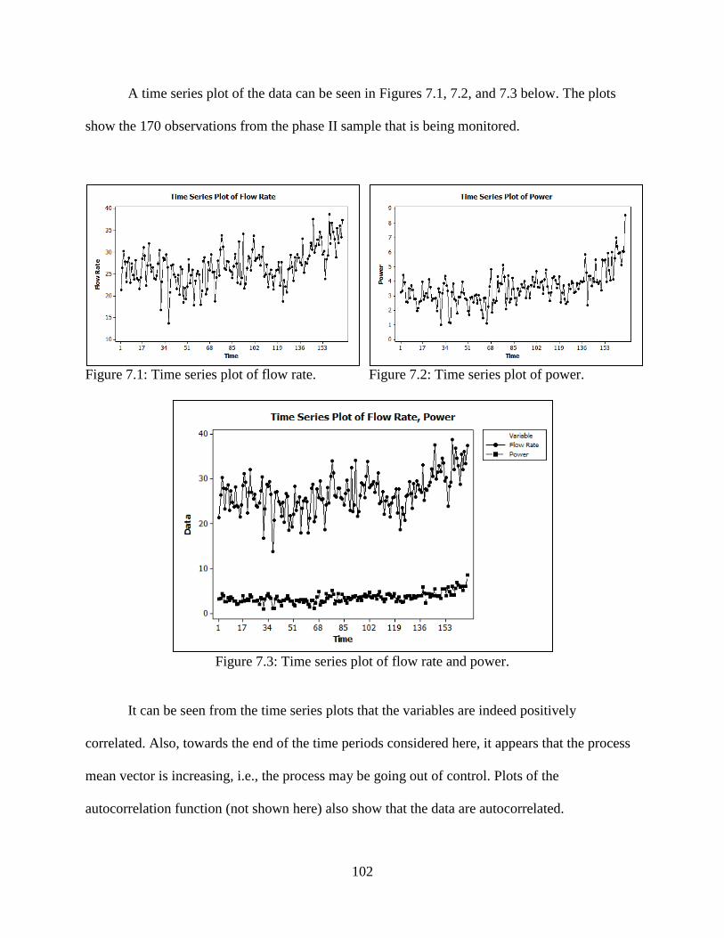
102

A time series plot of the data can be seen in Figures 7.1, 7.2, and 7.3 below. The plots

show the 170 observations from the phase II sample that is being monitored.

Figure 7.1: Time series plot of flow rate.

Figure 7.2: Time series plot of power.

Figure 7.3: Time series plot of flow rate and power.

It can be seen from the time series plots that the variables are indeed positively

correlated. Also, towards the end of the time periods considered here, it appears that the process

mean vector is increasing, i.e., the process may be going out of control. Plots of the

autocorrelation function (not shown here) also show that the data are autocorrelated.

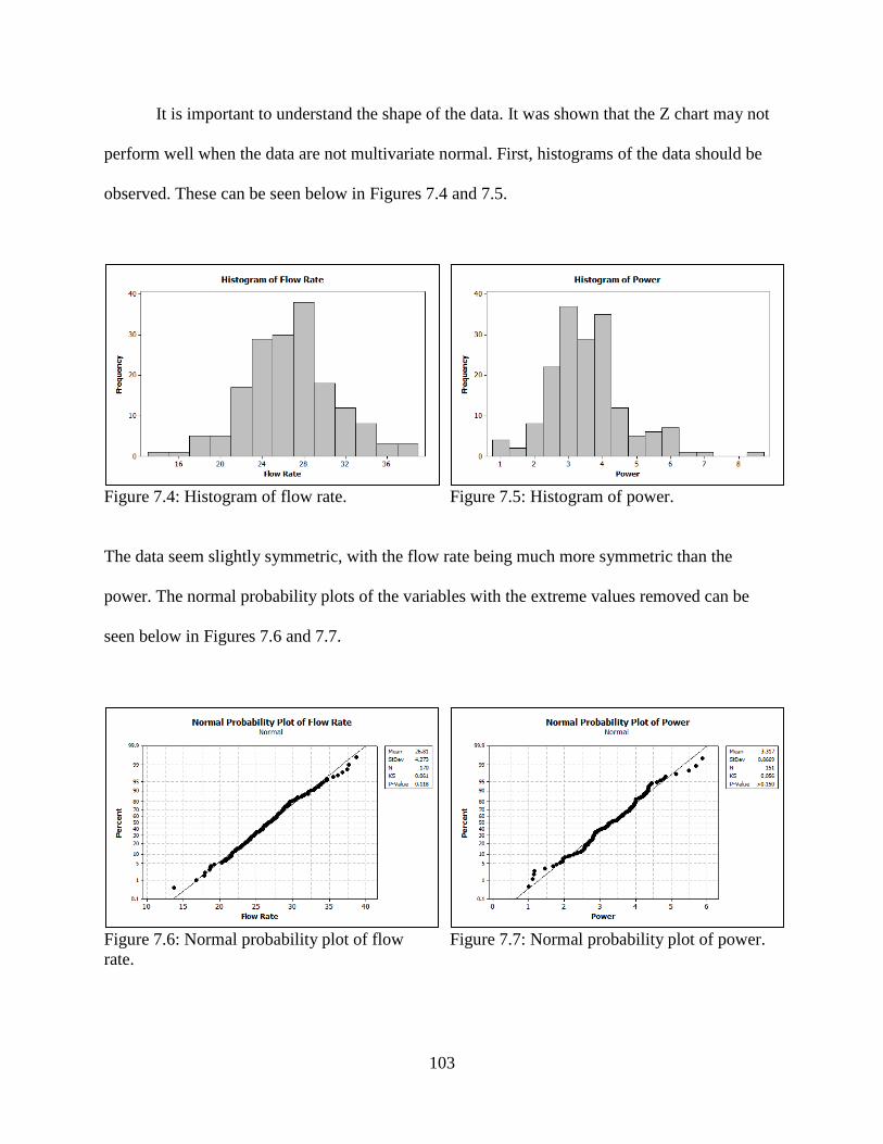
103

It is important to understand the shape of the data. It was shown that the Z chart may not

perform well when the data are not multivariate normal. First, histograms of the data should be

observed. These can be seen below in Figures 7.4 and 7.5.

Figure 7.4: Histogram of flow rate.

Figure 7.5: Histogram of power.

The data seem slightly symmetric, with the flow rate being much more symmetric than the

power. The normal probability plots of the variables with the extreme values removed can be

seen below in Figures 7.6 and 7.7.

Figure 7.6: Normal probability plot of flow

rate.

Figure 7.7: Normal probability plot of power.

104

It seems that the data are not far from normal, so we will be assuming normality here.

Thus, the data are acceptable for the application of the Z chart.

7.2.2 Results

For the Z chart to be applied, the mean, variance, and covariance of the data need to be

known. With a large amount of holdout data, these parameters can be estimated with a high sense

of accuracy. In this case, 324 phase I observation vectors were used to estimate the parameters. It

was shown in Chapter 4 that a sample of at least 200 observation vectors is sufficient for the

chart to perform desirably, so the sample size in this process is acceptable. Note that the

covariance will be used in the calculation of the upper control limit using the regression model

presented in Chapter 4. The following values of the parameters were found:

Using the estimate of the covariance, the estimated upper control limit is

The Z chart applied to the data can be seen below in Figure 7.8.

105

Figure 7.8: Z chart applied to the hydroelectric data.

The chart also begins to show that the process goes out of control, trending upwards

starting around time point 127 and signaling at time point 138 and again at 146 before multiple

sequential points signal.

Recall that a benefit of the Z chart is the determination of the variable or variables that

provide the multivariate chart to signal. To determine which values led to the signal, we only

need to see the individual statistic values at the time points where a signal was detected. We may

also observe the chart of individual statistics at the points where a multivariate signal was

detected. Assuming the first two signals were simply false alarms, the plots of the individual Z

statistics are created for the 138th

time point onward. These plots can be seen below in Figures

7.9 and 7.10.

0

1

2

3

4

5

6

7

1

10

19

28

37

46

55

64

73

82

91

10

0

10

9

11

8

12

7

13

6

14

5

15

4

16

3

Z

Time

Z Chart

Z

UCL

106

Figure 7.9: Plot of Z for flow rate.

Figure 7.10: Plot of Z for power.

From the plots of the statistics of the individual variables, it can be seen that the values

for power contributed to most of the multivariate signals. This may indicate that a problem has

occurred with the generator. Note also that the chart of the flow rate signals three times, so some

of the signals seen in the power variable may be due to fluctuations in the flow rate as well.

7.3 Application of the New Nonparametric Charts

7.3.1 Description of Data

For the application of the proposed nonparametric charts, data was obtained from a

manufacturing process including the creation of plastic components for automotive interiors and

other applications. The actual part of the process that is being monitored involves a spray gun

that sprays a molding compound onto a mold. The compound sets, yielding the plastic

component. Both the pressure and temperature of the compound is monitored. It is known that

temperature and pressure are related. Since there is some relationship between the two variables,

a multivariate control chart would be appropriate to monitor the two variables of the process. The

process also includes an automatic adjustment feature that will adjust the equipment once a

signal has occurred.

0

1

2

3

4

13

8

14

1

14

4

14

7

15

0

15

3

15

6

15

9

16

2

16

5

16

8

Time

Z for Flow Rate

Z(FR)

UCL01234567

13

8

14

1

14

4

14

7

15

0

15

3

15

6

15

9

16

2

16

5

16

8

Time

Z for Power

Z(Pwr)

UCL

107

The mechanics of the process remained unchanged for 5 years, yielding a very large

amount of data from which to estimate the parameters. The parameters were estimated with

5,353 observation vectors, so it is expected that the parameters will be estimated with great

accuracy. Only a small portion of phase II data was considered here. A time series plot of the two

variables can be seen below in Figures 7.11, 7.12, and 7.13.

Figure 7.11: Time series plot of the means of

pressure.

Figure 7.12: Time series plot of the means of

temperature.

Figure 7.13: Time series plot of the means of pressure and temperature.

108

It can be seen that there is a slight negative relationship between the two variables. The

linear correlation coefficient was found to be -0.138, which will be used in determining the

control limits of the maximum sign and signed-rank charts. The process means were found to be

47.66 and 72.70 for the pressure and temperature, respectively. The process medians were found

to be 47.58 and 72.68.

The shape of the data should also be considered. Histograms of the variables can be seen

in Figures 7.14 and 7.15 below.

Figure 7.14: Histogram of pressure.

Figure 7.15: Histogram of temperature.

It seems that the data are slightly skewed. If a portion of the data was removed, the pressure

variable may be slightly symmetric. This implies that the charts based on the signed-rank statistic

may be able to detect a shift quicker than those that are based on the sign statistic, as noted in

Chapter 6. The normality of the data will also be observed. The normal probability plot of the

two variables (after removing a large portion of outlying observations which may be out of

control) can be seen below in Figures 7.16 and 7.17.

109

Figure 7.16: Normal probability plot of

pressure (individual values).

Figure 7.17: Normal probability plot of

temperature (individual values).

It seems that the normality assumption of the data is violated. It may then be erroneous to use

charts that require the normality assumption to be valid, such as Hotelling‟s T2 chart. A desirable

alternative may be one of the proposed nonparametric charts.

In the following section, Hotelling‟s T2 chart and the four proposed nonparametric charts

will be applied to this stage of the process.

7.3.2 Results

When Hotelling‟s T2 chart is applied to the section of phase II data, signals can be seen at

multiple time points. The results can be seen below in Figure 7.18.

110

Figure 7.18: Hotelling‟s T

2 chart of pressure and temperature.

The T2 chart shows some signals early in this section of the process, but the process

seems to be out of control starting near time point 22. Recall that an automatic adjustment is

made when the process goes out of control, which can be seen near time point 31.

Applying the new charts show similar results. Note that only the in-control median needs

to be known for the application of the multivariate sign and signed-rank charts and the maximum

sign and signed-rank charts require the in-control median and the correlation matrix. Each of

these has been estimated from a very large amount of data, so the chart will be applied using

these estimated parameters.

For the multivariate sign and signed-rank charts, the lower control limit is 0 and the upper

control limit is . The upper control limit for the maximum sign and signed-rank

charts were found by simulation. These are found to be 3.0267 the maximum sign chart and

3.0275 for the maximum signed-rank chart. Note that these are very similar since the correlation

between the variables is relatively low, i.e., of the correlation is not far from the correlation

itself.

The results of the application of the new charts can be seen below in Figures 7.19-7.22.

37332925211713951

400

300

200

100

0

Time

Tsq

ua

red

UCL=13.0

Tsquared Chart of Pressure and Temperature

111

Figure 7.19: Multivariate sign chart applied to the phase II process data.

Figure 7.20: Multivariate signed-rank chart applied to the phase II process data.

112

Figure 7.21: Maximum sign chart applied to the phase II process data.

Figure 7.22: Maximum signed-rank chart applied to the phase II process data.

113

Each chart detects each of the signals just as Hotelling‟s T2 chart does. Note that there are

some points on which the charts do not agree. For example, at point 12, each of the new charts

and the parametric chart signal, but the maximum sign chart does not. The vector of observation

means at that point is (46.684, 72.785). The pressure is slightly below the mean and the

temperature is slightly above, which often yields a multivariate signal. It is unclear of why the

maximum sign chart does not signal at that point. It may be due to the symmetric nature of the

process. Recall that if the process data is symmetric, the charts based on Wilcoxon signed-rank

statistics will be slightly more powerful, or may detect a shift better than, the charts based on the

sign statistic. Note also that there are points where the sign charts signal and the signed-rank

charts do not. For example, the sign charts signal at time point 18, as does the parametric chart.

Note that for the maximum sign and signed-rank charts, it is possible to immediately

determine which variable or variables contributed to the signal. To show the benefit of this

diagnostic ability, plots of the statistics of the individual variables are created for the maximum

signed-rank chart. These can be seen below in Figures 7.23 and 7.24.

Figure 7.23: Plot of univariate signed-rank

statistics for pressure.

Figure 7.24: Plot of univariate signed-rank

statistics for temperature.

114

It can be seen from the plots of the statistics of the individual variables that both seem to

contribute greatly to the signals on the multivariate chart. The pressure contributes to more

signals, but since there are many points that signal on the plot of temperature as well, we may

conclude that both variables are out of control.

7.4 Conclusion

For the application of the Z chart, it was very beneficial to have data that appears to be

close to normal and that a large phase I sample was provided. Thus, the results of the chart are

expected to be accurate. It was found that the process remained in control for most of the section

of phase II data that was considered with only two false alarms before the process was

determined to be out of control. Using the Z chart, it was also possible to determine which

variable contributed to the signal, so individual plots of the statistics were created, showing that

the changes in power contributed more to the signals.

For the application of the nonparametric charts, the benefit of a large phase I sample was

also clear. The data were shown to be non-normal, which is acceptable for the use of the

nonparametric charts. All charts showed multiple signals, as did Hotelling‟s T2 chart. Using the

maximum sign and signed-rank charts, it was shown that both variables were out of control.

115

CHAPTER 8

CONCLUSION

8.1 Summary

Many problems arise when working with multivariate autocorrelated data or when the

process does not follow a multivariate normal distribution (or the distribution of the process is

unknown). Both of these cases were examined in the dissertation. For multivariate autocorrelated

data, properties of the Z chart, presented by Kalgonda and Kulkarni (2004), including a

performance comparison and its robustness to parameter estimation and multivariate normality,

were studied. For non-normal cases, four new multivariate nonparametric control charts were

presented and studied.

In Chapter 3, the Z chart was compared to Hotelling‟s χ2 chart and the MEWMA chart

assuming that the parameters are known and the data is distributed multivariate normal. Setting

the in-control ARL to be equal, the out-of-control performance of the charts was studied. The Z

chart was outperformed by the other two in most cases. However, it is important to note that the

Z chart has the added benefit of determining which of the variables are out of control.

In Chapter 4, the effects of parameter estimation on the performance of the Z chart were

explored. When parameters are estimated, it was seen that the performance of the chart is

degraded when the process is non-normal in the sense that the desired in-control ARL is not

obtained. It was also seen that a sample of approximately 200 vectors seems to alleviate the

estimation issue. Tables are presented to provide a means for determining possible choices

116

of estimating sample sizes and for determining the amount of error inherent in using the Z chart

for certain sample sizes.

In Chapter 5, the performance of the Z chart when the data are not multivariate normal

was studied. As expected, it was seen that the performance of the chart is degraded when the

process data do not come from a normal distribution. When the data are far from multivariate

normal, the in-control ARL is far from the desired. The chart deteriorates similarly for both non-

normal symmetric and asymmetric distributions. However, when the data are near normal, the

use of the chart may be justified. It is important to note that it may be very difficult to determine

whether or not the data are near normal, so distribution-free (or nearly distribution-free) charts

should be considered.

In Chapter 6, four new nonparametric charts were proposed. The new charts are based on

the multivariate sign and signed-rank statistics and the maximum of univariate sign and signed-

rank statistics. They are relatively easy to use and are distribution-free for large samples. The

performance of the new charts was also explored. The new charts have a higher-than-nominal in-

control average run length but still can detect shifts relatively well. As the sample size increases,

the in-control ARL approaches the nominal value.

In Chapter 7, applications of the Z chart and the proposed nonparametric charts were

examined. The Z chart was applied to data from a hydroelectric process including the monitoring

of the flow rate of water flowing into the facility and the output power of the generator. The

chart was able to detect when the process went out of control and determine which variable

caused the signal. The nonparametric charts were applied to data from a manufacturing process

involving a spray gun applying a compound onto a mold for the construction of plastic

components. The pressure and temperature of the compound were monitored. The data were

117

non-normal, which is not a problem for the nonparametric charts. The charts showed that the

process was out of control. The maximum sign and signed-rank charts also showed that both

variables were out of control.

8.2 Future Research

In the Z chart and the nonparametric charts presented in this paper, only the bivariate

cases were considered. The performance and robustness properties of these charts may be

slightly different for larger dimensions, so this should be studied. Finding the control limit for

the Z chart is also a time-consuming process. A theoretical method relating the covariance matrix

of the data to the control limit should be developed to facilitate the use of the charts.

More work should be done with the nonparametric charts proposed in this dissertation.

First, for example, the in-control mean (or median) was assumed known. It may be useful to

study situations and adaptations when this is not the case and the mean (or median) is estimated.

Second, the simulations were performed using bivariate data, so the performance of the charts

with more than two variables needs to be studied. Third, for the maximum sign and signed-rank

charts, the correlation matrix was assumed known while finding the upper control limit. The

effects of the estimation of the correlation matrix should also be studied. Fourth, it will be useful

to study the performance of the charts when the distribution of the process is not symmetric.

Fifth, other uses of the sign and signed-rank statistics, such as multivariate CUSUM-type or

multivariate EWMA-type charts should be considered. Finally, it may be important to consider

nonparametric statistics other than the sign and signed-rank statistics in the construction of

control charts.

118

REFERENCES

Adams, B. M. and Tseng, I. (1998). Robustness of forecast-based monitoring schemes, Journal

of Quality Technology, Vol. 30(4), pp. 328-339.

Akkaya, A. and Tiku, M. L. (2001). Estimating parameters in autoregressive models in non-

normal situations: asymmetric innovations, Communications in Statistics – Theory and Methods,

Vol. 30(3), pp. 517-536.

Albers, W. and Kallenberg, W. C. M (2006). Alternative Shewhart-type charts for grouped

observations, Metron LXIV, pp. 357-375.

Alwan, A. J. and Alwan, L. C. (1994). Monitoring autocorrelated processes using multivariate

quality control charts, Proceedings of the Decision Sciences Institute Annual Meeting, Vol. 3, pp.

2106-2108.

Alwan, B.M. and Roberts, H.V. (1988). Time-series modeling for detecting level shifts of

autocorrelated processes, Journal of Business and Economic Statistics, Vol. 6 (1), pp. 87-96.

Anderson, T. W. (1984). An Introduction to Multivariate Statistical Analysis, 2nd

Ed., John Wiley

and Sons, New Jersey.

Aparisi, F., Champ, C. W., and Garcia-Diaz, J. C. (2004). A performance analysis of Hotelling‟s

T2 control chart with supplementary runs rules, Quality Engineering, 16(3), pp. 359-368.

Apley, D. W. and Tsung, F. (2002). The autoregressive T2 chart for monitoring univariate

autocorrelated processes, Journal of Quality Technology, Vol. 34(1), pp. 80-96.

Bakir, S. T. (2004). A distribution-free Shewhart quality control chart based on signed-ranks,

Quality Engineering, 16(4), pp. 613-623.

Bakir, S. T. and Reynolds, M. R. (1979). A nonparametric procedure for process control based

on within-groups ranking, Technometrics, Vol. 21(2), pp. 175-183.

Balakrishnan, N., Triantafyllou, I. S., and Koutras, M. V. (2009). Nonparametric control charts

based on runs and Wilcoxon-type rank-sum statistics, Journal of Statistical Planning and

Inference, Vol. 139, pp. 3177-3192.

119

Bersimis, S., Psarakis, S., and Panaretos, J. (2007). Multivariate statistical process control charts,

Quality and Reliability Engineering International, Vol. 23, pp. 517-543.

Borror, C. M., Montgomery, D. C., and Runger, G. C. (1999). Robustness of the EWMA control

chart to nonnormality, Journal of Quality Technology, Vol. 31(3), pp. 309-316.

Box, G. E., Jenkins, G. M., and Reinsel, G. C. (2008). Time Series Analysis: Forecasting and

Control, 4th

ed., John Wiley and Sons, New Jersey.

Chakraborti, S. and Eryilmaz, S. (2007). A nonparametric Shewhart-type signed-rank control

chart based on runs, Communications in Statistics – Simulation and Computation, 36(2), pp. 335-

356.

Chakraborti, S. and Graham, M. A. (2007). Nonparametric control charts, Encyclopedia of

Quality and Reliability, John Wiley, New York.

Chakraborti, S. and van de Wiel, M. A. (2008) A nonparametric control chart based on the

Mann-Whitney statistic, Beyond parametrics in interdisciplinary research: Festschrift in honor

of Professor Pranab K. Sen, pp. 156-172, Balakrishnan, N. (ed.), Peña, Edsel A. (ed.) and

Silvapulle, Mervyn J. (ed.), Institute of Mathematical Statistics (Hayward).

Chakraborti, S., van der Laan, P., and Bakir, S. T. (2001). Nonparametric control charts: an

overview and some results, Journal of Quality Technology, Vol. 33(3), pp. 304-315.

Champ, C. W. and Aparisi, F. (2007). Double sampling Hotelling‟s T2 charts, Quality and

Reliability Engineering International, Vol. 24, pp. 153-166.

Champ, C. W., and Jones-Farmer, L. A. (2007). Properties of multivariate control charts with

estimated parameters, Sequential Analysis, Vol. 26, pp. 153-169.

Champ, C. W., Jones-Farmer, L. A., and Rigdon, S. E. (2005). Properties of the T2 control chart

when parameters are estimated, Technometrics, Vol. 47(4), pp. 437-445.

Chatterjee, S. and Qiu, P. (2009). Distribution-free cumulative sum control charts using

bootstrap-based control limits, The Annals of Applied Statistics, Vol. 3, pp. 349-369.

Cherubini, U., Luciano, E., and Vecchiato, W. (2004). Copula Methods in Finance, John Wiley

and Sons, New Jersey.

Chou, Y., Mason, R. L. and Young, J. C. (2001). The control chart for individual observations

from a multivariate non-normal distribution, Communications in Statistics - Theory and

Methods, Vol. 30(8), pp. 1937-1949.

Crosier, R.B. (1988). Multivariate generalizations of cumulative sum quality control schemes,

Technometrics, Vol. 30(3), pp. 291-303.

120

Das, N. (2009). A new multivariate non-parametric control chart based on the sign test, Quality

Technology & Quantitative Management, Vol. 6(2), pp. 155-169.

Dyer, J. N., Conerly, M. D., and Adams, B. M. (2003). A simulation study and evaluation of

multivariate forecast based control charts applied to ARMA processes, Journal of Statistical

Computation and Simulation, Vol. 73(10), pp. 709-724.

Gibbons, J. D. and Chakraborti, S. (2003). Nonparametric Statistical Inference, 4th

ed., Marcel

Dekker, New York.

Graham, M. A., Human, S. W. and Chakraborti, S. (2009). A nonparametric Phase I control

chart, Journal of Applied Statistics, Accepted.

Hamurkaroglu, C., Mert, M., and Saykan, Y. (2004). Nonparametric control charts based on

Mahalanobis depth, Hacettepe Journal of Mathematics and Statistics, Vol. 33, pp. 57-67.

Hancock, G. and Klockars, A. (1997). Finite intersection tests: a paradigm for optimizing

simultaneous and sequential inference, Journal of Education and Behavioral Statistics, Vol.

22(3), pp. 291-307.

Harris, T. J. and Ross, W. H. (1991). Statistical process control procedures for correlated

observations, The Canadian Journal of Chemical Engineering, Vol. 69, pp. 48-57.

Hayter, A. J. and Tsui, K. (1994). Identification and quantification in multivariate quality control

problems, Journal of Quality Technology, Vol. 26(3), pp. 197–208.

Healy, J. D. (1987). A note on multivariate CUSUM procedures, Technometrics, Vol. 29, pp.

409-412.

Hettmansperger, T. P. (2006). Multivariate location tets, Encyclopedia of Statistical Sciences,

John Wiley and Sons, New Jersey.

Hotelling, H. (1947). Multivariate quality control illustrated by the air testing of sample

bombsights. Techniques of Statistical Analysis, Eisenhart, C., Hastay, M.W., and Wallis, W.A.

(eds.), McGraw-Hill, New York, pp. 111-184.

Hwarng, H. B. (2008). Toward identifying the source of mean shifts in multivariate SPC: a

neural network approach. International Journal of Production Research, 46(20), pp. 5531-5559.

Hwarng, H. B. and Wang, Y. (2008). Shift detection and source identification in multivariate

autocorrelated processes. International Journal of Production Research, DOI:

10.1080/00207540802431326.

Jarrett, J. E. and Pan, X. (2007). The quality control chart for monitoring multivariate

autocorrelated processes, Computational Statistics and Data Analysis, Vol. 51, pp. 3862-3870.

121

Jensen et al. (2006). Effects of parameter estimation on control chart properties: a literature

review, Journal of Quality Technology, Vol. 38(4), pp. 349-364.

Jensen, W. A., Birch, J. B., and Woodall, W. H. (2007). High breakdown estimation methods for

phase I multivariate control charts, Quality and Reliability Engineering International, Vol. 23,

pp. 615-629.

Johnson, N. L. and Kotz, S. (1976). Distributions in Statistics: Continuous Multivariate

Distributions, John Wiley, New York.

Johnson, R. A. and Wichern, D. W. (2007). Applied Multivariate Statistical Analysis, 6th

ed,

Pearson Education, New Jersey.

Joner Jr., M. D., Woodall, W. H., Reynolds Jr., M. R. and Fricker Jr., R. D. (2008). A one-sided

MEWMA chart for health surveillance, Quality and Reliability Engineering International, Vol.

24, pp. 503-518.

Jones-Farmer, L. A., Jordan, V., and Champ, C. W. (2009). Distribution-free phase I control

charts for subgroup location, Journal of Quality Technology, Vol. 41(3), pp. 304-316.

Kalgonda, A. A. and Kulkarni, S. R. (2004). Multivariate quality control chart for autocorrelated

processes, Journal of Applied Statistics, Vol. 31(3), pp. 317-327.

Kang, K. and Schmeiser, B. (1987). Properties of batch means from stationary ARMA time

series, Operations Research Letters, Vol. 6, pp. 19-24.

Kapatou, A. and Reynolds Jr., M. R. (1994). Multivariate nonparametric control charts using

small samples. ASA Proceedings of the Section on Quality and Productivity, pp. 241-246.

American Statistical Association (Alexandria, VA).

Kapatou, A. and Reynolds Jr., M. R. (1998). Multivariate nonparametric control charts for the

case of known sigma, ASA Proceedings of the Section on Quality and Productivity, pp. 77-82,

American Statistical Association (Alexandria, VA).

Kear, F. W. (1998). Statistical Process Control in Manufacturing Practice, Marcel Dekker, New

York.

Kotz, S and Nadarajah, S. (2004). Multivariate t Distributions and Their Applications,

Cambridge University Press, Cambridge.

Kourti, T. and MacGregor, J. F. (1996). Multivariate SPC methods for process and product

monitoring, Journal of Quality Technology, Vol. 28, pp. 409-428.

Kramer, H. and Schmid, W. (2000). The influence of parameter estimation on the ARL of

Shewhart type charts for time series, Statistical Papers, Vol. 41, pp. 173-196.

122

Krishnamoorthy, A. S. and Parthasarathy, M. (1951). A multivariate gamma-type distribution,

The Annals of Mathematical Statistics, Vol. 22(4), pp. 549-557.

Lee, M. H. and Khoo, M. (2006). Optimal statistical design of a multivariate EWMA chart based

on ARL and MRL, Communications in Statistics: Simulation and Computation, Vol. 35, 831-

847.

Lin, W. S. W. and Adams, B. M. (1996). Combined control charts for forecast-based monitoring

schemes, Journal of Quality Technology, Vol. 28(3), pp. 289-301.

Liu, R. Y. (1990). On a notion of data depth based on random simplices, The Annals of Statistics,

Vol. 18, pp. 405-414.

Liu, R. Y. (1995). Control charts for multivariate processes, Journal of the American Statistical

Association, Vol. 90(432), pp. 1380-1387.

Liu, R. Y., Singh, K., and Teng, J. H. (2004). DDMA-charts: nonparametric multivariate moving

average control charts based on data depth, Allgemeines Statistisches Archiv, Vol. 88, pp. 235-

258.

Lowry, et al. (1992). A multivariate exponentially weighted moving average control chart,

Technometrics, Vol. 34(1), pp. 46-53.

Lowry, C. and Montgomery, D. (1995). A review of multivariate control charts, IIE

Transactions, Vol. 27, pp. 800-810.

Lu, C. W. and Reynolds, M. R. Jr. (1991). Control charts for monitoring the mean and variance

of autocorrelated processes, Journal of Quality Technology, Vol. 31(3), pp. 259–273.

Lütkepohl, H. (1991). Introduction to Multiple Time Series Analysis, Springer-Verlag, Berlin.

Mason, R. L. and Young, J. C. (2002). Multivariate Statistical Process Control with Industrial

Applications, American Statistical Association – Society for Industrial and Applied Mathematics,

Philadelphia.

Mason, R. L. et al. (1997). Assessment of multivariate process control techniques, Journal of

Quality Technology, Vol. 29(2), pp. 140-143.

Mason, R. L., Chou, Y., and Young, J. C. (2001). Applying Hotelling‟s T2 statistic to batch

processes, Journal of Quality Technology, Vol. 33(4), pp. 466-479.

Mastrangelo, M. C., Runger, G. C. and Montgomery, D. C. (1996). Statistical process

monitoring with principal components. Quality and Reliability Engineering International,

Vol. 12(3), pp. 203-210.

123

Montgomery, D. C. (2005). Statistical Quality Control, 5th

ed., John Wiley and Sons, New

Jersey.

Oja, H. and Randles, R. H. (2004). Multivariate nonparametric tests, Statistical Science, Vol.

19(4), pp. 598-605.

Pan, X. and Jarret, J. (2007). Using vector autoregressive residuals to monitor multivariate

processes in the presence of serial correlation. International Journal of Production Economics,

Vol. 106(1), pp. 204-216.

Pignatiello, J. J., Jr. and Runger, G. C. (1990). Comparisons of multivariate CUSUM

charts, Journal of Quality Technology, Vol. 22, pp. 173-186.

Prabhu, S. S. and Runger, G. C. (1997). Designing a multivariate EWMA control chart, Journal

of Quality Technology, Vol. 29(1), pp. 8-15.

Psarakis, S. and Papaleonida, G. E. A. (2007). SPC Procedures for Monitoring

Autocorrelated Processes, Quality Technology and Quantitative Management, Vol. 4(4), pp.

501-540.

Puri, M. L. and Sen, P. K. (1976). Nonparametric Methods in Multivariate Analysis, John

Wiley, New York.

Qiu, P. and Hawkins, D. (2001). A rank-based multivariate CUSUM procedure, Technometrics,

Vol. 43, No. 2, pp. 120-132.

Reinsel, G. C. (1993). Elements of Multivariate Time Series Analysis, Springer, New York.

Rousseeuw, P. J. (1984). Least median of squares regression, Journal of the American Statistical

Association, Vol. 79, pp. 871-880.

Rousseeuw, P. J. and van Driessen, K. (1999). A fast algorithm for the minimum covariance

determinant estimator, Technometrics, Vol. 41, pp. 212-223.

Rousseeuw, P. J. and van Zomeren, B. C. (1990). Unmasking multivariate outliers and leverage

points, Journal of the American Statistical Association, Vol. 85, pp. 633-651.

Runger, G. C. and Willemain, T. R. (1995). Model-based and model-free control of

autocorrelated processes, Journal of Quality Technology, Vol. 27(4), pp. 283-292.

Shäfer, J. and Strimmer, K. (2005). A shrinkage approach to large-scale covariance matrix

estimation and implications for functional genomics, Statistical Applications in Genetics

and Molecular Biology, Vol. 4(1), Article 32.

Schilling, E. G. and Nelson, P. R. (1976). The effect of non-normality on the control limits of

charts, Journal of Quality Technology, Vol. 8, pp. 183-188.

124

Stoumbos, Z. G. and Sullivan, J. H. (2002). Robustness to non-normality of the multivariate

EWMA control chart, Journal of Quality Technology, Vol. 34(3), pp. 260-276.

Sullivan, J. H. and Stoumbos, Z. G. (2001). Achieving robust performance with the MEWMA

control chart, ASA Proceedings of the Joint Statistical Meetings, American Statistical

Association (Alexandria, VA).

Timm, N. H. (1996). Multivariate quality control using finite intersection tests, Journal of

Quality Technology, Vol. 28, pp. 233-243.

Tracy, N. D., Young, J. C., and Mason, R. L. (1992). Multivariate control charts for individual

observations, Journal of Quality Technology, Vol. 24(2), pp. 88-95.

Tseng, S. and Adams, B. M. (1994). Monitoring autocorrelated processes with an exponentially

weighted moving average forecast, Journal of Statistical Computation and Simulation, Vol.

50(3-4), pp. 187-195.

Tsionas, E. (2004). Bayesian inference for multivariate gamma distribution, Statistics and

Computing, Vol. 14, pp. 223-233.

Vargas, J. A. (2003). Robust estimation in multivariate control charts for individual observations,

Journal of Quality Technology, Vol. 35(4), pp. 367-376.

Vasilopoulos, A. V. and Stamboulis, A. P. (1978). Modification of control chart limits in the

presence of data correlation, Journal of Quality Technology, Vol. 10(1), pp. 20-30.

Wardell, D. G., Moskowitz, H. and Plante, R. D. (1994). Run-length distributions of

special-cause control charts for correlated process. Technometrics, Vol. 36(1), 3-27.

Wetherill, G. B. and Brown, D. W. (1991). Statistical Process Control: Theory and Practice,

Chapman and Hall, London.

Willemain, T. R. and Runger, G. C. (1996). Designing control charts based on an empirical

reference distribution, Journal of Quality Technology, Vol. 28(1), pp. 31-38.

Woodall, W. H. and Montgomery, D. C. (1999). Research issues and ideas in statistical process

control, Journal of Quality Technology, Vol. 31(4), pp. 376-386.

Woodall, W. H. and Ncube, M. M. (1985). Multivariate CUSUM quality control

procedures, Technometrics, Vol. 27, pp. 285-292.

Yourstone, S. A. and Zimmer, W. J. (1992). Non-normality and the design of control charts for

averages, Decision Sciences, Vol. 23(5), pp. 1099-1113.

125

APPENDIX A

THE MULTIVARIATE T DISTRIBUTION

The multivariate t distribution, also called the multivariate Student distribution, is simply

the multivariate analog of the Student‟s t distribution. It is similar to the multivariate normal

distribution in that it is symmetric, but with a larger kurtosis. It has recently become popular in

finance (Cherubini, Luciano, and Vecchiato, 2004). Similar to the definition in Kotz and

Nadarajah (2004) and Johnson and Kotz (1976), let y and µ be independent with y distributed as

multivariate normal with zero mean vector and covariance matrix and u distributed as chi-

squared with ν degrees of freedom. Also, let . The probability density function

of x is then

for , x is the vector of observations, µ is the mean vector, ν is the degrees of

freedom, and , where p is the number of parameters. x is then said to follow a

multivariate t distribution with parameters µ, , and ν. The mean of the multivariate

distribution is µ and the covariance matrix is defined by

126

Table A.1: Skewness and kurtosis for univariate t distributions.

Distribution Skewness Kurtosis

Normal 0 3

t1(3) Indeterminate Indeterminate

t1(4) 0 Indeterminate

t1(5) 0 9

t1(6) 0 6

t1(10) 0 4

t1(20) 0 3.375

t1(40) 0 3.167

t1(100) 0 3.063

t1(1000) 0 3.006

t1(10000) 0 3.001

The table above, from Stoumbos and Sullivan (2002), shows that as the degrees of

freedom increases, the t distribution tends to the normal distribution. This translates to the

multivariate case with the multivariate t distribution tending to the multivariate normal

distribution.

127

APPENDIX B

THE MULTIVARIATE GAMMA DISTRIBUTION

The multivariate gamma distribution is simply the multivariate analog of the gamma

distribution. For the purpose of data generation, the Wishart distribution, named for John Wishart

(1928), will be used. Stoumbos and Sullivan (2002) used one-half the diagonal elements of a

matrix following the Wishart distribution when studying the robustness of the MEWMA chart to

non-normality, so the same generation technique will be used here The distribution has been

included in many multivariate texts, including Johnson and Wichern (2007) and Anderson

(1984), as well as many papers, including Krishnamoorthy and Parthasarathy (1951) and Tsionas

(2004). Let , with Z being a p x 1 vector following a multivariate normal distribution

with zero mean vector and covariance matrix . The probability density function of W is

given by

where W is the p x p matrix of observations, is the covariance matrix of the multivariate

normal distribution, ν is the scalar degrees of freedom with , and is the

multivariate gamma function given by

128

W is then said to follow a Wishart distribution with parameters and ν. Note here that

is the covariance matrix of the multivariate normal distribution; not the covariance matrix of the

Wishart distribution.

For the generation of a random vector from the multivariate gamma distribution, the

diagonal elements of the random matrix generated from the Wishart distribution will be

considered. Using the definition of the multivariate gamma distribution in Stoumbos and

Sullivan (2002), we will take one-half of these diagonal entries. This leads to the mean vector of

these elements being

the variance of the ith

variable is

, and the covariance between the i

th and j

th variable is

,

with being the ijth

component of the parameter of the Wishart distribution. Note that in

Stoumbos and Sullivan (2002), the mean is given by and the variance is given by , but

this is the mean and variance of the diagonal entries, not one-half the diagonal entries.

For the univariate analog of these distributions, as seen in Stoumbos and Sullivan (2002),

the skewness and kurtosis are summarized in Table B.1.

129

Table B.1: Skewness and kurtosis for univariate Gamma distributions.

Distribution Skewness Kurtosis

Normal 0 3

Gamma1(1,1) 2 9

Gamma1(4,1) 1 4.5

Gamma1(16,1) 0.5 3.375

Gamma1(64,1) 0.25 3.094

Gamma1(256,1) 0.125 3.023

Gamma1(1024,1) 0.063 3.006

Gamma1(4096,1) 0.031 3.001

Gamma1(16384,1) 0.016 3.000

From Table B.1, it can be seen that for the univariate Gamma distribution, as the shape

parameter increases, the skewness approaches zero and the kurtosis approaches 3. Thus, for

lower values of the shape parameter, the distribution is very skewed. As the parameter increases,

the distribution becomes more symmetric and more towards the normal distribution. This

translates to the multivariate case as well. As the shape parameter of the multivariate Gamma

distribution increases, the distribution tends to the multivariate normal distribution.

130

APPENDIX C

R PROGRAMS USED FOR SIMULATION

C.1 Programs from Chapter 3

vargen<-function (n,phi,mu,sig) {

#Generates random data from a VAR(1) model.

#Requires the MASS package to be loaded.

#n is the number of vectors to be generated.

#phi is the matrix of autocorrelation parameters.

#mu is the mean vector.

#sig is the error covariance matrix.

#Fix the mean vector to work in the following calculations.

mu<-t(t(mu))

#Initialize the matrix of VAR(1) data.

y<-matrix(0,length(mu),n)

#Generate the matrix of errors.

e<-t(mvrnorm(n,matrix(0,1,length(mu)),sig))

#Calculate the vector of data at the first time point.

y[,1]<-mu+e[,1]

#Calculate the remaining data vectors.

for(i in 2:n) {

y[,i]<-mu+phi%*%(y[,(i-1)]-mu)+e[,i]

}

#Return the matrix of generated data. A row represents a time point.

return(y)

}

czcalc<-function (nsim,mu,phi,sig,gam,eps,ll,ul) {

#Calculates the upper control limit of the Z chart for data coming

# from a given VAR(1) model.

#Performs a binary search to obtain an in-control ARL of 200.

#Calls the "zcalc" rogram.


#nsim is the number of simulations to calculate the ARL.

#mu is the in-control mean vector.

131



#gam is the cross-covariance matrix.

#eps is the difference in two ARL values upon convergence.

#ll is the lower limit of the UCL from which to start.

#ul is the upper limit of the UCL from which to start.

#Check if lower limit is too high (receives an ARL higher than 200.

rll<-mean(zcalc(nsim,mu,mu,phi,sig,gam,ll))

if(rll>200) {

print("Lower limit too high!")

return()

}

#Check if the upper limit is too low (receives an ARL lower than 200).

rlu<-mean(zcalc(nsim,mu,mu,phi,sig,gam,ul))

if(rlu<200) {

print("Upper limit too low!")

return()

}

#Calculate pains of control limits (an upper and lower bound) until

# the absolute difference in the ARL obtained by these limits is

# smaller than epsilon.

while(abs(rlu-rll)>eps) {

#Check if the average of the two run lengths is greater than 200. If

# this is true, let the upper limit be the average of the two.

if((rlu+rll)/2>200)

ul<-(ul+ll)/2

#I the average of the two run lengths is greater than 200,let

# the upper limit be the average of the two.

else

ll<-(ul+ll)/2

#Assign new values to the ARL of the upper and lower limits. Due to

# the high variation that may be present in the run length

# distribution, the ARL may not be above (below) 200 for the upper

# (lower) limit. If this is the case the ARL will be recalculated.


while(rll>200)



while(rlu<200)


}

#Return the average of the upper and lower limits.

return((ul+ll)/2)

}

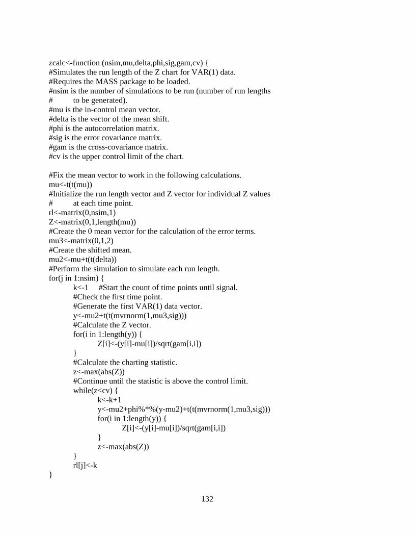
132

zcalc<-function (nsim,mu,delta,phi,sig,gam,cv) {

#Simulates the run length of the Z chart for VAR(1) data.


#nsim is the number of simulations to be run (number of run lengths

# to be generated).


#delta is the vector of the mean shift.

#phi is the autocorrelation matrix.



#cv is the upper control limit of the chart.


mu<-t(t(mu))

#Initialize the run length vector and Z vector for individual Z values

# at each time point.

rl<-matrix(0,nsim,1)

Z<-matrix(0,1,length(mu))

#Create the 0 mean vector for the calculation of the error terms.

mu3<-matrix(0,1,2)

#Create the shifted mean.

mu2<-mu+t(t(delta))

#Perform the simulation to simulate each run length.

for(j in 1:nsim) {

k<-1 #Start the count of time points until signal.

#Check the first time point.

#Generate the first VAR(1) data vector.

y<-mu2+t(t(mvrnorm(1,mu3,sig)))

#Calculate the Z vector.

for(i in 1:length(y)) {

Z[i]<-(y[i]-mu[i])/sqrt(gam[i,i])

}

#Calculate the charting statistic.

z<-max(abs(Z))

#Continue until the statistic is above the control limit.

while(z<cv) {

k<-k+1

y<-mu2+phi%*%(y-mu2)+t(t(mvrnorm(1,mu3,sig)))



}

z<-max(abs(Z))

}

rl[j]<-k

}

133

#Return the vector of simulated run lengths.

return(rl)

}

t2calc<-function (nsim,mu,delta,phi,sig,gam,cv) {

#Simulates the run length of the chi-squared chart for VAR(1) data.



# to be generated).








mu<-t(t(mu))






mu3<-matrix(0,2,1)


mu2<-mu+t(t(delta))


for(i in 1:nsim) {






t2<-t(y-mu)%*%solve(gam)%*%(y-mu)


while(t2<cv) {

k<-k+1

y<-mu2+phi%*%(y-mu2)+mvrnorm(1,mu3,sig)

t2<-t(y-mu)%*%solve(gam)%*%(y-mu)

}

rl[i]<-k

}


return(rl)

}

134

mewcalc<-function (nsim,mu,delta,phi,sig,gam,r,cv) {

#Simulates the run length of the MEWMA chart for VAR(1) data.



# to be generated).






#r is the parameter of the MEWMA chart.



mu<-t(t(mu))






mu3<-matrix(0,2,1)


mu2<-mu+t(t(delta))


for(i in 1:nsim) {





#Calculate the sigma matrix for the MEWMA statistic.

sigz<-(r/(2-r))*(1-(1-r)^2)*gam

#Calculate the initial z value.

z<-mu3


mew<-t(z)%*%solve(sigz)%*%z


while(mew<cv) {

k<-k+1

y<-mu2+phi%*%(y-mu2)+t(t(mvrnorm(1,mu3,sig)))

sigz<-(r/(2-r))*(1-(1-r)^(2*k))*gam

z<-r*y+(1-r)*z

mew<-t(z)%*%solve(sigz)%*%z

}

rl[i]<-k

}


135

return(rl)

}

zmastersim<-function (nsim,mu,phi,sig,gam,delta,cv) {

#Performs a run length simulation for a matrix of vectors of shifts for the

# Z chart.

#Calls the "zcalc" program.


#nsim is the number of simulations for each shift.





#delta is the matrix of vectors of shifts, where the vectors are

# arranged vertically, i.e., the first column is the first shift.


#Initialize the vector of run lengths. Each new run length vector will be

# cbind-ed to it.


#Simulate the run length vector for each column of the delta matrix.

for(i in 1:length(delta[1,])) {

rl<-cbind(rl,zcalc(nsim,mu,delta[,i],phi,sig,gam,cv))

}

#Remove the initial column of 0's.

rl<-rl[,-1]

#Return the matrix of run lengths with each column representing each shift.

return(rl)

}

t2mastersim<-function (nsim,mu,phi,sig,gam,delta,cv) {


# chi-squared chart.

#Calls the "t2calc" program.










136


# cbind-ed to it.




rl<-cbind(rl,t2calc(nsim,mu,delta[,i],phi,sig,gam,cv))

}


rl<-rl[,-1]


return(rl)

}

mewmastersim<-function (nsim,mu,phi,sig,gam,delta,r,cv) {


# Z chart.

#Calls the "zcalc" program.









#r is the parameter of the MEWMA chart.



# cbind-ed to it.




rl<-cbind(rl,mewcalc(nsim,mu,delta[,i],phi,sig,gam,r,cv))

}


rl<-rl[,-1]


return(rl)

}

137

C.2 Programs for Chapter 4

icstudy<-function (nsim,n,mu,phi,sig,gam,cv) {

#Finds known in-control case for Chapter 4 (Estimation), as seen in

# Table 4.2.

#Calls the "vargen" and "zcalc" programs which requires the MASS

# package to be loaded.

#nsim is the number of simulations to perform.

#n is the size of the sample from which the parameters are to be estimated.

#mu is the in-control mean.



#gam is the cross-covariance matrix of the process.


#Initialize the run length vector.

rlz<-matrix(0,nsim,1)

#Calculate the run length.

for(i in 1:nsim) {

#Generate the vectors from which to estimate the mean and covariance.

y<-t(vargen(n,phi,mu,sig))

#Calculate the sample mean vector.

xbar<-c(mean(y[,1]),mean(y[,2]))

#Calculate the sample covariance matrix.

s<-cov(y)

#Perform the run length simulation using the estimated parameters.

rlz[i]<-zcalc(1,xbar,c(0,0),phi,sig,s,cv)

}

#Return the vector of run lengths.

return(rlz)

}

estreg<-function (nsim,n,mu,phi,sig,gam,delta) {

#Simulates the run length of the Z chart with estimated parameters.

#Calls the "vargen" and "zcalc" programs which requires the MASS

# package to be loaded.

#nsim is the number of simulations to perform.





#gam is the cross-covariance matrix of the process.

#delta is the vector of mean shifts.

#Initialize the run length vector.

138

rlz<-matrix(0,nsim,1)

#Calculate the run length.

for(i in 1:nsim) {

#Generate the vectors from which to estimate the mean and covariance.


#Calculate the sample mean vector.


#Calculate the sample covariance matrix.

g<-cov(y)

#In a very rare case, the covariance matrix will provide a covariance

# value that is nearly 0. If this is the case, the Z chart

# could not be applied (divide by zero). We would then need to

# ignore this sample and create another.

while(g[1,2]<.00000001) {



g<-cov(y)

}

#Applies the regression equation to the estimate of the covariance to

# find the upper control limit for the Z chart.

cv<-3.275-.3236*sqrt(g[1,2])

#Calculate the run length of the chart using this estimated UCL.

rl[i]<-zcalc(1,xbar,-delta,phi,sig,g,cv)

}

#Return the vector of run lengths.

return(rl)

}

estregmaster<-function (nsim,n,mu,phi,sig,gam,delta) {


# Z chart with estimated parameters.

#Calls the "estreg" program.











# cbind-ed to it.


139



rl<-cbind(rl,estreg(nsim,n,mu,phi,sig,gam,delta[,i]))

}


rl<-rl[,-1]


return(rl)

}


vargent<-function (n,phi,mu,sig,df) {

#Generates random data from a VAR(1) model with the errors following a

# multivariate t distribution.

#Requires package "mvtnorm" to be loaded.





#df is the degrees of freedom of the multivariate t distribution.


mu<-t(t(mu))




e<-t(rmvt(n,sig,df))


y[,1]<-mu+e[,1]


for(i in 2:n) {

y[,i]<-mu+phi%*%(y[,(i-1)]-mu)+e[,i]

}


return(y)

}

vargeng<-function (n,phi,mu,sig,df) {

#Generates random data from a VAR(1) model with the errors following a

# multivariate gamma distribution.

#Calls the "wishrand" program.

#Requires package "bayesm" to be loaded.


140




#df is the degrees of freedom of the multivariate gamma distribution.


mu<-t(t(mu))




e<-t(wishrand(n,df,sig))


y[,1]<-mu+e[,1]


for(i in 2:n) {

y[,i]<-mu+phi%*%(y[,(i-1)]-mu)+e[,i]

}


return(y)

}

wishrand<-function (n,df,sig) {

#Generates n bivariate random vectors from a multivariate gamma distribution

# using the Wishart(df,sig) distribution.

#Requires the "bayesm" package to be loaded.


#df is the degrees of freedom of the Wishart distribution.

#sig is the covariance matrix parameter of the Wishart distribution.

#Initialize the matrix of random vectors.

w<-matrix(0,n,length(sig[1,]))

#Generate the vectors.

for(i in 1:n) {

#First generate a matrix from the Wishart distribution.

r<-rwishart(df,sig)$W

#Calculate the random vector that will be from the multivariate

# gamma distribution.

w[i,]<-c(.5*r[1,1],.5*r[2,2])

}

#Return the matrix of generated data. A row represents a random vector.

return(w)

}

141

zcalct<-function (nsim,mu,delta,phi,sig,gam,df,cv) {

#Simulates the run length of the Z chart with data from a VAR(1) model

# with the errors following a multivariate t distribution.


#nsim is the number simulations to be run.





#gam is the cross-covariance matrix of the data.




mu<-t(t(mu))






mu3<-matrix(0,1,2)


mu2<-mu+t(t(delta))


for(j in 1:nsim) {




y<-mu2+t(rmvt(1,sig,df))




}


z<-max(abs(Z))


while(z<cv) {

k<-k+1

y<-mu2+phi%*%(y-mu2)+t(rmvt(1,sig,df))



}

z<-max(abs(Z))

}

rl[j]<-k

}

142


return(rl)

}

zcalcg<-function (nsim,mu,delta,phi,sig,gam,df,cv) {

#Simulates the run length of the Z chart with data from a VAR(1) model

# with the errors following a multivariate gamma distribution.







#gam is the cross-covariance matrix of the data.




mu<-t(t(mu))






mu3<-matrix(0,1,2)


mu2<-mu+t(t(delta))


for(j in 1:nsim) {



#Generate the first VAR(1) data vector. Note that the mean of the

# generated errors is not 0, so the mean will be subtracted to

# make the mean of the generated variable 0.

y<-mu2+t(wishrand(1,df,sig))-c(df*sig[1,1]/2,df*sig[2,2]/2)




}


z<-max(abs(Z))


while(z<cv) {

k<-k+1

y<-mu2+phi%*%(y-mu2)+t(wishrand(1,df,sig))-c(df*sig[1,1]/2,df*sig[2,2]/2)

143



}

z<-max(abs(Z))

}

rl[j]<-k

}


return(rl)

}

zmvtmastersim<-function (nsim,mu,phi,sig,gam,delta,df,cv) {


# Z chart where the error terms follow a multivariate t distribution.

#Calls the "zcalct" program.

#Requires the "mvtnorm" package to be loaded.











# cbind-ed to it.




rl<-cbind(rl,zcalct(nsim,mu,delta[,i],phi,sig,gam,df,cv))

}


rl<-rl[,-1]


return(rl)

}

zmvgmastersim<-function (nsim,mu,phi,sig,gam,delta,df,cv) {


# Z chart where the error terms follow a multivariate gamma distribution.

#Calls the "zcalcg" program.

#Requires the "bayesm" package to be loaded.

144








#df is the degrees of freedom of the multivariate gamma distribution.



# cbind-ed to it.




rl<-cbind(rl,zcalcg(nsim,mu,delta[,i],phi,sig,gam,df,cv))

}


rl<-rl[,-1]


return(rl)

}


C.4.1 Multivariate Sign Chart Programs

multscc<-function(y) {

#Calculates the statistic for the multivariate sign control chart.

#Calls the "univs" and "multsv" programs.

#y is the centered multivariate process data.

#Initialize the vector of sign statistics.

s<-matrix(0,length(y[1,]),1)

#Compute the univariate sign statistic for each variable.

for(j in 1:length(y[1,])) {

s[j]<-univs(y[,j])

}

#Compute the estimate of the asymptotic covariance matrix.

v<-multsv(y)

#Check if the estimate is nearly singular (non-invertible). If this is the

# case, the multivariate statistic cannot be computed.

if(det(v)==0)

return("sing")

else

145

#Calculate and return the multivariate sign statistic.

return(t(s)%*%solve(v)%*%s)

}

univs<-function (y) {

#Calculates the univariate sign statistic.

#y is the input vector from which the statistic will be calculated.

#Compute and return the univariate sign statistic that is simply the

# sum of the signs (assuming no ties or that the problem of ties

# has been dealt with).

return(sum(sign(y)))

}

multsv<-function (y) {

#Calculates the asymptotic covariance matrix estimate for the

# multivariate sign statistic.

#y is the multivariate data matrix (rows are vectors) from which the matrix

# will be estimated.

#Store the number of vectors in the sample.

n<-length(y[,1])

#Store the number of variables.

n2<-length(y[1,])

#Initialize the asymptotic covariance matrix estimate.

v<-matrix(0,n2,n2)

#Calculate each element of the matrix.

for(j in 1:n2) {

for(i in 1:n2) {

#Check if currently on the diagonal.

if(i==j)

v[i,j]<-n

else { #Off-diagonal.

#Initialize the value of the element.

h<-0

#Calculate the value of the off-diagonal element.

for(k in 1:n) {

h<-h+sign(y[k,i])*sign(y[k,j])

}

v[i,j]<-h

}

}

}

#Return the estimate of the asymptotic covariance matrix.

146

return(v)

}

multscctest<-function (nsim,n,sig,delta,cv) {

#Simulates the run length distribution of the multivariate sign

# control chart using multivariate normal data.

#Calls the "multscc" program.

#Requires the "MASS" package to be loaded.


#n is the sample size.





#Initialize the vector of simulated run lengths.


#Simulate the run length.

for(i in 1:nsim) {

#Compute the charting statistic from random MVN data.

s2<-multscc(mvrnorm(n,delta,sig))

#If the data yields a singular matrix for the estimate of the

# asymptotic covariance matrix, repeat until it does not.

while(s2=="sing")


#Initialize the run length count.

k<-1

#Repeat until chart signals.

while(s2<cv) {

k<-k+1


while(s2=="sing")


}

rl[i]<-k

}


return(rl)

}

multscctestmaster<-function (nsim,n,sig,delta,cv) {


# multivariate sign chart.

#Calls the "multscctest" program.

147










# cbind-ed to it.




rl<-cbind(rl,multscctest(nsim,n,sig,delta[,i],cv))

}


rl<-rl[,-1]


return(rl)

}

multsccuclfixed<-function (nsim,nsim2,n,mu,sig,alpha) {

#Finds the UCL of the multivariate sign chart to obtain an

# in-control ARL of 1/alpha for MVN data.



#nsim is the number of statistics from which the quantile will be calculated.

#nsim2 is the number times to calculate the UCL.




#alpha is the desired false alarm rate of the chart.

#Initialize the vectors of the statistics and quantiles of the statistics.

s2<-matrix(0,nsim,1)

q2<-matrix(0,nsim2,1)

#Calculate nsim2 quantiles of nsim statistics

for(j in 1:nsim2) {

for(i in 1:nsim) {

#Generate a sample.

y<-mvrnorm(n,mu,sig)


s2[i]<-multscc(y)

}

148

#Find the 1-alpha quantile. This will be the UCL.

q2[j]<-quantile(s2,(1-alpha))

}

#Return the mean of the UCLs.

return(mean(q2))

}

multscctestmvt<-function (nsim,n,sig,df,delta,cv) {

#Simulates the run length distribution of the multivariate sign control

# chart using multivariate t data.






#df is degrees of freedom for the multivariate t distribution.






for(i in 1:nsim) {

#Generate n vectors from MVT.

y<-rmvt(n,sig,df)

#Shift the data.

for(j in 1:length(sig[1,]))

y[,j]<-y[,j]+delta[j]

#Compute the charting statistic.

s2<-multscc(y)

#Check if the estimate of the asymptotic covariance matrix is singular.

# If so, calculate a new charting statistic.

while(s2=="sing") {

y<-rmvt(n,sig,df)



s2<-multscc(y)

}


k<-1


while(s2<cv) {

k<-k+1

y<-rmvt(n,sig,df)


149


s2<-multscc(y)

while(s2=="sing") {

y<-rmvt(n,sig,df)



s2<-multscc(y)

}

}

rl[i]<-k

}


return(rl)

}

multscctestmvtmaster<-function (nsim,n,sig,df,delta,cv) {


# multivariate sign chart with the multivariate t distribution.

#Calls the "multscctestmvt" program.











# cbind-ed to it.




rl<-cbind(rl,multscctestmvt(nsim,n,sig,df,delta[,i],cv))

}


rl<-rl[,-1]


return(rl)

}

150

multsccmvtuclcalc<-function (nsim,nsim2,n,sig,df,alpha) {

#Finds the upper control limit of the multivariate sign

# control chart when the data comes from a multivariate t distribution.




#nsim2 is the number of quantile values to be calculated of which the

# average will be taken.




#alpha is the false alarm rate of the chart.

#Initialize the vector of statistics and the vector of quantiles.



#Simulate nsim quantiles.

for(j in 1:nsim2) {

#Simulate the 1-alpha quantile of the charting statistics.

for(i in 1:nsim) {

temp<-multscc(rmvt(n,sig,df))

while(temp=="sing")

temp<-multscc(rmvt(n,sig,df))

s2[i]<-temp

}

q2[j]<-quantile(s2,1-alpha)

}

#Return the mean of the UCL values.

return(mean(q2))

}

multsccmvtuclfixed<-function (nsim,nsim2,n,sig,df,alpha) {


# in-control ARL of 1/alpha for MVT data.






#mu is taken to be the zero vector.





151




for(j in 1:nsim2) {

for(i in 1:nsim) {

#Generate a sample.

y<-rmvt(n,sig,df)


s2[i]<-multscc(y)

}



}


return(mean(q2))

}

C.4.2 Multivariate Signed-Rank Chart Programs

multsrcc<-function(y,mu) {

#Calculates the statistic for the multivariate Wilcoxon signed-rank control

# chart.

#Calls the "wsr" and "multsrv" programs.

#y is the multivariate process data.

#mu is the in-control mean (or median).

#Initialize the centered data matrix.

cen<-y


n3<-length(mu)

#Initialize the vector of univariate signed-rank statistics.

w<-matrix(0,n3,1)

#Center the data by subtracting the mean (or median).

for(i in 1:length(y[,1]))

cen[i,]<-y[i,]-mu

#Compute the univariate signed-rank statistic for each variable.

for(j in 1:n3) {

w[j]<-wsr(cen[,j])

}

#Compute the estimate of the covariance matrix.

v<-multsrv(cen)

#Return the multivariate Wilcoxon signed-rank statistic.

return(t(w)%*%solve(v)%*%w)

}

152

wsr<-function (y) {

#Computes the univariate Wilcoxon signed-rank statistic for a given centered

# vector (mean or median is 0).

#y is the input vector from which the statistic will be calculated.

#Initialize the statistic value.

w<-0

#Create a vector of the ranks of the data.

ind<-rank(abs(y))

#Calculate the statistic. Sum the signed ranks.


w<-w+ind[i]*sign(y[i])

}

#Return the univariate Wilcoxon signed-rank statistic.

return(w)

}

multsrv<-function (y) {

#Calculates the asymptotic covariance matrix estimate for the

# multivariate Wilcoxon signed-rank statistic.

#y is the multivariate data matrix (rows are vectors) from which the matrix

# will be estimated.

#Store the number of vectors in the sample.

n<-length(y[,1])


n2<-length(y[1,])

#Initialize the asymptotic covariance matrix estimate.

v<-matrix(0,n2,n2)

#Calculate each element of the matrix.

for(j in 1:n2) {

for(i in 1:n2) {

#Check if currently on the diagonal.

if(i==j)

v[i,j]<-(n*(n+1)*(2*n+1))/6

else { #Off the diagonal

#Initialize the value of the element.

h<-0

#Calculate the value of the off-diagonal element.

for(k in 1:n) {

h<-h+rank(abs(y[,i]))[k]*rank(abs(y[,j]))[k]*sign(y[k,i])*sign(y[k,j])

}

v[i,j]<-h

}

}

153

}

#Return the estimate of the asymptotic covariance matrix.

return(v)

}

multsrcctest<-function (nsim,n,mu,sig,delta,cv) {

#Simulates the run length distribution of the multivariate Wilcoxon

# signed-rank control chart using multivariate normal data.

#Calls the "multsrcc" program.











for(i in 1:nsim) {

#Generate data from a multivariate normal distribution.

y<-mvrnorm(n,mu+delta,sig)


w2<-multsrcc(y,mu)

#Initialize the count of the run length.

k<-1

#Continue until the chart signals.

while(w2<cv) {

k<-k+1


w2<-multsrcc(y,mu)

}

rl[i]<-k

}

#Resturn the vector of simulated run lengths.

return(rl)

}

multsrcctestmaster<-function (nsim,n,mu,sig,delta,cv) {


# multivariate signed-rank chart.

#Calls the "multsrcctest" program.


154









# cbind-ed to it.




rl<-cbind(rl,multsrcctest(nsim,n,mu,sig,delta[,i],cv))

}


rl<-rl[,-1]


return(rl)

}

multsccuclfixed<-function (nsim,nsim2,n,mu,sig,alpha) {















for(j in 1:nsim2) {

for(i in 1:nsim) {

#Generate a sample.



s2[i]<-multscc(y)

}


155


}


return(mean(q2))

}

multsrcctestmvt<-function (nsim,n,sig,df,delta,cv) {

#Simulates the run length distribution of the multivariate Wilcoxon

# signed-rank control chart using multivariate t data.












for(i in 1:nsim) {


y<-rmvt(n,sig,df)

#Compute the charting statistic (using -delta as the mean to

# use the shift.

w2<-multsrcc(y,-delta)


k<-1


while(w2<cv) {

k<-k+1

y<-rmvt(n,sig,df)

w2<-multsrcc(y,-delta)

}

rl[i]<-k

}


return(rl)

}

multsrccmvtuclcalc<-function (nsim,nsim2,n,sig,df,alpha) {

#Finds the upper control limit of the multivariate Wilcoxon signed-rank

# control chart when the data comes from a multivariate t distribution.

156




#nsim2 is the number of quantile values to be calculated of which the

# average will be taken.




#alpha is the false alarm rate of the chart.

#Initialize the vector of statistics and the vector of quantiles.

w2<-matrix(0,nsim,1)


#Simulate nsim quantiles.

for(j in 1:nsim2) {

#Simulate the 1-alpha quantile of the charting statistics.

for(i in 1:nsim) {

y<-rmvt(n,sig,df)

w2[i]<-multsrcc(y)

}

q2[j]<-quantile(w2,1-alpha)

}

#Return the mean of the UCL values.

return(mean(q2))

}

multsrccmvtuclfixed<-function (nsim,nsim2,n,mu,sig,alpha) {

#Finds the UCL of the multivariate signed-rank chart to obtain an












w2<-matrix(0,nsim,1)



for(j in 1:nsim2) {

for(i in 1:nsim) {

157

#Generate a sample.

y<-rmvt(n,sig,df)


w2[i]<-multsrcc(y,mu)

}


q2[j]<-quantile(w2,(1-alpha))

}


return(mean(q2))

}

multsrcctestmvtmaster<-function (nsim,n,sig,df,delta,cv) {


# multivariate signed-rank chart with the multivariate t distribution.

#Calls the "multsrcctestmvt" program.











# cbind-ed to it.




rl<-cbind(rl,multsrcctestmvt(nsim,n,sig,df,delta[,i],cv))

}


rl<-rl[,-1]


return(rl)

}

C.4.3 Maximum Sign Chart Programs

maxscc<-function (y) {

#Calculates the charting statistic of the maximum sign control chart.

#Calls the "univs" program.

158

#y is the centered multivariate process data (vector is a row).

#Store the number of vectors.

n<-length(y[,1])


p<-length(y[1,])

#Initialize the statistic.

s<-matrix(0,p,1)

#Compute the univariate sign statistic for each variable.

for(i in 1:p)

s[i]<-univs(y[,i])

#Standardize the statistics.

stds<-s/sqrt(n)

#Compute the absolute value of each.

abss<-abs(stds)

#Find the maximum of the absolute values.

ms<-max(abss)

#Return the statistic.

return(ms)

}

maxscctest<-function (nsim,n,mu,sig,delta,cv) {

#Simulates the run length distribution of the maximum sign

# control chart using multivariate normal data.

#Calls the "maxscc" program.











for(i in 1:nsim) {

#Generate n vectors from MVN.



s<-maxscc(y)


k<-1


while(s<cv) {

159

k<-k+1


s<-maxscc(y)

}

rl[i]<-k

}


return(rl)

}

maxscctestmaster<-function (nsim,n,mu,sig,delta,cv) {


# maximum sign chart.

#Calls the "maxscctest" program.










# cbind-ed to it.




rl<-cbind(rl,maxscctest(nsim,n,mu,sig,delta[,i],cv))

}


rl<-rl[,-1]


return(rl)

}

maxsccuclfixed<-function (nsim,nsim2,n,mu,sig,alpha) {

#Finds the UCL of the maximum sign chart to obtain an







160





zs<-matrix(0,nsim,1)

qs<-matrix(0,nsim2,1)


for(j in 1:nsim2) {

for(i in 1:nsim) {

#Generate a sample.



zs[i]<-maxscc(y)

}


qs[j]<-quantile(zs,(1-alpha))

}


return(mean(qs))

}

maxscctestmvt<-function (nsim,n,sig,delta,df,cv) {

#Simulates the run length distribution of the maximum sign

# control chart using multivariate t data.












for(i in 1:nsim) {


y<-rmvt(n,sig,df)

#Shift the data.




s<-mscc(y)

161


k<-1


while(s<cv) {

k<-k+1

y<-rmvt(n,sig,df)



s<-mscc(y)

}

rl[i]<-k

}


return(rl)

}

maxscctestmvtmaster<-function (nsim,n,sig,df,delta,cv) {


# maximum sign chart with the multivariate t distribution.

#Calls the "maxscctestmvt" program.











# cbind-ed to it.




rl<-cbind(rl,maxscctestmvt(nsim,n,sig,df,delta[,i],cv))

}


rl<-rl[,-1]


return(rl)

}

162

maxsccmvtuclfixed<-function (nsim,nsim2,n,sig,df,alpha) {

#Finds the UCL of the maximum sign chart to obtain an












zs<-matrix(0,nsim,1)

qs<-matrix(0,nsim2,1)


for(j in 1:nsim2) {

for(i in 1:nsim) {

#Generate a sample.

y<-rmvt(n,sig,df)


zs[i]<-maxscc(y)

}


qs[j]<-quantile(zs,(1-alpha))

}


return(mean(qs))

}

C.4.4 Maximum Signed-Rank Chart Programs

maxsrcc<-function (y) {

#Calculates the charting statistic of the maximum Wilcoxon signed-rank

# control chart.

#Calls the "wsr" program.

#y is the centered multivariate process data (vector is a row).

#Store the number of vectors.

n<-length(y[,1])


p<-length(y[1,])

#Initialize the statistic.

w<-matrix(0,p,1)

163

#Compute the univariate Wilcoxon signed-rank statistic for each variable.

for(i in 1:p)

w[i]<-wsr(y[,i])

#Standardize the statistics.

stdw<-w/sqrt((n*(n+1)*(2*n+1))/6)

#Compute the absolute value of each.

absw<-abs(stdw)

#Find the maximum of the absolute values.

mw<-max(absw)

#Return the statistic.

return(mw)

}

maxsrcctest<-function (nsim,n,sig,delta,cv) {

#Simulates the run length distribution of the maximum Wilcoxon

# signed-rank control chart using multivariate normal data.

#Calls the "maxsrcc" program.











for(i in 1:nsim) {

#Generate n vectors from MVN.



w2<-maxsrcc(y)


k<-1


while(w2<cv) {

k<-k+1


w2<-maxsrcc(y)

}

rl[i]<-k

}


return(rl) }

164

maxsrcctestmaster<-function (nsim,n,mu,sig,delta,cv) {


# maximum signed-rank chart.

#Calls the "maxsrcctest" program.










# cbind-ed to it.




rl<-cbind(rl,maxsrcctest(nsim,n,mu,sig,delta[,i],cv))

}


rl<-rl[,-1]


return(rl)

}

maxsrccuclfixed<-function (nsim,nsim2,n,mu,sig,alpha) {

#Finds the UCL of the maximum signed-rank chart to obtain an











zw<-matrix(0,nsim,1)

qw<-matrix(0,nsim2,1)


for(j in 1:nsim2) {

for(i in 1:nsim) {

#Generate a sample.

165



zw[i]<-maxsrcc(y)

}


qw[j]<-quantile(zw,(1-alpha))

}


return(mean(qw))

}

maxsrcctestmvt<-function (nsim,n,sig,delta,df,cv) {

#Simulates the run length distribution of the maximum Wilcoxon signed-rank

# control chart using multivariate t data.












for(i in 1:nsim) {


y<-rmvt(n,sig,df)

#Shift the data.




w<-maxsrcc(y)


k<-1


while(w<cv) {

k<-k+1

y<-rmvt(n,sig,df)



w<-maxsrcc(y)

}

rl[i]<-k

166

}


return(rl)

}

maxsrcctestmvtmaster<-function (nsim,n,sig,df,delta,cv) {


# maximum signed-rank chart with the multivariate t distribution.

#Calls the "maxsrcctestmvt" program.











# cbind-ed to it.




rl<-cbind(rl,maxsrcctestmvt(nsim,n,sig,df,delta[,i],cv))

}


rl<-rl[,-1]


return(rl)

}

maxsrccmvtuclfixed<-function (nsim,nsim2,n,sig,df,alpha) {

#Finds the UCL of the maximum signed-rank chart to obtain an











167


zw<-matrix(0,nsim,1)

qw<-matrix(0,nsim2,1)


for(j in 1:nsim2) {

for(i in 1:nsim) {

#Generate a sample.

y<-rmvt(n,sig,df)


zw[i]<-maxsrcc(y)

}


qw[j]<-quantile(zw,(1-alpha))

}


return(mean(qw))

}


center<-function (y,mu) {

#Centers the data matrix y by subtracting the specified mean or median.

#Rows of y are the observation vectors.

#Initialize the centered data.

cen<-y

#Center the data by subtracting the mean (or median).

for(i in 1:length(y[,1]))

cen[i,]<-y[i,]-mu

#Return the matrix of centered data.

return(cen)

}

multsccchart<-function (y,n,plot,UCL) {

#Creates the multivariate sign chart.


#y is the matrix of centered observation vectors (rows are vectors).


#If plot=1, show plot using UCL as the control limit.

#UCL is the upper control limit to be plotted.

#Initialize the vector of charting statistics.

chart<-matrix(0,length(y[,1])/n,1)

#Calculate the charting statistic for each sample.

168

for(i in 1:(length(y[,1])/n))

chart[i]<-multscc(y[(n*(i-1)+1):(n*i),])

#Plot the chart, if specified.

if(plot==1) {

plot.ts(chart,xlab="Time",ylab="SN2",type="b")

lines(seq(0,length(y[,1])/n,.001),rep(UCL,((length(y[,1])/n)/.001+1)))

title("Multivariate Sign Chart")

}

#Return the vector of charting statistics.

return(chart)

}

multsrccchart<-function (y,mu,n,plot,UCL) {

#Creates the multivariate signed-rank chart.


#y is the matrix of observation vectors (rows are vectors).

#mu is the in-control median.








chart[i]<-multsrcc(y[(n*(i-1)+1):(n*i),],mu)


if(plot==1) {

plot.ts(chart,xlab="Time",ylab="SR2",type="b")


title("Multivariate Wilcoxon Signed-Rank Chart")

}


return(chart)

}

maxsccchart<-function (y,n,plot,UCL) {

#Creates the maximum sign chart.






169





chart[i]<-maxscc(y[(n*(i-1)+1):(n*i),])


if(plot==1) {

plot.ts(chart,xlab="Time",ylab="Zs",type="b")


title("Maximum Sign Chart")

}


return(chart)

}

maxsrccchart<-function (y,n,plot,UCL) {

#Creates the maximum signed-rank chart.










chart[i]<-maxsrcc(y[(n*(i-1)+1):(n*i),])


if(plot==1) {

plot.ts(chart,xlab="Time",ylab="Zw",type="b")


title("Maximum Wilcoxon Signed-Rank Chart")

}


return(chart)

}

maxchartucl<-function (nsim,nsim2,p,rho,alpha) {

#Computes estimate for the UCL of the maximum sign and signed-rank charts.

#Requires MASS to be loaded.

#nsim is the number of values from which the UCL will be estimated.

#nsim2 is number of times to estimate the UCL (a mean will be calculated).

#p is the number of variables being monitored.

170

#rho is the correlation matrix of the data. Note that if you are finding

# the UCL of the maximum sign chart, use 2/3 of the correlation values.

#alpha is the desired false alarm rate.

#Create the mean vector (zero vector).

mu<-matrix(0,p,1)

#Initialize the maximum vector and vector of UCL values.

maxy<-matrix(0,nsim,1)


#Estimate the UCL values.

for(j in 1:nsim2) {

y<-mvrnorm(nsim,mu,rho)

absy<-abs(y)

for(i in 1:nsim)

maxy[i]<-max(absy[i,])

q2[j]<-quantile(maxy,(1-alpha))

}

#Return the mean of the estimates.

return(mean(q2))

}

contributions to multivariate control charting

Documents