control of a vtol uav via online parameter estimation · control of a vtol uav via online parameter...

American Institute of Aeronautics and Astronautics

1

Control of a VTOL UAV via Online Parameter Estimation

Girish Chowdhary,* and Sven Lorenz†

DLR Institute of Flight Systems, Department of Systems Automation, Braunschweig, Germany,

Due to their ability to hover and to fly “low and slow” VTOL UAVs are of extreme strategic importance. The task of control of VTOL UAVs is however complicated as they exhibit highly coupled nonlinear dynamics and inherent instability. These intricacies limit the performance of linear control techniques since a single linearized state space model represents only a limited part of the flight envelope. Moreover, in case of miniature rotorcraft UAVs, the problem is often accentuated due to inaccurate linear modeling, noisy sensor measurements and external disturbances. In this paper, a control architecture is presented which extends the validity of a linear optimal full state feedback law via online parameter identification and parameter dependent adaptive control. An Extended Kalman Filter is used for the combined problem of state and parameter estimation. Based on the estimated parameters the state feedback gain is calculated by solving the Riccatti equation for quadratic optimized control online. Online estimates of trim values are added to the inputs to account for varying trim conditions. The parameter identification algorithm is tested with flight data and validated against an identified linear model. The control architecture is tested in Software In The Loop simulation and in real-time with Hardware in the Loop simulation. The robust performance of the control architecture in presence of noisy data, parameter uncertainties, external disturbances and unknown trim conditions indicate the feasibility of such an approach for the control of miniature VTOL UAVs.

Nomenclature A,B,C = State, input and observations matrices Ad,Bd = Updated state transition and input matrices P = Covariance matrix of the state error S = Riccatti solution matrix K = Kalman filter gain matrix G = LQR gain matrix FFT,GGT = Process and noise covariance matrices N = Time horizon for LQR recursion Q,R = LQR state and input weighing matrices a,b = Lateral and longitudinal rotor flap angles u,v,w = Vehicle velocities in body frame p,q,r = Vehicle angular rates in body frame w(t),v(k) = Process and measurement noise functions f, g = Generic functions k = Discrete time index m = Number of observed states n = Number of states p = Number of inputs t = Time u = Input vector

x = State vector y = State measurement vector z = Discretized State measurement vector

zu ΔΔ , = Input and output biases tΔ = Discrete time step

Θ = Parameter vector

lonlat δδ , = Lateral and longitudinal cyclic inputs

colped δδ , = Pedal and collective inputs

ϕθφ ,, = Euler angles, roll, pitch and yaw Sub- and Superscripts HT = Transpose R-1 = Inverse x~ = Predicted variable x = Corrected variable xa = Augumented variable

* Research Engineer, Lilienthalplatz 7, Germany, 38108, Braunschweig, [email protected]. † Research Engineer, Lilienthalplatz 7, Germany, 38108, Braunschweig, [email protected]


2

I. Introduction iniature VTOL UAVs; especially rotorcraft based UAVs; have enjoyed great attention in the recent past. Their high maneuverability and ease of deployment assures them a strong market in both civil and military aviation.

These versatile platforms are cost effective and can carry a vast array of useful payload. However their practical value would be limited if the user were not able to capitalize on the complete flight envelope offered. The problem of controlling VTOL UAVs poses various challenges due to their highly nonlinear behavior, state coupling and inherent instability. The task is often more intricate due to the presence of corrupt sensor measurements, measurement biases and external disturbances. Hence an active and robust control system is the foundation for efficient operation of a VTOL UAV throughout its flight envelop.

Various early efforts have concentrated on computationally effective and easily implemented linear Single Input Single Output (SISO) controllers, often in the PID format arranged in cascade control architecture with gains tuned in flight. These methods have been proven very valuable and effective for fixed winged UAVs and for rotorcraft UAVs with limited computational power11,12. However due to the dynamical complexities inherent to a rotorcraft one can only extract limited performance through such methods23. Some researchers have tried to overcome the deficiencies of the SISO PID approach by developing sophisticated outer loop control logic6,9. It has been noted that a gain scheduling controller may address the problem effectively by continuously restructuring the controller23. However if one wishes to tune the PID gains empirically to account for all couplings and intricacies of the rotorcraft dynamics extensive flight tuning of gains must be undertaken, this is time consuming and suffers the drawback that the design is not mathematically transferable to other systems. Alternatively an adaptive method for constantly updating or switching between the PID gains has been used. Shim et al.8 studied a fuzzy logic based switching method, but the authors only reported limited performance around the hover condition. Castillo et al.10 demonstrate tuning of PID gains based on a mathematical model of the rotorcraft using numerical optimization techniques, and using Fuzzy PID – like controller architecture. Again, the authors only recommend the architecture for non aggressive flight for UAVs with computational constraints.

Due to their coupled behavior helicopters are good candidates for Multiple Input Multiple Output (MIMO) control architectures. Linear control methods are robust, optimizable and address effectively the problem of MIMO control when a linear model is available25,26,27,28. Mettler23 models miniature rotorcraft flight dynamics satisfactorily using linear models linearized around nominal operating conditions. Mettler considers two operating conditions, namely Hover domain and the Cruise domain. He observes that the attitude dynamics of the helicopter do not change much from the hover flight condition; however the response to attitude change is drastically different. Mettler was able to satisfactorily model cruise dynamics with little modifications to the linear model structure. Mettler mentions that the transition dynamics of the helicopter between flight domains are not easily modeled using static linear models. Moreover the dynamics of extremely agile miniature rotorcraft platforms in very aggressive maneuvers near to the limits of its flight envelope and near control saturation is nonlinear and poorly modeled using static linear models23.

Gavrilets et al.7 demonstrate implementation of a Linear Quadratic (LQ) control method for rotorcraft control. Tanner15 notes the benefits of linear robust controllers for an UAV helicopter and adds that inclusion of feedforward control techniques may improve controller performance. However both authors note that the controller is only valid for the modeled flight domain. To address the problem of changing dynamics multiple linear models can be identified and using these models a gain scheduling controller can be implemented, however this method is time consuming. Alternatively researchers have focused on nonlinear control techniques based on a nonlinear system model. Garagic et al.14 demonstrate via simulations based on a medium fidelity nonlinear model; a novel nonlinear control approach combining Linear Quadratic Control (LQR), feedback linearization and robust control.

Due to the varied dynamics demonstrated by the UAV in various flight domains great importance has been given to adaptive methods of rotorcraft control. An adaptive controller removes the requirement of furnishing a high fidelity nonlinear model for control and ensures adaptability to constant changes in the flight platform. Johnson and Kannan13 demonstrate via flight tests a Neural Network based augmented PID method. They implement Pseudo Control Hedging to minimize incorrect adaptation and to account for input saturations. This method attempts to minimize the model error between real system behavior and a reference model using over parameterized neural networks; knowledge of the real helicopter model is not directly used in control law formulation.

Wan et al.16 presented a combination of neural network and State Dependent Riccatti Equation (SDRE) method for control of helicopters in aggressive maneuvers. The Neural network controller augments the SDRE controller in order to achieve aggressive performance while the SDRE controller ensures local asymptotic stability. Wan, Bogdanov and co-authors17,18 also presented a parameterized SDRE based approach with nonlinear feedforward compensation for agile maneuvering. The SDRE approach is based on solving the Riccatti equation online at every

M


3

time step using a continuously updated state dependent representation of the rotorcraft dynamics. The authors note that the online Riccatti equation solution based on a state dependent representation which results into a constantly changing system model shows better performance than steady state LQ controllers based on traditional linearization.

In this paper we present an adaptive method for control of VTOL UAVs that extends the robust linear MIMO control laws by accounting for changing system dynamics, parameter uncertainty, sensor noise and external disturbances. The Extended Kalman Filter (EKF) method for solving the combined problem of parameter and state estimation for aircrafts was demonstrated by Jategaonkar and Plaetschke4. In the presented control architecture the EKF estimates at every discrete time step preselected parameters of a parameterized linear dynamic model of the system, based on these estimates the system linear model is updated and the Riccatti equation is solved online to yield updated control gains. The EKF estimates of rotorcraft trim parameters are used as feed forward control inputs. The resulting control architecture inherits the robustness of Linear Quadratic Control and the good state estimation properties of the Extended Kalman Filter, along with an extended validity achieved by the use of online parameter identification.

We begin with introduction to the rotorcraft flight platform under consideration. The controller architecture is then explained. The practicality of EKF in estimating system parameters online with real data is shown using results of identification runs. Finally the control architecture is proven via Software In The Loop (SITL) and Hardware In The Loop simulations (HITL).

II. The ARITS VTOL UAV The DLR Institute of Flight Systems’ ARTIS (Autonomous Rotorcraft Testbed for Intelligent Systems) program

aims at testing and demonstrating emerging VTOL UAV technologies and has been active for the last three years. Fault tolerant flight control for the full flight envelope, aggressive as well as aerobatic maneuvering, intelligent autonomy, dynamic obstacle avoidance, machine vision and threat detection, manned unmanned teaming and network centric behavior are some of the key Unmanned Aerial Systems technologies that the ARTIS program aims to demonstrate. The control architecture presented in this paper is developed as part of the advanced control system development project for the ARTIS VTOL UAV program.

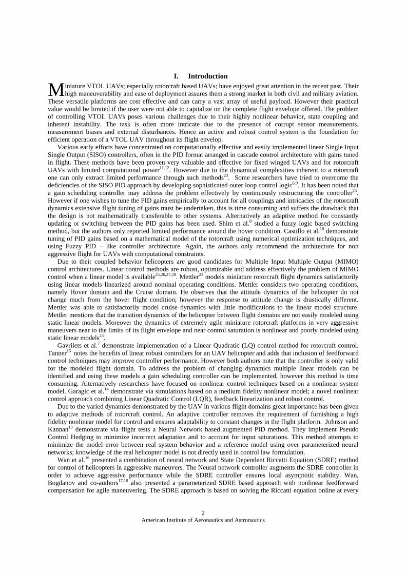
Figure 1: Unmanned Rotorcraft Technology Demonstrator ARTIS at DLR (German Aerospace Center)

The ARTIS is based on a commercially available miniature rotorcraft flight platform that is often used for

acrobatic flight by miniature helicopter pilots. The baseline vehicle is a modified Benda Genesis 1800 helicopter. Fully instrumented, the ARTIS UAV can carry up to 2kg of payload. Due to the extreme maneuverability and a very high thrust-to-weight ratio of the flight platform, the instrumented UAV is able to fly even the most dynamic and aggressive maneuvers. A multi-sensor navigation system based on off the shelf sensors has been developed for ARTIS which provides optimized navigation solutions using sensor fusion techniques. To facilitate the addition of extra hardware, the ARTIS UAV features a modular avionics subsystem that allows for easy reconfiguration and upgrades. Detailed information on the avionics suite can be found in reference 2 and 3.


4

III. Simulation Environment A comprehensive flight simulation setup is available at DLR for testing and evaluating flight and mission

systems for miniature rotorcraft UAVs. Currently three independent simulators are available in increasing level of fidelity to facilitate various stages of the development and prototyping process. The lowest fidelity simulation environment uses the non real-time MATLAB environment based on a windows platform and is network centric to facilitate rapid development. When an algorithm has been adequately verified it can be tested on the more comprehensive model based Software in the Loop (SITL) simulator. This simulator includes comprehensive model of the sensors, servos, time delays and external disturbances. The highest fidelity simulator is a real time Hardware in the Loop (HITL) simulator which interacts directly with the on board hardware in real-time. Only after rigorous verification on the HITL simulator is an algorithm or a mission system is prototyped for flight testing. Figure 2 gives a schematic overview of the Hardware in the loop simulation environment.

Figure 2, Hardware in the Loop Simulation Environment

The core simulation environment consists of a nonlinear model for miniature helicopter dynamics, sensor suite

emulation complete with noise emulation and simulation of external disturbances. The simulation model is based on a real-time computer. In simulation of autonomous flight the onboard flight computer is actively involved and hosts autonomy centric systems such as the control system, the Guidance and Navigation system, the obstacle detection and avoidance system etc. The mission environment is simulated on a real-time computer interfaced with an in-house developed simulation environment connected to multiple graphical displays. A cockpit emulator is also available which offers an intuitive interface using simulated flight instruments. The simulation can be setup for trajectory following, velocity following or attitude following modes. The user can interact with the simulator by using the remote control to directly control the bare dynamics of the helicopter or with a joystick in the “Easy handling mode”, where the dynamics are decoupled and stabilized using a control system.

IV. Controller Architecture Linear control techniques present robust and optimal tools for handling MIMO control problems. A large portion

of the dynamics of a miniature helicopter may be satisfactorily modeled by multiple linear models linearized around nominal operating conditions23,22,1. Some of the most common operating conditions are the Hover domain and the Cruise or Forward Flight domains linearized around a particular velocity. The attitude dynamics of the helicopter change only marginally from the core hover flight condition; however the response of the helicopter to changes in attitude is drastically different as the helicopter leaves the hover domain‡. Moreover the transitional dynamics between the domains are poorly modeled using static linear models as aerodynamic derivatives which are functions of velocity may vary constantly through the transition.

In the presented approach we aim to constantly update sufficient linear representation of the rotorcraft dynamics by identifying changing parameters online. Using the updated model new control gains are then calculated at each discrete time step. The online parameter identification accounts for changing parameters as the rotorcraft transits between flight domains and any initial parameter uncertainties. The trim values of the rotorcraft inputs are also estimated online and used for augmenting the controller input.

The rotorcraft dynamic model to be identified online may contain states that are not measurable (Unobserved states); hence a state estimation algorithm is used. Moreover the measurement data may contain noise and biases; these are accounted for in the design of the state filter. To address the combined problem of state and parameter

‡Mettler 0 shows that one could model both the hover and the cruise domains with minimal changes to the linear model structure although the derivatives will have different values in respective domains.


5

estimation in presence of measurement noise and biases we employ the Extended Kalman Filter (EKF) 4, 29 The EKF technique of parameter identification is well proven for such problems4, 5, 19.

The control architecture is implemented in real-time on an embedded processor; hence discrete formulation of the control law is used. The control effort at each discrete time step is summarized as follows,

1. Online Parameter Identification: Tune the online representation of parameterized rotorcraft dynamics by

estimating critical changing derivatives. Estimate the unobserved states of the system. 2. Active Control: Calculate new control gains based on the updated model. 3. Addition of trim: Use estimated trim values as Feed-forward inputs.

A. Identification Model In order to implement proven linear control techniques we choose a linear model as the model whose parameters

will be identified online. The continuous, parameter dependent, linear state space model for the rotorcraft dynamics is represented in Eq. (1).

ztxCy

xtxutuBtxAtx

C

trimBA

Δ+==Δ++=

)()()(),)()(()()()( 00

βββ

(1)

Where the system matrix A, the input matrix B and the measurement matrix C are functions of parameters to be identified β and [ ]CBA ββββ ;;= . Extended states Δutrim and zΔ represent the respective input and measurement biases to be identified. The state vector x consists of u, v and w which are the rotorcraft velocities in body x, y and z axes respectively, p, q and r which are the rotorcraft angular rates around the body x, y and z axes respectively. φ and θ which are the Euler angles as well as a and b which are respectively rotorcraft internal states for longitudinal and lateral rotor flapping angles. Sensor measurements are available for all the velocities, angular rates and Euler angles, however they may contain noise and sensor biases. The internal states a and b are not measured and must be estimated. It is important to note that the parameters as well as the trim and output bias values are not constant rather are functions of time. For linear representation of rotorcraft systems the measurement matrix C usually equates measurements directly to states, in this case the estimation problem is simplified as the number of parameters to be estimated is reduced. For the presented control architecture to hold the rotorcraft A,B and C matrices must be both controllable and observable.

B. Online Parameter Identification The extended Kalman filter is a recursive algorithm that uses the measured output and the known input, together

with the assumed system and output models as well as the assumed process and measurement noise statistics, to produce an estimate of the states and the estimation error covariance19. The EKF technique handles parameter estimation indirectly by artificially defining the unknown system parameters as state variables; this renders the estimation problem effectively nonlinear. The EKF approximates the nonlinear filtering problem by linearizing at each time step around the last best estimate of the nonlinear process as soon as it becomes available. In this way the linear representation is always valid for the current flight condition and large initial condition errors do not propagate. The discrete case EKF algorithm for estimating parameters of a continuous nonlinear representation of rotorcraft dynamics is presented.

The rotorcraft dynamics are represented in generic continuous state space form along with the discrete measurement equation in Eq. (2),

NkkGvkykztutxgty

xtxtFwtutxftx

,....1),()()(]),(),([)(

)(),(]),(),([)( 00

=+==

=+=ββ

(2)

Where x is the state vector having initial value x0 at time t0, u is the input vector, y is the observation vector, Θ is the vector of unknown system parameters, f and g are the general nonlinear real-valued functions, z is the measurement vector sampled at N discrete time steps having a fixed sampling time of tΔ and k is the discrete time index. The measurement noise vector ν is assumed to be sequence of independent zero mean white Gaussian noise.


6

The matrices F and G represent the additive state and measurement noise matrices and are considered to be time invariant.

The unknown parameter vector Θ consists of system parameters β , the measurement biases zΔ and the trim estimates formulated as input biases uΔ § and is represented in Eq. (3).

{ }TTTT uz ΔΔ=Θ ;;β (3)

We consider the constant system parameters Θ as output of an auxiliary dynamic system presented in Eq. (4),

0=Θ (4)

The augmented state vector is then defined in Eq. (5) as:

⎥⎦

⎤⎢⎣

⎡Θ

=x

xa (5)

The extended system is represented in Eq. (6) as:

)()()()](),([)(

0)(

000

0]),(),([

)()](),([)(

kGvkykztutxgty

twFtutxftWFtutxftx

aa

aaaaa

+==

⎥⎦

⎤⎢⎣

⎡⎥⎦

⎤⎢⎣

⎡+⎥

⎦

⎤⎢⎣

⎡=

+=

β (6)

Where the subscript “a” denotes the augmented variables. For the above augmented system the EKF consisting of an extrapolation (prediction) and an update are summarized below4,29. In what follows we use the notation “tilde” (~) and “hat” (^) to denote the predicted and corrected variables respectively.

Extrapolation:

T

aaTaaaa

aa

kt

ktaaaa

FFtkkPkkP

kukxgky

dtkutxfkxkx

.)()1(ˆ)()(~)](),(~[)(~

)](),([)1(ˆ)(~)(

)1(

Δ+Φ−Φ≈

=

+−= ∫−

(7)

Where tA

aae Δ=Φ denotes the discrete time state transition matrix from the augmented system with,

)1(ˆ)1(ˆ00

)(−=−=

⎥⎥

⎦

⎤

⎢⎢

⎣

⎡Θ∂∂

∂∂

==∂∂

kxxkxx

a

aaaa

fxf

a

akAxf

(8)

§ It may not be possible to estimate all the components of zΔ and uΔ since they could be linearly dependent or highly correlated4.


7

Eq. (8) denotes the linearization process for the state matrix. The linearization can be carried out using a numerical implementation of the central difference formula around the last best state estimate at each discrete time step as in Eq. (11).

Update:

)()()]()()[(~)]()([

)(~)]()([)(ˆ)](~)()[()(~)(ˆ

])()(~)()[()(~)( 1

kKGGkKkCkKIkPkCkKI

kPkCkKIkP

kykzkKkxkxGGkCkPkCkCkPkK

Ta

Ta

Taaaaa

aaaa

aaa

TTaaa

Taaa

+−−=

−=

−+=+= −

(9)

Where Ca(k) is the linearized measurement function as represented in Eq. (10), as before the linearization can be carried out using a numerical implementation of the central difference formula, Eq. (11).

)(~

)(~

)(kxx

kxx

aaa

aa

gxg

a

akCxg

==

⎥⎦⎤

⎢⎣⎡

Θ∂∂

∂∂

==∂∂

(10)

The Runge-Kutta algorithm can be used for integration in Eq. (7), the propagation of the covariance matrix P in Eq. (9) is approximated for a small tΔ . The state transition matrix aΦ can be approximated using Padè approximation21 or Taylor series expansion.

The gradients in Eq. (8) and Eq. (10) can be approximated using the central difference formula for a small perturbation jxδ as follows 0 :

[ ] [ ]

[ ] [ ])(~

)1(ˆ

)(2),(,)()(),(,)()(

)(

)(2),(,)()(),(,)()(

)(

kxxj

jji

jji

ij

kxxj

jji

jji

ij

kxkuekxkxgkuekxkxg

kC

kxkuekxkxfkuekxkxf

kA

=

−=

−−+≈

−−+≈

δβδβδ

δβδβδ

(11)

The vector ej in Eq. (11) is a vector with unit jth value and the rest zero. In the above representation the Pa(0) represents the confidence in the initial state estimates and must be specified

a priori. In the absence of any a priori knowledge of the parameter values it is common to assume high values for the Pa(0) matrix4. The value of FFT and GGT i.e. the process and measurement noise covariance matrices must also be specified a priory. The measurement noise covariance matrix GGT can be calibrated using laboratory measurements of sensors to ensure good noise filtering. The process noise covariance matrix FFT is however more difficult to determine. We observed good results via manual tuning offline, against varied flight data; starting from low positive values for the FFT matrix is recommended. We have also observed that the parameter estimation is relatively insensitive to the values of the covariance matrices. The problem of estimating noise statistics or “Adaptive Filtering”30 has not been addressed in this paper.

C. Active Riccatti Control Using the current estimates of the parameters from the corrected augmented state vector x the continuous time

linear representation of the helicopter dynamics is updated. The updated model is then discretized for control purposes, the discrete representation is presented in Eq.(12) as:

kk

kdkdk

CxyuBxAx

=+=+1 (12)


8

Where Ad is the discrete time state transition matrix, Bd is the discrete time input matrix and C is the linear observations matrix. These matrices are obtained from their continuous counterparts as in Eq. (13):

BdeB

eAt

o

Ad

tAd

ˆˆ

ˆ

⎟⎟⎠

⎞⎜⎜⎝

⎛=

=

∫Δ

=

Δ

τ

τ τ (13)

Where A and B are the updated continuous state and input matrices from Eq. (1), the update process is achieved by updating the parameters of the A and B matrices by their counterparts in the parameter vector Θ . This relationship is made clear in Eq. (14):

( ) ( )

( ) ( )a

a

xBBB

andxAAA

ˆˆ

ˆˆ

=Θ=

=Θ= (14)

The LQR approach25,26,27,28 is used to control of linear MIMO systems is a proven approach known for its robustness and optimality. Using the newly identified parameters of the reference linear model the LQ gains are calculated by solving the discrete time Riccatti equation online at every discrete time step. The LQR cost function that is to be minimized is specified in Eq. (15) as:

( )0

( ) T Tk k k k

kj u x Qx u Ru

∞

=

= +∑ (15)

Where N is the time horizon, the first term containing the containing the Qf matrix measures the final state deviation, the first term in the summation containing the Q matrix measures the state deviation and the second term containing the R matrix measures the actuator authority. Using the Q and the R matrices one can set relative weights for state deviation and actuator deflection. The solution to the LQR problem is achieved by propagating the Riccatti solution matrix S:

Prediction:

QASAS dkTdk += −1

ˆ~ (16)

LQR gain calculation:

dkTddk

Tdk ASBRBSBG ~)~( 1−+= (17)

Update:

[ ]kTddk

Tddkkk SBRBSBBSSS ~)~(~~ˆ 1−+−= (18)

In the above numerical solution method using the predictive – recursive form the solution is seen to converge rapidly within few time steps. Alternatively one could use the recursive dynamic programming approach and run the LQR algorithm backwards in time for predefined number of iterations N (imposing a constraint on Sk=N)at each discrete time step. If sufficient backwards integration is done converged solution will be available at each time step,


9

this approach is however, computationally intensive. We have observed that the predictive – recursive approach as illustrated in Eq. (16) to Eq. (18); approximates the optimal solution closely, alleviates the computational load on the processor, and exhibits rapid convergence hence is preferable for real-time applications.

The stabilizing control input can then be calculated using the negative observed state feedback scheme:

( )kcommandkk xxGu −−= ˆ (19)

Where kx is the last best state estimate and kcommandx is the commanded state vector at discrete time step k. kx

is extracted from the last corrected estimate of the augmented state vector ax of Eq.(5). Initial value of the S matrix can be set to identity or equal to that of the Q matrix. The LQR weighing matrices Q and R can be tuned to address control system specifications.

D. Addition of Trim and outer loop control Linear perturbed state models are linearized around steady state trim values. These trim values are identified

using the EKF as input biases as shown in Eq. (1). The identified bias values are added directly to the control input, this effectively resets the zero value of the control input resulting in the control input having zero value at the trim condition and positive or negative values around the trim condition. This approach accounts for changes in trim due to external disturbances such as gusts, ground effect etc.

Position control is achieved by an outerloop controller that converts position commands to velocity commands u, v and w. In similar fashion heading control is achieved by an outerloop controller that converts heading commands to yaw rate r. The implemented MIMO architecture then follows the commands by minimizing the error between the commanded and actual states.

V. Simulation Results The results of SITL and HITL simulations are now presented. We begin with results of parameter identification

using the EKF against real flight data, progressing onwards to results of simulation in velocity tracking and trajectory tracking modes with the presented control architecture.

A. EKF as an independent parameter estimator In the presented control architecture the EKF addresses the combined problem of state and parameter estimation.

For the purpose of assessing the EKF as an online parameter identification tool, the EKF was tested as an independent parameter identifier. Results of one such parameter identification run in hover domain against real flight data are presented in this subsection. The flight data contains considerable amount of noise and biases in measurements. Trim values are roughly known based on pilot feedback. The parameters whose convergence will be observed are,

Lb : Effect of lateral rotor flapping angle on the lateral moment. Ma : Effect of longitudinal rotor flapping angle on longitudinal moment. Alon : Effect of longitudinal input on lateral rotor flapping angle. Blat : Effect of lateral input on longitudinal rotor flapping angle. These aerodynamic derivatives have strong influence on rotorcraft pitch and roll rates, the first two are

parameters of the state matrix A, whereas the last two are parameters of the input matrix B. The presented identification run uses flight data from lateral and longitudinal input sweep maneuvers. In1 we have identified an extended linear model of the ARTIS VTOL UAV in hover domain; the values of the parameters identified therein are considered as the nominal values for hover domain. Our results suggest that in the vicinity of the hover domain parameter values lie within 15% of the nominal values.

The results of the identification run are presented in section I of the appendix. Figure 3, Estimation of velocities with EKF and Figure 4, Estimation of angular rates with EKF show the noisy measurements and the EKF state estimates for the rotorcraft velocities and angular rates respectively. Figure 5, Parameter estimation for real data shows the track of the parameter estimated by the EKF. The dependence of the parameter convergence on rich data is clearly visible when one observes the correlation between the input sweep maneuvers and parameter convergence.


10

The fastest movement in parameters is seen in the first 50 seconds of estimation, where the high initial uncertainty forces the parameters to converge swiftly near to their expected values. In the rest of the estimation run the EKF then fine tunes the parameters to match the current flight state. The quick initial convergence in presence of noisy data asserts the suitability of the EKF in online applications.

B. Velocity control in presence of parameter uncertainty Simulation results for velocity tracking control are presented in this subsection. To demonstrate the inner loop

negative estimated state feedback architecture we command three consecutive velocity steps in the z, x and y direction respectively. Only noisy sensor measurements are available for control, the controller has no a priori information about the trim and a parameter uncertainty is simulated by initializing the parameters randomly within 30 percent of their nominal values around hover domain. The parameters observed are,

θX : Effect of pitch angle θ on longitudinal velocity u

φY : Effect of roll angle φ on lateral velocity v Alon : Effect of longitudinal input on longitudinal flapping angle. Blat : Effect of lateral input on lateral flapping angle. The first two parameters relate the effect of change in rotorcraft attitude angles to the velocities, their values can

be expressed as in Eq. (20). The nominal values linearized around hover domain are found by assuming small θ and φ and approximating the values to –g and +g respectively. The last two parameters are parameters of the input matrix relating the cyclic inputs to roll and pitch motion:

φφθ

θθ

φ

θ

sincos

sin

gY

gX

=

−= (20)

To asses the presented control architecture we simulate a parameter uncertainty by initializing θX and φY with more than 80% error and randomly assigning an error of up to 30% for rest of the parameters. The parameters are estimated online using the EKF which updates an instantaneously linearized representation of system dynamics. Using the updated mathematical model new LQ gains are calculated at each discrete time step which are then used for control in estimated state feedback architecture and the control input are augmented with trim estimates.

The results of the simulation are presented in section II of the Appendix. Figure 6, Velocity command tracking and estimation shows the velocity tracking along with the estimated states. Figure 7, Angular rate estimation shows the EKF filtering of the angular rates from noisy data. Figure 8, Online parameter estimation using EKF and Figure 9, Online trim estimation using EKF show the tracks of online aerodynamic derivatives and trim estimates. Excellent output filtering and command following is seen. The parameters converge quickly within acceptable margins as soon as excitation in u and v are available which in this case is presented by the coupling effects of vertical velocity on the lateral and longitudinal velocities. The quick convergence of the parameters ensures control even in presence of initial parameter uncertainty. The effect of converged parameters on the control accuracy is clearly seen if one observes Figure 6 and Figure 8 in conjunction. The step inputs present rich data which the EKF uses for further fine tuning of the parameter estimates, hence the state regulation and command following after the execution of the step inputs is seen to improve compared to that of before. The results clearly indicate quick and successful controller adaptation to initial parameter uncertainties. The trim estimates are seen to vary slightly depending on the states indicating successful trim estimation and controller augmentation.

C. Trajectory tracking control in presence of external disturbance Simulation results for trajectory and heading tracking control are discussed in this subsection. The results for

trajectory and heading tracking control are presented in section III of the appendix. The desired trajectory consists of a climb from 0m to 10m, followed by a three dimensional rectangle, and a sideward flight of 100 meters. This is followed by a circular loiter trajectory around the end point. Finally the rotorcraft aligns itself with the end point and descents to 0m. . Only noisy sensor measurements are available, parameter uncertainty is simulated by initializing


11

the parameters randomly within 30 percent of their nominal values. Trim values are assumed unknown and estimated online. An external disturbance forcing an acceleration of 2m/s2 in inertial x direction and 3m/s2 in inertial y direction onto the helicopter is applied after 50 seconds of flight duration, the disturbance then continues throughout the remainder of the flight. Figure 10, Trajectory tracking in presence of external disturbance shows the performance of the presented control architecture in trajectory following flight. The inset in figure 10 zooms on to the circular loiter trajectory. Figure 11, Altitude tracking in presence of external disturbances shows the performance in altitude tracking for the followed trajectory. Figure 12 and Figure 13 show the controller response in terms of velocities and angular rates in body frame respectively. In Figure 14, Online trim estimates it is seen that the after the application of the external disturbance the EKF estimates different trim values for the collective input from that of the expected steady state trim value. The change in trim values is explained as follows, the controller tilts the rotorcraft in the direction of the disturbance so as to counteract the external forces. The resulting tilting of the rotor lift vector forces an increase in the collective trim input to maintain altitude. The control system is seen to responds by increasing the collective trim in order to maintain altitude and position accuracy. Figure 15 Trajectory tracking without adaptive trim shows the performance without adaptive trim, it is clearly seen that without the addition of adaptive trim the UAV drifts off the course. Excellent trajectory tracking capability of the presented controller architecture in presence of noisy sensor data, parameter uncertainty and external disturbances indicates robust and accurate control.

Figure 16, Heading command tracking shows the performance of the presented control architecture against yaw angle commands. Heading commands are converted to yaw rate commands by an outer loop controller. The presented EKF – LQR control architecture is then used to ensure command following in presence of noisy sensor data and parameter uncertainty.

VI. Conclusion In this paper we have demonstrated an adaptive method for control of VTOL UAVs in presence of parameter

uncertainty, noisy sensor measurements and external disturbances. An Extended Kalman Filter was used for the combined problem of state and parameter estimation, using the updated parameters control was achieved by solving the Riccatti equation online. The presented control architecture inherits the robust performance of the LQR method and the good state estimation properties of the EKF. Parameter identification runs using the EKF against real flight data indicated that the parameter convergence is principally dependent only on the richness of the data and asserted the suitability of the EKF for online control applications. The presented control architecture was tested in real-time simulations for performance in velocity following and trajectory following control; the positive results indicated the feasibility of this approach. The main benefits of the presented control architecture are: (i). Incorporation of online parameter identification technique relaxes the constraints on the accuracy of the flight dynamics model. (ii). Use of parameter dependent robust control methods ensure that the need for manual tuning of multiple gains is minimized. (iii). Inherent linearization and the emphases on the well proven robust MIMO control techniques render the control architecture reliable. (iv). Incorporation of the EKF for state estimation and filtering purposes ensures that good performance is achieved even in the presence of considerable sensor noise or biases. (v). The incorporated LQR method of linear MIMO control allows via the use of the R matrix control over the amount of control input used and via the use of the Q matrix control over the stability of the system zero dynamics. This flexibility ensures that the control law can be better tuned to meet performance requirements. (vi). Online estimation of trim ensures validity of the linear model and handles any in-flight changes in trim conditions.


12

Appendix

I. Results of EKF used as a parameter identification tool against real data

9750 9760 9770 9780 9790 9800 9810 9820

-2

0

2

Estimation of velocities

u m

/s

9750 9760 9770 9780 9790 9800 9810 9820

-2

0

2

v m

/s

9750 9760 9770 9780 9790 9800 9810 9820

-2

0

2

w m

/s

time in seconds

Nav MeasurementsEKF State estimates

Figure 3, Estimation of velocities with EKF

9750 9760 9770 9780 9790 9800 9810 9820-2

-1

0

1

2Estimation of angular rates

p ra

d/s

9750 9760 9770 9780 9790 9800 9810 9820-2

-1

0

1

2

q ra

d/s

9750 9760 9770 9780 9790 9800 9810 9820-2

-1

0

1

2

r rad

/s

time in seconds


Figure 4, Estimation of angular rates with EKF

9750 9760 9770 9780 9790 9800 9810 98200

200

400

600

Parameter estimates

Lb

9750 9760 9770 9780 9790 9800 9810 98200

100

200

Ma

9750 9760 9770 9780 9790 9800 9810 9820

-4

-2

0

Alo

n

9750 9760 9770 9780 9790 9800 9810 9820

-4

-2

0

Bla

t

time in seconds

Expected parameter valueEKF estimate of parameter value15 percent parameter uncertanity bound

Figure 5, Parameter estimation for real data

II. Simulation results, Velocity steps

5 10 15 20 25 30 35-4

-2

0

2

4Velocity command tracking using estimted states in presence of parameter uncertanity

u m

/s

5 10 15 20 25 30 35-4

-2

0

2

4

v m

/s

5 10 15 20 25 30 35-4

-2

0

2

4

w m

/s

time in seconds

Nav MeasurementsEKF State estimatesVelocity Commands

Figure 6, Velocity command tracking and estimation

5 10 15 20 25 30 35-2

-1

0

1


p ra

d/s

5 10 15 20 25 30 35-2

-1

0

1

2

q ra

d/s

5 10 15 20 25 30 35-2

-1

0

1

2

r rad

/s

time in seconds


Figure 7, Angular rate estimation

5 10 15 20 25 30 35

-15

-10

-5

0Parameter estimates

Xth

eta

5 10 15 20 25 30 350

5

10

15

Yph

i

5 10 15 20 25 30 35

-4

-2

0

Alo

n

5 10 15 20 25 30 35

-4

-2

0

Bla

t

time in seconds

Expected parameter valueEKF estimate of parameter value15 percent parameter uncertanity bound

Figure 8, Online parameter estimation using EKF


13

5 10 15 20 25 30 35-0.5

0

0.5Trim estimates velocity steps

late

ral %

5 10 15 20 25 30 35-0.5

0

0.5

long

itudi

nal %

5 10 15 20 25 30 35-0.5

0

0.5

peda

l %

5 10 15 20 25 30 35-0.5

0

0.5

colle

ctiv

e %

time in seconds

Approximate expected trim valueEKF trim value estimates

Figure 9, Online trim estimation using EKF

III. Simulation results, Trajectory tracking

-100 -50 0 50 100-50

0

50

100

150

X, m

Y, m

Trajectory tracking

CommandFollowed

Figure 10, Trajectory tracking in presence of external disturbance

50 100 150 200 250 3000

5

10

15

20

25

30

Time, s

Z, m

Altitude tracking

CommandFollowed

Figure 11, Altitude tracking in presence of external

disturbances

50 100 150 200 250 300-4

-2

0

2

4Velocity command tracking using estimted states in presence of parameter uncertanity

u m

/s

50 100 150 200 250 300-4

-2

0

2

4

v m

/s

50 100 150 200 250 300-4

-2

0

2

4

w m

/s

time in seconds

Nav MeasurementsEKF State estimatesVelocity Commands

Figure 12, Velocity commands, tracking and estimation

50 100 150 200 250 300-2

-1

0

1


p ra

d/s

50 100 150 200 250 300-2

-1

0

1

2

q ra

d/s

50 100 150 200 250 300-2

-1

0

1

2

r rad

/s

time in seconds


Figure 13, Filtering of angular rates

50 100 150 200 250 300

-0.2

0

0.2

Trim estimates

late

ral %

50 100 150 200 250 300

-0.2

0

0.2

long

itudi

nal %

50 100 150 200 250 300

-0.2

0

0.2

peda

l %

50 100 150 200 250 300

-0.2

0

0.2

colle

ctiv

e %

time in seconds

Approximate expected trim valueEKF trim value estimates

Figure 14, Online trim estimates

-10 -5 0 5 10 15 20 25 30 3580

85

90

95

100

105

110

115

X, m

Y, m

Trajectory tracking


14

-100 -50 0 50 100-50

0

50

100

150

X, m

Y, m

Trajectory tracking without using feedforward trim

CommandFollowed

Figure 15 Trajectory tracking without adaptive trim

20 40 60 80 100 120 140

-0.5

0

0.5

1

1.5

2

2.5

3

psi,

rad

Time, s

Yaw angle tracking

State EstimatesCommand

Figure 16, Heading command tracking

Acknowledgments The authors would like to thank Dr. Frank Thielecke and Dr. Ravindra Jategoankar and for providing guidance

and support in the preparation of this work. The authors would also like to thank Joerg Dittrich, Lucas Heitzmann Gabrielli and the ARTIS team for their continuing support.

References 1Lorenz S., Chowdhary G., “System Identification for a Miniature Rotorcraft, Preliminary Results”, AHS 61st forum,

Grapevine TX June, 2005 2Dittirich J., Bernartz A., Thielecke F. “Intelligent Systems Research using a Small Autonomous Rotorcraft Testbed”, 2nd

AIAA “Unmanned Unlimited”, San Diego CA, September 2003. 3Dittiirch J., Thielecke F., Schwaneck H., “Unmanned Rotorcraft Testbed ARTIS: Challenges in Autonomous Control and

Teaming”, AHS 60th Annual Forum, Baltimore MD, 2004. 4Jategaonkar R., Plaetenschke E., „Estimation of Aircraft Parameters using Filter Error Methods and Extended Kalman

Filter“, DFVLR Institute für Flugmechanik Braunschweig, Germany 1988. 5Jategaonkar R., Bassappa, “Evaluation of Recursive Methods for Aircraft Parameter Estimation”, AIAA paper no. 2004-

5063 Providence, RI, 2004 . 6Kim Jin H., Shim David H., “Flight Control System for Aerial Robots, Algorithms and Experiminets”, Elsevier Scubces Ltd.

2003. 7Gavrilets V, Martinos I. Mettler B., Feron E., “Control Logic for Automated Aerobatic Flight of a Miniature Helicopter”,

Monterrey CA AIAA GNC 2002 . 8Shim H., Koo T. J., Hoffmann F., Sastry S., “A comprehencsive Study of Control Design for an Autonomous Helicopter”,

IEEE conference on Decision and Control, Dec 1999. 9Harbicks K., Montgomery F., Sukhatme G., “Planar Spline Following for an Autonomous Helicopter”, Journal of Advanced

Computational Intelligence and Intelligent Informatics, Vol.8, No.3 pp. 237-242, 2004 10Castillo C., Alvis W., Castillo-Effen M., Valavanis K., Moreno W., “Small Scale Helicopter Analysis and Controller

Design for Non-Aggressive Flights”, 58th AHS Forum, Montreal, 2002. 11Castillo P, Dzul A., Lozanno R., “Real Time Stabilization and Tracking of a Four – Rotor Mini Rotorcraft”, IEEE

Transactions on Control Systems Technology, VOL. 12, No. 4, July 2004. 12Roberts J., Corke P., Buskey G., “Low Cost Flight Control System for a Small Autonomous Helicopter”,ARAA 2002. 13Johnson E., Kannan S., “Adaptive Flight Control for an Autonomous Unmanned Helicopter”, AIAA GNC 2002, Monterrey

CA 2002. 14Garagic D., Boskovic J., Mehra R. “Robust Nonlinear Fault-Tolerant Control of a Small-Scale Helicopter”, AHS 60th

forum, Baltimore, MD, June 2004. 15Tanner O., “Modeling, Identification, and Control of Autonomous Helicopters”, PhD Dissertation to the Swiss Federal

Institute of Technology, Zurich, Switzerland 2003. 16Wan E, Bogdanov A., Kieburtz R., Baptista A., Carlsson M., Zhang Y., Zulauf M., “Model Predictive Neural Control for

Aggressive Helicopter Maneuvers”, in Software Enabled Control: Information Technologies for Dynamic Systems, IEEE press, 2003.


15

17Bogdanov A., Carlsson M., Harvey G., Hunt J., Kieburtz D., Van Der Merwe R., Wan E. “State Dependent Riccatti Equation Control of a Small Unmanned Helicopter”, AIAA GNC Austin TX , 2003.

18Bogdanov A., Wan E., “SDRE Control with Nonlinear Feedforward Compensation for a Small Unmanned Helicopter”, Second AIAA “Unmanned Unlimited” Conference San Diego CA, 2003.

19Gracfa-Velo J., Walker B. K., “Aerodynamic Parameter Estimation for High Performance Aircraft using Extended Filters”, AIAA-95-3500-CP, , 1995.

20Stein G., Athans M., “The LQG/LTR Procedure for Multivariable Feedback Control Design”, IEEE log no. 8612203, 1986

21Baker G. A. Jr., “The Theory and Application of The Pade Approximant Method”, In Advances in Theoretical Physics, Vol. 1 (Ed. K. A. Brueckner). New York: Academic Press, pp. 1-58, 1965.

22Mettler B., Tischler M., Kanade T., “System Identification of Small-Size Unmanned Helicopter Dynamics”, AHS 55th Forum, Montreal Quebec Canada 1999.

23Mettler B., “Modeling Identification and Characteristics of Miniature Rotorcrafts”, Kluwer Academic Publishers 2003 USA.

24Padfield G. D., “Helicopter Flight Dynamics: The theory and application of flying qualities and simulation modeling”, AIAA education series, USA,1996

25Levine William S (Editor). “The Control Handbook”, CRC press, London, 1996. 26Ogata Katushito, “Modern Control Engineering”, Third Edition, Prentice Hall, New Jersey, 2002. 27Graham G. Graebe S., Salgado M. “Control System Design”, Prentice Hall, New Jersey, 2001 28Bryson A. Jr., Ho Yo-Chin, “Applied Optimal Control”, Hemisphere Publishing Corp. USA, 1975. 29Grewal M., Andrews A., “Kalman Filtering Theory and Practice using MATLAB”, Second Edition, John Wiley and Sons,

USA 2001 30Gelb A. “Applied Optimal Estimation”, MIT press, Massachusetts USA 1974

control of a vtol uav via online parameter estimation · control of a vtol uav via online parameter...

Documents