Intelligent Control of a Ducted-Fan VTOL UAV with

Conventional Control Surfaces

A thesis submitted in fulfilment of the requirements for the degree of

Doctor of Philosophy

Zamri Omar

M.Eng.

School of Aerospace, Mechanical, and Manufacturing Engineering

College of Science, Engineering and Health

RMIT University

March 2010

i

DECLARATION

I certify that except where due acknowledgement has been made, the work is that

of the author alone; the work has not been submitted previously, in whole or in part, to

qualify for any other academic award; the content of the thesis is the result of work which

has been carried out since the official commencement date of the approved research program;

any editorial work, paid or unpaid, carried out by a third party is acknowledged; and, ethics

procedures and guidelines have been followed.

Zamri Omar

6 October 2010

ii

ACKNOWLEDGMENTS

I would like to thank many people who have enabled me to conduct this research. First,

I am very grateful to my supervisors, Associate Professor Cees Bil and Dr. Robin Hill for their

outstanding guidance, support, and patience all the way through. I would like express my

thankful to my sponsorship providers; Public Service Department of Malaysia and Ministry

of Higher Education Malaysia (Grant No: JPA(L)740414017077), and Universiti Tun Hussein

Onn Malaysia (Grant No: KUiTTHO.PP/S/10.14/09 Jld 3(73)) for granting me a continuous

financial support for this research and during my overseas stay. Thank you also to many staff

at RMIT University and Universiti Tun Hussein Onn Malaysia who have helped me in many

different ways. To my parents, my sincere thanks for their consistent love, support, and

prayers. A very special thanks is to my wife, Fazlinda, for her endless patience, love, and

support. To my son, Azim, and daughter, Rania, thanks for your patience too in allowing

your dad to do his work at home. Finally, my greatest gratitude is to The Almighty God,

that is Him who has made this thesis a reality.

iii

TABLE OF CONTENTS

Declaration ii

Acknowledgments iii

List of Figures x

List of Tables xv

Summary 1

Chapter 1: Introduction 2

1.1 Rationale . . . . . . . . . . . . . . . . . . . . . . . . . . . . . . . . . . . . . . 2

1.2 Problem Statement . . . . . . . . . . . . . . . . . . . . . . . . . . . . . . . . . 4

1.3 Scope and Limitations . . . . . . . . . . . . . . . . . . . . . . . . . . . . . . . 6

1.4 Thesis Outline . . . . . . . . . . . . . . . . . . . . . . . . . . . . . . . . . . . . 7

Chapter 2: Literature Review and Theoretical Background 8

2.1 Introduction . . . . . . . . . . . . . . . . . . . . . . . . . . . . . . . . . . . . . 8

2.2 Needs and Challenges for VTOL UAVs . . . . . . . . . . . . . . . . . . . . . . 8

2.3 Demands for Small Ducted-Fan UAVs . . . . . . . . . . . . . . . . . . . . . . . 11

2.4 Ducted-Fan VTOL UAV Configurations . . . . . . . . . . . . . . . . . . . . . 13

2.5 Challenges and Approaches to Autonomous Control of Ducted-Fan UAVs . . . 17

2.5.1 Conventional Flight Control System . . . . . . . . . . . . . . . . . . . . 19

2.5.2 Intelligent Flight Control System . . . . . . . . . . . . . . . . . . . . . 21

iv

2.6 Fuzzy Logic Theory . . . . . . . . . . . . . . . . . . . . . . . . . . . . . . . . . 25

2.6.1 Fuzzy Sets . . . . . . . . . . . . . . . . . . . . . . . . . . . . . . . . . . 26

2.6.2 Membership Functions and Logical Operators . . . . . . . . . . . . . . 29

2.6.3 Linguistic Variable and Hedges . . . . . . . . . . . . . . . . . . . . . . 32

2.6.4 Rule Base and Data Base . . . . . . . . . . . . . . . . . . . . . . . . . 34

2.6.5 Fuzzification, Fuzzy Inference, and Deffuzzification . . . . . . . . . . . 36

2.6.6 Scaling Factors, Tuning, and Evaluation . . . . . . . . . . . . . . . . . 43

2.7 Summary . . . . . . . . . . . . . . . . . . . . . . . . . . . . . . . . . . . . . . 44

Chapter 3: Configuration, Aerodynamic, and Propulsion 45

3.1 Introduction . . . . . . . . . . . . . . . . . . . . . . . . . . . . . . . . . . . . . 45

3.2 Vehicle Configuration . . . . . . . . . . . . . . . . . . . . . . . . . . . . . . . . 45

3.2.1 Design Considerations . . . . . . . . . . . . . . . . . . . . . . . . . . . 47

3.2.2 Geometrical Layout and Properties . . . . . . . . . . . . . . . . . . . . 48

3.2.3 Mass and Inertia Properties . . . . . . . . . . . . . . . . . . . . . . . . 51

3.2.4 Vehicle Specialty and Missions . . . . . . . . . . . . . . . . . . . . . . . 56

3.3 Aerodynamic . . . . . . . . . . . . . . . . . . . . . . . . . . . . . . . . . . . . 57

3.3.1 Aerodynamic Coefficients . . . . . . . . . . . . . . . . . . . . . . . . . 58

3.3.1.1 Drag Estimation . . . . . . . . . . . . . . . . . . . . . . . . . 64

3.3.1.2 Stators Design . . . . . . . . . . . . . . . . . . . . . . . . . . 67

3.3.1.3 Propeller Effects . . . . . . . . . . . . . . . . . . . . . . . . . 68

3.3.2 Control Surfaces Design . . . . . . . . . . . . . . . . . . . . . . . . . . 69

3.3.3 Control Surfaces Aerodynamic . . . . . . . . . . . . . . . . . . . . . . . 71

3.4 Propulsion . . . . . . . . . . . . . . . . . . . . . . . . . . . . . . . . . . . . . . 77

3.4.1 Power Estimation . . . . . . . . . . . . . . . . . . . . . . . . . . . . . . 77

3.4.2 The Thrust . . . . . . . . . . . . . . . . . . . . . . . . . . . . . . . . . 84

3.4.3 Model of Brushless D.C Motor . . . . . . . . . . . . . . . . . . . . . . . 89

v

3.5 Summary . . . . . . . . . . . . . . . . . . . . . . . . . . . . . . . . . . . . . . 92

Chapter 4: Vehicle dynamics 93

4.1 Introduction . . . . . . . . . . . . . . . . . . . . . . . . . . . . . . . . . . . . . 93

4.2 Axis Systems Definition . . . . . . . . . . . . . . . . . . . . . . . . . . . . . . 93

4.2.1 Body-Axis System . . . . . . . . . . . . . . . . . . . . . . . . . . . . . 93

4.2.2 Earth-Axis System . . . . . . . . . . . . . . . . . . . . . . . . . . . . . 94

4.2.3 Stability and Wind Axis Systems . . . . . . . . . . . . . . . . . . . . . 95

4.3 Equations of Motion . . . . . . . . . . . . . . . . . . . . . . . . . . . . . . . . 95

4.4 Aircraft Attitude and Position . . . . . . . . . . . . . . . . . . . . . . . . . . . 99

4.4.1 Axis Transformation . . . . . . . . . . . . . . . . . . . . . . . . . . . . 101

4.4.2 Kinematic Equations . . . . . . . . . . . . . . . . . . . . . . . . . . . . 104

4.4.3 Navigational Equations . . . . . . . . . . . . . . . . . . . . . . . . . . . 106

4.4.4 Vertical Euler Angles Representation . . . . . . . . . . . . . . . . . . . 107

4.4.5 Quaternion Representation . . . . . . . . . . . . . . . . . . . . . . . . . 110

4.5 Force and Moment . . . . . . . . . . . . . . . . . . . . . . . . . . . . . . . . . 111

4.6 Numerical Solution . . . . . . . . . . . . . . . . . . . . . . . . . . . . . . . . . 112

4.7 Summary . . . . . . . . . . . . . . . . . . . . . . . . . . . . . . . . . . . . . . 112

Chapter 5: Flight Control System Design 114

5.1 Introduction . . . . . . . . . . . . . . . . . . . . . . . . . . . . . . . . . . . . . 114

5.2 General Overview of Flight Phases and Control . . . . . . . . . . . . . . . . . 114

5.3 Control Design Approach . . . . . . . . . . . . . . . . . . . . . . . . . . . . . . 120

5.3.1 The Guidance Loop . . . . . . . . . . . . . . . . . . . . . . . . . . . . . 123

5.3.2 The Control Loop . . . . . . . . . . . . . . . . . . . . . . . . . . . . . . 124

5.3.3 Control Design Steps . . . . . . . . . . . . . . . . . . . . . . . . . . . . 125

5.3.4 Dominant Controller . . . . . . . . . . . . . . . . . . . . . . . . . . . . 127

vi

5.3.5 Synthesis of Fuzzy Rules . . . . . . . . . . . . . . . . . . . . . . . . . . 129

5.3.6 Properties of the FLC . . . . . . . . . . . . . . . . . . . . . . . . . . . 134

5.3.6.1 Input and Output Variables . . . . . . . . . . . . . . . . . . . 134

5.3.6.2 Fuzzy Sets, and Membership Functions . . . . . . . . . . . . . 135

5.3.6.3 Universe of Discourse, and Scaling Factors . . . . . . . . . . . 136

5.3.6.4 The Rules . . . . . . . . . . . . . . . . . . . . . . . . . . . . . 137

5.3.7 Computational Tools . . . . . . . . . . . . . . . . . . . . . . . . . . . . 137

5.4 Vertical Flight Controller . . . . . . . . . . . . . . . . . . . . . . . . . . . . . . 138

5.4.1 Vertical Flight Guidance . . . . . . . . . . . . . . . . . . . . . . . . . . 141

5.4.1.1 Low-Speed Tilted Flight Guidance . . . . . . . . . . . . . . . 143

5.4.1.2 Ascend, Descend, and Pirouette Flight Guidance . . . . . . . 148

5.4.2 Vertical Flight Control . . . . . . . . . . . . . . . . . . . . . . . . . . . 149

5.4.2.1 Low-Speed Tilted Flight Control . . . . . . . . . . . . . . . . 151

5.4.2.2 Ascend and Descend Flight Control . . . . . . . . . . . . . . . 154

5.4.2.3 Pirouette Control . . . . . . . . . . . . . . . . . . . . . . . . . 159

5.5 Transitions Flight Controller . . . . . . . . . . . . . . . . . . . . . . . . . . . . 161

5.5.1 Vertical to Horizontal Transition Flight Control . . . . . . . . . . . . . 162

5.5.2 Horizontal to Vertical Transition Flight Control . . . . . . . . . . . . . 164

5.6 Horizontal Flight Controller . . . . . . . . . . . . . . . . . . . . . . . . . . . . 167

5.6.1 Altitude Control . . . . . . . . . . . . . . . . . . . . . . . . . . . . . . 170

5.6.2 Velocity Control . . . . . . . . . . . . . . . . . . . . . . . . . . . . . . . 171

5.7 Controllers Transition . . . . . . . . . . . . . . . . . . . . . . . . . . . . . . . 173

5.8 Summary . . . . . . . . . . . . . . . . . . . . . . . . . . . . . . . . . . . . . . 177

Chapter 6: Simulation Results and Discussion 179

6.1 Introduction . . . . . . . . . . . . . . . . . . . . . . . . . . . . . . . . . . . . . 179

6.2 A Results Guide . . . . . . . . . . . . . . . . . . . . . . . . . . . . . . . . . . . 179

vii

6.3 Simulation Environment and Settings . . . . . . . . . . . . . . . . . . . . . . . 180

6.4 Disturbance Models . . . . . . . . . . . . . . . . . . . . . . . . . . . . . . . . . 181

6.5 Control and Simulation Model . . . . . . . . . . . . . . . . . . . . . . . . . . . 183

6.6 Controller Response . . . . . . . . . . . . . . . . . . . . . . . . . . . . . . . . . 186

6.7 Vertical Flight . . . . . . . . . . . . . . . . . . . . . . . . . . . . . . . . . . . . 187

6.7.1 Ascend, Hover and Descend Flights . . . . . . . . . . . . . . . . . . . . 189

6.7.2 Low-speed Tilted Flight . . . . . . . . . . . . . . . . . . . . . . . . . . 193

6.7.2.1 Forward-Backward LSTF . . . . . . . . . . . . . . . . . . . . 195

6.7.2.2 Sideways LSTF . . . . . . . . . . . . . . . . . . . . . . . . . . 198

6.7.3 Pirouette . . . . . . . . . . . . . . . . . . . . . . . . . . . . . . . . . . 204

6.8 Transition Flight . . . . . . . . . . . . . . . . . . . . . . . . . . . . . . . . . . 208

6.8.1 Vertical to Horizontal Maneuver . . . . . . . . . . . . . . . . . . . . . . 208

6.8.2 Horizontal to Vertical Maneuver . . . . . . . . . . . . . . . . . . . . . . 215

6.9 Horizontal Flight . . . . . . . . . . . . . . . . . . . . . . . . . . . . . . . . . . 217

6.9.1 Power Effect on Aerodynamic . . . . . . . . . . . . . . . . . . . . . . . 222

6.10 Autonomous Mission . . . . . . . . . . . . . . . . . . . . . . . . . . . . . . . . 224

6.11 Summary . . . . . . . . . . . . . . . . . . . . . . . . . . . . . . . . . . . . . . 230

Chapter 7: Thesis Contributions 232

7.1 Control System Design . . . . . . . . . . . . . . . . . . . . . . . . . . . . . . . 232

7.2 UAV Design Configuration . . . . . . . . . . . . . . . . . . . . . . . . . . . . . 234

Chapter 8: Conclusion 236

8.1 Recommended Future Works . . . . . . . . . . . . . . . . . . . . . . . . . . . . 239

Publications 240

References 241

viii

Appendix A: List of Symbols 254

A.1 Aerodynamic Coefficients and Symbols . . . . . . . . . . . . . . . . . . . . . . 255

A.2 Abbreviations . . . . . . . . . . . . . . . . . . . . . . . . . . . . . . . . . . . . 259

Appendix B: MATLAB M-file: Aerodynamic Derivative Calculation 261

ix

LIST OF FIGURES

2.1 Fixed-wing UAVs: (a) Predator, (b) Pioneer, (c) Hunter, and (d) Global Hawk. 9

2.2 Rotorcraft VTOL UAV: (a) Coaxial rotors, (b) Single rotor. . . . . . . . . . . 10

2.3 The ongoing research programs on ducted-fan UAVs: (a)Hovereye, (b) iSTAR,

(c) FanTail, and (d) Honewell T-Hawk. . . . . . . . . . . . . . . . . . . . . . . 14

2.4 The AROD. . . . . . . . . . . . . . . . . . . . . . . . . . . . . . . . . . . . . . 16

2.5 Duct aerodynamic at hover and forward flight. . . . . . . . . . . . . . . . . . . 18

2.6 Range of logical values: (a) Boolean logic, (b) Multi-value logic. . . . . . . . . 25

2.7 Theory of sets: (a) Classical set, (b) Fuzzy set. . . . . . . . . . . . . . . . . . . 27

2.8 Representation of crisp and fuzzy subset of X . . . . . . . . . . . . . . . . . . 28

2.9 Membership function types. . . . . . . . . . . . . . . . . . . . . . . . . . . . . 30

2.10 Solving a real world problem: (a) Precision, (b) Significance. . . . . . . . . . . 32

2.11 The basic structure of fuzzy logic system. . . . . . . . . . . . . . . . . . . . . . 34

2.12 Mamdani inference of a FLC system depicted in Table 2.2. . . . . . . . . . . . 39

2.13 The defuzzification of final output. . . . . . . . . . . . . . . . . . . . . . . . . 42

3.1 The DUAV configuration. . . . . . . . . . . . . . . . . . . . . . . . . . . . . . 46

3.2 The DUAV: (a) Front view, (b) Right view. . . . . . . . . . . . . . . . . . . . 49

3.3 The DUAV: (a) Top view, (b) Exploded view. . . . . . . . . . . . . . . . . . . 50

3.4 A display model of the DUAV. . . . . . . . . . . . . . . . . . . . . . . . . . . . 51

3.5 Volume and weight calculation for empennage. . . . . . . . . . . . . . . . . . . 53

3.6 The assembled model of the DUAV. . . . . . . . . . . . . . . . . . . . . . . . . 54

3.7 Calculation of moment of inertia for the DUAV. . . . . . . . . . . . . . . . . . 55

x

3.8 The coefficient of lift the duct (AR = 1.5). . . . . . . . . . . . . . . . . . . . . 62

3.9 The coefficient of moment for the duct (AR = 1.5) . . . . . . . . . . . . . . . 63

3.10 The coefficient of drag for the duct (AR = 1.5). . . . . . . . . . . . . . . . . . 66

3.11 Drag coefficient for initial UAV configuration. . . . . . . . . . . . . . . . . . . 67

3.12 The coefficient of drag for the DUAV. . . . . . . . . . . . . . . . . . . . . . . . 67

3.13 Radial arrangement of stators. . . . . . . . . . . . . . . . . . . . . . . . . . . . 68

3.14 Control surfaces arrangement of the DUAV. . . . . . . . . . . . . . . . . . . . 70

3.15 Flaps deflection schemes (looking from behind) for various controls. . . . . . . 72

3.16 Fan slipstream over flaps: (a) Forces and moments on the body, (b) Forces

acting on a flap. . . . . . . . . . . . . . . . . . . . . . . . . . . . . . . . . . . . 73

3.17 The airflow through the ducted-fan. . . . . . . . . . . . . . . . . . . . . . . . . 84

3.18 Neumotors R© DC brushless motor data. . . . . . . . . . . . . . . . . . . . . . . 90

3.19 Throttle setting, RPM, and thrust model. . . . . . . . . . . . . . . . . . . . . 91

4.1 The fixed earth and moving body-axis systems. . . . . . . . . . . . . . . . . . 94

4.2 Body, stability, and wind-axis systems. . . . . . . . . . . . . . . . . . . . . . . 96

4.3 The body-axis system of the DUAV. . . . . . . . . . . . . . . . . . . . . . . . 97

4.4 The Euler angles rotations. . . . . . . . . . . . . . . . . . . . . . . . . . . . . . 100

4.5 The body rates and Euler rates. . . . . . . . . . . . . . . . . . . . . . . . . . . 105

4.6 The vertical Euler orientation. . . . . . . . . . . . . . . . . . . . . . . . . . . . 108

5.1 A mission trajectory in 3D space. . . . . . . . . . . . . . . . . . . . . . . . . . 115

5.2 The motions in vertical flight: (a) Hover and LSTF, (b) Ascend, descend, and

pirouette. . . . . . . . . . . . . . . . . . . . . . . . . . . . . . . . . . . . . . . 117

5.3 Schematic of ascend, VtoH, SLF, HtoV, hover, and descend flights on the xz

plane. . . . . . . . . . . . . . . . . . . . . . . . . . . . . . . . . . . . . . . . . 120

5.4 General structure of the AFCS. . . . . . . . . . . . . . . . . . . . . . . . . . . 121

xi

5.5 Fuzzy logic control diagram for the DUAV . . . . . . . . . . . . . . . . . . . . 122

5.6 A general flight control system diagram. . . . . . . . . . . . . . . . . . . . . . 123

5.7 The control loop consists of four control surfaces. . . . . . . . . . . . . . . . . 126

5.8 FLC design steps for the DUAV. . . . . . . . . . . . . . . . . . . . . . . . . . 127

5.9 A snapshot of Fuzzy Logic Toolbox GUI. . . . . . . . . . . . . . . . . . . . . . 138

5.10 The free body diagram in vertical flight. . . . . . . . . . . . . . . . . . . . . . 140

5.11 The vertical flight guidance system. . . . . . . . . . . . . . . . . . . . . . . . . 141

5.12 Input-output mapping surface of GVFPNθv. . . . . . . . . . . . . . . . . . . . . . 147

5.13 Input-output mapping surface of GVFPEψv. . . . . . . . . . . . . . . . . . . . . . 149

5.14 The vertical flight control system. . . . . . . . . . . . . . . . . . . . . . . . . . 150

5.15 Input-output mapping surface of CVFθvcδe

. . . . . . . . . . . . . . . . . . . . . . 152

5.16 Input-output mapping surface of CVFψvcδr

. . . . . . . . . . . . . . . . . . . . . . 154

5.17 Hovering altitude command. . . . . . . . . . . . . . . . . . . . . . . . . . . . . 155

5.18 Input-output mapping surface of CVFhδth . . . . . . . . . . . . . . . . . . . . . . 158

5.19 Input-output mapping surface of CVFφv

δa. . . . . . . . . . . . . . . . . . . . . . 160

5.20 The free-body diagram during transition flight. . . . . . . . . . . . . . . . . . 161

5.21 A schematic of transition flight from vertical to horizontal. . . . . . . . . . . . 163

5.22 Input-output mapping surface of CVtoHθcδe

. . . . . . . . . . . . . . . . . . . . . 165

5.23 A schematic of transition flight from horizontal to vertical. . . . . . . . . . . . 166

5.24 Input-output mapping surface of CHtoVθcδe

. . . . . . . . . . . . . . . . . . . . . 168

5.25 The free body diagram in level flight. . . . . . . . . . . . . . . . . . . . . . . . 169

5.26 The HFC control diagram. . . . . . . . . . . . . . . . . . . . . . . . . . . . . . 169

5.27 Guidance and control of the SLF. . . . . . . . . . . . . . . . . . . . . . . . . . 170

5.28 Input-output mapping surface of CHFhδe . . . . . . . . . . . . . . . . . . . . . . 172

5.29 Input-output mapping surface of CHFVδth . . . . . . . . . . . . . . . . . . . . . . 173

5.30 An autonomous trajectory on the symmetrical plane. . . . . . . . . . . . . . . 175

xii

5.31 A Stateflow diagram for an autonomous flight mission. . . . . . . . . . . . . . 178

6.1 The turbulence model. . . . . . . . . . . . . . . . . . . . . . . . . . . . . . . . 181

6.2 The turbulence effects on the body velocities. . . . . . . . . . . . . . . . . . . 182

6.3 The wind shear effects on the body rates. . . . . . . . . . . . . . . . . . . . . . 183

6.4 The fuzzy logic control scheme on the DUAV. . . . . . . . . . . . . . . . . . . 184

6.5 Flight guidance and control diagrams. . . . . . . . . . . . . . . . . . . . . . . . 186

6.6 The fuzzy logic controller for δe. . . . . . . . . . . . . . . . . . . . . . . . . . . 187

6.7 The controllers test. . . . . . . . . . . . . . . . . . . . . . . . . . . . . . . . . 188

6.8 Altitude, throttle, and velocity responses in ADH. . . . . . . . . . . . . . . . . 190

6.9 Thrust and vehicle position during ADH. . . . . . . . . . . . . . . . . . . . . . 191

6.10 Vertical Euler and controllers response in ADH. . . . . . . . . . . . . . . . . . 193

6.11 Trajectory model of ADH. . . . . . . . . . . . . . . . . . . . . . . . . . . . . . 194

6.12 Plan view of position plot in LSTF(FB) flight. . . . . . . . . . . . . . . . . . . 195

6.13 NED position for LSTF(FB). . . . . . . . . . . . . . . . . . . . . . . . . . . . 196

6.14 Throttle, thrust, and RPM in LSTF(FB). . . . . . . . . . . . . . . . . . . . . 198

6.15 Elevator, vertical Euler, and velocity responses in LSTF(FB). . . . . . . . . . 199

6.16 Aerodynamic moments in LSTF(FB). . . . . . . . . . . . . . . . . . . . . . . . 200

6.17 Trajectory model for LSTF(FB). . . . . . . . . . . . . . . . . . . . . . . . . . 200

6.18 Plan view of position plot in LSTF(LR) flight. . . . . . . . . . . . . . . . . . . 201

6.19 NED position for LSTF(LR). . . . . . . . . . . . . . . . . . . . . . . . . . . . 202

6.20 Rudder, vertical Euler, and velocity responses in LSTF(LR). . . . . . . . . . . 203

6.21 Aerodynamic moments in LSTF(LR). . . . . . . . . . . . . . . . . . . . . . . . 204

6.22 Throttle, thrust, and RPM in LSTF(LR). . . . . . . . . . . . . . . . . . . . . 205

6.23 The LSTF(LR) flight trajectory. . . . . . . . . . . . . . . . . . . . . . . . . . . 205

6.24 Responses of φv, p and δa plots during pirouette. . . . . . . . . . . . . . . . . . 206

6.25 NED position during pirouette. . . . . . . . . . . . . . . . . . . . . . . . . . . 207

xiii

6.26 Euler, pitch rate, and elevator deflection during VtoH. . . . . . . . . . . . . . 210

6.27 Altitude, north and east position, and velocity during VtoH. . . . . . . . . . . 211

6.28 Aerodynamic moments during VtoH. . . . . . . . . . . . . . . . . . . . . . . . 213

6.29 The aircraft trajectory model of VtoH transition. . . . . . . . . . . . . . . . . 214

6.30 Pitch angle, pitch rate, and elevator deflection during HtoV. . . . . . . . . . . 215

6.31 NED position and velocity during HtoV. . . . . . . . . . . . . . . . . . . . . . 217

6.32 Aerodynamic moments during HtoV. . . . . . . . . . . . . . . . . . . . . . . . 218

6.33 Trajectory model for HtoV maneuver. . . . . . . . . . . . . . . . . . . . . . . . 219

6.34 Position, altitude, velocity, angle of attack, and throttle setting during straight

and level flight. . . . . . . . . . . . . . . . . . . . . . . . . . . . . . . . . . . . 220

6.35 θ, δe and q during horizontal flight. . . . . . . . . . . . . . . . . . . . . . . . . 221

6.36 Trajectory model for straight and level flight simulation. . . . . . . . . . . . . 222

6.37 Effect of power on the aerodynamic lift in horizontal flight. . . . . . . . . . . . 223

6.38 A Stateflow diagram for an autonomous flight mission in 3D space. . . . . . . 227

6.39 NED plot in the autonomous mission. . . . . . . . . . . . . . . . . . . . . . . . 228

6.40 Euler angles responses in the autonomous mission. . . . . . . . . . . . . . . . . 229

6.41 Trajectory model in the autonomous mission. . . . . . . . . . . . . . . . . . . 231

xiv

LIST OF TABLES

2.1 Truth tables: (a) AND, (b) OR, (c) NOT . . . . . . . . . . . . . . . . . . . . 31

2.2 Example of 2-inputs 1-output FLC for UAV in vertical flight. . . . . . . . . . . 37

3.1 Geometrical reference for the DUAV. . . . . . . . . . . . . . . . . . . . . . . . 51

3.2 Weight breakdown and properties. . . . . . . . . . . . . . . . . . . . . . . . . . 52

3.3 Mass and inertia properties for the DUAV. . . . . . . . . . . . . . . . . . . . . 55

3.4 Non-dimensional derivatives at u = 40 m/s and α = 1o . . . . . . . . . . . . . 64

3.5 Estimation of power required. . . . . . . . . . . . . . . . . . . . . . . . . . . . 83

4.1 The Euler rotation diagram and matrices. . . . . . . . . . . . . . . . . . . . . 101

5.1 Flight modes for the DUAV. . . . . . . . . . . . . . . . . . . . . . . . . . . . . 116

5.2 The concept of dominant control. . . . . . . . . . . . . . . . . . . . . . . . . . 128

5.3 Fuzzy sets and membership function. . . . . . . . . . . . . . . . . . . . . . . . 136

5.4 Guidance and Control FLCs in vertical flight, and initial and target settings. . 143

5.5 Input and output variables for FLCs in VFC. . . . . . . . . . . . . . . . . . . 144

5.6 The rule base for LSTF(FB) guidance in vertical attitude, GVFPNθv. . . . . . . . 146

5.7 The rule base for LSTF(LR) guidance in vertical attitude, GVFPEψv. . . . . . . . 148

5.8 The rule base for LSTF(FB) control in vertical attitude, CVFθvcδe

. . . . . . . . . 152

5.9 The rule base for LSTF(LR) control in vertical attitude, CVFψvcδr

. . . . . . . . . 154

5.10 The rule base for ascend and descend control in vertical attitude, CVFhδth . . . . 158

5.11 The rule base for pirouette control in vertical attitude, CVFφv

δa. . . . . . . . . . 160

5.12 The rule base for VtoH control, CVtoHθcδe

. . . . . . . . . . . . . . . . . . . . . . 164

xv

5.13 The rule base for HtoV control, CHtoVθcδe

. . . . . . . . . . . . . . . . . . . . . . 167

5.14 The rule base for SLF control, CHFhδe . . . . . . . . . . . . . . . . . . . . . . . . 171

5.15 The rule base for SLF control, CHFVδth . . . . . . . . . . . . . . . . . . . . . . . 173

5.16 Modular FLCs for the DUAV. . . . . . . . . . . . . . . . . . . . . . . . . . . . 174

5.17 Stateflow condition and firing signal. . . . . . . . . . . . . . . . . . . . . . . . 177

6.1 Command signals and initial altitude for vertical flight simulation. . . . . . . . 188

6.2 Scaling factors for FLC modules in vertical flight. . . . . . . . . . . . . . . . . 189

6.3 Command signals for transition flight simulation. . . . . . . . . . . . . . . . . 208

6.4 Scaling factors for FLC modules in transition flight. . . . . . . . . . . . . . . . 209

6.5 Command signals for straight and level flight simulation. . . . . . . . . . . . . 218

6.6 Scaling factors for FLC modules in horizontal flight. . . . . . . . . . . . . . . . 219

6.7 Flight commands and settings for an autonomous mission. . . . . . . . . . . . 225

6.8 The transitions of controllers in an autonomous mission. . . . . . . . . . . . . 226

xvi

1

SUMMARY

Utilizing UAVs for intelligence, surveillance, and reconnaissance (ISR) is beneficial in both

military and civil applications. The best candidates for successful close range ISR missions are

small VTOL UAVs with high speed capability. Existing UAVs suffer from the design tradeoffs

that are usually required, in order to have both VTOL capability and high speed flight

performance. In this thesis, we consider a novel UAV design configuration combining several

important design elements from rotorcraft, ducted-fan, tail-sitter, and fixed-wing vehicles.

While the UAV configuration is more towards the VTOL type, high speed flight is achieved

by performing a transition maneuver from vertical attitude to horizontal attitude. In this

unique approach, the crucial characteristics of VTOL and high speed flight are attained in a

single UAV design.

The capabilities of this vehicle come with challenges of which one of the major ones is

the development an effective autonomous controller for the full flight envelope. Ducted-fan

type UAVs are unstable platform with highly nonlinear behaviour, and with complex aero-

dynamic, which lead to inaccuracies in the estimation of the vehicle dynamics. Conventional

control approaches have limitations in dealing with all these issues. A promising solution to

a ducted-fan flight control problem is to use fuzzy logic control. Unlike conventional control

approaches, fuzzy logic has the ability of replicating some of the ways of how humans make

decisions. Furthermore, it can handle nonlinear models and it can be developed in a relatively

short time, as it does not require the complex mathematics associated with classical control

theory. In this study, we explore, develop, and implement an intelligent autonomous fuzzy

logic controller for a given ducted-fan UAV through a series of simulations.

2

Chapter 1

INTRODUCTION

1.1 RATIONALE

The interest in using unmanned aerial vehicles (UAVs) in many different fields has increased

significantlly over time. A recent study [1] has shown that around 5000 UAV systems were

deployed globally just during 2004 and 2008 alone. The great majority of this growth is

driven by the United States, whose budget and use is larger than any other country or region

in the world. It also recorded that from 1998 to 2003 the global UAVs market was worth of

USD18 billions [2], and it was expected that this number will increase in the future. This

tremendous market demand for the UAVs has led to an increase in research and development

related to UAVs technologies.

In the early days of the UAVs development, these vehicles were predominantly designed

for military applications. Probably the earliest recorded application of unmanned vehicles

in conflicts of war occurred in 1849 when the Austrians attacked the Italian city of Venice

with unmanned balloons loaded with explosives. In recent years, we have witnessed the birth

of advanced UAV systems such as the well known Global Hawk and Predator. These well

equipped UAVs have been deployed in the modern day war conflicts, and have successfully

proven their effectiveness in such missions. The unique features of the UAVs make them

particularly suitable for intelligence, surveillance, and reconnaissance (ISR) missions.

Although UAVs are predominantly used in the military, the broader potential of UAVs

in civil and commercial applications have yet to be discovered. Non-military applications of

UAVs can be segmented in a number of different ways such as law enforcement, search and

rescue, agriculture and forestry, communication, and broadcasting. The UAVs are basically

3

designed to carry out specific missions. Generally, there are three design options that the

designers have: fixed-wing type, vertical take off and landing (VTOL) type, and the design

that mix between the two.

One of the important aspects that shapes the UAV design is the mission requirement.

Whilst each type of UAV has it own advantages, the one which has the VTOL capability

offers greater operational flexibility. VTOL UAVs have advantages over fixed-wing UAVs in

several ways: the ability of the UAV to take off and land vertically means that a runway is

not necessary, and in fact these vehicles can be easily deployed and recovered from relatively

small areas. The vehicle can also maneuver freely in three dimensions thus making it well

suited for flying through cluttered spaces such as forests or any built-up environment.

Among various VTOL UAV configurations, the ducted-fan UAV offers several addi-

tional advantages. It can be designed in a very compact layout, and it is able to perform

high-speed horizontal flight, in addition to the normal hover and VTOL capabilities. These

features make the ducted-fan UAV the preferred choice for a variety of missions. An uncon-

ventional characteristic of ducted-fan technology is the vehicle’s ability to perform transitions

between low speed vertical flight and high speed horizontal flight. Such manoeuvres show

that combined features of rotary-wing and fixed-wing vehicles are technically achievable.

One of the main hurdles for the successful operation of ducted-fan UAVs is to attain

an effective control system for such manoeuvres. The aerodynamic characteristics of the

ducted-fan UAVs is highly unstable, and successful controllers must be very robust to deal

with inaccuracies present in the current prediction models for vehicle dynamics [3]. In past

decades, a number of conventional control methods have been applied to a range of UAVs.

Some of these controllers have shown considerably good performance in a limited operational

environment. For example, the use of a nonlinear robust controller on a fixed-wing UAV was

limited to a linear model with a small degree of model uncertainty [4].

Dependence on an accurate mathematical model in conventional control may cause

problems if the model of the process or system is difficult to obtain, or partly unknown.

4

These shortcomings in conventional control can be solved by using fuzzy logic control. Unlike

conventional control system, fuzzy logic control is based around the way humans think, and is

considered a relatively new technique that emerged in the 60’s. It has inherent of intelligence

that is potentially useful in control applications. Numerous everyday tasks such as driving

a car or moving an object are still very challenging for robotics, while humans can easily

perform these tasks. Even so, humans use neither mathematical models nor exact trajectories

for controlling such actions.

1.2 PROBLEM STATEMENT

By realizing the potential of fuzzy logic in imitating how humans think is not yet fully

discovered, it is hypothesized that a flight controller based on fuzzy logic performs similar

to a human pilot. An aircraft that is flying with a pilot in command forms a closed loop

feedback flight control system. This pilot-in-the-loop system also constitutes an automatic

flight control system as far as the controller is concerned. Similarly, a fuzzy logic flight control

system that imitates the human thinking can perform as an automatic flight control system.

The development of an intelligent1 autonomous flight control system for a given ducted-fan

configuration based on fuzzy logic is the main objective in this thesis.

When a pilot is flying a typical light aircraft, his or her flying knowledge and experience

enables the aircraft to be controlled continuously throughout the flight. The pilot is able to

control the aircraft heuristically, instantly, and in real time. It is not necessary for the pilot

to know the actual value of elevator trim angle during a steady level flight, or the actual

elevator deflection angle during a climb as long as he or she could maintain the desired flight

behaviour. This is also true for a hobbyist who flies a remotely control airplane.

Based on this fact, it becomes interesting as to whether the fuzzy logic based flight

controller could do the same as what a pilot does. In other words, this study is to investigate

whether the designed controller is able to control the aircraft without being given too much

1Fuzzy logic controller is defined as an intelligent control approach because it imitates how humans think.

5

information of the flight details such as trim settings, stability margin, etc. This approach is

necessary in this study as an autonomous controller has to be developed for a newly designed

ducted-fan UAV configuration. As the design process is still at the preliminary stage, it is

quite difficult to have a full understanding of the vehicle characteristics. By using a minimum

amount of the vehicle data that is estimated analytically, it sets out a big challenge in this

study to prove that an autonomous fuzzy logic controller could achieve reasonable performance

on this UAV.

A fully autonomous control system for a ducted-fan UAV is not easy to develop. The

majority of existing ducted-fan UAVs rely heavily on remote control operation. It is very

appealing to have vehicle’s autonomy because it provides many advantages in terms of cost,

time, operational resources and safety. Nevertheless, a primary challenge to the realization of

having a high degree of autonomy is to imitate the reasoning and decision making capabilities

of a pilot. The approach to this task should have some intelligent characteristics since the task

involves the human cognitive capabilities. Therefore, this task is best suited to fuzzy logic.

In addition, fuzzy logic is able to deal with nonlinearities that are present in the system. The

control of ducted-fan UAV is difficult because this vehicle exhibits unstable and nonlinear

dynamics characteristics, and is susceptible to wind and turbulence.

There has been an increase in the need to have UAVs operate inside dense and obstacle

filled areas such as urban environments. The need for this mission is surveillance, situational

awareness, policing duties, urban warfare, law enforcement, and others related operations. In

many cases, these environments are inaccessible to large size UAVs due to space constraints.

Another characteristic is that a UAV must have to perform these missions effectively is to

be able to fly at a reasonably high speed. The newly proposed ducted-fan UAV presented in

this study is expected to resolve this problem.

6

1.3 SCOPE AND LIMITATIONS

The aim of this study is to design, implement, and simulate fuzzy logic as an automatic

controller for a new ducted-fan UAV configuration. Justifications for using fuzzy logic as the

vehicle controller are briefly mentioned in Section 1.1 and discussed in detail in Section 2.5.

Among other things, the nonlinearities and complex behaviour of the ducted-fan UAV make

fuzzy logic a suitable candidate as the controller. A mathematical model for the vehicle is

derived, followed by the development of the fuzzy logic controller. Then, a series of simulations

were conducted to examine the effectiveness of the proposed controller in controlling the UAV

flights in three-dimensional space.

The dynamic model of the UAV is based on the nonlinear six degrees of freedom

equations of motion for a rigid aircraft. Since the UAV is still in the preliminary design

stage, the available aerodynamic and propulsion data does not cover the full flight envelope.

Aerodynamic and propulsion data are estimated through analytical and empirical methods.

Whilst this thesis is primarily focused on the development of the controller, moderate work

and discussions are also dedicated to the design consideration and aerodynamic of this newly

developed UAV. Also, initial design of the proposed UAV configuration can be found in [5, 6].

For practical reasons in conducting this research, several imitations were imposed on

the study such as a simple linear thrust model and the actuator model is considered perfect.

Other limitations are mentioned appropriately in respective sections in the thesis. There

are no in depth analysis on the stability and performance of the uncontrolled UAV because

there is still a lack of vehicle data at this preliminary design stage. Ironically, this presents

a challenge to the fuzzy logic controller to effectively control the vehicle as mentioned in the

preceding section. Since the nature of this study is primarily exploratory, no comparison of

multiple control techniques is provided.

7

1.4 THESIS OUTLINE

The thesis is organized into eight chapters. Chapter 1 contains an introduction that gives

an overview of the research which includes rationale, problem statements, and scope of work,

and limitations and assumptions. In Chapter 2, the literature review that serves as the

groundwork for this thesis is presented. It starts with a general discussion of the importance

of VTOL UAVs, the demand for small size UAVs, and finally focuses on several issues related

to the challenges and approaches to develop an autonomous control system for the ducted-fan

VTOL UAV. This is followed by a theoretical background of fuzzy logic, the technique used

to develop the vehicle flight control system. The design details of the UAV configuration

considered is presented in Chapter 3. There are three essential elements discussed in this

chapter which are the novel ducted-fan UAV configuration, the aerodynamic model, and the

propulsion model.

The dynamics model of the UAV is developed in Chapter 4. This chapter discusses

the selected axis systems, equations of motion, and describes how the attitude and position

of the UAV is determined. The methods used to solve vehicle’s forces and moments are also

highlighted. All material discussed in this chapter are used to develop the simulation model

of the vehicle. Chapter 5 deals with the main component of this thesis, which is the design

of the flight control system. The flight controller is segmented into several parts. In this

approach, the controllers are developed in modular form which is based on the flight type.

Chapter 6 gathers and discusses the results of extensive simulations that were primarily

conducted based on the controller type defined in the previous chapter. The last section in

this chapter discusses fully autonomous flight simulation results which integrates almost all

flight control modules. Chapter 7 highlights the thesis contributions that can be divided

into two parts: control system and UAV configuration. Finally, Chapter 8 concludes the

thesis with recommendations for future work.

8

Chapter 2

LITERATURE REVIEW AND

THEORETICAL BACKGROUND

2.1 INTRODUCTION

This chapter begins with a broad overview of the UAV flight missions where VTOL capability

is required. Then, we focus on a more specific flight missions where success relies on a UAV

configuration with the following characteristics: VTOL capability, small size, ducted-fan,

and high speed capability. Several existing ducted-fan UAVs were reviewed, followed by a

discussion on the challenges in developing an autonomous flight control system for such a

vehicle. A brief theoretical review on fuzzy logic is presented, together with the steps needed

in designing a fuzzy logic controller.

2.2 NEEDS AND CHALLENGES FOR VTOL UAVS

Many UAVs that have been in service, either in military or civil applications, are of fixed-wing

type. Some of these UAVs that serve the U.S. military are MQ-Predator, RQ-2 Pioneer, and,

RQ-5 Hunter, and RQ-4 Global Hawk [7] as shown in Figure 2.1. The physical appearance and

operation principles of these vehicle very much resemble an ordinary aircraft. In particular,

a runway is needed for take-off and landing, and it means a large flat operational area is

required. However, in many circumstances the use of a runway for UAVs is impractical [8].

For example in military applications, conventional runways are often unavailable adjacent to

the operational military zone, or the available runways are only for larger aircraft.

In shipboard based UAVs operations, the problem becomes worse since the available

space for the onboard runway is further reduced. While some of the military ships may

9

(a) (b)

(c) (d)

Figure 2.1: Fixed-wing UAVs: (a) Predator, (b) Pioneer, (c) Hunter, and (d) Global Hawk.

have limited space for shipboard recovery, this available space is usually fully used by larger

manned aircraft. To address this shipboard problem, expensive recovery systems are often

employed such as recovery nets, parachute systems, deep stall landing, and in flight arresting

devices [9]. Another critical problem associated with fixed-wing UAVs is that these vehicles

are often unsuitable to operate effectively in confined airspace and area. This becomes evident

in urban settings where the use of a runway is not possible, and UAVs are usually required

to fly at a relatively low speed and altitude.

The limited operational flexibility of fixed-wing UAVs has led to the development

of VTOL UAVs. The term VTOL is self-explanatory. By having VTOL capability, the

aforementioned problems of runway needs and shipboard recovery systems are addressed.

10

The unneeded runway means the vehicle has greater freedom in its operational environment.

As such, this type of UAV can be deployed from virtually any place, as long as minimal

clear space is available for take-off and landing. Furthermore, VTOL UAVs are able to hover,

which is an important flying characteristic in confined territory. In general, the VTOL UAV

is acquiring the performance and motion flexibility of a helicopter.

Being able to hover and land in small areas makes a VTOL UAV valuable for surveil-

lance tasks, in that it can land in an area of interest, shut off the engine, becoming a stationary

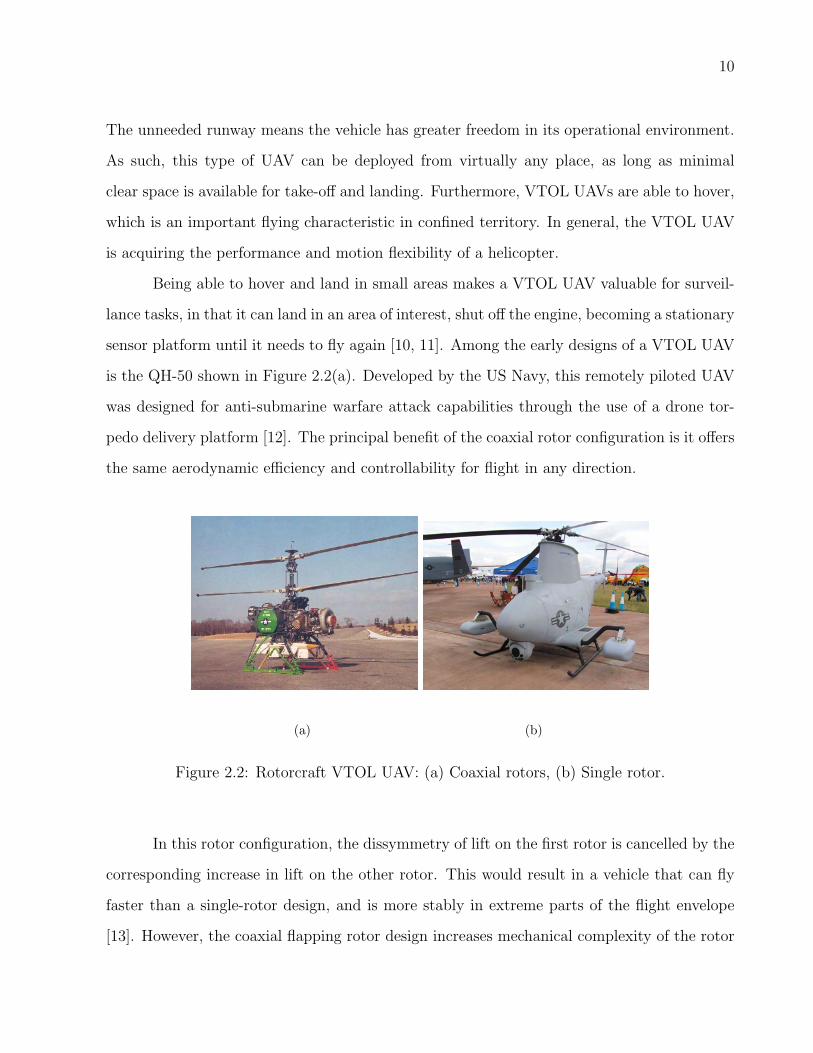
sensor platform until it needs to fly again [10, 11]. Among the early designs of a VTOL UAV

is the QH-50 shown in Figure 2.2(a). Developed by the US Navy, this remotely piloted UAV

was designed for anti-submarine warfare attack capabilities through the use of a drone tor-

pedo delivery platform [12]. The principal benefit of the coaxial rotor configuration is it offers

the same aerodynamic efficiency and controllability for flight in any direction.

(a) (b)

Figure 2.2: Rotorcraft VTOL UAV: (a) Coaxial rotors, (b) Single rotor.

In this rotor configuration, the dissymmetry of lift on the first rotor is cancelled by the

corresponding increase in lift on the other rotor. This would result in a vehicle that can fly

faster than a single-rotor design, and is more stably in extreme parts of the flight envelope

[13]. However, the coaxial flapping rotor design increases mechanical complexity of the rotor

11

hub, and also gives weight penalty. The linkages and swashplates for two rotor discs need

to be assembled around the rotor shaft, which itself is more complex because of the need to

drive two rotor discs in opposite directions.

These disadvantages are also true for the single rotor unmanned helicopter such as

the UAV shown in Figure 2.2(b). The complexity in the mechanical linkages is even further

increased in the singe rotor UAV. This is because the blades have to be flapped in order

to solve the dissymmetry of lift on the rotating blades, and usually needs an extra tail fan

to cancel the torque developed by the main rotor. Adapting a helicopter configuration also

means that the UAV has to use a very complicated cyclic and collective rotor control. A

study by the US Marine Corps has concluded that single rotor unmanned helicopters are

more expensive, less reliable, and offered no advantage to manned helicopters [14].

2.3 DEMANDS FOR SMALL DUCTED-FAN UAVS

Other than the design complexity in existing helicopter-type UAVs, due to their size, these

vehicles become less effective to carry out small scale missions. For missions in small units

situational awareness, local security, ISR, and target acquisition, these tasks are well suited

for small UAVs. In combat scenarios, small UAVs provide an immediate tactical responsive-

ness to the commanding unit, the task that larger UAVs cannot do as they are larger and

have extensive logistic requirements. Small UAVs also eliminate time delay by providing the

commander with the real-time information of the battlefield immediate to his surroundings,

over the hill, or behind the next building. These small vehicles can be deployed at the front

line of the battlefield, acting as flying ”binoculars”.

In applications other than military, small VTOL UAVs can be used for various law

enforcement operations, whether in urban environments or in remote areas. This UAV system,

with its onboard sensors, can assist in collecting evidence, performing long term surveillance,

and assessing hazardous situations prior to engaging any personnel. Because of its small

size, this UAV can be transported in back packs, or by standard ground vehicles to required

12

places. Although there is no unanimous standard to what constitutes a small UAV, the

following definitions are appropriate [7]:

• UAVs that are designed to be deployed independently: any UAV system where all

system components (air vehicle, ground control, interface, communication equipments)

are fully transportable by foot-mobile troops.

• UAVs that are designed to be deployed from larger aircraft: any UAV system where the

air vehicle can be loaded onto the larger aircraft without the use of mechanical loaders.

Several options are available in selecting the right VTOL UAV configuration for the

right job. Some of the configurations that have been adopted are a miniature version of a

normal helicopter [15, 16, 17], quadrotor [18], tilt-body , tilt-rotor [19], and fixed-wing tail-

sitter [20, 21]. Using a miniature helicopter model or quadrotor as a VTOL UAV platform

is very convenient since many of these models are readily available off-the-shelf. Usually the

designers need to do some modifications on the airframe, and add the controller hardware as

necessary to suit their applications. However, a significant weakness in helicopter-like vehicles

is they suffer from low speed forward flight [22], in addition to the configuration disadvantages

that we have discussed above.

Tilt-rotor UAV overcomes the low speed performance by converting to high speed

airplane mode once the take-off is completed. A major drawback in this configuration is the

need for the rotor and wing to tilt, adding to the design complexity of mechanical linkages and

control. The tail-sitter has the same ability to reach high speed flight, but this is achieved

by rotating the whole body horizontally. The tail sitter concept gives a very promising

solution for VTOL UAV configurations. It captures both VTOL and fixed-wing capabilities.

Nevertheless, the bare propeller of this configuration is prone to endangering the operator

and creates noise.

A small VTOL UAV configuration that has gained substantial interest in recent years

is the ducted-fan UAV. Some of articles that discuss ducted-fan UAVs can be found in [3,

13

23, 24, 25, 26]. A ducted-fan is a VTOL UAV that uses one or two fans (propellers) for

propulsion, and this fan is shrouded by a duct, also known as an annular wing. The forward

motion can be initiated by tilting the vehicle into the direction of motion. Usually, control is

achieved through flaps located inside the shrouded fan. Fan ducting is done for the following

reasons:

• Higher static thrust : when compared to a bare fan of the same diameter and power

loading, a ducted fan produces a higher static thrust. A higher static thrust means

the vehicle performance is better, especially during take-off. A detailed treatment of

deriving the static thrust from the duct is given in Section 3.4.2.

• Produces lift : since the duct itself is a revolved airfoil, by having a proper airfoil shape,

a large lift contribution can be generated with it. This gives extra lift, in addition to

the lift that is normally being produced by the wing.

• Low noise: by enclosing the fan, substantial noise level from a spinning fan or rotor can

be suppressed. This makes the vehicle a good candidate for covert missions.

• Safety : by enclosing the high spinning fan, it provides safety to the user, as well as the

vehicle. The vehicle becomes less fragile.

In the search for a suitable UAV to execute close range surveillance missions, the ducted-fan

UAV is found to be more advantageous than other VTOL vehicles, mainly because this UAV

can be designed in a very small size, compact, and portable. These features are usually crucial

for executing the mission effectively. In what follows, we will discuss several configurations of

existing ducted-fan UAVs, their variations, possible missions, and some difficulties faced by

them.

2.4 DUCTED-FAN VTOL UAV CONFIGURATIONS

In the past two decades, a number of development programs devoted to investigate the po-

tential of ducted-fan UAVs for various close range surveillance missions have been conducted.

14

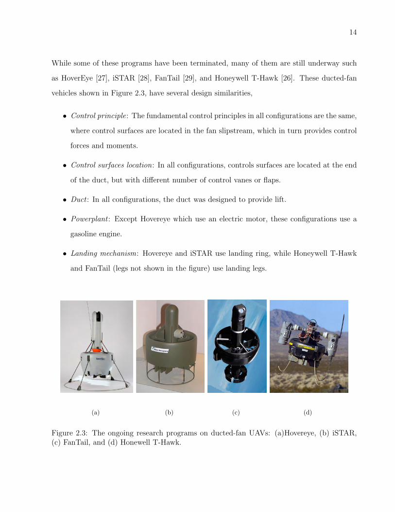
While some of these programs have been terminated, many of them are still underway such

as HoverEye [27], iSTAR [28], FanTail [29], and Honeywell T-Hawk [26]. These ducted-fan

vehicles shown in Figure 2.3, have several design similarities,

• Control principle: The fundamental control principles in all configurations are the same,

where control surfaces are located in the fan slipstream, which in turn provides control

forces and moments.

• Control surfaces location: In all configurations, controls surfaces are located at the end

of the duct, but with different number of control vanes or flaps.

• Duct : In all configurations, the duct was designed to provide lift.

• Powerplant : Except Hovereye which use an electric motor, these configurations use a

gasoline engine.

• Landing mechanism: Hovereye and iSTAR use landing ring, while Honeywell T-Hawk

and FanTail (legs not shown in the figure) use landing legs.

(a) (b) (c) (d)

Figure 2.3: The ongoing research programs on ducted-fan UAVs: (a)Hovereye, (b) iSTAR,(c) FanTail, and (d) Honewell T-Hawk.

15

Hovereye was developed as a VTOL UAV technology demonstrator to military specifi-

cations for very short range combat intelligence [27]. The compact design of Hovereye makes

it very portable, and it is designed to operate in complex, confined, and congested environ-

ments. This vehicle is 70 cm in height, 50 cm diameter, and 4 kg weight with 300 g payload.

Powered by an electric motor, the endurance of Hovereye can last up to 10 min, and has

the nominal range of 1500 m. Since Hovereye is powered by an electric motor, it is a low

noise flying platform. Hovereye can reach a maximum speed of 48 km/h in the presence of

32 km/h wind speed.

Another similar ducted-fan UAV configuration is iSTAR (intelligence, surveillance,

target acquisition and reconnaissance), developed by Allied Aerospace in a number of sizes

ranging from 9” to 29” duct diameters. The main project goal was to develop a UAV that can

be launched, recovered, and refueled from a mobile platform in order to provide defense force

extension through autonomous aerial response [10]. It has undergone several flight tests and

demonstration programs including high speed flight where the vehicle was tilted at an extreme

pitch angle. A discussion on the automated launch, recovery, and refueling of this vehicle can

be found in [30], and the estimation of vehicle aerodynamic can be found in [31, 32].

ST Aerospace has also developed a ducted-fan UAV, called Fantail to perform various

surveillance tasks. It has the ability to achieve a high speed forward flight at almost horizontal

orientation. It has two variants of 3 kg and 6.5 kg, which makes this vehicle more versatile

to meet various surveillance applications. Probably the best progress made until now was

from the Honeywell T-Hawk program, as this vehicle was deployed in a real conflict zone in

2007, and was also reported to have received overseas orders [33]. This UAV, shown in Figure

2.3(d) has a loaded weight of 8.4 kg, and uses two small gasoline engines for propulsion. The

Honeywell T-Hawk has an endurance of 40 minutes, rate of climb of 7.6 m/s, and a maximum

forward flight speed of 90 km/h in the presence of 37 km/h winds. A thorough discussion on

the aerodynamic of this vehicle can be found in [26, 34].

16

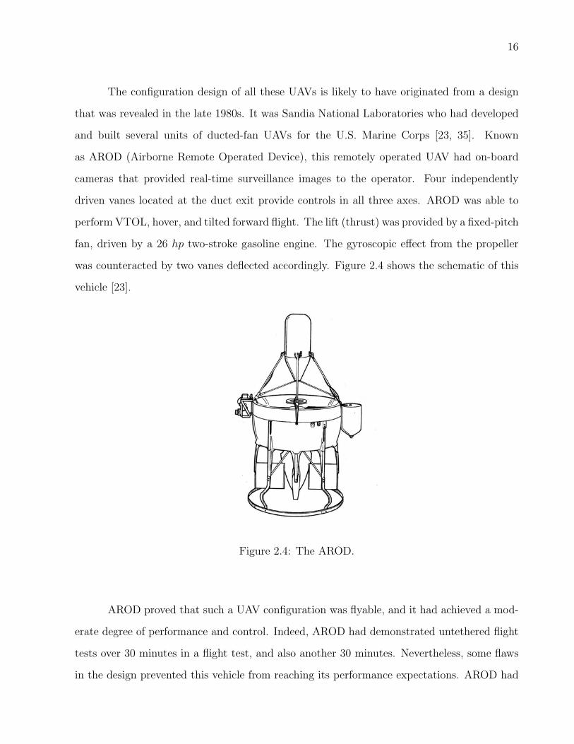
The configuration design of all these UAVs is likely to have originated from a design

that was revealed in the late 1980s. It was Sandia National Laboratories who had developed

and built several units of ducted-fan UAVs for the U.S. Marine Corps [23, 35]. Known

as AROD (Airborne Remote Operated Device), this remotely operated UAV had on-board

cameras that provided real-time surveillance images to the operator. Four independently

driven vanes located at the duct exit provide controls in all three axes. AROD was able to

perform VTOL, hover, and tilted forward flight. The lift (thrust) was provided by a fixed-pitch

fan, driven by a 26 hp two-stroke gasoline engine. The gyroscopic effect from the propeller

was counteracted by two vanes deflected accordingly. Figure 2.4 shows the schematic of this

vehicle [23].

Figure 2.4: The AROD.

AROD proved that such a UAV configuration was flyable, and it had achieved a mod-

erate degree of performance and control. Indeed, AROD had demonstrated untethered flight

tests over 30 minutes in a flight test, and also another 30 minutes. Nevertheless, some flaws

in the design prevented this vehicle from reaching its performance expectations. AROD had

17

only attained a steady speed of 28 km/h in a 20o tilt angle forward flight with zero rate of

climb. At this magnitude of tilt angle, the measured forward speed was considered too slow

from the targeted speed of 56 km/h. AROD also encountered stability problems during the

flight, and this prevented it from realizing its full capabilities [36]. In addition to this stabil-

ity problem, AROD was too bulky (36 kg MTOW) to be assigned to close range surveillance

tasks.

In all ducted-fan UAV configurations discussed above, including AROD, the forward

speed attained was between 28 km/h to 90 km/h. This limited forward speed can prevent

these vehicles from performing some tasks effectively. In a combat scenario, the situation

is chaotic, unpredictable, and life-threatening. We are moving into an era where response

time and information are the best defense. Commanders with the most accurate, real-time

knowledge of the battlefield will have an advantage over their opponents. This can be attained

with the help of fast, efficient, and accurate supportive units including platoons and UAVs.

In addition to having VTOL capabilities, acquiring a fleet of small ducted-fan UAVs that can

fly with a higher forward speed is an overwhelming advantage. We will address this issue in

more detail in Section 3.1.

2.5 CHALLENGES AND APPROACHES TO AUTONOMOUS CONTROL

OF DUCTED-FAN UAVS

The complex aerodynamic of the ducted-fan in vertical flight is associated with flying at a

high angle of attack (α). At hover, the airflow into the duct is symmetric, hence the lift

generated around the duct is balanced. This is indicated in Figure 2.5(a) where the lift

produced at one side of the duct lip, LW (windward) is equal to the other side, LL (leeward).

However, there is a problem when the duct (vehicle) is tilted, and consequently moving to

the tilted direction. This motion is denoted as Low-speed Tilted Flight (LSTF), shown in

Figure 2.5(b). Since the airflow into the duct is not symmetrical anymore, the asymmetric

flow causes a higher α on the windward side of the duct than on the other side.

18

LW

(a) Hover: V=0, Fx=0, M=0

L

W

α

(b) LSTF: V, F, M > 0

Figure 2.5: Duct aerodynamic at hover and forward flight.

As a higher α is generated at the windward side, more lift is produced here than at

leeward side. This imbalanced lift causes a large positive pitching moment (M), which tends

to turn the thrust axis away from the direction of motion. This situation repeats at the other

side, resulting in an even bigger moment. This demonstrates that the vehicle is dynamically

unstable. The tilted orientation in LSTF is also encounters a drag force, D. The vehicle also

encounters a similar problem when hovering in wind gust. Here, the existence of the drag

requires the vehicle to tilt into the wind gust in order to maintain a steady hover.

However, the gust generated corrective moment resists the tendency for the vehicle

to tip into the wind [26]. Another problematic issue is that the aerodynamic moments are

very sensitive to changes in flight conditions, their dependence on relative wind is nonlinear

and complex to be modeled. This scenario causes the operation of the ducted vehicle to be

very difficult, and thus requires the aid of a sophisticated controller [37]. Furthermore, the

inherent instability of the ducted-fan UAV has hindered it from flying without the assistance

of artificial stabilization system [27], and in fact this instability and nonlinear nature of a

small ducted-fan UAV that hovers and transitions to forward flight make the control system

19

design a very challenging one. The ability to perform transition maneuvers from and to

vertical flight as part of the design requirement is the greatest challenge in the development

of the controller. In what follows, we discuss several control techniques applied to ducted-fan

UAVs.

2.5.1 Conventional Flight Control System

White [35] considered a conventional linear quadratic regulator (LQR) synthesis to stabilize

a ducted-fan UAV. The UAV was flown by tele-operation, and the LQR design methodology

was used to provide stability augmentation through control axes decoupling. The vehicle was

represented by a linear dynamics model, and three LQR control loops were used. A full state

feedback was required to ensure LQR robustness. Indeed, under some reasonable assumptions

it was possible to guarantee the stability of the closed loop system. Two single-input single-

output (SISO) LQR loops were used for roll rate and altitude rate control respectively, while

one multiple-input multiple-output (MIMO) loop was used for pitch and yaw controls. It

is important to note that this approach may be reliable for a vehicle where linearity in the

system is dominant.

An automatic stabilization using backstepping techniques was discussed in [24]. It

describes a control strategy to automatically stabilize the hovering position of the ducted-fan

UAV in the presence of wind gusts. The method has allowed the gyroscopic coupling to

diminish, by taking advantage of the thrust mechanism, and through yaw rate decoupling

from the rest of the system dynamics. Decoupling dynamics are much easier to handle

in analytical studies, allowing a much more convenient way to access the control system

performance, at the expense of losing some accuracy in representing the vehicle dynamics.

Another important point is the backstepping technique estimates the aerodynamic forces and

moments concurrently, while stabilizing the vehicle. This is a great feature in the proposed

method since the disturbance gust is hard to measure accurately, therefore such estimation

technique would be beneficial, if done properly.

20

Another linear approach in ducted-fan UAV control was carried out by Lipera et al.

[28]. Here, the classical PID control was used to design the flight controller for a small vari-

ant of the iSTAR UAV. The vehicle model used was a linearized state-space model, with

aerodynamic derivatives obtained though wind tunnel experiments. The analysis involved

pilot-in-the-loop simulation and also flight tests. Avanzini et al. [38] has used a SISO con-

troller for the outer loop autopilot, while robust stability and uncoupled response of the

ducted-fan UAV was realized by a MIMO controller in the inner loop. Because of the con-

sidered ducted-fan vehicle considered in this study involves nonlinearities, for example the

presence of nonlinear couplings in hovering in crosswinds, it makes the linear control approach

inefficient.

Johnson [3] used an autonomous adaptive controller to correct the modeling errors

present in a simple linear model of the vehicle. The adaptive control approach was found

to be well suited especially at near hover conditions, with flight test performance success-

fully predicted by the simulation result. Also, the controller was able to closely follow the

commanded trajectory in vertical flights with just a little overshoot. However, the controller

had difficulty in tracking the commanded signals for transition maneuvers. This was due to

limitations in the used adaptive element.

A more appropriate approach to control the envelope of ducted-fan UAV flights is

through nonlinear modeling. In working with a similar small ducted-fan UAV, Christina et

al. [39] presented a nonlinear controller for a small ducted-fan UAV based on the dynamics

inversion technique. The technique is a control law design methodology that cancels out

the vehicle dynamics so that the vehicle acceleration matches the command to the dynamics

inversion. It requires full knowledge of the physical model, where full state feedback is needed,

together with the data of the vehicle obtained from wind tunnel experiments. The main

advantage of the full nonlinear dynamics inversion method is it obviates the needs for gain

scheduling regulators in each flight condition. Also, the cross couplings between controls are

eliminated.

21

A theoretical framework of nonlinear robust control on a ducted-fan MAV (Micro Air

Vehicle) is discussed in [40]. Here, the authors considered trajectory control problems in

all vertical, longitudinal, and lateral flights. A nonlinear robust regulator was designed to

track the reference performance asymptotically, subject to some restrictions in higher order

reference time derivatives. The problem of tracking a reference signal was formulated as a

state constrained tracking problem for a chain of integrators. The robustness of the controller

was measured by observing if vehicle states satisfy the prepositions of control laws placed in

the asymptotic bound. As a whole, the objective of the robust control system was to ensure

the ducted-fan UAV did not overturn and the longitudinal-lateral dynamics asymptotically

approached the desired references.

In general, most of control methods applied to ducted-fan UAVs are based on the

conventional flight control system structure. It was based on SISO structure, designed to

control the vehicle at an instantaneous airspeed and altitude. Nonlinearities were handled

through gain scheduling that covered multiple flight regimes. The problem associated with

this approach is the coupling between the separate controllers, which can result in a long

trial-and-error design process [41]. The nonlinear control approach in [39] is quite promising,

and has proven to be very successful, however an accurate model of the vehicle is required,

which is something not readily available and difficult to obtain at an early design stage. The

proposed robust controller in [40], though has highlighted several conditions needed for vehicle

robustness. However, it is very theoretical and has yet to be proven to be a practical method

at the early stage of the design process.

2.5.2 Intelligent Flight Control System

Intelligent systems can be built from various approaches ranging from conventional control

such as optimal control, robust control, stochastic control, linear control, and nonlinear con-

trol, as well as the more recent soft computing techniques: fuzzy logic, genetic algorithm, and

neural network. Regardless of the intelligent methods used, there are several attributes that

22

an intelligent system should have, including [42]:

• Learning: capability to acquire new behaviors based on past experience.

• Adaptability: capability to adjust responses to a changing environment or internal

conditions.

• Robustness: consistency and effectiveness of responses across a broad set of circum-

stances.

• Information compression: capability to turn data into information and then into ac-

tionable knowledge.

• Extrapolation: capability to act reasonably when encountering a set of new (not previ-

ously experienced) circumstances.

The aim to build an intelligent system is mostly to ensure safe and reliable performance of

complex systems with minimal or no human intervention. Specifically, the role of an intelligent

system in aerospace engineering is twofold [43]:

• To function as an intelligent assistant to augment human expertise.

• To substitute human expertise, in the effort to save cost, time, and life.

The second role of an intelligent system in aerospace applications is very well suited to our

application, which is to substitute human pilots with an autonomous intelligent flight control

system. For a ducted-fan UAV, the complexity of the problem makes the intelligent approach

very beneficial. Among the difficulties associated with the design of a flight control system

is the complexity in the vehicle dynamics. The variables are highly coupled and it is very

difficult to decouple the system adequately to implement conventional control methods. The

choice of an intelligent technique depends heavily on the design requirement.

Since our purpose is to substitute a human pilot in controlling the UAV, it deduces that

the best technique to implement is a system than can imitate how humans think and respond.

23

Interestingly, this is precisely one of the attributes associated with fuzzy logic. Fuzzy logic

is an artificial intelligence technique that is able to reason, and solve problems that normally

requires human intelligence [44]. When referring to the intelligent attributes listed above,

fuzzy logic has the attributes of adaptability, robustness, and information compression.

The presence of uncertainties and nonlinearities in both the aerodynamic and dynamics

models of the ducted-fan UAV causes difficulties in understanding the complete behaviour

of the vehicle. As a result, controlling the vehicle is even more challenging. However, fuzzy

logic has an additional advantage which is the ability to explore an effective tradeoff between

precision and cost in developing an approximate model of a complex system. Fuzzy logic

has also proven to be robust enough in the presence of uncertainties and disturbances in the

system [45, 46].

Besides, it is an established fact that fuzzy logic is a universal approximator for non-

linear control systems, and general enough to provide the desired nonlinear control actions

through careful adjustment [47, 48]. It is an alternative to the conventional approaches since

this soft computing technique is able to construct a nonlinear controller using heuristic infor-

mation [49]. It allows the design of knowledge-based controllers without requiring a precise

model and also provides a highly flexible and adjustable mechanism that is useful when an

accelerated development is required [50].

As a generic rule, a good control system design practice is that it must be able to

efficiently use all of the information available. There are two sources of control information:

sensors, that provide numerical measures of system variables, and human experts, who provide

linguistic descriptions about the system behaviour and best control practices. Fuzzy logic is

a control tool that can handle both kinds of information sources, thus it can be applied

when there is a lack in one of them [51]. Fuzzy logic is also a model-independent approach.

The model-independent approach makes the control system design easier, since obtaining an

accurate mathematical model of the ducted-fan UAV is difficult.

24

Due to the reasons stated above, fuzzy logic has made its way into a vast number of

aerospace applications, including unmanned vehicles. The fuzzy logic scheme has also been

applied to the autopilot system design [52, 53]. Control of aggressive manoeuvers of unstable

aircraft using fuzzy logic can be found in [54]. Other applications of fuzzy logic in various

aerospace fields can be found in [55, 47, 56, 57, 58]. In UAV applications, fuzzy logic has

been used as an autonomous controller [59, 60, 50].

A specific application of fuzzy logic to ducted-fan UAV control was done by Wonseok

and Bang [61]. The issues described in this paper is quite common to ducted-fan UAV, where

the vehicle is unstable and susceptible to wind due to its external shape. The vehicle must also

change the attitude to gain speed (tilted to the flight path), so it has different characteristics

with respect to velocity. Here the author has used fuzzy gain scheduler control (GSC) to

solve this problem. Generally, the use of GSC is to control nonlinear systems by switching

between a series of linear controllers. These linear controllers are selected according to the

system operating point where at one particular time, the controller’s gain has to be set. For

the problem discussed in [61], fuzzy logic has been used to ‘schedule’ the appropriate gain at

different flight attitudes.

Unlike in fuzzy logic control, in order to apply gain scheduling control, we have to

linearize the controller at several desired operating points. At one particular point the linear

model is an approximation of the nonlinear model and the controller performance should be

within design parameters. However, as the system moves from that point, the linear model

becomes a less accurate representation and control performance will deteriorate [62]. For

many systems with nonlinearities, this situation makes the design of a single controller that

gives adequate performance across the operating range is difficult.

One of the solutions to this problem is to use a fully fuzzy logic controller. It means the

whole controller itself was developed by using fuzzy logic. The controller is solely depends on

the fuzzy logic architecture, and no other controllers are embedded in the system. The reason

for depending only on fuzzy logic is as discussed above. In what follows, we will develop some

25

fundamental aspects of fuzzy logic.

2.6 FUZZY LOGIC THEORY

Fuzzy logic is a set of mathematical principles for knowledge representation based on the

degree of membership, rather than on the crisp membership of classical binary logic [63].

In contrast with binary Boolean logic, fuzzy logic is multi-valued and deals with degrees of

membership and degrees of truth. Boolean logic uses crisp values of 0 (false) or 1 (true),

while fuzzy logic uses the continuum of logical values between 0 and 1, as shown in Figure

2.6. Instead of just black and white, fuzzy logic employs a spectrum of colors, accepting that

things can be partly true and partly false at the same time [64, 65, 66].

(a) (b)

Figure 2.6: Range of logical values: (a) Boolean logic, (b) Multi-value logic.

Fuzzy logic reflects and models how people think. In everyday language we usually say

words in forms that are less precise. For example, we would normally say ‘the box is heavy ’,

‘the weather is pretty hot ’, or ‘this room is small ’. The terms heavy, hot, and small are clearly

understood, but cannot be expressed in an equation because these terms are not quantities,

as which weight, temperature, and volume are. Here fuzzy logic is available to model such

vague and ambiguous terms. Fuzzy logic attempts to model our sense of words, our decision

making and our common sense. It serves as a bridge between mathematics and language. As

a result, it leads to new, more human, and intelligent systems .

The theory of fuzzy sets and fuzzy logic is well founded and understood. It has existed

for over 40 years since Lotfi Zadeh [63] rediscovered fuzziness, identified it, and explored it in

26

1965. Fuzzy set theory has shown to be extremely useful in many control applications as well

as non-control applications requiring decision making in uncertain environments [50]. In the

context of control applications, it excels in systems which are very complex, highly nonlinear,

and have parameter uncertainties [67]. It has been used in a number of problem domains

include chemical engineering, manufacturing, mineral engineering, and aerospace engineering

[68]. One of the reasons for the success of fuzzy logic is that the linguistic variables, values, and

rules defined in it allow the engineer to seamlessly translate human knowledge into systems

that work [69].

2.6.1 Fuzzy Sets

Fuzzy logic is based on fuzzy sets. Let us begin with a quick review of classical set theory. The

range of possible quantitative values considered for fuzzy set members is called the universe

of discourse. Suppose X is the universe of discourse and let its elements is denoted as x.

For a classical set theory, crisp set A of X is defined as fA(X), known as the characteristic

function of A:

fA(x) : X → 0, 1, (2.1)

where,

fA(x) =

1, if x ∈ A

0, if x /∈ A

This set maps universe of discourse X to a set of two elements. For any elements x of

universe of discourse X, the characteristic function fA(x) is equal to 1 if x is an element of

set A, and is equal to 0 if x is not an element of A. These classical sets are also referred to as

crisp sets. That is, classical set theory imposes a sharp boundary on this set and gives each

member of the set the value of 1, and all members that are not within the set the value of 0.

In other words, for a classical set, an object is either in a set or it is not, as can be seen in

Figure 2.7(a).

27

An element

not in A

An element in A

Sharp

boundary An element that

has a degree of

membership

between [0,1] in

set A

Fuzzy

boundary

X universe X universe

Set A Set A

(a) (b)

Figure 2.7: Theory of sets: (a) Classical set, (b) Fuzzy set.

A new type of set theory, known as fuzzy set theory was introduced by Lotfi Zadeh [63]

that allows the representation of concepts that previously are not well defined [70]. Unlike

the classical set, we have a different description of a fuzzy set that is capable of providing

a graceful transition across a boundary. In other words, we can describe a fuzzy set as a

mathematical set with fuzzy boundaries, or a set without a crisp, a clearly defined boundary.

The representation of a fuzzy set is depicted in Figure 2.7(b). A fuzzy set A of universe of

discourse X is defined by the function µA(x).

µA(x) : X → [0, 1] (2.2)

where,

µA(x) = 1, if x is totally in A

µA(x) = 0, if x is not in A

0 < µA(x) < 1, if x is partly in A

This fuzzy set allows a continuum of possible choices. For any element x of universe

of discourse X, the membership function µA(x) equals the degree to which x is an element of

set A. This degree, which is a value between 0 and 1, represents the degree of membership

of element x in set A. As can be seen in Equation (2.2), an object or element can belong to

28

a set with a continuum grade of membership ranging between zero and one. It also indicates

the membership function µA(x) can be partially true in the set A. Now assume the universe

of discourse X is a crisp set contains five elements X = x1, x2, x3, x4, x5. Let A be a crisp

subset of X and assume that A consists of only two elements, A = x2, x3. Subset A can

now be described by:

A = (x1, 0), (x2, 1), (x3, 1), (x4, 0), (x5, 0)

which is in the form of pairs xi, µA(xi), where µA(xi) is the membership function of element

xi in the subset A. Here we notice the membership functions are either 0 or 1. This indicates

a special case where a crisp set can also become a subset of the fuzzy set, and this is shown

in Figure 2.8. We can generalize if set A is a subset of X, then A is said to be a fuzzy subset

of X if and only if,

A = x, µA(x), x ∈ X,µA(x) : X → [0, 1] (2.3)

X Universe)(xµ

x

1

0

Fuzziness FuzzinessCrisp subset A

Fuzzysubset A

Figure 2.8: Representation of crisp and fuzzy subset of X

and is a fuzzy set A, that is also a fuzzy subset of X which can be expressed as,

A = x1, µA(x1), x2, µA(x2), ..., xn, µA(xn) (2.4)

29

In order to represent a continuous fuzzy set, we need to express it as a continuous

function and then map the elements of the set to their degree of membership accordingly.

The functions which are known as membership functions are available in various types, and

will be discussed in the following section.

2.6.2 Membership Functions and Logical Operators

A membership function (MF) is a function that defines how each point in the universe of

discourse (input space) is mapped to a membership value (degree of membership) between 0

and 1 [71]. As can be seen in Figure 2.8, the fuzziness in a fuzzy set is characterized by its

membership functions. The degree of membership function of an element x (x ∈ X) in the

universe of discourse X is denoted by µA(x). The function itself can be an arbitrary curve,

which its shape can be defined as a function that suits the designer from the point of view of

simplicity, convenience, speed, and efficiency. A membership function is also chosen on the

basis of how well it will describe the set that it represents.

The typical functions are built from several basic functions such as piecewise linear

functions, the Gaussian distribution function, the sigmoid curve, quadratic, and cubic polyno-

mial curves. Most applications use linear functions primarily because of their simplicity and

lower computation time requirements [72, 73]. From these linear functions which are formed

using straight lines, the triangular and trapezoidal membership functions are widely chosen.

These types of membership functions, with some other types, are shown diagrammatically in

Figure 2.9.

The term logic associated with fuzzy logic indicates the involvement of some logical

operations in it. Fuzzy logic is a superset of Boolean logic in which at its extreme fuzzy values

of 1 (completely true) and 0 (completely false), the standard logical operations of AND, OR,

and NOT will take place. The standard truth tables of logical operations are shown in Table

2.1. Now, as we have already discussed, not only logical crisp values of 0 and 1 are accepted

in fuzzy logic, rather it is a matter of degree between 0 and 1 that represents the truth of any

30

0 2 4 6 8 10

0

0.25

0.5

0.75

11

Universe of discourse, X

Deg

ree

of m

embe

rshi

p

Triangular

0 2 4 6 8 10

0

0.25

0.5

0.75

1 1

Universe of discourse, X

Deg

ree

of m

embe

rshi

p

Trapezoidal

0 2 4 6 8 10

0

0.25

0.5

0.75

11

Universe of discourse, X

Deg

ree

of m

embe

rshi

p

Gaussian

0 2 4 6 8 10

0

0.25

0.5

0.75

11

Universe of discourse, X

Deg

ree

of m

embe

rshi

p

Bell-shaped

0 2 4 6 8 10

0

0.25

0.5

0.75

11

Universe of discourse, X

Deg

ree

of m

embe

rshi

p

Sigmoidal

0 2 4 6 8 10

0

0.25

0.5

0.75

11

Universe of discourse, X

Deg

ree

of m

embe

rshi

p

Z-shaped

0 2 4 6 8 10

0

0.25

0.5

0.75

11

Universe of discourse, X

Deg

ree

of m

embe

rshi

p

S-shaped

0 2 4 6 8 10

0

0.25

0.5

0.75

11

Universe of discourse, X

Deg

ree

of m

embe

rshi

p

pi-shaped

Figure 2.9: Membership function types.

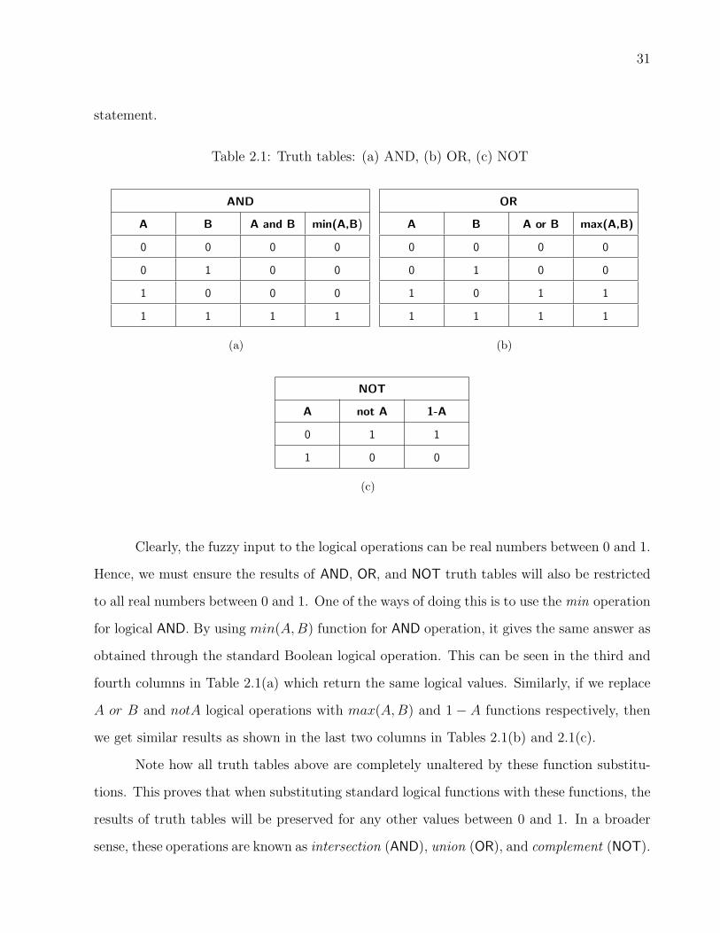
31

statement.

Table 2.1: Truth tables: (a) AND, (b) OR, (c) NOT

AND

A B A and B min(A,B)

0 0 0 0

0 1 0 0

1 0 0 0

1 1 1 1

(a)

OR

A B A or B max(A,B)

0 0 0 0

0 1 0 0

1 0 1 1

1 1 1 1

(b)

NOT

A not A 1-A

0 1 1

1 0 0

(c)

Clearly, the fuzzy input to the logical operations can be real numbers between 0 and 1.

Hence, we must ensure the results of AND, OR, and NOT truth tables will also be restricted

to all real numbers between 0 and 1. One of the ways of doing this is to use the min operation

for logical AND. By using min(A,B) function for AND operation, it gives the same answer as

obtained through the standard Boolean logical operation. This can be seen in the third and

fourth columns in Table 2.1(a) which return the same logical values. Similarly, if we replace

A or B and notA logical operations with max(A,B) and 1 − A functions respectively, then

we get similar results as shown in the last two columns in Tables 2.1(b) and 2.1(c).

Note how all truth tables above are completely unaltered by these function substitu-

tions. This proves that when substituting standard logical functions with these functions, the

results of truth tables will be preserved for any other values between 0 and 1. In a broader

sense, these operations are known as intersection (AND), union (OR), and complement (NOT).

32

The intersection and union of two fuzzy sets A and B on the universe of discourse X are

specified by Equation 2.5 and 2.6 respectively, which aggregate two membership functions

µA(x) and µB(x). As for complement, it is obtained through Equation 2.7, where x ∈ X.

µA∩B(x) = min[µA(x), µB(x)] = µA(x) ∩ µB(x) (intersection) (2.5)

µA∪B(x) = max[µA(x), µB(x)] = µA(x) ∪ µB(x) (union) (2.6)

µ¬A(x) = 1− µA(x) (complement) (2.7)

2.6.3 Linguistic Variable and Hedges

Linguistic variable is whose value are words rather than numbers [71]. The concept of lin-

guistic variable is the root of the fuzzy set theory. A linguistic variable is also known as

fuzzy variable. For instance, the statement ’weather is hot ’ implies that the linguistic vari-

able weather takes the linguistic value hot. Although words are inherently less precise than

numbers, their usage is closer to human intuition as depicted in Figure 2.10.

(a) (b)

Figure 2.10: Solving a real world problem: (a) Precision, (b) Significance.

In fuzzy logic, linguistic variables are used in fuzzy rules such as,

33

IF wind is strong, THEN throttle is big

IF fuel is low, THEN mission is short

where in these examples the linguistic variables are wind and fuel, whereas their linguistic

values are strong and low. The fuzzy rules will be discussed in a greater detail in the next

section. Attached to a linguistic variable is fuzzy qualifier, called hedges. Hedges are terms

that modify the shape of fuzzy sets. They may include adverbs like very, somewhat, quite,

more or less, and slightly. Hedges can possibly modify verbs, adjectives, adverbs or even the

whole sentences and they are used as:

• All purpose modifiers such as very, quite, or extremely.

• Truth values, such as quite true or mostly false.

• Probabilities, such as likely or not very likely.

• Quantifiers, such as most, several, or few.

• Possibilities, such as almost impossible or quite possible.

Hedges perform concentration and dilation to fuzzy sets. For example, in the set of

high thrust, hedge very performs concentration and it derives the subset of very high thrust.

Another hedge such as extremely serves the same purpose to a greater extent. The operation

of dilation expands the set. Such hedge like more or less expands the set. The set of more or

less high thrust is broader than the set of high thrust. Hedges also break down continuums

into fuzzy intervals. To describe the linguistic variable thrust, we can use hedges like very

low, moderately low, slightly low, neutral, slightly high, moderately high, and very high.

The principal structure of a fuzzy logic system is shown in Figure 2.11. There are four

basic components: fuzzification, rule base, fuzzy inference, and defuzzification. In the next

two sections, we develop some fundamentals of these components.

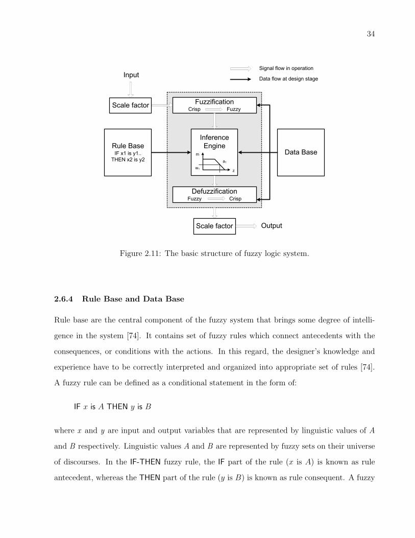
34

FuzzificationCrisp Fuzzy

Inference

Engine

DefuzzificationFuzzy Crisp

Input

Output

Rule BaseIF x1 is y1..

THEN x2 is y2

Data Base

Signal flow in operation

Data flow at design stage

m

z

a1

w1

Scale factor

Scale factor

Figure 2.11: The basic structure of fuzzy logic system.

2.6.4 Rule Base and Data Base

Rule base are the central component of the fuzzy system that brings some degree of intelli-

gence in the system [74]. It contains set of fuzzy rules which connect antecedents with the

consequences, or conditions with the actions. In this regard, the designer’s knowledge and

experience have to be correctly interpreted and organized into appropriate set of rules [74].

A fuzzy rule can be defined as a conditional statement in the form of:

IF x is A THEN y is B

where x and y are input and output variables that are represented by linguistic values of A

and B respectively. Linguistic values A and B are represented by fuzzy sets on their universe

of discourses. In the IF-THEN fuzzy rule, the IF part of the rule (x is A) is known as rule

antecedent, whereas the THEN part of the rule (y is B) is known as rule consequent. A fuzzy

35

rule can also have multiple antecedents and consequents, which results from a multi-inputs

multi-outputs fuzzy system such as:

IF wind is weak, AND weight is light, AND target altitude is low

THEN throttle is low, elevator is neutral

In this case, all rule antecedents are calculated simultaneously and resolved in a sin-

gle number, using fuzzy set operations discussed in the previous section. The ideal case in

developing fuzzy system, is that the rule base should comprise all possible IF-THEN combi-

nation of linguistic values among input variables. Consider the above example which is a

3-inputs 2-outputs fuzzy system. The input variables for this fuzzy system are wind, weight,

and target altitude, while the output variables are throttle and elevator.

Although IF-THEN rules have been used widely in expert systems, their use is only

for crisp value which is either completely true or completely false. Whereas in fuzzy logic

system, if the rule antecedent is true, the rule consequent is true to some extent, or in other

words they are partially true. The central idea is, if the rule antecedent is true to some

degree of membership, then the rule consequent is also true to that same degree. This is the

fundamental characteristic of fuzzy logic rule that distinguishes it from the classical Boolean

logic.

In the 3-inputs 2-outputs fuzzy system above, suppose each input variable is repre-

sented by five hedges: extreme, very, moderate, slight, and little. Fuzzy rules are produced

by combining all linguistic values available in input variables. Therefore in this example, the

maximum number of rules that can be produced are 5 × 5 × 5 = 125. Observe that many

of the consequent needed for 125 possible antecedent combinations are readily apparent. For

instance, when the wind is very strong, weight is very heavy, and target altitude is very high,

then logically we will know that the throttle will be very high.

It seems that the generation of fuzzy rules is quite straightforward. However, as we

will see later, this is not the case for nonlinear systems where most of the governing equations

are coupled to each other. A more careful approach is needed to deal with such matter. In

36

selecting linguistic values to represent all input and output variables, there is not a definite

method available. However, in doing so, we have to ensure their definitions should reflect and

are consistent with the normal meaning of the terms [75].

Similar to the nature of selecting the linguistic values, the production of rule base

depends on the designer’s skill and knowledge in dealing with such systems. Generally, as

the number of fuzzy rules increase, the fuzzy system becomes more complicated, although

this does not guarantee that a more better solution is achieved. In the first stage of fuzzy

logic control design, the method of producing the rules is the old fashioned trial-and-error

approach directed by the experience in controlling the system [75].

While the rule base contains a number of fuzzy rules, the data base is the storage for

input and output membership functions data for each specific task. It contains various types

of data, depending on the system under consideration. In the UAV control, the database

includes the aerodynamic data of the vehicle, the dynamical relationship between control

surfaces and body, and the propulsive data. This is the place where the expert knowledge is

accumulated before being used in the system.

2.6.5 Fuzzification, Fuzzy Inference, and Deffuzzification

Fuzzification is the process of converting crisp input data to a degree of membership by a

lookup in one or several membership functions. That is, to convert the crisp input variable

into fuzzy variable. The reverse process is defuzzification, which converts the fuzzy output

into crisp output. The process that occurred between fuzzification and defuzzification is called

fuzzy inference. It is a process of formulating a mapping from a given input to an output,

and it has two distinct parts [76]. The first part is evaluating the rule antecedent, and the

second part is the implication or applying the result to the consequent . In classical Boolean

logic, if the rule antecedent is true, then the rule consequent is also true. However this is not

the case in fuzzy logic rule operation.

As we have discussed before, in fuzzy logic if the rule antecedent is true to some degree

37

of membership, then the rule consequent is also true to that same degree. To infer the fuzzy

system is to have a precise single number of the final output even in the preceding processes

it involved the use of fuzzy variables. We present an example that demonstrates all steps

involved in building a fuzzy logic controller (FLC). It is a 2-inputs 1-output FLC for UAV in

vertical flight that has three rules as shown in Table 2.2. While other variables are assumed

under control, basically in this example the FLC is assigned to control the throttle setting

based on the wind condition and target altitude. Here we used the Mamdani inference method,

named after its inventor Professor Ebrahim Mamdani who first introduced the technique in

1975 [77].

Table 2.2: Example of 2-inputs 1-output FLC for UAV in vertical flight.

Rule 1 Rule 1

IF a is A3 IF still air is good

OR b is B1 OR target altitude is low

THEN c is C1 THEN throttle open is small

Rule 2 Rule 2

IF a is A2 IF still air is average

AND b is B2 AND target altitude is high

THEN c is C2 THEN throttle open is medium

Rule 3 Rule 3

IF a is A1 IF still air is bad

THEN c is C3 THEN throttle open is big

In Table 2.2, the linguistic variables are still air, target altitude, and throttle open are

denoted as a, b, and c respectively. The linguistic values A1, A2, and A3 (bad, average,

38

and good) are determined by fuzzy sets on the universe of discourse A (still air). Linguistic

values B1 and B2 (low and high) are determined by fuzzy sets on the universe of discourse

B (target altitude). Finally, linguistic values C1, C2 and C3 (small, medium, and big) are

determined by fuzzy sets on the universe of discourse C (throttle open). The steps of building

a fuzzy logic controller are fuzzification, rule evaluation, aggregation of the rule outputs,

and defuzzification as follows, which the second and the third steps are defined as Mamdani

inference method.

• Step 1 : Fuzzification

The inputs of the FLC are still air (a1 ) and target altitude (b1 ) are shown on the top

side of Figure 2.12. First is to fuzzify these crisp inputs, that is to find out the degree

to which these inputs belong to each of the corresponding fuzzy sets. The crisp inputs

a1 and b1 are limited to their universe of discourse. The ranges of the universe of

discourses are determined from data base which is obtained through experimentation,

simulation, or experience. Consider the variable still air, which the value indicates the

current strength of wind. If the still air is bad, it simply means there is strong windy

conditions at site.

The typical magnitude of the wind, its minimum, average, and maximum are obviously

gathered through observation and measurement at site, or obtained through other avail-

able database. Therefore, this data gives us the information on the range of universe of

discourse A. As for the second input variable, b1, it is the variable set by the user. The

user usually sets the altitude that the UAV is required to reach, and its maximum limit.

The maximum reachable altitude is the maximum limit on the universe of discourse B,

which depends on the vehicle performance data.

Suppose at one particular time, when the percentage of still air is 35%, and the tar-

get altitude is set at 60%, we would like to know what the corresponding throttle open of

the UAV is. In short, the problem can be stated as: when inputs a1=35% and b1=60%,

what is the output c1?. All we have to do is to project a straight line from fuzzy set a1

39

Crisp inputa1

0 a1

OR(max)

AND(min)

Fuzzification

Rule evaluation

Aggregation of rule consequents

Crisp inputb1

0.5

b1 = 60%a1 = 35%

0.2

0

1

501 .)A ( =µ =a 202 .) ( =µ = Aa

A, 10.)B1 ( =µ =b 70.)B2 ( =µ =b,

0.7

0.10

1

B

A2

A3A1 B1 B2

C1 C3C2

C2C1 C3

C2C1 C3

A3 B1

A2B2

Rule 1 : IF a is A3 (0) OR b is B1 (0.1) THEN c i s C1 (0.1)

Rule 2 : IF a is A2 (0.2) AND b is B2 (0.7) THEN c i s C2 (0.2)

Rule 3 : IF a is A1 (0.5) THEN c is C3 (0.5)

A B0 0 Cb10.0 0.1

0.1

0 a1 A b1 B 0 C

0 C

A1

0.2

0.7

0 Aa1

0.5

0.5

0.2

0.5

Crisp outputc1

1 1 1

11

1 1

0 C C C C0

c is C1 (0.1) c is C2 (0.2) c is C3 (0.5)

0

Σ

Defuzzification

0.1 0.2

C1C2

C3

0

1 1 1

0.10.20.5

0 Cc1=64%

0

003 .) ( =µ = Aa,

antecedents consequent

Figure 2.12: Mamdani inference of a FLC system depicted in Table 2.2.

40

on the universe of discourse, and obtain the corresponding degree of memberships for

membership functions on which the line intersects. This can be seen at the fuzzification

section in Figure 2.12. The first input a1=35% is corresponding to the membership

functions A1 and A2 to the degrees of 0.5 and 0.2 respectively. Whereas for the second

input b1=60%, the corresponding membership functions B1 and B2 are 0.1 and 0.7

respectively. This can be seen at the top right section of Figure 2.12. By having this,

it means each input is fuzzified over all membership functions used by the fuzzy rule.

• Step 2 : Rule evaluation

The second step is to apply the fuzzified inputs µa=A1(A) = 0.5, µa=A2(A) = 0.2,

µb=B1(B) = 0.1, and µb=B2(B) = 0.7 on the rule antecedents. For a given fuzzy rule

that has multiple antecedents as we have in Rule 1 and Rule 2, the fuzzy operator AND

or OR is used to obtain a single number that represents the result of the antecedent

evaluation from each rule. This number, which is the degree of the membership (or

degree of truth) is then applied to the corresponding consequent membership function.

Since Rule 1 uses logical OR operator, we have to use max (union) function to evaluate

it, as discussed in Section 2.6.2. Thus, for Rule 1 we have,

Rule 1: IF a is A3(0.0) OR b is B1(0.1) THEN c is C1(0.1)

µa1(A) ∪ µb1(B) = max[µA3(A), µB1(B)] = max[0.0, 0.1] = 0.1

Rule 2 consists of an AND operation, so we have to use min(intersection) function to

evaluate it as follows:

Rule 2: IF a is A2(0.2) AND b is B2(0.7) THEN c is C2(0.2)

µa1(A) ∩ µb1(B) = min[µA2(A), µB2(B)] = max[0.2, 0.7] = 0.2

In Rule 3, for fuzzy set a1=35 on universe of discourse A, the corresponding degree of

membership is 0.5 (µa=A1(A) = 0.5). Rule 3 with its degree of memberships in both

antecedent and consequent is as follows:

41

Rule 3: IF a is A1(0.5) THEN c is C3(0.5)

So far we have obtained the degree of membership from each evaluation of rule an-

tecedents. The evaluation of all three rules as discussed above are presented graphically

in the rule evaluation section of Figure 2.12. Now these degrees of membership can be

applied to their corresponding membership function of the consequent. This is done by

clipping the consequent membership function to the level of the degree of truth of the

rule antecedent. The clipping process is as shown on the consequent part (right side)

of the rule evaluation section in Figure 2.12. The clipped sections are depicted by the

gray areas on the consequent membership functions.

• Step 3 : Aggregation of the rule outputs

The third step in the inference process is to unify the outputs of all rules. This is

done by combining all clipped sections of rule consequents membership functions into a

single fuzzy set. The process of combining these clipped sections is shown graphically

in aggregation of rule consequents section in Figure 2.12.

• Step 4 : Defuzzification

In the previous three steps we have used the fuzziness of variables to evaluate the

rules. Until now, we have obtained the united fuzzy sets of the combined output of all

fuzzy rules. Now the last step is to defuzzify this fuzzy value into a crisp number of

final output. Thus, in this defuzzification process, the input is the aggregate output

fuzzy set and the output is a single number. There are several defuzzification methods

available [78]. However the most widely used one is the centroid technique [66], which

is adopted here. By definition, this technique has a similar concept in the method of

finding the centroid of an area (CoA). The defuzzification result (a crisp output value),

CoA, can be expressed in the algebraic form as:

CoA =

∫ b

aµA(x)xdx∫ b

aµA(x)dx

(2.8)

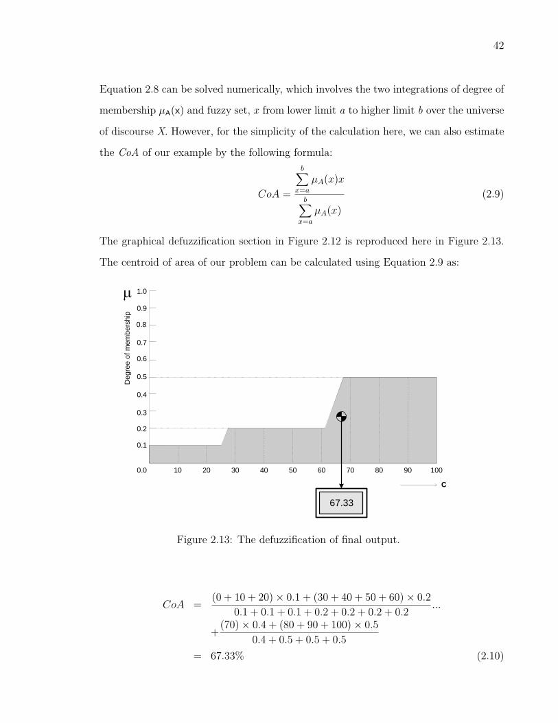
42

Equation 2.8 can be solved numerically, which involves the two integrations of degree of

membership µA(x) and fuzzy set, x from lower limit a to higher limit b over the universe

of discourse X. However, for the simplicity of the calculation here, we can also estimate

the CoA of our example by the following formula:

CoA =

b∑x=a

µA(x)x

b∑x=a

µA(x)

(2.9)

The graphical defuzzification section in Figure 2.12 is reproduced here in Figure 2.13.

The centroid of area of our problem can be calculated using Equation 2.9 as:

Deg

ree

of m

embe

rshi

p

0.0

0.2

0.5

0.4

0.3

0.1

0.6

0.7

0.8

0.9

1.0

10 20 30 40 50 60 70 80 90 100

67.33

C

µ

Figure 2.13: The defuzzification of final output.

CoA =(0 + 10 + 20)× 0.1 + (30 + 40 + 50 + 60)× 0.2

0.1 + 0.1 + 0.1 + 0.2 + 0.2 + 0.2 + 0.2...

+(70)× 0.4 + (80 + 90 + 100)× 0.5

0.4 + 0.5 + 0.5 + 0.5

= 67.33% (2.10)

43

The calculated CoA through Equation 2.10 is the final FLC output, that is in the form

of a crisp number. We begin in the inference analysis in step 1 with the crisp number

of inputs, and now we end it with the FLC output in the form of crisp number too. In

between, the fuzziness of sets has been exploited to arrive at this point. Finally back

to our example stated in the last paragraph in Step 1, the FLC has determined the

appropriate throttle setting for a given flying condition. That is, the throttle open is

67.33% for still air of 35% and target altitude of 60%.

2.6.6 Scaling Factors, Tuning, and Evaluation

Usually, designers are more interested in having fuzzy logic controllers that are independent

of physical domain of the variables. By having this, the designed FLC is not limited to one

particular problem, and thus offers greater flexibility. This independence of physical domain

can be achieved by normalizing the membership functions within [-1, +1] as mentioned in

[74, 48], or it means to have the range on the universe of discourse within [-1, +1]. An

important aspect is that the inputs and outputs values have to be scaled to fit the normalized

universe of discourse. Although the mapping of inputs and outputs using scaling factors are

linear, it has a strong impact on the performance of the controller because the scaling factors

directly influence the value of the open-loop gain coefficient [74].

These scaling factors are subjected to the tuning process, which is the last part in

building a fuzzy system. Tuning the scaling factors is quite difficult, and takes much more

time and effort than choosing fuzzy sets, membership functions, and constructing the rules.

Usually, reasonable scaling factors can be achieved after a series of tests. In general, the tasks

to evaluate and tune the fuzzy system are to examine whether the built fuzzy subsystems

meet the requirements specified at the beginning. Tuning and evaluating a fuzzy system may

involve any of the following [79, 80, 65, 64, 73, 66]:

• Review input and out variables, if required redefine their ranges.

• Review the fuzzy sets, and if required to define additional sets on the universe of dis-

44

course.

• Review the shapes of membership functions (fuzzy sets). However, in most cases, the

fuzzy systems are highly tolerant of a shape approximation, and thus a system can still

behave well even when the shapes of fuzzy sets are not precisely defined.

• Adjust the inputs and outputs scaling factors.

• Adjust the rule base in terms of their number and the chosen antecedent and consequent.

2.7 SUMMARY

This chapter has justified the necessity to have a VTOL UAV that is small, ducted-fan type,

and has high speed capability to successfully perform close range ISR missions. It was found

that the conventional approaches to control the highly complex and nonlinear ducted-fan

UAV are not sufficient. An intelligent control approach based on fuzzy logic was found to

have a special characteristic which is able to some extend, to replicate how humans make

decisions. The foundation of fuzzy logic has been laid out, including steps needed in building

an autonomous controller based on this approach.

45

Chapter 3

CONFIGURATION, AERODYNAMIC,

AND PROPULSION

3.1 INTRODUCTION

A new configuration of a small ducted-fan UAV is presented here, which is a response towards

several issues discussed in the preceding chapter. Some design considerations, important

design elements, and specialties related to the proposed UAV are highlighted. Then we

discuss the estimation of the aerodynamic properties of the vehicle, followed by the design

and analysis of control surfaces. The estimation of the UAV’s propulsion will also be provided,

where we will discuss the power required in all flight phases, the generation of thrust from

the fan and the duct, and the possible type of powerplant.

3.2 VEHICLE CONFIGURATION

In this study, a new configuration of a UAV is proposed, known as the DUAV (Ducted-fan

Unmanned Aerial Vehicle). The novelty of this vehicle is that it combines several features from

the following configurational varieties: rotorcraft, conventional airplane, tail-sitter vehicles,

and ducted fan UAV. The rationale of establishing most of the outstanding features from

these flying vehicles on a single UAV design is mainly to improve weaknesses of one and

another. Based on the aimed application areas, and in response to the both advantages and

disadvantages of existing UAVs discussed in Chapter 2, a new UAV configuration is proposed

as shown in Figure 3.1. It is a VTOL and ducted-fan type, with two rectangular wings, and

has a cruciform tail configuration.

The fuselage of the vehicle is formed by a blunted cylinder fore body that is elongated

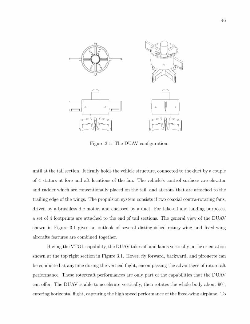
46

Figure 3.1: The DUAV configuration.

until at the tail section. It firmly holds the vehicle structure, connected to the duct by a couple

of 4 stators at fore and aft locations of the fan. The vehicle’s control surfaces are elevator

and rudder which are conventionally placed on the tail, and ailerons that are attached to the

trailing edge of the wings. The propulsion system consists if two coaxial contra-rotating fans,

driven by a brushless d.c motor, and enclosed by a duct. For take-off and landing purposes,

a set of 4 footprints are attached to the end of tail sections. The general view of the DUAV

shown in Figure 3.1 gives an outlook of several distinguished rotary-wing and fixed-wing

aircrafts features are combined together.

Having the VTOL capability, the DUAV takes off and lands vertically in the orientation

shown at the top right section in Figure 3.1. Hover, fly forward, backward, and pirouette can

be conducted at anytime during the vertical flight, encompassing the advantages of rotorcraft

performance. These rotorcraft performances are only part of the capabilities that the DUAV

can offer. The DUAV is able to accelerate vertically, then rotates the whole body about 90o,

entering horizontal flight, capturing the high speed performance of the fixed-wing airplane. To

47

land, the DUAV performs a reverse maneuver, and descends smoothly to the ground. During

the entire flight mission, the vehicle can repeatedly perform the transition manoeuvres in

both ways as frequently as required. A further discussion on the DUAV flights is given in

Chapter 5. In the following section, several design considerations related to the DUAV are

discussed.

3.2.1 Design Considerations

In general, there are two basic problems in the airplane design [81]: (1) given an airplane,

what are the performance, stability, and control characteristics?, and (2) given performance,

stability, and control characteristic, what is the airplane?. This thesis is more concerns with

the first problem, although in several design aspects, decisions are made to ensure the vehicle

behaves in specific ways. A new UAV conceptual design configuration is proposed, shown in

Figure 3.1, that employs conventional control surfaces mounted behind the fan duct. The fan

exit flow provides dynamic pressure at the tail for the control surfaces to function in hover

and low speed. Two small wings are mounted on the duct to provide lift in horizontal flight..

As discussed in Section 2.3, a ducted-fan is beneficial in many ways: extra thrust, lift

generator, reduces noise, extra space for components, and increases safety. An interesting

fact is that the interaction between the wing and duct produces a lift larger than the sum

of lift produced from each individual component. More interestingly, this effect increases in

magnitude with airspeed [82]. However, these advantages can only be grasped if the shape of

the duct is properly designed. Otherwise, it only adds to the weight penalty.

Another important design aspect is the shape of the duct lip. Since the vertical flight

is operated at low Reynolds number, the vehicle shape and a wide range of α causes the

aerodynamic effects to be strongly nonlinear and involves flow separation [24]. At high α,

the windward duct lip could experience separated flow. Inappropriate shape of the duct lip

could cause this separated flow to get into the fan, which in turn causes the lift and pitching

moment to suddenly reduce to the point where the pitching moment reverses sign. This is

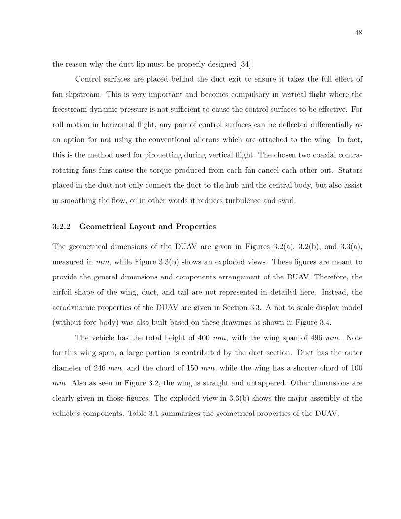
48

the reason why the duct lip must be properly designed [34].

Control surfaces are placed behind the duct exit to ensure it takes the full effect of

fan slipstream. This is very important and becomes compulsory in vertical flight where the

freestream dynamic pressure is not sufficient to cause the control surfaces to be effective. For

roll motion in horizontal flight, any pair of control surfaces can be deflected differentially as

an option for not using the conventional ailerons which are attached to the wing. In fact,

this is the method used for pirouetting during vertical flight. The chosen two coaxial contra-

rotating fans fans cause the torque produced from each fan cancel each other out. Stators

placed in the duct not only connect the duct to the hub and the central body, but also assist

in smoothing the flow, or in other words it reduces turbulence and swirl.

3.2.2 Geometrical Layout and Properties

The geometrical dimensions of the DUAV are given in Figures 3.2(a), 3.2(b), and 3.3(a),

measured in mm, while Figure 3.3(b) shows an exploded views. These figures are meant to

provide the general dimensions and components arrangement of the DUAV. Therefore, the

airfoil shape of the wing, duct, and tail are not represented in detailed here. Instead, the

aerodynamic properties of the DUAV are given in Section 3.3. A not to scale display model

(without fore body) was also built based on these drawings as shown in Figure 3.4.

The vehicle has the total height of 400 mm, with the wing span of 496 mm. Note

for this wing span, a large portion is contributed by the duct section. Duct has the outer

diameter of 246 mm, and the chord of 150 mm, while the wing has a shorter chord of 100

mm. Also as seen in Figure 3.2, the wing is straight and untappered. Other dimensions are

clearly given in those figures. The exploded view in 3.3(b) shows the major assembly of the

vehicle’s components. Table 3.1 summarizes the geometrical properties of the DUAV.

49

496.0

400.0

276.0

100.0

112.0

90.0

80.0

170.0

(a)

276.0

90.0

R60

400.0

220.0

115.0

125.0

130.0

20.0

(b)

Figure 3.2: The DUAV: (a) Front view, (b) Right view.

50

276.0

246.0

216.0

15.0

15.0

125.0

496.0

(a)

RMIT University

SCALE:1:2

SIZE DWG. NO.

AREV.

MATERIAL

FINISH

--

--

DO NOT SCALE DRAWINGAPPLICATION

USED ONNEXT ASSY

DIMENSIONS ARE IN INCHES

TOLERANCES:

FRACTIONAL

ANGULAR: MACH BEND

TWO PLACE DECIMAL

THREE PLACE DECIMAL

NAME DATE

DRAWN

CHECKED

ENG APPR.

MFG APPR.

Q.A.

SHEET 1 OF 1WEIGHT:

COMMENTS:

THE INFORMATION CONTAINED IN THIS

DRAWING IS THE SOLE PROPERTY OF

<INSERT COMPANY NAME HERE>. ANY

REPRODUCTION IN PART OR AS A WHOLE

WITHOUT THE WRITTEN PERMISSION OF

<INSERT COMPANY NAME HERE> IS

PROHIBITED.

PROPRIETARY AND CONFIDENTIAL Explode View

DUAV

Crosstail Assy

Rotor

Wings

Duct/pod/stators

Fuselage/stators

(b)

Figure 3.3: The DUAV: (a) Top view, (b) Exploded view.

51

Figure 3.4: A display model of the DUAV.

Table 3.1: Geometrical reference for the DUAV.

Parameter Value Parameter Value

Wing span 0.250 m Tail sweep angle 14o

Wing chord 0.100 m Tail taper ratio 0.9

Duct inner dia. 0.216 m Elevator area 0.005 m2

Duct outer dia. 0.246 m Rudder area 0.005 m2

Duct chord 0.150 m Aileron area 0.002 m2

Tail chord 0.112 m Tail span 0.276 m

Fan dia. 0.212 m Fore body dia. 0.06 m

3.2.3 Mass and Inertia Properties

The total mass, or conveniently referred as weight of the vehicle was estimated based on the

weight contributions from each component. These components are grouped into the following:

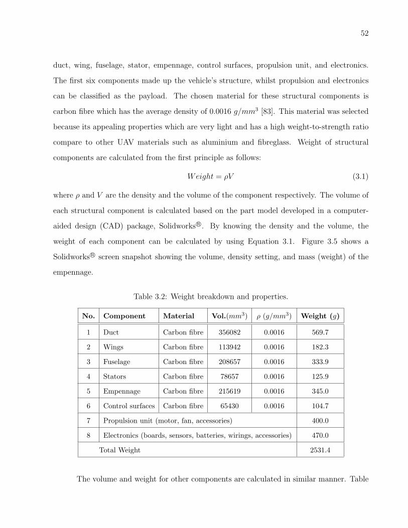
52

duct, wing, fuselage, stator, empennage, control surfaces, propulsion unit, and electronics.

The first six components made up the vehicle’s structure, whilst propulsion and electronics

can be classified as the payload. The chosen material for these structural components is

carbon fibre which has the average density of 0.0016 g/mm3 [83]. This material was selected

because its appealing properties which are very light and has a high weight-to-strength ratio

compare to other UAV materials such as aluminium and fibreglass. Weight of structural

components are calculated from the first principle as follows:

Weight = ρV (3.1)

where ρ and V are the density and the volume of the component respectively. The volume of

each structural component is calculated based on the part model developed in a computer-

aided design (CAD) package, Solidworks R©. By knowing the density and the volume, the

weight of each component can be calculated by using Equation 3.1. Figure 3.5 shows a

Solidworks R© screen snapshot showing the volume, density setting, and mass (weight) of the

empennage.

Table 3.2: Weight breakdown and properties.

No. Component Material Vol.(mm3) ρ (g/mm3) Weight (g)

1 Duct Carbon fibre 356082 0.0016 569.7

2 Wings Carbon fibre 113942 0.0016 182.3

3 Fuselage Carbon fibre 208657 0.0016 333.9

4 Stators Carbon fibre 78657 0.0016 125.9

5 Empennage Carbon fibre 215619 0.0016 345.0

6 Control surfaces Carbon fibre 65430 0.0016 104.7

7 Propulsion unit (motor, fan, accessories) 400.0

8 Electronics (boards, sensors, batteries, wirings, accessories) 470.0

Total Weight 2531.4

The volume and weight for other components are calculated in similar manner. Table

53

Figure 3.5: Volume and weight calculation for empennage.

3.2 shows the list of all components, together with their volume, density, and weight break-

down of the total vehicle’s weight. The weight of the propulsion system assembly, which

include all related components such as motor, fan, spinner, gears, and accessories is esti-

mated directly as 400 g. The basis of this estimation is that most of the propulsion system

components are readily available as off-the-shelves components. For example, a brushless DC

motor with the rating of 900 watts (1.2 hp) is commercially available, and weighs only 235 g

[84].

This 1.2 hp electric motor is good enough for DUAV since the typical motor power

rating for small UAVs is only around 0.8 hp [85]. The detail estimation of the power required

for DUAV is available in Section 3.4.1. For the electronics, the total weight is estimated as 470

g. It was estimated heavier than the propulsion system because it contains more components

such as controller boards, batteries, sensors, cameras, wirings, and accessories. Propulsion

system and electronics components with their estimated weights are added to the complete

assembled model as shown in Figure 3.6.

54

Figure 3.6: The assembled model of the DUAV.

Then, the primary moment of inertia for the vehicle are calculated based on this

assembled model. The moment of inertia of a solid body is defined as the sum of products of

masses of each elementary particle and the square of their distance from the given axis [83].

If dm represents the mass of an elementary particle and r is its distance from an axis, the

moment of inertia, I of the body about this axis is given as:

I =∫r2dm (3.2)

The integration of the square distance to obtain the moment of inertia as shown in Equation

3.2 is done numerically in Solidworks R©. A screen snapshot showing the primary moment of

inertia of the DUAV is depicted in Figure 3.7. Note in this figure that the reference axis

system has different axes directions compare to the standard reference axis system used to

develop the vehicle dynamics in Chapter 4. For convenience, the moment of inertia calculated

in Solidworks R© shown in Figure 3.7 are reproduced in Table 3.3 in terms of standard axis

system used in flight mechanics, where x-axis points forward, y-axis points starboard, and

55

z-axis points downward, all have the origin at the center of gravity.

Figure 3.7: Calculation of moment of inertia for the DUAV.

Table 3.3: Mass and inertia properties for the DUAV.

Parameter Value

Mass 2.5 kg

Ix 0.05 kgm2

Iy 0.05 kgm2

Iz 0.06 kgm2

Ixz 0 kgm2

56

3.2.4 Vehicle Specialty and Missions

The DUAV is designed to meet demanding characteristics that are lacking or unavailable in

the existing UAVs. In Section 2.4, we have highlighted several ducted-fan UAVs that have

received a lot of attention, yet none of those UAVs are built to meet all crucial mission

requirements either in military or civilian applications. Therefore, the DUAV is developed

to offer several added values to the existing UAVs which can be thought as a package that

meets all the following requirements:

• Fly faster more than 100 km/h: The ability of the DUAV to transit into horizontal flight

(airplane mode) indicates this vehicle has the potential to gain a high speed flight like

a typical fixed-wing airplane. Simulation result in Section 6.9 shows this is achievable.

• A VTOL technology : It is very clear that this vehicle takes full advantage of VTOL

capabilities. The placement of four control surfaces at the fan wake makes the control

during VTOL mode possible without a separate control system inside the duct.

• Small and compact with the maximum 2.5 kg gross weight : The DUAV is designed in

a relatively small size and compact in order to fit in several missions as outlined in

Section 2.3.

• Simple configuration: This vehicle is adopting a simple configuration in terms of one

control mechanism for both VTOL and horizontal flight modes, the propulsion, and the

airframe.

• Autonomous control : A fully autonomous control is developed, with the option of semi

and remote control as discussed in Chapter 5.

• Simple controller : By using fuzzy logic, a simple, quick, and effective controller is

designed as discussed in Chapter 5.

• Easily transportable: Since the size of the DUAV is very small, it is very convenient to

carry this vehicle by an operator to virtually all places for take-off.

57

By acquiring all these characteristics, the DUAV is very well suited to perform close range

ISR missions within 1 km to 5 km flight range. The ability to hover and land in small areas

makes the DUAV valuable for “perch and stare” missions. It may land in an area of interest,

shut down the engine, and it becomes a stationary sensor platform. An additional advantage

of being able to fly faster in the airplane mode enables the DUAV to accomplish the mission

in a shorter time.

3.3 AERODYNAMIC

The aerodynamic of the DUAV is very complex because of its unusual configuration, and due

to the fact that this vehicle was determined to fly in two flights regions that are contradicting

in requirements. In a low-speed vertical flight, the motion and control of the DUAV depend

only on the thrust and fan slipstream over elevator and rudder. Whereas, in high speed

horizontal flight, the aerodynamic behaviour is mainly dominated by the freestream dynamic

pressure. In addition, there is significant aerodynamic interference between fan and duct

[86]. Traditionally, the aerodynamic behaviour of a newly developed aircraft is determined

experimentally through wind tunnel and flight tests. However, this can be a slow process

that may involve equipment scheduling, data analysis, planning and executing flight tests,

whereas all these tasks are not practical in the early design process. With respect to this, a

quick method to estimate the aerodynamic properties of this UAV has been used.

Aerodynamic analysis was performed to estimate the DUAV characteristic that is

necessary to develop the non-linear simulation. Aerodynamic coefficients used for DUAV

simulation were calculated using theoretical methods [87], which makes extensive use of the

U.S Air Force Stability and Control Data Compendium (DATCOM) [88]. The theoretical

method to estimate aerodynamic properties that is described in [87, 88] provides systematic

steps in estimating preliminary aerodynamic stability and control derivatives of an aircraft

before it is actually built.

The method uses a large collection of aircraft design data, that is collected from ex-

58

tensive wind tunnel tests. From these correlated wind tunnel tests data, numerous general

formulations were derived that can be used to determine various parameters of a new aircraft

configuration. It provides graphical and analytical techniques to predict how various param-

eters such as aircraft geometry, mass, and inertia properties affect non-dimensional control

and stability derivatives of the aircraft.

Here, the calculation of aerodynamic properties should be regarded as a preliminary

step that gives an insight into the flight characteristics of this new UAV design. A disadvan-

tage of this method is that it lacks accuracy. Nevertheless, this weakness is accounted for in

the design of flight controller in Chapter 5. Aerodynamic properties of each geometric part

of the DUAV were calculated individually. Then, the aerodynamic contributions from all

parts are summed together, resulting in the total aerodynamic coefficient for the vehicle [32].

Aerodynamic interaction effects between vehicle’s parts are quantified, where such effects are

dominant. Approximation has been made in several sections to reduce the complexity of the

analysis as the referred method is mainly developed for conventional airplane configurations.

3.3.1 Aerodynamic Coefficients

The aerodynamic model of the DUAV is developed from an analysis that is restricted to two

dimensional, subsonic, and steady incompressible flow. This restriction simplifies the aerody-

namic analysis and is a reasonable assumption for small aircraft flying below Mach 0.4 [89].

The rudimentary principles in the generation of aerodynamic forces and moments is based

on Bernoulli’s equation and continuity principle of incompressible fluids. The aerodynamic

forces and moments expressed in terms of non-dimensional aerodynamic coefficients are given

in Equations 3.3 to 3.8:

D = qSCD (3.3)

Y = qSCy (3.4)

L = qSCL (3.5)

l = qSbCl (3.6)

59

M = qScCM (3.7)

N = qSbCN (3.8)

where D, Y, L are drag, sideforce, and lift, while l, M, N are rolling, pitching, and yawing

moments respectively. S, b and c are the wing area, wing span, and wing mean aerodynamic

chord respectively. The term q is dynamic pressure given by 12ρV 2

T , where VT is the total

velocity of the vehicle. The total aerodynamic coefficients are usually consisting of a baseline

component, plus incremental or correction terms [90]. For subsonic flight, the baseline com-

ponent is primarily a function of α, and β. In this thesis, the components build up for force

and moment coefficients are expressed in Equations 3.9 to 3.14, which only include significant

derivatives to the flight motion [91].

CL = CLo + CLαα+ CLδeδe +

c

2VT(CLα

α+ CLqq) (3.9)

CD = Cd +(CL − CLo)

2

πeR(3.10)

CY = CYββ + CYδr

δr (3.11)

CM = CMo + CMαα+ CMδeδe +

c

2VT(CMα

α+ CMqq) (3.12)

Cl = Clββ + Clδaδa + Clδr

δr +b

2Va(Clpp+ Clrr) (3.13)

CN = CNββ + CNδr

δr +b

2VT(CNpp+ CNrr) (3.14)

All derivatives that appear in Equations 3.9 to 3.14 were estimated using theoretical methods

obtained from reference [87]. This method depends on a large collection of empirical and

experimental data developed over many years, and interpolations and extrapolations were

made as necessary. The applied equations are presented in the components build up form,

dictated in Equations 3.15 to 3.35. A description of all coefficients listed in Equations 3.15

to 3.35 is available in Appendix A. Basically, the calculation of a particular derivative is a

summation of all related vehicle components that contribute to the total magnitude of that

60

derivative.

CLα = CwbLα

+ CdLα

+ ChLαηh(Sh/S)(1− dε/dα) (3.15)

CMα = (dCM/dCL)CLα + CdMα

(3.16)

CMq = CwMq

+ ChMq

(3.17)

CLq = CwLq

+ ChLq

+ CvLq

(3.18)

CLδe= αδeC

ihL (3.19)

CMδe= Cih

Mαδe (3.20)

CYβ= Cw

Yβ+ Cf

Yβ+ Cv

Yβ(3.21)

Clβ = Cwflβ

+ Chlβ

+ Cvlβ

(3.22)

CNβ= Cw

Nβ+ Cf

Nβ+ Cv

Nβ(3.23)

Clp = Cwlp + Ch

lp + Cvlp (3.24)

CNp = CwNp

+ CvNp

(3.25)

Clr = Cwlr + Cv

lr (3.26)

CNr = CwNr

+ CvNr

(3.27)

Clδa= Claδa (3.28)

CYδr= Cv′

LαK ′bαδCL

C ′lδ (3.29)

Clδr= ((zvcosα− lvsinα)/b)CY δr (3.30)

CNδr= −CYδr

(lvcosα + zvsinα)/b (3.31)

CLo = CwfLo

+ ChLαηh(Sh/S)(−αhoL − εho) + Cd

Lo(3.32)

CMo = CwMo

+ CdMo

+ ChMo

(3.33)

Cd = Cwbd + Cpod

d + Cdd (3.34)

CLα= 2Ch

LαηhVh(dε/dα) (3.35)

Although the theoretical estimation has a limited accuracy, it is the only convenient way of

61

estimating aircraft parameters at the initial design stage [31, 32]. This theoretical method

is very useful at this stage as it gives an insight of the vehicle’s characteristic before a more

accurate methods such as CFD and wind tunnel test are conducted. Once these detailed

analyses and experiments are carried out, the result from these methods can be used to

validate the initial data obtained through the emperical methods.

This approach is well aligned with the process involved in designing a new aircraft,

where several stages of analyse have to be carried out which consists of a combination of

theoretical, computational, and experimental techniques [92]. In view that the proposed

UAV design is still at the preliminary stage, in this thesis it is sufficient to use the theoretical

approach in estimating the vehicle’s aerodynamic.

Referring again to the build-up expressions in Equations 3.15 to 3.35, there are several

derivatives that have more significant effect on the aerodynamic characteristics than the oth-

ers. For example, the most important derivative that gives a big contribution to the magnitude

of CL is the lift curve slope, CLα . In our case, it is not appropriate for the CLα calculation to

depend solely on the method suggested in [87]. This is because the suggested method for CLα

calculation is for wing-body configuration only, whereas the DUAV configuration consists of

a duct that also needs careful consideration.

In addition to the wing CLα predicted using method in [87], the CLα for the duct is

estimated based on empirical data of a similar group of ducts found in [93]. Here, wind tunnel

tests were carried out on five ducts which had equal projected areas but with varying aspect

ratios of 0.33, 0.67, 1.00, 1.5, and 3.0. The models were tested for a range of α from −4o

to 90o. This range of α was in line with the range of α for the DUAV in both vertical and

horizontal flights. Refer again to the general layout of the DUAV in Section 3.2.2, the aspect

ratio (AR) of the DUAV’s duct can be calculated as:

AR =dicd

=216.0 mm

150.0 mm= 1.44 (3.36)

where di and cd are duct inner diameter and chord respectively. Since the AR of the DUAV’s

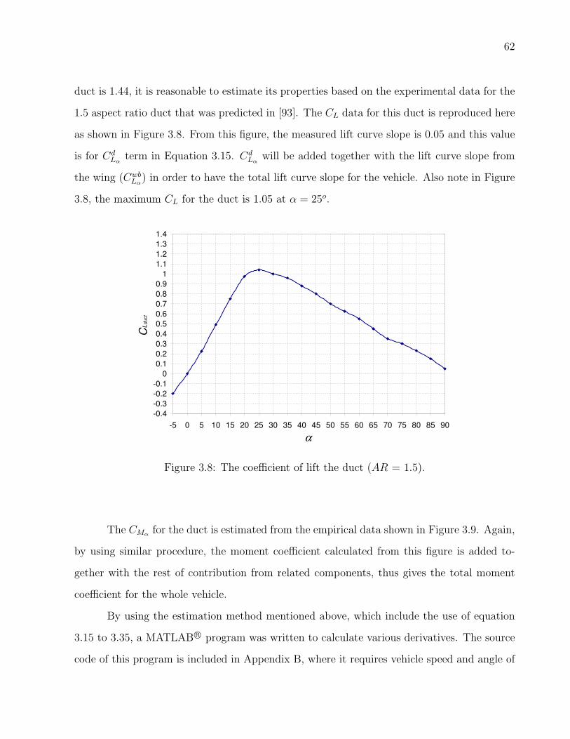
62

duct is 1.44, it is reasonable to estimate its properties based on the experimental data for the

1.5 aspect ratio duct that was predicted in [93]. The CL data for this duct is reproduced here

as shown in Figure 3.8. From this figure, the measured lift curve slope is 0.05 and this value

is for CdLα

term in Equation 3.15. CdLα

will be added together with the lift curve slope from

the wing (CwbLα

) in order to have the total lift curve slope for the vehicle. Also note in Figure

3.8, the maximum CL for the duct is 1.05 at α = 25o.

-0.4

-0.3

-0.2

-0.1

0

0.1

0.2

0.3

0.4

0.5

0.6

0.7

0.8

0.9

1

1.1

1.2

1.3

1.4

-5 0 5 10 15 20 25 30 35 40 45 50 55 60 65 70 75 80 85 90

α

CL

duct

Figure 3.8: The coefficient of lift the duct (AR = 1.5).

The CMα for the duct is estimated from the empirical data shown in Figure 3.9. Again,

by using similar procedure, the moment coefficient calculated from this figure is added to-

gether with the rest of contribution from related components, thus gives the total moment

coefficient for the whole vehicle.

By using the estimation method mentioned above, which include the use of equation

3.15 to 3.35, a MATLAB R© program was written to calculate various derivatives. The source

code of this program is included in Appendix B, where it requires vehicle speed and angle of

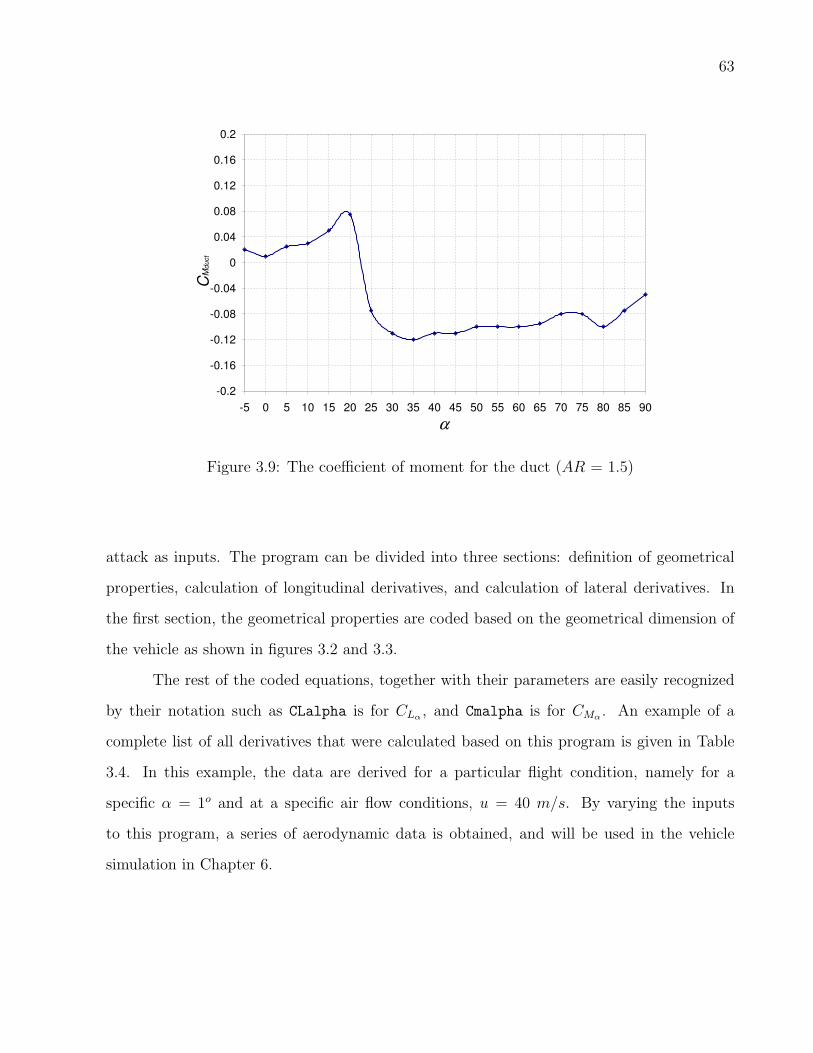
63

-0.2

-0.16

-0.12

-0.08

-0.04

0

0.04

0.08

0.12

0.16

0.2

-5 0 5 10 15 20 25 30 35 40 45 50 55 60 65 70 75 80 85 90

α

CM

duct

Figure 3.9: The coefficient of moment for the duct (AR = 1.5)

attack as inputs. The program can be divided into three sections: definition of geometrical

properties, calculation of longitudinal derivatives, and calculation of lateral derivatives. In

the first section, the geometrical properties are coded based on the geometrical dimension of

the vehicle as shown in figures 3.2 and 3.3.

The rest of the coded equations, together with their parameters are easily recognized

by their notation such as CLalpha is for CLα , and Cmalpha is for CMα . An example of a

complete list of all derivatives that were calculated based on this program is given in Table

3.4. In this example, the data are derived for a particular flight condition, namely for a

specific α = 1o and at a specific air flow conditions, u = 40 m/s. By varying the inputs

to this program, a series of aerodynamic data is obtained, and will be used in the vehicle

simulation in Chapter 6.

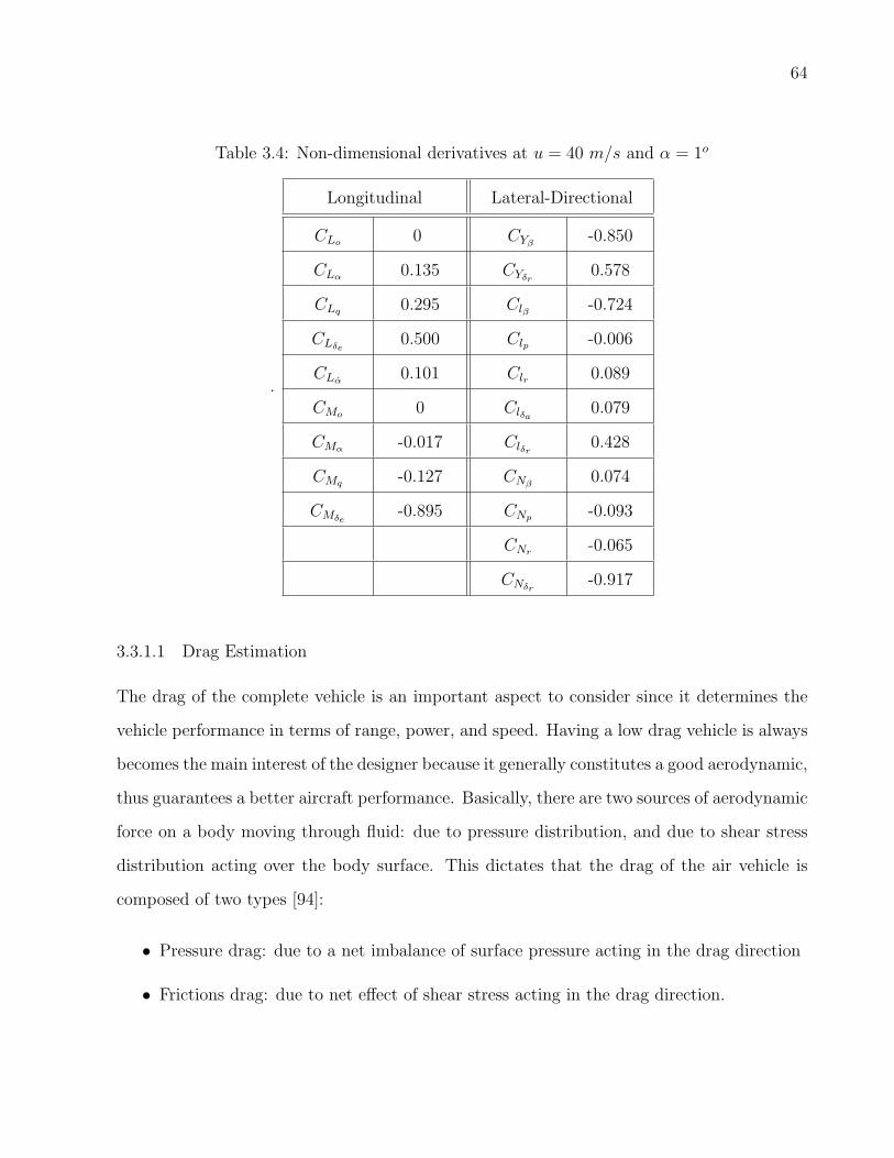
64

Table 3.4: Non-dimensional derivatives at u = 40 m/s and α = 1o

.

Longitudinal Lateral-Directional

CLo 0 CYβ-0.850

CLα 0.135 CYδr0.578

CLq 0.295 Clβ -0.724

CLδe0.500 Clp -0.006

CLα0.101 Clr 0.089

CMo 0 Clδa0.079

CMα -0.017 Clδr0.428

CMq -0.127 CNβ0.074

CMδe-0.895 CNp -0.093

CNr -0.065

CNδr-0.917

3.3.1.1 Drag Estimation

The drag of the complete vehicle is an important aspect to consider since it determines the

vehicle performance in terms of range, power, and speed. Having a low drag vehicle is always

becomes the main interest of the designer because it generally constitutes a good aerodynamic,

thus guarantees a better aircraft performance. Basically, there are two sources of aerodynamic

force on a body moving through fluid: due to pressure distribution, and due to shear stress

distribution acting over the body surface. This dictates that the drag of the air vehicle is

composed of two types [94]:

• Pressure drag: due to a net imbalance of surface pressure acting in the drag direction

• Frictions drag: due to net effect of shear stress acting in the drag direction.

65

The general breakdown of the total airplane drag is indicated in Equation 3.37 [95], where

Dp is the parasite drag, Di is the induced drag, and DS is the wave drag.

ΣD = Dp +Di +DS (3.37)

Dp, is composed of two parts: skin friction drag and pressure drag. The skin friction drag

is the result of shearing stress within a thin layer of the air as it passes over the surface of

the body. The pressure drag results from the imbalance in normal pressure forces around the

body due to the flow separation that normally occurred at high angle of attack [95]. The next

drag component, Di is pressure drag due to pressure imbalance in the drag direction caused

by the induced flow (downwash) associated with the vortices created at the tip of finite wings.

It can be modeled as:

CDi=

C2L

πeAR(3.38)

The last drag component, DS is due to the effect of shock wave (related to supersonic flow) on

the pressure distribution. However, this drag component is not relevant to the DUAV since

this vehicle is designed to fly at relatively low subsonic speed. Therefore, we can write the total

drag coefficient for the vehicle in the form as shown in Equation 3.10 (CD = Cd + (CL−CLo )2

πeR).

On the right hand side of this equation, the first coefficient term is parasite drag, while the

second term is induced drag. Here for the DUAV, Cd is the contribution from all components

which are wings, duct, fuselage, and tail. This can be written as,

Cd = Cwd + Cd

d + Cfd + Ct

d (3.39)

For the duct, the estimation of Cdd was also based on careful consideration of the

empirical data found in [93]. In this report, an experiment was done for a series of ducts that

have different aspect ratios. Figure 3.10 in an excerpt from [93] which shows the variation of

drag coefficient with α for a duct that has the aspect ratio of 1.5.

The result shown in this figure can be used as a guideline to estimate the total drag

for the DUAV’s duct. This is because the final DUAV configuration has the duct with the

66

0

0.1

0.2

0.3

0.4

0.5

0.6

0.7

0.8

0.9

1

1.1

1.2

1.3

1.4

0 5 10 15 20 25 30 35 40 45 50 55 60 65 70 75 80 85 90

α

CD

duct

Figure 3.10: The coefficient of drag for the duct (AR = 1.5).

aspect ratio of 1.44, which is very close to 1.5 as indicated in Equation 3.36. By using similar

procedure, the drag coefficient for the duct is added together with the rest of the Cd from

other vehicle’s components, thus forms the total drag coefficient for the whole vehicle.

Another source of preliminary drag estimation of the vehicle is found in [96]. Never-

theless, there is small difference in the vehicle configuration considered in this thesis with the

one that was considered in that report. The initial DUAV configuration without the extended

nose as shown in Figure 3.4 was selected. A typical result for CD that was obtained for the

unextended DUAV configuration is shown in Figure 3.11 [96].

Obviously, the extended nose configuration that is considered in this thesis, as shown in the

geometrical drawings in Figure 3.3 has a bigger surface area, therefore we can expect a higher

drag on this vehicle as shown in Figure 3.12.

67

Figure 3.11: Drag coefficient for initial UAV configuration.

0

0.25

0.5

0.75

1

1.25

1.5

1.75

2

2.25

2.5

2.75

3

0 5 10 15 20 25 30 35 40 45 50 55 60 65 70 75 80 85 90

α

CD

Figure 3.12: The coefficient of drag for the DUAV.

3.3.1.2 Stators Design

The design of stators are done mainly for the following reasons: as support struts, for com-

ponents placement, and for aerodynamic purposes. While the first two reasons are clearly

understood, the last function of stators designed needs careful attention. For this purpose,

68

stators design has remove the resulting swirl from the flow so that the flow is straighten as

much as possible for maximum control surface effectiveness.

Swirl is an unwanted angular rotation of the flow and represents a form of energy loss,

that is part of the energy was used to accelerate the flow in the angular sense, rather in axial

direction to produce the thrust. The stators are usually arranged in radial orientation, so the

lateral components of the lift will cancel, resulting only in a torque and an axial force. Figure

3.13 shows the arrangement of four stators for the DUAV.

Stators Stators

Figure 3.13: Radial arrangement of stators.

3.3.1.3 Propeller Effects

For a propeller-driven airplane, the effects of power from propeller operation are generally

significant on the aerodynamic characteristic of the vehicle [97]. These effects are quite

substantial on the lift, pitching moment, drag, and elevator hinge moment. The propeller

slipstream over the wing, tail, and fuselage increases the dynamic pressure, swirl the airflow,

create downwash and sidewash at the tail, and negative dihedral effect at high angle of attack.

Although the DUAV is not considered as a conventional propeller-driven type aircraft, it has,

to some extent the resemblance of this effect, which is the fan slipstream over the cruciform

69

tail.

Interestingly, the control in vertical flight solely depends on the propeller effects (slip-

stream) on the tail, since the vehicle is flying at a very low freestream dynamic pressure.

However, in the horizontal flight, the propeller effect is quite obvious since it increases the

dynamic pressure over the tail, in addition to the freestream dynamic pressure due to the

high speed flight. Therefore, the calculation of the aerodynamic coefficients are different for

these two type of flights. At this moment, it is appropriate to consider the propeller effect

only caused the dynamic pressure to increase in horizontal flight. A detailed treatment of the

slipstream effect over the control surfaces is among the topics discussed in the next section.

3.3.2 Control Surfaces Design

There are a few options of the control surface design that can be considered. The chosen

design must offer the best solution to the problem at hand. All moving control vanes have

the advantage that it can eliminate hinge moment [37]. However, it is difficult and complicated

to be integrated with the design arrangement of four points landing footprints. Conventional

ailerons are ineffective in vertical flight due to low dynamic pressure in the external flow field.

The reaction control jets and cyclic pitch propeller are too complex for this type of UAV. The

best solution is to design the control surfaces that can benefit from the fan slipstream at all

flight phases, and at the same time entails a simple design layout.

This is the main reason for the selected four control surfaces placed on the cruciform

tail, that immersed in the duct outflow. The design of control surfaces is relatively simple,

and to some extent, it resembles the elevator and rudder arrangements on a typical fixed-

wing aircraft. Figure 3.14 shows the arrangement of control surfaces on the DUAV. These

four control surfaces or flaps can be deflected in several schemes, in order to have vehicle

control in both vertical and horizontal flights. Also note in the figure that the conventional

ailerons attached to the wings are for the roll control in horizontal flight only.

Refer to Figure 3.14(a), flaps 1 and 3 are deflected downward (δ1 and δ3) to give pitch

70

1δ

3δ 2δ

4δ

ZB

YB

(a) Bottom view of flaps

ZB

XB XB

YB

1δ2δ 3δ4δ

(b) Side and front views of flaps

Figure 3.14: Control surfaces arrangement of the DUAV.

control about YB-axis. In this deflection scheme, flaps 1 and 3 can be regraded as the elevator,

δe. The upward and downward deflection schemes of flap 1 and 3 are also used to control

LSTF motions in the vehicle’s belly directions (backward and forward). Similarly, flaps 2 and

4 are deflected symmetrically in order to have yaw control about ZB-axis. In this case, flaps

2 and 4 are function as a rudder, δr. In vertical flight, symmetrical deflection scheme of flaps

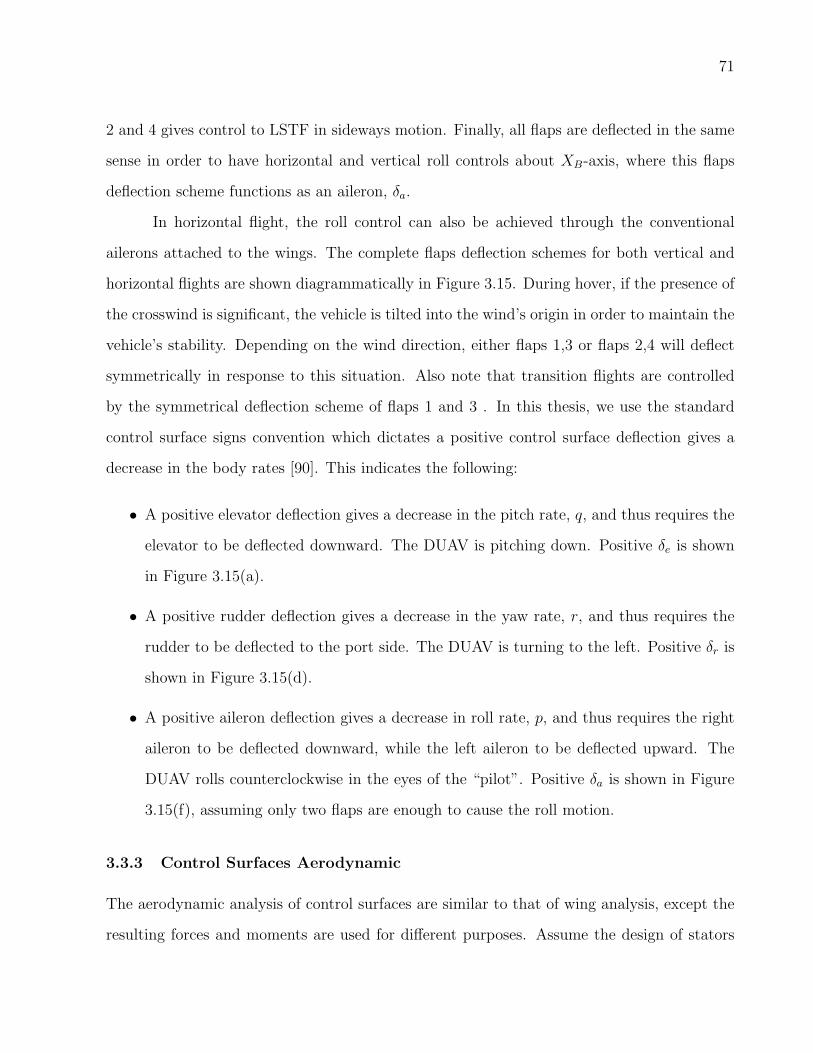
71

2 and 4 gives control to LSTF in sideways motion. Finally, all flaps are deflected in the same

sense in order to have horizontal and vertical roll controls about XB-axis, where this flaps

deflection scheme functions as an aileron, δa.

In horizontal flight, the roll control can also be achieved through the conventional

ailerons attached to the wings. The complete flaps deflection schemes for both vertical and

horizontal flights are shown diagrammatically in Figure 3.15. During hover, if the presence of

the crosswind is significant, the vehicle is tilted into the wind’s origin in order to maintain the

vehicle’s stability. Depending on the wind direction, either flaps 1,3 or flaps 2,4 will deflect

symmetrically in response to this situation. Also note that transition flights are controlled

by the symmetrical deflection scheme of flaps 1 and 3 . In this thesis, we use the standard

control surface signs convention which dictates a positive control surface deflection gives a

decrease in the body rates [90]. This indicates the following:

• A positive elevator deflection gives a decrease in the pitch rate, q, and thus requires the

elevator to be deflected downward. The DUAV is pitching down. Positive δe is shown

in Figure 3.15(a).

• A positive rudder deflection gives a decrease in the yaw rate, r, and thus requires the

rudder to be deflected to the port side. The DUAV is turning to the left. Positive δr is

shown in Figure 3.15(d).

• A positive aileron deflection gives a decrease in roll rate, p, and thus requires the right

aileron to be deflected downward, while the left aileron to be deflected upward. The

DUAV rolls counterclockwise in the eyes of the “pilot”. Positive δa is shown in Figure

3.15(f), assuming only two flaps are enough to cause the roll motion.

3.3.3 Control Surfaces Aerodynamic

The aerodynamic analysis of control surfaces are similar to that of wing analysis, except the

resulting forces and moments are used for different purposes. Assume the design of stators

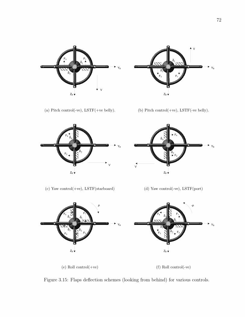
72

1δ

3δ

ZB

YB

F1F3

V

(a) Pitch control(-ve), LSTF(+ve belly).

1δ

3δ

ZB

YB

F1F3

V

(b) Pitch control(+ve), LSTF(-ve belly).

2δ

4δ

ZB

YB

F2

F4

V

(c) Yaw control(+ve), LSTF(starboard)

2δ

4δ

ZB

YB

F2

F4

V

(d) Yaw control(-ve), LSTF(port)

1δ

3δ2δ

4δ

ZB

YB

p

F1

F2

F4

F3

(e) Roll control(+ve)

1δ

3δ

2δ

4δ

ZB

YB

-p

F1

F2

F4

F3

(f) Roll control(-ve)

Figure 3.15: Flaps deflection schemes (looking from behind) for various controls.

73

as discussed in Section 3.3.1.2 are able to cancel the swirl completely, then all flaps are

encountering a perfect slipstream effect at any time. This is to ensure all flaps have sufficient

dynamic pressure (that results from the fan slipstream), so that these control surfaces are

constantly effective. The forces and moment that act on the DUAV are shown in Figure

3.16(a), where it also depicts the slipstream path over the flaps. Then in Figure 3.16(b), it

shows how to resolve the forces for a flap submerged in the fan slipstream. Note in Figure

3.16, the local angle of attack and pitch angle of the flap are denoted as αf and θf respectively.

α

T

W

XB

M

L

DV

Fan slipstream

Flap

ZB

(a) (b)

Figure 3.16: Fan slipstream over flaps: (a) Forces and moments on the body, (b) Forces actingon a flap.

The effective velocity of the slipstream, Veff over the flap’s surface is defined as:

Veff = Va + vi (3.40)

where the axial velocity, Va depends on the forward speed of the vehicle, V and the angle of

attack, α. Refer both Figures 3.16(a) and 3.16(b), the axial velocity can be determined as

74

follows:

Va = V cosα (3.41)

The induced velocity, vi can be derived by using momentum theory of the airflow into the

duct, and is given by Equation 3.42, where ρ is the freestream density, and A is the fan disc

area.

vi =

√T

2ρA(3.42)

Now we can calculate the total dynamic pressure around the flap, q, as shown in Equation

3.43.

q =1

2ρV 2

eff

q =1

2ρ(Va + vi)

2 (3.43)

In this slipstream model, no account is taken for the possibility of mixing the slipstream with

other external flows. While this is indefensible due to the viscosity of the air, it is beyond the

scope of the present work to estimate such effect. However, it is quite reasonable to have this

assumption since flaps are closely located behind the duct exit. Since the operating Mach

number is so small, the slipstream is considered steady and incompressible. We also assume

that the slipstream axis is coincident with the fan axis, thus the induced velocity is perfectly

straight downstream. Now we derive the useful force of the flap that is due to the slipstream.

Refer back to Figure 3.16(b), as the fan increases the axial velocity Va, it also imparts a

tangential velocity component to the flow (Vt), that is given by:

Vt =1

2Ωr (3.44)

where Ω is the rotational speed of the fan, and r is the radial position on the fan blade. By

75

having this and using vi given in Equation 3.42, the swirl velocity, Vs is determined, and in

consequence, the flap pitch angle, θf and the angle of attack, αf are also obtained. The total

lift coefficient of the flap, CLFis computed from

CLF=

Nf∑1

(CfLαδf ) (3.45)

where Nf is number of flaps, and CfLα

is the flap lift curve slope calculated from the Equation

3.46 obtained in [87].

CfLα

=2πkARf

2 +

√AR2(1−M2)

k2

[1 +

tan2(Λ0.5cf)

1−M2

]+ 4

(3.46)

where M is the Mach number, ARf is aspect ratio of the flap, and Λ0.5cf is the sweep ratio

at the flap half-chord (0.5cf ). The tan(Λ0.5cf ) expression is given by,

tan(Λ0.5cf ) = tan(ΛLEf)− 1

ARf

1− λ

1 + λ(3.47)

where the flap taper ratio, λ = cfr/cft , with subscript r and t indicate the flap chord at the

root and at the tip respectively. For our case that is ARf ≤ 4, the correction factor k in

Equation 3.46 is given by:

k = 1 +(1.87− 0.000233ΛLEf

)ARf

100(3.48)

By inserting Equations 3.46 to 3.48, into Equation 3.45, the total lift coefficient of the flap,

CLfis obtained. Next we estimate the drag of the flap, Cf

D: consists of drag due the lift or

induced drag, CfDi

, and skin friction drag, Cfd .

CfD = Cf

Di+ Cf

d (3.49)

Since the flap is treated as a wing, the induced drag stated is Equation 3.38 is also applied to

76

the flap, and is reproduced here with the addition of subscript f to indicate this expression

is for flap.

CfDi

=C2Lf

πARfef(3.50)

where ef is the flap span efficiency factor. The skin friction drag on the flap is estimated

using an expression found in [98] as follows:

Cfd = Cpf

[1 +G(t/c)fmax + 100((t/c)fmax)

4]RLS × SWf

/Sf (3.51)

where the constant, Cpf = 0.064/Re2, and Re is the Reynolds number. SWf/Sf is the ratio

of flap wetted area to flap area, and (t/c)fmax is the maximum flap thickness to chord ratio.

The factor G and lift surface factor RLS are calculated by using Equation 3.52 and Equation

3.53 respectively.

G =

1.2 for (t/c)fmax at x ≥ 0.3cf

2.0 for (t/c)fmax at x < 0.3cf

(3.52)

RLS = 1.6598− 6.0017cosΛ(t/c)fmax

+ 13.314cos2Λ(t/c)fmax

−10.932cos3Λ(t/c)fmax

+ 3.0303cos4Λ(t/c)fmax

(3.53)

Substituting Equations 3.50 to 3.53 into Equation 3.49, we obtained the total drag coefficient

for the flap, CfD. Back to Figure 3.16(b), forces on the flap are determined by lift and drag

of the flap, and its pitch angle, θf . We can represent these forces in terms of a component

perpendicular to (CfX), and a component parallel to (Cf

Y ) the fan rotation plane as follows:

CfX = Cf

L(sinθf − (Df/Lf )cosθf (3.54)

CfY = Cf

L(cosθf − (Df/Lf )sinθf (3.55)

It is assumed that each flap is producing equal amount of lift and drag, therefore, it is also

77

producing the equal amount of CfY . Examining closely Figure 3.16, the Cf

Y force component

that we just have derived is the most useful force obtained from the flap. This is the force

that gives controls to the vehicle, and as we have discussed, various flap deflection schemas

can be used either to transfer these force components into a total resultant force, or into an

effective moment.

3.4 PROPULSION

The propulsion of the DUAV is to meet the thrust requirement for flying in both VTOL

and airplane modes. Basically, more thrust is needed in the VTOL flying mode since it is

the only source of lift to sustain the vehicle’s weight, and also to cause the vehicle to fly

in the directional plane. We begin with the estimation of power required, derivation of the

fan’s thrust, followed by the discussion of the thrust due to the duct’s shape, and finally the

derivation of thrust available from the selected brushless d.c motor.

3.4.1 Power Estimation

The estimation of power required at all flight modes is essential because it enables us to select

the appropriate powerplant for the vehicle. As we have noted, the flight envelope of DUAV

composes of vertical flight, transition flight, and horizontal flight. Fundamentally, the power

required in any flight is given by multiplying the vehicle’s velocity through the air with the

thrust. In steady flight, the thrust is required to balance all forces that oppose the motion.

Since the vehicle has to accelerate in some parts of the flight, the available power from the

thrust generator should be in excess of the powered needed in steady flight.

In vertical flight, the thrust is required to overcome vehicle’s weight and drag. As

discussed in Section 3.2.3, the estimated total weight of the DUAV is 2.5 kg. Also, as

suggested in the initial study of the DUAV found in [5], an estimate of 3 N drag in vertical

flight is reasonable. Therefore, the thrust needed to balance the DUAV’s weight and drag in

78

vertical flight can be written as,

Tv = mg + drag

= 2.5kg × 9.81m/s2 + 3N = 27.5N (3.56)

The DUAV is designed to have a moderate rate of climb around 8 m/s. However, if

the DUAV needs to perform vertical to horizontal maneuver, it has to accelerate vertically

beyond this velocity. As mentioned earlier, this maneuver is needed to enable the vehicle enter

the high speed flight region. This means at the moment the vehicle initiates this maneuver,

which is in vertical mode, the current vertical speed must be close enough to the high speed

wing-borne flight. This is to ensure a smooth transition from thrust-supported vertical flight

to duct and wing-supported horizontal flight. From the initial aerodynamic analysis of DUAV

found in [99], at the velocity of 25 m/s, the wing and duct start to effective. This draws a

conclusion that the estimation of power required in vertical flight must take into account this

maximum vertical velocity. Therefore, the power can be calculated as,

Pwd = TvVv

= 27.5N × 25m/s

= 687.5W (3.57)

The induced power due to the induced velocity should be included in the calculation of the

total power required in vertical flight. The induced velocity in vertical flight is given as [100],

vi,v = −0.5Vv + vh√

(Vv/2vh)2 + 1 (3.58)

where Vv and vh are vertical climb velocity and hover induced velocity respectively. The

relationship between induced velocity, exit velocity, and thrust at hover is,

Thvh =1

2mV 2

e (3.59)

79

where subscript h refers to hover. The exit velocity Ve is equal to 2vh. This will be derived

later in Section 3.4.2, where the result is shown in Equation 3.79. Insert this relationship into

Equation 3.59 yields,

Thvh =1

2m(2vh)

2

Th = 2mvh (3.60)

Substitute the air mass flow rate, m = ρAfvh in Equation 3.60, and simplify the equation for

hovering induced velocity,

Th = 2ρAfvhvh

vh =

√Th

2ρAf(3.61)

The thrust required to hover is equal to the vehicle’s weight. The fan’s area, Af can be

calculated from the fan’s data given in Table 3.1. The air density is given as, ρ = 1.225

kg/m3. Thus, from Equation 3.61, the induced velocity for hover is,

vh =

√√√√ 2.5kg × 9.81m/s2

2× 1.225kg/m3 × π(0.106m)2

= 16.8m/s (3.62)

The power required to hover is calculated as,

Ph = Thvh

= 2.5kg × 9.81m/s2 × 16.8m/s

= 412.0W (3.63)

Then, the induced velocity in vertical flight can be calculated from Equation 3.58, with the

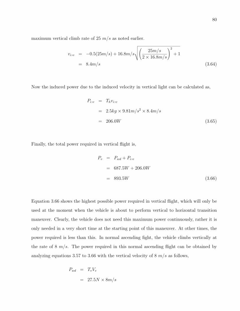
80

maximum vertical climb rate of 25 m/s as noted earlier.

vi,v = −0.5(25m/s) + 16.8m/s

√√√√( 25m/s

2× 16.8m/s

)2

+ 1

= 8.4m/s (3.64)

Now the induced power due to the induced velocity in vertical light can be calculated as,

Pi,v = Thvi,v

= 2.5kg × 9.81m/s2 × 8.4m/s

= 206.0W (3.65)

Finally, the total power required in vertical flight is,

Pv = Pwd + Pi,v

= 687.5W + 206.0W

= 893.5W (3.66)

Equation 3.66 shows the highest possible power required in vertical flight, which will only be

used at the moment when the vehicle is about to perform vertical to horizontal transition

maneuver. Clearly, the vehicle does not need this maximum power continuously, rather it is

only needed in a very short time at the starting point of this maneuver. At other times, the

power required is less than this. In normal ascending fight, the vehicle climbs vertically at

the rate of 8 m/s. The power required in this normal ascending flight can be obtained by

analyzing equations 3.57 to 3.66 with the vertical velocity of 8 m/s as follows,

Pwd = TvVv

= 27.5N × 8m/s

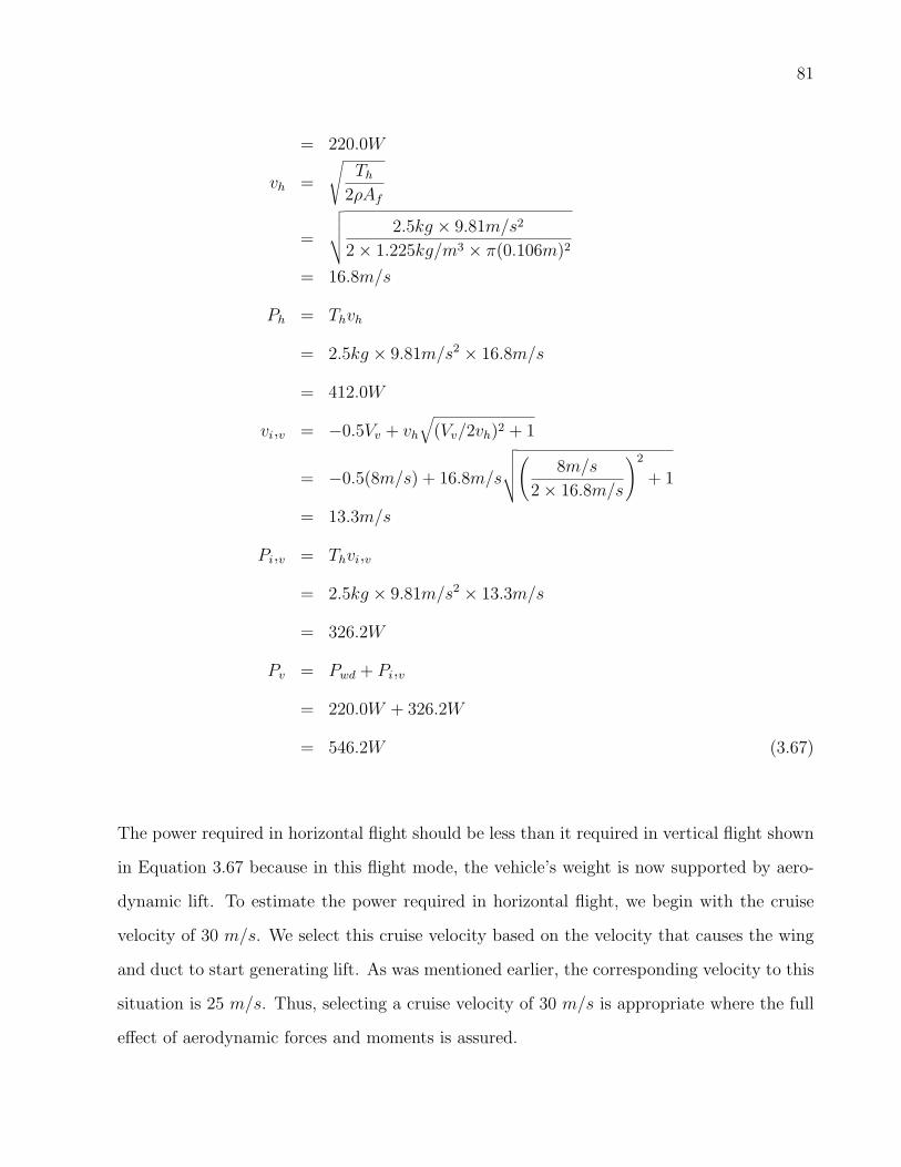
81

= 220.0W

vh =

√Th

2ρAf

=

√√√√ 2.5kg × 9.81m/s2

2× 1.225kg/m3 × π(0.106m)2

= 16.8m/s

Ph = Thvh

= 2.5kg × 9.81m/s2 × 16.8m/s

= 412.0W

vi,v = −0.5Vv + vh√

(Vv/2vh)2 + 1

= −0.5(8m/s) + 16.8m/s

√√√√( 8m/s

2× 16.8m/s

)2

+ 1

= 13.3m/s

Pi,v = Thvi,v

= 2.5kg × 9.81m/s2 × 13.3m/s

= 326.2W

Pv = Pwd + Pi,v

= 220.0W + 326.2W

= 546.2W (3.67)

The power required in horizontal flight should be less than it required in vertical flight shown

in Equation 3.67 because in this flight mode, the vehicle’s weight is now supported by aero-

dynamic lift. To estimate the power required in horizontal flight, we begin with the cruise

velocity of 30 m/s. We select this cruise velocity based on the velocity that causes the wing

and duct to start generating lift. As was mentioned earlier, the corresponding velocity to this

situation is 25 m/s. Thus, selecting a cruise velocity of 30 m/s is appropriate where the full

effect of aerodynamic forces and moments is assured.

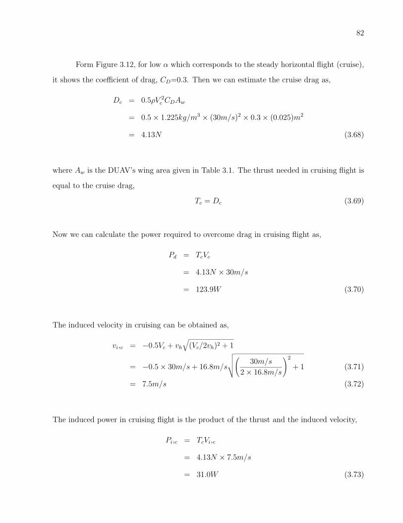
82

Form Figure 3.12, for low α which corresponds to the steady horizontal flight (cruise),

it shows the coefficient of drag, CD=0.3. Then we can estimate the cruise drag as,

Dc = 0.5ρV 2c CDAw

= 0.5× 1.225kg/m3 × (30m/s)2 × 0.3× (0.025)m2

= 4.13N (3.68)

where Aw is the DUAV’s wing area given in Table 3.1. The thrust needed in cruising flight is

equal to the cruise drag,

Tc = Dc (3.69)

Now we can calculate the power required to overcome drag in cruising flight as,

Pd = TcVc

= 4.13N × 30m/s

= 123.9W (3.70)

The induced velocity in cruising can be obtained as,

vi,c = −0.5Vc + vh√

(Vc/2vh)2 + 1

= −0.5× 30m/s+ 16.8m/s

√√√√( 30m/s

2× 16.8m/s

)2

+ 1 (3.71)

= 7.5m/s (3.72)

The induced power in cruising flight is the product of the thrust and the induced velocity,

Pi,c = TcVi,c

= 4.13N × 7.5m/s

= 31.0W (3.73)

83

Finally, we can estimate the total power required in cruising flight as follows,

Pc = Pd + Pi,c

= 123.9W + 31.0W

= 154.9W (3.74)

Until this far, we have estimated the power required in the following flights: hover, normal

ascend, maximum ascend, and horizontal cruising flight. Although in vertical mode, the

vehicle may perform various maneuvers such as tilted flight and pirouette, the power required

in these motions is not much different than is required for hover. Moreover, we can deduce

qualitatively that the descending flight requires much less power than is required for ascending

flight.

For horizontal flight, the power required is calculated at a typical cruising speed of 30

m/s. If the vehicle is required to cruise at a bit higher speed, it should not be a problem

since excessive power was estimated at the maximum speed of ascending flight. Therefore,

the analysis of power required that was presented above is sufficient to avoid the power to be

underestimated. Table 3.5 summarizes the power required for all flight modes.

Table 3.5: Estimation of power required.

Flight Power (W)

Hover 412.0

Normal Ascend 546.2

Maximum Ascend 893.5

Cruise 154.9

84

3.4.2 The Thrust

As described in Section 2.3, the duct can increase the static thrust produced by the fan. Let’s

consider Figure 3.17 which shows the airflow through a duct, where four important regions

are indicated (1 to 4). Region 1 is located at a distance far above the fan where the air in this

region is not affected by the fan. Region 2 is located just in front of the fan, while region 3 is

located just after the fan. Finally, region 4 is located far behind the fan. Note that because

region 4 is located far behind the fan, static pressures at this point and at point 1 are the

same. The airflow region in the duct is known as slipstream. Our analysis to estimate the

thrust from the fan is based on the momentum theory.

1

2

3

4

Vi

Ve

Vo

Af

Ae Po

Tf

Po

Figure 3.17: The airflow through the ducted-fan.

The fan is approximated by an infinitely thin actuator disc where a pressure change

occurs just before and after the disc, but it is uniformed over the disc. The air velocity is

also assumed to be steady over the disc. The thrust produced by the fan is equal to the mass

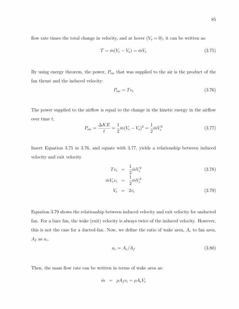
85

flow rate times the total change in velocity, and at hover (Vo = 0), it can be written as:

T = m(Ve − Vo) = mVe (3.75)

By using energy theorem, the power, Pow that was supplied to the air is the product of the

fan thrust and the induced velocity:

Pow = Tvi (3.76)

The power supplied to the airflow is equal to the change in the kinetic energy in the airflow

over time t,

Pow =∆KE

t=

1

2m(Ve − Vo)

2 =1

2mV 2

e (3.77)

Insert Equation 3.75 in 3.76, and equate with 3.77, yields a relationship between induced

velocity and exit velocity

Tvi =1

2mV 2

e (3.78)

mVevi =1

2mV 2

e

Ve = 2vi (3.79)

Equation 3.79 shows the relationship between induced velocity and exit velocity for unducted

fan. For a bare fan, the wake (exit) velocity is always twice of the induced velocity. However,

this is not the case for a ducted-fan. Now, we define the ratio of wake area, Ae to fan area,

Af as ar.

ar = Ae/Af (3.80)

Then, the mass flow rate can be written in terms of wake area as:

m = ρAfvi = ρAeVe

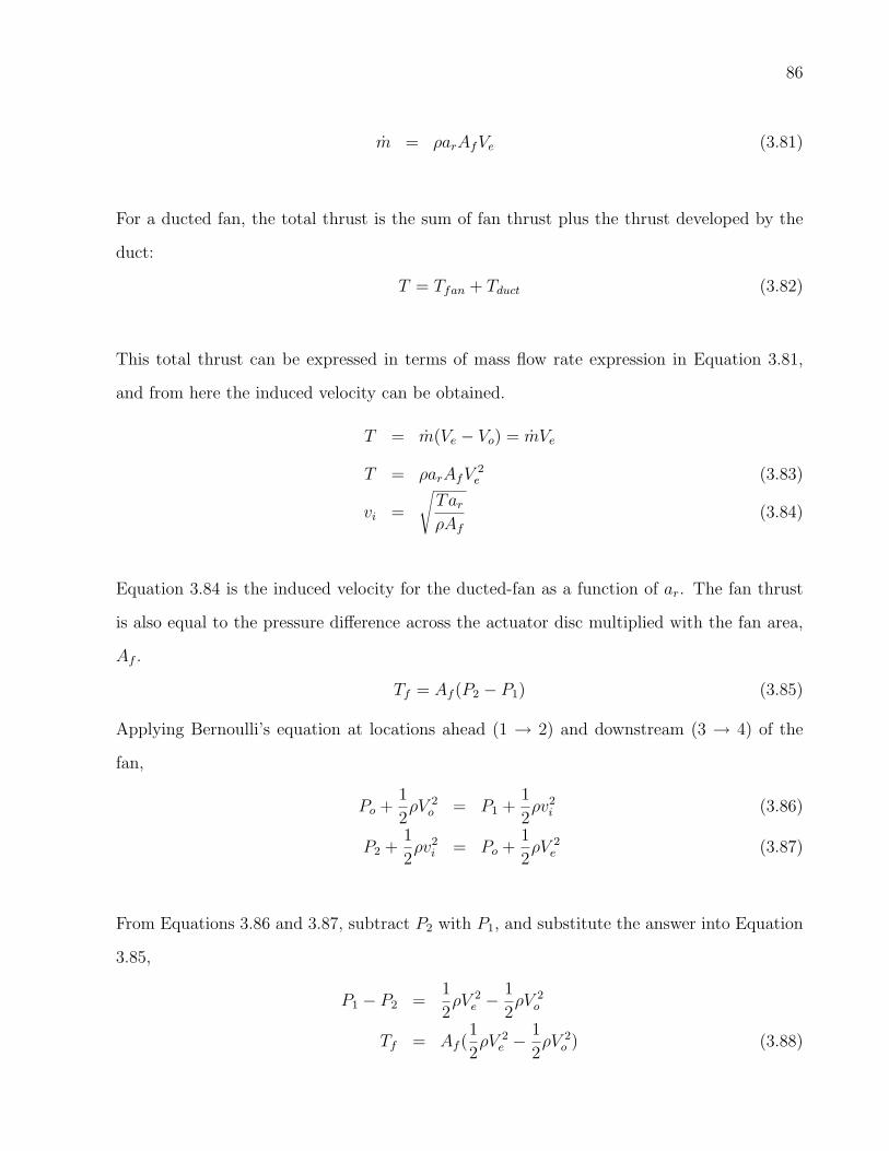
86

m = ρarAfVe (3.81)

For a ducted fan, the total thrust is the sum of fan thrust plus the thrust developed by the

duct:

T = Tfan + Tduct (3.82)

This total thrust can be expressed in terms of mass flow rate expression in Equation 3.81,

and from here the induced velocity can be obtained.

T = m(Ve − Vo) = mVe

T = ρarAfV2e (3.83)

vi =

√TarρAf

(3.84)

Equation 3.84 is the induced velocity for the ducted-fan as a function of ar. The fan thrust

is also equal to the pressure difference across the actuator disc multiplied with the fan area,

Af .

Tf = Af (P2 − P1) (3.85)

Applying Bernoulli’s equation at locations ahead (1 → 2) and downstream (3 → 4) of the

fan,

Po +1

2ρV 2

o = P1 +1

2ρv2

i (3.86)

P2 +1

2ρv2

i = Po +1

2ρV 2

e (3.87)

From Equations 3.86 and 3.87, subtract P2 with P1, and substitute the answer into Equation

3.85,

P1 − P2 =1

2ρV 2

e −1

2ρV 2

o

Tf = Af (1

2ρV 2

e −1

2ρV 2

o ) (3.88)

87

and at hover, Vo = 0, Equations 3.88 becomes,

Tf =1

2ρV 2

e Af (3.89)

Using Equation 3.83 and Equation 3.89, the ratio of fan thrust to the total thrust can be

written as:

TfT

=12ρV 2

e AfρarAfV 2

e

TfT

=1

2ar(3.90)

Using the thrust ratio in Equation 3.90, and the total thrust in Equation 3.82, and substitute

back ar, we can obtain the thrust due to the duct as follows:

Td = T − Tf

= Tf (2ar − Tf )

Td = Tf (2AeAf

− 1) (3.91)

Closely observe Equation 3.91, it deduces an important fact about the thrust developed by

the duct. It says, the thrust due to the duct is increased as the wake area, Ae increases.

This is the reason why the static thrust can be increased by shrouding the fan. However, by

simply ducting the fan without careful consideration of the duct shape will not necessarily

increase the static thrust. Usually, the divergent duct is used in order to increase the wake

area. The typical increment rate of 10% - 15% of the static thrust can be achieved by having

a ducted fan [101]. However, there is a physical limit to what extent the wake area can be

increased in order to have additional thrust. Excessive divergence of the duct could develop

flow separation at the duct exit which nullifies the duct induced effect.

88

The thrust estimation above shows the qualitative magnitude of the thrust when the

fan is shrouded. Comparatively, it was already shown that the static thrust of a ducted-fan

is higher compared to the same diameter of a bare fan. The increment of the thrust due to

the duct was also known as a function of wake area. Nevertheless, more detail about the

thrust is not available through momentum analysis. Therefore, a more useful information of

the fan thrust can be derived from blade element theory. Based on the blade element analysis

[95, 102], the thrust of the fan is:

T =∫ r=R

r=0b1

2ρ(Ωr)2a(θ − ϕ)cdr (3.92)

where b, ρ, a, θ, ϕ, c,Ω and R refer to number of fan blades, air density, fan blade lift coefficient,

blade pitch angle, inflow angle, blade chord, blade radius, and fan RPM respectively. For

simplicity of analysis, we assumed the inflow distribution is uniformed along the blade span,

and also the blade has an ideal twist. Therefore, for a constant chord blade (the chosen blade

for DUAV), the fan thrust can be written as:

T = CTπR2ρ(ΩR)2 (3.93)

where the thrust coefficient, CT and solidity ratio, σ are given as:

CT =σ

4a(θt − ϕt) (3.94)

σ = bc

πR (3.95)

where subscript t refers to the corresponding angle value at the blade tip. The torque of the

fan can be written as:

Q = CQπR2ρ(ΩR)2R (3.96)

89

where the torque coefficient, CQ is given as:

CQ =C

3/2T√2

+ σδ

8(3.97)

with δ here is referring to blade profile drag coefficient.

3.4.3 Model of Brushless D.C Motor

In Section 3.4.1, we have estimated the power required in all flight modes. Then in Section

3.4.2 we have discussed how thrust and torque for a given fan are calculated, and the cor-

responding equations are derived as given in Equations 3.93 and 3.96 respectively. Then in

this section we need to select the engine that will drive the fan and is is able to produce

power at the required level. When compared to the internal combustion engine, the electric

motor gives several advantages such as less noise and vibration, clean, easy handling, not

inflammable, and maintains the vehicle’s weight.

On the other hand, there are also a few disadvantages of using an electric brushless

motor such as it may require more weight and space for batteries, and gives a shorter flight

time. A trade off is needed in these conflicting factors. Because of the advantages stated

above, and a less difficult analysis is offered when the vehicle’s weight is fixed throughout

the flight, a brushless d.c motor is selected as the DUAV’s powerplant. In these days, the

technology of brushless d.c motors has advanced significantly until electrical motors that are

powerful, compact, rugged, and light are commercially available.

We provide an example of a series of Neumotors R© brushless d.c motors [84] that are

potentially capable to match the DUAV’s requirements as depicted in Figure 3.18. From

Table 3.5, it can be seen that the highest power required is 893.5 W . The best motor

that can produce this much power is probably 1907-1400 model, which is able to generate

continuous power of 900 W , and it can surge until double (1800 W ). However, the lower

motor model such as 1905-2060 is also enough to power the DUAV since the maximum 893.5

W is not continuously required. Even when this maximum power is required, the motor is

90

able to have the power surge of 1200 W , a rate that is more than enough. Amazingly, these

two motors weigh only 8.3 oz (235 g) and 6.4 oz (181 g) respectively.

Figure 3.18: Neumotors R© DC brushless motor data.

Refer to the vehicle’s weight estimation in Section 3.2.3, the weight range of these motors

is agreed with the allocated weight for the propulsion system. An important finding at this

point is that there are several brushless d.c motors available in the market that can match

the weight constraint and power demand of the DUAV. The analysis on detail matters such

as batteries selection, power consumption, and maximum run time are beyond the scope of

this thesis. However, it is necessary to discuss how an electric motor is able to produce useful

output, which is the torque. Theoretically, the torque produced by the motor can be modeled

as [103],

Tm = Kt(Vi/Rm − Io)(1− (Kt/Vi)Ω) (3.98)

where Kt is the torque constant, Vi in the input voltage, Rm is the motor resistance, and

Io is the input current. In this study, the control of the throttle, δth is merely equal to the

control of the input voltage. The combination of a fan and an electric motor can be viewed

as a propulsion unit. This propulsion unit has a good fan-motor match if both are operating

91

closely at their maximum efficiency. Examine closely the torque expressions in Equations 3.96

and 3.98, to have a good fan-motor matching, the efficiency curves of both fan and motor

should have their peaks at roughly the same rotational speed, Ω.

0 1 2 3 4 5 6 7 8 9 10 11 120

1000

2000

3000

4000

5000

6000

RP

M

δth

(v)

0 500 1000 1500 2000 2500 3000 3500 4000 4500 5000 5500 60000

8

16

24

32

40

48

Th

rust (N

RPM)

Figure 3.19: Throttle setting, RPM, and thrust model.

Since the detail performance data of Neumotors R© motors is inaccessible for research

purpose, it is sufficient at this moment to develop a simple but realistic propulsion model

in terms of a throttle-RPM-thrust relationship as shown in Figure 3.19. This model was

developed by considering the equation for fan thrust as given in 3.93, motor torque as given

in Equation 3.98, the augmented thrust due to the duct, and the available brushless d.c

motor to produce the power required. The performance data given in Figure 3.19 is used in

92

the flight control simulation in this study. A constraint is placed on the maximum available

thrust which is 48 N at δth = 12 V .

3.5 SUMMARY

The newly designed UAV is expected to be able to address the current problems faced by

existing UAVs in close range ISR missions. The vehicle, known as the DUAV integrates

several important design elements from rotorcraft, tail-sitter, ducted-fan, and fixed-wing air

vehicles. Critical design features of the vehicle were discussed which include the aerodynamic

design of stators that overcome fan’s torque, and the aerodynamic behaviour of the control

surfaces. The aerodynamic derivatives were estimated by using theoretical methods, where

a computer program was developed to manage the calculations. The propulsion model of

the vehicle was presented that includes the estimation of power required, the derivation of

fan thrust and augmented thrust from the duct, and the selection of a suitable commercially

available brushless d.c motor. Most of the data derived in this chapter will be used for the

simulation in Chapter 6.

93

Chapter 4

VEHICLE DYNAMICS

4.1 INTRODUCTION

This chapter begins with the definition of various axis systems used for DUAV dynamics

modeling and simulation. The equations of motion of the rigid body vehicle are derived from

Newton’s laws, and the attitude of the vehicle will be described. Then, the transformation

between axes are explained, and from here the kinematics and navigational equations are

developed. The components that made up the dynamics equations are discussed and the

method to solve the vehicle dynamics is presented.

4.2 AXIS SYSTEMS DEFINITION

The fact that the aircraft has six degrees of freedom to describe its motions makes the vehicle

dynamics problem becomes relatively complex. Three degrees of freedom are required to

define translational motions, while the other three are for rotational motions. Therefore,

motion is normally described by several variables which are related to chosen axis systems.

Thus it is necessary to define axis systems used in this subject.

4.2.1 Body-Axis System

The body-axis system designated by (XB, YB, ZB) in Figure 4.1 has the origin which usually,

but not necessarily, coincident with the aircraft center of gravity. It is a right-handed reference

frame that has the XB-axis positive out the nose of the aircraft, and the YB-axis is positive

to the right wing. The ZB-axis is positive normal to XBYB plane and points vertically

downward when the aircraft is in level flight. In most cases, the XBZB is the only aircraft

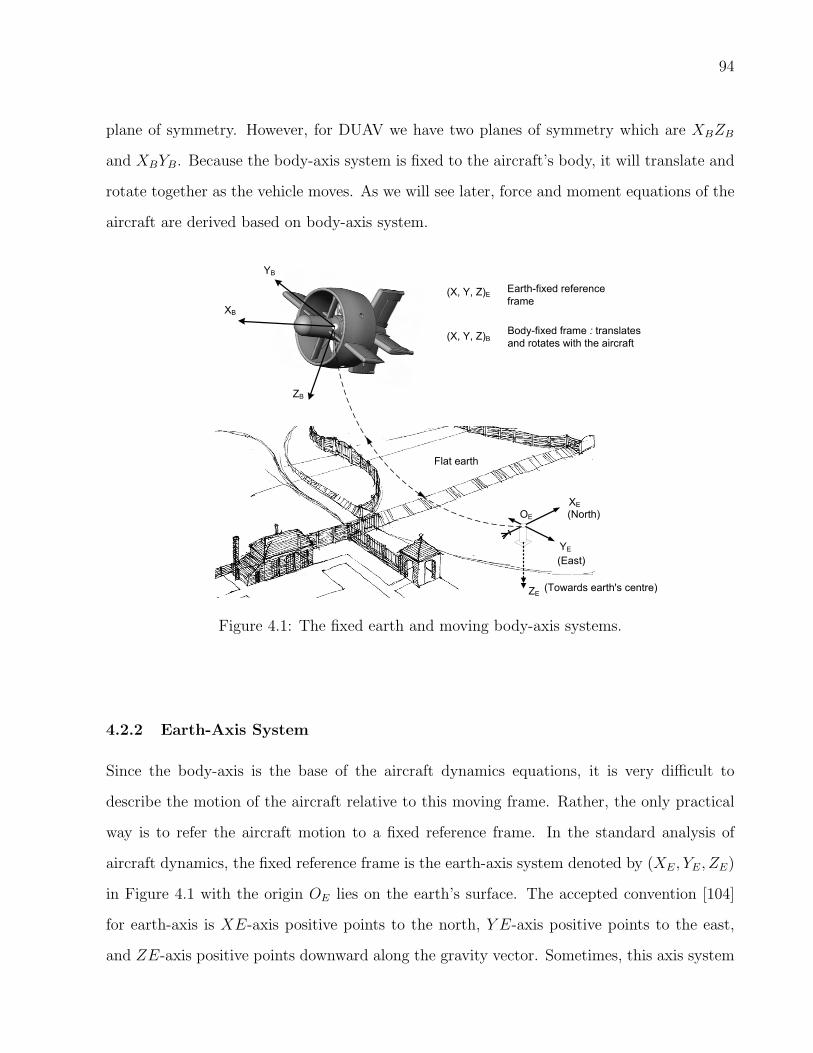
94

plane of symmetry. However, for DUAV we have two planes of symmetry which are XBZB

and XBYB. Because the body-axis system is fixed to the aircraft’s body, it will translate and

rotate together as the vehicle moves. As we will see later, force and moment equations of the

aircraft are derived based on body-axis system.

(North)

XB

ZB

YB

ZE

XE

YE

(East)

(X, Y, Z)E

(X, Y, Z)B

Earth-fixed reference

frame

Body-fixed frame : translates

and rotates with the aircraft

Flat earth

OE

(Towards earth's centre)

Figure 4.1: The fixed earth and moving body-axis systems.

4.2.2 Earth-Axis System

Since the body-axis is the base of the aircraft dynamics equations, it is very difficult to

describe the motion of the aircraft relative to this moving frame. Rather, the only practical

way is to refer the aircraft motion to a fixed reference frame. In the standard analysis of

aircraft dynamics, the fixed reference frame is the earth-axis system denoted by (XE, YE, ZE)

in Figure 4.1 with the origin OE lies on the earth’s surface. The accepted convention [104]

for earth-axis is XE-axis positive points to the north, Y E-axis positive points to the east,

and ZE-axis positive points downward along the gravity vector. Sometimes, this axis system

95

is also referred to as north-east-down (NED) axes. Here, we adapt the common inertial

coordinate system which is the Cartesian non-rotating earth-axis to be the fixed reference

frame.

4.2.3 Stability and Wind Axis Systems

The stability-axis is constructed from the body-axis system by a left-handed rotation through

α, around the body y-axis, as can be seen in Figure 4.2. It is used to analyze the effect of

perturbations from steady-state flight [105]. Imagine when the forward direction of the body

x-axis coincides with the velocity vector, then the body-axis system is referred to as stability-

axis. In the stability-axis system, the x-axis is maintained in the xBzB longitudinal plane.

If the aircraft is flying with sideslip, then stability-axis is now referred to as the wind-axis

system. Figure 4.2 depicts this resulting wind-axis, when the stability-axis rotates through β

around zB-axis. Normally, aerodynamic data obtained through wind tunnel tests is referred

in the wind-axis system.

4.3 EQUATIONS OF MOTION

Since the DUAV has a similar body-axis system with the conventional aircraft, the standard

six degrees of freedom aircraft equations of motion can be adopted. The rigid-body equations

of motion are derived from Newton’s second law of motion. The law states that the summa-

tion of all external forces acting on a body must be equal to the time rate of change of its

momentum, and the summation of all external moments acting on a body must be equal to

the time rate of change of its moment of momentum [106, 107, 108]. The law can be expressed

in time rates of change with respect to inertial space by the following vector equations,

∑F =

d

dt(mVc)

]E

(4.1)

∑M =

d

dt(H)

]E

(4.2)

96

Figure 4.2: Body, stability, and wind-axis systems.

where Vc represents the translational velocity of the aircraft,∑F represents the sum of all

externally applied forces,∑M represents the sum of all applied moments. The term mVc is

the linear momentum, whereas H is the moment of momentum or angular momentum of the

aircraft. In a very general scalar form, vector in Equation 4.1 consists of three force equations

as follows:

Fx =d

dt(mu), Fy =

d

dt(mv), Fz =

d

dt(mw) (4.3)

where Fx, Fy, Fz and u, v, w are force components and velocity components along x, y, and z

axes respectively. The components of moment can also be written as:

L =d

dt(Hx),M =

d

dt(Hy), N =

d

dt(Hz) (4.4)

97

where L, M,N andHx, Hy, Hz are the components of the moment, and moment of momentum

along x, y, and z axes respectively. In general, components of force and moment are composed

of contribution from aerodynamic, propulsive, and gravitational forces acting of the aircraft.

Figure 4.3 shows all components of velocity (u, v, w), force (Fx, Fy, Fz) , body rate (p, q, r),

and moment (L,M,N) in their positive sense. The positive sense of these variables are

determined by the right-hand rule. Also shown in the figure are Euler angles (φ, θ, ψ), which

will be explained later.

XB

ZB

YB

OB

L, p,

FX, uN, r,

φ

ψ

θ

FZ, w

FY, v

M, q,

Figure 4.3: The body-axis system of the DUAV.

The angular momentum of the rigid body aircraft, H is defined as:

H = Iω (4.5)

Here, ω is the angular velocity of the aircraft with respect to the earth-fixed axis system,

98

and I is the moment or product of inertia of the aircraft. When expressed in body-fixed

axis system, the velocities vector ω and Vc can be written as the sum of their corresponding

components with respect to XB, YB, ZB axes.

ω = pi + qj + rk (4.6)

Vc = ui + vj + wk (4.7)

The force and moment equations given in Equations 4.1 and 4.2 are referred to as non-rotating

earth-fixed axis system. In this case, as the aircraft rotates, moments and products of inertia

will vary with time which causes difficulty in the analysis. To solve this problem, we must

refer the force and moment vectors to the body-axis system. In general, the derivative of an

arbitrary vector A referred to a rotating body-axis frame, and having an angular velocity ω

can be represented by the following vector identity [109]:

dA

dt

]E

=dA

dt

]B

+ ω × A (4.8)

Applying this vector identity to the general form of force and moment expressions in Equations

4.1 and 4.2, gives force and moment expressions with respect to the body-axis system.

F =d

dt(mVc)

]B

+ ω × (mVc) (4.9)

M =d

dtH

]B

+ ω ×H (4.10)

Equations 4.9 and 4.10 that we have derived are the vector equations for general six degrees

of freedom motion. These equations are more commonly expressed in the scalar form which

offer more physical insight into aircraft motions. The scalar equations consist of six non-linear

differential equations of forces and moments as follows,

Fx = m(u+ qw − rv) (4.11)

99

Fy = m(v + ru− pw) (4.12)

Fz = m(w + pv − qu) (4.13)

L = Ixp+ (Iz − Iy)qr − Ixz(pq + r) (4.14)

M = Iy q + (Ix − Iz)pr + Ixz(p2 − r2) (4.15)

N = Iz r + (Iy − Ix)pq − Ixz(qr + p) (4.16)

Equations of motion given in Equations 4.11 to 4.16 are the central part of the DUAV sim-

ulation. These full six degrees of freedom nonlinear equations of motion are derived with

several assumptions. As long as the assumptions are maintained, these equations are valid to

represent the atmospheric aircraft motions [108, 110]. The assumptions made in deriving the

equations are:

• The reference earth-axis frame is fixed, flat, and non-rotating in the space.

• The mass of the aircraft remains constant with respect to time.

• The XZ plane is the aircraft plane of symmetry. For the DUAV, it also have a plane

of symmetry in the XY plane, therefore the product of Ixz is 0.

• The aircraft is a rigid body.

4.4 AIRCRAFT ATTITUDE AND POSITION

The orientation of aircraft in body-axis system, xb, yc, and zb, relative to earth-fixed system,

xE, yE, and zE, is described by performing three consecutive rotations of earth-fixed system

[111, 109, 112]. The three angular rotations defined by the right handed rotation about three

axes of a right handed axes system are known as Euler angles. In aircraft dynamics, they

are commonly denoted as ψ, θ, and φ, which represent the azimuth angle or heading, the

elevation angle or pitch attitude, and bank angle or roll attitude respectively. It is important

100

to note that the order of the three consecutive rotations must be observed in the following

manner: ψ → θ → φ.

0

ψ

φ

θX1

X2 X3

Y1 Y2

Y3

Z2 Z1

Z3

ψ

φθ

Y0

Z0

X0

(X1 , Y1 , Z1 ) First rotation

(X2 , Y2 , Z2 ) Second rotation

(X3 , Y3 , Z3 ) Third rotation

(X0 , Y0 , Z0 ) Original frame

Figure 4.4: The Euler angles rotations.

In the starting position, the vehicle body-axes are exactly aligned with the north-east-

down axes. Refer to Figure 4.4, first, rotate the earth-fixed frame about the z-axis through

an angle ψ. Next, rotate the revolved reference frame about the new y-axis through an angle

of θ. And finally, rotate the revolved reference frame about the new x-axis through an angle

φ, to arrive at the final body-axis reference frame [112]. These steps of revolving the axes

to define the aircraft orientation are illustrated in Table 4.1. The final rotation results in

the orientation of the aircraft relative to the earth-frame. Each Euler angle rotation and its

corresponding rotation matrix are shown in Table 4.1.

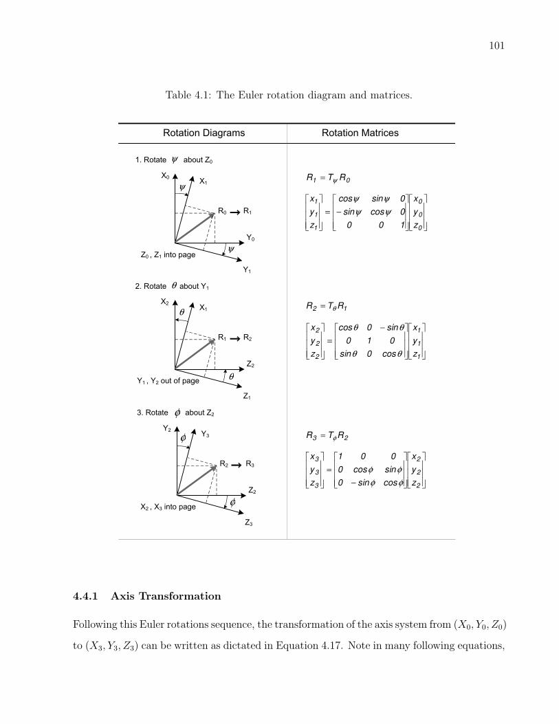
101

Table 4.1: The Euler rotation diagram and matrices.

Rotation Diagrams Rotation Matrices

−=

0

0

0

1

1

1

z

y

x

100

0cossin

0sincos

z

y

x

ψψ

ψψ

01 RTRψ

=

−

=

1

1

1

2

2

2

z

y

x

cos0sin

010

sin0cos

z

y

x

θθ

θθ

−

=

2

2

2

3

3

3

z

y

x

cossin0

sincos0

001

z

y

x

φφ

φφ

12 RTRθ

=

23 RTRφ

=

X0X1

Y0

Y1

ψ

R0 R1

ψ

1. Rotate about Z0 ψ

Z0 , Z1 into page

X2X1

Z2

Z1

R1 R2

2. Rotate about Y1θ

Y1 , Y2 out of page

Y2Y3

Z2

Z3

R2 R3

3. Rotate about Z2

X2 , X3 into page

θ

θ

φ

φ

φ

4.4.1 Axis Transformation

Following this Euler rotations sequence, the transformation of the axis system from (X0, Y0, Z0)

to (X3, Y3, Z3) can be written as dictated in Equation 4.17. Note in many following equations,

102

shorthand notations are used where Cos is written as C, and Sin is written as S.

T0⇒3 = TψTθTφ

=

Cψ Sψ 0

−Sψ Cψ 0

0 0 1

Cθ 0 −Sθ

0 1 0

Sθ 0 Cθ

1 0 0

0 Cφ Sφ

0 −Sφ Cφ

=

CθCψ CθSψ −Sθ

SφSθCψ − CφSψ SφSθSψ + CφCψ SφCθ

CφSθCψ + SφSψ CφSθSψ − SφCψ CφCθ

(4.17)

These three Euler rotations deduced an important transformation matrix that is useful to

transform variables from inertial frame to non-inertial frame. In our case, the inertial frame

is earth-axis system, and the non-inertial frame is body-axis system. The transformation

matrix T0⇒3 is called the direction cosine matrix (DCM). For convenience, we denote this

transformation matrix T0⇒3 as DCME⇒B, where the subscript indicates the transformation

from earth-axis (E) to body-axis (B). Transformation of virtually all variables from earth-axis

to body-axis is possible by using transformation matrix DCME⇒B.

DCME⇒B =

CθCψ CθSψ −Sθ

SφSθCψ − CφSψ SφSθSψ + CφCψ SφCθ

CφSθCψ + SφSψ CφSθSψ − SφCψ CφCθ

(4.18)

In general, say if we have two axes system: axis1 and axis2, the transformations between

them are formulated as follows:

[axis1

]=

[DCM

] [axis2

](4.19)[

axis2

]=

[DCM−1

] [axis1

](4.20)

To demonstrate the transformation from earth-axis to body-axis, suppose a vector ~vE in

103

earth-axis needs to be expressed in the body-axis ~vB. Then we must perform the following:

~vB

=

[DCME⇒B

] ~vE

(4.21)

vxB

vyB

vzB

=

CθCψ CθSψ −Sθ

SφSθCψ − CφSψ SφSθSψ + CφCψ SφCθ

CφSθCψ + SφSψ CφSθSψ − SφCψ CφCθ

vxE

vyE

vzE

(4.22)

This DCME⇒B will be used extensively in the vehicle simulation. Transformations of motion

variables and other flight parameters between axes are important in the study of aircraft

dynamics. Often, the aerodynamic coefficients or derivatives that were obtained through the

experimental investigation or computational analysis are computed based on the wind-axis

system. One of the reasons is the experimental setup, such as in a wind tunnel test, could be

done much easier if the direction of the free stream velocity coincides with the horizon.

In contrast, when we substitute these coefficients into equations of motion, the most

convenient way to solve the problem is to present all these equations in the body-axis system.

As such, another common axes transformation that is very useful is between stability axis and

body-axis system. Occasionally, the wind axis is also referred to as stability or aerodynamic

axes [104]. To maintain consistency, the term wind-axis is adopted throughout the text, and

the DCM required for transformation from body to wind axis is:

• Body to Wind Transformation

[DCMB⇒W

]=

CαCβ Sβ SαCβ

−CαSβ Cβ −SαSβ

Sα 0 Cα

(4.23)

The DCM for transformation from earth to body-axis can also be written in terms of quater-

nion parameters:

104

• Earth to Body Transformation (Quaternion)

[DCME⇒B

]=

e2x + e20 + e2y + e2z 2(exey + eze0) 2(exez + eye0)

2(exey + eze0) e2y + e20 + e2x + e2z 2(eyez + exe0)

2(exez + eye0) 2(eyez + exe0) e2z + e20 + e2x + e2y

(4.24)

4.4.2 Kinematic Equations

We have seen that the orientation of the aircraft at a specific time is determined by performing

three consecutive rotations of the earth-axis, provided the Euler angles: ψ, θ, and φ at that

specific time are available. Now it is necessary to derive differential equations that allow the

dynamics calculation of Euler angles. To begin with, it is good practice to superimpose the

angular rate vectors p, q, r on axes shown in Figure 4.4. The result of superimposing is shown

in Figure 4.5.

Euler rates vectors denoted in Figure 4.5 are also the result of three consecutive rota-

tions as described earlier, but here we have considered performing each of the rotation with

the corresponding angular rates ψ, θ, and φ. From Figure 4.5, we can establish relationships

between aircraft body rates and Euler rates, referred to datum axes as indicated in Equations

4.25 to 4.27 [104].

Roll rate, p = Σ of φ, θ, ψ components resolved along OX3

= φ− ψSθ (4.25)

Pitch rate, q = Σ of φ, θ, ψ components resolved along OY3

= θCφ+ ψSφCθ (4.26)

Yaw rate, r = Σ of φ, θ, ψ components resolved along OZ3

= ψCφCθ − θSφ (4.27)

105

Rearrange Equations 4.25 to 4.27 in the matrix form, we have Equation 4.28 that shows

the transformation from Euler rates to body rates,p

q

r

=

1 0 −Sθ

0 Cθ SφCθ

0 −Sφ CφCθ

φ

θ

ψ

(4.28)

By knowing initial conditions, it is clear that Equation 4.28 can be integrated with respect to

time that gives the orientation of the aircraft in terms of Euler angles. Since these equations

are highly coupled, the practical way of solving it is through numerical solution. The inverse

of transformation matrix in Equation 4.28 can be used to express Euler rates in terms of

body rates as shown in Equation 4.29. It is a set of differential kinematics equations for

0

ψ

φ

θX1

X2 X3

Y1 Y2

Y3

Z2 Z1

Z3

ψ

φθ

Y0

Z0

X0

Euler rates with respect to earth-axis

p , q, r angular rates with respect to body-axis

r

ψ&

q

θ&

pφ&

φ& θ& ψ&, ,

Figure 4.5: The body rates and Euler rates.

106

Euler angles. The equations involve relationships between Euler rates, Euler angles, and

body angular velocities. φ

θ

ψ

=

1 Sφtanθ Cφtanθ

0 Cφ −Sφ

0 Sφsecθ Cφsecθ

p

q

r

(4.29)

4.4.3 Navigational Equations

Navigational equations are normally referred to velocities of the aircraft in the earth-fixed

system, and stated in terms of Euler angles and body velocity components. In order to derive

these velocities, we have to use the transformation matrix from body-axis to earth-axis. Here

we use the inverse of DCME⇒B to transform body velocities to velocities along fixed frame.

We may write velocity components in earth-fixed frame as follows:PN

PE

−h

=

[DCME⇒B

]−1

u

v

w

(4.30)

PN

PE

−h

=

CφCψ SφSθCψ − CφSψ CφSθCψ + SφSψ

CθSψ SφSθSψ + CφCψ CφSθSψ − SφCψ

−Sθ SφCθ CφCθ

u

v

w

(4.31)

Since matrix DCME⇒B is orthogonal, the inverse of this matrix is equal to it’s transpose. PE,

PE, and h are the aircraft velocities with reference to the earth-fixed system, along xE, yE,

and zE axes respectively. Note that the zE-axis is positive towards the earth’s center, and −ve

sign of h is just to maintain the common understanding of height that is measured positive

in the upwards direction. The integration of Equation 4.31 yields the airplane’s position as a

function of time, relative to the earth-fixed coordinate system [113].

107

4.4.4 Vertical Euler Angles Representation

The normal Euler angles (φ, θ, ψ) are very helpful in representing the aircraft motion especially

for non-acrobatic flight where pitch angle is normally within the range of −90o < θ < 90o.

A distinguishing feature of the DUAV compared with other UAVs is that this vehicle spends

considerable time in a predominantly vertical attitude. In this attitude, the use of normal

Euler angles for attitude representation is not suitable since the yaw (ψ) and roll (φ) angles

are not uniquely determined when pitch angle, θ is 90o. This means that there are more than

one set of ψ and φ values to bring θ from 0o to 90o.

In order to avoid this difficulty and to make Euler angles definition unique, Euler angles

are usually restricted to the following range [112] : −180o < φ ≤ 180o,−90o < θ < 90o, and

0o ≤ ψ < 360o. However, using these restrictions for the DUAV is inappropriate because

the range of θ does not agree with the pitch angle of the vehicle during vertical flight. To

overcome this problem, another set of Euler angles is introduced, which is known as vertical

Euler angles denoted as φv, θv, and ψv [114]. This set of vertical Euler angles is intended to

define unambiguous attitudes during vertical flight.

The orientation of the vehicle in vertical flight in terms of vertical Euler angles can be

obtained through a similar manner as we did for normal Euler angles representation. Except

in the second set Euler angles, the sequence of rotation differs, and it starts with the vehicle

in vertical orientation. The steps of using vertical Euler angles are illustrated in Figure 4.6

and can be stated as follows:

• In the vertical attitude as shown Figure 4.6(a), arrange the vehicle axes to coincide with

earth axes as such x0 points upwards, y0 points to east, and z0 points to north. Here

xB is in the opposite direction of positive zE.

• First apply a roll rotation of φv about x0. The new axes become x1, y1, and z1. Here the

solid lines represent the new axes as shown in Figure 4.6(b), while dotted lines represent

the previous axes.

108

• Next, apply a pitch rotation of θv about y1. The new axes now are x2, y2, and z2 as

shown by solid lines in Figure 4.6(c).

• Finally apply a yaw rotation of ψv about x2. The final axes x3, y3, and z3 shown by

solid lines in Figure 4.6(d) is the orientation of the vehicle in vertical attitude, for a

given set of vertical Euler angles.

X0 , Upwards

Y0 , East

Z0 , NorthZ1

Z0 , North

X0 , Upwards

Y0 , East

Y1vφ

X1

X1X2

Y1

Y2

Z1

Z2Z2

X2

Y2

X3

Z3

Y3

vψvθ

vθ

vφ

vψ

(a) (b)

(c) (d)

Figure 4.6: The vertical Euler orientation.

In performing the vertical Euler orientation, note that the sequence of rotation is roll, pitch,

and yaw (φv ⇒ θv ⇒ ψv). The chosen sequence is different from the sequence used for normal

Euler angles. Nevertheless, this in one of the permitted sequences out of twelve Euler angles

109

sequences that can be used for attitude representation [112]. Since we are using two sets of

Euler angles: normal Euler and vertical Euler, now we have to define the new ranges of the

angles. The normal Euler angles are useful for the DUAV in horizontal flight, typically when

pitch angle is less than 45o. From here, we establish a classification, that is when the pitch

angle is greater than 45o, the vehicle is considered in vertical flight and at this stage θ is

referred to vertical Euler set. Therefore we can write the range of pitch angle as:

Normal Euler ⇒ 0o ≤ θ ≤ 45o

Vertical Euler ⇒ 45o ≤ θv ≤ 90o

In a similar manner, the DCM for transformations between earth-axis and body-axis when

using vertical Euler representation was derived. This DCM vE⇒B is given in Equation 4.32.

Note the superscript v indicates the DCM is using vertical Euler angles representation.

DCM vE⇒B =

−CψvSθvCφv + SψvSφv CψvSθvSφv + SψvCφv −CψvCθv

SψcSθvCφv + CψvSφv −SψvSθvSφv + CψvCφv SψvCθv

CθvCφv −CθvSφv −Sθv

(4.32)

The transformations between normal Euler and vertical Euler angles are using bothDCME⇒B

and DCM vE⇒B. Let we represent elements in matrices DCME⇒B and DCM v

E⇒B as Dij and

Dvij respectively, where i and j indicate the element of ith row and jth column of the matrix.

To state vertical Euler angles in terms of normal Euler angles, we use Equations 4.33 to 4.35.

φv = −tan−1(D32/D31) = −tan−1(CφSθSψ − SφCψ/CφSθCψ + SφSψ) (4.33)

θv = sin−1(−D33) = sin−1(−CφCθ) (4.34)

ψv = −tan−1(D23/D13) = −tan−1(SφCθ/SφCθ) (4.35)

Whereas, normal Euler angles can be expressed in terms of vertical Euler angles by using

110

Equations 4.36 to 4.38.

φ = tan−1(Dv23/D

v33) = tan−1(SψvCθv/− Sθv) (4.36)

θ = −sin−1(−CψvCθv) (4.37)

ψ = tan−1(CψvSθvSφv + SψvCφv/− CψvSθvCφv + SψvSφv) (4.38)

4.4.5 Quaternion Representation

At a particular point, there is an unavoidable error associated with either normal Euler

or vertical Euler representations. The error, that is sometimes referred to as gimbal lock

singularity occurs when θ is ±90o. This can be seen in the last two terms of the first and

last rows of Equation 4.29, when θ is ±90o, these four terms will have the division with

Cos90o. Therefore, these four terms become infinity, and the integration of this equation

becomes indeterminate [112]. The quaternion formulation is an alternative to Euler angles

representation. It has four parameters that are related to Euler angles, known as e0, ex, ey,

and ez as depicted in Equation 4.39.

e0

ex

ey

ez

= ±

Cφ/2Cθ/2Cψ/2 + Sφ/2Sθ/2Sψ/2

Sφ/2Cθ/2Cψ/2 − Cφ/2Sθ/2Sψ/2

Cφ/2Sθ/2Cψ/2 + Sφ/2Cθ/2Sψ/2

Cφ/2Cθ/2Sψ/2 − Sφ/2Sθ/2Cψ/2

(4.39)

The quaternion parameters can also be computed from the integration of the following equa-

tion:

q0

q1

q2

q3

=

0 −P −Q −R

P 0 R −Q

Q −R 0 P

R Q −P 0

q0

q1

q2

q3

(4.40)

111

The quaternion formulation is free from singularities, and in this thesis, it is used internally in

the vehicle simulation. Transformations between Euler angles and quaternion parameters are

carried out frequently in representing the vehicle’s attitude. Equations 4.41 is the expression

of Euler angles in terms of quaternion parameters.φ

θ

ψ

= ±

atan2[2(e0ex + eyez), (e

20 + e2z − e2x − e2y)

asin[2(e0ey − exez)]

atan2[2(e0ez + exey), (e20 + e2x − e2y − e2z)

(4.41)

4.5 FORCE AND MOMENT

The force and moment equations in 4.11 to 4.16 are the main equations that establish the

complete equations of motion. Note that these equations are developed based on the body-

axis system. Since larger portions of the force and moment contribution are conveniently

referred in axes systems other than body-axis, some axes transformation are required, which

are conducted using transformations vector discussed in the preceding section. It is obvious

from these equations, the numerical values of forces and moments are required before the

rest of the variables can be determined. Fundamentally, there are three sources of total

aircraft forces and moments: aerodynamic, propulsive, and gravitational. The equations for

aerodynamic forces are given in Equations 3.3 to 3.5, while aerodynamic moments are given

in Equations 3.6 to 3.8.

The propulsive contribution to the total force on the vehicle is given in Section 3.4.

Rotation of fan blades produces moment about the rotation axis, and this moment is trans-

mitted to the fuselage. This is known as gyroscopic effect, and it is significant to the vehicle

control and handling. As discussed in Section 3.3.1.2, stators are placed in a specific angle,

so that it can produce the same amount of moment as produced by the fan but in the op-

posite direction. Therefore, moments from two sources cancelled each other, and this is the

112

reason why the gyroscopic effect does not appear in the rigid-body moment equations. The

gravitational contribution to the total forces and moments are easily counted by transforming

the gravity vector from inertial earth-axis to body-axis using transformation matrix given in

Section 4.4.1. In Chapter 6, the response of various forces and moments are discussed as

necessary.

4.6 NUMERICAL SOLUTION

In the nonlinear flight simulation, solutions to the flight variables are obtained by solving a

series of differential equations that represents the vehicle’s equations of motion. The equations

are nonlinear, and the vehicle trajectory is calculated numerically [90]. By definition, a

trajectory means the motion of the aircraft in three-dimensional coordinate frame as time

evolves. The differential equations are integrated numerically to obtain the vehicle states at

any particular time. Various methods are available for the numerical integration, which is

the simplest and effective one is based on Runge-Kutta method.

Solutions to the equations of motion are approximated using Euler’s method of nu-

merical integration. Specifically, the chosen solver is ode4, which is an explicit Runge-Kutta

formula and the Dormand-Prince pair. Before we can perform the numerical integration,

equations of motions derived in the preceding sections must be written in the form that is

suitable for integration. In short, the integration solver requires these equations to be written

in its derivative term on the right hand side as: u, v, w, p, q, r, V , α, β, φ, θ, ψ, ˙PN, ˙PE, and h.

4.7 SUMMARY

The dynamics equations, which are based on six degrees of freedom nonlinear aircraft mo-

tions were derived. These equations are the heart of the non-linear vehicle simulation model

developed in this study. Normal Euler, vertical Euler, and quaternion are used to described

attitude and position of the DUAV, and various transformation matrices were also derived.

The dynamics of the aircraft can be analyzed by solving the aircraft equations of motion.

113

Here, the force and moment terms that made up the equations have originated from aero-

dynamic, propulsion, and gravitational. Since the mathematical model that represents the

DUAV is highly coupled and nonlinear, the solution to these equations is to use numerical

integration method.

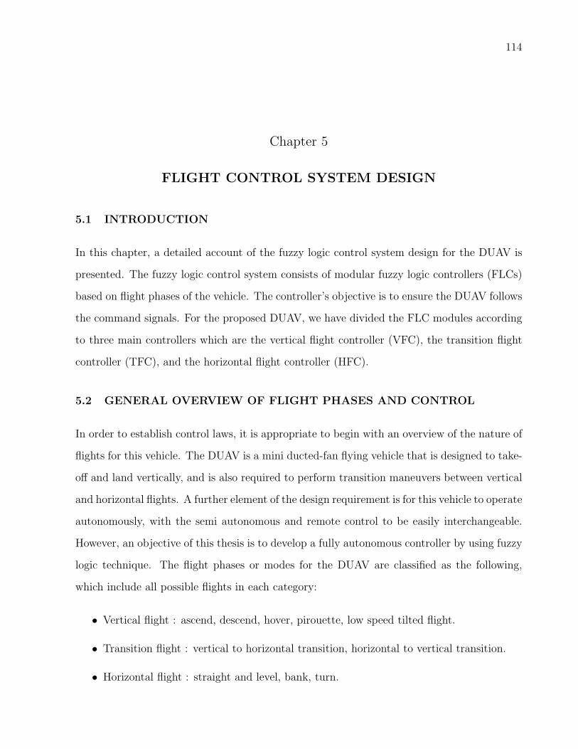
114

Chapter 5

FLIGHT CONTROL SYSTEM DESIGN

5.1 INTRODUCTION

In this chapter, a detailed account of the fuzzy logic control system design for the DUAV is

presented. The fuzzy logic control system consists of modular fuzzy logic controllers (FLCs)

based on flight phases of the vehicle. The controller’s objective is to ensure the DUAV follows

the command signals. For the proposed DUAV, we have divided the FLC modules according

to three main controllers which are the vertical flight controller (VFC), the transition flight

controller (TFC), and the horizontal flight controller (HFC).

5.2 GENERAL OVERVIEW OF FLIGHT PHASES AND CONTROL

In order to establish control laws, it is appropriate to begin with an overview of the nature of

flights for this vehicle. The DUAV is a mini ducted-fan flying vehicle that is designed to take-

off and land vertically, and is also required to perform transition maneuvers between vertical

and horizontal flights. A further element of the design requirement is for this vehicle to operate

autonomously, with the semi autonomous and remote control to be easily interchangeable.

However, an objective of this thesis is to develop a fully autonomous controller by using fuzzy

logic technique. The flight phases or modes for the DUAV are classified as the following,

which include all possible flights in each category:

• Vertical flight : ascend, descend, hover, pirouette, low speed tilted flight.

• Transition flight : vertical to horizontal transition, horizontal to vertical transition.

• Horizontal flight : straight and level, bank, turn.

115

In a full mission, the DUAV maybe flying in all flight phases according to a pre-

defined flight trajectory. A snapshot of a DUAV mission trajectory is shown in Figure 5.1

which demonstrates the vehicle motion in a three-dimensional space. Table 5.1 summarizes

all flight phases depicted in this figure.

1

2

3

4

5

6

7

8

910

1112

13

Figure 5.1: A mission trajectory in 3D space.

Suppose the vehicle starts taking-off at point 1 and is required to land at point 13

when the mission has completed. The location of point 1 can be thought as ground station.

At point 1, DUAV takes-off vertically (ascends) until it reaches a desired altitude, and stay in

hover at point 2. To reach point 3, the DUAV performs low-speed tilted flight (LSTF). Then

the vehicle ascends to gain velocity and performs vertical to horizontal transition maneuver

(VtoH) at point 3 and finishes at point 4. From point 4 to 5, the vehicle is flying at a high

speed straight and level forward flight (SLF). At point 5, the DUAV executes horizontal to

vertical transition flight (HtoV), and completes it by hovering at point 6.

116

Table 5.1: Flight modes for the DUAV.

Trajectory Flight Mode

1 ⇒ 2 Start + Ascend

2 ⇒ 3 LSTF(FB)

3 ⇒ 4 Ascend + VtoH

4 ⇒ 5 SLF

5 ⇒ 6 HtoV + Hover

6 ⇒ 7 Pirouette + Descend

7 ⇒ 8 Ascend + VtoH

9 ⇒ 10 Bank + Turn

11 ⇒ 12 HtoV + Hover

12 ⇒ 13 Descend + End

To prepare for a change in the direction of motion, the vehicle pirouettes at point 6, or

directs its belly pointing angle to the desired direction. Next, it descends until it reaches at

point 7. Between points 7 and 8, the DUAV is performing VtoH maneuver again, and once

completed, it continues flying to point 9 in the SLF mode. At point 9, the vehicle banks and

turns, and when it reaches point 10, it has completed two turning loops. From point 10 to

point 11, the DUAV is back in a high speed SLF, then performs HtoV at point 11 and ends

at point 12. The vehicle descend at point 12 and finally landed at point 13.

The control during vertical flight is through a combination of throttle, elevator, aileron,

and rudder control. Although throttle is the primary control, the control of elevator and

rudder are essential to maintain stability during vertical flight. The details of vehicle motions

in vertical flight are shown in Figure 5.2. During hover, the DUAV may change its pointing

direction by pirouetting using aileron. Suppose we need to move the vehicle a few meters

around its hovering point, the first step is to perform pirouette so that the new heading would

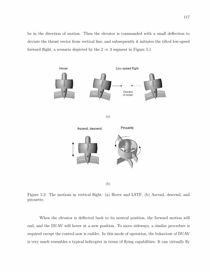
117

be in the direction of motion. Then the elevator is commanded with a small deflection to

deviate the thrust vector from vertical line, and subsequently it initiates the tilted low-speed

forward flight, a scenario depicted by the 2 ⇒ 3 segment in Figure 5.1

(a)

(b)

Figure 5.2: The motions in vertical flight: (a) Hover and LSTF, (b) Ascend, descend, andpirouette.

When the elevator is deflected back to its neutral position, the forward motion will

end, and the DUAV will hover at a new position. To move sideways, a similar procedure is

required except the control now is rudder. In this mode of operation, the behaviour of DUAV

is very much resembles a typical helicopter in terms of flying capabilities. It can virtually fly

118

to any direction in three-dimensional space: hover, heave, pirouette, forward and backward,

and sideways. The DUAV and helicopter also have the same principle of flights in this flying

mode. For instance, the principle of LSTF is similar to the helicopter motion in forward

flight where part of the thrust vector is made leaning towards the direction of motion. At this

moment, the only source of lift for DUAV is solely coming from the thrust since the dynamic

pressure is still low enough to enable wings to become effective.

If the pre-programmed flight is to directly arrive at high speed forward flight, it neither

needs to hover nor to fly in low-speed forward flight. All it has to do is to accelerate vertically

until it gains sufficient dynamic pressure at the propeller downstream, then the elevator is

deflected to perform the transition maneuver (3 ⇒ 4) to the high speed forward flight (4 ⇒

5). The vertical acceleration for the transition maneuver to horizontal flight can start from

a stationary position on the landing platform, or from hovering condition. This means the

DUAV has to be brought to rest or hover before it can perform this transition maneuver.

The VtoH flight is quite difficult to perform compared to the HtoV (reverse maneu-

ver). This is because the DUAV is unstable at low speed vertical flight prior to the maneuver,

whereas before the HtoV, the DUAV is already at a high speed stable flight. As we have dis-

cussed earlier, the vertical flight is the most unstable flight regime. The transition maneuvers

can be conducted by controlling both δe and δth. At any moment during the transition, eleva-

tor controls the required pitching moment, while thrust generates a specific forward motion.

Setting δth to constant until just before the maneuver completes is also a possible approach.

However, it is very important to note that once the vehicle body has rotated completely, the

DUAV must accelerate in order to gain sufficient dynamic pressure, and consequently, the

lifting surfaces are able to support the vehicle’s weight during horizontal flight.

Note that it is unsafe to perform the VtoH transition maneuver when the DUAV is

in LSTF. Increasing the excessive thrust at this orientation, may result in the uncontrolled

vehicle situation since the weight of the DUAV is still not supported by the lift of the wing.

This is because the tilted forward flight is still a thrust supported flight regime and the

119

dynamic pressure is ineffective at the moment. If the DUAV is performing LSTF, the DUAV

must be returned to hover first, then accelerates in curvature trajectory as described above

to complete the VtoH transition.

Suppose when the vehicle is flying in the SLF mode horizontally, then it is commanded

to hover again at point 6, possibly due to the mission requirement. To hover, it has to perform

a reverse HtoV maneuver as shown at 5 ⇒ 6 segment in Figure 5.1. The HtoV is less difficult

to implement since the DUAV is already in high speed before the maneuver. This means

at this high-speed forward flight, all control surfaces are fully effective (sufficient dynamic

pressure), so deflecting the elevator to perform a push-up maneuver is quite simple. As

the DUAV reaches the vertical attitude, the throttle can be reduced so the vehicle starts to

decelerate and finally stay in hover at point 6.

HtoV is a very quick maneuver that normally lasts between 2 to 4 s. During this

short period HtoV maneuver, the throttle can be set to constant at the appropriate stetting.

However, the HtoV flight is not just a matter of controlling only the throttle, but also involves

the control of other control surfaces similarly as required during the take-off. The vehicle may

descend to a lower altitude as shown at the 6 ⇒ 7 flight segment in Figure 5.1. Figure 5.3

shows the schematic of ascend, VtoH, SLF, HtoV, hover, and descend on the xz plane.

Back to Figure 5.1, suppose the vehicle has to fly in the SLF mode again to reach

point 10. From point 7, the DUAV has to perform another VtoH maneuver (7 ⇒ 8), before

it can enter the horizontal wing-borne flight at 8 ⇒ 9. Once the DUAV enters the high speed

forward flight region, it behaves and functions like a typical fixed-wing airplane. It is free

to fly longitudinally, directionally, or laterally. The flight patterns between points 9 to 10

demonstrate the lateral-directional motions of the vehicle. As indicated in the figure, the

vehicle performs two loops which involve bank and turn motions. The corresponding controls

in lateral-directional motions are rudder and aileron. Then, another straight and level flight

brings the vehicle at point 11.

120

Figure 5.3: Schematic of ascend, VtoH, SLF, HtoV, hover, and descend flights on the xzplane.

When the mission is completed, the vehicle needs to land on the ground station at point

13. The vehicle gradually decreases its flight speed and prepared to perform the second and

last HtoV maneuver at point 11, completes at point 12, and consequently descends towards

the ground station at point 13. Having discussed all the possible motions of the DUAV and

its control in general, now is the time to develop the fuzzy logic controller for each flying

mode. The remaining sections will discuss the general perspective to a detailed outline of all

steps involved in the design of controllers. We begin with the approach to the control system

design for DUAV.

5.3 CONTROL DESIGN APPROACH

The general structure of an automatic flight control system (AFCS) is given in Figure 5.4

[107]. In this study, the aim is to replace the pilot role, shown on the top left section in

the figure with an autonomous flight controller based on fuzzy logic. Fuzzy logic control is

an intelligence approach that is able to incorporate some aspects of human intelligence with

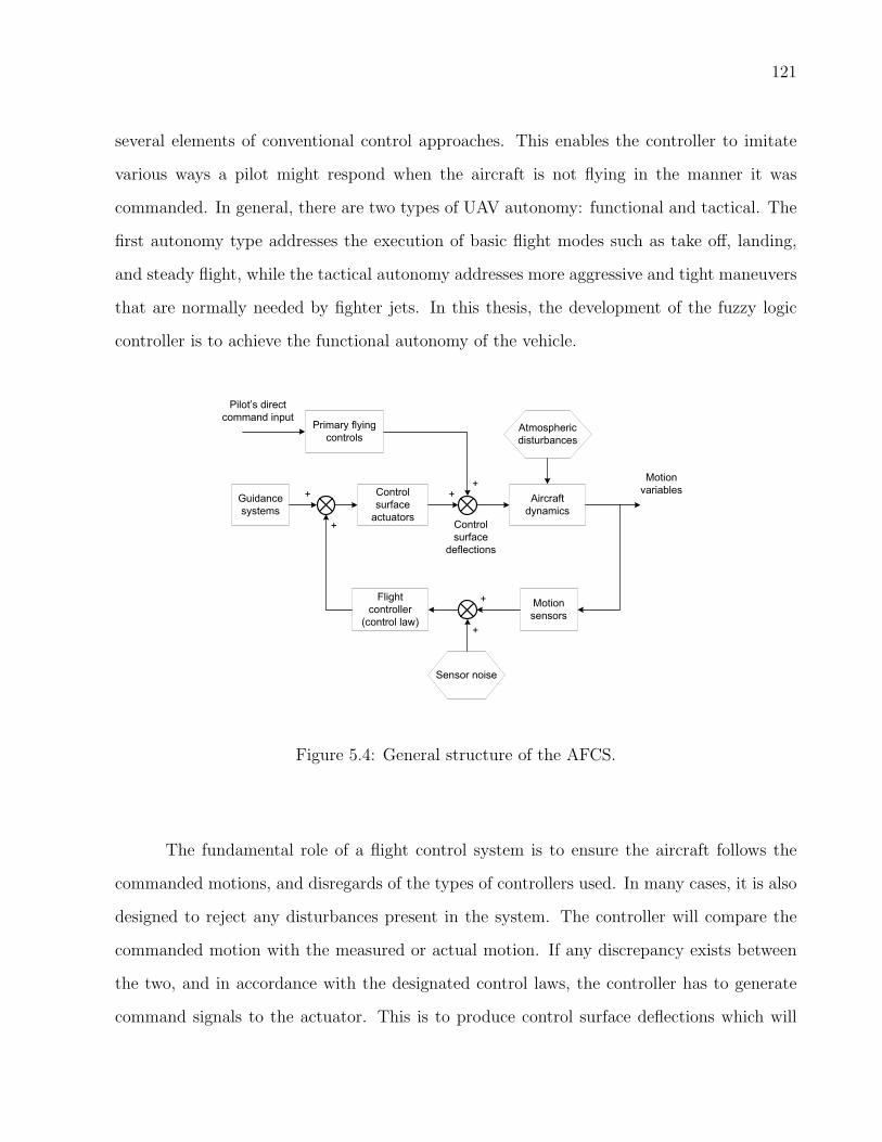
121

several elements of conventional control approaches. This enables the controller to imitate

various ways a pilot might respond when the aircraft is not flying in the manner it was

commanded. In general, there are two types of UAV autonomy: functional and tactical. The

first autonomy type addresses the execution of basic flight modes such as take off, landing,

and steady flight, while the tactical autonomy addresses more aggressive and tight maneuvers

that are normally needed by fighter jets. In this thesis, the development of the fuzzy logic

controller is to achieve the functional autonomy of the vehicle.

Guidance

systems

Control

surface

actuators

Aircraft

dynamics

Motion

sensors

Flight

controller

(control law)

Primary flying

controlsAtmospheric

disturbances

Sensor noise

Pilot’s direct

command input

Motion

variables

Control

surface

deflections

+

+

++

+

+

Figure 5.4: General structure of the AFCS.

The fundamental role of a flight control system is to ensure the aircraft follows the

commanded motions, and disregards of the types of controllers used. In many cases, it is also

designed to reject any disturbances present in the system. The controller will compare the

commanded motion with the measured or actual motion. If any discrepancy exists between

the two, and in accordance with the designated control laws, the controller has to generate

command signals to the actuator. This is to produce control surface deflections which will

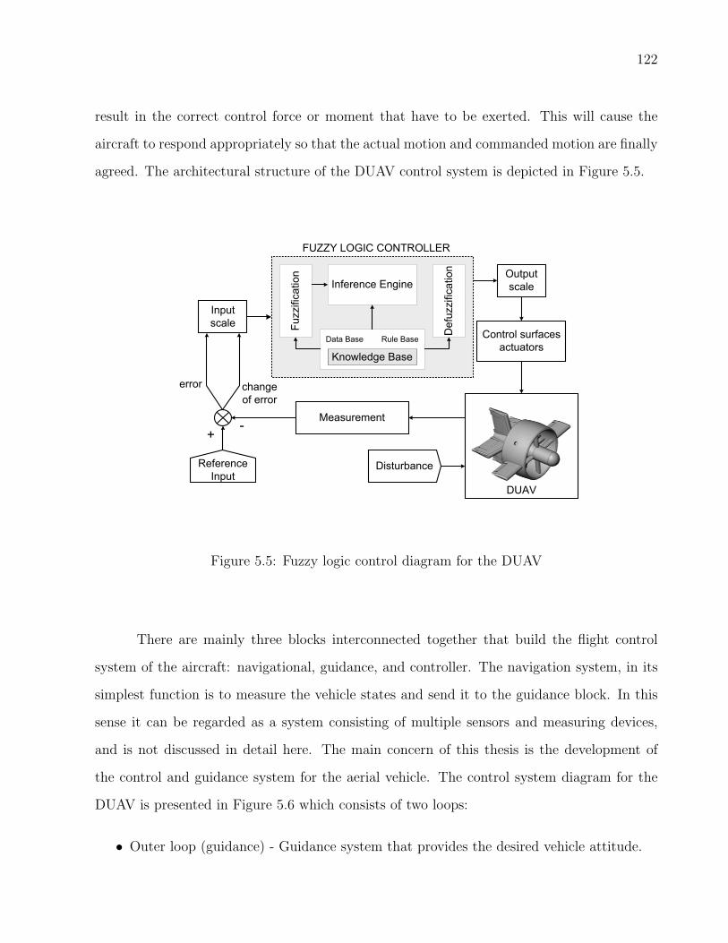
122

result in the correct control force or moment that have to be exerted. This will cause the

aircraft to respond appropriately so that the actual motion and commanded motion are finally

agreed. The architectural structure of the DUAV control system is depicted in Figure 5.5.

Fuzzification

Defuzzification

Inference Engine

Data Base Rule Base

Knowledge Base

Control surfaces

actuators

Measurement

Reference

Input

Output

scale

Input

scale

error change

of error

Disturbance

DUAV

FUZZY LOGIC CONTROLLER

+-

Figure 5.5: Fuzzy logic control diagram for the DUAV

There are mainly three blocks interconnected together that build the flight control

system of the aircraft: navigational, guidance, and controller. The navigation system, in its

simplest function is to measure the vehicle states and send it to the guidance block. In this

sense it can be regarded as a system consisting of multiple sensors and measuring devices,

and is not discussed in detail here. The main concern of this thesis is the development of

the control and guidance system for the aerial vehicle. The control system diagram for the

DUAV is presented in Figure 5.6 which consists of two loops:

• Outer loop (guidance) - Guidance system that provides the desired vehicle attitude.

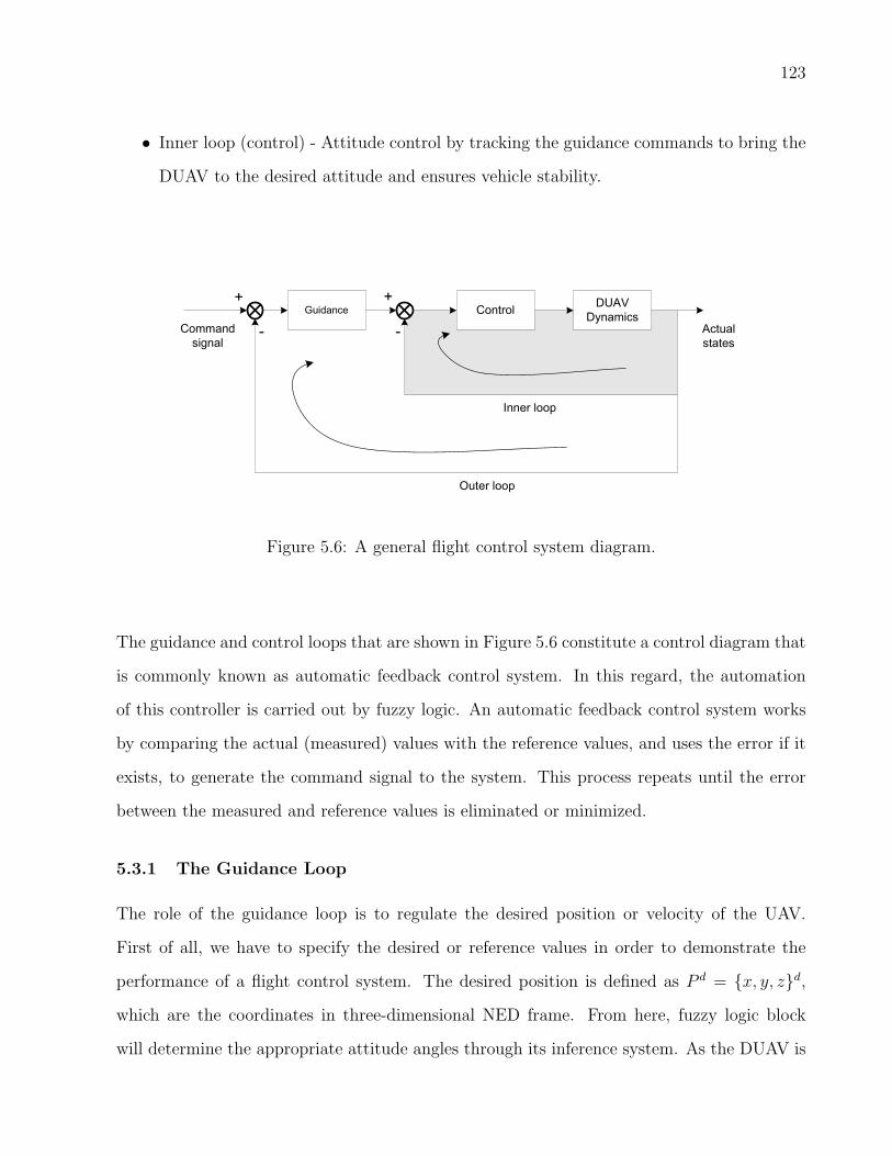
123

• Inner loop (control) - Attitude control by tracking the guidance commands to bring the

DUAV to the desired attitude and ensures vehicle stability.

Guidance ControlDUAV

Dynamics

Inner loop

Outer loop

Command

signal

Actual

states

+

-

+

-

Figure 5.6: A general flight control system diagram.

The guidance and control loops that are shown in Figure 5.6 constitute a control diagram that

is commonly known as automatic feedback control system. In this regard, the automation

of this controller is carried out by fuzzy logic. An automatic feedback control system works

by comparing the actual (measured) values with the reference values, and uses the error if it

exists, to generate the command signal to the system. This process repeats until the error

between the measured and reference values is eliminated or minimized.

5.3.1 The Guidance Loop

The role of the guidance loop is to regulate the desired position or velocity of the UAV.

First of all, we have to specify the desired or reference values in order to demonstrate the

performance of a flight control system. The desired position is defined as P d = x, y, zd,

which are the coordinates in three-dimensional NED frame. From here, fuzzy logic block

will determine the appropriate attitude angles through its inference system. As the DUAV is

124

flying towards the reference position, the commanded attitude angles are continue to change,

primarily based on the current vehicle speed and position error. For example, in the case of

LSTF flight towards north, as the DUAV draws nearer to the desired point, the commanded

θv is decreased. It is because the smaller θv causes the UAV to slow down, ready to hover at

the desired location.

In fuzzy logic flight guidance, the one to one solution of attitude angles for a given

trajectory error was not known until we put the controller to the test. This is due to the

nonlinearity and the fuzziness behaviour that presents in the algorithm. It is contrary to the

linear analytical method where for a given position error with some other known variables,

a unique solution for attitude angles can be obtained. In this guidance loop, the generation

of the desired attitude angles corresponding to the measured position error are bound by the

guidance laws.

5.3.2 The Control Loop

It is very important to have the DUAV flying at a specific attitude that eventually drives

the vehicle towards the reference position, and at the same time maintains the stability of

the flight. We use the commonly known Euler angles to represent the attitude of the DUAV.

Recall to the example that we have just discussed above, where from hover condition, the

DUAV tilts forward in order to initiate the motion to the north. The tilt angle, θv determines

the resulting translational speed of the DUAV. Basically, when the DUAV is tilting at a big θv,

it dictates big thrust vector is diverts from the vertical line, and results in a higher forward

translational speed. However, if the θv is too big, it would be very hard to maintain the

stability of the flight, and also very hard to have sufficient thrust that maintains the vehicle’s

altitude.

The commanded tilt angle is determined from the guidance loop. The fuzzy block

in the control loop will take the commanded attitude angle as the input, and outputs the

appropriate elevator deflection. When the elevator is deflected at this angle, the vehicle

125

dynamics produces corresponding force and moment that finally brings the DUAV to that

commanded attitude angle. Since it is a feedback control loop, as long as the error between

reference and actual θv exists, the fuzzy system will also generate the corresponding signal

to rectify the error. In this example, the general requirement for the DUAV to fly at nearly

constant altitude, maintain stability, and fly at an acceptable speed is achieved through the

combination control of the elevator and throttle. Essentially, the control laws will guide the

purpose of the respective control surface deflection for any given commanded attitude angle.

In general, the control loop consists of modular FLCs that are assigned to control flight

variables via corresponding control surfaces as follows:

• Throttle to control the altitude rate, h

• Elevator to control the vertical pitch , θv

• Differential elevator to control vertical roll, φv

• Rudder to control the vertical yaw, ψv

The designation of these FLCs in the control loop can also be seen in Figure 5.7. It is a

feedback control loop consisting four fuzzy logic controllers that control the DUAV motion.

5.3.3 Control Design Steps

The first step in fuzzy logic control system design is to have the knowledge on the considered

physical system. This knowledge can be acquired either from experts or from examining the

dynamics model of the system. For DUAV, the knowledge from experts is not yet available,

therefore at this stage we still can gain basic knowledge of its behaviour through simulation.

To implement this, we develop the mathematical model of the DUAV using nonlinear equa-

tions described in Chapter 4. Next we run a series of computer simulation of the vehicle

using MATLAB R© and Simulink R© platform. This simulation was carried out repetitively with

careful consideration in order to study the vehicle behaviour in various flight conditions, and

126

Elevator

Rudder

Throttle

Aileron

FLCs

DUAV

Command

signalActual

signal+

thδ

eδ

rδ

aδ

Sensors

Figure 5.7: The control loop consists of four control surfaces.

also to learn how it would respond to control inputs. The design steps of building a FLC are

depicted in Figure 5.8.

In the first design step, we need to define the control objective. In this thesis, the

objective of the control system design is to have the functional autonomy of the DUAV. The

functional autonomy addresses the execution of basic flights of the vehicle which are included

in three phases of flights : vertical, transition, and horizontal flights. The autonomous func-

tionality of all flight types will be discussed in detail in a later section of this chapter. When

the control objectives have been clearly defined, we can move to the next step of the design

processes which is to design the fuzzy controller by using membership functions and rule-

based concepts. This involves choosing the appropriate fuzzy variables, determining fuzzy

sets and membership functions to represent the interested variables, and develop appropriate

fuzzy rules. Detailed material on all these fuzzy parameters is available in Chapter 2.

The third step of the fuzzy controller design as depicted in the third block in Figure

5.8 is to tune the controller by altering several fuzzy parameters. This task was discussed in

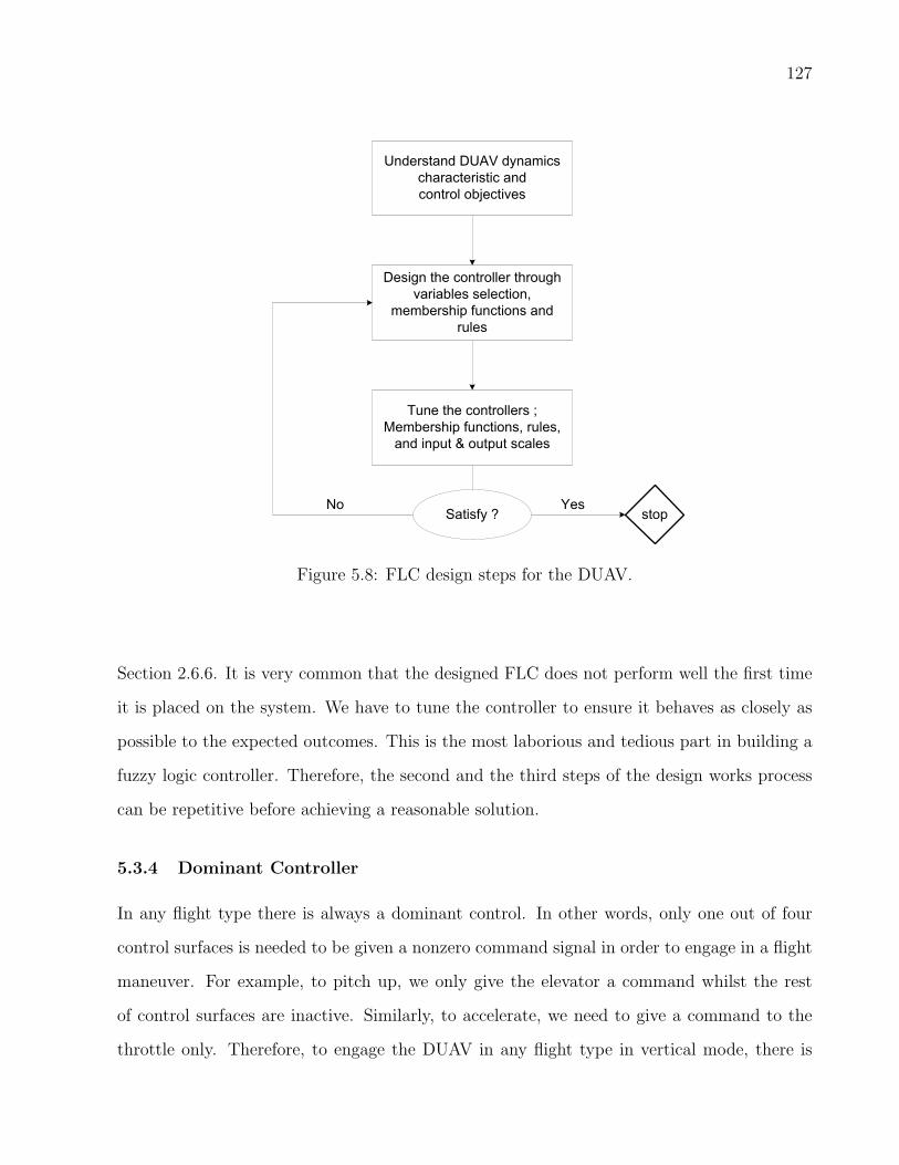
127

Understand DUAV dynamics

characteristic and

control objectives

Design the controller through

variables selection,

membership functions and

rules

Tune the controllers ;

Membership functions, rules,

and input & output scales

stopSatisfy ?YesNo

Figure 5.8: FLC design steps for the DUAV.

Section 2.6.6. It is very common that the designed FLC does not perform well the first time

it is placed on the system. We have to tune the controller to ensure it behaves as closely as

possible to the expected outcomes. This is the most laborious and tedious part in building a

fuzzy logic controller. Therefore, the second and the third steps of the design works process

can be repetitive before achieving a reasonable solution.

5.3.4 Dominant Controller

In any flight type there is always a dominant control. In other words, only one out of four

control surfaces is needed to be given a nonzero command signal in order to engage in a flight

maneuver. For example, to pitch up, we only give the elevator a command whilst the rest

of control surfaces are inactive. Similarly, to accelerate, we need to give a command to the

throttle only. Therefore, to engage the DUAV in any flight type in vertical mode, there is

128

always a dominant control surface that can initiate the vehicle into that desired flight motion.

Table 5.2 shows the corresponding dominant controls for all flight modes. For example, the

dominant controller in ADH (ascend, descend, hover) is the throttle setting δth.

Table 5.2: The concept of dominant control.

Flight Mode Dominant Control

ADH δth

Vertical Pirouette δa

Flight LSTF(FB) δe

LSTF(LR) δe

Transition VtoH δe

Flight HtoV δe

Straight δth

Horizontal Climb δe

Flight Bank δa

Turn δr

The table is not to indicate that in a particular flight, the controller needs to give

command on the dominant control surface only. Rather, the FLCs control all the control

surfaces simultaneously in any given flight. However, our approach is for any given flight

mode, we concentrate more on the corresponding dominant control surface to ensure the

control objectives set fourth in that particular flight are achieved, with the assumption that

less effort is needed by non-dominant control surfaces to correct attitude errors. For example,

consider an ascending flight that is required to reach a hover altitude, and must complete

this flight within a specified time. The DUAV is also required to ascend in a perfect vertical

axis. Assume this flight takes place in less windy surroundings.

Because good vehicle attitude and stability was maintained throughout, during the

129

climbing it follows an almost perfect vertical axis. However, it was found that the vehicle’s

speed was too low. Therefore, we have to put more effort to tune the throttle controller

until it reaches at the appropriate settings so as to cause the vehicle to move faster. Also

somewhere during the flight, the DUAV was tilted with a very small negative θv due to weak

wind gust. In response to this tilt angle, minimal control effort was given to the elevator

controller to rectify this attitude error. In this case, the main (dominant) controller is the

throttle, while elevator becomes less important. In Section 5.4.1, we will discuss the use of

dominant controller in the vertical flight guidance.

5.3.5 Synthesis of Fuzzy Rules

The essence of a FLC is the generated rules are heuristic in nature, and reflect the experience

of an expert who can remotely control the vehicle. In the case of computer simulation, to

develop fuzzy rules we need to have a mathematical model that clearly shows the relationship

between the control vector and the system variables. To appreciate this relationship, we will

expand the six degrees of freedom equations of motion derived in the previous chapter until

the control variables appeared in it. The nonlinear forces and moments in Equations 4.11 to

4.16 can be rearranged in the form of velocity and body rates as follows:

u = rv − qw + gx + ax (5.1)

v = −ru+ pw + gy + ay (5.2)

w = qu− pv + gz + az (5.3)

p =1

IxIz − I2xz

Ixz[Ix − Iy + Iz]pq − [Iz(Iz − Iy) + I2xz]qr + Izl + IxzN (5.4)

q =1

Iy(Iz − Ix)pr − Ixz(p

2 − r2) +M (5.5)

r =1

IxIz − I2xz

[(Ix − Iy)Ix + I2xz]pq − Ixz[Ix − Iy + Iz]qr + Ixzl + IxN (5.6)

The acceleration terms in Equations 5.1 to 5.3 can be written as:

ax = (1/Mass)(Fxa + Fxp) (5.7)

130

ay = (1/Mass)(Fya + Fyp) (5.8)

az = (1/Mass)(Fza + Fzp) (5.9)

Expand all force expressions in 5.7, 5.8, and 5.9 with its build-up components, and all other

inclusion variables, coefficients, and terms, and then substitute these expanded forces expres-

sions back in Equations 5.1, 5.2, and 5.3. Also, expand all body rates and velocities terms in

Equations 5.1, 5.2, and 5.3, finally yields,

u = −qw + rv + gSinθ +1

m[CosαCobβqS(Cd +

(CL − CLo)2

πeAR+ CDδe

δe

+CDδaδa+ CDδr

δr)− CobαSinβqS(CYββ + CYαα+ CYδr

δr

+b

2VT(CYpp+ CYrr))− SinαqS(CLo + CLαα+ CLδe

δe

+c

2VT(CLα

α+ CLqq))] +4

π4ρR4Ω2CT (5.10)

v = −ru+ pw + gy +1

m[−CobαSinβqS(Cd +

(CL − CLo)2

πeAR+ CDδe

δe

+CDδaδa+ CDδr

δr) + CobβqS(CYββ + CYαα+ CYδr

δr

+b

2VT(CYpp+ CYrr))− SinαSinβqS(CLo + CLαα+ CLδe

δe

+c

2VT(CLα

α+ CLqq))] + Fyfan (5.11)

w = −pv + qu+ gCobθ +1

m[−SinαqS(Cd +

(CL − CLo)2

πeAR+ CDδe

δe

+CDδaδa+ CDδr

δr)− CobαqS(CLo + CLαα+ CLδeδe

+c

2VT(CLα

α+ CLqq))] + Fzfan (5.12)

Similarly, expand all inertia and body rates expressions in Equations 5.4, 5.5, and 5.6 with

all the inclusion coefficients and variables, we have the fully expanded expressions of body

angular acceleration as follows,

p =1

IxIz − I2xz

Ixz(Ix − Iy + Iz)pq − (Iz(Iz − Iy) + I2xz)qr + Iz(

1

2ρV 2

T Sb(Clββ

+Clδaδa+ Clδr

δr +b

2VT(Clpp+ Clrr))) + Ixz(

1

2ρV 2

T Sb(CNββ + CNδa

δa

131

+CNδrδr +

b

2VT(CNpp+ CNrr))) (5.13)

q =1

Iy(Iz − Ix)pr − Ixz(p

2 − r2) +1

2ρV 2

T Sc(CMo + CMαα+ CMδeδe

+c

2VT(CMα

α+ CMqq)) (5.14)

r =1

IxIz − I2xz

((Ix − Iy)Ix + I2xz)pq − Ixz(Ix − Iy + Iz)qr + Ixz(

1

2ρV 2

T Sb(Clββ

+Clδaδa+ Clδr

δr +b

2VT(Clpp+ Clrr))) + Ix(

1

2ρV 2

T Sb(CNββ + CNδa

δa

+CNδrδr +

b

2VT(CNpp+ CNrr))) (5.15)

What we have just expanded in Equations 5.10 to 5.15 are all nonlinear forces and moments

equations in body-axis that show relationships between the state variables and control sur-

faces. Clearly from these equations, the nature of variables involved are highly coupled and

nonlinear. The one to one relationship between any variables is impossible to determine, and

the only means to solve this nonlinear problem is through numerical analysis. However, the

idea of expanding all these forces and moments equations is to have at least some kind of

appreciation on how the control surfaces drive the system.

Fortunately, when we use fuzzy logic as a mean to control the DUAV, this nonlinearity

that presents in the system is no longer of interest. The fact is that the development of the

fuzzy logic controller is independent on decoupling the system [115]. In other words, it is not

important to understand thoroughly how the nonlinearity behaves within the system, as long

as the system responds appropriately upon any given inputs. This is one of the advantages of

fuzzy logic where it can encompass the nonlinearities in the system. The fuzzy logic controller

may be designed based on two different methods [116, 47] as follows:

1. Design the controller based on the knowledge available from experts.

2. Develop the model of the plant from measurement, and first principle. Use this model

to design the controller or incorporate this model in a model-based control scheme.

132

The first method is out of the question because the actual vehicle is not built yet.

Therefore, we adopt the second method where the FLC are designed based on the knowledge

acquired through examining the vehicle characteristic and its response to control surface

inputs. We can achieve this by running a series of flight simulations that include all flight

phases. Behind this simulation program are dynamical relationships dictated in Equations

5.10 to 5.15 above. In this way, we gather a comprehensive “expert” knowledge of the problem

at hand. We will discuss the flight simulation details in the next chapter.

We have defined the FLC should acquire the generic skills of the pilot. It can be

thought that the DUAV is operated by a skilled pilot, which in this case his or her jobs is

replaced by the FLC. Hence, we can expect the FLC will do what a pilot would normally does

in controlling the vehicle. By having the knowledge of the vehicle characteristic and response

towards the control inputs, we can derive the appropriate fuzzy rules that eventually formed

an automatic flight control system for the DUAV. The approach to develop the fuzzy rules

is based on the method described in [117]. It is a very different approach compared to

the conventional techniques in developing a flight controller. The method used total energy

concepts in order to develop multi-input-multi-output (MIMO) flight controllers.

In this approach, airspeed and altitude of the aircraft are both controlled by elevator

and thrust, while heading and sideslip are both controlled by ailerons and rudder. Certainly,

these control concepts have much correspondence with pilot’s heuristics in controlling the

aircraft. The total energy concept was used to develop fuzzy rules for both longitudinal and

lateral-directional controls. In longitudinal flight, consider the kinetic energy which related

to vehicle’s velocity, and the potential energy linked to vehicle’s altitude. In this context,

thrust increases the total energy, while an exchange between kinetic and potential energy is

achieved by changes in the pitch angle. This fact can be examined through the following

cases. If the DUAV flies too low and too slow, the controller will increase the thrust in order

to increase the energy of the vehicle. On the other hand, if the vehicle flies too low but the

velocity is too high, the controller has to increase the pitch angle through elevator deflection.

133

These are examples of typical control problems in straight and level flight

Based on this principle, rules are derived. Here, fuzzy rules are generated in linguistic

rather than in mathematical terms. When we derive fuzzy rules, we are actually establishing

a guideline on how the FLC can make control decision on numerous flight problems. Back to

the first case described above, the problem might be written as:

If the current altitude is around x m, and the current velocity is y m/s below the

desired cruise speed, what would the throttle setting be?

The choices of adjusting the throttle setting in this case would be: increase substantially,

increase slightly, no change, decrease slightly, and decrease substantially. Based on the knowl-

edge about the system that we have, a rule can be derived as follows:

IF altitude error is X, AND velocity error is Y, THEN throttle setting is Z

where X, Y, and Z are fuzzy sets representing altitude error, velocity error, and throttle setting

respectively. A similar procedure can be applied for the lateral-directional flight control

problem. Normally, the pilot uses the roll angle command to control the heading angle and

lateral deviation, while sideslip is controlled by rudder deflection. In the development of the

FLC for lateral motion, an example of fuzzy rule that can be derived is:

IF roll angle error is X, AND rate of roll angle error is Y, THEN aileron deflection is Z

where in this example, fuzzy sets for roll angle error, rate of roll angle error, and aileron

deflection are represented by X, Y, and Z respectively. A complete set of rule base that was

developed in this thesis will be discussed further in greater detail in their respective flight

phases discussion later. The derived fuzzy rules can be thought as the guidance or control

laws, depending in which part these rules are applied.

The tasks of controlling the aircraft that we have just discussed are quite common

for a skilled pilot. However, the challenge here is how we can design fuzzy rules that can

134

function effectively in the same manner as a pilot does, or perhaps even better. The ability

of FLCs to reason, and to decide on every flight problem leads to the possession of intelligent

characteristic in controlling the flights. In what follows, we discuss the specification of the

fuzzy logic properties and variables used in this thesis.

5.3.6 Properties of the FLC

As the autonomous flight of the DUAV involves several flight phases, it is very convenient

to divide the controllers into a number of modules according to these flight phases. There

are several properties of fuzzy logic that are common to all FLC modules, and also some

fuzzy properties that are different between one FLC module to another. The common fuzzy

logic properties in all FLCs are the number of input variables, membership functions, fuzzy

sets, and number of rules, while fuzzy properties that are differ between FLCs are the chosen

input and output variables, fuzzy rules and scaling factors. In this section, we discuss the

specification of the fuzzy logic controllers.

5.3.6.1 Input and Output Variables

The most important step in building a fuzzy logic controller is to specify the problem, which

is to determine the input and output variables. In determining the type of input variables, we

adopt a technique that was proven to have given a good performance in many applications

[75], which is the use of error and rate of error for input variables. In all FLC modules,

the use of error and rate of error for input variables is consistent. But of course on each

flight problem, the chosen input and output variables are different from one to another. For

example, it is readily apparent that the output variable for pitch controller is elevator, while

for yaw controller is rudder.

Each FLC consists of 2 input variables and 1 output variable. The process of choosing

appropriate input and output variables for FLC modules is an important element in the

FLC design. A detailed treatment on this matter is included in each FLC module that we

135

will develop later. Fuzzy logic controller is also sometimes referred as PD-type or PI-type,

a classification based on the type of the output variable [51]. A PD-type fuzzy controller

generates an output signal from error and rate of error of input variables, whilst a PI-type

fuzzy controller generates an increment of output signal from the same form of input variables

as in PD-type. Therefore, in this thesis, most of the FLCs are of 2-input 1-output PD-type,

except for the throttle controller in vertical flight where the output is either an increment or

decrement to the current throttle setting (PI-type).

5.3.6.2 Fuzzy Sets, and Membership Functions

Having input and output variables determined, the next step is to choose fuzzy sets to rep-

resent all these linguistic variables. Fuzzy sets can have a variety of shapes that are charac-

terized by membership functions. The triangular shape of fuzzy sets is the most often used

by the designer, and usually provides an adequate representation of the expert knowledge

[66]. We choose five fuzzy sets which are negative-big (NB), negative-small (NS), near-zero

(NZ), positive-small (PS), and positive-big (PB). These fuzzy sets are represented by trian-

gular membership functions as shown in Table 5.3. Both input and output variables have the

same fuzzy sets. That is, each of the input or output variable has five fuzzy sets that are

characterized by five triangular membership functions correspondingly.

Each membership function is defined by three points on the universe of discourse. Five

triangular membership functions present a symmetrical arrangement with the central mem-

bership function (NZ) having its apex at zero on the universe of discourse. For NB and PB

fuzzy sets, their membership functions are disconnected at their apex. Note that the base

point of any membership function is coincident with the base of another membership func-

tion. This ensures all membership functions are linked together. By arranging membership

functions in this way, it makes the value of any input variable is consistently a member of two

fuzzy sets. In Figure 5.3, it can also be noted that when a variable of any set has a degree of

membership of unity, it is not a member of another sets.

136

Table 5.3: Fuzzy sets and membership function.

-1 -0.75 -0.5 -0.25 0 0.25 0.5 0.75 10

0.2

0.4

0.6

0.8

1

Universe of discourse, X

Degre

e o

f m

em

bers

hip

, µ

A(X

)

NB NS NZ PS PB

The fuzzy sets:

NB: Triangular (-1,-1,0.5)

NS: Triangular (-1,-0.5,0)

NZ: Triangular (-0.5,0,0.5)

PS: Triangular (0,0.5,1)

PB: Triangular (0.5,1,1)

5.3.6.3 Universe of Discourse, and Scaling Factors

The universe of discourse for all membership functions are normalized in the range of [-1 1].

This is done by dividing the base numerical values with input and output scales. In Figure

5.5, the input and output scales are depicted in the top left and top right blocks respectively.

The purpose of scaling factors is to maintain signals between inputs and outputs are within

the limit for which fuzzy rules are defined [47].

Scaling factors give effect to the controller’s performance in terms of response over-

shoot, rise time, and settling time. There is no formal approach to tune scaling factors for

137

FLC. Scaling factors on each FLC may differ, and after running several simulation loops, it

was found that scaling factors in the range of 0.01 to 7 have resulted in a reasonable solution.

The scaling factors for each FLC are provided in their corresponding section in Chapter 6.

5.3.6.4 The Rules

At this point, we have seen in Section 2.6.4 how linguistic expressions are transformed into

linguistic rules, and their purpose for fuzzy rules. Fuzzy rules can be thought as control

laws, a standard term used in relation to flight control systems. These rules are used by the

controller to react against various types of system responses such as overshoot, undershoot,

steady-state error, and transient condition. These possible responses should be controlled in

order to drive the vehicle to the desired states or at least close to it.

Whilst it is desirable to a have a controller with fewer rules, care must be given to

preserve important relationships between state variables [68]. A good balance between a

small number of rules and accurate representation of the coupling in the system is needed to

achieve an efficient and effective controller. Since we have decided to have five fuzzy sets on

each input variables, the maximum rules is 5 × 5 = 25 rules. Therefore, a set of 25 rules base

is maintained in each FLC.

5.3.7 Computational Tools

Now we have defined all fuzzy logic parameters that are needed to build a fuzzy logic con-

troller. The next task is to encode these parameters into a suitable computational tool. In

this study, we use MATLAB R© Fuzzy Logic Toolbox which provides a systematic framework

for computing fuzzy rules together with the graphical user interfaces (GUI). A snapshot of the

GUI for this toolbox is shown in Figure 5.9. Once the process of encoding fuzzy parameters

on the Fuzzy Logic Toolbox tool is completed, the fuzzy logic controller is now ready for use.

138

FLC Editor Control Surface ViewerMembership Function Editor

Rules Editor Rules Viewer MATLAB Command Window

Figure 5.9: A snapshot of Fuzzy Logic Toolbox GUI.

5.4 VERTICAL FLIGHT CONTROLLER

The control of vertical flight is the most challenging task as in this flight condition the

vehicle is very unstable, and the mode of operation is the most novel in comparison to

that of a conventional aircraft. Instability in this flight mode is considerable due to the

low dynamic pressure that causes the wing and tail to ineffectively provide any force or

moment. Therefore, vertical flight control for the DUAV is achieved only through the fan

thrust and force and moment due to fan slipstream over the cruciform control surfaces. For

convenience in designing numerous FLCs, the associated motions of the vehicle in vertical

flight are categorized as:

• Ascend, descend, hover

• Pirouette

• Low-speed tilted flights

The vehicle ascends for take-off or to hover at higher altitude, and adversely descends

to land or to hover at lower altitude. It also performs vertical spin or pirouette, which is

139

normally required if it has to change the vertical heading, or conveniently referred to as

vehicle belly pointing angle. Pirouette can also be considered as a normal yaw motion during

hover. In a typical mission, the vehicle may need to change its hovering position. This can be

achieved by performing low-speed tilted flight (LSTF) to the desired location, which is done

by tilting the vehicle towards the direction of motion. The DUAV can fly in LSTF mode

to virtually any direction horizontally either through forward-backward or sideways motions.

All these motions are depicted in Figure 5.2.

The free body diagrams of the DUAV in vertical flight are shown in Figure 5.10, that

includes front, side, and top views, with the vehicle’s belly is on the right side of Figure 5.10(a).

The figure shows all forces, moments, and all other variables that are easily recognized from

their notations used. Note that all quantities shown in Figure 5.10 are in their positive sense.

The full set of nonlinear equations of motion derived in Chapter 4 can also be derived in a

similar manner based on these free body diagrams.

As clearly defined earlier, the development of FLCs in this thesis is based on the full

six degrees of freedom nonlinear model of the vehicle. Evidently, when using a nonlinear

vehicle model, the nonlinear interaction between control inputs exists. A quick look into this

phenomenon can be observed when an input is given to the aileron, it causes the aircraft not

only to roll, but to turn as well. However, fuzzy logic has proven to be a successful control

approach for complex nonlinear systems [118, 119].

In vertical flight, the desired flying characteristic and stability can be achieved by

assigning the controller to control the velocity components of w, v, h, and also roll rate

p. The corresponding control surfaces for these velocities and angular rates are elevators,

rudders, engine throttle, and ailerons respectively. The vertical flight is best performed at a

low translational velocity as the aerodynamic forces and moments due to the translational

motion of the vehicle are negligible. Therefore, in this flight regime, the only force and

moment that significantly effect the vehicle motion are gravitational and propulsive [25]. The

ineffective aerodynamic of the wing due to low dynamic pressure during a relatively low speed

140

(a) Side view (b) Front view

mg

φp,

Fy, v

Fz, w

Laδ

aδ

Y

Z

(c) Top view

Figure 5.10: The free body diagram in vertical flight.

vertical flight contributes to the instability to the vehicle.

Whilst the throttle controls the axial velocity, the DUAV also has to be stabilized in

vertical flight by using control surfaces. Lift and drag components generated from the control

surfaces are responsible for trimming the unwanted moment during vertical motion. Here it is

evident that the stability of vertical flight is very much dependent on how well the controller

commands the elevator and rudder. By using feedback control system, FLCs receives the

141

error and rate of error signals that were calculated from the difference between set points and

current vehicle states. From these errors, FLCs drive the system to the desired states.

5.4.1 Vertical Flight Guidance

The role of vertical flight guidance system is to estimate appropriate command signals for

vertical Euler angles (φvc , θvc , ψvc) and altitude (hc) that are required by the control loop.

Upon receiving these signals, the control loop will command the control surfaces to deflect

accordingly in order to bring the DUAV to the desired position and attitude. The position

of the vehicle is defined in the three-dimensional NED frame which consist of north, east,

and height position coordinates [PN,PE, h], and a pointing angle, φv. The guidance loop

starts by comparing the current vehicle position with its reference position, and from here the

position error is obtained. Figure 5.11 shows a schematic of vertical flight guidance system.

Calculate the position error

and rate of position error ;

EPN = PNc – PN, d/dt (EPN)

EPE = PEc – PE, d/dt (EPE)

Desired hover

altitude

Desired belly

pointing angle

Current position

( PN, PE )

Desired position

( PNc, PEc )

cvθ

cvψ

cvφ

hc

PNE ,EPN

.

PEE ,EPE

.

PNvGVF

θ

PE

vGVF

ψ

Figure 5.11: The vertical flight guidance system.

Two position errors in north and east (EPN , EPE), together with its rates (EPN ,

EPE) are used as inputs to two FLCs in guidance system, GVFPNθvand GVFPEψv

respectively.

142

Apparently, commanded signals for the desired hover altitude, hc and the desired belly point-

ing angle, φvc can be given directly because of their independence from other variables. Af-

terward, all of four outputs from the guidance loop which are θvc , ψvc , φvc , and hc will be used

as inputs in the control loop. We use the acronym GVF (G:guidance, V:vertical, F:flight) to

represent FLC for vertical flight guidance. Superscript notation on each FLC refers to its

fuzzy input, while subscript notation represents its output.

Table 5.4 shows a complete list of FLCs used in the vertical flight guidance and control.

As indicated in the flight guidance row in the table, GVFPNθvand GVFPEψv

are used to guide

all flight modes in vertical flights. Table 5.4 also provides important information on the

functionality of each FLC in various flight modes. To understand this, take a look at the

initial and command values section in the table. Here we have five variables that are needed

to demonstrate all flight modes in vertical flight. Consider the setting of these five variables

for the ascend flight. From an initial rest condition (hinit = h1 m), the DUAV is commanded

to perform ascending flight, and is required to hover at the altitude of h1 m. To ensure a

perfect ascend, the rest three command signals, PNc, PEc, and φvc are all set to zero.

Throttle ensures sufficient thrust is provided during lift off from the ground. At the

same time, elevator, rudder and aileron have the task of stabilizing the vehicle by maintaining

the vehicle orientation in vertical attitude throughout the flight. By setting command signals

of PNc, PEc, and φvc equal to zero, this depicts an important element that the corresponding

controllers have to function. It means at any moment during the ascending flight, if the

position of the vehicle deviates towards the north or south, or encounters heading error, the

corresponding controller will compensate these errors by bringing the vehicle to the reference

PNc, PEc, and φvc .

In case where disturbances are too weak to cause position errors during ascend, all

these three controllers: elevator, rudder, and aileron are in an inactive state. Hence, the only

active and dominant control in ascending flight is the throttle. This case gives a meaning

to the dominant control concept that was discussed in Section 5.3.4. The function of FLCs

143

in the rest of four flight modes depicted in Table 5.4 can be grasped in a similar manner.

Apparently, pirouette and both LSTFs should take place at a constant altitude. The same

altitude settings for both hinit and hc in all these three flight modes confirmed these flights

are programmed to happen at the same altitude.

Table 5.4: Guidance and Control FLCs in vertical flight, and initial and target settings.

Flight Mode Ascend Descend Pirouette LSTF(FB) LSTF(LR)

Elevator GVFPNθvGVFPNθv

GVFPNθvGVFPNθv

GVFPNθv

Flight Rudder GVFPEψvGVFPEψv

GVFPEψvGVFPEψv

GVFPEψv

Guidance Aileron Desired belly pointing angle, φvc

Throttle Desired hover altitude, hc

Elevator CVFθvδe

CVFθvδe

CVFθvδe

CVFθvδe

CVFθvδe

Flight Rudder CVFψv

δrCVFψv

δrCVFψv

δrCVFψv

δrCVFψv

δr

Control Aileron CVFφv

δaCVFφv

δaCVFφv

δaCVFφv

δaCVFφv

δa

Throttle CVFhδth CVFhδth CVFhδth CVFhδth CVFhδth

hinit h1m h1m h1m h1m h1m

Initial and hc h2m h2m h1m h1m h1m

Command PNc 0 0 0 x1m 0

Values PEc 0 0 0 0m y1m

φvc 0 0 φvc10 0

Table 5.5 summarizes the inputs and outputs variables for all FLCs used in vertical

flight guidance and control loops.

5.4.1.1 Low-Speed Tilted Flight Guidance

The vehicle can translate at low speeds in vertical attitude by tilting the thrust vector [3]

into the direction of motion. We defined this type of flight as low-speed tilted flight (LSTF),

144

Table 5.5: Input and output variables for FLCs in VFC.

Fuzzy Variables Input Output

GVFPNθvEPN, EPN θvc

GVFPEψvEPE, EPE ψvc

FLC CVFθvδe

θvc , Eθvc δe

CVFψv

δrψvc , Eψvc δr

CVFφv

δaφvc , Eφvc δa

CVFhδth Eh, Eh δth

and it can be classified into two types based on the direction of motions: forward-backward,

and sideways (left-right). We first discuss the flight in forward-backward (FB) directions,

noted as LSTF(FB). Consider the DUAV hovers at the altitude of 60 m with zero pointing

angle (facing north), and is required to fly 100 m in north direction. Based on the guidance

laws, the FLC will reason at what θv that will bring the vehicle to the desired position. Also,

this tilted flight must take place in an acceptable range of flight speed, and simultaneously

maintains altitude and stability. The corresponding FLC that determine the commanded θvc

for a given PN input is GVFPNθv.

The input and output variables for GVFPNθvare EPN and EPN , and θvc respectively.

In previous sections, we have already discussed and justified the selection of fuzzy sets, type of

membership functions, and the number of rules that should be used in the development of the

FLC in this thesis. Five fuzzy sets are used: NB, NS, NZ, PS, and PB, and for membership

functions, we use the triangular type. Also, from the number of fuzzy sets that represent

input and output variables, we have also discussed that the number of rules should be 25.

Therefore, the task now is to develop these rules.

Back to the above example where the DUAV needs to change its hovering position 100

145

m to the north. The error, E and rate of error, E are calculated as:

E = Desired value− Actual value (5.16)

E = d/dt(E) (5.17)

Hence, the north position error, EPN and its rate, EPN are calculated as:

EPN = PNc − PN

EPN = d/dt(EPN)

At the beginning of the motion, the distance traveled is still very small. Say at this

moment the vehicle has only traveled 5 m to the north, which is obviously still too far to

reach 100 m. The position error at this moment can be calculated as, EPN = 100 m - 5 m

= 90 m. Bear in mind the required travel distance is 100 m. Therefore, this error of 90 m

is considered very big (PB). The only way to reduce this big error is to enable the DUAV to

move faster, which can be achieved by increasing the tilt angle (NB), θv towards the direction

of motion.

A bigger tilt angle simply means more thrust vector is deviated from vertical line to

the direction of motion, and therefore the translational velocity component is increased. As

the vehicle accelerates, this would finally reduce the position error. From this scenario, a rule

is derived as:

IF EPN is PB, AND EPN is PB, THEN θvc is NB

The interpretation of this rule is readily apparent, with the PB error rate means the position

error rapidly increases, thus not changing the fact the a bigger θvc is needed in this situation.

Since we adopt the standard flight mechanics convention, tilting the vehicle towards north

means we have vertical theta, θvc in its negative sense. The rest of rules for LSTF(FB)

guidance are derived in a similar manner. Table 5.6 shows a complete list of 25 rules for

GVFPNθvmodule, with the rule that we have just derived is indicated in underlined italic.

146

Keep in mind that these 25 rules are considered as guidance rules, and in a broader

sense, they have similar function with the guidance rules in the conventional flight control

system. The rules are also derived symmetrically, which means in order to have opposite rule

consequence, we have to substitute the fuzzy sets in the antecedent parts with their reverse

sign.

Table 5.6: The rule base for LSTF(FB) guidance in vertical attitude, GVFPNθv.

North

Error,

(EPN)

North Error Derivative,

ddt

(EPN)

NB NS NZ PS PB

NB PB PB PB PS PS

NS PB PB PS PS NZ

NZ PS NZ NZ NZ NS

PS NZ NS NS NB NB

PB NS NS NB NB NB

Figure 5.12 is a display of input-output mapping of GVFPNθv. It shows the defuzzification

of the firing rule (θvc) for any combination of position error and rate of position error, in the

range defined on the universe of discourse.

In vertical attitude, the second type of the LSTF that the DUAV performs is in

sideways (LR: left-right) direction, denoted as LSTF(LR). In a similar manner to LSTF(FB),

we can derive the flight guidance system for LSTF(LR). This flight guidance is to estimate

the commanded vertical psi, ψvc that would bring the vehicle to the desired position defined

in LR direction. The FLC for LSTF(LR) guidance system which estimates ψvc for a given

PE input is GVFPEψv. Input variables for GVFPEψv

are east position error, EPE, and its rate,

EPE. The DUAV needs to tilt towards the direction of motion (east), and the concern here

is for a given east position (PE), what is the ψvc?, and how fuzzy rules that estimate this

147

-1-0.75

-0.5-0.25

00.25

0.50.75

1

-1

-0.75

-0.5

-0.25

0

0.25

0.5

0.75

1

-1

-0.75

-0.5

-0.25

0

0.25

0.5

0.75

1

EPN

dEPN

θv

c

Figure 5.12: Input-output mapping surface of GVFPNθv.

angle are derived?

Guidance rules for LSTF(LR) are derived by considering a similar initial conditions as

in the previous case, except this time the vehicle is required to fly to the east and hover at

PE = 100 m. Consider a situation where the vehicle is about to reach the reference position,

and say at this time PE is 95 m. The east position error is calculated as: EPE = 100 m -

95 m = 5 m. The error of 5 m is very small (PS), compared to the 95 m distance that the

DUAV has already traveled. Since the vehicle almost reaches the desired position, it has to

slow down by rotating its body back into upright attitude. This indicates at this moment

the ψvc should be small enough (PS). Therefore, the rule that represents this situation can

be written as:

IF EPE is PS, AND EPE is PS, THEN ψvc is PS

At the antecedent parts of this rule, both EPE and EPE are PS implies the error is small

and is increasing at a slow pace, thus is still not required to have a big ψvc . In developing

148

fuzzy rules, we have considered all possible cases that resulted in a set of 25 guidance rules as

shown in Table 5.7. These rules are unsymmetrical because it was found for LSTF(LR), this

rules pattern provides a better ψvc response. Also note the rule which is shown in underlined

italic in Table 5.7 is the one that has been derived here. The display of the input-output

surface of GVFPEψvis shown in Figure 5.13.

Table 5.7: The rule base for LSTF(LR) guidance in vertical attitude, GVFPEψv.

East Error,

(EPE)

East Error Derivative,

ddt

(EPE)

NB NS NZ PS PB

NB NB NB NS NS NZ

NS NB NS NS NZ NZ

NZ NS NZ NZ NZ PS

PS NZ NZ NZ PS PB

PB NZ PS PS PB PB

5.4.1.2 Ascend, Descend, and Pirouette Flight Guidance

The ascend and descend motions are part of the vertical flight. For ascending flight, it can be

the take-off from a landing platform, or the vertical motion to reach a higher hovering altitude.

The reverse of this motion is defined as descending flight. For both ascend and descend flights,

the most important input that the controller needs to know is the hovering altitude, hc. The

guidance for ascend and descend flights is to determine this hovering altitude. At a later

stage, hc is used in the throttle controller inside the flight control loop.

Since in this thesis our discussions are limited to the functional operations of the

vehicle, the autonomous trajectory generation is beyond the scope of work. Therefore, the

commanded hovering altitude, hc is directly given by the user, and this is shown schematically

149

-1-0.75

-0.5-0.25

00.25

0.50.75

1

-1

-0.75

-0.5

-0.25

0

0.25

0.5

0.75

1

-1

-0.75

-0.5

-0.25

0

0.25

0.5

0.75

1

EPE

dEPE

ψv

c

Figure 5.13: Input-output mapping surface of GVFPEψv.

in Figure 5.11. Similarly, in pirouette motion, the commanded belly pointing angle, φvc is

also directly given into the guidance loop. The vertical angle φvc determines in what direction

the vehicle is facing. For example, if the vehicle’s belly is facing to the north, the required

φvc to turn the DUAV to face to the north-east is −45o.

5.4.2 Vertical Flight Control

Recall again the discussion in Section 5.3 that the control of the DUAV is located at the inner

loop of the feedback control system. The control loop was shown diagrammatically in Figures

5.6 and 5.7. The objective of the control loop is to track the guidance command to ensure

the vehicle follows the reference position and attitude, whilst maintaining vehicle stability.

This can be achieved by giving appropriate control signals to the control surface actuators.

Figure 5.14 schematically shows the vertical flight control system of the DUAV.

The vertical flight control comprises four FLCs. As shown in the figure, the acronym

CVF (C:control, V:vertical, F:flight) is used to represent the FLCs for vertical flight, with

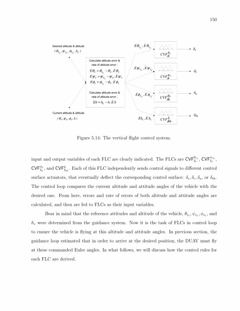
150

Desired attitude & altitude

eδ

rδ

)h , , ,( cvvv cccφψθ

)h , , ,( vvv φψθ

Current attitude & altitude

Calculate attitude error &

rate of attitude error ;

v

.

vvv E ,Ec

θθθθ −=

v

.

vvv E ,Ec

ψψψψ −=

v

.

vvv E ,Ec

φφφφ −=

Calculate altitude error &

rate of altitude error ;

hE ,hhEh

.

c −=

aδ

thδ

cc v

.

v E ,E θθ

cc v

.

v E ,E ψψ

cc v

.

v E ,E φφ

c

.

c hE ,Eh

v

eCVF

θ

δ

va

CVFφ

δ

v

rCVF

ψ

δ

h

thCVF

δ

Figure 5.14: The vertical flight control system.

input and output variables of each FLC are clearly indicated. The FLCs are CVFθvcδe

, CVFψvcδr

,

CVFφv

δa, and CVFhδth . Each of this FLC independently sends control signals to different control

surface actuators, that eventually deflect the corresponding control surface: δe, δr, δa, or δth.

The control loop compares the current altitude and attitude angles of the vehicle with the

desired one. From here, errors and rate of errors of both altitude and attitude angles are

calculated, and then are fed to FLCs as their input variables.

Bear in mind that the reference attitudes and altitude of the vehicle, θvc , ψvc , φvc , and

hc were determined from the guidance system. Now it is the task of FLCs in control loop

to ensure the vehicle is flying at this altitude and attitude angles. In previous section, the

guidance loop estimated that in order to arrive at the desired position, the DUAV must fly

at these commanded Euler angles. In what follows, we will discuss how the control rules for

each FLC are derived.

151

5.4.2.1 Low-Speed Tilted Flight Control

In the guidance system, we have described how the low-speed tilted flight was generally per-

formed, how the commanded Euler angels were estimated, guidance rules used, and how

these rules were derived. Here we move on into the actual process of commanding the ve-

hicle control surfaces upon receiving commands from guidance loop. Let’s begin with the

LSTF(FB) first, followed by the LSTF(LR). For continuity, we proceed with the discussion of

the flight case that was already discussed in LSTF(FB) guidance section, where from hovering

at [PN,PE, h]1 = (0 m, 0 m, 60 m), the vehicle is required to hover at a new position of

[PN,PE, h]2 = (100 m, 0 m, 60 m).

Let’s say for a reference position of PN = 100 m, the guidance loop has estimated that

at the beginning of the motion, the appropriate θvc is −15o. That is to say at the moment

when the position error is still immense (PB). As the altitude is maintained, the north motion

of 100 m needs good control of elevator that through dynamical relationships, the commanded

δe is causing the vehicle to reach −15o tilt angle towards the direction of motion. To develop

a rule, consider at a time when θv = −13o. Tilt angle error is, Eθvc = −15o − (−13o) = −2o.

The maximum tilt angle is −15o, hence for the error of −2o, it is considered small, where in

this case we have negative sign of error (NS).

At the same time, suppose the rate of error is NB, which means the error is increasing

towards more negative at a high rate. In other words, this NB rate of error is actually

decreasing the tilt angle, or the body is rotating counterclockwise towards vertical upright

attitude at a high rate. In response to this, the elevator control must counteract to prevent

the tilt angle from dropping to zero. This is done by giving a large positive elevator deflection,

so that it produces negative pitch rate, which consequently will bring the θv towards more

negative. The rule that describes situation is:

IF Eθvc is NS, AND Eθvc is NB, THEN δe is PB

A set of 25 rules were developed in this way, and these rules are given in Table 5.8 where the

152

underlined italic indicates the rule that we have just derived. The control surface mapping

of CVFψvcδe

is shown in Figure 5.15.

Table 5.8: The rule base for LSTF(FB) control in vertical attitude, CVFθvcδe

.

θvc Error,

(Eθvc)

θvc Error Derivative,

ddt

(Eθvc)

NB NS NZ PS PB

NB PB PB PB PS PS

NS PB PB PS PS NZ

NZ PS NZ NZ NZ NS

PS NZ NS NS NB NB

PB NS NS NB NB NB

-1-0.75

-0.5-0.25

00.25

0.50.75

1

-1

-0.75

-0.5

-0.25

0

0.25

0.5

0.75

1

-1

-0.75

-0.5

-0.25

0

0.25

0.5

0.75

1

Eθv

dEθv

δe

Figure 5.15: Input-output mapping surface of CVFθvcδe

.

Another low-speed translation flight is LSTF(LR). Instead of the elevator, the LSTF

153

in sideways direction is controlled by the rudder. In Figure 5.14, it shows the corresponding

FLC that control the rudder is CVFψvcδr

, and this FLC has the input variables of commanded

ψvc error and its rate. The ψvc for a given reference east position was already determined

by the guidance system, and here the task for the CVFψvcδr

module is to ensure the DUAV

will follow this commanded angle and finally to provide appropriate rudder deflection. In the

example for LSTF(LR) guidance, the DUAV was required to move 95 m to the east. In terms

of position coordinates, the vehicle has to translate from an initial position of [PN,PE, h]1 =

(0 m, 0 m, 60 m), to a new position of [PN,PE, h]2 = (0 m, 95 m, 60 m). We demonstrate

how a control rule for δr is obtained.

Let’s start by stating the ψvc was pre-determined for a reference PE = 95 m, and say

it has the value of 12o. Note in this case, the commanded ψvc is positive because in vertical

attitude, tilting to the right is the positive sense of ψv according to the convention used.

Consider when ψv = 1o, the angle error is calculated as Eψvc = 12o - 1o = 11o. This is a huge

error (PB), however if at this moment the vehicle has a large positive vertical yaw rate, any

rudder deflection is not really needed (NZ) to counteract PB angle error. This is because a

high vertical yaw rate is causing ψv to increase, thus bring the current tilt angle towards the

desired one. In terms of fuzzy sets, a high vertical yaw rate causes a NB tilt angle error rate.

This case can be represented in a control rule as follows:

IF Eψvc is PB, AND Eψvc is NB, THEN δr is NZ

The rest of a complete list of 25 control rules for rudder are provided in Table 5.9, with

underlined italic represents the rule we have derived above. In general, most of these rules

are similar to the rules developed for CVFθvcδer

, except some rules on the edges are slightly

different. The difference in some rules can be observed from the two corresponding surface

plots shown in Figures 5.16 and 5.15. From these two figures, we can see the contours on the

right and left edges are not alike.

154

Table 5.9: The rule base for LSTF(LR) control in vertical attitude, CVFψvcδr

.

ψvc Error,

(Eψvc)

ψvc Error Derivative,

ddt

(Eψvc)

NB NS NZ PS PB

NB PB PB PS NZ NZ

NS PB PS NZ NZ NS

NZ PS NZ NZ NZ NS

PS PS NZ NZ NS NB

PB NZ NZ NS NB NB

-1-0.75

-0.5-0.25

00.25

0.50.75

1

-1-0.75

-0.5-0.25

00.25

0.50.75

1

-1

-0.75

-0.5

-0.25

0

0.25

0.5

0.75

1

Eψv

c

dEψv

c

δr

Figure 5.16: Input-output mapping surface of CVFψvcδr

.

5.4.2.2 Ascend and Descend Flight Control

In normal circumstance, the DUAV will take-off vertically from the ground, although take-off

from a movable platform is also possible. A target altitude is assigned to the controller at

155

which the vehicle needs to hover subsequently after take-off finished. In what follows, we will

discuss the control system for both ascend and descend flights that include multiple hovers. A

schematic of the target altitudes during ascending and descending flights are shown in Figure

5.17.

Altitude

time

AscendHoverDescend

altitude_1

altitude_2

altitude_3

Landing_altitude

Figure 5.17: Hovering altitude command.

The vehicle climbs vertically until it reaches the altitude of first hover h1, and continues

to hover at this altitude for a prescribed time. Then the DUAV is commanded to hover at

a higher altitude (h2), and similar to the first hover, the vehicle may also hover at this

second altitude for a period of time. Now in a similar fashion but in a reverse direction, the

DUAV is commanded to hover at a lower altitude of h3, and finally is commanded to land on

the landing platform. The vertical climb from the ground platform to these three hovering

altitudes involves two vertical motions of each ascend and descend flights. The performance

of these vertical motions is dependent on the thrust control.

Thrust control can be achieved via throttle setting. For the DUAV that uses an electri-

cal motor, the throttle setting is simply the voltage control to the power supply. The throttle

controls the amount of voltage from the power supply to the propeller’s rotor, thus control-

ling the amount of thrust produced by the fan. At the same time, through the dynamical

principle dictated in Equation 5.10, the throttle can alter the vertical velocity of the vehicle.

156

In vertical attitude, this vertical velocity may be referred as the altitude rate h, although they

are not exactly the same. However the latter can be obtained through axis transformation of

the former velocity.

As depicted in Figure 5.14, the FLC that controls the throttle is CVFhδth . The inputs to

this FLC module are the altitude error (Ehc) and the rate of which this error occurs (Ehc).

Whereas, the output of this FLC is the throttle setting δth. Since we are using the full

nonlinear equations of motions to model the vehicle, it is not possible to examine the direct

relationship between each variable to other variables that exist in Equation 5.10. However

we can trace out how the throttle setting has control on the vertical velocity.

This can be examined through the expanded u in Equation 5.10, where in the last

expression we can see the angular rotation of the propeller, Ω. The last expression in this

equation basically represents the thrust from the vehicle’s propeller. The thrust is a function

of angular rotation of the propeller as indicated in Equation 5.18, and is reproduced here.

Apart from Ω, the thrust is also a function of propeller performance, CT and its geometrical

characteristic, R.

T = CTπR2ρ(ΩR)2 (5.18)

Whilst both of these parameters are already fixed in the early design stage, the only

possible way to control the thrust by now is through Ω. The angular rotation Ω, which is more

conveniently expressed in rotational per minute (RPM) is controlled by the voltage supply to

the rotor. Finally, the voltage magnitude that comes out of the power supply is controlled by

the throttle. Although the term “throttle” is normally associated with the combustion engine,

in this thesis the same term is used to refer the control mechanism of the voltage magnitude

supplied to the propeller’s rotor. Since most of the specifications of fuzzy variables are similar

in all FLCs developed in this thesis, we can proceed with the development of the rule base

for throttle control.

Consider when the DUAV is at rest on the ground (h = 0 m) with its engine is idling,

it is required to take-off and hover at hc = 60 m. Prior to take off, the altitude error is, Ehc =

157

60 m - 0 m = 60 m, and the error rate is still insignificant (NZ). At a glance, this maximum

error (PB) requires the throttle to be adjusted at maximum (PB). Moreover, a higher thrust

is needed at the early stage of take-off to overcome the ground effect. However, setting the

throttle at maximum at this time will jeopardize the motion, and most likely will result in

an unstable flight. Therefore, a moderate (PS) throttle is fine to start the vehicle lifts-off the

ground. A rule can be derived for this moment of flight:

IF Ehc is PB, AND Ehc is NZ, THEN δr is PS

This rule is shown in underlined italic in Table 5.10, together with the rest of 24 rules. The

CVFhδth module gives good performance when symmetrical rules are used. In developing the

FLC for throttle control, care is taken for the requirement of the vehicle to have a minimum

hovering thrust at all times. Therefore, the real value obtained from the defuzzification of

the rule consequent of CVFhδth can be one of the following: increment (PB, PS), decrement

(NB, NS) or almost no change (NZ) to the throttle setting for hover. Figure 5.18 shows the

input-output mapping of FLC used for throttle control. This mapping provides a 3D plot

that shows relationships between inputs and output variables of the CVFhδth module. Also

from this surface plot, the symmetrical contour represents the symmetrical rules that have

been developed.

In the example above, a rule for ascending flight was demonstrated. Now consider a

case of descending flight where from hovering at h = 60 m, the vehicle has to hover at a lower

altitude of h = 5 m. Since the lower altitude is the desired altitude that the DUAV have to

reach, it can be written as the commanded altitude, hc = 5 m. At the time when the vehicle

has just started the descend, say at h = 58 m, the altitude error can be calculated as: Ehc

= 5 m - 58 m = -55 m. This is an immense altitude error, but in the negative sense (NB).

Also at this time, let’s say the rate of error is also very big (NB). A NB rate of error

means the rate at which the error moves to a more negative side is huge. Therefore, the

throttle controller must cause the vehicle to move down at a faster speed. Since the error

is still very big, which is still a long way from the desired 5 m hovering altitude, the fastest

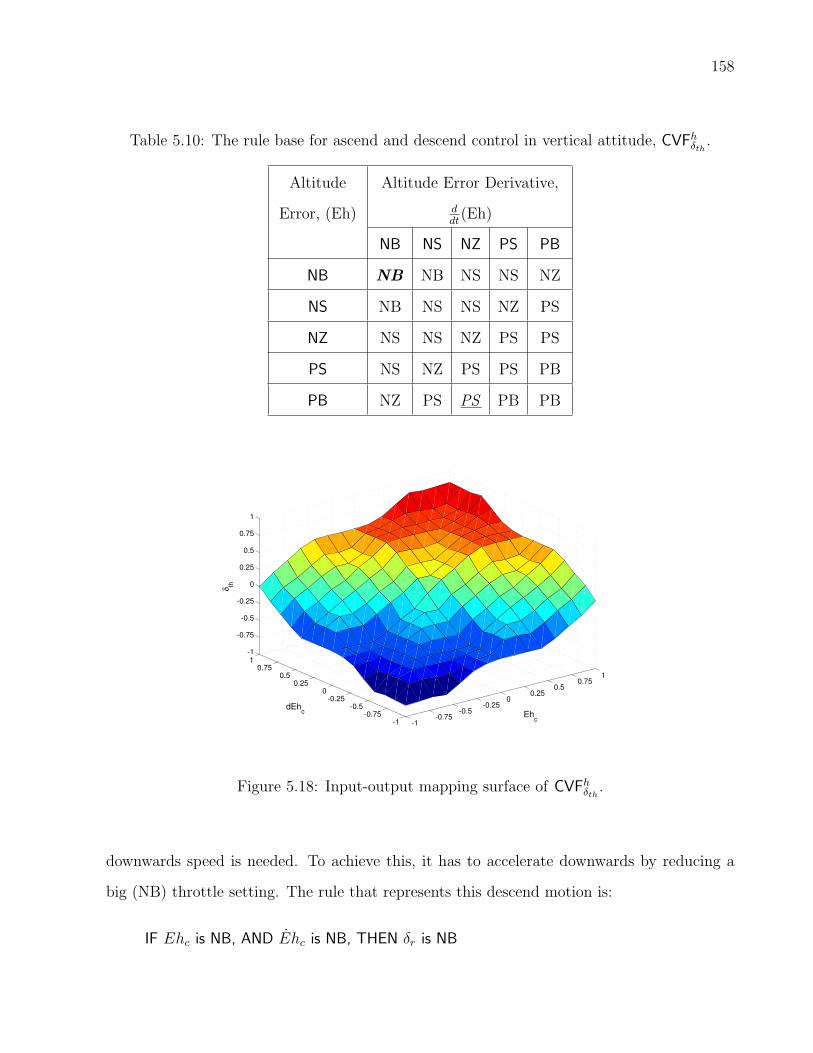
158

Table 5.10: The rule base for ascend and descend control in vertical attitude, CVFhδth .

Altitude

Error, (Eh)

Altitude Error Derivative,

ddt

(Eh)

NB NS NZ PS PB

NB NB NB NS NS NZ

NS NB NS NS NZ PS

NZ NS NS NZ PS PS

PS NS NZ PS PS PB

PB NZ PS PS PB PB

-1-0.75

-0.5-0.25

00.25

0.50.75

1

-1

-0.75

-0.5

-0.25

0

0.25

0.5

0.75

1

-1

-0.75

-0.5

-0.25

0

0.25

0.5

0.75

1

Ehc

dEhc

δth

Figure 5.18: Input-output mapping surface of CVFhδth .

downwards speed is needed. To achieve this, it has to accelerate downwards by reducing a

big (NB) throttle setting. The rule that represents this descend motion is:

IF Ehc is NB, AND Ehc is NB, THEN δr is NB

159

This particular rule is shown in italic bold in Table 5.10. From this it can be deduced that

the developed rule base in Table 5.10, which is for CVFhδth module is to control the throttle in

both ascend and descend flights.

5.4.2.3 Pirouette Control

Pirouette motion is performed when the vehicle needs to change its pointing direction, which

is normally carried out while the vehicle is hovering. This motion is necessary especially prior

to performing LSTF, the vehicle should point at the right direction. This motion can also

be referred as vertical spin. Pirouette is described by the vehicle’s belly pointing angle, or

simply vertical phi, φv. The commanded belly pointing angle, φvc was determined in the

guidance loop. Here, while the vehicle is hovering, the control objective of the FLC is to turn

the vehicle to the commanded pointing angle, φvc by giving appropriate aileron deflection, δa.

The FLC that is responsible to control the aileron during pirouette motion is CVFφv

δa.

Let’s consider a commanded angle, φvc = 45o was given by the guidance system. At

the time when the DUAV was just starting the spin, say at φv = 30, the pointing error

can be calculated as, Eφvc = 45o - 30 = 420. This is a big error (PB). If at this time the

vehicle is having a moderate vertical roll rate, this would physically cause the φv to increase

positively at a moderate rate. In terms of error rate, this positive moderate vertical roll can

be represented by NS φv error rate. It is because as the time increases, the positive roll

would bring φv towards more positive until it goes beyond the commanded φvc , and when

this happens, the φv error would become negative. Although the error is PB, the controller

only needs to command the aileron at a moderate negative level (NS), because the increment

of φv also contributed by the positive body rate. Bear in mind that negative δa always causes

positive φv. Here we have a fuzzy rule as follows:

IF Eφvc is PB, AND Eφvc is NS, THEN δa is NS

This rule is shown in underlined italic in Table 5.11, together with other rules that constitute

a complete 25 rule base for aileron control in the vertical flight. A visualization of a three-

160

dimensional input-output defuzzification surface of CVFφv

δais provided in Figure 5.19. The

asymmetry rules can also be observed from this surface plot by looking at both left and right

portions of this plot.

Table 5.11: The rule base for pirouette control in vertical attitude, CVFφv

δa.

φvc Error,

(Eφvc)

φvc Error Derivative,

ddt

(Eφvc)

NB NS NZ PS PB

NB PB PB PS PS NZ

NS PB PS NZ NZ NS

NZ PS NZ NZ NZ NS

PS PS NZ NZ NS NB

PB NZ NS NS NB NB

-1-0.75

-0.5-0.25

00.25

0.50.75

1

-1-0.75

-0.5-0.25

00.25

0.50.75

1

-1

-0.75

-0.5

-0.25

0

0.25

0.5

0.75

1

Eφv

dEφv

δa

Figure 5.19: Input-output mapping surface of CVFφv

δa.

161

5.5 TRANSITIONS FLIGHT CONTROLLER

The transition flights between horizontal and vertical occurred in a relatively short period

of time. It is the moment when the vehicle rotates about 90o from and to vertical axis. As

described earlier, two transition flights are vertical to horizontal (VtoH), and horizontal to

vertical (HtoV). These maneuvers are mainly governed by longitudinal dynamics, comprising

three degrees of freedom motion in forward, vertical, and pitch directions. The free-body

diagram during the transition flight is shown in Figure 5.20. All forces, moment, and other

flight variables are depicted in the figure. Note also the angle of attack α, pitch angle θ, flight

path angle γ are also shown in the figure.

Figure 5.20: The free-body diagram during transition flight.

The lift and drag shown in Figure 5.20 are the total components that are contributed

from all relevant parts of the body. Here lift and drag forces are included as these forces started

to appear in this type of flight since the dynamic pressure has already built up around the

vehicle body. Indeed, it is essential to maneuver at sufficient dynamic pressure because after

VtoH maneuver was completed, the vehicle is entering the horizontal flight where the vehicle

162

needs to be kept in the air by the lift. The guidance for transition flights is straightforward.

Basically, there are only two variables that are needed to be specified in the transition flights

guidance system:

• VtoH Transition : Initial θ = 90o, Commanded θc = 0o.

• HtoV Transition : Initial θ = 0o, Commanded θc = 90o.

The primary control during transition flights comes from the elevator. The control

objective during transition flight is to provide the appropriate signal to the elevator’s actuator,

through elevator deflection, δe. The vehicle rotates about 900 either from or to vertical axis.

Also, it is required for the vehicle to maneuver with smooth changes in θ. The dynamic

relationship between elevator and body forces and moments is described in the q expanded

expression in Equation 5.14. Since we are using six degrees of freedom nonlinear equations,

we could not obtain a direct one to one relationship between control surface, δe and pitch

rate, q. Nevertheless, in view of FLC, such a relationship is not vital as long as the designed

controller is able to function well.

5.5.1 Vertical to Horizontal Transition Flight Control

The first transition from vertical to horizontal flight occurs after the DUAV has completed

take-off vertically, and needs to enter the high speed horizontal flight phase. A schematic of

this VtoH transition flight is depicted in Figure 5.21. At the end of the vertical flight phase,

the VtoH transition flight is ready to take place as the vehicle increases its flight speed to

gain sufficient dynamic pressure for lifting surfaces to be effective. At this moment while the

thrust is kept constant, the elevator is deflected to create negative pitching moment so that

the whole DUAV body gradually rotates to horizontal axis. In another words, the vehicle’s

centreline is rotated about 90o from the vertical to horizontal plane. The pitch angle, θ is the

variable that is closely monitored during the maneuver.

Once the vehicle’s pitch angle is almost 0o, the authority of the transition flight con-

troller (TFC) is terminated, and the horizontal flight controller (HFC) is in the command.

163

Figure 5.21: A schematic of transition flight from vertical to horizontal.

When θ ∼ 0o, this indicates the completion of the VtoH transition maneuver, and the vehicle

is flying at a nearly constant altitude. As the fan creates forward thrust, the lift is generated

by the wings, tails, and duct, allowing the vehicle to fly forward just like any typical fixed-

wing airplane. In this VtoH transition flight, the corresponding FLC is defined as CVtoHθcδe

.

The first step in VtoH transition is to select a target attitude of pitch angle, θc.

Here, θc = 0o is set as the target attitude for VtoH transition, since prior to this

transition flight the vehicle is in the vertical attitude of θ is 90o. If expressed in vertical Euler

angles, the control task is to bring the DUAV from θv = 0o to θv = −90o. During transition,

the altitude should be maintained, or at least the altitude loss is small. Two input variables

for CVtoHθcδe

, which are pitch angle error and its rate of error. Consider the vehicle is ready to

perform VtoH maneuver and its belly is facing north. At the beginning of the transition, say

at θ = 85o, the angle error is calculated as, Eθ = 0o − 85o = −80o, which can be represented

as NB.

If the NB error is paired with NB rate of error, which results from a high positive

pitch rate, the elevator control has to cause the body to rotate further clockwise. This can be

achieved by deflecting a large positive (PB) δe, because a positive δe decreases the pitch rate.

164

When the vehicle is decreasing in pitch rate, the body tends to pitch down, thus rotating the

vehicle clockwise. This flight scenario can be represented by a fuzzy control rule:

IF Eθc is NB, AND Eθc is NB, THEN δe is PB

The chosen five fuzzy sets for each input variable has led in a 5×5 IF-THEN rule base.

These 25 fuzzy rules include all possible combinations between these two input variables. The

development of these rules is based on the experience and information gathered through the

vehicle simulation. These rules are shown in Table 5.12, with the underlined italic is the

rule that was developed above. The corresponding fuzzy surface plot for CVtoHθcδe

is shown in

Figure 5.22.

Table 5.12: The rule base for VtoH control, CVtoHθcδe

.

Pitch Angle

Error, (Eθc)

Pitch Angle Error

Derivative, ddt

(Eθc)

NB NS NZ PS PB

NB PB PS PS PS NZ

NS PS PS NZ NZ NS

NZ NZ PS NZ NS NS

PS PS NZ NZ NZ NS

PB NZ NS NZ NS NB

5.5.2 Horizontal to Vertical Transition Flight Control

The transition of the DUAV from horizontal to vertical flight is to bring the vehicle back to

hover attitude. It is the reverse of the first transition flight that had been discussed earlier.

The need for the DUAV to be in hover again from high speed horizontal flight is to fulfil the

mission requirement. For example, it is necessary for DUAV to hover over a particular location

165

-1-0.75

-0.5-0.25

00.25

0.50.75

1

-1-0.75

-0.5-0.25

00.25

0.50.75

1

-1

-0.75

-0.5

-0.25

0

0.25

0.5

0.75

1

Eθc

dEθc

δe

Figure 5.22: Input-output mapping surface of CVtoHθcδe

.

to carry out a task like transmitting high quality video surveillance to the ground station. It

is also compulsory for the DUAV to be in hovering flight, before it can land vertically on the

landing platform. Figure 5.23 shows the schematic of DUAV in HtoV transition flight.

In horizontal flight, the vehicle gradually decreases its forward velocity until it reaches

the velocity suitable to perform the pull-up maneuver. To initiate HtoV maneuver, the

vehicle’s speed must be slow enough but not too close to the stall speed. This extreme

pull-up maneuver must be carried out in a stable and smooth manner. At this moment,

deflecting the elevator is decreasing the kinetic energy (speed reduced), but at the same time

increasing the potential energy of the vehicle (altitude gained). The elevator, δe deflects to the

negative side in order to create positive pitching moment which causes the vehicle to rotate

counterclockwise, and end up in vertical attitude. Once the vehicle is in the vertical attitude,

where the pitch angle, θ is about 90o, the authority of HtoV control module is terminated,

and replaced with VFC.

There will be trade-off between the maneuver speed and the undesirable altitude gained

166

Figure 5.23: A schematic of transition flight from horizontal to vertical.

during the HtoV transition flight. A too high speed will result in a higher hovering altitude

and possibly end up with unstable flight, whereas if the speed is to low, the vehicle may

enter the unrecovered stall region. This conflicting factor is an example that justifies the

reason for using fuzzy logic controller. This is because the fuzziness elements in fuzzy logic

will address such matters linguistically and numerically. While elevator controls the HtoV

transition flight, all other control surfaces related to directional and lateral motions are kept

at a neutral state. This can be achieved by rudder and aileron controls that are commanded

to negate any motions from the vertical plane. By doing this, a HtoV maneuver in vertical

plane can be assured.

The FLC module that control the elevator during HtoV is CHtoVθcδe

. Inputs to this FLC

module are pitch angle error and its rate. Five linguistic fuzzy sets were assigned to represent

input and output variables, and triangular membership functions were chosen. Consider at

the beginning of the HtoV flight when θ is 5o, then the pitch angle error is, Eθ = 90o − 50 =

850 (PB). Also at the time when this error occurs, the vehicle is experiencing a high negative

pitch rate, which causes the DUAV to pitch down further. In terms of error rate, this pitch

167

down would cause a PB pitch angle error rate. To correct this, the elevator must be deflected

towards a large negative (NB), so that a large positive pitch rate is developed, and this would

cancel the vehicle tendency to pitch down. A rule can be derived following this flight case:

IF Eθ is PB, AND Eθ is PB , THEN δe is NB

The contradiction in the controller’s objectives of CVtoHθcδe

and CHtoVθcδe

is explained in terms

of the difference of the fuzzy rules developed for these two FLC modules. Now we have to

develop rules that can bring θv from −90o back to 0o. A complete set of fuzzy rules for

CHtoVθcδe

is shown in Table 5.13. Since we have five fuzzy sets on each input, the maximum

number of rules that can be produced are 5×5 = 25. These symmetrical rules provide a better

response in CHtoVθcδe

module compared to asymmetrical rules. The rule that was discussed

above is depicted in underlined italic.

Table 5.13: The rule base for HtoV control, CHtoVθcδe

.

Pitch Angle

Error, (Eθ)

Pitch Angle Error

Derivative, ddt

(Eθ)

NB NS NZ PS PB

NB PB PS PS PS NZ

NS PS PS NZ NZ NS

NZ PS NZ NZ NZ NS

PS PS NZ NZ NS NS

PB NZ NS NS NS NB

5.6 HORIZONTAL FLIGHT CONTROLLER

The horizontal flight of the DUAV includes straight and level flight, bank, and turn. Basically

it covers all flight motions related to any fixed-wing aircraft. Since the current aerodynamic

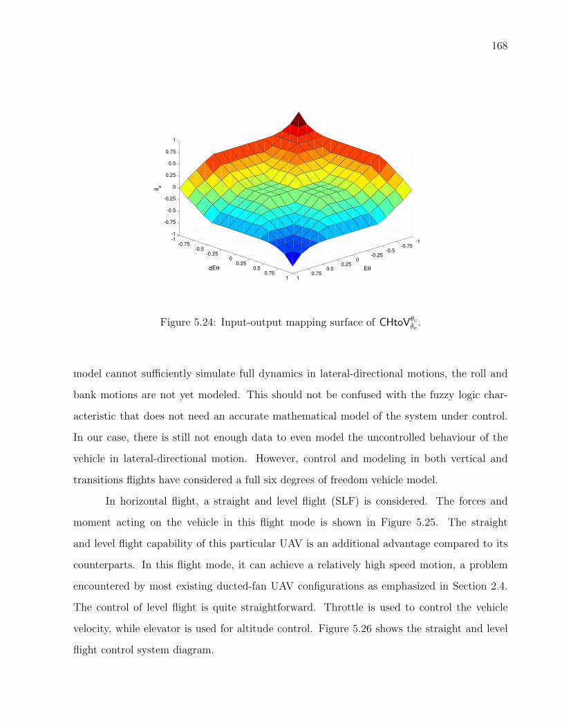
168

-1-0.75

-0.5-0.25

00.25

0.50.75

1

-1

-0.75

-0.5

-0.25

0

0.25

0.5

0.75

1

-1

-0.75

-0.5

-0.25

0

0.25

0.5

0.75

1

EθdEθ

δe

Figure 5.24: Input-output mapping surface of CHtoVθcδe

.

model cannot sufficiently simulate full dynamics in lateral-directional motions, the roll and

bank motions are not yet modeled. This should not be confused with the fuzzy logic char-

acteristic that does not need an accurate mathematical model of the system under control.

In our case, there is still not enough data to even model the uncontrolled behaviour of the

vehicle in lateral-directional motion. However, control and modeling in both vertical and

transitions flights have considered a full six degrees of freedom vehicle model.

In horizontal flight, a straight and level flight (SLF) is considered. The forces and

moment acting on the vehicle in this flight mode is shown in Figure 5.25. The straight

and level flight capability of this particular UAV is an additional advantage compared to its

counterparts. In this flight mode, it can achieve a relatively high speed motion, a problem

encountered by most existing ducted-fan UAV configurations as emphasized in Section 2.4.

The control of level flight is quite straightforward. Throttle is used to control the vehicle

velocity, while elevator is used for altitude control. Figure 5.26 shows the straight and level

flight control system diagram.

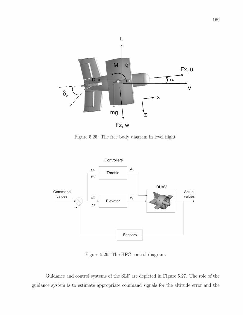
169

Figure 5.25: The free body diagram in level flight.

Controllers

DUAV

Command

values

Actual

values

-

+

thδ

eδEh

EV

VE&

Elevator

hE&

Throttle

Sensors

Figure 5.26: The HFC control diagram.

Guidance and control systems of the SLF are depicted in Figure 5.27. The role of the

guidance system is to estimate appropriate command signals for the altitude error and the

170

velocity error that are needed by the control loop. Altitude error (Eh) and its rate (Eh) are

calculated by making a comparison between the desired and the actual values. Then, Eh and

Eh are sent to the corresponding FLC for altitude control, CHFhδe . Similarly, a comparison is

made between desired and actual velocity in order to calculate any error. Next, the calculated

velocity error (EV ) and its rate (EV ) are sent to the FLC for velocity control, CHFVδth .

Desired altitude & velocity

eδ

)V ,h( cc

V) ,h(

Current altitude & velocity

Calculate velocity error &

rate of velocity error ;

VE ,VVEV

.

c −=

Calculate altitude error &

rate of altitude error ;

hE ,hhEh

.

c −=

thδ

hE ,Eh

.

GUIDANCE

CONTROL

VE ,EV

.

h

eCHF

δ

V

thCHF

δ

Figure 5.27: Guidance and control of the SLF.

5.6.1 Altitude Control

Consider a case where the DUAV is initially flying at the altitude of 50 m, before being

commanded to climb to 100 m and to resume the SLF thereafter. At the time when the

command is received, the altitude error is calculated as, Eh = 100 m - 50 m = 50 m. This

error is still substantial (PB), and is the altitude error rate (PB) as well. To climb, the

vehicle has to deflect the elevator in the negative sense. Therefore, in response to this PB

altitude error, the fuzzy controller (CHFhδe) reacts by commanding a NB elevator deflection.

Following the standard convention of control surfaces deflection, a negative δe results in a

171

positive pitching moment, thus causing the vehicle to climb. A rule can be developed to

represent this situation:

IF Eh is PB, AND Eh is PB, THEN δe is NB

By using the same procedure, the remaining 24 rules are developed from each combination of

fuzzy set in the first and second inputs of CHFhδe . The complete set of 25 fuzzy rules is given

in Table 5.14 with underlined italic indicating the consequence of fuzzy rules derived at this

point. The control surface mapping for of CHFhδe is shown in Figure 5.28.

Table 5.14: The rule base for SLF control, CHFhδe .

Altitude

Error, (Eh)

Altitude Error Derivative,

ddt

(Eh)

NB NS NZ PS PB

NB PB PB PS NZ NZ

NS PS PS NZ NS NS

NZ PS NZ NZ NZ NS

PS PS PS NZ NS NS

PB NZ NS NS NB NB

5.6.2 Velocity Control

The vehicle’s velocity in the SLF is controlled by the throttle setting. Let’s consider a case

when the DUAV is required to reduce its speed from 45 m/s to 30 m/s. Such a case is

necessary prior to the HtoV maneuver where the vehicle should not fly too fast to ensure good

control and to avoid excessive altitude gain at the end of the maneuver. At this moment,

the velocity error can be calculated as, EV = 30 m/s − 45 m/s = −15 m/s. This error is

considered substantial (NB), considering the rate of error is PB. The PB velocity error rate

172

-1

-0.75

-0.5

-0.25

0

0.25

0.5

0.75

1

-1

-0.75

-0.5

-0.25

0

0.25

0.5

0.75

1

-1

-0.75

-0.5

-0.25

0

0.25

0.5

0.75

1

EhdEh

δe

Figure 5.28: Input-output mapping surface of CHFhδe .

means the change of error towards the positive side is immense. In other words, even though

the current velocity is higher than the desired one, the vehicle is experiencing a high rate

of deceleration. Therefore, the appropriate response of the throttle controller (CHFVδth) is to

lower the δth a little bit more (NS). The control law representing this situation is:

IF EV is NB, AND EV is PB, THEN δth is NS

Although the current velocity error is big, the reduction of the throttle setting is not neces-

sarily big since the high rate of deceleration that the vehicle experiences also helps reduce the

vehicle’s speed. The next 24 fuzzy rules are developed in the same manner, where all possible

combinations of current error and their rate are considered. These rules are given in Table

5.15, where the underlined italic indicates the fuzzy rule that we have just derived. Finally,

Figure 5.29 shows the corresponding control surface mapping for CHFVδth .

173

Table 5.15: The rule base for SLF control, CHFVδth .

Velocity

Error, (EV )

Velocity Error Derivative,

ddt

(EV )

NB NS NZ PS PB

NB NB NB NS NS NS

NS NB NS NS NZ NZ

NZ NS NS NZ PS PS

PS NZ NZ PS PS PB

PB PS PS PS PB PB

-1-0.75

-0.5-0.25

00.25

0.50.75

1

-1

-0.75

-0.5

-0.25

0

0.25

0.5

0.75

1

-1

-0.75

-0.5

-0.25

0

0.25

0.5

0.75

1

EVdEV

δth

Figure 5.29: Input-output mapping surface of CHFVδth .

5.7 CONTROLLERS TRANSITION

In a semi or fully autonomous mission, it involves controlling a number of flight modes

seamlessly. In consequence to this situation, of a series of FLCs correspond to these flight

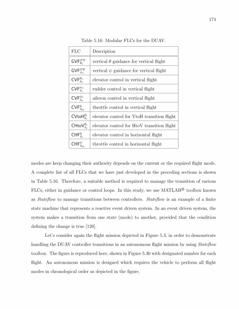
174

Table 5.16: Modular FLCs for the DUAV.

FLC Description

GVFPNθvvertical θ guidance for vertical flight

GVFPEψvvertical ψ guidance for vertical flight

CVFθvδe

elevator control in vertical flight

CVFψv

δrrudder control in vertical flight

CVFφv

δaaileron control in vertical flight

CVFhδth throttle control in vertical flight

CVtoHθcδe

elevator control for VtoH transition flight

CHtoVθcδe

elevator control for HtoV transition flight

CHFhδe elevator control in horizontal flight

CHFVδth throttle control in horizontal flight

modes are keep changing their authority depends on the current or the required flight mode.

A complete list of all FLCs that we have just developed in the preceding sections is shown

in Table 5.16. Therefore, a suitable method is required to manage the transition of various

FLCs, either in guidance or control loops. In this study, we use MATLAB R© toolbox known

as Stateflow to manage transitions between controllers. Stateflow is an example of a finite

state machine that represents a reactive event driven system. In an event driven system, the

system makes a transition from one state (mode) to another, provided that the condition

defining the change is true [120].

Let’s consider again the flight mission depicted in Figure 5.3, in order to demonstrate

handling the DUAV controller transitions in an autonomous flight mission by using Stateflow

toolbox. The figure is reproduced here, shown in Figure 5.30 with designated number for each

flight. An autonomous mission is designed which requires the vehicle to perform all flight

modes in chronological order as depicted in the figure.

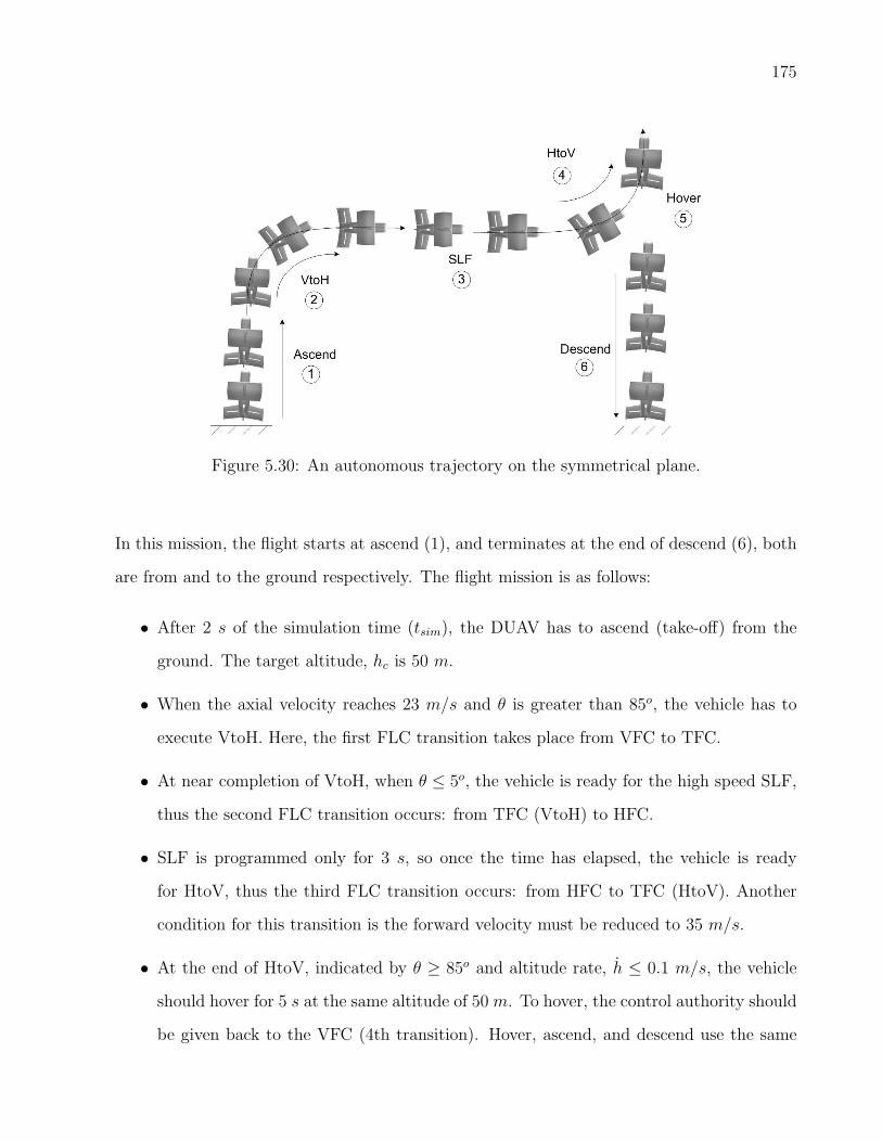
175

Figure 5.30: An autonomous trajectory on the symmetrical plane.

In this mission, the flight starts at ascend (1), and terminates at the end of descend (6), both

are from and to the ground respectively. The flight mission is as follows:

• After 2 s of the simulation time (tsim), the DUAV has to ascend (take-off) from the

ground. The target altitude, hc is 50 m.

• When the axial velocity reaches 23 m/s and θ is greater than 85o, the vehicle has to

execute VtoH. Here, the first FLC transition takes place from VFC to TFC.

• At near completion of VtoH, when θ ≤ 5o, the vehicle is ready for the high speed SLF,

thus the second FLC transition occurs: from TFC (VtoH) to HFC.

• SLF is programmed only for 3 s, so once the time has elapsed, the vehicle is ready

for HtoV, thus the third FLC transition occurs: from HFC to TFC (HtoV). Another

condition for this transition is the forward velocity must be reduced to 35 m/s.

• At the end of HtoV, indicated by θ ≥ 85o and altitude rate, h ≤ 0.1 m/s, the vehicle

should hover for 5 s at the same altitude of 50 m. To hover, the control authority should

be given back to the VFC (4th transition). Hover, ascend, and descend use the same

176

FLC, except the target altitude in each case is different. Thus, for hover, a new hc is

commanded, which is set at the current altitude. In this case, it is 50 m.

• Finally, after 5 s hovering time elapses, the vehicle is commanded to descend or land

by setting hc to zero. The mission is accomplished.

For the practical purpose, several restrictions have been imposed in the simulation loop in

order to change the flight mode. For example, the VtoH maneuver starts at an appropriate

vertical speed of 23 m/s. At this velocity, the effect of freestream dynamic pressure is about

to develop, and this is needed, at least during the second half of the VtoH maneuver to ensure

a smooth transient from the thrust-based to the lift-based motion. For the reverse maneuver,

the vehicle has to slow down to 35 m/s before commanding the HtoV maneuver. This is the

near stall speed of the vehicle, and is required to avoid an excessive altitude gain at the end

of the HtoV maneuver.

Stateflow conditions for the DUAV controller transitions in this example are given in

Table 5.17. In the first column, flight modes are put in a sequence that corresponds to the

chronological order as depicted in Figure 5.30. However, in the last three rows are other flight

modes that are not included in this flight mission. The corresponding FLC for each flight

mode is provided in the last column in Table 5.17. In every flight mode, a unique Stateflow

signal (sf) number is designated. The sf signal will only take the designated number if the

logic state of condition variables are true. To have a true logic, these condition variables have

to reach specific preset values, which depend on the flight missions.

Stateflow toolbox offers a graphical representation of the flight mode logic. This can be

seen in the screenshot of the Stateflow diagram for this mission as shown in Figure 5.31. Each

block represents a flight mode, with the Stateflow signal being stated inside. Neutral block

is the starting point where the simulation begins, and the arrow together with the logical

expression represent the true condition for the corresponding sf signal to be selected. As

indicated in the incoming signal to Neutral block, the simulation should stop when the vehicle

reaches the ground (h= 0m). Note that the tsim settings for both SLF and hover are measured

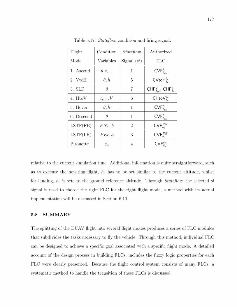
177

Table 5.17: Stateflow condition and firing signal.

Flight Condition Stateflow Authorized

Mode Variables Signal (sf) FLC

1. Ascend θ, tsim 1 CVFhδth

2. VtoH θ, h 5 CVtoHθcδe

3. SLF θ 7 CHFVδth , CHFhδe

4. HtoV tsim, V 6 CHtoVθcδe

5. Hover θ, h 1 CVFhδth

6. Descend θ 1 CVFhδth

LSTF(FB) PNc, h 2 CVFPNδe

LSTF(LR) PEc, h 3 CVFPEδr

Pirouette φv 4 CVFφv

δa

relative to the current simulation time. Additional information is quite straightforward, such

as to execute the hovering flight, hc has to be set similar to the current altitude, whilst

for landing, hc is sets to the ground reference altitude. Through Stateflow, the selected sf

signal is used to choose the right FLC for the right flight mode, a method with its actual

implementation will be discussed in Section 6.10.

5.8 SUMMARY

The splitting of the DUAV flight into several flight modes produces a series of FLC modules

that subdivides the tasks necessary to fly the vehicle. Through this method, individual FLC

can be designed to achieve a specific goal associated with a specific flight mode. A detailed

account of the design process in building FLCs, includes the fuzzy logic properties for each

FLC were clearly presented. Because the flight control system consists of many FLCs, a

systematic method to handle the transition of these FLCs is discussed.

178

DU_auto_sf/signal_flow

SLF

en:sf=7;

Neutral

HtoV

en:sf=6;

VtoH

en:sfn=5;

Hover

en:sf=1

en:hc=50;

Descend

en:sf=1;

en:hc=0;

Ascend

en:sf=1;

en:hc=50;

[theta<5]

[(hdot>=23)&&(theta>=85)]

[(tsim1>3)&&(V<=35)][tsim>=2]

[h=0]

[tsim2>5]

[(hdot<=0.1)&&(theta>=85)]

Figure 5.31: A Stateflow diagram for an autonomous flight mission.

179

Chapter 6

SIMULATION RESULTS AND DISCUSSION

6.1 INTRODUCTION

This chapter presents a large amount of vehicle simulation results. The simulation uses the

vehicle dynamics model that was developed in Chapter 4. The individual simulations based

on flight modes are presented and discussed, followed with results discussion on the fully

autonomous flight simulation combining most of the individual flight modes. The simulation

was conducted using MATLAB R© and Simulink R©. Three MATLAB R© toolboxes were used:

Aerospace Blockset, Fuzzy Logic, and Stateflow.

6.2 A RESULTS GUIDE

A large amount of the DUAV simulation works was done in this study, and the results are

presented in this chapter. Before going through all these results that are presented in the

form of plotted graphs and tables, it seems beneficial to have an overview on how the results

are arranged and discussed. For convenience and good flow of analysis, the simulation results

are divided into four major sections. The first three sections are the discussion and analysis

of simulation results for the individual flight type, and are categorized as: vertical flight,

transition flight, and horizontal flight.

In the vertical flight and transition flight sections, simulation results are further divided

into several subsections based on the flight variations under these main flight modes. In each

main section, it begins with the description of simulation settings for initial conditions and

command signals. Then, the scaling factors for all corresponding FLCs are given. The effect

of scaling factors variation on the system’s performance is demonstrated in the transition

180

flight section.

The evaluation of vehicle stability is based on the fundamental principle of stability.

It is based on the criterion that for a system to be stable, the output response should be

bounded if the system is given with a bounded input. Since inputs in these simulations are

all bounded signals, the stability of the vehicle is guaranteed if the output responses are also

bounded.

In general, five plots are presented and discussed: vehicle position in NED frame, Euler

angles, vehicle’s velocity, control surface deflections, and trajectory model. In some parts,

the corresponding aerodynamic forces and moments are also presented and discussed. In the

horizontal flight simulation, the effect of power setting on the aerodynamic is studied, and

the role of FLC to deal with this interaction is discussed.

Finally, the last major section focuses on results discussion of the vehicle’s autonomous

mission. This section combines all individual flights that were discussed in the first three

sections to form a fully autonomous flight mission, encompassing all flight regimes. The use

of Stateflow toolbox as a mechanism to manage various FLCs systematically is demonstrated

in a greater detail.

6.3 SIMULATION ENVIRONMENT AND SETTINGS

The simulation environment and settings are as follows:

• Atmosphere: A standard atmosphere model is used where atmospheric parameters are

measured at sea level.

• Throttle setting : In vertical flight, the output of the throttle controller is either an

increment or decrement setting from the throttle setting for hover, δhovth .

• Computing machine: The simulation is run on a 2 GB RAM IBM compatible computer.

• Simulation platform: The simulation is run using several computational packages,

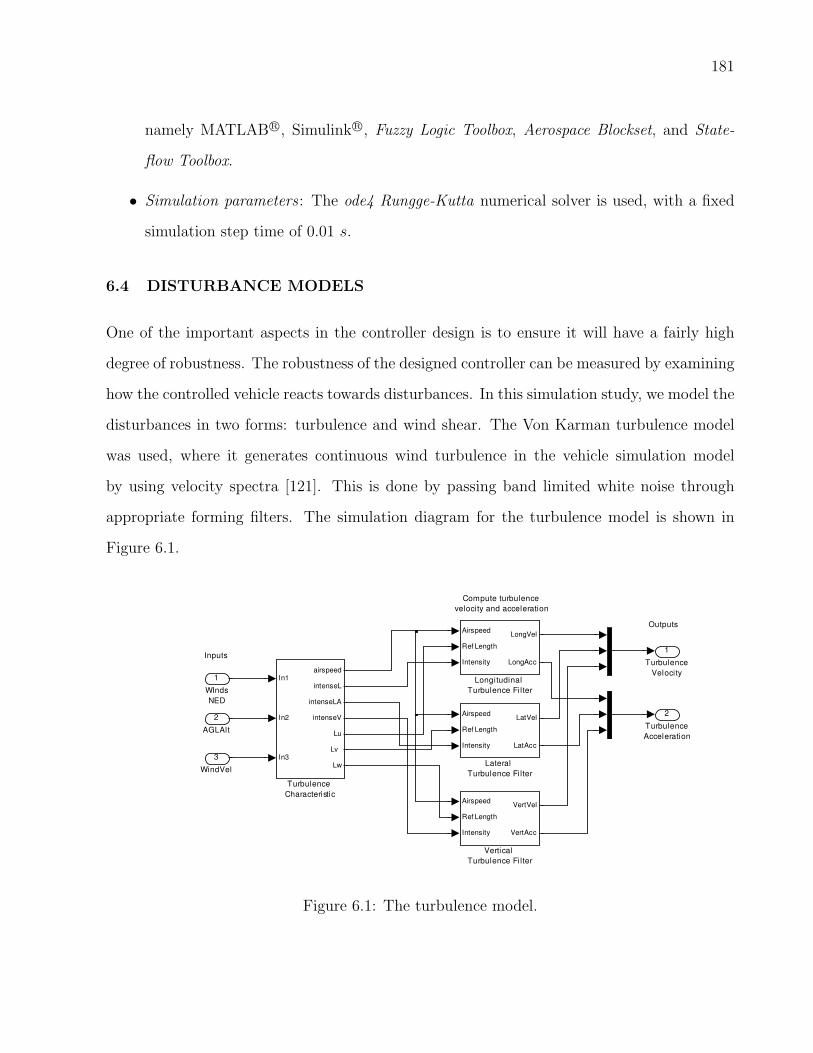
181

namely MATLAB R©, Simulink R©, Fuzzy Logic Toolbox, Aerospace Blockset, and State-

flow Toolbox.

• Simulation parameters : The ode4 Rungge-Kutta numerical solver is used, with a fixed

simulation step time of 0.01 s.

6.4 DISTURBANCE MODELS

One of the important aspects in the controller design is to ensure it will have a fairly high

degree of robustness. The robustness of the designed controller can be measured by examining

how the controlled vehicle reacts towards disturbances. In this simulation study, we model the

disturbances in two forms: turbulence and wind shear. The Von Karman turbulence model

was used, where it generates continuous wind turbulence in the vehicle simulation model

by using velocity spectra [121]. This is done by passing band limited white noise through

appropriate forming filters. The simulation diagram for the turbulence model is shown in

Figure 6.1.

Outputs

Compute turbulence

velocity and acceleration

Inputs

2

Turbulence

Acceleration

1

Turbulence

Velocity

Airspeed

Ref Length

Intensity

VertVel

VertAcc

Vertical

Turbulence Fi lter

In1

In2

In3

airspeed

intenseL

intenseLA

intenseV

Lu

Lv

Lw

Turbulence

Characteristic

Airspeed

Ref Length

Intensity

LongVel

LongAcc

Longitudinal

Turbulence Fi lter

Airspeed

Ref Length

Intensity

LatVel

LatAcc

Lateral

Turbulence Fi lter

3

WindVel

2

AGLAlt

1

WInds

NED

Figure 6.1: The turbulence model.

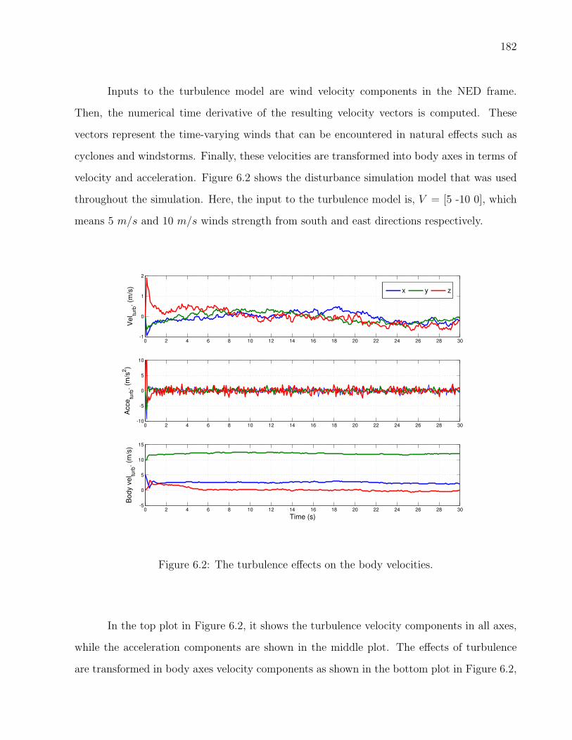
182

Inputs to the turbulence model are wind velocity components in the NED frame.

Then, the numerical time derivative of the resulting velocity vectors is computed. These

vectors represent the time-varying winds that can be encountered in natural effects such as

cyclones and windstorms. Finally, these velocities are transformed into body axes in terms of

velocity and acceleration. Figure 6.2 shows the disturbance simulation model that was used

throughout the simulation. Here, the input to the turbulence model is, V = [5 -10 0], which

means 5 m/s and 10 m/s winds strength from south and east directions respectively.

0 2 4 6 8 10 12 14 16 18 20 22 24 26 28 30-1

0

1

2

Ve

l turb

. (m

/s)

0 2 4 6 8 10 12 14 16 18 20 22 24 26 28 30-5

0

5

10

15

Bo

dy v

el tu

rb. (m

/s)

Time (s)

0 2 4 6 8 10 12 14 16 18 20 22 24 26 28 30-10

-5

0

5

10

Acce

turb

. (m

/s2)

x y z

Figure 6.2: The turbulence effects on the body velocities.

In the top plot in Figure 6.2, it shows the turbulence velocity components in all axes,

while the acceleration components are shown in the middle plot. The effects of turbulence

are transformed in body axes velocity components as shown in the bottom plot in Figure 6.2,

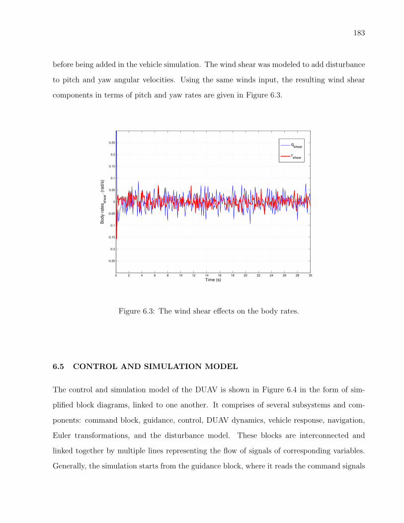
183

before being added in the vehicle simulation. The wind shear was modeled to add disturbance

to pitch and yaw angular velocities. Using the same winds input, the resulting wind shear

components in terms of pitch and yaw rates are given in Figure 6.3.

0 2 4 6 8 10 12 14 16 18 20 22 24 26 28 30

-0.25

-0.2

-0.15

-0.1

-0.05

0

0.05

0.1

0.15

0.2

0.25

Bo

dy r

ate

ssh

ea

r. (r

ad

/s)

Time (s)

qshear

rshear

Figure 6.3: The wind shear effects on the body rates.

6.5 CONTROL AND SIMULATION MODEL

The control and simulation model of the DUAV is shown in Figure 6.4 in the form of sim-

plified block diagrams, linked to one another. It comprises of several subsystems and com-

ponents: command block, guidance, control, DUAV dynamics, vehicle response, navigation,

Euler transformations, and the disturbance model. These blocks are interconnected and

linked together by multiple lines representing the flow of signals of corresponding variables.

Generally, the simulation starts from the guidance block, where it reads the command signals

184

and other necessary information.

EulerEulerV

Vertical Euler

Response

NED

sf

EulerV_c

dth

Guidance

VelWind

alt

Turb. vel

disturb rate

Disturbance

WindD

Control

disturb rate

Tsim

body rates

Euler

NED

VelWind

Prop

Ady

DUAV

tsim

theta

hdot

V

sf

Controllers Transiton

dth

EulerV

sf

EulerV_c

Control

ControlClock

Figure 6.4: The fuzzy logic control scheme on the DUAV.

The information included in the guidance block can range from a simple input to test

the controller, to complete control and guidance commands for a fully autonomous mission.

Inputs from the command block are needed by the guidance system, which later will guide the

controller to generate the appropriate signal to the control surfaces actuator. In response to

this, the vehicle dynamics reacts accordingly, and as a result, one or more control surfaces will

be deflected. This is the time when the numerical integration takes place to solve numerous

equations discussed in Chapter 4: forces and moments, kinematics, and navigation. Then, a

large collection of system responses or outputs are located in the system response block for

easier handling.

185

As we have discussed in Section 4.4, transformations between normal Euler and vertical

Euler are carried out as necessary in representing the vehicle attitude, and these transforma-

tions are included in the Euler block. One of the elements that measures the reliability of the

controller is its ability in disturbance rejection. For this purpose, the modeled disturbances

described in the preceding section were embedded in the vehicle simulation model. Note that

each block in Figure 6.4 also contains its own subsystems and component details, and may

be presented and discussed when necessary.

In the controller transition block, the Stateflow toolbox is used to manage numerous

transitions between FLCs, and also to handle several simulation variables such as assigning

different hc in ascend, descend, and hover. This technique was described in greater details

in Section 5.7, and later in Section 6.10, the actual implementation of such method becomes

apparent. The guidance and control simulation diagrams are shown in more detail in Figure

6.5. The guidance block provides the necessary signal to the control block, and both are linked

as shown at the top part of the figure. Simulation subsystems contained in the guidance and

control blocks are presented at the bottom of each block.

Each shaded block represents a FLC, and the diagram clearly shows that the flight

simulation model has six FLCs, two in the guidance block, and four in the control block

respectively. Note on each FLC, there is a sf input signal from Stateflow. An example of

FLC is shown in Figure 6.6, the module that is responsible to control the elevator deflection,

known as GVFPEψv.

In this figure, we can examine the actual implementation of controller transitions,

where the sf signal from Stateflow is used to determine the right FLC that corresponds to the

current flight mode. Seven FLCs are depicted: four (gray FLCs) are for vertical flight, two

for transition flight (VtoH and HtoV), and one for straight and level flight (SLF). This FLC

simulation diagram indicates the position error and its rate are calculated from the difference

between the commanded and the actual signal. Fuzzy logic scaling factors for both input and

output are clearly shown. Note that these scaling factors are differ according to the flight

186

6

h

5

Vc1

4

hc

3

Control2

EulerV_c

1

Control

Surface

hc

alt

Vc

V

sf

del_th

throttle

sfhc

Vc

thr_guide

PE

sf

psiV_c

rudder_guide

psiV

psiV_c

sf

del_r

rudder

theta_v

thetaV_c

sf

del_e

elevatorPN

sf

thetaV_c

elev_guide

phiV

phiV_c

sf

del_a

aileron

Guidance1

To Workspace2

ControlW

To Workspace1

Guidance

To File2

Control

To File1

phiV_c

Set belly

Scope1

Scope

NED1

sf1

EulerV_c

hc

Vc1

h

Guidance Subsystem

EulerV_c

hc1

EulerV

Vc

h1

V

Control

Control Subsystem

rad deg

13

sf2

12

V1

11

EulerV

10

sf1

9

h1

8

EulerV_c1

7

V

6

Vc

5

hc1

4

sf

3

EulerV1

2

NED1

1

NED

Figure 6.5: Flight guidance and control diagrams.

mode. As such, these scaling factor blocks are set as dummy variables that will have its value

changed depends on the current flight mode. Also note in the figure, a saturation block is

placed ahead of the FLC output, a method to ensure the resulting output is within the limit.

In general, a similar arrangement of subsystems components is used in all FLCs.

6.6 CONTROLLER RESPONSE

Before the designed controllers are placed in the vehicle simulation model, it is crucial to

test these controllers individually to ensure they functions correctly. Figure 6.7 shows the

response of each controller due to the five units step input. The controller’s performance is

measured in terms of velocity response that corresponds to this command input. For 5o of

δe, the corresponds w is about 5.5 m/s with the rise time about 2.5 s. Rudder has a faster

rise time response, but with a smaller velocity magnitude, where for the same magnitude of

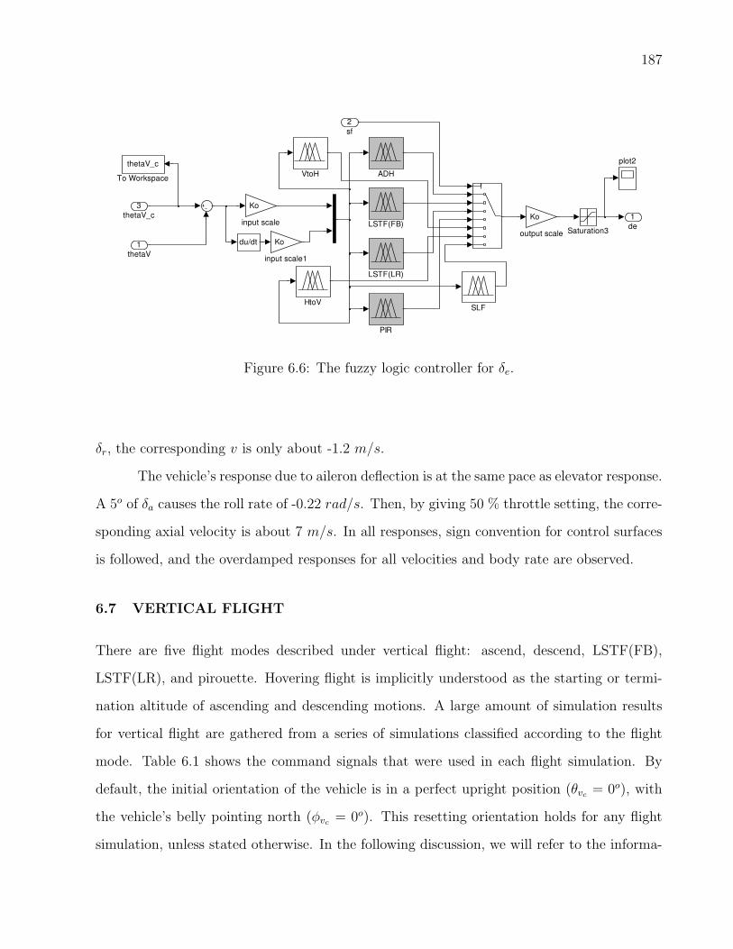
187

1

de

plot2

Ko

output scale

Ko

input scale1

Ko

input scale

VtoH

thetaV_c

To Workspace

Saturation3

SLF

PIR

LSTF(LR)

LSTF(FB)

HtoV

du/dt

ADH

3

thetaV_c

2

sf

1

thetaV

Figure 6.6: The fuzzy logic controller for δe.

δr, the corresponding v is only about -1.2 m/s.

The vehicle’s response due to aileron deflection is at the same pace as elevator response.

A 5o of δa causes the roll rate of -0.22 rad/s. Then, by giving 50 % throttle setting, the corre-

sponding axial velocity is about 7 m/s. In all responses, sign convention for control surfaces

is followed, and the overdamped responses for all velocities and body rate are observed.

6.7 VERTICAL FLIGHT

There are five flight modes described under vertical flight: ascend, descend, LSTF(FB),

LSTF(LR), and pirouette. Hovering flight is implicitly understood as the starting or termi-

nation altitude of ascending and descending motions. A large amount of simulation results

for vertical flight are gathered from a series of simulations classified according to the flight

mode. Table 6.1 shows the command signals that were used in each flight simulation. By

default, the initial orientation of the vehicle is in a perfect upright position (θvc = 0o), with

the vehicle’s belly pointing north (φvc = 0o). This resetting orientation holds for any flight

simulation, unless stated otherwise. In the following discussion, we will refer to the informa-

188

0 0.5 1 1.5 2 2.5 3 3.5 4 4.5 50

2.5

5

δe(o

)

0 0.5 1 1.5 2 2.5 3 3.5 4 4.5 50

2

4

6

8

10

w (

m/s

)

0 0.5 1 1.5 2 2.5 3 3.5 4 4.5 50

2.5

5

δr(o

)

0 0.5 1 1.5 2 2.5 3 3.5 4 4.5 5-2.5

0

2.5

5

v (

m/s

)

0 0.5 1 1.5 2 2.5 3 3.5 4 4.5 50

2.5

5

δa(o

)

0 0.5 1 1.5 2 2.5 3 3.5 4 4.5 5-0.3

-0.2

-0.1

0

p (

rad

/s)

0 0.5 1 1.5 2 2.5 3 3.5 4 4.5 50

25

50

δth

(%)

Time (s)

0 0.5 1 1.5 2 2.5 3 3.5 4 4.5 50

2

4

6

8

10

u (

m/s

)

system responsestep input to controller

Figure 6.7: The controllers test.

tion presented in this table as required. Scaling factors for input and output variables for all

FLCs in the vertical flight simulation are given in Table 6.2.

Table 6.1: Command signals and initial altitude for vertical flight simulation.

Flight Mode Ascend Descend Pirouette LSTF(FB) LSTF(LR)

φvc(o) 0 0 10sin t 0 0

Command hinit(m) 0 50 40 40 40

Signal hc(m) [20,50] 30 40 40 40

PNc(m) 0 0 0 10sin t 0

PEc(m) 0 0 0 0 10sin t

189

Table 6.2: Scaling factors for FLC modules in vertical flight.

Scaling FactorFLC Module

GVFPNθvGVFPEψv

CVFθvδe

CVFψv

δrCVFφv

δaCVFhδth

Input1 0.01 0.04 0.01 0.02 0.02 0.01

Input2 0.09 0.02 0.02 0.01 0.03 0.02

Output 1.5 2 2 9 4 7

6.7.1 Ascend, Hover and Descend Flights

As the nature of flights in ascend, descend, and hover (ADH) are closely related to each

other, it is very convenient to discuss all simulation results from these flights in one section.

Table 6.1 shows the necessary guidance settings for these flight simulations. It requires the

definition of four command signals and three initial conditions which are PNc, PEc, hc, φvc

and hinit respectively, with another two default initial conditions (θvinitand φvinit

) already

mentioned above. The initial altitude, hinit = 0 means the vehicle is initially on the ground.

The zero command signals for PNc, PEc and φvc in both ascend and descend describes that

the vehicle should maintain a zero north and east position, with the belly always pointing

north throughout the flight.

The simulation of ascend, hover, and descend flights is based on hover command signal

in the form of three steps input, hc = [20 m 50 m 30 m]. It simply means the DUAV needs

to hover at three different altitudes. Figure 6.8 shows the corresponding vehicle responses

to this command input. Note in Figure 6.8(a), the command signal is shown with the step

time of 10 s on each hovering altitude. Practically, the step time of 10 s in not necessarily

the actual time needed to stay in hover, rather it states that after 10 s, the vehicle needs to

change its hovering altitude. The time needed for take-off (ascend) and hover are all included

in the allocated time of 10 s.

Starting from rest, but with idling engine on the ground, the DUAV ascends to reach

190

0 2 4 6 8 10 12 14 16 18 20 22 24 26 28 300

10

20

30

40

50

60

70

Altitu

de

(m

)

(a)

0 2 4 6 8 10 12 14 16 18 20 22 24 26 28 30-10

-5

0

5

10

ve

locity (

m/s

)

Time (s)(c)

0 2 4 6 8 10 12 14 16 18 20 22 24 26 28 30-1

-0.5

0

0.5

1

δth

(b)

set

actual

Figure 6.8: Altitude, throttle, and velocity responses in ADH.

the first hovering altitude at 20 m. Figure 6.8(a) depicts a smooth lift off taking about 5

s to reach the first hover. With good command follower is assured, almost no overshoot in

the first and third hover, except an insignificant overshoot has occurred during the ascending

flight to reach the second hover. Figure 6.8(b) shows the throttle setting for this flight, while

Figure 6.8(c) shows the corresponds vertical velocity. Refer back to Table 5.4 in Chapter 5,

the respective FLC for the throttle controller is CVFhδth .

The throttle setting shows a variation of adding (+ve part) and subtracting (-ve part)

to and from the base hover setting. Note at the beginning and at t = 10 s, a steep throttle

(read as thrust) increase is resulted from fuzzy rules in CVFhδth that have reasoned how big

the throttle should be when the target altitude is still too far. In contrast to this, at t = 20

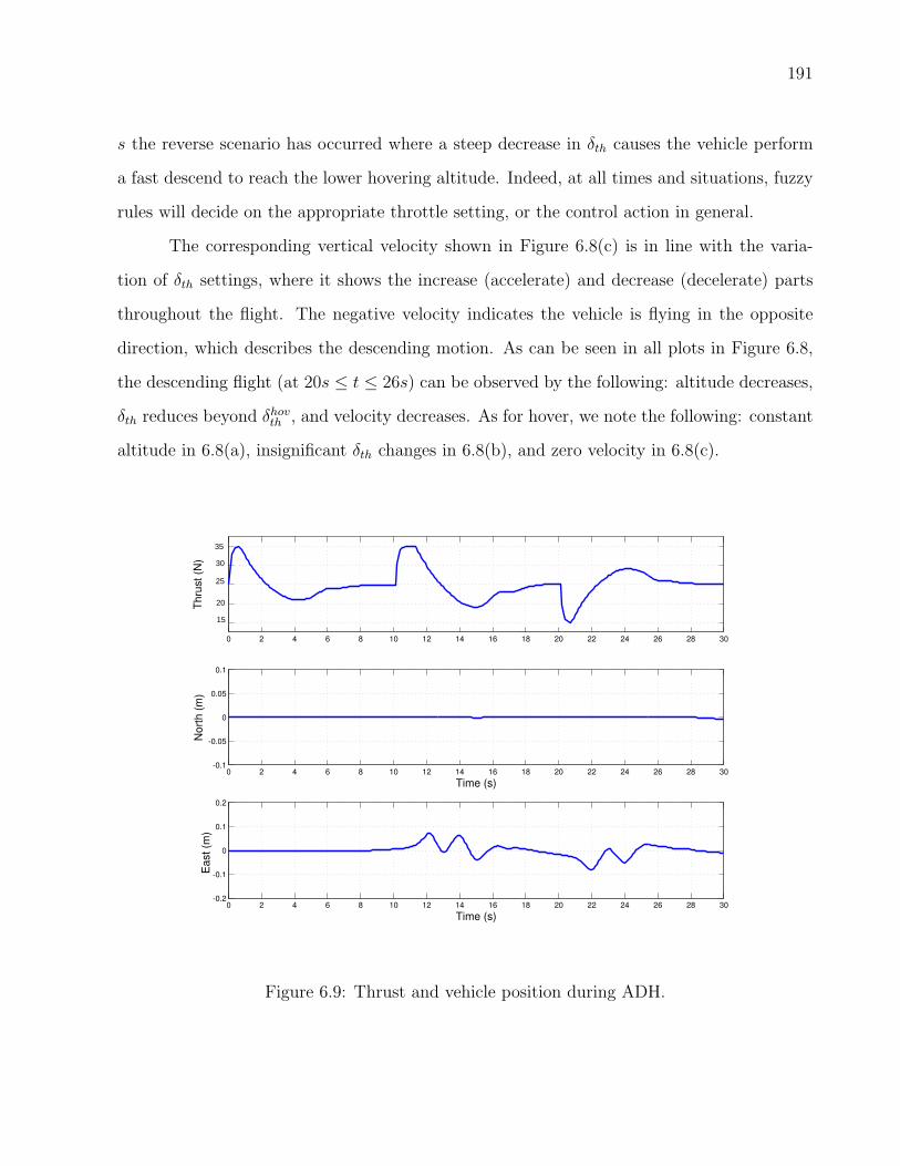
191

s the reverse scenario has occurred where a steep decrease in δth causes the vehicle perform

a fast descend to reach the lower hovering altitude. Indeed, at all times and situations, fuzzy

rules will decide on the appropriate throttle setting, or the control action in general.

The corresponding vertical velocity shown in Figure 6.8(c) is in line with the varia-

tion of δth settings, where it shows the increase (accelerate) and decrease (decelerate) parts

throughout the flight. The negative velocity indicates the vehicle is flying in the opposite

direction, which describes the descending motion. As can be seen in all plots in Figure 6.8,

the descending flight (at 20s ≤ t ≤ 26s) can be observed by the following: altitude decreases,

δth reduces beyond δhovth , and velocity decreases. As for hover, we note the following: constant

altitude in 6.8(a), insignificant δth changes in 6.8(b), and zero velocity in 6.8(c).

0 2 4 6 8 10 12 14 16 18 20 22 24 26 28 30

15

20

25

30

35

Th

rust (N

)

0 2 4 6 8 10 12 14 16 18 20 22 24 26 28 30-0.1

-0.05

0

0.05

0.1

No

rth

(m

)

Time (s)

0 2 4 6 8 10 12 14 16 18 20 22 24 26 28 30-0.2

-0.1

0

0.1

0.2

Ea

st (m

)

Time (s)

Figure 6.9: Thrust and vehicle position during ADH.

192

Two ascend flights were recorded to have maximum vertical velocities of 6 m/s and 8

m−1 respectively. This confirms that the low speed motion in vertical flight was implemented

as expected, which is within the same vertical velocity response presented in the previous

section. Furthermore, the maximum and minimum velocities are directly related to the δth

setting, which later depends on the magnitude of altitude error. Figure 6.9 shows the thrust

and ground reference position during ascend, hover, and descend.

Thrust corresponds to δth setting, while the position in north and east coordinates are

resulted from elevator (CVFθvδe

) and rudder (CVFψv

δr) control during the flight. As noted before,

and now proven that the zero command signal for PNc and PEc means GVFPNθvand GVFPEψv

have ensured the DUAV was flying neither to the north-south nor to the east-west directions.

In figures 6.9(b) and (c), an extremely small deviation either in the north or the east sides

(<8 cm) confirms the vehicle has maintained an almost perfect upright motion throughout

the flight.

Remember that disturbances are present in the simulation model in terms of 5 m/s and

10 m/s northerly and easterly winds respectively. The near zero north and south positions

are evidences of the controller’s ability to perform well in the disturbance rejection. It also

means the vehicle is flying in a stable orientation. This can be clearly seen in Figure 6.10,

where it shows very little error in vertical Euler angles. The controller’s efforts to follow the

command and to maintain the vehicle’s stability can be observed from three plots on the right

side of Figure 6.10. Note that the oscillations in the rudder response (subsequently on ψv)

are due to the 5 m/s westerly wind disturbance.

In this ADH flight, the motions are mainly controlled by the throttle, although elevator,

rudder, and aileron are activated as well. The throttle ensures the main objective of reaching

a series of hovering altitude is achieved, whilst the rest of three control surfaces maintain

the vehicle’s stability and position. In the situation where wind disturbances are weak, these

three controllers are put to “rest” mode during ascend, descend, and hover. Therefore, the

throttle is the dominant controller in ADH motions, a concept explained in Section 5.3.4.

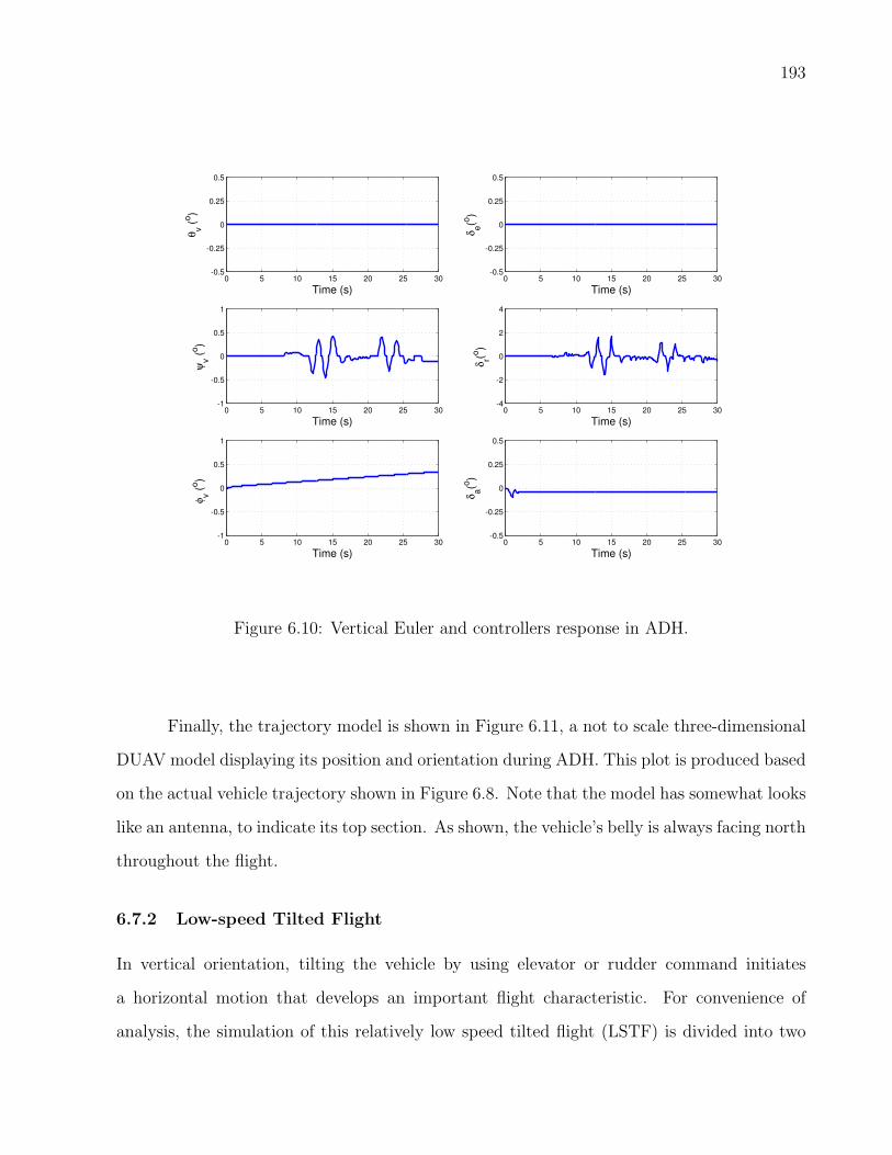
193

0 5 10 15 20 25 30-0.5

-0.25

0

0.25

0.5

θv (

o)

Time (s)

0 5 10 15 20 25 30-0.5

-0.25

0

0.25

0.5

δe(o

)

Time (s)

0 5 10 15 20 25 30-1

-0.5

0

0.5

1

ψv (

o)

Time (s)

0 5 10 15 20 25 30-4

-2

0

2

4

δr(o

)

Time (s)

0 5 10 15 20 25 30-1

-0.5

0

0.5

1

φv (

o)

Time (s)

0 5 10 15 20 25 30-0.5

-0.25

0

0.25

0.5

δa(o

)

Time (s)

Figure 6.10: Vertical Euler and controllers response in ADH.

Finally, the trajectory model is shown in Figure 6.11, a not to scale three-dimensional

DUAV model displaying its position and orientation during ADH. This plot is produced based

on the actual vehicle trajectory shown in Figure 6.8. Note that the model has somewhat looks

like an antenna, to indicate its top section. As shown, the vehicle’s belly is always facing north

throughout the flight.

6.7.2 Low-speed Tilted Flight

In vertical orientation, tilting the vehicle by using elevator or rudder command initiates

a horizontal motion that develops an important flight characteristic. For convenience of

analysis, the simulation of this relatively low speed tilted flight (LSTF) is divided into two

194

Figure 6.11: Trajectory model of ADH.

parts, based on the directions of motion: in forward-backward direction, LSTF(FB), and in

left-right or sideways direction, LSTF(LR). The settings and command signals for the LSTF

simulation is shown in Table 6.1, and can be reiterated as follows:

• The vehicle initially pointing north, hovering at 40 m altitude as hinit is set to 40 m.

• The flight should be made at constant altitude as hc and hinit are both set to 40 m.

• The flight must maintain on a straight path as PEc and PNc are set to 0 for both

LSTF(FB) and LSTF(LR).

• The vehicle must maintain the pointing direction to the north as φv is set to 0.

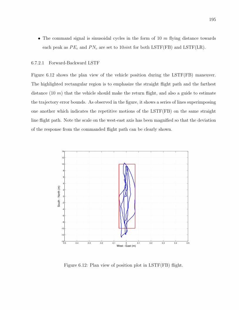
195

• The command signal is sinusoidal cycles in the form of 10 m flying distance towards

each peak as PEc and PNc are set to 10sint for both LSTF(FB) and LSTF(LR).

6.7.2.1 Forward-Backward LSTF

Figure 6.12 shows the plan view of the vehicle position during the LSTF(FB) maneuver.

The highlighted rectangular region is to emphasize the straight flight path and the farthest

distance (10 m) that the vehicle should make the return flight, and also a guide to estimate

the trajectory error bounds. As observed in the figure, it shows a series of lines superimposing

one another which indicates the repetitive motions of the LSTF(FB) on the same straight

line flight path. Note the scale on the west-east axis has been magnified so that the deviation

of the response from the commanded flight path can be clearly shown.

-0.5 -0.4 -0.3 -0.2 -0.1 0 0.1 0.2 0.3 0.4 0.5-14

-12

-10

-8

-6

-4

-2

0

2

4

6

8

10

12

14

So

uth

- N

ort

h (

m)

West - East (m)

Figure 6.12: Plan view of position plot in LSTF(FB) flight.

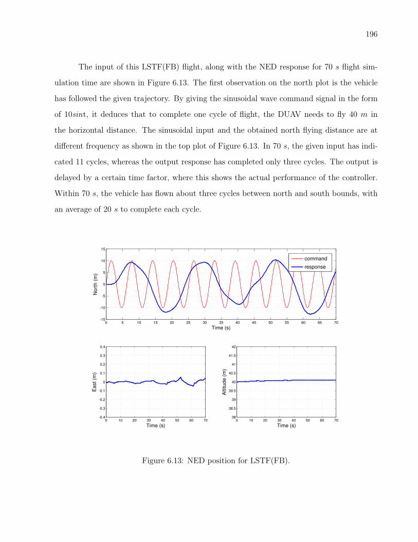
196

The input of this LSTF(FB) flight, along with the NED response for 70 s flight sim-

ulation time are shown in Figure 6.13. The first observation on the north plot is the vehicle

has followed the given trajectory. By giving the sinusoidal wave command signal in the form

of 10sint, it deduces that to complete one cycle of flight, the DUAV needs to fly 40 m in

the horizontal distance. The sinusoidal input and the obtained north flying distance are at

different frequency as shown in the top plot of Figure 6.13. In 70 s, the given input has indi-

cated 11 cycles, whereas the output response has completed only three cycles. The output is

delayed by a certain time factor, where this shows the actual performance of the controller.

Within 70 s, the vehicle has flown about three cycles between north and south bounds, with

an average of 20 s to complete each cycle.

0 5 10 15 20 25 30 35 40 45 50 55 60 65 70-15

-10

-5

0

5

10

15

No

rth

(m

)

Time (s)

0 10 20 30 40 50 60 70-0.4

-0.3

-0.2

-0.1

0

0.1

0.2

0.3

0.4

Ea

st (m

)

Time (s)

0 10 20 30 40 50 60 7038

38.5

39

39.5

40

40.5

41

41.5

42

Altitu

de

(m

)

Time (s)

command

response

Figure 6.13: NED position for LSTF(FB).

197

While there is no visible error on the north side and sideways, it can be observed that

the trajectory is encountering overshoot and undershoot within ± 2 m error bound of the

south side. A few reasons could lead to this error: wind disturbances, improper FLC tuning,

or a combination of both. Even so, this error can still be considered as relatively minor and

is not a major concern since the vehicle demonstrates good flight performance. This can be

evaluated from both altitude and east plots in Figure 6.13, where the altitude of 40 m is

maintained all the way through, and the deviation from the straight path is very little.

The propulsive response for this flight is shown in Figure 6.14 which consists of throttle

setting, engine’s RPM, and thrust. Because the throttle is kept constant throughout the flight,

there is no change in the developed thrust, and consequently the altitude is maintained all

the way through as we have seen in Figure 6.13. Although the propulsive response shows a

bit flutter, it is within a tiny bounds, therefore its effect on the altitude fluctuation is hardly

seen. The FLC module that has ensured the altitude is maintained in this flight is CVFhδth .

The LSTF(FB) is dominantly controlled by the elevator, with the corresponding FLCs

are GVFPNθvand CVFθv

δe. Other controllers are to have function as: rudder to maintain a

straight north-south flight path, aileron to ensure the right pointing angle, and throttle to

maintain the altitude. The results of various responses of elevator deflection, vertical Euler,

and flight velocity are presented in Figure 6.15. A small range of δe (±4o) is in line with the

requirement to have a low speed flight in this tilted orientation. On average, the maximum

flight speed is 3 m/s. Small δe causes a low tilt angle (maximum θv ∼ 7o), and in consequence

to this, a more stable flight is achieved.

The stability of this tilted flight can be observed by examining the aerodynamic mo-

ments that correspond to this flight motion. Figure 6.16 shows the response of all three

moments: roll, pitch, and yaw. As we have seen in Figure 6.13, there is no deviation towards

east because the vehicle does not produce both rolling and yawing moments as shown in Fig-

ure 6.16(a) and Figure 6.16(b). The only useful moment in this flight is pitching, where the

corresponding FLCs (GVFPNθvand CVFθv

δe) have estimated that the pitching moment within ±

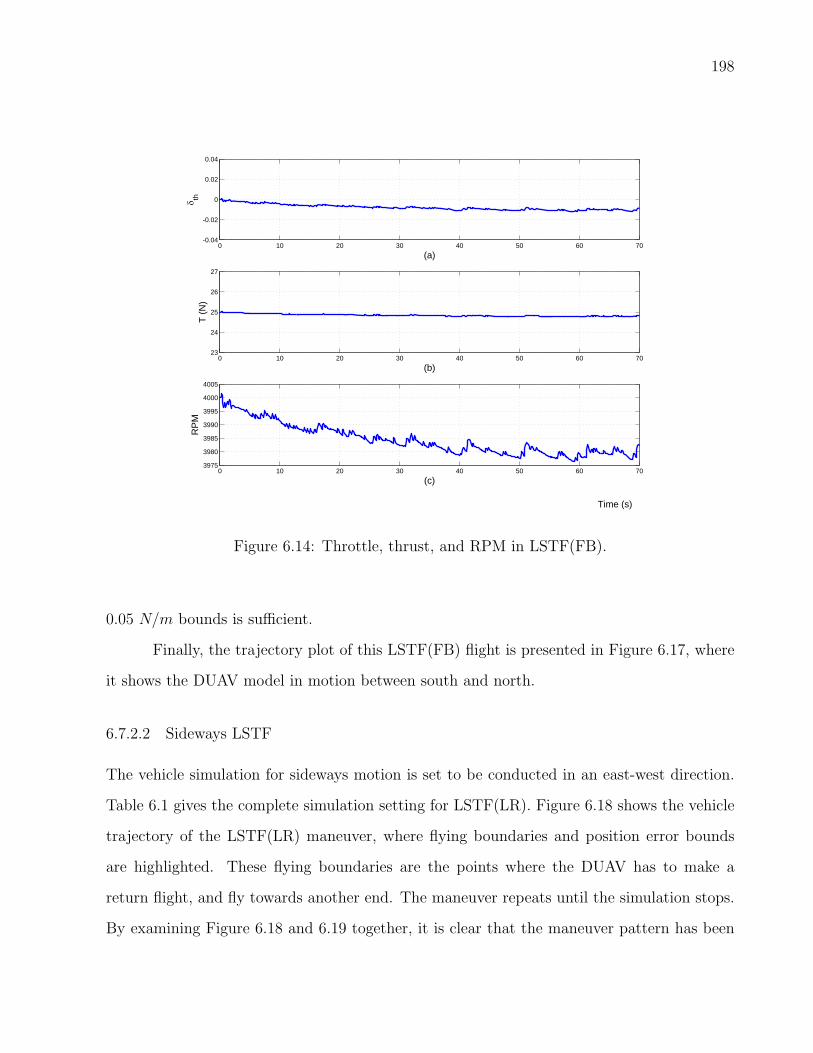
198

0 10 20 30 40 50 60 70-0.04

-0.02

0

0.02

0.04

δ th

(a)

0 10 20 30 40 50 60 7023

24

25

26

27

T (N

)

(b)

0 10 20 30 40 50 60 703975

3980

3985

3990

3995

4000

4005

RPM

(c)

Time (s)

Figure 6.14: Throttle, thrust, and RPM in LSTF(FB).

0.05 N/m bounds is sufficient.

Finally, the trajectory plot of this LSTF(FB) flight is presented in Figure 6.17, where

it shows the DUAV model in motion between south and north.

6.7.2.2 Sideways LSTF

The vehicle simulation for sideways motion is set to be conducted in an east-west direction.

Table 6.1 gives the complete simulation setting for LSTF(LR). Figure 6.18 shows the vehicle

trajectory of the LSTF(LR) maneuver, where flying boundaries and position error bounds

are highlighted. These flying boundaries are the points where the DUAV has to make a

return flight, and fly towards another end. The maneuver repeats until the simulation stops.

By examining Figure 6.18 and 6.19 together, it is clear that the maneuver pattern has been

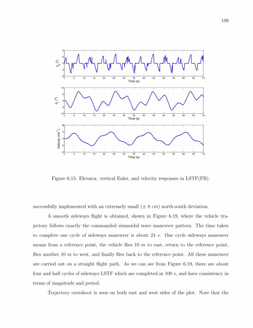
199

0 5 10 15 20 25 30 35 40 45 50 55 60 65 70-6

-3

0

3

6

δe (

o)

Time (s)

0 5 10 15 20 25 30 35 40 45 50 55 60 65 70-10

-5

0

5

10

θv (

o)

Time (s)

0 5 10 15 20 25 30 35 40 45 50 55 60 65 70-6

-3

0

3

66

Ve

locity (

ms

-1)

Time (s)

Figure 6.15: Elevator, vertical Euler, and velocity responses in LSTF(FB).

successfully implemented with an extremely small (± 8 cm) north-south deviation.

A smooth sideways flight is obtained, shown in Figure 6.19, where the vehicle tra-

jectory follows exactly the commanded sinusoidal wave maneuver pattern. The time taken

to complete one cycle of sideways maneuver is about 24 s. One cycle sideways maneuver

means from a reference point, the vehicle flies 10 m to east, return to the reference point,

flies another 10 m to west, and finally flies back to the reference point. All these maneuver

are carried out on a straight flight path. As we can see from Figure 6.19, there are about

four and half cycles of sideways LSTF which are completed in 100 s, and have consistency in

terms of magnitude and period.

Trajectory overshoot is seen on both east and west sides of the plot. Note that the

200

0 10 20 30 40 50 60 70-0.01

-0.005

0

0.005

0.01

l (N

m)

(a)

0 10 20 30 40 50 60 70-0.1

-0.05

0

0.05

0.1

M (N

m)

(b)

0 10 20 30 40 50 60 70-0.04

-0.02

0

0.02

0.04

N (N

m)

(c)Time (s)

Figure 6.16: Aerodynamic moments in LSTF(FB).

Figure 6.17: Trajectory model for LSTF(FB).

201

-18 -16 -14 -12 -10 -8 -6 -4 -2 0 2 4 6 8 10 12 14 16 18-0.4

-0.3

-0.2

-0.1

0

0.1

0.2

0.3

0.4

So

uth

- N

ort

h (

m)

West - East (m)

Figure 6.18: Plan view of position plot in LSTF(LR) flight.

overshoot is bigger on the south side as the vehicle has flown about 5 m (maximum) beyond

the boundary. This overshoot results from moderate wind disturbance present in the system.

In general, the trajectory overshoot or error in this maneuver is on the average of 3 m in each

cycle. To compensate for this error and to sustain a stable flight, the vehicle has to tilt at a

larger ψv compared to the tilt angle in LSTF(FB) flight. The corresponding ψv can be seen

in Figure 6.20, where the vehicle is flying sideways with ±25o tilting angle.

A large ψv is obtained through a larger rudder deflection (±11o). The corresponding

aerodynamic moments for this situation are shown in Figure 6.21. We have learned the

sideways LSTF can only be initiated by yawing moment. For the commanded signal depicted

in Table 6.1, the FLC has estimated that the yawing moment within bounds ± 1 Nm as

shown in Figure 6.21(c) is sufficient.

202

0 5 10 15 20 25 30 35 40 45 50 55 60 65 70 75 80 85 90 95 100100-15

-10

-5

0

5

10

15

Ea

st (m

)

Time (s)

command

response

0 10 20 30 40 50 60 70 80 90 100100-4

-3

-2

-1

0

1

2

3

4

No

rth

(m

)

Time (s)

0 10 20 30 40 50 60 70 80 90 10010030

35

40

45

50

Altitu

de

(m

)

Time (s)

Figure 6.19: NED position for LSTF(LR).

The LSTF(LR) has maintained a low speed flight with the maximum of 5 m/s. Rudder

in the main controller in this flight. It works in the same way as elevator, where its deflection

causes the vehicle to tilt sideways. Subsequently, the thrust vector changes and sideways

motion is initiated. The corresponding FLCs for the rudder control are GVFPEψvand CVFψv

δr

as provided in Table 5.4. From the altitude plot in Figure 6.19, it shows a quite significant

altitude drop (∼ 5 m) from t = 2 s to t = 10 s, before the vehicle climbs back to the desired

altitude.

This altitude drop at the beginning of the simulation is corrected by the δth response

as can be seen in Figure 6.22(a). In response with this altitude drop, the corresponding FLC

was tried to correct this error by increasing δth setting in the first 10 s of the simulation.

203

0 5 10 15 20 25 30 35 40 45 50 55 60 65 70-20

-10

0

10

20

δr (

o)

Time (s)

0 5 10 15 20 25 30 35 40 45 50 55 60 65 70

-25

0

25

ψv (

o)

Time (s)

0 5 10 15 20 25 30 35 40 45 50 55 60 65 70-10

-5

0

5

10

Ve

locity (

m/s

)

Time (s)

Figure 6.20: Rudder, vertical Euler, and velocity responses in LSTF(LR).

Once the altitude is maintained at the desired setting, the δth is back to the normal setting.

In this sideways tilted flight, the fluctuation of the response is a bit bigger than it does in the

forward-backward tilted flight.

The source to this degradation is most likely also due to wind disturbances. On the

other hand, this scenario has demonstrated the ability of the non-dominant controller to

function as expected. In this case, the throttle controller (CVFhδth) has responded to the

altitude loss by increasing the throttle setting (not shown) so that more thrust is produced

and finally the commanded altitude is restored. Although the altitude error still exists, it is

considered small and steady. Figure 6.23 shows the trajectory model of LSTF(LR) flight. An

obvious observation is that the vehicle is flying at a higher tilt angle than in LSTF(FB) for

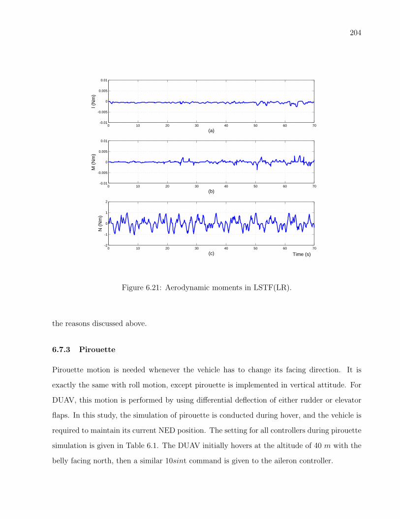
204

0 10 20 30 40 50 60 70-0.01

-0.005

0

0.005

0.01

l (N

m)

(a)

0 10 20 30 40 50 60 70-0.01

-0.005

0

0.005

0.01

M (N

m)

(b)

0 10 20 30 40 50 60 70-2

-1

0

1

2

N (N

m)

(c) Time (s)

Figure 6.21: Aerodynamic moments in LSTF(LR).

the reasons discussed above.

6.7.3 Pirouette

Pirouette motion is needed whenever the vehicle has to change its facing direction. It is

exactly the same with roll motion, except pirouette is implemented in vertical attitude. For

DUAV, this motion is performed by using differential deflection of either rudder or elevator

flaps. In this study, the simulation of pirouette is conducted during hover, and the vehicle is

required to maintain its current NED position. The setting for all controllers during pirouette

simulation is given in Table 6.1. The DUAV initially hovers at the altitude of 40 m with the

belly facing north, then a similar 10sint command is given to the aileron controller.

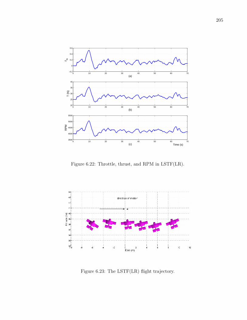
205

0 10 20 30 40 50 60 70-0.2

0

0.2

0.4

0.6

δ th

(a)

0 10 20 30 40 50 60 7020

25

30

35

40

T (N

)

(b)

0 10 20 30 40 50 60 703500

4000

4500

5000

5500

RPM

(c) Time (s)

Figure 6.22: Throttle, thrust, and RPM in LSTF(LR).

Figure 6.23: The LSTF(LR) flight trajectory.

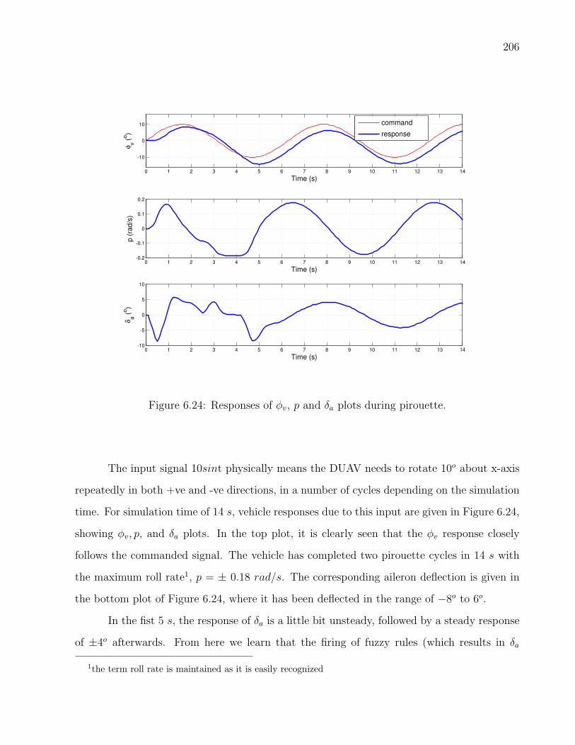
206

0 1 2 3 4 5 6 7 8 9 10 11 12 13 14

-10

0

10φ

v (

o)

Time (s)

0 1 2 3 4 5 6 7 8 9 10 11 12 13 14-0.2

-0.1

0

0.1

0.2

p (

rad

/s)

Time (s)

0 1 2 3 4 5 6 7 8 9 10 11 12 13 14-10

-5

0

5

10

δa (

o)

Time (s)

command

response

Figure 6.24: Responses of φv, p and δa plots during pirouette.

The input signal 10sint physically means the DUAV needs to rotate 10o about x-axis

repeatedly in both +ve and -ve directions, in a number of cycles depending on the simulation

time. For simulation time of 14 s, vehicle responses due to this input are given in Figure 6.24,

showing φv, p, and δa plots. In the top plot, it is clearly seen that the φv response closely

follows the commanded signal. The vehicle has completed two pirouette cycles in 14 s with

the maximum roll rate1, p = ± 0.18 rad/s. The corresponding aileron deflection is given in

the bottom plot of Figure 6.24, where it has been deflected in the range of −8o to 6o.

In the fist 5 s, the response of δa is a little bit unsteady, followed by a steady response

of ±4o afterwards. From here we learn that the firing of fuzzy rules (which results in δa

1the term roll rate is maintained as it is easily recognized

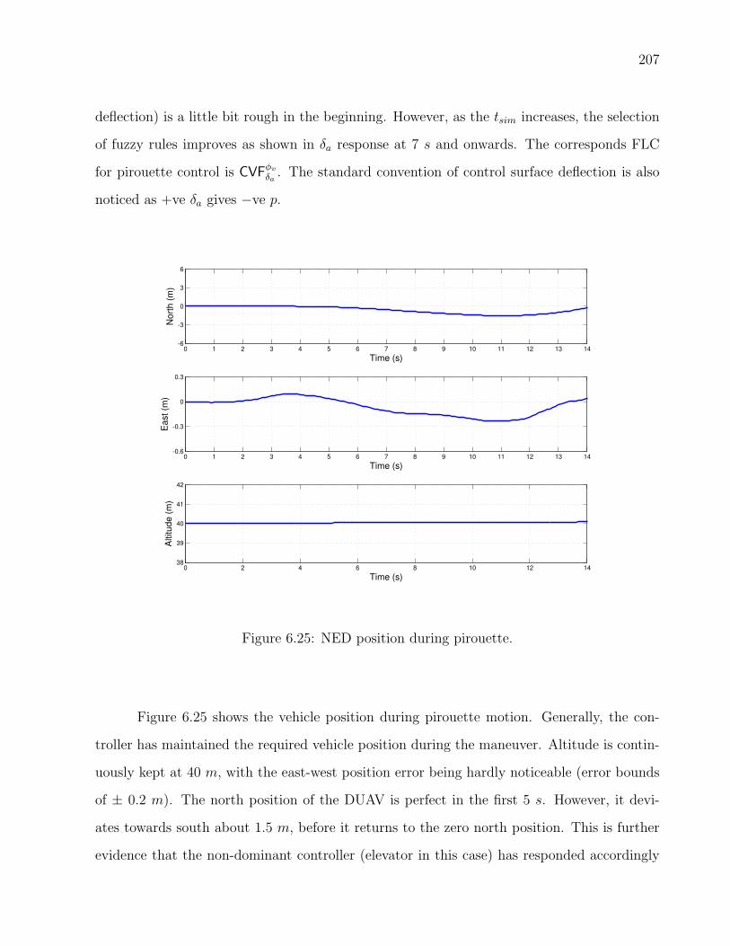
207

deflection) is a little bit rough in the beginning. However, as the tsim increases, the selection

of fuzzy rules improves as shown in δa response at 7 s and onwards. The corresponds FLC

for pirouette control is CVFφv

δa. The standard convention of control surface deflection is also

noticed as +ve δa gives −ve p.

0 1 2 3 4 5 6 7 8 9 10 11 12 13 14-6

-3

0

3

6

No

rth

(m

)

Time (s)

0 1 2 3 4 5 6 7 8 9 10 11 12 13 14-0.6

-0.3

0

0.3

Ea

st (m

)

Time (s)

0 2 4 6 8 10 12 1438

39

40

41

42

Altitu

de

(m

)

Time (s)

Figure 6.25: NED position during pirouette.

Figure 6.25 shows the vehicle position during pirouette motion. Generally, the con-

troller has maintained the required vehicle position during the maneuver. Altitude is contin-

uously kept at 40 m, with the east-west position error being hardly noticeable (error bounds

of ± 0.2 m). The north position of the DUAV is perfect in the first 5 s. However, it devi-

ates towards south about 1.5 m, before it returns to the zero north position. This is further

evidence that the non-dominant controller (elevator in this case) has responded accordingly

208

due to position error.

6.8 TRANSITION FLIGHT

This section presents the vehicle simulation results for two types of transition flights: vertical

to horizontal (VtoH) and horizontal to vertical (HtoV). Table 6.3 provides the commanded

signals in each flight simulation. During these short time maneuvers, the throttle is kept at

a constant setting. The zero settings for φc and ψc means the transition flight is set to be

implemented in xz plane of the vehicle body-axis. Scaling factors for transition flight FLCs

are given in Table 6.4.

Table 6.3: Command signals for transition flight simulation.

Flight Transition Mode VtoH HtoV

θinit(o) 90 0

Command θc(o) 0 90

Signal ψc(o) 0 0

φc(o) 0 0

Vinit(m/s) 40 30

6.8.1 Vertical to Horizontal Maneuver

The VtoH manoeuvre brings the DUAV from vertical to horizontal flight, heading north, thus

entering a high speed horizontal flight region. In this simulation section, the main concern

is only at the very moment of the body transition from vertical to horizontal which occurred

within relatively short seconds. The vehicle initially flies at the last point of vertical flight

with the velocity of 25 m/s, at the altitude of 100 m, and θ = 90o, before suddenly given

with a pitch angle command of θc = 0o.

As provided in Table 6.4, Set 1, Set 2, and Set 3 represent the variation of scaling

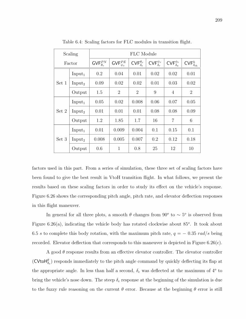
209

Table 6.4: Scaling factors for FLC modules in transition flight.

Scaling FLC Module

Factor GVFPNθvGVFPEψv

CVFθvδe

CVFψv

δrCVFφv

δaCVFhδth

Input1 0.2 0.04 0.01 0.02 0.02 0.01

Set 1 Input2 0.09 0.02 0.02 0.01 0.03 0.02

Output 1.5 2 2 9 4 2

Input1 0.05 0.02 0.008 0.06 0.07 0.05

Set 2 Input2 0.01 0.01 0.01 0.08 0.08 0.09

Output 1.2 1.85 1.7 16 7 6

Input1 0.01 0.009 0.004 0.1 0.15 0.1

Set 3 Input2 0.008 0.005 0.007 0.2 0.12 0.18

Output 0.6 1 0.8 25 12 10

factors used in this part. From a series of simulation, these three set of scaling factors have

been found to give the best result in VtoH transition flight. In what follows, we present the

results based on these scaling factors in order to study its effect on the vehicle’s response.

Figure 6.26 shows the corresponding pitch angle, pitch rate, and elevator deflection responses

in this flight maneuver.

In general for all three plots, a smooth θ changes from 90o to ∼ 5o is observed from

Figure 6.26(a), indicating the vehicle body has rotated clockwise about 85o. It took about

6.5 s to complete this body rotation, with the maximum pitch rate, q = − 0.35 rad/s being

recorded. Elevator deflection that corresponds to this maneuver is depicted in Figure 6.26(c).

A good θ response results from an effective elevator controller. The elevator controller

(CVtoHθδe) responds immediately to the pitch angle command by quickly deflecting its flap at

the appropriate angle. In less than half a second, δe was deflected at the maximum of 4o to

bring the vehicle’s nose down. The steep δe response at the beginning of the simulation is due

to the fuzzy rule reasoning on the current θ error. Because at the beginning θ error is still

210

0 0.5 1 1.5 2 2.5 3 3.5 4 4.5 5 5.5 6 6.5 7 7.5 880

15

30

45

60

75

90

100100

θ (

o)

(a)

0 0.5 1 1.5 2 2.5 3 3.5 4 4.5 5 5.5 6 6.5 7 7.5 88-0.4

-0.3

-0.2

-0.1

0

0.10.1

q (

rad

/s)

(b)

0 0.5 1 1.5 2 2.5 3 3.5 4 4.5 5 5.5 6 6.5 7 7.5 88-6

-4

-2

0

2

4

66

δe (

o)

Time (s)(c)

Set 1

Set 2

Set 3

Figure 6.26: Euler, pitch rate, and elevator deflection during VtoH.

huge, thus a big δe is also needed to reduce this error. In the vehicle responses in Figure 6.26,

the sign convention of elevator deflection can be seen: +ve δe gives −ve q, and vice versa.

By carefully examine all plots in Figure 6.26, we notice that set 1 scaling factors give

the best responses compared to the rest two sets. For θ, the blue plot (set 1) is almost reach

0o, where it indicates the vehicle is almost level. The green (set 2) terminated at a higher

θ, while the red plot (set 3) terminated at the most highest θ, at about 7o. The trend of

response is consistent in pitch rate and elevator plots as shown in Figure 6.26(b) and 6.26(c)

respectively. In Figure 6.26(b), we can observe the blue plot gives the most less pitch rate,

while in Figure 6.26(c), the blue plot shows the most less elevator deflection when compared

212

altitude gained of about 95 m.

For the north plot shown in Figure 6.27(b) , the use of set 2 and set 3 scaling factors

cause the vehicle to travel further to the north. Notice the purple plot in Figure 6.27(b)

that shows the east trajectory is maintained at zero throughout the simulation, where it

demonstrates that the transition flight has occurred exactly on the symmetrical xz body-axis

plane.

Since at the entry point of the maneuver, the forward velocity of the vehicle is con-

stantly decreases. This is due to the fact that the throttle setting is kept constant. At the

last point of vertical flight, the δth setting is “locked”, therefore the throttle maintains this

setting throughout the VtoH maneuver. Since the VtoH motion opposes the gravity, and no

additional thrust is given, we observe a decrease in the vehicle velocity from 25 m/s to 19

m/s as can be seen in Figure 6.27(c). Also note that there is a small variation in the velocity

decrement where the use of set 1 scaling factor causes the maximum velocity drop of 6 m/s.

Aerodynamic moments’ responses in the VtoH maneuver are given in Figure 6.28. We

can see from Figure 6.28(a) and 6.28(c) that both rolling and yawing moments are zero.

This again confirms the VtoH maneuver is carried out perfectly in the symmetrical xz plane.

Similar results are obtained for these moments irrespective of any scaling factor. Also note

there are some fluctuations on the responses, especially for yawing moment. This noise is due

the wind gust that was included in the simulation as described in Section 6.4.

The only useful moment in the transition flight is pitching. Note at the beginning

of the response in Figure 6.28(b) that the negative pitching moment causes the DUAV to

rotate clockwise from vertical orientation. Pitching moment from set 1 scaling factors is

slightly less when compared with the results from the other two sets scaling factors. This

demonstrates that less effort is needed by the UAV to complete the VtoH transition flight by

using appropriate scaling factors. The body’s rotation in VtoH maneuver can be thought to

be a similar case in normal level flight when the vehicle is given with -ve pitching moment, it

will pitch down.

213

0 0.5 1 1.5 2 2.5 3 3.5 4 4.5 5 5.5 6 6.5 77-3

-1.5

0

1.5

33x 10

-3

l (N

m)

Time (s)

0 0.5 1 1.5 2 2.5 3 3.5 4 4.5 5 5.5 6 6.5 77-0.2

-0.1

0

0.1

M (

Nm

)

Time (s)

0 0.5 1 1.5 2 2.5 3 3.5 4 4.5 5 5.5 6 6.5 77-1

-0.5

0

0.5

11x 10

-3

N (

Nm

)

Time (s)

Set 1

Set 2

Set 3

Figure 6.28: Aerodynamic moments during VtoH.

Results for VtoH transition flight in Figure 6.26 to Figure 6.28 show consistency where

responses from set 1 scaling factors are the most preferable. Observing these plots together

with the scaling factors given in Table 6.4, we can deduce several findings on the effect of

scaling factors. For GVFPNθvmodule, the scaling factors that are tested on the first input are

0.01, 0.05, and 0.2. It is clear from Table 6.4 that the most preferable vehicle’s response is

obtained through the biggest scaling factor of 0.2. Decreasing this scaling factor worsens the

result as can be seen in Figure 6.27(b) where the farther north position is recorded.

Similar trends are obtained for the second input and the output of GVFPNθvmodule,

where the results are improved by increasing the scaling factors. Data in Table 6.4 also

214

shows that by increasing all scaling factors for inputs and output for both GVFPEψvand CVFθv

δe

modules, better results are obtained. However, a contrary characteristic on the scaling factors’

settings are noticed in the rest three fuzzy modules CVFψv

δr, CVFφv

δa, and CVFhδth , where the

most preferable result are found by decreasing the scaling factors. Generally, considerable

effort has been devoted in the trial and error procedure before we finally arrived on the range

of scaling factors presented in Table 6.4.

Back to the maximum altitude gained in Figure 6.27(a), the fully rotated body that

occurred at PN ∼ 50 m can also be observed in the trajectory model plot in Figure 6.29.

The figure shows the snapshot of VtoH maneuver on the xz plane where at PN ∼ 50 m, it

shows the DUAV is already in the horizontal attitude.

Figure 6.29: The aircraft trajectory model of VtoH transition.

215

6.8.2 Horizontal to Vertical Maneuver

The reverse transition flight, HtoV, is an extreme pull-up maneuver to bring the DUAV back

to the vertical attitude. Similar to VtoH, the completion of the HtoV transition flight also

takes minimal time. Initially, the vehicle is flying at a steady, straight, and level flight with

forward velocity of 30 ms−1. Then, a pitch angle command for HtoV is given to the vehicle

controller, which is θc = 90o. Figure 6.30 shows the vehicle’s response in this flight: pitch

angle, pitch rate, and elevator deflection plots. The first plot shows how θ changes quickly

and smoothly from 0o to 80o in just 1.5 s, and later completes almost 90o rotation in another

1.5 s.

0 0.25 0.5 0.75 1 1.25 1.5 1.75 2 2.25 2.5 2.75 3 3.25 3.5 3.75 4-1

-0.5

0

0.5

1

1.5

q (

rad

/s)

Time (s)

0 0.25 0.5 0.75 1 1.25 1.5 1.75 2 2.25 2.5 2.75 3 3.25 3.5 3.75 4-20

-15

-10

-5

0

4

δe (

o)

Time (s)

0 0.25 0.5 0.75 1 1.25 1.5 1.75 2 2.25 2.5 2.75 3 3.25 3.5 3.75 40

25

50

75

100

θ (

o)

Time (s)

Figure 6.30: Pitch angle, pitch rate, and elevator deflection during HtoV.

This means the full body rotation from horizontal to vertical takes 3 s with the max-

imum attained pitch rate is 1.4 rad/s as shown in the middle plot. As the vehicle is very

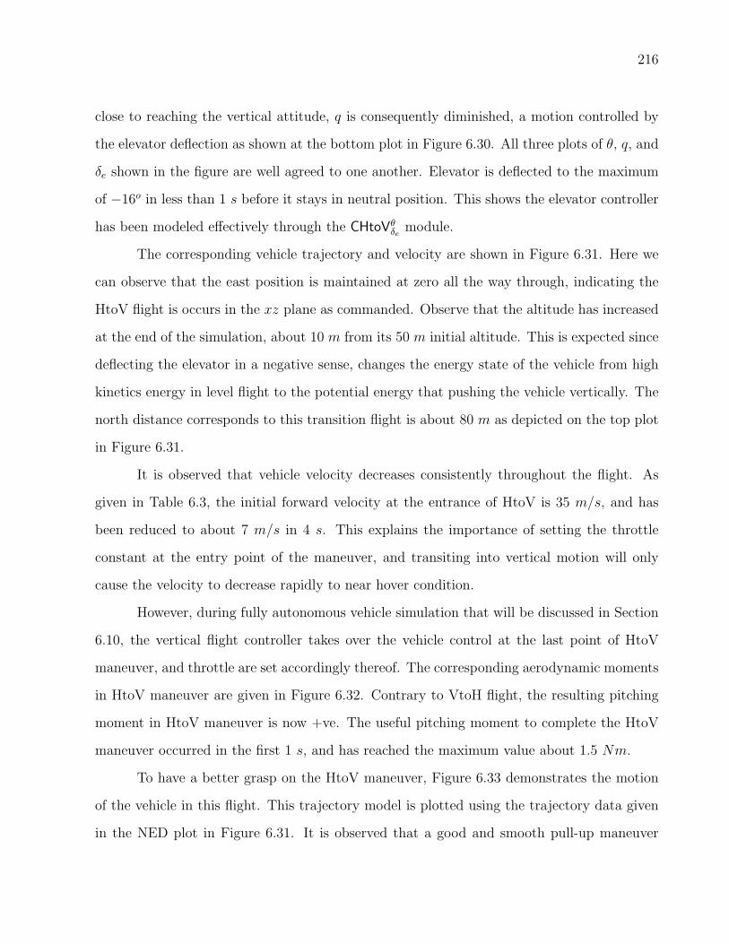
216

close to reaching the vertical attitude, q is consequently diminished, a motion controlled by

the elevator deflection as shown at the bottom plot in Figure 6.30. All three plots of θ, q, and

δe shown in the figure are well agreed to one another. Elevator is deflected to the maximum

of −16o in less than 1 s before it stays in neutral position. This shows the elevator controller

has been modeled effectively through the CHtoVθδe module.

The corresponding vehicle trajectory and velocity are shown in Figure 6.31. Here we

can observe that the east position is maintained at zero all the way through, indicating the

HtoV flight is occurs in the xz plane as commanded. Observe that the altitude has increased

at the end of the simulation, about 10 m from its 50 m initial altitude. This is expected since

deflecting the elevator in a negative sense, changes the energy state of the vehicle from high

kinetics energy in level flight to the potential energy that pushing the vehicle vertically. The

north distance corresponds to this transition flight is about 80 m as depicted on the top plot

in Figure 6.31.

It is observed that vehicle velocity decreases consistently throughout the flight. As

given in Table 6.3, the initial forward velocity at the entrance of HtoV is 35 m/s, and has

been reduced to about 7 m/s in 4 s. This explains the importance of setting the throttle

constant at the entry point of the maneuver, and transiting into vertical motion will only

cause the velocity to decrease rapidly to near hover condition.

However, during fully autonomous vehicle simulation that will be discussed in Section

6.10, the vertical flight controller takes over the vehicle control at the last point of HtoV

maneuver, and throttle are set accordingly thereof. The corresponding aerodynamic moments

in HtoV maneuver are given in Figure 6.32. Contrary to VtoH flight, the resulting pitching

moment in HtoV maneuver is now +ve. The useful pitching moment to complete the HtoV

maneuver occurred in the first 1 s, and has reached the maximum value about 1.5 Nm.

To have a better grasp on the HtoV maneuver, Figure 6.33 demonstrates the motion

of the vehicle in this flight. This trajectory model is plotted using the trajectory data given

in the NED plot in Figure 6.31. It is observed that a good and smooth pull-up maneuver

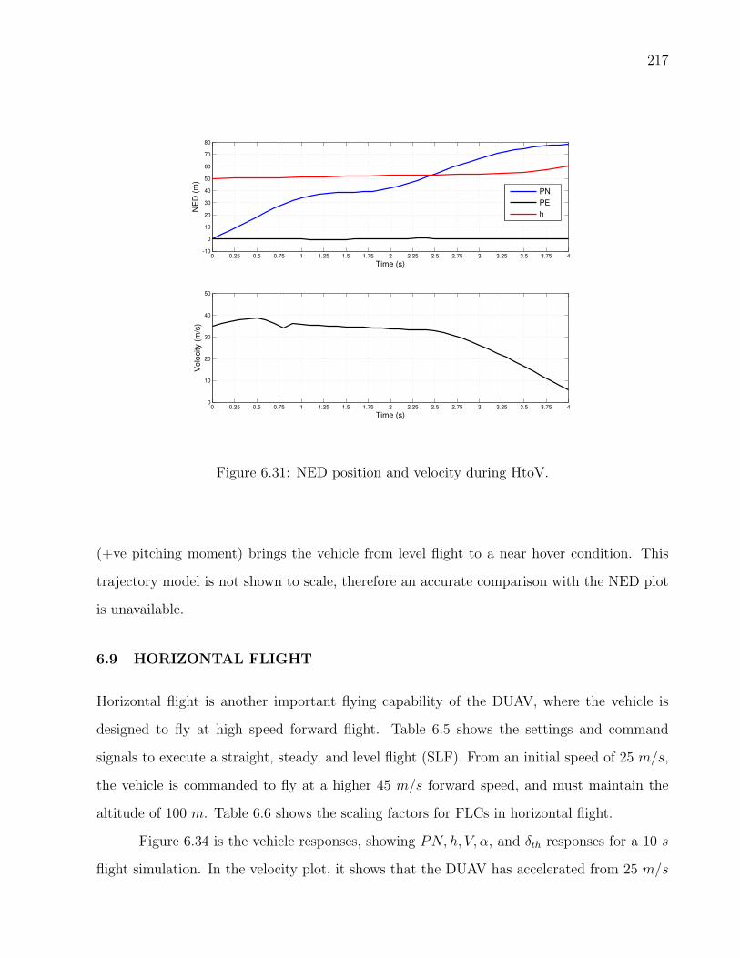
217

0 0.25 0.5 0.75 1 1.25 1.5 1.75 2 2.25 2.5 2.75 3 3.25 3.5 3.75 40

10

20

30

40

50

Ve

locity (

m/s

)

Time (s)

0 0.25 0.5 0.75 1 1.25 1.5 1.75 2 2.25 2.5 2.75 3 3.25 3.5 3.75 4-10

0

10

20

30

40

50

60

70

80

NE

D (

m)

Time (s)

PN

PE

h

Figure 6.31: NED position and velocity during HtoV.

(+ve pitching moment) brings the vehicle from level flight to a near hover condition. This

trajectory model is not shown to scale, therefore an accurate comparison with the NED plot

is unavailable.

6.9 HORIZONTAL FLIGHT

Horizontal flight is another important flying capability of the DUAV, where the vehicle is

designed to fly at high speed forward flight. Table 6.5 shows the settings and command

signals to execute a straight, steady, and level flight (SLF). From an initial speed of 25 m/s,

the vehicle is commanded to fly at a higher 45 m/s forward speed, and must maintain the

altitude of 100 m. Table 6.6 shows the scaling factors for FLCs in horizontal flight.

Figure 6.34 is the vehicle responses, showing PN, h, V, α, and δth responses for a 10 s

flight simulation. In the velocity plot, it shows that the DUAV has accelerated from 25 m/s

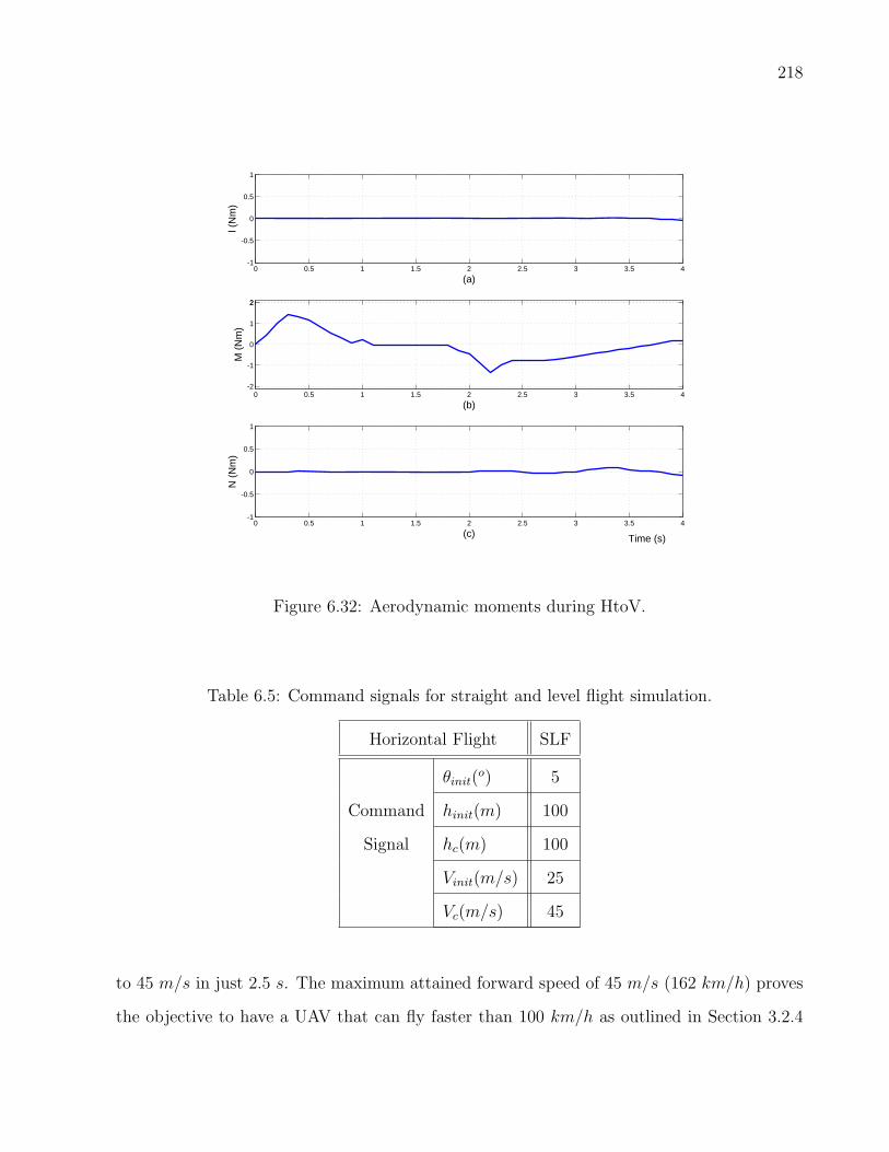
218

0 0.5 1 1.5 2 2.5 3 3.5 4-1

-0.5

0

0.5

1

l (N

m)

(a)

0 0.5 1 1.5 2 2.5 3 3.5 4-2

-1

0

1

22

M (N

m)

(b)

0 0.5 1 1.5 2 2.5 3 3.5 4-1

-0.5

0

0.5

1

N (N

m)

(c) Time (s)

Figure 6.32: Aerodynamic moments during HtoV.

Table 6.5: Command signals for straight and level flight simulation.

Horizontal Flight SLF

θinit(o) 5

Command hinit(m) 100

Signal hc(m) 100

Vinit(m/s) 25

Vc(m/s) 45

to 45 m/s in just 2.5 s. The maximum attained forward speed of 45 m/s (162 km/h) proves

the objective to have a UAV that can fly faster than 100 km/h as outlined in Section 3.2.4

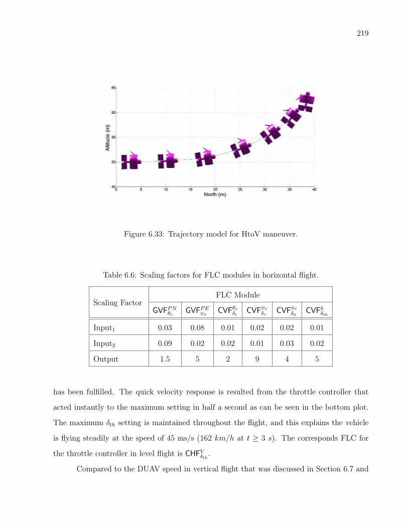
219

Figure 6.33: Trajectory model for HtoV maneuver.

Table 6.6: Scaling factors for FLC modules in horizontal flight.

Scaling FactorFLC Module

GVFPNθvGVFPEψv

CVFθvδe

CVFψv

δrCVFφv

δaCVFhδth

Input1 0.03 0.08 0.01 0.02 0.02 0.01

Input2 0.09 0.02 0.02 0.01 0.03 0.02

Output 1.5 5 2 9 4 5

has been fulfilled. The quick velocity response is resulted from the throttle controller that

acted instantly to the maximum setting in half a second as can be seen in the bottom plot.

The maximum δth setting is maintained throughout the flight, and this explains the vehicle

is flying steadily at the speed of 45 ms/s (162 km/h at t ≥ 3 s). The corresponds FLC for

the throttle controller in level flight is CHFVδth .

Compared to the DUAV speed in vertical flight that was discussed in Section 6.7 and

220

6.7.2, which is between 3 m/s to 8 m/s, the attainable forward speed in this SLF is hugely

different. Altitude is maintained at 100 m, although there was bit of jerking (< 0.5 m) at the

beginning of the simulation. We will discuss this altitude jerking later in this section. The

corresponds north flying distance is about 450 m as shown in the top plot of Figure 6.34.

Angle of attack plot also shows a consistent value of 5o, indicating a steady level flight is

achieved all the way through.

0 1 2 3 4 5 6 7 8 9 100

200

400

600

PN

(m

)

0 1 2 3 4 5 6 7 8 9 1099

99.5

100

100.5

101

h (

m)

0 1 2 3 4 5 6 7 8 9 1020

30

40

50

V (

m/s

)

0 1 2 3 4 5 6 7 8 9 100

2.5

5

7.5

10

α (

o)

0 1 2 3 4 5 6 7 8 9 100

0.5

1

1.5

δth

(o)

Time (s)

Figure 6.34: Position, altitude, velocity, angle of attack, and throttle setting during straightand level flight.

Figure 6.35 shows the corresponding vehicle responses of θ, q, and δe. It shows the 5o

pitch angle is maintained throughout, although there is minimal decrease (≤ 0.2o) towards

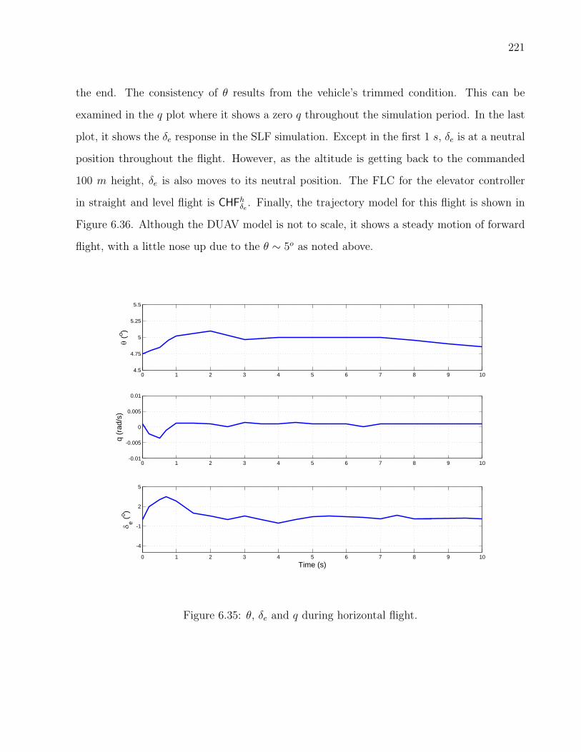
221

the end. The consistency of θ results from the vehicle’s trimmed condition. This can be

examined in the q plot where it shows a zero q throughout the simulation period. In the last

plot, it shows the δe response in the SLF simulation. Except in the first 1 s, δe is at a neutral

position throughout the flight. However, as the altitude is getting back to the commanded

100 m height, δe is also moves to its neutral position. The FLC for the elevator controller

in straight and level flight is CHFhδe . Finally, the trajectory model for this flight is shown in

Figure 6.36. Although the DUAV model is not to scale, it shows a steady motion of forward

flight, with a little nose up due to the θ ∼ 5o as noted above.

0 1 2 3 4 5 6 7 8 9 104.5

4.75

5

5.25

5.5

θ (o )

0 1 2 3 4 5 6 7 8 9 10

-4

-1

2

5

δ e (o )

Time (s)

0 1 2 3 4 5 6 7 8 9 10-0.01

-0.005

0

0.005

0.01

q (r

ad/s

)

Figure 6.35: θ, δe and q during horizontal flight.

222

Figure 6.36: Trajectory model for straight and level flight simulation.

6.9.1 Power Effect on Aerodynamic

A unique feature of the DUAV is it uses the slipstream dynamic pressure for using conventional

control surfaces placed behind the duct exit. The useful aerodynamic force generated over

these control surfaces is a function of slipstream dynamic pressure. Then the dynamic pressure

of the slipstream is a function of the power available. Clearly, different power available can be

expressed by different throttle settings. In this horizontal flight simulation, the effect of such

phenomenon is examined. Figure 6.37 shows several variables of interest which are useful to

observe the effect of power setting on the control surface aerodynamic.

The responses of dynamic pressure q, and lift, L to a linear increment of δth are recorded

for 0.5 s. Initially, the DUAV is in cruising flight before the throttle is suddenly increased

linearly from 50 % to 100 % settings. We can see as the power increases, the slipstream

dynamic pressure increases accordingly. Finally, we notice that the increase of slipstream

dynamic pressure causes more lift to be generated. The additional amount of lift generated

by the increment of 50 % power setting is about 15 % of the initial lift. This indicates that

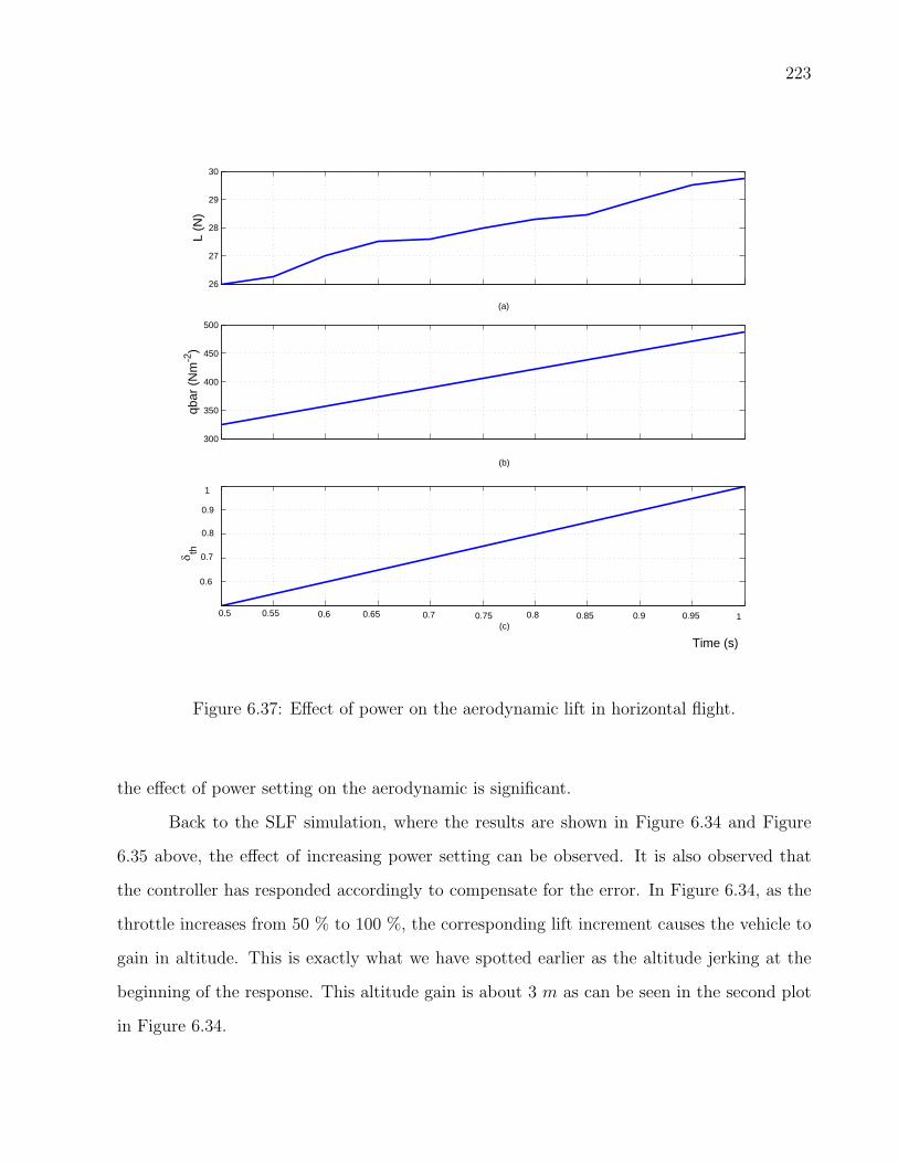
223

26

27

28

29

30

L (N

)

300

350

400

450

500

qbar

(Nm

-2)

0.5 0.55 0.6 0.65 0.7 0.75 0.8 0.85 0.9 0.95 1

0.6

0.7

0.8

0.9

1

δ th

Time (s)

(a)

(c)

(b)

Figure 6.37: Effect of power on the aerodynamic lift in horizontal flight.

the effect of power setting on the aerodynamic is significant.

Back to the SLF simulation, where the results are shown in Figure 6.34 and Figure

6.35 above, the effect of increasing power setting can be observed. It is also observed that

the controller has responded accordingly to compensate for the error. In Figure 6.34, as the

throttle increases from 50 % to 100 %, the corresponding lift increment causes the vehicle to

gain in altitude. This is exactly what we have spotted earlier as the altitude jerking at the

beginning of the response. This altitude gain is about 3 m as can be seen in the second plot

in Figure 6.34.

224

Since the objective in SLF is to maintain the altitude, this 3 m altitude gain is an

error. To correct this error, the FLC reacts immediately by causing the elevator to deflect

towards +ve side, thus causing the vehicle to pitch down, and subsequently the altitude is

reduced. This is the reason why we notice in Figure 6.35 the elevator is deflected positively

about 3o between 0.5 s to 1 s of the simulation time. The corresponding pitch rate and pitch

angle during this altitude error compensation can also be observed in Figure 6.35. As the

altitude is back to 100 m, no altitude error is detected, thus the controller is relaxed.

6.10 AUTONOMOUS MISSION

So far we have discussed numerous simulation results that were based on the individual flight

modes in the following order: vertical flight, transition flight, and horizontal flight. In this

section, we integrate all flight motions in a simulation module, to form an autonomous mission

for the DUAV. Although at this moment we are still not considering roll and bank motions

in the high speed lateral-directional flight segment, the autonomous mission can still be

implemented in the three-dimensional space because we have modeled the pirouette motion,

through which the vehicle can virtually point in any direction. This mission is conducted in

three-dimensional space by giving a series of commands, in chronological order, as shown in

Table 6.7.

A series of 14 steps flight commands are designed in the mission system, together

with their corresponding command signals and initial settings. Each flight command is quite

straightforward, for example in step 6, the vehicle needs to hover for 5 s. The way command

signals and initial settings are given, are exactly the same with what we have discussed in

their individual simulation, except their values may differ. Note that for hover and SLF, the

given tsim is a relative measurement from the current flight simulation time. The NR (not

relevant) notation is easily understood, for example the use of velocity command (Vc) is only

for horizontal flight.

The DUAV initial attitude as mentioned in Section 6.7 is maintained: θvinit= φvinit

=

225

Table 6.7: Flight commands and settings for an autonomous mission.

Flight Command (FC)

Command Signal

& Initial Setting

hinit (m) hc (m) PNc (m) PEc (m) Vc (m/s)

1. Ascend to 50 m 0 50 0 0 NR

2. Execute VtoH (θc = 0o) NR NR NR 0 NR

3. Execute SLF for tsim = 3 s last h of 2 last h of 2 NR NR 45

4. Execute HtoV (θc = 90o) NR NR NR 0 NR

5. Hover for tsim = 5 s last h of 4 last h of 4 0 0 NR

6. Pirouette (φvc = 90o) last h of 5 last h of 5 0 0 NR

7. Descend to 5 m last h of 6 50 0 0 NR

8. Execute 50 m LSTF(FB) last h of 7 last h of 7 50 0 NR

9. Pirouette (φvc = 90o) last h of 8 last h of 8 0 0 NR

10. Ascend to 50 m last h of 9 50 0 0 NR

11. Execute VtoH (θc = 0o) NR NR NR 0 NR

12. Execute SLF tsim = 3 s last h of 11 last h of 10 NR NR 45

13. Execute HtoV (θc = 0o) NR NR NR 0 NR

14. Descend to the ground last h of 13 0 0 0 NR

0o (not shown in Table 6.7). In Section 5.7, we generally described how Stateflow is used for

controller’s transitions in an autonomous mission on the longitudinal plane. Then, in Section

6.5, the actual implementation of Stateflow is shown in the Simulink R© environment. Now,

we extend the use of Stateflow for the same purposes, but applies to a fully autonomous

mission in three-dimensional flying space. To do this, the flight mission given in Table 6.7 is

reinterpreted in a form that can be understood by the Stateflow toolbox.

This is as given in Table 6.8, where it contains all the information needed by the

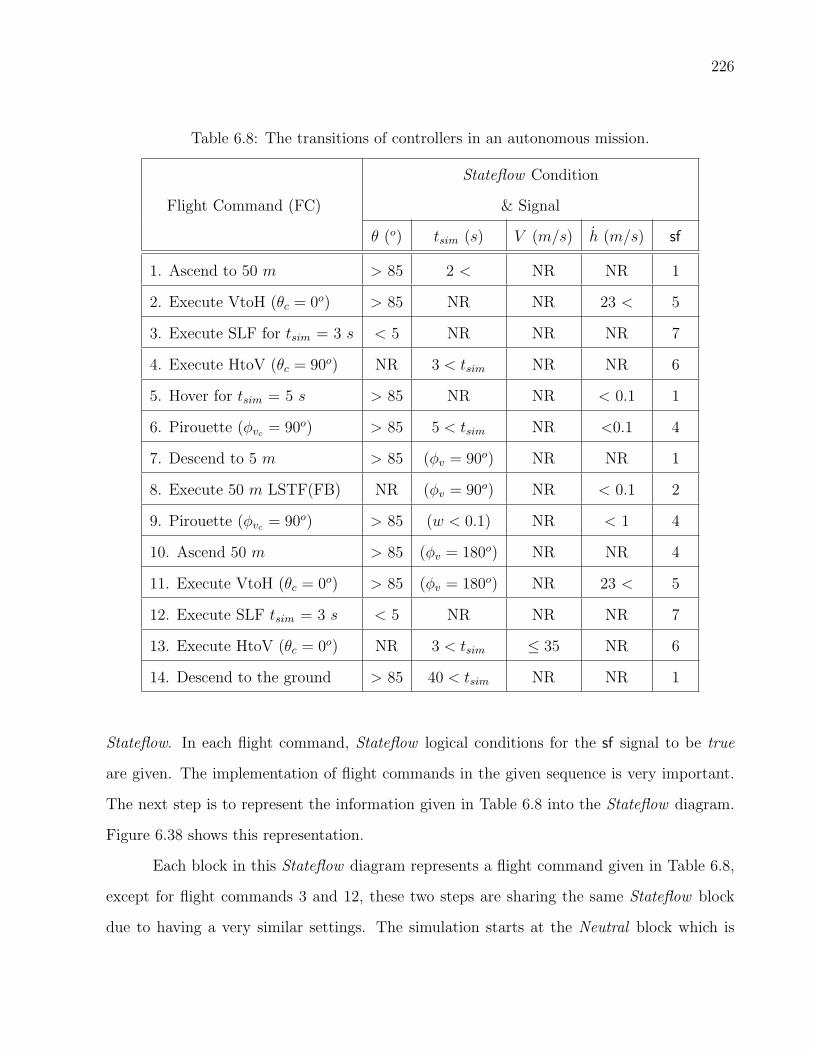
226

Table 6.8: The transitions of controllers in an autonomous mission.

Flight Command (FC)

Stateflow Condition

& Signal

θ (o) tsim (s) V (m/s) h (m/s) sf

1. Ascend to 50 m > 85 2 < NR NR 1

2. Execute VtoH (θc = 0o) > 85 NR NR 23 < 5

3. Execute SLF for tsim = 3 s < 5 NR NR NR 7

4. Execute HtoV (θc = 90o) NR 3 < tsim NR NR 6

5. Hover for tsim = 5 s > 85 NR NR < 0.1 1

6. Pirouette (φvc = 90o) > 85 5 < tsim NR <0.1 4

7. Descend to 5 m > 85 (φv = 90o) NR NR 1

8. Execute 50 m LSTF(FB) NR (φv = 90o) NR < 0.1 2

9. Pirouette (φvc = 90o) > 85 (w < 0.1) NR < 1 4

10. Ascend 50 m > 85 (φv = 180o) NR NR 4

11. Execute VtoH (θc = 0o) > 85 (φv = 180o) NR 23 < 5

12. Execute SLF tsim = 3 s < 5 NR NR NR 7

13. Execute HtoV (θc = 0o) NR 3 < tsim ≤ 35 NR 6

14. Descend to the ground > 85 40 < tsim NR NR 1

Stateflow. In each flight command, Stateflow logical conditions for the sf signal to be true

are given. The implementation of flight commands in the given sequence is very important.

The next step is to represent the information given in Table 6.8 into the Stateflow diagram.

Figure 6.38 shows this representation.

Each block in this Stateflow diagram represents a flight command given in Table 6.8,

except for flight commands 3 and 12, these two steps are sharing the same Stateflow block

due to having a very similar settings. The simulation starts at the Neutral block which is

227

indicated by a disconnected arrow, moving to the Ascend block, continuing to the right, and

it goes on by connecting arrows. Finally, the simulation ends at the same starting block when

h = 0 m.

During the simulation, each arrow is highlighted in the corresponding sequence, which

enables the user to know the current location of the Stateflow signal in real-time. Similar

to the settings that were discussed in Section 5.7, several restrictions are in placed such as θ

has to reach 85o and vertical speed has to be greater than 23 m/s before the VtoH can be

commanded. The rest of the Stateflow conditions are easily recognized through the notation

placed on each arrow.

Figure 6.39 shows the vehicle trajectory in this autonomous mission that lasts about

1 minute. A lot of comparison can be made between these NED plots with the information

DU_auto_sf/signal_flow3D

Ascend

en:sf=1;

en:hc=h+50;

SLF

en:sf=7;

Ascend

en:sf=1;

en:hc=50;

VtoH

en:sfn=5;

Pirouette

en:sf=4

HtoV

en:sf=6;

Hover

en:sf=1

en:hc=50;

Neutral

Pirouette

en:sf=4

Descend

en:sf=1;

en:hc=45;

LSTF(FB)

en:sf=2;

Descend

en:sf=1;

en:hc=0;

[(tsim3>3)&&(V<=35)]

[theta<5]

[(hdot>=23)&&(theta>=85)]

[phiV~=180]

[hdot >=23]

[(tsim1>3)&&(V<=35)]

[tsim>=2]

[tsim2>5]

[(hdot<=0.1)&&(theta>=85)]

[(theta>=85)&& tsim>40)][h=0][phiV~=90]

[w<0.1]

[hdot <0.1]

Figure 6.38: A Stateflow diagram for an autonomous flight mission in 3D space.

228

0 5 10 15 20 25 30 35 40 45 50 55 60-50

0

50

100

150

200

No

rth

(m

)

Time (s)

0 5 10 15 20 25 30 35 40 45 50 55 60-60

-40

-20

0

20

Ea

st (m

)

Time (s)

0 5 10 15 20 25 30 35 40 45 50 55 600

10

20

30

40

50

60

Altitu

de

(m

)

Time (s)

Figure 6.39: NED plot in the autonomous mission.

given in Table 6.7 and 6.8, step by step, in order to examine the vehicle responses on each

flight command. Take a look at the altitude plot in Figure 6.39, where it shows four peaks,

each at t ∼ 10 s, 21 s, 41 s, and 50 s. These peaks represent the highest altitude gained

during four transition maneuvers as given by FC2, FC4, FC11, and FC13 respectively. There

is consistency in these responses in terms of time taken to complete the maneuver and the

maximum reached altitude.

However, both VtoH at t ∼ 10 s and 41 s reach lower altitudes than it has in HtoV.

This is because the vehicle velocity prior to the VtoH is not as high as in HtoV. Lower velocity

means lower energy, thus causing lower gained altitude (less potential energy). The east plot

shows a good response with only a little oscillation (which means little error) throughout

211

to others.

0 0.5 1 1.5 2 2.5 3 3.5 4 4.5 5 5.5 6 6.5 77100

125

150

175

200200

Altitu

de

(m

)

(a)

0 0.5 1 1.5 2 2.5 3 3.5 4 4.5 5 5.5 6 6.5 719

20

21

22

23

24

25

Ve

locity (

m/s

)

Time (s)(c)

0 0.5 1 1.5 2 2.5 3 3.5 4 4.5 5 5.5 6 6.5 77-25

0

25

50

75

100100

No

rth

& E

ast (m

)

(b)

Set 1

Set 2

Set 3

East

Figure 6.27: Altitude, north and east position, and velocity during VtoH.

Figure 6.27 shows the vehicle trajectory and vehicle velocity during the VtoH maneu-

ver. By comparing θ plot in Figure 6.26(a) with the set 1 north plot in Figure 6.27(b), the

6.5 s used to complete the VtoH has caused the vehicle to fly about 75 m to the north. The

corresponding altitude in this situation is shown in Figure 6.27(a) with the maximum of 175

m is recorded. Remember that the vehicle is initially flown at the altitude of 100 m prior to

the VtoH maneuver, so this means the undesirable altitude gained in this case is 75 m. There

is a very little difference (1 m ∼ 5m) in the altitude gained between set 1 and set 2 plots as

can be seen in Figure 6.27(a). However, the use of set 3 scaling factor causes a significant

229

the flight. Here, the inclined plot shows the vehicle is flying to the west in LSTF(FB) mode

corresponds to the FC8 in Table 6.8.

In the north plot, the vehicle has flown to the farthest distance at about 155 m. The

“plateau” region indicates the LSTF(FB) flying mode with HtoV (FC4) and VtoH (FC11)

included at the start (t ∼ 17 s) and end point (t ∼ 38 s) respectively. On the other hand, the

“ground” region on the left side represents ascend (FC1) and VtoH (FC2), while the region

on the right side represents HtoV (FC13) and descend (FC14). Two steep regions shown in

the north plot are the moment when the DUAV is flying in SLF mode towards north (FC3)

and its return flight (FC12).

0 5 10 15 20 25 30 35 40 45 50 55 60-50

0

50

100

150

200

φ (

o)

Time (s)

0 5 10 15 20 25 30 35 40 45 50 55 60-50

0

50

100

150

200

θ (

o)

Time (s)

0 5 10 15 20 25 30 35 40 45 50 55 60-100

-75

-50

-25

0

ψ (

o)

Time (s)

Figure 6.40: Euler angles responses in the autonomous mission.

The responses of Euler angles in this flight simulation are shown in Figure 6.40. In the

230

same manner, we can examine each section in φ, θ, and ψ plots, then find the corresponding

flight trajectory given in Figure 6.39, and simultaneously check the flight command in Table

6.8 that corresponds to it. At anytime during the flight, the vehicle orientation is determined

by applying three Euler rotations as discussed in Section 4.4. Now, let’s examine Euler angles

responses at 25 s ≤ t35 s. To examine the vehicle attitude at this time range, follow the

procedure outlined in Section 4.4: first apply ψ ∼ −90o rotation, then θ ∼ 70o rotation, and

finally φ = 0o rotation. The final orientation represents the corresponding vehicle attitude,

which is exactly the vehicle attitude during LSTF(FB) to the west (FC8).

Finally, let us observe the vehicle trajectory model shown in Figure 6.41 that was

generated based on the data given in Figure 6.39. It reveals the actual motion of the DUAV

in this fully autonomous flight mission. Again, we can examine this motion plot with the

corresponding flight commands and flight responses given in Table 6.8 and in the last two

figures respectively. The flight mission can be thought as a 3D ’L’ maneuver that starts at

NED(0,0,0) and ends at NED(0, ∼ 50, 0). Note that the DUAV’s antenna is very useful in

checking the vehicle orientation at anytime during the flight. Although the DUAV motion

models shown in the figure are not to scale, it is very helpful in analyzing the 3D vehicle

trajectory, because it is rather hard to imagine a 3D motion from 2D plots.

6.11 SUMMARY

The essential objective of the research was answered in this chapter. Many vehicle simulation

results have proven that the proposed intelligent controller was successfully implemented on

the ducted-fan UAV. It was shown that this newly designed ducted-fan UAV was able to

perform various functional flights in vertical, transition, and horizontal modes. Furthermore,

the intelligent fuzzy logic controller has successfully controlled the vehicle even in the pres-

ence of wind disturbances. Results in terms of Euler angles, vehicle’s velocity, and control

surface deflections have shown a degree of reasonable stability was maintained throughout

the flight. The power effect on the lift was examined, and the corresponding FLC was proven

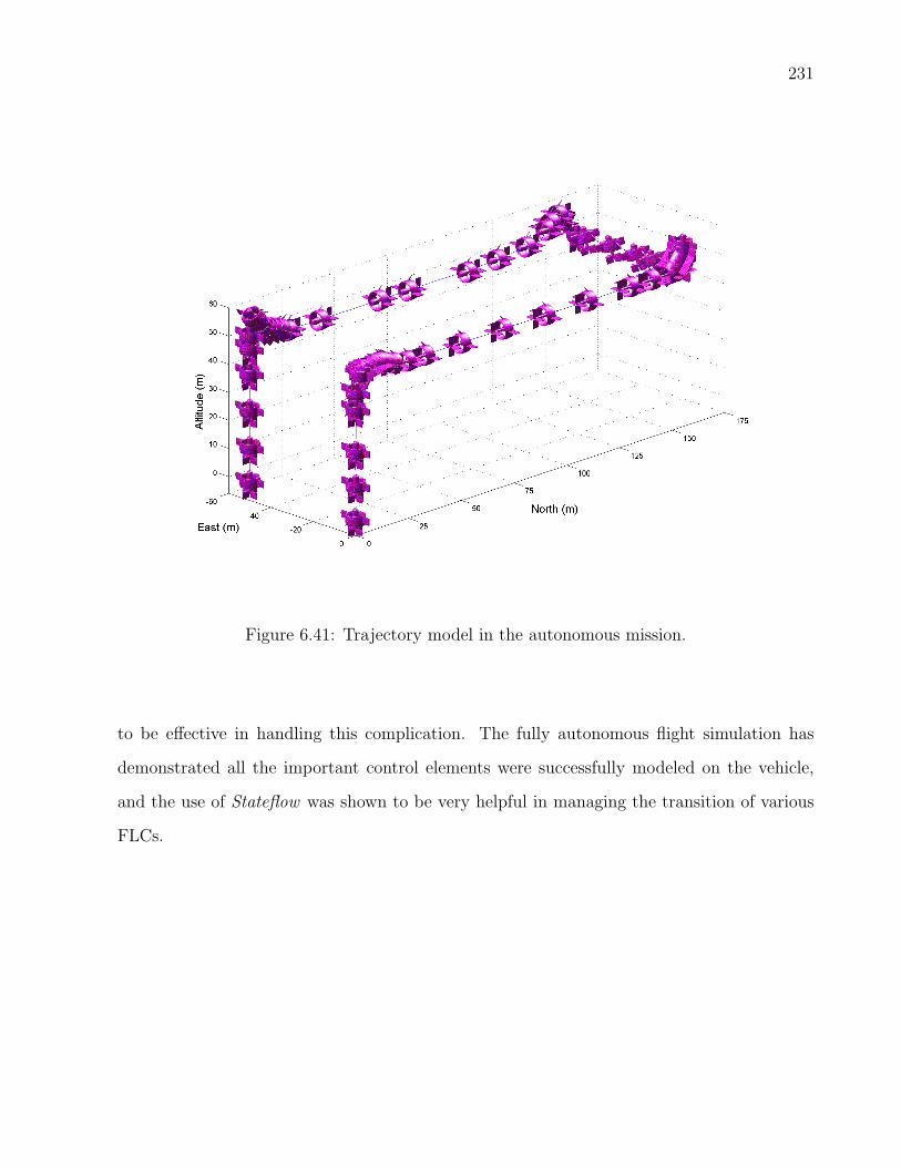
231

Figure 6.41: Trajectory model in the autonomous mission.

to be effective in handling this complication. The fully autonomous flight simulation has

demonstrated all the important control elements were successfully modeled on the vehicle,

and the use of Stateflow was shown to be very helpful in managing the transition of various

FLCs.

232

Chapter 7

THESIS CONTRIBUTIONS

Contributions to the body of knowledge that are made through this study are presented in

this chapter. Several implications to the current control approach are also highlighted. The

thesis contributions can be categorized into two aspects: control system design and UAV

design configuration.

7.1 CONTROL SYSTEM DESIGN

1. Autonomous Control: A fuzzy logic controller was successfully designed, developed,

and tested to control a ducted-fan UAV. It was proved in Section 6.10 that this con-

troller has shown good performance in controlling the vehicle, fully autonomous in a

three-dimensional flight mission. The vehicle was flying very closely to the commanded

trajectory and the changes of various FLC for different flight modes was successfully

managed by the Stateflow. This is the answer to the hypothesis highlighted in the

problem statement in Section 1.2, as to whether a fuzzy logic controller could perform

similar to a pilot.

This indicates the use of linguistic variables that represents the vehicle’s states, together

with the fuzzy rules are able to function properly in producing appropriate control laws

in various flight conditions. The use of linguistic variables replicates how a pilot makes

decisions. The achievement of autonomous control in various basic functional flights was

outlined in Section 6.7.1 to 6.9. Since all FLCs use triangular membership functions,

it means the use of this membership function type is sufficient to ensure considerably

good vehicle responses.

233

2. Stable flight: Without analyzing the vehicle’s stability, performance, and trim settings

prior to the controlled simulation, the use of FLC is still guarantees a stable flight.

The stable and trajectory-following flights of the DUAV can be seen in many NED

plots presented in Chapter 6. Note that these flight simulations are conducted in the

presence of wind disturbance. Prior to the controlled simulation using FLC, the degree

of static and dynamic stability of the vehicle is not known. Although a detailed stability

analysis based on the vehicle responses is not included in the scope of study, in general,

it is accepted that in any flight simulation (Section 6.7.1 to 6.10), a stable flight is

maintained.

This implicates that by using fuzzy logic controller in the simulation analysis, it is not

necessary to know the details of vehicle stability, performance, and trim settings in

advance, as along as the basic knowledge of the vehicle is known. The basic knowledge

of the vehicle here means the basic geometric, aerodynamic and propulsive data that are

sufficient for use in the modeling and simulation as given in Chapter 3. An important

point to note is that the FLC controls the vehicle in a totally different manner from

the conventional methods. When using FLC, the system does not need to be linearized

because it can deal with nonlinearities. As such, the linear analysis of the controller is

not applicable.

3. Simple control technique: Fuzzy logic is known as a simple, fast to develop, and less

mathematical technique that is based on human reasoning towards problems. Although

comparison of multiple control techniques is not in the scope of study, from the literature

it can generally be said that the development of fuzzy logic controller is quite simple and

fast. Fuzzy logic controller is simple in the sense that it can be developed heuristically

based on expert knowledge on the system.

In the case when expert knowledge is not available, knowledge of the system can be

determined through the first principle, which is to conduct modeling and simulation on

the system dynamics. These are among the things that were discussed in Chapter 5.

234

All these steps could be done without having too much analytical or numerical analysis.

Therefore, this thesis has proved that a simple fuzzy logic controller has resulted in

a reliable and effective method in controlling a highly nonlinear ducted-fan UAV. The

simple, fast to develop, and less mathematical jargon means it is able to reduce resources

such as cost, time, and computational effort.

7.2 UAV DESIGN CONFIGURATION

1. Design feasibility: The configuration of the DUAV presents a novelty for a small,

the VTOL type, and the ducted-fan UAV class. At this preliminary stage, it has been

shown that the UAV configuration has a reasonable degree of feasibility as discussed in

Section 3.1. It also has been shown that it was feasible to combine several important

design elements from rotorcraft, ducted-fan, and fixed-wing aircraft. Based on the

preliminary estimation of the vehicle aerodynamic in Section 3.3 and the study of the

effect of power setting on the aerodynamic in Section 6.9.1, this new UAV configuration

can have reasonable flight performance in both vertical and horizontal flights.

We have proved that this vehicle can technically fly and be controlled. Simulation results

in Chapter 6 show the vehicle is able to perform various kinds of flight maneuvers. The

concept of transition flights between vertical and horizontal modes is achievable. Also,

by using intelligent fuzzy logic controller, good vehicle control has been achieved, as

shown by simulation results in Chapter 6.

2. Vehicle capabilities: The aim to design a UAV that have several important capa-

bilities as highlighted in Section 2.3 have been achieved. In this newly designed UAV,

elements and capabilities of VTOL and UAV have been put together, which resulted in

a vehicle that is compact, ducted-fan type, and able to perform high speed horizontal

flight. The idea of putting together these characteristics on a new configuration is to

have a better UAV which can resolve many problems encountered by existing ducted-

UAVs. These three elements are crucial for any UAV to successfully perform flight

235

missions that are highlighted in Sections 1.2, 3.2.4, and 2.3. Since the DUAV has these

characteristics, this vehicle has the potential to fulfill all those missions effectively.

236

Chapter 8

CONCLUSION

An automatic controller based on fuzzy logic has been developed and successfully

implemented on a novel ducted-fan UAV configuration. Chapter 1 introduces the rationale of

carrying out the research relating to small ducted-fan UAV and the use of fuzzy logic approach

for its controller. Then, the problem statement of the thesis is clearly defined, followed by

the description of the scope and limitations of the research. In Chapter 2, the foundations of

research are presented in the forms of literature review and theoretical background. Here, the

discussion starts with the general needs for UAVs to have VTOL capability, we then narrow

down to various specific flight missions where a VTOL, small ducted-fan UAV is crucially

required.

We present several conventional approaches that are adopted for autonomous control

on existing ducted-fan UAVs. Some advantages and disadvantages of these control approaches

are highlighted. Due to the complex and high nonlinearities involved in the aerodynamic and

control of the ducted-fan UAV, the potential of using intelligent control approach for this

type of vehicle is emphasized. Specifically, we highlight, justify, and recommend the use of

fuzzy logic controller for the ducted-fan UAV which replicates how a pilot makes decisions,

or human reasoning in general. A thorough, but brief theoretical view on fuzzy logic is

presented. It includes the concept, foundations, characteristics, and steps to develop fuzzy

logic controller.

Chapter 3 reveals a new ducted-fan UAV configuration being developed at RMIT

University, where the author is one of the researchers who was working on this vehicle.

Several basic design elements of this vehicle, referred as the DUAV are provided such as the

vehicle concept, geometrical layout, and mass and inertia properties. The specialty of this

237

newly design UAV together with the potential flight missions are also presented. In this

chapter, a moderate but adequate analysis of the aerodynamic and propulsion of the vehicle

are presented. It discuss several aerodynamic considerations of the proposed ducted-fan UAV,

and estimation of some basic data for vehicle the simulation.

The dynamics modeling of the DUAV is developed and presented in Chapter 4. This

chapter explains the axis systems used, equations of motion, attitude representation methods,

transformation between axes, kinematics, navigational equations, and the method used to

solve the vehicle dynamics problem. Here, we derived six degrees of freedom equations of

motion for the DUAV that based on the rigid body aircraft and non-rotating earth-axis.

Because the DUAV spends considerable time in vertical flight, it is fitting to introduce

a new set of Euler angles, namely vertical Euler angles in order to define the vehicle attitude

in the vertical orientation. Transformations between normal Euler and vertical Euler can be

done as required. Transformation matrices between axes are derived, because to solve the

vehicle dynamics, it is essential to have some variables transformed to another axis such as

from body-axis to earth-axis.

Chapter 5 presents the central element of the study which is the development of fuzzy

logic controller for the DUAV. A detailed discussion on various flight modes of the DUAV is

provided, which are the vertical flight, the transition flight, and the horizontal flight. The

approach taken in developing an autonomous flight controller for the DUAV is clearly defined.

The structure of fuzzy logic controller is a feedback control system with two loops: guidance

and control loops. In relation to various flight modes involve in the DUAV flight, the control

approach is to develop a series of FLCs in modular forms based on these flight modes.

The concept of dominant controller is introduced where it explains in any flight mode,

there must be a main (dominant) controller that control the current flight motion. Then,

the properties of fuzzy logic controller are presented. Here, the common and uncommon

fuzzy properties for all FLCs are highlighted. The rest of materials in this chapter is the

modular development of the FLC for each flight mode. Since we have a number of FLCs

238

that are classified based on flight modes, Stateflow toolbox is the method used to manage the

transitions between FLCs. This is very useful for any flight that has several flight modes, and

especially important for fully autonomous flight in the three-dimensional coordinates frame.

The most important research findings which are the controlled vehicle simulation re-

sults are presented and discussed in Chapter 6. Simulation settings are highlighted, and a

wind disturbance model that was imposed in the simulation model is described. It begins

with discussion of the individual flight simulation results, where vehicle responses due to com-

manded input are observed and discussed. The individual flight simulation can be divided

into three flight modes: vertical flight, transition flight, and horizontal flight. In these flight

modes, there is further discussion on the results of flight variations. A discussion on the

effect of power setting on the vehicle aerodynamic, and the response of the FLC towards this

phenomenon were also presented in Section 6.9.1.

The final section presents simulation results of a fully autonomous flight mission in 3D

coordinate frame. Here, a flight command module is given for the vehicle to perform a fully

autonomous flight mission. The mission needs the vehicle to fly in 3D space by combining all

individual flight modes. The use of Stateflow toolbox is demonstrated in managing the change

of various kind of FLCs. At a particular time, Stateflow must ensure that the dominant FLC is

the authoritative controller. In short, all simulation results have shown a good vehicle response

and the DUAV was proven in a stable flight at all times, which indicates the developed fuzzy

logic controller has given good performance.

Chapter 7 summarizes the main contributions made in this thesis which can be classi-

fied either in the control system design part or in the UAV design configuration part. Finally,

this chapter concludes everything that is presented in this thesis, with several future works

related to this research being recommended, and publications related to this study are listed.

239

8.1 RECOMMENDED FUTURE WORKS

This thesis has presented a comprehensive preliminary study on a new design ducted-fan

VTOL UAV including design configuration, aerodynamic data estimation, fuzzy logic con-

troller, and flight simulation. It serves an important step towards the realization of building

and testing the actual UAV. To achieve this goal, there will be several recommended future

works related to this study that are as follows:

1. Vehicle model: Develop a more accurate vehicle aerodynamic data that covers the

fully six degrees of freedom flight envelope. Also to estimate uncertainties in the aero-

dynamic model. This can be done through a series of CFD simulations and wind tunnel

tests. The propulsion part should also be modeled towards a more realistic data based

on the available electric d.c motors.

2. Design details: Develop a details design configuration of the vehicle that shows all

the necessary steps and elements in the aircraft design.

3. Controller optimization: The fuzzy logic controller can be optimized in several ways.

Specifically in this study, the tuning of scaling gains is quite laborious and presents good

element for optimization.

4. Simulation Enhancement: The simulation should be made more realistic by includ-

ing details models for sensors and actuators. Also need to include discrete signals in

sampling periods and noise filtering in the simulation model.

5. Build a demonstrator: A proof-of-concept ducted-fan UAV demonstrator should be

built, with all necessary softwares and hardware are incorporated.

6. Flight Test: The proposed controller should installed on the onboard controller. Flight

data should be realistically given by various onboard sensors. Then a series of flight

tests should be conducted by using manual, semi autonomous, and fully autonomous

control, and will be monitored from a ground control station.

240

PUBLICATIONS

1. Zamri O., Bil C., and Hill R., “UAV Hovering Control Using Intelligent Fuzzy Tech-

nique”, Proceedings of the 3rd International Conference on Artificial Intelligence in

Engineering & Technology, Kota Kinabalu, November 2006.

2. Zamri O., Bil C., and Hill R., “Aerodynamic Characteristics of a Mini VTOL Ducted

Fan UAV”, AIAC12 Congress: 2nd Australasian Unmanned Air Vehicles Conference,

Melbourne, March 2007.

3. Zamri O., Bil C., and Hill R., “The Application of Fuzzy Logic on Transition Maneuver

Control of a New Ducted-Fan VTOL UAV Configuration”, IEEE 2nd Proceedings of

Innovative Computing, Information and Control, Kumamoto, September 2007.

4. Zamri O., Bil C., and Hill R., “The Development of A New VTOL UAV Configuration

For Law Enforcement”, 1st International Conference on Mechanical and Manufacturing

Engineering, Johor Bahru, May 2008.

241

REFERENCES

[1] European Commission Enterprise and Industry Directorate-General. “Study Analysing

The Current Activities in The Field of UAV”. Frost and Sullivan, Tech. Rep

ENTR/2007/065, 2007.

[2] K.C. Wong. (2009, June), “Aerospace Industry Opportunities in Australia : Un-

manned Aerial Vehicles - Are They Ready This Time? Are We?” [Online]., Available :

http://www.aeromech.usyd.edu.au/wwwdocs/UAV RAeS prez 26Nov97.PDF.

[3] Michael A.Turbe Eric N.Johnson. “Modeling, Control, and Flight Testing of a Small

Ducted-Fan Aircraft”, Journal of Guidance, Control, and Dynamics, vol. 29, no. 4, pp.

769-779, Aug. 2006.

[4] Mohammad Hashem Sadraey. “Design of a Nonlinear Robust Controller for a Complete

Unmanned Aerial Vehicle Mission”. PhD thesis, University of Kansas, U.S.A, 2005.

[5] Michael Gough and Cees Bil. “Design of a Mini Tail-Sitter Ducted Fan VTOL UAV”.

SAMME, RMIT University, Australia, Tech. Rep AERO2361, 2005.

[6] Nicolas Grelaud, Michael Gough, Nicolas Chatrenet, and Cees Bil. “Aerodynamic

Design of a VTOL Ducted Fan UAV with Surface Flow Control”, 21st Bristol UAV

Systems Conference, Bristol, 2006.

[7] E.C. Aldridge Jr. and John P. Stenbit. “Unmanned Aerial Vehicles Roadmap 2002-

2027”. Office of the Sectary of Defense, Department of Defense U.S.A, Washington,

Tech. Rep., 2002.

[8] Nicolae Boston. “Gyrostabilized Self-Propelled Aircraft”. US Patent 6,604,706 B1, 2003.

242

[9] Sergey Khantis. “Control System Design Using Evolutionary Algorithms for Auto

nomous Shipboard Recovery of Unmanned Aerial Vehicles”. PhD thesis, RMIT Uni-

versity, Australia, 2006.

[10] Katherine D. Mullens et al. “An Automated UAV Mission System”, AUVSI Unmanned

Systems in International Security, London, 2003.

[11] Douglas Murphya and James Cyconb. “Applications For Mini Vtol Uav For Law En-

forcement”, SPIE Proc. 3577: Sensors, C3I, Information, and Training Technologies

for Law Enforcement, Boston, 1998.

[12] Michael W. Mckee. (2009, Apr.), “VTOL UAVs Come of Age: US Navy Begins Develop-

ment of VTUAV” [Online], Available: http://www.vtol.org/uavpaper/NavyUAV.htm.

[13] Raymond W. Prouty. Helicopter performance, stability and control,. BKrieger, Hunt-

ington, 2001.

[14] Charles E. Heber. (2009, Jan.), “1997 United States of America Con-

gressional Hearings: Unmanned Aerial Vehicle Programs” [Online], Available:

http://www.fas.org/irp/congress/1997 hr/s970409h.htm.

[15] Bernard Mettler. “Modeling Small-Scale Unmanned Rotorcraft for Advanced Flight

Control Design”. PhD thesis, Carnegie Mellon University, U.S.A, 2001.

[16] Peng Kemao, Dong Miaobo, Chen Ben M, Cai Guowei, Lum Kai Yew, and Lee Tong

H. “Design and Implementation of a Fully Autonomous Flight Control System for a

UAV Helicopter”, Proceeding of the 26th Chinese Control Conference, Hunan, 2007.

[17] Byoung-Mun Min, Il-Hyung Lee, Tae-Won Hwang, and Jin-Sung Hong. “Unmanned

Autonomous Helicopter System Design and its Flight Test”, Proceeding of International

Conference on Control, Automation, and System, Seoul, 2007.

[18] Andrew Neff. “Linear And Non-Linear Control of A Quadrotor UAV”. Master thesis,

Clemson University, U.S.A, 2007.

243

[19] Soojung Hwang, Yushin Kim, Myeong Kyu Lee, and Jai Moo Kim. “Tilt Rotor/Wing

Concept For Multi-Purpose VTOL UAV”, 32 European Rotorcraft Forum, Maastricht,

Sept. 2006.

[20] Daisuke Kubo and Shinji Suzuki. “Tail-Sitter Vertical Takeoff and Landing Unmanned

Aerial Vehicle Transitional Flight Analysis”, Journal of Aircraft, vol. 45, no. 1, pp.292-

297, Jan. 2008.

[21] Nathan B. Knoebel, Stephen R. Osborne, and Deryl O. Snydere. “Preliminary Mod-

eling, Control, and Trajectory Design for Miniature Autonomous Tailsitters”, AIAA

Guidance, Navigation, and Control Conference and Exibit, Colorado, Aug. 1988.

[22] R.H Stone and G.Clarke. “The T-Wing: A VTOL UAV for Defense and Civilian

Applications”, UAV Australia Conference, Melbourne, 2001.

[23] H.D. Arlowe. “Airborne Remote Operated Device”, 15th Annual Technical Symposium

and Exhibition of the Association of Unmanned Vehicle Systems, Washington, 1988.

[24] Jean Michel Pflimlin, Philippe Soueres, and Tarek Hamel. “Hovering Flight Stabiliza-

tion in wind gust for ducted fan UAV”, 43rd IEEE Conference on Decision and Control,

Bahamas, Dec. 2004.

[25] Ren Heise, Iain K. Peddle, Thomas Jones, and Garth W. Milne. “SLADE:Development

of A UAV Decoy”, 32nd European Rotorcraft Forum, Maastricht, Sept. 2006.

[26] Jonathan Fleming, Troy Jones, Jeff Lusardi, Paul Gelhausen, and Dale Enns. “Improved

Control of Ducted Fan VTOL UAVs in Crosswind Turbulence”, AHS 4th Decennial

Specialist’s Conference on Aeromechanics, San Francisco, Jan. 2004.

[27] Paolo Binetti, Daniel Trouche, Lorenzo Pollini, Mario Innocenti, Tarek Hame, and Flo-

rent Le Bras. “Flight Control System of the HoverEye VTOL UAV”, Platform Inno-

vations and System Integration for Unmanned Air, Land and Sea Vehicles Symposium,

Florence, May 2007.

244

[28] Larry Lipera, Jason D. Colbourne, Michael C. Rotkowitz, and Paul Patangui. “The

Micro Craft iSTAR Micro Air Vehicle: Control System Design and Testing”, American

Helicoter Society 57th Annual Forum, Washington, May 2001.

[29] ST Aerospace Ltd. (2009, Feb.), “FanTail”[online], Available: http://www.staero.com.

[30] Katherine Mullensa, Aaron Burmeistera, Mike Willsa, Nicholas Stroumtsosb, and

Thomas Denewilerb. “Automated Launch, Recovery, and Refueling for Small Un-

manned Aerial Vehicles”, 17th SPIE Mobile Robots Conference, Philadelphia, Oct. 2004.

[31] Ignacio Guerrero, Kelly Londenberg, Paul Gelhausen, and Arvid Myklebust. “A Pow-

ered Lift Aerodynamic Analysis For The Design of Ducted Fan UAVs”, Proceedings

of 2nd AIAA ”Unmanned Unlimited” Systems,Technologies, and OperationsAerospace,

Land, and Sea, San Diego, Sept. 2003.

[32] Andy Ko, Osgar John Ohanian, and Paul Gelhausen. “Ducted Fan UAV Modeling

and Simulation in Preliminary Design”, AIAA Modeling and Simulation Technologies

Conference and Exhibit, South Carolina, Aug. 2007.

[33] Wikipedia Online Encyclopedia. (2009, Jan.), “RQ16 THawk”[Online], Available:

http://en.wikipedia.org/wiki/RQ-16 T-Hawk.

[34] Will E. Graf. “Effect Of Duct Lip Shaping And Various Control Devices on The Hover

And Forward Flight Performance Of Ducted Fan UAVs”. Master thesis, Virginia Poly-

technic Institute and State University, U.S.A, 2005.

[35] J.E.White and J.R.Phelan. “Stability Augmentation For A Free Flying Ducted Fan”,

AIAA Guidance, Navigation, and Control Conference, vol. 2, pp.896-904, Monterey,

Aug. 1987.

[36] SPAWAR. (2009, May), “Airborne Remotely Operated Device (1982-1988)” [Online],

Available: http://www.spawar.navy.mil/robots/air/arod/arod.html.

245

[37] Robert J. Weir. “Aerodynamic Design Considerations For a Free-Flying Ducted Pro-

peller”, AIAA Atmospheric Flight Mechanics Conference, pp.420-431, Minneapolis,

Aug. 1998.

[38] Giulio Avanzini and Salvatore D’Angelo. “Modeling and Simulation of a Shrouded-

Fan UAV For Environmental Monitoring”, AIAA 1st Unmanned Aerospace Vehicles,

Systems, Technologies, and Operations Conference and Workshop, Portsmouth, 2002.

[39] Christina M.Spaulding, Mohammadreza H. Mansur, Mark B. Tisher, Ron A. Hess,

and James A. Franklin. “Nonlinear Inversion Control for a Ducted Fan UAV”, AIAA

Atmospheric Flight Mechanics Conference and Exhibit, Moffett Field, Aug. 2005.

[40] Marconi L. and R. Naldi. “Nonlinear Robust Control Of A Reduced-Complexity Ducted

Mav For Trajectory Tracking”, 44th IEEE Conference on Information, Decision, and

Control, Sevilla, Dec. 2005.

[41] G.Schram, J.M Ijff, A.J Krijgsman, and H.B Verbruggen. “Fuzzy Logic Control of

Aircraft-A Straightforward Mimo Design”, AIAA Guidance, Navigation and Control

Conference, 1996.

[42] AIAA Intelligent Systems Technical Committee. “Intelligence in Aerospace Systems”,

Journal of Aerospace Computing, Information, And Communication, vol. 1, pp.484-492,

Dec. 2004.

[43] K.Krishna Kumarr. “Intelligent Systems For Aerospace Engineering: An Overview”.

NASA, Washington, Tech. Rep 20030105746, 2003.

[44] Chin-Teng Lin and C.S George Lee. Neural Fuzzy Systems: A Neuro-Fuzzy Synergism

to Intelligent Systems. Prentice Hall PTR, New Jersey, 1996.

[45] Wael Farag. “Synthesis of Intelligent Hybrid Systems for Modeling and Control”. PhD

thesis, Univeristy of Waterloo, Canada, 1998.

246

[46] Wook Chang, Jin Bae Park, Young Hoon Joo, and Guanrong Chen. “Design Of Robust

Fuzzy-Model-Based Controller With Sliding Mode Control For Siso Nonlinear Systems”,

Journal of Fuzzy Sets and Systems, vol. 125, pp.1-22, 2002.

[47] Farah Hassan. “The Fuzzy Logic Control of Aircraft”. Master thesis, Carleton Univer-

sity, Canada 1999.

[48] Farhad Ashrafzadeh. “Genetic Based Auto-Design of Fuzzy Controllers”. PhD thesis,

The University of Calgary, Canada, 1996.

[49] Jin Cheng, Jianqiang Yi, and Dongbin Zhao. “A New Fuzzy Autopilot for Way-point

Tracking Control of Ships”, IEEE International Conference on Fuzzy Systems, Vancou-

ver, July 2006.

[50] Michael Livchitz, Abraham Abershitz, Uri Soudak, and Abraham Kandel. “Devel-

opment of an Automated Fuzzy Logic Based Expert System For Unmanned Landing”.

Fuzzy Sets and Systems,, vol. 93, pp.145-159, 1998.

[51] Oscar Castillo, Patricia Melin, Janusz Kacprzyk, and Witold Pedrycz. Hybrid Intelligent

Systems. Springer-Verlag, Berlin, 2007.

[52] Lawrence I. Larkin. “A Fuzzy Logic Controller for Aircraft Flight Control”, Proceedings

of 23rd Conference on Decision and Control, pp.894-897, Las Vegas, Dec. 1984.

[53] E.J Hughes Anna L. Blumel and B.A White. “Fuzzy Autopilot Design Using A Multi-

objective Evolutionary Algorithm”, Proceedings of IEEE Congress Evolutionary Com-

putation, pp.54-61, 2000.

[54] Tae Hyun Won, Dall Seop Song, Sae Kyu Nam, and Man Hyung Lee. “A Design

for Fuzzy Control for High Performance Aircraft”, Proceedings of IEEE International

Symposium on Industrial Electronics (ISIE), vol. 3, pp. 1141-1146, 1999.

247

[55] Sreenatha G. Anavatti, Jin Young Choi, and Pupin P. Wong. “Design and Implemen-

tation of Fuzzy Logic Controller for Wing Rock”, International Journal of Control,

Automation, and Systems, vol. 2, no. 4, pp.494-500, 2004.

[56] Da-Ming Liu. “Adaptive neural fuzzy control and its applications”. PhD thesis, Kansas

State University, U.S.A, 1999.

[57] Stephen Chiu and Sujeet Chand. “Fuzzy Controller Design and Stability Analysis for

an Aircraft Model”, Proceedings of American Control Conference, vol. 26, pp.821-826,

1991.

[58] Marc Steinberg. “Development and Simulation of an F/A-18 Fuzzy Logic Automatic

Carrier Landing System”, Proceedings of the 2nd IEEE Fuzzy Systems Conference, vol.

2, pp.797-802, 1993.

[59] Doitsidis L., Valavanis K.P., Tsourveloudis N.C., and Kontitsis M. “A Framework

for Fuzzy Logic Based UAV Navigation and Control”, Proceedings of the 2004 IEEE

International Conference on Robotic and Automation, vol.4, pp.4041-4046, 2004.

[60] Bourhane Kadmiry and Dimiter Driankov. “A Fuzzy Gain Scheduler for the Attitude

Control of Unmanned Helicopter”, IEEE Transactions on Fuzzy Systems, vol. 4, no.

12,pp.502-515, 2004.

[61] Wonseok Lee and Hyochoong Bang. “Control of Ducted Fan UAV by Fuzzy Gain

Scheduler”, Proceedings of IEEE International Conference on Control, Automation,

and System, pp. 812-816, Oct. 2007.

[62] Gary J. Gray et al. “The Application of Genetic Algorithms to Gain-Scheduling Con-

troller Analysis and Design”, Proceedings of the 2nd IEE International Conference on

Genetic Algorithms in Engineering Systems: Innovations and Applications, pp.364-368,

1997.

[63] Lotfi Zadeh. “Fuzzy Sets”, IEEE Journal of Information and Control, pp.338-353, 1965.

248

[64] Didier Dubois and Henri Prade. Fuzzy Sets and Systems: Theory and Applications.

Academic Press. Inc., 1st edition, 1980.

[65] George J. Klir and Bo Yuan. Fuzzy Sets and Fuzzy Logic: Theory and Application.

Prentice Hall, 1st edition, 1995.

[66] Michael Negnevitsky. Artificial Intelligence : A Guide to Intelligent Systems. Addison-

Wesley, Harlow, 2005.

[67] Peter James Thomas. “Evolutionary Learning of Control and Strategies in Robot Soc-

cer”. PhD thesis, Central Queensland University, Australia, 2003.

[68] Elie Sanchez and Takanori Shibata and Lotfi A. Zadeh. Genetic Algorithms and Fuzzy

Logic Systems; Soft Computing Perspectives. World Scientific, Singapore, 1997.

[69] A.Tettamanzi and M.Tomassini. Soft Computing : Integrating Evolutionary, Neural,

and Fuzzy Systems. Springer, Berlin, 2001.

[70] Jonathan Gomez. “Soft Computing Techniques for Intrusion Detection”. PhD thesis,

The University of Memphis, U.S.A, 2004.

[71] MATLAB. “Fuzzy Logic Toolbox”. The MathWorks Inc., Massachussets, User Manual,

2006.

[72] Kazuo Tanaka and Michio Sugeno. “Stability Analysis and Design of Fuzzy Control

Systems”, Journal of Fuzzy Sets and Systems, vol. 45, pp.135-156, 1992.

[73] D.G Schwartz, G.J Klir, H.W Lewis III, and Y. Ezawa. “Applications of Fuzzy Sets and

Approximate Reasoning”, Proceedings of the IEEE, vol. 82, no. 4, pp.404-435, 1994.

[74] Zdenko Kovacic and Stjepan Bogdan. Fuzzy Controller Design; Theory and Applica-

tions. Control Engineering Series. Taylor and Francis, London, 2005.

[75] Charles L.Karr. Practical Applications of Computational Intelligence for Adaptive Con-

trol. CRC Press, Boca Raton, 1999.

249

[76] Robert E.King. Computational Intelligence in Control Engineering. Marcel Dekker Inc.,

New York, 1999.

[77] Ebrahim Mamdani and Assilian S. “An Experiment In Liguistic Synthesis With A Fuzzy

Logic Controller”, 44th IEEE Conference on Information, Decision, and Control, vol.

1, no. 7, pp.1-13, 1975.

[78] S.N Sivanandam, S.Sumathi, and S.N Deepa. Introduction to Fuzzy Logic using MAT-

LAB. Springer-Verlag, Berlin, 2007.

[79] M.Lozano F.Herrera and J.L.Verdegay. Tuning fuzzy logic controllers by genetic algo-

rithms. International Journal of Approximate Reasoning, 12(12):299–315, 1995.

[80] O. Cordon, F. Herrera, F. Hoffmann, and L. Magdalena. “Ten Years of Genetic Fuzzy

Systems: Current Framework and New Trends”, Fuzzy Sets and Systems, vol. 141,

pp.5-31, 2004.

[81] David G.Hull. Fundamental of Airplane Flight Mechanics. Springer, Berlin, 2007.

[82] Paul F.Yaggy and Kenneth W.Goodson. “Aerodynamic of A Tilting Ducted Fan Con-

figuration”. NASA, Washington, Tech. Rep D-785, 1961.

[83] Eugene A.Avallone and Theodore Baumeister. Marks’ Standard Handbook for Mechan-

ical Engineers. McGraw-Hill Professional, 10th Edition, New York, 1996.

[84] Neumotors. (2009, Jan.), “Powered By Neumotors: Brushless Motors Specifica-

tion”[online], Available: http://www.neumotors.com/Site/1900 series.html.

[85] Thingap. (2009, Jan.), “BLDC Ducted-Fan Motor for Unmanned Vehicles”[online],

Available: http://www.thingap.com/pdf/dcductedfanmotor.pdf.

[86] Nicola de Divitiis. “Performance and Stability Analysis of a Shrouded-Fan Unmanned

Aerial Vehicle”, Journal of Aircraft, vol. 43, no.3, pp.681-691, 2006.

250

[87] Jan Roskam and Chuan-Tau Edward Lan. Airplane Design Part VI: Preliminary Calcu-

lation of Aerodynamic, Thrust and Power Characteristics. DAR Corporation, Kansas,

2000.

[88] D.E Hoak et al. “USAF Stability and Control DATCOM”. Douglas Aircraft Company,

Inc., Ohio, Tech. Rep for Contract AF 33(616)-6460 & AF 33(615)-1605, 1965.

[89] Iain K. Peddle. “Autonomous Flight of a Model Aircraft”. Master thesis, University of

Stellenbosch, South Africa, 2005.

[90] Brian L. Stevens and Frank L. Lewis. Aircraft Control and Simulation. John Wiley

Sons Inc., New York, 1992.

[91] Barnes W.McCormick. Aerodynamic, Aeronautics and Flight Mechanics. John Wiley

Sons Inc., New York, 1995.

[92] Parvathy Rajendran. “Mathematical Model of Combat Aircraft Sizing and Performance

Optimization”. Master thesis, Delft Technical University, The Netherlands, 2009.

[93] Herman S. Fletcher. “Experimental Investigation of Lift, Drag, and Pitching Moment

of Five Annular Airfoils”. NACA, Washington, Tech. Rep. 4117, 1957.

[94] John D. Anderson,Jr. Aircraft Performance and Design. McGraw-Hill Higher Educa-

tion, New York, 1999.

[95] Barnes W.McCormick,Jr. Aerodynamic of V/STOL Flight. Dover Publications Inc.,

New York, 1999.

[96] Hui-Wen Zhao. “Development of A Dynamic Model of Ducted Fan VTOL UAV”. Master

thesis, RMIT University, Australia, 2009.

[97] Chester H.Wolowicz and Roxanah B.Yancey. “Longitudinal Aerodynamic of Light,

Twin-Engine, Propeller-Driven Airplanes”. NASA, Washington, Tech. Rep TN D-680,

1972.

251

[98] C.W Smith. Aerospace Handbook. General Dynamic, Convair Aerospace Division, 2nd

edition, 1976.

[99] Arjan Lampe and Cees Bil. “Aerodynamic Design of a VTOL UAV”. SAMME, RMIT

University, Australia, Tech. Rep, 2007.

[100] W.Z. Stepniewski and C.N. Keys. Rotary-Wing Aerodynamic. Dover Publications Inc.,

New York, 1984.

[101] F.Marc de Piolenc and George E.Wright Jr. Ducted Fan Design. Mass Flow, 2001.

[102] Gyou Beom Kim, Nam Seo Goo, and Kwang Joon Yoon. “Design, Fabrication, and

Performance Test of a Rotary-Wing Micro Aerial Vehicle”, Journal of Aircraft, vol. 43,

no. 2, pp.564-566, 2006.

[103] Daisuke Kubo. “Study on Design and Transitional Flight of Tail-Sitting VTOL UAV”,

The 25th International Congress of the Aeronautical Sciences, Hamburg, Sept. 2006.

[104] Michael V. Cook. Flight Dynamics Principles. Elsevier Aerospace Engineering Series,

Amsterdam, 2nd edition, 2007.

[105] Brian L.Stevens and Frank L.Lewis. Aircraft Control and Simulation. John Wiley Sons

Inc., New York, 2nd edition, 2003.

[106] Bernard Etkin and Lloyd Duff Reid. Dynamics of Flight-Stability and Control. John

Wiley and Sons, 1996.

[107] Donald McLean. Automatic Flight Control System. Prentice Hall International, London,

1990.

[108] John H. Blakelock. Automatic Control of Aircraft and Missiles. John Wiley Sons Inc.,

New York, 2nd edition, 1991.

[109] Robert N.Nelson. Flight Stability and Automatic Control. WCB McGraw-Hill, Boston,

1998.

252

[110] Brad A. Seanor. “Flight Testing of a Remotely Piloted Vehicle for Aircraft Parameter

Estimation Purposes”. PhD thesis, West Virginia University, U.S.A, 2002.

[111] M.V.Cook and A.Buonanno. “Flight Dynamic Simulation of A Flapless Flight Control

UAV”, The 25th International Congress of the Aeronautical Sciences, Hamburg, Sept.

2006.

[112] W.F.Phillips and C.E.Hailey. “Review of Attitude Representations Used for Aircraft

Kinematic”, Journal of Aircraft vol. 38, no.4, pp.718-737, 2001.

[113] Warren F.Phillips. Mechanics of Flight,. John Wiley and Son, New Jersey, 2004.

[114] Hugh Stone. Modeling and Control of Mini-Flying Machines, chapter Modeling and

Control of a Tandem-Wing Tail-Sitter UAV, pages 133–164. Springer, Berlin, 2005.

[115] Chad Phillips, Charles L. Karr, and Gregory W. Walker. Genetic Algorithms and Fuzzy

Systems, volume 7, chapter Helicopter Flight Control with Fuzzy Logic and Genetic

Algorithms, pages 1–18. World Scientific, Singapore, 1997.

[116] R. Babuska and H.B Verbruggen. “An Overview of Fuzzy Modeling for Control”,

Control Engineering Practice, vol. 4, no. 11, pp.1593-1606, 1996.

[117] A.A Lambregts. “Vertical Flight Path and Speed Control Autopilot Design Using Total

Energy Principles”, AIAA Guidance and Control Conference, pp.559-569, Gatlinburg,

Aug. 1983.

[118] S.G. Cao, N.W. Rees, and G. Feng. “Universal Fuzzy Controllers for a Class of Nonlinear

Systems”, Fuzzy Sets and Systems vol. 122, pp.117-123, 2001.

[119] Jang-Hyun Park and Gwi-Tae Park. “Robust Adaptive Fuzzy Controller For Nonlinear

System With Unknown Nonlinearities”, Journal of Intelligent and Fuzzy Systems, vol.

10, pp.87-98, 2001.

[120] MATLAB. “Stateflow and Stateflow Coder 7”. The MathWorks Inc., Massachussets,

User Manual, 2008.

253

[121] Unmanned Dynamics. “AeroSim : Aeronautical Simulation Blockset Version 1.2”. Un-

manned Dynamics LLC, Aerosim Userguide, 2007.

254

Appendix A

LIST OF SYMBOLS

255

A.1 AERODYNAMIC COEFFICIENTS AND SYMBOLS

CLo lift at zero angle of attack

CLα lift curve slope

CwbLα

wing-body lift curve slope

CdLα

duct lift curve slope

ChLα

tail lift curve slope

CLq lift due to pitch rate

CwLq

lift due to pitch rate (wing contribution)

ChLq

lift due to pitch rate (horizontal tail contribution)

CvLq

lift due to pitch rate (vertical tail contribution)

CihL lift due to pitch rate (tail incidence contribution)

CLδelift due to elevator

CLαlift due to angle of attack rate

CMo pitching moment at zero angle of attack

CMα pitching moment curve slope

CdMα

pitching moment curve slope (duct contribution)

CMq pitching moment due to pitch rate

CwMq

pitching moment due to pitch rate (wing contribution)

ChMq

pitching mom due to pitch rate (horizontal tail contribution)

CMδepitching moment due to elevator

CihM pitching moment due to tail incidence

CYβsideforce due to sideslip

CwYβ

sideforce due to sideslip (wing contribution)

CfYβ

sideforce due to sideslip (fuselage contribution)

CvYβ

sideforce due to sideslip (vertical tail contribution)

256

Clβ rolling moment due to sideslip

Cwflβ

rolling moment due to sideslip (wing-fuselage contribution)

Chlβ

rolling moment due to sideslip (horizontal tail contribution)

Cvlβ

rolling moment due to sideslip (vertical tail contribution)

CNβyawing moment due to sideslip

CwNβ

yawing moment due to sideslip (wing contribution)

CfNβ

yawing moment due to sideslip (fuselage contribution)

CvNβ

yawing moment due to sideslip (vertical tail contribution)

Clp rolling moment due to roll rate

Cwlp rolling moment due to roll rate (wing contribution)

Chlp rolling moment due to roll rate (horizontal tail contribution)

Cvlp roll moment due to roll rate (vertical tail contribution)

CNp yawing moment due to roll rate

CwNp

yaw moment due to roll rate (wing contribution)

CvNp

yaw moment due to roll rate (vertical tail contribution)

Clr rolling moment due to yaw rate

Cwlr rolling moment due to yaw rate (wing contribution)

Cvlr rolling moment due to yaw rate (vertical tail contribution)

CNr yawing moment due to yaw rate

CwNr

yaw moment due to yaw rate (wing contribution)

CvNr

yawing moment due to yaw rate (vertical tail contribution)

Clδarolling moment due to aileron

Cla rolling moment effectiveness

CYδrsideforce due to rudder

257

CwfLo

lift at zero angle of attack (wing-fuselage contribution)

CdLo

lift at zero angle of attack (duct contribution)

ChLα

lift curve slope (horizontal tail contribution)

CwMo

pitching moment at zero angle of attack (wing contribution)

CdMo

pitching moment at zero angle of attack (duct contribution)

ChMo

pitching moment at zero angle of attack (horizontal tail contribution)

Cd parasite drag coefficient

Cwbd drag coefficient (wing-body contribution)

Cpodd drag coefficient (pod contribution)

Cdd drag coefficient (duct contribution)

C ′lδ derivative of zero-thickness control surface

Cv′Lα

lift slope of vertical tail in function of aspect ratio and sweep angle

Clδrrolling moment due to rudder deflection

CNδryawing moment due to rudder deflection

D drag force (N)

Y sideforce (N)

M pitching moment (Nm)

q dynamic pressure (N/m2)

CD total drag coefficient

Cy total sideforce coefficient

CL total lift coefficient

c wing chord (m)

VT total velocity (m/s)

δe elevator deflection (deg.)

δr rudder deflection (deg.)

258

ηh horizontal tail effectiveness factor

dε/dα tail downwash slope

dCM

dCLpitching moment derivative

αδe elevator effectiveness derivative

K ′b rudder lift effectiveness empirical factor

αδCLcontrol effectiveness derivative for wing

zv vertical distance between CG and AC of vertical tail (m)

lv horizontal distance between CG and AC of vertical tail (m)

α angle of attack (deg.)

αhoL zero-lift angle of attack for horizontal tail (deg.)

εho tail downwash at zero angle of attack

Vh horizontal tail volume coefficient

S wing area (m/s2)

Sh horizontal wing area (m/s2)

L lift (N)

l rolling moment (Nm)

N yawing moment (Nm)

Cl total rolling moment coefficient

CM total pitching moment coefficient

CN total yawing moment coefficient

b wing span (m)

ρ air density (Kg/m3)

δa aileron deflection (deg.)

δth throttle setting (%)

259

A.2 ABBREVIATIONS

AC Aerodynamic Centre

ADH Ascend, Descend, Hover

AR Aspect Ratio

CAD Computer-aided Design

CFD Computational Fluid Dynamics

CG Centre of Gravity

CHF Control, Horizontal Flight

CHtoV Control, Horizontal to Vertical

CoA Centroid of Area

CVF Control, Vertical Flight

CVtoH Control, Vertical to Horizontal

DUAV Ducted-fan UAV

EPE Error, Position East

EPN Error, Position North

FB Forward Backward

FLC Fuzzy Logic Controller

GVF Guidance, Vertical Flight

GSC Gain Scheduler Control

GUI Graphical User Interface

HtoV Horizontal to Vertical

HFC Horizontal Flight Controller

ISR Intelligence, Surveillance, Reconnaissance

LR Left Right

260

LQR Linear Quadratic Regulator

LSTF Low Speed Tilted Flight

MAV Micro Air Vehicle

MF Membership Function

MIMO Multiple Input Multiple Output

NB Negative Big

NED North, East, Down

NS Negative Small

NZ Near Zero

PID Proportional Integral Derivative

PB Positive Big

PE Position East

PN Position North

PS Positive Small

SISO Single Input Single Output

SLF Straight Level Flight

TFC Transition Flight Controller

UAV Unmanned Aerial Vehicle

VFC Vertical Flight Controller

VtoH Vertical to Horizontal

VTOL Vertical Take off and Landing

261

Appendix B

MATLAB M-FILE: AERODYNAMIC DERIVATIVE

CALCULATION

262

%=================================================================

%=================================================================

% Description:

% A program to calculate the aerodynamics derivatives of the DUAV

% based on the following;

%

% 1.Jan Roskam and Chuan-Tau Edward Lan, "Airplane Design Part VI:

% Preliminary Calculation of Aerodynamic, Thrust and Power

% Characteristics", DAR Corporation, Kansas, 2000.

%

% Douglas Aircraft Company, Inc., Ohio, Tech. Rep for Contract

% AF 33(616)-6460 & AF 33(615)-1605, 1965.

%

% Tech. Rep. 4117, 1957.

%

% Input: airspeed, angle of attack

%

% Output: CLo,CLalpha,Cmo,Cmalpha,CLq,Cmq,CLalpha_dot,Cmalpha_dot,

% CmdE,CLdE,Cybeta,Clbeta,Cnbeta,Cyp,Clp,Cnp,Clr,Cnr,CldA,

% CndA,CydR,CldR,CndR

%

%

global dE Kprime KPrime;

cfgmatfile = 'ady4';

%====DUAV properties========

vs=1115.5; % speed of sound(ft/s)

vms=40; %m/s, ===>INPUT

vt=(vms)*3.2808;% in ft/s

M=vt/vs;

disp(['V=' num2str(vms), 'm/s'])

disp(['Mach =' num2str(M)])

rho=0.0023769; %sea level

%rho=1.225 %kg.m^3

%qbar=2000;% 1/2rhoV^2

qbar=0.5*rho*vt^2;

alpha=1;% ====>INPUT

disp(['AoA(deg) =' num2str(alpha)])

%alphai=alpha*pi/180; %AoA in radian

alphai=alpha;

%======wing properties (metric unit)==========

%180908-geometry updated

b=1.969; %0.6 m

c=0.36; %0.11 m

%xb_ref=.634/c; %original

xb_ref=0.045/c ; %13.8mm, dist from wing LE to c.g.

S=b*c;

Clalp_W=0.109; % airfoil Clalpha, table 8.1 pg. 216

Clalp_H=Clalp_W;

AR=b^2/S;

z_w=0;% for two vertical tails

263

sweep_c_2=0;

sweep_c_4=0;

lambda=1; %taper ratio =CT/CR sweep=0;

dihedral=0;

twist=0;

%Clalpha_act=6.68;

alp_zL_W=0;

sweep_c_2=0;

e_o=0;

CM_c_4=0.;

iw=5;

alphao=0;

Cmo_W=0;

%===========thrust properties=======================

%180908-updates mks

Pav=0.5; % power avail, 0.5 hp

Dp=0.84; %0.256 m

Df=0.164; %50 mm

%====hor tail properties========

alp_zL_H=0;

eoH=0;

bH=1.115; %0.34 m

cH=0.36; %0.11 m

SH=bH*cH;

AR_H=bH^2/SH;

lambda_H=1;

sweep_H=1;

dihedral_H=0;

twist_H=0;

%ettaH=.95;

SH_slip=cH*(Dp-Df); %ok

%ettaH=1+(SH_slip/SH)*(2200*Pav/(qbar*vt*pi*Dp^2));

ettaH=0.95; %

Clalpha_actH=5.80;

iH=0;

ZH=.1637;

hH=0;

sweep_Hc_2=0;

sweep_Hc_4=0;

LH=0.599;%182.5 mm

bV=1.128; %343.93mm

cV=0.36;%110mm

SV=bV*cV;%ok

AR_V=bV^2/SV;%ok

lambda_V=1;

sweep_V=0;

Clalpha_actV=5.80;

bV1=.7604;

cf_c_R=.38;

RYout=bV;

cV_H=1.77;

x=.884;

xac_v=2.9266;

264

%Zv=(0.6885/2) +(0.17/2); % on centroid of tail (McCormick pg 129)

Zv=0;% v.tail stretches symmetrically wrt to fuselage line

lv=0.599;%182.5mm

Clalp_V=Clalp_W;

xb_acH=0.689/cH;%210mm

%==========fuselage properties==============================

Df=0.262;% 80mm

Df_duct=0.984;

d1=0.154;%93.74/2 mm

lB=1.526;

SBs=0.796;%ft^2

h1=0.164;%50mm

h2=.24;%93mm

h=0.984;%300mm

lf=1.509; %460mm

w=0.399;

Sf_bar=.196;

%lf_bar=xm+X_W;

Sf=.6598;

%Rl_fuse=V*lB/v;

fw=w;

S_av=.1206;

%======General properties==============

xcg=1.5;

X_CG=xcg;

z_CG=219;

df=0;

xLE=1.15;

CDo=0.02;

xw=0.045;%13.8mm

%xb_ac_A=.144/c;

xb_ac_A=0.09/c;% 27.6mm

%xb_ref=.634/cH;

xb_cg=xb_ref;

B=sqrt(1-M^2*(cos(sweep_c_4))^2);

VH=(xb_acH-xb_cg)*SH/S;

%=======CLalpha==roskam pg.272===========

%180908 - duct's lift slope included

%CL=..+CLalpha(roskam).alpha +CLalpha(duct).alpha+.....

%CLalpha_duct=0.058;%from fletcher

%CLalpha_W=2*pi*AR/(2+((AR/Clalp_W)^2*(1+(tan(sweep_c_2))^2/...

%(1-M^2))+4)^.5); % gives 0.6415

CLalpha_W=0.11;

K_WB=1+0.025*(Df_duct/b)-0.25*(Df_duct/b)^2; %

%disp(['K_WB =' num2str(K_WB)])

CLalpha_WB=K_WB*CLalpha_W; %ok

CLalpha_H=CLalpha_W;

KA=(1/AR)-1/(1+AR^1.7);

Klambda=(10-3*lambda)/7;

KH=(1-hH/b)/((2*LH/b)^(1/3)); %ok

de_dalpha=4.44*(KA*Klambda*KH*sqrt(cos(sweep_c_4*pi/180)))^1.19;

CLalpha=CLalpha_WB+CLalpha_H*ettaH*SH/S*(1-de_dalpha);

265

disp(['CLalpha =' num2str(CLalpha)])

disp(['CLalpha_W =' num2str(CLalpha_W)])

%=======CLo-lift at zero alpha================

CLo_W=(iw-alp_zL_W)*pi/180*CLalpha_W;

%CLo_H=-CLalpha_H*ettaH*SH/S*(alp_zL_H+eoH)*pi/180;

CLo_H=CLalpha_H*ettaH*SH/S*(alp_zL_H-eoH)*pi/180;

CL_W=CLo_W+CLalpha_W*alpha*pi/180;

CLo=CLo_W + CLo_H;

disp(['CLo =' num2str(CLo)])

%=========lift curve construction=========

alp_0L=-CLo/CLalpha;

CLmax_W=1.05;%

%alp_CLmax=13.5;

alp_CLmax=63.5;

del_alp_wc=3; % as suggested by roskam pg. 275

CLmax=CLmax_W-(CLalpha_W)*del_alp_wc+CLalpha_H*(SH/S)*...

(alp_CLmax*(1-de_dalpha)-eoH+iH);

disp(['CLmax =' num2str(CLmax)])

%=======Cmo==============================

%Cmo=Cmo_W+Cmo_H;

Cmo=0; %

disp(['Cmo =' num2str(Cmo)])

%=======Cmalpha=====Roskam.pg.379==========

%also called static longitudinal stability

%CM=..+CMalpha(roskam).alpha +CMalpha(duct).alpha+.....

dCm_dCL=xb_ref-xb_ac_A; %ok

Cmalpha=dCm_dCL*CLalpha;

disp(['dCm_dCL =' num2str(dCm_dCL)])

disp(['Cmalpha =' num2str(Cmalpha)])

%=====Pitch rate derivatives CDq, CLq,Cmq====

% CDq is normally negligible in subsonic mach.

% CLq contibuted by wing and horizontal tail.

CLq_W_MO=(0.5+2*xw/c)*CLalpha_W;

B=sqrt(1-M^2*(cos(sweep_c_4))^2);

CLq_W=(AR+2*cos(sweep_c_4))/(AR*B+2*cos(sweep_c_4))*CLq_W_MO;

VH=(xb_acH-xb_cg)*SH/S;

CLq_H=2*CLalpha_H*ettaH*VH;

CLq=CLq_W+CLq_H; %ok

disp(['CLq =' num2str(CLq)])

%=========Cmq========================

Kw=0.7;% Fig 10.40 Roskam pg 427

Cmq_W_MO=-Kw*CLalpha_W*cos(sweep_c_4)*((AR*(2*(xw/c)...

^2+0.5*xw/c))/(AR+2*cos(sweep_c_4))+(1/24)*(AR^3*...

(tan(sweep_c_4))^2)/(AR+6*cos(sweep_c_4))+(1/8));

Cmq_W=Cmq_W_MO*[(AR^3+(tan(sweep_c_4))^2/(AR*B+6*cos...

(sweep_c_4))+3/B)/((AR^3*(tan(sweep_c_4))^2)/(AR+6*...

cos(sweep_c_4))+3)];

Cmq_H=-2*CLalpha_H*ettaH*VH*(xb_acH-xb_cg);

Cmq=Cmq_W+Cmq_H;

266

disp(['Cmq =' num2str(Cmq)])

%====AoA rates derivatives=======

CLalpha_dot=2*CLalpha_H*ettaH*VH*de_dalpha;

disp(['CLalpha_dot =' num2str(CLalpha_dot)])

Cmalpha_dot=-2*CLalpha_H*ettaH*VH*(xb_acH-xb_cg)*de_dalpha;

disp(['Cmalpha_dot =' num2str(Cmalpha_dot)])

%=======CmdE and CmiH===Kmark pg.228 Figure 8.13 Roskam Part VI

Kb=0.65;

cld_cldtheo=0.5; %fig. 8.15 pg.230

cldtheo=3.75; % fig.8.14 rskam VI pg.228

alpd_CL_ov_alpd_Cl=1.08; % from figure 8.53

[KPrime]=Figure8_13(dE,Kprime);

del_E=20;

KPrime=interp1(dE,Kprime,del_E);

alp_dE=Kb*cld_cldtheo*cldtheo*(KPrime/Clalp_H)*(alpd_CL_ov_alpd_Cl);

CmiH=-CLalpha_H*ettaH*VH;

CmdE=alp_dE*CmiH;

%disp(['KPrime =' num2str(KPrime)])

disp(['CmdE =' num2str(CmdE)])

%disp(['CmiH =' num2str(CmiH)])

%=======CLdE and CLiH=======

CLiH=ettaH*(SH/S)*CLalpha_H;

CLdE=alp_dE*CLiH;

%disp(['CLiH =' num2str(CLiH)])

disp(['CLdE =' num2str(CLdE)])

%================================================

%=========LATERAL DERIVATIVES====================

%================================================

% angle of sideslip derivatives [Cybeta, Clbeta, Cnbeta]

% Cybeta is significance for wing of nonzero dihedral

%===Cybeta=====Roskam.pg.383=================

Cybeta_W=-0.00573*abs(dihedral)*180/pi; %ok

% contribution from fuselage

Ki=-1; % duav-mid wing

%S takes at the end on inner rod

So=pi*(0.164)^2; %r_So = 50mm==>pod

Cybeta_B=-2*Ki*So/S;

% contrib from vertical tail on the plane of symmetry

% Kv is emperical factor for estimating the sideslip derivatives

Kv=1.0 ; % Figure 10.12page 385.

sweep_Vc_4=0;%for wing

Effv=0.724+3.06*((SV/S)/(1+cos(sweep_Vc_4)))+0.4*z_w/d1+0.009*AR;

% aspect ratio due to body interference

sweep_Vc_2=0.236;%13.5degree=0.236rad.SWEEP VALUE

AVF=1.12; % fig 10.14 -

KvH=0.9; % fig 10.16

AVHF=0.82;

AR_Veff=AVF*AR_V*(1+KvH*(AVHF-1));

CLalpha_V=2*pi*AR/(2+((AR_Veff/Clalp_V)^2*(1+(tan(sweep_Vc_2))...

^2/(1-M^2))+4)^.5);

267

Cybeta_V=-Kv*CLalpha_V*Effv*SV/S;

Cybeta=Cybeta_W+Cybeta_B+Cybeta_V;

disp(['Cybeta =' num2str(Cybeta)])

%========Clbeta===================

%===wing-body contib=======

CL_WB=CLo_W+CLalpha_WB*alpha*pi/180;

Clbeta_CL_sweep=0;

Kf=0.97;

Clbeta_CL_A=-0.0018;

Clbeta_G=-0.0002;%fig.10.24

KM_sweep=1;%

KM_G=1;%fig.10.25

DClbeta_G=-0.0005*AR*(Df_duct/b)^2;

DClbeta_z_w=0; % because z_w=0

DClbeta_twist=-0.0000248;%fig.10.26

Clbeta_WB=57.3*(CL_WB*(Clbeta_CL_sweep*KM_sweep*Kf+Clbeta_CL_A)...

+dihedral*(Clbeta_G*KM_G+DClbeta_G)+DClbeta_z_w+twist*tan...

(sweep_c_4)*DClbeta_twist); % pg 392

%disp(['Clbeta_WB =' num2str(Clbeta_WB)])

%===horizontal tail contribution=====

Clbeta_CL_sweep_H=0.23;%13.5degree=0.236rad

Kf_H=0.97;

Clbeta_CL_A_H=-0.0018;

Clbeta_G_H=-0.0002;%fig.10.24

KM_sweep_H=1;

KM_G_H=1;

%===body induced effect on the wing height

Df_tail=0.295; % 90mm

DClbeta_G_H=-0.0005*AR_H^.5*(Df_tail/bH)^2;

% another body-body induced effect

DClbeta_z_w_H=0; % because z_w_H is zero

DClbeta_twist_H=-0.0000248;%fig.10.26

Clbeta_HB=57.3*(CLalpha_H*(Clbeta_CL_sweep_H*KM_sweep_H*Kf_H+...

Clbeta_CL_A_H)+dihedral_H*(Clbeta_G_H*KM_G_H+DClbeta_G_H)+...

DClbeta_z_w_H+twist_H*tan(sweep_Hc_4)*DClbeta_twist_H);

Clbeta_H=Clbeta_HB*SH*bH/(S*b);

%disp(['Clbeta_H =' num2str(Clbeta_H)])

%===vertical tail contribution=====

%Zv=(0.6885/2) +(0.17/2); %

Clbeta_V=Cybeta_V*((Zv*cos(alphai)-lv*sin(alphai))/b);

%disp(['Clbeta_V =' num2str(Clbeta_V)])

% Total CLbeta

Clbeta=Clbeta_WB+Clbeta_H+Clbeta_V;

disp(['Clbeta =' num2str(Clbeta)])

%=====Cnbeta===roskam VI pg. 397====================

% static directoinal stability

Cnbeta_W=0;

KN=0.0022;

KRl=1;

268

Cnbeta_f=-57.3*KN*KRl*SBs*lf/(S*b); %Cnbeta_f=0;

%vertical tail contrib

Cnbeta_V=-Cybeta_V*((lv*cos(alphai)+Zv*sin(alphai))/b);

%=====Total Cnbeta=============

Cnbeta=Cnbeta_W+Cnbeta_f+Cnbeta_V;

disp(['Cnbeta =' num2str(Cnbeta)])

%======Cyp==roskam pg.417===========================

%primarily influenced by vertical tail

Cyp=2*Cybeta_V*(Zv*cos(alphai)-lv*sin(alphai)-Zv)/b;

disp(['Cyp =' num2str(Cyp)])

%======Clp====pg.417===============================

%==wing body contrib=====

betaM=(1-M^2)^.5;

k=Clalp_W/(2*pi);

BClp_k=-0.3;%fig.10.35(d)

Clp_W=BClp_k*k/betaM;

%===hor tail contrib=========

kH=Clalp_H/(2*pi);

BClp_kH=-0.3;%fig.10.35(d)

Clp_H=.5*BClp_kH*kH/betaM*SH/S*(bH/b)^2;

%===vertical tail contrib====

Clp_V=2*Cybeta_V*(Zv/b)^2;

Clp=Clp_W+Clp_H+Clp_V;%ok

disp(['Clp =' num2str(Clp)])

%====Cnp===pg.421====================

DCnp_twist=0; % no twist

DCnp_df=0; % no flap

alpha_df=0;% no flap

Cnp_W=-B*AR/(6*(AR*B+4))*CL_W+DCnp_twist*twist+DCnp_df*alpha_df*df;

%====vertical tail contribution====

Cnp_v=-2/b^2*(lv*cos(alphai)+Zv*sin(alphai))*(Zv*cos(alphai)...

-lv*sin(alphai)-Zv)*Cybeta_V;

%=========TOTAL Cnp==========

Cnp=Cnp_W+Cnp_v;%ok

disp(['Cnp =' num2str(Cnp)])

%=========Clr=========

DClr_twist=0;

DClr_df=0;

DClr_G=0; % because sweep is zero

Dihedral=dihedral*pi/180;

Clr_CL_CL_M=0.22*(2*B*(AR*B+2)+AR*(1-B^2))/(2*B*(AR*B+2));

Clr_W=CL_W* Clr_CL_CL_M+DClr_G*Dihedral*DClr_twist*twist+...

DClr_df*alpha_df*df;

%=====vert. tail contrib=========

Clr_V=-2/b^2*(lv*cos(alphai)+Zv*sin(alphai))*(Zv*cos(alphai)...

-lv*sin(alphai))*Cybeta_V;

%========Total Clr===========

269

Clr=Clr_W+Clr_V;

disp(['Clr =' num2str(Clr)])

%=======Cnr===pg.432==============

% wing contrib

Cnr_CL2=-0.06;

Cnr_CDo=-0.45;

Swet_W=S;

Rwf=1.05;%fig.4.1

RLs=0.97;%fig.4.2

Cfw=0.009;%fig.4.3

Lprime=1.2;%relates with airfoil thickness location

t_c=0.2;%c=110mm,

CDo_W=Rwf*RLs*Cfw*(1+Lprime*(t_c)+100*(t_c)^4)*Swet_W/S;

Cnr_W=Cnr_CL2*CL_W^2+Cnr_CDo*CDo_W;

% vertical tail contrib

Cnr_V=2/b^2*(lv*cos(alphai)+Zv*sin(alphai))^2*Cybeta_V;

%==========TOTAL Cnr===========

Cnr=Cnr_W+Cnr_V; %OK

disp(['Cnr =' num2str(Cnr)])

%======CldA================

BClPrime_del_k=0.38;

ClPrime_del=(k/betaM)*BClPrime_del_k;

clalp_a=Clalp_W;

cldel=cld_cldtheo*cldtheo*KPrime;

alp_dA=cldel/clalp_a;

Cl_del=alp_dA*ClPrime_del;

CldA=Cl_del;

disp(['CldA =' num2str(CldA)])

%=======CndA===============

Ka=-0.37;

CndA=Ka*CL_W*CldA;

disp(['CndA =' num2str(CndA)])

%====CydR==================

CydR=(CLalpha_V/Clalp_V)*KPrime*Kb*alpd_CL_ov_alpd_Cl*...

cld_cldtheo*cldtheo*(SV/S);

disp(['CydR =' num2str(CydR)])

%===CldR================

CldR=CydR*((Zv*cos(alphai)-lv*sin(alphai))/b);

disp(['CldR =' num2str(CldR)])

%====CndR===============

CndR=-CydR*((lv*cos(alphai)+Zv*sin(alphai))/b);

disp(['CndR =' num2str(CndR)])

save(cfgmatfile);

fprintf(strcat('\n Aerodynamic data saved as:\t',...

strcat(cfgmatfile),'.mat' ));

fprintf('\n');