PAPER • OPEN ACCESS

Control of mobile chaotic agents with jump-based connection adaptionstrategyTo cite this article: Jie Zhou et al 2020 New J. Phys. 22 073032

 

View the article online for updates and enhancements.

This content was downloaded from IP address 155.69.173.63 on 24/07/2020 at 04:13

New J. Phys. 22 (2020) 073032 https://doi.org/10.1088/1367-2630/ab9851

OPEN ACCESS

RECEIVED

23 March 2020

REVISED

16 May 2020

ACCEPTED FOR PUBLICATION

1 June 2020

PUBLISHED

22 July 2020

Original content fromthis work may be usedunder the terms of theCreative CommonsAttribution 4.0 licence.

Any further distributionof this work mustmaintain attribution tothe author(s) and thetitle of the work, journalcitation and DOI.

PAPER

Control of mobile chaotic agents with jump-based connectionadaption strategy

Jie Zhou1,2 , Yinzuo Zhou3,5 , Gaoxi Xiao4 and H Eugene Stanley2

1 School of Physics and Electronic Science, East China Normal University, Shanghai 200241, People’s Republic of China2 Center for Polymer Studies and Department of Physics, Boston University, Boston, MA, 02215, United States of America3 Alibaba Research Center for Complexity Sciences, Hangzhou Normal University, Hangzhou 311121, People’s Republic of China4 School of Electrical and Electronic Engineering, Nanyang Technological University, Singapore 6397985 Author to whom any correspondence should be addressed.

E-mail: zhouyinzuo@163.com

Keywords: connection adaption strategy, synchronization control, mobile agents

AbstractThe connection adaption strategy (CAS) has been proposed for the synchronization of networkedmobile chaotic agents, which is considered to be a simpler scheme compared to commonly usedcoupling adaption strategies. However, this strategy only provides a limited range of feasiblecoupling strength allowing a success control. In this paper, we develop the CAS by introducing ajump process to resolve this problem. We show that the proposed approach systematicallyoutperforms the original CAS in the whole range of the mobility and the range of feasible couplingstrength is extensively expanded. In addition, we show that motion of the agents could be classifiedinto three different regimes. The dynamical features of these motion regimes are analyzed andrelevant measures are provided to characterize the controllability of the network in each regime.

1. Introduction

Synchronization is one of the most important cooperative dynamics that is widely observed in differentdisciplines [1–4]. In many circumstances, synchronization is a useful behavior that may bring valuableoutcomes to the systems, such as power grid network [5], moving robots networks [6, 7], and physiologicalnetworks in biological systems [8–10]. Vast amount of efforts have been devoted to induce the dynamics ofelements in systems toward the desired common states. Along with the developments of studies on complexnetworks, various control strategies have been proposed for synchronization of network systems [11–14],making it a central topic of network theory.

Traditional studies on complex networks are typically under the limiting assumptions of quenched andannealed networks [15, 16], where the time scale of network structure evolution is either much slower ormuch faster than that of the nodal dynamical process. Recently, increasing attentions have been focusing onmore general situations where the two time scales are comparable [17–20]. The studies on synchronizationcontrol have also been following this direction and many results have been obtained under the frameworkof temporal networks [21–28].

For existing studies about synchronization in temporal networks, a common approach is to consider thesystems where mobile agents carry oscillatory dynamics and perform random walk in a certain space[29–31]. A majority of investigations of synchronization control on temporal networks are based on thisframework or similar variations [30–32]. With limited knowledge of randomly varying structure, adaptivecontrol strategies become a favorable choice for this kind of networks [33–37]. However, these strategies aremainly performed under the theme of adaptively adjusting the coupling strength between agents, herereferred as coupling adaption strategy.

Recently, a strategy, referred as connection adaption strategy (CAS), has been proposed where agentsonly need to activate or deactivate the connection with their neighbors [38]. An important advantage of theCAS is that it may be simpler to be implemented than coupling adaption strategies do, since treating

© 2020 The Author(s). Published by IOP Publishing Ltd on behalf of the Institute of Physics and Deutsche Physikalische Gesellschaft

New J. Phys. 22 (2020) 073032 J Zhou et al

coupling in an on–off manner will certainly be more convenient than in an continuous manner, making theCAS be a promising scheme for synchronization control. This on–off simplicity endows the CAS greatapplication potential, as many empirical networks contain the on–off feature in their time-varying structure[39, 40]. However, it has also been shown that in CAS an agent sometimes cannot find a proper neighbor toestablish a connection which may damage the effectiveness of the strategy. Though few remedies have beenproposed to relief this situation [38, 41], limitation in the effect of the strategy is still imposed, reflected bya relative small range of feasible coupling strength for a successful control. Therefore, an approach that mayrelease this restriction is still in demand.

In this work, we consider an alternative approach to tackle this problem. We introduce a jump processfor agents to find proper neighbors in the case when there is no suitable neighbor around. This jumpprocess could be taken as a simplified approximation of a long distance walk in a short time [28], which hasbeen observed in some social systems [42] biological systems [43] and robotic systems [44]. We show thatthis proposed approach systematically outperforms the original CAS [38]. In addition, we systematicallyinvestigate the effect of the approach on the whole speed range, finding that the whole range could bedivided into three regimes. For each regime a proper measure is introduced to predict the controllability ofthe network, which is well matched with simulation results.

2. Model

We consider a unit planar space Γ with length L, where an ensemble of N mobile agents move freely in itwith periodic boundary conditions. The velocity of an arbitrary agent i is vi(t) = (v cos θi, v sin θi), wherethe speed v is the same for all the agents and the direction θi is randomly drawn from the interval [−π,π)with uniform probability (at each time step). Therefore, the position of agent i, yi(t), updates asyi(t +Δt) = yi(t) + vi(t)Δt, where Δt is the length of a time step.

All agents carry an identical chaotic dynamics described by xi(t) = F(xi) with xi ∈ Rm, i = 1, 2, . . . , N,dot denotes temporal derivative, and F : Rm → Rm. All agents have identical contact radius r, and when anypairs of them are within the radius of each other, a temporal connection may be built depended on statesand position information of them. The temporal interacting structure could be described by a Laplacianmatrix G(t) where an un-weighted element gij(t) = −1 indicates that agent i forms a directed connectionwith agent j and gij(t) = 0 otherwise. The diagonal elements gii(t) = −

∑j�=i gij(t) warrant the zero-row-sum

property of G(t). With the interaction with other agents, the dynamics of each agent i is governed by

xi(t) = F(xi) − σ

N∑j=1

gij(t)H(xj), (1)

where σ is the coupling strength and H : Rm → Rm is a coupling function defining how a connectedneighbor impacts.

In this work, our purpose is to control the agents toward a desired solution x1 = x2 = · · · = xN = xS.To this aim, one or several units that carry the target solution xS is necessary to be deployed in the networkfor other agents to follow, i.e. pinning synchronization control. We follow the spirit of connection adaptionstrategy (CAS) where agents may adaptively rewire connections with their neighbors under a prescribedrule. The key procedure of CAS is as follows. First placing a unit which carries the target solution at anarbitrary position of the space Γ. This unit is fixed on the position and this position is known to all theagents. It could be regarded as a virtual agent and we refer to it as the guide agent (GA). Then, the agentswill adaptively establish connections with neighbors by the rules that, at each time step, an agent i attemptsto choose one of its neighbors, say agent j, to form up a direct connection (so that gij(t) = −1). However,this agent j should satisfy two conditions: (i) it is the one nearest (among all neighbors of agent i within adisk of radius r) to the GA (if the GA is a neighbor of agent i, GA itself will be chosen); (ii) the distancebetween the connected agent and the GA is smaller than that between agent i and the GA. If all the agentssuccessfully find suitable neighbors for connection, an acyclic structure will be formed with directedconnections uniformly pointing from the periphery to the GA, giving a lower triangular Laplacian matrixG(t) as follows

G(t) =

⎛⎜⎜⎜⎝

01 0

. . .

0 or − 1 1

⎞⎟⎟⎟⎠ , (2)

with proper relabeling of the agents’ indexes (GA is indexed 1 all the time), where gii = 0, gii = 1(i �= 1),gij(i<j) = 0, and gij(i>j) = 0 or −1. The spectrum of G(t) is λ1 = 0 (corresponding to the synchronization

2

New J. Phys. 22 (2020) 073032 J Zhou et al

manifold xS) and λ2 = · · · = λN+1 = 1 (corresponding to the transverse modes). Since the eigenvalues ofthe transverse modes are all the same, giving λ2/λN+1 = 1, the resulting structure is an optimal onefavoring a stable synchronization [14, 45]. Specifically, the condition λ2 = · · · = λN+1 = 1 gives anidentical variational equation for all the N transversal modes as follows

ζ = [DF + σDH]ζ, (3)

where DF and DH are the Jacobian functions of F and H, respectively. The maximum transversal Lyapunovexponent could then be obtained from equation (3) as a function of coupling σ, and we refer to thisexponent function as master stability function (MSF) Φ(σ). According to the MSF theory [46], thenecessary condition of obtaining a stable synchronization of the network is Φ(σ) < 0.

However, when the density of the agents is not high enough, it is likely that some agents may not be ableto find suitable ones to follow. When such an event happens, in CAS an agent may temporarily expand itscontact radius until a qualified agent is reached. This remedy may, however, cause a strong restriction thatfor those agents whose topological distance (number of hops) is larger than a critical distance they cannotbe synchronized. As indicated in figure 1(b), for systems with agents having large topological distance thefeasible coupling strength for a successful control may be squeezed in a narrow range, unfavorable forcontrol. Here, we address this issue by proposing an alternative scheme that when such event happens on anagent, this agent will perform a random jump in the space Γ for searching other suitable agents. The jumpprocess continuous until a proper agent is found; after that the agent will resume to the normal state with aspeed v. To distinct from the CAS, we refer to this jump-based CAS as JCAS.

For the sake of illustration, we endow the agents with chaotic Rössler oscillator. The dynamics of eachunit is described by xi

1 = −(xi2 + xi

3), xi2 = xi

1 + axi2, xi

3 = b + xi3(xi

1 − c), where xi = (xi1, xi

2, xi3)T and

a = b = 0.2, c = 5.7. H(x) = (x1, 0, 0) realizes a linear coupling on the x1 variable of the units. Thedynamics is integrated with a fixed integration time step Δt = 0.001. The master stability function Φ(σ)could thus be calculated by inputting these conditions into equation (3). In the simulation, without loss ofgenerality the network size is set N = 100 and the contact radius r = 0.1 unless specified otherwise. Theerror function δi = 1/3(|xi

1 − x11|+ |xi

2 − x12|+ |xi

3 − x13|) is monitored to evaluate the control performance

on unit i. δ(t) = 1/N∑N+1

i=2 δi(t) (the average error of all the units) and 〈δ〉 (the time-averaged value of δ(t)over the last 106 integration time steps) are evaluated after a suitable transient time, to characterize theglobal control performance. We note that since in this case all the agents share an identical Rösslerdynamics, the evaluation that whether the network is fully synchronized could be implemented by checkingwhether 〈δ〉 → 0. However, for more complicated cases that oscillators may have parameter/frequencymismatch where a full synchronization is hard to reach, a pre-processing technique, e.g. utilizing a bandpassfilter [47], may be used to the output signals of the oscillators so as to characterize different extent of thesynchronization of the network. In this paper, all the simulation results are performed under 100 differentrealizations and error-bars in the figures stand for standard deviation.

3. Results

3.1. The case of v= 0Let us start from the simple case of v = 0. In this case, all the agents are fixed on their respective locationsin the space Γ. Thus, for randomly distributed initial positions, some agents may not have proper neighborsto establish connections following the rule of CAS. For this case, these agents will perform random jump assuggested by JCAS (as contrast to the strategy of expanding their contact radius in CAS) until suitablecandidates are found. When all the agents have found proper ones for connection, they will stay on theirnew locations from then on and the resulting structure will be a static tree with directed edges pointingfrom peripheral to the GA. We compare the performance of JCAS and CAS for the case of v = 0 infigure 1(a). We can see in both schemes, the network can be controlled (〈δ〉 → 0) in the range about0.2 < σ < 2.8, indicating similar effects in this specific case.

As pointed, when v = 0 the resulting structures of both schemes are directed trees uniformly pointingfrom periphery to the GA. This kind of tree structures could be regarded as a group of uni-directionalchains ending at the GA [see the example in the bottom in figure 1(b)] and overlapped at some sections. Itcan be found that the spectrum of such an uni-directional chain is λ1 = 0 and λi�2 = 1. For Rössler system,Φ(σ) < 0 when σ ∈ (σ1,σ2) with σ1 � 0.13 and σ2 � 4.25 [see figure 1(c)], defining an optimal range ofthe coupling strength σ allowing a successful control. On the other hand, the actual range of σ ∈ (0.2, 2.8)shown in figure 1(a) allowing a successful control is apparently smaller than the optimal range (σ1,σ2),which suggests the existence of other factors playing a crucial role to the performance of the approach. For astructure as simple as an uni-directional chain, the only factor related to the structure is the length of the

3

New J. Phys. 22 (2020) 073032 J Zhou et al

Figure 1. The performances of JCAS (black curves) and CAS (red curves) for the case of v = 0 are presented with the behaviorsof 〈δ〉 > 0 with N = 100 and r = 0.1. The black and red curves almost collapse on each other. (b) Relation between the couplingstrength σ and the maximum length of an uni-directional chain mth permitting synchronization. The blue line indicates therange of σ allowing synchronization where the mth equals 11. The vertical dashed line between (a) and (b) denote the accordanceof the range of allowable σ. The chain at the bottom of (b) is an example of uni-directional chain, where the black circlerepresents the GA and gray circles represent the agents on the chain for synchronization. (c) The master stability function ofRössler system Φ(σ). The range of σ for Φ(σ) < 0 confines the possible range of σ for synchronization. The vertical dashed linesconnect panels (b) and (c) indicate the accordance between the boundaries of Φ(σ) and positive mth where a synchronization ispossible.

chain. This speculation is verified in figure 1(b), where every given coupling strength σ corresponds to anupper bound of the length of the chain mth, allowing a stable synchronization. This result also tells that alonger uni-directional chain is more difficult to be synchronized. Since the synchronization of the wholenetwork needs to have all the chains to be synchronized, the controllability is therefore determined by thelongest chain in the network. Defining the topological distance (TD) between an agent and the GA as thedistance between them on an uni-directional chain, the controllability of the network is thus determined bythe largest TD. The blue line in figure 1(b) indicates mth � 11 when σ = 2.8, and this distance is wellmatched with the length of the longest chains obtained from JCAS and CAS, confirming the key role of thelength of the uni-directional chain for a synchronization control.

3.2. The case of v �= 0When v �= 0, the agents will move freely on the square and a tree structure could be broken and reformedintermittently. Thus, the longest TD defined in the static case may be no longer valid to indicate thecontrollability of network, which demands new measures to evaluate this more complicated situation. Wefirst examine the performance of the JCAS and CAS for different speed values v as shown infigures 2(a)–(c). For v = 1, the performance of JCAS is slightly improved as reflected by a small incrementin the right boundary of feasible coupling strength σ, which is denoted as σth. For v = 10, the performanceof JCAS is evidently improved and σth is close to the optimal boundary σ2 � 4.25 in the static case. For

4

New J. Phys. 22 (2020) 073032 J Zhou et al

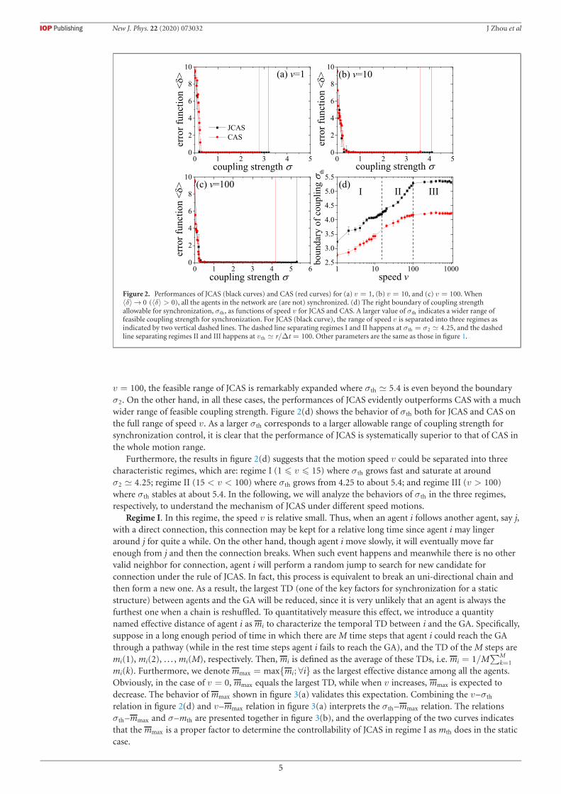
Figure 2. Performances of JCAS (black curves) and CAS (red curves) for (a) v = 1, (b) v = 10, and (c) v = 100. When〈δ〉→ 0 (〈δ〉 > 0), all the agents in the network are (are not) synchronized. (d) The right boundary of coupling strengthallowable for synchronization, σth, as functions of speed v for JCAS and CAS. A larger value of σth indicates a wider range offeasible coupling strength for synchronization. For JCAS (black curve), the range of speed v is separated into three regimes asindicated by two vertical dashed lines. The dashed line separating regimes I and II happens at σth = σ2 � 4.25, and the dashedline separating regimes II and III happens at vth � r/Δt = 100. Other parameters are the same as those in figure 1.

v = 100, the feasible range of JCAS is remarkably expanded where σth � 5.4 is even beyond the boundaryσ2. On the other hand, in all these cases, the performances of JCAS evidently outperforms CAS with a muchwider range of feasible coupling strength. Figure 2(d) shows the behavior of σth both for JCAS and CAS onthe full range of speed v. As a larger σth corresponds to a larger allowable range of coupling strength forsynchronization control, it is clear that the performance of JCAS is systematically superior to that of CAS inthe whole motion range.

Furthermore, the results in figure 2(d) suggests that the motion speed v could be separated into threecharacteristic regimes, which are: regime I (1 � v � 15) where σth grows fast and saturate at aroundσ2 � 4.25; regime II (15 < v < 100) where σth grows from 4.25 to about 5.4; and regime III (v > 100)where σth stables at about 5.4. In the following, we will analyze the behaviors of σth in the three regimes,respectively, to understand the mechanism of JCAS under different speed motions.

Regime I. In this regime, the speed v is relative small. Thus, when an agent i follows another agent, say j,with a direct connection, this connection may be kept for a relative long time since agent i may lingeraround j for quite a while. On the other hand, though agent i move slowly, it will eventually move farenough from j and then the connection breaks. When such event happens and meanwhile there is no othervalid neighbor for connection, agent i will perform a random jump to search for new candidate forconnection under the rule of JCAS. In fact, this process is equivalent to break an uni-directional chain andthen form a new one. As a result, the largest TD (one of the key factors for synchronization for a staticstructure) between agents and the GA will be reduced, since it is very unlikely that an agent is always thefurthest one when a chain is reshuffled. To quantitatively measure this effect, we introduce a quantitynamed effective distance of agent i as mi to characterize the temporal TD between i and the GA. Specifically,suppose in a long enough period of time in which there are M time steps that agent i could reach the GAthrough a pathway (while in the rest time steps agent i fails to reach the GA), and the TD of the M steps aremi(1), mi(2), . . . , mi(M), respectively. Then, mi is defined as the average of these TDs, i.e. mi = 1/M

∑Mk=1

mi(k). Furthermore, we denote mmax = max{mi; ∀i} as the largest effective distance among all the agents.Obviously, in the case of v = 0, mmax equals the largest TD, while when v increases, mmax is expected todecrease. The behavior of mmax shown in figure 3(a) validates this expectation. Combining the v–σth

relation in figure 2(d) and v–mmax relation in figure 3(a) interprets the σth –mmax relation. The relationsσth –mmax and σ–mth are presented together in figure 3(b), and the overlapping of the two curves indicatesthat the mmax is a proper factor to determine the controllability of JCAS in regime I as mth does in the staticcase.

5

New J. Phys. 22 (2020) 073032 J Zhou et al

Figure 3. (a) The behavior of the largest effective distance mmax as a function of speed v for r = 0.1. (b) Comparison betweenthe σ–mth relation of uni-directional chain and the σth –mmax relation derived from the v–mmax and the v–σth relations for thecase of v �= 0.

Figure 4. Behaviors of (a) f, indicating the possibility that an agent fail to find suitable neighbors for connection in a time step,saturates around fth when v > 100, and (b) average survival time of temporal connections th, as a function of v.

We remark that in a certain time step an agent may have a possibility that it fails to find a suitableneighbor to follow. This possibility is equivalent to the fraction of such agents in a time step averaged over along period of time. For convenience, we denote such agent as freely evolving agent and the correspondingpossibility of such event to happen as f. It can be understood that in regime I, so that the motion is slow, fcould be very small [see figure 4(a)] which means an agent i may have valid TDs in most time steps, thusthe introduced mi could be a relevant parameter to reflect the topological relation between it and GA.However, when the speed v further grows into regimes II and III, the possibility f shall also increase, and aconnection is more likely to be broken which may lead the indicator mmax to be deviated from and invalidto describe the actual situation.

Regime III. Now, we turn to the case of regime III, where the speed v > 100 is fast. With the settingr = 0.1, Δt = 10−3 and defining vth = r/Δt = 100, in this regime, an agent will almost certainly separatefrom the followed agent in one time step because of v > vth. Thus, in this regime almost all the connectionsare broken and new connections are formed consistently. This occasion actually makes the network act as afast-varying network. For a fast-varying network, it has been proved that the condition to maintain a stablesynchronization is equivalent to that of a static network which structure is the aggregation of the varyingstructures of the original temporal networks [48]. Therefore, to evaluate the stability of a synchronization inregime III could be transformed to the problem of evaluation on its corresponding aggregated network.

The structure of the aggregated network can be calculated with the following facts. First, as defined inthe JCAS, when an agent is in the disk of radius r centered at the GA, it will definitely follow the GA.Therefore, in each time step an agent has a possibility of b = πr2/L2 to follow the GA directly. Secondly,since an agent has a possibility f to freely evolve (failed to find a proper neighbor to connect) in a time step,the possibility of it following the rest N − 1 agents (except for itself and GA) equals 1 − f − b. As theseN − 1 agents are equal footing, the possibility for each of them to be followed by the agent then equals(1 − f − b)/(N − 1). These facts draw us to the Laplacian matrix G of the aggregation network as⎛

⎜⎜⎜⎜⎜⎜⎜⎜⎜⎜⎜⎝

0 · · · · · · · · · 0

−b 1 − f −1 − f − b

N − 1· · · −1 − f − b

N − 1... −1 − f − b

N − 11 − f

. . ....

......

. . .. . . −1 − f − b

N − 1

−b −1 − f − b

N − 1· · · −1 − f − b

N − 11 − f

⎞⎟⎟⎟⎟⎟⎟⎟⎟⎟⎟⎟⎠

(N+1)×(N+1)

, (4)

6

New J. Phys. 22 (2020) 073032 J Zhou et al

Figure 5. Comparisons for the v–σth relation between the simulation results (black curves) and different measurements for thethree regimes, respectively.

where G11 = 0 (GA is always indexed as 1), G1i = 0 (I � 2), Gi1 = −b (i � 2), Gii = 1 − f (i � 2),Gi�=j = − 1−f−b

N−1 (i � 2, j � 2). Solving the spectrum of G, one gets λ1 = 0 and λ2 = · · · = λN+1 = 1 − f.For this specific case, where connections are consistently broken and agents apply the jump process almostall the time, we denote the possibility that an agent is freely evolving in a time step as fth. The value of fth

could be well estimated (details are provided in the appendix A), and in the setting of N = 100 and r = 0.1,we have fth ≈ 0.22 which is validated by the results in figure 4(a). Now, since the eigenvalue of thetransversal modes of the aggregated network is 1 − fth and the condition for a stable synchronization isΦ(σλ) < 0, the boundary of the coupling strength σth should satisfy σth(1 − f ) = σ2. Inputting σ2 � 4.25and fth ≈ 0.22, we get σth ≈ 5.45. This analytical estimation exhibits good accordance with the simulationresults as shown in figure 5, verifying the fast-varying feature of the network in this regime.

Regime II. Now, we come to the case of regime II. As shown in figure 2(d), in this regime, σth growsgradually with the increasing of v. To better understand this behavior, we take detail observations on thestructural property of temporal networks. First, we measure the average survival time of temporal directedconnections between agents, which is denoted as th. The behavior of th as a function of v is presented infigure 4(b). We can see that it decreases rapidly as the increasing of v in regime I (th →∞ when v = 0). Inthe regimes of II and III, i.e. when v > 15, we observe th < 1.25, which manifests that a connection is notlikely to persist in two consecutive time steps in these regimes. This observation strongly suggests that inregime II the temporal network is also fast-varying.

However, the v–f relation shown in figure 4(a) tells that in the regime II the fraction f is smaller thanthat in the region III. This is due to the fact that an agent with a smaller v may follow its neighbor withmore consecutive time steps as it may take a longer time to move far enough to break the connection. Onthe other hand, if an agent is not following anyone else, the possibility of it finding a proper agent forconnection through the jump process is independent of the motion speed. Combining these two effectsresults in a lower possibility f with a smaller v. Thus, the above observations clearly illustrate that networksin the regime II should still be fast-varying but with a smaller possibility f than that in regime III. Hence,the relation σth = σ2/(1 − f ) is still valid in this regime. By imposing the value of f for different v in regimeII collected from figure 4(a), we obtain the estimated value of σth in the regime II as illustrated in figure 5.We can see that this prediction well matches the simulation results.

3.3. The impact of radius rFinally, we examine the effect of JCAS on different contact radius r. We first present the v–mmax relation ofr = 0.04, 0.06, 0.08, and 0.1 for slow motion regime (regime I) in figure 6(a). One can see that all thesecurves converge to about 2.7, but the curve for a smaller r converges faster. In fact, for a smaller r, aconnection is easier to break since a follower is easier to leave the r-disk of the followed agent. Actually, therate to leave the disk is proportional to v/r, and therefore inversely proportional to the characteristic timethat a connection could preserve. This argument is validated by the rescaled plot in the inset of figure 6(a)where the rescaled behaviors overlap. Then, for fast motion regime (regimes II and III), we show the v–frelation for the same set of r values in figure 6(b). We observe that the behavior of these curves share similartendency. Moreover, as to the v–f relation, besides the rescaling v → v/r, the possibility f is also influencedby r which is encoded in the relation between r and fth (see appendix A). By imposing the rescaling ofv → v/r and f → fth, the rescaled behaviors of v–f relation are shown in the inset of figure 6(b). We can seethat these curves largely conform, revealing the impact of r on f to the performance in these regimes.Further, we present the behaviors of σth as functions of v for the same set of r values in figure 6(c). As

7

New J. Phys. 22 (2020) 073032 J Zhou et al

Figure 6. Behaviors of (a) v–mmax, (b) v–f, and (c) v–σth relations for the case of r = 0.10 (black), r = 0.08 (red), r = 0.06(blue), and r = 0.04 (magenta), respectively. The inset of panel (a) is a rescaled plot of (a) with v → v/r. The inset of panel (b) isa rescaled plot of (b) with v → v/r and f → f/fth. (d) A rescaled plot of (c) with v → v/r and σth → σth (slow motion) orσth → σth(1 − f ) (fast motion). The dashed line separates the two speed motions where σth reaches σ2 � 4.25.

suggested by the scaling properties in figures 6(a) and (b), the v–σth relation should also satisfy similarscaling features. To show this, for each radius r, we separate the speed into slow motion and fast motionwith the condition of σth = σ2 separating the regimes I and II and the condition of vth = r/Δt separatingthe regimes II and III. Then, we rescale the slow motion with v → v/r and fast motion with v → v/r andσth → σth(1 − f ). Resulting behaviors are presented in figure 6(d). Clearly, the overlapping of these rescaledbehaviors under different radius r proves the above conditions classifying the regimes and the effectivenessof related measures.

4. Conclusion

In summary, we have developed the connection adaption strategy (CAS) by introducing a jump process forthe purpose of synchronization control of networks with mobile chaotic agents. The jump process is exertedwhen an agent cannot find a proper neighbor to apply the CAS. Our results have shown that the effect ofjump-based CAS (JCAS) completely outperforms the original CAS. In addition, we have found threedifferent dynamical regimes in JCAS. In the regime where agents move slowly, the network in each time stepcould be characterized by a group of uni-directional chains pointing to the guide agent (GA) which carriesthe target synchronization solution. A measure, referred as the largest topological distance, is introduced todescribe the temporal distance between agents and the GA, which is shown to be a good estimator topredict the controllability of the system in this regime. In the other limit, where agents move very fast, therelations between each pair of agents may change in almost every time step, and the structures between twoconsecutive time steps are largely independent. By analytically calculating the fraction of freely evolvingagents, which temporally fail to find proper neighbors for connection, the range of coupling strengthpermitting successful control is well predicted. For the medium regime of motion speed, we have found thatthe network could also be regarded as fast-varying networks. However, in this regime the fraction of freelyevolving agents varies with the motion speed. We have shown that this fraction grows gradually with theincreasing of the speed, and the range of feasible coupling strength expands from low speed regime to highspeed regime.

For the topic of controlling dynamical systems where individual units could move freely in a space, CASmay have advantage for easier implementation than traditional coupling adaptive strategies. Thejump-based method proposed in this paper could effectively enhance the effectiveness of the CAS. Theprimary role of our work is to emphasize the potential of the CAS scheme. In the current setting, the jumpprocess can be regarded as a high speed movement. However, this process may be generalized by dealingwith the speed of freely evolving agents in a delicate manner applied to more realistic scenarios. As newnetwork perspectives of dynamical systems with varying structures are continuously emerging in theoretical

8

New J. Phys. 22 (2020) 073032 J Zhou et al

Figure A1. Diagram for the evaluation of possibility fth. The GA is located at the center of the plane O. Agent i is located at Oi

which is at a distance R to the O. The two circles (the big one centered at O with radius R and the small one centered at Oi withradius r) intersects at A and B, and overlap in the shaded area. β1 and β2 represent the radians of angle ∠AOOi and ∠AOiO,respectively.

and empirical context [49, 50], further exploitation of the CAS applying to these systems is of futureresearch interest.

Acknowledgments

This work was supported in part by the National Natural Science Foundation of China under Grant11835003, in part by the Ministry of Education, Singapore, under Contract MOE2016-T2-1-119, and inpart by NSF Grant PHY-1505000 and by DTRA Grant HDTRA1-14-1-0017.

Appendix A. Evaluation of fth

In this appendix, we derive the possibility fth that in a time step an agent has no suitable neighbor forconnection when agents continuously jump.

Suppose an agent i located at Oi is at a distance R to the GA located at the center of the plane O (seefigure A1). As defined in the JCAS, if agent i has no suitable neighbor for connection, it means that in thesub-area, which is the overlap between the r-disk centered at Oi and R-disk centered at O (shaded region infigure A1), there is no agent inside it (otherwise a feasible connection is available to agent i). To calculatethe possibility that an agent has no neighbor for connection, we first calculate the area of this shadedregion, denoted as S.

It can be seen that the size of the area S satisfies S = SAOB + S

AOiB− 2SΔAOOi , where S

AOB and SAOiB

are

the areas of sectors AOB and AOiB, respectively, and SΔAOOi is the area of the triangle ΔAOOi. We assumethe radian of the angles ∠AOOi and ∠AOiO are β1 and β2, respectively, then we have S

AOB = 2β1/2π · πR2

and SAOiB

= 2β2/2π · πr2. The SΔAOOi could be calculated with Heron’s formula which gives

SΔAOOi = 1/4√

(2R + r)(2R − r)(R + r − R)(R + r − R)

= r/4√

4R2 − r2. (A.1)

Further with the cosine law cosβ1 = 1 − R2/2r2 and cosβ2 = R/2r, one gets the expression of S as follows

S =

[R2 arccos

(1 − r2

2R2

)+ r2 arccos

( r

2R

)]− r

2

√4R2 − r2. (A.2)

As S/L2 denotes the possibility that a specific agent is in this shaded region, the possibility that none of theN − 1 agents is in this area equals (1 − S)N−1. Further considering the distance between agent i and the GA,we arrive the possibility fth as follows

fth =

∫ rU

rL

(1 − S

L2

)N−1

· 2πR

L2dR. (A.3)

9

New J. Phys. 22 (2020) 073032 J Zhou et al

The lower limit of the integration rL = r since if GA is in the r-disk of agent i, the agent i will directlyconnects the GA, and hence a connection is formed. To evaluate the upper limit rU, we approximate thesquare plane Γ as a circle area with the same area L2, then rU is estimated as the radius of the circle areawhich gives πr2

U = L2, i.e. rU = L/√π. This approximation has a high accuracy when L � r. Applying the

parameter values N = 100, r = 0.1, and L = 1 into equation (7), we obtain fth ≈ 0.22.

ORCID iDs

Jie Zhou https://orcid.org/0000-0001-7006-2889Yinzuo Zhou https://orcid.org/0000-0002-0997-3496

References

[1] Boccaletti S, Kurths J, Osipov G, Valladares D L and Zhou C 2002 The synchronization of chaotic systems Phys. Rep. 366 1[2] Pikovsky A, Rosenblum M and Kurths J 2003 Synchronization: A Universal Concept in Nonlinear Sciences (Cambridge: Cambridge

University Press)[3] Arenas A, Díaz-Guilera A, Kurths J, Moreno Y and Zhou C 2008 Synchronization in complex networks Phys. Rep. 469 93[4] Dorogovtsev S N, Goltsev A V and Mendes J F F 2008 Critical phenomena in complex networks Rev. Mod. Phys. 80 1275[5] Motter A E, Myers S A, Anghel M and Nishikawa T 2013 Spontaneous synchrony in power-grid networks Nat. Phys. 9 191[6] Bullo F, Cortés J and Martínez S 2009 Distributed Control of Robotic Networks (Princeton, NJ: Princeton University Press)[7] Buscarino A, Fortuna L and Frasca M 2006 Dynamical network interactions in distributed control of robots Chaos 16 015116[8] Bartsch R P, Schumann A Y, Kantelhardt J W, Penzel T and Ivanov P C 2012 Phase transitions in physiologic coupling Proc. Natl

Acad. Sci. USA 109 10181[9] Bartsch R P, Liu K K L, Bashan A and Ivanov P C 2015 Network physiology: how organ systems dynamically interact PLoS One 10

e0142143[10] Ivanov P C, Liu K K L and Bartsch R P 2016 Focus on the emerging new fields of network physiology and network medicine New

J. Phys. 18 100201[11] Huang D 2004 Stabilizing near-nonhyperbolic chaotic systems with applications Phys. Rev. Lett. 93 214101[12] Flunkert V, Yanchuk S, Dahms T and Schöll E 2010 Synchronizing distant nodes: a universal classification of networks Phys. Rev.

Lett. 105 254101[13] Schröder M, Mannattil M, Dutta D, Chakraborty S and Timme M 2015 Transient uncoupling induces synchronization Phys. Rev.

Lett. 115 054101[14] Nishikawa T and Motter A E 2010 Network synchronization landscape reveals compensatory structures, quantization, and the

positive effect of negative interactions Proc. Natl Acad. Sci. 107 10342[15] Albert R and Barabási A 2002 Statistical mechanics of complex networks Rev. Mod. Phys. 74 47–97[16] Pastor-Satorras R, Castellano C, Van M P and Vespignani A 2015 Epidemic processes in complex networks Rev. Mod. Phys. 87 925[17] Petter H and Jari S 2012 Temporal networks Phys. Rep. 519 97–125[18] Perra N, Gonçalves B, Pastor-Satorras R and Vespignani A 2012 Activity driven modeling of time varying networks Sci. Rep. 2 469[19] Valdano E, Fiorentin M R, Poletto C and Colizza V 2018 Epidemic threshold in continuous-time evolving networks Phys. Rev.

Lett. 120 068302[20] Koher A, Lentz H, Gleeson J P and Hövel P 2019 Contact-based model for epidemic spreading on temporal networks Phys. Rev. X

9 031017[21] Zhou J, Zou Y, Guan S, Liu Z and Boccaletti S 2016 Synchronization in slowly switching networks of coupled oscillators Sci. Rep.

6 35979[22] Igor V B, Vladimir N B and Martin H 2004 Blinking model and synchronization in small-world networks with a time-varying

coupling Physica D 195 188–206[23] Belykh I, Belykh V and Hasler M 2005 Synchronization in complex networks with blinking interactions Int. Conf. Physics and

Control IEEE pp 86–91[24] Skufca J D and Bollt E M 2004 Communication and synchronization in disconnected networks with dynamic topology: moving

neighborhood networks Math. BioSci. Eng. 1 347[25] Porfiri M, Stilwell D, Erik M B and Skufca J 2006 Random talk: random walk and synchronizability in a moving neighborhood

network Physica D 224 102[26] Porfiri M, Stilwell D, Bollt E M and Skufca J 2007 Stochastic synchronization over a moving neighborhood network Proc. Am.

Control Conf. p 1413[27] Peruani F, Nicola E M and Morelli L G 2010 Mobility induces global synchronization of oscillators in periodic extended systems

New J. Phys. 12 092029[28] Frasca M, Buscarino A, Rizzo A, Fortuna L and Boccaletti S 2008 Synchronization of moving chaotic agents Phys. Rev. Lett. 100

044102[29] Fujiwara N, Kurths J and Díaz-Guilera A 2011 Synchronization in networks of mobile oscillators Phys. Rev. E 83 025101[30] Frasca M, Buscarino A, Rizzo A and Fortuna L 2012 Spatial pinning control Phys. Rev. Lett. 108 204102[31] Dariani R, Buscarino A, Fortuna L and Frasca M 2011 Pinning control in a system of mobile chaotic oscillators AIP Conf. Proc.

1389 1023[32] Klinglmayr J, Kirst C, Bettstetter C and Timme M 2012 Guaranteeing global synchronization in networks with stochastic

interactions New J. Phys. 14 073103[33] Col L D, Tarbouriech S and Zaccarian L 2016 Global H∞ consensus of linear multi-agent systems with input saturation Proc. Am.

Control Conf. p 6272[34] Su H, Chen G, Wang X and Lin Z 2011 Adaptive second-order consensus of networked mobile agents with nonlinear dynamics

Automatica 47 368

10

New J. Phys. 22 (2020) 073032 J Zhou et al

[35] Hu W, Liu L and Feng G 2016 Consensus of linear multi-agent systems by distributed event-triggered strategy IEEE Trans.Cybern. 46 148

[36] Qing H and Haddad W M 2008 Distributed nonlinear control algorithms for network consensus Automatica 44 2375–81[37] Wang X, Su H and Chen G 2017 Fully distributed event-triggered semiglobal consensus of multi-agent systems with input

saturation IEEE Trans. Ind. Electron. 64 5055[38] Zhou J, Zou Y, Guan S, Liu Z, Xiao G and Boccaletti S 2017 Connection adaption for control of networked mobile chaotic agents

Sci. Rep. 7 16069[39] Bartsch R P, Liu K K L, Ma Q D Y and Ivanov P C 2010 Three independent forms of cardio-respiratory coupling: transitions

across sleep stages Comput. Cardiol. 41 781 (PMID: 25664348)[40] Bartsch R P and Ivanov P C 2014 Coexisting forms of coupling and phase-transitions in physiological networks Commun.

Comput. Info. Sci. 438 270[41] Zhu X, Zhou J, Zou Y, Tang M and Xiao G 2019 Enhanced connection adaption strategy with partition approach IEEE Access 7

34162[42] Brock D, Hufnagel L and Geisel T 2006 The scaling laws of human travel Nature 439 462[43] Benhamou S 2007 How many animals really do the Lévy walk? Ecology 88 1962[44] Keeter M, Moore D, Muller R, Nieters E, Flenner J, Martonosi S, Bertozzi A, Percus A and Levy R 2012 Cooperative search with

autonomous vehicles in a 3D aquatic testbed Proc. Am. Control Conf. p 3154[45] Nishikawa T, Motter A E, Lai Y and Hoppensteadt F C 2003 Heterogeneity in oscillator networks: are smaller worlds easier to

synchronize? Phys. Rev. Lett. 91 014101[46] Pecora L M and Carroll T L 1998 Master stability functions for synchronized coupled systems Phys. Rev. Lett. 80 2109[47] Xu L, Chen Z, Hu K, Stanley H E and Ivanov P C 2011 Spurious detection of phase synchronization in coupled nonlinear

oscillators Phys. Rev. E 73 065201[48] Stilwell D, Bollt E M and Roberson G 2006 Synchronization of time-varying networks under fast switching Proc. Am. Control

Conf. 5 140[49] Bashan A, Bartsch R P, Kantelhardt J W, Havlin S and Ivanov P C 2012 Network physiology reveals relations between network

topology and physiological function Nat. Commun. 3 702[50] Ivanov P C and Bartsch R P 2014 Network Physiology: Mapping Interactions Between Networks of Physiologic Networks (Networks

of Networks: The Last Frontier of Complexity) (Berlin: Springer ) ch 10

11