control systems - uniroma1.itlanari/controlsystems/cs... · lanari: cs - control basics ii 7 r (t)...
TRANSCRIPT

Control basics IIL. Lanari
Control Systems
Sunday, November 30, 2014

Lanari: CS - Control basics II 2
Outline
• a general feedback control scheme
• typical specifications
• the 3 sensitivity functions
• constraints in the specification definitions
• steady-state requirements w.r.t. references
• system type
• steady-state requirements w.r.t. disturbances
• effects of the introduction of integrators
• transient characterization in the frequency domain
• closed-loop to open-loop transient specifications
Sunday, November 30, 2014

Lanari: CS - Control basics II 3
general feedback control scheme
controlledsystem
controlledvariable/output
disturbances
controller
transducer
reference
+ -
all this is “built” on top of the system to be controlled
this choice will influence therefore the type of measurement noise present
we concentrate on the choice of the controller
measurement noise
Sunday, November 30, 2014

Lanari: CS - Control basics II 4
general feedback control scheme
controlledsystem
controller+ -
• r (t) reference signal
• e (t) error
• m (t) control input
• d (t) disturbance
• y (t) controlled output
• n (t) measurement noise
r (t) e (t) m (t)
d (t)
y (t)
n (t)
controllerC (s)
(Ac, Bc, Cc, Dc)
�
equivalent(since we design the controller)
Sunday, November 30, 2014

Lanari: CS - Control basics II 5
+ model for the controlled system (plant)
+ -
r (t) e (t) m (t) y (t)
n (t)
+
+
P (s)C (s)
u (t)
d1(t) d2(t)
distinguish if the disturbance acts at the input of the plant d1(t) or at the output d2(t)
signals d1(t), d2(t) and n (t) may be the output of some other system too
transducer n (t)
d3(t)
H (s)
d3(t)
+
+
+++
+
Sunday, November 30, 2014

Lanari: CS - Control basics II 6
+ -
r (t)
e (t) m (t)
y (t)
n (t)
+
+
P (s)C (s)
u (t)
d1(t) d2(t)
++++
r (t)
d1(t)
d2(t)
n (t)
e (t)
m (t)
y (t)
• several inputs act simultaneously on the control system
• we may be interested in several variables
control system
Sunday, November 30, 2014

Lanari: CS - Control basics II 7
r (t)
d1(t)
d2(t)
n (t)
e (t)
m (t)
y (t)control system
we may need to give specifications on different pairs (Input, Output)
the effect of each input on any output is determined using the superposition principle that is
by considering each input at a time (for example if we want to determine the effect of the
input r (t) on m (t) we set d1(t) = d2(t) = n (t) = 0 and compute the single input - single
output transfer function from r (t) to m (t))
Sunday, November 30, 2014

Lanari: CS - Control basics II 8
define the loop function L(s) = C(s)P (s) and
S(s) =1
1 + L(s)
T (s) =L(s)
1 + L(s)
Su(s) =C(s)
1 + L(s)
sensitivity function
complementary sensitivity function
control sensitivity function
check that, using the superposition principle,
since S (s) + T (s) = 1
y(s) = T (s)r(s) + P (s)S(s)d1(s) + S(s)d2(s)− T (s)n(s)
e(s) = S(s)r(s)− P (s)S(s)d1(s)− S(s)d2(s)− S(s)n(s)
m(s) = Su(s)r(s)− T (s)d1(s)− Su(s)d2(s)− Su(s)n(s)
Sunday, November 30, 2014

Lanari: CS - Control basics II 9
Model uncertainties (plant)
• Parametric uncertainties:
the real (perturbed) parameters of the controlled system are different from the ones
(nominal) used to design the controller
- slowly time-varying parameters
- wear & tear (damage caused by use)
- difficulty to determine true values
- change of operating conditions (linearization), ...
• Un-modeled dynamics:
typically high-frequency
- dynamics deliberately neglected for design simplification,
- difficulty in modeling
Sunday, November 30, 2014

Lanari: CS - Control basics II 10
Parametric uncertainties(MSD example)
10 1 100 10130
20
10
0
10
20
frequency
Mag
(dB)
10 1 100 101
150
100
50
0
frequency
Phas
e
5 4 3 2 1 0 1 2 3 4 58
7
6
5
4
3
2
1
0
1
Real
Imag
Uncertainties for = 1, 1.5, 2, 3 rad/s
1.5 1 0.5 0 0.51
0.8
0.6
0.4
0.2
0
0.2
0.4
0.6
0.8
1
Real
Imag
Zoom of uncertainties for = 1, 1.5, 2, 3 rad/s
m in [0.9, 1.1]
µ in [0.05, 2]
k in [2, 3]
zoom
!1 = 1 rad/s!2 = 1.5 rad/s!3 = 2 rad/s!4 = 3 rad/s
Nyquistplot
P (s) =1
ms2 + µs+ k
Sunday, November 30, 2014

Lanari: CS - Control basics II 11
This example illustrates the dangers of designing a controller (static K = 1 in this case) based on dominant dynamics
-1-40 Re
Im
full dynamics
dominantdynamics
same gain as F2(s) but only dominant dynamics (approximation)
Un-modeled dynamics
F2(s) =100
(s+ 1)(0.025s+ 1)2
F1(s) =100
s+ 1
Sunday, November 30, 2014

Lanari: CS - Control basics II 12
open-loop similar
20 0 20 40 60 80 100 12060
40
20
0
20
40
60
Nyquist Diagram
Real Axis
Imag
inar
y Ax
is
4 3 2 1 0 1 25
4
3
2
1
0
1
2
3
4
5
Nyquist Diagram
Real Axis
Imag
inar
y Ax
is
zoom
10 2 100 10240
20
0
20
40
Freq (rad/s)
Mag
(dB)
F1(s)
10 2 100 10240
20
0
20
40
Freq (rad/s)
Mag
(dB)
F2(s)
100
250
200
150
100
50
0
Freq (rad/s)
Phas
e
F1(s)
100
250
200
150
100
50
0
Freq (rad/s)
Phas
e
F2(s)
unstable dynamics (Nyquist criterion)
differ in high frequency content
F1(s) =100
s+ 1F2(s) =100
(s+ 1)(0.025s+ 1)2
W1(s) =100
s+ 101
W2(s) =160000
(s+ 83.9254)(s2 − 2.9254s+ 1925.5)
simplified model with onlythe dominant dynamics
but closed-loop different
stable
F1 (j!)F2 (j!)
Sunday, November 30, 2014

Lanari: CS - Control basics II 13
Specifications
Stability of the control system (closed-loop system)
• nominal stability (can be checked with Routh, Nyquist, root locus ...)
• robust stability guarantees that, even in the presence of parameter uncertainty
and/or un-modeled dynamics, stability of the closed-loop system is guaranteed. We
have seen two useful indicators (gain and phase margins) others are possible (based on
the Nyquist stability criterion or on a surprising result known as the Kharitonov
theorem).
Performance
• nominal performance
- static (or at steady-state) on the desired behavior between the different input/
output pairs of interest
- dynamic: on the dynamic behavior during transient
• robust performance: we ask that the performance obtained in nominal conditions
is also guaranteed, to some extent, under perturbations (parameter variations, un-
modeled dynamics).
Sunday, November 30, 2014
Lanari: CS - Control basics II 14
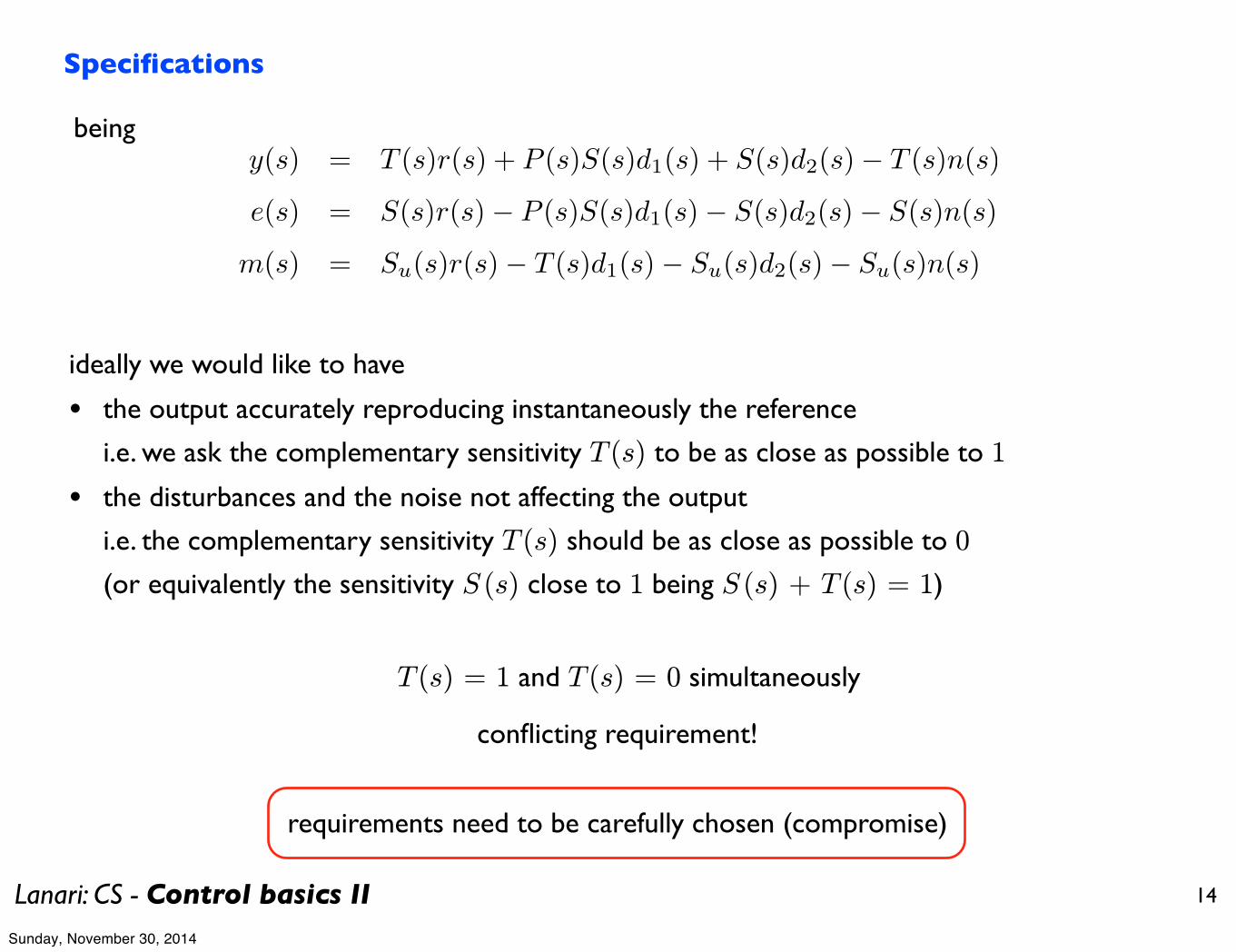
Specifications
being
ideally we would like to have
• the output accurately reproducing instantaneously the reference
i.e. we ask the complementary sensitivity T (s) to be as close as possible to 1
• the disturbances and the noise not affecting the output
i.e. the complementary sensitivity T (s) should be as close as possible to 0
(or equivalently the sensitivity S (s) close to 1 being S (s) + T (s) = 1)
T (s) = 1 and T (s) = 0 simultaneously
conflicting requirement!
requirements need to be carefully chosen (compromise)
y(s) = T (s)r(s) + P (s)S(s)d1(s) + S(s)d2(s)− T (s)n(s)
e(s) = S(s)r(s)− P (s)S(s)d1(s)− S(s)d2(s)− S(s)n(s)
m(s) = Su(s)r(s)− T (s)d1(s)− Su(s)d2(s)− Su(s)n(s)
Sunday, November 30, 2014

Lanari: CS - Control basics II 15
Specifications
example
• static (at steady-state) reference/output behavior w.r.t. standard signals (sinusoidal
or polynomial)
• static disturbance/output behavior for some standard signal (sinusoidal or constant)
• dynamic (transient) reference/output behavior
- by setting limits to the step response parameters like overshoot or rise time
- by setting some equivalent bounds on the frequency response (bandwidth,
resonance peak defined soon)
+ closed-loop stabilitymost important requirementalways present even if not explicitly stated
note how we relaxed some requirements on the performance w.r.t. reference and disturbance by asking the fulfillment only at steady-state that is
limt→∞
(r(t)− y(t)) = 0 y(t) = r(t), ∀tinstead of
Sunday, November 30, 2014

Lanari: CS - Control basics II 16
Steady-state specifications - reference
Hyp: closed-loop system will be asymptotically stable
Let the canonical signal of order k be
tk
k!δ−1(t)
order 0 (step function)
order 1 (ramp function)
order 2 (quadratic function)
δ−1(t)
tδ−1(t)
t2
2δ−1(t)
t
t
t
Sunday, November 30, 2014

Lanari: CS - Control basics II 17
Def a system is of type k if its steady-state response to an input of order k differs
from the input by a non-zero constant or, equivalently, if the error at state-state (output
minus input) is constant and different from zero.
t t
type 0 type 1
y (t)
y (t)e0
e1
apply this definition to a feedback control system where the input is the reference
signal and the output is the controlled output and we look for conditions which
guarantee that a feedback system is of type k
Sunday, November 30, 2014
Lanari: CS - Control basics II 18
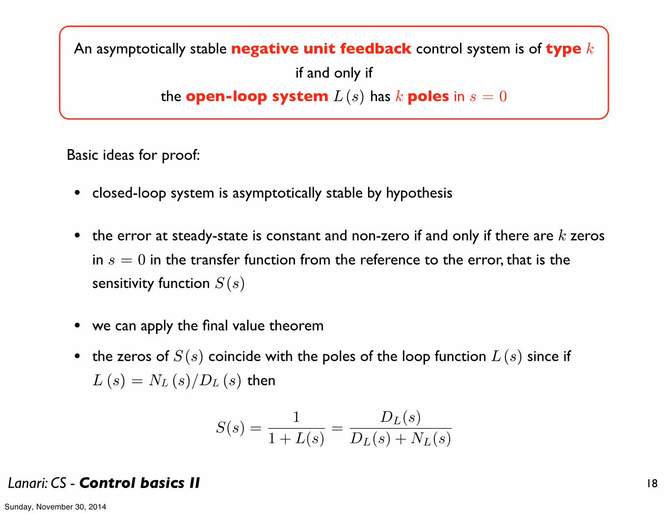
An asymptotically stable negative unit feedback control system is of type k
if and only if
the open-loop system L (s) has k poles in s = 0
Basic ideas for proof:
• closed-loop system is asymptotically stable by hypothesis
• the error at steady-state is constant and non-zero if and only if there are k zeros
in s = 0 in the transfer function from the reference to the error, that is the
sensitivity function S (s)
• we can apply the final value theorem
• the zeros of S (s) coincide with the poles of the loop function L (s) since if
L (s) = NL (s)/DL (s) then
S(s) =1
1 + L(s)=
DL(s)
DL(s) +NL(s)
Sunday, November 30, 2014

Lanari: CS - Control basics II 19
• order k = 0 reference
Define with KP and KC the generalized gain respectively of the plant and the controller,
therefore the generalized gain of the loop function L (s) is KL = KP KC
• order referencek ≥ 1
e0 = S(0) =
11+KL
if Type 0
0 if Type k ≥ 1
ek = lims→0
�sS(s)
1
sk+1
�=
∞ if Type < k
1KL
if Type = k
0 if Type > k
since the presence of 1 or more roots in s = 0 in the denominator DL (s) of the
loop function makes the numerator of S (s) become zero
if the denominator DL (s) has roots in s = 0 with multiplicity h, we factor DL (s) as
s hD’L (s) such that KL = NL (0)/D’L (0). We obtain the different situations
depending on the multiplicity h, that is h < k, h = k and h > k
Sunday, November 30, 2014

Lanari: CS - Control basics II
δ−1(t)1
1 +KL
tδ−1(t) +∞ 1
KL
t2
2δ−1(t) +∞ +∞ 1
KL
t3
3!δ−1(t) +∞ +∞ +∞ 1
KL
error
0 1 2 3
0 0 0 0
1 0 0
2 0
3
20
Summarizing table: error w.r.t. the reference
Input order
System type
Sunday, November 30, 2014

Lanari: CS - Control basics II 21
Therefore
we can define the specifications on the reference to output behavior in terms of system type
and value of maximum allowable error or, equivalently,
• presence of the sufficient number of poles in s = 0 in the open-loop system
• absolute value of the open-loop gain KL sufficiently large in order to guarantee the
maximum allowed error
|ek| ≤ ekmax ⇐⇒
1|1+KL| ≤ ekmax ⇔ |1 +KL| ≥ 1
ekmaxif Type 0
1|KL| ≤ ekmax ⇔ |KL| ≥ 1
ekmaxif Type k ≥ 1
We have translated the closed-loop specifications in equivalent open-loop ones
C (s) P (s)
SOL
control system
SCL
specsr (t)
e (t)y (t)
Sunday, November 30, 2014

Lanari: CS - Control basics II 22
Steady-state specifications - disturbance
The disturbance is just another - undesired - input.
Let us consider the constant disturbance input case and use the same basic principle as
for the reference.
To make an asymptotically stable control system controlled output insensible (astatic), at
steady-state, to a constant input d1 or d2, we just need to ensure the presence of a pole in s
= 0 before the entering point of the disturbance.
+ -
r (t) e (t) m (t) y (t)
n (t)
+
+
P (s)C (s)
u (t)
d1(t) d2(t)
+++
+
Let’s check
Note that nothing is said for the noise n
Sunday, November 30, 2014

Lanari: CS - Control basics II 23
y(s) = T (s)r(s) + P (s)S(s)d1(s) + S(s)d2(s)− T (s)n(s)
constant unit disturbances
d1(s) = d2(s) = n(s) =1
sbeing
we have (setting the reference to zero)
yss = [P (s)S(s)]s=0 + S(0)− T (0)
therefore we need to compute the value of the terms
C(s) =NC(s)
DC(s)P (s) =
NP (s)
DP (s)L(s) =
NL(s)
DL(s)=
NC(s)NP (s)
DC(s)DP (s)define
d1
d2
n
yss
yss
yss
[P (s)S(s)]s=0
S (0)
- T (0)
Sunday, November 30, 2014

Lanari: CS - Control basics II 24
• to have no steady-state contribution to the output yss from a constant disturbance d2 we
need to have S (0) = 0 that is, being
the zeros of the sensitivity function S (s) coincide with the poles of the loop function L (s)
so we will have S (0) = 0 (i.e. s = 0 is a zero of S (s)) if and only if we have at least one
pole at the origin in the open-loop system (and for this disturbance, this is equivalent to
asking at least a pole in s = 0 before the entry point of the disturbance).
S(s) =1
1 + L(s)=
DL(s)
DL(s) +NL(s)=
DC(s)DP (s)
DL(s) +NL(s)=
DC(s)DP (s)
DP (s)DP (s) +NC(s)NP (s)
d2 yss
so either a pole in s = 0 is already present in the plant or we need to introduce it in the
controller (necessary part of the controller to cancel out the effect of the constant
disturbance d2 at steady-state on the output).
Sunday, November 30, 2014

Lanari: CS - Control basics II 25
if no pole in s = 0 is present in loop we have a steady-state effect of a constant unit
disturbance d2 given by
yss = S(0) =1
1 +KL=
1
1 +KCKP
so a high-gain controller will reduce the effect of the given disturbance provided the system
remains asymptotically stable
Sunday, November 30, 2014

Lanari: CS - Control basics II 26
• for the steady-state contribution to the output yss of a constant disturbance d1 note that
P (s)S(s) =NP (s)DC(s)
DP (s)DP (s) +NC(s)NP (s)
therefore in order to get a zero contribution at steady-state we can either
- have a pole in s = 0 in C (s) (ahead of the entry point of the disturbance) or
- have a zero in s = 0 in P (s) but this leads also to a zero steady-state contribution of
a constant reference to the output, i.e. zero gain T (0) = 0 while we would like this
gain to be as close to 1 as possible (avoid when possible)
otherwise we have a finite non-zero contribution given by
KP
1 +KPKC
1
KC
if P (s) has no poles in 0
if P (s) has poles in 0
proof as exercise
d1 yss
Sunday, November 30, 2014

Lanari: CS - Control basics II 27
• for the steady-state contribution to the output yss of a constant noise n note that
T (s) =NP (s)NC(s)
DP (s)DP (s) +NC(s)NP (s)
therefore in order to get a zero contribution at steady-state we can either
- have a zero in s = 0 in P (s) and or C (s) but this leads also to a zero steady-state
contribution of a constant reference to the output, i.e. zero gain T (0) = 0 while we would
like this gain to be as close to 1 as possible (avoid when possible)
otherwise we have a finite non-zero contribution given by
KPKC
1 +KPKCif L (s) has no poles in 0
if L (s) has poles in 01
n yss
High-gain makes things worse w.r.t. noise disturbance
Sunday, November 30, 2014

Lanari: CS - Control basics II 28
-1
Im
Re
Effect of integrators on stabilityThe previous analysis has shown that, provided the control system remains stable, adding
integrators in the forward path has beneficial effects on the steady-state behavior of the closed-
loop system.
However integrators in the open-loop system have a destabilizing effect on the closed-
loop as shown in the following Nyquist plot or equivalently by noting the lag effect on the phase
(-¼/2 for each pole in 0). In the design process we will introduce the minimum number of
integrators necessary.
the shown Nyquist plot are not complete
since it’s only for ! in (0+, + ∞)
type 0
type 1
type 2
type 2
depends upon
the other poles
in L (s)
Sunday, November 30, 2014

Lanari: CS - Control basics II 29
Other steady-state requirements• asymptotic tracking of a sinusoidal function. Let the reference be (for positive t)
r(t) = sin ω̄t r(s) =ω̄
s2 + ω̄2
e(s)
r(s)=
r(s)− y(s)
r(s)= S(s)
ess(t) = |S(jω̄)| sin(ω̄t+ ∠S(jω̄))
with Laplace transform
to asymptotically track this reference the controlled output needs to tend asymptotically
to the reference or, equivalently, the difference (error signal) r (t) - y (t) needs to tend to
zero as t tends to infinity. Recalling that the transfer function from the reference to the
error is
and that, for an asymptotically stable system, the steady-state response to a sinusoidal is
it is clear that, in order to achieve zero asymptotic error we need, at the specific input
frequency, to be able to ensure that
|S(jω̄)| = 0 S(s)���s=jω̄
= 0⇐⇒
Sunday, November 30, 2014

Lanari: CS - Control basics II 30
that is the sensitivity function must have a pure imaginary zero (and its conjugate) at the
frequency of the input signal ω̄
from the previous analysis we also know that the zeros of the sensitivity function coincide
with the poles of the open-loop function (in a unit feedback scheme), therefore the necessary
and sufficient condition becomes
in order to guarantee asymptotic tracking of a sinusoid of frequency in an
asymptotically stable feedback system, the open-loop system needs to have a
pair of conjugate poles in s = ±jω̄
ω̄
Being L(s) = C(s)P (s) and assuming that the plant has no poles in the controller
needs to be of the form
s = ±jω̄
C(s) =NC(s)
(s2 + ω̄2)D�C(s)
Sunday, November 30, 2014

Lanari: CS - Control basics II 31
• asymptotic rejection of a sinusoidal disturbance (similarly)
Assuming that the plant has no poles in the controller needs to be of the forms = ±jω̄
d1(t) = sin ω̄t
d2(t) = sin ω̄t
d1
d2
yss
yss |S(jω̄)| = 0
[P (s)S(s)]s=jω̄ = 0|P (jω̄)S(jω̄)| = 0
S(s)���s=jω̄
= 0
C(s) =NC(s)
(s2 + ω̄2)D�C(s)
Sunday, November 30, 2014
Lanari: CS - Control basics II 32
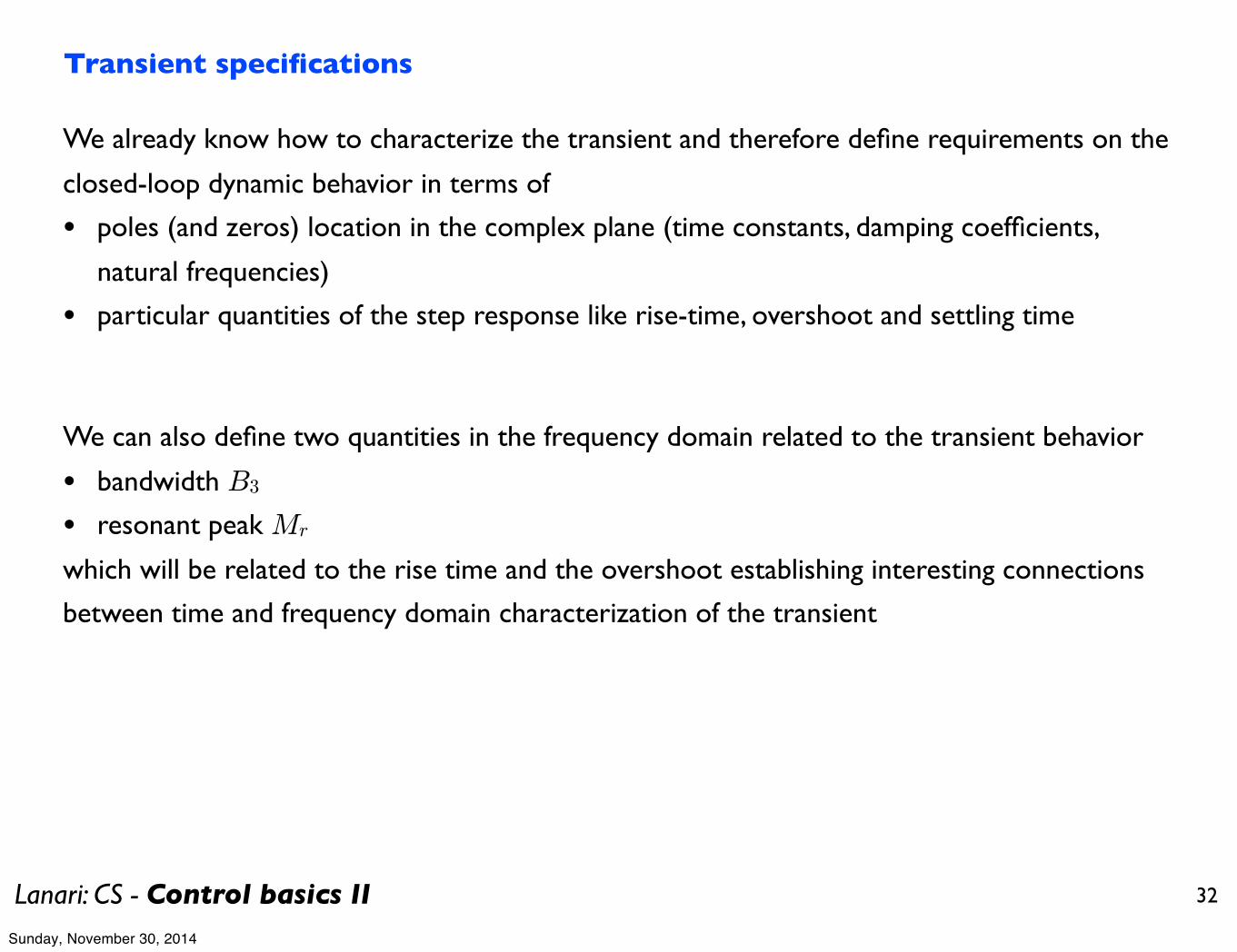
Transient specifications
We already know how to characterize the transient and therefore define requirements on the
closed-loop dynamic behavior in terms of
• poles (and zeros) location in the complex plane (time constants, damping coefficients,
natural frequencies)
• particular quantities of the step response like rise-time, overshoot and settling time
We can also define two quantities in the frequency domain related to the transient behavior
• bandwidth B3
• resonant peak Mr
which will be related to the rise time and the overshoot establishing interesting connections
between time and frequency domain characterization of the transient
Sunday, November 30, 2014

Lanari: CS - Control basics II 33
Bandwidth
for the typical magnitude plots encountered so far, we define the bandwidth
B3 as the first frequency such that for all frequencies greater than the
bandwidth the magnitude is attenuated by a factor greater than
from its value in ! = 0
1/√2
20 log10
�1√2
�≈ −3 dB
|W (jB3)| =|W (j0)|√
2
|W (jB3)|dB = |W (j0)|dB − 3
B3 :
and being
B3 :
Sunday, November 30, 2014

Lanari: CS - Control basics II 34
!40
!30
!20
!10
!30
10
frequency (rad/s)
Magnitude (dB)
1/| ¿ |
simplest example
asymptotically stable system (therefore ¿ > 0)
B3 =1
τ
W (s) =K
1 + τs
normalized w.r.t.
|K|dB magnitude
plot
being
and
|W (jω)|dB − |W (j0)|dB = |W (jω)|dB − |K|dB= |K|dB + |1/(1 + jωτ)|dB − |K|dB= |1/(1 + jωτ)|dB
|1 + jτ/|τ | |dB = 20 log10√2 ≈ 3 dB
the bandwidth coincides with the cutoff frequency
Sunday, November 30, 2014
Lanari: CS - Control basics II 35
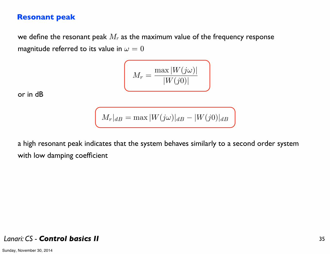
Resonant peak
we define the resonant peak Mr as the maximum value of the frequency response
magnitude referred to its value in ! = 0
Mr =max |W (jω)|
|W (j0)|
Mr|dB = max |W (jω)|dB − |W (j0)|dB
or in dB
a high resonant peak indicates that the system behaves similarly to a second order system
with low damping coefficient
Sunday, November 30, 2014

Lanari: CS - Control basics II 36
on a plot with normalized magnitude (not in dB)
|W (jω)||W (j0)|
ω
1
Mr
1√2
B3
Sunday, November 30, 2014

Lanari: CS - Control basics II 37
Relationships
B3 tr ≈ constant
1 +Mp
Mr≈ constant
typically (with some exceptions)
higher bandwidth (higher frequency components of the input signal are not attenuated and
therefore are allowed to go through) leads to smaller rise time (faster system response)
higher resonant peak (as if we had a second order system with lower damping coefficient)
leads to higher overshoot (the oscillation damps out slower)
very useful relationships in order to understand the connections between time and
frequency domain response characteristics
Sunday, November 30, 2014
Lanari: CS - Control basics II 38
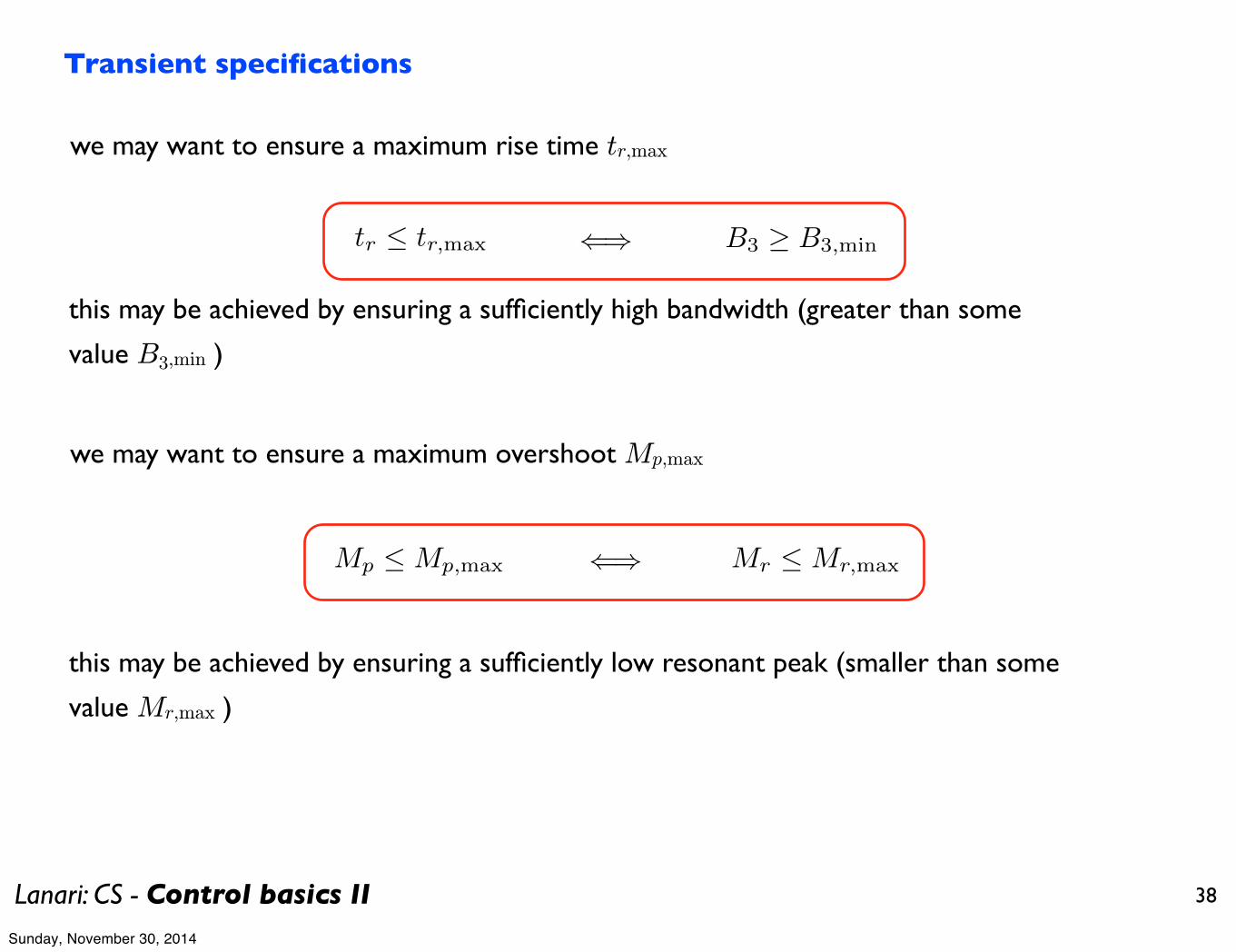
we may want to ensure a maximum rise time tr,max
Transient specifications
tr ≤ tr,max B3 ≥ B3,min
Mp ≤ Mp,max Mr ≤ Mr,max
⇐⇒
this may be achieved by ensuring a sufficiently high bandwidth (greater than some
value B3,min )
we may want to ensure a maximum overshoot Mp,max
this may be achieved by ensuring a sufficiently low resonant peak (smaller than some
value Mr,max )
⇐⇒
Sunday, November 30, 2014
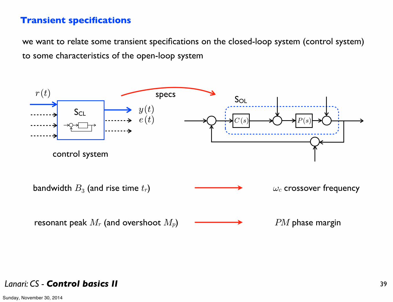
Lanari: CS - Control basics II 39
Transient specifications
C (s) P (s)
SOL
control system
SCL
specsr (t)
e (t)y (t)
we want to relate some transient specifications on the closed-loop system (control system)
to some characteristics of the open-loop system
bandwidth B3 (and rise time tr)
resonant peak Mr (and overshoot Mp)
! c crossover frequency
PM phase margin
Sunday, November 30, 2014

Lanari: CS - Control basics II 40
we show these typical (with some exceptions) relationships through an example
10!1
100
101
102
!40
!20
0
20
frequency (rad/s)
Magnitude (dB)
K = 0.3K = 2K = 6
!1 !0.8 !0.6 !0.4 !0.2 0 0.2
!0.6
!0.4
!0.2
0
0.2
0.4
0.6
Im
Re
K = 0.3
K = 2
K = 6
10!1
100
101
102
!270
!180
!90
0
Phase (deg)
frequency (rad/s)
F (s) =10K
s(s+ 10)(s+ 1)open-loop system
10!1
100
101
102
0
5
10
frequency (rad/s)
Magnitude (NOT in dB)
K = 0.5K = 0.8K = 1.2K = 1.6
comparison for increasing values of K
open-loop phase margin PM decreases
closed-loop resonant peak Mr increases&
PM and Mr relationship
recall that if the Nyquist
plot goes through the
critical point then the
closed-loop system has pure
imaginary poles (zero
damping and thus infinite
resonant peak)
Sunday, November 30, 2014

Lanari: CS - Control basics II 41
10!1
100
101
102
!40
!20
0
20
frequency (rad/s)
Magnitude (dB)
K = 0.3K = 2K = 6
10!1
100
101
102
!5
!3
0
5
10Closed!loop system
frequency (rad/s)
Magnitude (dB)
K = 0.5K = 0.8K = 1.2K = 1.6
same open-loop system comparison for increasing values of K
!c and B3 relationship
as the open-loop crossover frequency !c increases the closed-loop bandwidth B3 increases
!cB3
Sunday, November 30, 2014
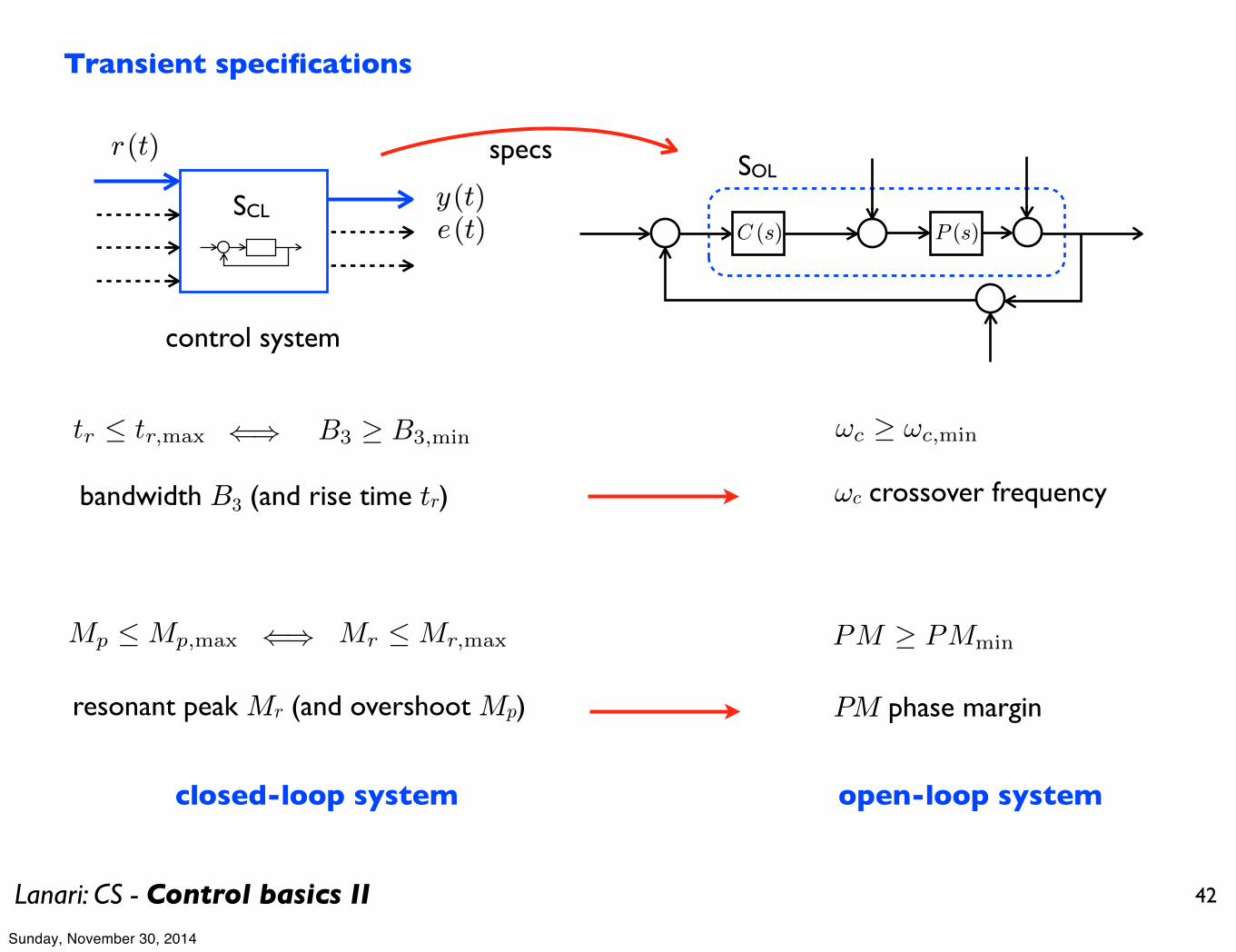
Lanari: CS - Control basics II 42
C (s) P (s)
SOL
control system
SCL
specsr (t)
e (t)y (t)
bandwidth B3 (and rise time tr)
resonant peak Mr (and overshoot Mp)
! c crossover frequency
PM phase margin
Transient specifications
tr ≤ tr,max B3 ≥ B3,min⇐⇒ ωc ≥ ωc,min
PM ≥ PMminMp ≤ Mp,max Mr ≤ Mr,max⇐⇒
closed-loop system open-loop system
Sunday, November 30, 2014