Controllability of the Navier-Stokes equation in a rectanglewith a little help of a distributed phantom force

Jean-Michel Coron∗†, Frédéric Marbach‡, Franck Sueur§, Ping Zhang¶

February 2, 2018

Abstract

We consider the 2D incompressible Navier-Stokes equation in a rectangle with theusual no-slip boundary condition prescribed on the upper and lower boundaries. Weprove that for any positive time, for any finite energy initial data, there exist controlson the left and right boundaries and a distributed force, which can be chosen arbitrarilysmall in any Sobolev norm in space, such that the corresponding solution is at rest atthe given final time.

Our work improves earlier results in [17, 18] where the distributed force is small onlyin a negative Sobolev space. It is a further step towards an answer to Jacques-LouisLions’ question in [23] about the small-time global exact boundary controllability of theNavier-Stokes equation with the no-slip boundary condition, for which no distributedforce is allowed.

Our analysis relies on the well-prepared dissipation method already used in [28]for Burgers and in [9] for Navier-Stokes in the case of the Navier slip-with-frictionboundary condition. In order to handle the larger boundary layers associated withthe no-slip boundary condition, we perform a preliminary regularization into ana-lytic functions with arbitrarily large analytic radius and prove a long-time nonlin-ear Cauchy-Kovalevskaya estimate relying only on horizontal analyticity, in the spiritof [3, 35].

∗Laboratoire Jacques-Louis Lions, Université Pierre et Marie Curie, 4 place Jussieu, 75252 Paris cedex05; France, coron@ann.jussieu.fr

†ETH Zurich Institute for Theoretical Studies Clausiusstrasse 47 8092 Zurich; Switzerland‡Univ Rennes, CNRS, IRMAR - UMR 6625, F-35000 Rennes, France, marbach@ann.jussieu.fr§Institut de Mathématiques de Bordeaux, Université de Bordeaux, 351 cours de la libération, 33405

Talence; France, franck.sueur@math.u-bordeaux.fr¶Academy of Mathematics & Systems Science and Hua Loo-Keng Key Laboratory of Mathematics, The

Chinese Academy of Sciences, Beijing 100190; China, zp@amss.ac.cn

1

arX

iv:1

801.

0186

0v2

[m

ath.

AP]

1 F

eb 2

018

Contents

1 Introduction and statement of the main result 31.1 Historical context . . . . . . . . . . . . . . . . . . . . . . . . . . . . . . . . . 31.2 Statement of the main result . . . . . . . . . . . . . . . . . . . . . . . . . . 31.3 Comments and references . . . . . . . . . . . . . . . . . . . . . . . . . . . . 41.4 Strategy of the proof and plan of the paper . . . . . . . . . . . . . . . . . . 5

2 Regularization enhancement 82.1 Fourier analysis in the tangential direction . . . . . . . . . . . . . . . . . . . 82.2 Regularization enhancement using the phantom and the control . . . . . . . 92.3 Proof of the regularization proposition . . . . . . . . . . . . . . . . . . . . . 10

3 Strategy for global approximate controllability 113.1 Small-time to small-viscosity scaling . . . . . . . . . . . . . . . . . . . . . . 113.2 Return method ansatz . . . . . . . . . . . . . . . . . . . . . . . . . . . . . . 113.3 Estimates and proof of approximate controllability . . . . . . . . . . . . . . 133.4 Comments and insights on the proposed expansion . . . . . . . . . . . . . . 15

4 Well-prepared dissipation method for the boundary layer 164.1 Large time decay of the boundary layer profile . . . . . . . . . . . . . . . . . 164.2 Fast variable scaling and Lebesgue norms . . . . . . . . . . . . . . . . . . . 174.3 Estimates for the technical profile . . . . . . . . . . . . . . . . . . . . . . . . 184.4 Proof of the decay of approximate trajectories . . . . . . . . . . . . . . . . . 18

5 Estimates on the remainder 195.1 Singular amplification to loss of derivative . . . . . . . . . . . . . . . . . . . 205.2 A few tools from Littlewood-Paley theory . . . . . . . . . . . . . . . . . . . 205.3 Long-time weakly nonlinear Cauchy-Kovalevskaya estimate . . . . . . . . . . 245.4 Proof of Proposition 5.10 . . . . . . . . . . . . . . . . . . . . . . . . . . . . . 275.5 Estimate of (r · ∇)u1 + (u1 · ∇)r. Proof of Lemma 5.14 . . . . . . . . . . . . 295.6 Estimate of (r · ∇)r. Proof of Lemma 5.15 . . . . . . . . . . . . . . . . . . . 31

6 Analytic estimates for the approximate trajectories 376.1 Preliminary estimates . . . . . . . . . . . . . . . . . . . . . . . . . . . . . . 376.2 Estimates for the amplification terms . . . . . . . . . . . . . . . . . . . . . . 386.3 Estimates for the source terms . . . . . . . . . . . . . . . . . . . . . . . . . 39

2

1 Introduction and statement of the main result

1.1 Historical context

In the late 1980’s, Jacques-Louis Lions introduced in [23] (see also [24, 25, 26]) the questionof the controllability of fluid flows in the sense of how the Navier-Stokes system can bedriven by a control of the flow on a part of the boundary to a wished plausible state, say avanishing velocity. Jacques-Louis Lions’ problem has been solved in [9] by the first threeauthors in the particular case of the Navier slip-with-friction boundary condition (see also[10] for a gentle introduction to this result). In its original statement with the no-slipDirichlet boundary condition, it is still an important open problem in fluid controllability.

1.2 Statement of the main result

In this paper we consider the case where the flow occupies a rectangle, where controls areapplied to the lateral boundaries and the no-slip condition is prescribed on the upper andlower boundaries. We thus consider a rectangular domain

Ω := (0, L)× (−1, 1),

where L > 0 is the length of the domain. We will use (x, y) as coordinates. Inside thisdomain, a fluid evolves under the Navier-Stokes equation. We will name u = (u1, u2) thetwo components of its velocity. Hence, u satisfies:

∂tu+ (u · ∇)u+∇p−∆u = fg,

div u = 0,(1.1)

in Ω, where p denotes the fluid pressure and fg a force term (to be detailed below). Wethink of this domain as a river or a tube and we assume that we are able to act on thefluid flow at both end boundaries:

Γ0 := 0 × (−1, 1) and ΓL := L × (−1, 1).

On the remaining parts of the boundary,

Γ± := (0, L)× ±1,

we assume that we cannot control the fluid flow and that it satisfies null Dirichlet boundaryconditions:

u = 0 on Γ±. (1.2)

We will consider initial data in the space L2div(Ω) of divergence free vector fields, tangent

to the boundaries Γ±. The main result of this paper is the following.

Theorem 1. Let T > 0 and u∗ in L2div(Ω). For any k ∈ N and for any η > 0, there exists

a force fg ∈ L1((0, T );Hk(Ω)) satisfying

‖fg‖L1((0,T );Hk(Ω)) ≤ η (1.3)

and an associated weak Leray solution u ∈ C0([0, T ];L2div(Ω)) ∩ L2((0, T );H1(Ω)) to (1.1)

and (1.2) satisfying u(0) = u∗ and u(T ) = 0.

3

Since the notion of weak Leray solution is classically defined in the case where the nullDirichlet boundary condition is prescribed on the whole boundary, let us detail that we saythat u ∈ C0([0, T ];L2

div(Ω))∩L2((0, T );H1(Ω)) is a weak Leray solution to (1.1) and (1.2)satisfying u(0, ·) = u∗ and u(T, ·) = 0 when it satisfies the weak formulation

−∫ T

0

∫Ωu · ∂tϕ+

∫ T

0

∫Ω

(u · ∇)u · ϕ+ 2

∫ T

0

∫ΩD(u) : D(ϕ)

=

∫Ωu∗ · ϕ(0, ·) +

∫ T

0

∫Ωu · fg,

(1.4)

for any test function ϕ ∈ C∞([0, T ]×Ω) which is divergence free, tangent to Γ±, vanishes att = T and vanishes on the controlled parts of the boundary Γ0 and ΓL. Thus, (1.4) encodesthe no-slip condition on the upper and lower boundaries only. This under-determinationencodes that one has control over the remaining part of the boundary, that is on thelateral boundaries. The controls on the lateral boundaries are therefore not explicit inthe statement of Theorem 1. Still the proof below will provide some more insights on thenature of possible controls to the interested reader. Once a trajectory is known, one canindeed deduce that the associated controls are the traces on Γ0 and ΓL of the solution.

1.3 Comments and references

Remark 1.1 (Relation to the open problem). We view Theorem 1 as an intermediate steptowards an answer to Jacques-Louis Lions’ problem, which requires to prove that the theo-rem is still true with a vanishing distributed force fg = 0. Here, we need a non-vanishingforce but we can choose it very small even in strong topologies. Our result therefore sug-gests that the answer to Jacques-Louis Lions’ question is very likely positive, at least forthis geometry. Nevertheless, new ideas are probably necessary to “eliminate” the unwanteddistributed force we use.

Remark 1.2 (Local vs. global null controllability and Reynolds numbers). The fact that,for any T > 0, one can drive to the null equilibrium state u = 0 in time T without anydistributed force (fg = 0) was already known when the initial data u∗ is small enough inL2(Ω) (with a maximal size depending on T ). In this case, one may think of the bilinearterm in Navier-Stokes system as a small perturbation term of the Stokes equation so thatthe controllability can be obtained by means of Carleman estimates and fixed point theorems.Loosely speaking, such an approach corresponds to low Reynolds controllability.

More generally, local null controllability is a particular case of local controllability totrajectories. For Dirichlet boundary conditions, the first results have been obtained byImanuvilov who proved local controllability in 2D and 3D provided that the initial state areclose in H1 norm, with interior controls, first towards steady-states in [21] then towardsstrong trajectories in [22]. Fursikov and Imanuvilov proved large time global null control-lability in 2D for a control supported on the full boundary of the domain in [13]. Still in2D, they also proved local controllability to strong trajectories for a control acting on apart of the boundary and initial states close in H1 norm in [14]. Eventually, in [15] theyproved in 2D and 3D local controllability to strong trajectories with controls acting on thefull boundary, still for initial states close in H1 norm. More recently, these works havebeen improved in [11], where the authors proved local controllability towards less regular

4

trajectories with interior controls and for initial states close in L2 norm in 2D and L4

norm in 3D.In contrast, in Theorem 1, the initial data u∗ can be arbitrarily large (and T arbitrarily

small). This corresponds to controllability of Navier-Stokes system at large Reynolds num-bers. In this regime, the first author and Fursikov proved global null controllability for theNavier-Stokes system in a 2D manifold without boundary in [8].

Remark 1.3 (Comparison with earlier results). For the large Reynolds regime, let usmention the earlier references [17, 18] where a related result is obtained in a similar setting.In this earlier result, the distributed force can be chosen small in Lp((0, T );H−1(Ω)), where1 < p < 4/3. The fact that, in Theorem 1, our phantom force can be chosen arbitrarilysmall in the space L1((0, T ), Hk(Ω)) for any k ≥ 0, is the major improvement of this work.

Remark 1.4 (Geometric setting). Theorem 1 remains true for any rectangular domain(0, L1)×(0, L2) and any positive viscosity ν, thanks to a straightforward change of variables.On the other hand, we consider the case of a rectangle because it provides many crucialsimplifications. This is not for the sake of clarity of the exposition; we suspect that thecase of a general domain requires different arguments. A key point is that this geometricsetting and the use of well-chosen controls enable us to guarantee that the boundary layerequations we consider will remain linear and well-posed (see (3.14) and Remark 3.5).

Remark 1.5 (Additional properties of the phantom force). During the proof, we will checkthat the phantom force fg we use has C∞ regularity by parts with respect to time and C∞

regularity with respect to space for each time. Moreover, we will check that, during themost important step of our strategy (the global approximate control phase, which involvespassing through intermediate states of very large size), there exists δ > 0 such that

supp fg(t) ⊂ [0, L]× [−1 + δ, 1− δ]. (1.5)

1.4 Strategy of the proof and plan of the paper

We explain the strategy of the proof of Theorem 1, which is divided into three steps. First,we prove that the initial data can be regularized into an analytic function with arbitraryanalyticity radius. Then, we prove that a large analytic initial data with a sufficientanalyticity radius can be driven approximately to the null equilibrium. Last, we knowthat small enough states can be driven exactly to the rest state. These three steps areimplemented in the three propositions below, where we set the Navier-Stokes equations inthe horizontal band

B := R× [−1, 1], (1.6)

with a control supported in the extended region, outside of Ω. Therefore, we look forsolutions to

∂tu+ (u · ∇)u+∇p−∆u = fc + fg in (0, T )×B,

div u = 0 in (0, T )×B,

u = 0 on (0, T )× ∂B,(1.7)

where the force fc is a control supported in B \Ω and the force fg is the phantom (ghost)force supported in Ω. Restricting such solutions of Navier-Stokes in the band to the physical

5

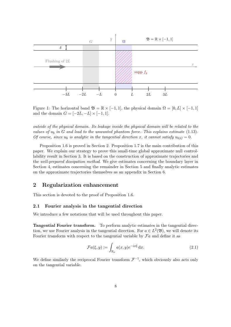
domain Ω will prove Theorem 1. We also introduce a domain

G := [−2L,−L]× [−1, 1] (see Fig. 1). (1.8)

We will denote by ex and ey the unit vectors of the canonical basis of R2.

Proposition 1.6 (Analytic regularization of the initial data). Let T > 0 and ρb > 0. Letu∗ ∈ L2

div(Ω) with∫

Ω u∗ · ex = 0. For any k ∈ N and ηb > 0, there exists an extensionua ∈ L2

div(B) of u∗ to the band B, a control force fc ∈ C∞([0, T ] × (B \ Ω)), a phantomforce fg ∈ C∞([0, T ]× Ω) satisfying

‖fg‖L1((0,T );Hk(Ω)) ≤ ηb, (1.9)

a weak Leray solution u ∈ C0([0, T ];L2div(B)) ∩ L2((0, T );H1(B)) to (1.7) associated with

the initial data ua, Cb > 0 and Tb ≤ T such that ub := u(Tb) ∈ L2div(B) satisfies

‖ub|G‖Hk(G) + ‖ub|B\Ω‖L2(B\Ω) + ‖ub|Ω − u∗‖L2(Ω) ≤ ηb, (1.10)

∀m ≥ 0, ‖∂mx ub‖H3(B) ≤m!

ρmbCb, (1.11)∑

0≤α+β≤3

‖∂αx ∂βy ub‖L1x(L2

y) ≤ Cb. (1.12)

Proposition 1.7 (Global approximate null controllability from any analytic initial data).Let T > 0. There exists ρb > 0 such that, for every σ > 0 and each ub ∈ L2

div(B) for whichthere exists Cb > 0 such that (1.11) and (1.12) hold, for every k ∈ N and δ ∈ (0, 1

2), thereexist two forces fc ∈ C∞([0, T ]× (B \ Ω)) and fg ∈ C∞([0, T ]× Ω) satisfying

‖fg‖L1((0,T );Hk(Ω)) ≤ Ck,δ‖ub|G‖Hk(G), (1.13)

supp fg ⊂ (0, T )× [0, L]× [−1 + δ, 1− δ], (1.14)supp fc ⊂ (0, T )×B \ Ω (1.15)

and a weak solution u ∈ C0([0, T ];L2loc,div(B)) ∩ L2((0, T );H1

loc(B)) to (1.7) associatedwith the initial data ub, such that there exists Tc ≤ T such that uc := u(Tc) ∈ L2

loc,div(B)satisfies

‖uc|Ω‖L2(Ω) ≤ σ + ‖ub||y|≥1−2δ‖L2(B). (1.16)

Moreover, the constant Ck,δ only depends on k and δ.

Proposition 1.8 (Local null controllability). Let T > 0. There exists σ > 0 such that,for any uc ∈ L2

div(Ω) which satisfies

‖uc|Ω‖L2(B) ≤ 3σ, (1.17)

there exists a weak solution u ∈ C0([0, T ];L2div(Ω)) ∩ L2((0, T );H1(Ω)) to (1.1) with the

initial data uc and fg = 0, which satisfies u(T ) = 0.

Proposition 1.8 is a direct consequence of known results concerning the small-time localnull controllability of the Navier-Stokes equation (see Remark 1.2 for references).

6

Let us prove that the combination of these three propositions implies Theorem 1. First,thanks to standard arguments, it is sufficient to prove Theorem 1 for initial data satisfying∫

Ω u∗ · ex = 0. Indeed, applying vanishing boundary controls on the original system forany positive time guarantees that the state gains this property. Therefore, we assume thatthe initial data already satisfies this property. We fix the quantities step by step in thefollowing manner.

• Let T > 0 and u∗ ∈ L2div(Ω) satisfying

∫Ω u∗ · ex = 0.

• Let ρb > 0 be given by Proposition 1.7 for a time interval of length T/3.

• Let σ > 0 be given by Proposition 1.8 for a time interval of length T/3.

• Let δ1 ∈ (0, 12) small enough such that ‖(u∗)||y|≥1−2δ1‖L2(Ω) ≤ σ.

• Let k ∈ N and η > 0.

• Let ηb := minη/2, σ, η/(2Ck,δ1).

• We apply Proposition 1.6 with a time interval of length T/3, ρb, k and ηb. Hence,there exists Tb ≤ T/3 and a solution u defined on [0, Tb] with u(0)|Ω = u∗ and suchthat ub := u(Tb) satisfies (1.10), (1.11) and (1.12).

• We apply Proposition 1.7 with a time interval of length T/3, ρb, δ1, k and σ. Thisyields a solution u defined on [Tb, Tc] with Tc ≤ Tb+T/3 ≤ 2T/3 such that uc := u(Tc)satisfies (1.16).

• By triangular inequality, ‖ub||y|≥1−2δ1‖L2(B) ≤ ‖ub|B\Ω‖L2(B) + ‖ub|Ω − u∗‖L2(Ω) +‖(u∗)||y|≥1−2δ1‖L2(Ω). Since ηb ≤ σ, (1.10) and (1.16) imply that (1.17) holds.

• Finally, we apply Proposition 1.8. This yields a solution u defined on [Tc, T3] withT3 := Tc + T/3 ≤ T such that u(T3) = 0.

• The concatenated forces fc and fg are C∞ by parts in time with C∞ regularity inspace.

• This concludes the proof of Theorem 1 up to extending the solution and the forcesby 0 on [T3, T ].

Remark 1.9. The fact that, starting from a finite energy initial data, the solution tothe Navier-Stokes equation instantly becomes analytic is well-known. However, in the un-controlled setting, the analytic radius only grows like

√t. In Proposition 1.6, we use the

phantom force to enhance the regularization in short time.

Remark 1.10. The small-time global approximate null controllability result of Proposi-tion 1.7 will be proved thanks to a return-method argument (see Section 3). A base flowwill shift the whole band B of a distance 2L towards the right. Roughly speaking, the mainpart of the initial data ub|Ω will then be outside of the physical domain and killed by acontrol force. However, since we need to work in an analytic setting (to establish estimatesfor a PDE with a derivative loss, see Section 5), this action cannot be exactly localized

7

x

y

0 L 2L 3L−L−2L−3L

Flushing of 2L

δ

B = R× [−1, 1]ΩG

supp fg

Figure 1: The horizontal band B = R × [−1, 1], the physical domain Ω = [0, L] × [−1, 1]and the domain G = [−2L,−L]× [−1, 1].

outside of the physical domain. Its leakage inside the physical domain will be related to thevalues of ub in G and lead to the unwanted phantom force. This explains estimate (1.13).Of course, since ub is analytic in the tangential direction x, it cannot satisfy ub|G = 0.

Proposition 1.6 is proved in Section 2. Proposition 1.7 is the main contribution of thispaper. We explain our strategy to prove this small-time global approximate null control-lability result in Section 3. It is based on the construction of approximate trajectories andthe well-prepared dissipation method. We give estimates concerning the boundary layer inSection 4, estimates concerning the remainder in Section 5 and finally analytic estimateson the approximate trajectories themselves as an appendix in Section 6.

2 Regularization enhancement

This section is devoted to the proof of Proposition 1.6.

2.1 Fourier analysis in the tangential direction

We introduce a few notations that will be used throughout this paper.

Tangential Fourier transform. To perform analytic estimates in the tangential direc-tion, we use Fourier analysis in the tangential direction. For a ∈ L2(B), we will denote itsFourier transform with respect to the tangential variable by Fa and define it as

Fa(ξ, y) :=

∫Rxa(x, y)e−ixξ dx. (2.1)

We define similarly the reciprocal Fourier transform F−1, which obviously also acts onlyon the tangential variable.

8

Band-limited functions. Let N > 0. We will sometimes need to consider functionsin L2(B) whose Fourier transform is supported within the set of tangential frequencies ξsatisfying |ξ| ≤ N . Therefore, we introduce the Fourier multiplier

PN (ξ) := 1[−N,N ](ξ) (2.2)

and the associated functional space

L2N (B) :=

a ∈ L2(B); a = PNa

. (2.3)

For any k ∈ N and a ∈ Hk(B), it is clear that

‖PNa− a‖Hk(B) → 0 as N → +∞. (2.4)

2.2 Regularization enhancement using the phantom and the control

We start with the following lemma concerning the possibility to remove high tangentialfrequencies from a smooth initial data. We denote by P the usual Leray projector ondivergence free vector fields, tangent to ∂B.

Lemma 2.1. Let ua ∈ L2div(B) and Tb > 0. We denote by ua the solution of the free

Navier-Stokes equation at time Tb starting from ua. There exists a family indexed byN > 0 of vector fields uN ∈ C0([0, Tb];L

2div(B))∩L2((0, Tb);H

1(B)) associated with forcesfN ∈ C0([0, Tb];H

k(B)), which are weak Leray solutions to

∂tuN −∆uN + P[(uN · ∇)uN ] = PfN , uN (0) = ua (2.5)

and satisfy, for any k ∈ N and ρb > 0,

‖(fN )|Ω‖L1((0,Tb);Hk(Ω)) −→N→+∞

0, (2.6)

fN ∈ C∞([0, Tb]×B), (2.7)‖(uN (Tb)− ua)|Ω‖L2(Ω) −→

N→+∞0, (2.8)

‖(uN (Tb))|G‖Hk(G) −→N→+∞

0, (2.9)

‖(uN (Tb))|B\Ω‖L2(B\Ω) ≤ ‖(ua)|B\Ω‖L2(B\Ω) + oN→+∞

(1), (2.10)

∃CN > 0, supm≥0‖∂mx uN (Tb)‖H3(B) ≤

m!

ρmbCN , (2.11)

∃CN > 0,∑

0≤α+β≤3

‖∂αx ∂βy uN (Tb)‖L1x(L2

y) ≤ CN . (2.12)

Proof. Let ua ∈ L2div(B). Let Tb > 0. Let v be the weak Leray solution to

∂tv −∆v + P[(v · ∇)v] = 0, v(0) = ua. (2.13)

Hence, by definition, ua = v(Tb). It is classical to prove that v ∈ C∞((0, Tb] × B) (seee.g. [34]). Let β ∈ C∞([0, Tb]; [0, 1]) with β = 1 on [0, Tb/3] and β = 0 on [2Tb/3, Tb]. Let

9

θ ∈ C∞(B; [0, 1]) with θ = 1 for x ∈ [0, L] and θ = 0 for x < −L or x > 2L. We consideru := βv + (1− β)θv. Then, u is the weak Leray solution to

∂tu−∆u+ P[(u · ∇)u] = Pg, u(0) = ua, (2.14)

where we set

g := β(1− θ)v − 2(1− β)(∇θ · ∇)v − (1− β)∆θv

− β(1− β)(v · ∇)((1− θ)v)− (1− β)2(θv · ∇)((1− θ)v).(2.15)

Hence, supp g ⊂ [Tb/3, Tb]× (B \ Ω) and g ∈ C∞([0, Tb]×B). We define

uN (t) := β(t)u(t) + (1− β(t))PNu(t), (2.16)

where PN is defined in (2.2). In particular, (2.16) implies (2.5), provided that one sets

fN := β(u−PNu) + (1− β)(

(PNu · ∇)PNu−PN ((u · ∇)u))

+ β(1− β)(

(u · ∇)(PNu− u)− (PNu · ∇)(PNu− u))

+ βg + (1− β)PNg.

(2.17)

Let k ∈ N. Thanks to definition (2.17), there holds (2.6) and (2.7). Indeed, u belongsto C0([Tb/3, Tb];H

k+1(Ω)) and the family PNu converges towards u in this space. From(2.16), at the final time, one has

uN (Tb) = PNu(Tb) = PN (θv(Tb)) = PN (θua). (2.18)

In particular, we deduce from (2.18) that uN (Tb) is "entire" in x so that, for any ρb > 0,there exists Cb > 0 such that (2.11) holds. We also deduce from (2.18) that uN (Tb)→ θuain Hk(B), which implies (2.8), (2.9) and (2.10).

To obtain (2.12), we change slightly the definition (2.2) of PN . Instead of a rectangularwindow filter, we define PN as the Fourier multiplier WN , where WN ∈ C∞(R; [0, 1]) issuch thatWN (ξ) = 1 for ξ ∈ [−N+1, N−1] andWN (ξ) = 0 when |ξ| ≥ N . This preservesthe property (2.4) but has a better behavior with respect to L1 norms in space. Indeed,if φ ∈ S(R,R), one checks that WNφ ∈ L1(R). This property implies (2.12) becauseu(Tb) = θv(Tb) has a compact support.

2.3 Proof of the regularization proposition

We turn to the proof of Proposition 1.6.Let T, ρb, ηb > 0 and k ∈ N. Let u∗ ∈ L2

div(Ω) satisfying∫

Ω u∗ · ex = 0. We start byextending u∗ into ua ∈ L2

div(B) such that ‖(ua)|B\Ω‖L2(B\Ω) ≤ ηb/10. For Tb ∈ (0, T ) smallenough, the free solution starting from ua at time Tb, say ua satisfies ‖(ua)|B\Ω‖L2(B\Ω) ≤ηb/5 and ‖(ua)|Ω − u∗‖L2(Ω) ≤ ηb/5.

We choose N large enough such that (2.8), (2.9) and (2.10) imply that ub := uN (Tb),where the family (uN , fN ) is given by Lemma 2.1, satisfies (1.10) and such that (2.6)ensures (1.9). Estimates (2.11) and (2.12) prove (1.11) and (1.12). This concludes theproof of Proposition 1.6, provided that we define fg := (fN )|Ω and fc := (fN )|B\Ω, eachbeing smooth within its support.

10

3 Strategy for global approximate controllability

We explain our strategy to prove Proposition 1.7. Let T > 0, ub ∈ L2div(B), δ ∈ (0, 1

2) andk ∈ N. We intend to construct a family of approximate trajectories depending on a smallparameter 0 < ε 1 and driving ub approximately to zero. We detail the constructionof this family in the following paragraphs. Then, we prove estimates on boundary layerterms for these approximate trajectories in Section 4. We prove estimates on the remainderin Section 5 and postpone analytic-type estimates for these approximate trajectories toSection 6.

3.1 Small-time to small-viscosity scaling

Let κ ∈ (0, 1). Although it might seem like a further complication, our strategy is basedon trying to control the system (1.7) at an even shorter time scale, ε1−κT , passing throughintermediate states (velocities) of order 1/ε. For ε ∈ (0, 1), we introduce the trajectories

U ε(t, x, y) := uε(t/ε, x, y)/ε, P ε(t, x, y) := pε(t/ε, x, y)/ε2, (3.1)

F εg (t, x, y) := f εg (t/ε, x, y)/ε2 and F εc (t, x, y) := f εc (t/ε, x, y)/ε2. (3.2)

The tuples (U ε, P ε, F εc , Fεg ) define solutions to (1.7) with initial data ub if and only if the

new unknowns (uε, pε, fεc , fεg ) are solutions to the rescaled system

∂tuε + (uε · ∇)uε +∇pε − ε∆uε = f εg + f εc in (0, T/εκ)×B,

div uε = 0 in (0, T/εκ)×B,

uε = 0 on (0, T/εκ)× ∂B,uε|t=0 = εub in B.

(3.3)

Observe the three differences between (3.3) and the original system (1.7):

• the Laplace term has a small factor ε in front of it rather than 1,

• the system is set on the long time interval (0, T/εκ) rather than (0, T ),

• the initial data is εub rather than ub.

We construct approximate solutions to (3.3) in the following paragraph.

3.2 Return method ansatz

We introduce the following explicit approximate solution to (3.3):

uεapp(t, x, y) := u0(t) + χ(y)v0(t, ϕ(y)/

√ε)

+ εu1(t, x, y)+ε2wε(t, y), (3.4)

pεapp(t, x, y) := p0(t, x), (3.5)

f εc (t, x, y) := εf1|B\Ω(t, x, y), (3.6)

f εg (t, x, y) := εf1|Ω(t, x, y). (3.7)

In the following lines, we define each of the three terms involved in this approximatesolution. We refer to Section 3.4 for comments on the choice of these profiles.

11

Base Euler flow profile. Let n ∈ N satisfying n ≥ 3 and

n >3

4

(1

κ− 1

). (3.8)

Let h in C∞(R+,R) be such that

supp h ⊂ (0, T/3] ∪ [2T/3, T ), (3.9)∫ T/3

0h(t)dt = 2L, (3.10)∫ T

0tkh(t)dt = 0 for 0 ≤ k < n. (3.11)

We defineu0(t) := h(t)ex and p0(t, x) := −h(t)x. (3.12)

For a function a ∈ L2(B), we will denote its translation along the base flow h by

(τha)(t, x, y) := a

(x−

∫ t

0h(s) ds, y

). (3.13)

Boundary layer profile. Let ϕ ∈ C∞([−1, 1], [0, 1]) such that ϕ(±1) = 0 and |ϕ′(y)| =1 for |y| ≥ 1/4. Let χ ∈ C∞([−1, 1], [0, 1]) such that χ(y) = 1 for |y| ≥ 2/3, and χ(y) = 0for |y| ≤ 1/3. Let V (t, z) be the solution to

∂tV − ∂zzV = 0 in R+ × R+,

V (t, 0) = h(t) on R+,

V (0, z) = 0 in R+.

(3.14)

We definev0(t, z) := −V (t, z)ex. (3.15)

In the sequel, for any function V(t, z), depending on the fast variable, we will denote itsevaluation at z = ϕ(y)/

√ε by

V(t, y) := V(t,ϕ(y)√ε

). (3.16)

Linearized Euler flow profile. Let β ∈ C∞(R+, [0, 1]) non-increasing such that β(t) =1 for t ≤ T/3 and β(t) = 0 for t ≥ 2T/3. Let χδ ∈ C∞([−1, 1], [0, 1]) such that χδ(y) = 1for |y| ≤ 1 − 2δ and χδ(y) = 0 for |y| ≥ 1 − δ. We define the stream function associatedwith ub, then u1 and eventually the force f1.

ψb(x, y) := −∫ y

−1ub(x, y

′) · ex dy′, (3.17)

u1(t, x, y) := β(t)τh∇⊥[χδψb] + τh∇⊥[(1− χδ)ψb], (3.18)

f1(t, x, y) := β(t)(χδ(y)ub(x− 2L, y)− χ′δ(y)ψb(x− 2L, y)ex

). (3.19)

12

Technical profile. For t ∈ R+ and y ∈ [−1, 1], we define the source

f εW :=χ′′

ϕ4z4V + 2

χ′

ϕ5ϕ′z5∂zV . (3.20)

Let W ε(t, y) : R+ × [−1, 1]→ R be the solution to∂tW

ε − ε∂yyW ε = f εW in R+ × [−1, 1],

W ε(t,±1) = 0 on R+,

W ε(0, y) = 0 in [−1, 1].

(3.21)

Finally, we letwε(t, y) := W ε(t, y)ex. (3.22)

Equation satisfied by the approximate trajectories. Then (uεapp, pεapp) are solutions

to∂tu

εapp +

(uεapp · ∇

)uεapp − ε∆uεapp +∇pεapp = f εc + f εg + εf εapp in (0, T/εκ)×B,

div uεapp = 0 in (0, T/εκ)×B,

uεapp = 0 on (0, T/εκ)× ∂B,uεapp|t=0 = εub in B,

(3.23)where we define

f εapp :=− ε∆u1 + ε(u1 · ∇)u1+ε2W ε∂xu1 + ε2(u1 · ey)∂ywε

− χV ∂xu1 − u1 · eyϕ

(√εχ′zV + χϕ′z∂zV

)ex.

(3.24)

3.3 Estimates and proof of approximate controllability

By construction, the approximate trajectory will be small at the final time.

Proposition 3.1. There exists a constant Capp > 0 such that, for ε > 0 small enough,

1

ε‖uεapp(T/εκ)|Ω‖L2(B)

≤ Capp

(ε

14 + εκ(n− 3

4( 1κ−1))| ln ε|n+ 3

4

)+ ‖ub||y|≥1−2δ‖L2(B).

(3.25)

Moreover, the approximate trajectory can be arbitrarily close to a true trajectory.Indeed, we can construct a remainder which is small, provided that the initial data ub issufficiently regular (its tangential analytic radius is large enough).

Proposition 3.2. There exists ρb > 0, depending only on T such that, if ub satisfies (1.11)and (1.12) for some Cb > 0, there exists Cr > 0 such that, for ε > 0 small enough, there

13

exists a weak Leray solution rε ∈ C0([0, T/εκ], L2div(B)) ∩ L2((0, T/εκ), H1(B)) to

∂trε +

(uεapp · ∇

)rε + ε (rε · ∇) rε + (rε · ∇)uεapp

−ε∆rε +∇πε = −f εapp in (0, T/εκ)×B,

div rε = 0 in (0, T/εκ)×B,

rε = 0 on (0, T/εκ)× ∂B,rε|t=0 = 0 in B,

(3.26)which moreover satisfies

‖rε‖L∞((0,T/εκ);L2(B)) ≤ Cr(ε14 + ε1−κ). (3.27)

It is straightforward to check that Proposition 3.1 and Proposition 3.2 imply Proposi-tion 1.7. Indeed, let ρb be given by Proposition 3.2 and assume that ub satisfies (1.11) and(1.12) for some Cb > 0. We choose ε > 0 small enough such that the conclusions of bothpropositions hold. We construct an exact trajectory by setting

uε := uεapp + εrε and pε := pεapp + επε. (3.28)

Combining (3.28) with the equation (3.23) satisfied by uεapp and the equation (3.26) satisfiedby rε proves that uε is a weak solution to (3.3).

Let σ > 0. Choosing ε > 0 small enough, summing estimates (3.25) and (3.27) andrecalling the definition (3.28) of uε, the assumption (3.8) on n and the scaling (3.1) provesthat (1.16) holds at the time Tc := ε1−κT < T .

Since ub satisfies (1.11), ub ∈ C∞(B). Thus, thanks to (3.2), (3.6), (3.7) and (3.19),Fg ∈ C∞([0, Tc]× Ω), Fc ∈ C∞([0, Tc]×B \ Ω) and moreover

suppFg ⊂ (0, Tc)× [0, L]× [−1 + δ, 1− δ], (3.29)suppFc ⊂ (0, Tc)×B \ Ω, (3.30)

Moreover, using (3.2), (3.7) and (3.19), one has

‖F εg (t)‖L1([0,Tc];Hk(Ω)) =1

ε2‖f εg (t/ε)‖L1([0,ε1−κT ];Hk(Ω))

=1

ε‖f εg (t)‖L1([0,T/εκ];Hk(Ω))

= ‖f1|Ω‖L1([0,T/εκ];Hk(Ω))

= ‖χδub + χ′δψb‖Hk(G),

(3.31)

where we recall that the set G is defined in (1.8). This proves the estimate (1.13) concerningthe size of the phantom force, for a constant Ck,δ which only depends on the norm of χδin Hk+1(−1, 1), and thus concludes the proof of the approximate controllability resultProposition 1.7.

We prove Proposition 3.1 in Section 4 (thanks to the well-prepared dissipation method)and Proposition 3.2 in Section 5 (using a long-time nonlinear Cauchy-Kovalevskaya esti-mate).

14

3.4 Comments and insights on the proposed expansion

Remark 3.3 (Return method and base Euler flow). Since system (3.3) can be seen as aperturbation of the Euler equations a natural idea is to follow the return method introducedby Coron in [5] (see also [7, Chapter 6]) to prove the controllability of the Euler equationsin the 2D case (see also [6], and [16] for the 3D case). Loosely speaking the idea is toovercome that the linearized problem around zero is not controllable by introducing, thanksto the boundary control, a velocity u0 of order O(1) (whereas the initial velocity is only oforder O(ε)) solution to the Euler equation satisfying u0|t=0 = u0|t=T = 0 and such that thecorresponding flow flushes all the domain out during the time interval (0, T ). In the presentcase of a rectangle this step is pretty easy and explicit: it corresponds to the introductionof a flow which flushes out the initial data. From (3.12), we get that (u0, p0) indeed solvesthe incompressible Euler equation:

∂tu0 +

(u0 · ∇

)u0 = −∇p0, in R+ ×B,

div u0 = 0 in R+ ×B,

u0 · ey = 0 on R+ × ∂B,(3.32)

with initial data u0(0) = 0 and u0(t) = 0 for t ≥ T .

Remark 3.4 (Transport of the initial data). The term u1 takes into account the initialdata ub, which is transported by the flow u0. Using (3.12), (3.18) and (3.19), we obtainthat u1 solves

∂tu1 + h(t)∂xu

1 = f1 in R+ ×B,

div u1 = 0 in R+ ×B,

u1 = 0 on R+ × ∂B,u1(0) = ub in B.

(3.33)

Thanks to assumption (3.10), it is clear that the initial data will be flushed outside of thedomain at time T/3. During the time interval [T/3, 2T/3], the initial data ub has beenshifted towards the right of a distance 2L. This is the time interval during which the forcef1 kills most of the initial data (for |y| ≤ 1− δ).

The key point is that, outside of the physical domain, this force is merely a control.However, since we need this force to be analytic, it also acts a little bit within the physicaldomain. This gives rise to an unwanted phantom force.

Remark 3.5 (Boundary layer correction). A major difficulty is linked to the discrepancybetween the Euler and the Navier-Stokes equations in the vanishing viscosity limit. Indeed,although inertial forces prevail inside the domain, viscous forces play a crucial role nearthe uncontrolled boundary, and give rise to a boundary layer of order O(1) associated withthe velocity u0 which does not satisfy the tangential part of the Dirichlet condition on thetop and bottom boundaries.

The purpose of the second term v0 is to recover the Dirichlet boundary condition byintroducing the boundary layer generated by u0. Thanks to our previous choice of u0 we willavoid the difficulty usually associated with the Prandtl equation. Indeed the boundary layerwill also be fully horizontal (tangential) and will not depend on x so that the equation forv0 will deplete into a linear heat equation with non-homogeneous Dirichlet data depending

15

on u0. The quantity ϕ(y)/√ε reflects quick variations within the boundary layer, where

ϕ(y) is the distance to the boundary.

4 Well-prepared dissipation method for the boundary layer

The key argument of the well-prepared dissipation method is that the normal dissipationinvolved in fluid mechanics boundary layer equations can dissipate most of their energy,provided that the created boundary layers are “well-prepared” in some sense. Roughlyspeaking, this preparation amounts to ensure that they do not contain energy at lowfrequencies.

4.1 Large time decay of the boundary layer profile

In the work [9] concerning the case of the Navier slip-with-friction boundary condition, weused boundary controls to import enough vanishing moments thanks to the transport bythe Euler flow within the boundary layer. In this work, we cannot use this strategy becausewe do not want the boundary layer profile to depend on the slow tangential variable, seeRemark 3.5. Instead we rely on the assumptions (3.11) on the base Euler flow. We provebelow that these conditions entail a good decay for the boundary layer profile. This decaywill be used both to prove that the source terms generated by v in equation (3.26) for theremainder are integrable with respect to time and that the boundary profile at the finaltime is small enough to apply a local controllability result. For s,m ∈ N and I an intervalof R, we introduce the following weighted Sobolev spaces:

Hs,m(I) :=

f ∈ Hs(I),

s∑α=0

∫I

(1 + z2

)m ∣∣∣f (α)(z)∣∣∣2 dz < +∞

, (4.1)

which we endow with their natural norm. We will use this definition with I = R or I = R+.

Lemma 4.1. Let T > 0, s, n ∈ N and h ∈ C∞(R,R) satisfying (3.9) and (3.11). Weconsider V the solution to (3.14). For any 0 ≤ m ≤ 2n+ 1, there exists a constant C suchthat the following estimate holds:

|V (t, ·)|Hs,m(R+) ≤ C∣∣∣∣ ln(2 + t)

2 + t

∣∣∣∣ 14+ 2n+12−m

2

. (4.2)

Proof. Estimate (4.2) is straightforward up to time T because its right-hand side is boundedfrom below for t ∈ [0, T ]. Thus, we focus on large time estimates. We start by explicitcomputations in the frequency domain using Fourier transform. We consider the auxiliarysystem

∂tf − ∂zzf = (h(t)− h(t)) · sgn(z)e−|z|, t ≥ 0, z ∈ R,f(0, z) = 0, t = 0, z ∈ R.

(4.3)

Since the source term in (4.3) is odd, its unique solution f satisfies f(t, 0) = 0 for allt ∈ R+. Hence, thanks to the uniqueness property for the heat equation on the half-line,there holds V (t, z) = f(t, z) + h(t)e−z for t, z ≥ 0 because both sides of this equality solve

16

the same heat equation. Therefore, proving estimates on f will provide estimates on V .After Fourier transform and solving the ODE, we obtain the formula:

f(t, ζ) :=

∫Rf(t, z)e−iζzdz = − 2iζ

1 + ζ2

∫ t

0e−(t−s)ζ2

(h(s)− h(s)

)ds. (4.4)

Since h vanishes after T (see (3.9)), the behavior of f (and thus V ) after time T is en-tirely determined by the “initial” data fT (z) := f(T, z). Thanks to [9, Lemma 6], toestablish (4.2), it suffices to check that, for 0 ≤ j ≤ 2n,

∂jζ fT (0) = 0. (4.5)

Thanks to (4.4) and to the Leibniz rule, for j ∈ N, one has:

∂jζ fT (ζ) = −ij∑

k=0

(j

k

)∂j−kζ

2ζ

1 + ζ2

∫ T

0

(h(t)− h(t)

)∂kζ

e−(T−t)ζ2

dt. (4.6)

First, since ζ 7→ 2ζ/(1 + ζ2) is an odd function, only its odd derivatives don’t vanish atzero. Second, thanks to the Arbogast rule for the iterated differentiation of compositefunctions (also known as Faà di Bruno’s formula), one has:

∂kζ

e−(T−t)ζ2

=

∑m1+2m2=k

k!

m1!m2!

(−2ζ(T − t)1!

)m1(−2(T − t)

2!

)m2

e−(T−t)ζ2 . (4.7)

Hence, this derivative is non null at zero only if k is even, say k = 2k′ and the only non-vanishing term in the right-hand side of (4.7) is the one corresponding to (m1,m2) = (0, k′)and is proportional to (T − t)k′ . From (4.6) and (4.7) we deduce that ∂jζ fT (0) is a linearcombination of the moments ∫ T

0

(h(t)− h(t)

)(T − t)k′dt, (4.8)

where 0 ≤ 2k′ ≤ j−1. Thanks to (3.9) and (3.11), the integrals (4.8) vanish for 0 ≤ k′ < n.So (4.5) holds for j ≤ 2n− 1. Last, (4.5) also holds for j = 2n because, when j is even, allthe terms vanish. Indeed, in (4.6), either k is odd or j−k = 2n−k is even. This concludesthe proof of the lemma.

4.2 Fast variable scaling and Lebesgue norms

Let us prove the following lemma, which is a simpler version of [19, Lemma 3, page 150].

Lemma 4.2. Let γ ∈ C0([−1, 1]) with γ ≡ 0 on(−1

3 ,13

). For V ∈ L2(R+) and ε > 0:

‖γV‖L2(−1,1) ≤ 2ε14 ‖γ‖∞‖V‖L2(R+). (4.9)

Proof. For −1 ≤ y ≤ −14 , we assumed ϕ′ = 1. Thus, ϕ(y) = 1 + y. Recalling the fast

variable notation (3.16) and performing an affine change of variables gives∫ − 13

−1γ2(y)V2

(ϕ(y)√ε

)dy =

√ε

∫ 23√ε

0γ2(√εz − 1)V2(z) dz ≤ √ε‖γ‖2∞‖V‖2L2(R+). (4.10)

Proceeding likewise for 13 ≤ y ≤ 1 and bounding

√2 by 2 yields (4.9),

17

4.3 Estimates for the technical profile

Lemma 4.3. Assume that (3.11) holds for some n ≥ 3. There exists CW such that, forevery ε ∈ (0, 1), the solution W ε to (3.21) satisfies, for every t ≥ 0,

‖W ε(t)‖L∞(−1,1) + ‖∂yW ε(t)‖L∞(−1,1) ≤ ε−34CW . (4.11)

Proof. Differentiating (3.21) with respect to time, multiplying by ∂tW ε and integrating byparts, we obtain the energy estimate

‖∂tW ε‖L∞(R+;L2(−1,1)) ≤ 2‖∂tf εW ‖L1(R+;L2(−1,1)). (4.12)

Plugging this estimate in the equation (3.21) yields

‖∂yyW ε‖L∞(R+;L2(−1,1)) ≤1

ε

(‖f εW ‖L∞(R+;L2(−1,1)) + 2‖∂tf εW ‖L1(R+;L2(−1,1))

), (4.13)

Thanks to estimate (4.9) from Lemma 4.2 applied to the definition (3.20) of f εW , we obtain,for t ≥ 0,

‖f εW (t)‖L2(−1,1) ≤ 2ε14 ‖χ′′/ϕ4‖∞‖z4V (t, z)‖L2(R+)

+ 2ε14 ‖2χ′ϕ′/ϕ5‖∞‖z5∂zV (t, z)‖L2(R+)

≤ Cε 14 ‖V (t)‖H1,5(R+),

(4.14)

where C is a finite constant because, by construction, χ′ and χ′′ vanish for |y| ≥ 23 , so that

the division by ϕ which vanishes at y = ±1 is not singular. Proceeding similarly and usingthe equation (3.14) on V , we obtain

‖∂tf εW (t)‖L2(−1,1) ≤ Cε14 ‖V (t)‖H3,5(R+). (4.15)

Combining (4.14) with Lemma 4.1 applied to m = 5, n = 3, s = 1, we obtain

‖f εW (t)‖L2(−1,1) ≤ Cε14

∣∣∣∣ ln(2 + t)

2 + t

∣∣∣∣ 54 ≤ Cε 14 (4.16)

Combining (4.15) with Lemma 4.1 applied to m = 5, n = 3, s = 3, we obtain

‖∂tf εW ‖L1(R+;L2(−1,1)) ≤ Cε14

∫ +∞

0

∣∣∣∣ ln(2 + t)

2 + t

∣∣∣∣ 54 dt ≤ 26Cε14 . (4.17)

Eventually, plugging (4.16) and (4.17) into (4.13) proves (4.11) thanks to the boundaryconditions W ε(t,±1) = 0 and the Poincaré-Wirtinger inequality for ∂yW ε.

4.4 Proof of the decay of approximate trajectories

We prove Proposition 3.1. Recalling the definition (3.4) of uεapp, we estimate the size ofeach term at the time T/εκ.

• Thanks to (3.9) and (3.12), u0(T/εκ) = 0.

18

• Thanks to (4.9) from Lemma 4.2 and (4.2) from Lemma 4.1, there holds

‖χv0(T/εκ)‖L2y≤ 2ε

14 ‖χ‖∞‖V (T/εκ)‖L2(R+)

≤ 2ε14C

∣∣∣∣ ln(2 + T/εκ)

2 + T/εκ

∣∣∣∣ 34+n

≤ Cε1+κ(n− 34

( 1κ−1))| ln ε|n+ 3

4 ,

. (4.18)

for some constant C > 0.

• Thanks to (3.18),u1(T/εκ) = ∇⊥[(1− χδ)ψb]. (4.19)

Moreover, since ub satisfies (1.12), ub ∈ L1(B). In particular, since ub is divergence-free, this implies that, for all x ∈ R,∫ +1

−1ub(x, y) · ex dy = 0, (4.20)

so that ψb, which was defined as (3.17) can equivalently be written as

ψb(x, y) =

∫ 1

yub · ex dy. (4.21)

Thanks to (4.19), this implies that there exists a constant Cδ > 0 which only dependson the norm of χδ in H1(−1, 1) such that

ε‖u1(T/εκ)‖L2(B) ≤ εCδ‖ub||y|≥1−2δ‖L2(B). (4.22)

• Thanks to estimate (4.11) from Lemma 4.3,

ε2‖wε(T/εκ)‖L∞y ≤ ε1+ 14CW . (4.23)

Gathering these estimates concludes the proof of estimate (3.25) of Proposition 3.1.

5 Estimates on the remainder

This section is devoted to the proof of Proposition 3.2. An important difficulty to obtainsome uniform energy estimates of rε from system (3.26) is that the term (rε · ∇)uεapp

contains a term with a factor 1/√ε due to the fast variation of the boundary layer term in

the normal variable (see the expansion (3.4) of uεapp). To deal with this difficulty we use areformulation of this term where the singular factor is traded against a loss of derivative onrε in the tangential direction x (see Section 5.1). Then, we establish a long-time nonlinearCauchy-Kovalevskaya estimate (see Section 5.3) thanks to some tools from Littlewood-Paley theory which are recalled in Section 5.2.

Remark 5.1. The well-posedness of the Prandtl equations as well as the convergence ofthe Navier-Stokes equations to the Prandtl equations in the analytic setting dates back to[32, 33, 27]. The seminal results of Caflisch and Sammartino require analyticity in bothspatial directions, and only imply well-posedness of the Prandtl equations on a small timeinterval. Analytic techniques have been later used in [20, 35] to obtain large-time well-posedness for Prandtl equations by requiring analyticity only in the tangential direction.

19

5.1 Singular amplification to loss of derivative

On the one hand, we use the expansion (3.4) of uεapp to expand

(rε · ∇)uεapp =1√εϕ′χrε2∂zv0+ rε2(χ′v0+ε2∂yw

ε) + ε (rε · ∇)u1. (5.1)

Let M be the operator which associates with any function a ∈ L2(−1, 1), the functionM [a] defined for y in (−1, 1) by

(M [a])(y) := −χ(y)

∫ 1

0a(±1∓ s(1∓ y)) ds, (5.2)

where the signs are chosen depending on whether ±y ≥ 0. Using the null boundarycondition and the divergence-free condition in (3.26) and the fact that |ϕ′| = 1 whereχ 6= 0, we obtain that the first term in the right-hand side of (5.1) can be recast as

1√εϕ′χrε2∂zv0 = (M [∂xr

ε1])z∂zv0. (5.3)

On the other hand we decompose the term (uεapp · ∇)rε of (3.26), thanks to (3.4), into(uεapp · ∇

)rε = (h− χV +ε2W ε)∂xr

ε + ε(u1 · ∇

)rε, (5.4)

Thus, using (5.3) and (5.4), the system (3.26) now reads∂tr

ε + (h− χV +ε2W ε)∂xrε − ε∆rε +∇πε = f εr in (0, T/εκ)×B,

div rε = 0 in (0, T/εκ)×B,

rε = 0 on (0, T/εκ)× ∂B,rε|t=0 = 0 on B,

(5.5)

where we introduce

−f εr := f εapp + (M [∂xrε1])z∂zv0+ rε2(χ′v0+ε2∂yw

ε)

+ ε (rε · ∇)u1 + ε(u1 · ∇

)rε + ε (rε · ∇) rε.

(5.6)

5.2 A few tools from Littlewood-Paley theory

To perform analytic estimates, we use Fourier analysis and Littlewood-Paley decomposi-tion. We refer to [1, Chapter 2] for a detailed course on Littlewood-Paley theory. Althoughall the functions we consider in this section are defined on the band B = Rx × [−1, 1]y,we only perform Fourier analysis and Littlewood-Paley decomposition in the tangentialdirection x ∈ Rx. When a confusion is possible, we will use the subscripts x or y to stressthe variable involved in the functional spaces.

20

Dyadic partition of unity. We recall that, for a ∈ L2(B), we defined its Fouriertransform Fa in the tangential direction as (2.1). We fix χlp, ϕlp ∈ C∞(R, [0, 1]) such that

suppϕlp ⊂τ ∈ R;

3

4≤ |τ | ≤ 8

3

, (5.7)

suppχlp ⊂τ ∈ R; |τ | ≤ 4

3

, (5.8)

∀τ ∈ R∗,∑j∈Z

ϕlp(2−jτ) = 1, (5.9)

∀τ ∈ R, χlp(τ) +∑j∈N

ϕlp(2−jτ) = 1, (5.10)

∀τ ∈ R∗,1

2≤∑j∈Z

ϕ2lp(2−jτ) ≤ 1, (5.11)

The existence of such a dyadic partition of unity is proved in [1, Proposition 2.10]. Fork ∈ Z, we introduce the Fourier multipliers ∆k and Sk by defining, for any a ∈ L2(B),

∆ka := F−1(ϕlp(2−kξ)Fa(ξ, y)

), (5.12)

Ska := F−1(χlp(2−kξ)Fa(ξ, y)

). (5.13)

The operators ∆k and Sk are with respect to the horizontal variable only. For a ∈ L2(B),one has, thanks to (5.9) and (5.10),

Ska =∑j≤k−1

∆ja. (5.14)

Homogeneous Besov spaces. For a ∈ L2(B), we will use for s = 0 and s = 12 the

following quantity corresponding to a homogeneous Besov norm

‖a‖Bs :=∑k∈Z

2ks‖∆ka‖L2(B). (5.15)

Since we will use such norms for functions whose Fourier transforms in x are compactlysupported, we do not provide more details on the definition of the corresponding functionalspaces, referring for more to [1].

Classical estimates. We recall the following classical estimates, for which we track theconstants. First, we will use the following Bernstein type lemma from [1, Lemma 2.1].

Lemma 5.2. There exists a universal constant CB ≥ 2 such that the following propertieshold. Let 1 ≤ p ≤ q ≤ +∞, α ∈ 0, 1, k ∈ Z and a ∈ L2(B).

• If the support of Fa is included in (ξ, y); 2−k|ξ| ≤ 100, then

‖∂αx a‖Lqx(L2y) ≤ CB2

k(α+

(1p− 1q

))‖a‖Lpx(L2

y). (5.16)

21

• If the support of Fa is included in (ξ, y); 1100 ≤ 2−k|ξ| ≤ 100, then

‖a‖Lpx(L2y) ≤ CB2−kα‖∂αx a‖Lpx(L2

y). (5.17)

Lemma 5.3. Let a ∈ H10 ([−1, 1]y). Then

‖a‖L∞y ≤ ‖a‖12

L2y‖∂ya‖

12

L2y. (5.18)

Proof. This is a classical Gagliardo-Nirenberg interpolation inequality (see [30]). The factthat (5.18) holds with a unit constant for this particular choice of exponents is proved forexample in [29, Corollary 5.12] (which in fact yields a constant 2−

12 ).

As a consequence of Lemma 5.2, we have the following embedding. Indeed this is themain motivation for considering the `1 norm rather than the `2 norm in the definition ofthe homogeneous Besov norms Bs.

Lemma 5.4. Let a ∈ H10 (B). There holds,∑

k∈Z2k2 ‖∆ka‖L2

x(L∞y ) ≤ CB‖∇a‖B0 , (5.19)∑k∈Z‖∆ka‖L∞(B) ≤ C2

B‖∇a‖B0 . (5.20)

Proof. Let a ∈ H10 (B). Hence, for almost every x ∈ Rx, a(x, ·) ∈ H1

0 ([−1, 1]y) and we canapply Lemma 5.3. Using (5.18), Cauchy-Schwarz then (5.17) yields

2k2 ‖∆ka‖L2

x(L∞y ) ≤ 2k2 ‖∆ka‖

12

L2‖∆k∂ya‖12

L2

≤ C12B‖∆k∂xa‖

12

L2‖∆k∂ya‖12

L2

≤ C12B‖∆k∇a‖L2 ,

(5.21)

Hence, since CB ≥ 1, (5.21) proves (5.19) by the definition (5.15) of the norm B0. Moreover,thanks to (5.16),

‖∆ka‖L∞x (L∞y ) ≤ CB2k2 ‖∆ka‖L2

x(L∞y ). (5.22)

Gathering (5.19) and (5.22) proves (5.20).

Lemma 5.5. Let a ∈ H10 (B) such that div a = 0. For each k ∈ Z,

‖∆ka2‖L2x(L∞y ) ≤ CB2

k2 ‖∆ka‖L2(B), (5.23)

Proof. Let a ∈ H10 (B). Hence, for almost every x ∈ Rx, a(x, ·) ∈ H1

0 ([−1, 1]y) and we canapply Lemma 5.3. Using (5.18) and Cauchy-Schwarz, we obtain

‖∆ka2‖L2x(L∞y ) ≤ ‖∆ka2‖

12

L2‖∆k∂ya2‖12

L2 . (5.24)

Then, using that div a = 0 and Lemma 5.2, we observe that

‖∆k∂ya2‖L2 = ‖∆k∂xa1‖L2 ≤ CB2k‖∆ka1‖L2 . (5.25)

Gathering (5.24) and (5.25) proves (5.23) since CB ≥ 1.

22

Paraproduct decomposition. We shall use the Bony’s decomposition (see [2]) for thehorizontal variable:

fg = Tfg + Tgf + R(f, g), (5.26)where

Tfg :=∑k

Sk−1f∆kg, (5.27)

R(f, g) :=∑k

∆kf˜∆kg (5.28)

˜∆kg :=∑

|k−k′|≤1

∆k′g. (5.29)

Thanks to the support properties (5.7) of ϕlp and (5.8) of χlp, the following lemma holds.

Lemma 5.6. For any f , g and h in L2(B),

〈Tfg, ∆kh〉 =∑

k′∈Z/ |k′−k|≤4

〈(Sk′−1f)(∆k′g), ∆kh〉, (5.30)

〈R(f, g), ∆kh〉 =∑

k′∈Z/ k′≥k−3

〈(∆k′f)( ˜∆k′g), ∆kh〉. (5.31)

Analyticity by Fourier multipliers. Let |∂x| denote the Fourier multiplier with sym-bol |ξ|. We associate with any positive C1 function of time ρ, the operator eρ|∂x| mappingany reasonable function f(t, x, y) (say such that f ∈ L1

loc(L2N (B)), for some N ∈ N), to

(eρ|∂x| f)(t, x, y) := F−1(eρ(t)|ξ|Ff(t, ξ, y)

)(x). (5.32)

Recall that F denotes the Fourier transform with respect to the tangential variable x,see (2.1). The function ρ describes the evolution of the radius of analyticity of the consid-ered function. Below we establish a long-time Cauchy-Kovalevskaya estimate, for whichthe function ρ decays in time but not linearly.

Product estimates for analytic functions. For a ∈ L2(B), we introduce the notation

a+ := F−1|Fa|. (5.33)

Lemma 5.7. Let N ∈ N∗ and a, b, c ∈ L2N (B). There holds

‖a+‖L2 = ‖a‖L2 , (5.34)∣∣∣〈eρ|∂x|PN (ab), c〉∣∣∣ ≤ ∣∣∣〈(eρ|∂x| a+)(eρ|∂x| b+), c+〉

∣∣∣ . (5.35)

Proof. Equality (5.34) is an immediate consequence of the definition (5.33) and Plancherel’stheorem. Moreover, by Plancherel’s theorem, the normalization (2.1), the triangle inequal-ity and Plancherel’s theorem once more, we have that∣∣∣〈eρ|∂x|PN (ab), c〉

∣∣∣ =1

2π

∣∣∣∣∣∫y

∫|ξ|≤N

Fc(ξ)eρ|ξ|∫ηFa(ξ − η)Fb(η) dη dξ dy

∣∣∣∣∣≤ 1

2π

∫y

∫ξ∈R|Fc(ξ)|

∫ηeρ|ξ−η||Fa(ξ − η)|eρ|η||Fb(η)| dη dξ dy

= 〈(eρ|∂x| a+)(eρ|∂x| b+), c+〉.

(5.36)

23

This scalar product is positive and this concludes the proof of (5.35).

5.3 Long-time weakly nonlinear Cauchy-Kovalevskaya estimate

In this paragraph, we explain how we will prove a long-time weakly nonlinear Cauchy-Kovalevskaya estimate on the remainder. We start by defining quantities that will enableus to define the expected profile of analyticity ρ(t). Then, we close the estimate relyingon a Grönwall-type argument. In the following paragraphs, we will prove the requiredestimates.

Remark 5.8. The idea of closing an estimate on a nonlinear function of the solution tocontrol the loss of analyticity dates back to Chemin in [3]. It was later used in the context ofanisotropic Navier-Stokes equations in [4] and, more recently, for Prandtl equations in [35],using only analyticity in the tangential direction.

5.3.1 Friedrichs’ regularization scheme

In order for our manipulations to make sense, we will restrict (5.5) to a bounded range offrequencies. Then, we establish estimates which are independent on the considered rangeand we pass to the limit. This process was introduced by Friedrichs in [12] (see also [31]for a recent example of the passage to the limit). Let N ∈ N. Instead of (5.5), we considerthe modified equation

∂trεN + (h− χV +ε2W ε)∂xr

εN − ε∆rεN +∇πεN = f εN in (0, T/εκ)×B,

div rεN = 0 in (0, T/εκ)×B,

rεN = 0 on (0, T/εκ)× ∂B,rεN |t=0 = 0 on B,

(5.37)

where we introduce

−f εN := PNfεapp + (M [∂xr

εN,1])z∂zv0+ rεN,2(χ′v0+ε2∂yw

ε)

+ εPN (rεN · ∇)u1 + εPN

(u1 · ∇

)rεN + εPN (rεN · ∇) rεN .

(5.38)

In the sequel, to lighten the notations, we will write r instead of rεN and we will omit theprojections PN . It will be clear from our proof that we perform a priori estimates whichare independent of N . Therefore, using usual compactness arguments, our proof will alsoyield the same energy estimate for the initial equation (5.5). Since this argument is quiteclassical, we will only detail the a priori estimates. Even though this regularization processis transparent in the proof, it is necessary to ensure that all the quantities are well defined.

5.3.2 Definition of the analyticity profile

We start by defining the analyticity radius that we will require on the coefficients and thesource terms of the equation for the remainder

ρ0 := 2 + 102CB

∫ +∞

0‖z∂zv0(t, z)‖L∞(R+) dt. (5.39)

24

Recalling the definition (4.1) of the space H2,2(R+), one has, for t ≥ 0,

‖z∂zV (t, z)‖L∞(R+) ≤ 2‖V (t)‖H2,2(R+). (5.40)

Hence, since n ≥ 2, thanks to the decay estimate (4.2) from Lemma 4.1, ρ0 < +∞. Up toa normalization constant due to Bernstein-type estimates, this radius corresponds to thetotal amount of the loss of derivative that we expect. Then, we set, for t ≥ 0,

αε(t) := εκ + (1 + t2)−1, (5.41)

`1(t) :=∑k∈Z‖eρ0|∂x|∆k∇u1(t)‖L2(B). (5.42)

These quantities will help us to control the (non singular but long-time) amplificationterms in the evolution of the remainder. We set

β(t) :=

∫ t

0

(5‖χ′v0+ε2∂yw

ε‖L∞(B) + 109C2Bε`

21 + 10αε

). (5.43)

Proposition 5.9 (Proof in Section 6.2). If ub satisfies (1.11) for a constant Cb > 0 andρb > ρ0, there exists β? > 0 such that, for ε, κ ∈ (0, 1),

supt∈[0,T/εκ]

β(t) = β(T/εκ) ≤ β?. (5.44)

We consider the local solution ρN (t) to the following nonlinear ODE:ρN (t) = −102CB‖z∂zv0(t, z)‖L∞(R+) − 107C4

Bεeβ?‖eρN (t)|∂x|−β(t)∇rεN (t)‖B0 ,

ρN (0) = ρ0.(5.45)

Since, for almost every t, rεN (t) ∈ L2N (B), the right-hand side is Lipschitz continuous

with respect to ρN (with constants that may depend on N). Hence, we can apply theCauchy-Lipschitz theorem and consider the maximal solution of (5.45). We set

T ∗N := sup t ∈ [0, T/εκ]; ρN (t) ≥ 1 (5.46)

and consider for t ≤ T ∗N ,r := eρN |∂x|−βrεN . (5.47)

In the sequel, we simply write ρ instead of ρN and T ∗ instead of T ∗N and we prove estimateswhich are uniform with respect to N .

5.3.3 Grönwall-type energy estimate

We start with deducing from (5.37) that:

∂tr− ρ|∂x|r + βr + (h− χV +ε2W ε)∂xr

−ε∆r +∇eρ|∂x|−βπ = eρ|∂x|−βf εN on (0,T

εκ)×B,

div r = 0 on (0,T

εκ)×B,

r = 0 on (0,T

εκ)× Γ±,

r|t=0 = 0 on B.

(5.48)

25

We apply the dyadic operator ∆k to (5.48) and take the L2(B) inner product of theresulting equation with ∆kr. We observe, by integration by parts, that the contributionsdue to the fourth and sixth terms vanish, so that

1

2

d

dt‖∆kr(t)‖2L2 − ρ 〈|∂x|∆kr, ∆kr〉+ β‖∆kr(t)‖2L2 + ε‖∇∆kr‖2L2

= 〈∆keρ|∂x|−βf εN , ∆kr〉.

(5.49)

Above and below we simply denote by L2 the space L2(B). Using the definition (5.12) of∆k and the support property (5.7) of ϕlp, we know that

〈|∂x|∆kr, ∆kr〉 ≥1

22k‖∆kr‖2L2 . (5.50)

Then, integrating over [0, t], we obtain

1

2‖∆kr(t)‖2L2 +

1

22k∫ t

0|ρ| ‖∆kr‖2L2 +

∫ t

0β‖∆kr‖2L2 + ε

∫ t

0‖∇∆kr‖2L2

≤∫ t

0

∣∣〈∆keρ|∂x|−βf εN , ∆kr〉

∣∣. (5.51)

We take the square roots and sum the resulting inequalities for k ∈ Z to deduce that

∑k∈Z‖∆kr(t)‖L2 +

∑k∈Z

2k2

(∫ t

0|ρ| ‖∆kr‖2L2

) 12

+√

2∑k∈Z

(∫ t

0β‖∆kr‖2L2

) 12

+√

2ε∑k∈Z

(∫ t

0‖∆k∇r‖2L2

) 12

≤ 2√

2∑k∈Z

(∫ t

0|〈∆ke

ρ|∂x|−βf εN , ∆kr〉|) 1

2

.

(5.52)

Proposition 5.10 (Proof in Section 5.4). For t ∈ [0, T ∗], there holds

2√

2∑k∈Z

(∫ t

0

∣∣(∆keρ|∂x|−βf εN , ∆kr〉

∣∣) 12

≤∑k∈Z

2k2

(∫ t

0|ρ| ‖∆k′r‖2L2

) 12

+√

2∑k∈Z

(∫ t

0β‖∆kr‖2L2

) 12

+1

4

√ε∑k∈Z

(∫ t

0‖∆k∇r‖2L2

) 12

+√

2∑k∈Z

(∫ t

0

1

αε‖eρ0|∂x|∆kf

εapp‖2L2

) 12

.

(5.53)

The proof of Proposition 5.10 is given in Section 5.4. Let us admit Proposition 5.10for the time being and see how to conclude the proof of Proposition 3.2. Combining (5.52)and (5.53) we deduce that

∑k∈Z‖∆kr(t)‖L2 +

√ε∑k∈Z

(∫ t

0‖∆k∇r‖2L2

) 12

≤√

2∑k∈Z

(∫ t

0

1

αε‖eρ0|∂x|∆kf

εapp‖2L2

) 12

.

(5.54)

26

Proposition 5.11 (Proof in Section 6.3). If ub satisfies (1.11) and (1.12) for a constantCb > 0 and ρb > ρ0, there exists Cf > 0 such that, for ε, κ ∈ (0, 1),

supt∈[0,T/εκ]

∑k∈Z

(∫ t

0

1

αε‖eρ0|∂x|∆kf

εapp‖2L2

) 12

≤ Cf (ε14 + ε1−κ). (5.55)

As long as t ≤ T ∗, (5.54) holds and, thanks to Proposition 5.11, we obtain

∑k∈Z‖∆kr(t)‖L2 +

√ε∑k∈Z

(∫ t

0‖∆k∇r‖2L2

) 12

≤√

2Cf (ε14 + ε1−κ). (5.56)

Moreover, ∫ t

0|ρ| ≤ 102CB

∫ +∞

0‖z∂zv0(t, z)‖L∞(R+) + 107C4

Bεeβ?

∫ t

0‖∇r‖B0 (5.57)

and, for t ≤ T/εκ,

ε

∫ t

0‖∇r‖B0 = ε

∑k∈Z

∫ t

0‖∆k∇r‖L2

≤√εt · √ε

∑k∈Z

(∫ t

0‖∆k∇r‖2L2

) 12

≤√

2TCf (ε14 + ε1−κ).

(5.58)

Combining these estimates yields

ρ(T/εκ) ≥ 2− 107C4Be

β?√

2TCf (ε14 + ε1−κ). (5.59)

Thus, for ε small enough, ρ(T/εκ) ≥ 1 and thus T ∗N = T/εκ and one has

‖rεN‖L∞(L2(B)) +√ε‖∇rεN‖L2(L2(B)) ≤

√2eβ?Cf (ε

14 + ε1−κ). (5.60)

This estimate being uniform with respect to N , one can pass to the limit (for fixed ε)towards rε, and then take ε small enough to conclude the proof of Proposition 3.2.

5.4 Proof of Proposition 5.10

To prove Proposition 5.10 we estimate separately the terms corresponding to the differentterms of the decomposition of the source term f εN in (5.38). Let us start with the termcorresponding to a loss of derivative.

Lemma 5.12. For t ∈ [0, T ∗], there holds

∑k∈Z

(∫ t

0

∣∣〈∆keρ|∂x|−β(M [∂xr1])z∂zv0, ∆kr〉

∣∣) 12

≤

∑k∈Z

2k2

(∫ t

02CB‖z∂zv0‖L∞z ‖∆kr‖2L2

) 12

.

27

Proof. Since z∂zv0 and the operator M do not depend on the x variable,

∆keρ|∂x|−β(M [∂xr1])z∂zv0 = (M [∆k∂xr1])z∂zv0. (5.61)

Moreover, using the definition of M in (5.2), Hardy’s inequality, and the fact that |χ| ≤ 1,we get that, for any a ∈ L2

y(−1, 1),

‖M [a]‖L2y≤ 2‖a‖L2

y. (5.62)

Hence, using (5.16) from Lemma 5.2, we obtain∣∣(∆keρ|∂x|−β(M [∂xr1])z∂zv0, ∆kr〉

∣∣ ≤ 2k+1CB‖z∂zv0‖L∞z ‖∆kr‖2L2 . (5.63)

The result follows by integration in time and summation over k ∈ Z of the square roots.

Lemma 5.13. For t ∈ [0, T ∗], there holds

∑k∈Z

(∫ t

0

∣∣〈∆keρ|∂x|−βr2(χ′v0+ε2∂yw

ε), ∆kr〉∣∣) 1

2

≤∑k∈Z

(∫ t

0‖χ′v0+ε2∂yw

ε‖L∞(B)‖∆kr‖2L2

) 12

.

(5.64)

Proof. Since χ′v0+ε2∂ywε does not depend on x,

∆keρ|∂x|−β(r2(χ′v0+ε2∂yw

ε)) = (χ′v0+ε2∂ywε)∆kr2, (5.65)

and therefore the result readily follows by the Cauchy-Schwarz inequality.

Lemma 5.14 (Proof in Section 5.5). For t ∈ [0, T ∗], there holds

∑k∈Z

(∫ t

0

∣∣〈∆keρ|∂x|−β [(r · ∇)u1 +

(u1 · ∇

)r], ∆kr〉

∣∣) 12

≤ 108C2B

∑k∈Z

(∫ t

0`21‖∆kr‖2L2

) 12

+1

20

∑k∈Z

(∫ t

0‖∆k∇r‖2L2

) 12

.

(5.66)

Lemma 5.15 (Proof in Section 5.6). For t ∈ [0, T ∗], there holds

∑k∈Z

(∫ t

0

∣∣〈∆keρ|∂x|−β((r · ∇) r), ∆kr〉

∣∣) 12

≤ 600C2B

∑k′∈Z

2k′2

(∫ t

0eβ?‖∇r‖B0‖∆k′r‖2L2

) 12

.

Proposition 5.10 follows from the definition (5.38) of f εN , Lemma 5.12, Lemma 5.13,Lemma 5.14 and Lemma 5.15. Observe in particular that the sum of the right hand sidesof Lemma 5.12 and of Lemma 5.15 can be bounded by the first term in the right handsides of the estimate in Proposition 5.10 thanks to (5.45). On the other hand the sum ofthe right hand sides of Lemma 5.13 and Lemma 5.14 can be bounded by the other termsin the right hand sides of the estimate in Proposition 5.10 thanks to (5.43).

28

5.5 Estimate of (r · ∇)u1 + (u1 · ∇)r. Proof of Lemma 5.14

Due to div r = 0, we get, integrating by parts, that

〈∆keρ|∂x|−β (r · ∇)u1, ∆kr〉 = −

2∑i,j=1

〈∆keρ|∂x|−β (riu1

j

), ∆k∂irj〉. (5.67)

Due to div u1 = 0, we get, integrating by parts, that

〈∆keρ|∂x|−β (u1 · ∇

)r, ∆kr〉 = −

2∑i,j=1

〈∆keρ|∂x|−β (u1

i rj), ∆k∂irj〉. (5.68)

This yields a total of 8 scalar terms, which we estimate separately using the same methodfor each set of indexes. We explain the proof only for the terms in (5.67) (the terms of(5.68) are handled similarly). By Bony’s decomposition (5.26), we expand the products as

riu1j = Triu

1j + Tu1j

ri + R(ri, u1j ). (5.69)

We explain the three estimates for each term in the right-hand side of (5.69).

5.5.1 First estimate

Using the support properties of the paraproduct decomposition as in Lemma 5.6, equality(5.30), we write

〈∆keρ|∂x| (Triu

1j ), ∆k∂irj〉 =

∑|k′−k|≤4

〈∆keρ|∂x| (Sk′−1ri)(∆k′u

1j ), ∆k∂irj〉. (5.70)

Thanks to the product estimate (5.35) from Lemma 5.7, the embedding estimate (5.21)from Lemma 5.4, the decomposition (5.14) of Sk′−1 and estimate (5.16) from Lemma 5.2,and the definition (5.42) of `1, we obtain

|〈∆keρ|∂x|−β(Sk′−1ri)(∆k′u

1j ), ∆k∂irj〉|

≤ ‖Sk′−1r+i ‖L∞x (L2

y)‖∆k′eρ|∂x| (u1

j )+‖L2

x(L∞y )‖∆k∂irj‖L2

≤ C32B`12−

k′2 ‖∆k∇r‖L2

∑k′′≤k′−2

2k′′2 ‖∆k′′r‖L2 .

(5.71)

Thanks to the Peter-Paul inequality, we deduce that

|〈∆keρ|∂x|−β(Sk′−1ri)(∆k′u

1j ), ∆k∂irj〉|

≤ 1

(9 · 8 · 60)2‖∆k∇r‖2L2 +

1

4(9 · 8 · 60)2C3

B2k′′−k′

∑k′′≤k′−2

`1‖∆k′′r‖L2

2

.(5.72)

29

Summing these estimates and applying Minkowsky’s inequality leads to∑k∈Z

(∫ t

0|〈∆ke

ρ|∂x|−β(Triu1j ), ∆k∂irj〉|

) 12

≤ 2160C2B

∑k′′∈Z

∑k′≥k′′−2

∑|k−k′|≤4

2k′′−k′

2

(∫ t

0`21‖∆k′′r‖2L2

) 12

+1

9 · 8 · 60

∑k∈Z

∑|k′−k|≤4

(∫ t

0‖∆k∇r‖2L2

) 12

≤ 2 · 106C2B

∑k∈Z

(∫ t

0`21‖∆kr‖2L2

) 12

+1

8 · 60

∑k∈Z

(∫ t

0‖∆k∇r‖2L2

) 12

.

(5.73)

5.5.2 Second estimate

Using the support properties of the paraproduct decomposition as in Lemma 5.6, equality(5.30), we write

〈∆keρ|∂x| (Tu1j

ri), ∆k∂irj〉 =∑

|k′−k|≤4

〈∆keρ|∂x| (Sk′−1u

1j )(∆k′ri), ∆k∂irj〉.

It follows from the decomposition (5.14) of Sk′−1, the estimate (5.20) from Lemma 5.4 andthe definition (5.42) of `1 that

‖eρ|∂x| Sk′−1(u1)+‖L∞ ≤ C2B`1. (5.74)

Hence, with the product estimate (5.35) from Lemma 5.7, we infer

|〈∆keρ|∂x|−β(Sk′−1u

1j )(∆k′ri), ∆k∂irj〉|≤ ‖eρ|∂x| Sk′−1(u1)+‖L∞‖∆k′r

+i ‖L2‖∆k∇r‖L2

≤ C2B`1‖∆k′r‖L2‖∆k∇r‖L2 .

(5.75)

Summing these estimates and using the Peter-Paul inequality yields∑k∈Z

(∫ t

0|〈∆ke

ρ|∂x|−β(Tu1jri), ∆k∂irj〉|

) 12

≤ 2 · 105C2B

∑k∈Z

(∫ t

0`21‖∆kr‖2L2

) 12

+1

8 · 60

∑k∈Z

(∫ t

0‖∆k∇r‖2L2

) 12

.

(5.76)

5.5.3 Third estimate

By using the support properties of the paraproduct decomposition as in Lemma 5.6, equal-ity (5.31), and the definition (5.29), we obtain

〈∆keρ|∂x|R(ri, u

1j ), ∆k∂irj〉 =

∑k′≥k−3

〈∆keρ|∂x| (∆k′ri)(

˜∆k′u1j ), ∆k∂irj〉

=∑

k′≥k−3

∑|k′′−k′|≤1

〈∆keρ|∂x| (∆k′ri)(∆k′′u

1j ), ∆k∂irj〉.

30

Thanks to the product estimate (5.35) from Lemma 5.7, the embedding estimate (5.21)from Lemma 5.4, estimate (5.16) from Lemma 5.2, and the definition (5.42) of `1, we infer

|〈∆keρ|∂x|−β(∆k′ri)(∆k′′u

1j ), ∆k∂irj〉|

≤ ‖∆k′r+i ‖L∞x (L2

y)‖eρ|∂x| ∆k′′(u1j )

+‖L2x(L∞y )‖∆k∇r‖L2

≤ 2k−k′′

2 C32B`1‖∆k′r‖L2‖∆k∇r‖L2 .

(5.77)

Using the Peter-Paul inequality and summing the resulting estimates, we find

∑k∈Z

(∫ t

0|〈∆ke

ρ|∂x|−βR(ri, u1j ), ∆k∂irj〉|

) 12

≤106C2B

∑k∈Z

(∫ t

0`21‖∆kr‖2L2

) 12

+1

8 · 60

∑k∈Z

(∫ t

0‖∆k∇r‖2L2

) 12

.

(5.78)

Eventually, summing estimates (5.73), (5.76) and (5.78) for the 8 pairs of indexesconcludes the proof of Lemma 5.14 with the claimed constants.

5.6 Estimate of (r · ∇)r. Proof of Lemma 5.15

We prove Lemma 5.15, concerning the estimate of the trilinear term. First, using Bony’sparaproduct decomposition (5.26) and the divergence free condition in (3.26), we write thequadratic term as

(r · ∇)r = Tr1∂xr + T∂xrr1 + ∂xR(r1, r) + Tr2∂yr + T∂yrr2 + ∂yR(r2, r). (5.79)

As a shorthand, we set

E :=∑k′∈Z

2k′2

(∫ t

0eβ?‖∇r‖B0‖∆k′r‖2L2

) 12

, (5.80)

31

which appears in the right hand side of the estimate given in Lemma 5.15. The proof ofLemma 5.15 is obtained by summation of the six following estimates:∑

k∈Z

(∫ t

0

∣∣〈∆keρ|∂x|−β(Tr1∂xr), ∆kr〉

∣∣) 12

≤ 102C2BE, (5.81)

∑k∈Z

(∫ t

0

∣∣〈∆keρ|∂x|−β(T∂xrr1), ∆kr〉

∣∣) 12

≤ 102C2BE, (5.82)

∑k∈Z

(∫ t

0

∣∣〈∆keρ|∂x|−β∂xR(r1, r), ∆kr〉

∣∣) 12

≤ 102C2BE, (5.83)

∑k∈Z

(∫ t

0

∣∣〈∆keρ|∂x|−β(Tr2∂yr), ∆kr〉

∣∣) 12

≤ 102C2BE, (5.84)

∑k∈Z

(∫ t

0

∣∣〈∆keρ|∂x|−β(T∂yrr2), ∆kr〉

∣∣) 12

≤ 102C2BE, (5.85)

∑k∈Z

(∫ t

0

∣∣〈∆keρ|∂x|−β∂yR(r2, r), ∆kr〉

∣∣) 12

≤ 102C2BE. (5.86)

5.6.1 Proof of (5.81)

Using the support properties of the paraproduct decomposition as in Lemma 5.6, equality(5.30), we expand

〈∆keρ|∂x| (Tr1∂xr), ∆kr〉 =

∑|k′−k|≤4

〈eρ|∂x| (Sk′−1r1)(∆k′∂xr), ∆kr〉. (5.87)

Thanks to the product estimate (5.35) from Lemma 5.7, we obtain

|〈eρ|∂x|−β(Sk′−1r1)(∆k′∂xr), ∆kr〉| ≤ eβ?‖Sk′−1r+1 ‖L∞‖∆k′∂xr

+‖L2‖∆kr+‖L2 . (5.88)

Thanks to estimate (5.16) from Lemma 5.2,

‖∆k′∂xr‖L2 ≤ CB2k′‖∆k′r‖L2 . (5.89)

Using estimate (5.20) from Lemma 5.4, we obtain that

‖Sk′−1r+1 ‖L∞ ≤ C2

B‖∇r+1 ‖B0 ≤ C2B‖∇r‖B0 . (5.90)

Gathering our estimates, we obtain∑k∈Z

(∫ t

0|〈∆ke

ρ|∂x|−β(Tr1∂xr), ∆kr〉|) 1

2

≤ C32B

∑k∈Z

∑|k′−k|≤4

2k′2

(∫ t

0eβ?‖∇r‖B0‖∆k′r‖L2‖∆kr‖L2

) 12

≤ 102C2B

∑k′∈Z

2k′2

(∫ t

0eβ?‖∇r‖B0‖∆k′r‖2L2

) 12

.

(5.91)

32

This concludes the proof of (5.81).

5.6.2 Proof of (5.82)

Using the support properties of the paraproduct decomposition as in Lemma 5.6, equality(5.30), we expand

〈∆keρ|∂x| (T∂xrr1), ∆kr〉 =

∑|k′−k|≤4

〈eρ|∂x| (Sk′−1∂xr)(∆k′r1), ∆kr〉. (5.92)

Thanks to the product estimate (5.35) from Lemma 5.7, we obtain

|〈eρ|∂x|−β(Sk′−1∂xr)(∆k′r1), ∆kr〉|≤ eβ?‖Sk′−1∂xr

+‖L∞x (L2y)‖∆k′r

+1 ‖L2

x(L∞y )‖∆kr+‖L2 .

(5.93)

Thanks to estimate (5.19) from Lemma 5.4, we get

‖∆k′r+1 ‖L2

x(L∞y ) ≤ CB2−k′2 ‖∇r‖B0 . (5.94)

Gathering our estimates and using the Peter-Paul inequality,(∫ t

0‖Sk′−1∂xr

+‖L∞x (L2y)‖∇r‖B0‖∆kr

+‖L2

) 12

≤ 23k4

(∫ t

0‖∇r‖B0‖∆kr‖2L2

) 12

+ 2−3k4

(∫ t

0‖∇r‖B0‖Sk′−1∂xr

+‖2L∞x (L2y)

) 12

,

(5.95)

we obtain∑k∈Z

(∫ t

0|〈∆ke

ρ|∂x|−β(T∂xrr1), ∆kr〉|) 1

2

≤ C12B

∑k∈Z

2k2

∑|k′−k|≤4

2k−k′

4

(∫ t

0eβ?‖∇r‖B0‖∆kr‖2L2

) 12

+ C12B

∑k∈Z

2−k∑

|k′−k|≤4

2k−k′

4

(∫ t

0eβ?‖∇r‖B0‖Sk′−1∂xr

+‖2L∞x (L2y)

) 12

.

(5.96)

The first term is bounded by 10CBE. Using Minkowski’s inequality and (5.14), we estimatethe second term as∑

k∈Z2−k

∑|k′−k|≤4

2k−k′

4

(∫ t

0eβ?‖∇r‖B0‖Sk′−1∂xr

+‖2L∞x (L2y)

) 12

≤∑k∈Z

2−k∑

|k′−k|≤4

2k−k′

4

∑j≤k′−2

(∫ t

0eβ?‖∇r‖B0‖∆j∂xr

+‖2L∞x (L2y)

) 12

.

(5.97)

Now we deduce from Bernstein’s Lemma 5.2, estimate (5.16), that

‖∆j∂xr+‖2L∞x (L2

y) ≤ C2B23j‖∆jr‖2L2 . (5.98)

We deduce from these estimates that the second term of (5.96) is bounded by 80C2BE.

This concludes the proof of (5.82).

33

5.6.3 Proof of (5.83)

First, using integration by parts in the horizontal direction, we get

〈∆keρ|∂x| ∂xR(r1, r), ∆kr〉 = −〈∆ke

ρ|∂x|R(r1, r), ∆k∂xr〉. (5.99)

Using the support properties of the paraproduct decomposition as in Lemma 5.6, equality(5.31), and the definition (5.29) we expand the term as

〈∆keρ|∂x|R(r1, r), ∂x∆kr〉 =

∑k′≥k−3

〈eρ|∂x| (∆k′r1)( ˜∆k′r), ∆k∂xr〉

=∑

k′≥k−3

∑|k′′−k′|≤1

〈eρ|∂x| (∆k′r1)(∆k′′r), ∆k∂xr〉.(5.100)

Thanks to the product estimate (5.35) from Lemma 5.7, we obtain

|〈eρ|∂x|−β(∆k′r1)(∆k′′r), ∆k∂xr〉|≤ eβ?‖∆k′r

+1 ‖L2

x(L∞y )‖∆k′′r+‖L2

x(L2y)‖∆k∂xr

+‖L∞x (L2y).

(5.101)

Thanks to estimate (5.19) from Lemma 5.4, we have

‖∆k′r+1 ‖L2

x(L∞y ) ≤ CB2−k′2 ‖∇r‖B0 . (5.102)

Thanks to estimate (5.16) from Lemma 5.2, we have

‖∆k∂xr+‖L∞x (L2

y) ≤ CB23k2 ‖∆kr‖L2 . (5.103)

Gathering our estimates, we obtain

∑k∈Z

(∫ t

0|〈∆ke

ρ|∂x|−β∂xR(r1, r), ∆kr〉|) 1

2

≤ CB

∑k∈Z

∑k′≥k−3

∑|k′′−k|≤1

23k4− k′4

(∫ t

0eβ?‖∇r‖B0‖∆kr‖L2‖∆k′′r‖L2

) 12

≤ CB

∑k∈Z

∑k′≥k−3

∑|k′′−k|≤1

23k4− k′4

(∫ t

0eβ?‖∇r‖B0‖∆kr‖2L2

) 12

+ CB

∑k∈Z

∑k′≥k−3

∑|k′′−k|≤1

23k4− k′4

(∫ t

0eβ?‖∇r‖B0‖∆k′′r‖2L2

) 12

(5.104)

Up to reordering the sums, one gets that the first term is bounded by 32CBE and that thesecond term is bounded by 51CBE. This concludes the proof of (5.83).

34

5.6.4 Proof of (5.84)

Using the support properties of the paraproduct decomposition as in Lemma 5.6, equality(5.30), we expand

〈∆keρ|∂x| (Tr2∂yr), ∆kr〉 =

∑|k′−k|≤4

〈eρ|∂x| (Sk′−1r2)(∆k′∂yr), ∆kr〉. (5.105)

Thanks to the product estimate (5.35) from Lemma 5.7, we obtain

|〈eρ|∂x|−β(Sk′−1r2)(∆k′∂yr), ∆kr〉| ≤ eβ?‖Sk′−1r+2 ‖L∞‖∆k′∂yr

+‖L2‖∆kr+‖L2 . (5.106)

From the definition (5.15) of B0,

‖∆k′∂yr‖L2 ≤ ‖∇r‖B0 . (5.107)

Summing over k ∈ Z and using Young’s inequality, we obtain

∑k∈Z

(∫ t

0|〈∆ke

ρ|∂x|−β(Tr2∂yr), ∆kr〉|) 1

2

≤∑k∈Z

∑|k′−k|≤4

2−k2

(∫ t

0eβ?‖∇r‖B0‖Sk′−1r

+2 ‖2L∞

) 12

+∑k∈Z

∑|k′−k|≤4

2k2

(∫ t

0eβ?‖∇r‖B0‖∆kr‖2L2

) 12

(5.108)

Using Minkowski’s inequality and (5.14), the first sum is bounded as

∑k∈Z

∑|k′−k|≤4

2−k2

(∫ t

0eβ?‖∇r‖B0‖Sk′−1r

+2 ‖2L∞

) 12

≤∑k∈Z

∑|k′−k|≤4

2−k2

∑j≤k′−2

(∫ t

0eβ?‖∇r‖B0‖∆jr

+2 ‖2L∞

) 12

(5.109)

Thanks to estimates (5.23) from Lemma 5.5 and (5.16) from Lemma 5.2, we get

‖∆jr2‖L∞ ≤ C2B2j‖∆jr‖L2 . (5.110)

Gathering these two estimates and reordering the sums we conclude that the first term inthe right hand side of (5.109) is bounded by 36C2

BE. Since the second term is bounded by9E this concludes the proof of (5.84).

5.6.5 Proof of (5.85)

Using the support properties of the paraproduct decomposition as in Lemma 5.6, equality(5.30), we expand

〈∆keρ|∂x| (T∂yrr2), ∆kr〉 =

∑|k′−k|≤4

〈eρ|∂x| (Sk′−1∂yr)(∆k′r2), ∆kr〉. (5.111)

35

Thanks to the product estimate (5.35) from Lemma 5.7, we obtain

|〈eρ|∂x|−β(Sk′−1∂yr)(∆k′r2), ∆kr〉| ≤ eβ?‖Sk′−1∂yr+‖L2‖∆k′r

+2 ‖L∞‖∆kr

+‖L2 . (5.112)

On the one hand, thanks to estimate (5.23) from Lemma 5.5 and estimate (5.16) fromLemma 5.2, we have

‖∆k′r+2 ‖L∞ ≤ C2

B2k′‖∆k′r‖L2 . (5.113)

On the other hand, from the definition (5.15) of B0,

‖Sk′−1∂yr‖L2 ≤ ‖∇r‖B0 . (5.114)

Gathering our estimates, we obtain

∑k∈Z

(∫ t

0|〈∆ke

ρ|∂x|−β(T∂yrr2), ∆kr〉|) 1

2

≤ CB

∑k∈Z

∑|k′−k|≤4

2k′2

(∫ t

0eβ?‖∇r‖B0‖∆k′r‖L2‖∆kr‖L2

) 12

≤ 102CB

∑k′∈Z

2k′2

(∫ t

0eβ?‖∇r‖B0‖∆k′r‖2L2

) 12

.

(5.115)

This concludes the proof of (5.85).

5.6.6 Proof of (5.86)

First, using integration by parts in the vertical direction, and the null boundary conditionin (5.48), we get

〈∆keρ|∂x| ∂yR(r2, r), ∆kr〉 = −〈∆ke

ρ|∂x|R(r2, r), ∆k∂yr〉 (5.116)

Using the support properties of the paraproduct decomposition as in Lemma 5.6, equality(5.31), and the definition (5.29) we expand the term as

〈∆keρ|∂x|R(r2, r), ∆k∂yr〉 =

∑k′≥k−3

〈eρ|∂x| (∆k′r2)( ˜∆k′r), ∆k∂yr〉

=∑

k′≥k−3

∑|k′′−k′|≤1

〈eρ|∂x| (∆k′r2)(∆k′′r), ∆k∂yr〉(5.117)

Thanks to the product estimate (5.35) from Lemma 5.7, we obtain

|〈eρ|∂x|−β(∆k′r2)(∆k′′r), ∆k∂yr〉|≤ eβ?‖∆k′r

+2 ‖L2

x(L∞y )‖∆k′′r+‖L2

x(L2y)‖∆k∂yr

+‖L∞x (L2y).

(5.118)

Thanks to estimates (5.23) from Lemma 5.5 and (5.16) from Lemma 5.2, we get

|〈eρ|∂x|−β(∆k′r2)(∆k′′r), ∆k∂yr〉| ≤ eβ?C2B2

k2

+ k′2 ‖∆k′r‖L2‖∆k′′r‖L2‖∆k∂yr‖L2 . (5.119)

36

We use the following crude estimate, which follows from definition (5.15).

‖∆k∂yr‖L2 ≤ ‖∇r‖B0 . (5.120)

Gathering our estimates, we obtain

∑k∈Z

(∫ t

0|〈∆ke

ρ|∂x|−β∂yR(r2, r), ∆kr〉|) 1

2

≤ CB

∑k∈Z

∑k′≥k−3

∑|k′′−k′|≤1

2k4

+ k′4

(∫ t

0eβ?‖∇r‖B0‖∆k′r‖L2‖∆k′′r‖L2

) 12

≤ 6CB

∑k∈Z

∑k′≥k−3

2k4

+ k′4

(∫ t

0eβ?‖∇r‖B0‖∆k′r‖2L2

) 12

≤ 6CB

∑k′∈Z

2k′2

∑k≤k′+3

2k−k′

4

(∫ t

0eβ?‖∇r‖B0‖∆k′r‖2L2

) 12

≤ 102CB

∑k′∈Z

2k′2

(∫ t

0eβ?‖∇r‖B0‖∆k′r‖2L2

) 12

.

(5.121)

This concludes the proof of (5.86).

6 Analytic estimates for the approximate trajectories

6.1 Preliminary estimates

We introduce notations and prove preliminary estimates that will be used in the sequel.In this paragraph, a denotes a function in L2(B) for which all the norms and sums thatwe manipulate are finite.

• For s ∈ N, ρ > 0 and p ∈ 2,+∞, we introduce the tangential analytic-type norm

Gρs,p(a) :=∑

0≤α+β≤ssupm≥0

ρm

m!‖∂mx ∂αx ∂βy a‖L2

x(Lpy). (6.1)

In particular, thanks to condition (1.11), one has Gρb3,2(ub) ≤ Cb.

• We introduce the notations u1i = ∇⊥[χδψb] and u1

o := ∇⊥[(1 − χδ)ψb]. Hence,recalling the translation notation (3.13), the definition (3.18) of u1 can be recast as

u1 = βτhu1i + τhu

1o. (6.2)

From the definition (3.17) of ψb, the smoothness of χδ and the conditions (1.11) wededuce that there exists C1 such that,

Gρb3,2(u1i ) + Gρb3,2(u1

o) ≤ C1. (6.3)

Thus, using the relation (6.2), for any t ≥ 0,

Gρb3,2(u1(t)) ≤ C1. (6.4)

37

• Let p ∈ 2,+∞. Thanks to the Peter-Paul inequality, then using the property(5.11) and the support property (5.7) for the operator ∆k,∑

k∈Z‖eρ0|∂x|∆ka‖L2

x(Lpy) ≤(∑k∈Z

2−|k|2

) 12(∑k∈Z

2|k|2 ‖eρ0|∂x|∆ka‖2L2

x(Lpy)

) 12

≤ 3

2π2

(∫(|ξ| 12 + |ξ|− 1

2 )e2ρ0|ξ|‖Fa(ξ)‖2Lpy dξ) 1

2

(6.5)

For low frequencies, using a uniform bound for the Fourier transform yields∫|ξ|≤1

(|ξ| 12 + |ξ|− 12 )eρ0|ξ|‖Fa(ξ)‖2Lpy dξ ≤ 16

3eρ0‖a‖2L1

x(Lpy). (6.6)

For high frequencies, using the elementary inequality ex ≤ 2 coshx,∫|ξ|≥1

(|ξ| 12 + |ξ|− 12 )eρ0|ξ|‖Fa(ξ)‖2Lpy dξ ≤ 16π2

∑m≥0

(2ρ0)2m

(2m)!‖∂mx ∂xa‖2L2

x(Lpy). (6.7)

Hence, for any ρ > ρ0, there exists Cρ > 0 such that,∑k∈Z‖eρ0|∂x|∆ka‖L2

x(Lpy) ≤ Cρ(‖a‖L1

x(Lpy) + Gρ1,p(a)). (6.8)

6.2 Estimates for the amplification terms

We prove Proposition 5.9. Recalling the definition (5.43) of β, we proceed term by term.

• Recalling the definition (4.1) of the spaceH1,1(R+) and using the decay estimate (4.2)for the boundary layer from Lemma 4.1 with n = 1, we get∫ +∞

0‖χ′v0(s)‖L∞(B) ds ≤ ‖χ′‖L∞(−1,1)

∫ +∞

0‖V (s)‖L∞(R+) ds

≤ 2‖χ′‖L∞(−1,1)

∫ +∞

0‖V (s)‖H1,1(R+) ds

≤ 2C‖χ′‖L∞(−1,1)

∫ +∞

0

∣∣∣∣ ln(2 + s)

2 + s

∣∣∣∣ 54 ds

≤ 52C‖χ′‖L∞(−1,1).

(6.9)

• Recalling the definition (3.22) of wε and using estimate (4.11) from Lemma 4.3,

ε2

∫ T/εκ

0‖∂ywε(t)‖L∞(B) dt ≤ Tε2−κ‖∂yW ε‖L∞(R+;L∞(B)) ≤ CWTε1−κ+ 1

4 . (6.10)

• Recalling the definition (5.42) of `1 and applying estimate (6.8) to a = ∇u1(t) and(6.4), there holds for any t ≥ 0,

`1(t) ≤ Cρb(‖∇u1(t)‖L1

x(L2y) + Gρb1,2(∇u1(t))

)≤ Cρb

(‖∇u1

i ‖L1x(L2

y) + ‖∇u1o‖L1

x(L2y) + C1

)≤ Cρb (2Cb + C1) ,

(6.11)

thanks to estimate (1.12).

38

• Recalling the definition (5.41) of αε,∫ T/εκ

0αε(t) dt ≤ T +

π

2. (6.12)

Gathering these four estimates concludes the proof of Proposition 5.9.

6.3 Estimates for the source terms

We prove Proposition 5.11. We will use the two following inequalities. First, for g ∈L2((0, T/εκ)×B), thanks to the first part of the definition (5.41) of αε

∑k∈Z

(∫ T/εκ

0

1

αε‖eρ0|∂x|∆k(εg)‖2L2(B)

) 12

≤ ε1−κ∑k∈Z

supt≥0‖eρ0|∂x|∆kg(t)‖L2(B). (6.13)

For g ∈ L2((0, T/εκ)×B) and V ∈ L2(R+×R+), thanks to the second part of the definition(5.41) of α and estimate (4.9) from Lemma 4.2,

∑k∈Z

(∫ T/εκ

0

1

αε‖eρ0|∂x|∆k(Vg)‖2L2(B)

) 12

≤ 2ε14

(∫R+

(1 + t2)‖V (t)‖2L2(R+) dt

) 12 ∑k∈Z

supt≥0‖eρ0|∂x|∆kg(t)‖L2

x(L∞y ).

(6.14)

Recalling the definition (3.24) of f εapp, we proceed slightly differently for the first four terms(using (6.13)), and for the last three terms (using (6.14)).

f εapp :=− ε∆u1 + ε(u1 · ∇)u1+ε2W ε∂xu1 + ε2(u1 · ey)∂ywε

− χV ∂xu1 − u1 · eyϕ

(√εχ′zV + χϕ′z∂zV

)ex.

(6.15)

• First term. We apply (6.13) to g := −∆u1. For t ≥ 0, thanks to (6.2),

‖eρ0|∂x|∆k∆u1(t)‖L2(B) = ‖eρ0|∂x|∆k∆(β(t)(τhu

1i )(t) + (τhu

1o)(t))‖L2(B)

= ‖eρ0|∂x|∆k∆(β(t)u1i + u1

o)‖L2(B)

≤ ‖eρ0|∂x|∆k∆u1i ‖L2(B) + ‖eρ0|∂x|∆k∆u

1o‖L2(B)

(6.16)

Thanks to (6.8), (6.3) and (1.12), we deduce that∑k∈N‖eρ0|∂x|∆k∆u

1i ‖L2(B) + ‖eρ0|∂x|∆k∆u

1o‖L2(B) < +∞. (6.17)

Hence, ∑k∈Z

supt≥0‖eρ0|∂x|∆k∆

1u(t)‖L2(B) < +∞. (6.18)

39

• Second term. We apply (6.13) to g := (u1 ·∇)u1. Similarly, we decompose u1 thanksto (6.2) to get an estimate which is uniform with respect to time. We get four terms.As an example, let us bound using (6.8), for some ρ ∈ (ρ0, ρb),∑k∈Z‖eρ0|∂x|∆k(u

1i ·∇)u1

i ‖L2(B) ≤ Cρ(‖(u1

i · ∇)u1i ‖L1

x(L2y) + Gρ1,2((u1

i · ∇)u1i )). (6.19)

The first term is finite thanks to (1.12). The second term requires an analytic es-timate for this quadratic term. For m ≥ 0, and a, b ∈ L2(B), thanks the Leibnizdifferentiation rule,

ρm

m!‖∂mx [(a · ∇)b]‖H1(B) ≤

m∑j=0

(m

j

)ρm

m!‖((∂jxa) · ∇)(∂m−jx b)‖H1(B)

≤m∑j=0

(m

j

)ρm

m!

j!

ρjbGρb1,2(a)

(m− j)!ρm−jb

Gρb2,2(b)

≤ (m+ 1)

(ρ

ρb

)mGρb1,2(a)Gρb2,2(b)

≤ CGρb1,2(a)Gρb2,2(b),

(6.20)

for some C > 0 independent of m because ρ < ρb. Hence,∑k∈Z

supt≥0‖eρ0|∂x|∆k(u

1(t) · ∇)u1(t)‖L2(B) < +∞. (6.21)

• Third and fourth terms. We apply (6.13) to g := εW ε∂xu1 + ε(u1 · ey)∂ywε. Since

W ε does not depend on x, we use the estimate

‖eρ0|∂x|∆kg(t)‖L2(B) ≤ ε(‖W ε‖∞ + ‖∂ywε‖∞)×(‖eρ0|∂x|∆k∂xu

1(t)‖L2(B) + ‖eρ0|∂x|∆ku1(t)‖L2(B))

≤ ε 14CW (‖eρ0|∂x|∆k∂xu

1(t)‖L2(B) + ‖eρ0|∂x|∆ku1(t)‖L2(B))

(6.22)

thanks to estimate (4.11) from Lemma 4.3. We proceed as above using (6.2) to getuniform bounds on the sums.

• Fifth term. We apply (6.14) to g := χ∂xu1 and V := V . The integral in time of the

boundary layer is finite thanks to (4.2) from Lemma 4.1 because n ≥ 3. The sum ink is also finite using the same techniques as above.

• Sixth term. We apply (6.14) to g := χ′(u1 · ey)/ϕ and V := zV . The integral in timeof the boundary layer is finite thanks to (4.2) from Lemma 4.1 because n ≥ 3. Thesum in k is also finite using the same techniques as above.

• Seventh term. We apply (6.14) to g := χϕ′(u1 ·ey)/ϕ and V := z∂zV . The integral intime of the boundary layer is finite thanks to (4.2) from Lemma 4.1 because n ≥ 3.The sum in k is also finite using the same techniques as above.

40

Acknowledgements

The authors warmly thank Jean-Pierre Puel for his advice concerning the local con-trollability of the Navier-Stokes equations, and Marius Paicu for his insight on analyticregularization properties for Navier-Stokes systems. J.-M.Coron and F.Marbach weresupported by ERC Advanced Grant 266907 (CPDENL) of the 7th Research FrameworkProgramme (FP7). J.-M.Coron also benefits from the supports of ANR project Fi-nite4SoS (ANR 15 CE23 0007) and Laboratoire sino-français en mathématiques appliquées(LIASFMA). F. Sueur was supported by the Agence Nationale de la Recherche, Project DY-FICOLTI, grant ANR-13-BS01-0003-01, Project IFSMACS, grant ANR-15-CE40-0010 andProject BORDS, grant ANR-16-CE40-0027-01, the Conseil Régional d’Aquitaine, grant2015.1047.CP, and by the H2020-MSCA-ITN-2017 program, Project ConFlex, Grant ETN-765579. P. Zhang is partially supported by NSF of China under Grant 11371347. F. Sueurwarmly thanks Beijing’s Morningside center for Mathematics for its kind hospitality a stayin September 2017. F.Marbach and F. Sueur are grateful to ETH-ITS and ETH Zürich fortheir kind hospitality during two stays respectively in October and November 2017.

References

[1] Hajer Bahouri, Jean-Yves Chemin, and Raphaël Danchin. Fourier analysis and non-linear partial differential equations, volume 343 of Grundlehren der MathematischenWissenschaften [Fundamental Principles of Mathematical Sciences]. Springer, Heidel-berg, 2011.

[2] Jean-Michel Bony. Calcul symbolique et propagation des singularités pour les équa-tions aux dérivées partielles non linéaires. Ann. Sci. École Norm. Sup. (4), 14(2):209–246, 1981.

[3] Jean-Yves Chemin. Le système de Navier-Stokes incompressible soixante dix ansaprès Jean Leray. In Actes des Journées Mathématiques à la Mémoire de Jean Leray,volume 9 of Sémin. Congr., pages 99–123. Soc. Math. France, Paris, 2004.

[4] Jean-Yves Chemin, Isabelle Gallagher, and Marius Paicu. Global regularity forsome classes of large solutions to the Navier-Stokes equations. Ann. of Math. (2),173(2):983–1012, 2011.

[5] Jean-Michel Coron. Global asymptotic stabilization for controllable systems withoutdrift. Math. Control Signals Systems, 5(3):295–312, 1992.

[6] Jean-Michel Coron. On the controllability of 2-D incompressible perfect fluids. J.Math. Pures Appl. (9), 75(2):155–188, 1996.

[7] Jean-Michel Coron. Control and nonlinearity, volume 136 of Mathematical Surveysand Monographs. American Mathematical Society, Providence, RI, 2007.

[8] Jean-Michel Coron and Andrei Fursikov. Global exact controllability of the 2D Navier-Stokes equations on a manifold without boundary. Russian J. Math. Phys., 4(4):429–448, 1996.

41

[9] Jean-Michel Coron, Frédéric Marbach, and Franck Sueur. Small-time global exactcontrollability of the Navier-Stokes equation with Navier slip-with-friction boundaryconditions. J. European Mathematical Society, 2016. In press.

[10] Jean-Michel Coron, Frédéric Marbach, and Franck Sueur. On the controllability of theNavier-Stokes equation in spite of boundary layers. RIMS Kôkyûroku, 2058:162–180,2017.

[11] Enrique Fernández-Cara, Sergio Guerrero, Oleg Imanuvilov, and Jean-Pierre Puel.Local exact controllability of the Navier-Stokes system. J. Math. Pures Appl. (9),83(12):1501–1542, 2004.

[12] Kurt Friedrichs. The identity of weak and strong extensions of differential operators.Trans. Amer. Math. Soc., 55:132–151, 1944.

[13] Andrei Fursikov and Oleg Imanuvilov. On exact boundary zero-controllability of two-dimensional Navier-Stokes equations. Acta Appl. Math., 37(1-2):67–76, 1994. Mathe-matical problems for Navier-Stokes equations (Centro, 1993).

[14] Andrei Fursikov and Oleg Imanuvilov. Exact local controllability of two-dimensionalNavier-Stokes equations. Mat. Sb., 187(9):103–138, 1996.

[15] Andrei Fursikov and Oleg Imanuvilov. Local exact boundary controllability of theNavier-Stokes system. In Optimization methods in partial differential equations (SouthHadley, MA, 1996), volume 209 of Contemp. Math., pages 115–129. Amer. Math. Soc.,Providence, RI, 1997.

[16] Olivier Glass. Exact boundary controllability of 3-D Euler equation. ESAIM ControlOptim. Calc. Var., 5:1–44 (electronic), 2000.

[17] Sergio Guerrero, Oleg Imanuvilov, and Jean-Pierre Puel. Remarks on global ap-proximate controllability for the 2-D Navier-Stokes system with Dirichlet boundaryconditions. C. R. Math. Acad. Sci. Paris, 343(9):573–577, 2006.

[18] Sergio Guerrero, Oleg Imanuvilov, and Jean-Pierre Puel. A result concerning theglobal approximate controllability of the Navier–Stokes system in dimension 3. J.Math. Pures Appl. (9), 98(6):689–709, 2012.

[19] Dragoş Iftimie and Franck Sueur. Viscous boundary layers for the Navier-Stokesequations with the Navier slip conditions. Arch. Ration. Mech. Anal., 199(1):145–175,2011.

[20] Mihaela Ignatova and Vlad Vicol. Almost global existence for the Prandtl boundarylayer equations. Arch. Ration. Mech. Anal., 220(2):809–848, 2016.

[21] Oleg Imanuvilov. On exact controllability for the Navier-Stokes equations. ESAIMControl Optim. Calc. Var., 3:97–131, 1998.

[22] Oleg Imanuvilov. Remarks on exact controllability for the Navier-Stokes equations.ESAIM Control Optim. Calc. Var., 6:39–72, 2001.

42

[23] Jacques-Louis Lions. Exact controllability for distributed systems. Some trends andsome problems. In Applied and industrial mathematics (Venice, 1989), volume 56 ofMath. Appl., pages 59–84. Kluwer Acad. Publ., Dordrecht, 1991.

[24] Jacques-Louis Lions. On the controllability of distributed systems. Proc. Nat. Acad.Sci. U.S.A., 94(10):4828–4835, 1997.

[25] Jacques-Louis Lions. Remarks on the control of everything. In European Congresson Computational Methods in Applied Sciences and Engineering ECCOMAS 2000,Barcelona, 11-14 September. 2000.

[26] Jacques-Louis Lions. Sur le contrôle des équations de Navier-Stokes. In Jean Leray’99 Conference Proceedings, volume 24 of Math. Phys. Stud., pages 543–558. KluwerAcad. Publ., Dordrecht, 2003.

[27] Maria Carmela Lombardo, Marco Cannone, and Marco Sammartino. Well-posednessof the boundary layer equations. SIAM J. Math. Anal., 35(4):987–1004 (electronic),2003.

[28] Frédéric Marbach. Small time global null controllability for a viscous Burgers’ equationdespite the presence of a boundary layer. J. Math. Pures Appl. (9), 102(2):364–384,2014.

[29] Carlo Morosi and Livio Pizzocchero. On the constants for some fractionalGagliardo–Nirenberg and Sobolev inequalities. Expositiones Mathematicae, 2017.

[30] Louis Nirenberg. On elliptic partial differential equations. Ann. Scuola Norm. Sup.Pisa (3), 13:115–162, 1959.

[31] Marius Paicu. Équation anisotrope de Navier-Stokes dans des espaces critiques. Rev.Mat. Iberoamericana, 21(1):179–235, 2005.

[32] Marco Sammartino and Russel Caflisch. Zero viscosity limit for analytic solutions,of the Navier-Stokes equation on a half-space. I. Existence for Euler and Prandtlequations. Comm. Math. Phys., 192(2):433–461, 1998.

[33] Marco Sammartino and Russel Caflisch. Zero viscosity limit for analytic solutionsof the Navier-Stokes equation on a half-space. II. Construction of the Navier-Stokessolution. Comm. Math. Phys., 192(2):463–491, 1998.

[34] Roger Temam. Behaviour at time t = 0 of the solutions of semilinear evolutionequations. J. Differential Equations, 43(1):73–92, 1982.

[35] Ping Zhang and Zhifei Zhang. Long time well-posedness of Prandtl system with smalland analytic initial data. J. Funct. Anal., 270(7):2591–2615, 2016.

43