controllers sensors actuatorshomel.vsb.cz/~tum52/publications/controllers-sensors-actuators.pdf ·...

Controllers sensors

actuators

Jiří Tůma

&

&

Mechanical clocks An escapement is a device in mechanical watches and clocks that transfers energy to the timekeeping element (the "impulse action") and allows the number of its oscillations to be counted (the "locking action"). Verge escapement showing (c) crown wheel, (v) verge, (p,q) pallets.

The verge probably evolved from the mechanism to ring a bell. There has been speculation that Villard de Honnecourt invented the verge escapement in 1237.

The second verge pendulum clock built by Christian Huygens, inventor of the pendulum clock, 1673. Huygens claimed an accuracy of 10 seconds per day.

2 (C) Jiří Tůma, 2018

The oldest working clock in Europe, and quite possibly the world, can be found in an English cathedral. The clock, which is located in Salisbury Cathedral in southern England, dates from about 1386. There was apparently a mechanical clock already working in Milan, Italy, by 1335, but the Salisbury clock is the oldest of its kind known to still be working.

//upload.wikimedia.org/wikipedia/commons/a/a3/Verge_Escapement_Labelled.png

//upload.wikimedia.org/wikipedia/commons/e/ee/Scappamento.gif

Watt steam engine

A late version of a Watt double-acting steam engine, in the lobby of the Superior Technical School of Industrial Engineers of the UPM (Madrid). Steam engines of this kind propelled the Industrial Revolution in Great Britain and the world

Improving on the design of the 1712 Newcomen engine, the Watt steam engine, developed sporadically from 1763 to 1775, was the next great step in the development of the steam engine.

Watt or fly-ball centrifugal governor

Theory by James Clerk Maxwell, 1868

Steam regulator valve


Centrifugal force

Pivot

Levers

//upload.wikimedia.org/wikipedia/commons/9/9e/Maquina_vapor_Watt_ETSIIM.jpg

Newcomen engine

(C) Jiří Tůma, 2018 4

//upload.wikimedia.org/wikipedia/commons/1/16/Newcomen_atmospheric_engine_animation.gif

Mechanical controllers

Tank fill valve

feedback

Float

Lift arm

Flush valve

Flush toilet

Flush tube

weight

Cooking pot

valve

heating

Pressure regulator


Water level control

http://en.wikipedia.org/wiki/File:Papin_cooking_pot_late_18th_century.jpg

http://en.wikipedia.org/wiki/File:DE_Toilette.JPG

On-Off controllers

230 V~

Electric heaters Bimetallic strip

Set point

Output

Two stable positions

Hysteresis

Input

Off - On

Bimetallic switching thermostat

The first electric room thermostat was invented in 1883 by Warren S. Johnson

Boiler thermostat

A thermostat is a component of a control system which senses the temperature


Control systems

Logic control Linear control


Analog controller Digital controller

Controllers Sensors Actuators

A controller is a device, historically using

o mechanical, o hydraulic, o pneumatic o or electronic

techniques often in combination, but more recently in the form of microprocessors or computers

Block diagrams

System Input Output

S1 An input of S1

S2 An output of S1

An input of S2

An output of S2

The output of the System S1 becomes the input of the system S2

tx

ty

tytxtz tx

ty

tytxtz

tx ty

tx ty tz

Special blocks for adding and subtracting a pair of signals

Block Diagrams are a useful and simple method for analyzing a system

S1 ty1

S2 ty2

tx1

tx2

tytyty 21 S1

ty txS2

tz

Serial connection

Parallel connection


Feedback loops

S1 ty tx

S2

9

Positive feedback

tw

tz

+

+ S1

ty tx

S2

Negative feedback

tw

tz

+

-

Feedback signal Feedback signal

Self-regulating mechanisms have existed since antiquity, and the idea of feedback had started to enter economic theory in Britain by the eighteenth century, but it wasn't at that time recognized as a universal abstraction and so didn't have a name. The verb phrase "to feed back", in the sense of returning to an earlier position in a mechanical process, was in use in the US by the 1860s, and in 1909, Nobel laureate Karl Ferdinand Braun used the term "feed-back" as a noun to refer to (undesired) coupling between components of an electronic circuit. By the end of 1912, researchers using early electronic amplifiers (audions) had discovered that deliberately coupling part of the output signal back to the input circuit would boost the amplification (through regeneration), but would also cause the audion to howl or sing. This action of feeding back of the signal from output to input gave rise to the use of the term

"feedback" as a distinct word by 1920. [http://en.wikipedia.org/wiki/Feedback_control]

(C) Jiří Tůma, 2018

A feedback control loop


Comparator

Controller operating

on error e = w - y

tu te

tw

ty

+

-

Feedback loop

tySystem to be controlled

(Plant)

Controller output Measured response Error ywe

twty

tv tv

Disturbance

Desired value

Objectives

Automatic control

Controller Actuator System (plant)

Sensor 1

Sensor 2

Disturbance

Reference System output

Controller

Feesback

CO … Controller Output, control variable, manipulated variable PV … Process Variable, controlled variable, measured variable SP … Set Point, desired value, reference signal, command e = SP – PV (error) measured error

SP e CO PV

Feed-forward Unmeasurable


ISO 3511/1 versus textbooks

Fill valve

Control valve for draining

LCA 071

Level h hSP

H

Tank filled with liquid

S

Level of liquid h

Flow rate Qi

C

Flow rate Qo

hSP

Tank Controller

Feedback

Inflow

Drain

International standard ISO 3511/1 Process measurement control functions and instrumentation – Symbolic representation - Part 1: Basic requirements

Letter code for identification of instrument functions Example: LCA – Level, Control, Alarm, H-high

Textbooks on control theory - Analysis - Design

Closed loop for liquid level control


Piping and instrumentation diagrams


Point of measurement

Instrument (a devices or combination of devices used directly or indirectly to measure, display and/or control a variable)

Panel mounted instrument

Locally mounted instrument

Correcting unit (actuating and correcting elements which adjust the correcting conditions)

Actuating element (that part of the correcting unit which adjusts the correcting elements)

Correcting element (that part of the correcting unit which directly adjusts the value of the correcting conditions)

Alarm (a device which is intended to attract attention to a defined abnormal condition by means of a discrete audible and/or visible signal)

Set value (the value of the controlled condition to which the controller is set)

valve

H Integral manual Automatic Only manual H

H

valve general

general

(P&IDs)

Understanding the symbol system


Actuating element operation

- Control valve opens on failure of actuating energy

- Control valve closes on failure of actuating energy

- Control valve retains position on failure of actuating energy

Types of line

Instrument signal line

Direction of flowing information

Line used to delineate the plant

Position of function identifying letters

LCA

071

LCA

071

LCA

071

H

Instrument

Panel mounting instrument

Panel in control room

Local panel

Letter code Loop number

Crossing and junctions

(Alarm)

Letter code for identification of instrument functions


1 2 3 4 First letter Succeeding letter

Measured or initiating variable Modifier Display or output function

A Alarm B

C Controlling D Density Difference E All electric variables F Flow rate Ratio G Gauging, position or length H Hand (manually initiated) operated

I Indicating J Scan K Time or time programe L Level M Moisture or humidity N User’ choice O User’ choice P Pressure or vacuum Q Quality, for example

– analysis concentration conductivity

Integrate or totalize

Integrating or summating

R Nuclear radiation Recording

S Speed or frequency Switching

T Temperature Transmitting U Multivariable

V Viscosity

W Weight or force X Unclassified variables

Y User’ choice Z Emergency or safety acting

Process control


Flow rate Q2

Flow rate Q0

LCA 051

Level

Flow rate Q1

QIC 052

pH

FRQ 054

TIR 053

H

M A B

ISO 3511-1:1977, Process measurement control functions and instrumentation - Symbolic representation - Part 1: Basic requirements

TC

058

Product Steam

FC

057 Feed M

External

circulation

product

FC FC

Fuel Air

FY

1/λ

RSP

FY

FY >

<

SP

Low

selected

RSP High

selected

Fuel/air control

pH and level control

Coolant inlet

M

TC

TT Reactant A

Reactant B Product

Coolant outlet

Reactor (Exothermic Reaction in CSTR)

CSTR Continuous Stirred-Tank Reactor

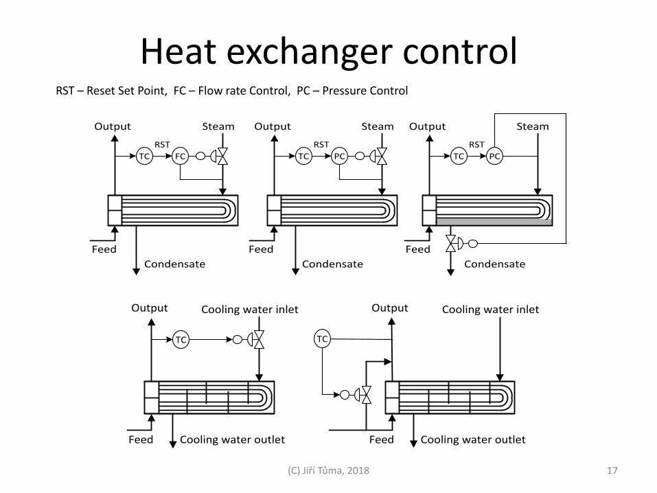
Heat exchanger control


RST – Reset Set Point, FC – Flow rate Control, PC – Pressure Control

Condensate

Steam

Feed

FC

Output

RST

TC

Condensate

Steam

Feed

PC

Output

TC

Condensate

Steam

PC

Output

TC

Feed

RSTRST

Cooling water outlet

Cooling water inlet

Feed

Output

TC

Cooling water outlet

Cooling water inlet

Feed

Output

TC

Standard ISO 3511-1 vs. 3511-2


FI 3

Impulse

pipe instruments

3 valves display

ISO 3511-1

Flow rate, Indicating Flow rate, Indication - details

ISO 3511-2

Piping system

Orifice

Flow rate measurement with display at process control console

Standard ISO 3511-2


Diaphragm actuator Rotary motor actuator

Solenoid actuator Diaphragm actuator, pressure-balanced

Solenoid actuator with reset

Piston actuator Orifice plate Venturi tube

Nozzle Variable area meter Turbine meter Volume meter

M

H

FQ

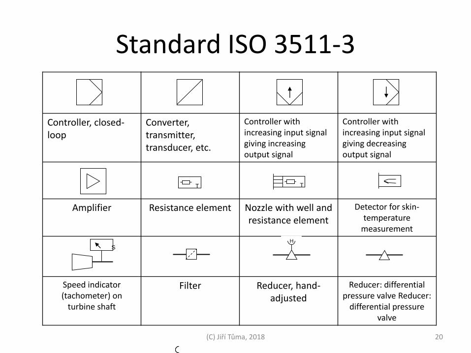
Standard ISO 3511-3


Controller, closed-loop

Converter, transmitter, transducer, etc.

Controller with increasing input signal giving increasing output signal

Controller with increasing input signal giving decreasing output signal

Amplifier Resistance element Nozzle with well and resistance element

Detector for skin-temperature

measurement

Speed indicator (tachometer) on

turbine shaft

Filter Reducer, hand-adjusted

Reducer: differential pressure valve Reducer:

differential pressure valve

H

S

T T

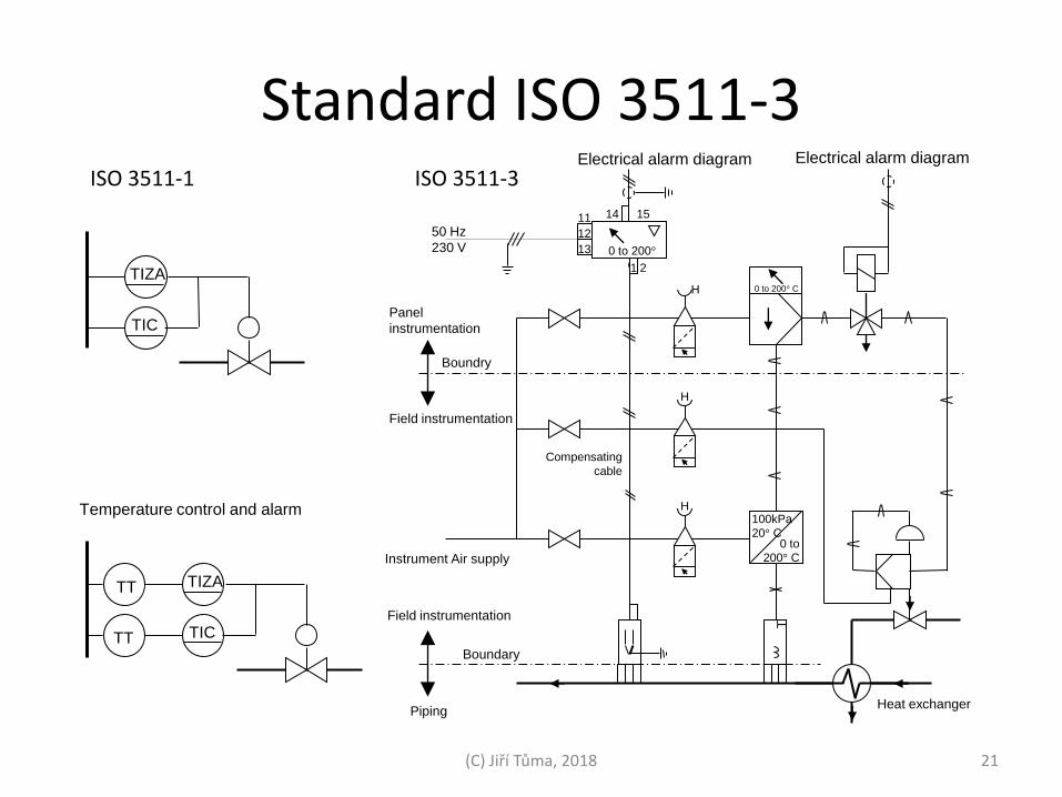
Standard ISO 3511-3


H

H

H

0 to 200° C

100kPa

20° C 0 to

200° C

T

0 to 200°

C

Electrical alarm diagram

Heat exchanger

Boundary

Boundry

Piping

Field instrumentation

Field instrumentation

Panel

instrumentation

Instrument Air supply

50 Hz

230 V

Compensating

cable

1 2

14 15 11

12

13

Electrical alarm diagram

TIZA

TIC

TIZA

TIC

TT

TT

Temperature control and alarm

ISO 3511-1 ISO 3511-3

FESTO Company


PI flow diagram for filling level control (open and closed loop control and process protection)

ISO Standards


ISO 3511-1:1977 Process measurement control functions and instrumentation -- Symbolic representation -- Part 1: Basic requirements

ISO 3511-2:1984 Process measurement control functions and instrumentation -- Symbolic representation -- Part 2: Extension of basic requirements

SO 3511-3:1984 Process measurement control functions and instrumentation -- Symbolic representation -- Part 3: Detailed symbols for instrument interconnection diagrams

ISO 3511-4:1985 Industrial process measurement control functions and instrumentation -- Symbolic representation -- Part 4: Basic symbols for process computer, interface, and shared display/control functions

This part of ISO 3511 specifies instrument symbols for use on interconnection diagrams used for the design, installation, and maintenance of process measurement and control systems. These detailed symbols are not normally intended for drawings that use the functional symbols given in ISO 3511/1 and ISO 3511/2. However, the symbols specified in this part of ISO 3511 show, by detailing the components, the external connections between units of equipment. Information on the internal connections in units is not normally included, but references to the appropriate circuit or wiring diagrams may be provided.

Servomechanism or position control

Position feedback

Velocity feedback Motor

RP RV Controller output

RP … position controller RV … velocity controller

Ball screw

Ball screw

Linear encoder

Servomechanism for positioning of the table of a machine tool


Reference velocity

Reference position

//upload.wikimedia.org/wikipedia/commons/8/81/BallScrews-with-detail-insets.jpg

Digital control systems

Controller Amplifier Actuator Plant

S1

S2

Disturbance

w

Process variable e u

v

y DAC

ADC

ADC

Analog Digital

SP CO PV

ADC analog to digital convertor

DAC digital to analog convertor


Digital control systems

PrinterVideo Display

Unit

InterfacingHardware

Analog Control Subsytem

Alarming Functions

Supervisory Control Computer

Data Storage Acquisition

System

...


Controllers

o mechanical o hydraulic o pneumatic o electronic

PID controllers

Parallel connection

e u

1

I

D

+

+

+ P

The PID controller three-term control: the proportional, the integral and derivative values, denoted P, I, and D,

P I D

The controller output u(t) is a weighted sum of P, I and D:

kP … proportional gain TI … integrating time constant TD … derivative time constant

ID TT 4


Proportional action Integral action Derivative action

u(t) … controller output, control variable, manipulated variable

e(t) … error

Parameters:

t

teTe

Ttektu D

I

Pd

dd

1

29

Properties of transfer functions The transfer function of the linear time-invariant system is a ratio of two polynomials of the complex variable s is as follows

rdenominato

numerator

...

...

011

1

011

1

sN

sM

asasas

bsbsbsb

sU

sY

tuL

tyLsG

nn

n

mm

mm

nnn

nn

mmm

mm

pspspsasasassN

zszszsbbsbsbsbsM

211

1

1

2101

1

10

...

...

If the roots of the polynomial numerator are designated by and the polynomial denominator are designated by then

mzzz ,,, 21

nppp ,,, 21

mzzz ,,, 21

nppp ,,, 21 … are called zeros of the transfer function … are called poles of the transfer function

If the parameters of the transfer function are real then the poles and zeros are complex conjugate

Complex plane

Re

Im

1z1p

2p

3p 2z


a factored form in which the polynomial is written as a product of irreducible polynomials and a constant

Domains


Time domain

s-plane domain

Complex plane

Re

Im

1z1p

2p

3p 2z

Imaginary axis

Real axis

t 0

TtT

kty exp

The Laplace transform converts integral and differential equations into algebraic equations

0

dexp tsttftfLsF

Presentation of functions in the time domain means to show them as the function of time

Example

The time functions can be transformed into the s-plane domain with the use of Laplace transform. It concerns only the deterministic functions and the mathematical operations. The time functions are converted into the functions of the complex variable s.

A tool for demonstration positions of zeros and poles of the complex functions is a complex plane.

31

Elementary transfer functions

Static

0ksU

sYsG

k0 is a gain, TI is an integral time constant and TD is a derivative time constant.

Integral

ITssU

sYsG

1

Derivative

DTssU

sYsG

The first order system

10

0

Ts

k

sU

sYsG

The first order system

11 21

0

TsTs

k

sU

sYsG

12 0

22

0

0

sTsT

k

sU

sYsG

Linear transfer functions

(without overshot) (with overshot)

tukty 0

t

I

uT

ty0

d1

t

tuTty D

d

d

tuktytyT 00 tuktytyTTtyTT 02121 tuktytyTtyT 00

2

0 2

Time delay

dTtuty

dsTe

sU

sYsG


32

Step and impulse responses

input signal x(t) Linear system

output signal y(t)

Consider a linear time-invariant system with an input x(t) and an output y(t) as follows

Let the input signal be a Dirac delta function x(t) = δ(t), X(s) = 1, then

sGsXsGsY - an impulse response of a linear system

Let the input signal be a step function x(t) = 1, X(s) = 1 / s, then

ssGsXsGsY - a step response of a linear system

(forcing function) (response of the system)

thtgsGL 1

t

gthssGL0

1 d

The impulse response is defined for x(t) = δ(t), X(s) = 1

The step response is defined for x(t) = 1, t >= 0 and x(t) = 0, t < 0, X(s) = 1 / s

t 0

1

ttx

t 0

1

ttx

1

(Heaviside) step function

Dirac delta function


PID controllers – cont’

t

teTe

Ttektu D

I

Pd

dd

1

The PID controller three-term control:

Heuristically, these values can be interpreted in terms of time: P depends on the present error, I on the accumulation of past errors, and D is a prediction of future errors, based on current rate of change.

t

teTteT

t

teteTte DDD

d

d

The derivative term

The prediction of future errors Approximation using a Taylor series

sT

sTk

sE

sUsG D

I

PPID

11

The Laplace transform of the transfer function of the PID controller:


PID controllers – interacting parameters Parallel connection

e u

P

I

D

+

+

+

Transfer function of parallel connection

sT

sTksT

sTksG D

I

PD

I

PPID

11

1 *

*

e u P

D I

+ +

+ +

Serial connection

sT

sTksT

sTk

sE

sUsG D

I

PD

I

PPID

111

11 *

*

*

where PDDIPI kTTTkT **,

******** ,,1 DIDIDDIIIDP TTTTTTTTTTk

where

Transfer function of serial connection

e u kP

+

+

sTI1

1

Transfer function of a PI controller

sT

k

sT

ksGI

P

I

PPI

11

1

11

1Positive feedback

PI controller


Proportional mode


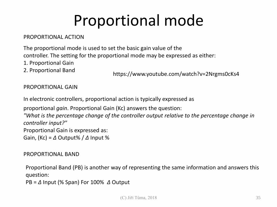
Proportional Band (PB) is another way of representing the same information and answers this question: PB = Δ Input (% Span) For 100% Δ Output

PROPORTIONAL ACTION

The proportional mode is used to set the basic gain value of the controller. The setting for the proportional mode may be expressed as either: 1. Proportional Gain 2. Proportional Band

PROPORTIONAL GAIN

In electronic controllers, proportional action is typically expressed as

proportional gain. Proportional Gain (Kc) answers the question: "What is the percentage change of the controller output relative to the percentage change in controller input?" Proportional Gain is expressed as: Gain, (Kc) = Δ Output% / Δ Input %

PROPORTIONAL BAND

https://www.youtube.com/watch?v=2Nrgms0cKs4

Step response of I and D terms of PID

Step function

t

0

1

e

t

0

1

e

t

0

1

e Step function Step function Step function

System t th

Step response

Dynamic system

t

0

1

(Heaviside) step function t

sTsE

sUsG

I

I

1

sTsE

sUsG DD

0

0

,1

TT

sT

sT

sE

sUsG

D

DPD

t

0

u

t

0

u

t

0

u Dirac function

Integrator output Ideal differentiator output Differentiator output

T0


Responses of PID, PD and PI

t

0

1

t

0

e

u

t

0

1

e

t

0

1

e Step function Step function Step function

sT

sTksG D

I

PPID

11

PID output

Ideal PID

Pkt

u PI output

Pk

sTksG

I

PPI

11

t

0

u PD output

Ideal PD

Pk

sTksG DPPD 1

dB

ω 0

ω

-π/2

0 phase

dB

ω 0

ω

π/2 phase

dB

ω 0

ω

-π/2

0

phase

0

+π/2

IT

1

DT

1

DT

1IT

1

37

0


Filtered derivative PD

Filtered derivative PID

Ideal PID Ideal PD

10 102 103 10 102 103

10 102 103

Phase lead and lag compensator

ps

zs

sE

sUsG lagLead

/

Transfer function of a compensator is as follows

Phase Lead compensator Phase Lag compensator

dB ω

0

ω

-π/2

0 phase

dB ω

0

ω

π/2 phase

0

where z is the zero and p is the pole of the transfer function. The pole and zero are both typically negative. In a lead compensator, the pole is left of the zero in the complex plane |p| > |z| , while in a lag compensator |z| > |p|

U1 U0

U0 R1

R0

C0 U1 U0

U0

R0 C1

R1

1000

00

1

0

1

1

RCRCs

RsC

sU

sU


10 102 103 10 102 103

Phase lead–lag compensator

21

21

psps

zszs

sE

sUsG lagLead

Transfer function of a compensator is as follows

Phase lead-lag compensator

dB ω

0

ω

π/2 phase

0

where z1 and z2 are the zeros and p1 and p2 are the poles of the transfer function. Typically |p 1| > |z 1|

> |z2| > |p2|

U1 U0

U0 R1

C1 R0

C0

-π/2

101100

1100

11100

00

1

0

11

11

11

1

RsCRsCRsC

RsCRsC

RsCRsCR

sCR

sU

sU


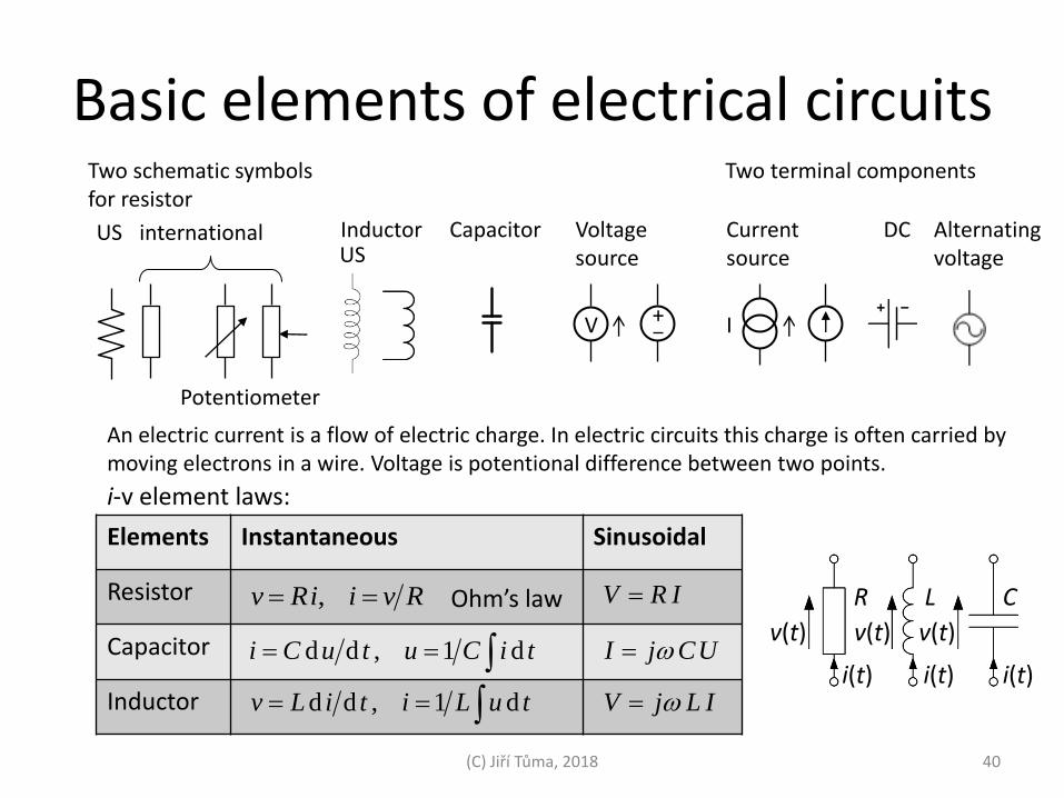
Basic elements of electrical circuits


Two schematic symbols for resistor

Inductor Capacitor

Elements Instantaneous Sinusoidal

Resistor

Capacitor

Inductor

RviiRv ,

tiCutuCi d1,dd

tuLitiLv d1,dd

IRV

UCjI

ILjV

Potentiometer

US international Voltage source

Current source

V I

DC Alternating voltage

i(t) i(t) i(t)

v(t) v(t) v(t)

R L C

US

An electric current is a flow of electric charge. In electric circuits this charge is often carried by moving electrons in a wire. Voltage is potentional difference between two points.

+

i-v element laws:

Two terminal components

Ohm’s law

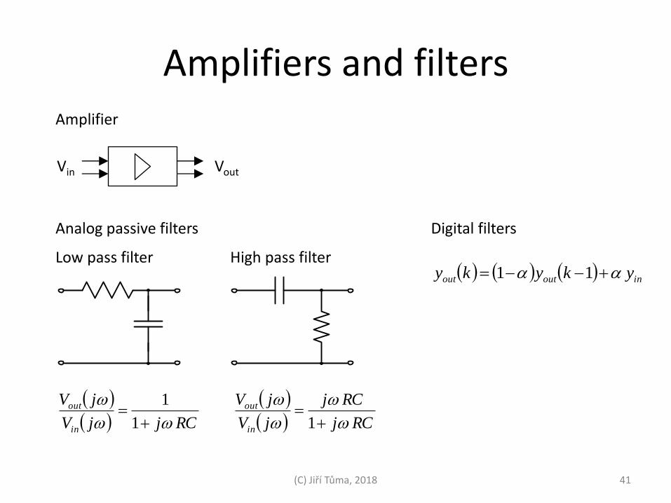
Amplifiers and filters


RCjjV

jV

in

out

1

1

Amplifier

Vin Vout

Low pass filter High pass filter

RCj

RCj

jV

jV

in

out

1

Analog passive filters Digital filters

inoutout ykyky 11

Operational amplifiers


ΔV V0 = A ΔV

Operational amplifier (“opamp”)

high gain … A (105)

An operational amplifier (op-amp) is a DC-coupled high-gain electronic voltage amplifier with a differential input and, usually, a single-ended output.

V1

V0

Voltage follower (Unity Buffer Amplifier)

11

1

10

10

010

AVV

AAVV

VVAV

ΔV V0 = A ΔV

R1

R0

V1

I

1

0

1

0

0

0

1

1

R

R

V

V

R

V

R

VI

Inverting amplifier

10 VV

AFor

- High input impedance - Low output impedance

Impedance transformer

Virtual ground

http://en.wikipedia.org/wiki/File:Ua741_opamp.jpg

//upload.wikimedia.org/wikipedia/commons/7/72/Generic_741_pinout_top.png

Electronic PID controllers

ΔV V0 = A ΔV

R1

C0

V1

I Inverting integrator

t

VCR

Vt

VC

R

VI

0

1

01

000

1

1 1 d

d

d


ΔV V0 = A ΔV

C1

R0

V1

I

Ideal inverting differentiator

t

VCRV

R

V

t

VCI

d

d

d

d 1100

0

011

V0

C1

R0

V1 Filtr

Inverting differentiator

Electronic PID controllers – cont’

DIP

DIPDIP

VVVV

R

V

R

V

R

V

R

VIIII

0

0

0

R1P

R0P

V1

R1I

C0I

C1D

R0D

R

R0

I

R

R

V0

IP

ID II

VP

VI

vD

Addition of three signals


PID controller with interaction

V1 V0

Phase lead-lag controller

V1 V0

V0

Voltage follower

Passive PID controller

Switched-Capacitor Resistor Equivalent


Switched capacitors are replacing resistors. They also allow continuous variation of the resistance by changing the switching frequency. This circuit is composed of a capacitor and analog switches and can be realized in MOS technology (which is based on MOS transistors and capacitors with capacitance in range of farads) with low costs. The switched capacitors is used for tunable filters and tunable and for amplifiers, voltage-to-frequency converters, programmable capacitor arrays, oscillators, amplifiers.

Since the clock signal for the second MOSFET is inverted, one transistor is turned on (its resistance is around 1-10kΩ), and the second is turned off (its resistance is of the order of 1012 kΩ). Therefore MOSFETs can be considered as switches.

C

Clock1 Clock2 = Clock1

Vin Vout

Change of the capacitor charge

If the switching occurs N times per a second, then the amount of charge in the capacitor per the time interval of the Δt length, which is an electric current, is

The resistor equivalent of the circuit can be calculated as

where is a clock frequency. tNfclock

Switched-Capacitor Resistor Equivalent


C

Clock1= 1 Clock2 = Clock1 = 0

Vin Vout

C

Clock1= 0 Clock2 = Clock1 = 1

Vin Vout

Parasitic-Sensitive integrator


The resistance increases with decreasing capacitance or with decreasing switching frequency

Cs

Cfb

Vout Vin

Clock

Resistor

Inverted Clock

tNfclock

Often switched capacitor circuits are used to provide accurate voltage gain and integration by switching a sampled capacitor onto an op-amp with a capacitor Cfb in feedback. One of the earliest of these circuits is the parasitic-Sensitive integrator developed by the Czech engineer Bedrich Hosticka. The time constant of the integrator is adjustable through changes frequency of the clock signal

Req

Switched Capacitor Circuits, Swarthmore College course notes, accessed 2009-05-02.

Parasitic from fringing capacitors and bottom-plate to substrate

C1

Cp1 Cp2

12 %20 CCp

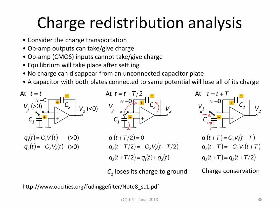
Charge redistribution analysis


http://www.oocities.org/fudinggefilter/Note8_sc1.pdf

• Consider the charge transportation • Op-amp outputs can take/give charge • Op-amp (CMOS) inputs cannot take/give charge • Equilibrium will take place after settling • No charge can disappear from an unconnected capacitor plate • A capacitor with both plates connected to same potential will lose all of its charge

C1

C2 V2 (<0) V1

tVCtq

tVCtq

222

111

C1

C2 V2 V1

2Ttt

22

02

222

1

TtVCTtq

Ttq

tt At At

tqtqTtq 212 2

C1

C2 V2 V1

Ttt

TtVCTtq

TtVCTtq

222

111

At

222 TtqTtq

C1 loses its charge to ground Charge conservation

(>0)

(>0)

(>0) 0 0 0

Transfer Function


http://www.oocities.org/fudinggefilter/Note8_sc1.pdf

Inverting Discrete-time Integrator

tqtqTtqTtq 2122 2

tVCtVCTtVC 221122

zVCzzVC

zVCzVCzzVC

1122

221122

1

1

1

2

1

2

1

1

2

11

1

z

z

C

C

zC

C

zV

zVzH

Z-transform

Transfer function

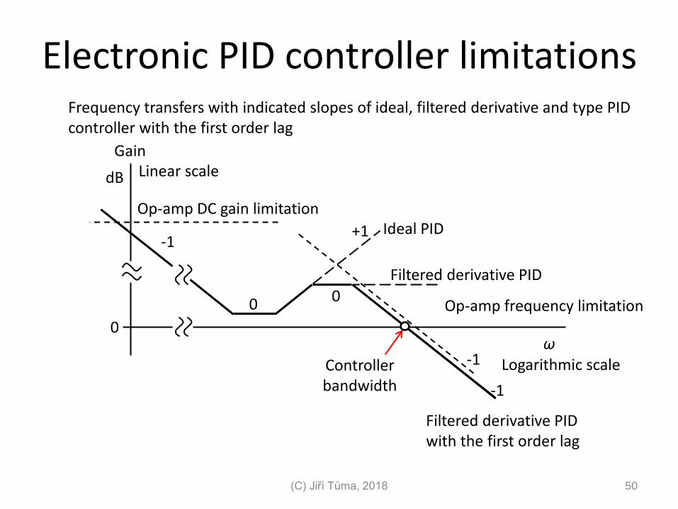
Electronic PID controller limitations


ω 0

dB

Op-amp DC gain limitation

Ideal PID

Filtered derivative PID

Op-amp frequency limitation

Controller bandwidth

Gain

Frequency transfers with indicated slopes of ideal, filtered derivative and type PID controller with the first order lag

-1

-1

-1

0 0

+1

Filtered derivative PID with the first order lag

Logarithmic scale

Linear scale

Programmable logic controllers - PLC


Programable Logic Controller

+24V

relays valves lamps, lights

Input binary signals

PLC acts as an electric switchboard which is a device that directs electricity from one source to another.

Output binary signals

E

Logic control

Linear control

PID control – 1 or 2 closed loops including frequency converter

PID controllers for PLC

P

I

D

+ P Slew Time Clamp Dead Band

CO Polarisation

Bias

SP

PV

-

P

I

D

+ P Slew Time Clamp Dead Band

CO Polarisation

Bias

SP

PV

-

Block diagram of PIDIND

Block diagram of PIDISA

CO … Controller Output, control variable, manipulated variable PV … Process Variable, controlled variable, measured variable SP … Set Point, desired value, reference signal, command Bias … a value added to the controller output.

Bias can be used as the offset for Feed-forward Control


Digital PID controllers

Biast

ektekekCO DIP d

dd

t

ektekekCO DIP

d

ddddd

21211 kekekeT

kkTekkekekkCOkCO D

IP

21211 kPVkPVkPVT

kkTekkekekkCOkCO D

IP

21211 kPVkPVkPVT

kkTekkPVkPVkkCOkCO D

IP

CO … Controller Output PV … Process Variable SP … Set Point e = SP – PV (error) measured error Bias … a value added to the controller output

Type A

Type B

Type C

PID controller

After differentiation

Parameters kP … proportional gain kI … integral gain kD … derivative gain T … sample period k … discrete time

T

keke

t

e

kekee

kCOkCOCO

1

d

d

1d

1d


PID controllers as a part of PLC Features • Bumpless transition between manual and automatic

mode • Bias can be used as the offset for Feed-forward Control

When PID is active, declared Sample Period is compared with elapsed time from the previous algorithm execution. If it is greater then successive iteration is carried out. If calculated CV is outside the range Lower Output Clamp − Upper Output Clamp, or it changes faster than declared Minimum Slew Time then CV is limited to appropriate value and value in buffer memory in integral term is adjusted (anti-reset windup).

Calculated CV is also stored in Manual Command register as well as in Internal CV register, assuming PID is in AUTO mode. If the block is in manual mode (Boolean 1 on the input MAN), then CV is equal to the value in Manual Command register, which can be incremented (1 on UP) or decremented (1 on DN). In manual mode the output value can be written manually from a programmer as well.


Distributed control systems

Process Transmitters and Actuators

Data Highway(Shared Communication Facilities)

......

DataStorage Unit

HostComputer

System Consoles

PLC

4-20 mA

LocalConsole

LocalControl

Unit

4-20 mA

LocalControl

Unit

LocalConsole


Industrial buses

Plant Optimization

.................

Smart Sensors

Smart ControlValves and Controllers

LocalArea

Network

Smart Sensors

Smart ControlValves and Controllers

LocalArea

Network

H1 Fieldbus Network H1 Fieldbus Network

H1 Fieldbus H1 Fieldbus

Data Storage

PLCs

High Speed Ethernet


Hydraulic and pneumatic controllers

Flapper – nozzle principle

Δx

p0

p

nozzle

flapper

p0

p

Δx

cca 0,02 mm

Air supply

output pressure

gap

p

pressure setting

p0 p

ress

ure

ve

ssel

spring bellows

pneumatic actuator

Nozzle-flapper

Schematic arrangement of the flapper – nozzle system

fulcrum

An equivalent of a simple operational amplifier (“opamp”) circuits with analogous pneumatic mechanisms

nozzle

Air pressure p

orifice

Pressure vs. width of gap


Approximate linear range

http://en.wikipedia.org/wiki/File:Metal_bellows.jpg

//upload.wikimedia.org/wikipedia/commons/8/81/Pressure_Vessel.jpg

Hydraulic valves

p0 p1

p2

p0

p1 p2 Δx

Δp = p1 - p2

Δx Jet Pipe

Double-nozzle Flapper

Pressure difference

Δx

Receiver block

Fluid Supply

Chamber A

Leakage

path

Supply pressure

Δx > 0

Valve

spindle

Δx = 0

Chamber B

Lands Under

Lapped

Valve

Over

Lapped

Valve

Δx – valve position

Δx

Zero

Lapped

Valve

Control flow

Under Lapped Valve Zero Lapped Valve

Over Lapped Valve

A servo consists of a spool (two lands connected by a rod) and an outer sleeve (sometimes called a bushing) with flow ports drilled in the sleeve. The position of the spool determines the flow areas and hence controls the amount of flow through the valve. Cut-away drawing …

Servo lapping

Orifice

59

Spool valves

http://www.youtube.com/watch?v=U5iXiRxBcJo&list=PL8245A490BE8A8C9D


Valve types

60

https://www.qualityhydraulics.com/blog/what-proportional-valve/


Directional Control Valves Traditional hydraulic equipment designs used directional control valves almost exclusively. These valves are used to control flow direction. It can be referred to as either “switching” or “bang-bang” valves. Proportional Valves For solving the more complex circuits, proportional valves have been developed. These valves allow infinite positioning of spools, thus providing infinitely adjustable flow volumes. Either stroke-controlled or force-controlled solenoids are used to achieve the infinite positioning of spools. The proportional valve is any continuously variable, electrically modulated, directional control valve with more than 3% center overlap.

Servo Valves The third type of hydraulic directional control technology is the servo valve. The servo valves were first used in the 1940s. These valves operate with very high accuracy, very high repeatability, very low hysteresis, and very high frequency response. The servo valves are used in conjunction with more sophisticated electronics and closed loop systems.

Proportional valves

61

http://www.iranfluidpower.com/pdf/All%20hydraulics/Proportional%20Valves.pdf


Armature

x = 0

Coil

Coil

Pole piece

Force

x = xmax

Force Force

Working Stroke Working Stroke

Conventional solenoid Proportional solenoid

Current

Current

Spring Balance Positiom Feedback

Fa Fa Fk

i i

V ka

Vin

Vf

+V -V

Feedback Voltage

x x

F F

F

Control current Control Voltage

Force Balance Position

Sensor

Spring

Flux Paths

2

2

00

2n

lx

ii

f

AF

e

M

Wire turns

Force

Symbols in a hydraulic schematic 1


Continuous line - for flow line Dashed line - for pilot, drain

Envelope - for dashes around two or morecomponent symbols

Large Circle - pump, motor

Small Circle - measuring devices

Semi-circle - rotary actuator

Flow restriction (affected by viscosity)

Spring

Lines

Circles Square

One square - pressure control function

Two or three adjacent squares - directional control

Triangle Solid - Direction of Hydraulic Fluid Flow

Open - Direction of Pneumatic flow

Diamond

Diamond - Fluid conditioner (filter, separator, lubricator, heat exchanger)

Miscellaneous Symbols

Pump and Compressor Symbols

Unidirectional

Bidirectional

Compressor Symbol

Fixed Displacement Hydraulic Pump Symbol

Bidirectional

Semi-circle - rotary actuator

Variable Displacement Hydraulic Pump Symbols

Adjustable output flow – Needle Valve

Orifice (un-affected by viskosity)



Cylinders Hydraulic Motor Symbols

Unidirectional Fixed Displacement Hydraulic Pump Symbol Bidirectional

Unidirectional Variable Displacement Hydraulic Pump Symbol

Bidirectional

Pneumatic Motor Symbols

Unidirectional

Bidirectional

Rotary Actuator Symbols

Hydraulic

Pneumatic

Single acting (returned by external force)

Double acting single rod end

Double acting double rod end

Single acting (returned by spring force)

Cylinders with Cushions Symbols

Single fixed cushion

Double fixed cushion


2 position – 2 way valve



3 position – 4 way valve Closed Center Valve

Valve capable infinite positioning (indicated by horizontal lines drawn parallel to the envelope

Valves Check valve symbol-free flow one direction

On-Off manually shunt off

Manual Valve Control

Spring

Manual general symbol

Hydraulic actuated pilot

Pressure relief valve

Reservoir open to atmosphere


Open Center Valve

Push Button

Lever

Foot pedal

Mechanical Valve Control

Roller

Pilot Operation (uses pressure to actuate valve)

Solenoid (the one side's winding shown)

Pneumatic actuated pilot

Electrical/Solenoid Valve Control

P

T

Normally closed valve

Pilot port

Pressurized Reservoir

Symbols in a hydraulic schematic 4 Pilot operated two-stage valve (uses a second lesser force to actuate the pilot actuation of the valve)



P

T

Normally closed valve

Pilot port

Pneumatic: Solenoid first stage

Hydraulic: Solenoid first stage

Pneumatic: Air pilot second stage

Hydraulic: Air pilot second stage

Single-stage direct operation unit which accepts an analog signal and provides a similar analog fluid power output

Electro-Hydraulic Servo Valve

Two-stage with mechanical feedback indirect pilot operation unit which accepts an analog signal and provides a similar analog fluid power output

Electro-Hydraulic Servo Valve

To isolate one part of a system from an alternate part of circuit.

Symbols in a hydraulic schematic 5 Filter, Water Trap, Lubricator, and Miscellaneous Apparatus Symbols


Filter or Strainer

Filter or Strainer

With manual drain

Water Trap

With automatic drained

With manual drain

Filter with Water Trap

With automatic drained

Refrigerant, or chemical removal of water from compressed air line

Air Dryer

Oil vapor is injected into air line

Lubricator

Conditioning Unit (FRL, Pressure Regulator)

Compound symbol of filter, regulator, lubricator unit (FRL symbol)

Simplified Symbol

Servovalves

http://www.daerospace.com/HydraulicSystems/

Flapper Nozzle Servovalve Jet Pipe Servovalve


Electro-hydraulic servo valves

A B

T P

A B

T P P P

p1 p2

T

A B

T P P P

p1 p2

T

Proportional valve

An Electro-Hydraulic Servo Valve or EHSV is an electrically operated valve that controls how hydraulic fluids is ported to an actuator. Servo valves can provide precise control of position, velocity, pressure and force with good post movement damping characteristics

Centering spring

Fixed orifis

Pilot or control line

Hydraulic: Solenoid first stage with internal pressure

Stage 1

Stage 2

To actuators

Supply pressure

Tank

Supply pressure

Spring

Steady-state position Transient position


P P

Directional control valves

Four Way, Three Position (4/3) Valve

Directional valves are valves that direct flow in response to external commands. These valves do not provide flow or pressure regulation and functional only to direct flow (much like a switch). They usually consist of a spool inside a cylinder which is mechanically or electrically controlled.

2-Positions, 3-Positions, 4-Positions

2-way On-Off for fluid supply

3-way Single acting cylinders

4-way Double acting cylinders

5-way Pneumatic system with dual air pressure

P T

A B spring

solenoid

Valve actuator

Double acting

cylinders Single rod end

a b 1 3

2 a b

1 3

2

Normally closed

Three Way, Two position (3/2) Valve

Normally open

Single acting pneumatic cylinders with return spring

Manually actuated

M

Hydraulic accumulator

Unidirectional pump

Double acting cylinder

4/3 valve


motor

filter

Supply line

Port B Port A

Control valve


Three-way, two-position (3/2) valve, normally closed


a b

1 3

2

No oil flow to the cylinder chamber

Manually actuated

Initial position

a b

1 3

2

Oil starts to flow to the cylinder chamber

Manually actuated

After pressing the valve actuator

1 3

2

a b a b

3-way valve

Electro-pneumatic circuits

Electric circuits

Pneumatic actuator with return spring

a b

1 3

2

S

Q

Q Q

24V DC

0V 3/2 valve

Normally open button

Normally closed

Coil

contact


Sensors

Measurement systems Input

Sensor Output

Physical quantity (stimulus ): Displacement, speed, RPM, acceleration, pressure, temperature, force, flow rate, ……

Signal in observable form: Voltage, electric current, pressure, digital Signal type: Binary (true/false), (log 0/log 1), (low/high) Analog (0 to 10 V, -5V to +5V, 4 to 20 mA) Digital


A transducer is a device that converts one form of energy to another form of energy. The term transducer commonly implies sensor or detector or probe. Transducers are widely used in measuring instruments.

Principle of sensors

Sensor

Transducer 1

Stimulus

Jacob fraden: Handbook Of Modern Sensors Physics Designs And Applications


A sensor is a device that receives a stimulus and responds with an electrical signal.

Transducer 2 Direct sensor e2 e1 e3

Electric signal

e1 , e2 , e3 , and so on are various types of energy.

The term sensor should be distinguished from transducer. The latter is a converter of one type of energy into an other,whereas the former converts any type of energy into electrical. Transducers may be parts of complex sensors. This suggests that many sensors incorporate at least one direct-type sensor and a number of transducers. The direct sensors are those that employ such physical effects that make a direct energy conversion into electrical signal generation or modification. An example of a transducer is a loudspeaker which converts an electrical signal into a variable magnetic field and, subsequently, into acoustic waves. This is nothing to do with perception or sensing.

Transducers may be used as actuators in various systems. An actuator may be described as opposite to a sensor—it converts electrical signal into generally nonelectrical energy.

Performance terms - 1 Accuracy and error

Error = measured value – true value

Hysteresis error

Input: Physical quantity

Output signal

hysteresis

Non-linearity error


Output signal

Non-linearity error

Assumed relationship

Actual relationship

Insertion error due to the loading

Measurement range

Precision, repeatability and reproducibility

Measured values

True value

High precision, low accuracy

Measured values

True value

Low precision, low accuracy

Measured values

True value

High precision, high accuracy The range of variable of system is the limits between which the input can vary.


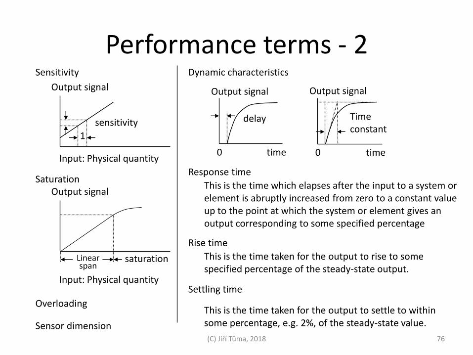
Performance terms - 2 Sensitivity


Output signal

sensitivity

1

Dynamic characteristics

Overloading

Sensor dimension

time

Output signal

delay

0 time

Output signal

Time constant

0

Response time

Rise time

Settling time

This is the time taken for the output to settle to within some percentage, e.g. 2%, of the steady-state value.

This is the time taken for the output to rise to some specified percentage of the steady-state output.

This is the time which elapses after the input to a system or element is abruptly increased from zero to a constant value up to the point at which the system or element gives an output corresponding to some specified percentage



Output signal

saturation Linear span

Saturation

Output impedance


Interface circuit Sensor Interface circuit

V Zout Zout

I

Zin

Zin

IS

VS

Sensor

Sensor has voltage output Sensor has current output

The output impedance Zout is important to know to better interface a sensor with the electronic circuit. This impedance is connected either in parallel with the input impedance Zin of the circuit (voltage connection) or in series (current connection). The output and input impedances generally should be represented in a complex form, as they may include active and reactive components. To minimize the output signal distortions, a current generating sensor should have an output impedance as high as possible and the circuit’s input impedance should be low. For the voltage connection, a sensor is preferable with lower Zout and the circuit should have Zin as high as practical.

Principles of sensors


Measuring chain in detail

Physical quantity → low voltage → electrical signal (voltage or current)

Physical quantity → electrical resistance → electrical signal

Physical quantity → force → electric current in the compensation electromagnet → electrical signal

Physical quantity → displacement → inductance → electrical signal

Strain → electrical resistence → the electrical signal

Velocity → V = B v l → electrical signal

Velocity → pulse frequency → electrical signal

Velocity → pulse frequency → length of time interval → the electrical signal

Velocity → difference frequency → electrical signal

Velocity → frequency schift (Doppler effect: sound, ultrasound or light) → electrical signal

The gas content with asymmetrical molecule (CO, CO2) → electrical resistance → electrical signal

The oxygen content in the gas → electrical resistance → electrical signal

kRRll ,

Wheatstone bridge

R1

R2

Rx

R3 Output voltage

Power supply 32

1

R

R

R

R xR1

R2

R4

R3 Output voltage

Power supply

A Wheatstone bridge is an electrical circuit used to measure an unknown electrical resistance by balancing two legs of a bridge circuit, one leg of which includes the unknown component. Its operation is similar to the original potentiometer.

Input: Detector Output: Physical quantity Wheatstone

bridge

Sensor

Voltage signal

strain gauge. resistance thermometer

R is the unknown resistance to be measured

R

The point of balance is the ratio

2

13

R

RRRx

VS

0V

V0

0V

S

x

xG V

RR

R

RR

RV

21

2

3

VG VG

0aI

0bI

0aV

0bV

Output voltage of the Wheastone bridge

VS 4-wire circuit

resistance

Line resistance


Sensors for Displacement


Linear variable differential transformer (LVDT)

Proximity sensors

Linear optical sensors

Confocal chromatic sensors

Strain gauges

Extensometers

Encoders

Magnetostrictive sensors

Draw-wire sensors

Displacement sensors

Δx

Δx

Δx

Δx

Δx

Δx

Δx ΔL

Δx ΔL1 ΔL2

Δx

ΔL Δx

ΔV

V0 Δx

V1

V1 V2

V0 V2

A) B) E)

C) D) F)

Capacitive sensing

where C is the capacitance, ε0 is the permittivity of free space constant, K is the dielectric constant of the material in the gap, A is the area of the plates, and d is the distance between the plates.

d

KAC 0

Inductive sensors

The inductance of the loop changes according to the material inside it and since metals are much more effective inductors than other materials the presence of metal increases the current flowing through the loop.

A, C) powered by AC

Δx ΔL

ΔL1 ΔL2

Δx

V = V1 - V2

Δx B, D)

Potentiometer

R1 Output voltage

Power supply R2

VL +VS

0V load

SL Vx

xV

Rx

xR

Rx

xR

12

1


wiper (slider)

(sliding contact)

Linear variable differential transformer


(LVDT)

V2

V1

Δx

Vout = V1 - V2

core

Vin LVDT’S AC Output Magnitude

Null Position

50% 100% 0%

AC Output Magnitude of Conventional LVDT Versus Core Displacement

Out Of Phase In Phase

Small-displacement sensors

Z

d

Oscilator Z d

Z0

u0 u

Demod

synchronisation

X

Y

Eddy-current sensor Capacitive sensor

Journal of a sleeve bearing

i ~ d

i2 H2

H1

Softmagnetic ferrite

Steel

Eddy current

magnetic field lines magnetic intensity

Proximity probe


Linear optical sensors


Light source lens

LED

Driver circuit

Amplifier circuit

Optical position detector element

Receiver lens

Design of a one-dimensional position-sensitive detector (PSD)

A PSD operates on the principle of photo effect.

The position of an object is determined by applying the principle of a triangular measurement.

Confocal chromatic sensors


The axial position of the focal point of an uncorrected lens depends on the color (wavelength) of the light to be focused. In the visible spectral region, the focal distance for blue light is minimal while it is maximal for red light. The focal points of other colors are located in between according to the row: red, orange, yellow, green, blue, violet. Depending on the distance of the target from the focusing lens, light of just a very small wavelength region Ȝ1 is focused on the target’s surface (Fig. 1). All other spectral components of the light source are illuminating a much wider area of the surface.

Halogen lamp

Fiber optics

Fiber coupler

Optical probe

Surface Measuring range

The focusing lens is also used to receive the backscattered light from the target’s surface and to focus it into an optical fiber. Due to that confocal arrangement, light having the wavelength λ1 is focused to the front of the fiber and enters it without clipping. All other spectral components are spread on a much bigger area. As a consequence, the light fed through the fiber to a spectrometer is almost monochromatic, it´s wavelength λ1 being a chromatic code about the axial position of the backscattering surface of the target.

http://armstrongoptical.co.uk/wp-content/uploads/2013/08/Chromatic-Confocal-Measurement-principles.pdf

Magnetostrictive sensors


http://www.mdpi.com/1424-8220/11/5/5508/htm

Linear position sensors based on magnetostrictive effect are widely used for position measurement. In accordance with the Wiedemann effect and the Villari effect, the magnetostrictive linear position sensor (MLPS) uses a ferromagnetic material waveguide to perform accurate position measurements.

Magnetostriction


http://www.instrumentation.co.za/article.aspx?pklarticleid=5195

Alignment of magnetic domains to the applied magnetic field H

The amount of magnetostriction in base elements and simple alloys is small, on the order of 1 µε

Wiedemann effect


Sensorland.com

Current

Current Waveguide twist

Ferromagnetic material

Position magnet (permanent)

An important characteristic of a wire made of a magnetostrictive material is the Wiedemann effect. When an axial magnetic field is applied to a magnetostrictive wire, and a current is passed through the wire, a twisting occurs at the location of the axial magnetic field. The twisting is caused by interaction of the axial magnetic field, usually from a permanent magnet, with the magnetic field along the magnetostrictive wire, which is present due to the current in the wire.

Magnetostrictive Linear-Position Sensors


https://www.controldesign.com/assets/wp_downloads/pdf/mts_sensors.pdf

Magnetostrictive Linear-Position sensor with sensing rod and position magnet.

A magnetostrictive position sensor measures the distance between a position magnet and the head end of the sensing rod. The position magnet does not touch the sensing rod, and therefore there are no parts to wear out.

Magnetostrictive sensors - principle



Mechanical strain pulse

Magnet field position magnet

Magnetostrictive sensing element (waveguide)

Magnet field of current probe

Movable position magnet

Strain (torsion) pulse convertor

Current interrogating pulse

In the transducer a strain pulse is induced in a magnetostrictive waveguide by the interaction of two magnetic fields. One field comes from a moving magnet, which passes along the outside of the transducer tube, and the other field is generated from a current pulse which is applied to the waveguide.

The interaction between these two magnetic fields produces a strain pulse which travels along the waveguide until the pulse is detected at the head of the transducer. The position of the moving magnet is precisely determined by measuring the elapsed time between the application of the current pulse and the arrival of the strain pulse.

The interrogation rate can be controlled from an external controller, or can be internally generated at a rate anywhere from one time per second to over 4000 times per second.

1 or 2 µs

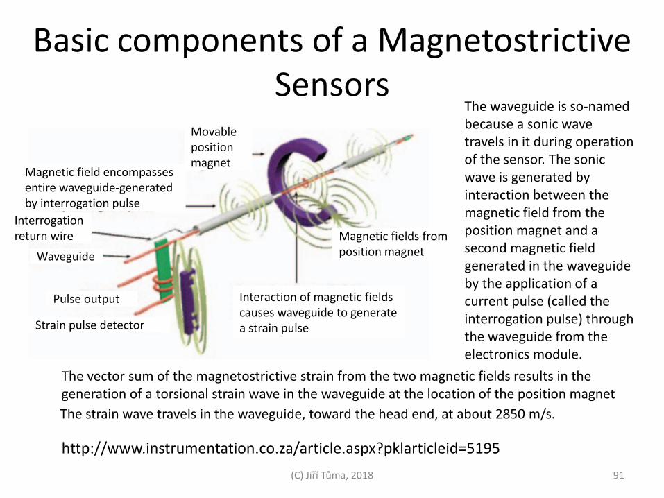
Basic components of a Magnetostrictive Sensors



Interaction of magnetic fields causes waveguide to generate a strain pulse Strain pulse detector

Pulse output

Waveguide

Magnetic fields from position magnet

Interrogation return wire

Movable position magnet

Magnetic field encompasses entire waveguide-generated by interrogation pulse

The waveguide is so-named because a sonic wave travels in it during operation of the sensor. The sonic wave is generated by interaction between the magnetic field from the position magnet and a second magnetic field generated in the waveguide by the application of a current pulse (called the interrogation pulse) through the waveguide from the electronics module.

The vector sum of the magnetostrictive strain from the two magnetic fields results in the generation of a torsional strain wave in the waveguide at the location of the position magnet

The strain wave travels in the waveguide, toward the head end, at about 2850 m/s.

Installation into space-restricted cylinders


https://www.controldesign.com/assets/wp_downloads/pdf/mts_sensors.pdf

Strain (torsion) pulse convertor

Draw-wire sensors


https://www.micro-epsilon.com/displacement-position-sensors/draw-wire-sensor/MK_Serie/#!#WPS-MK60_analog

Measuring ranges (mm):

50 | 150 | 250 | 500 | 750 | 1,000 | 1,250 | 1,500 | 2,400 | … | 3,000 | 5,000 | 7,500 Linearity ± 0.1 % F.S.O. Signal output: Potentiometer

Signal output: Incremental encoder

Draw wire sensors are compact sensors which accurately measure the position or change in position of objects. Core components of a draw wire sensor are a precision measuring wire and a sensor element (e.g. potentiometer or encoder), which convert the path change into a proportional electrical signal.

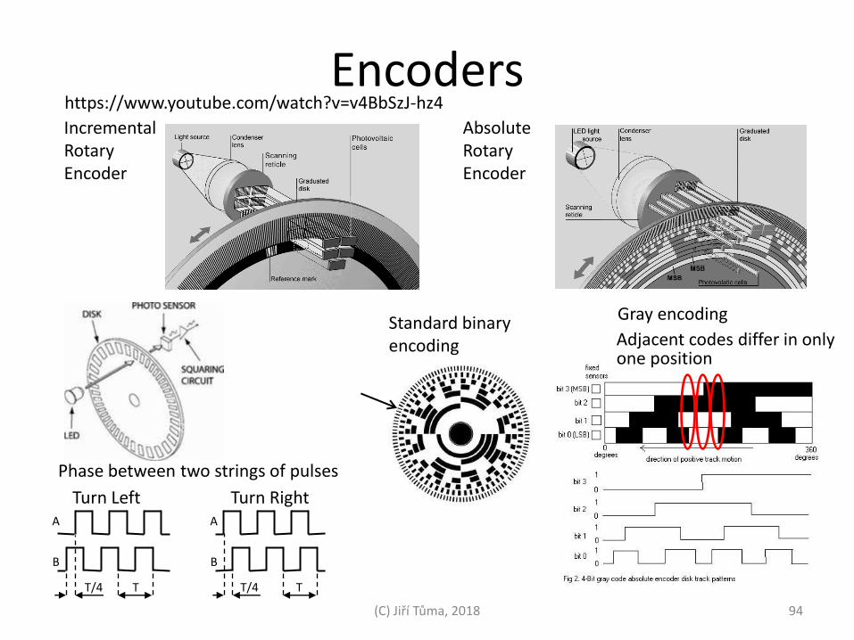
Encoders Incremental Rotary Encoder

T/4 T

A

B

Absolute Rotary Encoder

T/4 T

A

B

Turn Left Turn Right

Standard binary encoding

Gray encoding

Adjacent codes differ in only one position

Phase between two strings of pulses


https://www.youtube.com/watch?v=v4BbSzJ-hz4

http://www.google.cz/imgres?imgurl=http://www.parkermotion.com/dmxreadyv2/blogmanager/app_engine/assets/images/encoder-rot-large.jpg&imgrefurl=http://www.parkermotion.com/dmxreadyv2/blogmanager/blogmanager.asp?post=motor-feedback-options&h=600&w=598&sz=82&tbnid=gGkQ30RqthxjwM:&tbnh=87&tbnw=87&prev=/search?q=absolute+rotary+encoder&tbm=isch&tbo=u&zoom=1&q=absolute+rotary+encoder&usg=__tD_HXDG0y4w87iDCFVf3AjQvpq4=&docid=8Ayyj_oJARy4lM&hl=cs&sa=X&ei=pxV_UMyEMsjR4QT5uICgBA&ved=0CEcQ9QEwAw&dur=2881

Examples of encoders


Large Bore Hollow Shaft Encoders

Hollow Shaft Encoder Solid Shaft Encoders

Incremental Encoders Absolute Encoders

Parallel Output Format (Single Turn) with Semi Hollow Shaft

High Resolution Encoders They are available encoders with any value resolution from 1 to 65536 pulses per revolution, which in turn can be interpolated by 4 times if required for even greater resolution. A similar miracle can be provided with absolute technology too, up to as much as 20 bit resolution per turn.

Linear Encoders

Magnetic Type Optical Type

http://www.industrialencodersdirect.co.uk/wp-content/uploads/2016/06/110HA-Encoder-1-1.jpg

http://www.industrialencodersdirect.co.uk/wp-content/uploads/2016/06/51HA-Encoder-1.jpg

http://www.industrialencodersdirect.co.uk/wp-content/uploads/2016/06/40SA-Encoder-1.jpg

http://www.industrialencodersdirect.co.uk/wp-content/uploads/2016/06/58TA-Encoder-1.jpg

http://www.industrialencodersdirect.co.uk/wp-content/uploads/2016/06/MLS-3-Encoder-1.jpg

http://www.industrialencodersdirect.co.uk/wp-content/uploads/2016/06/ALS-Encoder-1.jpg

Uniformity of engine rotation


Definition of Strain


Hook’s Law StrainEStress

is the elastic modulus E

Microstrain µε = ΔL / L0 x 106

A microstrain equals the strain that produces a deformation of one part per million.

Strain ε = ΔL / L0

If ε equals to 0.1% then µε equals to 10-3 x 106 = 1000

American English use the word gage. British English is gauge. Except this, both gage and gauge mean the same.

Unstrained rod

Tensil strain Compressive strain

Metallic strain gauges are one of many devices, along with piezo resistors and devices based on interferometric techniques, that have been developed to measure microstrain. Invented by Edward E. Simmons in 1938, the metallic strain gauge consists of a fine wire or metallic foil with an electrical resistance (Ro) adhered to a flat rigid substrate. Ro typically varies from tens to thousands of ohms and the substrate is often referred to as the carrier.

Strain gauges

Metallic strain gauge Metal foil

Term

inal

s

Gauge factor

Semiconductor gauge

GFRR G

21

GRR

GFρ is resistivity

ν is Poisson’s ratio Change in strain gauge resistance

α is temperature coefficient Θ is temperature change

Material Gauge Factor Metal foil strain gauge 2-5

Thin-film metal 2 Single crystal silicon -125 to + 200 Polysilicon ±30 Thick-film resistors 100

98

Leads


120 Ω, 350 Ω, and 1,000 Ω Nominal resistance

Strain gauge type

Backing Encapsulation

Copper-coated tabs

Metallic grid pattern

Sold

er t

abs

Carrier

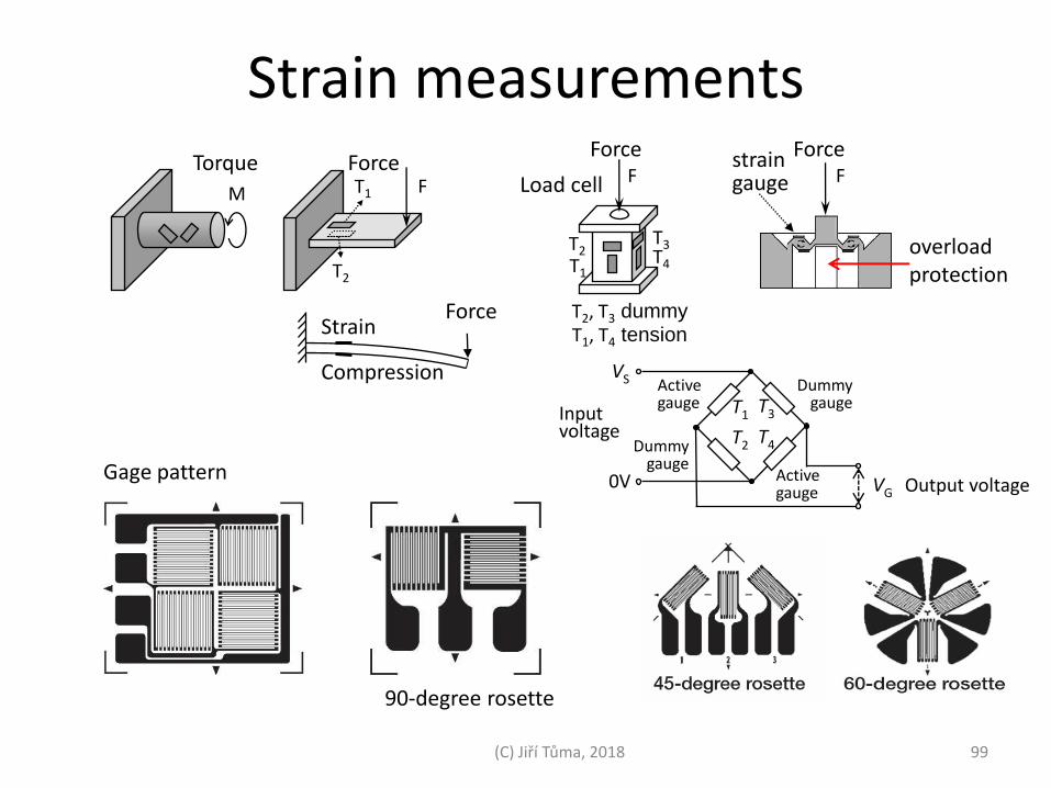
Strain measurements

Gage pattern

M F T1

T2 T1 T2 T4

T3

F

T2, T3 dummy T1, T4 tension

F Torque Force

overload protection

strain gauge

Force Force

Load cell

Strain

Compression

Force


90-degree rosette

T1

T2

T3

T4

Output voltage

Input voltage

VS

0V VG

Active gauge

Active gauge

Dummy gauge

Dummy gauge

http://www.google.cz/url?sa=i&rct=j&q=half+bridge+strain+gauge&source=images&cd=&cad=rja&docid=OaYNk7eDPWW_0M&tbnid=T8_EzHNVjSh0fM:&ved=0CAUQjRw&url=http://www.alibaba.com/product-gs/484493736/Half_Bridge_Strain_Gauge_BB.html&ei=W609UbvEG9HMswbghIDwDw&bvm=bv.43287494,d.Yms&psig=AFQjCNGJ-QK9inyfTmHbWC9TGBQOv7zC3Q&ust=1363082459278982

http://www.google.cz/url?sa=i&rct=j&q=half+bridge+strain+gauge&source=images&cd=&cad=rja&docid=OaYNk7eDPWW_0M&tbnid=erF_ouySqCJAoM:&ved=0CAUQjRw&url=http://www.alibaba.com/product-gs/484493736/Half_Bridge_Strain_Gauge_BB.html&ei=iq09UYTOO87jtQbOyIDQCQ&bvm=bv.43287494,d.Yms&psig=AFQjCNGJ-QK9inyfTmHbWC9TGBQOv7zC3Q&ust=1363082459278982

Bridge strain gauge circuits Full-bridge strain gauge circuit

Half-bridge strain gauge circuit

Quarter -bridge strain gauge circuit

100 (C) Jiří Tůma, 2018

Signal conditioning for strain gages

• Amplification to increase measurement resolution and improve signal-to-noise ratio • Filtering to remove external, high-frequency noise • Offset nulling to balance the bridge to output 0 V when no strain is applied

http://www.google.cz/url?sa=i&rct=j&q=pressure+sensor+principle&source=images&cd=&docid=d218GWVE7YuCuM&tbnid=ZULewV34CQXufM:&ved=0CAUQjRw&url=http://www.engineersgarage.com/articles/pressure-sensors-types-working?page=3&ei=e6k9UYq-FIHXtAakvYDICw&bvm=bv.43287494,d.Yms&psig=AFQjCNGh440OYsxrc8_kK-K4xn6_msapFw&ust=1363081426155406

http://www.google.cz/url?sa=i&rct=j&q=half+bridge+strain+gauge&source=images&cd=&cad=rja&docid=QAETNky4IZg_FM&tbnid=JeHDs92IfldEjM:&ved=0CAUQjRw&url=http://www.sensorland.com/HowPage002.html&ei=Zqs9UdvGF8LRtQbPy4G4AQ&bvm=bv.43287494,d.Yms&psig=AFQjCNGJ-QK9inyfTmHbWC9TGBQOv7zC3Q&ust=1363082459278982

http://www.google.cz/url?sa=i&rct=j&q=half+bridge+strain+gauge&source=images&cd=&cad=rja&docid=QAETNky4IZg_FM&tbnid=2Eki4ZvV5ayF0M:&ved=0CAUQjRw&url=http://www.sensorland.com/HowPage002.html&ei=las9UdjbAoGbtQbN6oDoDw&bvm=bv.43287494,d.Yms&psig=AFQjCNGJ-QK9inyfTmHbWC9TGBQOv7zC3Q&ust=1363082459278982

Extensometers

(C) Jiří Tůma, 2018 101

An extensometer is a device that is used to measure changes in the length of an object. It is useful for stress-strain measurements and tensile tests. Its name comes from "extension-meter".

A Zwick Roell Clip-on Extensometer - Measuring Strain on a Metal Specimen.

Properties that are directly measured via a tensile test are ultimate tensile strength, maximum elongation and reduction in area.[

Istron

Pressure transducers

Wire

Measuring diaphragm

Isolating diaphragm

Glass Silicone oil Silicon

Strain gauge arrangement on a diaphragm

Strain gauges

Pressure

strain compression

The movement of the centre of a diaphragm can be monitored by some form of displacement sensor.

Diaphragm sensor

102 (C) Jiří Tůma, 2018

http://www.google.cz/url?sa=i&rct=j&q=pressure+sensor+principle&source=images&cd=&docid=Q4Z3LahcjFQRoM&tbnid=98Ylq9gg-rHx_M:&ved=0CAUQjRw&url=http://www.pressuresensor-knowhow.com/blog/2011/08/22/functional-principle-resistive-pressure-transmitter/&ei=t6c9UYrQLorJswbdj4HADg&bvm=bv.43287494,d.Yms&psig=AFQjCNGh440OYsxrc8_kK-K4xn6_msapFw&ust=1363081426155406

Force-to-current converters

R F

I

UR

F*

Force = surface area x pressure

ΔU

Δx Δx

Position sensor

pressure

coil A lever in balance

Pressure -

Pressure +

Current

Bellows

103 (C) Jiří Tůma, 2018

magnet

Impulse pipe

Bellow

Pressure difference measurements

104

Simple pitot tube

Pitot-static tube


Static pressure

Total pressure

Static pressure

Total pressure

Strain gages

Bellows Bellows

Pressure measurement with strain gauge on bellows

http://www.google.cz/url?sa=i&rct=j&q=pressure+difference+measurement&source=images&cd=&cad=rja&docid=7QK4PaDGydA9KM&tbnid=Z_0uvy0aWBk9QM:&ved=0CAUQjRw&url=http://www.instrumentationtoday.com/tag/pressure-sensors/&ei=jNw9Uf3XNcnTsgb1tIDgAw&bvm=bv.43287494,d.bGE&psig=AFQjCNGxJaS_gQJHd3Xeu8HOMbEDnyno0g&ust=1363094874221519

Liquid level sensors

Displacement

Float

Pressure Min Max Capacitive sensor Transmitter receiver

conductivity ultrasound hydrostatic pressure

ghp

105 (C) Jiří Tůma, 2018

Radionic gauges

Sou

rce

Det

ecto

r

Conductivity methods can be used to indicate when the level of a high liquid reaches a critical level.

The source of gamma radiation is generally cobalt-60, caesium-137 or radium~226. A detector is placed on one side of the container and the source on the other.

Load cell

Bin

Bulk material

Head

Head

Pressure

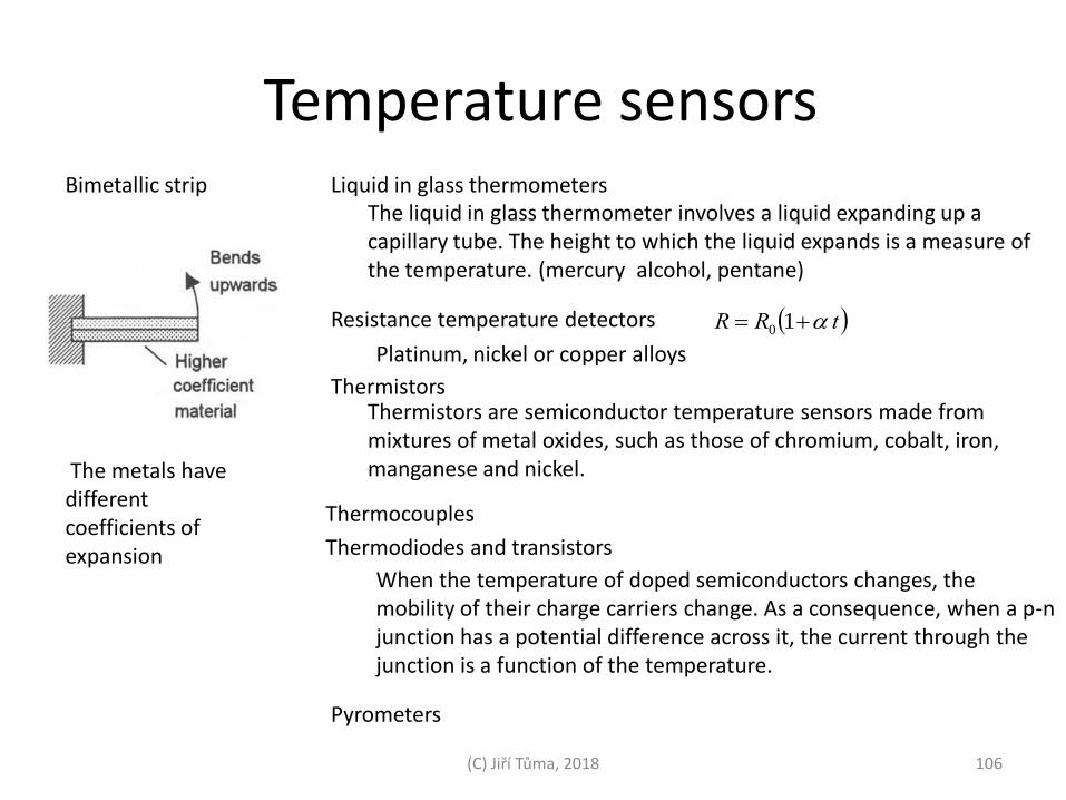
Temperature sensors

(C) Jiří Tůma, 2018 106

Bimetallic strip

The metals have different coefficients of expansion

Liquid in glass thermometers

Resistance temperature detectors

Thermistors

Thermocouples

Thermodiodes and transistors

Pyrometers

The liquid in glass thermometer involves a liquid expanding up a capillary tube. The height to which the liquid expands is a measure of the temperature. (mercury alcohol, pentane)

Platinum, nickel or copper alloys

tRR 10

Thermistors are semiconductor temperature sensors made from mixtures of metal oxides, such as those of chromium, cobalt, iron, manganese and nickel.

When the temperature of doped semiconductors changes, the mobility of their charge carriers change. As a consequence, when a p-n junction has a potential difference across it, the current through the junction is a function of the temperature.

Resistance thermometer

Pt 100 T

Vzdálená

instalace

Pt 100 T

I = konst

Pt 100 T

Four-wire configuration Three-wire configuration Two-wire configuration

Pt – 100, resistance for temperature of 0°C 100 Ω

107 (C) Jiří Tůma, 2018

(alternatively Pt – 500, Pt – 1000)

//upload.wikimedia.org/wikipedia/commons/e/eb/Rtdconstruction.gif

//upload.wikimedia.org/wikipedia/commons/8/80/Coil_Element_PRT.png

Temperature-dependent resistances

(C) Jiří Tůma, 2018 108

Temperature Resistance in Ω

in °C ITS-90 Pt100

Pt100 Pt1000

Typ: 404 Typ: 501

−50 79.901192 80.31 803.1

−40 83.945642 84.27 842.7

−30 87.976963 88.22 882.2

−20 91.995602 92.16 921.6

−10 96.001893 96.09 960.9

0 99.996012 100.00 1000.0

10 103.977803 103.90 1039.0

20 107.947437 107.79 1077.9

30 111.904954 111.67 1116.7

40 115.850387 115.54 1155.4

50 119.783766 119.40 1194.0

60 123.705116 123.24 1232.4

70 127.614463 127.07 1270.7

80 131.511828 130.89 1308.9

90 135.397232 134.70 1347.0

100 139.270697 138.50 1385.0

150 158.459633 157.31 1573.1

200 177.353177 175.84 1758.4

Thermocouples

thermostat 500C

Copper cable

terminals

Hot junction T1 T2

A B voltmeter

Cold junction Properties of thermocouple circuits

Long length of extension cable

Head

Measuring junction Conductors Sheath Insulator

Metal A

Metal B

109 (C) Jiří Tůma, 2018

Material EMF versus temperature

With reference to the characteristics of pure Platinum

emf-electromotive force

110

alloy


Themocouple characteristics table

Class 1 Class 2 Class 3

Thermocouple Range [° C] Tolerance

[° C] Range [°C]

Tolerance [° C]

Range [°C] Tolerance [°C]

T Cu-CuNi -40 to 350 ±0,5 or

±0,004 T -40 to 350

±1,0 or ±0,0075 T

-200 to 40 ±1,0 or ±0,0015 T

E NiCr-CuNi -40 to 800 ±1,5 or

±0,004 T -40 to 900

±2,5 or ±0,0075 T

J Fe-CuNi -40 to 750 ±1,5 or

±0,004 T -40 to 750

±2,5 or ±0,0075 T

K NiCr-Ni -40 to 1000 ±1,5 or

±0,004 T -40 to 1200

±2,5 or ±0,0075 T

-200 to 40 ±2,5 or ±0,0015 T

N NiCrSil-NiSil -40 to 1000 ±1,5 or

±0,004 T -40 to 1200

±2,5 or ±0,0075 T

-200 to 40 ±2,5 or ±0,0015 T

S Pt10Rh-Pt 0 to 1100 (… to 1600)

±1,5 or ±0,004 T

0 to 1600 ±1,5 or ±0,0025 T

R Pt13Rh-Pt 0 to 1100

(… to 1600) ±1 or ±0,004

T 0 to 1100

±1,5 or ±0,0025 T

B Pt30Rh-Pt6Rh 600 to 1700 ±1,5 or ±0,0025 T

600 to 1700 ±4 or ±0,005 T

111 (C) Jiří Tůma, 2018

Installation of thermocouples

Termination head

Nipple

Union

Nipple

112 (C) Jiří Tůma, 2018

Pyrometers

(C) Jiří Tůma, 2018 113

Total radiation pyrometer Disappearing filament pyrometer

Installation of thermocouples

Termination head

Nipple

Union

Nipple

114 (C) Jiří Tůma, 2018

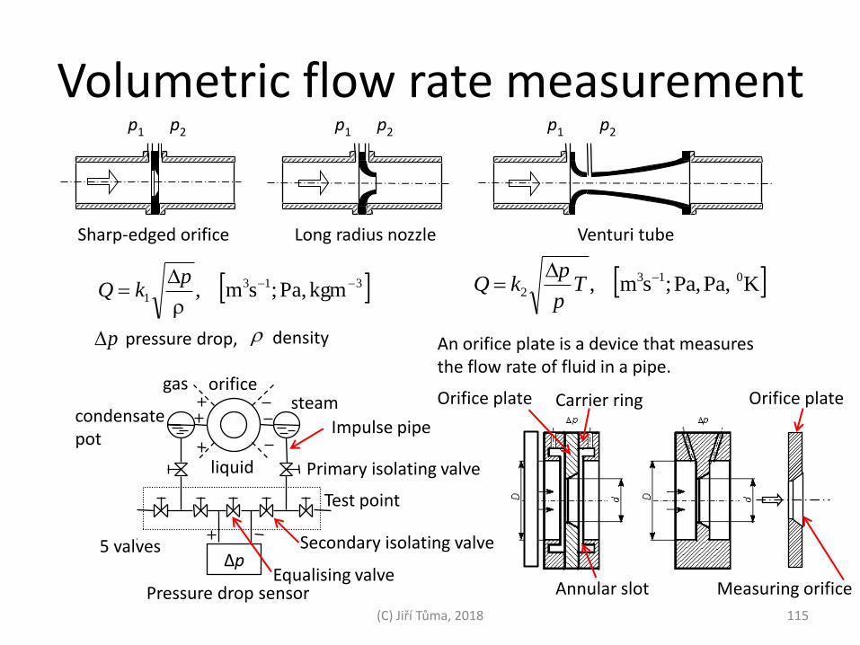
Volumetric flow rate measurement

Sharp-edged orifice

p1 p2 p1 p2

Long radius nozzle

p1 p2

Venturi tube

313

1 kgmPa,;sm,

pkQ KPa,Pa,;sm, 013

2

T

p

pkQ

pressure drop, p density

liquid

Δp

Pressure drop sensor

steam orifice

condensate pot

gas

5 valves

Impulse pipe

Orifice plate Carrier ring

Annular slot Equalising valve

Test point

Primary isolating valve

Secondary isolating valve

An orifice plate is a device that measures the flow rate of fluid in a pipe.

Orifice plate

115

Measuring orifice


Orifice plate installation

Flange

pipe elbow pipe diameter

Orifice plate installation - how much straight pipe should be upstream and downstream?

Flange

DL 101

pipe elbow

DL 51

Orifice

D

upstream downstream

116 (C) Jiří Tůma, 2018

//upload.wikimedia.org/wikipedia/commons/b/b8/Blende_eng.png

//upload.wikimedia.org/wikipedia/commons/0/0f/Orifice.png

http://www.google.cz/url?sa=i&source=images&cd=&cad=rja&docid=ghA3AT6k_ZJ3JM&tbnid=ru4JbNiMY6EdrM:&ved=0CAgQjRwwAA&url=http://cr4.globalspec.com/thread/54623/Seal-pot-for-gas-service&ei=vIY9Uc_VMMnO4QTd5YCABw&psig=AFQjCNGkwAZWGOGoj55RH2Ym8ZYk5aIR2Q&ust=1363073084830807

Flow rate measurement

v

E

N

S B

v Impulse sensor

v

Flow rate is proportional to rotational frequency

Karman effect Magnetic flow meters Turbine flowmeter

Vortex

For a particular bluff body, the number of vortices produced per second, is proportional to the flow rate. For example, a thermistor, heated as a result of a current passing through it, senses vortices due to the cooling effect caused by their breaking away.

bluff body

B magnetic field v velocity L length of conductor E voltage

E = B v L

for conductive process medium Sensing

electrodes

117 (C) Jiří Tůma, 2018

Coriolis mass - flow meters

118 (C) Jiří Tůma, 2018

If a moving mass is subjected to an oscillation perpendicular to its direction of movement, Coriolis forces occur depending on the mass flow. A Coriolis mass flowmeter has oscillating measuring tubes to precisely achieve this effect. Sensors at the inlet and outlet ends register the resultant phase shift in the tube's oscillation geometry. The processor analyzes this information and uses it to compute the rate of mass flow. The oscillation frequency of the measuring tubes themselves, moreover, is a direct measure of the fluids' density.

The vector formula for the magnitude and direction of the Coriolis acceleration Where is the acceleration of the particle in the rotating system, , is the velocity of the particle with respect to the rotating system, and Ω is the angular velocity vector

Actuators

Control valve characteristics

120

Seals Valve plug Valve seat

P1 P2

P1 – P2

Actuator force Stem

pressure pressure

Valve seat

Valve plug

Linear Equal percentage Fast opening

Fluid flow

Stem movement

A B C

Flow through a single seat, two-port globe valve

All control valves have an inherent flow characteristic that defines the relationship between 'valve opening' and flowrate under constant pressure conditions. Valve opening‘ refers to the relative position of the valve plug to its closed position against the valve seat. The orifice pass area is sometimes called the 'valve throat' and is the narrowest point between the valve plug and seat through which the fluid passes at any time.

flowrate

valve opening

Butterfly valve

Ball valve


Valve and actuator configurations

121

Control signal

0-10 V, 4-20 mA

Controller

Manual

Power 230 V 110 V

24 V

Air inlet

Spindle movement with increase in air pressure

Normally open Normally closed

Air inlet

Spindle movement with increase in air pressure

Position transducer

Return spring

Positioning circuit

Feedback potentiometer

Typical electric valve actuator Typical pneumatic valve actuator

http://www.spiraxsarco.com/resources/steam-engineering-tutorials.asp


Pressure drop vs. flow rate

122

P

Q

ΔPline losses

0

ΔPvalve

Ppump head

Q

x

Equal percentage

0

Linear

0

P

Q

ΔPline losses

0

ΔPvalve

Phydrostatic head

0

Q

x

Equal percentage

0

Linear

0

0

Flow rate Flow rate

Pressure drop Pressure drop

Flow rate Flow rate

Stem position (% open) Stem position (% open)

Flow System with Relatively Constant Valve Pressure Drop

The linear globe valve has been designed so that the dependence of the flow rate on the valve opening was linear at a constant pressure drop

The equal percentage globe valve has been designed so that the dependence of the flow rate on the valve opening was linear for an ordinary pump

Pump characteristics

(Pump head is a pump pressure)


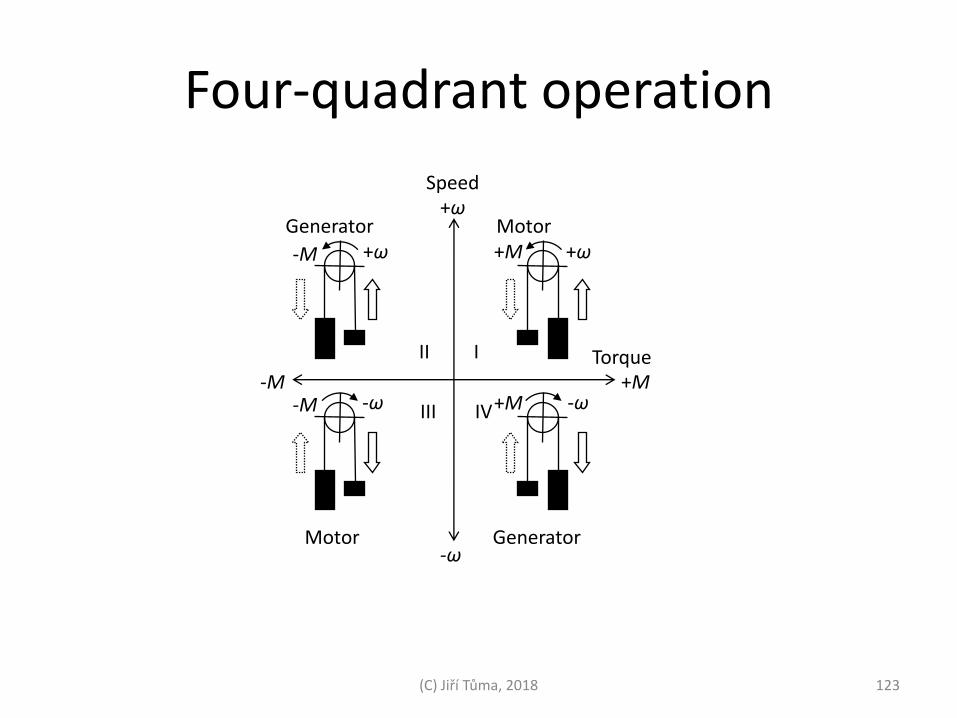
Four-quadrant operation

123

Motor

Motor

Generator

Generator

+M -M

+ω

-ω

I II

IV III

Torque

Speed


+ω +ω

-ω -ω

+M

+M -M

-M

Motion conversion 1

124

circular spline is a rigid circular ring

flex spline

wave generator plug

Ball screw

A ball screw is a mechanical linear actuator that translates rotational motion to linear motion with little friction. A threaded shaft provides a helical raceway for ball bearings which act as a precision screw.

Conversion of rotation to linear motion

Harmonic drive Conversion of high speed rotation to low speed rotation (Strain Wave Gearing )

The advantages: no backlash, light weight, high gear ratios (a ratio from 30:1 up to 320:1 while planetary gears typically only produce a 10:1 ratio), high torque capability, and coaxial input and output shafts.


http://harmonicdrive.de/en/

https://www.youtube.com/watch?v=2shapHAanIU

https://www.youtube.com/watch?v=bzRh672peNk

teeth

internal

external

https://www.youtube.com/watch?v=iRKDfknqtbc

https://www.youtube.com/watch?v=tMh-Axar3o8

//upload.wikimedia.org/wikipedia/commons/8/85/Harmonic_drive_animation.gif

Motion conversion 2

125

outer ring gear or annulus

sun (central gear)

arm or planet carrier

planetary gears

input output

Planetary gearbox

(Epicyclic gears )

Conversion of high speed rotation to low speed rotation

There are three basic components of the epicyclic gear: the sun (a central gear), the planet carrier (holds one or more peripheral planet gears, all of the same size, meshed with the sun gear) and the annulus (an outer ring with inward-facing teeth that mesh with the planet gear or gears). In many epicyclic gearing systems, one of these three basic components is held stationary; one of the two remaining components is an input, providing power to the system, while the last component is an output, receiving power from the system.


//upload.wikimedia.org/wikipedia/commons/d/d5/Epicyclic_gear_ratios.png

Electric motors

Semiconductor power electronics

(C) Jiří Tůma, 2018 127

v i iG iG

u

i

t

t

t

V – I characteristic

iB

iC

vC

B E

C

0 vC 0

iC

iB

iB = 0


Transistor Rvi

BCC ivfi ,

P N

anode catode

Diode symbol v

i


i

v

forward

breakdown

Diode A diode is a two-terminal electronic component with an asymetric characteristic

v i

R

v

t i

Thyristor iA

vA iG

iG = 0

Symbol

A thyristor is a three-terminal electronic component

Rectifier effect Ferdinand Braun discovery 1876

Rectifier effect under control

reverse

vA

iA

gate

catode anode

iG

P N N P

Invented in 1947 by John Bardeen and Walter Brattain

128

Major Categories by Type of Motor Commutation

Self-Commutated Externally Commutated

Mechanical- Commutator Motors

Electronic- Commutator (EC)

Motors

Asynchronous

Machines

Synchronous

Machines2

AC DC AC AC

* Universal motor (AC commutator series Motor or AC/DC motor)1 * Repulsion motor

Electrically excited DC motor: * Separately excited * Series * Shunt * Compound PM DC motor

With PM rotor: * BLDC motor With ferromagnetic rotor: * SRM

Three-phase motors: * SCIM * WRIM AC motors: * Capacitor * Resistance * Split * Shaded-pole

Three-phase motors: * WRSM * PMSM or BLAC motor - IPMSM - SPMSM * Hybrid AC motors: * Permanent-split capacitor * Hysteresis * Stepper * SyRM * SyRM-PM hybrid

Simple electronics Rectifier,

linear transistor(s) or DC chopper

More elaborate electronics

Most elaborate electronics (VFD), when provided


http://en.wikipedia.org/wiki/Brushed_DC_electric_motor

http://en.wikipedia.org/wiki/Universal_motor

http://en.wikipedia.org/wiki/Repulsion_motor

http://en.wikipedia.org/wiki/Brushless_DC_motor

http://en.wikipedia.org/wiki/Switched_reluctance_motor

http://en.wikipedia.org/wiki/Induction_motor

http://en.wikipedia.org/wiki/Wound_rotor_motor

http://en.wikipedia.org/wiki/Shaded-pole_motor



http://en.wikipedia.org/wiki/Synchronous_motor

http://en.wikipedia.org/wiki/Permanent_magnet_synchronous_motor

http://en.wikipedia.org/wiki/Brushless_AC_electric_motor

http://en.wikipedia.org/wiki/Stepper_motor

http://en.wikipedia.org/wiki/Reluctance_motor

http://en.wikipedia.org/wiki/Variable-frequency_drive

Direct current (DC) electric motor analysis

129

Brushed DC electric motor

Split ring commutator

A brushed DC electric motor generates torque from DC power supply by using internal mechanical commutation, permanent magnets form the stator field. Torque is produced by the principle of Lorentz force, which states that any current-carrying conductor placed within an external magnetic field experiences a force known as Lorentz force.

Permanent magnet

I

R

V

IRVR

kE

IkM ,

M

Increase of V

Decrease of

MBA

M

k

R

k

V

k

kMRV

k

IRV

k

E

2

Carbon brushes

Rotational velocity

Torque

Armature resistsance

Internally generated voltage (EMF)

Armature current

Terminal voltage

Constant based upon motor construction

R

E

I

V

k

M

Magnetic flux in motor coils

Power supply

A basic equation of a DC motor:

How to control rotational velocity + by changing terminal voltage

+ by changing magnetic flux.

Armature


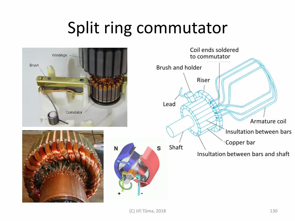
Split ring commutator

130

Shaft

Lead

Riser

Brush and holder

Coil ends soldered to commutator

Armature coil

Insultation between bars

Copper bar

Insultation between bars and shaft


http://www.google.cz/url?sa=i&rct=j&q=dc+motor&source=images&cd=&cad=rja&docid=uxrFBCiE5M-zVM&tbnid=7PceZ7MkbNosbM:&ved=0CAUQjRw&url=http://www.submarineboat.com/rov_joystick_for_props.htm&ei=3D1KUbzHPISOtQbL5IC4CQ&bvm=bv.44011176,d.Yms&psig=AFQjCNHL_9kjT-Q9ifqSsOY2lYqKwnB7VA&ust=1363904466062800

http://en.wikipedia.org/wiki/File:Electric_motor.gif

http://www.google.cz/url?sa=i&rct=j&q=commutator&source=images&cd=&cad=rja&docid=gauS_lh7MjV4GM&tbnid=eN3zsAhlrUcvTM:&ved=0CAUQjRw&url=http://www.answers.com/topic/commutator&ei=mFFNUY3INIWdtAah_YDQCA&bvm=bv.44158598,d.bGE&psig=AFQjCNHNhmNgeXm0vqKWt_e5MQM553gLWQ&ust=1364107645011020

Brushed DC motors

131

IB1

ω, M

AM G M

IB2

3 x U1

Ward Leonard motor control system

Permanent magnet DC motor

Wound stators - Electrically excited DC motor

series compound shunt

field coil field coil

field coil

field coil field coil

3 x V1 G generator, M motor

AM asynchronous motor

Grid


How to choose a flyback diode for a relay?

132

https://electronics.stackexchange.com/questions/110574/how-to-choose-a-flyback-diode-for-a-relay


A diode is put in parallel with a relay coil (with opposite polarity) to prevent damage to other components when the relay is turned off.

First determine the coil current when the coil is on. This is the current that will flow through the diode when the coil is switched off. In your relay, the coil current is shown as 79.4 mA. Specify a diode for at least 79.4 mA current. In your case, a 1N4001 current rating far exceeds the requirement. The diode reverse voltage rating should be at least the voltage applied to the relay coil. Normally a designer puts in plenty of reserve in the reverse rating. A diode in your application having 50 volts would be more than adequate. Again 1N4001 will do the job. Additionally, the 1N4007 (in single purchase quantities) costs the same but has 1000 volt rating.

DC electric motor control

133

time

Voltage Average: high

Average: medium

Average: low

Pulse width modulation (variable duty cycle)

Optical chopper

PID Controller

Pulse width modulator

Feeback

Error DC motor

Frequency to voltage converter

Set point

Tacho

DC motor

Switching transistor or MOSFET

Flyback (kickback) diode

Logic control


D T

Period Duty cycle … D / T = ξ

0

0

d Uttuu

T

u(t) U0

U0

U0

u(t)

u(t)

A chopper is an electronic switch that is used to interrupt one signal under the control of another

Voltage mean value …

Duty cycle

http://www.google.cz/url?sa=i&rct=j&q=dc+motor&source=images&cd=&cad=rja&docid=D6CUWeflnT3gIM&tbnid=f0r4DWfi9Z4UOM:&ved=0CAUQjRw&url=http://emadrlc.blogspot.com/2012/07/dc-motor-field-structure-and-armature.html&ei=nldNUZqVCYPNtAbcroDACA&bvm=bv.44158598,d.Yms&psig=AFQjCNGyzhw8EV0t-c1iU3oQx1qa0HQAaQ&ust=1364109563219499

Chopper (electronics)

(C) Jiří Tůma, 2018 134

In electronics, a chopper circuit is used to refer to numerous types of electronic switching devices and circuits used in power control and signal applications. A chopper is a switching device that converts fixed DC input to a variable DC output voltage directly. A chopper is an electronic switch that is used to interrupt one signal under the control of another. In signal processing circuits, use of a chopper stabilizes a system against drift of electronic components; the original signal can be recovered after amplification or other processing by a synchronous demodulator that essentially un-does the "chopping" process.

An inverter changes a DC input to an AC output

Three-phase electricity

(C) Jiří Tůma, 2018 135

Three-phase transformer. Each phase has its own pair of windings

Three-phase electric power systems have at least three conductors carrying alternating current voltages that are offset in time by one-third of the period.

230/400V system provides 230V between the neutral (centre hub) and any one of the phases, and 400V across any two phases.

//upload.wikimedia.org/wikipedia/commons/c/cc/3_phase_AC_waveform.svg

//upload.wikimedia.org/wikipedia/commons/e/e1/Transformator-3-fas.png

Induction motors

136

An induction or asynchronous motor is an AC motor in which all electromagnetic energy is transferred by inductive coupling from a primary winding to a secondary winding, the two windings being separated by an air gap. In three-phase induction motors, that are inherently self-starting, energy transfer is usually from the stator to either a wound rotor or a short-circuited squirrel cage rotor.

Stator

Rotor

3 x U Odpory

Squirrel cage rotor Wound rotor motor

The rotor windings of this motor are connected through slip rings to external resistances. Adjusting the resistance allows control of the speed/torque characteristic of the motor.

Stator

Wound Rotor

External rotor resistance

3 x V1

Cutaway view

The rotor is comprised of a number of thin bars, usually aluminum, mounted in a laminated cylinder.

Conductor bars

End ring

Brushes

Slip rings


//upload.wikimedia.org/wikipedia/commons/6/65/Schleifringl%C3%A4ufer.svg

//upload.wikimedia.org/wikipedia/commons/a/a9/Rotterdam_Ahoy_Europort_2011_(14).JPG

Stator and rotor windings

137

http://textiletechinfo.com/spinning/induction-motor-3.htm

To phase A

To phase A

Magnetic field of coil A1

Stator

Rotor

Rotor conductor bars


Cage induction motor rotor's conductor bars are typically skewed to reduce noise

Number of poles per phase

138

http://textiletechinfo.com/spinning/induction-motor-3.htm

The number of poles is determined by how many times a phase winding appears.

2-Pole stator winding

A three-phase power supply provides a rotating magnetic field in an induction motor.

22 1

0p

f

Synchronous speed 0

1f pp

2p

where is the motor supply's frequency in Hertz and is the number of magnetic poles. That is, for a two-pole three-phase motor with three pole-pairs set 120° apart, equals 2 and equals 3 000 RPM for 50 Hz supply systems. is the number of pole pairs.

Example

0° 60° 120° 180° 240°

Rotation angle in deg

360° 300°


(A1 and A2)

2/p

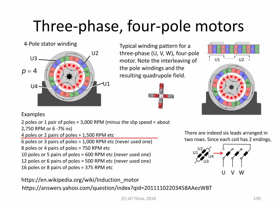
Three-phase, four-pole motors

139

https://answers.yahoo.com/question/index?qid=20111102203458AAezWBT

https://en.wikipedia.org/wiki/Induction_motor

4-Pole stator winding

4p


U1

2 poles or 1 pair of poles = 3,000 RPM (minus the slip speed = about 2,750 RPM or 6 -7% ns) 4 poles or 2 pairs of poles = 1,500 RPM etc 6 poles or 3 pairs of poles = 1,000 RPM etc (never used one) 8 poles or 4 pairs of poles = 750 RPM etc 10 poles or 5 pairs of poles = 600 RPM etc (never used one) 12 poles or 6 pairs of poles = 500 RPM etc (never used one) 16 poles or 8 pairs of poles = 375 RPM etc

U2 U3

U4

Typical winding pattern for a three-phase (U, V, W), four-pole motor. Note the interleaving of the pole windings and the resulting quadrupole field.

U1 U2

Examples

There are indeed six leads arranged in two rows. Since each coil has 2 endings,

U V W

U1 U2

U3 U4

Speed – torque characteristics

140

0

1

s

The rotating magnetic flux induces currents in the windings of the rotor.

Slip, s, is defined as the difference between synchronous speed ω and operating speed ω0 , at the same frequency, expressed in rpm or in percent or ratio of synchronous speed.

How to control rotational velocity

+ by changing slip (wound rotor motor)

+ by changing frequency

+ by changing the number of poles

+ by changing voltage

Speed (ω) - torque (T) curves for four induction motor types: A) Single-phase, B) Polyphase cage, C) Polyphase cage deep bar, D) Polyphase double cage.

T

T

T

T

ω ω

ω ω

T T

ω ω

changing voltage changing slip


//upload.wikimedia.org/wikipedia/commons/a/ad/Torque_electric_motor_AC.svg









Star (wye) and delta connection of the 3-phase squirrel-cage induction motors

(C) Jiří Tůma, 2018 141

L1 L2 L3 L1 L2 L3

L1 L2 L3 L1 L2 L3 Delta connection Star connection (Y configuration)

Grid

When an induction motor is started directly on line, it takes a starting current 6(six) times the full load current. To reduce the starting current the voltage across the motor need to be reduced. This can be done by autotransformer starter, star-delta starter or resistor starter. For star-delta connection the motor windings are connected in star (Y) during starting. The connection is changed to delta when the motor starts running.

Grid

NLLL UU 3LLU NLU

The voltage between line conductors is √3 times the phase conductor to neutral voltage:

Two windings per phase

Only one winding per phase

For star configuration the winding is powered by √3 times reduced voltage. The power consumption (proportional to UL-N square) is 3 times reduced.

LLU

Connection box

bridging

Connection box

http://www.electricneutron.com/wp-content/uploads/2011/04/motor-terminal-voltage.jpg

http://www.electricneutron.com/wp-content/uploads/2011/04/delta-connection.jpg

//upload.wikimedia.org/wikipedia/commons/9/9e/The_basic_3-phase_configurations.svg

//upload.wikimedia.org/wikipedia/commons/9/9e/The_basic_3-phase_configurations.svg

Controlled rectifiers

142

3 x U1

AC DC

Diode Transformer

Three-phase bridge rectifier

Half wave rectifier

Full-wave rectifier using 4 diodes

Three-phase full-wave rectifier circuit using thyristors as the switching elements, with a center-tapped transformer

Grid

Grid

Three-phase supply Single-phase supply

R

R

Thyristors

AC DC

Average


3 x U1

Full-wave rectifier using a center tap transformer and 2 diodes

peakDC UU

peakDC UU 2Primary winding

Secondary winding

Thyristors

peakDC UU 2

Single phase Triple phase

//upload.wikimedia.org/wikipedia/commons/5/58/Halfwave.rectifier.en.svg

//upload.wikimedia.org/wikipedia/commons/d/d5/Gratz.rectifier.en.svg

http://en.wikipedia.org/wiki/File:Fullwave.rectifier.en.svg

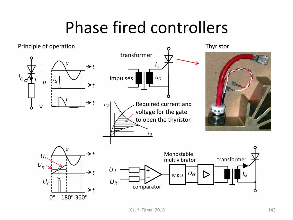
Phase fired controllers

143

u i iG iG

u

i

t

t

t

transformer

impulses

iG

uG

i G

u G

Principle of operation

transformer

comparator

I G MKO

U R

U I U G

Monostable multivibrator

Thyristor

UG

u

UI t

t

t 0° 180° 360°

UR

Required current and voltage for the gate to open the thyristor


//upload.wikimedia.org/wikipedia/commons/5/56/SCR1369.jpg

Transistor as a switch

144

3 x U U

1 R B

T 1

T 2

T 3

T 4

AM

C

T 5

T 6

IA IC

IB

IA

IB

IC

time

iB = 0

R

iBMax

R

AM

0 uC U0 0

iC

U0 R

iB

iBMax

iB = 0


ON

OFF

t

t

t

t

t

UZ

iB

iZ

iT

iD

iZ0

iZ1

iZ0

period

pulse

= =

iB

iZ

iD

UZ

U

iT R L E

Pulse width modulation

*) When a coil is switched off, a large BACK EMF of several thousand volts in value appears across the coil.


CC uiRU 0RuRUi CC 0

IA

IC

IB

(variable duty cycle) R iC U0

uC

open

closed

A flyback (snubber, freewheeling, suppressor, or catch) diode eliminates a sudden voltage spike.

Diode protection circuit *)

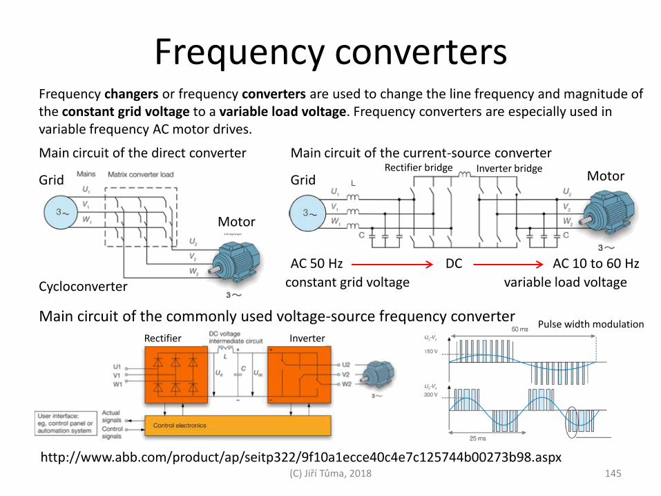
Frequency converters

145

http://www.abb.com/product/ap/seitp322/9f10a1ecce40c4e7c125744b00273b98.aspx

Frequency changers or frequency converters are used to change the line frequency and magnitude of the constant grid voltage to a variable load voltage. Frequency converters are especially used in variable frequency AC motor drives.

Grid Grid

Motor

Motor

Main circuit of the direct converter Main circuit of the current-source converter

Cycloconverter

AC 50 Hz DC AC 10 to 60 Hz

Main circuit of the commonly used voltage-source frequency converter

constant grid voltage variable load voltage



Rectifier Inverter

Rectifier bridge Inverter bridge


146

https://en.wikipedia.org/wiki/Pulse-width_modulation

A simple method to generate the PWM pulse train corresponding to a given signal is the intersective PWM: the signal (here the red sinewave) is compared with a sawtooth waveform (blue). When the latter is less than the former, the PWM signal (magenta) is in high state (1). Otherwise it is in the low state (0).


Time

lead

ing

edge

tr

ailin

g ed

ge

bo

th

edge

s

Time

PW

M s

ign

al

Sin

uso

idal

sig

nal

Stepper motors

147

+

Coil 1

Coil 3

T 1

T 2

T 3

T 4

Coil 2

Coil 4

4

T 1

T 2

+

Coil 1 Coil 3

T 4

T 3

T 5

T 6

Coil 2 Coil 4

T 8

T 7

-

4

Unipolar Transistor Switch

There are three basic types of stepper motor, Variable Reluctance (plain iron rotor which operate based on the principle that minimum reluctance occurs with minimum gap), Permanent Magnet and Hybrid (a sort of combination of both). A Stepper Motor is particularly well suited to applications that require accurate positioning and speed control

Two bi-directional H-bridge Circuits

3-Phase stator

Shaft bearing

Magnetic shaft

Rotor poles Stator coils

Bearing housing

Stator poles

Active winding

4-Phase stator

Multi-toothed magnetic rotor


2

1

http://www.google.cz/url?sa=i&rct=j&q=stepper+motor&source=images&cd=&cad=rja&docid=X-siCS90XnIN5M&tbnid=wEbLT31_2N2vqM:&ved=0CAUQjRw&url=http://www.engineersgarage.com/articles/stepper-motors?page=2&ei=mehNUe-GFMrMtQbF-oGwBg&bvm=bv.44158598,d.bGE&psig=AFQjCNEgUvgyvYTBgA1XFbaLcNn4dBn1uQ&ust=1364146539464269

http://www.google.cz/url?sa=i&rct=j&q=stepper+motor&source=images&cd=&cad=rja&docid=X-siCS90XnIN5M&tbnid=wEbLT31_2N2vqM:&ved=0CAUQjRw&url=http://www.electronics-tutorials.ws/io/io_7.html&ei=zOlNUem-DIrRsgbR1ICwDw&bvm=bv.44158598,d.bGE&psig=AFQjCNEgUvgyvYTBgA1XFbaLcNn4dBn1uQ&ust=1364146539464269

http://www.google.cz/url?sa=i&rct=j&q=stepper+motor&source=images&cd=&cad=rja&docid=X-siCS90XnIN5M&tbnid=wEbLT31_2N2vqM:&ved=0CAUQjRw&url=http://www.engineersgarage.com/articles/stepper-motors?page=2&ei=mehNUe-GFMrMtQbF-oGwBg&bvm=bv.44158598,d.bGE&psig=AFQjCNEgUvgyvYTBgA1XFbaLcNn4dBn1uQ&ust=1364146539464269

Hydraulic actuators

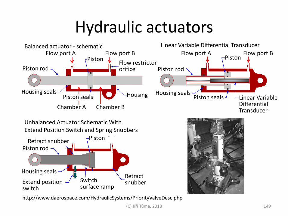
Hydraulic actuators

149

Balanced actuator - schematic

Piston rod

Housing seals

Flow restrictor orifice

Piston

Housing

Flow port B Flow port A

Chamber A Chamber B

Piston seals Housing seals

Piston seals

Piston Flow port B Flow port A

Piston rod

Linear Variable Differential Transducer

Piston

Piston rod

Housing seals Retract snubber

Retract snubber

Switch surface ramp

Extend position switch

Linear Variable Differential Transducer

Unbalanced Actuator Schematic With Extend Position Switch and Spring Snubbers

http://www.daerospace.com/HydraulicSystems/PriorityValveDesc.php


Hydraulic motors

150

Axial piston hydraulic motor

Gear Hydraulic Motor


Outlet (to reservoir)

Inlet (from system)

Motor shaft

Pistons

Vanes (spring loaded) Vane slot

Cam ring

Inlet

Outlet

Gear Gear

Output shaft Input shaft

Outlet Inlet

Rotor Shaft

There are 3 main types of hydraulic motors: piston, vane and gear.

Rotating Stationary

Swashplate does not rotate

Principle


Inlet (from system)

Motor shaft


Vane Hydraulic Motor

Direction of rotation

part part

variable

Piston pump and motor unit (Uni-directional)

151

Piston pump Piston motor


Pistons

Rotating Stationary

Swashplate does not rotate Outlet (to

system)

Inlet (from reservoir) Pump/Motor

shaft

Pistons

Rotating Stationary


Inlet (from system)


Inlet (from system)

Outlet (to system)

Inlet (from reservoir)

Compensator

Variable


Compensator

Piezoactuators

Piezoelectric effect

Domain Dipole Mechanical stress

Mechanical stress

Electric field Electric

voltage +

-

The behavior of the piezoelectric material in the unpolarized state (left) polarization after mechanical compression (middle), and after insertion of polarization of piezoelectric material to an electric field (right)

Direct piezoelectric effect discovered the brothers Pierre and Jacques Curie. They found that certain crystalline materials (ceramics) having the ability to polarize when subjected to an external force. Mechanical stress (compression and tension) generates electric charge and the electric field and external force in proportion. This phenomenon is used in sensors for dynamic forces. The inverse phenomenon lies in the fact that the electric field that is oriented parallel to the polarization direction, excites the mechanical expansion or contraction of the material. Piezoelectric effect is anisotropic, ie they act only in a certain direction.

153 (C) Jiří Tůma, 2018

Piezoelectric coefficients and directions

polarization

1

2

3

4

5

6 dij: Strain coefficients [m/V]:

strain developed (m/m) per electric field applied

(V/m) or (due to the sensor / actuator properties of

Piezo material). Charge output coefficients [C/N]:

charge density developed (C/m²) per given stress

(N/m²).

gij: Voltage coefficients or field output coefficients

[Vm/N]:

open circuit electric field developed (V/m) per

applied mechanical stress (N/m²) or (due to the

sensor / actuator properties of Piezo material) strain

developed (m/m) per applied charge density (C/m²).

kij: Coupling coefficients [no Dimensionss].

The coefficients are energy ratios describing the

conversion from mechanical to electrical energy or

vice versa

Example: d33 applies when the electric field is along the polarization axis (direction 3) and the strain (deflection) is along the same axis. d31 applies if the electric field is in the same direction as before, but the strain is in the 1 axis (orthogonal to the polarization axis)

http://www.physikinstrumente.com/tutorial/4_16.html

i – strain direction j – polarization direction

154 (C) Jiří Tůma, 2018

Piezoelectric materials The most popular material is a piezoelectric ceramic PZT (Lead-Zirconate-titanate) or polymer PVDF (Polyvinilidene fluoride).

Material PZT PVDF Piezoelectric coefficients d33 (10-12 C/N or m/V) d31 (10-12 C/N or m/V)

300 -150

-25

uniaxial d31=15 d32=3 biaxial

d31=d32==3

Maximum stress (MPa) Tensile stress Compression

600 80

200 200

Maximum intensity of the electric field (V/mm) 2000 5.105

Density (kg/m3) 7600 1800

155 (C) Jiří Tůma, 2018

Piezoactuator types Three types of piezoelectric actuators are reported in literature

Linear piezoelectric actuator

Linear motor

o Inchworm motors

o Stick and slip actuators

o Traveling wave ultrasonic motors

Piezoelectric benders

156 (C) Jiří Tůma, 2018

Linear piezoelectric actuators Displacement of piezoelectric actuators

ΔL

L U

1

2

n

Piezoelectric stack

ΔL

L U

t 313 dLEL

nUdL 33

Laminar piezoactuator

157 (C) Jiří Tůma, 2018

http://www.google.cz/url?sa=i&rct=j&q=piezo+stack+actuator&source=images&cd=&cad=rja&docid=ZxgVUqTOx08QyM&tbnid=w754ehXznVcyYM:&ved=0CAUQjRw&url=http://www.piceramic.com/site/stack.html&ei=QRBQUcrdJ8eVswaUgoGQCw&bvm=bv.44158598,d.Yms&psig=AFQjCNFyLi_jMStGM9UfoflG-blOej5gdw&ust=1364284549670571

Diamond piezoactuators

(C) Jiří Tůma, 2018 158

Blocking force [N]

Free stroke [μm]

Output member Piezoelectric actuator

Fixed member Actuator pair

Tension member

Plate benders

Ring benders

Stacked actuator

Single actuator

Wire

Noliac piezo

10000

1000

100

10

1

0.1 1 10 100 1000 10000 100000 0.1

http://www.google.cz/url?sa=i&rct=j&q=piezo+stack+actuator&source=images&cd=&cad=rja&docid=sXwFGWKZnh9J4M&tbnid=ArEpJyN2oKKpQM:&ved=0CAUQjRw&url=http://www.sciencedirect.com/science/article/pii/S0888327007001951&ei=FgNQUaCnM43KtAaL2oHYBA&bvm=bv.44158598,d.Yms&psig=AFQjCNFyLi_jMStGM9UfoflG-blOej5gdw&ust=1364284549670571

Applications piezoactuator

U

Active members in the Pratt truss with piezoactuators

159 (C) Jiří Tůma, 2018

Simple lever-arm mechanism

http://www.google.cz/url?sa=i&rct=j&q=piezo+stack+actuator&source=images&cd=&cad=rja&docid=UEM5ouU7eIv1UM&tbnid=gzq1cJXJMyWRpM:&ved=0CAUQjRw&url=http://rotorcraft.mae.carleton.ca/index.php?page=people/fdu&ei=Ag5QUaTqI4rAtAaRoYGwCQ&bvm=bv.44158598,d.Yms&psig=AFQjCNFyLi_jMStGM9UfoflG-blOej5gdw&ust=1364284549670571

Piezoactuator design Stack actuator – ceramic plates

Two designs of piezoactuators:

Some piezoactuator are designed for open-loop positioning tasks. They have only the voltage input

Closed loop piezoactuator with the voltage input and the SGS-position sensors.

Thickness 0,1 mm ….. 100 V, LVPZ - Low voltage piezo Thickness 1 mm ….. 1000 V, HVPZ - High voltage piezo

The maximum relative displacement is between 0,1 and 0,13 %, what means that the actuator of the 100 mm length has the absolute travel of 100 μm. The hysteresis of piezoactuators is up to 15%.

Blocking force

Travel

Direction of

increasing voltage

0 0

Catalogue parameters

travel (free stroke)

force (blocking)

160 (C) Jiří Tůma, 2018

Products of Physic Instrument company Linear piezoelectric actuator E-504 Piezo Amplifier

Module E-509 Signal Conditioner / Piezo Servo Module

161 (C) Jiří Tůma, 2018

http://www.physikinstrumente.com/en/products/primages.php?sortnr=101000&picview=1

Piezoactuators of the P-844 / P-845 type

Outstanding Lifetime Due to PICMA® Piezo Ceramic Stacks

Travel Range to 90 µm Pushing Forces to 3000 N Pulling Forces to 700 N Sub-Millisecond Response,

Sub-Nanometer Resolution Vacuum Version, Optional

Water-Resistant Case

162 (C) Jiří Tůma, 2018

Technical Data

163 (C) Jiří Tůma, 2018

Movable bushing for a sleeve bearing

(C) Jiří Tůma, 2018 164

Flexible tip

Active vibration control

(C) Jiří Tůma, 2018 165

0 5 10 15 20 25 -300-250

-200-150

-100-100

-300

-250

-200

-150

-100

X [micrometer]

Time [s]

Y [m

icro

me

ter]

Load

Journal position

Reference

Piezoelectric actuators

Rotor system

Controller

dSpace

Proximity probes

Amplifier

Bushing

Piezo actuator drive (PAD)

(C) Jiří Tůma, 2018 166

Kinematic principle with microtoothing

Noliac piezo

Siemens

Slow and precise motion /0 to 60 RPM)

High-speed piezo motor actuators

(C) Jiří Tůma, 2018 167

•Drive-Component for Integration into Automation & Positioning Systems •Flexible Choice of Travel Ranges to Several 100 mm •Flexible Choice of Push/Pull Forces to Several 10 N •Minimum Incremental Motion to 0.05 µm •Velocity to 400 mm/s •Self-Locking w/o Head Build Up

PI M-674 RodDrive: Integrated High-Speed Piezo Motor Actuator

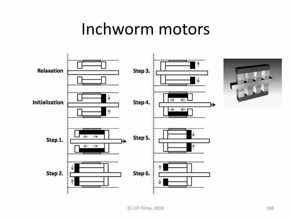
Inchworm motors

168 (C) Jiří Tůma, 2018

Stick and slip actuators

Moving object

Seismic mass

piezo

Moving object

Seismic mass

piezo

Moving object

Seismic mass

piezo

Slow extension

Initial position

Rapid contraction Δx

169 (C) Jiří Tůma, 2018

80-Pitch Screw Starting position

Slow rising

Quick return to starting position

Jaws

Piezo

Thank you for your attention

Symbols in a hydraulic schematic

171 (C) Jiří Tůma, 2018

Lines Square

Continuous line - for flow line One square - pressure control function

Dashed line - for pilot, drain Two or three adjacent squares - directional control

Envelope - for dashes around component symbols

Triangle

Circular Solid - Direction of Hydraulic Fluid Flow

Large Circle - pump, motor Open - Direction of Pneumatic flow

Small Circle - measuring devices Diamond

Semi-circle - rotary actuator Diamond - Fluid conditioner (filter, separator, lubricator, heat exchanger)

Flow restriction

Spring

Symbols in a hydraulic schematic




3 position – 4 way valve Closed Center Valve

Valve capable infinite positioning (indicated by horizontal lines drawn parallel to the envelope

Valves

check valve

On-Off manually shunt off

Valve actuator

spring

solenoid

manual

Single acting

Cylinders

Double acting single rod end

Double acting double rod end

Liquid supply


Hydraulic pump fixed displacement

Reservoir open to atmosphere

172 (C) Jiří Tůma, 2018

Open Center Valve

Cylinders

controllers sensors actuatorshomel.vsb.cz/~tum52/publications/controllers-sensors-actuators.pdf ·...

Documents