coopetition strategy and pricing timing in an outsourcing supply … · 2019-01-10 · coopetition...

1063-6706 (c) 2018 IEEE. Personal use is permitted, but republication/redistribution requires IEEE permission. See http://www.ieee.org/publications_standards/publications/rights/index.html for more information.

This article has been accepted for publication in a future issue of this journal, but has not been fully edited. Content may change prior to final publication. Citation information: DOI 10.1109/TFUZZ.2018.2821106, IEEETransactions on Fuzzy Systems

1

Coopetition Strategy and Pricing Timing in anOutsourcing Supply Chain with Uncertain

Operation RisksHuiru Chen, Yingchen Yan, Nana Ma and Lu Yang

Abstract—At present, an increasing number of original equip-ment manufacturers (OEMs) often outsource their product man-ufacturing to original design manufacturers (ODMs) that alsoproduce their own-brand products and then become powerfulcompetitors of the OEMs. Following this, our work exploreswhether two such direct competitors should still cooperatein their original contract manufacturing and how coopetitiondecisions affect their preferred pricing timing when they enterthe downstream product market. We establish a multi-stagemodel including an OEM and its competitive ODM and derivesome managerial insights. First, we find that the OEM and thecompetitive ODM prefer to cooperate in contract manufacturingas the OEM is more risk loving, the competitive ODM is morerisk averse and the wholesale price is relatively small. Second,we illustrate that the two parties are more likely to achievean agreement on cooperation in the ODM-pricing-early gamerelative to the two other games. Third, we show that whenthe OEM is sufficiently risk averse, the two parties’ preferencesfor pricing timing remain the same regardless of whether theycooperate in contract manufacturing. However, once the OEMbecomes risk loving, it will be less willing to move later asthe wholesale price increase, which is different from classicalBertrand competition.

Index Terms—Uncertain multi-stage decision making; Oper-ation outsourcing; Pricing sequence decision; Confidence level;Uncertainty environment

I. INTRODUCTION

With the rapid development of the economy and business,an increasing number of original equipment manufacturers(OEMs) have begun to outsource their production manufac-turing and even some design functions to original designmanufacturers (ODMs), the contract manufacturers (CMs) thatdesign and manufacture the specified products. For instance,Apple signed contracts with various ODMs, including Quanta,Asus, and Flextronics, with respect to its product manufactur-ing and, partially, its notebook innovations [34]. Moreover,PalmOne outsourced to HTC, a Taiwan-based ODM, thedesign and manufacturing of its popular Treo 650 smartphones[14]. By 2011, the profit earned from the outsourcing business

This work was supported by the National Natural Science Foundationof China under Grant No. 71771165, and the Technological InnovationFoundation in Soft Science Research Project of Hubei Province under GrantNo. 2018ADC083 (Corresponding author: Yingchen Yan and Nana Ma).

Huiru Chen is with the College of Mathematics and Physics, HuanggangNormal University, Hubei 438000, China (e-mail: [email protected]).

Yingchen Yan is with the College of Management and Economics, TianjinUniversity, 300072, China (e-mail: [email protected]).

Nana Ma and Lu Yang are with the School of Statistics, Xi’an Uni-versity of Finance and Economics, Shaanxi 710100, China (e-mail: [email protected]; [email protected]).

had reached 323.9 billion dollars, an increase of 63.6% [7].Through an outsourcing strategy, the OEMs can fully apply ex-terior resources, improve the quality of production and service,shorten production cycles and reduce acquisition costs, therebymaintaining their core competence in a changing economicenvironment.

While an outsourcing strategy benefits the OEMs greatly,it also brings some potential damage at the same time. Asreported by [37], along with handling more outsourcing tasks,the ODMs develop enhanced production capabilities and thenstart to launch their own-brand products that are increasinglysimilar to those of the OEM because the two kinds of productsare produced simultaneously by the same manufacturer usingsimilar production technologies. In this way, the ODM willdirectly seize part of the OEM’s product market and thenbecome their primary downstream competitors. For example,in the consumer electronics industry, HTC, the ODM forGoogle, produces its self-branded HTC Desire smartphone andthe Google Nexus One smartphone, both of which have similarspecifications [38]. Furthermore, considering the ODM’s ad-vantage in manufacturing, consumers in some local emergingmarkets may come to prefer the self-branded products of thecompetitive ODMs over those of the OEMs, which furtherhurts the OEM. For instance, Taiwan-based TPV Technologyproduces products such as computer monitors and LCD tele-visions for Samsung, Sony, and others and produces its ownbrand of products under AOC, which was officially rankedfirst in the Asia-Pacific area [21]. In addition, Asus not onlymanufactured notebooks for its OEMs but also produced itsown self-branded notebook that occupied a market share of12.5% in China [49]. The increased competitiveness of theODMs gives rise to a great threat to the OEMs. Therefore,whether the OEM should outsource to a competitive ODM andwhether a powerful ODM should manufacture for its OEMsbecome especially intriguing questions that are worth studying.

Another problem the OEM and its competitive ODM shouldconsider is timing of pricing when the firms enter the down-stream product market. Generally, under classical Bertrandprice competition, the latter mover often has an advantagebecause the firm can undercut the price of the former moverso as to occupy a larger market share. Nevertheless, oncethe OEM and the competitive ODM cooperate in contractmanufacturing, it is not easy to see whether this intuition canstill hold. In such a setting, they are not only competitorsbut also partners. The competitive ODM needs to balance itsprofit from contract manufacturing and that from the sales



2

of his own-brand products, which will directly affect hisincentive to undercut the other’s price and thus impact thefinal equilibrium timing. Therefore, the following questionalso arises: what are the OEM’s and the competitive ODM’srespective timing preferences? Additionally, what is the finalequilibrium timing?

Moreover, when considering these problems, the firms can-not ignore the risks in the process of outsourcing operations.As shown in an international business report by researchers atOxford University and Missouri University, more than 35% ofoutsourcing trade fails in the end [32]. The Garterne Groupalso reported that the majority of outsourcing failures arethe result of inappropriate decisions and mis-estimated risklevels [7]. In the real world, various types of risks exist inthe outsourcing business. A product’s demand usually hasa high degree of uncertainty and fluctuates in some indus-tries, including the medical device, pharmaceutical, and first-generation PC Markets (Liu 2005). This uncertainty and riskfurther increase the difficulty for the OEM and the competitiveODM in determining their coopetition strategies and pricingtiming.

To adress these above-mentioned questions, we establisha multi-stage model in which the OEM outsources one partof manufacturing to the competitive ODM and the other topart to the non-competitive ODM. The competitive ODM notonly finishes the outsourcing orders from the OEM but alsoproduces her own-brand products that are in competition withproducts of the OEM. Our works primarily focus on the impactof the operation risk and uncertain demand by considering theexternal demand and the product substitution rate as uncertainvariables and by applying the confidence level in uncertaintytheory to characterize the OEM’s and the ODM’s risk attitudes.Specifically, a high confidence level indicates a conservativeattitude, and a low confidence level implies a risk-lovingattitude. Then, we present two situations, one in which theOEM and competitive ODM do not cooperate in contractmanufacturing and another in which they cooperate in contractmanufacturing. Further, in each situation, the OEM and thecompetitive ODM can choose the simultaneous game, theOEM-pricing-early game and the ODM-pricing-early game.Thus, six cases exist here. After maximizing and comparingthe participants’ profits under their respective acceptable con-fidence levels, we obtain the following main insights.

First, we find that the OEM and the competitive ODMprefer to cooperate in contract manufacturing as the OEM ismore risk loving, the competitive ODM is more risk adverseand the wholesale price is relatively small. This result isbecause that, through cooperation with the ODM, the OEMalleviates the aggressive attitude of the competitive ODMwhen they both sell products to the market. Otherwise, whenthe wholesale price is too high, the ODM’s focus will shiftto earning profit from contract manufacturing. This distortedfocus reduces the incentives of the firms to cooperate. Second,we find the two parties are more likely to achieve an agreementon cooperation in the ODM-pricing-early game among thethree games. At this time, the first-mover ODM will considerthe response of the follower OEM, and will then becomeless aggressive in setting a price that is not too low. This

decreased price competition intensity improves the equilibriumprice and leads to a more appropriate total output, whichsatisfies both parties and helps the firms reach consensusrather than fight each other. Third, we find that when theOEM is sufficiently risk adverse, the two parties’ preferencesfor pricing timing remain the same regardless of whetherthey cooperate in contract manufacturing. However, once theOEM becomes risk loving, they will be less willing to movelater as the wholesale price increases, which is different fromclassical Bertrand competition. This dynamic is beacause withthe increased wholesale price, the OEM will be less willingto price lower, and the competitive ODM will focus more oncontract manufacturing; thus, the motivations of both firms toact later and sell more are decreased. These results indicate thecombined impacts of uncertain demand state and various riskattitudes on the operations outsourcing and provide conditionsunder which a cooperation can be easier to reach between thecompetitors in a supply chain.

The remainder of this paper is organized as follows. In Sec-tion II, we briefly review the related literature. In Section III,we set up the model. In Section IV, we study the sequencepreferences when the ODM does not participate in contractmanufacturing. In Section V, we further investigate the twoparties’ equilibrium sequences when the ODM participates incontract manufacturing In Section VI, we explore whether theOEM and the competitive ODM should cooperate in contractmanufacturing. In Section VII, we conclude the paper with abrief discussion.

II. LITERATURE REVIEW

Our research lies at the intersection of the bodies ofliterature on (i) dual-channel supply chains, (ii) operationsoutsourcing, and (iii) uncertainty theory and risk management.Next, we describe how our work relates to the literature inthese areas.

The dual-channel supply chain has been extensively re-searched in the literature. Research on this problem hasfocused on various areas, such as channel coordination [5, 44],production and inventory strategies [11, 12, 18], interactionsbetween upstream and downstream [35, 41, 46], and pricingand competition strategies [9, 33, 35, 45, 47]. For furtherdetail, interested readers can refer to [40] and [1], whichpresent reviews of and research opportunities regarding dual-channel supply chains. Our work is in the specific streamsof the literature on pricing and competition strategies. In thisarea, [11] establish a price-setting game between a manufac-turer and a retailer and present the insight that introducinga direct channel will always hurt the retailer. [8] explorea manufacturer’s pricing strategies in a dual-channel settingand present the situations in which the manufacturer and theretailer can benefit from a dual-channel supply chain. [46]explore the introduction of an agency selling channel with theconsideration of spillovers from online to offline sales andpresents the condition under which both participants gain ahigher profit from the dual-channel setting. In this paper, westudy the coopetition strategies of an OEM and its competitiveODM, both of which already hold their selling channel, and



3

how their coopetition decisions affect their preferred pricingtiming when they enter and compete in the downstreamproduct market. Finally, we find that the cooperation betweentwo channels more easily exists in the case of a risk-lovingOEM and a risk-averse competitive ODM.

Our work is also related to the literature that exploresoperations outsourcing. Specially, our work is primarily relatedto two types of outsourcing problems. One strand of theresearch studies outsourcing to a potential competitor. [31] and[23] suggest that by outsourcing to a potential rival firm, theincumbent firm can reduce the firm’s incentive to encroach intothe downstream market as a competitor. [41] investigate thesequence preferences of the upstream ODM and downstreamOEM in a dual-channel supply chain and explore the degreeof competition. Based on the above work [35] extend thecoopetition relationship between an upstream ODM and adownstream OEM and find that it is in their mutual interestto be friends rather than rivals. Following these works, wealso consider a coopetition outsourcing problem. However, ourwork considers another substantial factor, namely, the gameparticipators’ different risk sensitivities to uncertain demand,which often exert a significant effect on the decisions andpreferences of the supply chain members and thus on theequilibrium outcomes. The other strand of research examinesoutsoucing under uncertain environments. [20] evaluate theimpact of cost uncertainty on outsourcing contract design andthe best timing problem from the perspective of the vendors.The authors consider that operating costs will evolve over timeas a general Brownian motion. [27] study a supply networkwith global outsourcing and quick-response production underdual uncertainties in demand and cost. [36] investigate the op-tion contract under outsource planning under dual uncertaintiesin demand and cost. For other works on uncertain outsourcing,interested readers can refer to [22], [50] and [19]. In Contrastto these papers, which mostly apply a real option approach, ourwork applies confidence levels based on uncertainty theory tocapture the impacts of the supply chain members’ different risksensitivities. We obtain some managerial insights indicatingthat the OEM and the competitive ODM prefer to cooperatein contract manufacturing as the OEM is more risk loving, thecompetitive ODM is more risk averse and the wholesale priceis relatively small. Specifically, we find that when the OEM issufficiently risk averse, the two parties’ preference for pricingtiming remain the same regardless of whether they cooperatein contract manufacturing.

Our work is also related to the literature that studies theuncertainty theory. [24] first proposes the uncertainty theoryand provides the basic concepts of the mathematical tools andthe uncertain variables. Then, [25] frames the independenceof the uncertain variables. Later, [29] prove the efficientand necessary condition of the uncertain distribution. [26]further proposes the measure inversion theorem that candescribe some of the uncertainty measures. Based on thesestudies, the uncertain variables have become a powerful toolto subjectively estimate variables that lack effective sampledata and those with of incomplete information that cannotbe predicted in advance. Then, scholars apply this findingsto various managerial problems in the areas of uncertain

finance [10, 16], project selection [4], and economics [51].For a comprehensive overview of uncertainty theory, interestedreaders can refer to [28]. Our work is specifically relatedto the works applying the decision rule to confidence levels[6, 28, 42, 48]. For instance, [6] primarily study the impactof uncertain sales costs on heterogeneous retailers’ optimalselling strategies. In contrast to these papers, our work treatsthe market potential and competition intensity as uncertaintyvariables. Specifically, we study the effects of the OEM’sand the competitive ODM’s changeable risk attitudes on theirwillingness to enter cooperative contract manufacturing andtheir preferred pricing timing when they enter and compete inthe downstream product market.

III. MODEL

We consider an ODM (he) who not only finishes theoutsourcing orders from his downstream OEM (she) but whoalso produces his own-brand products that are in competitionwith the products of the OEM. For simplicity, we index thecompetitive ODM and the OEM by d and e, respectively. Thetwo parties have different risk attitudes, and both strive tomaximize their own expected profits.

A. Outsourcing setting

In addition to the competitive ODM, the OEM also out-sources producing functions to another non-competitive ODMwho engages only in contract manufacture in order to avoidsupply risks [41]. We assume that θ ∈ [0, 1] represents theproportion of the products that the OEM outsources to thecompetitive ODM, while 1 − θ represents the proportion ofthe products that the OEM outsources to the non-competitiveODM. For the convenience of calculation, we suppose thatall of the ODMs pay the same marginal manufacturing costsand that the competitive ODM pays the same cost whenmanufacturing outsourced products for the OEM as that whenproducing his own-brand products. Without loss of generality,all of the costs are standardized to 0. This simplified setting iswidespread applied in outsourcing literature [35, 41]. Gener-ally, it just reduces all of the parties’ profits and then cannotaffect their preferences qualitatively.

During the outsourcing process, we assume that the OEMpays the wholesale price w to the competitive ODM whilepaying the wholesale price w1 to the non-competitive ODM.Here, the price of the latter for the non-competitive ODMis assumed to be exogenously given because the fierce pricecompetition among the non-competitive ODMs often leadsto a uniform price alliance or an industrial standard price.The wholesale price w charged by the competitive ODM isendogenous. Further, we assume w 6 w1 to maintain theOEM’s motivation to outsource products to the competitiveODM, since the competitive ODM can gain extra incomethrough selling his own-brand products and then can bear alower profits from contract manufacturing [35, 41].

B. Demand and competition

The OEM and the competitive ODM engage in Bertrandcompetition in the consumer market. The demands of their



4

products are jointly determined by their respective retail prices.For tractability, the demand for the differentiated products isset to follow a linear, downward-sloping function,

qx(px, py; η, ξx) = η − px + ξxpy, x, y = e, d, x = y,

in which qx is firm x’s production quantity, η is the marketscale, px is the firm’s retail price, and ξx ∈ [0, 1] measures thecross effect of the change in price of firm x caused by a changein that of firm y. ξx can also represent firm x’s marketingpower, indicating her efforts made in brand recognition, salespromotion, distribution network establishment as well as herfamiliarity with local consumers’ purchasing behavior [41].Further, ξx can also denote product substitutability. As ξxincreases, products become more substitutable and the in-tensity of price competition increases between the two firms[13]. The linear demand function has been widely used inthe modeling literature, such as [15, 17, 30, 43]. It has anappealing interpretation as the demand arising from the utility-maximizing behavior of consumers with quadratic, additivelyseparable utility functions [3, 39].

Moreover, considering the ODM’s advantage in manufac-turing, consumers in some local emerging markets may evencome to prefer the self-branded products of the competitiveODMs over those of the OEMs, causing a superiority of thecompetitive ODMs. Thus, to incorporate the superiority of thecompetitive ODM’s product relative to that of the OEM insuch a market, we assume that ξd = 1 but ξe = ξ 6 1,similar to [41] and [35]. Thus, the demand for the OEM andthe competitive ODM is

qe(pe, pd; η, ξ) = η − pe + ξpd

andqd(pe, pd; η) = η − pd + pe

respectively. Further, to explore the impacts of the risk atti-tudes of the OEM and the competitive ODM, we characterizeη and ξ as two independent uncertain variables with uncertaindistributions Φ(·) and Ψ(·), respectively.

C. Profits and sequences

We can obtain the OEM’s profit

πe(pe, pd, θ, w; η, ξ) = peqe − wθqe − w1(1− θ)qe,

which equals the revenue gained from the sales of productsminus the transfer payment paid to the competitive ODM andthe non-competitive ODM. πe(pe, pd, θ, w; η, ξ) is an uncertainvariable including two uncertain variables η and ξ. Based onthe critical value criterion, we denote α ∈ [0, 1] as the OEM’sconfidence level, which reflects her attitude toward risk duringthe decision-making process. The OEM will become moreconservative with the increased value of α, and vice versa.In particular, the OEM is completely risk loving when α = 0and completely risk averse when α = 1. This assumption iswidely applied in the literature that studies the impacts of riskattitudes [6, 28, 42].

Thus, the OEM’s profit under confidencelevel α can be expressed as π0e, belonging to

{π0e

∣∣ M{πe(pe, pd, θ, w; η, ξ) > π0e} > α}

, which is aset of incomes that the OEM can accept under the confidencelevel α. Given pe, pd, θ and w, the OEM’s maximum profitπme based on her confidence level α can be denoted by

πme(pe, pd, θ, w;α) = max{π0e

∣∣ M{πe(pe, pd, θ, w; η, ξ)

> π0e} > α},

in which πme calls α-profit of the OEM.Meanwhile, we can obtain the competitive ODM’s profit

πd(pe, pd, θ, w; η, ξ) = pdqd + wθqe,

which can be divided into two parts: the first part standsfor the revenue he gets from his production sales in theconsumer market, and the second part represents the rev-enue he gains through undertaking contract manufacturing.πd(pe, pd, θ, w; η, ξ) is also an uncertain variable includingtwo uncertain variables η and ξ. Similarly, we denote β ∈ [0, 1]as the competitive ODM’s confidence level. Then, given herconfidence levels, the β-profit of the competitive ODM can bewritten as

πmd(pe, pd, θ, w;β) = max{π0d

∣∣ M{πd(pe, pd, θ, w; η, ξ)

> π0d} > β},

in which π0d represents the competitive ODM’s incomes underher confidence level β.

For easier reading, we summarize the notations used in thispaper in Table I. Note that k ∈ {N,P}; “N” denotes thesituation in which the OEM and the competitive ODM donot cooperate in contract manufacturing, and “P ” representsthe situation in which the OEM and the competitive ODMcooperate in contract manufacturing.

Moreover, in order to investigate the pricing sequencedecisions of the OEM and the competitive ODM, we adopta two-stage extended game, called the endogenized timinggame [2]. The basic game consists of setting prices, beforethe OEM and the competitive ODM simultaneously decidewhether to set prices early (denoted as E), late (denoted as L),or simultaneously (denoted as S) in the basic game. The gameis then played according to the two parties’ timing decisions.Thus, the whole extended game includes two stages. At first,the two firms choose to move early, late, or simultaneously.After the firms’ timing decisions are known to all, the basicgame is played according to these timing decisions. If both theOEM and the competitive ODM choose making their pricingdecisions early/late, i.e., (E,E)/(L,L), they will play asimultaneous game (S, S). If their pricing timing decisions arecompletely different, there will be a sequential game (denotedas {(E,L), (L,E)}). Therefore, the action order set of theOEM and competitive ODM is {(S, S), (E,L), (L,E)}.Thus, the equilibrium of this extended game is sub-game-perfect equilibrium (SPE), which induces an endogenous pric-ing sequencing of moves in Bertrand game.

Based on these considerations, six cases are considered inthis paper. We first analyze the situations when the com-petitive ODM does not participate in contract manufacturingin Section IV. We next investigate the equilibrium outcomeswhen the competitive ODM begins to participate in contract



5

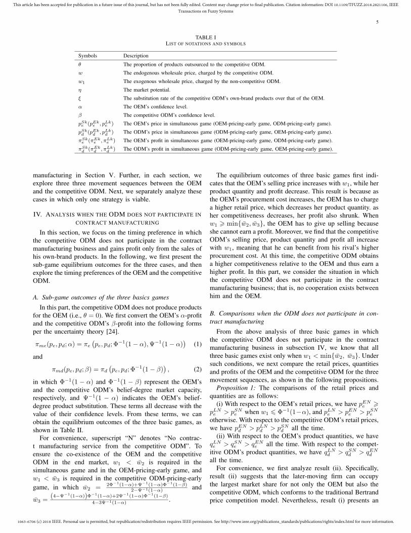
TABLE ILIST OF NOTATIONS AND SYMBOLS

Symbols Description

θ The proportion of products outsourced to the competitive ODM.

w The endogenous wholesale price, charged by the competitive ODM.

w1 The exogenous wholesale price, charged by the non-competitive ODM.

η The market potential.

ξ The substitution rate of the competitive ODM’s own-brand products over that of the OEM.

α The OEM’s confidence level.

β The competitive ODM’s confidence level.

pSke (pEk

e , pLke ) The OEM’s price in simultaneous game (OEM-pricing-early game, ODM-pricing-early game).

pSkd (pEk

d , pLkd ) The ODM’s price in simultaneous game (ODM-pricing-early game, OEM-pricing-early game).

πSke (πEk

e , πLke ) The OEM’s profit in simultaneous game (OEM-pricing-early game, ODM-pricing-early game).

πSkd (πEk

d , πLkd ) The ODM’s profit in simultaneous game (ODM-pricing-early game, OEM-pricing-early game).

manufacturing in Section V. Further, in each section, weexplore three three movement sequences between the OEMand the competitive ODM. Next, we separately analyze thesecases in which only one strategy is viable.

IV. ANALYSIS WHEN THE ODM DOES NOT PARTICIPATE INCONTRACT MANUFACTURING

In this section, we focus on the timing preference in whichthe competitive ODM does not participate in the contractmanufacturing business and gains profit only from the sales ofhis own-brand products. In the following, we first present thesub-game equilibrium outcomes for the three cases, and thenexplore the timing preferences of the OEM and the competitiveODM.

A. Sub-game outcomes of the three basics games

In this part, the competitive ODM does not produce productsfor the OEM (i.e., θ = 0). We first convert the OEM’s α-profitand the competitive ODM’s β-profit into the following formsper the uncertainty theory [24].

πme(pe, pd;α) = πe

(pe, pd; Φ

−1(1− α),Ψ−1(1− α))

(1)

and

πmd(pe, pd;β) = πd

(pe, pd; Φ

−1(1− β)), (2)

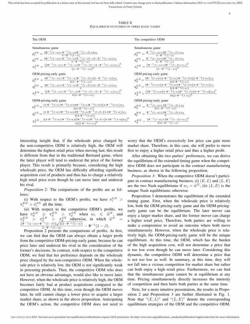
in which Φ−1(1 − α) and Φ−1(1 − β) represent the OEM’sand the competitive ODM’s belief-degree market capacity,respectively, and Ψ−1(1 − α) indicates the OEM’s belief-degree product substitution. These terms all decrease with thevalue of their confidence levels. From these terms, we canobtain the equilibrium outcomes of the three basic games, asshown in Table II.

For convenience, superscript “N” denotes “No contrac-t manufacturing service from the competitive ODM”. Toensure the co-existence of the OEM and the competitiveODM in the end market, w1 < w2 is required in thesimultaneous game and in the OEM-pricing-early game, andw1 < w3 is required in the competitive ODM-pricing-earlygame, in which w2 = 2Φ−1(1−α)+Ψ−1(1−α)Φ−1(1−β)

2−Ψ−1(1−α) and

w3 =(4−Ψ−1(1−α))Φ−1(1−α)+2Ψ−1(1−α)Φ−1(1−β)

4−3Ψ−1(1−α) .

The equilibrium outcomes of three basic games first indi-cates that the OEM’s selling price increases with w1, while herproduct quantity and profit decrease. This result is because asthe OEM’s procurement cost increases, the OEM has to chargea higher retail price, which decreases her product quantity. asher competitiveness decreases, her profit also shrunk. Whenw1 > min{w2, w3}, the OEM has to give up selling becauseshe cannot earn a profit. Moreover, we find that the competitiveODM’s selling price, product quantity and profit all increasewith w1, meaning that he can benefit from his rival’s higherprocurement cost. At this time, the competitive ODM obtainsa higher competitiveness relative to the OEM and thus earn ahigher profit. In this part, we consider the situation in whichthe competitive ODM does not participate in the contractmanufacturing business; that is, no cooperation exists betweenhim and the OEM.

B. Comparisons when the ODM does not participate in con-tract manufacturing

From the above analysis of three basic games in whichthe competitive ODM does not participate in the contractmanufacturing business in subsection IV, we know that allthree basic games exist only when w1 < min{w2, w3}. Undersuch conditions, we next compare the retail prices, quantitiesand profits of the OEM and the competitive ODM for the threemovement sequences, as shown in the following propositions.

Proposition 1: The comparisons of the retail prices andquantities are as follows:

(i) With respect to the OEM’s retail prices, we have pENe >

pLNe > pSN

e when w1 6 Φ−1(1−α), and pLNe > pEN

e > pSNe

otherwise. With respect to the competitive ODM’s retail prices,we have pEN

d > pLNd > pSN

d all the time.(ii) With respect to the OEM’s product quantities, we have

qLNe > qSN

e > qENe all the time. With respect to the compet-

itive ODM’s product quantities, we have qLNd > qSN

d > qENd

all the time.For convenience, we first analyze result (ii). Specifically,

result (ii) suggests that the later-moving firm can occupythe largest market share for not only the OEM but also thecompetitive ODM, which conforms to the traditional Bertrandprice competition model. Nevertheless, result (i) presents an



6

TABLE IIEQUILIBRIUM OUTCOMES OF THREE BASIC GAMES

The OEM The competitive ODM

Simultaneous game Simultaneous game

pSNe =

2Φ−1(1−α)+Ψ−1(1−α)Φ−1(1−β)+2w1

4−Ψ−1(1−α)pSNd =

Φ−1(1−α)+2Φ−1(1−β)+w1

4−Ψ−1(1−α)

qSNe =

2Φ−1(1−α)+Ψ−1(1−α)Φ−1(1−β)−(2−Ψ−1(1−α))w1

4−Ψ−1(1−α)qSNd =

Φ−1(1−α)+2Φ−1(1−β)+w1

4−Ψ−1(1−α)

πSNe =

(2Φ−1(1−α)+Ψ−1(1−α)Φ−1(1−β)−(2−Ψ−1(1−α))w1)2

(4−Ψ−1(1−α))2πSNe =

(Φ−1(1−α)+2Φ−1(1−β)+w1)2

(4−Ψ−1(1−α))2

OEM-pricing-early game OEM-pricing-early game

pENe =

2Φ−1(1−α)+Ψ−1(1−α)Φ−1(1−β)+(2−Ψ−1(1−α))w1

2(2−Ψ−1(1−α))pLNd =

2Φ−1(1−α)+(4−Ψ−1(1−α))Φ−1(1−β)+(2−Ψ−1(1−α))w1

4(2−Ψ−1(1−α))

qENe =

2Φ−1(1−α)+Ψ−1(1−α)Φ−1(1−β)+(2−Ψ−1(1−α))w14

qLNd =

2Φ−1(1−α)+(4−Ψ−1(1−α))Φ−1(1−β)+(2−Ψ−1(1−α))w1

4(2−Ψ−1(1−α))

πENe =

(2Φ−1(1−α)+Ψ−1(1−α)Φ−1(1−β)−(2−Ψ−1(1−α))w1)2

8(2−Ψ−1(1−α))πLNd =

(2Φ−1(1−α)+(4−Ψ−1(1−α))Φ−1(1−β)+(2−Ψ−1(1−α))w1)2

16(2−Ψ−1(1−α))2

ODM-pricing-early game ODM-pricing-early game

pLNe =

(4−Ψ−1(1−α))Φ−1(1−α)+2Ψ−1(1−α)Φ−1(1−β)+(4−Ψ−1(1−α))w1

4(2−Ψ−1(1−α))pENd =

Φ−1(1−α)+2Φ−1(1−β)+w1

2(2−Ψ−1(1−α))

qLNe =

(4−Ψ−1(1−α))Φ−1(1−α)+2Ψ−1(1−α)Φ−1(1−β)−(4−3Ψ−1(1−α))w1

4(2−Ψ−1(1−α))qENd =

Φ−1(1−α)+2Φ−1(1−β)+w14

.

πLNe =

((4−Ψ−1(1−α))Φ−1(1−α)+2Ψ−1(1−α)Φ−1(1−β)−(4−3Ψ−1(1−α))w1)2

16(2−Ψ−1(1−α))2πENd =

(Φ−1(1−α)+2Φ−1(1−β)+w1)2

8(2−Ψ−1(1−α)

interesting insight that, if the wholesale price charged bythe non-competitive ODM is relatively high, the OEM willdetermine the highest retail price when moving last; this resultis different from that in the traditional Bertrand game, wherethe latter player will tend to undercut the price of the formerplayer. This result is primarily because, considering the highwholesale price, the OEM has difficulty affording significantacquisition cost of products and thus has to charge a relativelyhigh retail price even though he can move later and undercuthis rival.

Proposition 2: The comparisons of the profits are as fol-lows:

(i) With respect to the OEM’s profits, we have πLNe >

πENe > πSN

e all the time.(ii) With respect to the competitive ODM’s profits, we

have πLNd > πEN

d > πSNd when w1 6 wN , and

πENd > πLN

d > πSNd otherwise, in which wN =

(Φ−1(1−α)+Φ−1(1−β))√

2(2−Ψ−1(1−α))

2−Ψ−1(1−α) − Φ−1(1− β).Proposition 2 presents the comparisons of profits. At first,

we can find that the OEM can always obtain a larger profitfrom the competitive ODM-pricing-early game, because he canprice later and undercut his rival in the consideration of theformer’s decisions. In contrast, with respect to the competitiveODM, we find that her preference depends on the wholesaleprice charged by the non-competitive ODM. When the whole-sale price is relatively low, the OEM is not significantly weakin procuring products. Then, the competitive ODM who doesnot have an obvious advantage, would also like to move later.However, when the wholesale price is relatively high, the OEMbecomes fairly bad at product acquisitions compared to thecompetitive ODM. At this time, even though the OEM moveslater, he still cannot charge a lower price to acquire a largermarket share, as shown in the above proposition. Anticipatingthe OEM’s action, the competitive ODM does not need to

worry that the OEM’s excessively low price can gain moremarket share. Therefore, in this case, she will prefer to movefirst to enjoy a higher retail price and thus a higher profit.

After obtaining the two parties’ preferences, we can derivethe equilibrium of the extended timing game when the compet-itive ODM does not participate in the contract manufacturingbusiness, as shown in the following proposition.

Proposition 3: When the competitive ODM doesn’t partici-pate in contract manufacturing business, (i) (E,L) and (L,E)are the two Nash equilibriums if w1 < wN , (ii) (L,E) is theunique Nash equilibriums otherwise.

Proposition 3 demonstrates the equilibrium of the extendedtiming game. First, when the wholesale price is relativelylow, both the OEM-pricing-early game and the ODM-pricing-early game can be the equilibrium. The later mover canenjoy a larger market share, and the former mover can chargea higher retail price. Therefore, both parties are willing tomake a compromise to avoid an outcome where both movesimultaneously. However, when the wholesale price is rela-tively high, the ODM-pricing-early game will be the uniqueequilibrium. At this time, the OEM, which has the burdenof the high acquisition cost, will not determine a price thatis too low even though he can move later. Considering thisdynamic, the competitive ODM will determine a price thatis not too low as well. In summary, at this time, they willnot fall into a vicious competition for market share but rathercan both enjoy a high retail price. Furthermore, we can findthat the simultaneous game cannot be at equilibrium at anytime. Pricing simultaneously directly increases the intensityof competition and then hurts both parties at the same time.

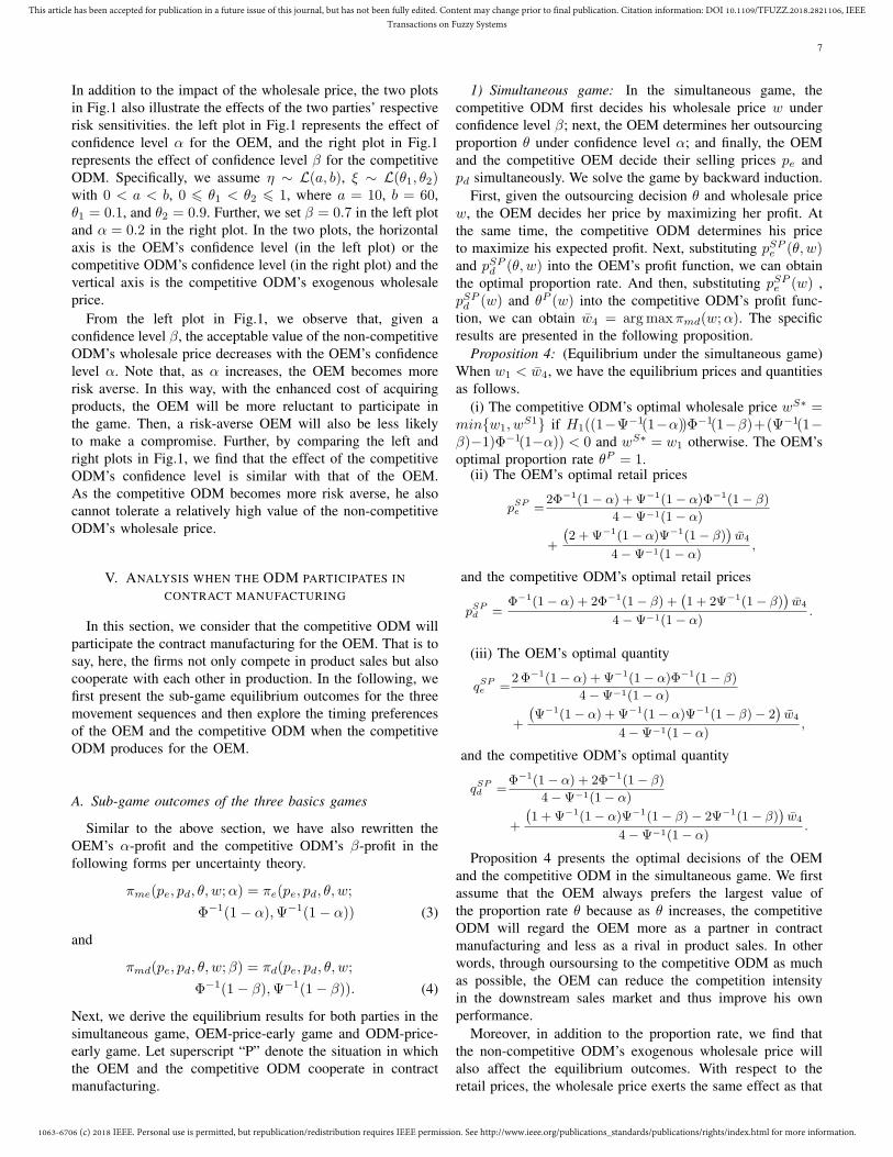
Next, for a more intuitive presentation, the results in Propo-sition 2 and Proposition 3 are further illustrated in Fig. 1.Note that “(E,L)” and “(L,E)” denote the correspondingequilibrium strategies of the OEM and the competitive ODM.



7

In addition to the impact of the wholesale price, the two plotsin Fig.1 also illustrate the effects of the two parties’ respectiverisk sensitivities. the left plot in Fig.1 represents the effect ofconfidence level α for the OEM, and the right plot in Fig.1represents the effect of confidence level β for the competitiveODM. Specifically, we assume η ∼ L(a, b), ξ ∼ L(θ1, θ2)with 0 < a < b, 0 6 θ1 < θ2 6 1, where a = 10, b = 60,θ1 = 0.1, and θ2 = 0.9. Further, we set β = 0.7 in the left plotand α = 0.2 in the right plot. In the two plots, the horizontalaxis is the OEM’s confidence level (in the left plot) or thecompetitive ODM’s confidence level (in the right plot) and thevertical axis is the competitive ODM’s exogenous wholesaleprice.

From the left plot in Fig.1, we observe that, given aconfidence level β, the acceptable value of the non-competitiveODM’s wholesale price decreases with the OEM’s confidencelevel α. Note that, as α increases, the OEM becomes morerisk averse. In this way, with the enhanced cost of acquiringproducts, the OEM will be more reluctant to participate inthe game. Then, a risk-averse OEM will also be less likelyto make a compromise. Further, by comparing the left andright plots in Fig.1, we find that the effect of the competitiveODM’s confidence level is similar with that of the OEM.As the competitive ODM becomes more risk averse, he alsocannot tolerate a relatively high value of the non-competitiveODM’s wholesale price.

V. ANALYSIS WHEN THE ODM PARTICIPATES INCONTRACT MANUFACTURING

In this section, we consider that the competitive ODM willparticipate the contract manufacturing for the OEM. That is tosay, here, the firms not only compete in product sales but alsocooperate with each other in production. In the following, wefirst present the sub-game equilibrium outcomes for the threemovement sequences and then explore the timing preferencesof the OEM and the competitive ODM when the competitiveODM produces for the OEM.

A. Sub-game outcomes of the three basics games

Similar to the above section, we have also rewritten theOEM’s α-profit and the competitive ODM’s β-profit in thefollowing forms per uncertainty theory.

πme(pe, pd, θ, w;α) = πe(pe, pd, θ, w;

Φ−1(1− α),Ψ−1(1− α)) (3)

and

πmd(pe, pd, θ, w;β) = πd(pe, pd, θ, w;

Φ−1(1− β),Ψ−1(1− β)). (4)

Next, we derive the equilibrium results for both parties in thesimultaneous game, OEM-price-early game and ODM-price-early game. Let superscript “P” denote the situation in whichthe OEM and the competitive ODM cooperate in contractmanufacturing.

1) Simultaneous game: In the simultaneous game, thecompetitive ODM first decides his wholesale price w underconfidence level β; next, the OEM determines her outsourcingproportion θ under confidence level α; and finally, the OEMand the competitive OEM decide their selling prices pe andpd simultaneously. We solve the game by backward induction.

First, given the outsourcing decision θ and wholesale pricew, the OEM decides her price by maximizing her profit. Atthe same time, the competitive ODM determines his priceto maximize his expected profit. Next, substituting pSP

e (θ, w)and pSP

d (θ, w) into the OEM’s profit function, we can obtainthe optimal proportion rate. And then, substituting pSP

e (w) ,pSPd (w) and θP (w) into the competitive ODM’s profit func-

tion, we can obtain w4 = argmaxπmd(w;α). The specificresults are presented in the following proposition.

Proposition 4: (Equilibrium under the simultaneous game)When w1 < w4, we have the equilibrium prices and quantitiesas follows.

(i) The competitive ODM’s optimal wholesale price wS∗ =min{w1, w

S1} if H1((1−Ψ−1(1−α))Φ−1(1−β)+(Ψ−1(1−β)−1)Φ−1(1−α)) < 0 and wS∗ = w1 otherwise. The OEM’soptimal proportion rate θP = 1.

(ii) The OEM’s optimal retail prices

pSPe =

2Φ−1(1− α) + Ψ−1(1− α)Φ−1(1− β)

4−Ψ−1(1− α)

+

(2 + Ψ−1(1− α)Ψ−1(1− β)

)w4

4−Ψ−1(1− α),

and the competitive ODM’s optimal retail prices

pSPd =

Φ−1(1− α) + 2Φ−1(1− β) +(1 + 2Ψ−1(1− β)

)w4

4−Ψ−1(1− α).

(iii) The OEM’s optimal quantity

qSPe =

2Φ−1(1− α) + Ψ−1(1− α)Φ−1(1− β)

4−Ψ−1(1− α)

+

(Ψ−1(1− α) + Ψ−1(1− α)Ψ−1(1− β)− 2

)w4

4−Ψ−1(1− α),

and the competitive ODM’s optimal quantity

qSPd =

Φ−1(1− α) + 2Φ−1(1− β)

4−Ψ−1(1− α)

+

(1 + Ψ−1(1− α)Ψ−1(1− β)− 2Ψ−1(1− β)

)w4

4−Ψ−1(1− α).

Proposition 4 presents the optimal decisions of the OEMand the competitive ODM in the simultaneous game. We firstassume that the OEM always prefers the largest value ofthe proportion rate θ because as θ increases, the competitiveODM will regard the OEM more as a partner in contractmanufacturing and less as a rival in product sales. In otherwords, through oursoursing to the competitive ODM as muchas possible, the OEM can reduce the competition intensityin the downstream sales market and thus improve his ownperformance.

Moreover, in addition to the proportion rate, we find thatthe non-competitive ODM’s exogenous wholesale price willalso affect the equilibrium outcomes. With respect to theretail prices, the wholesale price exerts the same effect as that



8

(E,L) or (L,E)

(L,E)

(E,L) or (L,E)

(L,E)

0 0.1 0.2 0.3 0.4 0.5 0.6 0.7 0.8 0.9 1

Confidence level α

0

20

40

60

80

100

120

140

Exo

geno

us w

hole

sale

pric

e w

1

(E,L) or (L,E)

(L,E)

0 0.1 0.2 0.3 0.4 0.5 0.6 0.7 0.8 0.9 1

Confidence level β

0

20

40

60

80

100

120

Exo

geno

us w

hole

sale

pric

e w

1

Fig. 1. Equilibrium pricing strategies

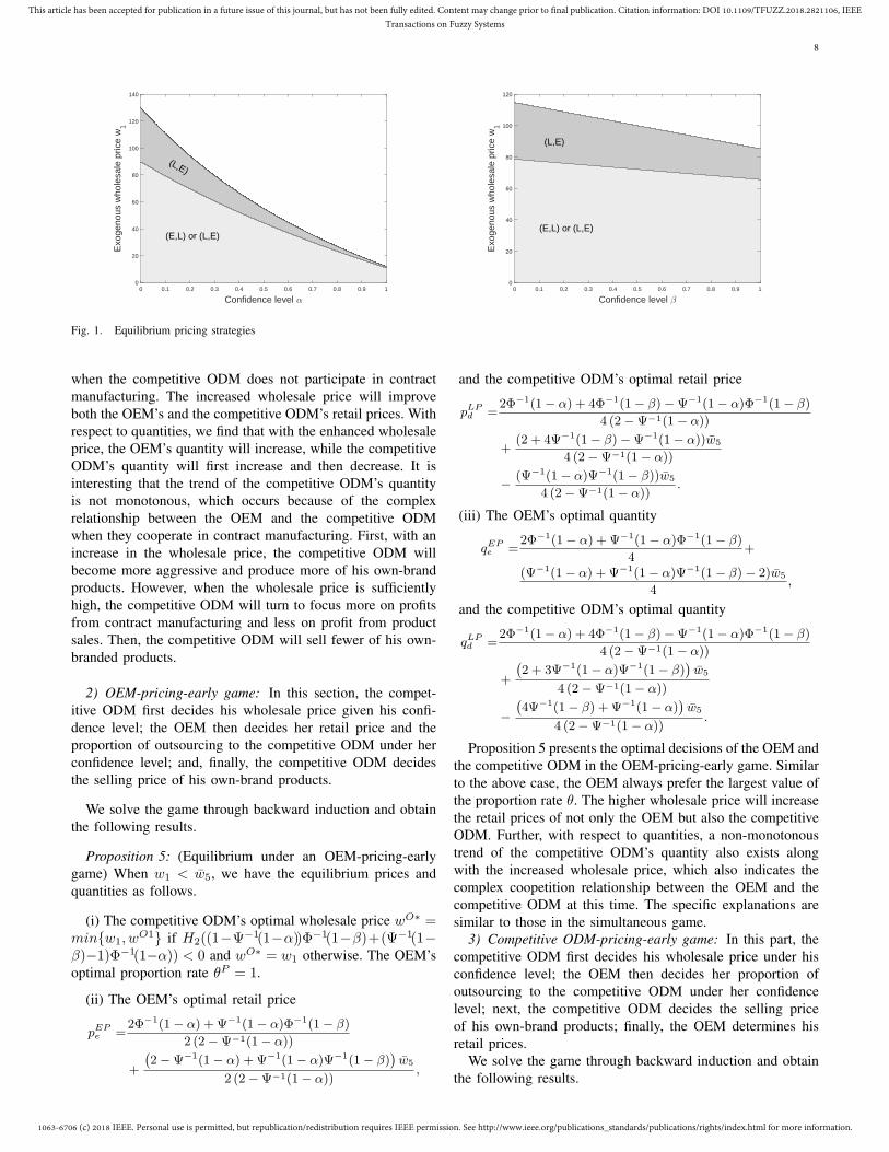
when the competitive ODM does not participate in contractmanufacturing. The increased wholesale price will improveboth the OEM’s and the competitive ODM’s retail prices. Withrespect to quantities, we find that with the enhanced wholesaleprice, the OEM’s quantity will increase, while the competitiveODM’s quantity will first increase and then decrease. It isinteresting that the trend of the competitive ODM’s quantityis not monotonous, which occurs because of the complexrelationship between the OEM and the competitive ODMwhen they cooperate in contract manufacturing. First, with anincrease in the wholesale price, the competitive ODM willbecome more aggressive and produce more of his own-brandproducts. However, when the wholesale price is sufficientlyhigh, the competitive ODM will turn to focus more on profitsfrom contract manufacturing and less on profit from productsales. Then, the competitive ODM will sell fewer of his own-branded products.

2) OEM-pricing-early game: In this section, the compet-itive ODM first decides his wholesale price given his confi-dence level; the OEM then decides her retail price and theproportion of outsourcing to the competitive ODM under herconfidence level; and, finally, the competitive ODM decidesthe selling price of his own-brand products.

We solve the game through backward induction and obtainthe following results.

Proposition 5: (Equilibrium under an OEM-pricing-earlygame) When w1 < w5, we have the equilibrium prices andquantities as follows.

(i) The competitive ODM’s optimal wholesale price wO∗ =min{w1, w

O1} if H2((1−Ψ−1(1−α))Φ−1(1−β)+(Ψ−1(1−β)−1)Φ−1(1−α)) < 0 and wO∗ = w1 otherwise. The OEM’soptimal proportion rate θP = 1.

(ii) The OEM’s optimal retail price

pEPe =

2Φ−1(1− α) + Ψ−1(1− α)Φ−1(1− β)

2 (2−Ψ−1(1− α))

+

(2−Ψ−1(1− α) + Ψ−1(1− α)Ψ−1(1− β)

)w5

2 (2−Ψ−1(1− α)),

and the competitive ODM’s optimal retail price

pLPd =

2Φ−1(1− α) + 4Φ−1(1− β)−Ψ−1(1− α)Φ−1(1− β)

4 (2−Ψ−1(1− α))

+(2 + 4Ψ−1(1− β)−Ψ−1(1− α))w5

4 (2−Ψ−1(1− α))

− (Ψ−1(1− α)Ψ−1(1− β))w5

4 (2−Ψ−1(1− α)).


qEPe =

2Φ−1(1− α) + Ψ−1(1− α)Φ−1(1− β)

4+

(Ψ−1(1− α) + Ψ−1(1− α)Ψ−1(1− β)− 2)w5

4,


qLPd =

2Φ−1(1− α) + 4Φ−1(1− β)−Ψ−1(1− α)Φ−1(1− β)

4 (2−Ψ−1(1− α))

+

(2 + 3Ψ−1(1− α)Ψ−1(1− β)

)w5

4 (2−Ψ−1(1− α))

−(4Ψ−1(1− β) + Ψ−1(1− α)

)w5

4 (2−Ψ−1(1− α)).

Proposition 5 presents the optimal decisions of the OEM andthe competitive ODM in the OEM-pricing-early game. Similarto the above case, the OEM always prefer the largest value ofthe proportion rate θ. The higher wholesale price will increasethe retail prices of not only the OEM but also the competitiveODM. Further, with respect to quantities, a non-monotonoustrend of the competitive ODM’s quantity also exists alongwith the increased wholesale price, which also indicates thecomplex coopetition relationship between the OEM and thecompetitive ODM at this time. The specific explanations aresimilar to those in the simultaneous game.

3) Competitive ODM-pricing-early game: In this part, thecompetitive ODM first decides his wholesale price under hisconfidence level; the OEM then decides her proportion ofoutsourcing to the competitive ODM under her confidencelevel; next, the competitive ODM decides the selling priceof his own-brand products; finally, the OEM determines hisretail prices.

We solve the game through backward induction and obtainthe following results.



9

Proposition 6: (Equilibrium under an ODM-pricing-earlygame) When w1 < w6, we have the equilibrium prices andquantities as follows.

(i) The competitive ODM’s optimal wholesale price wD∗ =min{w1, w

D1} if H3((1−Ψ−1(1−α))Φ−1(1−β)+(Ψ−1(1−β)−1)Φ−1(1−α)) < 0 and wD∗ = w1 otherwise. The OEM’soptimal proportion rate θP = 1.

(ii) The OEM’s optimal retail price

pLPe =

(4−Ψ−1(1− α))Φ−1(1− α) + 2Ψ−1(1− α)Φ−1(1− β)

4(2−Ψ−1(1− α))

+(4 + 2Ψ−1(1− α)Ψ−1(1− β))w6

4(2−Ψ−1(1− α))

− (Ψ−1(1− α) + (Ψ−1(1− α))2)w6

4(2−Ψ−1(1− α)),

and the competitive ODM’s optimal retail price

pEPd =

Φ−1(1− α) + 2Φ−1(1− β)

4− 2Ψ−1(1− α)+(

1−Ψ−1(1− α) + 2Ψ−1(1− β))w6

4− 2Ψ−1(1− α).


qLPe =

(4−Ψ−1(1− α))Φ−1(1− α) + 2Ψ−1(1− α)Φ−1(1− β)

4(2−Ψ−1(1− α))

− (4 + (Ψ−1(1− α))2)w6

4(2−Ψ−1(1− α))

− (3Ψ−1(1− α) + 2Ψ−1(1− α)Ψ−1(1− β))w6

4(2−Ψ−1(1− α)),


qEPd =

Φ−1(1− α) + 2Φ−1(1− β)

4

+(1 + Ψ−1(1− α)− 2Ψ−1(1− β))w6

4.

Proposition 6 presents the optimal decisions of the OEMand the competitive ODM in the ODM-pricing-early game.The effects and trends are also similar as those in the abovetwo cases. These results indicate that the selection of dif-ferent movement sequences will not affect the coopetitionrelationship between the OEM and the competitive ODMquantitatively. These cases under three different movementsequences differ only in the intensities of the competitioneffect and the cooperation effect. The three cases all existonly when the non-competitive ODM’s wholesale price is notexcessively high. Specific comparisons of the retail prices,quantities and profits of the OEM and the competitive OEMare presented in the following subsection.

B. Comparisons when the ODM participates in contract man-ufacturing

From the above analysis of three basic games when theODM participates in contract manufacturing, we know that allthree basic games exit only when w1 < min{w4, w6}, inwhich w1 < w4 is needed to maintain the existence of boththe simultaneous game and the OEM-pricing-early game andw1 < w6 is needed to maintain the existence of the ODM-pricing-early game. We then respectively compare the retail

prices, quantities and profits of the OEM and the competitiveODM.

1) Comparisons of the OEM: In this part, we compare theretail prices, quantities and profits of the OEM. The followingproposition presents the comparisons of the retail price.

Proposition 7: The comparison of the retail price of theOEM is as follows:

(i) When (1−Ψ−1(1−α))Φ−1(1−β)+(Ψ−1(1−β)−1)Φ−1(1−α)<0, pEP

e >pLPe >pSP

e if w16wa, and pEPe >pSP

e >pLPe

otherwise. Here wa = Φ−1(1−α)+2Φ−1(1−β)3−Ψ−1(1−α)−2Ψ−1(1−β) .

(ii) When (1−Ψ−1(1−α))Φ−1(1−β)+(Ψ−1(1−β)−1)Φ−1(1−α)> 0, pEP

e > pLPe > pSP

e if w1 6 Φ−1(1−α)1−Ψ−1(1−α) , and pLP

e >

pEPe >pSP

e otherwise.Proposition 7 shows the comparison of the OEM’s retail

prices under the simultaneous game, the OEM-pricing-earlygame and the competitive ODM-pricing-early game. We findthat the OEM’s pricing strategy depends on the combinedeffects of the threshold value (1−Ψ−1(1−α))Ψ−1(1−β)+(Ψ−1(1 − β) − 1)Ψ−1(1 − α), determined by the risk levelsof two parties, and the non-competitive ODM’s wholesaleprice w1. We apply the numerical analysis here to study themanagemental meaning of the condition (1−Ψ−1(1−α))Φ−1(1−β)+(Ψ−1(1−β)−1)Φ−1(1−α) because of its not intuitive form.We find (1−Ψ−1(1−α))Φ−1(1−β)+(Ψ−1(1−β)−1)Φ−1(1−α)<0when the OEM is relatively risk loving and (1−Ψ−1(1−α))Φ−1(1−β)+(Ψ−1(1−β)−1)Φ−1(1−α)>0 when the OEM isrelatively risk averse. Compared to the results in Proposition 1,we find that the comparisons of a relatively risk averse OEM’sretail prices keep the same no matter whether the competitiveOEM participates in the contract manufacturing business, asshown in the result (ii). Nevertheless, result (i) indicates that,when the OEM becomes sufficiently risk-loving, the last-moving OEM’s retail price pLP

e becomes the smallest oneinstead of the largest one even though wholesale price isrelatively high. That is resulted from the competitive ODM’sreaction at this time. The high wholesale price endows thecompetitive ODM with a large space to enhance her wholesaleprice and then her profit from manufacturing business, whichboth alleviating the ODM’s aggressive attitude. Therefore, inthe case of such a less aggressive ODM, the OEM still preferto move later to enjoy the second-mover advantage.

Next, we compare the quantities of the OEM under differentmovement sequences.

Proposition 8: The comparison of the quantity of the OEMis as follows:

(i) When (1−Ψ−1(1−α))Φ−1(1−β)+(Ψ−1(1−β)−1)Φ−1(1−α) < 0, we have qLP

e > qSPe > qEP

e if w1 6 wa, qSPe >

qLPe > qEP

e if wa < w1 <Φ−1(1−α)+Ψ−1(1−α)Φ−1(1−β)

1−Ψ−1(1−α)Ψ−1(1−β) , andqSPe >qEP

e >qLPe otherwise.

(ii) When (1−Ψ−1(1−α))Φ−1(1−β)+(Ψ−1(1−β)−1)Φ−1(1−α)>0, we have qLP

e >qSPe >qEP

e all the time.Proposition 8 presents the comparisons of the OEM’s

quantities when the competitive ODM participates in thecontract manufacturing business. Compared to the results inProposition 10, we find that the comparisons of a relativelyrisk averse OEM’s retail quantities also remain the sameregardless of whether the competitive OEM participates in



10

the contract manufacturing business. Nevertheless, when theOEM becomes sufficiently risk loving, the comparisons ofthe OEM’s quantities are divided into three cases. When thewholesale price for the non-competitive ODM is fairly small,qLPe > qSP

e > qEPe remains. However, with an increasing

wholesale price, the comparison becomes qSPe >qLP

e >qEPe .

Further, when the wholesale price becomes sufficiently high,the comparison result becomes qSP

e >qEPe >qLP

e . In summary,qLPe decreases with the wholesale price, which means that

the OEM is less likely to enjoy the second-mover advantage.This result is primarily because as his product acquisition costincreases, the OEM is less willing to move later to price lowand sell more.

After deriving the comparisons of the retail prices andquantities, we next compare the profits of the OEM underdifferent movement sequences.

Proposition 9: The following relationships concerning theequilibrium profit of the OEM hold in three basic games:

(i) When (1−Ψ−1(1−α))Φ−1(1−β)+(Ψ−1(1−β)−1)Φ−1(1−α) < 0, we have (a) πLP

e > πEPe > πSP

e if w1 < we4; (b)πEPe >πLP

e >πSPe if we46w1<we1; (c) πEP

e >πSPe >πLP

e

if we16w1<wD.(ii) When (1−Ψ−1(1−α))Φ−1(1−β)+(Ψ−1(1−β)−1)Φ−1(1−

α)>0, we have πLPe >πEP

e >πSPe all the time.

Proposition 9 presents the comparisons of the OEM’s profitswhen the competitive ODM participates in the contract man-ufacturing business. In contrast to results in Proposition 2,we find that the comparisons of the risk averse OEM’s profitstill remain the same even though the competitive ODMproduces products for the OEM. However, in the case of asufficiently risk-loving OEM, the comparisons are divided intothree situations. When the non-competitive ODM’s wholesaleprice is fairly small, πLP

e >πEPe >πSP

e maintains. However,with increases in the wholesale price, the comparison becomesπEPe > πLP

e > πSPe . Further, when the wholesale price

becomes sufficiently high, the comparison result becomesπEPe >πSP

e >πLPe . The change trend of πLP

e is similar to thatof qLP

e . That is to say, the increased wholesale price limitsthe OEM’s ability to reduce the retail price and occupy moremarket share when she moves later. Hence, even though shemoves later, the OEM still cannot undercut the former mover’sprice. In this way, she loses the second-mover advantage hereand achieves a lower profit.

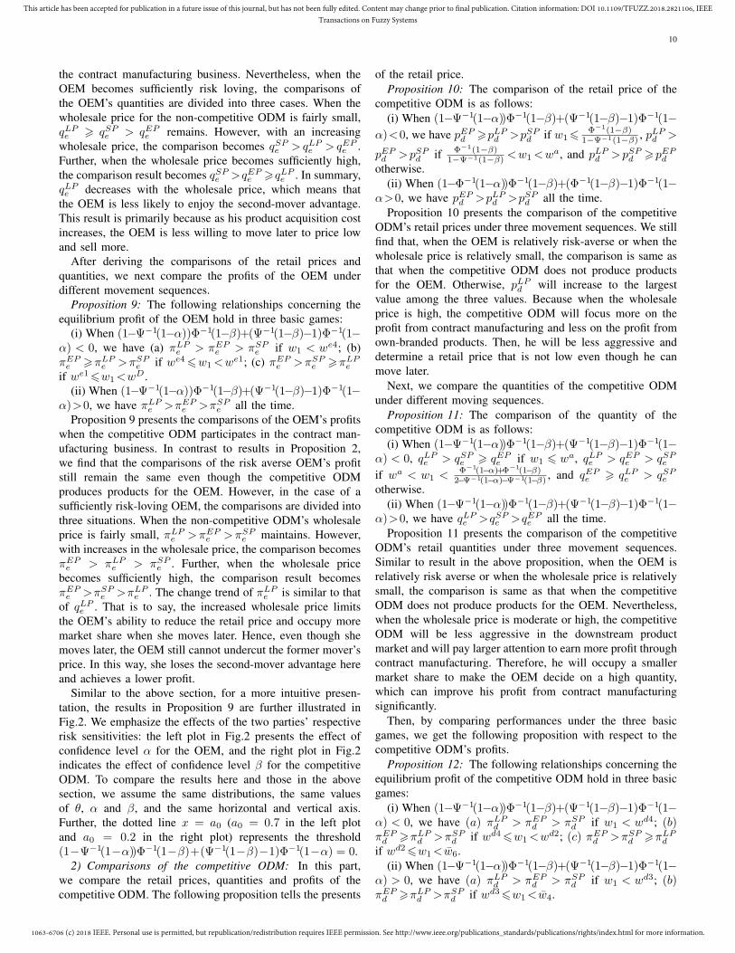
Similar to the above section, for a more intuitive presen-tation, the results in Proposition 9 are further illustrated inFig.2. We emphasize the effects of the two parties’ respectiverisk sensitivities: the left plot in Fig.2 presents the effect ofconfidence level α for the OEM, and the right plot in Fig.2indicates the effect of confidence level β for the competitiveODM. To compare the results here and those in the abovesection, we assume the same distributions, the same valuesof θ, α and β, and the same horizontal and vertical axis.Further, the dotted line x = a0 (a0 = 0.7 in the left plotand a0 = 0.2 in the right plot) represents the threshold(1−Ψ−1(1−α))Φ−1(1−β)+(Ψ−1(1−β)−1)Φ−1(1−α) = 0.

2) Comparisons of the competitive ODM: In this part,we compare the retail prices, quantities and profits of thecompetitive ODM. The following proposition tells the presents

of the retail price.Proposition 10: The comparison of the retail price of the

competitive ODM is as follows:(i) When (1−Ψ−1(1−α))Φ−1(1−β)+(Ψ−1(1−β)−1)Φ−1(1−

α)<0, we have pEPd >pLP

d >pSPd if w16 Φ−1(1−β)

1−Ψ−1(1−β) , pLPd >

pEPd >pSP

d if Φ−1(1−β)1−Ψ−1(1−β) <w1<wa, and pLP

d >pSPd >pEP

d

otherwise.(ii) When (1−Φ−1(1−α))Φ−1(1−β)+(Φ−1(1−β)−1)Φ−1(1−

α>0, we have pEPd >pLP

d >pSPd all the time.

Proposition 10 presents the comparison of the competitiveODM’s retail prices under three movement sequences. We stillfind that, when the OEM is relatively risk-averse or when thewholesale price is relatively small, the comparison is same asthat when the competitive ODM does not produce productsfor the OEM. Otherwise, pLP

d will increase to the largestvalue among the three values. Because when the wholesaleprice is high, the competitive ODM will focus more on theprofit from contract manufacturing and less on the profit fromown-branded products. Then, he will be less aggressive anddetermine a retail price that is not low even though he canmove later.

Next, we compare the quantities of the competitive ODMunder different moving sequences.

Proposition 11: The comparison of the quantity of thecompetitive ODM is as follows:

(i) When (1−Ψ−1(1−α))Φ−1(1−β)+(Ψ−1(1−β)−1)Φ−1(1−α) < 0, qLP

e > qSPe > qEP

e if w1 6 wa, qLPe > qEP

e > qSPe

if wa < w1 < Φ−1(1−α)+Φ−1(1−β)2−Ψ−1(1−α)−Ψ−1(1−β) , and qEP

e > qLPe > qSP

e

otherwise.(ii) When (1−Ψ−1(1−α))Φ−1(1−β)+(Ψ−1(1−β)−1)Φ−1(1−

α)>0, we have qLPe >qSP

e >qEPe all the time.

Proposition 11 presents the comparison of the competitiveODM’s retail quantities under three movement sequences.Similar to result in the above proposition, when the OEM isrelatively risk averse or when the wholesale price is relativelysmall, the comparison is same as that when the competitiveODM does not produce products for the OEM. Nevertheless,when the wholesale price is moderate or high, the competitiveODM will be less aggressive in the downstream productmarket and will pay larger attention to earn more profit throughcontract manufacturing. Therefore, he will occupy a smallermarket share to make the OEM decide on a high quantity,which can improve his profit from contract manufacturingsignificantly.

Then, by comparing performances under the three basicgames, we get the following proposition with respect to thecompetitive ODM’s profits.

Proposition 12: The following relationships concerning theequilibrium profit of the competitive ODM hold in three basicgames:

(i) When (1−Ψ−1(1−α))Φ−1(1−β)+(Ψ−1(1−β)−1)Φ−1(1−α) < 0, we have (a) πLP

d > πEPd > πSP

d if w1 < wd4; (b)πEPd >πLP

d >πSPd if wd46w1<wd2; (c) πEP

d >πSPd >πLP

d

if wd26w1<w6.(ii) When (1−Ψ−1(1−α))Φ−1(1−β)+(Ψ−1(1−β)−1)Φ−1(1−

α) > 0, we have (a) πLPd > πEP

d > πSPd if w1 < wd3; (b)

πEPd >πLP

d >πSPd if wd36w1<w4.



11

L>E>S

E>L>S

E>S>L

a00 0.1 0.2 0.3 0.4 0.5 0.6 0.7 0.8 0.9 1

Confidence level α

0

20

40

60

80

100

120

140

160

Exo

geno

us w

hole

sale

pric

e w

1

L>E>SE>L>S

E>S>L

a00 0.1 0.2 0.3 0.4 0.5 0.6 0.7 0.8 0.9 1

Confidence level β

0

50

100

150

200

250

Exo

geno

us w

hole

sale

pric

e w

1

Fig. 2. Preferred pricing strategies of the OEM

L>E>S

E>L>S

E>S>L

E>L>S

a00 0.1 0.2 0.3 0.4 0.5 0.6 0.7 0.8 0.9 1

Confidence level α

0

20

40

60

80

100

120

140

160

Exo

geno

us w

hole

sale

pric

e w

1

L>E>SE>L>S

E>S>L

E>L>S

a00 0.1 0.2 0.3 0.4 0.5 0.6 0.7 0.8 0.9 1

Confidence level β

0

50

100

150

200

250

Exo

geno

us w

hole

sale

pric

e w

1

Fig. 3. Preferred pricing strategies of the competitive ODM

Proposition 12 presents the competitive ODM’s preferencesin the simultaneous game, the OEM-pricing-early game andthe CCM-pricing-early game. Similar to Proposition 9, we alsofind that the CCM’s pricing strategy depends on the combinedeffects of the threshold value (1−Ψ−1(1−α))Φ−1(1−β)+(Ψ−1(1−β)−1)Φ−1(1−α) and the non-competitive ODM’swholesale price w1. Through this comparison, we find thatwith increases in the wholesale price, the πLP

d always becomeslower in comparison and that when the competitive ODM isrelatively risk loving, this trend is more remarkable. This resultis because the high wholesale price increases the competitiveODM’s profit from contract manufacturing. A more risk-lovingODM will focus more on earning profit from this part, andwill not prefer to move later. In contrast to the result inProposition 2, we can find that at this time, the competitiveODM will consider the OEM less as a competitor and moreas a cooperator. Therefore, the competitive ODM would liketo give up the second-mover advantage in the downstreamproduct sales market.

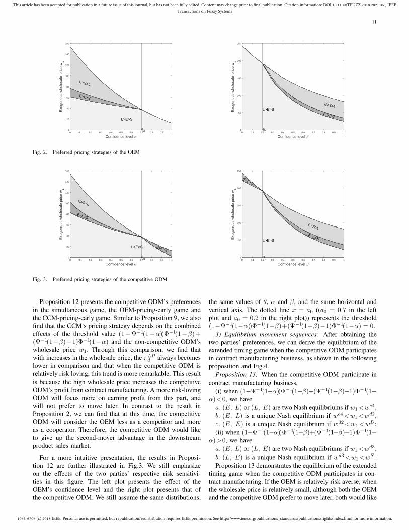
For a more intuitive presentation, the results in Proposi-tion 12 are further illustrated in Fig.3. We still emphasizeon the effects of the two parties’ respective risk sensitivi-ties in this figure. The left plot presents the effect of theOEM’s confidence level and the right plot presents that ofthe competitive ODM. We still assume the same distributions,

the same values of θ, α and β, and the same horizontal andvertical axis. The dotted line x = a0 ((a0 = 0.7 in the leftplot and a0 = 0.2 in the right plot)) represents the threshold(1−Ψ−1(1−α))Φ−1(1−β)+(Ψ−1(1−β)−1)Φ−1(1−α) = 0.

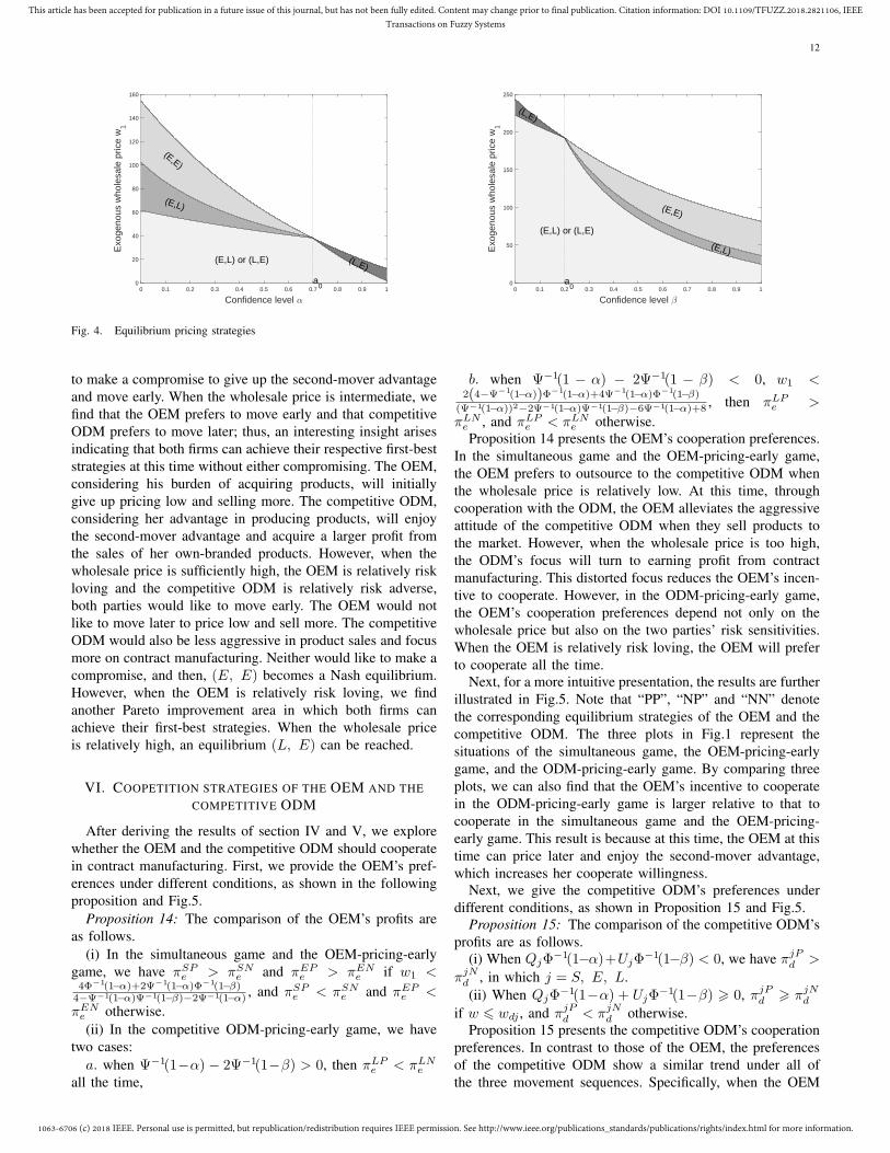
3) Equilibrium movement sequences: After obtaining thetwo parties’ preferences, we can derive the equilibrium of theextended timing game when the competitive ODM participatesin contract manufacturing business, as shown in the followingproposition and Fig.4.

Proposition 13: When the competitive ODM participate incontract manufacturing business,

(i) when (1−Ψ−1(1−α))Φ−1(1−β)+(Ψ−1(1−β)−1)Φ−1(1−α)<0, we have

a. (E, L) or (L, E) are two Nash equilibriums if w1<we4,b. (E, L) is a unique Nash equilibrium if we4<w1<wd2,c. (E, E) is a unique Nash equilibrium if wd2<w1<wD;(ii) when (1−Ψ−1(1−α))Φ−1(1−β)+(Ψ−1(1−β)−1)Φ−1(1−

α)>0, we havea. (E, L) or (L, E) are two Nash equilibriums if w1<wd3,b. (L, E) is a unique Nash equilibrium if wd3<w1<wS .Proposition 13 demonstrates the equilibrium of the extended

timing game when the competitive ODM participates in con-tract manufacturing. If the OEM is relatively risk averse, whenthe wholesale price is relatively small, although both the OEMand the competitive ODM prefer to move later, both would like



12

a0

(E,L) or (L,E)

(E,L)

(E,E)

(L,E)

0 0.1 0.2 0.3 0.4 0.5 0.6 0.7 0.8 0.9 1

Confidence level α

0

20

40

60

80

100

120

140

160

Exo

geno

us w

hole

sale

pric

e w

1

a0

(E,L) or (L,E)

(E,L)

(E,E)

(L,E)

0 0.1 0.2 0.3 0.4 0.5 0.6 0.7 0.8 0.9 1

Confidence level β

0

50

100

150

200

250

Exo

geno

us w

hole

sale

pric

e w

1

Fig. 4. Equilibrium pricing strategies

to make a compromise to give up the second-mover advantageand move early. When the wholesale price is intermediate, wefind that the OEM prefers to move early and that competitiveODM prefers to move later; thus, an interesting insight arisesindicating that both firms can achieve their respective first-beststrategies at this time without either compromising. The OEM,considering his burden of acquiring products, will initiallygive up pricing low and selling more. The competitive ODM,considering her advantage in producing products, will enjoythe second-mover advantage and acquire a larger profit fromthe sales of her own-branded products. However, when thewholesale price is sufficiently high, the OEM is relatively riskloving and the competitive ODM is relatively risk adverse,both parties would like to move early. The OEM would notlike to move later to price low and sell more. The competitiveODM would also be less aggressive in product sales and focusmore on contract manufacturing. Neither would like to make acompromise, and then, (E, E) becomes a Nash equilibrium.However, when the OEM is relatively risk loving, we findanother Pareto improvement area in which both firms canachieve their first-best strategies. When the wholesale priceis relatively high, an equilibrium (L, E) can be reached.

VI. COOPETITION STRATEGIES OF THE OEM AND THECOMPETITIVE ODM

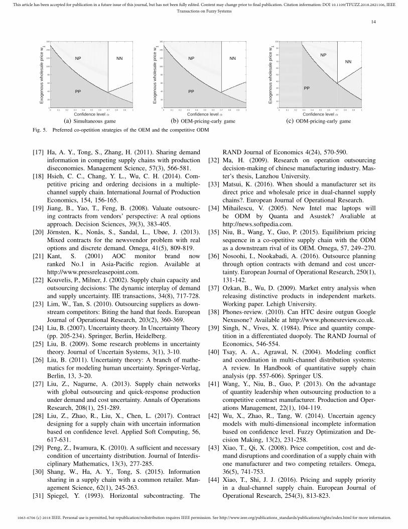
After deriving the results of section IV and V, we explorewhether the OEM and the competitive ODM should cooperatein contract manufacturing. First, we provide the OEM’s pref-erences under different conditions, as shown in the followingproposition and Fig.5.

Proposition 14: The comparison of the OEM’s profits areas follows.

(i) In the simultaneous game and the OEM-pricing-earlygame, we have πSP

e > πSNe and πEP

e > πENe if w1 <

4Φ−1(1−α)+2Ψ−1(1−α)Φ−1(1−β)4−Ψ−1(1−α)Ψ−1(1−β)−2Ψ−1(1−α) , and πSP

e < πSNe and πEP

e <

πENe otherwise.(ii) In the competitive ODM-pricing-early game, we have

two cases:a. when Ψ−1(1−α) − 2Ψ−1(1−β) > 0, then πLP

e < πLNe

all the time,

b. when Ψ−1(1 − α) − 2Ψ−1(1 − β) < 0, w1 <2(4−Ψ−1(1−α))Φ−1(1−α)+4Ψ−1(1−α)Φ−1(1−β)

(Ψ−1(1−α))2−2Ψ−1(1−α)Ψ−1(1−β)−6Ψ−1(1−α)+8 , then πLPe >

πLNe , and πLP

e < πLNe otherwise.

Proposition 14 presents the OEM’s cooperation preferences.In the simultaneous game and the OEM-pricing-early game,the OEM prefers to outsource to the competitive ODM whenthe wholesale price is relatively low. At this time, throughcooperation with the ODM, the OEM alleviates the aggressiveattitude of the competitive ODM when they sell products tothe market. However, when the wholesale price is too high,the ODM’s focus will turn to earning profit from contractmanufacturing. This distorted focus reduces the OEM’s incen-tive to cooperate. However, in the ODM-pricing-early game,the OEM’s cooperation preferences depend not only on thewholesale price but also on the two parties’ risk sensitivities.When the OEM is relatively risk loving, the OEM will preferto cooperate all the time.

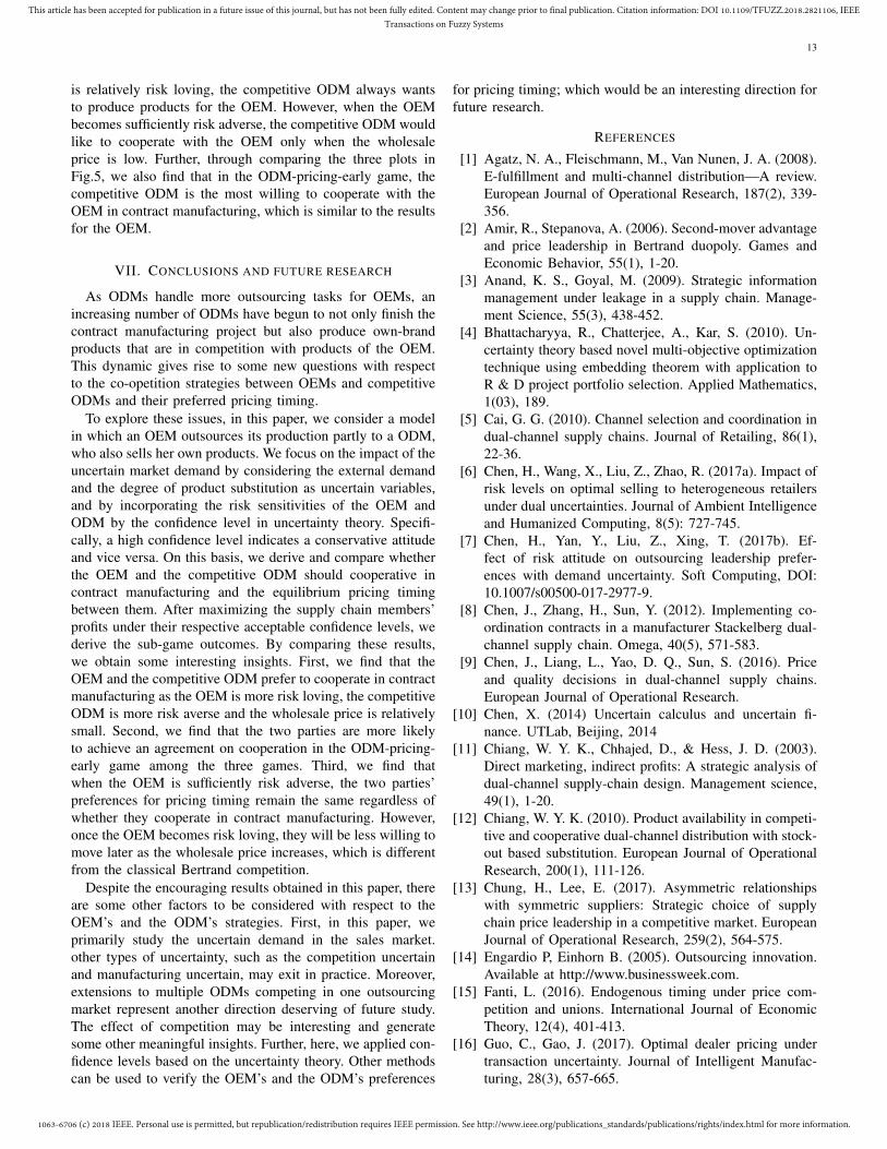
Next, for a more intuitive presentation, the results are furtherillustrated in Fig.5. Note that “PP”, “NP” and “NN” denotethe corresponding equilibrium strategies of the OEM and thecompetitive ODM. The three plots in Fig.1 represent thesituations of the simultaneous game, the OEM-pricing-earlygame, and the ODM-pricing-early game. By comparing threeplots, we can also find that the OEM’s incentive to cooperatein the ODM-pricing-early game is larger relative to that tocooperate in the simultaneous game and the OEM-pricing-early game. This result is because at this time, the OEM at thistime can price later and enjoy the second-mover advantage,which increases her cooperate willingness.

Next, we give the competitive ODM’s preferences underdifferent conditions, as shown in Proposition 15 and Fig.5.

Proposition 15: The comparison of the competitive ODM’sprofits are as follows.

(i) When QjΦ−1(1−α)+UjΦ

−1(1−β) < 0, we have πjPd >

πjNd , in which j = S, E, L.(ii) When QjΦ

−1(1−α) + UjΦ−1(1−β) > 0, πjP

d > πjNd

if w 6 wdj , and πjPd < πjN

d otherwise.Proposition 15 presents the competitive ODM’s cooperation

preferences. In contrast to those of the OEM, the preferencesof the competitive ODM show a similar trend under all ofthe three movement sequences. Specifically, when the OEM



13

is relatively risk loving, the competitive ODM always wantsto produce products for the OEM. However, when the OEMbecomes sufficiently risk adverse, the competitive ODM wouldlike to cooperate with the OEM only when the wholesaleprice is low. Further, through comparing the three plots inFig.5, we also find that in the ODM-pricing-early game, thecompetitive ODM is the most willing to cooperate with theOEM in contract manufacturing, which is similar to the resultsfor the OEM.

VII. CONCLUSIONS AND FUTURE RESEARCH

As ODMs handle more outsourcing tasks for OEMs, anincreasing number of ODMs have begun to not only finish thecontract manufacturing project but also produce own-brandproducts that are in competition with products of the OEM.This dynamic gives rise to some new questions with respectto the co-opetition strategies between OEMs and competitiveODMs and their preferred pricing timing.

To explore these issues, in this paper, we consider a modelin which an OEM outsources its production partly to a ODM,who also sells her own products. We focus on the impact of theuncertain market demand by considering the external demandand the degree of product substitution as uncertain variables,and by incorporating the risk sensitivities of the OEM andODM by the confidence level in uncertainty theory. Specifi-cally, a high confidence level indicates a conservative attitudeand vice versa. On this basis, we derive and compare whetherthe OEM and the competitive ODM should cooperative incontract manufacturing and the equilibrium pricing timingbetween them. After maximizing the supply chain members’profits under their respective acceptable confidence levels, wederive the sub-game outcomes. By comparing these results,we obtain some interesting insights. First, we find that theOEM and the competitive ODM prefer to cooperate in contractmanufacturing as the OEM is more risk loving, the competitiveODM is more risk averse and the wholesale price is relativelysmall. Second, we find that the two parties are more likelyto achieve an agreement on cooperation in the ODM-pricing-early game among the three games. Third, we find thatwhen the OEM is sufficiently risk adverse, the two parties’preferences for pricing timing remain the same regardless ofwhether they cooperate in contract manufacturing. However,once the OEM becomes risk loving, they will be less willing tomove later as the wholesale price increases, which is differentfrom the classical Bertrand competition.

Despite the encouraging results obtained in this paper, thereare some other factors to be considered with respect to theOEM’s and the ODM’s strategies. First, in this paper, weprimarily study the uncertain demand in the sales market.other types of uncertainty, such as the competition uncertainand manufacturing uncertain, may exit in practice. Moreover,extensions to multiple ODMs competing in one outsourcingmarket represent another direction deserving of future study.The effect of competition may be interesting and generatesome other meaningful insights. Further, here, we applied con-fidence levels based on the uncertainty theory. Other methodscan be used to verify the OEM’s and the ODM’s preferences

for pricing timing; which would be an interesting direction forfuture research.

REFERENCES

[1] Agatz, N. A., Fleischmann, M., Van Nunen, J. A. (2008).E-fulfillment and multi-channel distribution—A review.European Journal of Operational Research, 187(2), 339-356.

[2] Amir, R., Stepanova, A. (2006). Second-mover advantageand price leadership in Bertrand duopoly. Games andEconomic Behavior, 55(1), 1-20.

[3] Anand, K. S., Goyal, M. (2009). Strategic informationmanagement under leakage in a supply chain. Manage-ment Science, 55(3), 438-452.

[4] Bhattacharyya, R., Chatterjee, A., Kar, S. (2010). Un-certainty theory based novel multi-objective optimizationtechnique using embedding theorem with application toR & D project portfolio selection. Applied Mathematics,1(03), 189.

[5] Cai, G. G. (2010). Channel selection and coordination indual-channel supply chains. Journal of Retailing, 86(1),22-36.

[6] Chen, H., Wang, X., Liu, Z., Zhao, R. (2017a). Impact ofrisk levels on optimal selling to heterogeneous retailersunder dual uncertainties. Journal of Ambient Intelligenceand Humanized Computing, 8(5): 727-745.

[7] Chen, H., Yan, Y., Liu, Z., Xing, T. (2017b). Ef-fect of risk attitude on outsourcing leadership prefer-ences with demand uncertainty. Soft Computing, DOI:10.1007/s00500-017-2977-9.

[8] Chen, J., Zhang, H., Sun, Y. (2012). Implementing co-ordination contracts in a manufacturer Stackelberg dual-channel supply chain. Omega, 40(5), 571-583.

[9] Chen, J., Liang, L., Yao, D. Q., Sun, S. (2016). Priceand quality decisions in dual-channel supply chains.European Journal of Operational Research.

[10] Chen, X. (2014) Uncertain calculus and uncertain fi-nance. UTLab, Beijing, 2014

[11] Chiang, W. Y. K., Chhajed, D., & Hess, J. D. (2003).Direct marketing, indirect profits: A strategic analysis ofdual-channel supply-chain design. Management science,49(1), 1-20.

[12] Chiang, W. Y. K. (2010). Product availability in competi-tive and cooperative dual-channel distribution with stock-out based substitution. European Journal of OperationalResearch, 200(1), 111-126.

[13] Chung, H., Lee, E. (2017). Asymmetric relationshipswith symmetric suppliers: Strategic choice of supplychain price leadership in a competitive market. EuropeanJournal of Operational Research, 259(2), 564-575.

[14] Engardio P, Einhorn B. (2005). Outsourcing innovation.Available at http://www.businessweek.com.

[15] Fanti, L. (2016). Endogenous timing under price com-petition and unions. International Journal of EconomicTheory, 12(4), 401-413.

[16] Guo, C., Gao, J. (2017). Optimal dealer pricing undertransaction uncertainty. Journal of Intelligent Manufac-turing, 28(3), 657-665.



14

PP

NP NN

0 0.1 0.2 0.3 0.4 0.5 0.6 0.7 0.8 0.9 1

Confidence level α

0

20

40

60

80

100

120

140

160E

xoge

nous

who

lesa

le p

rice

w1

(a) Simultaneous game

PP

NP NN

0 0.1 0.2 0.3 0.4 0.5 0.6 0.7 0.8 0.9 1

Confidence level α

0

20

40

60

80

100

120

140

160

Exo

geno

us w

hole

sale

pric

e w

1

(b) OEM-pricing-early game

PP

NP

NN

0 0.1 0.2 0.3 0.4 0.5 0.6 0.7 0.8 0.9 1

Confidence level α

0

10

20

30

40

50

60

70

80

90

100

Exo

geno

us w

hole

sale

pric

e w

1

(c) ODM-pricing-early game

Fig. 5. Preferred co-opetition strategies of the OEM and the competitive ODM

[17] Ha, A. Y., Tong, S., Zhang, H. (2011). Sharing demandinformation in competing supply chains with productiondiseconomies. Management Science, 57(3), 566-581.

[18] Hsieh, C. C., Chang, Y. L., Wu, C. H. (2014). Com-petitive pricing and ordering decisions in a multiple-channel supply chain. International Journal of ProductionEconomics, 154, 156-165.

[19] Jiang, B., Yao, T., Feng, B. (2008). Valuate outsourc-ing contracts from vendors’ perspective: A real optionsapproach. Decision Sciences, 39(3), 383-405.

[20] Jornsten, K., Nonas, S., Sandal, L., Ubøe, J. (2013).Mixed contracts for the newsvendor problem with realoptions and discrete demand. Omega, 41(5), 809-819.

[21] Kant, S. (2001) AOC monitor brand nowranked No.1 in Asia-Pacific region. Available athttp://www.pressreleasepoint.com.

[22] Kouvelis, P., Milner, J. (2002). Supply chain capacity andoutsourcing decisions: The dynamic interplay of demandand supply uncertainty. IIE transactions, 34(8), 717-728.

[23] Lim, W., Tan, S. (2010). Outsourcing suppliers as down-stream competitors: Biting the hand that feeds. EuropeanJournal of Operational Research, 203(2), 360-369.

[24] Liu, B. (2007). Uncertainty theory. In Uncertainty Theory(pp. 205-234). Springer, Berlin, Heidelberg.

[25] Liu, B. (2009). Some research problems in uncertaintytheory. Journal of Uncertain Systems, 3(1), 3-10.

[26] Liu, B. (2011). Uncertainty theory: A branch of mathe-matics for modeling human uncertainty. Springer-Verlag,Berlin, 13, 3-20.

[27] Liu, Z., Nagurne, A. (2013). Supply chain networkswith global outsourcing and quick-response productionunder demand and cost uncertainty. Annals of OperationsResearch, 208(1), 251-289.

[28] Liu, Z., Zhao, R., Liu, X., Chen, L. (2017). Contractdesigning for a supply chain with uncertain informationbased on confidence level. Applied Soft Computing, 56,617-631.

[29] Peng, Z., Iwamura, K. (2010). A sufficient and necessarycondition of uncertainty distribution. Journal of Interdis-ciplinary Mathematics, 13(3), 277-285.

[30] Shang, W., Ha, A. Y., Tong, S. (2015). Informationsharing in a supply chain with a common retailer. Man-agement Science, 62(1), 245-263.

[31] Spiegel, Y. (1993). Horizontal subcontracting. The

RAND Journal of Economics 4(24), 570-590.[32] Ma, H. (2009). Research on operation outsourcing

decision-making of chinese manufacturing industry. Mas-ter’s thesis, Lanzhou University.

[33] Matsui, K. (2016). When should a manufacturer set itsdirect price and wholesale price in dual-channel supplychains?. European Journal of Operational Research.

[34] Mihailescu, V. (2005). New Intel mac laptops willbe ODM by Quanta and Asustek? Avaliable athttp://news.softpedia.com.

[35] Niu, B., Wang, Y., Guo, P. (2015). Equilibrium pricingsequence in a co-opetitive supply chain with the ODMas a downstream rival of its OEM. Omega, 57, 249–270.

[36] Nosoohi, I., Nookabadi, A. (2016). Outsource planningthrough option contracts with demand and cost uncer-tainty. European Journal of Operational Research, 250(1),131-142.

[37] Ozkan, B., Wu, D. (2009). Market entry analysis whenreleasing distinctive products in independent markets.Working paper. Lehigh University.

[38] Phones-review. (2010). Can HTC desire outgun GoogleNexusone? Available at http://www.phonesreview.co.uk.

[39] Singh, N., Vives, X. (1984). Price and quantity compe-tition in a differentiated duopoly. The RAND Journal ofEconomics, 546-554.

[40] Tsay, A. A., Agrawal, N. (2004). Modeling conflictand coordination in multi-channel distribution systems:A review. In Handbook of quantitative supply chainanalysis (pp. 557-606). Springer US.

[41] Wang, Y., Niu, B., Guo, P. (2013). On the advantageof quantity leadership when outsourcing production to acompetitive contract manufacturer. Production and Oper-ations Management, 22(1), 104-119.

[42] Wu, X., Zhao, R., Tang, W. (2014). Uncertain agencymodels with multi-dimensional incomplete informationbased on confidence level. Fuzzy Optimization and De-cision Making, 13(2), 231-258.

[43] Xiao, T., Qi, X. (2008). Price competition, cost and de-mand disruptions and coordination of a supply chain withone manufacturer and two competing retailers. Omega,36(5), 741-753.

[44] Xiao, T., Shi, J. J. (2016). Pricing and supply priorityin a dual-channel supply chain. European Journal ofOperational Research, 254(3), 813-823.



15

[45] Yan, Y., Zhao, R., Lan, Y. (2017). Asymmetric retail-ers with different moving sequences: Group buying vs.individual purchasing. European Journal of OperationalResearch, 261(3), 903-917.

[46] Yan, Y., Zhao, R., Liu, Z. (2018). Strategic introduc-tion of the marketplace channel under spillovers fromonline to offline sales. European Journal of OperationalResearch, 267(1):65-77.

[47] Yan, Y., Zhao, R., Chen, H. (2018). Prisoner’s dilemmaon competing retailers’ investment in green supply chainmanagement. Journal of Cleaner Production, 184, 65-81.

[48] Yang, K., Zhao, R., Lan, Y. (2014). The impact of riskattitude in new product development under dual infor-mation asymmetry. Computers & Industrial Engineering,76, 122-137.

[49] Yang, M., Lu, J. (2011). Asus fight forsecond place in China market. Available athttp://www.wantchinatimes.com.

[50] Yang, S., Yang, J., Abdel-Malek, L. (2007). Sourcingwith random yields and stochastic demand: A newsven-dor approach. Computers & Operations Research, 34(12),3682-3690.

[51] Yang, X., Gao, J. (2016). Linear-Quadratic Uncertain D-ifferential Game With Application to Resource ExtractionProblem. IEEE Transactions on Fuzzy Systems, 24(4),819-826.

coopetition strategy and pricing timing in an outsourcing supply … · 2019-01-10 · coopetition...

Documents