copernicus cp-7-917-2011

Clim. Past, 7, 917–933, 2011www.clim-past.net/7/917/2011/doi:10.5194/cp-7-917-2011© Author(s) 2011. CC Attribution 3.0 License.

Climateof the Past

Are paleoclimate model ensembles consistent with the MARGOdata synthesis?

J. C. Hargreaves1, A. Paul2, R. Ohgaito1, A. Abe-Ouchi1,3, and J. D. Annan1

1RIGC/JAMSTEC, Yokohama Institute for Earth Sciences, Yokohama, Japan2MARUM – Center for Marine Environmental Science and Department of Geosciences, University of Bremen, Germany3AORI, University of Tokyo, Japan

Received: 10 February 2011 – Published in Clim. Past Discuss.: 1 March 2011Revised: 5 July 2011 – Accepted: 22 July 2011 – Published: 22 August 2011

Abstract. We investigate the consistency of various ensem-bles of climate model simulations with the Multiproxy Ap-proach for the Reconstruction of the Glacial Ocean Surface(MARGO) sea surface temperature data synthesis. We dis-cover that while two multi-model ensembles, created throughthe Paleoclimate Model Intercomparison Projects (PMIP andPMIP2), pass our simple tests of reliability, an ensemblebased on parameter variation in a single model does not per-form so well. We show that accounting for observational un-certainty in the MARGO database is of prime importancefor correctly evaluating the ensembles. Perhaps surprisingly,the inclusion of a coupled dynamical ocean (compared to theuse of a slab ocean) does not appear to cause a wider spreadin the sea surface temperature anomalies, but rather causessystematic changes with more heat transported north in theAtlantic. There is weak evidence that the sea surface temper-ature data may be more consistent with meridional overturn-ing in the North Atlantic being similar for the LGM and thepresent day. However, the small size of the PMIP2 ensembleprevents any statistically significant results from being ob-tained.

1 Introduction

Recent work investigating the performance of the CMIP3 en-semble (Meehl et al., 2007) of climate models, has foundthat it may be considered to be reasonably “reliable”, atleast on the global scale, when tested against modern cli-matology (Annan and Hargreaves, 2010). By this we mean

Correspondence to:J. C. Hargreaves([email protected])

that we do not reject the hypothesis that the truth is sta-tistically indistinguishable from the ensemble members, atleast when subjected to simple (but standard) tests based onrank histograms, explained below. However this sort of test-ing against modern data does not address the question ofthe extent to which that reliability may hold for forecastsor projections of future change. It is possible that the mod-els may share biases through their similar parameterisations,and there could also be processes which will affect futureclimate changes but which are not included in the models,either because the scientific understanding about them is asyet insufficient for them to be well represented in the mod-els, or because they are (erroneously) not considered to be ofsufficient importance (Hargreaves, 2010).

We will never be able to directly evaluate the performanceof long-term climate model predictions, other than by the im-practical method of waiting to see what happens. Therefore,we can only update our level of confidence in the existingmodels by more indirect methods, such as by evaluating theirbehaviour under a wide range of external forcings, preferablyconsidering time periods and data that were not used duringthe model development and which can therefore provide in-dependent validation. One of the most obvious such timesis the Last Glacial Maximum (LGM, 21 ka before present).While the existence of the large ice sheets during that coldperiod may complicate the signal, this is the most recent timein the past when carbon dioxide level were significantly dif-ferent to today (around 185 ppm), and a considerable amountof data has been collected which may, in principle, be usedto evaluate the models.

In this paper we primarily investigate two ensembles ofmodels which contributed to the Paleoclimate ModellingInter-comparison Projects, PMIP (Joussaume and Taylor

Published by Copernicus Publications on behalf of the European Geosciences Union.

http://creativecommons.org/licenses/by/3.0/

918 J. C. Hargreaves et al.: Paleoclimate model-data consistency

(2000), hereafter PMIP1) and PMIP2 (Braconnot et al.,2007). The main difference between the two ensembles isthat fully coupled ocean dynamics are included in PMIP2,whereas PMIP1 models used a slab ocean with ocean heattransport calibrated to pre-industrial values. An additionalset of PMIP1 runs with prescribed sea surface temperature(SST) are not included in our analysis. In recent years, therehas been an emphasis on developing ensembles from a sin-gle model by varying the parameters in that model. In or-der to consider the extent to which it may be possible touse single model ensembles (SME) as a replacement forthe multi-model ensembles we also consider results from anSME which was generated by changing parameter values inthe MIROC3.2 slab ocean model (Hasumi and Emori, 2004;Annan et al., 2005b).

It is not always straightforward to compare model outputsto paleoclimate data, as the former have low spatial resolu-tion and substantial smoothness, whereas the latter are gen-erally derived from point sources such as cores that samplesmall spatial scales. Additionally the paleoclimate data mayhave heterogeneous uncertainties arising from the use of dif-ferent proxies and the representativeness of the individual es-timate for the considered time period, which in turn dependson factors such as the number of samples per core and theaccuracy of the dating of each sample. The data we considerhere are the Multiproxy Approach for the Reconstruction ofthe Glacial Ocean Surface (MARGO) sea surface tempera-tures (MARGO Project Members, 2009). This dataset is ina very modeller-friendly form. It is a synthesis of six dif-ferent proxies and includes estimates of the uncertainty inthe temperatures obtained, so may be considered to repre-sent the combined expertise of at least a sizeable fraction ofthe LGM paleo-data community. As such we consider it tobe a powerful dataset against which to evaluate the multi-model ensemble, which likewise may be considered to rep-resent the combined expertise of the modelling community(Hargreaves, 2010; Annan and Hargreaves, 2010). Therehave been previous attempts to compare PMIP and MARGO(e.g.Kageyama et al., 2006; Otto-Bliesner et al., 2009), buthere we analyse each ensemble as a whole and are thus ableto make an assessment of overall performance.

2 Reliability and the rank histogram

Reliability is a key concept in probabilistic prediction. Prob-abilistic predictions are described as reliable if the predictedprobability of an event equals the frequency of its occurrence,over a large set of instances.

A standard paradigm for the interpretation of model en-sembles is to consider reality as being a random sample fromthe same distribution as the models (Annan and Hargreaves,2010). In this situation, a probabilistic prediction made fromthe ensemble by counting the relative frequencies (i.e. theproportion of members for which an event does/does not oc-

cur, or, if a gaussian approximation is suitable, through itsmean and standard deviation (e.g. Figs. SPM.5 and SMP.7 ofthe IPCC AR4 Summary for Policymakers,Solomon et al.,2007)) will be reliable. If, instead, the ensemble spread is toolarge, such that observations are relatively closer to the meanthan the ensemble members, then this indicates that a tighterprediction should be possible. On the other hand, a very nar-row ensemble suggests that we may have a bias such that theensemble rarely includes the truth. In both of these cases,a direct probabilistic interpretation of the ensemble wouldbe misleading, but the second example is probably the moreworrisome of the two, as it provides no bounds on the futureoutcome.

One standard test of ensemble reliability is to evaluate therank histogram, also known as Talagrand diagram (Talagrandet al., 1997). If we take a single scalar observation and com-bine it with the ensemble ofn equivalent observations, andrank thesen+1 values in order from smallest to largest then,for a reliable ensemble, the observation should be equallylikely to take each position in the rank ordering. The rankhistogram is simply the histogram of ranks so obtained fora set of observations, and so will be flat (to within samplingerror) for a reliable ensemble. It is worth noting that, evenfor a reliable ensemble, the truth would be expected to falloutside the ensemble range for a fraction of 2/(n + 1) ofthe observations, where n is the number of models. In or-der to quantitatively evaluate the rank histograms, we usethe method presented byJolliffe and Primo(2008). This isbased on chi-square tests on the contents of the bins, and al-lows us to efficiently check whether the ensemble is biased,or over- or under-dispersive. Computing the rank histogram,and checking for uniformity provides a necessary conditionfor an ensemble prediction system to be reliable, but it shouldbe noted that it is not by itself a sufficient one (Hamill, 2001).For example, it is possible for a uniform histogram to arisefrom a set of predictions each of which has specific biaseswhich cancel out overall, or alternatively the spatial covari-ances for the models may be inconsistent with the observa-tions. The analysis here only considers the aggregated analy-sis of pointwise values. Moreover, there is no guarantee thatthe performance against a historical data set will be matchedin the future. Nevertheless, it is reasonable to prefer an en-semble which does have a track record of good performanceover one which does not.

One point that must not be overlooked, which may be ex-pected to be more important for paleoclimate studies thanthose looking at modern climate, is the issue of uncertainty inthe observational data. If the truth is sampled from the samedistribution as the ensemble members, then the inevitablepresence of this observational error will result in the obser-vations themselves tending to have a somewhat broader dis-tribution than the ensemble members. A standard method toaccount for this is to simply add equivalent (randomly gener-ated) perturbations onto the model outputs (Anderson, 1996).Of course this requires some estimate of the magnitude of the

Clim. Past, 7, 917–933, 2011 www.clim-past.net/7/917/2011/

J. C. Hargreaves et al.: Paleoclimate model-data consistency 919

observational uncertainties. Fortunately, some estimates ofuncertainty were provided for the MARGO synthesis, whichwe discuss further in Sect.3.3.

3 Models and data

3.1 The PMIP ensembles

For the PMIP1 experiments (Joussaume and Taylor(2000),and other papers in the same volume), the focus was on at-mospheric general circulation models (AGCMs), run withprescribed forcing to simulate the conditions of the mid-Holocene (6 ka BP) and the LGM (21 ka BP), and the pre-industrial control climate. For some of the models, the LGMand control runs were performed with the atmospheric cli-mate model coupled to a slab ocean. In addition, one model(CLIMBER) was an EMIC (Claussen et al., 2002; Weber,2010) with reduced complexity but including a fully cou-pled atmosphere-ocean system. It is this subset of models,which permit the SST to evolve, that we analyse here. Theresult is a 10 member ensemble including models of vary-ing resolution and complexity (see Table1). See also thePMIP1 website,http://pmip.lsce.ipsl.fr/, for further informa-tion about the PMIP1 database.

For a slab ocean AGCM, the model is first run with a pre-scribed modern SST field for the pre-industrial climate, andthe heat fluxes (the Q-flux) required to maintain this SST, inaddition to the heat flux due to the processes in the model,are calculated. The model is then run again, imposing theQ-flux but allowing the slab ocean to adjust the temperature.For the modern climate there should, therefore, be very littledrift in SST away from the data that were used to calculatethe fluxes. When these models are integrated for past or fu-ture climates this modern Q-flux field is applied, with theSST allowed to change. Running models of this type is farless computationally expensive than running a model witha fully coupled ocean, due primarily to the shorter spin-uptime. The physical interpretation of this simplification is thatthe horizontal heat flux in the ocean is assumed to remainfixed, but the vertical flux between the atmosphere and oceancan vary. This has been described as allowing thermody-namic but not dynamic ocean processes to act (Ohgaito andAbe-Ouchi, 2007).

Unfortunately the SST outputs are not in the PMIP1database, so here we used the air temperature variable (called“TAS”, 2 m surface air temperature). As will be discussed inmore detail in Sect.4.1.1, this presents some problems forour analysis. While, for most of the ocean, the change intemperature between pre-industrial and LGM is similar forboth the SST and air temperature, the air temperature oversea ice is generally very much colder than the SST beneaththe ice. Thus, for high latitudes where the sea ice is presentat the LGM, the PMIP1 results cannot be directly comparedwith the MARGO SST data, and so we analyse PMIP1 for

the low latitude region only (35◦ S–35◦ N). Since annual av-erage output was not available for one model (LMD 4) weused the monthly mean output. Details on the number ofdays in the months of the PMIP1 models is not available, sowe used a simple average of the monthly means to make anannual mean. The potential error incurred in doing this issmall in the context of the ensemble results presented here.

By the time of the second PMIP experiment, PMIP2 (Bra-connot et al., 2007), new versions of the GCMs had beendeveloped, with generally higher resolution. Another majordifference was the coupling of fully dynamic ocean mod-els to the AGCMs (to make AOGCMs). A small num-ber of models also included coupled vegetation components(AOVGCMs). In addition, for the LGM experiment, the forc-ing protocol was slightly refined, but we do not expect this tohave a major effect on the results. The PMIP2 database (seehttp://pmip2.lsce.ipsl.fr/) includes SST model output (called“tos”), thus enabling direct comparison with the MARGOdata for 9 ensemble members. For these data (and the PMIP2air temperature) the annual means were created from themonthly means. For PMIP2, the month length informationwas available in the netcdf files, so we could make annualmeans based on the actual number of days in the month.There is some inconsistency in variables in the database,particularly the ocean variables. For meridional overturningand northward heat transport, around half the models haveannual averages available, one has only daily output, onehas only some of the variables, and the rest have monthlymeans (see Table1 for details). Two AOVGCMs, which areAOGCMs with a coupled vegetation model, are included inthe ensemble. For one of these we also have the equivalentAOGCM. For two such closely related models we would ex-pect some similarities between the two, but since the cou-pling of a whole new sub-model is a larger change than justa change in resolution, we do expect them to differ signifi-cantly, and so include both in our ensemble. For ECHAMthere is also an AOGCM and an AOVGCM in the database.We use only the AOVGCM model, since SST, the principlevariable for comparison with MARGO, was not available forthe AOGCM.

3.2 JUMP ensemble

The single-model ensemble (SME) analysed here is the en-semble of MIROC3.2.2 that has been included in several pre-vious analyses (Hargreaves et al., 2007; Hargreaves and An-nan, 2009; Yokohata et al., 2010; Yoshimori et al., 2011).Created by the Japan Uncertainty Modelling Project, it ishereafter called the JUMP ensemble. This 40 member en-semble was derived by varying 13 parameters in a slab-oceanversion of the MIROC3.2.2 (also called MIROC4) GCM, us-ing the Ensemble Kalman Filter to tune the parameters tomodern seasonal mean climatological data (20–30 yr clima-tological means from a variety of sources representing late20th century climate) using the same methods described in

www.clim-past.net/7/917/2011/ Clim. Past, 7, 917–933, 2011

http://pmip.lsce.ipsl.fr/

http://pmip2.lsce.ipsl.fr/


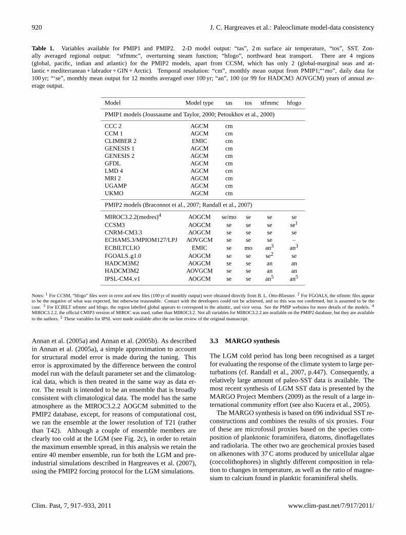
Table 1. Variables available for PMIP1 and PMIP2. 2-D model output: “tas”, 2 m surface air temperature, “tos”, SST. Zon-ally averaged regional output: “stfmmc”, overturning steam function; “hfogo”, northward heat transport. There are 4 regions(global, pacific, indian and atlantic) for the PMIP2 models, apart from CCSM, which has only 2 (global-marginal seas and at-lantic + mediterranean + labrador + GIN + Arctic). Temporal resolution: “cm”, monthly mean output from PMIP1;“‘mo”, daily data for100 yr; “‘se”, monthly mean output for 12 months averaged over 100 yr; “an”, 100 (or 99 for HADCM3 AOVGCM) years of annual av-erage output.

Model Model type tas tos stfmmc hfogo

PMIP1 models (Joussaume and Taylor, 2000; Petoukhov et al., 2000)

CCC 2 AGCM cmCCM 1 AGCM cmCLIMBER 2 EMIC cmGENESIS 1 AGCM cmGENESIS 2 AGCM cmGFDL AGCM cmLMD 4 AGCM cmMRI 2 AGCM cmUGAMP AGCM cmUKMO AGCM cm

PMIP2 models (Braconnot et al., 2007; Randall et al., 2007)

MIROC3.2.2(medres)4 AOGCM se/mo se se seCCSM3 AOGCM se se se se1

CNRM-CM3.3 AOGCM se se se seECHAM5.3/MPIOM127/LPJ AOVGCM se se se –ECBILTCLIO EMIC se mo an3 an3

FGOALS g1.0 AOGCM se se se2 seHADCM3M2 AOGCM se se an anHADCM3M2 AOVGCM se se an anIPSL-CM4 v1 AOGCM se se an5 an5

Notes:1 For CCSM, “hfogo” files were in error and new files (100 yr of monthly output) were obtained directly from B. L. Otto-Bliesner.2 For FGOALS, the stfmmc files appearto be the negative of what was expected, but otherwise reasonable. Contact with the developers could not be achieved, and so this was not confirmed, but is assumed to be thecase.3 For ECBILT stfmmc and hfogo, the region labelled global appears to correspond to the atlantic, and vice versa. See the PMIP websites for more details of the models.4

MIROC3.2.2, the official CMIP3 version of MIROC was used, rather than MIROC3.2. Not all variables for MIROC3.2.2 are available on the PMIP2 database, but they are availableto the authors.5 These variables for IPSL were made available after the on-line review of the original manuscript.

Annan et al.(2005a) andAnnan et al.(2005b). As describedin Annan et al.(2005a), a simple approximation to accountfor structural model error is made during the tuning. Thiserror is approximated by the difference between the controlmodel run with the default parameter set and the climatolog-ical data, which is then treated in the same way as data er-ror. The result is intended to be an ensemble that is broadlyconsistent with climatological data. The model has the sameatmosphere as the MIROC3.2.2 AOGCM submitted to thePMIP2 database, except, for reasons of computational cost,we ran the ensemble at the lower resolution of T21 (ratherthan T42). Although a couple of ensemble members areclearly too cold at the LGM (see Fig.2c), in order to retainthe maximum ensemble spread, in this analysis we retain theentire 40 member ensemble, run for both the LGM and pre-industrial simulations described inHargreaves et al.(2007),using the PMIP2 forcing protocol for the LGM simulations.

3.3 MARGO synthesis

The LGM cold period has long been recognised as a targetfor evaluating the response of the climate system to large per-turbations (cf.Randall et al., 2007, p.447). Consequently, arelatively large amount of paleo-SST data is available. Themost recent synthesis of LGM SST data is presented by theMARGO Project Members(2009) as the result of a large in-ternational community effort (see alsoKucera et al., 2005).

The MARGO synthesis is based on 696 individual SST re-constructions and combines the results of six proxies. Fourof these are microfossil proxies based on the species com-position of planktonic foraminifera, diatoms, dinoflagellatesand radiolaria. The other two are geochemical proxies basedon alkenones with 37 C atoms produced by unicellular algae(coccolithophores) in slightly different composition in rela-tion to changes in temperature, as well as the ratio of magne-sium to calcium found in planktic foraminiferal shells.



MARGO synthesis, LGM anomaly

MARGO synthesis, uncertainty in LGM anomaly

oC

(a)

(b)

oC

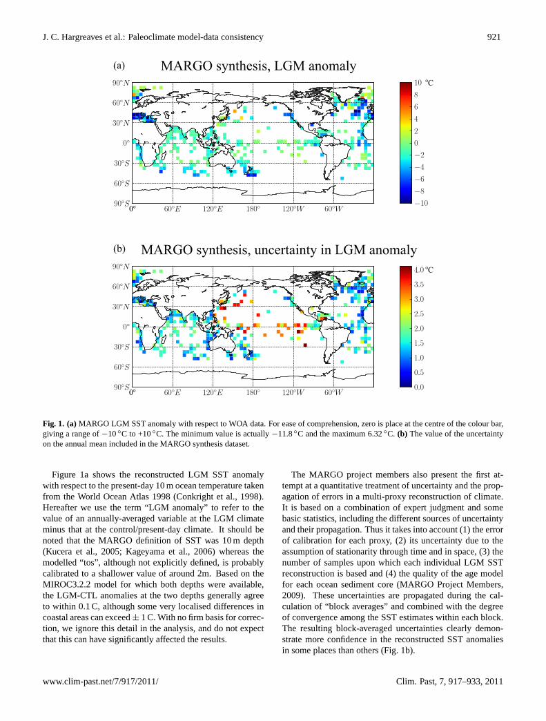
Fig. 1. (a)MARGO LGM SST anomaly with respect to WOA data. For ease of comprehension, zero is place at the centre of the colour bar,giving a range of−10◦C to +10◦C. The minimum value is actually−11.8◦C and the maximum 6.32◦C. (b) The value of the uncertaintyon the annual mean included in the MARGO synthesis dataset.

Figure 1a shows the reconstructed LGM SST anomalywith respect to the present-day 10 m ocean temperature takenfrom the World Ocean Atlas 1998 (Conkright et al., 1998).Hereafter we use the term “LGM anomaly” to refer to thevalue of an annually-averaged variable at the LGM climateminus that at the control/present-day climate. It should benoted that the MARGO definition of SST was 10 m depth(Kucera et al., 2005; Kageyama et al., 2006) whereas themodelled “tos”, although not explicitly defined, is probablycalibrated to a shallower value of around 2m. Based on theMIROC3.2.2 model for which both depths were available,the LGM-CTL anomalies at the two depths generally agreeto within 0.1 C, although some very localised differences incoastal areas can exceed± 1 C. With no firm basis for correc-tion, we ignore this detail in the analysis, and do not expectthat this can have significantly affected the results.

The MARGO project members also present the first at-tempt at a quantitative treatment of uncertainty and the prop-agation of errors in a multi-proxy reconstruction of climate.It is based on a combination of expert judgment and somebasic statistics, including the different sources of uncertaintyand their propagation. Thus it takes into account (1) the errorof calibration for each proxy, (2) its uncertainty due to theassumption of stationarity through time and in space, (3) thenumber of samples upon which each individual LGM SSTreconstruction is based and (4) the quality of the age modelfor each ocean sediment core (MARGO Project Members,2009). These uncertainties are propagated during the cal-culation of “block averages” and combined with the degreeof convergence among the SST estimates within each block.The resulting block-averaged uncertainties clearly demon-strate more confidence in the reconstructed SST anomaliesin some places than others (Fig.1b).



MARGOPMIP2 SSTPMIP2 TASPMIP1 TASJUMP SST

Latitude (o)

Tem

pera

ture

cha

nge

(o C)

Tem

pera

ture

cha

nge

(o C)

Global Ocean, LGM anomaly

(a)

(b)

Tem

pera

ture

cha

nge

(o C)

(c)

5

0

-5

-10

-15

-20

-25

0

-5

-10

-15

-20

-25

-30

-90 -60 -30 0 30 60 90

0

-2

-4

-6

-8

-10

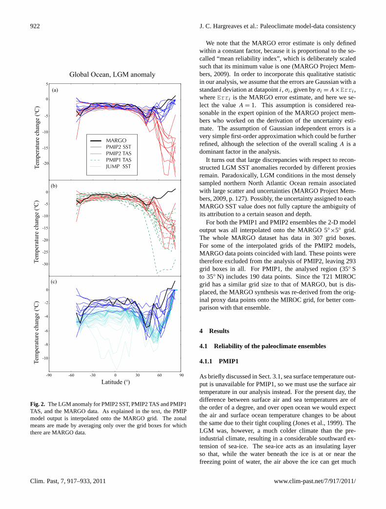
Fig. 2. The LGM anomaly for PMIP2 SST, PMIP2 TAS and PMIP1TAS, and the MARGO data. As explained in the text, the PMIPmodel output is interpolated onto the MARGO grid. The zonalmeans are made by averaging only over the grid boxes for whichthere are MARGO data.

We note that the MARGO error estimate is only definedwithin a constant factor, because it is proportional to the so-called “mean reliability index”, which is deliberately scaledsuch that its minimum value is one (MARGO Project Mem-bers, 2009). In order to incorporate this qualitative statisticin our analysis, we assume that the errors are Gaussian with astandard deviation at datapointi, σi , given byσi = A×Err i ,whereErr i is the MARGO error estimate, and here we se-lect the valueA = 1. This assumption is considered rea-sonable in the expert opinion of the MARGO project mem-bers who worked on the derivation of the uncertainty esti-mate. The assumption of Gaussian independent errors is avery simple first-order approximation which could be furtherrefined, although the selection of the overall scalingA is adominant factor in the analysis.

It turns out that large discrepancies with respect to recon-structed LGM SST anomalies recorded by different proxiesremain. Paradoxically, LGM conditions in the most denselysampled northern North Atlantic Ocean remain associatedwith large scatter and uncertainties (MARGO Project Mem-bers, 2009, p. 127). Possibly, the uncertainty assigned to eachMARGO SST value does not fully capture the ambiguity ofits attribution to a certain season and depth.

For both the PMIP1 and PMIP2 ensembles the 2-D modeloutput was all interpolated onto the MARGO 5◦

×5◦ grid.The whole MARGO dataset has data in 307 grid boxes.For some of the interpolated grids of the PMIP2 models,MARGO data points coincided with land. These points weretherefore excluded from the analysis of PMIP2, leaving 293grid boxes in all. For PMIP1, the analysed region (35◦ Sto 35◦ N) includes 190 data points. Since the T21 MIROCgrid has a similar grid size to that of MARGO, but is dis-placed, the MARGO synthesis was re-derived from the orig-inal proxy data points onto the MIROC grid, for better com-parison with that ensemble.

4 Results

4.1 Reliability of the paleoclimate ensembles

4.1.1 PMIP1

As briefly discussed in Sect.3.1, sea surface temperature out-put is unavailable for PMIP1, so we must use the surface airtemperature in our analysis instead. For the present day, thedifference between surface air and sea temperatures are ofthe order of a degree, and over open ocean we would expectthe air and surface ocean temperature changes to be aboutthe same due to their tight coupling (Jones et al., 1999). TheLGM was, however, a much colder climate than the pre-industrial climate, resulting in a considerable southward ex-tension of sea-ice. The sea-ice acts as an insulating layerso that, while the water beneath the ice is at or near thefreezing point of water, the air above the ice can get much



Area weighted

Rank of MARGO data in PMIP1 ensemble

Rank histogram Ensemble mean bias

Temperature (oC)Rank

(a)

(b) (c)

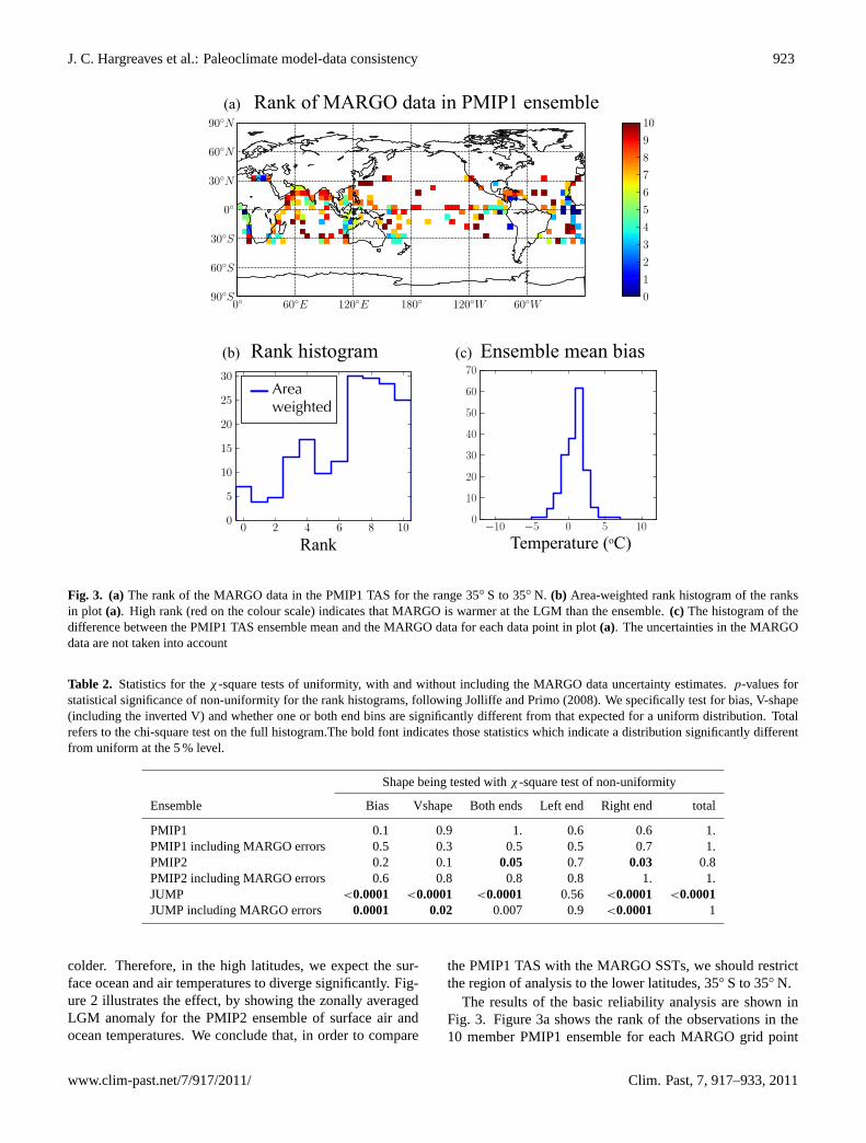
Fig. 3. (a)The rank of the MARGO data in the PMIP1 TAS for the range 35◦ S to 35◦ N. (b) Area-weighted rank histogram of the ranksin plot (a). High rank (red on the colour scale) indicates that MARGO is warmer at the LGM than the ensemble.(c) The histogram of thedifference between the PMIP1 TAS ensemble mean and the MARGO data for each data point in plot(a). The uncertainties in the MARGOdata are not taken into account

Table 2. Statistics for theχ -square tests of uniformity, with and without including the MARGO data uncertainty estimates.p-values forstatistical significance of non-uniformity for the rank histograms, followingJolliffe and Primo(2008). We specifically test for bias, V-shape(including the inverted V) and whether one or both end bins are significantly different from that expected for a uniform distribution. Totalrefers to the chi-square test on the full histogram.The bold font indicates those statistics which indicate a distribution significantly differentfrom uniform at the 5 % level.

Shape being tested withχ -square test of non-uniformity

Ensemble Bias Vshape Both ends Left end Right end total

PMIP1 0.1 0.9 1. 0.6 0.6 1.PMIP1 including MARGO errors 0.5 0.3 0.5 0.5 0.7 1.PMIP2 0.2 0.1 0.05 0.7 0.03 0.8PMIP2 including MARGO errors 0.6 0.8 0.8 0.8 1. 1.JUMP <0.0001 <0.0001 <0.0001 0.56 <0.0001 <0.0001JUMP including MARGO errors 0.0001 0.02 0.007 0.9 <0.0001 1

colder. Therefore, in the high latitudes, we expect the sur-face ocean and air temperatures to diverge significantly. Fig-ure2 illustrates the effect, by showing the zonally averagedLGM anomaly for the PMIP2 ensemble of surface air andocean temperatures. We conclude that, in order to compare

the PMIP1 TAS with the MARGO SSTs, we should restrictthe region of analysis to the lower latitudes, 35◦ S to 35◦ N.

The results of the basic reliability analysis are shown inFig. 3. Figure3a shows the rank of the observations in the10 member PMIP1 ensemble for each MARGO grid point



LGM anomaly (PMIP1 ensemble mean - MARGO)

LGM anomaly (PMIP2 ensemble mean - MARGO)

LGM anomaly (JUMP ensemble mean - MARGO)

oC

oC

oC

(a)

(b)

(c)

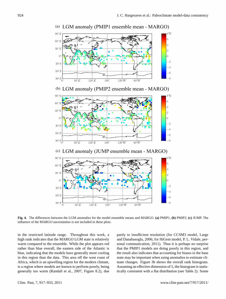
Fig. 4. The differences between the LGM anomalies for the model ensemble means and MARGO.(a) PMIP1,(b) PMIP2,(c) JUMP. Theinfluence of the MARGO uncertainties is not included in these plots.

in the restricted latitude range. Throughout this work, ahigh rank indicates that the MARGO LGM state is relativelywarm compared to the ensemble. While the plot appears redrather than blue overall, the eastern side of the Atlantic isblue, indicating that the models have generally more coolingin this region than the data. This area off the west coast ofAfrica, which is an upwelling region for the modern climate,is a region where models are known to perform poorly, beinggenerally too warm (Randall et al., 2007, Figure 8.2), due

partly to insufficient resolution (for CCSM3 model,Largeand Danabasoglu, 2006; for HiGem model, P. L. Vidale, per-sonal communication, 2011). Thus it is perhaps no surprisethat the PMIP1 models are doing poorly in this region, andthe result also indicates that accounting for biases in the basestate may be important when using anomalies to estimate cli-mate changes. Figure3b shows the overall rank histogram.Assuming an effective dimension of 5, the histogram is statis-tically consistent with a flat distribution (see Table2). Some



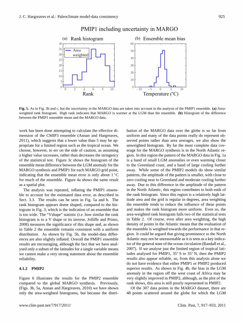
PMIP1 including uncertainty in MARGORank histogram Ensemble mean bias

Rank Temperature (oC)

Area weighted

(a) (b)

Fig. 5. As in Fig.3b and c, but the uncertainty in the MARGO data are taken into account in the analysis of the PMIP1 ensemble.(a) Area-weighted rank histogram. High rank indicates that MARGO is warmer at the LGM than the ensemble.(b) Histogram of the differencebetween the PMIP1 ensemble mean and the MARGO data.

work has been done attempting to calculate the effective di-mension of the CMIP3 ensemble (Annan and Hargreaves,2011), which suggests that a lower value than 5 may be ap-propriate for a limited region such as the tropical ocean. Wechoose, however, to err on the side of caution, as assuminga higher value increases, rather than decreases the stringencyof the statistical test. Figure3c shows the histogram of theensemble mean difference between the LGM anomaly for theMARGO synthesis and PMIP1 for each MARGO grid point,indicating that the ensemble mean error is only about 1◦Cfor much of the ensemble. Figure 4a shows the same resultas a spatial plot.

The analysis was repeated, inflating the PMIP1 ensem-ble to account for the estimated data error, as described inSect.3.3. The results can be seen in Fig.5a and b. Therank histogram appears dome shaped, compared to the his-togram in Fig.3, which is the indication of an ensemble thatis too wide. The “Vshape” statistic (i.e. how similar the rankhistogram is to a V shape or its inverse,Jolliffe and Primo,2008) measures the significance of this shape and, as shownin Table2 the ensemble remains consistent with a uniformdistribution. As shown by Fig.5b, the model-data differ-ences are also slightly inflated. Overall the PMIP1 ensembleresults are encouraging, although the fact that we have anal-ysed only a subset of the latitudes for a single variable meanswe cannot make a very strong statement about the ensemblereliability.

4.1.2 PMIP2

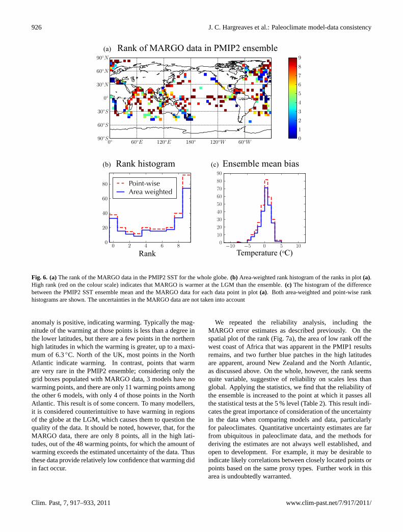
Figure 6 illustrates the results for the PMIP2 ensemblecompared to the global MARGO synthesis. Previously,(Figs.3b, 5a, Annan and Hargreaves, 2010) we have shownonly the area-weighted histograms, but because the distri-

bution of the MARGO data over the globe is so far fromuniform and many of the data points really do represent ob-served points rather than area averages, we also show theunweighted histogram. By far the most complete data cov-erage for the MARGO synthesis is in the North Atlantic re-gion. In this region the pattern of the MARGO data in Fig.1ais a band of small LGM anomalies or even warming closerto the Greenland coast, and a band of large cooling furtheraway. While some of the PMIP2 models do show similarpatterns, the amplitude of the pattern is smaller, with close tozero cooling near to Greenland and moderate cooling furtheraway. Due to this difference in the amplitude of the patternin the North Atlantic, this region contributes to both ends ofthe rank histogram. Since this region is a relatively high lat-itude area and the grid is regular in degrees, area weightingthe ensemble tends to reduce the influence of these pointsand makes the rank histogram more uniform. Even so, thearea-weighted rank histogram fails two of the statistical testsin Table2. Of course, even after area weighting, the highdensity of points in the Atlantic means that the evaluation ofthe ensemble is weighted towards the performance in that re-gion. It could be argued that giving prominence to the NorthAtlantic may not be unreasonable as it is seen as a key indica-tor of the general state of the ocean circulation (Randall et al.,2007). If we analyse just the limited region of tropical lati-tudes analysed for PMIP1, 35◦ S to 35◦ N, then the PMIP2results also appear reliable, so, from this analysis alone wedo not have evidence that either PMIP1 or PMIP2 producedsuperior results. As shown in Fig.4b, the bias in the LGManomaly in the region off the west coast of Africa may bevery slightly improved in PMIP2, although, as the plot of therank shows, this area is still poorly represented in PMIP2.

Of the 307 data points in the MARGO dataset, there are48 points scattered around the globe for which the LGM



Point-wiseArea weighted

Rank of MARGO data in PMIP2 ensemble



(a)

(b) (c)

Fig. 6. (a)The rank of the MARGO data in the PMIP2 SST for the whole globe.(b) Area-weighted rank histogram of the ranks in plot(a).High rank (red on the colour scale) indicates that MARGO is warmer at the LGM than the ensemble.(c) The histogram of the differencebetween the PMIP2 SST ensemble mean and the MARGO data for each data point in plot(a). Both area-weighted and point-wise rankhistograms are shown. The uncertainties in the MARGO data are not taken into account

anomaly is positive, indicating warming. Typically the mag-nitude of the warming at those points is less than a degree inthe lower latitudes, but there are a few points in the northernhigh latitudes in which the warming is greater, up to a maxi-mum of 6.3◦C. North of the UK, most points in the NorthAtlantic indicate warming. In contrast, points that warmare very rare in the PMIP2 ensemble; considering only thegrid boxes populated with MARGO data, 3 models have nowarming points, and there are only 11 warming points amongthe other 6 models, with only 4 of those points in the NorthAtlantic. This result is of some concern. To many modellers,it is considered counterintuitive to have warming in regionsof the globe at the LGM, which causes them to question thequality of the data. It should be noted, however, that, for theMARGO data, there are only 8 points, all in the high lati-tudes, out of the 48 warming points, for which the amount ofwarming exceeds the estimated uncertainty of the data. Thusthese data provide relatively low confidence that warming didin fact occur.

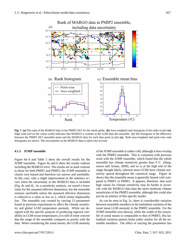
We repeated the reliability analysis, including theMARGO error estimates as described previously. On thespatial plot of the rank (Fig.7a), the area of low rank off thewest coast of Africa that was apparent in the PMIP1 resultsremains, and two further blue patches in the high latitudesare apparent, around New Zealand and the North Atlantic,as discussed above. On the whole, however, the rank seemsquite variable, suggestive of reliability on scales less thanglobal. Applying the statistics, we find that the reliability ofthe ensemble is increased to the point at which it passes allthe statistical tests at the 5 % level (Table2). This result indi-cates the great importance of consideration of the uncertaintyin the data when comparing models and data, particularlyfor paleoclimates. Quantitative uncertainty estimates are farfrom ubiquitous in paleoclimate data, and the methods forderiving the estimates are not always well established, andopen to development. For example, it may be desirable toindicate likely correlations between closely located points orpoints based on the same proxy types. Further work in thisarea is undoubtedly warranted.




Rank of MARGO data in PMIP2 ensemble, including data uncertainty



(a)

(b) (c)

Fig. 7. (a)The rank of the MARGO data in the PMIP2 SST for the whole globe.(b) Area-weighted rank histogram of the ranks in plot(a).High rank (red on the colour scale) indicates that MARGO is warmer at the LGM than the ensemble.(c) The histogram of the differencebetween the PMIP2 SST ensemble mean and the MARGO data for each data point in plot(a). Both area-weighted and point-wise rankhistograms are shown. The uncertainties in the MARGO data is taken into account

4.1.3 JUMP ensemble

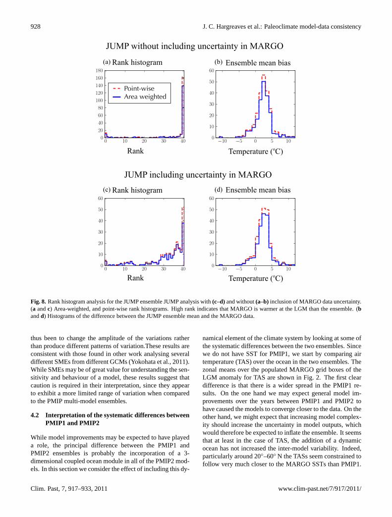
Figure 8a–d and Table2 show the overall results for theJUMP ensemble. Figure8a and b show the results withoutincluding the MARGO error. The results are in stark contrastto those for both PMIP1 and PMIP2; the JUMP ensemble isclearly very biased and therefore too narrow and unreliable.In this case, only a slight improvement in the statistics oc-curs when the uncertainty in the MARGO data is included(Fig. 8c and d). As a sensitivity analysis, we tested a lowervalue for the assumed effective dimension, but the ensembleremains unreliable unless the assumed effective dimensionis reduced to a value as low as 2, which seems implausiblylow. The ensemble was created by varying 13 parametersfound in previous experiments to affect the climate sensitiv-ity and global LGM temperature anomaly. While not de-signed with the specific purpose of producing regional vari-ability in LGM ocean temperatures, it is still of some concernthat the range of the ensemble compares so poorly with thedata. When considering the zonal means, the LGM anomaly

of the JUMP ensemble is rather cold, although it does overlapwith the PMIP2 ensemble. This is consistent with previouswork with the JUMP ensemble, which found that the wholeensemble has climate sensitivity greater than 4◦C (Harg-reaves and Annan, 2009), and so is at the high end of therange thought likely, whereas most GCMs have climate sen-sitivity spread throughout the canonical range. Figure4cshows that the ensemble mean is generally biased cold com-pared to PMIP1 or PMIP2. It appears, therefore, that suchhigh values for climate sensitivity may be harder to recon-cile with the MARGO data than the more moderate climatesensitivities of the PMIP2 ensemble, although this could alsojust be an artefact of this specific model.

As can be seen in Fig.2c, there is considerable variationbetween ensemble members in the latitudinal variation of thezonal mean LGM anomaly in the PMIP2 ensemble. For theJUMP ensemble (not shown), while the width of the ensem-ble of zonal means is comparable to that of PMIP2, this lat-itudinal variation pattern looks rather similar for all the en-semble members. The effect of varying the parameters has



JUMP without including uncertainty in MARGO

JUMP including uncertainty in MARGO






(a) (b)

(c) (d)

Fig. 8. Rank histogram analysis for the JUMP ensemble JUMP analysis with(c–d)and without(a–b) inclusion of MARGO data uncertainty.(a andc) Area-weighted, and point-wise rank histograms. High rank indicates that MARGO is warmer at the LGM than the ensemble. (bandd) Histograms of the difference between the JUMP ensemble mean and the MARGO data.

thus been to change the amplitude of the variations ratherthan produce different patterns of variation.These results areconsistent with those found in other work analysing severaldifferent SMEs from different GCMs (Yokohata et al., 2011).While SMEs may be of great value for understanding the sen-sitivity and behaviour of a model, these results suggest thatcaution is required in their interpretation, since they appearto exhibit a more limited range of variation when comparedto the PMIP multi-model ensembles.

4.2 Interpretation of the systematic differences betweenPMIP1 and PMIP2

While model improvements may be expected to have playeda role, the principal difference between the PMIP1 andPMIP2 ensembles is probably the incorporation of a 3-dimensional coupled ocean module in all of the PMIP2 mod-els. In this section we consider the effect of including this dy-

namical element of the climate system by looking at some ofthe systematic differences between the two ensembles. Sincewe do not have SST for PMIP1, we start by comparing airtemperature (TAS) over the ocean in the two ensembles. Thezonal means over the populated MARGO grid boxes of theLGM anomaly for TAS are shown in Fig.2. The first cleardifference is that there is a wider spread in the PMIP1 re-sults. On the one hand we may expect general model im-provements over the years between PMIP1 and PMIP2 tohave caused the models to converge closer to the data. On theother hand, we might expect that increasing model complex-ity should increase the uncertainty in model outputs, whichwould therefore be expected to inflate the ensemble. It seemsthat at least in the case of TAS, the addition of a dynamicocean has not increased the inter-model variability. Indeed,particularly around 20◦–60◦ N the TASs seem constrained tofollow very much closer to the MARGO SSTs than PMIP1.



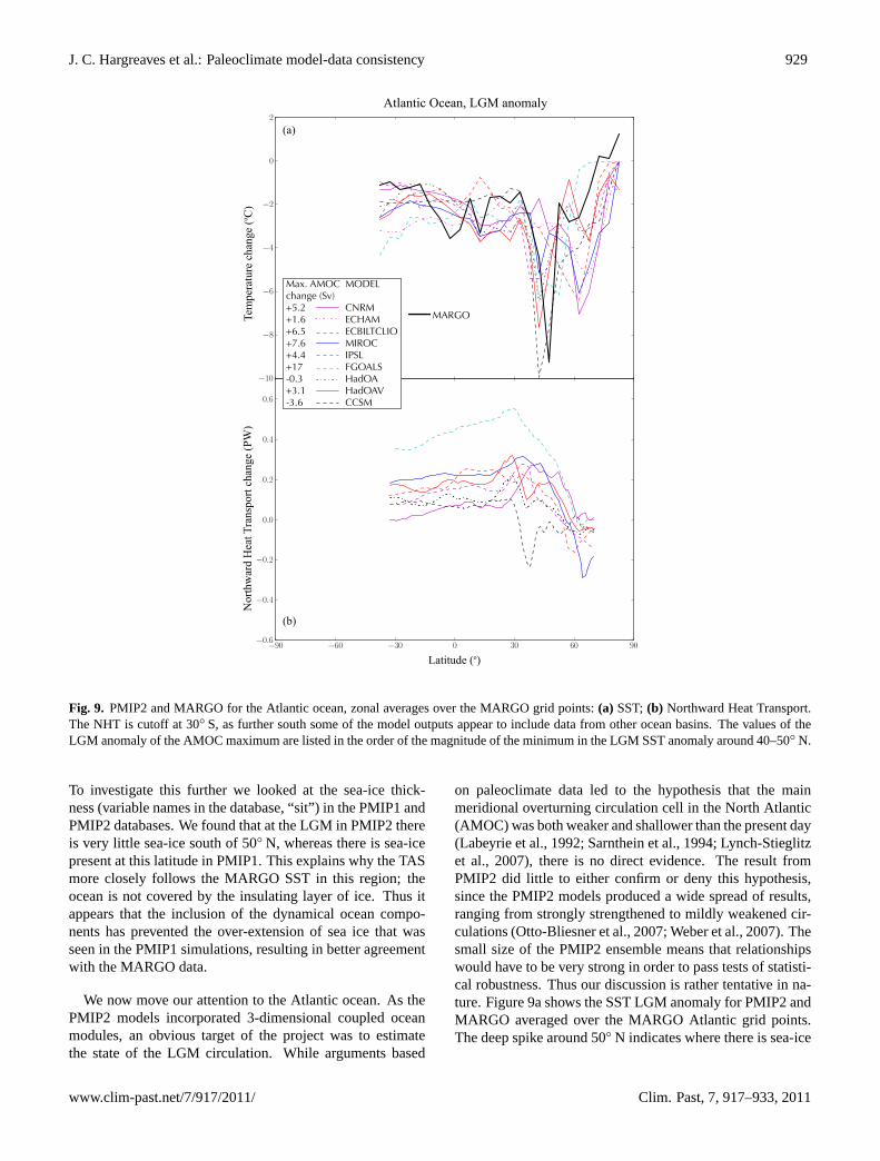
Max. AMOC MODELchange (Sv)+5.2 CNRM +1.6 ECHAM +6.5 ECBILTCLIO +7.6 MIROC +4.4 IPSL +17 FGOALS -0.3 HadOA +3.1 HadOAV -3.6 CCSM

MARGO

Atlantic Ocean, LGM anomaly

Nor

thw

ard

Hea

t Tra

nspo

rt ch

ange

(PW

)Te

mpe

ratu

re c

hang

e (o C

)

(a)

(b)

Latitude (o)

Fig. 9. PMIP2 and MARGO for the Atlantic ocean, zonal averages over the MARGO grid points:(a) SST;(b) Northward Heat Transport.The NHT is cutoff at 30◦ S, as further south some of the model outputs appear to include data from other ocean basins. The values of theLGM anomaly of the AMOC maximum are listed in the order of the magnitude of the minimum in the LGM SST anomaly around 40–50◦ N.

To investigate this further we looked at the sea-ice thick-ness (variable names in the database, “sit”) in the PMIP1 andPMIP2 databases. We found that at the LGM in PMIP2 thereis very little sea-ice south of 50◦ N, whereas there is sea-icepresent at this latitude in PMIP1. This explains why the TASmore closely follows the MARGO SST in this region; theocean is not covered by the insulating layer of ice. Thus itappears that the inclusion of the dynamical ocean compo-nents has prevented the over-extension of sea ice that wasseen in the PMIP1 simulations, resulting in better agreementwith the MARGO data.

We now move our attention to the Atlantic ocean. As thePMIP2 models incorporated 3-dimensional coupled oceanmodules, an obvious target of the project was to estimatethe state of the LGM circulation. While arguments based

on paleoclimate data led to the hypothesis that the mainmeridional overturning circulation cell in the North Atlantic(AMOC) was both weaker and shallower than the present day(Labeyrie et al., 1992; Sarnthein et al., 1994; Lynch-Stieglitzet al., 2007), there is no direct evidence. The result fromPMIP2 did little to either confirm or deny this hypothesis,since the PMIP2 models produced a wide spread of results,ranging from strongly strengthened to mildly weakened cir-culations (Otto-Bliesner et al., 2007; Weber et al., 2007). Thesmall size of the PMIP2 ensemble means that relationshipswould have to be very strong in order to pass tests of statisti-cal robustness. Thus our discussion is rather tentative in na-ture. Figure9a shows the SST LGM anomaly for PMIP2 andMARGO averaged over the MARGO Atlantic grid points.The deep spike around 50◦ N indicates where there is sea-ice



max. North Atlantic MOC (Sv)

max. North Atlantic MOC (Sv)

max. North Atlantic NHT (PW)

max

. Nor

th A

tlant

ic N

HT

(PW

)R

MSE

of S

ST v

s MA

RG

OR

MSE

of S

ST v

s MA

RG

O

corr.coef. = 0.94

corr.coef. = 0.27

corr.coef. = 0.22

(a)

(b)

(c)

ECBILTCLIO CCSMCNRM FGOALSHadOA IPSL HadOAV ECHAM MIROC

Fig. 10. Correlation between: the root mean square of the differ-ence in Atlantic SST between PMIP2 and MARGO scaled by theMARGO uncertainty; the maximum northward heat transport inthe North Atlantic; and the maximum meridional overturning in theNorth Atlantic.

for the LGM but not the present day, since the area furthernorth where there is sea-ice for both periods does not coolso much at the LGM due to the insulating properties of thesea-ice. On the whole, the models reproduce this spike inqualitative terms, but the magnitude varies. The location ofthe spike for those models with a single clear sharp spike atclose to the correct latitude tends to be a little to the south. Inthe box on the same Figure are shown the maximum AMOCanomalies for the PMIP2 models. Three of the four mod-els with the smallest maximum AMOC anomalies have thedeepest spikes, closest to the observations. Figure9b showsthat the Northward Heat Transport (NHT) in the Atlantic isincreased at the LGM at least as far as 30◦ N for all 8 of thePMIP2 models for which this variable is available. This isanother systematic difference caused by adding the dynam-ical ocean; the PMIP1 slab-ocean models impose the sameoceanic heat transport, so the LGM anomaly for NorthwardHeat Transport is fixed at zero. This systematic difference(consistent with the results ofMurakami et al., 2008) indi-cates that, irrelevant of the AMOC, the dynamical ocean iscompensating for the cooling in the northern high latitudesby transporting more heat northward at the LGM. This seemsa natural consequence of the greater latitudinal temperaturegradient, since it implies that a given volume transport willcarry more heat from the tropics to high latitudes than it doesin the control climate.

In order to quantitatively compare the models and data,we also calculate the normalised area-weighted root meansquare error (RMSE) in the Atlantic for MARGO and PMIP2LGM anomalies for SST. We weight each squared modeldata difference by the appropriate grid box area and nor-malise by the relevant MARGO uncertainty (squared) in or-der to generate a nondimensional value. We then comparethe values obtained to the maximum AMOC and maximumNHT anomalies for the North Atlantic, by correlation. Theresults are shown in Fig.10. Most of the models have anRMSE around 1.7–1.9, but the IPSL model has much lowererror of 1.35. As argued byAnnan and Hargreaves(2011)it is generally expected that, depending on the dimension ofthe ensemble, the ensemble mean may outperform many en-semble members. In this case only the IPSL model is better;the RMSE of the ensemble mean is 1.46. The AMOC-RMSEand NHT-RMSE correlations are both positive, although notstatistically significant for such a small ensemble. The cor-relation between AMOC and NHT is, however, strong andstatistically significant. To sum up: in comparison to PMIP1,all the PMIP2 models have increased NHT in the Atlanticat least as far as 30◦ N; those with a larger increase in NHTalso have a larger increase in AMOC at the LGM, but there isweak evidence that a smaller change in NHT and AMOC ispreferred for a good fit to the MARGO data. A significantlylarger ensemble size (20–40 members) would be required forrobust results to be obtained for the AMOC-RMSE and NHT-RMSE relationships.



5 Conclusions

We have analysed the reliability of two PMIP ensembles andone single-model ensemble using the MARGO sea surfacetemperature data synthesis for the Last Glacial Maximum.Within the constraint that for PMIP1 only air temperaturedata can be analysed and this only for the lower latitudes,due to the unavailability of sea surface temperature data, wefind that neither ensemble is shown to give unreliable predic-tions of the MARGO data. The PMIP2 ensemble is some-what narrower than that of PMIP1, but once the uncertaintyin the MARGO data is taken into account, there is no indica-tion that it is too narrow. Rather it seems that model develop-ment including the addition of the coupled dynamical oceansin PMIP2 have caused the ensemble to be improved. Thiswork indicates the vital importance of including uncertaintyestimates along-side paleoclimate data. If we had not hadthe error estimate, we might have falsely concluded that thePMIP2 ensemble is too narrow. Further work to better modelthe data uncertainty estimate would be valuable for analysessuch as these.

The JUMP ensemble is found to be extremely unreli-able, even when the MARGO data uncertainty is includedin the analysis. This result is consistent with ongoing workanalysing several single model ensembles for the present day(Yokohata et al., 2011). It would appear that, in order to sam-ple as wide a range as the multi-model ensembles, a muchbroader range of parametric changes would need to be varied,which would be computationally problematical. Comparingthe JUMP and PMIP2 ensembles supports our previous con-clusion (Annan et al., 2005b), that the JUMP climate sensi-tivities of greater than 4◦C are less consistent with the datathan the generally lower climate sensitivities of the PMIP2models.

Comparison of the PMIP2 and PMIP1 ensembles revealsthat the addition of the coupled ocean models in PMIP2 havecaused systematic differences in the modelled LGM state.It can be inferred from the surface air temperatures that thePMIP2 ensemble is probably more consistent with the datain the high latitudes than PMIP1. There is a less south-ward extension of sea-ice with the PMIP2 models; the dy-namical oceans are causing northward heat transport to beincreased at least as far as 30◦ N. Despite these systematicdifferences, and a general narrowing of the ensemble, thereis a wide range of AMOC strength in the PMIP2 models.Stronger AMOC LGM anomaly correlates with stronger At-lantic northward heat transport LGM anomaly. There is alsoweak evidence for the PMIP2 models with lower AMOC(and NHT) LGM anomaly being more consistent with thedata, which would also be consistent with the observationallyderived estimates of the AMOC LGM anomaly. The ensem-ble size is not, however, sufficiently large to draw confidentconclusions, and so it is important that this is increased to en-able robust characterisation of the climate system behaviour.

The ensemble size for the LGM is expected to increase con-siderably over the next few years, as the PMIP3/CMIP5 runsbecome available. Increasing the robustness of these resultwould also be helped by having available data representativeof a range of variables including in the ocean at depth ratherthan only the surface, and initiatives are underway to increasethe scope of ocean data syntheses (Paul and Mulitza, 2009).

Acknowledgements.We are grateful to the three reviewers,C. J. Van Meerbeeck, M. Kucera and T. L. Edwards, whose carefulconsideration and helpful comments have enabled us to greatlyimprove the manuscript. This work was supported by the S-5-1project of the MoE, Japan, the Kakushin Program of MEXT,Japan, and by the DFG-Research Center/ Cluster of Excellence“The Ocean in the Earth System”, Germany. We acknowledgethe modelling groups involved in PMIP and PMIP2 in makingavailable the multi-model datasets, and the MIROC developmentteam in particular.

Edited by: V. Rath

References

Anderson, J.: A method for producing and evaluating probabilisticforecasts from ensemble model integrations, J. Climate, 9, 1518–1530, 1996.

Annan, J. D. and Hargreaves, J. C.: Reliability of theCMIP3 ensemble, Geophys. Res. Lett., 37, L02703,doi:10.1029/2009GL041994, 2010.

Annan, J. D. and Hargreaves, J. C.: Understanding the CMIP3multi-model ensemble, J. Climate, in press, 2011.

Annan, J. D., Hargreaves, J. C., Edwards, N. R., and Marsh, R.:Parameter estimation in an intermediate complexity Earth Sys-tem Model using an ensemble Kalman filter, Ocean Model., 8,135–154, 2005a.

Annan, J. D., Hargreaves, J. C., Ohgaito, R., Abe-Ouchi, A., andEmori, S.: Efficiently constraining climate sensitivity with pale-oclimate simulations, SOLA, 1, 181–184, 2005b.

Braconnot, P., Otto-Bliesner, B., Harrison, S., Joussaume, S., Pe-terchmitt, J.-Y., Abe-Ouchi, A., Crucifix, M., Driesschaert, E.,Fichefet, Th., Hewitt, C. D., Kageyama, M., Kitoh, A., Laıne,A., Loutre, M.-F., Marti, O., Merkel, U., Ramstein, G., Valdes,P., Weber, S. L., Yu, Y., and Zhao, Y.: Results of PMIP2 coupledsimulations of the Mid-Holocene and Last Glacial Maximum -Part 1: experiments and large-scale features, Clim. Past, 3, 261–277,doi:10.5194/cp-3-261-2007, 2007.

Claussen, M., Mysak, L., Weaver, A., Crucifix, M., Fichefet, T.,Loutre, M., Weber, S., Alcamo, J., Alexeev, V., Berger, A.,Calov, R., Ganopolski, A., Goosse, H., Lohmann, G., Lunkeit,F., Mokhov, I. I., Petoukhov, V., Stone, P., and Wang, Z.: Earthsystem models of intermediate complexity: closing the gap in thespectrum of climate system models, Clim. Dynam., 18, 579–586,2002.

Conkright, M., Levitus, S., OBrien, T., Boyer, T., Antonov, J., andStephens, C.: World ocean atlas 1998 CD-ROM data set docu-mentation, National Oceanographic Data Center (NODC) Inter-nal Report, Silver Spring, Maryland, 1998.


http://dx.doi.org/10.1029/2009GL041994

http://dx.doi.org/10.5194/cp-3-261-2007


Hamill, T.: Interpretation of rank histograms for verifying ensembleforecasts, Mon. Weather Rev., 129, 550–560, 2001.

Hargreaves, J. C.: Skill and uncertainty in climate models, Wi-ley Interdisciplinary Reviews, Climatic Change, 1, 556–564,doi:10.1002/wcc.58, 2010.

Hargreaves, J. C. and Annan, J. D.: On the importance of pale-oclimate modelling for improving predictions of future climatechange, Clim. Past, 5, 803–814,doi:10.5194/cp-5-803-2009,2009.

Hargreaves, J. C., Abe-Ouchi, A., and Annan, J. D.: Linking glacialand future climates through an ensemble of GCM simulations,Clim. Past, 3, 77–87,doi:10.5194/cp-3-77-2007, 2007.

Hasumi, H. and Emori, S.: K-1 coupled model (MIROC) descrip-tion, K-1 technical report 1, Tech. rep., Center for Climate Sys-tem Research, University of Tokyo, 2004.

Jolliffe, I. and Primo, C.: Evaluating Rank Histograms Using De-compositions of the Chi-Square Test Statistic, Mon. WeatherRev., 136, 2133–2139, 2008.

Jones, P., New, M., Parker, D., Martin, S., and Rigor, I.: Surface airtemperature and its changes over the past 150 years, Rev. Geo-phys., 37, 173–199, 1999.

Joussaume, S. and Taylor, K.: The Paleoclimate Modeling Inter-comparison Project, in: Paleoclimate Modelling IntercomparisonProject (PMIP): proceedings of the third PMIP workshop, editedby: Braconnot, P., Canada, 1999, 43–50, 2000.

Kageyama, M., Laine, A., Abe-Ouchi, A., Braconnot, P., Cortijo,E., Crucifix, M., Vernal, A. D., Guiot, J., Hewitt, C. D., Ki-toh, A., Kucera, M., Marti, O., Ohgaito, R., Otto-Bliesner, B.,Peltier, W. R., Rosell-Mele, A., Vettoretti, G., Weber, S. L.,and Yu, Y.: Last Glacial Maximum temperatures over the NorthAtlantic, Europe and western Siberia: a comparison betweenPMIP models, MARGO sea-surface temperatures and pollen-based reconstructions, Quaternary Sci. Rev., 25, 2082–2102,doi:10.1016/j.quascirev.2006.02.010, 2006.

Kucera, M., Rosell-Mele, A., Schneider, R., Waelbroeck, C., andWeinelt, M.: Multiproxy approach for the reconstruction of theglacial ocean surface (MARGO), Quaternary Sci. Rev., 24, 813–819, 2005.

Labeyrie, L., Duplessy, J., Duprat, J., Juilletleclerc, A., Moyes, J.,Michel, E., Kallel, N., and Shackleton, N.: Changes in the ver-tical structure of the north-Atlantic ocean between glacial andmodern times, Quaternary Sci. Rev., 11, 401–413, 1992.

Large, W. and Danabasoglu, G.: Attribution and impacts of upper-ocean biases in CCSM3, J. Climate, 19, 2325–2346, 2006.

Lynch-Stieglitz, J., Adkins, J. F., Curry, W. B., Dokken, T., Hall,I. R., Herguera, J. C., Hirschi, J. J.-M., Ivanova, E. V., Kissel, C.,Marchal, O., Marchitto, T. M., Mccave, I. N., Mcmanus, J. F.,Mulitza, S., Ninnemann, U., Peeters, F., Yu, E.-F., and Zahn,R.: Atlantic Meridional Overturning Circulation During the LastGlacial Maximum, Science, 316, 66–69, 2007.

MARGO Project Members: Constraints on the magnitude andpatterns of ocean cooling at the Last Glacial Maximum, Nat.Geosci., 2, 127–132,doi:10.1038/NGEO411, 2009.

Meehl, G., Covey, C., Delworth, T., Latif, M., McAvaney, B.,Mitchell, J., Stouffer, R., and Taylor, K.: The WCRP CMIP3multimodel dataset, B. Am. Meteorol. Soc, 88, 1383–1394,2007.

Murakami, S., Ohgaito, R., Abe-Ouchi, A., Crucifix, M., and Otto-Bliesner, B. L.: Global-Scale Energy and Freshwater Balance in

Glacial Climate: A Comparison of Three PMIP2 LGM Simula-tions, J. Climate, 21, 5008–5033, 2008.

Ohgaito, R. and Abe-Ouchi, A.: The role of ocean thermodynam-ics and dynamics in Asian summer monsoon changes during themid-Holocene, Clim. Dynam., 29, 39–50, 2007.

Otto-Bliesner, B. L., Hewitt, C. D., Marchitto, T. M., Brady, E.,Abe-Ouchi, A., Crucifix, M., Murakami, S., and Weber, S. L.:Last Glacial Maximum ocean thermohaline circulation: PMIP2model intercomparisons and data constraints, Geophys. Res.Lett., 34, L12706,doi:10.1029/2007GL029475, 2007.

Otto-Bliesner, B. L., Schneider, R., Brady, E., Kucera, M., Abe-Ouchi, A., Bard, E., Braconnot, P., Crucifix, M., Hewitt, C., andKageyama, M.: A comparison of PMIP2 model simulations andthe MARGO proxy reconstruction for tropical sea surface tem-peratures at last glacial maximum, Clim. Dynam., 32, 799–815,2009.

Paul, A. and Mulitza, S.: Challenges to Understanding Ocean Cir-culation During the Last Glacial Maximum, Eos, 90(19), p. 169,2009.

Petoukhov, V., Ganopolski, A., Brovkin, V., Claussen, M., Eliseev,A., Kubatzki, C., and Rahmstorf, S.: CLIMBER-2: a climatesystem model of intermediate complexity. Part I: model descrip-tion and performance for present climate, Clim. Dynam., 16, 1–17, 2000.

Randall, D. A., Wood, R., Bony, S., Colman, R., Fichefet, T., Fyfe,J., Kattsov, V., Pitman, A., Shukla, J., Srinivasan, J., Stouffer, R.,Sumi, A., and Taylor, K.: Climate Models and Their Evaluation,in: Climate Change 2007: The Physical Science Basis. Contri-bution of Working Group I to the Fourth Assessment Report ofthe Intergovernmental Panel on Climate Change, chap. 8, Cam-bridge University Press, Cambridge, United Kingdom and NewYork, NY, USA, 2007.

Sarnthein, M., Winn, K., Jung, S., Duplessy, J., Labeyrie, L., Er-lenkeuser, H., and Ganssen, G.: Changes in east Atlantic deep-water circulation over the last 30,000 years – 8 time slice recon-structions, Paleoceanography, 9, 209–267, 1994.

Solomon, S., Qin, D., Manning, M., Chen, Z., Marquis, M., Averyt,K., Tignor, M., and Miller, H. (Eds.): IPCC, 2007: Summary forPolicymakers, in: Climate Change 2007: The Physical ScienceBasis. Contribution of Working Group I to the Fourth Assess-ment Report of the Intergovernmental Panel on Climate Change,Cambridge University Press, Cambridge, United Kingdom andNew York, NY, USA, 2007.

Talagrand, O., Vautard, R., and Strauss, B.: Evaluation of proba-bilistic prediction systems, in: Proc. ECMWF Workshop on Pre-dictability, 1–25, 1997.

Weber, S.: The utility of Earth system Models of Intermediate Com-plexity (EMICs), WIRES Climate Change, 1, 234–252, 2010.

Weber, S. L., Drijfhout, S. S., Abe-Ouchi, A., Crucifix, M., Eby, M.,Ganopolski, A., Murakami, S., Otto-Bliesner, B., and Peltier, W.R.: The modern and glacial overturning circulation in the At-lantic ocean in PMIP coupled model simulations, Clim. Past, 3,51–64,doi:10.5194/cp-3-51-2007, 2007.

Yokohata, T., Webb, M., Collins, M., Williams, K. D., Yoshimori,M., Hargreaves, J. C., and Annan, J. D.: Structural similaritiesand differences in climate responses to CO2 increase betweentwo perturbed physics ensembles by general circulation models,J. Climate, 23, 1392–1410, 2010.

Yokohata, T., Annan, J., Collins, M., Jackson, C., Tobis, M., Webb,


http://dx.doi.org/10.1002/wcc.58

http://dx.doi.org/10.5194/cp-5-803-2009

http://dx.doi.org/10.5194/cp-3-77-2007

http://dx.doi.org/10.1016/j.quascirev.2006.02.010

http://dx.doi.org/10.1038/NGEO411

http://dx.doi.org/10.1029/2007GL029475

http://dx.doi.org/10.5194/cp-3-51-2007


M. J., and Hargreaves, J. C.: Reliability of multi-model andstructurally different single-model ensembles, Clim. Dynam.,submitted, 2011.

Yoshimori, M., Hargreaves, J., Annan, J., Yokohata, T., and Abe-Ouchi, A.: Dependency of Feedbacks on Forcing and ClimateState in Perturbed Parameter Ensembles, J. Climate, in press,2011.


copernicus cp-7-917-2011

Documents