Copulas ? What copulas ?

R. Chicheportiche & J.P. Bouchaud, CFM

Multivariate linear correlations

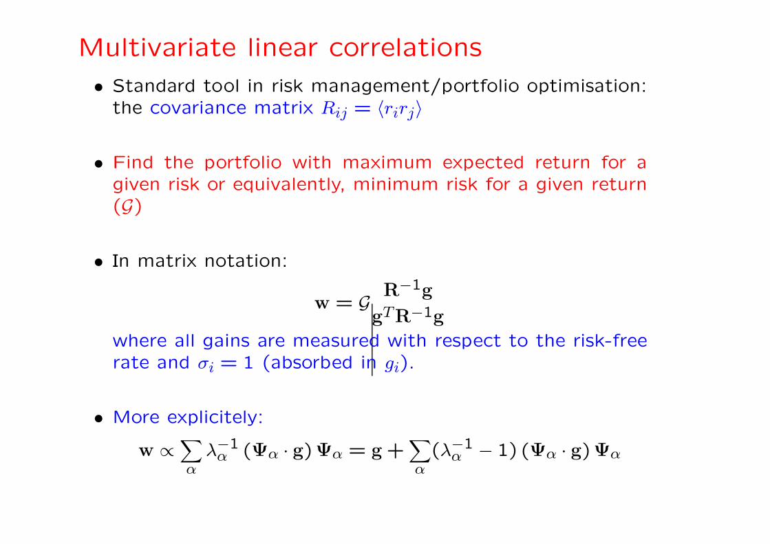
• Standard tool in risk management/portfolio optimisation:the covariance matrix Rij = 〈rirj〉

• Find the portfolio with maximum expected return for agiven risk or equivalently, minimum risk for a given return(G)

• In matrix notation:

w = GR−1g

gTR−1g

where all gains are measured with respect to the risk-freerate and σi = 1 (absorbed in gi).

• More explicitely:

w ∝∑

αλ−1

α (Ψα · g)Ψα = g +∑

α(λ−1

α − 1) (Ψα · g)Ψα

Multivariate non-linear correlations

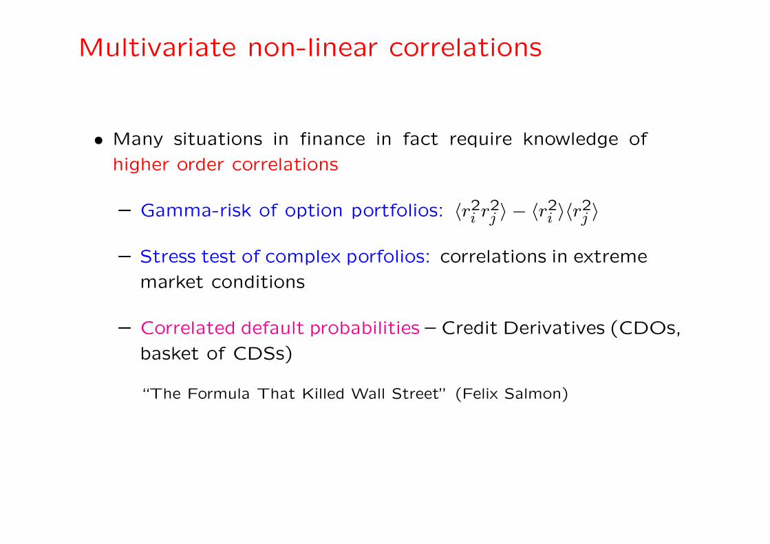
• Many situations in finance in fact require knowledge of

higher order correlations

– Gamma-risk of option portfolios: 〈r2i r2j 〉 − 〈r2i 〉〈r2j 〉

– Stress test of complex porfolios: correlations in extreme

market conditions

– Correlated default probabilities – Credit Derivatives (CDOs,

basket of CDSs)

“The Formula That Killed Wall Street” (Felix Salmon)

Different correlation coefficients

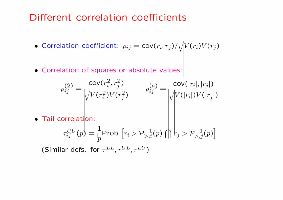
• Correlation coefficient: ρij = cov(ri, rj)/√

V (ri)V (rj)

• Correlation of squares or absolute values:

ρ(2)ij =

cov(r2i , r2j )√

V (r2i )V (r2j )ρ(a)ij =

cov(|ri|, |rj|)√

V (|ri|)V (|rj|)

• Tail correlation:

τUUij (p) =

1

pProb.

[

ri > P−1>,i(p)

⋂

rj > P−1>,j(p)

]

(Similar defs. for τLL, τUL, τLU)

Copulas

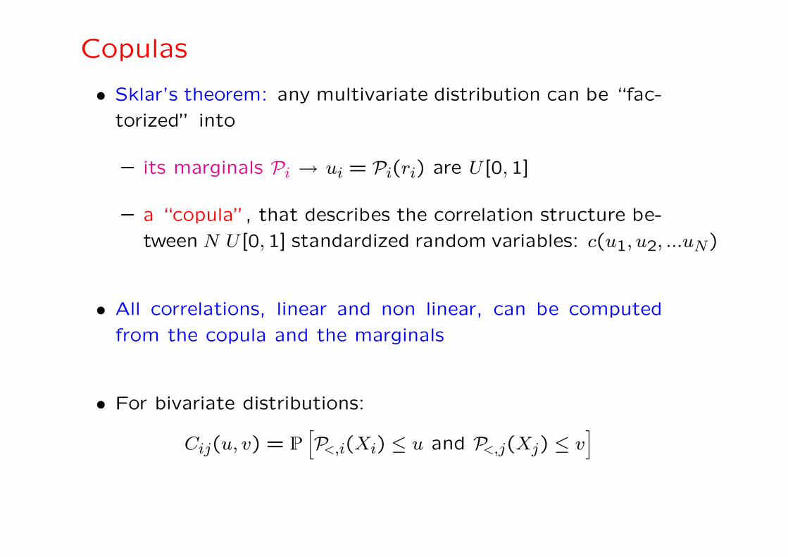
• Sklar’s theorem: any multivariate distribution can be “fac-

torized” into

– its marginals Pi → ui = Pi(ri) are U [0,1]

– a “copula”, that describes the correlation structure be-

tween N U [0,1] standardized random variables: c(u1, u2, ...uN)

• All correlations, linear and non linear, can be computed

from the copula and the marginals

• For bivariate distributions:

Cij(u, v) = P

[

P<,i(Xi) ≤ u and P<,j(Xj) ≤ v]

Copulas – Examples

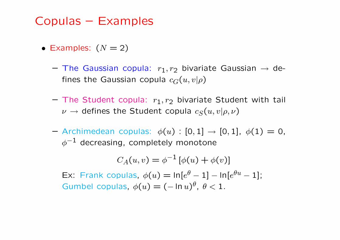
• Examples: (N = 2)

– The Gaussian copula: r1, r2 bivariate Gaussian → de-

fines the Gaussian copula cG(u, v|ρ)

– The Student copula: r1, r2 bivariate Student with tail

ν → defines the Student copula cS(u, v|ρ, ν)

– Archimedean copulas: φ(u) : [0,1] → [0,1], φ(1) = 0,

φ−1 decreasing, completely monotone

CA(u, v) = φ−1 [φ(u) + φ(v)]

Ex: Frank copulas, φ(u) = ln[eθ − 1] − ln[eθu − 1];

Gumbel copulas, φ(u) = (− lnu)θ, θ < 1.

The Copula red-herring

• Sklar’s theorem: a nearly empty shell – almost any c(u1, u2, ...uN)

with required properties is allowed.

• The usual financial mathematics syndrom: choose a class

of copulas – sometimes absurd – with convenient mathe-

matical properties and brute force calibrate to data

• If something fits it can’t be bad (??) Statistical tests

are not enough – intuition & plausible interpretation are

required

• But he does not wear any clothes! – see related comments

by Thomas Mikosch

The Copula red-herring

• Example 1: why on earth choose the Gaussian copula to

describe correlation between (positive) default times???

• Example 2: Archimedean copulas: take two U [0,1] ran-

dom variables s, w. Set t = K−1(w) with K(t) = t −

φ(t)/φ′(t).

u = φ−1 [sφ(t)] ; v = φ−1 [(1 − s)φ(t)] ; −→ r1, r2

Financial interpretation ???

• Models should reflect some plausible underlying structure

or mechanism

Copulas ? What copulas ?

• Aim of this work

– Develop intuition around copulas

– Identify empirical stylized facts about multivariate cor-

relations that copulas should reproduce

– Discuss “self-copulas” as a tool to study empirical tem-

poral dependences

– Propose an intuitively motivated, versatile model to

generate a wide class of non-linear correlations

Copulas

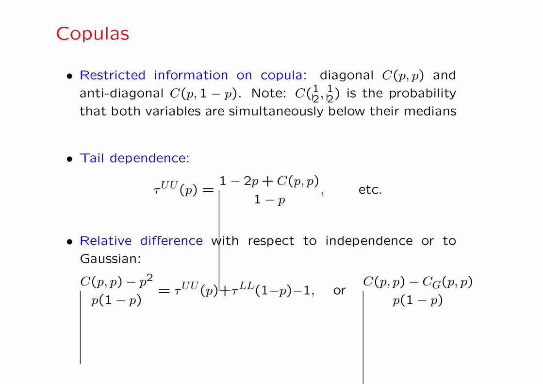
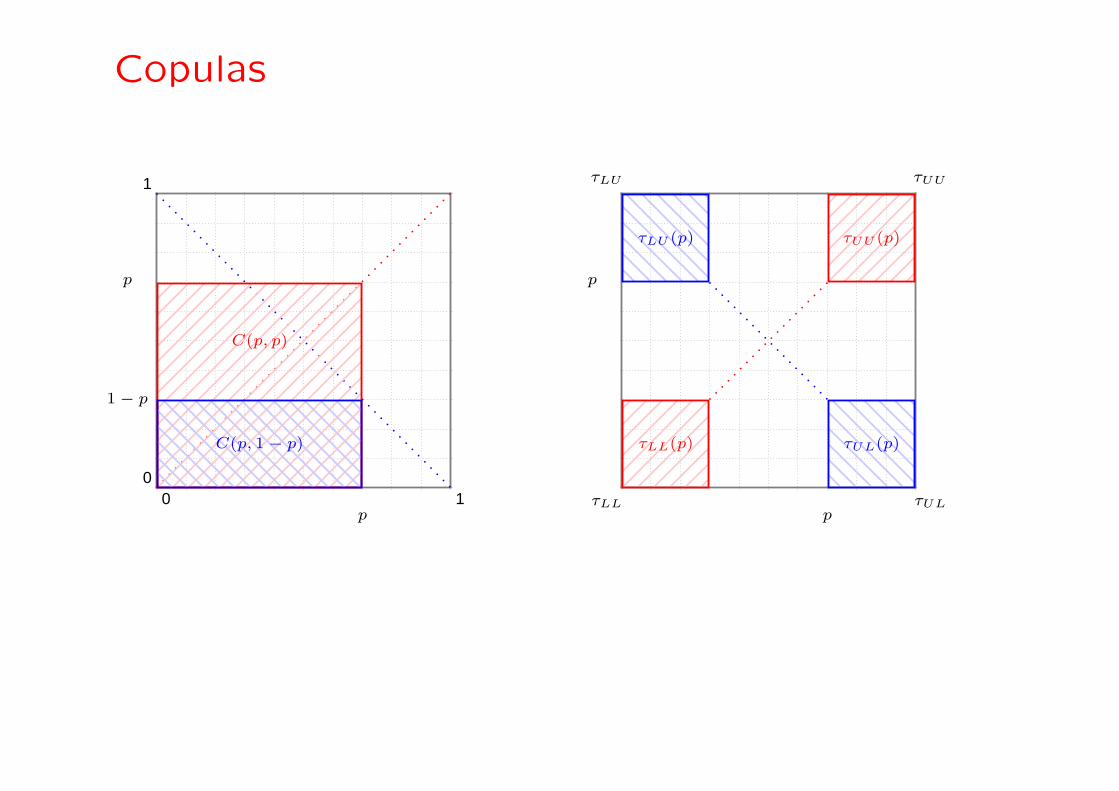
• Restricted information on copula: diagonal C(p, p) and

anti-diagonal C(p,1 − p). Note: C(12, 1

2) is the probability

that both variables are simultaneously below their medians

• Tail dependence:

τUU(p) =1 − 2p + C(p, p)

1 − p, etc.

• Relative difference with respect to independence or to

Gaussian:

C(p, p) − p2

p(1 − p)= τUU(p)+τLL(1−p)−1, or

C(p, p) − CG(p, p)

p(1 − p)

Copulas

0 10

1

C(p, p)

C(p, 1 − p)

p

p

1 − p

τUU (p)

p

p

τLL(p)

τLU (p)

τUL(p)

τLL

τLU

τUL

τUU

Student Copulas

• Intuition: r1 = σǫ1, r2 = σǫ2 with:

– ǫ1,2 bivariate Gaussian with correlation ρ

– σ is a common random volatility with distribution

P(σ) = N e−σ20/σ2

/σ1+ν

• The monovariate distributions of r1,2 are Student with a

power law tail exponent ν (∈ [3,5] for daily data)

• The multivariate Student is a model of correlated Gaussian

variables with a common random volatility:

ri = σǫi ρij = cov(ǫi, ǫj)

Student Copulas

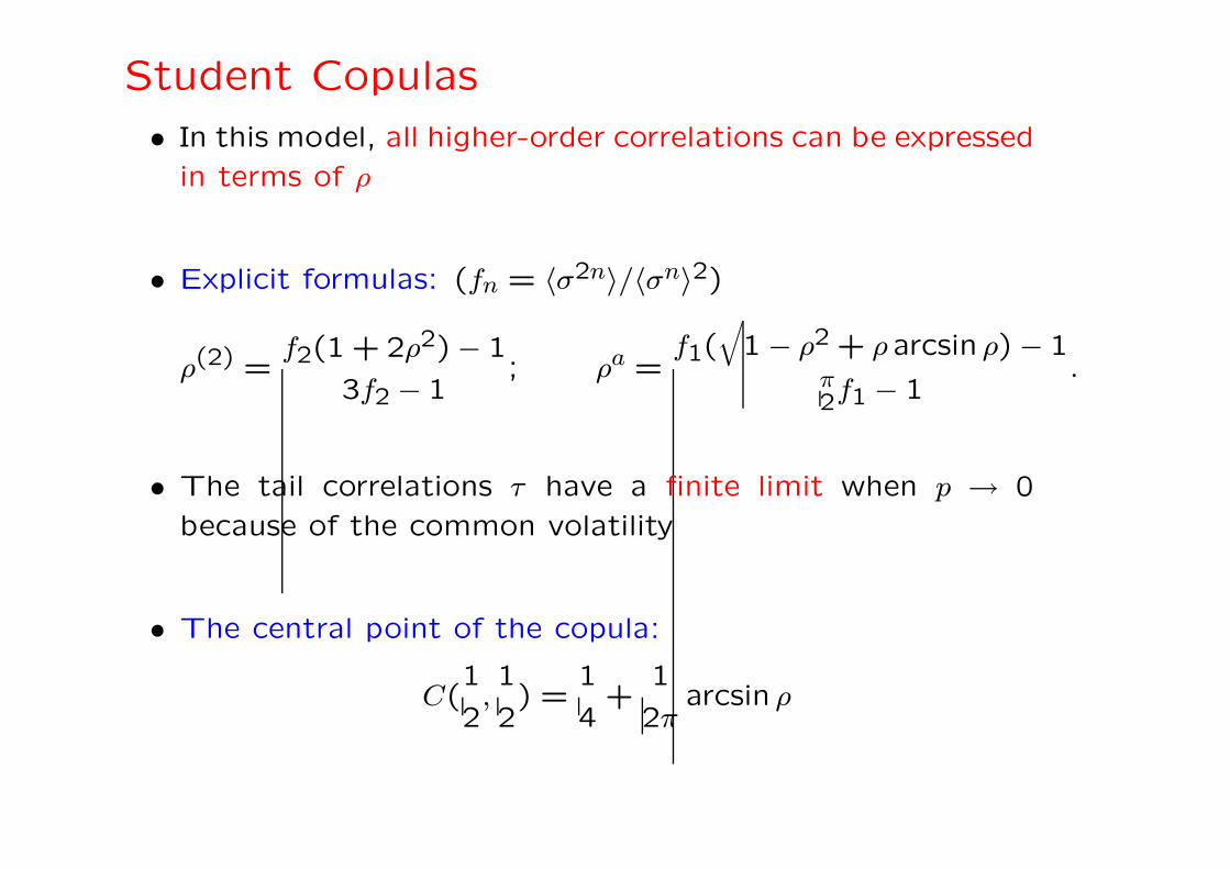
• In this model, all higher-order correlations can be expressed

in terms of ρ

• Explicit formulas: (fn = 〈σ2n〉/〈σn〉2)

ρ(2) =f2(1 + 2ρ2) − 1

3f2 − 1; ρa =

f1(√

1 − ρ2 + ρarcsin ρ) − 1π2f1 − 1

.

• The tail correlations τ have a finite limit when p → 0

because of the common volatility

• The central point of the copula:

C(1

2,1

2) =

1

4+

1

2πarcsin ρ

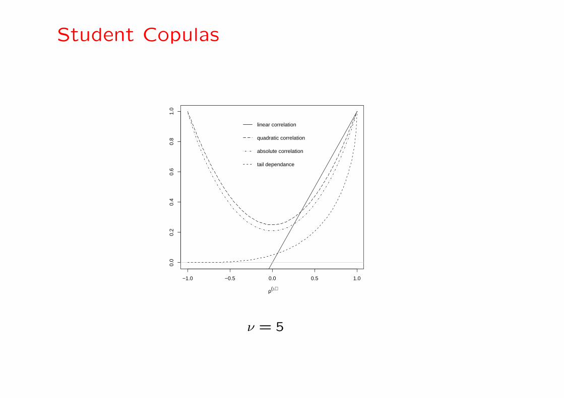
Student Copulas

−1.0 −0.5 0.0 0.5 1.0

0.0

0.2

0.4

0.6

0.8

1.0

ρ(1)

linear correlation

quadratic correlation

absolute correlation

tail dependance

ν = 5

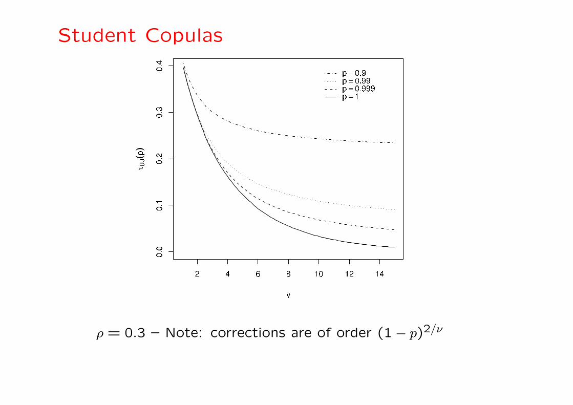
Student Copulas

ρ = 0.3 – Note: corrections are of order (1 − p)2/ν

Elliptic Copulas

• A straight-forward generalisation: elliptic copulas

r1 = σǫ1, r2 = σǫ2, P(σ) arbitrary

• The above formulas remain valid for arbitrary P(σ) in par-

ticular:

C(1

2,1

2) =

1

4+

1

2πarcsin ρ

• The tail correlations τ have a finite limit whenever P(σ)

decays as a power-law

• A relevant example: the log-normal model σ = σ0eξ, ξ =

N(0, λ2) – very similar to Student with ν ∼ λ−2 ∗

∗Although the true asymptotic value of τ(p = 0) is zero.

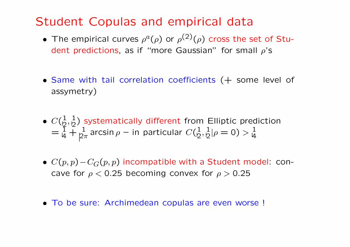
Student Copulas and empirical data

• The empirical curves ρa(ρ) or ρ(2)(ρ) cross the set of Stu-

dent predictions, as if “more Gaussian” for small ρ’s

• Same with tail correlation coefficients (+ some level of

assymetry)

• C(12, 1

2) systematically different from Elliptic prediction

= 14 + 1

2π arcsin ρ – in particular C(12, 1

2|ρ = 0) > 14

• C(p, p)−CG(p, p) incompatible with a Student model: con-

cave for ρ < 0.25 becoming convex for ρ > 0.25

• To be sure: Archimedean copulas are even worse !

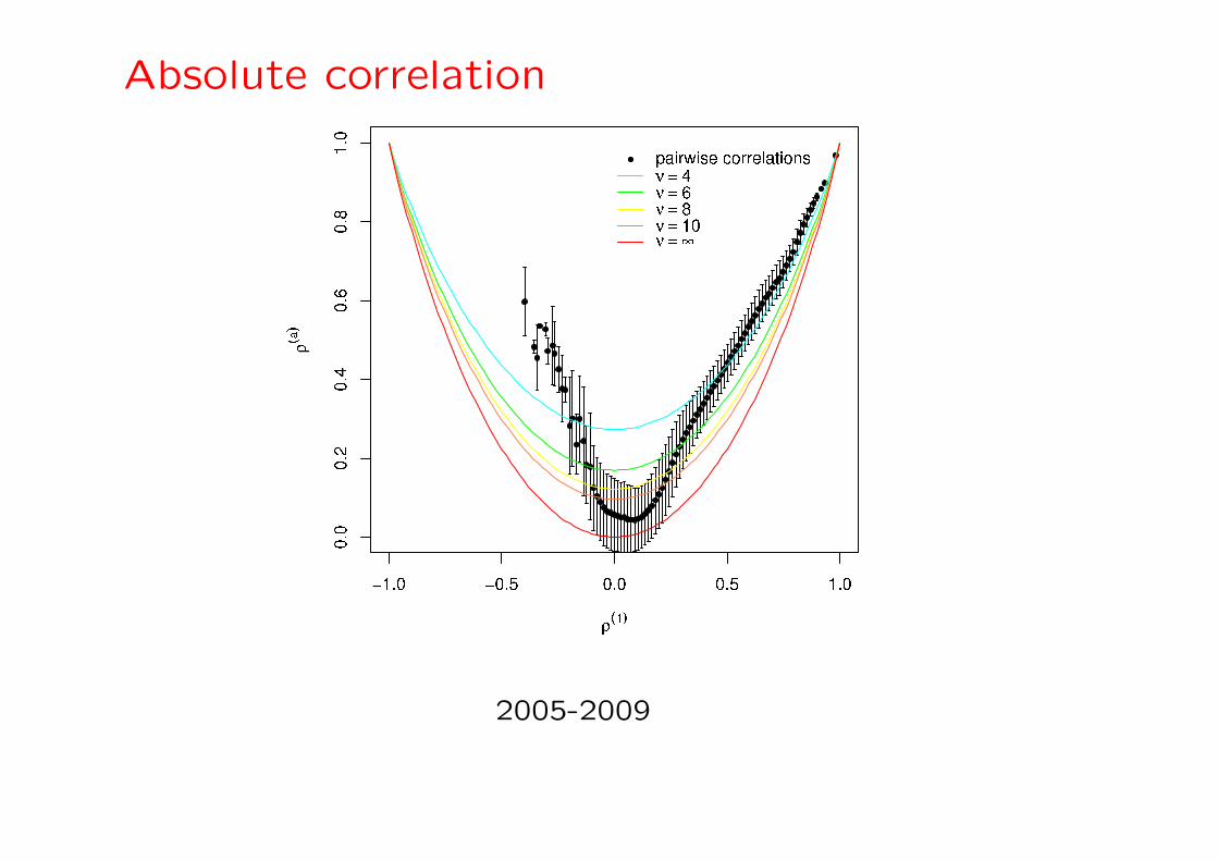
Absolute correlation

2005-2009

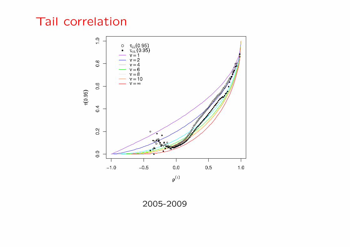
Tail correlation

2005-2009

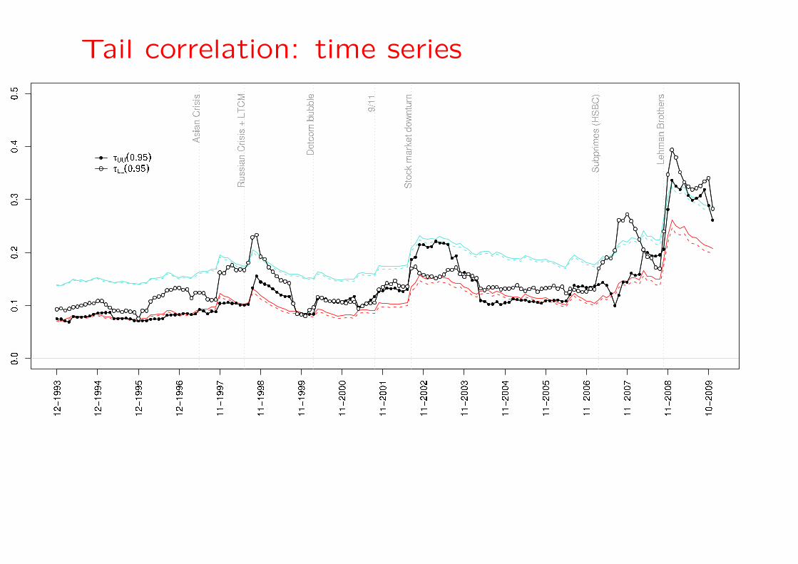
Tail correlation: time series

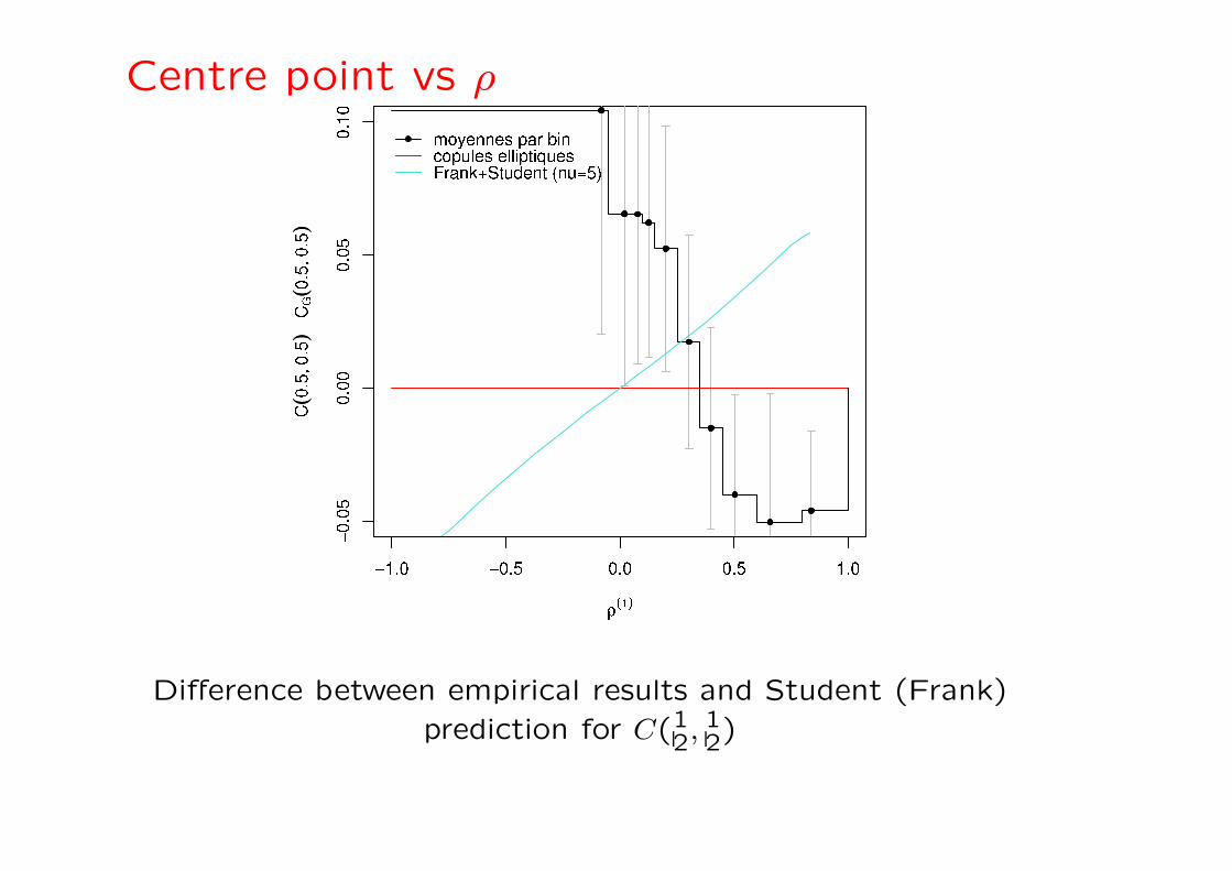
Centre point vs ρ

Difference between empirical results and Student (Frank)

prediction for C(12, 1

2)

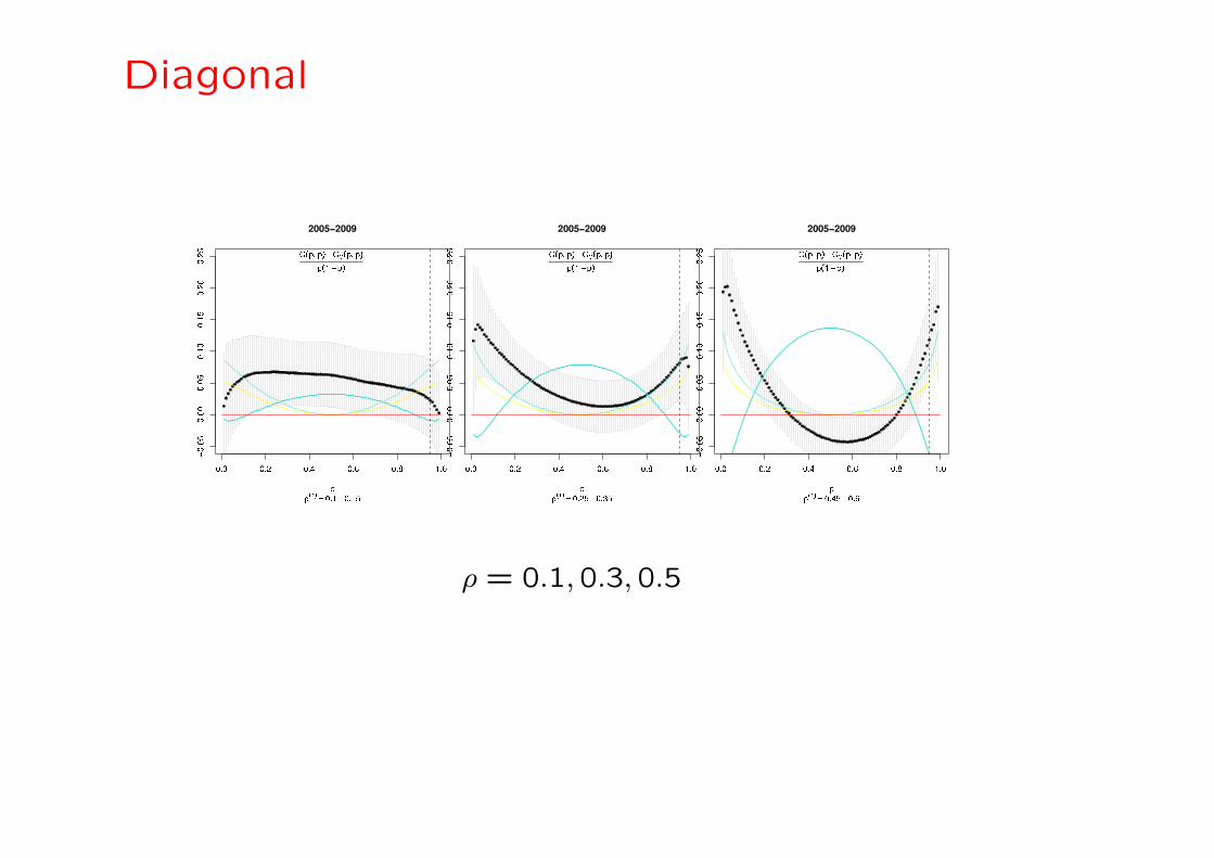
Diagonal

ρ = 0.1,0.3,0.5

Student Copulas: Conclusion

• Student (or even elliptic) copulas are not sufficient to de-

scribe the multivariate distribution of stocks!

• Obvious intuitive reason: one expects more than one volatil-

ity factor to affect stocks

• How to describe an entangled correlation between returns

and volatilities?

• In particular, any model such that ri = σiǫi with correlated

random σ’s leads to C(12, 1

2) ≡ 14 for ρ = 0!

Constructing a realistic copula model

• How do we go about now (for stocks) ?

– a) stocks are sensitive to “factors”

– b) factors are hierarchical, in the sense that the vol

of the market influences that of sectors, which in turn

influence that of more idiosyncratic factors

• Empirical fact: within a one-factor model,

ri = βiε0 + εi

volatility of residuals increases with that of the market ε0

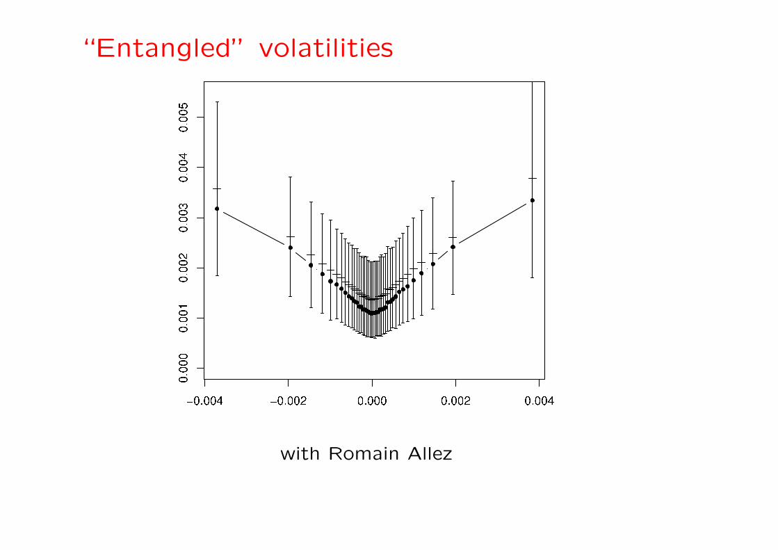
“Entangled” volatilities

with Romain Allez

Constructing a realistic copula model

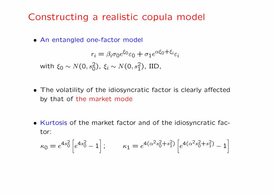
• An entangled one-factor model

ri = βiσ0eξ0ε0 + σ1eαξ0+ξiεi

with ξ0 ∼ N(0, s20), ξi ∼ N(0, s21), IID,

• The volatility of the idiosyncratic factor is clearly affected

by that of the market mode

• Kurtosis of the market factor and of the idiosyncratic fac-

tor:

κ0 = e4s20

[

e4s20 − 1

]

; κ1 = e4(α2s20+s21)[

e4(α2s20+s21) − 1

]

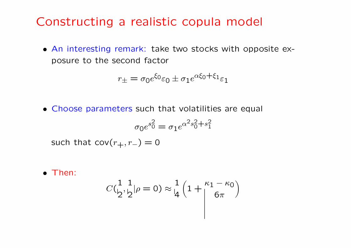
Constructing a realistic copula model

• An interesting remark: take two stocks with opposite ex-

posure to the second factor

r± = σ0eξ0ε0 ± σ1eαξ0+ξ1ε1

• Choose parameters such that volatilities are equal

σ0es20 = σ1eα2s20+s21

such that cov(r+, r−) = 0

• Then:

C(1

2,1

2|ρ = 0) ≈

1

4

(

1 +κ1 − κ0

6π

)

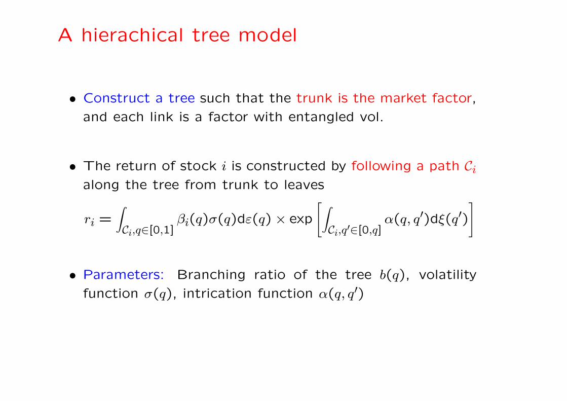
A hierachical tree model

• Construct a tree such that the trunk is the market factor,

and each link is a factor with entangled vol.

• The return of stock i is constructed by following a path Ci

along the tree from trunk to leaves

ri =∫

Ci,q∈[0,1]βi(q)σ(q)dε(q) × exp

[

∫

Ci,q′∈[0,q]α(q, q′)dξ(q′)

]

• Parameters: Branching ratio of the tree b(q), volatility

function σ(q), intrication function α(q, q′)

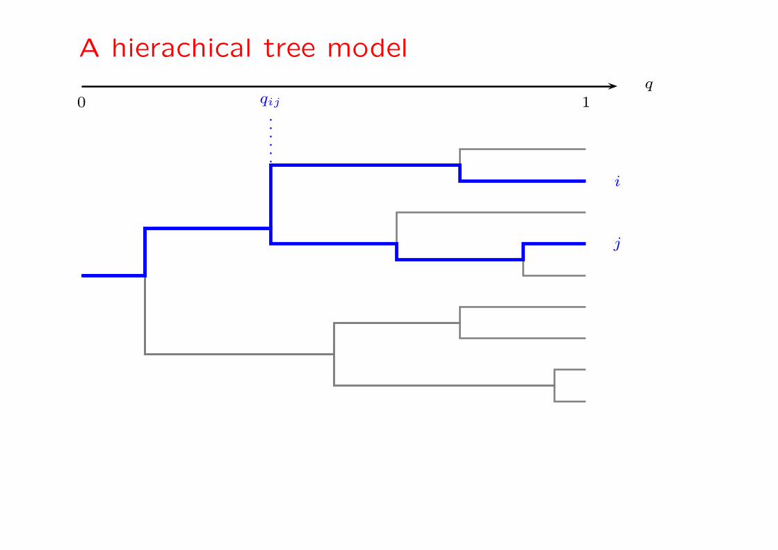
A hierachical tree model

i

j

qij

q

0 1

A hierachical tree model

• Calibration on data: work in progress...

• Find simple, systematic ways to calibrate such a huge

model ⇒ stability of Rij??

• Preliminary simulation results for reasonable choices: the

model is able to reproduce all the empirical facts reported

above, including C(1/2,1/2) > 1/4 and the change of con-

cavity of

C(p, p) − CG(p, p)

p(1 − p)

as ρ increases

Self-copulas

• One can also define the copula between a variable and

itself, lagged:

Cτ(u, v) = P

[

P<(Xt) ≤ u and P<,j(Xt+τ) ≤ v]

• Example: log-normal copula

Xt = eωtξt

with correlations between ξ’s (linear), ω’s (vol) and ωξ

(leverage)

• In the limit of weak correlations:

Ct(u, v) − uv ≈ ρR(u, v) + αA(u, v) − βB(u, v)

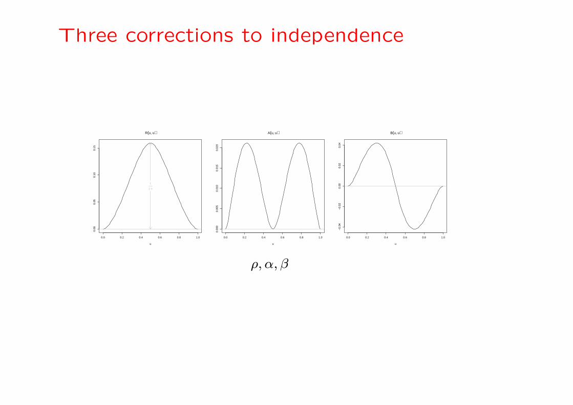
Three corrections to independence

0.0 0.2 0.4 0.6 0.8 1.0

0.00

0.05

0.10

0.15

R(u, u)

u

1

2 π

0.0 0.2 0.4 0.6 0.8 1.0

0.00

00.

005

0.01

00.

015

0.02

0

A(u, u)

u

0.0 0.2 0.4 0.6 0.8 1.0

−0.

04−

0.02

0.00

0.02

0.04

B(u, u)

u

ρ, α, β

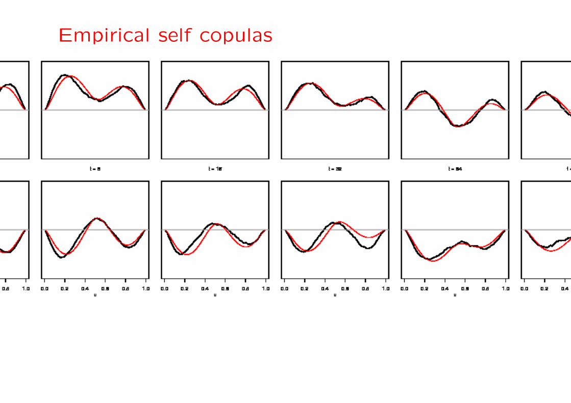
Empirical self copulas

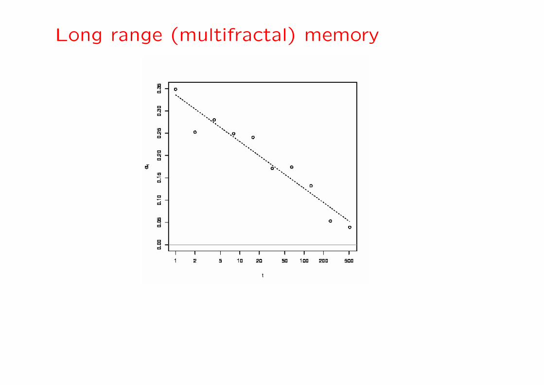
Long range (multifractal) memory

Self-copulas

• A direct application: GoF tests (Kolmogorov-Smirnov/Cramer-

von Mises) for dependent variables

• The relevant quantity is∑

t (Ct(u, v) + C−t(u, v) − 2uv)

• The test is dependent on the self-copula

• ⇒ Significant decrease of the effective number of indepen-

dent variables

Conclusion – Open problems

• GoF tests for two-dimensional copulas: max of “Brownian

sheets” (some progress with Remy)

• Structural model: requires analytical progress (possible

thanks to the tree structure) and numerical simulations

• Extension to account for U/L asymmetry

• Extension to describe defaults and time to defaults – move

away from silly models and introduce some underlying

structure