copyright © 2006, brigham s. anderson machine learning and the axioms of probability brigham s....
Post on 21-Dec-2015
248 views
TRANSCRIPT

Copyright © 2006, Brigham S. Anderson
Machine Learning and the Axioms of
Probability
Brigham S. Andersonwww.cs.cmu.edu/~brigham
School of Computer Science
Carnegie Mellon University

2
Copyright © 2006, Brigham S. Anderson
Probability
• The world is a very uncertain place
• 30 years of Artificial Intelligence and Database research danced around this fact
• And then a few AI researchers decided to use some ideas from the eighteenth century

3
Copyright © 2006, Brigham S. Anderson
What we’re going to do
• We will review the fundamentals of probability.
• It’s really going to be worth it
• You’ll see examples of probabilistic analytics in action: • Inference, • Anomaly detection, and • Bayes Classifiers

4
Copyright © 2006, Brigham S. Anderson
Discrete Random Variables
• A is a Boolean-valued random variable if A denotes an event, and there is some degree of uncertainty as to whether A occurs.
• Examples• A = The US president in 2023 will be male• A = You wake up tomorrow with a headache• A = You have influenza

5
Copyright © 2006, Brigham S. Anderson
Probabilities
• We write P(A) as “the probability that A is true”
• We could at this point spend 2 hours on the philosophy of this.
• We’ll spend slightly less...

6
Copyright © 2006, Brigham S. Anderson
Sample Space
Definition 1.The set, S, of all possible outcomes of a particular experiment is called the sample space for the experiment
The elements of the sample space are called outcomes.

7
Copyright © 2006, Brigham S. Anderson
Sample Spaces
Sample space of a coin flip:
S = {H, T}
H
T

8
Copyright © 2006, Brigham S. Anderson
Sample Spaces
Sample space of a die roll:
S = {1, 2, 3, 4, 5, 6}

9
Copyright © 2006, Brigham S. Anderson
Sample Spaces
Sample space of three die rolls?
S = {111,112,113,…,
…,664,665,666}

10
Copyright © 2006, Brigham S. Anderson
Sample SpacesSample space of a single draw from a
deck of cards:
S={As,Ac,Ah,Ad,2s,2c,2h,…
…,Ks,Kc,Kd,Kh}
11
Copyright © 2006, Brigham S. Anderson
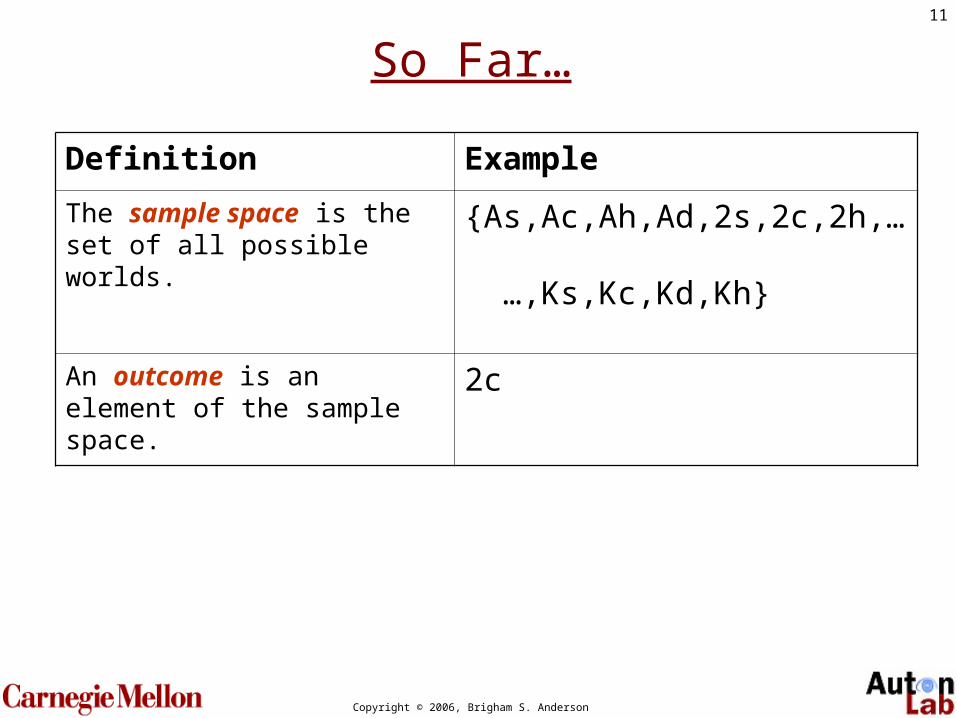
So Far…
Definition ExampleThe sample space is the set of all possible worlds.
{As,Ac,Ah,Ad,2s,2c,2h,… …,Ks,Kc,Kd,Kh}
An outcome is an element of the sample space.
2c

12
Copyright © 2006, Brigham S. Anderson
Events
Definition 2.An event is any subset of S (including S itself)
13
Copyright © 2006, Brigham S. Anderson
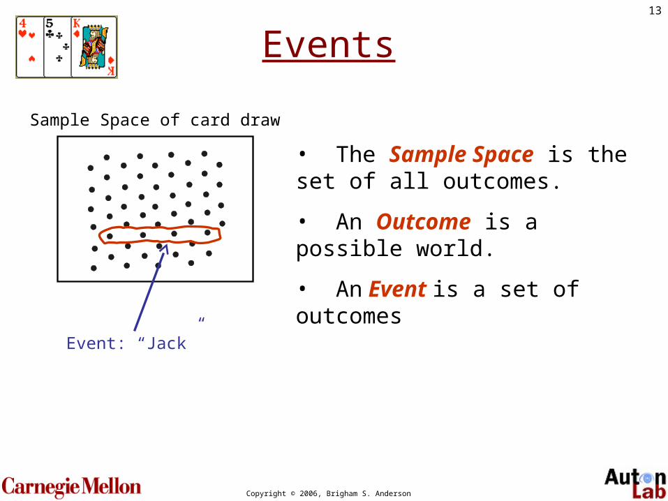
Events
Event: “Jack”
Sample Space of card draw
• The Sample Space is the set of all outcomes.
• An Outcome is a possible world.
• An Event is a set of outcomes

14
Copyright © 2006, Brigham S. Anderson
Events
Event: “Hearts”
Sample Space of card draw
• The Sample Space is the set of all outcomes.
• An Outcome is a possible world.
• An Event is a set of outcomes

15
Copyright © 2006, Brigham S. Anderson
Events
Event: “Red and Face”
Sample Space of card draw
• The Sample Space is the set of all outcomes.
• An Outcome is a possible world.
• An Event is a set of outcomes
16
Copyright © 2006, Brigham S. Anderson
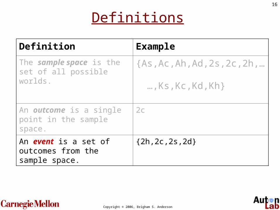
Definitions
Definition Example
The sample space is the set of all possible worlds.
{As,Ac,Ah,Ad,2s,2c,2h,… …,Ks,Kc,Kd,Kh}
An outcome is a single point in the sample space.
2c
An event is a set of outcomes from the sample space.
{2h,2c,2s,2d}

17
Copyright © 2006, Brigham S. Anderson
Events
Definition 3.Two events A and B are mutually exclusive if A^B=Ø.
Definition 4.If A1, A2, … are mutually exclusive and A1 A2 … = S, then the collection A1, A2, … forms a partition of S.
clubs
hearts spades
diamonds

18
Copyright © 2006, Brigham S. Anderson
Probability
Definition 5.Given a sample space S, a probability function is a function that maps each event in S to a real number, and satisfies
• P(A) ≥ 0 for any event A in S• P(S) = 1• For any number of mutually exclusive events A1, A2, A3 …, we have P(A1 A2 A3 …) = P(A1) + P(A2) + P(A3) +…
** This definition of the domain of this function is
not 100% sufficient, but it’s close enough for our purposes… (I’m sparing you Borel Fields)

19
Copyright © 2006, Brigham S. Anderson
Definitions
Definition Example
The sample space is the set of all possible worlds.
{As,Ac,Ah,Ad,2s,2c,2h,… …,Ks,Kc,Kd,Kh}
An outcome is a single point in the sample space.
4c
An event is a set of one or more outcomes
Card is “Red”
P(E) maps event E to a real number and satisfies the axioms of probability
P(Red) = 0.50P(Black) = 0.50

20
Copyright © 2006, Brigham S. Anderson
A
~A
Misconception
• The relative area of the events determines their probability
• …in a Venn diagram it does, but not in general.• However, the “area equals probability” rule is guaranteed
to result in axiom-satisfying probability functions.
We often assume, for example, that the probability of “heads” is equal to
“tails” in absence of other information…
But this is totally outside the axioms!

21
Copyright © 2006, Brigham S. Anderson
Creating a Valid P()
• One convenient way to create an axiom-satisfying probability function:
1. Assign a probability to each outcome in S
2. Make sure they sum to one
3. Declare that P(A) equals the sum of outcomes in event A

22
Copyright © 2006, Brigham S. Anderson
Everyday Example
Assume you are a doctor.
This is the sample space of “patients you might see on any given day”.
Non-smoker, female, diabetic, headache, good insurance, etc…
Smoker, male, herniated disk, back pain, mildly schizophrenic, delinquent medical bills, etc…
Outcomes

23
Copyright © 2006, Brigham S. Anderson
Everyday Example
Number of elements in the “patient space”:
100 jillion
Are these patients equally likely to occur?
Again, generally not. Let’s assume for the moment that they are, though.
…which roughly means “area equals probability”
24
Copyright © 2006, Brigham S. Anderson
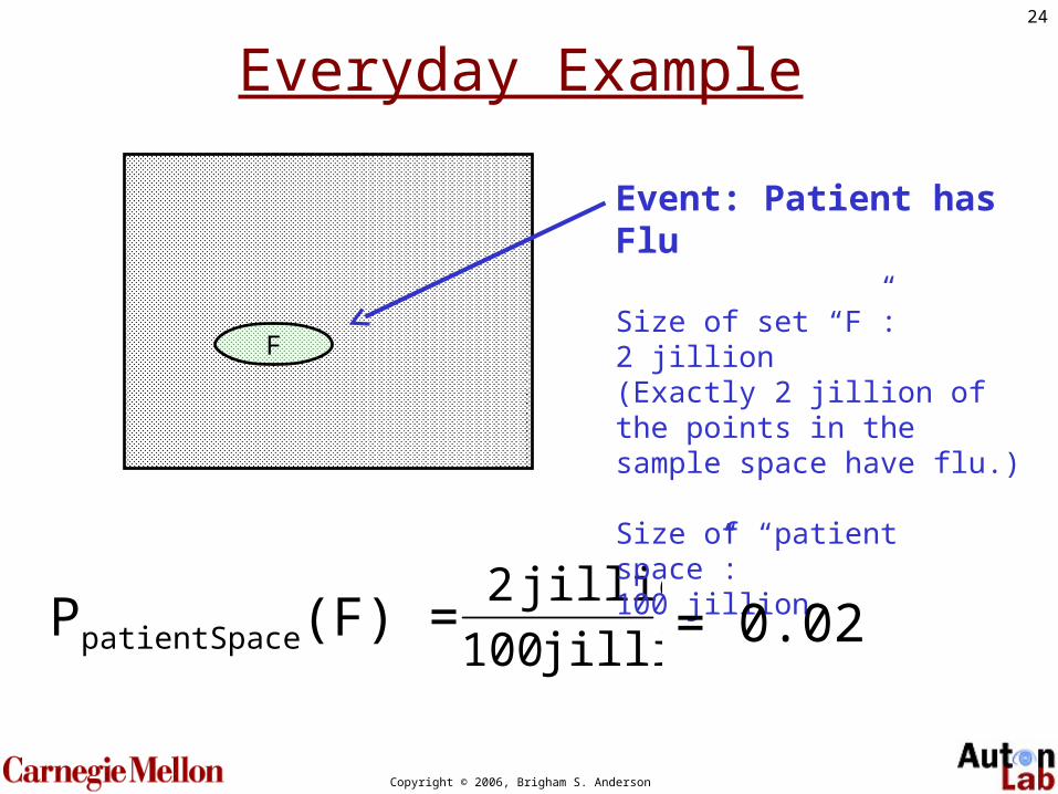
Everyday Example
jillion100
jillion2
F
Event: Patient has Flu
Size of set “F”:2 jillion(Exactly 2 jillion of the points in the sample space have flu.)
Size of “patient space”:100 jillion
= 0.02PpatientSpace(F) =

25
Copyright © 2006, Brigham S. Anderson
Everyday Example
jillion100
jillion2
F
= 0.02PpatientSpace(F) =
From now on, the subscript on P() willbe omitted…

26
Copyright © 2006, Brigham S. Anderson
These Axioms are Not to be Trifled With
• There have been attempts to do different methodologies for uncertainty
• Fuzzy Logic• Three-valued logic• Dempster-Shafer• Non-monotonic reasoning
• But the axioms of probability are the only system with this property:
If you gamble using them you can’t be unfairly exploited by an opponent using some other system [di Finetti 1931]

27
Copyright © 2006, Brigham S. Anderson
Theorems from the AxiomsAxioms• P(A) ≥ 0 for any event A in S• P(S) = 1• For any number of mutually exclusive events A1, A2, A3 …, we have P(A1 A2 A3 …) = P(A1) + P(A2) + P(A3) +…
Theorem.If P is a probability function and A is an event in S, thenP(~A) = 1 – P(A)
Proof:(1) Since A and ~A partition S, P(A ~A) = P(S) = 1
(2) Since A and ~A are disjoint, P(A ~A) = P(A) + P(~A)
Combining (1) and (2) gives the result

28
Copyright © 2006, Brigham S. Anderson
Multivalued Random Variables
• Suppose A can take on more than 2 values
• A is a random variable with arity k if it can take on exactly one value out of {A1,A2, ... Ak}, and
• The events {A1,A2,…,Ak} partition S, so
jiAAP ji if 0),(
1)...( 21 kAAAP

29
Copyright © 2006, Brigham S. Anderson
Elementary Probability in Pictures
P(~A) + P(A) = 1
A
~A

30
Copyright © 2006, Brigham S. Anderson
Elementary Probability in Pictures
P(B) = P(B, A) + P(B, ~A)
A
~A
B
31
Copyright © 2006, Brigham S. Anderson
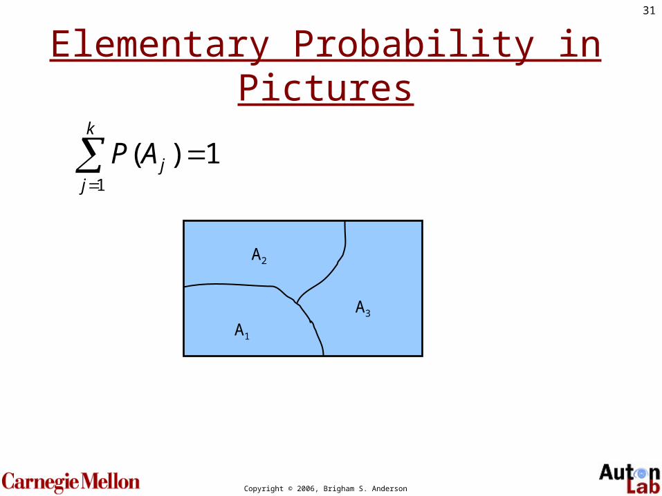
Elementary Probability in Pictures
1)(1
k
jjAP
A1
A2
A3

32
Copyright © 2006, Brigham S. Anderson
Elementary Probability in Pictures
),()(1
k
jjABPBP
A1
A2
A3
B
Useful!
33
Copyright © 2006, Brigham S. Anderson
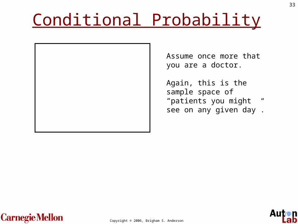
Conditional Probability
Assume once more that you are a doctor.
Again, this is the sample space of “patients you might see on any given day”.

34
Copyright © 2006, Brigham S. Anderson
Conditional Probability
F
Event: Flu
P(F) = 0.02
35
Copyright © 2006, Brigham S. Anderson
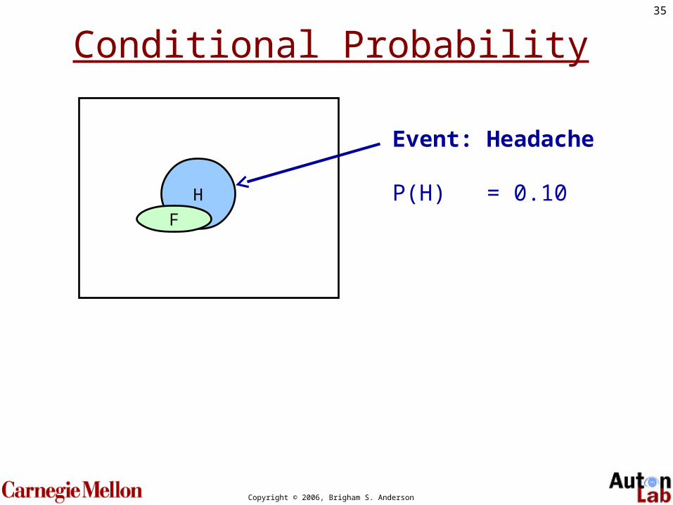
Conditional Probability
Event: Headache
P(H) = 0.10H
F
36
Copyright © 2006, Brigham S. Anderson
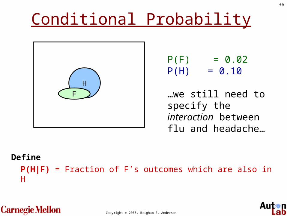
Conditional Probability
P(F) = 0.02P(H) = 0.10
…we still need to specify the interaction between flu and headache…
Define
P(H|F) = Fraction of F’s outcomes which are also in H
H
F

37
Copyright © 2006, Brigham S. Anderson
H
Conditional Probability
F
P(F) = 0.02P(H) = 0.10P(H|F) = 0.50
0.01 0.01
0.89
0.09
H = “headache”F = “flu”

38
Copyright © 2006, Brigham S. Anderson
Conditional Probability
H = “headache”F = “flu”
P(H|F) = Fraction of flu worlds in which patient has a headache
= #worlds with flu and headache ------------------------------------ #worlds with flu
= Size of “H and F” region ------------------------------ Size of “F” region
= P(H, F) ---------- P(F)
F
0.01 0.01
0.89
0.09H

39
Copyright © 2006, Brigham S. Anderson
Conditional Probability
Definition.If A and B are events in S, and P(B) > 0, then the conditional probability of A given B, written P(A|B), is
)(
),()|(
BP
BAPBAP
The Chain RuleA simple rearrangement of the above equation yields
)()|(),( BPBAPBAP Main BayesNet concept!

40
Copyright © 2006, Brigham S. Anderson
Probabilistic Inference
H = “Have a headache”F = “Coming down with Flu”
P(H) = 0.10P(F) = 0.02P(H|F) = 0.50
One day you wake up with a headache. You think: “Drat! 50% of flus are associated with headaches so I must have a 50-50 chance of coming down with flu”
Is this reasoning good?
H
F

41
Copyright © 2006, Brigham S. Anderson
Probabilistic Inference
)(
),()|(
HP
HFPHFP
)(
)()|(
HP
FPFHP
H
F
10.01.0
)02.0()50.0(
H = “Have a headache”F = “Coming down with Flu”
P(H) = 0.10P(F) = 0.02P(H|F) = 0.50

42
Copyright © 2006, Brigham S. Anderson
What we just did…
P(A,B) P(A|B) P(B)
P(B|A) = ----------- = ---------------
P(A) P(A)
This is Bayes Rule
Bayes, Thomas (1763) An essay towards solving a problem in the doctrine of chances. Philosophical Transactions of the Royal Society of London, 53:370-418

43
Copyright © 2006, Brigham S. Anderson
More General Forms of Bayes Rule
)(~)|~()()|(
)()|()|(
APABPAPABP
APABPBAP
),(
),(),|(),|(
CBP
CAPCABPCBAP

44
Copyright © 2006, Brigham S. Anderson
More General Forms of Bayes Rule
An
kkk
iii
APABP
APABPBAP
1
)()|(
)()|()|(

45
Copyright © 2006, Brigham S. Anderson
Independence
Definition.Two events, A and B, are statistically independent if
)()(),( BPAPBAP
Which is equivalent to
)()|( APBAP
Important forBayes Nets
46
Copyright © 2006, Brigham S. Anderson
Representing P(A,B,C)
• How can we represent the function P(A)?• P(A,B)?• P(A,B,C)?

47
Copyright © 2006, Brigham S. Anderson
Recipe for making a joint distribution of M variables:
1. Make a truth table listing all combinations of values of your variables (if there are M boolean variables then the table will have 2M rows).
2. For each combination of values, say how probable it is.
3. If you subscribe to the axioms of probability, those numbers must sum to 1.
A B C Prob
0 0 0 0.30
0 0 1 0.05
0 1 0 0.10
0 1 1 0.05
1 0 0 0.05
1 0 1 0.10
1 1 0 0.25
1 1 1 0.10
Example: P(A, B, C)
A
B
C0.050.25
0.10 0.050.05
0.10
0.100.30
The Joint Probability Table

48
Copyright © 2006, Brigham S. Anderson
Using the Joint
One you have the JPT you can ask for the probability of any logical expression
E
PEP matching rows
)row()(
…what is P(Poor,Male)?

49
Copyright © 2006, Brigham S. Anderson
Using the Joint
P(Poor, Male) = 0.4654 E
PEP matching rows
)row()(
…what is P(Poor)?

50
Copyright © 2006, Brigham S. Anderson
Using the Joint
P(Poor) = 0.7604 E
PEP matching rows
)row()(
…what is P(Poor|Male)?

51
Copyright © 2006, Brigham S. Anderson
Inference with the
Joint
2
2 1
matching rows
and matching rows
2
2121 )row(
)row(
)(
),()|(
E
EE
P
P
EP
EEPEEP

52
Copyright © 2006, Brigham S. Anderson
Inference with the
Joint
2
2 1
matching rows
and matching rows
2
2121 )row(
)row(
)(
),()|(
E
EE
P
P
EP
EEPEEP
P(Male | Poor) = 0.4654 / 0.7604 = 0.612

53
Copyright © 2006, Brigham S. Anderson
Inference is a big deal• I’ve got this evidence. What’s the chance that this
conclusion is true?• I’ve got a sore neck: how likely am I to have meningitis?• I see my lights are out and it’s 9pm. What’s the chance my spouse
is already asleep?
• There’s a thriving set of industries growing based around Bayesian Inference. Highlights are: Medicine, Pharma, Help Desk Support, Engine Fault Diagnosis

54
Copyright © 2006, Brigham S. Anderson
Where do Joint Distributions come from?
• Idea One: Expert Humans• Idea Two: Simpler probabilistic facts and some algebraExample: Suppose you knew
P(A) = 0.5P(B|A) = 0.2P(B|~A) = 0.1
P(C|A,B) = 0.1P(C|A,~B) = 0.8P(C|~A,B) = 0.3P(C|~A,~B) = 0.1
Then you can automatically compute the JPT using the chain rule
P(A,B,C) = P(A) P(B|A) P(C|A,B)
Bayes Nets are a systematic way to do this.

55
Copyright © 2006, Brigham S. Anderson
Where do Joint Distributions come from?
• Idea Three: Learn them from data!
Prepare to witness an impressive learning algorithm….

56
Copyright © 2006, Brigham S. Anderson
Learning a JPT
Build a Joint Probability table for your attributes in which the probabilities are unspecified
Then fill in each row with
records ofnumber total
row matching records)row(ˆ P
A B C Prob
0 0 0 ?
0 0 1 ?
0 1 0 ?
0 1 1 ?
1 0 0 ?
1 0 1 ?
1 1 0 ?
1 1 1 ?
A B C Prob
0 0 0 0.30
0 0 1 0.05
0 1 0 0.10
0 1 1 0.05
1 0 0 0.05
1 0 1 0.10
1 1 0 0.25
1 1 1 0.10
Fraction of all records in whichA and B are True but C is False
57
Copyright © 2006, Brigham S. Anderson
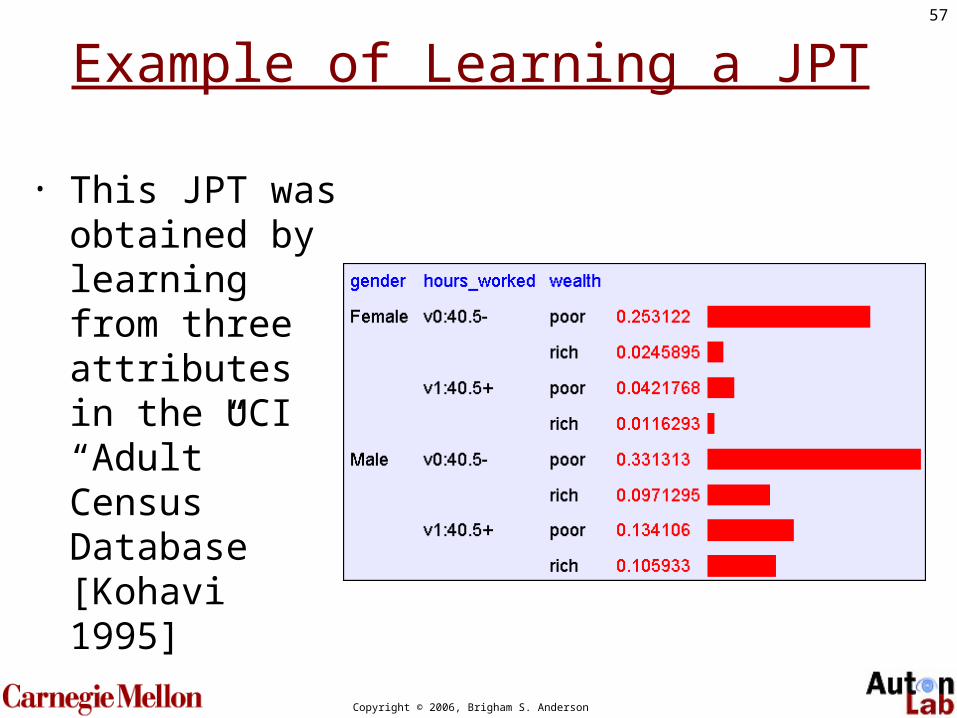
Example of Learning a JPT
• This JPT was obtained by learning from three attributes in the UCI “Adult” Census Database [Kohavi 1995]
58
Copyright © 2006, Brigham S. Anderson
Where are we?
• We have recalled the fundamentals of probability
• We have become content with what JPTs are and how to use them
• And we even know how to learn JPTs from data.

59
Copyright © 2006, Brigham S. Anderson
Density Estimation
• Our Joint Probability Table (JPT) learner is our first example of something called Density Estimation
• A Density Estimator learns a mapping from a set of attributes to a Probability
DensityEstimator
ProbabilityInput
Attributes

60
Copyright © 2006, Brigham S. Anderson
• Given a record x, a density estimator M can tell you how likely the record is:
• Given a dataset with R records, a density estimator can tell you how likely the dataset is:(Under the assumption that all records were independently generated
from the probability function)
Evaluating a density estimator
R
kkR |MP|MP|MP
121 )(ˆ),,(ˆ)dataset(ˆ xxxx
)(ˆ |MP x
61
Copyright © 2006, Brigham S. Anderson
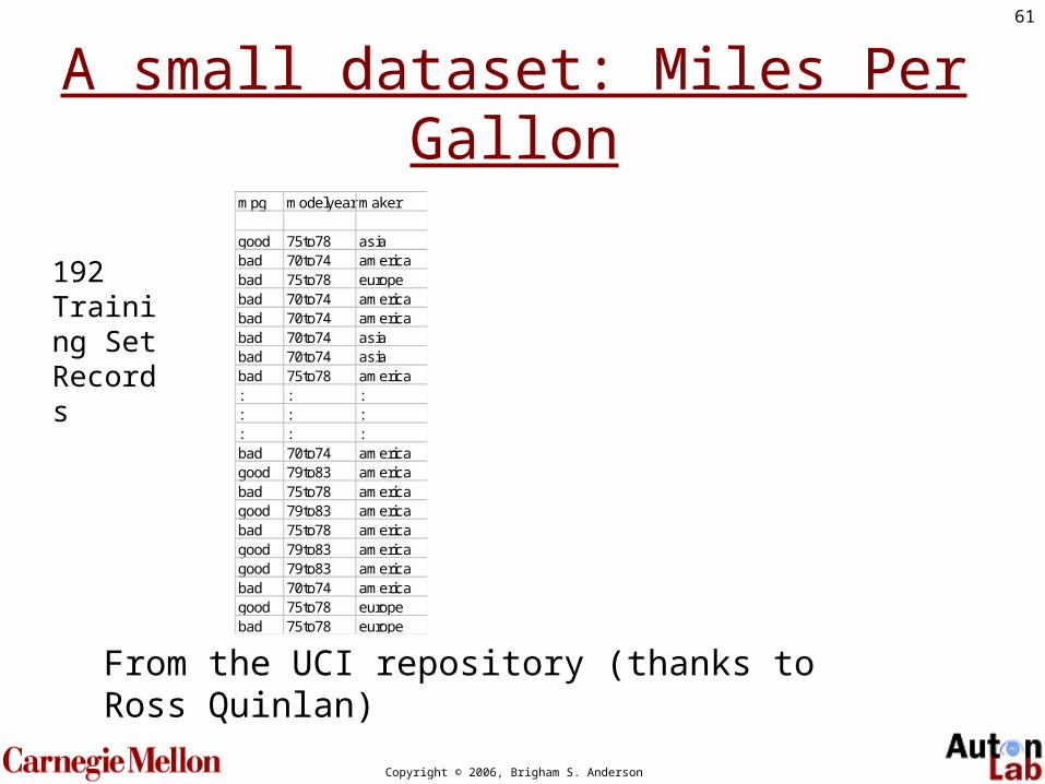
A small dataset: Miles Per Gallon
From the UCI repository (thanks to Ross Quinlan)
192 Training Set Records
mpg modelyear maker
good 75to78 asiabad 70to74 americabad 75to78 europebad 70to74 americabad 70to74 americabad 70to74 asiabad 70to74 asiabad 75to78 america: : :: : :: : :bad 70to74 americagood 79to83 americabad 75to78 americagood 79to83 americabad 75to78 americagood 79to83 americagood 79to83 americabad 70to74 americagood 75to78 europebad 75to78 europe

62
Copyright © 2006, Brigham S. Anderson
A small dataset: Miles Per Gallon
192 Training Set Records
mpg modelyear maker
good 75to78 asiabad 70to74 americabad 75to78 europebad 70to74 americabad 70to74 americabad 70to74 asiabad 70to74 asiabad 75to78 america: : :: : :: : :bad 70to74 americagood 79to83 americabad 75to78 americagood 79to83 americabad 75to78 americagood 79to83 americagood 79to83 americabad 70to74 americagood 75to78 europebad 75to78 europe

63
Copyright © 2006, Brigham S. Anderson
A small dataset: Miles Per Gallon
192 Training Set Records
mpg modelyear maker
good 75to78 asiabad 70to74 americabad 75to78 europebad 70to74 americabad 70to74 americabad 70to74 asiabad 70to74 asiabad 75to78 america: : :: : :: : :bad 70to74 americagood 79to83 americabad 75to78 americagood 79to83 americabad 75to78 americagood 79to83 americagood 79to83 americabad 70to74 americagood 75to78 europebad 75to78 europe
203-1
21
10 3.4
)(ˆ),,(ˆ)dataset(ˆ
R
kkR |MP|MP|MP xxxx
64
Copyright © 2006, Brigham S. Anderson
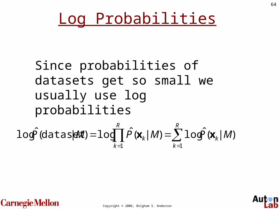
Log Probabilities
Since probabilities of datasets get so small we usually use log probabilities
R
kk
R
kk |MP|MP|MP
11
)(ˆlog)(ˆlog)dataset(ˆlog xx

65
Copyright © 2006, Brigham S. Anderson
A small dataset: Miles Per Gallon
192 Training Set Records
mpg modelyear maker
good 75to78 asiabad 70to74 americabad 75to78 europebad 70to74 americabad 70to74 americabad 70to74 asiabad 70to74 asiabad 75to78 america: : :: : :: : :bad 70to74 americagood 79to83 americabad 75to78 americagood 79to83 americabad 75to78 americagood 79to83 americagood 79to83 americabad 70to74 americagood 75to78 europebad 75to78 europe
466.19
)(ˆlog)(ˆlog)dataset(ˆlog11
R
kk
R
kk |MP|MP|MP xx

66
Copyright © 2006, Brigham S. Anderson
Summary: The Good News
The JPT allows us to learn P(X) from data.
• Can do inference: P(E1|E2)Automatic Doctor, Recommender, etc
• Can do anomaly detection spot suspicious / incorrect records
(e.g., credit card fraud)
• Can do Bayesian classificationPredict the class of a record
(e.g, predict cancerous/not-cancerous)

67
Copyright © 2006, Brigham S. Anderson
Summary: The Bad News
• Density estimation with JPTs is trivial, mindless and dangerous

68
Copyright © 2006, Brigham S. Anderson
Using a test set
An independent test set with 196 cars has a much worse log likelihood than it had on the training set
(actually it’s a billion quintillion quintillion quintillion quintillion times less likely)
….Density estimators can overfit. And the JPT estimator is the overfittiest of them all!

69
Copyright © 2006, Brigham S. Anderson
Overfitting Density Estimators
If this ever happens, it means there are certain combinations that we learn are “impossible”

70
Copyright © 2006, Brigham S. Anderson
Using a test set
The only reason that our test set didn’t score -infinity is that Andrew’s code is hard-wired to always predict a probability of at least one in 1020
We need Density Estimators that are less prone to overfitting

71
Copyright © 2006, Brigham S. Anderson
Is there a better way?
The problem with the JPT is that it just mirrors the training data.
In fact, it is just another way of storing the data: we could reconstruct the original dataset perfectly from it!
We need to represent the probability function with fewer parameters…

72
Copyright © 2006, Brigham S. Anderson
Aside:Bayes Nets

73
Copyright © 2006, Brigham S. Anderson
Bayes Nets• What are they?
• Bayesian nets are a framework for representing and analyzing models involving uncertainty
• What are they used for?• Intelligent decision aids, data fusion, 3-E feature recognition,
intelligent diagnostic aids, automated free text understanding, data mining
• How are they different from other knowledge representation and probabilistic analysis tools?• Uncertainty is handled in a mathematically rigorous yet efficient
and simple way

74
Copyright © 2006, Brigham S. Anderson
Bayes Net Concepts
1.Chain RuleP(A,B) = P(A) P(B|A)
2.Conditional IndependenceP(A|B,C) = P(A|B)

75
Copyright © 2006, Brigham S. Anderson
A Simple Bayes Net
• Let’s assume that we already have P(Mpg,Horse)
How would you rewrite this using the Chain rule?
0.480.12bad
0.040.36good
highlowP(good, low) = 0.36P(good,high) = 0.04P( bad, low) = 0.12P( bad,high) = 0.48
P(Mpg, Horse) =
76
Copyright © 2006, Brigham S. Anderson
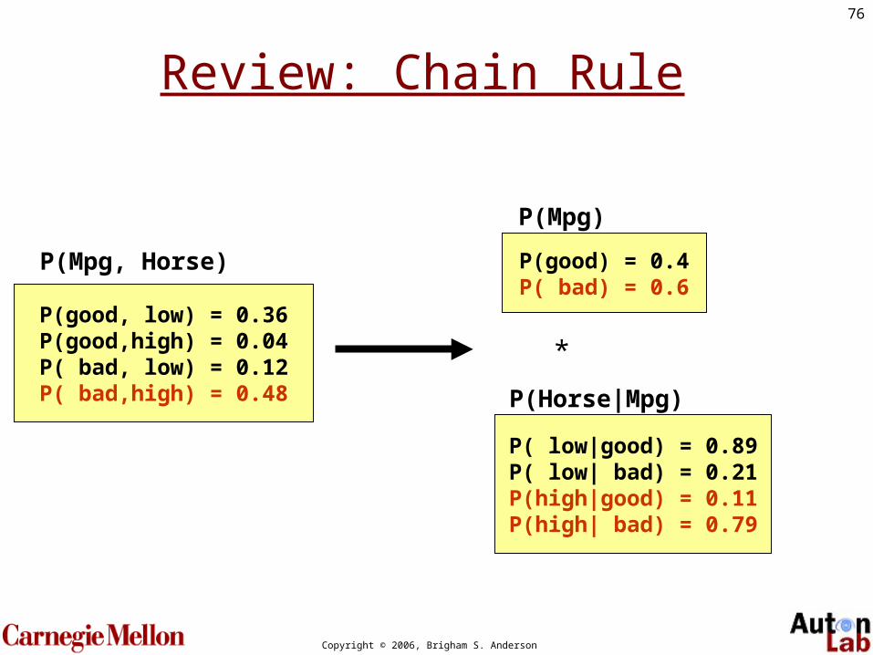
Review: Chain Rule
0.480.12bad
0.040.36good
highlow
P(Mpg, Horse)
P(good, low) = 0.36P(good,high) = 0.04P( bad, low) = 0.12P( bad,high) = 0.48
P(Mpg, Horse) P(good) = 0.4P( bad) = 0.6
P( low|good) = 0.89P( low| bad) = 0.21P(high|good) = 0.11P(high| bad) = 0.79
P(Mpg)
P(Horse|Mpg)
*

77
Copyright © 2006, Brigham S. Anderson
Review: Chain Rule
0.480.12bad
0.040.36good
highlow
P(Mpg, Horse)
P(good, low) = 0.36P(good,high) = 0.04P( bad, low) = 0.12P( bad,high) = 0.48
P(Mpg, Horse) P(good) = 0.4P( bad) = 0.6
P( low|good) = 0.89P( low| bad) = 0.21P(high|good) = 0.11P(high| bad) = 0.79
P(Mpg)
P(Horse|Mpg)
*
= P(good) * P(low|good) = 0.4 * 0.89
= P(good) * P(high|good) = 0.4 * 0.11
= P(bad) * P(low|bad) = 0.6 * 0.21
= P(bad) * P(high|bad) = 0.6 * 0.79

78
Copyright © 2006, Brigham S. Anderson
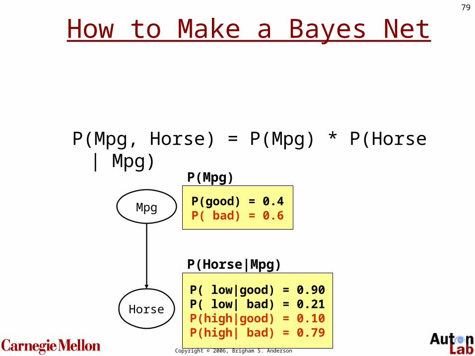
How to Make a Bayes Net
P(Mpg, Horse) = P(Mpg) * P(Horse | Mpg)
Mpg
Horse
79
Copyright © 2006, Brigham S. Anderson
How to Make a Bayes Net
P(Mpg, Horse) = P(Mpg) * P(Horse | Mpg)
Mpg
Horse
P(good) = 0.4P( bad) = 0.6
P(Mpg)
P( low|good) = 0.90P( low| bad) = 0.21P(high|good) = 0.10P(high| bad) = 0.79
P(Horse|Mpg)

80
Copyright © 2006, Brigham S. Anderson
How to Make a Bayes Net
Mpg
Horse
P(good) = 0.4P( bad) = 0.6
P(Mpg)
P( low|good) = 0.90P( low| bad) = 0.21P(high|good) = 0.10P(high| bad) = 0.79
P(Horse|Mpg)
• Each node is a probability function
• Each arc denotes conditional dependence

81
Copyright © 2006, Brigham S. Anderson
How to Make a Bayes Net
So, what have we accomplished thus far?
Nothing; we’ve just “Bayes Net-ified” the
P(Mpg, Horse) JPT using the Chain rule.
…the real excitement starts when we wield conditional independence
Mpg
Horse
P(Mpg)
P(Horse|Mpg)

82
Copyright © 2006, Brigham S. Anderson
How to Make a Bayes Net
Before we continue, we need a worthier opponent than puny P(Mpg, Horse)…
We’ll use P(Mpg, Horse, Accel):
P(good, low,slow) = 0.37P(good, low,fast) = 0.01P(good,high,slow) = 0.02P(good,high,fast) = 0.00P( bad, low,slow) = 0.10P( bad, low,fast) = 0.12P( bad,high,slow) = 0.16P( bad,high,fast) = 0.22
P(Mpg,Horse,Accel)
* Note: I made these up…

83
Copyright © 2006, Brigham S. Anderson
How to Make a Bayes Net
Step 1: Rewrite joint using the Chain rule.
P(Mpg, Horse, Accel) = P(Mpg) P(Horse | Mpg) P(Accel | Mpg, Horse)
Note:Obviously, we could have written this 3!=6 different ways…
P(M, H, A) = P(M) * P(H|M) * P(A|M,H) = P(M) * P(A|M) * P(H|M,A) = P(H) * P(M|H) * P(A|H,M) = P(H) * P(A|H) * P(M|H,A) = … = …

84
Copyright © 2006, Brigham S. Anderson
How to Make a Bayes Net
Mpg
Horse
Accel
Step 1: Rewrite joint using the Chain rule.
P(Mpg, Horse, Accel) = P(Mpg) P(Horse | Mpg) P(Accel | Mpg, Horse)

85
Copyright © 2006, Brigham S. Anderson
How to Make a Bayes Net
Mpg
Horse
Accel
P(Mpg)
P(Horse|Mpg)
P(Accel|Mpg,Horse)

86
Copyright © 2006, Brigham S. Anderson
How to Make a Bayes Net
Mpg
Horse
Accel
P(good) = 0.4P( bad) = 0.6
P(Mpg)
P( low|good) = 0.90P( low| bad) = 0.21P(high|good) = 0.10P(high| bad) = 0.79
P(Horse|Mpg)
P(slow|good, low) = 0.97P(slow|good,high) = 0.15P(slow| bad, low) = 0.90P(slow| bad,high) = 0.05P(fast|good, low) = 0.03P(fast|good,high) = 0.85P(fast| bad, low) = 0.10P(fast| bad,high) = 0.95
P(Accel|Mpg,Horse)
* Note: I made these up too…

87
Copyright © 2006, Brigham S. Anderson
How to Make a Bayes Net
Mpg
Horse
Accel
P(good) = 0.4P( bad) = 0.6
P(Mpg)
P( low|good) = 0.89P( low| bad) = 0.21P(high|good) = 0.11P(high| bad) = 0.79
P(Horse|Mpg)
P(slow|good, low) = 0.97P(slow|good,high) = 0.15P(slow| bad, low) = 0.90P(slow| bad,high) = 0.05P(fast|good, low) = 0.03P(fast|good,high) = 0.85P(fast| bad, low) = 0.10P(fast| bad,high) = 0.95
P(Accel|Mpg,Horse)
A Miracle Occurs!
You are told by God (or another domain expert)that Accel is independent of Mpg given Horse!
i.e., P(Accel | Mpg, Horse) = P(Accel | Horse)

88
Copyright © 2006, Brigham S. Anderson
How to Make a Bayes Net
Mpg
Horse
Accel
P(good) = 0.4P( bad) = 0.6
P(Mpg)
P( low|good) = 0.89P( low| bad) = 0.21P(high|good) = 0.11P(high| bad) = 0.79
P(Horse|Mpg)
P(slow| low) = 0.22P(slow|high) = 0.64P(fast| low) = 0.78P(fast|high) = 0.36
P(Accel|Horse)

89
Copyright © 2006, Brigham S. Anderson
How to Make a Bayes Net
Mpg
Horse
Accel
P(good) = 0.4P( bad) = 0.6
P(Mpg)
P( low|good) = 0.89P( low| bad) = 0.21P(high|good) = 0.11P(high| bad) = 0.79
P(Horse|Mpg)
P(slow| low) = 0.22P(slow|high) = 0.64P(fast| low) = 0.78P(fast|high) = 0.36
P(Accel|Horse)
Thank you, domain expert!
Now I only need to learn 5 parameters
instead of 7 from my data!
My parameter estimateswill be more accurate as
a result!

90
Copyright © 2006, Brigham S. Anderson
Independence“The Acceleration does not depend on the Mpg once I know the Horsepower.”
This can be specified very simply:
P(Accel Mpg, Horse) = P(Accel | Horse)
This is a powerful statement!
It required extra domain knowledge. A different kind of knowledge than numerical probabilities. It needed an understanding of causation.

91
Copyright © 2006, Brigham S. Anderson
Bayes Nets Formalized
A Bayes net (also called a belief network) is an augmented directed acyclic graph, represented by the pair V , E where:
• V is a set of vertices.• E is a set of directed edges joining vertices. No loops
of any length are allowed.
Each vertex in V contains the following information:• A Conditional Probability Table (CPT) indicating how
this variable’s probabilities depend on all possible combinations of parental values.

92
Copyright © 2006, Brigham S. Anderson
Bayes Nets Summary
• Bayes nets are a factorization of the full JPT which uses the chain rule and conditional independence.
• They can do everything a JPT can do (like quick, cheap lookups of probabilities)

93
Copyright © 2006, Brigham S. Anderson
The good news
We can do inference.
We can compute any conditional probability:
P( Some variable Some other variable values )
2
2 1
matching entriesjoint
and matching entriesjoint
2
2121 )entryjoint (
)entryjoint (
)(
)()|(
E
EE
P
P
EP
EEPEEP

94
Copyright © 2006, Brigham S. Anderson
The good news
We can do inference.
We can compute any conditional probability:
P( Some variable Some other variable values )
2
2 1
matching entriesjoint
and matching entriesjoint
2
2121 )entryjoint (
)entryjoint (
)(
)()|(
E
EE
P
P
EP
EEPEEP
Suppose you have m binary-valued variables in your Bayes Net and expression E2 mentions k variables.
How much work is the above computation?
95
Copyright © 2006, Brigham S. Anderson
The sad, bad news
Doing inference “JPT-style” by enumerating all matching entries in the joint are expensive:
Exponential in the number of variables.
But perhaps there are faster ways of querying Bayes nets?• In fact, if I ever ask you to manually do a Bayes Net inference, you’ll find
there are often many tricks to save you time.• So we’ve just got to program our computer to do those tricks too, right?
Sadder and worse news:General querying of Bayes nets is NP-complete.

96
Copyright © 2006, Brigham S. Anderson
Case Study I
Pathfinder system. (Heckerman 1991, Probabilistic Similarity Networks, MIT Press, Cambridge MA).
• Diagnostic system for lymph-node diseases.
• 60 diseases and 100 symptoms and test-results.
• 14,000 probabilities
• Expert consulted to make net.
• 8 hours to determine variables.
• 35 hours for net topology.
• 40 hours for probability table values.
• Apparently, the experts found it quite easy to invent the causal links and probabilities.
• Pathfinder is now outperforming the world experts in diagnosis. Being extended to several dozen other medical domains.

97
Copyright © 2006, Brigham S. Anderson
Bayes Net Info
GUI Packages:• Genie -- Free • Netica -- $$• Hugin -- $$
Non-GUI Packages:• All of the above have APIs• BNT for MATLAB• AUTON code (learning extremely large networks of tens
of thousands of nodes)

98
Copyright © 2006, Brigham S. Anderson
Bayes Nets andMachine Learning

99
Copyright © 2006, Brigham S. Anderson
Machine Learning Tasks
ClassifierData point x
AnomalyDetector
Data point x P(x)
P(C | x)
Inference
Engine
Evidence e1P(e2 | e1) Missing Variables e2

100
Copyright © 2006, Brigham S. Anderson
What is an Anomaly?
• An irregularity that cannot be explained by simple domain models and knowledge
• Anomaly detection only needs to learn from examples of “normal” system behavior.
• Classification, on the other hand, would need examples labeled “normal” and “not-normal”

101
Copyright © 2006, Brigham S. Anderson
Anomaly Detection in Practice
• Monitoring computer networks for attacks.
• Monitoring population-wide health data for outbreaks or attacks.
• Looking for suspicious activity in bank transactions
• Detecting unusual eBay selling/buying behavior.

102
Copyright © 2006, Brigham S. Anderson
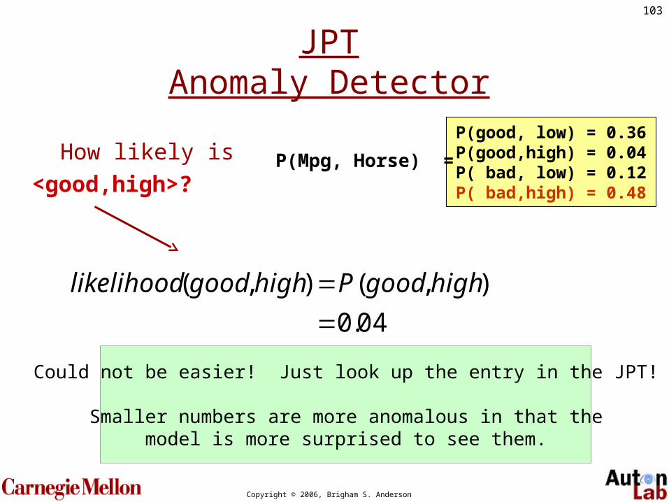
JPTAnomaly Detector
• Suppose we have the following model:
P(good, low) = 0.36P(good,high) = 0.04P( bad, low) = 0.12P( bad,high) = 0.48
P(Mpg, Horse) =
• We’re trying to detect anomalous cars.
• If the next example we see is <good,high>, how anomalous is it?
103
Copyright © 2006, Brigham S. Anderson
JPTAnomaly Detector
04.0
),(),(
highgoodPhighgoodlikelihood
P(good, low) = 0.36P(good,high) = 0.04P( bad, low) = 0.12P( bad,high) = 0.48
P(Mpg, Horse) = How likely is
<good,high>?
Could not be easier! Just look up the entry in the JPT!
Smaller numbers are more anomalous in that themodel is more surprised to see them.

104
Copyright © 2006, Brigham S. Anderson
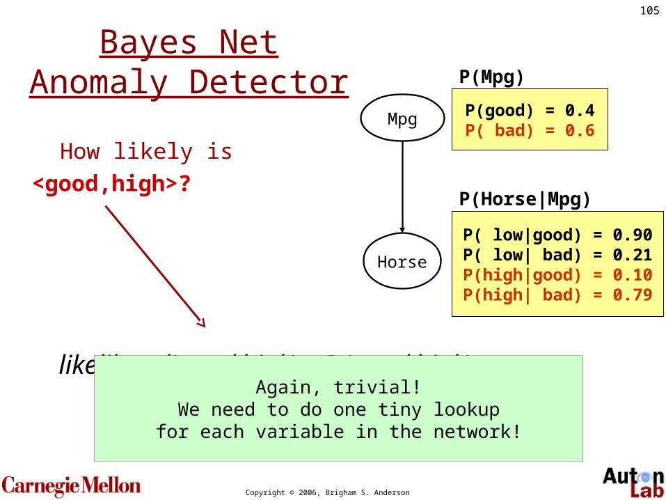
Bayes NetAnomaly Detector
04.0
)|()(
),(),(
goodhighPgoodP
highgoodPhighgoodlikelihood
How likely is
<good,high>?
Mpg
Horse
P(good) = 0.4P( bad) = 0.6
P(Mpg)
P( low|good) = 0.90P( low| bad) = 0.21P(high|good) = 0.10P(high| bad) = 0.79
P(Horse|Mpg)
105
Copyright © 2006, Brigham S. Anderson
Bayes NetAnomaly Detector
04.0
)|()(
),(),(
goodhighPgoodP
highgoodPhighgoodlikelihood
How likely is
<good,high>?
Mpg
Horse
P(good) = 0.4P( bad) = 0.6
P(Mpg)
P( low|good) = 0.90P( low| bad) = 0.21P(high|good) = 0.10P(high| bad) = 0.79
P(Horse|Mpg)
Again, trivial!We need to do one tiny lookup
for each variable in the network!

106
Copyright © 2006, Brigham S. Anderson
Machine Learning Tasks
ClassifierData point x
AnomalyDetector
Data point x P(x)
P(C | x)
Inference
Engine
Evidence e1P(E2 | e1) Missing Variables E2

107
Copyright © 2006, Brigham S. Anderson
Bayes Classifiers
• A formidable and sworn enemy of decision trees
DT BC
108
Copyright © 2006, Brigham S. Anderson
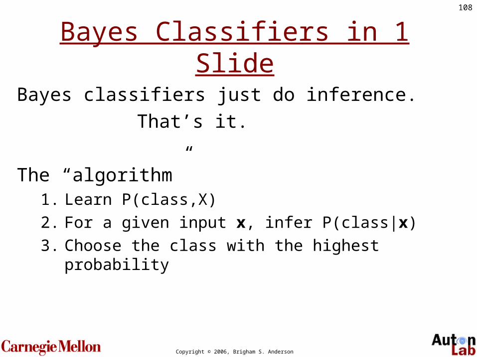
Bayes Classifiers in 1 Slide
Bayes classifiers just do inference.
That’s it.
The “algorithm”1. Learn P(class,X)
2. For a given input x, infer P(class|x)
3. Choose the class with the highest probability

109
Copyright © 2006, Brigham S. Anderson
JPTBayes Classifier
• Suppose we have the following model:
P(good, low) = 0.36P(good,high) = 0.04P( bad, low) = 0.12P( bad,high) = 0.48
P(Mpg, Horse) =
• We’re trying to classify cars as Mpg = “good” or “bad”
• If the next example we see is Horse = “low”, how do we classify it?

110
Copyright © 2006, Brigham S. Anderson
JPTBayes Classifier
)(
),()|(
lowP
lowgoodPlowgoodP
P(good, low) = 0.36P(good,high) = 0.04P( bad, low) = 0.12P( bad,high) = 0.48
P(Mpg, Horse) =
),(),(
),(
lowbadPlowgoodP
lowgoodP
739.012.036.0
36.0
How do we classify
<Horse=low>?
The P(good | low) = 0.75,so we classify the example
as “good”

111
Copyright © 2006, Brigham S. Anderson
Bayes Net Classifier
Mpg
Horse
Accel
P(good) = 0.4P( bad) = 0.6
P(Mpg)
P( low|good) = 0.89P( low| bad) = 0.21P(high|good) = 0.11P(high| bad) = 0.79
P(Horse|Mpg)
P(slow| low) = 0.95P(slow|high) = 0.11P(fast| low) = 0.05P(fast|high) = 0.89
P(Accel|Horse)
• We’re trying to classify cars as Mpg = “good” or “bad”
• If the next example we see is <Horse=low,Accel=fast> how do we classify it?
112
Copyright © 2006, Brigham S. Anderson
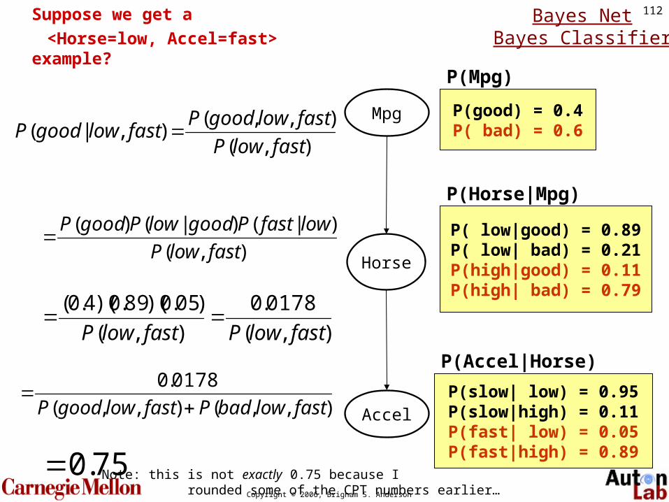
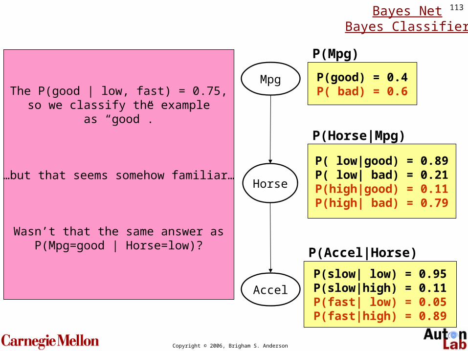
Suppose we get a
<Horse=low, Accel=fast> example?
),(
),,(),|(
fastlowP
fastlowgoodPfastlowgoodP
Mpg
Horse
Accel
P(good) = 0.4P( bad) = 0.6
P(Mpg)
P( low|good) = 0.89P( low| bad) = 0.21P(high|good) = 0.11P(high| bad) = 0.79
P(Horse|Mpg)
P(slow| low) = 0.95P(slow|high) = 0.11P(fast| low) = 0.05P(fast|high) = 0.89
P(Accel|Horse)
),(
)|()|()(
fastlowP
lowfastPgoodlowPgoodP
),(
0178.0
),(
)05.0)(89.0)(4.0(
fastlowPfastlowP
),,(),,(
0178.0
fastlowbadPfastlowgoodP
75.0 Note: this is not exactly 0.75 because I rounded some of the CPT numbers earlier…
Bayes NetBayes Classifier
113
Copyright © 2006, Brigham S. Anderson
Mpg
Horse
Accel
P(good) = 0.4P( bad) = 0.6
P(Mpg)
P( low|good) = 0.89P( low| bad) = 0.21P(high|good) = 0.11P(high| bad) = 0.79
P(Horse|Mpg)
P(slow| low) = 0.95P(slow|high) = 0.11P(fast| low) = 0.05P(fast|high) = 0.89
P(Accel|Horse)
The P(good | low, fast) = 0.75,so we classify the example
as “good”.
…but that seems somehow familiar…
Wasn’t that the same answer asP(Mpg=good | Horse=low)?
Bayes NetBayes Classifier

114
Copyright © 2006, Brigham S. Anderson
Bayes Classifiers
• OK, so classification can be posed as inference
• In fact, virtually all machine learning tasks are a form of inference
• Anomaly detection: P(x)• Classification: P(Class | x)• Regression: P(Y | x)• Model Learning: P(Model | dataset)• Feature Selection: P(Model | dataset)

115
Copyright © 2006, Brigham S. Anderson
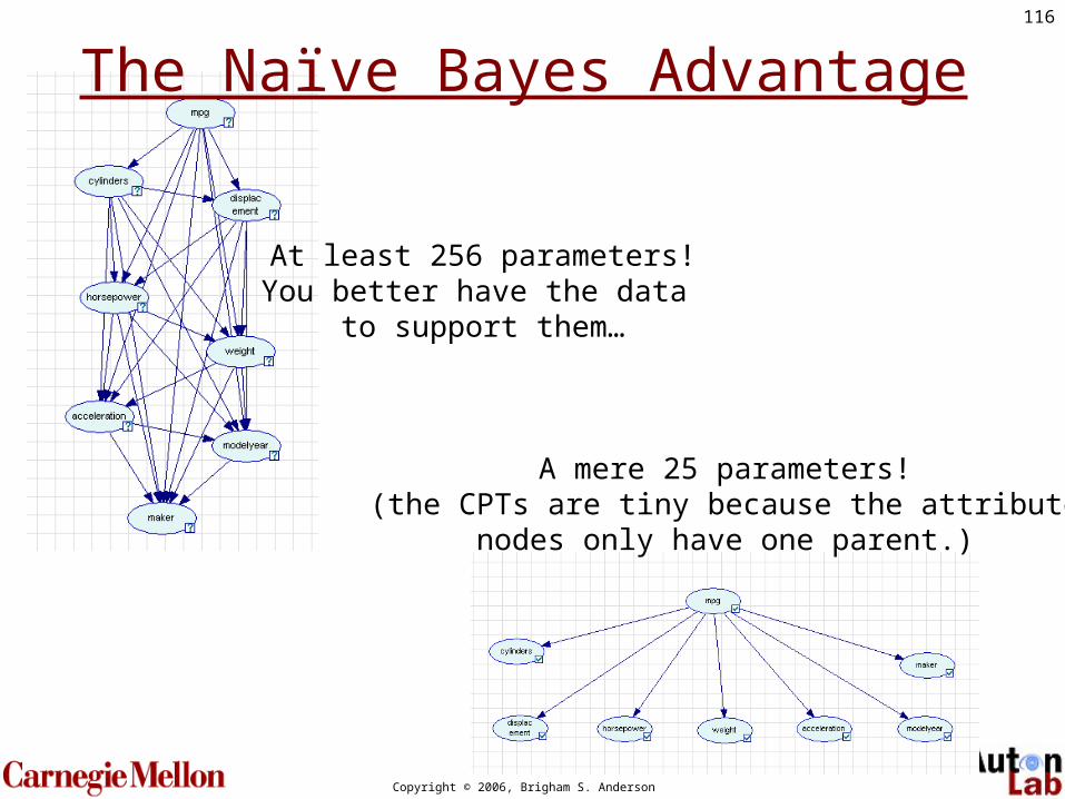
The Naïve Bayes Classifier
ASSUMPTION: all the attributes are conditionally independent
given the class variable
116
Copyright © 2006, Brigham S. Anderson
At least 256 parameters!You better have the data
to support them…
A mere 25 parameters!(the CPTs are tiny because the attribute
nodes only have one parent.)
The Naïve Bayes Advantage

117
Copyright © 2006, Brigham S. Anderson
What is the Probability Functionof the Naïve Bayes?
P(Mpg,Cylinders,Weight,Maker,…) =
P(Mpg) P(Cylinders|Mpg) P(Weight|Mpg) P(Maker|Mpg) …

118
Copyright © 2006, Brigham S. Anderson
What is the Probability Functionof the Naïve Bayes?
i
i classxPclassPclassP )|()(),( x
This is another great feature of Bayes Nets; you can graphically
see your model assumptions

119
Copyright © 2006, Brigham S. Anderson
Bayes Classifier Results: “MPG”:
392 records
The Classifier
learned by “Naive BC”

120
Copyright © 2006, Brigham S. Anderson
Bayes Classifier Results: “MPG”:
40 records

121
Copyright © 2006, Brigham S. Anderson
More Facts About Bayes Classifiers
• Many other density estimators can be slotted in
• Density estimation can be performed with real-valued inputs
• Bayes Classifiers can be built with real-valued inputs
• Rather Technical Complaint: Bayes Classifiers don’t try to be maximally discriminative---they merely try to honestly model what’s going on
• Zero probabilities are painful for Joint and Naïve. A hack (justifiable with the magic words “Dirichlet Prior”) can help.
• Naïve Bayes is wonderfully cheap. And survives 10,000 attributes cheerfully!

122
Copyright © 2006, Brigham S. Anderson
Summary
• Axioms of Probability
• Bayes nets are created by• chain rule• conditional independence
• Bayes Nets can do• Inference• Anomaly Detection• Classification

123
Copyright © 2006, Brigham S. Anderson

124
Copyright © 2006, Brigham S. Anderson
The Axioms Of Probability