copyright by celia hubert lopez 2011

Copyright

by

Celia Hubert Lopez

2011

The Thesis Committee for Celia Hubert Lopez

Certifies that this is the approved version of the following thesis:

Municipality Characteristics and Math Achievement: A Multilevel

Analysis of Mexican Secondary Schools

APPROVED BY

SUPERVISING COMMITTEE:

Joseph E. Potter

Leticia J. Marteleto

Supervisor:



by

Celia Hubert Lopez, BA.

Thesis

Presented to the Faculty of the Graduate School of

The University of Texas at Austin

in Partial Fulfillment

of the Requirements

for the Degree of

Master of Arts

The University of Texas at Austin

May 2011

Dedication

A mis padres con amor. Gracias por su apoyo incondicional en cada momento de mi vida.

v

Acknowledgements

I want to express my gratitude to Joseph Potter and Leticia Marteleto, my advisor

and reader, for the critical comments and suggestions provided.

I am extremely grateful to Amanda Stevenson, who helped me reading and

editing this Thesis.

May 4, 2011

vi

Abstract



Celia Hubert Lopez, M.A.

The University of Texas at Austin, 2011

Supervisor: Joseph E. Potter

This study examines the impact of the municipality level characteristics on the

average Math achievement of students in third year of lower secondary schools in

Mexico. Using data from different Mexican and international sources and multi-level

regression models the present work shows that municipality characteristics provide

additional explanation of the unexplained variability in educational achievement

controlling for school-level factors and even without accounting for student

characteristics. Although school factors are highly correlated with municipality’s

characteristics, the present study finds that unobservable characteristics of the

municipality are playing an important role in Mexican students’ achievement which goes

beyond the possible impact that school factors have on achievement.

vii

Table of Contents

List of Tables ......................................................................................................... ix

INTRODUCTION 1

LITERATURE REVIEW 2

Conceptual framework ....................................................................................2

Context ............................................................................................................4

Population distribution ...........................................................................4

Wealth distribution.................................................................................4

Education ...............................................................................................5

Educational outcomes ...................................................................5

Mexican Educational System ........................................................6

ENLACE Test ...............................................................................9

Municipalities ......................................................................................11

Past research..................................................................................................13

RESEARCH QUESTION AND HYPOTHESES 15

DATA AND METHOD 16

Data .....................................................................................................16

Variables ..............................................................................................16

School level .................................................................................16

Municipality level .......................................................................18

Method .................................................................................................19

RESULTS 22

Descriptive analysis ......................................................................................22

Unconditional model .....................................................................................25

Conditional models .......................................................................................26

School characteristics..................................................................26

Municipalities’ characteristics ....................................................29

viii

CONCLUSION 33

LIMITATIONS 34

Appendix A ............................................................................................................35

References ..............................................................................................................37

ix

List of Tables

Table 1. Average number of years of schooling by poverty condition. ...................6

Table 2. Mexican Educational System .....................................................................7

Table 3. Lower secondary education, 2005 .............................................................8

Table 4. ENLACE average scores for 3rd grade students in secondary level by type of

school, 2006 ......................................................................................10

Table 5. Descriptive statistics for school level variables .......................................22

Table 6. Descriptive statistics for municipality level variables .............................24

Table 7. Results from the Unconditional Model ....................................................25

Table 8. Conditional models with school-level covariates ....................................28

Table 9. Correlation matrix for municipality variables .........................................29

Table 10. Conditional models with school and municipality covariates ...............30

Table 11. Final model ............................................................................................32

Table A. Descriptive statistics for school level variables by type of school .........35

1

INTRODUCTION

Diversity pervades every aspect of Mexico; communities in the country are

culturally, socioeconomically, and environmentally diverse. Education represents one of

the characteristics with significant between-community disparities. The Mexican

education system has been characterized by its deep and geographically reproduced

inequality (Gutierrez, Giorguli, and Sanchez 2010). While there have been studies of the

influence of family and schools on educational outcomes, examinations of the influence

of community factors on educational outcomes are rare for developing countries

(Buchmann and Hannum 2001). In Mexico, municipality is the smallest unit of

government with the authority to implement public policies and as such municipalities

influence the schools under their jurisdiction. Knowing the extent to which municipalities

influence school effectiveness could guide the targeting of policies to improve Mexican

education. The present study analyzes the impact of municipality characteristics on the

achievement of secondary school students in Mexico.

2

LITERATURE REVIEW

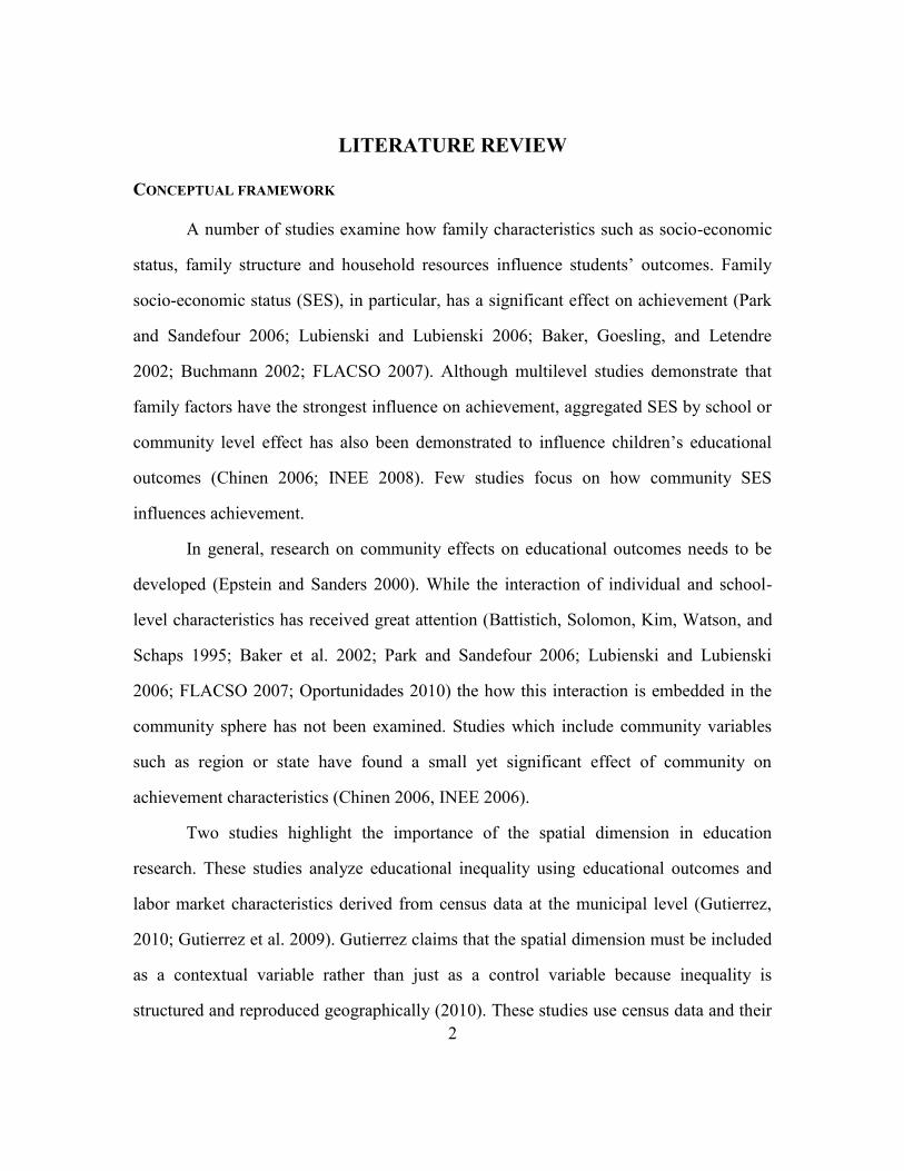
CONCEPTUAL FRAMEWORK

A number of studies examine how family characteristics such as socio-economic

status, family structure and household resources influence students’ outcomes. Family

socio-economic status (SES), in particular, has a significant effect on achievement (Park

and Sandefour 2006; Lubienski and Lubienski 2006; Baker, Goesling, and Letendre

2002; Buchmann 2002; FLACSO 2007). Although multilevel studies demonstrate that

family factors have the strongest influence on achievement, aggregated SES by school or

community level effect has also been demonstrated to influence children’s educational

outcomes (Chinen 2006; INEE 2008). Few studies focus on how community SES

influences achievement.

In general, research on community effects on educational outcomes needs to be

developed (Epstein and Sanders 2000). While the interaction of individual and school-

level characteristics has received great attention (Battistich, Solomon, Kim, Watson, and

Schaps 1995; Baker et al. 2002; Park and Sandefour 2006; Lubienski and Lubienski

2006; FLACSO 2007; Oportunidades 2010) the how this interaction is embedded in the

community sphere has not been examined. Studies which include community variables

such as region or state have found a small yet significant effect of community on

achievement characteristics (Chinen 2006, INEE 2006).

Two studies highlight the importance of the spatial dimension in education

research. These studies analyze educational inequality using educational outcomes and

labor market characteristics derived from census data at the municipal level (Gutierrez,

2010; Gutierrez et al. 2009). Gutierrez claims that the spatial dimension must be included

as a contextual variable rather than just as a control variable because inequality is

structured and reproduced geographically (2010). These studies use census data and their

3

outcome measure is therefore limited to educational attainment which measures only

quantity of education not quality.

Santibañez (2008) explains that measuring educational inequality as number of

years of education could yield to misleading results. For instance, she says, countries with

high levels of income inequality usually experience high levels of educational inequality.

However, despite Latin American countries’ high income inequality, educational

inequality in Latin America is not as high as could be expected (De Ferranti cited in

Santibañez 2008). Students with the same number of years of education might have very

different levels of knowledge. Santibañez (2008) states that ―the knowledge acquired by a

child with 7 or 8 years of schooling in Mexico is not the same as the knowledge acquired

by a child with the same number of years of schooling in South Korea or Finland, which

is why quality seems to be a more important factor than the number of years of

education‖.

Regarding school quality, several studies show that school-level measures of

teachers’ characteristics are related to students’ achievement (McKinsey & Co. 2008;

LLECE 2001; UNESCO 1999; Villegas-Reimers and Reimers 1996). Teachers’ salary

could be used as a measure of quality under the assumption that better teachers tend to

earn higher wages. However, in countries like Mexico where teachers’ salaries do not

depend on their performance other measures must be used.

4

CONTEXT

In 2005, Mexico had a population of 103.3 million people distributed into 31

states and one Federal District (INEGI 2005a). In this year, Mexican Gross Domestic

Product (GDP) per capita was 12,461 USD (OECD 2010). The average number of years

of schooling in 2005 was 8.1, the literacy rate was 91.6%, more than 75% of people 15

years old or older had completed primary school, almost 54% of this population had

completed secondary school, and 32% had completed high school. Enrollment in school

differs in each age group. Almost all children between 6 and 12 years old attend school

(96.1%), 82.5% of the teenagers between 13 to 15 years old, 47.8% of the teenagers

between 16 to 19 years old, and 20.8% of adults between 20 and 24 years old are enrolled

in school (INEGI 2005a).

As other countries in Latin America, Mexico has experience a historical

inequality in the distribution of its population, wealth and education. This uneven

distribution becomes evident when data are analyzed using different layers such as

poverty level or urban or rural areas.

Population distribution

In 2005, Mexican population was distributed among 187,938 localities; 23.5% of

this population lived in 184,748 localities with less than 2,500 inhabitants (INEGI

2005a). Around 12.9% (13.4 million people) of the population was indigenous and

around 12% of this indigenous population does not speak Spanish. 73.5% of the

indigenous population is concentrated in 11 of the 32 states (CONAPO 2005).

Wealth distribution

The generation of wealth is also unequal as 85% of GDP is produced in urban

areas and only 15% in rural areas. At the individual level inequality is more evident,

5

according to the National Council for the Evaluation of Social Development Policy

(CONEVAL, its acronym in Spanish), in 2005, on average the income of the richest 5

percent of the population was 52.7 times higher than that of the poorest 5 percent

(CONEVAL 2007). Furthermore, CONEVAL reports that in this year 17.4% of the total

population was below the food poverty line, 24.7% suffered from poverty of capacities,

while 47.2% were below the patrimony poverty line (2007).1 The percentage of the

population in poverty conditions in rural settings is much higher than the percentages

observed in urban areas. In rural areas 28% percent of the population was below the food

poverty line, 36.2% were below the capacities poverty line and 57.4% below the

patrimony poverty line, whereas only 11% of the people in urban areas were below the

food poverty line, 17.8% and 41.1% were below the capacities and patrimony lines

respectively.

Education

Educational outcomes

Although Mexico has improved its educational outcomes -such as literacy rates,

average number of years of schooling, and attainment rates- over time those

improvements have not been equally distributed among the population. In 1921, 66% of

the population was illiterate whereas in 2005 8.4% was. However, the percentage of

illiterate people in rural areas in 2005 was 18.9% and only 5.3% in urban areas.

Comparing population by poverty condition, the difference is even large 20.9% of the

people below the capacities poverty line were illiterate while only 3.4% among the non-

1 ―Food poverty takes into account the population without enough income to buy a basic food basket: the

poverty of capacities considers the population without enough income to simultaneously satisfy their needs

for food, health and education: the poverty of patrimony considers the population without enough income

to satisfy food, health, education, shelter, public transport, clothing and footwear needs.‖ (CTPM 2002)

Those who are below the food poverty line are also considered capacities and patrimony poor.

6

poor were2. Additionally, 67% of the illiterate population between 15 and 34 years old is

concentrated in 8 states: Chiapas (15.7%), Veracruz (11.9%), Puebla (8.2%), Guerrero

(7.8%), México (6.7%), Oaxaca (6.6%), Michoacán (5.5%), and Guanajuato (4.4%).

The national average number of years of schooling in 2005 was 8.1 compared

with the national average of 2.6 years in 1960 the improvement is clear, but this change

has not been equal across the country. For instance, in the country’s capital (Distrito

Federal), the average was 10.2, while Chiapas’ averaged only 6.1. As with the illiteracy

rate, inequality becomes more noticeable when comparing poor3 and non poor

population. While non poor average 9.6 years of education, poor people only have 5.2

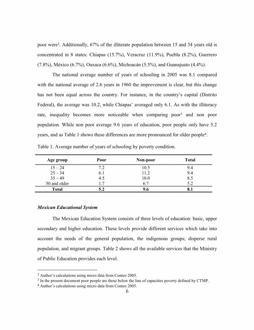
years, and as Table 1 shows these differences are more pronounced for older people4.

Table 1. Average number of years of schooling by poverty condition.

Age group Poor Non-poor Total

15 – 24 7.2 10.5 9.4

25 – 34 6.1 11.2 9.4

35 – 49 4.5 10.0 8.5

50 and older 1.7 6.7 5.2

Total 5.2 9.6 8.1

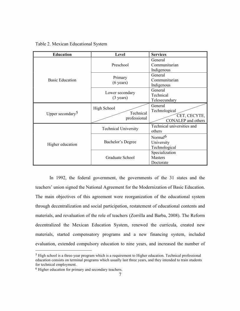
Mexican Educational System

The Mexican Education System consists of three levels of education: basic, upper

secondary and higher education. These levels provide different services which take into

account the needs of the general population, the indigenous groups; disperse rural

population, and migrant groups. Table 2 shows all the available services that the Ministry

of Public Education provides each level.

2 Author’s calculations using micro data from Conteo 2005. 3 In the present document poor people are those below the line of capacities poverty defined by CTMP. 4 Author’s calculations using micro data from Conteo 2005.

7

Table 2. Mexican Educational System

Education Level Services

Basic Education

Preschool

General

Communitarian

Indigenous

Primary

(6 years)

General

Communitarian

Indigenous

Lower secondary

(3 years)

General

Technical

Telesecundary

Upper secondary5

High School

Technical

professional

General

Technological

CET, CECYTE,

CONALEP and others

Higher education

Technical University Technical universities and

others

Bachelor’s Degree Normal6

University

Technological

Graduate School

Specialization

Masters

Doctorate

In 1992, the federal government, the governments of the 31 states and the

teachers’ union signed the National Agreement for the Modernization of Basic Education.

The main objectives of this agreement were reorganization of the educational system

through decentralization and social participation, restatement of educational contents and

materials, and revaluation of the role of teachers (Zorrilla and Barba, 2008). The Reform

decentralized the Mexican Education System, renewed the curricula, created new

materials, started compensatory programs and a new financing system, included

evaluation, extended compulsory education to nine years, and increased the number of

5 High school is a three-year program which is a requirement to Higher education. Technical professional

education consists on terminal programs which usually last three years, and they intended to train students

for technical employment. 6 Higher education for primary and secondary teachers.

8

school days (Zorrilla, 2002). These changes were legitimized with the amendment to

Article 3 of the Constitution which includes the compulsory lower secondary education

and the enactment of the Education Act adopted in 1993.

Lower secondary7 level of education is the third and last level of compulsory

education. It is completed in three years. It is a requirement to enter upper secondary.

There are three different types of secondary schools: General, technical and

Telesecondary. General secondary is the most common type which provides general

studies to fulfill the required knowledge to enter the following level. Technical secondary

provides a technical degree which allows students to enter the job market after finishing

it. The telesecondary (or Telesecundaria) was launched in 1968 as a means of extending

lower secondary school learning with television support to remote and small communities

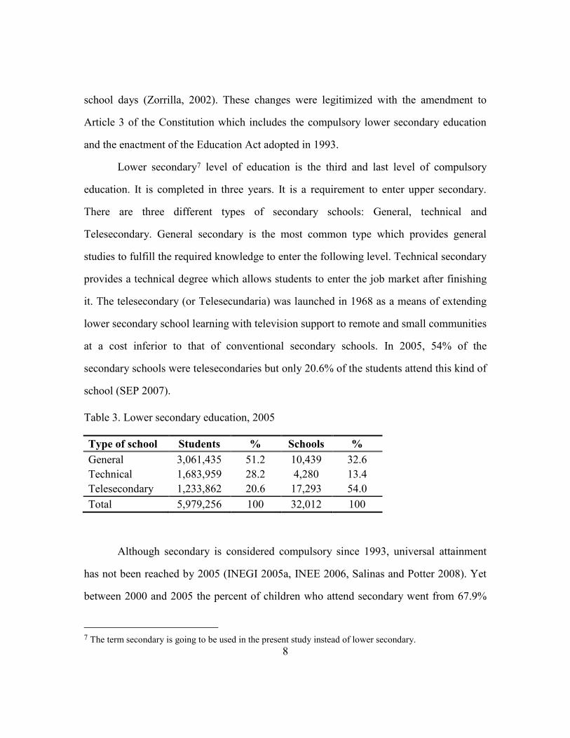
at a cost inferior to that of conventional secondary schools. In 2005, 54% of the

secondary schools were telesecondaries but only 20.6% of the students attend this kind of

school (SEP 2007).

Table 3. Lower secondary education, 2005

Type of school Students % Schools %

General 3,061,435 51.2 10,439 32.6

Technical 1,683,959 28.2 4,280 13.4

Telesecondary 1,233,862 20.6 17,293 54.0

Total 5,979,256 100 32,012 100

Although secondary is considered compulsory since 1993, universal attainment

has not been reached by 2005 (INEGI 2005a, INEE 2006, Salinas and Potter 2008). Yet

between 2000 and 2005 the percent of children who attend secondary went from 67.9%

7 The term secondary is going to be used in the present study instead of lower secondary.

9

to 77.6%. The telesecondary plays an important role in the increase of secondary

attainment. However, this type of secondary offers a very low quality education which

results in poor outcomes in international and national evaluations (INEE 2006, Salinas

and Potter 2008, Chinen 2006).

ENLACE Test

If as Santibañez argues, improving the quality of education yields economic

development and equality of opportunities among the population (2008), making

measuring the quality of education very important for Mexican educational authorities.

Since 2006 the Ministry of Public Education has administered the National Evaluation of

Academic Achievement in Scholar Centers (ENLACE for its acronym in Spanish)

nationwide. The ENLACE evaluates students at the primary, secondary and upper

secondary school levels. Only some grades are evaluated in primary (3rd to 6th grade)

and upper secondary levels (only 3rd grade). Since 2009 all grades of the secondary level

have been evaluated.

Scores on the ENLACE range between 200 and 800 points and reflect not only

the number of correct answers but also the level of difficulty of the questions. In 2006,

the national mean score for Mathematics and Reading in third grade of secondary was

500 with a standard deviation of 100. The ministry classified scores into four levels of

achievement based on cut off points:

1. Insufficient: The student has not achieved the required knowledge for the

subject. (Score lower than 350).

2. Basic: The student needs to improve her knowledge of the subject. (Score

equal or higher than 350 and less than 500).

10

3. Fair: The student shows an adequate knowledge for the subject. (Score

equal or higher than 500 and less than 650).

4. Excellent: The student has mastered the required knowledge for the

subject. (Score equal or higher than 650).

The aggregate results by school, type of school, and state are publicly available at

the ENLACE website8. In addition, students and their parents receive a detailed report of

students’ test results. Teachers also receive a detailed report on the performance of their

class as well as some feedback on what they can do to improve their students’ preparation

based on their students’ mistakes.

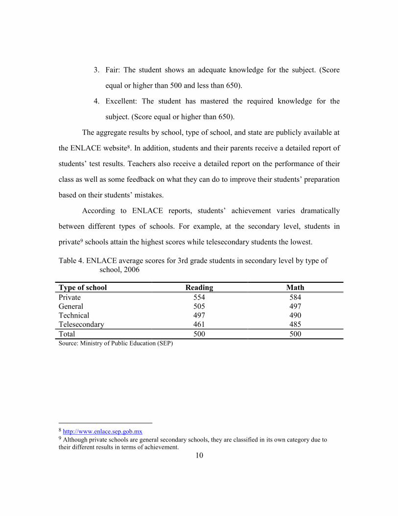
According to ENLACE reports, students’ achievement varies dramatically

between different types of schools. For example, at the secondary level, students in

private9 schools attain the highest scores while telesecondary students the lowest.

Table 4. ENLACE average scores for 3rd grade students in secondary level by type of

school, 2006

Type of school Reading Math

Private 554 584

General 505 497

Technical 497 490

Telesecondary 461 485

Total 500 500 Source: Ministry of Public Education (SEP)

8 http://www.enlace.sep.gob.mx 9 Although private schools are general secondary schools, they are classified in its own category due to

their different results in terms of achievement.

http://www.enlace.sep.gob.mx/

11

Municipalities

Municipalities are the smallest political-administrative unit governed by elected

authorities with an assigned budget. The importance of municipalities has grown as the

country has decentralized and there is evidence that the local administration of education

resources can enhance student achievement. Thus, there is reason to expect that

wealthier municipalities will have better student outcomes. The 1993 education reform

codified municipalities’ authority over education by assigning them specific

responsibilities like improvement and maintenance of school infrastructure. (Ley General

de Educación, Article 70).

There are large differences between municipalities as well as within them.

Municipalities vary with respect to number of localities, population size, budget,

resources, and demographic and socioeconomic characteristics.

In 2005, Mexico had 2,454 municipalities unequally distributed across the 31

states and the Federal District. The number of municipalities by state varies from 5 in

Baja California and Baja California Sur to 570 in Oaxaca. Most of the municipalities

include rural and urban communities but 902 municipalities have been classified as fully

rural because all localities within them have less than 2,500 inhabitants. Twenty three

municipalities are classified as fully urban.

The Mexican National Population Council (Spanish acronym CONAPO)

developed a composite index of marginality in order to differentiate states and

municipalities according to the impact of scarcity as experienced by the local population.

It measures the proportion of people 15 years old and older who are illiterate or did not

complete primary education, the percentage of people who live in private homes without

services such as piped water, drain or toilet, and electricity, the percentage of people who

12

live in houses with a dirt floor, the percentage of homes with some level of

overcrowding, the percentage of the employed population with incomes up to twice the

minimum wage, and the proportion of the population who live in localities with less than

5,000 inhabitants in order to describe lack of access to education, residence in poor

housing, perception of inadequate monetary income and related residency in small towns.

This index classifies municipalities into five levels of marginality: very high, high,

medium, low and very low. A municipality with higher marginality is generally worse

off than one with lower marginality. According to CONAPO, in 2005 1,251

municipalities, representing 16.5% of the population, had very high or high marginality

and 702 municipalities, representing 75.2% of the population, were ranked low or very

low marginality (CONAPO, 2007).

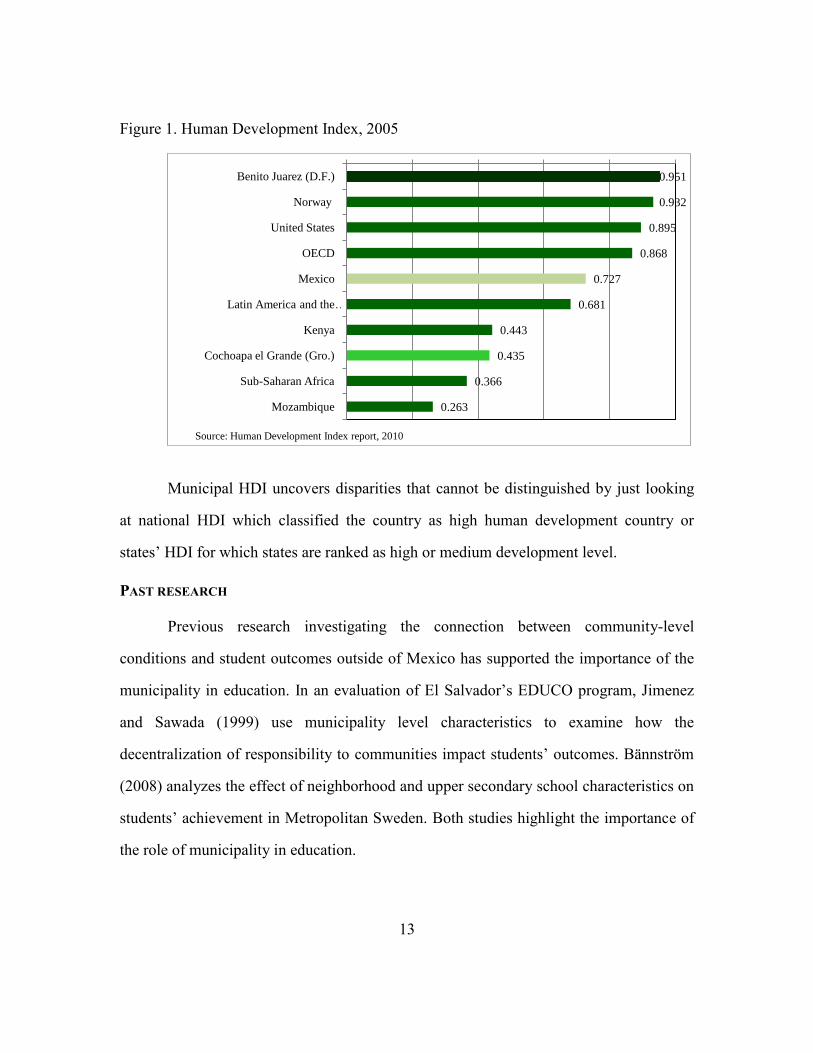
The United Nations Development Program (UNPD) calculates the Human

Development Index which is defined as ―a composite measure of achievements in three

basic dimensions of human development—a long and healthy life, access to education

and a decent standard of living. For ease of comparability, the average value of

achievements in these three dimensions is scaled to the range 0 to 1, where higher

numbers reflect higher levels of achievement, and aggregated using geometric means

(UNDP, 2008)‖. According to UNPD, Mexico as a whole had a relatively high Human

Development Index (HDI) of 0.727 in 2005. However, at the municipality level Mexico

presents a highly unequal face. For example, the municipality with the highest HDI is

Benito Juarez, which at 0.951, rates higher than the average of Organisation for

Economic Co-operation and Development (OECD) member countries. In contrast,

Cochoapa el Grande has the lowest HDI at 0.439, which is similar to countries such as

Kenya but still higher than the average of Sub-Saharan countries.

13

Figure 1. Human Development Index, 2005

Municipal HDI uncovers disparities that cannot be distinguished by just looking

at national HDI which classified the country as high human development country or

states’ HDI for which states are ranked as high or medium development level.

PAST RESEARCH

Previous research investigating the connection between community-level

conditions and student outcomes outside of Mexico has supported the importance of the

municipality in education. In an evaluation of El Salvador’s EDUCO program, Jimenez

and Sawada (1999) use municipality level characteristics to examine how the

decentralization of responsibility to communities impact students’ outcomes. Bännström

(2008) analyzes the effect of neighborhood and upper secondary school characteristics on

students’ achievement in Metropolitan Sweden. Both studies highlight the importance of

the role of municipality in education.

0.951

0.932

0.895

0.868

0.727

0.681

0.443

0.435

0.366

0.263

Benito Juarez (D.F.)

Norway

United States

OECD

Mexico

Latin America and the …

Kenya

Cochoapa el Grande (Gro.)

Sub-Saharan Africa

Mozambique

Source: Human Development Index report, 2010

14

In Mexico, there are some multilevel studies that have analyzed the impact of

community on achievement by adding it as a third level of analysis when school is the

second level. These studies include state or region level but not municipality because they

use sampling data which are not representative at the municipality level. Chinen (2006)

adds state as the third level of analysis while INEE (2006) uses region as their third level

of analysis.

Gutierrez and coauthors analyze ―the spatial dimension in the relationship

between the expected years of schooling for children living in Mexico who completed

elementary school and the dynamics of the labor markets, migration and the

characteristics of the educational services available at the municipality level (2010).‖

However, the educational variables in this study only consider grade-level attainment and

availability of education services. As mentioned above, measurements of how much

students learn at school, not just which grade they are in, is vital to efforts to understand

the factors that influence this learning process.

It is possible that municipalities explain the relationships between school and

community that are lost at state or region level. Using ENLACE data allows for an

analysis of the effect of municipality because, as a national evaluation, it is representative

at the municipality level. Multilevel analysis enables examination of the role of this

interaction in the explanation of students’ achievement. Including schools as the first

level of analysis enables an examination of whether or not community variation affects

school effectiveness.

15

RESEARCH QUESTION AND HYPOTHESES

Since there are schools nested in municipalities, the present study seeks to

investigate whether or not municipalities’ characteristics affect average school

achievement as well as how much variance in schools’ achievement is explained by

characteristics of municipalities.

Specific questions that motivate this study are:

1. How much do municipalities vary in their mean mathematics achievement?

2. Is the strength of association between school characteristics and math

achievement similar across municipalities?

3. Do schools in municipalities with higher standards of living also have better

mathematics achievement?

From these questions and the conceptual framework described above the

following hypotheses can be addressed:

1. Since municipalities are so different, it is likely that their mean mathematics

achievement varies significantly between municipalities.

2. Variability in municipal HDI highlights disparities among municipalities

which could impact education. So, it is reasonable to think that schools in

more developed municipalities could have an advantage over schools in less

developed municipalities after controlling for school characteristics.

3. Municipalities with the highest living standards are likely to have schools with

more educated and experienced teachers, which could positively influence

student achievement. Thus it can be expected that municipalities with better

living conditions will have higher student achievement.

16

DATA AND METHOD

Data

The analysis utilizes national data sets from five different sources. School

information is obtained from two national data sets. The ENLACE dataset provides the

results of the national Math and Reading examinations and the Public Education

Ministry’s administrative records, known as Format 911, provides responses from a

survey of school administrators describing number of students, type of school, number of

shifts, number of teachers and employees, level of education of teachers and staff,

students by age and grade, etc.

The National Count of Population and Housing 2005, known as Conteo, provides

socio-demographic data for each municipality in the country. In addition, CONAPO’s

municipal marginality index dataset is also used. The Human Development Index Report

2005 provides the HDI index by municipality, another important covariate in the present

work. The municipality-level Gini coefficient measure of inequality is provided by

CONEVAL.

Variables

The outcome variable is the average math score in every school of the students in

the last grade of secondary in 2006. Since the method requires two levels of data, the

variables are classified by level.

School level

Since schools are the first level of analysis, a number of characteristics of schools

are included to control for the impacts of between-school variation. The most important

characteristic of the school is the type of school: Private, general, technical or

telesecondary.

17

To estimate the socioeconomic status (SES) of schools, traditional multilevel

analyses use the average SES of students. In this case, SES will be estimated using one of

the variables included in the Format 911. At the end of this format the school

administrator completes a section which was created to measure the average SES of the

students’ households by estimating the average amount that parents spend every school

year; this amount includes average expense on schools supplies, any school fees that

parents must pay such as Parents’ Association (if applicable), and tuition and

transportation in the case of private schools. The composite index of this section is

included in the present analysis as a covariate of SES at the school level.

Teachers’ quality is measured with two variables: the average number of years of

education of the teachers in the school and the number of teachers who participate in the

Carrera Magisterial program.. Mexico’s Carrera Magisterial (CM) is an incentive

program instituted in 1992 and designed jointly by the federal education authorities, state

authorities, and the teachers’ union as a horizontal promotion system that rewards

teachers with salary bonuses on the basis of their performance. Teacher performance is

evaluated through a series of assessments, including tests of both teachers and students

(Santibañez et al., 2007). At present more than 600,000 teachers are formally

incorporated in this program.

The present analysis also includes variables to capture characteristics of the

school such as total number of students (size), number of teachers, whether or not the

school has Oportunidades Program beneficiaries, the school dropout rate, the school

failure rate, and the type of locality (rural or urban) where the school is located.

Additionally, schools are categorized by the time at which instruction occurs, either in the

morning or afternoon. For schools with both morning and afternoon shifts, each shift is

modeled separately.

18

Municipality level

The present analysis uses CONAPO’s marginality index that takes into account

proportion of illiterate adults, proportion of adults with incomplete secondary education

or less, proportion of the population who work in agricultural activities, proportion of

households with services such as electricity, water and sewage as well as proportion of

household with dirt floor and provides a proxy for SES at municipal level. As described

before, very high marginality corresponds to the lowest SES.

Gini coefficient is an income concentration measurement derived from the Lorenz

Curve. This coefficient considers values from 0 to 1; the highest (closer to 1), the greater

inequality in the distribution of income. This measurement is included at the municipality

level to represent inequality.

In Mexico, the Federal government and the National Teachers’ Union (SNTE, its

acronym in Spanish) negotiate teachers’ salaries and benefits; as a result, teachers’

salaries are similar across the country and salaries do not depend on teacher’s quality

(Santibañez 2008). Therefore, one important source of variation affecting the ability of

municipalities to attract better teachers might be the living conditions offered by the

community and thus the best teachers might be found in the communities with higher

living standards. For the purpose of this work, Human Development Index will be

considered a measure of living standard. High levels of HDI imply better life conditions.

For instance, a municipality with a HDI equal to 0.727 has better conditions than all

municipalities with a lower HDI.

The proportion of the population who speak an indigenous language is included in

the analysis because the indigenous population tends to have lower levels of education

and higher levels of poverty and thus municipalities with higher concentration of

19

indigenous populations have lower achievement. One aim of this analysis is to see if

these disadvantages remain after controlling for poverty and type of school.

Method

To assess the association of municipalities on the average achievement in schools,

multilevel modeling is used. This technique facilitates the statistical analysis of data sets

with hierarchical structure

In this case, the first level of analysis is the school while the second level of

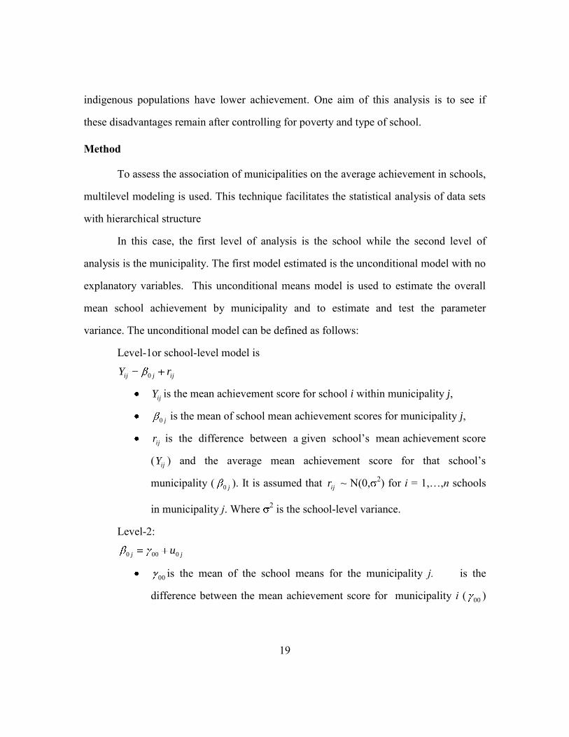
analysis is the municipality. The first model estimated is the unconditional model with no

explanatory variables. This unconditional means model is used to estimate the overall

mean school achievement by municipality and to estimate and test the parameter

variance. The unconditional model can be defined as follows:

Level-1or school-level model is

ijjij rY 0

ijY is the mean achievement score for school i within municipality j,

j0 is the mean of school mean achievement scores for municipality j,

ijr is the difference between a given school’s mean achievement score

( ijY ) and the average mean achievement score for that school’s

municipality ( j0 ). It is assumed that ijr ~ N(0,2) for i = 1,…,n schools

in municipality j. Where 2 is the school-level variance.

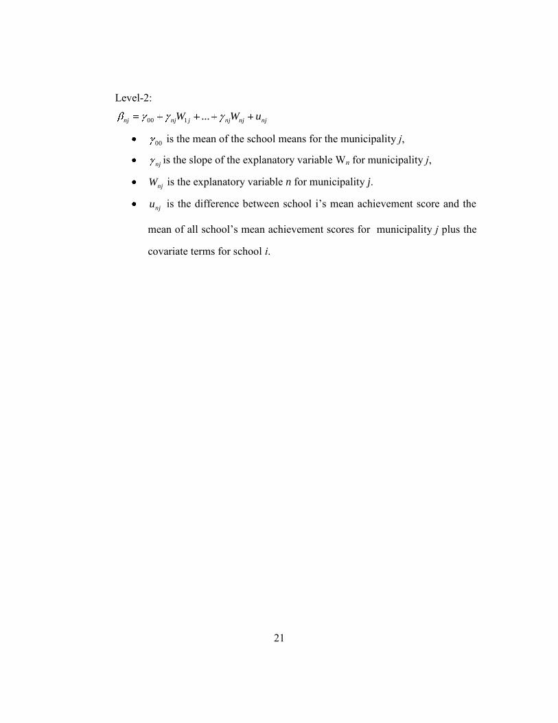
Level-2:

jj u0000

00 is the mean of the school means for the municipality j. is the

difference between the mean achievement score for municipality i ( 00 )

20

and the mean achievement for school i. It is assumed that ju0 ~ N(0, 00).

Where 00 is the municipality-level variance.

The unconditional model allows for an empirical confirmation of the need to use a

multilevel model. A multilevel model is needed if the variances of both levels differ

statistically from zero. Once the pertinence of multilevel modeling is confirmed by the

unconditional model, the conditional model can be stated.

The conditional model includes the explanatory variables and is used to estimate

and test the impact of the explanatory variables.

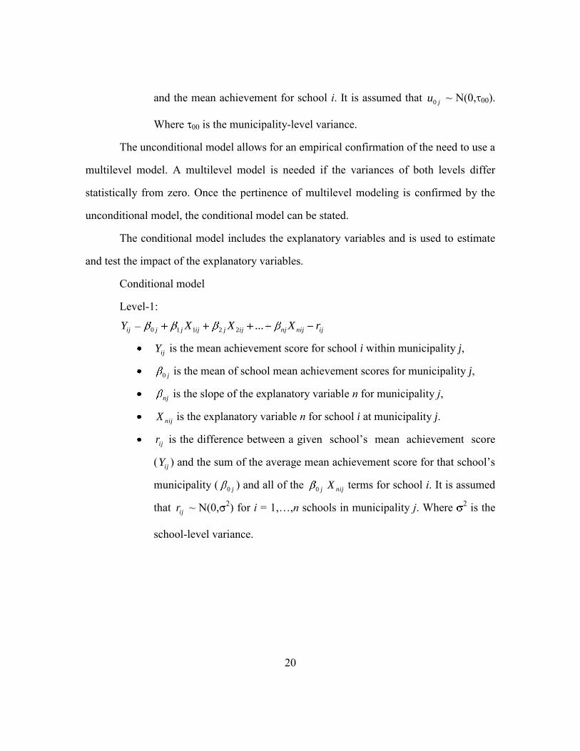
Conditional model

Level-1:

ijnijnjijjijjjij rXXXY ...22110

ijY is the mean achievement score for school i within municipality j,

j0 is the mean of school mean achievement scores for municipality j,

nj is the slope of the explanatory variable n for municipality j,

nijX is the explanatory variable n for school i at municipality j.

ijr is the difference between a given school’s mean achievement score

( ijY ) and the sum of the average mean achievement score for that school’s

municipality ( j0 ) and all of the j0 nijX terms for school i. It is assumed

that ijr ~ N(0,2) for i = 1,…,n schools in municipality j. Where

2 is the

school-level variance.

21

Level-2:

njnjnjjnjnj uWW ...100

00

is the mean of the school means for the municipality j,

nj is the slope of the explanatory variable Wn for municipality j,

njW is the explanatory variable n for municipality j.

nju is the difference between school i’s mean achievement score and the

mean of all school’s mean achievement scores for municipality j plus the

covariate terms for school i.

22

RESULTS

DESCRIPTIVE ANALYSIS

Table 5 shows the descriptive statistics for the school level variables. The mean

school math scores is 493.71, which falls below the national mean score of the students

(500). Around 12% of the schools are private schools, while 23% are general schools,

12% are technical schools, and 53% are telesecondary schools.

Table 5. Descriptive statistics for school level variables

Variable Mean Std. dev Minimum Maximum

Spanish mean score 481.92 63.08 279.99 797.17

Math mean score 493.71 61.36 321.53 823.21

Private 0.12 0.32 0.00 1.00

General 0.23 0.42 0.00 1.00

Technical 0.12 0.33 0.00 1.00

Telesecondary 0.53 0.50 0.00 1.00

School SES 317.00 1,155.64 0.00 74,829.17

Number of teachers 8.64 7.98 0.00 66.00

Number of teachers in CM 2.50 4.04 0.00 42.00

Teacher's average education (years) 15.61 0.77 3.00 20.00

Number of students 196.15 220.43 1.00 2,706.00

Morning shift 0.88 0.33 0.00 1.00

Dropout rate 7.89 8.57 0.00 95.70

Failure rate 11.93 13.07 0.00 93.30

With Oportunidades beneficiaries 0.85 0.36 0.00 1.00

Rural school 0.56 0.50 0.00 1.00

N 26,631

In this analysis, the number of teachers reflects the number of teachers actively

instructing students per school (as opposed to teachers performing administrative

functions). Here the mean number of teachers instructing students is almost 9. On

average, 2.5 teachers in each school were in the Carrera Magisterial Program, and the

average school has teachers who average 15.61 years of education

The average number of students is more than 196. 88% of the schools are in a

morning shift. The average dropout rate is 7.89%, and the average failure rate is almost

23

12%. 85% of the schools have at least one student who receives Oportunidades benefits,

and 56% of the schools are in rural areas.

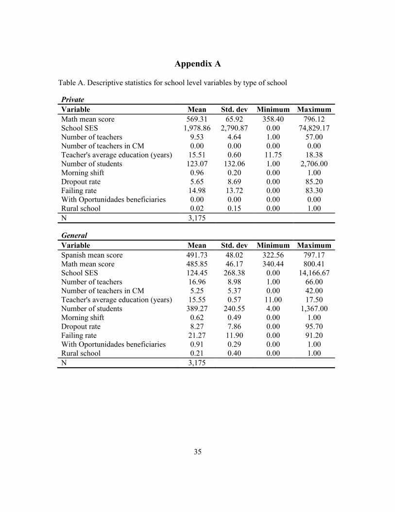
Appendix A shows the descriptive statistics by type of school. Private schools

have the higher mean math scores, with school means 83 points higher than general

schools. The differences by type of school demonstrate the importance of controling by

this variable. For instance, while general schools have on average 390 students,

telesecondaries have only 75, which is consistent with the fact that most of the general

secondary schools are located in urban areas whereas telesecondaries were designed to

serve populations in isolated areas. Accordingly, 90 percent of the telesecondaries are in

rural areas and only 27% of the technical, 21% of the general, and 2% of the private

schools belong to a rural community.

Regarding teachers’ education, the average number of years of schooling is very

similar for all types of school, but there are differences in standard deviation by type of

school. Teachers in telesecondaries average 15.68 years of education, slightly higher than

the national mean (15.61); however, their standard deviation is the highest (0.91) and the

average number of teachers is the lowest (3.52).

Table 6 shows the descriptive statistics for the municipality level variables. The

schools reported in the data set used in this work are distributed into 1,751 municipalities.

The average population size of these municipalities is 54,630 inhabitants but the variation

in this variable is large. There are communities with less than 250 inhabitants and

communities with more than 1.5 million people. On average, the number of communities

in these municipalities is almost 98 and the average number of rural communities by

municipality is 96.

24

Table 6. Descriptive statistics for municipality level variables


Population size 54,629.67 146,456.85 242.00 1,820,888.00

Number of communities 97.64 142.51 1.00 1,569.00

Number of rural communities 96.01 141.85 0.00 1,552.00

Communities with less than 100

inhabitants 72.26 125.46 0.00 1,447.00

Gini coefficient 0.425 0.04 0.26 0.69

IDH 0.763 0.07 0.47 0.95

Marginality index -0.200 0.97 -2.37 3.36

Proportion of indigenous population 0.137 0.265 0.000 0.999

N 1,751

The average Gini coefficient is 0.425, which is slightly lower than the Gini

coefficient at the national level in 2005 which was 0.501. This could be because the mean

reported here is an unweighted average.

The average HDI for the municipalities under study is 0.763, which is slightly

higher than the national HDI in 2005 (0.727). Again, this discrepancy could be due to the

unweighted averages used in this analysis.

The mean marginality index is equal to -0.2, which means that this group of

municipalities has a medium marginality level. However, the highest and lowest values of

the index show that there is large variation in level of marginality among the

municipalities under study, with some having very high levels of marginality and some

having very low levels of marginality. The proportion of indigenous population in these

municipalities varies from 0 to 0.999.

Two-level hierarchical linear models (Raudenbush and Bryk 2002) were

estimated using HLM 6.08 software to account for the nested nature of the data (i.e.,

schools within municipalities).

25

UNCONDITIONAL MODEL

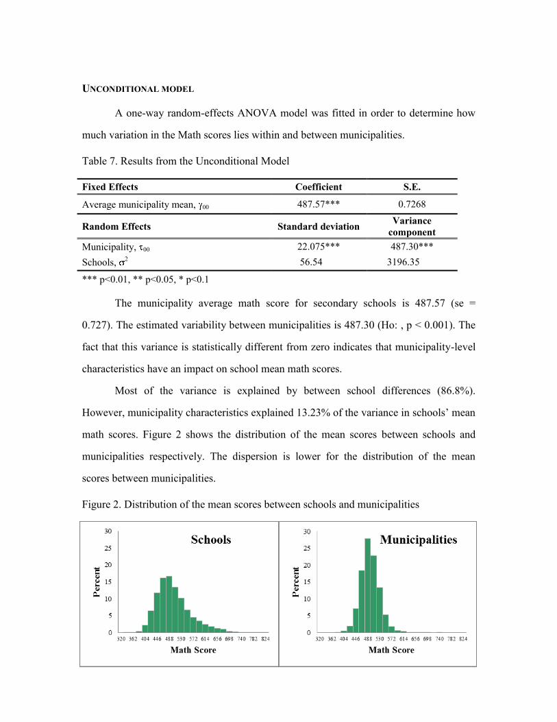
A one-way random-effects ANOVA model was fitted in order to determine how

much variation in the Math scores lies within and between municipalities.

Table 7. Results from the Unconditional Model

Fixed Effects Coefficient S.E.

Average municipality mean, 00 487.57*** 0.7268

Random Effects Standard deviation Variance

component

Municipality, 00 22.075*** 487.30***

Schools, 2 56.54*** 3196.35* **

*** p<0.01, ** p<0.05, * p<0.1

The municipality average math score for secondary schools is 487.57 (se =

0.727). The estimated variability between municipalities is 487.30 (Ho: , p < 0.001). The

fact that this variance is statistically different from zero indicates that municipality-level

characteristics have an impact on school mean math scores.

Most of the variance is explained by between school differences (86.8%).

However, municipality characteristics explained 13.23% of the variance in schools’ mean

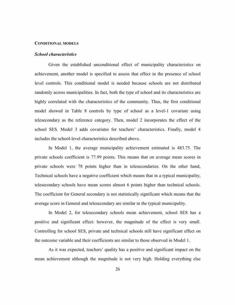
math scores. Figure 2 shows the distribution of the mean scores between schools and

municipalities respectively. The dispersion is lower for the distribution of the mean

scores between municipalities.

Figure 2. Distribution of the mean scores between schools and municipalities

26

CONDITIONAL MODELS

School characteristics

Given the established unconditional effect of municipality characteristics on

achievement, another model is specified to assess that effect in the presence of school

level controls. This conditional model is needed because schools are not distributed

randomly across municipalities. In fact, both the type of school and its characteristics are

highly correlated with the characteristics of the community. Thus, the first conditional

model showed in Table 8 controls by type of school as a level-1 covariate using

telesecondary as the reference category. Then, model 2 incorporates the effect of the

school SES. Model 3 adds covariates for teachers’ characteristics. Finally, model 4

includes the school-level characteristics described above.

In Model 1, the average municipality achievement estimated is 483.75. The

private schools coefficient is 77.99 points. This means that on average mean scores in

private schools were 78 points higher than in telesecondaries. On the other hand,

Technical schools have a negative coefficient which means that in a typical municipality,

telesecondary schools have mean scores almost 6 points higher than technical schools.

The coefficient for General secondary is not statistically significant which means that the

average score in General and telesecondary are similar in the typical municipality.

In Model 2, for telesecondary schools mean achievement, school SES has a

positive and significant effect: however, the magnitude of the effect is very small.

Controlling for school SES, private and technical schools still have significant effect on

the outcome variable and their coefficients are similar to those observed in Model 1.

As it was expected, teachers’ quality has a positive and significant impact on the

mean achievement although the magnitude is not very high. Holding everything else

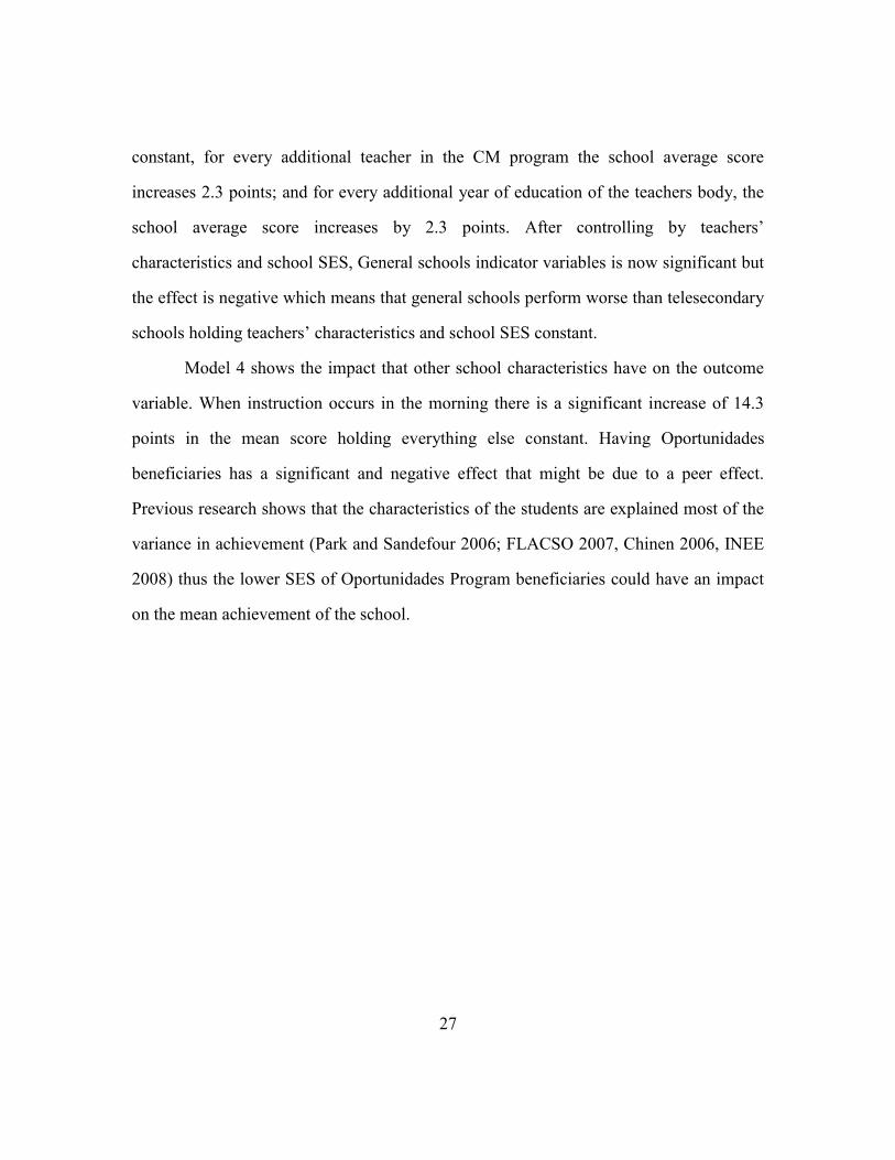
27

constant, for every additional teacher in the CM program the school average score

increases 2.3 points; and for every additional year of education of the teachers body, the

school average score increases by 2.3 points. After controlling by teachers’

characteristics and school SES, General schools indicator variables is now significant but

the effect is negative which means that general schools perform worse than telesecondary

schools holding teachers’ characteristics and school SES constant.

Model 4 shows the impact that other school characteristics have on the outcome

variable. When instruction occurs in the morning there is a significant increase of 14.3

points in the mean score holding everything else constant. Having Oportunidades

beneficiaries has a significant and negative effect that might be due to a peer effect.

Previous research shows that the characteristics of the students are explained most of the

variance in achievement (Park and Sandefour 2006; FLACSO 2007, Chinen 2006, INEE

2008) thus the lower SES of Oportunidades Program beneficiaries could have an impact

on the mean achievement of the school.

28

Table 8. Conditional models with school-level covariates

Fixed Effects Model 1 Model 2 Model 3 Model 4

Municipality mean achievement, 00 483.75*** 483.48*** 444.01*** 442.74***

(0.773) (0.779) (8.677) (9.065)

Private 77.99*** 72.38*** 78.01*** 66.66***

(1.198) (2.458) (2.455) (3.508)

General -1.06 -0.96 -13.20*** -12.07***

(1.064) (1.060) (1.366) (1.397)

Technical -5.88*** -5.84*** -18.42*** -22.43***

(1.281) (1.277) (1.352) (1.437)

School SES 0.003*** 0.003 ** 0.003 **

(0.001) (0.001) (0.001)

Number of teachers 0.40*** -0.152

(0.086) (0.098)

Number of teachers in CM 2.34*** 1.21***

(0.127) (0.139)

Teachers' education 2.27*** 2.20***

(0.551) (0.548)

Number of students 0.05***

(0.004)

Morning shift 14.29***

(1.075)

Dropout rate -0.123 **

(0.045)

Failing rate 0.026

(0.043)

With Oportunidades beneficiaries -13.04***

(2.747)

Rural school 1.672

(0.969)

Random Effects

Level-2 variance

Intercept 367.1683 367.2213 16865.24 16731.32

Teachers' education 68.04093 66.37076

Dropout rate 0.28277

Failing rate 0.30222

Level-1 variance

Schools, 2 2659.635 367.2213 2539.33 2419.793

Deviance 287098.1 287022.3 286131.7 285324.2

Parameters 2 2 4 11

*** p<0.01, ** p<0.05, * p<0.1

29

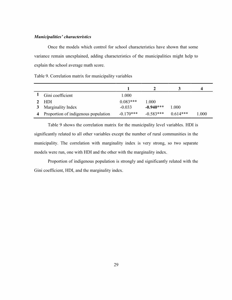
Municipalities’ characteristics

Once the models which control for school characteristics have shown that some

variance remain unexplained, adding characteristics of the municipalities might help to

explain the school average math score.

Table 9. Correlation matrix for municipality variables

1 2 3 4

1 Gini coefficient 1.000

2 HDI 0.083*** 1.000

3 Marginality Index -0.033 -0.940*** 1.000

4 Proportion of indigenous population -0.170*** -0.583*** 0.614*** 1.000

Table 9 shows the correlation matrix for the municipality level variables. HDI is

significantly related to all other variables except the number of rural communities in the

municipality. The correlation with marginality index is very strong, so two separate

models were run, one with HDI and the other with the marginality index.

Proportion of indigenous population is strongly and significantly related with the

Gini coefficient, HDI, and the marginality index.

30

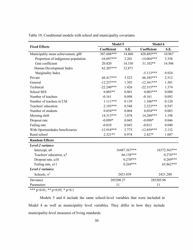
Table 10. Conditional models with school and municipality covariates

Fixed Effects Model 5 Model 6

Coefficient S.E. Coefficient S.E.

Municipality mean achievement, g00 387.688*** 14.460 428.885*** 10.967

Proportion of indigenous population -16.697*** 3.201 -14.064*** 3.358

Gini coefficient 20.820*** 14.330 31.102*** 14.506

Human Development Index 62.207*** 12.871

Marginality Index -5.113*** 0.924

Private 66.417*** 3.523 66.385*** 2.512

General -12.237*** 1.392 -12.361*** 1.301

Technical -22.240*** 1.426 -22.315*** 1.374

School SES 0.003*** 0.001 0.003*** 0.000

Number of teachers -0.161*** 0.098 -0.161*** 0.093

Number of teachers in CM 1.111*** 0.139 1.106*** 0.120

Teachers' education 2.193*** 0.548 2.223*** 0.547

Number of students 0.054*** 0.004 0.054*** 0.003

Morning shift 14.313*** 1.078 14.289*** 1.198

Dropout rate -0.099*** 0.045 -0.098*** 0.046

Failing rate -0.010*** 0.043 -0.013*** 0.040

With Oportunidades beneficiaries -12.918*** 2.775 -12.859*** 2.132

Rural school 2.321*** 0.974 2.427*** 1.087

Random Effects

Level-2 variance

Intercept, u0 16487.367*** 16372.563***

Teachers' education, u7 66.138*** 0.274***

Dropout rate, u10 0.270*** 0.269***

Failing rate, u11 0.269*** 65.862***

Level-1 variance

Schools, 2 2421.039*** 2421.280***

Deviance 285208.27 285205.96

Parameters 11 11

*** p<0.01, ** p<0.05, * p<0.1

Models 5 and 6 include the same school-level variables that were included in

Model 4 as well as municipality level variables. They differ in how they include

municipality-level measures of living standards.

31

Model 5 uses HDI to control for living standards in the municipality. HDI has a

positive and significant effect on the overall intercept ( 00). That means that better living

conditions (higher HDI) yield to a better average achievement in math, holding

everything else constant. Proportion of indigenous population has also a significant effect

on achievement. On the other hand, Model 6 includes marginality index instead of HDI,

the coefficient is also significant but in this case the effect is negative, as it was expected,

and the magnitude is much lower. In sum, these two models indicate that better living

conditions are associated with higher mean test scores even after controlling for school

factors.

The Gini coefficient effect is not significant in model 5 but it becomes significant

when HDI is substituted for the marginality index. This could be due to the fact that the

correlation between HDI and Gini coefficient is significant while the correlation between

marginality index and Gini coefficient is not. The effect of the Gini coefficient is positive

which means that higher inequality is associated with higher overall mean test scores, net

of covariates.

The proportion of indigenous population, as it was expected, has a negative and

significant effect in Model 5 and 6. The magnitude of the coefficients of this variable is

very similar in both models. On average, a one unit increase in the proportion of

indigenous population the municipality is associated with a decrease in mean

achievement ( 00) of 16.6 points (Model 5, or 14.1 in Model 6) holding everything else

constant.

To test the third hypothesis, an intercepts – and slopes – as – outcome model

(Raudenbush and Bryk 2002) is presented in Table 11. In this model, the municipality

level variables are used to model the intercept and the slope of teachers’ education and

dropout rate, because these variables are assumed to be random factors. Failure rate is

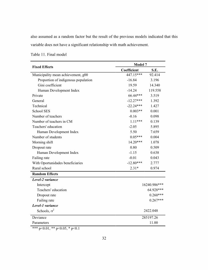
32

also assumed as a random factor but the result of the previous models indicated that this

variable does not have a significant relationship with math achievement.

Table 11. Final model

Fixed Effects Model 7

Coefficient S.E.

Municipality mean achievement, g00 447.15*** 92.414

Proportion of indigenous population -16.84*** 3.196

Gini coefficient 19.59*** 14.340

Human Development Index -14.24*** 119.558

Private 66.44*** 3.519

General -12.27*** 1.392

Technical -22.24*** 1.427

School SES 0.003** 0.001

Number of teachers -0.16*** 0.098

Number of teachers in CM 1.11*** 0.139

Teachers' education -2.05*** 5.895

Human Development Index 5.50*** 7.659

Number of students 0.05*** 0.004

Morning shift 14.20*** 1.078

Dropout rate 0.80*** 0.509

Human Development Index -1.15*** 0.638

Failing rate -0.01*** 0.043

With Oportunidades beneficiaries -12.80*** 2.777

Rural school 2.31*** 0.974

Random Effects

Level-2 variance

Intercept 16240.986***

Teachers' education 64.928***

Dropout rate 0.260***

Failing rate 0.267***

Level-1 variance

Schools, 2 2422.048***

Deviance 285197.26***

Parameters 11.00***

*** p<0.01, ** p<0.05, * p<0.1

33

The results do not provide evidence of a significant relationship between HDI and

the effect of dropout rate on mean scores or between HDI and the effect of teachers’

education on mean scores. The rest of the coefficients are similar to those in model 5.

In light of these findings, it cannot be concluded that places with higher living

standards benefit more from better prepared teachers or more committed students.

However, there is evidence that those municipalities with higher living standards do have

higher average math scores and that the influence of beneficial and detrimental impacts

on these scores is consistent across levels of human development.

CONCLUSION

Previous research has demonstrated that characteristics of schools better explain

mean student outcomes than do characteristics of municipalities. However, substantial

variability in mean student outcomes remains unexplained after accounting for

characteristics of schools. Some of this unexplained variability could be due to

unmeasured heterogeneity at the student level (Park and Sandefour 2006; FLACSO 2007,

Chinen 2006, INEE 2008). The present work demonstrates that, while school-level

characteristics are important, municipality characteristics provide additional explanation

of this unexplained variability even without accounting for student characteristics.

Although the municipality factors explain only 13% of the total variance of the school

average score in Math, the models presented provide evidence to support the hypothesis

that municipalities vary in their school mean math scores.

The municipality-level variables are highly correlated, and thus each of their

individual impacts of school mean test scores is not as strong as was expected, yet there

is evidence that municipality-level characteristics do impact school average achievement.

34

The Human Development Index is the municipality-level variable with the

strongest effect on the outcome variable. The effect of the HDI supports the hypothesis

that schools in more developed municipalities have an advantage over schools in less

developed areas.

In sum, it can be said that municipality factors are important for achievement

outcomes although their effect is not outstanding mainly because as other studies

conclude individual-level variables have the strongest effect.

LIMITATIONS

In 2006, ENLACE was not applied in Michoacán and Oaxaca because local

teachers’ union refuse to be evaluated in Michoacán and teachers were on strike in

Oaxaca. The effect of municipality in these states may differ due to the power of local

teachers’ union. It is also possible that schools performance is worse than the country

average.

35

Appendix A

Table A. Descriptive statistics for school level variables by type of school

Private


Math mean score 569.31 65.92 358.40 796.12

School SES 1,978.86 2,790.87 0.00 74,829.17





Morning shift 0.96 0.20 0.00 1.00

Dropout rate 5.65 8.69 0.00 85.20

Failing rate 14.98 13.72 0.00 83.30


Rural school 0.02 0.15 0.00 1.00

N 3,175

General



Math mean score 485.85 46.17 340.44 800.41

School SES 124.45 268.38 0.00 14,166.67





Morning shift 0.62 0.49 0.00 1.00

Dropout rate 8.27 7.86 0.00 95.70

Failing rate 21.27 11.90 0.00 91.20


Rural school 0.21 0.40 0.00 1.00

N 3,175

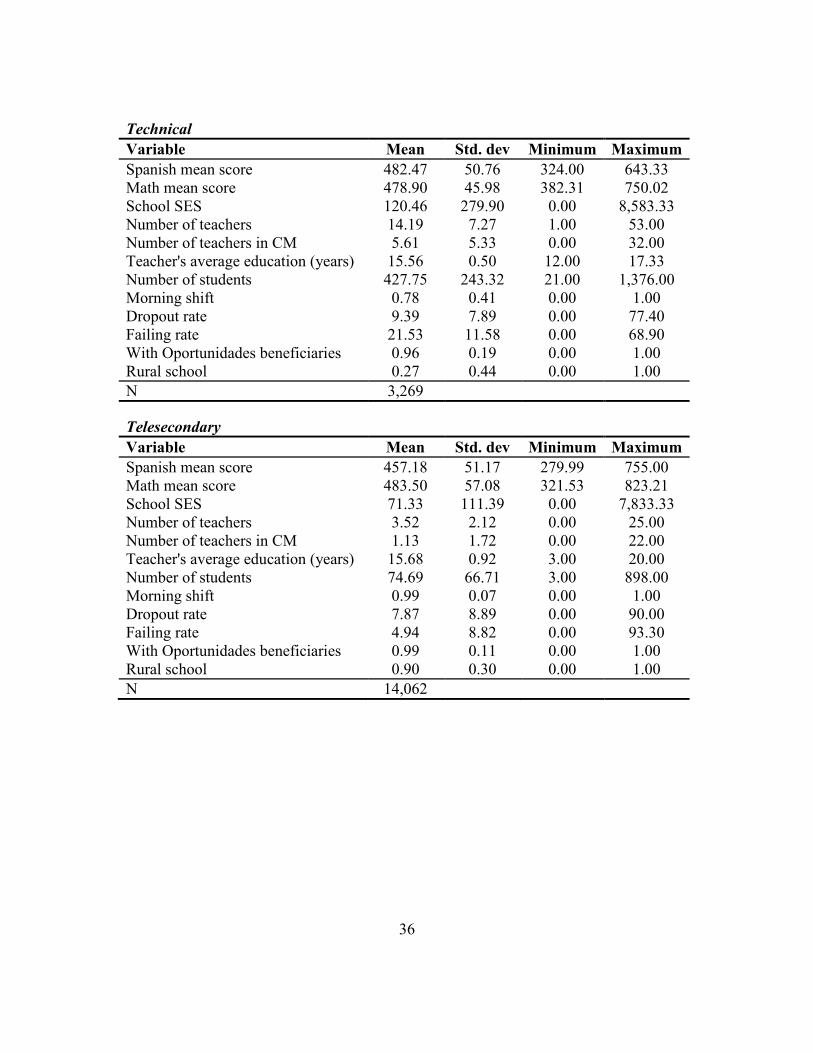
36

Technical



Math mean score 478.90 45.98 382.31 750.02

School SES 120.46 279.90 0.00 8,583.33





Morning shift 0.78 0.41 0.00 1.00

Dropout rate 9.39 7.89 0.00 77.40

Failing rate 21.53 11.58 0.00 68.90


Rural school 0.27 0.44 0.00 1.00

N 3,269

Telesecondary



Math mean score 483.50 57.08 321.53 823.21

School SES 71.33 111.39 0.00 7,833.33




Number of students 74.69 66.71 3.00 898.00

Morning shift 0.99 0.07 0.00 1.00

Dropout rate 7.87 8.89 0.00 90.00

Failing rate 4.94 8.82 0.00 93.30


Rural school 0.90 0.30 0.00 1.00

N 14,062

37

References

Baker, David P., Brian Goesling, and Gerald K. Letendre. 2002. "Socioeconomic Status,

School Quality, and National Economic Development: A Cross-National Analysis

of the "Heyneman-Loxley Effect" on Mathematics and Science Achievement."

Comparative Education Review 46:291-312.

Bännström, Lars. 2008. "Making Their Mark: The Effects of Neighborhood and Upper

Secondary School on Educational Achievement." European Sociological Review

24:463-478.

Battistich, V., Solomon, D., Kim, D.-i., Watson, M., & Schaps, E. (1995). Schools as

Communities, Poverty Levels of Student Populations, and Students' Attitudes,

Motives, and Performance: A Multilevel Analysis. American Educational

Research Journal, 32(3), 627-658.

Buchmann, Claudia and Emily Hannum. 2001. ―Education and Stratification in

Developing Countries: A Review of Theories and Research.‖ Annual Review of

Sociology 27:77-102.

Buchmann, Claudia. 2002. ―Getting Ahead in Kenya: Social Capital, Shadow Education

and Achievement.‖ Research in Sociology of Education 133-59.

Chinen, Marjorie. 2006. ―Análisis de los Resultados de la Prueba Nacional de

Arovechamiento en Lectura en Secundaria: Estudio Multinivel de Logro y

Tendencias.‖ Mexico: INEE

Comité Técnico para la Medición de la Pobreza (CTMP). 2002. ―Medición de la pobreza:

variantes metodológicas y estimación preliminar.‖ Secretaría de Desarrollo

Social. México D.F.

Consejo Nacional de Evaluación de la Política de Desarrollo Social (CONEVAL). 2007.

―Los Mapas de Pobreza en México‖. CONEVAL.

Consejo Nacional de Población (CONAPO). 2005. ―Proyecciones de Población indígena,

2000-2010‖. Retrieved July 23, 2008 (http://www.conapo.gob.mx/index.php?

option=com_content &view=article&id=37&Itemid=235).

______. 2007. ―Índice de marginación a nivel localidad 2005‖. CONAPO.

Epstein, J. and M. Sanders. 2000. ―Connecting home, school, and community: new

directions for social research.‖ In M. Hallinan. Handbook of the Sociology of

Education. Springer.

Evaluation of the Latin American Laboratory for the Evaluation of Educational Quality

(LLECE). 2001. ―Segundo Informe de Resultados. Primer Estudio Internacional

Comparativo sobre lenguaje, matemática y factores asociados, para alumnos del

tercer y cuarto grado de la educación básica‖. UNESCO-OREALC.

38

Facultad Latinoamericana de Ciencias Sociales (FLACSO). 2007. ―Factores asociados al

logro educativo de matemáticas y español en la Prueba ENLACE 2007: un

análisis multinivel.‖ FLACSO.

Gutiérrez, Edith Y. 2010. ―El Espacio Como Eje de Análisis de la Desigualdad Educativa

en el México del Siglo XXI.‖ Master Thesis, Centro de Estudios Urbanos,

Demográficos y Ambientales. Colegio de México, México, D.F.

Gutiérrez, Edith Y, Silvia Giorguli, and Landy Sánchez. 2010. ―The Spatial Dimension of

Educational Inequality in Mexico in the Beginning of the Twenty-First Century.‖

Presented at the annual meeting of the Population Association of America, April

15, Dallas, TX.

Instituto Nacional de Estadística y Geografía (INEGI). 2005a. ―Conteo de Población y

Vivienda 2005. Tabulados Básicos.‖ Retrieved February 5, 2011 (http://

www.inegi.org.mx/ sistemas/TabuladosBasicos/Default.aspx?c=10398&s=est).

_____. 2005b. ―Conteo de Población y Vivienda 2005. Consulta Interactiva de datos.‖

Retrieved February 5, 2011 (http:// www.inegi.org.mx /sistemas/olap /proyectos/

bd/consulta.asp?p=10215&c=16851&s=est#).

Instituto Nacional para la Evaluación de la Educación (INEE). 2006. ―Panorama

Educativo de México 2006 Indicadores del Sistema Educativo Nacional‖. INEE.

______. 2008. ―Análisis multinivel de la calidad educativo en México ante los datos de

PISA 2006‖. INEE.

Jimenez, Emmanuel and Yasuyuki Sawada. 1999. "Do Community-Managed Schools

Work? An Evaluation of El Salvador's EDUCO Program." The World Bank

Economic Review 13:415-441.

Ley General de Educación. 1993. Diario Oficial de la Federación. July 13th

, 1993

Lubienski, S. T., & Lubienski, C. 2006. School Sector and Academic Achievement: A

Multilevel Analysis of NAEP Mathematics Data. American Educational Research

Journal, 43(4), 651-698.

OECD 2010, "Aggregate National Accounts: Gross domestic product", OECD National

Accounts Statistics (database). Retrieved March 28, 2011. (http://stats.oecd.org/

BrandedView.aspx?oecd_bv_id=na-data-en&doi=data-00001-en)

Park, Hyunjoon and Gary D. Sandefur. 2006. "Families, Schools, and Reading in Asia

and Latin America." Research in the Sociology of Education 15:133-162.

Programa de Desarrollo Humano Oportunidades (Oportunidades). 2010. ―Estudio

Complementario Sobre la Calidad de los Servicios Educativos que Ofrece el

Programa a su Población Beneficiaria Rural.‖ Oportunidades.

Programa de las Naciones Unidas para el Desarrollo (UNDP). 2008. ―Índice de

Desarrollo Humano Municipal en México 2000-2005.‖ UNDP.

39

Raudenbush, S. W., & Bryk, A. S. 2002. Hierarchical linear models: Applications and

data analysis methods. Newbury Park, CA: Sage Publications, Inc.

Salinas, Viviana and Joseph Potter. 2008. ―Cambio Demográfico y Oportunidades

Educativas en México, Brasil, y Chile.‖ Presented at the III Meeting of the Latin

American Population Association. September 24, Córdoba, Argentina.

Santibañez, L., Martínez, J. F., Datar, A., McEwan, P. J., Setodji, C. M., and Basurto-

Dávila, R. (2007) Breaking Ground: Analysis of the assessments and impact of

the Carrera Magisterial program in Mexico. Santa Monica, CA: RAND/MG-141

(also available in Spanish)

Santibañez, Lucrecia. 2008. ―El Impacto del Gasto Sobre la Calidad Educativa.‖ in

Estudios sobre Desarrollo Humano, vol. 2009-9. Mexico: UNPD.

Secretaría de Educación Pública (SEP). 2007. ―Sistema Educativo de los Estados Unidos

Mexicanos. Principales Cifras. Ciclo Escolar 2005-2006.‖ SEP.

UNESCO and United Nations Committee on Economic, Social and Cultural Rights.

1999. Right to Education: Scope and Implementation.

Villegas-Reimers, E., y Reimers, F. (1996). Where are 60 million teachers? The missing

voice in educational reforms around the world. Prospects, vol. XXVI, no. 3,

September.

Yúnez, A., Arellano, J. y Méndez, J. 2009. ―México: Consumo, pobreza y desigualdad a

nivel municipal. 1990-2005‖. Documento de Trabajo N° 31. Programa Dinámicas

Territoriales Rurales. Rimisp, Santiago, Chile.

copyright by celia hubert lopez 2011

Documents