copyright by mahdy shirdel 2013
TRANSCRIPT

Copyright
by
Mahdy Shirdel
2013

The Dissertation Committee for Mahdy Shirdel
Certifies that this is the approved version of the following dissertation:
Development of a Coupled Wellbore-Reservoir Compositional
Simulator for Damage Prediction and Remediation
Committee:
Kamy Sepehrnoori, Supervisor
Gary A. Pope
Kishore Mohanty
Mojdeh Delshad
Dale D. Erickson

Development of a Coupled Wellbore-Reservoir Compositional
Simulator for Damage Prediction and Remediation
by
Mahdy Shirdel, B.M.E, M.S.E.
Dissertation
Presented to the Faculty of the Graduate School of
The University of Texas at Austin
in Partial Fulfillment
of the Requirements
for the Degree of
Doctor of Philosophy
The University of Texas at Austin
August 2013

To
my wife
Sahar
without her support none of this would be possible

v
Acknowledgments
I would like to express my sincere gratitude to my supervising professor, Dr. Kamy
Sepehrnoori, for his continuous guidance, support, and encouragement. I have learned a
lot from his profound insight, keen observations, and vast knowledge. I am privileged to
have had an opportunity to work with him.
I appreciate the time, valuable comments, and feedback of my committee
members, Dr. Gary A. Pope, Dr. Mojdeh Delshad, Dr. Kishore Mohanty, and Dr. Dale
Erickson. Special thanks go to Dr. Chowdhury Mamun for review and comments in my
dissertation.
I would like to acknowledge the staff of the Petroleum and Geosystems
Engineering Department at The University of Texas at Austin, Dr. Roger Terzian,
Michelle Mason, Joanna Castillo, Cheryl Kruzie, Frankie Hart, and Mary Pettengill for
their technical and administrative support.
Special thanks to my friends Abolghasem (Abe) Kazeminia, Hamed Darabi and
Saeedeh Mohebbinia for their indispensable help and knowledge sharing about
PHREEQC, UTCOMP and Asphaltene phase behavior modeling, Victor Magri and Ali
Abouei for their valuable technical discussions and help in providing the user’s manual
and technical guide for UTWELL. I also enjoyed technical discussions with Dr. Walter
Fair, Dr. Abdoljalil Varavei, Dr. Mohammad H. Kalaei and Dr. Paulo Ribeiro.
I sincerely thank the financial support provided by Abu Dhabi National Oil
Company and Reservoir Simulation JIP at the Center for Petroleum and Geosystem
Engineering Department at The University of Texas at Austin.
August 2013

vi
Abstract
Development of a Coupled Wellbore-Reservoir Compositional
Simulator for Damage Prediction and Remediation
Mahdy Shirdel, Ph.D.
The University of Texas at Austin, 2013
Supervisor: Kamy Sepehrnoori
During the production and transportation of oil and gas, flow assurance issues
may occur due to the solid deposits that are formed and carried by the flowing fluid.
Solid deposition may cause serious damage and possible failure to production equipment
in the flow lines. The major flow assurance problems that are faced in the fields are
concerned with asphaltene, wax and scale deposition, as well as hydrate formations.
Hydrates, wax and asphaltene deposition are mostly addressed in deep-water
environments, where fluid flows through a long path with a wide range of pressure and
temperature variations (Hydrates are generated at high pressure and low temperature
conditions). In fact, a large change in the thermodynamic condition of the fluid yields
phase instability and triggers solid deposit formations. In contrast, scales are formed in
aqueous phase when some incompatible ions are mixed.

vii
Among the different flow assurance issues in hydrocarbon reservoirs, asphaltenes
are the most complicated one. In fact, the difference in the nature of these molecules with
respect to other hydrocarbon components makes this distinction. Asphaltene molecules
are the heaviest and the most polar compounds in the crude oils, being insoluble in light
n-alkenes and readily soluble in aromatic solvents. Asphaltene is attached to similarly
structured molecules, resins, to become stable in the crude oils. Changing the crude oil
composition and increasing the light component fractions destabilize asphaltene
molecules. For instance, in some field situations, CO2 flooding for the purpose of
enhanced oil recovery destabilizes asphaltene. Other potential parameters that promote
asphaltene precipitation in the crude oil streams are significant pressure and temperature
variation.
In fact, in such situations the entrainment of solid particulates in the flowing fluid
and deposition on different zones of the flow line yields serious operational challenges
and an overall decrease in production efficiency. The loss of productivity leads to a large
number of costly remediation work during a well life cycle. In some cases up to $5
Million per year is the estimated cost of removing the blockage plus the production losses
during downtimes. Furthermore, some of the oil and gas fields may be left abandoned
prematurely, because of the significance of the damage which may cause loss about $100
Million.
In this dissertation, we developed a robust wellbore model which is coupled to our
in-house developed compositional reservoir model (UTCOMP). The coupled
wellbore/reservoir simulator can address flow restrictions in the wellbore as well as the
near-wellbore area. This simulator can be a tool not only to diagnose the potential flow
assurance problems in the developments of new fields, but also as a tool to study and
design an optimum solution for the reservoir development with different types of flow

viii
assurance problems. In addition, the predictive capability of this simulator can prescribe a
production schedule for the wells that can never survive from flow assurance problems.
In our wellbore simulator, different numerical methods such as, semi-implicit,
nearly implicit, and fully implicit schemes along with blackoil and Equation-of-State
compositional models are considered. The Equation-of-State is used as state relations for
updating the properties and the equilibrium calculation among all the phases (oil, gas,
wax, asphaltene). To handle the aqueous phase reaction for possible scales formation in
the wellbore a geochemical software package (PHREEQC) is coupled to our simulator as
well.
The governing equations for the wellbore/reservoir model comprise mass
conservation of each phase and each component, momentum conservation of liquid, and
gas phase, energy conservation of mixture of fluids and fugacity equations between three
phases and wax or asphaltene. The governing equations are solved using finite difference
discretization methods.
Our simulation results show that scale deposition is mostly initiated from the
bottom of the wellbore and near-wellbore where it can extend to the upper part of the
well, asphaltene deposition can start in the middle of the well and the wax deposition
begins in the colder part of the well near the wellhead. In addition, our simulation studies
show that asphaltene deposition is significantly affected by CO2 and the location of
deposition is changed to the lower part of the well in the presence of CO2.
Finally, we applied the developed model for the mechanical remediation and
prevention procedures and our simulation results reveal that there is a possibility to
reduce the asphaltene deposition in the wellbore by adjusting the well operation
condition.

ix
Table of Contents
List of Tables ....................................................................................................xv
List of Figures............................................................................................... xviii
Chapter 1: Introduction ................................................................................... 1
1.1 Description of the Problem................................................................. 1
1.2 Research Objectives........................................................................... 3
1.3 Brief Description of the Chapters ....................................................... 4
Chapter 2: Background and Literature Review.............................................. 6
2.1 Multiphase Flow Modeling in Wellbores............................................ 6
2.2 Asphaltene and Wax Precipitation.................................................... 13
2.3 Geochemical Scale Formation.......................................................... 17
2.4 Asphaltene and Scale Deposition Models in Wellbores .................... 18
2.5 Wax Deposition Models in Wellbores .............................................. 21
Chapter 3: Multiphase Flow Models in the Wellbores and Pipelines........... 23
3.1 Single Phase Flow Equations ........................................................... 23
3.2 Multiphase Flow Equations.............................................................. 24
3.2.1 Mass Conservation Equations.................................................. 26
3.2.2 Momentum Conservation Equation with Homogenous Approach ....................................................................................... 28
3.2.3 Momentum Conservation Equation with Drift-flux Approach.. 30
3.2.4 Momentum Conservation Equations with Two-fluid Approach ... ....................................................................................... 31
3.3 Eigenvalue Analysis of Multiphase Flow Equations ......................... 36
3.3.1 Mathematical Stability of IVP, Ill-Posed Problems .................. 37
3.3.2 Characteristic Roots of Multiphase Flow Equations................. 38
3.4 Regularization of non-Hyperbolic Equations .................................... 44
3.5 Flow Regime Detection.................................................................... 46
3.5.1 Flow Patterns in Vertical and Deviated Wells .......................... 47
3.5.2 Flow Patterns in Horizontal Wells ........................................... 55

x
3.6 Constitutive Relations ...................................................................... 58
3.6.1 Drift-flux Model...................................................................... 59
3.6.2 Two-fluid Model ..................................................................... 61
3.7 Phasic Wall Friction......................................................................... 63
3.8 Interphase Mass Transfer ................................................................. 65
3.9 State Relations ................................................................................. 65
Chapter 4: Wellbore Heat Transfer Models ................................................. 73
4.1 Energy Equation in the Wellbore...................................................... 73
4.2 Wellbore Heat Loss Model............................................................... 75
4.3 Ambient Temperature Model ........................................................... 75
Chapter 5: Wellbore Models Numerical Solutions ....................................... 86
5.1 Discretization of Field Equations ..................................................... 86
5.1.1 Discretization Method for Two-fluid Models........................... 87
5.1.2 Discretization Method for Drift-flux Model............................. 95
5.2 Wellbore Boundary Conditions ........................................................ 98
5.3 Solution Methods............................................................................. 99
5.3.1 Semi-Implicit Approach .........................................................100
5.3.2 Nearly-Implicit Approach.......................................................105
5.3.3 Fully-Implicit Approach .........................................................108
5.3.4 Steady State Model.................................................................110
5.3.5 Updating the State Relations...................................................113
5.4 Time-Step Control ..........................................................................114
5.5 Numerical Convergence and Robustness of Solutions .....................116
5.5.1 Water Faucet Problem ............................................................116
5.5.2 Phase Redistribution Problem.................................................118
5.6 Simulation Results ..........................................................................119
5.6.1 Comparison of Different Numerical Methods .........................120
5.6.1.1 Three-phase Flow Simulation......................................120
5.6.1.2 Gas Production Simulation..........................................122
5.6.2 Validation of Transient Models ..............................................123

xi
5.6.3 Validation of Steady State Models..........................................123
5.6.3.1 Gas-lift Simulation ...................................................123
5.6.3.2 Wellbore Temperature Model...................................124
Chapter 6: Flow Assurance Issues in the Wellbore......................................140
6.1 Asphaltene ......................................................................................140
6.1.1 Asphaltene Precipitation Model..............................................141
6.1.2 Asphaltene Aggregation .........................................................146
6.1.3 Verification of Asphaltene Precipitation Model ......................148
6.2 Wax ................................................................................................149
6.2.1 Wax Precipitation Model........................................................150
6.2.2 Verification of Wax Precipitation Model ................................154
6.3 Geochemical Scale ..........................................................................155
6.3.1 Scale Precipitation Model.......................................................158
Chapter 7: Particle Deposition in the Flow Stream .....................................168
7.1 Asphaltene and Scale Deposition Models ........................................168
7.1.1 Terminology...........................................................................171
7.1.2 Deposition Mechanisms .........................................................173
7.1.3 Friedlander and Johnstone Model ...........................................174
7.1.4 Beal Model.............................................................................177
7.1.5 Escobedo and Mansoori Model...............................................179
7.1.6 Cleaver and Yates Model .......................................................183
7.2 Asphaltene and Scale Deposition Model in Laminar Flow...............184
7.3 Attachment Process.........................................................................186
7.4 Comparison of Deposition Models with Experimental Results ........188
7.4.1 Gas/Iron Flow Experiment with no Re-entrainment ................188
7.4.2 Oil/Asphaltene Flow Experiment............................................189
7.5 Wax Deposition Models..................................................................191
Chapter 8: Particle Transportation in Multiphase Flow .............................204
8.1 Deposition Kinetics in Multiphase Flow Systems............................204
8.2 Particle Mass Conservation Equation ..............................................205

xii
8.3 Simulations Results in Stand-alone Wellbore Model .......................208
8.4 Asphaltene Deposition ....................................................................208
8.4.1 Asphaltene Deposition Case Study with Fluid Sample 1 .........209
8.4.2 Effect of CO2 on Asphaltene Deposition.................................211
8.4.3 Asphaltene Deposition Case Study with Fluid Sample 2 .........213
8.5 Wax Deposition ..............................................................................214
8.6 Scale Deposition .............................................................................214
Chapter 9: Coupled Wellbore Reservoir Model...........................................236
9.1 A Review of Coupled Wellbore Reservoir Models ..........................237
9.2 Methods of Coupling Wellbore to the Reservoir..............................239
9.3 Coupled Wellbore / Reservoir Model Results ..................................241
9.3.1 Asphaltene Deposition Case One............................................242
9.3.2 Asphaltene Deposition Case Two ...........................................243
Chapter 10: Remediation and Prevention Procedures for Asphaltene Deposition................................................................................................................255
10.1 Asphaltene Deposition Prevention Procedures.................................255
10.2 Asphaltene Deposition Remediation Procedures..............................256
10.3 Simulation Studies ..........................................................................258
10.3.1 Effect of Wellhead Pressure..................................................258
10.3.2 Effect of Tubing Size............................................................259
10.3.3 Effect of Wellbore Heat Transfer Coefficient........................260
Chapter 11: Summary, Conclusions and Recommendations.......................267
11.1 Summary ........................................................................................267
11.2 Conclusions ....................................................................................269
11.3 Recommendations...........................................................................272
Appendix A : Reservoir Simulation Model (UTCOMP)...............................277
A.1 Reservoir Governing Equations.......................................................278
A.1.1 Volume Constraint .................................................................279
A.1.2 Pressure Equation...................................................................279
A.1.3 Overall Computational Procedure of UTCOMP......................280

xiii
A.2 Well Model.....................................................................................281
A.2.1 Constant Flowing Bottom-hole Pressure Injector....................284
A.2.2 Constant Molar Rate Injector..................................................285
A.2.3 Constant Volume Rate Injector...............................................287
A.2.4 Constant Molar Rate Production Well ....................................287
A.2.5 Constant Flowing Bottom-hole Pressure Producer ..................289
A.2.6 Constant Volume Oil Rate Producer.......................................289
A.2.7 Constant Wellhead Pressure Producer/Injector .......................290
Appendix B: Compositional PVT Models .....................................................291
B.1 Compressibility Factor ....................................................................291
B.2 Phase Equilibrium...........................................................................293
B.3 Density ...........................................................................................294
B.4 Viscosity.........................................................................................295
B.5 Enthalpy .........................................................................................296
B.6 Interfacial Tension ..........................................................................298
Appendix C: Black Oil PVT Models..............................................................301
C.1 Gas Compressibility Factor .............................................................301
C.2 Density ...........................................................................................302
C.3 Viscosity.........................................................................................304
C.4 Enthalpy .........................................................................................305
C.5 Interfacial Tension ..........................................................................307
Appendix D: Derivation of Balance Equations .............................................308
D.1 General Balance Equations in Single-phase Flow............................308
D.2 General Balance Equations in Multiphase Flow ..............................310
D.3 Basic Assumptions..........................................................................314
Appendix E : Unit Conversions .....................................................................317
Appendix F: UTWELL Keywords.................................................................318
F.1 Flow Path Definition and Trajectory ...............................................318
F.2 Fluid Property .................................................................................320

xiv
F.3 Process Condition ...........................................................................325
F.4 Initial Condition..............................................................................326
F.5 Boundary Condition........................................................................327
F.6 Output Options................................................................................328
F.7 Numerical Options ..........................................................................328
Appendix G: Sample Input Data ...................................................................330
G.1 Transient Three Phase Flow Simulation .........................................330
G.2 Standalone Asphaltene Deposition Simulation ................................333
G.3 Standalone Wax Deposition Simulation .........................................337
G.4 Standalone Geochemical Scale Deposition Simulation ...................340
G.5 Coupled Wellbore/Reservoir Simulation .........................................343
G.6 PHREEQC Sample Database ..........................................................353
G.7 PHREEQC Sample Input Data ........................................................356
Glossary ..........................................................................................................358
References.......................................................................................................361
Vita ................................................................................................................375

xv
List of Tables
Table 4.1 Wellbore and formation geometry ................................................. 83
Table 5.1 Input parameters for gas/oil/ water three-phase flow simulation in
UTWELL with different numerical schemes ................................126
Table 5.2 Input parameters for gas/water two-phase flow simulation in UTWELL
and OLGA ...................................................................................126
Table 5.3 Input parameters for the gas-lift simulation in UTWELL and PIPESIM
....................................................................................................127
Table 5.4 Input parameters for comparison of wellbore temperature calculation
between UTWELL, PIPESIM and analytical model from Hasan and
Kabir (1996) ................................................................................127
Table 5.5 Comparison of computation times for different numerical models on a
windows platform with 2.17 GB usable RAM and 2.30 GHz CPU128
Table 6.1 Fluid characterization and composition for comparing the model against
Burke, et al. (1990) ......................................................................162
experimental data .............................................................................................162
Table 6.2 Binary interaction coefficients used for modeling Burke et al. (1990)
fluid .............................................................................................162
Table 6.3 Molar composition of Oil 11a – Oil 11f from Rønningsen et al. (1997)
experimental data for waxy crude oil............................................163
Table 6.4 Input parameters for geochemical scale batch reaction in PHREEQC163
Table 6.5 Main elements total concentrations after equilibrium in the solution164
Table 6.6 Fluid specious concentrations in the mixture after equilibrium .....164
Table 6.7 Concentration of dissolved solids in aqueous phase ......................164

xvi
Table 6.8 Concentration of precipitate solids as suspension in the solution 1164
Table 7.1 Input parameters...........................................................................195
Table 7.2 Results for 0.8 micron iron particles deposition in 0.54 cm tube diameter
A- Friedlander and Johnstone (1957) B- Beal (1970) C- Escobedo and
Mansoori (1995) D- Epstein combined (1988)..............................195
Table 7.3 Results for 0.8 micron iron particles deposition in 2.5 cm tube diameter
A- Friedlander and Johnstone (1957) B- Beal (1970) C- Escobedo and
Mansoori (1995) D- Epstein combined (1988)..............................196
Table 7.4 Results for 1.81micron iron particles deposition in 2.5 cm tube diameter
A- Friedlander and Johnstone (1957) B- Beal (1970) C- Escobedo and
Mansoori (1995) D- Epstein combined (1988)..............................196
Table 7.5 Results for 2.63 micron iron particles deposition in 2.5 cm tube diameter
A- Friedlander and Johnstone (1957) B- Beal (1970) C- Escobedo and
Mansoori (1995) D- Epstein combined (1988)..............................197
Table 7.6 Input parameters...........................................................................197
Table 7.7 Input parameters...........................................................................197
Table 7.8 Results for asphaltene deposition in 2.38 cm diameter tube A-
Friedlander and Johnstone (1957) B- Beal (1970) C- Escobedo and
Mansoori (1995) D- Cleaver and Yates (1975) .............................198
Table 7.9 Root mean square error of transport coefficient calculated for different
models A-Friedlander and Johnstone (1957) B- Beal (1970) C-
Escobedo and Mansoori (1995) D- Epstein combined (1988) .......198
Table 8.1 Input parameters for simulation of asphaltene deposition in the wellbore
with fluid Sample 1 ......................................................................216
Table 8.2 Fluid characterization and composition for fluid Sample 1 ...........216

xvii
experimental data .............................................................................................216
Table 8.4 Asphaltene onset pressure and temperature for different mixing ratio of
CO2 ..............................................................................................217
Table 8.3 Binary interaction coefficients used for modeling fluid Sample 1 .217
Table 8.5 Reservoir fluid composition for different mixing ratio of CO2 ......218
Table 8.6 Fluid characterization and composition for fluid Sample 2 ...........218
experimental data .............................................................................................218
Table 8.7 Binary interaction coefficients for modeling fluid Sample 2 .........219
experimental data .............................................................................................219
Table 8.8 Input parameters for simulation of asphaltene deposition in the wellbore
with fluid Sample 2 ......................................................................219
Table 8.9 Input parameters for simulation of wax deposition in a pipeline ...220
Table 8.10 Fluid characterization and composition for wax crude oil sample .220
experimental data .............................................................................................220
Table 8.11 Input parameters for simulation of scale deposition in the wellbore221
Table 9.1 Input parameters for simulation case one of asphaltene deposition in the
coupled wellbore/reservoir system ...............................................245
Table 9.2 Input parameters for simulation case two of asphaltene deposition in the
coupled wellbore/reservoir system ...............................................245
Table B.1 Fluid properties calculation for a mixture of 50% C1 and 50% NC10 at
100 oF and 1000 psi......................................................................299

xviii
List of Figures
Figure 3.1 Schematic view of stratified flow in horizontal wells..................... 67
Figure 3.2 Schematic views of flow regimes in vertical wells, (a) bubbly flow, (b)
slug flow, (c) churn flow, (d) annular flow (e) disperse bubbly flow.67
Figure 3.3 Flow pattern map detection for vertical and deviated wells, reproduced
from Kaya et al. (1999), Ansari et al. (1994) and Hasan and Kabir
(2007). .......................................................................................... 68
Figure 3.4 Schematic views of flow regimes in horizontal wells, (a) stratified flow,
(b) bubbly flow, (c) intermittent flow, (d) annular flow. ................ 68
Figure 3.5 Flow pattern map for horizontal well, reproduced from Taitel and Dukler
(1976) and Shoham (2005). ........................................................... 69
Figure 3.6 Drift-flux models (a) gas-liquid profile coefficient (C0gl), gas-liquid
drift velocity (Vdgl), oil-water profile parameter (C0ow), oil-water drift
velocity (Vdow). ........................................................................... 70
Figure 3.7 An example of interphase friction force coefficient calculation for
various liquid and gas velocities, (a) gas volume fraction (b) FI .... 71
Figure 3.8 An example of phasic wall friction calculation for various liquid and gas
velocities, (a) FWG, (b) FWL........................................................ 72
Figure 3.9 Schematic view of liquid gas equilibrium and interphase mass transfers.
..................................................................................................... 72
Figure 4.1 Schematic view of the composite layer geometry around the wellbore.
..................................................................................................... 83
Figure 4.2 Two-dimensional axisymmetric models for surrounding formation with
initial temperature distribution....................................................... 84

xix
Figure 4.3 Heat rate per unit length adsorption to the formation versus time... 84
Figure 4.4 Comparison of numerical and analytical models (1 = with superposition,
2 = without superposition) results for ambient temperature calculation
with variable heat exchange. ......................................................... 85
Figure 4.5 Comparison of numerical and analytical models (1= with superposition,
2 = without superposition) results for ambient temperature calculation
with constant heat exchange. ......................................................... 85
Figure 5.1 Schematic view of the staggered gridding.....................................128
Figure 5.2 Schematic view of boundary conditions setup in UTWELL..........129
Figure 5.3 Comparison of numerical and analytical solutions for water velocity
profiles in water faucet problem. ..................................................129
Figure 5.4 Comparison of numerical and analytical solutions for water volume
fraction profiles in water faucet problem. .....................................130
Figure 5.5 Pressure profile results for phase redistribution of a gas liquid mixture
column. ........................................................................................130
Figure 5.6 Pressure profile results for phase redistribution of a gas liquid mixture
column. ........................................................................................131
Figure 5.7 Pressure profile results for phase redistribution of a gas liquid mixture
column. ........................................................................................131
Figure 5.8 Pressure profile results for phase redistribution of a gas liquid mixture
column. ........................................................................................132
Figure 5.9 Variation of bottom of column pressure versus time for phase
redistribution process of a gas liquid mixture................................132

xx
Figure 5.10 Comparison of primary variables profiles along the well for different
multiphase flow models (two-fluid, drift-flux, homogenous) and
different numerical methods (Semi-implicit, Nearly-implicit, Fully-
implicit, Steady State Marching Method) at the end of steady state
solution. .......................................................................................134
Figure 5.11 Comparison of main variables profiles along the well for different
multiphase flow models and numerical methods for gas production at the
end of steady state solution...........................................................135
Figure 5.12 Comparison of main variables profiles between OLGA and UTWELL
for transient two-phase flow simulation. .......................................137
Figure 5.13 Liquid flow rate versus gas injection rate for gas-lift optimization curve.
Comparison between PIPESIM and UTWELL results. .................137
Figure 5.14 Pressure profiles along the well after 0.2 MMSCF/D gas injection at
depth 4100 ft. Comparison of results between PIPESIM and UTWELL.
....................................................................................................138
Figure 5.15 Pressure profiles along the well after 0.5 MMSCF/D gas injection at the
depth 4100 ft. Comparison of results between PIPESIM and UTWELL.
....................................................................................................138
Figure 5.16 Comparison of temperature profiles along the well between PIPESIM,
UTWELL and Hasan and Kabir (1996) analytical model..............139
Figure 6.1 Effect of asphaltene concentration on the aggregation process. .....165
Figure 6.2 Schematic view of asphaltene particles size distribution change with
time due to aggregation process....................................................165
Figure 6.3 Comparison of asphaltene precipitation model calculated in UTWELL,
CMG, and experimental data from Burk et al. (1990). ..................166
xxi
Figure 6.4 The vapor liquid equilibrium line for Burk et al. (1990) fluid with
asphaltene onset pressures obtained from UTWELL.....................166
Figure 6.5 Wax precipitation model comparisons with Rønningsen et al. (1997)
experiments for wax crude oil. This plot shows the effect of C1
composition on wax appearance temperature................................167
Figure 7.1 Schematic views of the deposition mechanisms, (a) diffusion, (b) inertia,
(c) impaction. ...............................................................................199
Figure 7.2 The schematic view of three different zones in the turbulent flow.199
Figure 7.3 Comparison of different models for 0.8 micron iron particles deposition
in 0.54 cm diameter glass tube......................................................200
Figure 7.4 Comparison of different models for 1.32 micron iron particles deposition
in 2.5 cm diameter glass tube. ......................................................200
Figure 7.5 Comparison of different models for 1.81 micron iron particles deposition
in 2.5 cm diameter glass tube. ......................................................201
Figure 7.6 Comparison of different models for 2.63 micron iron particles deposition
in 2.5 cm diameter glass tube. ......................................................201
Figure 7.7 Comparison of different models for 0.5 micron asphaltene deposition in
2.38 cm diameter tube. .................................................................202
Figure 7.8 Comparison of different models, velocity effect on deposition rate, and
0.5 micron asphaltene deposition in 2.38 cm diameter. .................202
Figure 7.9 Comparison of different models, tubing surface temperature effect on
deposition rate, average fluid velocity of 35 (cm/min) and asphaltene
particles size of 0.5 micron, in 2.38 cm diameter tube. .................203

xxii
Figure 7.10 Comparison of different models, particles size effect on deposition rate,
in average fluid velocity of 35 (cm/min), tubing surface temperature of
124 oC in 2.38 cm diameter tube...................................................203
Figure 8.1 Asphaltene vapor / liquid saturation line and asphaltene onset pressure
line for fluid Sample 1..................................................................221
Figure 8.2 Weight percent of asphaltene precipitation as function of pressure in
different temperatures. .................................................................222
Figure 8.3 Pressure and temperature route from bottom of the well to the surface at
time zero (blue dash line), asphaltene onset pressure (red dots) and fluid
saturation line (solid line). ............................................................222
Figure 8.4 Thickness of asphaltene deposit on the inner surface of the wellbore for
different times. .............................................................................223
Figure 8.5 Asphaltene flocculate concentration profiles in the wellbore for different
times. ...........................................................................................223
Figure 8.6 Temperature profiles for different times during asphaltene deposition in
the wellbore. ................................................................................224
Figure 8.7 Pressure profiles for different times during asphaltene deposition in the
wellbore. ......................................................................................224
Figure 8.8 Oil superficial velocity profiles for different times in the wellbore during
asphaltene deposition in the wellbore. ..........................................225
Figure 8.9 Gas superficial velocity profiles for different times in the wellbore
during asphaltene deposition in the wellbore. ...............................225
Figure 8.10 Variation of bottom-hole pressure due to asphaltene deposition with time
elapsed. ........................................................................................226

xxiii
Figure 8.11 Variation of oil flow rate due to asphaltene deposition with time
progression...................................................................................226
Figure 8.12 Effect of light hydrocarbons mixing on the stability of asphaltene in
crude oil. (a) Effect of Methane, (b) effect of Nitrogen (c) effect of CO2
(from Vargas (2009)). ..................................................................228
Figure 8.13 Weight percent of asphatlene precipitation in presence of CO2 with
different molar ratios at 212 oF. ....................................................228
Figure 8.14 Asphaltene concentration profiles at the end of 90 days of production in
the wellbore for different fluid compositions. ...............................229
Figure 8.15 Pressure profiles at the end of 90 days of production in the wellbore for
different fluid compositions..........................................................229
Figure 8.16 Temperature profiles at the end of 90 days of production in the wellbore
for different fluid compositions. ...................................................230
Figure 8.17 Gas volume fraction profiles at the end of 90 days of production in the
wellbore for different fluid compositions......................................230
Figure 8.18 Asphaltene deposition thickness profiles at the end of 90 days of
production in the wellbore for different fluid compositions. .........231
Figure 8.19 Weight percent of asphaltene precipitation as function of pressure at
different temperatures. .................................................................231
Figure 8.20 Asphaltene flocculate concentration and combined transport coefficient
and sticking probability factor (Kt) profiles in the wellbore at the end of
simulation time. ...........................................................................232
Figure 8.21 Thickness of asphaltene deposit on the inner surface of the wellbore for
different times. .............................................................................232
Figure 8.22 Wax appearance temperature (WAT) for different pressures. .......233

xxiv
Figure 8.23 Thickness of wax deposit on the inner surface of the pipeline for
different times. .............................................................................233
Figure 8.24 Pressure profile in the pipeline for different simulation times. ......234
Figure 8.25 Temperature profiles in the pipeline for different simulation times.234
Figure 8.26 Geochemical scales flocculate concentration and combined transport
coefficient and sticking probability factor (Kt) profiles in the wellbore at
the end of simulation time. ...........................................................235
Figure 8.27 Thickness of scale deposit on the inner surface of the wellbore for
different times. .............................................................................235
Figure 9.1 The sequence of subroutines in the UTCOMP and inclusion of UTWEL
calculation (red boxes). The iteration is used for tight coupling of
UTWELL and UTCOMP. ............................................................246
Figure 9.2 Comparison of an example rate solution for iterative and non-iterative
coupling approaches in wellbore/reservoir system. .......................247
Figure 9.3 Pressure and temperature route in the wellbore for different time-steps.
....................................................................................................247
Figure 9.4 Thickness of asphaltene deposit on the inner surface of the wellbore for
different times. .............................................................................248
Figure 9.5 Oil flow rate change and effect of asphaltene plugging in the wellbore.
....................................................................................................248
Figure 9.6 Reservoir pressure profiles after (a) 1 day of production (b) 50 days of
production. ...................................................................................249
Figure 9.7 Asphaltene flocculates concentration (lb/ft3) profiles in the reservoir
after (a) 1 day of production (b) 50 days of production. ................249

xxv
Figure 9.8 Asphaltene deposition (lb/ft3) profiles in the reservoir after (a) 1 day of
production (b) 50 days of production. ...........................................250
Figure 9.9 Oil, water and gas flow rate curves for 50 days of production.......251
Figure 9.10 Average reservoir pressure versus time. .......................................252
Figure 9.11 Bottom-hole pressure versus time.................................................252
Figure 9.12 Pressure and temperature for initial and final time-steps. ..............253
Figure 9.13 Asphaltene flocculates concentration profiles in the wellbore. ......253
Figure 9.14 Asphaltene deposition thickness profiles in the wellbore. .............254
Figure 10.1 Asphaltene deposition thickness profiles for different wellhead pressure
at the end of 90 days of production. ..............................................262
Figure 10.2 Asphaltene flocculate concentration profiles for different wellhead
pressure at the end of 90 days of production. ................................262
Figure 10.3 Pressure profiles for different wellhead pressure at the end of 90 days of
production. ...................................................................................263
Figure 10.4 Temperature profiles for different wellhead pressure at the end of 90
days of production........................................................................263
Figure 10.6 Pressure profiles for different tubing sizes at the end of 90 days of
production. ...................................................................................264
Figure 10.7 Temperature profiles for different tubing sizes at the end of 90 days of
production. ...................................................................................265
Figure 10.8 Asphaltene flocculate concentration profiles for different tubing sizes at
the end of 90 days of production...................................................265
Figure 10.9 Oil superficial velocity profiles for different tubing sizes at the end of 90
days of production........................................................................266

xxvi
Figure 10.10 Asphaltene thickness profiles for different overall heat transfer
coefficient at the end of 90 days of production. ............................266
Figure B.1 Oil phase enthalpy calculation and comparison with CMG for the
mixture of 50% C1 and 50% NC10, at 100 oF ..............................300
Figure B.2 Gas phase enthalpy calculation and comparison with CMG for the
mixture of 50% C1 and 50% NC10, at 100 oF ..............................300
Figure D.1 Fluid bulk control volume ............................................................316
Figure D.2 Density change with time at point x0 ............................................316

1
Chapter 1: Introduction
In this chapter, we discuss the scope of this dissertation and the main objectives
pursued and achieved in this research. In addition, we introduce the structure and the
different chapters of the dissertation in the following sections.
1.1 DESCRIPTION OF THE PROBLEM
During oil production, multiphase flow commonly occurs in different sections of
a flow-line such as the wellbore, the tubing, and the surface equipment. Despite vast
research efforts in this area, the complexity of multiphase flow combined with other
processes still remains a challenging problem. The detrimental effect of different flow
assurance issues and of perturbation of flow fields by solid particle deposition has also
added to the challenge of realistic wellbore modeling in reservoir simulators.
The major flow assurance problems faced in the fields concern asphaltene, wax,
and scale deposition, as well as hydrate formation. Hydrate, wax and asphaltene
deposition are mostly addressed in deep-water environments, where fluid flows through a
long path with a wide range of pressure and temperature variations. In fact, a significant
change in the thermodynamic condition of the fluid yields phase instability and solid
deposit formation. In contrast, scales are formed in aqueous phase when incompatible
ions are mixed.
New advancements in the enhanced oil recovery processes have been encountered
to some of the described flow assurance issues as well. Recently, there are some field
projects in the Middle East suggesting that the application of CO2 for a miscible gas
2
flooding can cause asphaltene precipitation issues in the wellbores and near wellbore,
where the production system can become inefficient.
In fact, in such situations the entrainment of solid particulates in the flowing fluid
and deposition on different zones of the flow line yields serious operational challenges
and an overall decrease in production efficiency. The loss of productivity leads to a large
number of costly remediation works during a well-life cycle. In some cases, up to $5
Million per year is the estimated cost of removing the blockage plus the production losses
during downtimes. Furthermore, some of the oil and gas fields may be left abandoned
prematurely, because of the significance of the damage which may cause loss of about
$100 Million.
Therefore, in this dissertation we proposed the development of a robust coupled
wellbore/reservoir model which can address these flow restrictions in the wellbore as
well as in the near-wellbore area. As a matter of fact, this simulator can be a tool, not
only to diagnose the potential flow assurance problems in the developments of new
fields, but also to study and design an optimum solution for the reservoir development
with different types of flow assurance problems. In addition, the predictive capability of
this simulator can prescribe the best production schedule for the wells that can otherwise
never overcome flow assurance problems.
To the best of our knowledge, there is no other simulator that can handle the flow
assurance issues, including asphaltene, wax, and scale formation, in a unified framework
with the flexibility to work in standalone mode or in conjunction with a reservoir
simulator.

3
1.2 RESEARCH OBJECTIVES
A great deal of research has been conducted to study the phase behavior of
asphaltene, the wax precipitation, the formation of geochemical scale, and the dynamic
aspect of solid particle deposition in petroleum industry. However, development of a
comprehensive and integrated model of the particle deposition in the wellbore and
reservoir is lacking. The main objective of this dissertation is implementation of the
particular flow assurance issues related to asphaltene, wax precipitation and deposition,
as well as scale formation and deposition into a multiphase, multi-component wellbore
simulator that can be coupled with compositional reservoir simulators (i.e. UTCOMP).
This simulator, which we call UTWELL in this work, can predict the multiphase flow
and the flow barriers in the entire system from reservoir up to the surface facilities. It can
also evaluate the well performance in different production and injection scenarios.
The challenging problems that were solved during development of UTWELL
simulator include:
Multiphase flow in the wellbores and pipelines with a detailed analysis of the
numerical performance of the models
Development of a fully compositional wellbore model
Phase behavior modeling of asphaltene and wax precipitation
Implementation of a robust geochemical reaction module in the wellbore simulator
Flocculation of solid particle and entrainment from reservoir to the wellbore
Development of appropriate solid particle deposition models with transportation
modules in the wellbore

4
In this dissertation, we discuss the formulations along with the modifications we
adopted for UTWELL and the methodologies we used to integrate the modules together
to develop a multi-purpose simulator.
1.3 BRIEF DESCRIPTION OF THE CHAPTERS
In Chapter 2, we review the literature on existing models for multiphase flow in
wellbores, phase behavior of asphaltene, wax, and geochemical reactions of scales, and
solid particle deposition. In Chapter 3, we discuss the formulation of multiphase flow
models in UTWELL. We spend several sections to fully explain the details of this part,
since we believe that these formulations have not been well-delivered in the petroleum
literature. Chapter 4 introduces the thermal wellbore model with the details of well heat
transfer interactions with its ambience. Wellbore heat transfer model is crucial for the
energy equation and an accurate temperature modeling. In Chapter 5, different
methodologies to solve the system of transport equations are presented and the validation
of the model results against analytical solutions and other commercial software is
discussed. Chapter 6 presents the phase behavior of asphaltene and wax and the reaction
models for geochemical scales formation. Chapter 7 explains the detailed modeling
approach for solid particle deposition, making distinctions among asphaltene, scale, and
wax. In Chapter 8, we combine the particle deposition models with the multiphase
transport equations to address the movement of particles in the flow line. Chapter 9
discusses the coupling methods between wellbore and reservoir models and the solution
approach for the convergence of both domains. Chapter 10 explains the possible
applications of UTWELL simulator for remediation processes. In Chapter 11, we present
the summary of the dissertation and the concluding remarks and we recommend the tasks
that can be accomplished for further developments in UTWELL.

5
Finally, in Appendix A we discuss the reservoir model (UTCOMP) and the well
models, in Appendix B we explain Equation-of-State compositional models that are used
for fluid property calculations, and in Appendix C we review additional fluid property
calculation models using black oil approach. We also discuss the derivation of general
balance equations and the basic assumption of the model development in Appendix D.
We show the common unit conversion factors that were used in the code in Appendix E.
Moreover, in Appendix F and G we explain the keywords in UTWEL and several sample
input data that were used in our simulations, respectively.

6
Chapter 2: Background and Literature Review
In the following sections, we review the related papers for development of an
integrated wellbore model, thermodynamics of asphaltene and wax precipitation, the
chemical reactions of scales, and the dynamic aspect of solid deposition.
2.1 MULTIPHASE FLOW MODELING IN WELLBORES
Over the last few years, a number of numerical and analytical wellbore simulators
have been developed for multiphase and single-phase flow in the wellbores. One of the
simplest approaches to compute multiphase flow variables in the wellbore is using
empirical correlations. This approach is based on experimental data obtained at a certain
range of liquid and gas velocities. In the literature, there are different correlations for
multiphase flow calculation. Dukler and Cleveland (1964) and Hagedorn and Brown
(1965) are the most commonly employed correlations for oil wells. Orkiszewski’s (1967)
is the most common correlation for gas wells with gas/liquid ratio above 50,000 scf/bbl.
Other researchers, such as Duns and Ros (1963), Eaton, et al. (1967), Beggs and Brill
(1973), and Mukherjee and Brill (1983), have also introduced different experimental
correlations for multiphase flow in vertical and inclined pipes. In most commercial
reservoir simulators, these correlations are still used for calculating well flow
performances. However, these correlations are fundamentally based on limited
experimental conditions, which are necessarily not valid for all cases.
Another approach to model multiphase flow is using fundamental and mechanistic
transport equations. Since transport equations are based on the conservation of mass,
momentum, and energy, results obtained from these equations are more reliable and more
predictable. Yuan and Zhou (2009) compared correlation-based and mechanistic models

7
with experimental data. As is observed from their comparison, correlation-based models
are valid only in a certain range of velocities. Mechanistic models however give
acceptable results at a wide range of liquid and gas velocities.
Among the most well-known mechanistic models prevailing in the literature are
as follows: Taitel and Dukler (1976) and Taitel, et al. (1980) pioneered mechanistic
modeling by introducing different flow regimes and explaining criteria for the transition
between the flow regimes. Subsequently, Ozon, et al. (1987), Hasan and Kabir (1988),
Xiao, et al. (1990), Ansari, et al. (1994), Petalas and Aziz (2000), and Gomez, et al.
(2000) presented the mechanistic modeling of two-phase flow in wellbores and pipes.
A simplified version of mechanistic model to calculate multiphase flow variables
is the homogeneous model. In this model, the mixture of fluids is assumed to be flowing
with no slippage between the phases and the average bulk flow properties are
incorporated into a pseudo-fluid. The homogenous model is simple to implement, but
inaccurate for high density and viscosity contrast fluids. For this reason, in order to
improve the homogenous model, an auxiliary equation is applied to calculate the velocity
difference between the moving phases. The homogenous model with slippage between
the phases upgrades to the drift flux model, where the mixture velocity is related to the
gas and liquid velocities by a correlation (Mishima and Ishii, 1984). Despite the fact that
the drift flux model considers slippage between the phases by a correlation, it still suffers
from the incorrect interphase momentum transfer between fluids in separated flows. Drift
flux models are mostly desirable for dispersed flows, where one phase is continuous and
the other phase is dispersed bubbles in the continuous phase. Extending drift flux models
to separated flows, such as annular, and slug flow can be also possible with an
appropriate definition of drift flux parameters (Hasan and Kabir, 2007, Shi et al. 2005).
8
Although drift flux models are not quite mechanistic for multiphase flow
simulation, they have several advantages for use in reservoir simulations. In fact, drift
flux models, unlike two-fluid models, are continuous, differentiable, and relatively fast to
compute.
Two-fluid and multiple-fluid models, usually referred to as mechanistic models,
are most comprehensive for multiphase flow simulations in wellbores. These models are
based on separated flows for each phase, where the slippage between the phases is
considered via interphase shear stresses. The interphase shear stress terms mainly
contribute to drag forces between the fluids, which control the slippage of one phase over
the other phase.
In the mechanistic models, defining the interphase momentum terms requires a set
of closure relationship equations. These closure relationship equations are functions of
different flow parameters, plus flow regimes and spatial distribution of the fluids in the
flow. Since flow regime transition strongly affects the interphase momentum equations,
different researchers have studied the details of flow-regime effect in mechanistic
modeling for various flow conditions and flow trajectories.
Ansari et al. (1994) presented a comprehensive mechanistic model for upward
two-phase flow in wellbores, which formulated the flow pattern detection as well as the
magnitude of momentum transfer between the phases in different flow patterns. Ansari et
al. (1994) evaluated their model against experimental and field data available in Tulsa
University Fluid Flow Project (TUFFP) and showed good agreement between their model
and the data.
Later Kaya et al. (1999) extended the mechanistic modeling of two-phase flow to
deviated wells. They adopted the flow pattern models from Barnea (1987) and Taitel et
al. (1980) for dispersed bubble flow, from Chokshi (1994) model with some

9
modifications for churn and slug flow, and from Ansari et al. (1994) model for annular
flow.
For the horizontal flow trajectory, several models have also been developed by
different researchers. Taitel and Dukler (1976) proposed reliable flow map detection in
horizontal wells/pipes by dividing the flow regimes into stratified and non-stratified. The
main criterion for transition between stratified to non-stratified flow regimes is according
to the Kelvin-Helmholtz stability. In addition, Taitel and Dukler (1976) considered
intermittent, bubbly and annular flow regimes in their flow map as well.
Since the closure relationship equation in the momentum equations is based on
different flow regimes, discontinuities in those equations are inevitable. Discontinuities in
a model can cause convergence problems during simulation. Hence, to avoid that,
especially in transient models, proper modifications are required to smooth the
momentum equations. Details of the flow regimes transition are discussed in Chapter 3.
In addition to the discontinuity problem in two-fluid models, hyperbolic nature of
the two-fluid model equation can also add to the deficiency of the model. In certain
circumstances, two-fluid models can become ill-posed and consequently unstable. This
problem, regardless of the numerical approach used for solving the equations, has been
reported by many researchers in multiphase flow area, such as Lyczkowski et al. (1975),
No and Kazimi (1981), Song and Ishii (2000), Dinh et al. (2003), and Liao et al. (2008) .
Hence, in two-fluid models, extra care is needed to avoid instability issues.
Usually in the two-fluid models, some non-conservative terms are added to avoid
imaginary eigenvalues (RELAP5 (2012); No and Kazimi (1981)). In Chapter 3, we will
discuss this issue in details.
Compared to the simplified mechanistic approaches, such as homogenous and
drift-flux models, two-fluid models are computationally more challenging and

10
numerically unstable without appropriate modifications. Despite these challenges, two-
fluid and even multi-fluid models have been used in many commercial pipeline and
wellbore simulators due to the better accuracy and strong capabilities, compared to those
of non-mechanistic models.
The multi-fluid approach has been applied in the commercial pipeline simulators
OLGA (Bendikesen, et al., 1991), LedaFlow (Kongsberg Oil and Gas Technologies); and
research simulators RELAP5 (2012) and CATHARE (Micaelli, 1987). Other researchers,
in the likes of Stone et al., 1989, Winterfeld, 1989, Almehaideb et al., 1989, Pourafshary,
2007, and Pourafshary et al., 2009, have also developed transient two-fluid models for
wellbore-reservoir simulation. In addition, some other researchers, Hasan and Kabir
(1996, 1997) and Livescu et al. (2009) have also developed homogenous or drift flux
models for wellbore-reservoir simulation with the capability to capture flow variables
with reasonable accuracies.
Bendiksen et al. (1991) presented a standalone, extended two-fluid model, OLGA,
with a pseudo-compositional approach for fluid properties calculation. Separated mass
balance for gas, bulk liquid and liquid droplets, three momentum equations for the
continuous bulk fluids and liquid droplet, and one energy equation for the mixture of
fluid were solved. The steady-state pressure drop, liquid holdup phase velocities, and
temperature were obtained from the equations. Different flow regimes, such as stratified
and annular mist (considered as a separated flow), bubbly flow and slug flow (considered
as distributed flows) were included in the calculation. Bendiksen et al. (1991) compared
their model with SINTEF experimental data and showed good agreement between the
model and the experimental data.
Stone et al. (1989) presented a fully implicit, blackoil, three-dimensional reservoir
simulator coupled to a blackoil and one-dimensional wellbore simulator. They mainly

11
targeted a horizontal well for wellbore-reservoir system in their study. They also used a
two-fluid model considering different flow regimes for the wellbore model. Stone et al.
(1989) solved oil, water and gas mass balance, liquid/gas momentum balance energy
equation simultaneously with reservoir equations in their model. They also considered
parallel flow in the inner tubing and outer annuli and slant angle effect. Stone et al.
(1989) validated their model against field data and showed a good agreement between
their model results and field data. Stone et al. (1989) also discussed the stability of their
model. They showed that in the high velocity condition, where bubbly and slug flows
were generated, their model was less stable.
Winterfeld (1989) explained the application of a wellbore-reservoir simulator for
pressure build-up tests. In his study, a transient, isothermal wellbore model was fully
coupled to a blackoil, two-dimensional (r-z) reservoir simulator. The wellbore
mechanistic model was a two-fluid model with some simplifications in interphase closure
relations. Winterfeld (1989) showed good agreement between model results and field
data for bottom-hole pressure build-up test.
Almehaideb et al. (1989) presented an isothermal, blackoil wellbore model
coupled to a blackoil reservoir simulator. In their study, the effect of phase segregation in
the wellbore during concurrent water and gas injection and the effect of multiphase flow
in a pressure build-up test were investigated. They explained that the two-fluid model as
well as a mixture momentum equation could be used for the wellbore model. Almehaideb
et al. (1989) solved oil, water, and gas mass balance equations and liquid/gas momentum
balance equations simultaneously with reservoir equations. They calculated liquid and
gas superficial velocities, wellbore pressure, free gas mass fraction and water mass
fraction as the primary variables in their wellbore model. Almehaideb et al. (189) showed
how gas and water injection rate and gas quality vary in different layers of a reservoir in a

12
lab-scale test. They validated their model with some limited data points from
experimental results. They also illustrated the gas solubility effect on pressure build-up
and compared two-fluid model and mixture model results for a pressure build-up test.
Recently, more comprehensive compositional wellbore-reservoir models have
been introduced by different researchers. Pourafshary (2007) and Pourafshary et al.
(2009) developed a thermal, blackoil wellbore simulator to model transient fluid flow and
a thermal, compositional wellbore simulator to model semi-steady state flow. The model
was applied for vertical wells and was explicitly coupled to a compositional reservoir
simulator, General Purpose Adaptive Simulator (GPAS) (Wang et al., 1999; Han et al.,
2007). Pourafshary (2007) applied the coupled wellbore-reservoir simulator for a
pressure build-up test and showed the back flow, the after-flow phenomenon, and the
phase segregation in the wellbore. He also compared his model with field data and
showed good agreement.
Pourafshary et al. (2009) presented the development of thermal compositional
coupled wellbore-reservoir simulator. They performed simulation on producing well with
different case studies for crude oil, condensate gas, and volatile oil. He demonstrated that
the blackoil approach was not accurate for representation of condensate and volatile oil
flows in the wellbore.
Hasan and Kabir (1996), and Hasan et al. (1997; 1998) presented a blackoil model
for single and two-phase flow in wellbores coupled to the reservoir. They applied a
hybrid numerical model for the wellbore and an analytical single-phase model for the
reservoir. Material balances for each phase, one momentum balance equation for the
mixture, and energy balance were solved to obtain pressure, velocity, temperature, and
fluid density in the wellbore. To calculate the liquid fraction (holdup) at each segment of

13
the wellbore, Hasan et al. (1998) tracked the migration of gas bubbles throughout the
wellbore. They used the wellbore-reservoir model for well test analysis application.
Livescu et al. (2009) developed a fully-coupled thermal compositional wellbore
model. Mass conservation for each component, momentum conservation, and energy
equation for the mixture of the fluids were solved to obtain pressure, temperature, and
holdup profiles in the complete flow line. They used the drift-flux model to consider the
slippage between the phases. In their study, different cases for thermal process and
different well geometries were presented.
2.2 ASPHALTENE AND WAX PRECIPITATION
Asphaltene and wax precipitation in the tubing and surface facilities are the most
common flow assurance issues during the production of hydrocarbon reservoirs.
Applications of CO2 and light hydrocarbon gas injection have also introduced additional
issues to the asphaltene formation in the reservoirs (Tuttle, 1983). In fact, the presence of
light components in the crude oil enhances destabilization of asphaltene. Thus, asphaltene
precipitation is commonly observed not only in heavy oil reservoirs, but also in
conventional oil reservoirs.
Several researchers have investigated the parameters affecting asphaltene
precipitation and deposition in the production system. Heavy component content in the
crude oil is the main factor for the precipitation and deposition of asphaltene in the
reservoir and wellbore. However, saturate components fraction (Carbognani, et al. 1999)
and resin concentration in the crude oil (Lichaa, 1977 and Hammami, et al. 1998) also
influence asphaltene precipitation. Pressure and temperature variation also affect the
amount of asphaltene precipitation, decreasing the fluid pressure until bubble point
pressure increases asphaltene precipitation. However, decreasing the pressure to below

14
the bubble point pressure decreases asphaltene precipitation. In fact, pressure reduction
causes more expansion in the relative volume fraction of the light components with
respect to heavy components. This behavior is similar to that of adding light hydrocarbon
fraction in the fluid which destabilizes asphaltene. In contrast, below bubble point
pressure, the stability of asphaltene in the fluid is increased. Decreasing pressure to below
bubble point, light components are evaporated and the remaining fluid becomes more
asphaltene soluble (Haskett and Tertera, 1965). The temperature effect on asphaltene
formation is not well understood thus far. Some researchers suggest that increasing
temperature enhances asphaltene precipitation. However, asphaltene precipitation
decreases in a two-phase condition by increasing temperature, since light components are
evaporated and asphaltene solubility increases in the remaining fluid.
Compared to asphaltene precipitation, the wax problem more than likely occurs in
low temperatures where long chain of alkanes and cycloalkanes are crystallized. In the
upper part of the tubing system or in offshore pipelines and wells in the sea beds where
the temperature is drastically lowered, wax precipitation is facilitated. In addition, wax
precipitation can be combined with asphalatene precipitation in some circumstances. In
contrast to asphaltene, wax molecules are non-polar and the solubility of these
components changes differently with fluid composition.
For asphaltene precipitation, most of the models are based on the classical Flory
Huggins polymer solution theory. Leontaritis and Mansoori (1987) proposed a colloidal
model, which assumed asphaltene particles were suspended solids in crude oil.
Chung (1992) and Nghiem et al. (1993) also used cubic Equation-of-State
approach combined with solid model for asphaltene precipitation. In this method,
asphaltene solid phase is the single component which reaches to equilibrium condition
with the components in the liquid and vapor phases. The thermodynamic properties of the

15
asphaltene phase are attributed to the pure single component of the heavyset component
of the hydrocarbon mixture which is assigned as the asphatlene component in the
characterized fluid.
Victorov and Firoozabadi (1996) discussed the micellization of asphaltene and
proposed thermodynamic micellization models for asphaltene precipitation. Micellization
model assumes that asphaltene molecules form a micellar core and the resin molecules
are absorbed on the surface of this core for micelle stabilization. Gibbs free energy
minimization principle is used for determining the structure and concentration of the
micelle.
Recently, new equations of state have been developed to deal with asymmetric
mixtures (i.e., mixtures containing molecules with large size differences) and associating
molecules such as polar components. Chapman et al. (1990) developed a new Equation-
of-State based on Statistical Associating Fluid Theory (SAFT). Later Gross and Sadowski
(2001) modified SAFT Equation-of-State to Perturbed-Chain SAFT Equation-of-State
(PC-SAFT EOS). PC-SAFT and SAFT EOS have shown promising results in modeling
the phase equilibrium of systems containing heavy hydrocarbons such as asphaltene
(Gonzalez et al., 2005; Gonzalez et al., 2007). Since these Equations-of-State consider
the interaction of the molecules correctly, they have better prediction potential for
asphaltene precipitation.
Kontogeorgis et al. (1996) also developed another Equation-of-State for asphaltic
systems introducing Cubic Plus Association Equation-of-State (CPA EOS). This model
was originally developed for multiphase equilibrium of systems containing associating
fluids. CPA EOS is a combination of a simple cubic Equation-of-State (e.g. Peng-
Robinson or Soave-Redlich-Kwong) with an association term similar to the one used in
SAFT EOS.

16
Although PC-SAFT and CPA EOSs predict more accurate results for asphatlene
precipitation than cubic EOSs, they are computationally more expensive and challenging
than cubic EOSs are.
Other hydrocarbon components that can cause flow assurance issues are wax-
forming components. In comparison to asphaltene, the thermodynamics of wax
precipitation is better understood in the literature. In fact, the nature of wax phase is
different from paraffinic components of the oil. Wax forming components can crystallize
and precipitate in cool temperature. Since the paraffinic components are not associated to
other components via polar sites, their phase behavior can be modeled by less
sophisticated Equation-of-State models.
For wax precipitation modeling, different approaches such as the multi-solid
model (Lira-Galeana, et al. 1996), ideal solid solution model (Erickson, et al. 1993,
Pedersen, et al. 1991), non-ideal solid solution models (Won 1986) are available in the
literature. The most realistic method used in the literature is Won’s (1986) model, which
considers non-ideal solutions for liquid and solid. However, since a large number of
parameters are involved in this model, a simplified or a modified version of it is applied
in the simulations of wax precipitation. For instance, the Computer Modeling Group
(CMG) PVT simulator uses a modified version of Won’s (1986) model, by introducing
an equation for fugacity of components in the solid phase.
A number of researchers have also studied asphaltene and wax deposition in
porous media and have developed numerical reservoir simulators to study these processes
in the reservoir scale. Nghiem et al. (1993) developed the EOS compositional reservoir
simulator in CMG software; Qin et al. (2001) developed the explicit asphaltene model in
the EOS compositional reservoir simulator UTCOMP and Fazelipour (2007) developed a
fully implicit EOS compositional model for asphaltene precipitation in the reservoir.

17
2.3 GEOCHEMICAL SCALE FORMATION
Another flow assurance issue that is investigated in this dissertation concerns with
geochemical scales generation and deposition in the wellbore. In contrast to wax and
asphaltene, this flow assurance is related to the aqueous phase and the active ions that can
react in this phase. Geochemical scale deposition is initiated from reservoir or in the
junctions that incompatible ions are comingled.
In fact, after drilling and producing the wells, the equilibrium state between the
fluids’ compositions will change, and in response to this, the process of scaling may
begin. Thermodynamics and kinetics of the dissolved molecules and ions govern the
formation of a specific type of scale. The geology (mineralogy) of the formation and the
composition of the in-situ fluids as well could be of importance to these processes. The
typical mineral scales found in the oilfield can be classified under two major generic
families: carbonates or sulfates. However, there are other complex salts of iron such as
the sulfide, oxides, and carbonates that can pose similar or even more difficult challenges
when removing or inhibiting scaling.
Once the scaling process is initiated in the wellbore and near-wellbore, an array of
problems emerges, such as plugging the tubular and the pore spaces inside the formation.
The scale buildup in the formation contributes significantly to the total skin value by
restricting the flow channels (paths) in the formation as well as increasing the pressure
drop in the near-wellbore area.
Most of the published articles in the field of geochemical scales formation have
focused primarily on understanding the main drivers of the scaling process as well as
testing and analyzing chemicals used for remedial/inhibition jobs to mitigate the serious
impact of these depositions. For instance, Crabtree et al. (1999) and Ramastad et al.
(2004) have discussed the mechanism for crystallization and nucleation growth of scales.

18
In addition, Nancollas et al. (1979) and Sorbie and Laing (2004) proposed the
mechanisms for crystal growth inhibitors.
However, in recent years several researchers have paid attention to the modeling
of geochemical reactions in porous media. Rocha et al. (2001) developed a geochemical
model with the necessary transport equations to accurately simulate the flow and
diffusion of ions, but only for single-phase flow.
Bedrikovsestky et al. (2003) presented the mathematical and laboratory modeling
of oilfield scaling of Barium Sulfate. They presented the effect of porous media on the
BaSO4 scaling kinetics and showed that the kinetics rate constant of BaSO4 is
proportional to flow velocity.
Delshad and Pope (2003) have also simulated the precipitation of Barium Sulfate
with an equilibrium model and focused their study on the effect of seawater
desulfurization and sulfate deposition using a University of Texas in house simulator
(UTCHEM). In this study, they also presented the effect of dispersion on the distribution
of the solid precipitates in the reservoir during the injection of incompatible water into
the reservoir.
Moreover, Tomson et al. (2009) also discussed the effect of kinetics and the
thermodynamic equilibrium model on scale formation in the reservoirs and pipelines.
They concluded that since the thermodynamic models are far more reliable than the
kinetics model, for the correct prediction of geochemical scales precipitation, reliable
models for kinetics are required.
2.4 ASPHALTENE AND SCALE DEPOSITION MODELS IN WELLBORES
After precipitation of the solid particle in the continuous phase, the deposition
process starts. In some occasions solid particles are very small at the beginning of

19
precipitation and with time elapsing they aggregate and become larger. This process,
which is called aggregation process, can be a step between precipitation and deposition or
at the same time of precipitation. Once aggregation occurs, the solid particles become
larger and the deposition process is expedited due to the larger momentum of solid
particles.
For modeling the deposition of solid particle in the wellbore and near-wellbore,
appropriate approaches should be applied. Since the flow regime in the reservoir may
change from laminar to turbulent in the wellbore, separate deposition models are
necessary for each domain. Ali and Islam (1998) and Wang and Civan (2001) have
proposed deposition models in porous media; these consider the adsorbed and plugged
portion of particles. However, several other researchers have proposed particle fouling
models in the pipe for turbulent and laminar flows. In this study, we mainly focus on the
deposition models in the wellbore.
The particle fouling models are categorized into two main approaches: i) classical
concept of turbulent flow and eddy diffusion (Lin et al., 1953; Friedlander and Johnstone,
1957; Beal, 1970; Davis, 1983; Escobedo and Mansoori, 1995); ii) stochastic approach,
such as those based on random-walk (Hutchinson et al., 1971; Cleaver and Yates, 1975).
Lin et al. (1953) were the first to demonstrate a thorough classical approach of
mass transfer between a turbulent fluid stream and the wall. They offered an analogy with
momentum transfer in the turbulent flow to derive the mass transfer of particles. In fact,
Lin et al. (1953) used von Karman’s (1935) analysis for the velocity and eddy viscosity
distribution in three different flow regions. They introduced the mass transfer equation by
incorporating the same eddy viscosity distributions found by von Karman (1935). Lin et
al. (1953) mostly addressed the diffusion mechanism for small particles (< 0.1 micron)
and calculated the concentration profile in the wall layer and buffer zone. They compared

20
their model deposition rate results with experimental data for turbulent gas stream and
showed fairly good agreement. Other researchers, who applied the classical approach,
followed a similar method as Lin et al. (1953) with some modifications.
In contrast to previous researchers, Cleaver and Yates (1975) and Hutchinson et
al. (1971) followed a different route, applying a probabilistic theory, to develop the
particle deposition model. They implemented a simple mechanistic model, disregarding
the classical flow regions and the boundary conditions, in their calculation.
Recently, Eskin et al. (2011) also discussed the detailed analysis of asphaltene
particle deposition in the turbulent flow streams with a similar approach for particulate
fouling models. Eskin et al. (2011) showed a theoretical model and experimental results,
performed in a Couette device, for asphaltene deposition. In addition, they further
developed a model for asphaltene particle size distribution and the mechanism of
particles transport from fluid bulk to the pipe surface in their model.
Moreover, Ramirez-Jaramillo et al. (2005) proposed a multiphase, multi-
component wellbore model to predict asphaltene deposition in standalone wells. They
also discussed an asphaltene deposition model along with the effect of asphaltene particle
on the rheology of the flowing fluid. Ramirez-Jaramillo et al. (2005) used asphaltene
deposition models similar to wax deposition. Vargas (2009) also developed a simulation
tool that predicts the asphaltene precipitation and deposition in the pipelines. In this
model, a single-phase model was developed that accounts for the kinetics of asphaltene
deposition, precipitation, and aggregation. Vargas (2009) showed fairly good agreement
of their simulation results with test tube experimental data

21
2.5 WAX DEPOSITION MODELS IN WELLBORES
Due to different molecular structure of wax components and the crystallization of
wax phase in the flow lines, the mechanism of wax deposition is slightly different from
asphaltene and scale. Wax deposition models, likewise the wax precipitation models,
have been extensively studied for the past few decades and many researchers have
proposed different correlations for wax deposition and have incorporated the models into
multiphase flow simulation for the wellbores.
Brown et al. (1993) developed a thermodynamic model for wax precipitation and
a kinetic model for deposition of wax and rate of wax buildup in single-phase flow
simulation. In the deposition model, Brown et al. (1993) considered shear and molecular
diffusion mechanisms as the main deposition mechanisms. They also compared their
model against experimental data and showed reasonable agreement between the
prediction model and the experimental data, after tuning the model.
In the same fashion, Rygg et al. (1998) also developed a multiphase flow wax
deposition model, which predicts wax deposition in wells and pipelines during turbulent
flow regimes. Rygg et al.’s (1998) deposition in the model is also based on molecular
diffusion and shear dispersion.
Singh et al. (2000) launched a fundamental study of wax deposition by including
aging process in the deposition models. They presented a model system of wax and oil
mixture to understand the ageing process of the wax-oil gels which hardens the wax
deposit with time. They showed that the rate of aging process depends on the oil flow rate
and the wall temperature.
Matzain (2001) proposed a similar mechanism for wax deposition; however, he
extended the model to multiphase flow. He incorporated the flow regime effects on heat
and mass transfer in wax deposition models. He also performed laboratory experiments

22
for wax deposition in a flow loop, choosing two test fluids as waxy crude oil from South
Pelto field in Gulf of Mexico and natural gas supplied by Oklahoma Natural Gas Co. He
showed that the proposed models have good agreement with the experimental results.
Moreover, Hernandez et al. (2004) developed paraffin deposition model under
single-phase flow condition with consideration of shear stripping, deposit ageing, flow
regimes, temperature gradient, and fluid properties. They proposed a new deposition
model that incorporates the kinetic resistance effect which avoids the equilibrium
assumption for wax concentration in the interface of wax deposit.

23
Chapter 3: Multiphase Flow Models in the Wellbores and Pipelines
The fluid flow model for wellbore is well established for single-phase flow with
limited applications in gas reservoirs or gas pipelines. Introducing the second phase as a
concurrent or counter-current gas/liquid flow leads to flow models computationally more
challenging and time consuming. At many of the flow conditions in the hydrocarbon
reservoirs, we have multiphase flow and thus application of single-phase flow might be
very inaccurate.
In this chapter, we introduce mechanistic models for single-phase and multiphase
flow models for wellbore with all the details of transport equations. We explain the
governing transport equations, numerical stability of the models, and flow regime
detections in multiphase flow, constitutive relations, phasic wall momentum interactions,
interphase mass transfer and state relations. Although these items have been discussed in
many papers and research reports, we believe putting these sections together will be
useful for the upcoming chapters and will ease understanding of multiphase flow in
wellbores and pipes for more complex fluids.
3.1 SINGLE PHASE FLOW EQUATIONS
Single-phase flow can occur in the gas production wells, water injection wells, or
superheated steam injection wells at certain conditions where condensation or
evaporation of the continuous phase has not occurred. Although single-phase flow in the
entire system may not be maintained, formulation of single-phase models can be useful
for our development purposes and further extensions to multiphase flow codes. In
addition, single-phase models can be used for multiphase flow simulations with some

24
precautions, if the mixture of the phases can be assumed homogenous. UTWELL is
capable of using single-phase model for injection wells and production wells. Usually
this module is applied to well test analysis for single-phase pressure drawdown and build-
up tests.
The governing equations in single-phase flow model consist of one mass
conservation equation and one momentum conservation equation. In Appendix D
derivation of general balance equations for single-phase flow are discussed in detail.
However, incorporating the basic assumption for one-dimensional models and neglecting
the turbulence effect, the balance equations in single-phase flow becomes
1 ,
A ut A x
(3.1)
2
144.0 0,
u u P Dg gsinct x x A (3.2)
where is the density of the fluid, u is the actual velocity, P is the pressure, is the
wall shear stress, D is the diameter of the pipe, A is the cross section of the pipe, is the
source/sink term in mass influx, and 144.0gc is the field unit conversion factor. To
obtain the flow variable, these equations are solved along with appropriate wall-phase
shear friction equations and state relations presented in Sections 3.7 and 3.9.
3.2 MULTIPHASE FLOW EQUATIONS
Multiphase flow can occur in many occasions during oil production and
transportation in hydrocarbon reservoirs. In the past few decades, development of robust
multiphase flow models for hydrocarbon transportation has been aggressively expanded
by many researchers and commercial developers in the petroleum industry. Accurate

25
modeling of multiphase flow in the wells can be advantageous not only for production
optimization but also for flow line designs.
Although multiphase flow models can yield better approximation of the flow
variables, the complexity of the models has added some restrictions to full applications of
these models. For instance, most of the multiphase flow models for the wellbores have
been developed in 1D along the well trajectory and cross-sectional average schemes have
been used to represent the fluids in the flow line. In fact, a full 3D model for the wellbore
can be very computationally time-consuming and inefficient for a set of simulation
studies. Hence, for development purposes of multiphase flow in the wellbore, we need to
make some assumptions listed as follows:
One-dimensional flow is assumed along the trajectory of the well in horizontal,
deviated, and vertical inclinations. This assumption is reasonable for the wellbores and
pipelines with small diameter. Considering a long well in the order of 1000 ft with a
small diameter in the order of 1 ft, one-dimensional assumption for the flow path is
reasonable.
Eulerian time and spatial averaging are applied (Appendix D).
The liquid phase consists of oil/water mixture. In case water exists in the flow, liquid
properties are calculated by volumetric and mass averaging between water and oil. This
assumption is valid when the slippage between oil and water is negligible. For the
cases that oil viscosity is not very large no slip assumption is reasonable for the liquid
mixture. However, for heavy oil systems the oil/water slippage should be considered.
For the three-phase flow cases, oil and water slippage is included using a drift-flux
correlation for the liquid mixture.
In addition to source or sink mass flow rate, another term is also considered which is
calculated by well indices values for each phase.

26
Interface shear force, wall shear force, and spatial geometry of flow are modified for
different flow regimes. A smooth transition is required for drag force changes in the
momentum equations.
Both gas and liquid phases have identical pressure and temperature. This is a
reasonable assumption in many cases. In the cases that gas flow rate is not much larger
than liquid, and gas expansion effect is not significant, temperature and pressure of
different phases are approximately the same.
Local thermodynamic equilibrium is considered between the phases. Compositional
and blackoil approaches are applied to calculate the fluid properties and state relations.
If appropriate gridblock and time step sizes are assumed in order for the hydrocarbon
components and the aqueous phase components to remain in the gridblock the
equilibrium assumption is reasonable. In fact, this assumption is reasonable as long as
gas and liquid slippage effect is not very large.
In the following sections, we discuss the transport equations in detail and emphasize
on the assumptions that we applied to our modeling approach. In Appendix D, we also
discuss the detail of derivation of general balance equations for multiphase flow models
and present the inclusion of the assumptions in our models.
3.2.1 Mass Conservation Equations
Since oil and gas phases are a mixture of hydrocarbon components, we derive our
mass conservation equations from mass conservation of hydrocarbon components.
Afterward, we can sum up the mass conservation of components in each hydrocarbon
phase to obtain the mass conservation of hydrocarbon phases.

27
Assuming, k to be the hydrocarbon component in the gas and oil phase, the mass
conservation of component k becomes
ˆ ˆ ˆ ˆ1 ˆ ˆ
x y A u x A u yo o k g g k o o o k g g g kok gkt A x
, k = 1, …, nc (3.3)
o and g are the molar density of oil and gas phases, o and g are the volume fractions
of oil and gas, xk and yk are the compositions of component k in the oil and gas phases,
uo and ug are the phases actual velocities and ok and gk are the molar influxes of
component k in oil and gas phases . If we integrate Equation (3.3) over all components,
we obtain the total mass conservation of the hydrocarbon fluids as follows:
ˆ ˆ ˆ ˆ11 1 ˆ ˆ ,
1
nc ncx y A u x u yo o k g g k o o o k g g g k nck k
ok gkt A x k (3.4)
ˆ ˆ ˆ ˆ1 ˆ ˆ .
A u A uo o g g o o o g g go gt A x
(3.5)
If we split Equation (3.5) into oil and gas phases, we will obtain
1 ,
A uo o o o oo gt A x
(3.7)
1 ,
A ug g g g g
g gt A x (3.8)
where g is the interphase mass transfer term between oil and gas, o and g are oil and
gas mass influx terms and o and g are oil and gas mass density. As can be seen,
Equation (3.3) can be converted to Equations (3.7) and (3.8) by reducing the component

28
based mass conservation equation to the phase based mass conservation equation. Along
with an appropriate definition of interphase mass transfer term, Equations (3.7) and (3.8)
can decrease the number of primary unknowns in our system of equations. This approach
may lead to faster simulation run time as well as to application of the state relations,
using either black oil or compositional phase property calculations, in a unified format.
The other mass conservation we can consider in our system of equations includes
the water phase. Similar to Equation (3.8), for water phase we have
1
A uw w w w wwt A x
. (3.9)
w is the water volume fraction, uw is the water velocity, and w is the mass influx term
which is calculated from productivity indices of reservoir and wellbore. This term is
discussed in detail in Chapter 9.
3.2.2 Momentum Conservation Equation with Homogenous Approach
One of the simplest approaches to calculate the velocity of phases in the
multiphase flow model is using momentum equation for the mixture of fluids. In this
method, we assume the entire fluid moving with the same velocity, no slippage and the
momentum interactions exerted to the bulk of fluid
. u u u ug o w m (3.10)
Hence, in a homogenous model, we combine the mixture properties and solve the
momentum equation for the bulk of the fluid to obtain mu .

29
2144.0 0.
u um m m m DP mg gsinc mt x x A (3.11)
In Equation (3.11), m is the mixture density which is calculated by volumetric
averaging:
m g g o o w w (3.12)
Since no slippage assumption is not always maintained in multiphase flow
simulations, due to high density and viscosity contrast between the phases, homogenous
models cannot be widely applied in the multiphase flow systems. For this reason, we
need to incorporate some constitutive models in the momentum equations to include the
slippage effect between the phases. To accomplish this, two different methodologies exist
in the literature that we explain in detail in the next sections. In one method, a drift-flux
correlation is used for the gas, oil and water phase velocities as a function of bulk
volumetric average velocity and the drift velocities (Ishii, 1977). In the second method,
separate momentum equations are used for each phase, inclusive of the interphase forces
in the momentum equations for each phase. Usually in the second method, the phase is
divided into gas and liquid and the equations are solved for the bulk of gas and the bulk
of liquid (two-fluid models). Although separate momentum equations can be extended to
as many number of phases exist, solving the equations for more than two phases can add
more challenges in the definition of the interphase forces.

30
3.2.3 Momentum Conservation Equation with Drift-flux Approach
In the drift-flux modeling approach, the slippage of phases can be included in the
velocity calculations using the model proposed by Ishii (1977)
.0 u C J Vg d (3.13)
In Equation (3.13), J is volumetric average velocity of the bulk, Vd is the drift
velocity and 0C is the profile parameter (or distribution coefficient). Therefore, once we
are able to calculate the volumetric average velocity of the bulk from the momentum
equation, we can calculate the velocity of gas from Equation (3.13). Using average
velocity equation, we can calculate the liquid velocity as well.
Referring to Equation (3.11), considering phase velocity slippage, the momentum
equation is reformulated as follows:
2 2 2144.0 0.
u u ug g g o o o w w wu DPm m mg gsinc mt x x A (3.14)
Since velocities of gas, oil and water are no longer equal to the average velocity
of the bulk fluid; the momentum equation becomes a function of phase velocities and
mass average velocity, um ,
.
u u ug g g o o o w w wum m (3.15)
Furthermore, in the drift-flux model proposed by Ishii (1977), volumetric average
velocity is used; hence, to be able to use um in drift-flux correlation, certain modification

31
is required. In addition, to extend the drift-flux model to calculate gas, oil, and water
velocities, two pairs of systems (first, liquid and gas and second, oil and water) are
considered. Hence, the mixture average velocity is used to calculate the liquid and gas
velocities and the liquid average velocity is used to obtain oil and water velocities. With a
correct definition of profile parameters and drift velocities for each system; the gas,
liquid, oil, and water velocities are defined as follows:
,1 1 gl glu C u vdg m (3.16)
,2 2 gl glu C u vdl m (3.17)
,1 1 ow owu C u vdo m (3.18)
.2 2 ow owu C u vdw m (3.19)
In Section 3.6.1, we will discuss the details of correlations (3.16) though (3.19).
3.2.4 Momentum Conservation Equations with Two-fluid Approach
In the two-fluid modeling approach, instead of considering velocity slippage via
drift-flux correlations, separate momentum equations are used for each phase (i.e. liquid
and gas). In this method, the interaction forces between the phases and between phases
and walls are included in the momentum equations of each phase to honor the force
balance in each phase.
At this point, we assume that oil and water mixture creates a liquid phase with no
slippage between oil and gas, and all the liquid properties are the average properties of oil
and water. However, later we add the drift-flux model to the liquid phase to consider the
slippage between water and oil. Hence, considering only gas/liquid phases in our system,

32
the momentum conservation equations of gas and liquid phases in non-stratified flow
become
2
144.0
0,
uu g g gg g g Pg Bc g g g xt x x
u FWG u u u FIGg g g g gi g g g l
(3.20)
2
144.0
0.
u ul l l l l l Pg Bc l l l xt x x
u FWL u u u FILg gl l l li l l l
(3.21)
In the Equations (3.20) and (3.21), each term corresponds to the following:
ug g gt
: Momentum accumulation term;
2
ug g g
x: Momentum convection term in axial direction;
144.0 gPgc x
: Pressure gradient;
g Bg x : Body forces (i.e. gravity, pumps);
g g gu FWG : Phasic wall friction;
g giu : Interphase mass transfer momentum;
g g g lu u FIG : Interphase drag friction.
Equations (3.20) and (3.21) can be further simplified to Equations (3.22) and
(3.23) by incorporating the mass balance equations of liquid and gas:

33
2144.0
2
( ) 0,
u u Pg g g Bcg g g g g g g xt x x
u FWG u u u u u FIGg g g g g gi g g g g g l
(3.22)
2144.0
2
( ) 0.
u u Pl l g Bcl l l l l l l xt x x
u FWL u u u u u FILg gl l l l li l l l l l
(3.23)
To close the system of momentum equations, we should also consider momentum
conservation in the interphase as well. In fact, the summation of liquid and gas
momentums, Equations (3.20) and (3.21), should always yield the mixture momentum
equation with no extra terms. Hence, to satisfy this condition we should have
0 u u u FIG u u u FILg gi g g g g gl li l l l (3.24)
Thus, if we assume
, li iugi u u (3.25)
, FIG FIL FIg g g gl l l l (3.26)
Equation (3.24) is always honored. iu and FI are interphase velocity and interphase
friction force coefficient, respectively, which are defined in Section 3.6.2.
Equations (3.22) and (3.23) are the final versions of momentum conservation
equations for non-stratified flows. However, when we have stratified flow, as shown in
Figure 3.1, another gravity term is added to the momentum equation, which is because of

34
the liquid volume fraction gradient in the axial direction. This effect has not been
considered in Equations (3.22) and (3.23).
As can be seen in Figure 3.1, in the stratified flow with the gas volume fraction g in a cross-section, the liquid level lh with respect to the bottom of the pipe can be
obtained from the following equations:
, g sin cos (3.27)
1 .2
lcosh D (3.28)
Accordingly, the pressure equilibrium in the transverse direction of stratified flow also maintains the following relations between pressure at the top, Pg (gas occupying
zone), pressure at the interface, PI , and pressure at the bottom , Pl , (liquid occupying
zone):
P P B hg I g y g (3.29)
P P B hl I l y l (3.30)
If we rewrite the force balance per unit volume exerted to the gas phase, inclusive
of the interphase pressure, we will obtain
. ,
IF P Pg g g g g gBG x x x x x xx P (3.31)
,
Pg g gF PBG Ix x
.
Pg gF P PBG g I gx x (3.32)

35
In the same fashion for the liquid phase we can obtain FBL as
.
l lPl lF PBL Ix x
P (3.33)
If we replace2
P PI lPg and 2
P PgIPl as functions of PI in Equations (3.32)
and (3.32) and perform further rearrangement in the equations, we obtain
,
P g gIF BBG g g yx xg
hg
(3.34)
,
P l lIF BBL l l yx xl
hl
(3.35)
where B gsiny and
g
hg= 4
sinlDhl
. Also, if we replace PI in Equations (3.34)
and (3.35) as functions of calculated average bulk pressure ( ) P P Pg g l l we obtain
( ,)
l g
P yF BBG g g l yx x (3.36)
( ,)
l g
P yF BBL l g l yx x (3.37)
where yx
is the liquid level gradient with respect to the center of pipe in axial direction.

36
In Equations (3.22) and (3.23), we already had gPx
and lPx
as the only
force balance terms. If we update those equations for stratified flow, our momentum
equations for gas and liquid phases are upgraded to
2144.0
2
( ) 0,
u u P yg g g B Bc gg g g g g g l y g g xlt x x x
u FWG u u u u u FIGg g g g g gi g g g g g l
(3.38)
2144.0
2
( ) 0.
uu P yl l g B Bc gl l l l l g l y l l xlt x x x
u FWL u u u u u FILg l l gl l l l li l l l
(3.39)
3.3 EIGENVALUE ANALYSIS OF MULTIPHASE FLOW EQUATIONS
Among the different multiphase flow models, two-fluid model can offer better
accuracy in the simulations. However, from the early stage of development of two-fluid
models, there were inherent instability problems in the solutions. Javier (1965) attributed
this issue to the non-hyperbolic system of equations (No and Kazimi, 1981). In addition,
Richtmyer and Morton (1967) showed that ill-posedness of the Initial Value Problems
(IVP), regardless of the difference scheme, can cause stability problems. In fact, ill-
posedness suggests that the results of the model do not reflect the real flow physics.
Lyczkowski (1976) also analyzed the characteristics of the equations and showed that
complex characteristics in the two-fluid model can cause rapid error growth and
consequently stability issues. Other researchers (Gidaspow, 1974, Ramshaw and Trapp,
1978, Song and Ishii, 2000) have also argued the ill-posedness of two-fluid models and
showed that the governing equations may not possess real characteristics when the
relative velocity between liquid and gas exceeds a critical value. This critical value can

37
be related to the Kelvin-Helmholtz stability condition for stratified flow (Issa and Kempf,
2003).
More recently, Hwang (2003) also presented some detailed mathematical analysis
of two-fluid models and showed different numerical accuracy of the model in hyperbolic
and non-hyperbolic conditions. He also suggested that in some limited time, the results of
non-hyperbolic model could be accurate. In addition, Prosperetti (2007) showed that the
loss of hyperbolicity causes non-physical solutions and instability to a disturbance of any
wavelengths, such as machine error.
In this section, we discuss the stability of different multiphase flow models
(homogenous, drift-flux, and two-fluid) by analyzing the characteristics of the equations.
This analysis is crucial to understand the stable conditions of our models. In addition, we
will discuss on the remedies for stability issues in the following sections.
3.3.1 Mathematical Stability of IVP, Ill-Posed Problems
A physical formulation is well-posed if its solution exists, is unique, and depends
continuously on the boundary condition (No and Kazimi, 1981). Therefore, to check the
well-posed condition of a system of equations, one should check the stability and the
uniqueness of the solutions.
If we assume our system of equations has a general matrix form of
,
U UA B Ct x
(3.40)
where U is the vector of variables, A and B are coefficient matrices and C the
sink/source terms, and

38
0(0, ) ( )U x u x , a x b , (3.41)
( , ) ( )U t a u a , ( , ) ( ).U t b u b (3.42)
our system is well-posed if the solution of Equation (3.40) exists, is unique and depends
continuously on both initial and boundary conditions. In addition, this system is defined
as hyperbolic if all values of the characteristics of Equation (3.40) are distinct and real.
Lax (1958) also introduced the well-posed condition of a problem in linear partial
differential equations, similar to the condition as defied for hyperbolic systems. The
characteristic root of the Equation (3.40) is obtained from
0 A B . (3.43)
3.3.2 Characteristic Roots of Multiphase Flow Equations
To analyze the characteristic roots of the different modeling approaches, we solve
Equation (3.43) for each modeling approach. Afterward, we discuss on the regions where
characteristic roots may become imaginary.
In the homogenous model we have
,
um m ml gt x
2144.0 .
um mu DPm m mg gsinc mt x x A
Replacing the density derivative with pressure derivative, using the definition of fluid
mixture compressibility, we obtain

39
,
Pm mt P t
,
Pm m
x P x
mCm P
uP P mC u Cm m m m l gt x x (3.44)
22 144.0
u u DP P Pm m mu C u C u g gsincm m m m m m m mt t x x x A (3.45)
Assuming
, , TU u Pm (3.46)
0,
CmAu Cm m m
(3.47)
,22 1
u Cm m mB
u u Cm m m m (3.48)
the characteristic roots of the homogenous model become
022 1
C u Cm m m m
u u C u Cm m m m m m m
1 . um Cm (3.49)
As can be seen, the characteristic roots of the homogenous model are always real. Hence,
the homogenous model is always hyperbolic and well-posed.
In the same fashion, we can analyze the characteristic roots of the drift-flux
model. The system of equations in the drift flux model can be written as

40
,
ul l l l ll gt x
(3.50)
,
um m ml gt x
(3.51)
2144.0 .
um mu DPm m mg gsinc mt x x A (3.52)
Using Equations (3.50) through (3.52), the variables vector and the matrix
coefficients of the drift-flux model become
, , , Tl mU u P (3.53)
0
10 0 ,2
0 2
ll Cl
ACmummCm
(3.54)
1 0 2
0 .2
20 2 12
ul lu Cl l l l gClumB mCm
umum mCm
(3.55)
Accordingly, the characteristic equations of the drift-flux model are obtained as

41
0 2 2
2 2
2
2 2
1
0 0
0 2 1
l l ll l l l l g
l l
mm
m m
m mm m m
m m
uu CC C
uC C
u uuC C
(3.56)
Solving Equation (3.56) yields the characteristic roots of the drift flux model as
, lu
. m mu C
Similar to homogenous model, the characteristic roots of the drift-flux model are
also always real. Thus, we can conclude that the drift-flux model is also unconditionally
well-posed.
The next set of equations that we investigate is the characteristic roots of the two-
fluid model. To simplify our analysis, we assume only incompressible fluids and
stratified flow regime in this model. In fact, in the stratified flow regime we have the full
terms of the momentum equations. The system of equations in the stratified two-fluid
model can be written as
,
ug g g
g gt x (3.57)
,
ul l ll gt x
(3.58)

42
2
( ) ,
yPu ug g g g g ggI
t x x xg g
g gB u FWG u u u u u FIGgg x g g g gi g g lg g
B (3.59)
2
( ) ,
y
l l l l l
u u Pl l l l l llt x x xl l
g lB FWL u u u u FILgx l li ll l
B
u u
(3.60)
where
gg hg
and
ll hl
.
Using Equations (3.57) through (3.60), the variables vector and the matrix
coefficients of the two-fluid model are
, , , ,
TU u u Pg Il l (3.61)
1 0 0 01 0 0 0
,0 0
0 0
A ug gul l
(3.62)
0 0
0 0
2 0 2 .
2 2 0
ug g
ul l
g gu B uB g y g gg g
l lu B uyl l ll l
(3.63)
Accordingly, the characteristic equation of the system becomes

43
0 0
0 0
2 0 2 0.
2 2 0
ug g
ul l
g gu u B ug g y g g gg g
l lu u B uyl l l l ll l
(3.64)
The solution of Equation (3.64) yields the Eigenvalues of the two-fluid model as
follows:
2
u ul g g g l g l gl l B u uy g ll g l g l l g
gll g
(3.65)
As Equation (3.65) shows, the two-fluid model has real eigenvalues if
2 0
l gg l gl B u ug ly l gl g l (3.66)
If u ug l exceeds
l gm gsinl g l
, the two-fluid system will have
complex eigenvalues and the stratified flow model will be unstable. This condition is in
correspondence to the Kelvin-Helmholtz condition that verifies the flow regime transition
from stratified to non-stratified flow.
In addition, if we neglect the gravity effect due to liquid level gradient, the only
condition to have real eigenvalues in the two-fluid model is when actually both liquid and

44
gas velocities are equal. Since this condition is not necessarily met in the physical
models, there is high chance to obtain complex eigenvalues in two-fluid models.
Complex eigenvalues mean loss of hyperbolicity and well-posedness of the equations.
Thus, two-fluid models in general need regularization to avoid instability issues (Dinh et
al., 2003).
3.4 REGULARIZATION OF NON-HYPERBOLIC EQUATIONS
There are several different approaches for regularization of non-hyperbolic
equations which have complex characteristics. In this section, we briefly explain these
methods and the application of them in the stabilization of numerical solutions for two-
fluid models.
The first approach for mathematical regularization is hyperbolization of the model
by adding some ad hoc terms to the momentum equations. In this method, some physical
phenomena (i.e. surface tension, viscosity effect, interfacial pressure) can be considered
in the model to move the characteristic roots from complex zone to real zone. For
example, Drew and Lahey (1979) added virtual mass terms to the right hand side of the
momentum equations which had time and space derivatives of the variables.
Furthermore, No and Kazimi (1981) discussed this model to characterize the virtual mass
coefficient range to obtain real roots for the characteristic equation and reasonable error
growth amplitude.
Song and Ishii (2000) used some empirical parameters as momentum flux
parameters to avoid the non-hyperbolic condition of two-fluid model. Some other
researchers also added two-pressure model for gas and liquid (Banerjee and Chan, 1980;
Ransom and Hicks, 1984).

45
The second idea for regularization is parabolization. In this approach, diffusion
terms such as numerical diffusion or viscose-like diffusion terms are imposed in the
system of the equation to convert the system to parabolic system. Considering coarse
gridblocks can cause numerical diffusion and consequently stability of the two-fluid
models. However, this larger coarse grid also reduces the accuracy of the solution. Thus,
an optimum size should always be chosen in this approach.
In addition to mathematical regularization, there are some complex numerical
approaches that also can leverage the properties of the discrete model to avoid the ill-
posedness of the mathematical equations.
In the current development of UTWELL, we follow the approach proposed by No
and Kazimi (1981) and the model developed in RELAP5 to regulate our two-fluid model.
In fact, we consider the virtual mass Equation (3.67) in the right hand side of the
momentum equation and we add the viscose-like diffusion terms in the discretized form
of the model (Section 5.1.1).
.
l g m g lu u ul g u gV vm lF C
t x xu u (3.67)
It is also valid to use the simplified version of the virtual mass force per volume
as follows:
.
l g mu ul gV vmF C
t (3.68)
In Equations (3.67) and (3.68) the virtual mass coefficient vmC is

46
1 21 ,
2 1
gvmCg
for 0 0.5 g (3.69)
3 21 ,2
gvmCg
for 0.5 1.0 g (3.70)
3.5 FLOW REGIME DETECTION
One of the most important steps in the multiphase flow modeling is correct flow
pattern determination. Since the dominant flow regime characterizes the flow equation,
the accuracy of the simulation results is very much affected by the flow pattern detection
algorithms. In addition, since the momentum equations are changed for the force balance
terms in different flow regimes, the transition of the flow patterns can also add a source
of discontinuity and numerical convergence issues in the equations. In this section, we
are going to discuss on some robust algorithms for flow regime detection and flow
transition smoothing that we have adopted for our model development.
In general, different parameters such as liquid and gas velocity, flow line
inclination and fluid density, and viscosity establish the dominant flow pattern during
multiphase flow. To determine these flow patterns and the criteria that drive the transition
among them, a set of experimental tests should be performed. Since these experiments
are sensitive to flow conditions and are recognized by visual means, different flow
regimes and transition maps might be observed and reported in the literature. Thus, the
flow regime transition maps might not be universal and it is recommended to test the
experiment for particular fluids and conditions to ensure correct flow patterns selections.
However, there are general definitions for flow patterns that have been accepted by many

47
researchers. These flow pattern definitions can mainly be classified for horizontal,
deviated, and vertical inclinations.
3.5.1 Flow Patterns in Vertical and Deviated Wells
Kaya et al. (1999) presented comprehensive mechanistic models for flow pattern
detection, and pressure and holdup calculations in deviated and vertical wells. They
considered five different flow regimes such as bubbly, dispersed bubbly, slug, churn, and
annular flows (Figure 3.2). Kaya et al. (1999) tested their models against a handful of
experimental and field data and showed reasonably good agreement with the data. They
also evaluated their model against other existing models developed by other researchers
(Aziz et al. (1972), Hasan and Kabir (1988), Chokshi (1994), and Hagadorn and Brown
(1965)) and showed acceptable results.
In this section, we briefly review those models proposed by Kaya et al. (1999) for
each flow regime and clarify the flow regime algorithms used in the UTWELL
development. Furthermore, we regenerated the flow map model for deviated and vertical
wells similar to Kaya et al.’s (1999).
Bubbly Flow Transition. Bubbly flow occurs in relatively low velocities of gas
and liquid and low gas volume fractions in vertical inclination. This flow regime is
characterized by small bubbles in the continuous liquid phase. Increasing the gas flow
rate, bubbly flow can be changed into slug flow (Line A in Figure 3.3). Increasing the
liquid velocity also breaks down the bubbles and changes the bubbly flow to dispersed
bubbly flow (Line B in Figure 3.3). Taitel et al. (1980) proposed the packing volume
fraction of 0.25 and the minimum pipe diameter of Dmn as the criteria for existence of
bubbly flow.
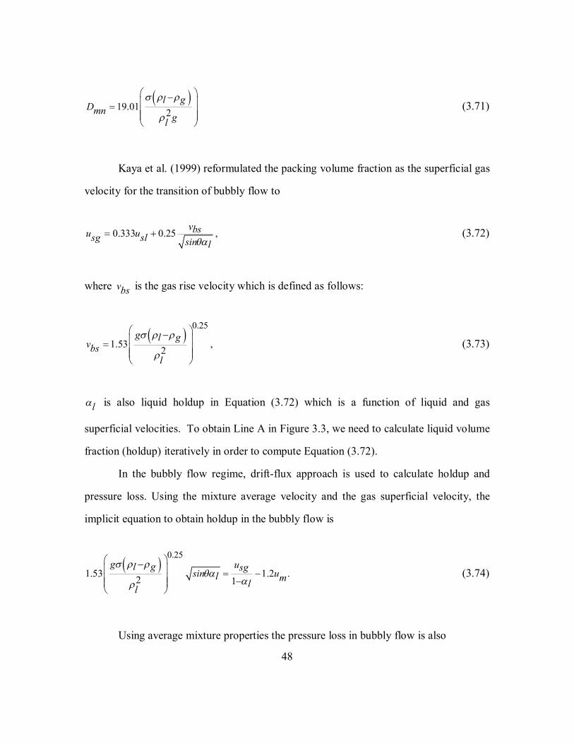
48
19.01 2
l gDmn
gl (3.71)
Kaya et al. (1999) reformulated the packing volume fraction as the superficial gas
velocity for the transition of bubbly flow to
0.333 0.25 ,
vbsu usg sl sin l
(3.72)
where vbs is the gas rise velocity which is defined as follows:
0.25
1.53 ,2
g l gvbs
l (3.73)
l is also liquid holdup in Equation (3.72) which is a function of liquid and gas
superficial velocities. To obtain Line A in Figure 3.3, we need to calculate liquid volume
fraction (holdup) iteratively in order to compute Equation (3.72).
In the bubbly flow regime, drift-flux approach is used to calculate holdup and
pressure loss. Using the mixture average velocity and the gas superficial velocity, the
implicit equation to obtain holdup in the bubbly flow is
0.25
1.53 1.2 .2 1
g ul g sgsin ul mll (3.74)
Using average mixture properties the pressure loss in bubbly flow is also

49
2
.2
f uP m m mgsinm Dl
(3.75)
Dispersed Bubbly Flow Transition. Dispersed bubbly flow can exist in high
flow rates, where a strong turbulent force can break large bubbles into small ones. This
mechanism is maintained until the volume fraction of gas is below a certain limit. Once
the gas volume fraction increases, the turbulent force cannot prevent bubble
agglomeration and cannot break the bubbles to small ones. At this condition a chaotic
slug flow is observed.
The maximum diameter of stable dispersed bubble (Barnea et al. (1982)) is
0.5 0.6 0.4
1.24.15 0.725 .2
u fsg mD umx mu u Dsg sl l (3.76)
Dispersed bubbly flow exists if the maximum stable bubble size is smaller than
the critical bubble size (Line B Figure 3.3).The critical bubble size proposed by Taitel et
al. (1980) is
0.50.42.0 .
DCD g l g (3.77)
Barnea modified the Tatiel model to DCB and considered the inclination effect for
critical bubble size,
50
23.0 .8.0
f ul m mDCB gsinl g (3.78)
The transition of dispersed bubbly flow to slug (Line C in Figure 3.3) is also
obtained from maximum gas volume fraction of 0.52. This criterion in terms of
superficial gas and liquid velocities becomes
1.083 .u usg sl (3.79)
In dispersed bubbly flow the holdup is calculated from no slip holdup
.
usll u usl sg
(3.80)
and similar to bubbly flow, Equation (3.75) is used for the total pressure loss.
Slug Flow Transition. Increasing the gas superficial velocity can change slug
flow to a more chaotic flow, churn or annular flow. Kaya et al. (1999) showed that the
transition of the slug to churn flow (Line D in Figure 3.3) can occur at
12.19 1.2 , u u vsg osg (3.81)
where vo is Taylor bubble rise velocity
0.5
0.35 0.54 .
gD l gv sin coso l
(3.82)

51
In the slug flow condition, since we have elongated bubbles and liquids (Figure
3.3), the method of holdup and pressure loss calculation is more complicated than that of
bubbly and dispersed bubbly flow. In this flow regime, we calculate holdup and pressure
loss by the following procedure. Assuming
0.25
1.53 ,2
g l gv
l (3.83)
0.5
1.25 0.35 ,
gD l gv uTB m l
(3.84)
the variables in the liquid slug unit are calculated as
,1.208 0.921
GLS
usgHu vm
(3.85)
1 , LLS GLSH H (3.86)
1.08 0.921 , mGLSv u v (3.87)
,
GLS
LLS
m GLSLLSv
u H vH
(3.88)
where, HGLS is the gas volume fraction, HLLS is the liquid volume fraction, vGLS is
gas velocity and vLLS is the liquid velocity in the liquid slug unit.
The variables in Taylor bubble also can be calculated iteratively as
0.59.916 1 , GTBLTBv gD H (3.89)
1 ,
TB LLS LLSGTB TB LTB
v v HH
v v (3.90)

52
1 . LTB GTBH H (3.91)
Using the liquid slug and the Taylor bubble variables, the ratio of Taylor bubble
length to slug unit is obtained
1 .
TB LLS LLS TB LTB
TB GTB GLS
u v v H v Hslv H H
(3.92)
In addition, the liquid slug density and viscosity are updated as follows:
, LLS GLSH Hls l g (3.93)
. LLS GLSH Hls l g (3.94)
Furhtermore, the liquid holdup and the pressure loss in fully developed slug flow
are calcualted as follows:
(1 ) , LLS LTBH Hl (3.95) 2
(1 ).2
f uP ls ls mgsinlsl D
(3.96)
For churn flow, pressure loss and holdup calculation, similar to the approach pursued for
slug flow, is applied.
Annular Flow Transition. In annular flow regime, a gas core is observed that is
surrounded by a thin liquid film. Taitel et al. (1980) showed that the annular flow regime occurs when the gas superficial velocity exceeds a critical value vgc

53
0.25
3.1 .2
g l gvgc
g (3.97)
In addition to critical gas velocity, Hasan et al. (2007) added a minimum gas
volume fraction of 0.7 to the criteria of existing annular flow. Line E in Figure 3.3
represents the Taitel et al. (1980) and the Hasan et al. (2007) annular flow transition
border.
Kaya et al. (1999), following the approach by Ansari et al. (1994), slightly
modified the annular flow transition criterion. In this approach, the annular flow is
changed to slug flow when the liquid film becomes unstable. From mathematical point of
view, this condition is satisfied when
2
32 1.5 ,
(1 1.5 )
HLFY XM MH HLFLF (3.98)
0.12.
ACHLF LC A (3.99)
LFH is the liquid film holdup, a function of dimensionless liquid film thickness
( ). MY and MX are modified Lockhart-Martinelli (1949) parameters which are
functions of liquid entrainment fraction in the gas core ( FE ) and superficial frictional
pressure gradients for liquid and gas core.
4 (1 ), HLF (3.100)
2
2.5 30,
4 1 1 4 1 4 1
XZ MYM (3.101)

54
,
gsin l cYM dP dL SC
(3.102)
21 , SL
SC
dP dLfFX FEM f dP dLSL (3.103)
1 0.125 1000 1.5 ,
usg g gFE expl
(3.104)
1 300 Z for 0.9,FE (3.105) 1/3
1
lZc
for 0.9,FE
.
FE usl
LC FE u usl sg (3.106)
In Equations (3.98) through (3.106), the gas core properties are calculated by
volumetric averaging of entrained liquid and gas properties. Details of the other related
parameters can be found in Kaya et al. (1999) and Ansari et al. (1994).
Finally, to compute the pressure loss and holdup in annular flow, we use the
following equations
,
ACHl LF LC A (3.107)
.51 2
SC
ZP dPgsincl dL (3.108)
The annular flow transition proposed by Ansari et al. (1994) and Kaya et al.
(1999) predicts the annular flow regime in higher gas superficial velocity than the Taitel
et al .(1980) and the Hasan et al. (2007) approaches. For this reason, to mitigate this
discrepancy in UTWELL, both options have been considered in the vertical annular flow
detection.

55
3.5.2 Flow Patterns in Horizontal Wells
For horizontal or near-horizontal wells, four flow patterns have generally been
introduced (Shoham, 2005). Although, these flow patterns can be sub-divided into
slightly different flow regimes, in order to avoid situations that are more complex we
only consider them as main flow configurations. Stratified, bubbly, intermittent, and
annular flows as shown in Figure 3.4 are the main flow regimes researchers have agreed
upon for the horizontal flow (Shoham, 2005).
For horizontal flow pattern detection, we follow a procedure similar to Shoham’s
(2005). The first step in flow pattern detection in horizontal inclinations is recognizing
the stratified flow regime. For this purpose, the Kelvin-Helmholtz constraint is verified to
check whether the stratified flow can exist or not. With this constraint, when the gas
actual velocity exceeds a critical velocity, the flow regime can no longer be stratified.
0.5
1 .
gcos Al g ghug D dA dhg l (3.109)
Assuming non-dimensional form of the variables in the expression (3.109), we obtain the
stratified flow transition when
0 ,F F (3.110)
where
0.52
1,2
h Al gFu Sg i
(3.111)

56
0.5
.0
gF usgDgcos l g
(3.112)
The key parameter in Equation (3.111) is lhhD
. All the other parameters (i.e. iS , gA )
can be calculated as a function of lh (Shoham (2005), page 67).
lh can be obtained from momentum equations of liquid and gas in stratified flow
condition. Assuming separate flows for gas and liquid and neglecting the axial holdup
gradient and momentum acceleration terms, we have
0,
S SP wg g i i gsingx A Ag g (3.113)
0.
S SP wl l i i gsinlx A Al l (3.114)
Subtracting (3.113) from (3.114) we obtain
1 1 ) 0.(
i iS Swg g wl l gsinl gA A A Ag l g l
S (3.115)
In Equation (3.115), Sl is the wetted perimeter by liquid phase, Sg is the wetted perimeter
by gas phase and Si is the interphase perimeter. Ag and Al are gas and liquid phase cross-
sectional areas. All the parameters in Equation (3.115) can be written as a function of
liquid level, velocities and fluid properties. In addition, Equation (3.115) can be
transformed to non-dimensional form as in

57
2
2 2 4 0,
u S Smn l S Sgl i iX u d u d u Yl l g g gA A A Al g g l
(3.116)
2 ,dP dl SLXdP dl SG
(3.117)
.
gsinl gY
dP dl SG (3.118)
Solution of the equation (3.116) yields lh . For flow regime detection, if the
calculated lh satisfies condition in (3.110), the system has non-stratified flow; otherwise,
the system has stratified flow. If system became non-stratified and the non-dimensional
liquid level turned out to be less than 0.35, system would be assumed to have bubbly
flow; otherwise, constraint (3.119) would be verified:
0 ,T T (3.119)
0.5
0.22
8,
g
l i l l
AT
u S u d (3.120)
0.5
0 .
SL
l g
dP dlT
gcos (3.121)
If constraint (3.119) is satisfied, the dominant flow regime is intermittent flow;
otherwise, it is annular flow.
Once we define the system’s dominant flow pattern, the holdup and the pressure
loss can be calculated accordingly. The pressure loss and the holdup for bubbly,
intermittent, and annular flow are calculated in a fashion similar to deviated wells’ except

58
with some corrections for the inclination angle. However, for the stratified flow, the
holdup and the pressure loss are computed as follows:
, l lDh (3.122)
.
wl l i i
l l
P gsinllS S
A A (3.123)
Closing the section on flow pattern detection, we also pay attention to few
convergence issues related to flow regime transitions. Since flow pattern transitions
introduce discontinuities in the two-fluid models, the transitions criteria should be
smoothened. In the UTWELL development for steady-state flow models, the flow
regimes are selected based on the same approaches given in Sections 3.5.1 and 3.5.2.
However, for transient models, since discontinuities can cause severe problems, the
transition criteria are slightly modified for using RELAP5 (2012) to avoid stability
problems.
3.6 CONSTITUTIVE RELATIONS
The constitutive models referred to in this section are the equations we apply for
correlations of phasic velocities in the drift-flux models and for interphase drag forces in
the two-fluid models. These relations are required in the momentum equations to grant a
closure to the system of equations.

59
3.6.1 Drift-flux Model
The slippage between two fluids results from the non-uniform profile of velocity
and buoyancy forces between the phases. This phenomenon can be modeled for a mixture
of gas and liquid by a mathematical equation (Shi et al., 2005) as follows:
0 , g gl m glu C u Vd (3.124)
01.
1 1
g gl gl m gl
g g
Cu u Vd (3.125)
0glC is a profile parameter, mu is volumetric average mixture velocity, and glVd is
drift velocity. Hasan and Kabir (1999) applied a similar model for the mixture of water
and oil as in
0 , o ow l owu C u Vd (3.126)
0 .
l o ow o
w l oww w
Cu u Vd (3.127)
Substituting liquid velocity lu from Equation (3.125) to Equations (3.126) and
(3.127), oil and water velocities can eventually become a function of mixture velocity as
well:
00 0
1,
1 1
g gl go ow m ow gl ow
g g
Cu C u C Vd Vd (3.128)

60
0 00
0
1 11 1
1
+ .1
g gl g gll o ow
g g glw m gl
w w g
go oow gl ow
w g w
C CC
u u Vd
C Vd Vd
(3.129)
The key parameters in the drift flux models are the profile parameters and the drift
velocities for liquid/gas and oil/water systems. These variables are dependent on the flow
regime condition and the spatial distribution of the fluids as well. Shi et al. (2005) and
Hasan and Kabir (2007) proposed general algorithms to define the drift-flux parameters.
They showed that by using some interpolation rules, the drift-flux parameters can also
become continuous in the entire range of solutions.
Figure 3.6 shows the drift flux parameters that we have calculated for a typical oil
( 58 , 1.0 , 103
lb dyne
Cpo o ow cmft), gas ( 0.077 , 0.018 , 36
3
lb dyneCpg g gl cmft
) and
water ( 63.4 , 1.03
lb
Cpw wft
) mixture in a pipe with 0.498 ft diameter from drift-flux
model in UTWELL. The trends of curves that we obtained are similar to Shi et al. (2005)
solutions for default drift-flux coefficients.
Furthermore, if the mixture velocity in the drift-flux model is obtained as mass
average velocity, the drift-flux equations should be modified accordingly. Using
Equations (3.130) and (3.131), the new drift-flux model for mass average mixture
velocity is obtained as follows:
0 , g gl g g l l glu C u u Vd (3.130)
, g g g l l l m mu u u (3.131)

61
10
1 ,
1 11 1 00
ll C glmmu u Vdg m gl
l gl g CC gl ggl gmm
(3.132)
101 .
1 11 1 00
g gg g C gll ml mu u Vdl m gl
l gl g CC gl ggl gmm
(3.133)
3.6.2 Two-fluid Model
The interphase velocity ( iu ) and the interphase friction force ( FI ) as shown in
Equations (3.25) and (3.26) are the two main parameters in the momentum equation
calculations that have been left undetermined so far. In this section, we introduce few
constitutive relations used for calculating these parameters.
First, the undetermined terms, iu , can be correlated to the velocities of gas and
liquid using a weighting factor as follows:
(1 ) , i g lu u u (3.134)
where, can be defined with a constant value (0.5) to yield the average velocities of liquid and gas or can be defined as 0 , when 0 g ; and 1 , when 0 g . In
UTWELL development, we used 0.5 for the entire solution.
The second undetermined term in momentum equations is the interphase shear
force coefficient ( FI ). This term is flow regime-dependent, which can be related to shear force per unit volume of gas and liquid phases ( igF and ilF ) in the momentum equations.

62
ig FIG u ug lg gF (3.135)
il FIL u ug ll lF (3.136)
Manipulation of Equations (3.135) and (3.136), in consideration of Equation
(3.26), can yield a new formulation for FI
.
ig il
g g l lu ug lm
F F
FI (3.137)
Assuming ig il iF F F , Equation (3.137) becomes a function of global
interphase friction force iF . Consequently, if we define a constitutive relation for iF , we
can define the constitutive relations for FI . Since FI is related to FIG and FIL via
Equation (3.26), defining a constitutive relation for FI can yield a constitutive relation
for FIG and FIL as well. iF is a flow-regime dependent parameter, which can be
obtained for two category of flow regimes: dispersed flow and separated flow. In
dispersed flows (such as bubbly, slug, churn, intermittent), the interphase friction force
per unit volume can be correlated as
,i i r rF C V V (3.138)
using drift velocity of the gas phase where,
00
1,
1
g glr g gl l
g
CV u C u (3.139)

63
3
2 .
g l l g
igl
gsinC
Vd (3.140)
In separated flows (such as stratified and annular), the interphase friction force
per unit volume can be correlated as
1 ,8 i c g l g l D F glF u u u u C S a (3.141)
using the drag force effect, where c is the continuous phase density, DC is drag
coefficient, FS is shape factor, and gla is interfacial area per unit volume.
Equations (3.138) and (3.141) can be computed for whole range of conditions
using appropriate drift-flux parameters from Section 3.6.1 and appropriate correlations
for drag force parameters from RELAP5 (2012). Figure 3.7 shows an example of FI
calculation for different liquid and gas velocities and gas volume fractions. In this
example, the flow regimes are only bubbly and slug. As can be seen, when the liquid and
gas velocity difference becomes larger, the drag force coefficient FI becomes larger as
well. In addition, when one of the phases disappears or its volume fraction decreases, the
interphase coefficient decreases too. The absolute value of interphase friction coefficient
can be an order of magnitude different for various flow conditions. The largest values are
usually obtained in bubbly flows, where the liquid and gas contact area is the largest.
3.7 PHASIC WALL FRICTION
In the momentum equations, there are wall friction terms ( FWL and FWG ) that
contribute the interaction of wall with the fluids. Defining a correct mathematical model

64
for these terms is crucial since they significantly contribute to pressure drop at high flow
rates. Wall friction terms are function of wall roughness, velocity of phases, and surface
contact of fluids with wall. To calculate wall friction terms, first we define a two-phase
wall friction term. Afterward, we split it to friction forces of liquid and gas phases by a
partitioning factor. Equation (3.142) shows the two-phase wall friction term, where lf is
the liquid phase friction factor, gf is the gas phase friction factor and C is the correlation
coefficient. These parameters have been discussed in (RELAP, 2012) with all details of
calculation.
0.52 22 21
22
dP f u C f u f u f ul l l l l l l l g g g g g g g gdl D (3.142)
The partitioning factor is calculated as
2
2
2,
lwf ul l l lZgwf ug g gg
(3.143)
where lw and lw are liquid and gas fractions on the wall. These fractions are defined
for each flow regime. Using Equations (3.142) and (3.143) FWL and FWG become
2
21 ,
2
dP ZFWLu dll l Zg l
(3.144)
21 1 .
2
dPFWGu dlg g Zg l
(3.145)

65
Figure 3.8 shows an example of results for the wall friction force coefficients,
FWG and FWL , as a function of liquid and gas velocities. As can be seen, for bubbly and
slug flows, the liquid wall friction is an order of magnitude larger than the gas wall
friction since gas does not contact with wall as much as liquid does.
3.8 INTERPHASE MASS TRANSFER
Interphase mass transfer g is another undetermined term in mass conservation
equations. This parameter defines the amount of gas that can evaporate or condensate
between hydrocarbon gas and liquid system. Figure 3.9 shows control volume of a liquid
and gas system that can exchange mass. Since the amount of gas that is exchanged
between the phases depends on pressure and temperature variations in the control volume, g is computed as a function of pressure and temperature. Equation (3.146)
illustrates the magnitude of gas mass transfer between oil and gas.
,
5.615
R RP Ps s uo o oP t P xgscg B R RT To s s uo o oT t T x
(3.146)
where Rs is solution gas oil ratio, Bo is oil formation volume factor, and gsc is gas
standard density. These parameters can be calculated using either blackoil correlations or
compositional models of hydrocarbon phases.
3.9 STATE RELATIONS
The primary variables that are calculated from the system of mass conservation
and momentum conservation equations in multiphase flow models are pressure, liquid

66
and gas volume fractions, and liquid and gas velocities. Other variables that appeared in
the equations are dependent variables and are calculated as functions of the primary
variables. Among the dependent variables, the ones that are related to fluid properties
(density, viscosity, interfacial tensions, solution gas oil ratio, and oil formation volume
factor) are state variables calculated from state relations.
In the development of UTWELL, there are two approaches to calculate state
relations. One approach is based on empirical correlations, called blackoil models. The
other approach is based on equation-of-state compositional models. These models have
been developed under the phase behavior modules, where all the properties of the fluids
(such as density, viscosity, enthalpy, compositions, and interfacial tensions) and the
derivatives of properties with respect to pressure and temperature are computed.
Appendices B and C show the details of property calculations in UTWELL. We
use Equation-of-State compositional approach and blackoil correlations, respectively.

67
Figure 3.1 Schematic view of stratified flow in horizontal wells.
(a) (b) (c) (d) (e)
Figure 3.2 Schematic views of flow regimes in vertical wells, (a) bubbly flow, (b) slug flow, (c) churn flow, (d) annular flow (e) disperse bubbly flow.
Gas
Liquid D/2
y
h
Pg
Pl
Pi

68
10-1
100
101
102
10-1
100
101
102
USG[ft/sec]
USL[
ft/se
c]
LINEALINEBLINECLINEDLINEE
Figure 3.3 Flow pattern map detection for vertical and deviated wells, reproduced from Kaya et al. (1999), Ansari et al. (1994) and Hasan and Kabir (2007).
(a) (b) (c) (d)
Figure 3.4 Schematic views of flow regimes in horizontal wells, (a) stratified flow, (b) bubbly flow, (c) intermittent flow, (d) annular flow.
Disperse Bubbly
Bubbly
Slug
Churn
Annular

69
0 0.2 0.4 0.6 0.8 110
-3
10-2
10-1
100
101
hL/d
F or
T
LINEALINEBLINEC
Figure 3.5 Flow pattern map for horizontal well, reproduced from Taitel and Dukler (1976) and Shoham (2005).
0 0.5 11
1.05
1.1
1.15
1.2
C0g
l
g
0 0.2 0.4 0.6 0.8 10
0.5
1
1.5
2
Vd gl
[ft/s
ec]
g
(a) (b)
Annular
Intermittent
Stratified
Bubbly

70
0 0.5 11
1.05
1.1
1.15
1.2C
0ow
o
0 0.2 0.4 0.6 0.8 10
0.1
0.2
0.3
0.4
Vd ow
[ft/s
ec]
o
(c) (d)
Figure 3.6 Drift-flux models (a) gas-liquid profile coefficient (C0gl), gas-liquid drift velocity (Vdgl), oil-water profile parameter (C0ow), oil-water drift velocity (Vdow).
0 2 4 6 8 100
1
2
3
4
5
Gas Velocity (ft/sec)
Liqu
id V
eloc
ity (f
t/sec
)
0.1
0.2
0.3
0.4
0.5
0.6
0.7
0.8
0.9
(a)

71
0 2 4 6 8 100
1
2
3
4
5
Gas Velocity (ft/sec)
Liqu
id V
eloc
ity (f
t/sec
)
0
5
10
15
20
25
(b)
Figure 3.7 An example of interphase friction force coefficient calculation for various liquid and gas velocities, (a) gas volume fraction (b) FI
0 2 4 6 8 100
1
2
3
4
5
Gas Velocity (ft/sec)
Liqu
id V
eloc
ity (f
t/sec
)
0.05
0.1
0.15
0.2
0.25
(a)

72
0 2 4 6 8 100
1
2
3
4
5
Gas Velocity (ft/sec)
Liqu
id V
eloc
ity (f
t/sec
)
500
1000
1500
2000
2500
(b)
Figure 3.8 An example of phasic wall friction calculation for various liquid and gas velocities, (a) FWG, (b) FWL.
Figure 3.9 Schematic view of liquid gas equilibrium and interphase mass transfers.
Free gas
Liquid with solution gas

73
Chapter 4: Wellbore Heat Transfer Models
Transportation of fluids in the wellbore always involves heat transfer between the
fluid and its surrounding during production or injection processes. Most of the time,
controlling the amount of heat exchange between these two systems is important in field
operations. For example, in hot fluid injection heat-loss management is one of the crucial
tasks to target the desired temperature of the injection process. In production systems,
also monitoring the temperature of the fluid is important to control the route the fluid
moves in its phase envelope. In fact, some hydrocarbon fluids can create precipitates and
flow assurance problems at certain temperatures.
In this chapter, we study the process of heat transfer between wellbore and the
surrounding (ambience), solving the coupled wellbore/surrounding energy equations.
With the energy equation for the ambient and the wellbore taken into account, more
accurate results are obtained for fluid temperature. In addition, since temperature affects
the fluids’ properties, a better approximation of temperature can yield a better
approximation of flow rates and pressure.
4.1 ENERGY EQUATION IN THE WELLBORE
Although in reality the flowing liquid and gas temperatures are not equal, for the
sake of simplicity we assume they are identical in our application. Accordingly, the
energy equation that we solve to obtain fluid temperature in wellbore is the total energy
conservation:

74
22 2
22
22 2
221 1 1
ugu uo whh hg g go o o w w wg Jg J g Jc cc c c ct t t
uguo A u hA u h A u hg g g go o o o w w wg Jg J c cc cA x A x A
2
2
uww g Jc cx
uu u gw ogsin gsin gsinw o g w w o o g gg J g J g Jc c c c c c
0.Qloss
A (4.1)
In the above equation, ho , hg , hw are oil, gas and water enthalpies per unit mass,
g Jc c are the unit conversion factors, o , g and w are the oil, gas and water enthalpy
influxes per unit well gridblock volume.
The enthalpy can be related to the pressure and temperature via the heat capacity
(
pBtuC
F lbm) and Joule Thomson coefficient, ( 2
F
Btu ft):
144( ) , dh C dT C dPj pj j pjJc
, ,j o g w (4.2)
Hence, for any specific pressure and temperature, the liquid and gas enthalpies
can be calculated with respect to a reference pressure and temperature. The enthalpy
calculation is explained in detail in Appendices B and C for compositional and blackoil
models.

75
4.2 WELLBORE HEAT LOSS MODEL
In Equation (4.1), Qloss is the heat exchange, per unit length, between the fluid
and the surrounding formation. This term is defined as
2 ( ), Q r U T Tloss to to f wb (4.3)
where Uto is the overall heat transfer coefficient, Tf is the fluid temperature, rto is the
tubing outer radius and Twb is the formation temperature at the vicinity of the wellbore.
Overall heat transfer coefficient is defined on the basis of composite layer
geometry around the wellbore (Figure 4.1) and the heat transfer coefficient of each layer.
Equation (4.4) shows the final expression for Uto as function of radius and heat transfer
coefficient of composite layers
ln( / ) ln( / ) ln( / )1
( )ln( / )
.
r r r r r r r r r r rto to to ti to ins to to to co ciU r h k k r h h kto ti to t ins ins c r cas
r r rto wb cokcem
(4.4)
In Equation (4.4), the conduction heat transfer coefficients are user input values and the
convection heat transfer coefficients are calculated using appropriate correlations
(PIPESIM user manual, 2011).
4.3 AMBIENT TEMPERATURE MODEL
Heat transfer between the wellbore and the surrounding formation (ambient)
causes temperature change not only in the wellbore fluid but also in the ambient
formation. In Equation (4.3) Twb is the temperature of the ambient fluid at the contact

76
point of composite layer of wellbore and formation. Depending on the magnitude of the
heat transfer between wellbore and ambience, Twb can be significantly different than
formation temperature far from wellbore. At a distance far from wellbore (~100ft), a
constant geothermal temperature gradient can be maintained from top to the bottom of
formation. However, getting closer to the wellbore this gradient is no longer constant.
Since ambient temperature is integrated with the heat loss calculation, an accurate
estimation of this variable is crucial. In this section, we introduce robust numerical and
analytical models for ambient temperature calculation that can be applied in the heat loss
equation. Our analytical model is similar to Ramey’s (1962) model with some
modifications to include the superposition effect. In fact, Ramey’s model is not
sufficiently correct for wellbore temperature calculation during wellbore shutdown and
startup conditions.
Assuming a cylindrical geometry around the wellbore, an axisymmetric two-
dimensional model can be considered for heat transfer into the formation domain (Figure
4.2). Considering Fourier heat conduction in two-dimensional cylindrical geometry, the
mathematical formulation of ambient temperature becomes
1 1 ,
TT Trr r z tr z e
(4.5)
where e is heat diffusivity coefficient
.
Cpe ee Ke (4.6)

77
To solve Equation (4.5) appropriate initial condition and boundary conditions
should be applied. Equation (4.7) shows the initial distribution of ambient temperature
and Equations (4.8) through (4.11) show the boundary conditions.
( , , 0) ,
T Tbh surfT r z T l zzbh lz (4.7)
,2
QT zr Kr wb erwb
(4.8)
0,
Tr r
(4.9)
( , 0, ) ,T r t Tsurf (4.10)
( , , ) .T r l t Tz bh (4.11)
One approach to obtain the ambient temperature from Equation (4.5) is
discretizing the equation with finite difference schemes and solving it numerically
(Erickson and Mai, 1992). Since in the discretization of Equation (4.5), logarithmic
distances are used in the radial direction, we substitute r with a new variable r ln r
in order to be able to discretize the equation linearly in the r-direction. Hence, we obtain
12 * .* *
TT Tre rz tz er r
(4.12)
The discretized form of Equation (4.12) yields a system of linear equations as
1 1 1 1 1 ,1, , 1, , 1 , 11, , 1, , 1 , 1 ,
n n n n n na T a T a T a T a T Ti k i k i k i k i ki k i k i k i k i k i k (4.13)
where

78
1, 1,2
2,
i k i k
trieeri
a a (4.14)
,2
21),2(2 2
i kt triee e
r zi ka (4.15)
, 1 , 1 .2
i k i kt
ezk
a a (4.16)
Using NR grids in the r-direction and NZ grids in the z-direction the gridblock
dimension sizes are obtained as
,
relnrwbr
NR (4.17)
. lzz
NZ (4.18)
The discretized form of the boundary conditions for Equation (4.13) is also
defined as
0 ( ) ,,
T Tbh surfnT T l z izi k bh lz (4.19)
,,1 nT Ti surf (4.20)
,, nT Ti n bhz (4.21)
,1, 2, 2
Qrn n zT Tk k r Kwb e
(4.22)
., 1, n nT Tn k n kr r
(4.23)

79
Combining Equations (4.13) through (4.16) with Equations (4.19) through (4.23),
we obtain a system of linear equation that can be solved using a linear solver.
Another approach to solve Equation (4.5) is using analytical solutions for radial
geometry. If we assume that at r , the ambient temperature is found from a constant
geothermal gradient, we can only solve the Fourier heat conduction equation in the r-
direction. With this assumption, we actually neglect the heat transfer in the z-direction.
This assumption is reasonable at near wellbore since the temperature gradient in the z-
direction is much smaller than the r-direction. Hence, Equation (4.5) can be simplified to
1 1 .
TTrr r tr e
(4.24)
Considering
,Drr
rwb (4.25)
2,
D
ttre wb
(4.26)
02 ,
DT TT Ke Qz
(4.27)
Equation (4.24) can be written in non-dimensional form as
1 .
DDD
D D DD
TTrr r tr
(4.28)
The initial condition and boundary conditions for Equation (4.28) are also defined
in non-dimensional form as in

80
( ,0) 0,D DT r (4.29)
1,1
DD
D D
Trr r
(4.30)
( , ) 0, D D DT r t (4.31)
0.
D
D
D r
Tr
(4.32)
The analytical solution for Equation (3.28) can be divided into three regions, the
early transient, later transient, and pseudo-steady state. When 0.12
ttDE re wbthe
solution is early transient as
2
( , ) 0.5 ,4
DD D D D
rT r t Ei t
(4.33)
when 0.1 tDE the solution is later transient as
214.6819
2 3( 1, ) 0.84 ,2 4
D D D
tDtD RT r t lnR e
R (4.34)
where reR
rwb. Finally, when DEt the solution is pseudo-steady state as
22 3( 1, ) .
4 D
D D DtT r t lnR
R (4.35)

81
Converting the non-dimensional temperature to actual temperature the final
solution for the ambient temperature becomes
( , )( , ) ( , ) ,0 2
I r tT r t T r t Qz Ke
(4.36)
where ( )I t is one of the solutions in early transient or later transient or pseudo-steady
state. Equations (4.36) is valid only if a constant heat exchange rate between well and the
formation is maintained. If the heat exchange rate becomes variable with time, the
solution for the ambient temperature is modified based on the superposition principle. In
variable heat flux condition, the ambient temperature solution becomes
1 ( , )( , )0( , ) ( , ) ( ) ( ) ( ) .0 0 12 21
t t tn I r t tI r t iT r t T r t Q t Q t Q tz z i z iK Ke et ti (4.37)
To evaluate the numerical and the analytical results, we made a comparison of
ambient temperature calculation for a cyclic hot fluid injection. Table 1 shows the
pertinent data for the well geometry. In this case, we injected hot fluid for three weeks
and then shut down the well. To avoid full simulation of the fluid temperature in the
wellbore, we assumed that the heat flux to the formation follows the curve shown in
Figure 4.3. With this example, we only want to test the solution results for ambient
temperature warm-up and cool-down processes.
Figure 4.4 shows the ambient temperature ( Twb ) at the vicinity of the wellbore at
a depth ( 2500Z ft ). As can be seen, the analytical solution with superposition (Equation
4.37) perfectly matches the numerical solution (Equation 4.13). However, the analytical
solution without superposition effect (Equation 4.36) over estimates the ambient
82
temperature during the warm-up period and underestimates the ambient temperature
during the cool-down period. Since in this case we had variable heat exchange between
wellbore and the formation, the analytical model without superposition is unable to
accurately predict the ambient temperature. However, at constant heat-loss between
wellbore and formation, the results for all methods are similar. Figure 4.5 illustrates same
results for both analytical and numerical calculation of the ambient temperature versus
time for a constant heat exchange of 20.
Btuhr ft
.
From the final results of numerical and analytical methods, we conclude that
analytical models inclusive of superposition effects can reasonably achieve the same
solution by numerical simulation. Since analytical methods are an order of magnitude
faster than numerical simulations, the application of those models is more desirable for
comprehensive wellbore modeling. Finally, since in reality the heat exchange between
wellbore and formation varies with time, the analytical models with superposition effect
is necessary for ambient temperature calculation.
.
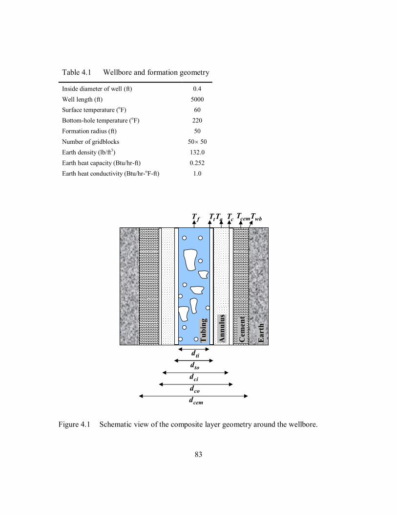
83
Figure 4.1 Schematic view of the composite layer geometry around the wellbore.
Table 4.1 Wellbore and formation geometry
Inside diameter of well (ft) 0.4 Well length (ft) 5000 Surface temperature (oF) 60 Bottom-hole temperature (oF) 220 Formation radius (ft) 50 Number of gridblocks 50 50 Earth density (lb/ft3) 132.0 Earth heat capacity (Btu/hr-ft) 0.252 Earth heat conductivity (Btu/hr-oF-ft) 1.0
Eart
h
Cem
ent
Ann
ulus
Tubi
ng
tid
tod
cod
cemd
fT tT aT cT cemT wbT
cid

84
Figure 4.2 Two-dimensional axisymmetric models for surrounding formation with initial temperature distribution.
0 200 400 600 800 10000
5
10
15
20
Time [hrs]
Hea
t Flu
x [B
tu /
hr.ft
]
Figure 4.3 Heat rate per unit length adsorption to the formation versus time.
Z
bhT
er
wbr
surfT

85
0 200 400 600 800 100088
90
92
94
96
98
100
102
Time [hrs]
Tem
pera
ture
[o F]
NumericalAnalytical1Analytical2
Figure 4.4 Comparison of numerical and analytical models (1 = with superposition, 2 = without superposition) results for ambient temperature calculation with variable heat exchange.
0 100 200 300 400 50088
90
92
94
96
98
100
102
Time [hrs]
Tem
pera
ture
[o F]
NumericalAnalytical1Analytical2
Figure 4.5 Comparison of numerical and analytical models (1= with superposition, 2 = without superposition) results for ambient temperature calculation with constant heat exchange.

86
Chapter 5: Wellbore Models Numerical Solutions
The UTWELL multiphase flow simulator solves six field equations to obtain six
primary variables defining the state of fluids in the wellbore. The primary variables
solved in UTWELL consist of volume fraction of water (w ), volume fraction of gas
(g ), pressure ( P ), velocity of gas ( ug ), velocity of liquid ( ul ) and temperature (T ).
These variables are used to update the secondary variables from state relations,
constitutive relations, and the phasic wall frictions.
In Chapters 3 and 4, we derived the basic differential equations that form
mathematical models of the field equations. We obtained one-dimensional multiphase
flow model along the well trajectory that includes mass conservation, momentum
conservation and energy conservation equations.
In this chapter, we introduce different numerical algorithms that can be used to
solve the field equations. We consider finite-difference methods to discretize the system
of equations. We also investigate various numerical methods, such as semi-implicit,
nearly implicit and fully implicit methods, to approximate the linearization of the
equations. Furthermore, in the following sections, we verify the solution results of
discretized equation for convergence, robustness, and accuracy against several test cases.
5.1 DISCRETIZATION OF FIELD EQUATIONS
One of the first steps in numerically solving a Partial Differential Equation (PDE)
is approximating the time and spatial derivatives and linearizing the equations. In this
section, we introduce the discretization of field equations with regard to flow models as
in two-fluid and drift-flux. Since two-fluid models are subjected to the ill-posedness

87
problem, employment of stabilizing techniques is necessary in the discretized equations.
However, since drift-flux models are always well-posed, they do not need extra care in
the discretization schemes.
Addition of second-order differential terms, such as viscous diffusivity terms, and
the virtual mass term in the phasic momentum equations proffers well-posedness to the
two-fluid model. Furthermore, selective implicit evaluation of spatial gradient terms at
the new time and donor based parameters for flux terms yields numerical stability of the
two-fluid models as well as faster computation time.
5.1.1 Discretization Method for Two-fluid Models
The guideline for discretization of the two-fluid model is listed as follows:
A staggered gridding is considered as shown in Figure 5.1. Junctions of the gridblocks
(vector nodes) are labeled with j index and the centers of gridblocks (scalar nodes) are
labeled with K, L, and M.
Pressure, temperature, and phase volume fractions are calculated in the center of the
gridblocks and the phase velocity vectors are calculated at the junction.
Liquid is the mixture of oil and water. The liquid phase properties are obtained from
volumetric or mass averaging. The velocity of oil and water can be attributed to the
velocity of liquid either using drift-flux approach or assuming no slip condition.
A selective implicit evaluation is used for spatial gradient terms. Implicit terms are
used only for velocities in mass and energy convection terms, pressure gradient in the
momentum equation and interface mass and momentum transfer in mass and
momentum equations.
A donor-like formulation is used for the flux terms.

88
Equations are reformulated in a way that can be degraded to single phase smoothly
when some phases are disappeared.
The final form of reformulated equations used in two-fluid model consists of
water mass conservation, liquid and gas mass conservation difference, liquid and gas
mass conservation summation, liquid and gas momentum conservation difference, liquid
and gas momentum conservation summation, and liquid and gas energy conservation
summation as
1 ,
A uw w w w wwt A x
(5.1)
1 2 ,
A u u ug g o o w w g g g o o o w w w
g g o wt A x (5.2)
1 ,
A u u ug g o o w w g g g o o o w w w
g o wt A x (5.3)
22
1 1144.02 2
( ) ( )
uu uu P yg gl l mg B u FWGc l g y gt t x x x xg lg l
u u u u ul l g g g l m i g g l lu FWL u u FIl g m g lg g l l g g l l
,
vm u ug lC mtg l
(5.4)
22
144.02 2
uu uu Pg gl l g Bcg g l l g g l l m xt t x x x
( ) , u FWG u FWL u u u ug g g l l l g g l g g l l (5.5)

89
2 2 2
2 2 2
ug u uo wh h hg g g o o o w w wg J g J g Jc c c c c ct t t
2 2 2
2 2 21 1 1
ug u uo wA u h A u h A u hg g g g o o o o w w w wg J g J g Jc c c c c cA x A x A x
u u ug o wgsin gsin gsinw o g g g o o w wg J g J g Jc c c c c c
.Qloss
A (5.6)
Equations (5.1) through (5.6) can be discretized to
Water Mass Conservation
1 1, , , , , ,
n n n n n nVb w L w L w L w L w L w L
1 1 ,,, , ,, 1 , 1 1 , 1 nn n n n n n n nt A u A u V tb w Lw j w j j w jw j w j j w j (5.7)
Gas and Liquid Mass Conservation Difference
1 1 1, , , , , , , , ,
n n n n n n n n nVb g L g L g L o L o L o L w L w L w L
1 1 1, , , , , , , , ,
n n n n n n n n nVb g L g L g L o L o L o L w L w L w L
1 1, , ,, 1 , 1 1 , 1
n n n n n n n nt A u A ug j g j j g jg j g j j g j
1 1, , ,, 1 , 1 1 , 1
n n n n n n n nt A u A uo j o j j o jo j o j j o j
1 1, , ,, 1 , 1 1 , 1
n n n n n n n nt A u A uw j w j j w jw j w j j w j
12 ,, , , n n n nV t gb g L o L w L (5.8)

90
Gas and Liquid Mass Conservation Summation
1 1 1, , , , , , , , ,
n n n n n n n n nVb g L g L g L o L o L o L w L w L w L
1 1 1, , , , , , , , ,
n n n n n n n n nVb g L g L g L o L o L o L w L w L w L
1 1, , ,, 1 , 1 1 , 1
n n n n n n n nt A u A ug j g j j g jg j g j j g j
1 1, , ,, 1 , 1 1 , 1
n n n n n n n nt A u A uo j o j j o jo j o j j o j
1 1, , ,, 1 , 1 1 , 1
n n n n n n n nt A u A uw j w j j w jw j w j j w j
,, , , n n nV tb g L o L w L (5.9)
Gas and Liquid Momentum Conservation Difference
2 1 11 , , , ,
nvmC n n n nmx u u u uj g j g j l j l jg l j
2 2 2 2( ) ( ) ( ) ( )2
n nt g g n n n nl lu u u ug gL K L Kl lg g l l jj
2
n nt g g n nl lVISG VISLj jg g l l jj
1 11 1144.0 , ,
nl g n n n nn nt g P P t x FWG u t x FWL uc j j g j j j l jL Kl g j
1 1 1( ) , , , , ,, , ,
g n n n n n n n n nt x u u uj j m j i j g j g j g jl j l j l jg g l l
1 1 1 1( ), , , n n n n n nt x f fwg u fwl uj x j j j g j j l jg g l l
1 1(1 ( 1)) (1 ( 1))1 0, , n n n n nt x FI f C u f C uj m x gl x glj g j jj l j
nn n nmt B y yl g y L Kjg l j

91
1 1, ,( ) ( ) .
n n
g g n n n nl lj j g j j l j
g g l l jj
g lg g l l
t x u u (5.10)
VISG and VISL in Equation (5.10) are the viscous-like terms for gas and liquid
phase that are added for the stability and well-posedness of the phasic momentum
equations. These terms are defined as
1 1 1 ,, ,, ,, 1 , 12
A Aj jn n n n n n nVISG u u u u u uj g j g jg L g Kg j g jA Aj j (5.11)
1 1 1 ., , 1 , , , , 12
A Aj jn n n n n n nVISL u u u u u uj l L l j l j l K l j l jA Aj j (5.12)
xf in Equation (5.10) is also the coefficient with the value of zero or one that
incorporates the extra terms for the dispersed drag model. When the flow regime is bubbly, slug or churn, xf is one; otherwise, it is zero. In dispersed flow, wgf and wlf are
added using the following equations to incorporate the surface drag forces of dispersed
phase and continuous phase.
, wl l g lf FWL (5.13)
. wg l g gf FWG (5.14)
The liquid and gas profile parameters 0glC and 1glC also appear in the dispersed
flow regimes, where 0glC is obtained from Chapter 3 and 1glC is defined as follows:
1 0 .1 1
Cg glC glg
(5.15)

92
Moreover, in the momentum difference equation for stratified flows, the gravity
term for liquid height gradient in the axial direction is incorporated as
nn n nmt B y yl g y L Kjg l j
where
1 ,2
Dy cosL (5.16)
, D cos sing (5.17)
.B gsiny (5.18)
Gas and Liquid Momentum Conservation Summation
1 1, , , ,
n nn n n nx u u u ug g l lj g j g j j l j l jj
2 2 2 2( ) ( ) ( ) ( )2
nt nn n n nu u u ug g g g l lL K L Kj l lj
2
nt nn nVISG VISLg g l lj jjj
1 1 1,144.0 ( ) ( ) n n n n n n
L K j m j x j g g j j g jgct P P t x B t x FWG u
11,( ) ( )
nn n n n
j l l j j l j j g j g l jt x FWL u t x u u
1 1, ,( ) ( ) . n n n n
j j g j j j l jg lt x u t x u (5.19)
Gas and Liquid Energy Conservation Summation 2 21( ) ( )1 1 1
, , , , , ,2 2
n nu uo on n n n n nL LV h hb o L o L o L o L o L o Lg J g Jc c c c
2 21( ) ( )1 1 1, , , , , ,2 2
n nu ug gn n n n n nL LV h hb g L g L g L g L g L g Lg J g Jc c c c
2 21( ) ( )1 1 1, , , , , ,2 2
n nu uw wn n n n n nL LV h hb w L w L w L w L w L w Lg J g Jc c c c

93
2 1 2 1( ) ( )11 1 1 1 1 1 1 1, , , ,1 , 1 , 1 , 1 , 1 2 2
n nu uo oj jn n n n n n n n n nt A u h A u hj o j o j o j o jj o j o j o j o j g J g Jc c c c
2 1 2 1( ) ( )11 1 1 1 1 1 1 1, , , ,1 , 1 , 1 , 1 , 1 2 2
n nu ug gj jn n n n n n n n n nt A u h A u hj g j g j g j g jj g j g j g j g j g J g Jc c c c
2 1 2 1( ) ( )11 1 1 1 1 1 1 1, , , ,1 , 1 , 1 , 1 , 1 2 2
n nu uw wj jn n n n n n n n n nt A u h A u hj w j w j w j w jj w j w j w j w j g J g Jc c c c
1 1 1, , ,
n n nV tb o L g L w L
11 1,, ,1 1 1 1 1 1
, , , , , ,
nn nuu ug Lo L w Ln n n n n nV t gsin gsin gsinb o L o L g L g L w L w Lg J g J g Jc c c c c c
, .
nQloss LV tb nAj (5.20)
In discretized equations, bV is the bulk volume of the gridblock, jx is the grid
size length, t is the time step size, n is time index, L is the gridblock center index, j is
gridblock junction index. In addition, parameters with dot (.) over-score correspond to
donor-like parameters or influx rate terms; parameters with tilde ( ~ ) are provisional
advanced time variables with intermediate value before the final update.
Since the primary variables in our linearized equations are only 1 n
w , 1 ng , 1n
lu , 1nug , 1nT , 1nP ; the secondary variables that appeared in
advanced time ( 1n ) are written as a function of primary variables. Hence, the following
auxiliary equations are combined with discretized equations to solve the system of
equations:
1 1 1, n n n
w o l (5.21)
94
1 1 1 1, n n nw o g (5.22)
1 1 ,0 n nu C u Vdo ow l ow (5.23)
1 1 ,0 n nu C u Vdw ow l ow (5.24)
1 1
,1 ,, ,5.615 ,
, ,
n nR Rn n n ns sP P T TL L L LP TL Ln n nn P Pgsc Ro Ln n ns K L ug o L o Ln P x jB Lo L
n nn T TR n ns K L uo L o LT x jL
(5.25)
1 1 1 ,, ,
n nn n n n n nw wP P T Tw L w L L L L LP TL L
(5.26)
1 1 1 ,, ,
n nn n n n n no oP P T To L o L L L L LP TL L
(5.27)
1 1 1 ., ,
n n
g gn n n n n nP P T Tg L g L L L L LP TL L (5.28)
Furthermore, the junction parameters (parameters defined at the junction without
the over-score dot) are calculated from the linear interpolation of neighboring cells and
donor-like parameters ( ) are defined as follows:
if 0u j ,
1 1 ,2 2
u j
K L K Lj u j (5.29)
if 0u j and ,P PK L
, j K (5.30)
if 0u j and ,P PK L

95
, j L (5.31)
if 0u j and ,P PK L
,
K K L Lj K L
(5.32)
where u j is the junction velocity for specific phase, K and L are the mass control
volume indices in the neighboring of junction and is the donor parameter (i.e. density).
5.1.2 Discretization Method for Drift-flux Model
Similar to two-fluid model, a staggered gridding is used for discretization of drift-
flux model. The mixture velocity vector is calculated at the junction and the pressure,
temperature, and phasic volume fractions are calculated in the center of the gridblock.
The discretized equations in the drift-flux model consist of water mass
conservation, liquid mass conservation, mixture mass conservation, mixture momentum
conservation and mixture energy conservation. The final forms of those equations are
1 ,
A uw w w w wwt A x
(5.33)
1 ,
A u uo o w w o o o w w wg o wt A x
(5.34)
1 ,
A u u ug g o o w w g g g o o o w w w
g o wt A x (5.35)
2 2 2
144.0 ,
u u ug g g o o o w w wu DPm m mg gsinc mt x x A (5.36)

96
2 2 2
2 2 2
ug u uo wh h hg g g o o o w w wg J g J g Jc c c c c ct t t
2 2 2
2 2 21 1 1
ug u uo wA u h A u h A u hg g g g o o o o w w w wg J g J g Jc c c c c cA x A x A x
.
u u u Qg o w lossgsin gsin gsinw o g g g o o w wg J g J g J Ac c c c c c (5.37)
Using a first-order upwind scheme, the discretized form of Equations (5.33)
through (5.37) becomes
Water Mass Conservation 1 1
, , , , n n n nVb w L w L w L w L
11 1 1 1 1 1 .,, , , , 1 , 1 1 , 1 nn n n n n n n nt A u A u V tb w Lw j w j j w j w j w j j w j (5.38)
Liquid Mass Conservation
1 1 1 1, , , , , , , ,
n n n n n n n nVb o L o L o L o L w L w L w L w L
1 1 1 1 1 1, , , , 1 , 1 1 , 1
n n n n n n n nt A u A uo j o j j o j o j o j j o j
1 1 1 1 1 1, , , , 1 , 1 1 , 1
n n n n n n n nt A u A uw j w j j w j w j w j j w j
1 1 1 ., , n n nV t gb o L w L (5.39)
Mixture Mass Conservation
1 1 1 1 1 1, , , , , , , , , , , ,
n n n n n n n n n n n nVb g L g L g L g L o L o L o L o L w L w L w L w L
1 1 1 1 1 1, , , , 1 , 1 1 , 1
n n n n n n n nt A u A ug j g j j g j g j g j j g j

97
1 1 1 1 1 1, , , , 1 , 1 1 , 1
n n n n n n n nt A u A uo j o j j o j o j o j j o j
1 1 1 1 1 1, , , , 1 , 1 1 , 1
n n n n n n n nt A u A uw j w j j w j w j w j j w j
., , , n n nV tb g L o L w L (5.40)
Mixture Momentum Conservation 1 1
, , , , n n n nx u uj m j m j m j m j
1 2 1 1 2 1( ) ( ), , n n n nu um mm L L m L Lt
1 1 1 1, ,144.0 . n n n n
L K j m j j m j nj
gcDt P P t x gsin t x
A (5.41)
Mixture Energy Conservation 2 21( ) ( )1 1 1
, , , , , ,2 2
n nu ug gn n n n n nL LV h hb g L g L g L g L g L g Lg J g Jc c c c
2 21( ) ( )1 1 1, , , , , ,2 2
n nu uo on n n n n nL LV h hb o L o L o L o L o L o Lg J g Jc c c c
2 21( ) ( )1 1 1, , , , , ,2 2
n nu uw wn n n n n nL LV h hb w L w L w L w L w L w Lg J g Jc c c c
2 12 1 ( )( ) 11 1 1 1 1 1 1 1 1 1,, , , , , , ,12 2
nn uu gg j jn n n n n n n n n nt A u h A u hj g jg L g L g L g K g K g K g Kjg J g Jc c c c
2 12 1 ( )( ) 11 1 1 1 1 1 1 1 1 1,, , , , , ,1 , 12 2
nn uu oo j jn n n n n n n n n nt A u h A u hj o jo L o L o L o K o K o Kj o jg J g Jc c c c
2 12 1 ( )( ) 11 1 1 1 1 1 1 1 1 1,, , , , , ,1 , 12 2
nn uu ww j jn n n n n n n n n nt A u h A u hj w jw L w L w L w K w K w Kj w jg J g Jc c c c
1 1 1, , ,
n n nV tb o L g L w L

98
1 1 1, , ,1 1 1 1 1 1
, , , , , ,
n n nu u ug L o L w Ln n n n n nV t gsin gsin gsinb g L g L o L o L w L w Lg J g J g Jc c c c c c
1, .
nQloss LV tb nAj (5.42)
5.2 WELLBORE BOUNDARY CONDITIONS
In UTWELL, we can assign different types of boundary conditions for the
wellbore. Figure 5.2 shows the arrangement of typical boundary conditions that can be
used for the transient multiphase flow in the wellbores or pipelines. As can be seen the
boundary nodes can be defined as
1) Pressure Node
2) Mass Flow Node
3) Mass Source Node
4) Closed Node
All of these boundary conditions are assigned to the junction of nodes at the inlet
or outlet except Mass Flow Node. For the inlet node, temperature, gas oil ratio, and water
cut; or the mass flow rate of gas, oil, and water are also defined.
To effectively implement the boundary conditions in our numerical calculation, we consider imaginary nodes with zero volume ( 0 x j ) at inlet and outlet and assign
the given boundary values to these nodes. In Section 5.3, the boundary node equations
are discussed in detail.
In addition to the boundary conditions defined in Figure 5.2, for the single-phase
flow and steady state multiphase flow, additional types of boundary conditions have been

99
considered in UTWELL. These boundary conditions are used for coupled
wellbore/reservoir models where we have
1) Constant Wellhead Flow Rate
2) Constant Bottom-hole Pressure
For Constant Wellhead Flow Rate, the well is operated at a pressure condition that
can honor the flow rate of liquid or oil, which is required at the wellhead. For Constant
Bottom-hole Pressure, the wellbore pressure in the zone connecting with the reservoir is
maintained constant at the given value and all the flow rates are calculated.
5.3 SOLUTION METHODS
The discretized equations in Section 5.1 are linearized into a system of equations
to solve for the primary variables. In this section, we introduce different algorithms to
construct the linear system of equations for various flow models (i.e. homogenous, drift
flux, two-fluid). First, we present semi-implicit and nearly-implicit algorithms to solve
the two-fluid models. These methods are armed with some numerical techniques to
decrease the computation time for such sophisticated models. Secondly, we discuss a
fully-implicit algorithm to linearize the discretized equations for the drift-flux model.
Since we obtained a non-linear system of equations in the discretized form of drift-flux
model, we use the Newton method for the linearization of the equations. The
simplification of two-fluid and drift flux models, with consideration of no slip condition,
also yields homogenous model.
Finally, we discuss the solution methods for steady-state multiphase flow models.
We use a marching algorithm to solve steady-state model.

100
5.3.1 Semi-Implicit Approach
Many multiphase flow simulators (such as OLGA, RELAP5, and CATHARE) use
semi-implicit methods to solve the field equations. These methods have shown a lot of
promise in regards to stability and robustness of multiphase flow model solutions. In the
UTWELL development, we chose this method to solve the transport equations in the two-fluid model. Hence, we used the semi-implicit approach to obtain 1 n
w , 1 ng , 1n
lu , 1nug , and 1nP from mass and momentum conservation equations. We decouple the
energy equation from the former equations and solve it separately to obtain temperature, 1nT .
Using the method explained in Section 5.2.1, the discretized equations are already
obtained as a linear function of primary variables. The discretized equations are partially
as function of advanced time and partially old time. The implicit variables are selected in
a way that gives better numerical stability. Once we generated the semi-implicit
discretized equations, we follow the following procedure to decouple the variables and
construct final shape of algebraic equations.
First, we setup the water mass conservation, difference of gas and liquid mass
conservation, and summation of liquid and gas mass conservation as functions of liquid
and gas velocities.
1 1 1( ,1) - ( , 2) - ( ,3) -, , , , n n n n n nA I A I A I P Pw L w L g L g L L L
1 1 1 11 1 0 1 1 0( ) ( )( ) ( )( ) ( )( ) ( )( ) .
n n n ng j g j l j l jB I G I u G I u L I u L I u (5.43)
1I corresponds to water mass conservation equation, 2I corresponds to difference
between gas and liquid mass conservation equation and 3I corresponds to summation

101
of gas and liquid mass conservation equation. Matrix A and vectors B, G and L are
obtained from Equations (5.7), (5.8) and (5.9). Decoupling Equation (5.43) for primary variable 1-n nP PL L can be obtained as
1 11 1 0
1 11 1 0
1 1 11-
1 1
(3) (3)( ) (3)( )
(3)( ) (3)( ) .
n ng j g j
n nl j l j
n nP P A A AL L
A A
B G u G u
L u L u (5.44)
We also setup the difference gas and liquid momentum equation and summation
of liquid and gas momentum equation to obtain liquid and gas velocities as a function of
pressure.
1 1 1 1( ,1)( ) ( , 2)( ) ( ) ( ) , n n n ng j l j L KX I u X I u Y I Z I P P (5.45)
1I corresponds to the difference of gas and liquid momentum equations and 2I
corresponds to summation of liquid and gas momentum equations. Matrix X and vectors
Y and Z are obtained from rearranging Equations (5.10) and (5.19). Solutions of Equation
(5.45) for liquid and gas velocities are
1 1 1 1 1( ) (1) (1) , n n ng j L Ku X Y X Z P P (5.46)
1 1 1 1 1( ) (2) (2) . n n nl j L Ku X Y X Z P P (5.47)
If we plug the velocity of gas and liquid in Equation (5.44), we obtain the final
formula for the pressure equation as follows:
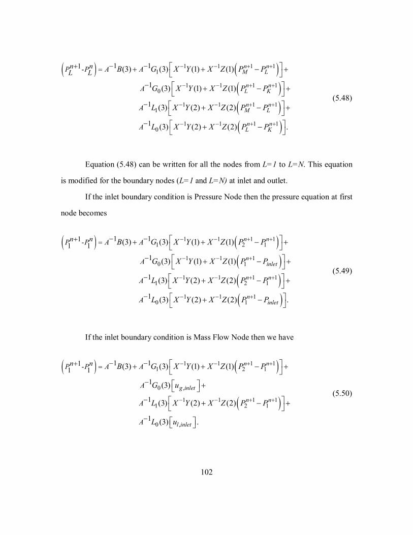
102
1 1 1 11
1 1 1 10
1 11
1 11-
1
1
(3) (3) (1) (1)
(3) (1) (1)
(3) (2) (2)
n nM L
n nL K
n nP P A AL L
A
A
B G X Y X Z P P
G X Y X Z P P
L X Y X Z
1 1
1 1 1 10
1 (3) (2) (2) .
n nM L
n nL KA
P P
L X Y X Z P P
(5.48)
Equation (5.48) can be written for all the nodes from L=1 to L=N. This equation
is modified for the boundary nodes (L=1 and L=N) at inlet and outlet.
If the inlet boundary condition is Pressure Node then the pressure equation at first
node becomes
1 1 1 11 2 1
1 1 10 1
1 11
1 11-1 1
1
1
(3) (3) (1) (1)
(3) (1) (1)
(3) (2) (2
n n
ninlet
n nP P A A
A
A
B G X Y X Z P P
G X Y X Z P P
L X Y X Z
1 12 1
1 1 10 1
1
)
(3) (2) (2) .
n n
ninletA
P P
L X Y X Z P P
(5.49)
If the inlet boundary condition is Mass Flow Node then we have
1 1 1 11 2 1
0 ,
1 1 1 11 2 1
1 11-1 11
1
(3) (3) (1) (1)
(3)
(3) (2) (2)
n n
g inlet
n n
n nP P A A
A
A
B G X Y X Z P P
G u
L X Y X Z P P
0 ,1 (3) . l inletA L u
(5.50)

103
Similarly, Equation (5.48) is modified for the outlet boundary condition at node
L=N. For Closed Node boundary condition, we use Mass Flow Node with zero value.
Considering Equation (5.48) with boundary node effects, a linear system of equations as
function of pressure is obtained. This equation can be solved by a tri-diagonal solver to
obtain pressure.
Next step in semi-implicit algorithm is updating the other primary variables after
calculating the pressure equation. Once we obtain the pressure, we can use Equations
(5.46) and (5.47) to calculate the velocity of gas and liquid, respectively. Afterward, we update the provisional advanced time water and gas volume fractions ( 1
, nw L and 1, ng L )
using Equation (5.43). Other provisional advanced time variables can be updated
accordingly.
Finally, we update the actual phasic volume fractions and the mixture density
using the unexpanded version of mass conservation of each phase as follows:
1( ) n
w w L 1 1 ,, , ,, , ,, 1 , 1 1 , 1
tn n nn n n n n n n nA u A u tw L w L w Lw j w j j w jw j w j j w jVb
(5.51)
1( ) no o L
1 1 1 1 ,, , , , , ,, 1 , 1 1 , 1
tn n n n n n n n n n n nA u A u t go L o L o j o j j o j o Lo j o j j o jVb (5.52)
1( ) ng g L
1 1 1 1 ,, , , , , ,, 1 , 1 1 , 1
tn n n n n n n n n n n nA u A u t gg L g L g j g j j g j g Lg j g j j g jVb (5.53)
11
1,
( )( ) ,
nn w w L
w L nw L
(5.54)
11
1,
( )( ) ,
nn o o L
o L no L
(5.55)
1 1 1( ) 1 ( ) ( ) . n n ng L o L w L (5.56)
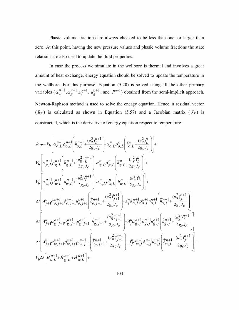
104
Phasic volume fractions are always checked to be less than one, or larger than
zero. At this point, having the new pressure values and phasic volume fractions the state
relations are also used to update the fluid properties.
In case the process we simulate in the wellbore is thermal and involves a great
amount of heat exchange, energy equation should be solved to update the temperature in
the wellbore. For this purpose, Equation (5.20) is solved using all the other primary variables ( 1 n
w , 1 ng , 1n
lu , 1nug , and 1nP ) obtained from the semi-implicit approach.
Newton-Raphson method is used to solve the energy equation. Hence, a residual vector
( TR ) is calculated as shown in Equation (5.57) and a Jacobian matrix ( TJ ) is
constructed, which is the derivative of energy equation respect to temperature.
2 21( ) ( )1 1 1
, , , , , ,2 2
n nu uo on n n n n nL LR V h hT b o L o L o L o L o L o Lg J g Jc c c c
2 21( ) ( )1 1 1, , , , , ,2 2
n nu ug gn n n n n nL LV h hb g L g L g L g L g L g Lg J g Jc c c c
2 21( ) ( )1 1 1, , , , , ,2 2
n nu uw wn n n n n nL LV h hb w L w L w L w L w L w Lg J g Jc c c c
2 1 2 1( ) ( )11 1 1 1 1 1 1 1, , , ,1 , 1 , 1 , 1 , 1 2 2
n nu uo oj jn n n n n n n n n nt A u h A u hj o j o j o j o jj o j o j o j o j g J g Jc c c c
2 1 2 1( ) ( )11 1 1 1 1 1 1 1, , , ,1 , 1 , 1 , 1 , 1 2 2
n nu ug gj jn n n n n n n n n nt A u h A u hj g j g j g j g jj g j g j g j g j g J g Jc c c c
2 1 2 1( ) ( )11 1 1 1 1 1 1 1, , , ,1 , 1 , 1 , 1 , 1 2 2
n nu uw wj jn n n n n n n n n nt A u h A u hj w j w j w j w jj w j w j w j w j g J g Jc c c c
1 1 1, , ,
n n nV tb o L g L w L
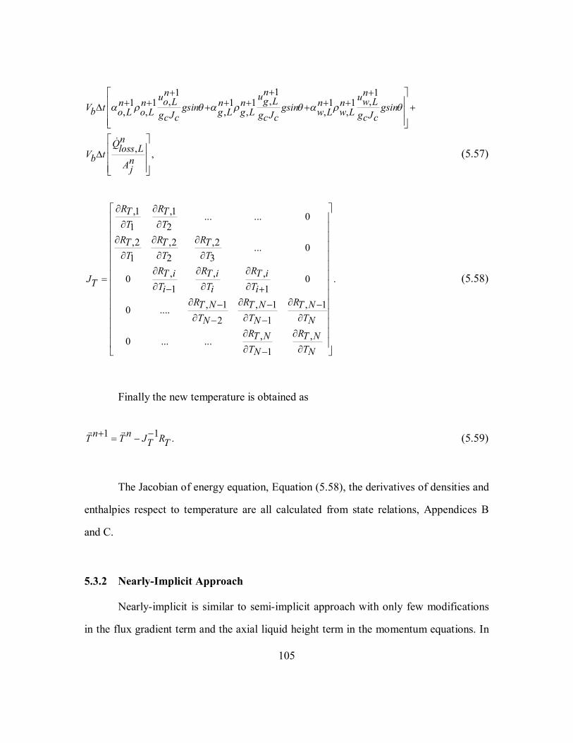
105
11 1,, ,1 1 1 1 1 1
, , , , , ,
nn nuu ug Lo L w Ln n n n n nV t gsin gsin gsinb o L o L g L g L w L w Lg J g J g Jc c c c c c
, ,
nQloss LV tb nAj (5.57)
,1 ,1 ... ... 0
1 2,2 ,2 ,2 ... 01 2 3
, , , .0 01 1
, 1 , 1 , 10 ....2 1
, ,0 ... ...1
R RT TT T
R R RT T TT T T
R R RT i T i T iJT T T Ti i iR R RT N T N T NT T TN N N
R RT N T NT TN N
(5.58)
Finally the new temperature is obtained as
1 1 .
n nT T J RT T (5.59)
The Jacobian of energy equation, Equation (5.58), the derivatives of densities and
enthalpies respect to temperature are all calculated from state relations, Appendices B
and C.
5.3.2 Nearly-Implicit Approach
Nearly-implicit is similar to semi-implicit approach with only few modifications
in the flux gradient term and the axial liquid height term in the momentum equations. In

106
semi-implicit approach, the momentum flux gradient was considered in an explicit
format. However, in the nearly-implicit method, this term is linearized into both implicit
and explicit terms. Recalling from Equations (5.10) and (5.19), the flux term derivatives
were calculated as
2 2 2 2( ) ( ) ( ) ( ) ,1 2
n nt g g n n n nl lu u u ug gL K L Kl lg g l l jj
2 2 2 2( ) ( ) ( ) ( ) .2 2
nt nn n n nu u u ug g g g l lL K L Kj l lj
In nearly-implicit method, those terms are replaced with the following equations
for momentum difference and momentum summation equations, respectively.
2 21
2 2
1 12( ) ( ) ( ) 2( ) ( ) ( ) ( ) ( )2
1 1 2( ) ( ) ( ) 2( ) ( ) ( ) ( ) ( )2
ng g
g g jn
l l
l l j
t n n n n n n n nu u u u u u u ug g g g g g g gL L L K K K L K
t n n n n n n n nu u u u u u u uL L L K K K L Kl l l l l l l l
2 22
2 2
1 12( ) ( ) ( ) 2( ) ( ) ( ) ( ) ( )2
1 1 2( ) ( ) ( ) 2( ) ( ) ( ) ( ) ( )2
ng g j
nl l j
t n n n n n n n nu u u u u u u ug g g g g g g gL L L K K K L K
t n n n n n n n nu u u u u u u uL L L K K K L Kl l l l l l l l
In addition, the axial liquid height gradient term
nn n nmt B y yl g y L Kjg l j
in
Equation (5.10) is converted to the implicit term as
nnmt Bl g yjg l j
1 1 n ny yL K . Consequently, this term is changed to a function of gas volume fraction

107
1 1 ., ,
n nn y n nmt Bl g y g L g Kjg l gj j
Considering the changes made in the momentum equations, the pressure equation
is not obtained as straightforwardly as in the semi-implicit method. Instead, in nearly-
implicit approach, the velocity equation is constructed first.
From Equation (5.43), we can obtain pressure and gas volume fractions as
functions of liquid and gas velocities as given below
1 1 1 1 11- (3) (3)( ) (3)( )1 1 01 1 1 1 (3)( ) (3)( ) ,1 1 0
n nn nP P A B A G u A G ug j g jL Ln nA L u A L ul j l j
(5.60)
1 1 1 1 11- (2) (2)( ) (2)( )1 1 0, ,1 1 1 1 (2)( ) (2)( ) .1 1 0
n nn n A B A G u A G ug j g jg L g Ln nA L u A L ul j l j
(5.61)
From momentum equations, after substitution of implicit terms, we also have
1 1 1(1,1)( ) (1, 2)( ) (1,3)( )1 11 1 1(1,4)( ) (1,5)( ) (1,6)( )1 1
1 1 1 1(1) (1) (1) ,, ,
n n nX u X u X ug j g j g jn n nX u X u X ul l ljj j
n n n nY Z P P VL K g L g K
(5.62)

108
1 1 1(2,1)( ) (2, 2)( ) (2, 3)( )1 11 1 1(2,4)( ) (2,5)( ) (2,6)( )1 1
1 1 1 1(2) (2) (2) ., ,
n n nX u X u X ug j g j g jn n nX u X u X ul l ljj j
n n n nY Z P P VL K g L g K
(5.63)
Substituting 1nPL and 1
, ng L from Equations (5.60) and (5.61) into Equations
(5.62) and (5.63), the system of equations is decoupled and becomes only functions of
liquid and gas velocities at advanced time. In this fashion, the velocities of liquid and gas
can be found from the final rearrangements in Equations (5.62) and (5.63). After solving
the velocities, pressure is updated from Equation (5.60) and the provisional gas and water
volume fractions are updated from Equation (5.43). Continuing the same approach, as
done for the semi-implicit method, we can also calculate the final values of primary
variables, using unexpanded phasic mass conservation equations.
Although in the nearly-implicit method we only made a small change in the
momentum equations, it caused much more complications in the calculation of primary
variables. Our experience shows that this small change also adds significant stability to
the two-fluid model, especially for the phase redistribution problems.
5.3.3 Fully-Implicit Approach
Fully implicit approach has been used to solve the drift-flux flow model in
UTWELL. Since the discretized equations for drift flux model are still non-linear with
fully implicit approach, we used Newton method to linearize the equations and solve for
primary variables. We decouple the energy equation from the mass and momentum
conservation equations similar to the semi-implicit and nearly-implicit methods. Hence,

109
we first solve the transport equation and then update the temperature, if thermal modeling
was involved.
In the Newton method, we solved the mass balance and momentum balance
equations by constructing a Jacobian matrix, J , and a residual vector, R , with primary
variables: mixture average velocity, pressure, liquid volume fraction, and water volume
fraction. As explained in Section 5.1.2, the equations we solve are 1f as mixture
momentum balance; 2f as mixture mass balance; 3f as liquid mass balance; 4f as water
mass balance.
1,1 1,1 1,1 1,1 1,1 1,1 1,1 1,1...
,1 1 ,1 ,1 , , ,
2,1 2,1 2,1 2,1 2,1 2,1 2,1 2,1...,1 1 ,1 ,1 , , ,
3,1 3,1 3,1 3,1 ..,1 1 ,1 ,1
f f f f f f f fu P u Pm l w m N N l N w Nf f f f f f f fu P u Pm l w m N N l N w Nf f f fu Pm l w
J
3,1 3,1 3,1 3,1., , ,
4,1 4,1 4,1 4,1 4,1 4,1 4,1 4,1...,1 1 ,1 ,1 , , ,
... ... ... ... ... ... ... ... ...
1, 1, 1, 1, 1, 1,...,1 1 ,1 ,1 ,
f f f fu Pm N N l N w N
f f f f f f f fu P u Pm l w m N N l N w N
f f f f f fN N N N Nu P um l w m N
1, 1,1, ,
2, 2, 2, 2, 2, 2, 2, 2,1...,1 1 ,1 ,1 , , ,
3, 3, 3, 3, 3, 3, 3, 3,1...,1 1 ,1 ,1 , , ,
4, 4,,1 1
f fN NPN l N w N
f f f f f f f fN N N N N N Nu P u Pm l w m N N l N w Nf f f f f f f fN N N N N N Nu P u Pm l w m N N l N w Nf fN Nu Pm
,
4, 4, 4, 4, 4, 4,1...,1 ,1 , , ,
f f f f f fN N N N Nu Pl w m N N l N w N

110
1,1
2,1
3,1
4,1....
1,
2,
3,
4,
f
f
f
f
Rf Nf Nf Nf N
(5.64)
The updated primary variable at advance time is
1 .
X J R (5.65)
After solving for mixture velocity, pressure, liquid volume fraction and water
volume fraction, velocities of the gas and liquid are updated by drift-flux correlations and
the energy equation is solved as in the semi-implicit method to obtain temperature.
5.3.4 Steady State Model
Steady-state condition is obtained when the flow parameters remain constant with
time elapsed. In the transient simulation, total enthalpy of the fluids can be a good
indicator to verify whether or not steady state condition has been reached. In fact, this
parameter is a function of all the other primary variables, which can represent variations
of them with time. When the total enthalpy variation over time becomes zero, the
transient solution converges to the steady-state solution.

111
Usually, steady-state solution is desirable for simulations where early transient
results are not needed or where only the final condition of the system is important. In this
situation, fully transient modeling is not performed and steady state modules are used.
In UTWELL, we have developed steady-state modules using a marching
algorithm. In this approach, all the flow parameters are calculated iteratively from the
inlet boundary to the outlet boundary until convergence is observed for all the nodes. The
discretized forms of equations solved in the steady-state model are listed as follows:
, , , , , , 1 , , , bo L o L o j o K o K o j o L g L
j
Vu uA
(5.66)
, ,, , , , , , 1 , g L g Lg L g L g j g K g K g jVbu uAj
(5.67)
, , , , , , 1 , , bw L w L w j w K w K w j w L
j
Vu uA
(5.68)
2 2( ) ( ) ,
144.0 144.0144.0
j j L L K K
L K j j nc cc j
gsin D u uP P x xg gg A
(5.69)
, usw
w lusl (5.70)
22 ( )( ) 1,, , , , , ,1 , 12 2
uu gg j jA u h A u hj g jg L g L g L g K g K g Kj g jg J g Jc c c c
22 ( )( ) 1,, , , , , ,1 , 12 2
uu gg j jA u h A u hj g jg L g L g L g K g K g Kj g jg J g Jc c c c
22 ( )( ) 1,, , , , , ,1 , 12 2
uu oo j jA u h A u hj o jo L o L o L o K o K o Kj o jg J g Jc c c c
22 ( )( ) 1,, , , , , ,1 , 12 2
uu go j jA u h A u hj g jg L g L g L g K g K g Kj g jg J g Jc c c c

112
, , , Vb o L g L w L
, , ,, , , , , ,
u u ug L o L w LV gsin gsin gsinb g L g L o L o L w L w Lg J g J g Jc c c c c c
, .
Qloss LVbAj
(5.71)
In the marching algorithm, we have two convergence criteria. The first criterion is
the convergence of each individual node for the equations solved. The second criterion is
the convergence of overall system for boundary conditions imposed. In this numerical
method, first we solve the mass conservation equations in the inlet (bottom-hole) node.
These equations are solved to obtain the phase velocities. If the boundary condition in the
inlet is not pressure, a pressure is guessed for this node for calculating the fluids
properties. The guess pressure can be a pressure close to the reservoir’s or the initial
pressure. Afterward, using Equation (5.69) and the constitutive relations explained in
Section 3.5, flow regimes, pressure drop and holdup (liquid volume fraction) are
calculated for the inlet node junction. After updating the velocities at the inlet, the energy
equation (5.71) is solved iteratively to obtain temperature of the inlet node. Once
convergence is achieved in the first node, the pressure gradient at the junction is used to
update the pressure of the next node. Having the pressure of the next node, mass
conservation equations (5.66), (5.67) and (5.68) are solved to obtain the phase velocity at
this node. Again, pressure, holdup, and temperature are calculated and the steps are
repeated at this node until convergence. These steps are repeated until we march all the
nodes and reach the outlet boundary node. If a boundary condition, such as constant
wellhead pressure or constant wellhead flow rate, were imposed to the outlet node, the

113
calculated flow materials at outlet should be compared with the boundary values. If the
calculated value for the outlet node is not close to the boundary value, all the calculations
from inlet to outlet should be repeated with a new pressure guess at the inlet. For a
shorter computation time, the inlet pressure is guessed using the Bisection algorithm.
With the Bisection algorithm, we first give two initial guesses for the inlet (bottom-hole)
pressure that yields larger and smaller values than the boundary values. These two
pressures are the upper and lower bounds of the searching interval for the correct
pressure. Thus, the Bisection algorithm searches this interval until it reaches inlet
pressure that maintains the closest value of outlet flow to the boundary value.
Since the Bisection algorithm works only for monotonic functions, the pressure
interval given for root searching should have this feature. In multiphase flow models due
to non-linearity of the equations, pressure-flow relation may deviate from monotonic
functionality. Hence, depending on the flow conditions, multiple solutions may exist for
the inlet pressure that can satisfy the outlet boundary condition. Finding the correct
pressure depends on the selection of correct interval for the bisection algorithm.
5.3.5 Updating the State Relations
Once the field equations are solved from the discretized equations the fluids state
can be calculated using the state relations. In Appendix (B) and (C) the main
formulations for compositional and blackoil models are discussed in detail.
Since in compositional modeling approach the overall mole composition of crude
oil is needed as the feed to the flash calculation following equations from components
mass conservation are used to update the molar compositions.

114
1, ,
111 , 1 , 11 1
11, ,
1
ˆ ˆ
ˆ ˆ
ˆ ˆ , 1,...,
n nk i k i
nnn n ni o o o k i g g g k iin i
bnnn n n
i o o o k i g g g k iin ib
nok gk i
N Nt A u x u y
Vt A u x u y
V
t k nc
(5.72)
1,1
,1
,1
,
nk in
k i nc nk i
k
Nz
N (5.73)
where, ,k iN is the mole per bulk volume of component k at node i, ,k ix is the composition
of component k in oil phase, ,k iy is the composition of component k in gas phase, ,k iz is
the overall molar composition of component k in the hydrocarbon phases.
5.4 TIME-STEP CONTROL
The last step in multiphase flow calculation is time-step controlling, which
dictates the size of the time-step in the simulation. In UTWELL we have used two
different time-step controlling techniques for semi-implicit and fully-implicit numerical
methods.
Since in the semi-implicit method, solutions are obtained with no iterations, the
size of the time-step is crucial for linear convergence of the model. The criterion for time
step-size in semi-implicit method is the total mass error in the gridblocks. From
Equations (5.51), (5.52) and (5.53), the total in-situ mass calculated from mass
conservation equations is obtained
1 1 1 1( ) ( ) ( ) ( ) . n n n n
mt L w w L g g L o o L (5.74)

115
Using the state relations, the total in-situ mass should be
1 1 1 1 1 1 1
, , , , , ,( ) ( ) ( ) ( ). n n n n n n nms L w L w L o L o L g L g L (5.75)
The difference between these two average mixture densities reflects on the
calculated mass error in each gridblock. Accordingly, we define the relative mass error
and root mean square of mass error as the indices for time-step controlling as follows:
1 1
1
( ) ( ),
( )
n nms L mt L
m nms L
max (5.76)
21 1,
121
,1
2 ( ) ( ).
( )
N n nb L ms L mt L
Lrms N n
b L ms LL
V
V (5.77)
We define the time-step size based on the magnitude of relative error as
, m rmsURME , 12
new oldt t , repeat the calculation
, m rmsLRME URME new oldt t
, m rms LRME 2 new oldt t
where URME and LRME are the upper and the lower residual mass error parameters.
We typically choose 38 10 and 48 10 for these parameters, respectively.
In addition, the time-step size is limited to phasic CFL numbers which are defined
as

116
, , ,
, , , , , ,
( , , )( ) .
( , , )
o j g j w j
c j jo j o j g j g j w j w j
maxt x
max u u u (5.80)
So t should always be smaller than ,( ) c jmin t .
For the fully implicit method we used for the drift-flux model, the time-step
control does not need the CFL number check. In this technique, we also define the time-
step size with the total mass error index. Hence, the new time-step for the fully implicit
method is obtained
1,
( ) ( )( )
new oldn n
ms L ms Ln
ms L
RMEt t (5.81)
where RME is the defined residual mass error.
5.5 NUMERICAL CONVERGENCE AND ROBUSTNESS OF SOLUTIONS
In the following sections, we perform several validation tests on our multiphase
flow models against analytical solutions and available multiphase flow programs.
5.5.1 Water Faucet Problem
Water faucet problem is a famous problem introduced by Ransom (1987) for
testing correctness of conservation equations and the numerical solution scheme of
multiphase flow models. Nevertheless, this test cannot verify the flow regimes and the
drag forces correlations between the phases and the wall.

117
When we open a water faucet, we always observe that water falls down with a
varying cross section. It becomes narrower in the bottom than top of the flow path. The
reason for this phenomenon is the gravity acceleration that changes the velocity of water
and consequently the shape of water cross section .Assuming a negligible pressure
gradient in the flow, using equations of motion, or macroscopic energy, we can derive the
following expression for the velocity of water:
2
0 2 , w wu u gz (5.82)
where z is distance from inlet and 0wu is the velocity of water at inlet.
Combing the velocity equation with continuity, we can also find the cross section
of the water along its path as
0 . w w w wu u (5.84)
The water faucet problem can also be modeled in multiphase flow simulators. We
can build an equivalent imaginary discretized pipe with zero roughness that is filled with
air, and water is injected from top of this pipe. The cross section of this pipe is assumed
to be an arbitrary constant value (i.e. 0.229 ft) and the length of the pipe is assumed 100
ft. The boundary conditions that we assign are Mass Flow Node at inlet with an arbitrary
value (i.e. 10 lb/sec) and Pressure Node at the outlet (i.e. 15 psi). The amount of inlet
mass flow rate of water prescribes the volume fraction of the water in the pipe. The
higher the flow rate is the higher the volume fraction of water is in the pipe.
We discretize the pipe to 21 gridblocks. We run the simulation for about 100 sec
to make sure that we reach to steady state condition. Moreover, we turn off the interphase
118
drag force, virtual mass, and wall drag forces calculations to have a similar condition
with analytical model.
Figure 5.3 shows the comparison of velocity profiles between analytical and
numerical simulation and Figure 5.4 shows the comparison of water volume fraction
obtained from numerical simulation and the analytical model. As can be seen, we
achieved perfect match between these two models. These comparisons endorse the
validity of our numerical model for consistency and convergence.
5.5.2 Phase Redistribution Problem
One of the challenging problems that are tested for the numerical convergence of
multiphase flow simulators is the phase redistribution problem. In this case we start from
an unphysical initial condition and let the system to reach to the equilibrium condition
and separate the light and heavy phases. In this section, we assume a 1600 ft column of
liquid and gas mixture with 50 percent of gas volume fraction is equilibrated to separate
the gas liquid phases. The liquid is assumed to be water and the gas to be air at initial
condition of hydrostatic pressure with 2500 psi at bottom and constant temperature of 85 oF. We assign Closed Node boundary conditions in the inlet an outlet to make sure that
mass does not flow in the column. We perform the simulation for 2500 sec using the
nearly-implicit approach for two-fluid model.
Figure 5.5 through 5.8 show the liquid volume fraction, pressure, velocity of gas
and velocity of liquid profiles with time elapsed. As can be seen the simulator is capable
to robustly separate the fluids after 1900 sec. The interface reaches to the middle of the
column (800 ft) where were expecting. The velocity profiles in the graphs also show a
jump at the interface due to the saturation shock. In addition, the velocities profiles
shrinkage around the interface point and vanish with time progression.

119
In Figure 5.9 we also plotted the bottom-hole pressure versus time. As can be
seen the bottom-hole pressure increases with time until it reaches to a final value at
equilibrium. Fair (1981) performed similar calculation for the effect of phase
redistribution on pressure buildup analysis. He introduced an analytical model for the
bottom-hole pressure as function of time as follow:
1 .
tbhP C e (5.85)
Considering = 0.0035 and C = 133.2 psi in Equation (5.85), we plotted this
equation in Figure 5.9 as well. As can be seen the trend of our numerical simulation
results fairly match with the Fair (1981) analytical model. The discrepancy between
analytical and numerical model at initial time is due to drag forces that is accounted in the
numerical model and the initial condition of the system. Since at initial time the phase
velocities are not negligible, the drag forces affect the bottom-hole pressure. This
behavior confirms our physical intuition from phase separation process where a column
of liquid is added to the initial pressure after complete separation in a closed system.
5.6 SIMULATION RESULTS
In this section, comparison of different numerical models that we previously
discussed, such as semi-implicit two-fluid model (SIMPTF), nearly-implicit two-fluid
model (NIMPTF), semi-implicit homogenous model (SIMPH), fully implicit drift-flux
model (FIMPDF), fully implicit homogenous model (FIMPHM) and steady state two-
fluid model (SS) are performed to investigate the efficiency and accuracy of the models
against each other. In addition, validation tests are performed against commercial

120
simulators such as OLGA and PIPESIM to verify the numerical consistency of UTWELL
for multiphase flow simulation.
Moreover, several other test cases of original version of UTWELL have been
verified against field and experimental data in Shirdel (2010) and Shirdel and
Sepehrnoori (2012).
5.6.1 Comparison of Different Numerical Methods
We consider two sets of simulations to compare our different numerical methods
results for multiphase flow simulation. First, we perform a three phase (gas, oil, water)
flow simulation in the wellbore until we reach to steady state solution. Second, we only
produce gas after reaching to the steady state condition to deplete all the liquid phases in
the wellbore. With these simulations we desire to verify the solution results for two-fluid
model, drift-flux model and homogenous model, the consistency of the numerical
approaches (NIMPTF, SIMPTF) for two-fluid model and the computation time for each
methods. We use only default values of all the constitutive relations and the correlations
in the drift-flux slippage ratio and the interphase drag forces.
5.6.1.1 Three-phase Flow Simulation
Table 5.1 shows the main input parameters for the simulation of three-phase flow
in the wellbore. The detail of the input data for this simulation is also in Appendix (E.1).
In this simulation, we have a 2000 ft well initially filled with 0.1 volume fraction of
water, 0.1 volume fraction of oil and 0.8 volume fraction of gas. We produce from this
well with constant wellhead pressure of 1000 psi for about 2 hours until well reaches to
the steady state condition. In this simulation, we are interested to compare the

121
performance of different models that we have developed in UTWELL. Thus, we perform
the simulations using different methods such as two-fluid model, drift-flux model and
homogenous model, and different numerical approaches.
Table 5.5 shows the computation time for each method. As can be seen, the
simulation times for semi-implicit and nearly implicit models are very close to each
other, the fully implicit methods are about two times slower than semi-implicit models
and the steady state method is about 10 times faster. The computation time reported in
Table 5.5 is very case dependent. We do not necessarily have this order in all the
simulations. In fact, SS simulation is always the fastest method since it does not march in
the time. The fully implicit method depending on the solver algorithm and the size of
gridblocks and maximum allowable time step can become faster than semi-implicit
models too.
Figures 5.10 (a) through 5.10 (h) shows the profiles of all the main variables
(pressure, temperature, water velocity, oil velocity, gas velocity, water volume fraction,
oil volume fraction, gas volume fraction) that are calculated in UTWELL. As we observe
the trend of each flow model regardless of the numerical approach that is used, are
similar. For instance, the Semi-implicit Two-fluid Model (SIMPTF) and Nearly-implicit
Two-fluid Model (NIMPTF) show very close results to Steady-state model with
marching algorithm (SS). The drift-flux model has also similar trend to two-fluid models
however it has some discrepancies in its results. The homogenous models developed in
fully-implicit and semi-implicit numerical methods also show similar trends in the
profiles. In fact, the discrepancies in the simulation results are inherent in the
assumptions of each model and more importantly the assumptions for modeling slippage
between oil, water and gas. Since our steady-state model is based on two-fluid approach
it shows similar results to our transient two-fluid models .However, since the constitutive

122
relations in SS and TF models are not quit the same we do not achieve exactly the same
solutions for all of the profiles.
Moreover, from these simulation we conclude that slippage between the phases
plays an important role in the profiles of pressure, velocities and volume fractions. In
fact, this parameter is non-linearly coupled to all the field equations and estimating the
slippage between the phases (or the constitutive relations for interphase forces) wrongly
can yield completely wrong solutions.
5.6.1.2 Gas Production Simulation
The next simulations that we performed after three-phase flow in the wellbore
was producing only gas from bottom of the well. This is a hypothetic case that we just
want to observe the behavior of the models when they are turned from multiphase flow to
single-phase flow. Therefore, in this set of simulation we changed the oil and water
productivity indices to zero and increased the productivity index of gas to10 ft3/D-ft-psi.
We performed the simulation until new steady state solution is observed.
Figures 5.11 (a) through 5.11 (d) show the pressure, temperature, gas velocity and
gas volume fractions at the end of steady state solution, respectively. As we can see, the
results for all numerical models and the calculations methods are very close. In fact, since
we obtain single-phase flow in our system, we were expecting that all the models
converge to the same solutions. This simulation validates different important terms such
as phasic wall friction, drag forces and also it can validates the accuracy and convergence
of the models where we know the results of single phase flow conditions.

123
5.6.2 Validation of Transient Models
We chose a water and gas two-phase flow problem to compare our results against
a commercial transient simulator OLGA (Bendiksen et al., 1991). To avoid the
complexity of the interphase mass transfer and the PVT calculation we considered
water/gas two-phase flow. We compared the simulation results for pressure, temperature,
phase velocities and the volume fraction results at the end of simulation time when we
obtain steady state solutions.
The input parameter setup for this case has been shown in Table 5.2. Figures 5.12
(a) through 5.12 (f) show the simulation results for pressure, temperature, gas volume
fraction, water volume fraction, gas velocity and water velocity , respectively. As can be
seen our results have very good agreement with OLGA results.
5.6.3 Validation of Steady State Models
A gas-lift simulation plus a case study for wellbore temperature calculation from
Hasan and Kabir (1996) are used for verification of our steady-state model.
5.6.3.1 Gas-lift Simulation
Table 5.3 shows the pertinent data for the gas-lift simulation case. In this case, we
have dead oil filling a 7000 ft well and we want to inject gas at the depth about 4100 ft to
assist the well to flow. Initially, due to hydrostatic pressure the well was killed and flow
was zero. Injecting the gas in the wellbore reduces the density of the well and causes
flow. Gas injection flow rate should not exceed a certain value since the larger flow can
also cause larger friction loss effect.

124
Similar models are built in PIPESIM and UTWELL to compare the results. In
fact, we chose this simulation to be able to test the gas injection process along with flow
regimes changes, and test more complicated flow regimes like slug flow in UTWELL.
We chose Ansari et al. (1994) model in PIPESIM for the entire simulations.
When we inject gas into the wellbore the pressure profile changes and causes a
drawdown pressure between wellbore and the reservoir through the perforations. This
pressure gradient can cause flow. The greater draw-down pressure we obtain the greater
oil flow. A bunch of simulations is designed to obtain the effect of gas injection rate on
the oil flow rate. Depending on the flow rate of injected gas, a series of different flow
regimes from bubbly flow to annular flow is observed in our simulation. These
simulations are performed in both PIPESIM and UTWELL.
Figure 5.13 shows the oil flow results against gas flow rate for UTWELL and
PIPESIM. Figures 5.14 and 5.15 also show the pressure profiles in the tubing for two of
the simulations that gas injection rates are 0.2 and 0.5 MMSCF/D respectively. As can be
seen there are good agreements between our model results and PIPESIM. In addition, as
we were expecting, the oil flow rate reaches a maximum value in a specific gas injection
rate, which beyond that oil flow rate declines due to friction forces.
5.6.3.2 Wellbore Temperature Model
A numerical approach with consideration of enthalpy change is used for
UTWELL steady state model. In this model the energy equation is solved using Newton-
Raphson method after obtaining momentum and mass conservation results. A similar
approach is also used in PIPESIM for temperature calculation. In this section, we
compare our results with PIPESIM plus the analytical results from Hasan and Kabir

125
(1996). Table 5.4 shows the pertinent data for the simulation setup, wellbore, reservoir
and fluid data.
Figure 5.16 also shows the temperature profile results. UTWELL results are
reasonable against the other models. The existing discrepancy can be related the annulus
heat transfer model. In fact, in this case gas is injected through annulus that can affect the
heat transfer between wellbore and the surrounding formation.

126
Table 5.1 Input parameters for gas/oil/ water three-phase flow simulation in UTWELL with different numerical schemes
Well Data Reservoir and Fluid Data
Well MD 2000 ft Net pay zone 150 ft Well TVD 2000 ft Reservoir pressure 2000 psi Max grid size 50.0 ft Reservoir temperature 180 oF Ambient temperature at top 60 oF Oil API 30 Ambient temperature at bottom 180 oF Oil bubble point pressure 2000 psi Total heat transfer coefficient 1.0 Btu/ft2-hr-oF Gas specific gravity 0.6 Tubing ID 0.229 ft Water specific gravity 1.0 Oil productivity index 0.1 ft3/psi-ft-day Gas heat capacity 0.55 Btu/lbm-oF Water productivity index 0.1 ft3/psi-ft-day Oil heat capacity 0.45 Btu/lbm-oF Gas productivity index 1.0 ft3/psi-ft-day Water heat capacity 1.0 Btu/lbm-oF Wellhead pressure 1000 psi
Table 5.2 Input parameters for gas/water two-phase flow simulation in UTWELL and OLGA
Well Data Fluid Data
Well MD 5000 ft Gas specific gravity 0.7 Well TVD 5000 ft Water specific gravity 0.98 Max grid size 50 ft Gas heat capacity 0.55 Btu/lbm-oF Ambient temperature at top 71 oF Water heat capacity 1.0 Btu/lbm-oF Ambient temperature at bottom 141 oF Total heat transfer coefficient 0.5 Btu/ft2-hr-oF Tubing ID 0.25 ft Water mass injection 1 lb/sec Gas mass injection 1 lb/sec Wellhead pressure 500 psi

127
Table 5.3 Input parameters for the gas-lift simulation in UTWELL and PIPESIM
Well Data Reservoir and Fluid Data
Well MD 7000 ft Net pay zone 100 ft Well TVD 7000 ft Reservoir pressure 2350 psi Tubing ID 0.229 ft Reservoir temperature 155.9 F Tubing OD 0.29166 ft Oil API 35.072 Casing ID 1.56 ft Oil bubble point pressure 14.696 psi Casing OD 1.66 ft Gas specific gravity 0.55 Wellbore hole size 1.7498 ft Oil heat capacity 0.45 Btu/lbm-oF Well productivity index 0.02 STB/ psi-ft-day Gas heat capacity 0.40 Btu/lbm-oF Wellhead pressure 150 psi Oil thermal conductivity 0.45 Btu/hr-ft-oF Gas injection depth 4100 ft Gas thermal conductivity 0.55 Btu/hr-ft-oF
Table 5.4 Input parameters for comparison of wellbore temperature calculation between UTWELL, PIPESIM and analytical model from Hasan and Kabir (1996)
Well and Reservoir Data Fluid Data
Well MD 15000 ft Net pay zone 100 ft Well TVD 15000 ft Reservoir pressure 5000 psi Tubing ID 0.46 ft Reservoir temperature 250 F Tubing OD 0.56 ft Oil API 20.661 Casing ID 0.7 ft Oil bubble point pressure 14.696 psi Casing OD 0.8 ft Gas specific gravity 0.6 Wellbore hole size 1.0 ft Oil heat capacity 0.40 Btu/lbm-oF Well productivity index 0.1 STB/ psi-ft-day Gas heat capacity 0.25 Btu/lbm-oF Bottom-hole pressure 4071 psi Oil thermal conductivity 0.45 Btu/hr-ft-oF Gas injection depth 14900 ft Gas thermal conductivity 0.55 Btu/hr-ft-oF Casing head pressure 3500 psi Casing head temperature 75 oF

128
Figure 5.1 Schematic view of the staggered gridding.
Table 5.5 Comparison of computation times for different numerical models on a windows platform with 2.17 GB usable RAM and 2.30 GHz CPU
SIMPTF 45 sec NIMPTF 49 sec
SIMPHM 49 sec
FIMPDF 101 sec FIMPHM 98 sec
SS 4 sec
PRESSURE
PRESSURE
PRESSURE
MASS FLOW
gu M L K
1j j 1j
, ,P T
Mass C.V Momentum C.V
lu

129
Figure 5.2 Schematic view of boundary conditions setup in UTWELL.
0 20 40 60 80 10010
20
30
40
50
60
70
80
90
Wat
er V
eloc
ity [f
t/sec
]
Length [ft]
AnalyticalUTWELL
Figure 5.3 Comparison of numerical and analytical solutions for water velocity profiles in water faucet problem.
PRESSURE
CLOSED
PRESSURE
CLOSED
Reservoir Mass Source

130
0 20 40 60 80 1000.04
0.06
0.08
0.1
0.12
0.14
0.16
0.18
0.2
0.22
Wat
er V
olum
e Fr
actio
n
Length [ft]
AnalyticalUTWELL
Figure 5.4 Comparison of numerical and analytical solutions for water volume fraction profiles in water faucet problem.
0 500 1000 1500 20000
0.2
0.4
0.6
0.8
1
Liqu
id V
olum
e Fr
actio
n
Trajectory Length [ft]
86 sec260 sec530 sec790 sec1060 sec1900 sec
Figure 5.5 Pressure profile results for phase redistribution of a gas liquid mixture column.

131
0 500 1000 1500 20002100
2200
2300
2400
2500
2600
2700
Pres
sure
[psi
]
Trajectory Length [ft]
86 sec260 sec530 sec790 sec1060 sec1900 sec
Figure 5.6 Pressure profile results for phase redistribution of a gas liquid mixture column.
0 500 1000 1500 2000-0.7
-0.6
-0.5
-0.4
-0.3
-0.2
-0.1
0
Liqu
id V
eloc
ity [f
t/sec
]
Trajectory Length [ft]
86 sec260 sec530 sec790 sec1060 sec1900 sec
Figure 5.7 Pressure profile results for phase redistribution of a gas liquid mixture column.

132
0 500 1000 1500 20000
0.1
0.2
0.3
0.4
0.5
0.6
0.7
0.8
Gas
Vel
ocity
[ft/s
ec]
Trajectory Length [ft]
86 sec260 sec530 sec790 sec1060 sec1900 sec
Figure 5.8 Pressure profile results for phase redistribution of a gas liquid mixture column.
0 500 1000 1500 20002500
2520
2540
2560
2580
2600
2620
2640
Pres
sure
[psi
]
Time [sec]
Analytical ModelNumerical Simulation
Figure 5.9 Variation of bottom of column pressure versus time for phase redistribution process of a gas liquid mixture.

133
1000 1200 1400 1600 18000
500
1000
1500
2000
Dep
th [f
t]
Pressure [psi]
NIMPTFSIMPTFSIMPHMFIMPDFFIMPHMSS
177 178 179 180 181 1820
500
1000
1500
2000
Dep
th [f
t]
Temperature [oF]
NIMPTFSIMPTFSIMPHMFIMPDFFIMPHMSS
(a) pressure profiles (b) temperature profiles
0 1 2 3 4 5 60
500
1000
1500
2000
Dep
th [f
t]
Water Velocity [ft/sec]
NIMPTFSIMPTFSIMPHMFIMPDFFIMPHMSS
0 1 2 3 4 5 60
500
1000
1500
2000
Dep
th [f
t]
Oil Velocity [ft/sec]
NIMPTFSIMPTFSIMPHMFIMPDFFIMPHMSS
(c) water velocity profile (d) oil velocity profile

134
Figure 5.10 Comparison of primary variables profiles along the well for different multiphase flow models (two-fluid, drift-flux, homogenous) and different numerical methods (Semi-implicit, Nearly-implicit, Fully-implicit, Steady State Marching Method) at the end of steady state solution.
0 5 10 15 20 25 300
500
1000
1500
2000
Dep
th [f
t]
Gas Velocity [ft/sec]
NIMPTFSIMPTFSIMPHMFIMPDFFIMPHMSS
0 0.1 0.2 0.3 0.40
500
1000
1500
2000
Dep
th [f
t]
Water Volume Fraction
NIMPTFSIMPTFSIMPHMFIMPDFFIMPHMSS
(e) gas velocity profile (f) water holdup profile
0 0.1 0.2 0.3 0.40
500
1000
1500
2000
Dep
th [f
t]
Oil Volume Fraction
NIMPTFSIMPTFSIMPHMFIMPDFFIMPHMSS
0 0.2 0.4 0.6 0.8 10
500
1000
1500
2000
Dep
th [f
t]
Gas Volume Fraction
NIMPTFSIMPTFSIMPHMFIMPDFFIMPHMSS
(g) oil holdup profile (h) gas holdup profile

135
Figure 5.11 Comparison of main variables profiles along the well for different multiphase flow models and numerical methods for gas production at the end of steady state solution.
1000 1200 1400 1600 1800 20000
500
1000
1500
2000
Dep
th [f
t]
Pressure [psi]
NIMPTFSIMPTFSIMPHMFIMPDFSS
160 165 170 175 1800
500
1000
1500
2000
Dep
th [f
t]
Temperature [oF]
NIMPTFSIMPTFSIMPHMFIMPDFSS
(a) pressure profiles (b) temperature profiles
0 20 40 60 80 100 120 1400
500
1000
1500
2000
Dep
th [f
t]
Gas Velocity [ft/sec]
NIMPTFSIMPTFSIMPHMFIMPDFSS
0 0.2 0.4 0.6 0.8 10
500
1000
1500
2000
Dep
th [f
t]
Gas Volume Fraction
NIMPTFSIMPTFSIMPHMFIMPDF
(c) gas velocity profiles (d) gas volume fraction profiles

136
500 600 700 800 900 10000
1000
2000
3000
4000
5000
Dep
th [f
t]
Pressure [psi]
OLGAUTWELL
100 110 120 130 140 1500
1000
2000
3000
4000
5000
Dep
th [f
t]
Temperature [oF]
OLGAUTWELL
(a) pressure profiles (b) temperature profiles
0.7 0.75 0.8 0.850
1000
2000
3000
4000
5000
Dep
th [f
t]
Gas Volume Fraction
OLGAUTWELL
0.1 0.15 0.2 0.250
1000
2000
3000
4000
5000
Dep
th [f
t]
Water Volume Fraction
OLGAUTWELL
(c) gas volume fraction profiles (d) water volume fraction profiles

137
Figure 5.12 Comparison of main variables profiles between OLGA and UTWELL for transient two-phase flow simulation.
10-2 10-1 100 101 1020
50
100
150
200
250
Liqu
id F
low
Rat
e [S
TB/D
]
Gas Flow Rate [MMSCF/D]
PIPESIMUTWELL
Figure 5.13 Liquid flow rate versus gas injection rate for gas-lift optimization curve. Comparison between PIPESIM and UTWELL results.
6 7 8 9 10 11 12 130
1000
2000
3000
4000
5000
Dep
th [f
t]
Gas Velocity [ft/sec]
OLGAUTWELL
0.3 0.32 0.34 0.36 0.380
1000
2000
3000
4000
5000
Dep
th [f
t]
Water Velcoity [ft/sec]
OLGAUTWELL
(e) gas velocity profile (f) water velocity profile

138
0 500 1000 15000
1000
2000
3000
4000
5000
6000
7000
Dep
th [f
t]
Pressure [psi]
PIPESIMUTWELL
Figure 5.14 Pressure profiles along the well after 0.2 MMSCF/D gas injection at depth 4100 ft. Comparison of results between PIPESIM and UTWELL.
0 200 400 600 800 1000 1200 14000
1000
2000
3000
4000
5000
6000
7000
Dep
th [f
t]
Pressure [psi]
PIPESIMUTWELL
Figure 5.15 Pressure profiles along the well after 0.5 MMSCF/D gas injection at the depth 4100 ft. Comparison of results between PIPESIM and UTWELL.

139
160 180 200 220 240 2600
5000
10000
15000
Dep
th [f
t]
Temperature [oF]
HKPIPESIMUTWELL
Figure 5.16 Comparison of temperature profiles along the well between PIPESIM, UTWELL and Hasan and Kabir (1996) analytical model.

140
Chapter 6: Flow Assurance Issues in the Wellbore
The major flow assurance problems that occur in the fields concern with
asphaltene, wax, and scale deposition. Wax and asphaltene deposition are mostly
addressed in deep-water environments, where fluid flows through a long path with a wide
range of pressure and temperature variations. In fact, a significant change in the
thermodynamic condition of the fluid yields phase instability and solid deposit formation.
Recently, application of light hydrocarbon injection also has increased the chance for
aspahtlene deposition and asphaltene flow assurance in the fields. In contrast to wax and
asphaltene, scales are geochemical solid particles formed in aqueous phase when
incompatible ions are mixed.
In this chapter, we discuss asphaltene, wax and scale formation in the wellbore
and probe the thermodynamic equilibrium condition whether the fluids containing these
particles are stable or unstable. Understanding the phase behavior of these complex fluids
is crucial for detecting flow assurance problems in fields.
6.1 ASPHALTENE
The name asphaltene is attributed to the most polar and heaviest components of
the crude oil with an average carbon number of 40 to 80 and H/C ratio of 1.1 to 1.2.
These components are insoluble in low molecular weight alkanes, like n-heptanes, and
soluble in aromatic hydrocarbons like benzene (Carnahan, 2000). Asphaltene is
composed of a polydisperse mixture of molecules containing oxygen, sulfur, nitrogen,
certain metals (Iron, Nickel, and Vanadium) and polynuclear aromatic components
(Scotti and Montanari, 1998).

141
During field operations, hydrocarbon fluid properties can drastically change from
the reservoir condition to the surface. In some extent, the variation of fluid condition can
cause instabilities in complex hydrocarbon fluids. Hydrocarbon fluids that contain
asphaltene without enough support to stabilize these components are subjected to flow
assurance problems. Various scenarios such as pressure, temperature change, presence of
light hydrocarbon components, and comingling of incompatible fluids could be a
potential reason for the asphaltene instability problem. Asphaltene problem is not only
endemic to heavy oils, whereas these types of oils have handful of other stabilizing
components such as resin that prevents insatiability of asphaltene. However, in some
conventional oils where asphaltene is not readily dissolved, this issue, even with a few
percent of mass content of asphaltene, is more pronounced.
6.1.1 Asphaltene Precipitation Model
For predicting asphaltene precipitation, most of the models are based on the
classical Flory Huggins polymer solution theory. Leontaritis and Mansoori (1987)
proposed a colloidal model which assumed that asphaltene particles were suspended
solids in crude oil. Nghiem et al. (1993) also used an EOS-based approach for asphaltene
precipitation. Victorov and Firoozabadi (1996) discussed the micellization of asphaltene
and proposed the thermodynamic micellization models. However, recently Gonzalez et
al. (2007) and Li and Firoozabadi (2009) have proposed modified Equation-of-States
with association terms, which appropriately consider the asphaltene polarity effect in the
hydrocarbon mixtures for asphaltene precipitation.
Recently, new equations of state have been developed to deal with asymmetric
mixtures (i.e., mixtures containing molecules with large size differences) and associating
molecules such as polar components. Chapman et al. (1990) developed a new Equation-

142
of-State based on Statistical Associating Fluid Theory (SAFT). Later Gross and Sadowski
(2001) modified the SAFT Equation-of-State to the Perturbed-Chain SAFT Equation-of-
State (PC-SAFT EOS). PC-SAFT and SAFT EOS have shown promising results in
modeling the phase equilibrium of systems containing heavy hydrocarbons such as
asphaltene (Gonzalez et al., 2005; Gonzalez et al., 2007). Since these Equation-of-States
consider the interaction of molecules correctly, they have better potential for addressing
asphaltene precipitation. However, these models are not fully developed for fluid
characterization yet.
In our study, for the sake of simplicity, we use an approach similar to Nghiem et
al.’s (1993). In this model, a cubic Equation-of-State (such as Peng-Robinson) is
combined with a solid model for the fugacity of the heaviest component in solid phase to
solve the equilibrium condition. We assume a portion of the heaviest components creates
asphaltene component in crude oil that can precipitate and generate asphaltene solid
phase. Thus, in our model we have a single pseudo-component solid phase.
To account for the polarity effect of the asphaltene component, we also tune the
Binary Interaction Coefficients (BIC) between other hydrocarbon components and
asphaltene. BICs are tuned to better predict the amount of asphaltene precipitation for the
existing precipitation data.
Once we completed the characterization of fluids using different regression
parameters and experimental data. We apply the components data to UTWELL phase
behavior modules to solve the thermodynamic equilibrium condition. The fluid
characterization can be performed in commercial PVT software like WINPROP,
PVTSIM, etc.

143
In our phase behavior modules, we essentially solve Equation (6.1) as the
thermodynamic equilibrium condition, which corresponds to equality of component
fugacities.
, V L Sf f fi i i 1,.... .i nc (6.1)
In Equation (6.1) the liquid and the gas phase component fugacities are calculated
from a cubic Equation-of-State (i.e. Peng-Robinson). However, the fugacity of the solid
phase component is calculated from the pure solid component.
.S oSf fi i (6.2)
One method to calculate the fugacity of pure solid component is calculating the
fugacity of pure liquid phase component from the cubic Equation-of-State and then
converting it to the fugacity of solid by the amount of Gibbs free energy change from
pure liquid to pure solid. This method requires some correlations for enthalpy change and
volume change for solid/liquid conversion. In the next section, we discuss this method for
the wax precipitation model.
Since we assume that our asphaltene phase is made from only one pseudo-
component, there is a simpler method to calculate the fugacity of solid phase at a given
pressure and temperature. If we assume that at temperature T the pressure at which
asphaltene starts to flash out from crude oil, Asphaltene Onset Pressure (AOP), is P ,
referring to Equation (6.1), the solid phase fugacity becomes
* **
,.S L
nc ncT Pf f (6.3)

144
Equation (6.3) gives us a clue that we can always relate the fugacity of solid
component to the same component in the liquid mixture. Hence, the solid phase fugacity
at the onset pressure is equal to the fugacity of component nc in the liquid mixture. Now,
if the pressure goes below or above the onset pressure at constant temperature, we can
calculate the solid phase fugacity using Gibbs free energy relation as follows:
*
*,* .
* *,
SP
SP
fncT PRT ln vdP
fncT P
(6.4)
Assuming constant molar volume for the solid phase ( bsv ) we obtain
* * *
*
*, ,( ) ( ) ,
S S
nc nc bsT P T P
P Pln f ln f v
RT (6.5)
*
**
*,( ) ( ) .
S L
nc nc bsT P
P Pln f ln f v
RT (6.6)
Having the onset pressure for a given temperature, we can use Equation (6.6) to
calculate the fugacity of asphaltene in solid phase. However, if the onset pressure data
was not given, Kohse et al. (2000) suggested using the following equation for the solid
phase fugacity:
*
** *
*
*
1 1( ) ( )
1 1 ln ( ) .
tp tp tpS L bsnc nc
ptp
P P P P Hvln f ln fR T R TT T
C T TR T T T
(6.7)
145
In Equation (6.7), tpH , pC , tpP , and tpT are the triple point parameters that can
be calculated from correlation, Won (1986), or from user input. Equation (6.7) can also
be reduced to Equation (6.6) if we substitute T by *T .
Finally, to perform the three-phase flash calculation with asphaltene precipitation,
we use the following procedure. First, we calculate the flash routine for vapor/liquid
system at the asphaltene onset pressure (P* corresponding to the given temperature) with
no solid phase. From this flash, the fugacity of component nc in liquid phase is obtained
at the onset pressure. Consequently, using Equation (6.6) the fugacity of solid phase is
calculated at the given pressure. Next we perform another vapor/liquid flash routine at the
given pressure (P) to calculate the fugacity of component nc in liquid phase. If the
fugacity of component nc in liquid phase becomes larger than fugacity of solid phase,
precipitation occurs. If solid precipitation occurs in the system, a flash routine with
Rachford-Rice mass balance equation is used for only liquid/solid system to obtain the
amount of precipitation. A Newton-Raphson algorithm is used for liquid/solid flash.
After liquid/solid flash the composition of liquid is updated and a routine flash for
vapor/liquid only is performed to obtain the vapor/liquid ratio. This procedure is
continued until convergence is achieved in vapor, liquid and solid systems. Once the
convergence is reached, the mole fraction of each phase and the compositions of vapor
and liquid phases are also calculated.
Asphaltene precipitate not only changes the composition of the crude oil and
causes flow assurance problems but also affects the rheology of the fluid mixture.
Pedersen and Rønningsen (2000) proposed the following model for modifying the
viscosity of oil due to solid suspends (wax):

146
4
* exp .
solid solidsolid
E FD (6.8)
In Equation (6.8), is shear rate (sec-1),
w , * is the pure oil viscosity
(mPa/sec), and solid is the volume fraction of solid. D, E, F in the Equation (6.8) are the
constant coefficients that can be tuned for the fluid mixture viscosity. The default values
are D = 18.12, E = 405.1, F = 7.876106. Likewise, we use the same model to update the
viscosity of the oil due to asphaltene particle suspension in the oil.
6.1.2 Asphaltene Aggregation
Fresh asphaltene molecules that are stripped out from crude oil are individual
molecules with the size of less than one nanometer. These small particles are stable in the
crude oil and do not precipitate until they become larger by aggregation process. With
time elapsing, asphaltene molecules can aggregate with each other and create larger size
asphaltene clusters and flocculate. Once these clusters are generated asphaltene
precipitation starts.
The process of asphaltene aggregation is a function of two main parameters. First
parameter is the concentration of asphaltene. As a matter of fact, any other parameters
that can affect the asphaltene concentration, such as pressure, temperature and
composition, also indirectly affect the asphaltene aggregation. Second parameter is time
allowance. If asphaltene particles have enough time to collide and form clusters,
aggregation is more extensive and vigorous.
An experimental result reported by Akbarzadeh et al. (2007) shows that at very
low concentrations, below 410 mass fraction, asphaltene molecules in toluene are in

147
dispersed solution. At higher concentrations, on the order of 410 mass fraction,
asphaltene molecules stick together to form nanoaggregates or nanometer-sized particles.
The nanoaggregates are stably suspended in liquid phase. As concentration of asphaltene
increases to mass fraction of 35 10 , the nanoaggregates start forming clusters. The
clusters can stay in stable colloidal suspension until asphaltene concentration reaches a
mass fraction of roughly 210 . At higher concentrations, the asphaltene clusters flocculate
and precipitate in the crude oil. Figure 6.1 shows the evolution of asphaltene particles by
concentration. Similar features are seen in crosslinked polymer blends and this is
explained via fractal dimension arguments by Mamun (2005a and 2005b)).
Eskin et al. (2011) also show the distribution of asphaltene particle size with time.
They argued that asphaltene particles are distributed in normal Gaussian trend with their
mean value increasing as time progresses (Figure 6.2). Their experiments show that
particle size can change from few nanometers to hundreds of nanometers in about 10
hours. Notwithstanding, in flow through pipe that happens very fast (few minutes); this
change might not be considerable. However, in flow through porous media in the
reservoir, this effect should be considered. Particle size variation can drastically change
the deposition rate.
In our modeling for asphaltene precipitation, we assume two critical sizes for
asphaltene particles. These particle sizes can be obtained from experimental probes. We
assume the first size to be about 10 nm, which is attributed to the first-aggregated
asphaltene particles and the second size to be around 300 nm, which is the well-
developed critical particle size. Afterward, we use a first-order kinetic model as shown in
Equations (6.9) and (6.10) for the conversion of the first population of asphaltene
particles to the second population. This way we can address the two main sizes of
asphaltene particles appearing in the flow line. However, since the flow in pipeline is fast

148
enough (less than one hour) we will not see much difference in the particles size variation
in the flow.
2
1 2 1[ ] [ ],s
s s sd C k C
dt (6.9)
1 21 1 0[ ] [ ] . s sk t
s sC C e (6.10)
Moreover, we can treat S2 as the asphaltene particles that cannot dissolve back in
the crude oil and S1 as the particles that can reversibly dissolve in crude oil. 1 2s sk can also
control the conversion of S1 to S2. Zero 1 2s sk means all the particles can reversibly
dissolve and precipitate in the crude oil.
6.1.3 Verification of Asphaltene Precipitation Model
We compared our asphaltene precipitation model against Burke et al. (1990)
experimental data and CMG Winprop (Computer Modeling Group) on a live oil mixture
at reservoir temperature. Fluid characterization and components’ properties are presented
in Tables 6.1 and 6.2. Asphaltene onset pressure is considered about 4600 psi at reservoir
temperature (212 °F).
Figure 6.3 shows the batch calculation results for asphaltene precipitation versus
pressure against experimental data. As can be seen, the precipitation model (explained in
the model development section) can capture the behavior of asphaltene precipitation
fairly well. Depleting the pressure from above the onset pressure value to below bubble
point pressure, we see that the maximum precipitation amount is reached and then it
decreases. However, both CMG and UTWELL calculation cannot completely match the

149
below bubble-point pressure perfectly. The discrepancy between CMG and UTWELL
results might be ascribed to the different fluid characterization.
Figure 6.4 also shows the vapor liquid equilibrium calculation and the onset
pressure of asphaltene at lower and upper range. The maximum asphaltene precipitation
occurs at the saturation point between upper and lower onset pressures.
6.2 WAX
Wax flow assurance problem more likely occurs in the wellbores and surface
facilities with low temperatures. Like other flow assurance problems, wax deposition in
the pipelines and wellbore can significantly influence the economy of field development
and the remediation jobs. Usually in the deep-water fields, where temperature and
pressure can go below the stability condition of wax, deposition can be observed. With
elapse of time, the evolution of wax deposition in the flow lines can plug the system and
cause low productivity of the wells. At this situation, a remediation process (i.e., pigging)
is required to scrap the flow path and to reestablish the well for production.
Wax deposition not only causes detrimental effect in the flow path but also
increases the viscosity of flowing hydrocarbon fluid due to suspended particles.
Increasing the viscosity of the hydrocarbon fluid can also potentially decrease the
productivity of the well.
Hence, there are several advantages to study the risk of wax deposition before
developing a reservoir. A wax prediction tool not only can alarm the possibility of wax
formation but also can determine the location and chronological frequency of the
problem. In addition, having this tool we can define the shape of the wax deposition in
the flow path for an effective remediation process.

150
The nature of wax phase comes from paraffinic components of the oil that can be
crystallized and precipitate at cooler temperature. At such conditions, precipitated wax is
partially deposited and partially flocculated in the flowing fluid. As a matter of fact, the
deposited wax plugs the flow line and the flocculated wax changes the rheology of the oil
toward more viscous fluid.
In contrast to the components that reside in asphaltene solid, wax solid has
paraffinic non-polar components with different distribution of molar fractions. This
discrepancy completely affects the phase behavior of wax and asphaltene. Although in
some literature these two are treated with similar set of thermodynamic equations (such
as cubic Equation-of-Sates), they are distinguished properly in the properties of
components characteristic.
The method we use for the phase behavior of wax formation is according to the
correlations in Pederson and Christensen (2007). We combine the wax thermodynamic
phase behavior with the multiphase flow equations and the wax deposition rate equations
in the wellbore to close our system of equations.
6.2.1 Wax Precipitation Model
There are plenty of models in the literature to study the phase behavior of wax. In
this study, we use Ideal Solution Wax model plus we distinguish the wax forming
components and non-wax forming components based on the idea of Erickson et al.
(1993). The modifications proposed by Pederson (1995) and Rønningsen et al. (1997) are
also applied in our calculation. In our wax model, we assume only C7+ components
contribute to the wax formation. Hence, after splitting C7+ to single carbon fraction and
then lumping them to several pseudo-components, the details of wax forming
components are defined. Wax forming components are taken from compounds below C50.

151
As Pederson (1995) and Rønningsen et al. (1997) introduced the mole fraction of pseudo-
components that potentially forms wax, is divided to waxing and non-waxing compounds
mole fractions as follows:
1 ( ) .
CPs tot i iz z A B Mi i P
i (6.11)
totiz is the total mole fraction of the pseudo-component i, s
iz is the mole fraction of
pseudo-component that can form wax, and A, B , C are empirical constants determined
from wax experimental data. In this equation, i is the density of component i and Pi is
the density of normal paraffin with the same molecular weight of iM
0.3915 0.0675 . P lnMi i (6.12)
Our default values for A, B, C are1.074 , 46.584 10 and 0.1915 , respectively. In
Equation (6.11) if siz becomes negative or zero we assume no wax-forming fraction exists
in that pseudo-component. In addition, we assume that the equation of state parameters
(Tc, Pc, etc.) of the wax forming components up to C20+ are equal to that of the non-wax
forming component, and for C20+ the critical pressure of wax forming and non-wax
forming component are distinguished as follows:
3.46
,
PS iP Pci ci
i (6.13)

152
2 2
21 .
tot s s tot s sz z z z z zi i i i i itot tot tot totz z z zi i i ino S S no S SP P P P Pci ci ci ci ci
(6.14)
After characterizing the system of complex fluid with wax, we solve the fugacity
equilibrium for the gas, liquid and solid system to obtain the composition of each phase at
equilibrium. Essentially Equation (6.15) should be honored to achieve equilibrium
condition.
, V L Sf f fi i i 1,..., .i nc (6.15)
In Equation (6.15) the components fugacity of the liquid and gas phases are
calculated from Cubic Equation-of-State (i.e. Peng-Robinson). However, the components
fugacity of solid phase is calculated by the following expression:
.S S oSf X fi i i (6.16)
oS
if is the fugacity of pure solid component i and SXi is the mole fraction of this
component in the solid phase. Assuming a thermodynamic path to convert a pure
component i from liquid phase to solid phase, we can calculate the fugacity of pure
component in solid phase as follows:
( ) exp 1 .
ff V P PH refToS oL iif P Pi i fRT RTTi (6.17)
153
As can be seen, the fugacity of pure component in the solid phase is related to
fugacity coefficient of pure liquid phase plus the energy Gibbs change due to melting and
volume shrinkage in the conversion process. In Equation (6.17) fHi and fiV can be
calculated by the correlations proposed by Won (1986) or can be defined from wax
formation experiments.
Wons (1986) correlated the melting enthalpy (Cal/mole) of component i as
0.1426 , f fii iH M T (6.18)
and the melting temperature (K) as
20172374.5 0.02617 . fT Mi i Mi
(6.19)
From the definition of fugacity of each component at each phase
( L L Li i if X P , V V V
i i if X P , S S Si i if X P ) we realize that the components
partitioning K-factor between the solid and the liquid phase at equilibrium condition can
be obtained as follows:
,
S L
SL i ii L S
i i
XKX
(6.20)
where oS
S ii
fP
. Accordingly, the new estimates of solid and liquid phase compositions
can be obtained as follows:

154
,1 ( 1)
SLS i ii SL
i
X KXK
(6.21)
.1 ( 1)
L ii SL
i
XXK
(6.22)
is the mole fraction of liquid phase that is converted to solid and iX is the normalized
total mole fraction of component i in the liquid/solid binary system. Once the
composition of liquid and solid phases are updated the equilibrium condition between
liquid and vapor is also checked. This system is updated iteratively until the condition of
equilibrium in the entire system is met by the equal fugacity of all components in all
phases.
6.2.2 Verification of Wax Precipitation Model
Six fluid samples (Oil 11a- Oil 11f) from the experimental data performed by
Rønningsen et al. (1997) are used in this section to evaluate the validity of our wax
precipitation model. These fluid samples have also been reported in Pederson and
Christensen (2007) for studying the effect of C1 component on the Wax Appearance
Temperature (WAT) at constant pressure.
Table 6.3 shows the composition of the fluids as Oil 11a to Oil 11f, respectively.
After characterizing the fluids and calculating the wax forming components and their
fraction, we use UWELL wax forming module to calculate WAT for each sample. Figure
6.5 shows the results we obtained compared with the values that were reported by
Rønningsen et al (1997). We obtained fairly good agreement between UTWELL and
experimental results.

155
In Figure 6.5, WAT versus the mole fraction of component C1 is plotted. As can
be seen, increasing the mole fraction of light component (C1) in the mixture reduces the
wax appearance temperature. This behavior means higher the C1 concentration, higher
the stability of wax in the mixture and greater the tolerance of oil to temperature without
any wax problem. Referring to asphaltene phase behavior, this observation is in contrary
with asphaltene.
6.3 GEOCHEMICAL SCALE
Scale precipitation is a challenging flow assurance issue that may occur in
different stages of production. Several types of scales according to the specific condition
of the formation have been introduced in the literature. For instance, sulfate scales like
barite (BaSO4) are formed by the mixing of sulfate-rich seawater injection and the
formation brine, which originally has high metal ion content (e.g., Ca, Ba, and Sr). The
same mechanism can generate carbonate scales like calcite (CaCO3) but to a lesser
extent. Carbonate scales’ main deriving mechanism is related more to changes in pressure
(because of reservoir depletion) or changes in temperature. The depletion in pressure
allows release of CO2 gases out of solution which leads to increasing latter’s pH.
Increasing the solution pH (basic state) will reduce the solubility of the calcite. The third
mechanism involves the corrosion of iron-based metals dissolved in solutions containing
oxygen or H2S to produce typical scales, such as iron oxides or iron sulfides.
Hydrochloric acid has been widely used in treating calcium carbonate scales
remediation, but calcite may re-precipitate prematurely right after the dissolution in the
acid. Following the dissolution of metal ions, the natural tendency of calcium to bond
again with carbonate is high and tends to increase as the acid is spent. Adding chelating

156
solutions to the acid treatment can offset this tendency (Frenier and Ziauddin, 2008). A
classic example of chelatants is the Na2H2Y form of EDTA.
To model the scale generation process in the fields, different researchers have
developed various simulators. For instance, Yuan and Todd (1991) successfully predicted
the tendency of sulfate scaling in oilfield operations. Their simulator predicts the
solubility for a wide range of sulfate salts such as BaSO4, CaSO4, and SrSO4 at different
compositions, temperatures, and pressures by using Pitzer’s equation.
Rocha et al. (2001) developed a geochemical model with the necessary transport
equations to accurately simulate the flow and diffusion of ions, but only for a single-
phase flow. Delshad and Pope (2003) have also simulated the precipitation of barium
sulfate and focused their study on the effect of seawater desulfurization on sulfate
deposition prevention in the reservoir.
In our study, for scale equilibrium calculation and transportation we used a
powerful tool PHREEQC (USDI, USGS 2013) which is explicitly coupled to UTWELL.
Once the flow fields are calculated in UTWELL, PHREEQC is called to update the
equilibrium condition in aqueous phase. With this process, the amount of solid precipitate
is calculated and fed to the transport models.
PHREEQC version 3 is a computer program in C++ language that was developed
by U.S. Department of Interior and U.S. Geological Survey (Parkhurst and Appelo 2013)
for simulating chemical reactions and transport processes in aqueous phase. The older
version of this program is PHREEQE in FORTRAN language. The PHREEQC program
is based on equilibrium chemistry of aqueous solutions interacting with minerals, gases,
solid solutions, exchangers, adsorption surfaces, which accounts for the original
acronym—pH-Redox-Equilibrium. The program has evolved to include the capability to
model kinetic reactions and one-dimensional transport in dual continuum media as well.

157
PHREEQC considers different aqueous models for solute activities such as two
ion-association aqueous models, Pitzer specific-ion-interaction aqueous model, and the
SIT (Specific Interaction Theory) aqueous model. In addition, the Peng-Robinson
equation of state has been implemented in PHREEQC for calculating the solubility of
gases at high pressure.
There are a variety of capabilities in PHREEQC to calculate saturation indices,
the distribution of aqueous species, the density and specific conductance of a specified
solution composition, and many more that can be found in the program user’s manual.
PHREEQC has been developed in a way that can be executed by a binary
application file or a user interface program. Additionally, the program can be executed in
different platforms in Linux and Windows. In our application, we used binary executable
file of PHREEQC for batch calculation in Windows. To do this, we wrote a script to
execute PHREEQC in UTWELL program should we need to update the aqueous phase
equilibrium. To avoid the complexity of considering all possible reactions in PHREEQC,
we create the input data that considers only the acid-base and solid precipitation
reactions.
The coupling method we used for UTWELL/PHREEAC is a traditional approach
for which we write the PHREEQC input file in a folder and use Call System to run
PHREEQC from the main program. However, a new feature has been developed as
PHREEQCi, which makes PHREEQC to be interactive to other programs. In the
interactive version of PHREEQC there is no need to write/read input/output files. Hence
in this version, the computation time becomes much faster. In the current version of
UTWELL/PHREEQC, we use Call System approach to run PHREEQC which is less
complicated to implement.

158
Since for executing PHREEQC, in addition to input files, we need a database that
defines the reaction, a suitable database is included in our simulation. In PHREEQC
user’s manual there is a comprehensive database file (Phreeqc.dat) that considers all the
reactions data. For our application, we can use this file with some simplifications.
Appendix (E.6) shows an example of a simplified database file for PHREEQC. We keep
PHREEQC database under the name GEOCHEM.DAT in the UTWELL library.
Once input file (i.e. GEOCHEM.INPUT) is written and assigned to PHREEQC
along with a database file (i.e. GEOCHEM.DAT), PHREEQC is executed. PHREEQC
reports the results to GEOCHEM.OUT in Output folder and “select.out” to ObjFile
folder. The updated equilibrium concentrations for selected fluid species are written to
“select.out”. Thus, by reading this file we can access the calculated values of
concentration for each fluid species.
6.3.1 Scale Precipitation Model
The theoretical model of scale perception, in PHREEQC, is summarized here. To
determine the equilibrium state of aqueous phase, the independent elements are
distributed between the fluid species with defined reaction stoichiometry. Thus, the mass
balance of the independent element, the electrical neutrality of the aqueous phase, and the
equilibrium constant relations are solved in Equations (6.23), (6.24) and (6.25),
respectively.
1 1
aq sldn ntotaln ni i nk k
i kC h C g C (6.23)
10
aqn
i ii
Z C (6.24)

159
1, 1,..., .
aq jin w
i i aqjj
K a a j n (6.25)
In the above equations totalnC is the total element initial concentration in the
solution, iC is the concentration of fluid species and kC is the concentration of
suspended solid precipitates. In addition, nih in Equation (6.23) is the stoichiometric
coefficient of the element n in aqueous species i, nig is the stoichiometric coefficient of
element n in precipitated solid k and iZ is the ionic charge of the species i.
In Equation (6.25) iK is the temperature-dependent equilibrium constant for
reaction producing master species i. In the equilibrium equation, species activities are
used instead of concentrations. In fact, this parameter shows the real mixture ionic
activities which is obtained from multiplication of ion activity coefficient and ion
concentration. Ion activity coefficient is calculated based on the ionic strength of the
solution. One method to obtain this coefficient is using the Debye and Huckel model
(details given in PHREEQC user’s manual) as
2
0 .1
i
i ii
Azlog bBa
(6.26)
Furthermore, to check whether or not the solid phase is present in equilibrium, the
solubility product parameter is used. For each type of solid, the expression (6.27) is
verified to see whether or not solid can precipitate. If solid can precipitate, Equation
(6.27) is combined with Equations (6.23) through (6.26) to solve the system of equations
at equilibrium.

160
1, 1,..., .
aq jkn w
k sldjj
a KSP k n (6.27)
To model the chemical reactions in PHREEQC, the reacting elements along with
the existing fluid species in the reactions should be introduced by the user. For instance,
in theory, the dilution of Na2SO4, CaCl2, Na2CO3 and BaCl2 in the water will yield a
variety of fluid species. Below is a list of reactions defined in the geochemical model and
used in our study:
2
2 4 4( ) 2 ( ) ( ) Na SO aq Na aq SO aq 2
2 3 3( ) 2 ( ) ( ) Na CO aq Na aq CO aq
22 ( ) ( ) 2 ( )CaCl aq Ca aq Cl aq
22 ( ) ( ) 2 ( ) BaCl aq Ba aq Cl aq
2 1( ) ( ) ( ) H O l H aq OH aq K Kw 2
2 3 2 13 ( ) ( ) ( ) CO aq H O HCO aq OH aq K Kb
3 2 3 22( ) ( ) ( ) HCO aq H O CO aq OH aq K Kb 2 2
4 4 14( ) ( ) ( ) CaSO aq Ca aq SO aq K Keq 2 2
4 5 24( ) ( ) ( ) BaSO aq Ba aq SO aq K Keq 2 2
3 6 33( ) ( ) ( ) CaCO aq Ca aq CO aq K Keq 2 2
3 7 43( ) ( ) ( ) BaCO aq Ba aq CO aq K Keq 2 2
4 8 14( ) ( ) ( ) CaSO s Ca aq SO aq K Ksp 2 2
4 9 24( ) ( ) ( ) BaSO s Ba aq SO aq K Ksp 2 2
3 10 33( ) ( ) ( ) CaCO s Ca aq CO aq K Ksp 2 2
3 11 43( ) ( ) ( ) BaCO s Ba aq CO aq K Ksp

161
The main pseudo-elements in this case would be Ca, Ba, Na, SO4, CO3,, H, and
Cl, while the fluid species including independent species are Ca2+, Ba2+, H+, Na+, 23CO ,
24SO , and H2O and dependent ones are 3
HCO , OH , 4CaSO , 4BaSO , 3CaCO , and
3BaCO .
Table 6.4 shows the summary of reactive species equilibrium data used in
PHREEQC. Appendix (E.7) also shows the sample input file that is generated by
UTWELL to be used in PHREEQC calculation. In the example file, we assume 0.05
mole of Na2SO4, CaCl2, Na2CO3 and BaCl2 are dissolved in 1kg of water at room
temperature and pressure. If we let the system to reach to equilibrium, we observe the
concentration of each species in (mole / kg) as shown in Tables 6.5 through 6.8. As can
be seen among different scales, the tendency toward Barite (BaSO4) and Calcite (CaCO3)
formation is most prevalent. However, the calcite formation can be manipulated by
changing the pH of the solution.
Finally, to account for the kinetics of scale precipitation from individual solid
particles, a similar first-order kinetic model for asphaltene particles is used for the scale.
This model is simple to implement and control the precipitation rate with time.

162
Table 6.1 Fluid characterization and composition for comparing the model against Burke, et al. (1990)
Component Pc (psi) Tc ( R ) VC (ft3/lbmol) Mw (lb/lbmol) Acentric Factor Parachor Volume
Shift Primary
Composition CO2 1070.09 547.56 1.5071 44.01 0.225 168.17 0 0.0246
C1-C2 668.51 360.61 1.6431 17.417 0.015127 92.19 0 0.4041 C3-C5 573.15 732.89 3.8098 53.516 0.179313 195.33 0 0.0755 C6-C19 291.41 1135.31 13.7197 164.423 0.655007 512.21 0 0.2719
C20-C30 175.41 1419.29 29.033 340.927 1.064023 1016.51 0 0.1064 C31+ 143.17 1682.93 56.5489 665.624 1.371778 1944.21 0 0.0774
Asphaltene 143.17 1682.93 56.5489 665.624 1.371778 1944.21 0 0.0401
Table 6.2 Binary interaction coefficients used for modeling Burke et al. (1990) fluid
CO2 C1-C2 C3-C5 C6-C19 C20-C30 C31+ Asphaltene
CO2 0
C1-C2 0.0001 0
C3-C5 0.0068 0.0056 0
C6-C19 0.0375 0.0347 0.013 0
C20-C30 0.0651 0.0616 0.0319 0.0045 0
C31+ 0.0945 0.0905 0.0548 0.0158 0.0035 0
Asphaltene 0.22 0.22 0.22 0 0 0 0

163
Table 6.3 Molar composition of Oil 11a – Oil 11f from Rønningsen et al. (1997) experimental data for waxy crude oil
Component Oil 11a Oil 11b Oil 11c Oil 11d Oil 11e Oil 11f Mole Weight
Denisty (g/cm3)
N2 0.29 0.13 0.04 0.01 0.02 0.0 CO2 5.57 4.92 3.89 2.76 1.77 0.04 C1 55.62 38.23 21.97 10.99 4.81 0.06 C2 9.06 9.00 8.38 7.17 5.65 0.26 C3 5.08 6.03 6.82 7.06 6.81 0.81 iC4 0.91 1.18 1.45 1.61 1.67 0.37 nC4 1.87 2.53 3.21 3.65 3.87 1.09 iC5 0.70 1.02 1.35 1.59 1.74 0.84 nC5 0.8 1.18 1.58 1.88 2.07 1.14 C6 1.07 1.68 2.33 2.83 3.16 2.74 C7 1.95 3.26 4.60 5.64 6.35 6.90 90.5 0.746 C8 2.27 3.89 5.55 6.82 7.71 9.52 102.6 0.773 C9 1.39 2.42 3.47 4.28 4.84 6.43 116.7 0.793
C10+ 13.4 24.53 35.38 43.72 49.56 69.80 290.0 0.876
Table 6.4 Input parameters for geochemical scale batch reaction in PHREEQC Water disassociation constant 1K 141.00 10 Carbonate hydrolysis constant 2K 42.13 10 Bicarbonate hydrolysis constant 3K 82.25 10 Anhydride disassociation constant 4K 35.00 10 Barite disassociation constant 5K 32.00 10 Calcite disassociation constant 6K 45.97 10 Witherite disassociation constant 7K 31.90 10 Anhydride solubility product constant 8K 153.31 10 Barite solubility product constant 9K 151.41 10 Calcite solubility product constant 10K 93.31 10 Witherite solubility product constant 11K 92.74 10

164
Table 6.5 Main elements total concentrations after equilibrium in the solution Ca (mole / kg) 22.23 10 Ba (mole / kg) 39.50 10 Na (mole / kg) 22.0 10 S(6) (mole / kg) 121.47 10
C(4) (mole / kg) 23.18 10
Table 6.6 Fluid specious concentrations in the mixture after equilibrium Ca+2 (mole / kg) 22.23 10 Ba+2 (mole / kg) 39.50 10
Na+ (mole / kg) 12.0 10 SO4
-2 (mole / kg) 131.49 10 CO3
-2 (mole / kg) 74.52 10 HCO3
- (mole / kg) 37.81 10 CO2 (mole / kg) 22.40 10
Table 6.7 Concentration of dissolved solids in aqueous phase CaSO4 (mole / kg) 136.36 10 CaCO3 (mole / kg) 65.34 10
BaCO3 (mole / kg) 76.97 10 BaSO4 (mole / kg) 136.81 10
Table 6.8 Concentration of precipitate solids as suspension in the solution 1 Anhydrite (mole / kg) 39.51 10 Calcite (mole / kg) 21.82 10
Witherite (mole / kg) 20.0 10 Barite (mole / kg) 24.05 10

165
Figure 6.1 Effect of asphaltene concentration on the aggregation process.
0 100 200 300 4000
0.05
0.1
0.15
0.2
0.25
0.3
0.35
Particles Size [nm]
Volu
me
Frac
tion
dp=50 nm
dp=100 nm
dp=120 nm
Figure 6.2 Schematic view of asphaltene particles size distribution change with time due to aggregation process.
2 100 1
Asphaltene Particle Size (nm)
Asp
halte
ne M
ass F
ract
ion
510-2
510-3
10-4
Individual Molecules
Nano-aggregates 8-10 Molecules
300
Clusters
Flocculates
Viscous Network

166
0 1000 2000 3000 4000 5000 6000 70000
0.2
0.4
0.6
0.8
1
1.2
1.4
Asp
halte
ne P
reci
pita
tion
[wt%
]
Pressure [psi]
UTWELLCMGExperiment
Figure 6.3 Comparison of asphaltene precipitation model calculated in UTWELL, CMG, and experimental data from Burk et al. (1990).
50 100 150 200 250 3002000
2500
3000
3500
4000
4500
5000
Pres
sure
[psi
]
Temperature [oF]
VLEUpper AOPLower AOP
Figure 6.4 The vapor liquid equilibrium line for Burk et al. (1990) fluid with asphaltene onset pressures obtained from UTWELL.

167
0 10 20 30 40 50 6070
75
80
85
90
95
100
105
110
115
Wax
App
eara
nce
Tem
pera
ture
[o F]
C1 Mole [%]
UTWELLExperiment
Figure 6.5 Wax precipitation model comparisons with Rønningsen et al. (1997) experiments for wax crude oil. This plot shows the effect of C1 composition on wax appearance temperature.

168
Chapter 7: Particle Deposition in the Flow Stream
In this chapter, we primarily present few of the existing models for solid particles
deposition in turbulent and laminar flows. Afterward, we apply these models for wax,
asphaltene, and scale deposition in the crude oils. In fact, since solid particles are carried
in the tubing systems of hydrocarbon reservoirs with large flow rates, we mostly focus on
developing deposition models in turbulent flow regimes.
In addition, we characterize the solid particles deposition models in two different
sets of correlations. One set of correlation is used for asphaltene and scale deposition and
the other set of correlation is used for wax deposition. Since we treat asphaltene and scale
as solid spheres and wax as gel-liquid like phase, we distinguish these two particles in our
deposition models. We essentially use eddy currents diffusion and Brownian diffusion
mechanisms as the dominant process for asphaltene and scale deposition. However, we
apply molecular diffusion and shear diffusion as the dominant mechanisms for wax
deposition.
7.1 ASPHALTENE AND SCALE DEPOSITION MODELS
Over the past few decades, several researchers have proposed particulate fouling
models to study solids deposition (i.e. iron particle) to the pipe walls. Lin et al. (1953)
were the first to demonstrate a through classical approach of mass transfer between a
turbulent fluid stream and the wall. They explained an analogy with momentum transfer
in the turbulent flow to derive the mass transfer of particles. In fact, Lin et al. (1953) used
von Karman’s (1935) analysis for the velocity and eddy viscosity distribution in three
different flow regions. They introduced mass transfer equation with incorporating the
same eddy viscosity distributions found by von Karman’s (1935). Lin et al. (1953) mostly

169
addressed the diffusion mechanism for small particles (< 0.1 µm) and calculated the
concentration profile in the wall layer and buffer zone. They compared their model
deposition rate results with experimental data for turbulent gas stream and showed fairly
good agreement.
Friedlander and Johnstone (1957) also presented another aspect of solid particles
deposition mechanism in turbulent streams. They addressed the particles momentum
effect, which had been neglected by Lin et al. (1953). Friedlander and Johnstone (1957)
postulated the free flight velocity of the particles from stopping distance to the wall in the
deposition process. In fact, they emphasized this phenomenon for large particles (~ 1 µm)
where their momentum is not dissipated in viscous sub-layer. Friedlander and Johnstone
(1957) also developed an experimental setup for evaluating the rate of solid deposition on
the tube wall. They compared their model with their experiments for turbulent gas stream
and showed fairly good agreement.
Lin et al. (1953) and Friedlander and Johnstone (1957) models were valid for
small (< 0.1 µm) and large (~ 1 µm) particle sizes, respectively. However, in 1970, Beal
combined both approaches and described a method which was valid for small and large
particle sizes. Beal (1970) also included a sticking probability effect in his derivation to
consider the particles that are carried back into the turbulent core. Beal (1970) compared
his model with different published experimental data for gas flow streams as well as
liquid flow streams. He showed fairly good agreement between his model and the
experiments.
Escobedo (1993) also introduced a classical approach similar to Beal (1970) in
order to address asphaltene deposition during turbulent oil production. However, he used
the same experimental data as Friedlander and Johnston (1957) to validate his model.

170
Escobedo and Mansoori (1995) modified their models and implemented new assumptions
to better match the experimental data.
In contrast to previous researchers, Cleaver and Yates (1975) followed a different
route, applying probabilistic theory, to develop the particles deposition model. They
implemented a simple mechanistic model, disregarding the classical flow regions and the
artificial boundary conditions, in their calculation. Cleaver and Yates (1975) compared
their model with experimental data. They showed that their model had fairly good
agreement for small size (<1 µm) particles deposition.
Hutchinson et al. (1971) also presented the stochastic theory, implying a random
process associated with the turbulence, to address the particles deposition. They
introduced a more realistic treatment which was free of limitations and assumptions
associated with the classical models. Hutchinson et al. (1971) related the deposition rate
of particles to two main fractions: a fraction of particles that approaches the wall and a
fraction which penetrates the wall. Afterward they defined a probability density for each
fraction using random walk theory and density distribution equations. Hutchinson et al.
(1971) compared their model with different experimental data. They showed that their
model could satisfactorily predict the deposition rate of particle sizes greater than 10
micron.
In the following sections, we briefly explain the foregoing models, except
Hutchinson et al. (1971) which is computationally expensive, and compare their results
against two sets of experimental data. One dataset was obtained from the Friedlander and
Johnstone (1957) experimental setup, which was obtained for iron and aluminum solid
particles deposition in a turbulent airflow. The second dataset was extracted from
Jamialahmadi et al. (2009), who conducted experiments for asphaltene deposition in the
crude oil flow.

171
7.1.1 Terminology
In this section, we introduce the basic terminology and equations which are used
in the deposition models, presenting the two model approaches.
Usually, the deposition rate is reported by the transport coefficient ( )tK , which is
analogous to the particle velocity toward the wall. Kt is a global mass transfer coefficient
which considers the macroscopic (convective) and microscopic (molecular diffusion)
mechanisms:
.
NKt C Cavg s (7.1)
In Equation (7.1), N is the mass flux and ( )avg sC C is the concentration
difference between the average bulk flow and the surface. Kt can be written in non-
dimensional form ( )tK , dividing by the fluid average friction velocity /2)(V favg
(Epstein, 1988),
./2
KtKt V favg
(7.2)
Another terminology often encountered in the models is concerned with
relaxation time. This parameter is related to the particle size and other pertinent data as
follows:
2
,18
dp pt p (7.3)
t p in non-dimensional form becomes

172
2 2/2.
.18
d f Vp p avgt p (7.4)
The physical meaning for the relaxation time comes from Stokes stopping
distance of an immersed particle. If we assume that a spherical particle moves with initial velocity, Vp , in a viscous fluid, the distance that the particle stops due to Stokes drag
force is called the Stokes stopping distance ( )S p . Hence, we can interpret t p as a
characteristic time required for a particle with initial velocity, Vp , to stop,
.S pt p Vp
(7.5)
Friedlander and Johnstone (1957) showed that the stopping distance is given by
2
18
d Vp p pS p (7.6)
where Vp is the particle velocity which depends on the particle position in the flow
stream. Friedlander and Johnstone (1957), using the data developed by Laufer (1953),
showed that the best approximation for Vp to predict the transfer coefficient is
0.9 .2
fV Vp avg (7.7)
Other parameters that are used in the deposition rate equations are the Brownian
diffusivity and Schmidt number. Assuming a dilute suspension of spheres and no slip

173
condition on the surface of the spheres, the Brownian diffusivity is obtained from Stokes-
Einstein equation (Bird et al. 2002) as follows:
,3
K TBDB d p
(7.8)
where, KB is the Boltzman constant,1.3810-23 (J/K).
By analogy with heat transfer (Prandtl number), Schmidt number can also be
defined in mass transfer process,
.
ScDB
(7.9)
Schmidt number represents the ratio of viscous diffusivity to mass diffusivity. Its
physical meaning is basically the relative thickness of the hydrodynamic boundary layer
and the mass transfer boundary layer. In general, the transport coefficient is inversely
related to the Schmidt number.
7.1.2 Deposition Mechanisms
Disregarding the electrostatic forces and the thermophoresis effects between wall
and particles, we may have three different mechanisms for particles deposition. Based on
particle relaxation time, one of the mechanisms becomes dominant. We define these mechanisms as diffusion ( t p < 0.1), inertia (0.1 < t p < 10) and impaction (10 < t p ).
The diffusion mechanism becomes dominant for small particles (usually, less than
1 µm). In this mechanism, the particle stopping distance is small. Hence, particles are
carried by Brownian motion of the fluid molecules and transferred to the wall. By

174
increasing particle size, the inertia effect is also incorporated in the deposition process. In
this mechanism, particles can obtain sufficient momentum by turbulent eddies to reach to the wall. Finally, for large particles size (10 < t p ), the impaction mechanism is dominant.
In this mechanism, the stopping distance is in the same order of the pipe diameter where
we may observe solid slugs flow. In addition, the particles no longer respond to the
turbulent flow eddies. Figure 1 shows the schematic view of different deposition
mechanisms.
7.1.3 Friedlander and Johnstone Model
Friedlander and Johnstone (1957) applied the classical approach for their
deposition model to obtain the transport coefficient (Kt). They formulated the mass
transfer flux by analogy to the momentum transfer in turbulent flow. The shear stress,
which is a momentum flux measurement, is expressed as
.
Vy
(7.10)
Friedlander and Johnstone (1957) used the molecular diffusivity (Stokes-Einstein)
instead of the kinematic viscosity, and eddy diffusivity instead of the eddy viscosity as
done by Lin et al. (1953). Hence, they obtained the mass transfer flux as follows:
.
CN Dy
(7.11)
Friedlander and Johnstone (1957) used similar eddy viscosity distributions
presented by Lin et al. (1953). As can be seen in Figure 2, Lin et al. (1953) divided the

175
flow regions into three sections where the velocity and eddy viscosity distributions are
correlated as follows:
A sub-laminar layer adjacent to the wall (0 5) y
2
1 2 114.514.5 1 31 14.5323 2 6/2 31
14.5 14.5
y yV ln tan y
V favg y y (7.12)
2,
14.5
y (7.13)
A buffer or transition region (5 30) y
3.27 5 0.205 ,/2
V ln y
V favg (7.14)
0.959.5
y (7.15)
A turbulent core (30 ) y
5.5 2.5 ,/2
V ln y
V favg (7.16)
where y is dimensionless distance from the wall. In order to calculate the total mass
flux from the turbulent core to the wall, Friedlander and Johnstone (1957) performed the
integration of the concentration differences for the different flow zones in Equation

176
(7.11). The integration intervals consist of the stopping distance from the wall to the edge
of the sub-laminar zone and then, from the sub-laminar layer to the end of buffer zone,
and finally, from the buffer zone to the turbulent core. They assumed that the particle
concentration is zero at the stopping distance from the wall and assumed a bulk average
concentration of Cavg in the turbulent core. They also neglected the Stokes-Einstein diffusivity in their models, considering large particles sizes ( t p > 0.1).
Since the eddy diffusivity for the turbulent core was not defined, Friedlander and
Johnstone (1957) used Reynolds analogy to obtain the concentration difference between
turbulent core and buffer zone boundary, Equation (7.17),
.
NdC dUdy dy
(7.17)
Hence, Friedlander and Johnstone (1957) calculated the transport coefficient in
three conditions, depending on the stopping distance value, which can be located inside
the sub-laminar layer, buffer zone or turbulent core.
0 5: S p Stopping distance is located in the sub-laminar layer
/2
, 15251 /2 50.62
V favgKt
fS p
(7.18)
5 30: S p Stopping distance is located in the buffer zone

177
/2= ,
5.041 /2 5 13.7/5-0.959
V favgKt
f lnS p
(7.19)
30 :S p Stopping distance is located in the turbulent core
/2 . K V favgt (7.20)
7.1.4 Beal Model
In the previous model, Brownian diffusivity was neglected. However, this is not a reasonable assumption for small particle (0.1 <
pt <10) diffusion in the buffer and the
sub-laminar zones. Hence, Beal (1970) developed a model based on both Brownian and
eddy diffusion, using similar approach as Friedlander and Johnstone (1957). In addition,
Beal (1970) assumed a linear equation for mass and momentum flux.
The following equations present the transport coefficient for the different stopping
distances obtained by Beal (1970).
0 5: S p Stopping distance is located in the sub-laminar layer

178
/2,
214.5 14.52/3 1/3, ,3 1.5 0
5.0450 2505 0.9590.04
1 13.73 /2/2
V favgKtSc F Sc S Sc G Sc Sp p
D
DBD lnB DBD Dpipe pipe
ff
(7.21)
where,
21/32 15 1/31 14.51 114.5
2 22 25 51/3 2/31 1/3 2/3114.5 14.514.5 14.5,
210 1/3 11 114.53 3
3
Sp ScSc
ln lnS SSc Sc p pSc Sc
KF Sc S p
SSc
tan tan
,
1/3 114.5
3
p Sc
and
21/3 2/32 15 51/3 2/31 14.5 14.51 114.5 14.5
2 22 25 1/31 1/3114.514.5,
210 1/3 11 114.53
3
S Sp pSc ScSc Sc
ln lnSSc p Sc
G Sc S p
S pSctan tan
,
1/3 114.5
3
Sc

179
5 30 : S p Stopping distance is located in the buffer zone
/2,
5.0410 105 1 0.959 65
0.9595
1 13.73 /2/2
V favgKt
SD pBD lnBD Dspipe pipeDB
ff
(7.22)
30 : S p Stopping distance is located in the turbulent core
/2
.1 13.73 /2
V favgKt f (7.23)
In the above equations, Beal (1970) also performed further refinement on
stopping distance definition by adding particles radius dp/2 to Sp.
7.1.5 Escobedo and Mansoori Model
Escobedo (1993) and Escobedo and Mansoori (1995) used Beal’s (1970)
approach. However, Escobedo and Mansoori (1995) applied slightly different
correlations for the eddy diffusion in the sub-laminar and buffer zones (Johansen, 1991).
Johansen (1991) introduced the following expressions for turbulent kinematic viscosity
distribution:

180
3
3.0 11.15
20.049774 3.0 < 52.1
11.4
0.4 52.1 <
y y
y y
y y
(7.24)
Since in the Johansen (1991) model, the eddy diffusivity is defined in the
turbulent core (30 ) y , Escobedo and Mansoori (1995) did not use the Reynolds analogy
for the turbulent core diffusion.
The equations for the transport coefficient calculated by Escobedo and Mansoori
(1995) are presented as follows:
0 5: S p Stopping distance is located in the sub-laminar layer
/2
2/3 2 1/311.15 11.15, ,1 23 1.5
2301/2 1 0.049774211.4 11.411.4 3 20.049774 1 51 0.04977411.4
12.52.5
V favgKtSc ScF Sc S F Sc Sp p
Dpipe
Sc ScSc F Sc ln
Sc Dpipe Sc Sc
D Scpipe
,
1 0.4 5 1501 12
r Sc ravg avglnSc D Dpipe pipe
(7.25)

181
In addition, ,1F Sc S p , ,2
F Sc S p and 3F Sc were calculated as follows:
21/32 15 1/31 11.151 111.15
2 22 25 51/3 2/31 1/3 2/3111.15 11.1511.15 11.15,1
10 1/3 11 11.153 3
3
Sp ScSc
ln lnS SSc Sc p pSc Sc
F Sc S p
Sctan
,
2 1/3 11 11.15
3
S p Sctan
21/3 2/32 15 51/3 2/31 11.15 11.151 111.15 11.15
2 22 25 1/31 1/3111.1511.15,2
10 1/3 11 11.153 3
3
S Sp pSc ScSc Sc
ln lnSSc p Sc
F Sc Sp
Sctan
,
2 1/3 11 11.15
3
S p Sctan
and
30 51/2 1/20.049774 1 0.049774 11 111.4 11.4 ,3 30 52 21/2 1/20.049774 1 0.049774 1
11.4 11.4
Sc Sc Sc ScF Sc ln ln
Sc Sc Sc Sc
5 30 : S p Stopping distance is located in the buffer zone
182
/2
2301/2 1 0.049774211.4 11.411.4 3 20.049774 1
1 0.04977411.4
1 0.4 512.52.5 ln1 12
V favgKt
Sc ScSc F Sc ln
Sc Dpipe S pSc Sc
r Sc ravg avgScD Sc Dpipe
,
150
Dpipe pipe (7.26)
where ravg is the non-dimensional form of the average radial distance from the wall, at
which the fluid velocity is equal to the average velocity. This parameter is calculated as
follows:
/2
, r V favg avgravg v
(7.27)
ravg can be obtained from the turbulent velocity profile, as given by Lin (1953).
30 :S p Stopping distance is located in the turbulent core
/2
.1 0.4 5 512.52.51 0.4
V favgKtr Sc r Savg avg pln
D Sc S Sc D Dppipe pipe pipe
(7.28)

183
7.1.6 Cleaver and Yates Model
Cleaver and Yates (1975) applied a stochastic approach to obtain the transport
coefficient, which is presented as follows:
0.084 /2
.2/3V favgKtSc
(7.29)
They assumed that the particles are moved to a certain distance from the wall by
turbulent diffusion and then entrained in the laminar sub-layer. In the laminar sub-
laminar the particles are swept toward the wall by streamline of flow or ejected away
from the wall by turbulent burst. Cleaver and Yates (1975) also defined a capture area
where the fraction of particles existing in that area impact with the surface. Particles out
of the capture area are carried back into the turbulent core. Furthermore, Cleaver and
Yates (1975) discussed on small particles diffusion where the Brownian motion is
involved. They considered flow fields in laminar sub-layer and derived a diffusion
equation to obtain the flux and concentration of particles.
Cleaver and Yates (1975) showed that their model is satisfactorily applicable for
small relaxation times where the diffusion mechanism is dominant. However, for most
general applications, Epstein (1988) combined Cleaver and Yates (1975) model with
Papavergos and Hedly (1984) model, which is also a stochastic approach, for different
range of the relaxation times. Papavergos and Hedly (1984) presented the following
equations for the transport coefficient when the inertia and impaction mechanisms are
dominant ( 0.2 pt ):
20.00035( ) , K tt p 0.2 10, t p (7.30)

184
0.18, Kt 10 . t p (7.31)
As Equation (7.31) indicates, according to Papavergos and Hedly (1984), the
dimensionless transport coefficient is constant for high relaxation times.
7.2 ASPHALTENE AND SCALE DEPOSITION MODEL IN LAMINAR FLOW
We start developing the particles deposition model in laminar flow from
Friedlander and Johnstone (1957) classical approach. As shown in Equation (7.11)
Friedlander and Johnstone (1957) used the analogy between mass transfer fluxes to the
momentum transfer flux in turbulent flow to obtain the particle transport equation in
transverse direction. In Equation (7.11) Brownian diffusion and eddy diffusion terms are
appeared as the main deposition deriving forces. If we neglect the eddy diffusions in
laminar flow, we can find the mass flux equation for particles in laminar flow as
.
BCNy
D (7.32)
We follow the same steps in turbulent flow to derive the mass transfer flux term
in laminar flow. Using the Beal (1970) approximation for linear mass flux from wall to
the center of pipe, we have
21 ,00
yN ND
(7.33)

185
where 0N is the particles flux at wall, y is the dimensionless distance from wall and
0D is the dimensionless diameter. All the dimensionless distances are correlated as
/2
. V favgL L
v (7.34)
Combining Equations (7.33) and (7.34) we obtain
21 ,00
CyN DB yD (7.35)
/221 .00
V f CavgyN DB v yD (7.36)
Assuming Cs solid particle concentration at stopping distance ( S py ) and
Cavg as particle concentration at center of pipe ( / 20 y D ), we can integrate Equation
(7.36) to obtain mass flux rate. Since we do not have different regions in laminar flow we
can take the integration from stopping distance to the center of the pipe. The mass flux
obtained for laminar flow becomes
4 00 /2 .22 0
DBDN vV favgC Cavg s S Dp
(7.37)
Using the definitions in Section 7.1.1 the transport coefficient in laminar flow also
becomes

186
4 0
/2 .22 0
DBDvK V ft avg
S Dp
(7.38)
Comparing Kt value for laminar flows with the turbulent flow models shows that
it is several orders of magnitude smaller than Kt value in turbulent flows. In fact, the
eddy diffusions in the turbulent flow facilitate the movement of particles in radial
direction significantly.
7.3 ATTACHMENT PROCESS
Another phenomenon that significantly affects solid deposition is the attachment
process. Several active forces between the particles and the fluid, as well as between the
particles and the wall influence the deposition process.
The source of those forces can be electrostatic and polar attractions or the shear
forces due to high velocity and viscosity of the moving fluids. In gas flow systems, since
shear forces are not significant, detachment of the particles is not pronounced. However,
for the liquid system, those forces are very important.
One approach to include the attachment process is applying a sticking probability
function to the final transport coefficient, where the deposition coefficient could be
modified as
.K SP KD t (7.39)
Watkinson and Epstein (1970) defined the sticking probability as follows:

187
Adhesion Force Between Particles and Wall .Drag Force on Particles on the Surface
SP
Assuming an Arrhenius type expression and using the drag coefficient to calculate
the adhesion force and the drag force, respectively, we obtain:
/ /
0 ,0 2 2C A V VD p p avg avg
E RT E RTa s a sF e eSP S kd (7.40)
where kd and Ea are calculated from experimental results. The material of the wall
surface can be related to kd and Ea parameters. The complete equation for particle
deposition flux, considering the attachment process, becomes:
( ). m SP K C Cd t b s (7.41)
Moreover, the deposited solid can also be removed from the surface of the well
due to shear forces. For this reason, we define the rate of solid deposit removal as
, ar
d kdt
(7.42)
where is the asphaltene deposit thickness, rk shear removal factor, is the shear stress,
and a is the shear coefficient. Removed solid thickness can be converted to the removed
mass as
. r sdm D dzdt
(7.43)

188
Attachment and detachment of solid on the surface of the well can also change the
roughness of the well surface. Increasing the roughness can contribute on more pressure
drop in the wellbore, especially in the turbulent flows. In our models to incorporate the
roughness effect, we considered the roughness of contaminated zones by solid deposits as
user defined value.
7.4 COMPARISON OF DEPOSITION MODELS WITH EXPERIMENTAL RESULTS
In this section, we present the comparison of the reviewed models for asphaltene
deposition with two different sets of experimental results.
7.4.1 Gas/Iron Flow Experiment with no Re-entrainment
Friedlander and Johnstone (1957) designed an experimental setup to evaluate iron
and aluminum particles deposition in the turbulent gas flow. In their study, they used two
kinds of vertical tubes, one made of brass and other of glass, which eliminated the
gravitational force effect in the radial direction and the electrostatic forces effect on
deposition process. The experimental setup was also appropriately accommodated with
glycerol jelly adhesive and sensors on the tube wall to measure the rate of particle
transport to the wall and to prevent deposits re-entrainment. In addition, gas velocity was
considered low enough to minimize re-entrainment.
Here we applied Friedlander and Johnstone (1957) data to verify the accuracy of
the models described in Section 2: Friedlander and Johnstone (1957), Beal (1970),
Escobedo and Mansoori (1995), Epstein (1988), combined Cleaver and Yates (1975)
model with Papavergos and Hedly (1984).

189
Table 7.1 shows the pertinent input data required for calculating the transport
coefficient in different models. Tables 7.2 through 7.5 show the average velocities,
Reynolds number, relaxation times and transport coefficients obtained for the different
models. Figures 7.3 through 7.6 show that the models are in fairly good agreement with
the experimental data at the calculated range of relaxation times. It can be observed that
the Epstein combined model (which assembles the Cleaver and Yates and the Papavergos
and Hedly models) underestimates the measured results. The Escobedo and Mansoori
(1995) model overestimates the results. Friedlander and Johnstone (1957) and Beal
(1970) models give similar values, which lie in between Escobedo and Mansoori and
Epstein combined models. For high Reynolds numbers, the Beal (1970) model deviates
from the Friedlander and Johnstone (1957) model.
In general, it can be observed that for small relaxation times, the Epstein
combined model offers better predictions. However, for large relaxation times, Beal and
Friedlander and Johnstone models predict the transport coefficients better, according to
the published experimental data.
7.4.2 Oil/Asphaltene Flow Experiment
Another experimental data set we investigated in this study is asphaltene
deposition from crude oil flow. We used the data from the work performed by
Jamialahmadi et al. (2009). In this experiment, the apparatus measures the amount of heat
transfer during the asphaltene deposition process to calculate the amount of deposited
asphaltene. In fact, a heater was accommodated in this system to heat the surface of the
pipe, in which the crude oil containing asphaltene flows. By heat flux measurement and
temperature difference between bulk flow and pipe surface, the heat transfer coefficient is
calculated. The heat transfer coefficient is changed with time when the layers of

190
asphaltene are deposited on the pipe surface. Hence, by calculating the heat transfer
coefficient, the thickness of asphaltene layer and the amount of asphaltene deposition are
determined.
Table 7.6 shows the range of operating parameters and SARA analysis of the
crude oil used in the Jamialahmadi et al. (2009) experiments. Table 7.7 shows the
pertinent data we extracted from the Jamialahmadi et al. (2009) paper to assist our
calculations. We used dp=0.5 µm for the asphaltene particle diameter size in this study.
However, depending on temperature and pressure conditions the aggregated asphaltene
particle size can vary. It can reach up to 300 µm diameter, when large amount of
asphaltene molecules are aggregated (Escobedo and Mansoori, 1995).
In addition, as explained in the modeling section, since we have a liquid flow,
both deposition and attachment processes should be considered in the deposition rate
equation. Hence, for all of the models, we used the same expression, Equation (7.40), for
determining the sticking probability coefficient.
Table 7.8 shows the Reynolds numbers and the corresponding deposition rates.
We plotted the deposition rates versus Reynolds numbers for the models, comparing to
the experimental results. As can be seen in Figure 7.7, except for the Friedlander and
Johnstone (1957) model, there is a fairly good agreement between the models results and
the experimental data. Particularly, Escobedo and Mansoori’s model (1995) presents the
most satisfactory match.
Table 7.9 also shows the root mean square of error for different models’
deposition rate prediction. We observe that Beal (1970) and Escobedo and Mansoori
(1995) models are representative for small and large relaxation times. Cleaver and Yates
(1975) model is satisfactorily good for the small relaxation times where the diffusion

191
mechanism is dominant and Friedlander and Johnstone (1957) model is good for large
relaxation times where inertia mechanism is dominant.
To better understand the asphaltene deposition behavior, we also investigated the
effect of fluid velocity, tubing surface temperature and particles diameter. Figure 7.8
shows the deposition rate versus flow velocity. As can be observed, increasing velocity
decreases the deposition rate. In fact, increasing the flow velocity causes more significant
shear stress on the wall and, consequently, particle removal.
Figure 7.9 shows the effect of tubing surface temperature. Increasing the surface
temperature enhances the deposition rate. In fact, at high temperatures, more asphaltene
particles can pass the activation energy barrier (Ea) to stick to the wall.
Figure 7.10 also presents the effect of asphaltene particles size on deposition rate.
It can be observed that increasing the particle size reduces the deposition rate. As Table
7.8 shows, the relaxation time (tp+) for the asphaltene particles in the oil is very small
where diffusion mechanism becomes dominant. Hence, the smaller particle sizes have
more diffusivity toward the wall and consequently have greater deposition rate.
7.5 WAX DEPOSITION MODELS
Solid deposition model for wax is slightly different from what we discussed for
asphaltene and geochemical scales. Since wax is more like a liquid-gel phase which
crystallizes at low temperatures, the mechanism of wax deposition can be different from
that of other solid particles. The deriving mechanisms for wax deposition consist of
molecular diffusion, shear dispersion, Brownian diffusion, gravity settling, and aging.
Molecular diffusion occurs due to concentration gradient of wax-forming
components between the core of the flow and the sub-laminar region. Since in the
pipeline, the surface of the wall has a cooler temperature, it can strip out the wax forming

192
components of crude oil in the vicinity of the wall. Higher temperature in the core flow
also keeps the concentration of the wax forming components larger in the oil. Thus, the
created concentration gradient in the transverse direction of the flow causes a net flux of
the dissolved components in the oil to the wall by Fick’s law.
,
wax
mdCN D
dr (7.44)
,
wax
mdC dTN D
dT dr (7.45)
where 2
mmDsec
is the molecular diffusivity coefficient,
waxdCdT
is the
solubility coefficient and
dTdr
is the temperature gradient in the r-direction . Equation
(7.44) can also be written for each individual wax forming components in the crude oil,
upon which the summation of fluxes yields the total molar flux of wax to the wall.
The solubility coefficient in Equation (7.44) can be calculated from wax
thermodynamic model (Section 6.2.1); the temperature gradient can also be computed
from heat transfer models in the wellbore, and the diffusivity coefficient term can be
obtained from Hayduk and Minhas (1982) model. Using Hayduk and Minhas (1982)
expression the molecular diffusivity coefficient becomes
10.2 0.791
1.478
0.7113.3 10 ,
waxV
mwax
TDV
(7.46)

193
where T is temperature in Kelvin, is the viscosity of the oil in .mPa sec and the waxV is
the wax molar volume (in 3cm
mol).
The other mechanism that can possibly occur in wax deposition process is the
shear dispersion effect. However, some researchers (Brown et al. (1993) and Hamouda
(1995)) neglect this mechanism in comparison to molecular diffusion. Since this
mechanism is related to intermolecular interaction, it becomes important when the fluid
temperature is already very low and most of the wax-forming components have been
stripped out. The main deriving force in the shear dispersion effect is the transverse
momentum transfer due to surface shear forces at the wall and the corresponding velocity
profile. By shear transfer effect, the solid particles tend to move to the sub-laminar zone
and then deposit on the wall surface.
In wax deposition process, similar to asphaltene deposition, Brownian diffusion
can also enhance the deposition rate. However, since this mechanism is a random
process, it might not be as important as other mechanisms.
In our wax deposition model, we follow the same procedure taken by other
researchers (Brown et al., (1993), Singh (2000), Hernandez et al. (2004)) and the
PIPESIM 2011 software). In this model, we consider the molecular diffusion mechanism
for deposition along with shear removal effects that are calculated using the Venkatesan
(2004) correlation. Hence, the overall deposition rate in terms of wax thickness for
single-phase flow becomes
1 ,
1 1
wax a
m bdCd dTD k
dt dT dr (7.47)

194
where is the wax thickness in m , is the porosity of the wax, is the shear stress in
Pa , k is a user-specified shear reduction multiplier, a is the user-specified shear stress
coefficient with default value of 1.9 and b is the user-specified wax porosity coefficient
with the default value of 2.3.
In Chapter 8, we will show how the single-phase deposition models can be
applied to multiphase flows as well. In addition, we will explain wax deposition model
results in the examples given in next chapters.

195
Table 7.2 Results for 0.8 micron iron particles deposition in 0.54 cm tube diameter A- Friedlander and Johnstone (1957) B- Beal (1970) C- Escobedo and Mansoori (1995) D- Epstein combined (1988)
Vavg Re tp+ Experiment A B C D
(cm/s) (dimensionless) (dimensionless) (cm/min) (cm/min) (cm/min) (cm/min) (cm/min) 1,310.64 4,778.78 0.82 0.17 2.11 2.06 4.29 1.28 1,905.00 6,945.91 1.58 2.65 11.03 10.36 20.22 6.59 2,036.06 7,423.78 1.78 1.67 14.91 13.87 26.56 8.82 2,036.06 7,423.78 1.78 2.29 14.91 13.87 26.56 8.82 2,654.81 9,679.82 2.83 6.1 52.24 45.74 77.46 28.15 2,654.81 9,679.82 2.83 6.64 52.24 45.74 77.46 28.15 3,230.88 11,780.26 3.99 23.1 148.24 118.47 167.52 66.47 3,230.88 11,780.26 3.99 50.3 148.24 118.47 167.52 66.47 3,230.88 11,780.26 3.99 59.8 148.24 118.47 167.52 66.47 3,230.88 11,780.26 3.99 34.9 148.24 118.47 167.52 66.47 3,264.41 11,902.51 4.06 44.1 157.46 124.94 174.34 69.54 3,992.88 14,558.62 5.78 69 628.74 385.14 365.42 167.86 3,992.88 14,558.62 5.78 95 628.74 385.14 365.42 167.86 5,486.40 20,004.21 10.07 460 1,532.45 913.44 879.27 3,416.99 5,486.40 20,004.21 10.07 445 1,532.45 913.44 879.27 3,416.99
Table 7.1 Input parameters Air density (g/cc) 0.001257 Air viscosity(Poise) 0.0001861 Iron particles sizes (µm) 0.8,1.32, 1.81, 2.63 Iron particles density (g/cc) 7.8 Pipe diameters (cm) 0.54, 2.5

196
Table 7.3 Results for 0.8 micron iron particles deposition in 2.5 cm tube diameter A- Friedlander and Johnstone (1957) B- Beal (1970) C- Escobedo and Mansoori (1995) D- Epstein combined (1988)
Vavg Re tp+ Experiment A B C D
(cm/s) (dimensionless) (dimensionless) (cm/min) (cm/min) (cm/min) (cm/min) (cm/min) 837.6628 14140.00 0.2561 0.21980 0.1184 0.1351 0.2733 0.0695 1,012.42
27 17090.00 0.3568 0.39290 0.2670 0.2794 0.5847 0.1592
1,219.7649
20590.00 0.4943 0.74170 0.5959 0.5984 1.2632 0.3596 1,390.37
80 23470.00 0.6216 0.89480 1.0501 1.0366 2.1806 0.6376
1,553.8822
26230.00 0.7551 0.84550 1.7021 1.6611 3.4680 1.0371 1,789.06
75 30200.00 0.9663 1.30300 3.1496 3.0326 6.2343 1.9214
Table 7.4 Results for 1.81micron iron particles deposition in 2.5 cm tube diameter A- Friedlander and Johnstone (1957) B- Beal (1970) C- Escobedo and Mansoori (1995) D- Epstein combined (1988)
Vavg Re tp+ Experiment A B C D
(cm/s) (dimensionless) (dimensionless) (cm/min) (cm/min) (cm/min) (cm/min) (cm/min) 679.4902 11470.00 0.90886 2.58700 1.19547 1.15435 2.38710 0.72865 859.5818 14510.00 1.37144 4.94500 3.37329 3.18269 6.32598 2.03810 1,277.22
84 21560.00 2.74249 16.23000 21.00628 18.39024 31.33982 11.52508
1,800.9157
30400.00 5.00366 80.19000 144.59372 102.24751 116.74032 51.82061 679.4902 11470.00 0.90886 2.58700 1.19547 1.15435 2.38710 0.72865

197
Table 7.5 Results for 2.63 micron iron particles deposition in 2.5 cm tube diameter A- Friedlander and Johnstone (1957) B- Beal (1970) C- Escobedo and Mansoori (1995) D- Epstein combined (1988)
Vavg Re tp+ Experiment A B C D
(cm/s) (dimensionless) (dimensionless) (cm/min) (cm/min) (cm/min) (cm/min) (cm/min) 491.2827 8293.00 1.08782 2.60500 1.29230 1.23837 2.52516 0.78596 677.1206 11430.00 1.90719 10.94000 5.44511 5.00929 9.44969 3.19883 856.6198 14460.00 2.87811 31.01000 16.63741 14.46727 24.26899 8.94902 862.5438 14560.00 2.91304 59.55000 17.21801 14.93800 24.93915 9.22296 1,264.78
78 21350.00 5.69193 118.20000 176.67405 110.15104 105.91761 49.22152
Table 7.6 Input parameters Inside diameter of pipe (mm) 23.8 Heated length (mm) 160 Flow velocity (m/s) 0.35-2 Heat flux (kW/m2) 25-86 Asphaltene super-saturation concentration (kg/m3) 0-5 Saturate Fraction (wt%) 52.49 Aromatic Fraction (wt%) 41.04 Resin Fraction (wt%) 5.48 Asphaltene Fraction (wt%) 0.99
Table 7.7 Input parameters Oil density (g/cc) 0.866 Oil viscosity (Poise) 0.012 Asphaltene concentration (kg/m3) 3.5 Asphaltene particles size (µm) 0.5 Asphaltene particles density (g/cc) 1.1 Bulk temperature ( oC ) 85 Surface temperature ( oC ) 120 Pipe diameter (cm) 2.38 Surface adhesions constant (m2/sec2) 9.76 108
Surface adhesions activation energy (KJ) 65.3

198
Table 7.8 Results for asphaltene deposition in 2.38 cm diameter tube A- Friedlander and Johnstone (1957) B- Beal (1970) C- Escobedo and Mansoori (1995) D- Cleaver and Yates (1975)
Vavg Re tp+
Experiment Jamialahmadi
et al (2009) A B C D (cm/s) (dimensionless) (dimensionless) (10-6kg/m2-s) (10-6kg/m2-s) (10-6kg/m2-s) (10-6kg/m2-s) (10-6kg/m2-s)
35.00 6,011.48 5.10E-06 9.20 0.02 7.73 10.14 11.17 61.00 10,477.16 1.34E-05 5.30 0.03 4.21 5.55 5.98 92.00 15,801.61 2.74E-05 3.20 0.04 2.71 3.59 3.77 125.00 21,469.58 4.69E-05 2.40 0.04 1.96 2.62 2.67 160.00 27,481.07 7.23E-05 1.60 0.05 1.52 2.04 2.02
Table 7.9 Root mean square error of transport coefficient calculated for different models A-Friedlander and Johnstone (1957) B- Beal (1970) C- Escobedo and Mansoori (1995) D- Epstein combined (1988)
Experiment tp+ range A
B
C
D
0.8 micron iron particles deposition in 0.54 cm tube 1-10 446 207.1 202.9 1083 0.8 micron iron particles deposition in 2.5 cm tube 0.1-1 0.838 0.787 2.35 0.343 1.81micron iron particles deposition in 2.5 cm tube
1-10 32.3 11.1 19.8 14.5 2.63 micron iron particles deposition in 2.5 cm tube 1-10 33 21 16.7 39.6 0.5 micron asphaltene deposition in 2.38 cm tube 1e-6-1e-4 5.1 0.87 0.51 0.99

199
(a) (b) (c)
Figure 7.1 Schematic views of the deposition mechanisms, (a) diffusion, (b) inertia, (c) impaction.
Figure 7.2 The schematic view of three different zones in the turbulent flow.

200
103 104 10510-1
100
101
102
103
104
Kt (c
m/m
in)
Re
Exp DataFriedlander (1957)Beal (1970)Escobedo (1995)Epstein (1988)
Figure 7.3 Comparison of different models for 0.8 micron iron particles deposition in 0.54 cm diameter glass tube.
104.2 104.3 104.410-2
10-1
100
101
Kt (c
m/m
in)
Re
Exp DataFriedlander (1957)Beal (1970)Escobedo (1995)Epstein (1988)
Figure 7.4 Comparison of different models for 1.32 micron iron particles deposition in 2.5 cm diameter glass tube.

201
104.1 104.2 104.3 104.410-1
100
101
102
103
Kt (c
m/m
in)
Re
Exp DataFriedlander (1957)Beal (1970)Escobedo (1995)Epstein (1988)
Figure 7.5 Comparison of different models for 1.81 micron iron particles deposition in 2.5 cm diameter glass tube.
103 104 10510-1
100
101
102
103
Kt (c
m/m
in)
Re
Exp DataFriedlander (1957)Beal (1970)Escobedo (1995)Epstein (1988)
Figure 7.6 Comparison of different models for 2.63 micron iron particles deposition in 2.5 cm diameter glass tube.

202
0.5 1 1.5 2 2.5 3
x 104
0
2
4
6
8
10
12
Dep
ositi
on R
ate
(10-6
kg
/ m2 .s
ec)
Re
Exp DataFriedlander (1957)Beal (1970)Escobedo (1995)Cleaver (1975)
Figure 7.7 Comparison of different models for 0.5 micron asphaltene deposition in 2.38 cm diameter tube.
0 50 100 150 200100
101
102
Average Velocity (cm / min)
Dep
ositi
on R
ate
(10-6
kg
/ m2 .s
ec)
Beal (1970)Escobedo (1995)Cleaver (1975)
Figure 7.8 Comparison of different models, velocity effect on deposition rate, and 0.5 micron asphaltene deposition in 2.38 cm diameter.

203
0 50 100 150 200 250 30010-4
10-2
100
102
104
Surface Temperature ( oC )
Dep
ositi
on R
ate
(10-6
kg
/ m2 .s
ec)
Beal (1970)Escobedo (1995)Cleaver (1975)
Figure 7.9 Comparison of different models, tubing surface temperature effect on deposition rate, average fluid velocity of 35 (cm/min) and asphaltene particles size of 0.5 micron, in 2.38 cm diameter tube.
0 0.5 1 1.5 2 2.5100
101
102
103
Particle Size ( micron )
Dep
ositi
on R
ate
(10-6
kg
/ m2 .s
ec)
Beal (1970)Escobedo (1995)Cleaver (1975)
Figure 7.10 Comparison of different models, particles size effect on deposition rate, in average fluid velocity of 35 (cm/min), tubing surface temperature of 124 oC in 2.38 cm diameter tube.

204
Chapter 8: Particle Transportation in Multiphase Flow
In many hydrocarbon production systems multiphase flow occurs due to pressure
depletion or composition change along the flow path. Flow assurance problems can
commonly be combined with multiphase flow during the primary production or gas
injection processes for enhanced oil recovery.
In previous chapters, we discussed the modeling of multiphase flow and flow
assurance problems in the wellbore separately. Here we combine these two phenomena to
study the transportation and entrainment of solid particles in the flow line during
multiphase flow condition.
8.1 DEPOSITION KINETICS IN MULTIPHASE FLOW SYSTEMS
In multiphase flow systems that involve with gas and liquid phases, we should
properly modify deposition equations for solid particles. In fact, we assume that solid
particles (asphaltene, wax, scale) only reside as suspended objects in their continuous
phases. Hence, the particle concentration is calculated in those phases. In addition, since
solid particles can stick on the well surface through the wetted perimeter of the well by
the liquid phase (oil or water), we modify deposition equations as a function of these
parameters.
To extend the single-phase deposition models to the multiphase flow systems, we
use an approach similar to Matzain (2001) empirical correlations for varying flow
patterns as follows:
. d l l dtp sp
m S m (8.1)

205
In Equation (8.1), d tp
m is the deposition rate in the two phase flow system,
d spm is the deposition rate in the single phase flow, lS is the liquid wetted perimeter to
the pipe perimeter ratio, and l is the liquid volume fraction. and are user specified
values used as fitting parameters. Default value of and is 0.5.
8.2 PARTICLE MASS CONSERVATION EQUATION
In Chapter 3, we presented the components mass conservation equations for a
multiphase flow system. Addition of solid particles to the fluid flow introduces new sets
of mass conservation equations as follows:
ˆ ˆ ˆˆ ˆ,
A x Ac A u x Au co o nc a o o o o nc o a A mo nc a dat x
, (8.2)
ˆ ˆ1 1
ˆˆ ˆ ,,1
NWAX NWAXA x Ac A u x Au co o i w o o o o i o w
i it x
NWAXA mo i w dw
i
(8.3)
ˆ ˆ ,
Ac Au cs w w s A ms dst x (8.4)
where ca is the asphaltene concentration in the crude oil, cw is the wax concentration in
the crude oil, cs is the scale concentration in the aqueous phase, is the flocculation of
solid particles from reservoir (for wax this term may be zero), is the components molar
flux between the wellbore and the reservoir and md is the deposition rate of solid
particles.
206
Equation (8.2) is applied to the fluids that contain asphaltene and cause asphaltene
flow assurance problems. Equation (8.3) is used for fluids with wax precipitation
potentials and Equation (8.4) is used for the aqueous phase that carries scales. In each
specific flow assurance modeling, the corresponding solid mass conservation equations
are solved along with the other flow field equations presented in Chapter 5.
To solve Equations (8.2) and (8.3) for asphaltene and wax mass conservation, we
can use a similar approach for solution of components mole per volume, at advanced
time, Equations (5.72). In fact, for the specific components, k (asphaltene or wax forming
components), which participates in the flow assurance problem we solve the following
equations in gridblock i:
1, ,
111 , 1 , 11 1
11, ,
1 1 1, , , ,
ˆ ˆ
ˆ ˆ
ˆˆ ˆ ˆ
n nk i k i
nnn n ni o o o k i g g g k iin i
bnnn n n
i o o o k i g g g k iin ib
n n n nok i gk i a i da i
N Nt A u x u y
Vt A u x u y
V
t m .
(8.5)
Once we obtain 1,n
k iN (mole of component k per bulk volume), we update the
overall mole composition of hydrocarbon phases in gridblock i, and then perform flash
calculation to update the concentration of wax or asphaltene at the new time-step.
In Equation (8.5), the solid deposition rate , n
da im is used from the old time-step.
However, we can update this value after finding the new concentration of wax or
asphaltene. We can also reiterate the solution of solid deposition with new deposition rate
and solid concentrations until convergence is achieved.
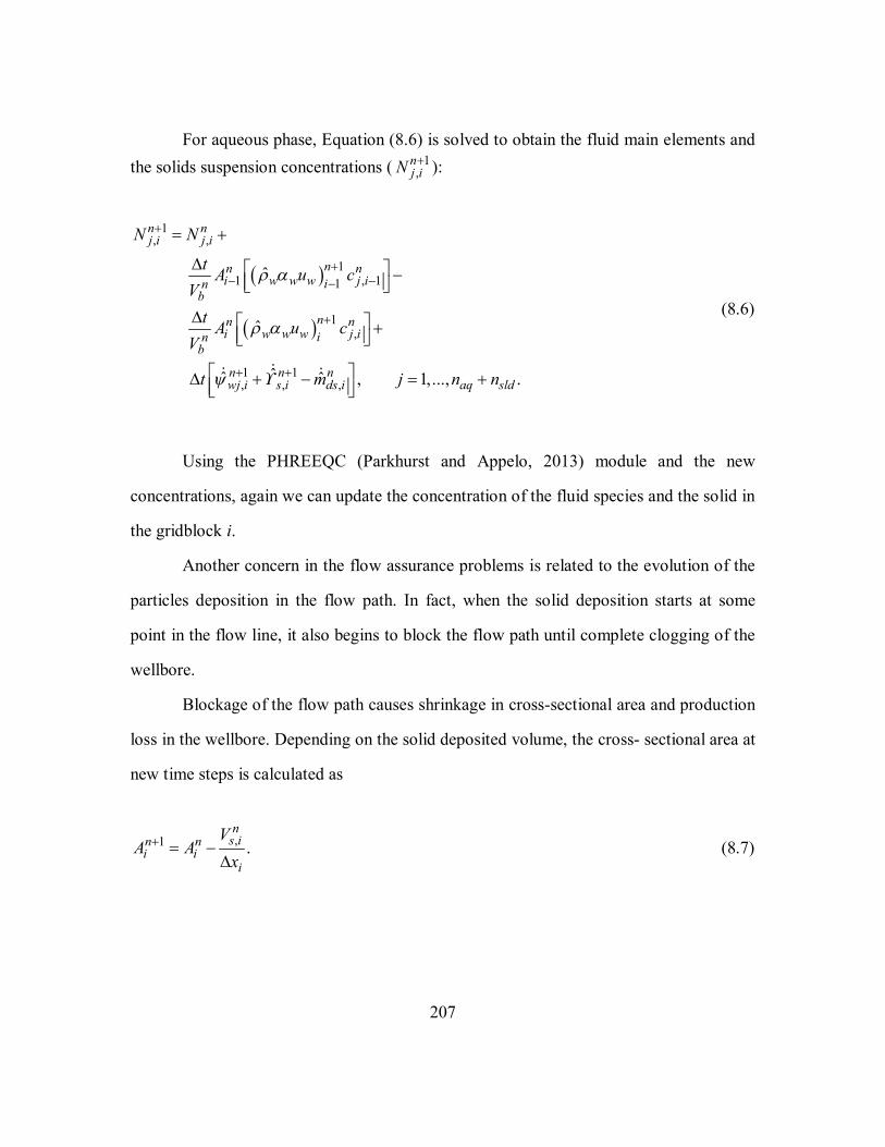
207
For aqueous phase, Equation (8.6) is solved to obtain the fluid main elements and the solids suspension concentrations ( 1
,n
j iN ):
1, ,
11 , 11
1,
1 1, , ,
ˆ
ˆ
ˆˆ ˆ , 1,..., .
n nj i j i
nn ni w w w j iin
b
nn ni w w w j iin
b
n n nwj i s i ds i aq sld
N N
t A u cV
t A u cV
t m j n n
(8.6)
Using the PHREEQC (Parkhurst and Appelo, 2013) module and the new
concentrations, again we can update the concentration of the fluid species and the solid in
the gridblock i.
Another concern in the flow assurance problems is related to the evolution of the
particles deposition in the flow path. In fact, when the solid deposition starts at some
point in the flow line, it also begins to block the flow path until complete clogging of the
wellbore.
Blockage of the flow path causes shrinkage in cross-sectional area and production
loss in the wellbore. Depending on the solid deposited volume, the cross- sectional area at
new time steps is calculated as
,1 .
ns in n
i ii
VA A
x (8.7)

208
Thus, using Equation (8.7), we can follow the progress of solid deposition in each
wellbore gridblock. When the cross-sectional area reaches to a point where the wellbore
flow starts to decline steeply, a remediation job should be started.
8.3 SIMULATIONS RESULTS IN STAND-ALONE WELLBORE MODEL
In the following sections, we describe the multiphase flow simulations in vertical
wells and in a horizontal pipeline to illustrate the implementation of different flow
assurance scenarios. The examples show how asphaltene can be generated in the wellbore
and be evolved along the well at different conditions, how wax is formed in the
horizontal pipelines at low temperatures, and how the geochemical scale reaction with
transportation can be coupled in the wells.
Appendices E.2 through E.4 show the sample input data for asphaltene, wax and
geochemical scale deposition simulations.
8.4 ASPHALTENE DEPOSITION
We considered three simulation examples in this part. First, we perform
simulation of asphaltene deposition in the wellbore with fluid Sample 1. In this case, we
reach the bubble point pressure of the fluid in the middle of the wellbore and have
concurrent flow of gas and liquid, plus asphaltene deposition. Second, we investigate the
effect of CO2 on asphaltene deposition in fluid Sample 1. This simulation can illustrate
the effect of CO2 on asphaltene deposition in the production well, after breakthrough of
CO2 in enhanced oil recovery.
Finally, we perform similar simulations for fluid Sample 2 which is oil heavier
than sample one and does not evaporate gas in the well.

209
8.4.1 Asphaltene Deposition Case Study with Fluid Sample 1
Table 8.1 shows the input parameters for this case. Tables 8.2 and 8.3 show the
composition of the fluid Sample 1, and the characterization of the fluid that are used for
our simulation study. The onset pressure and temperature data for the sample fluid one
are plotted with the vapor / liquid equilibrium line in Figure 8.1. Since we need to tune
the onset pressures and temperatures of asphaltene precipitation in our model, we used
those values as input data in our simulation.
In this case study, we have an 8000 ft well which is in primary production stage.
This well is in a reservoir with initial pressure of 5200 psi and operates with 1800 psi at
wellhead. We will perform multiphase flow simulation for this well to analyze its
performance for flow assurance issues. From Figures 8.2 and 8.3, we already know that
this well can be subjected to the asphaltene flow assurance problem. PVT analysis can
qualitatively show whether the asphaltene precipitation can occur or not. We solve the
steady-state solution of the well at initial time, and map it on the vapor/liquid equilibrium
and asphaltene onset curve shown in Figure 8.3. As we can see, the pressure-temperature
(P-T) path at initial condition (the blue dash line) moves from the asphaltene stable zone
to the asphaltene unstable zone and also to the two-phase region zone. Hence, with this
analysis, we understand that our well can potentially have asphaltene precipitation.
We proceed with the simulations for predicting the asphaltene deposition rate and
quantifying the amount of asphaltene precipitation in the well. Figure 8.4 shows the
asphaltene precipitation versus pressure for different temperatures. Since temperature
changes drastically in the wellbore, we can expect more asphaltene precipitation in the
upper part of the well, where the temperature of the wellbore is lower. As Figure 8.2
shows that the maximum asphaltene precipitation occurs around the bubble point
pressure, where the solubility of asphaltene is minimum. As a matter of fact, once gas is

210
relieved from the crude oil, asphaltene components become more stable and more soluble
in the oil.
Performing the simulation runs for the wellbore, we can obtain the magnitude of
asphaltene deposition and the rate of deposition in the wellbore. Asphaltene deposition in
the wellbore changes the wellbore cross-sectional area.
Figure 8.4 shows the profiles of inner radius of the well versus time. As can be
seen, the wellbore cross-section starts to shrink from the depth of 6650 ft, all the way to
the surface, and reaches the minimum diameter at 2777 ft. The surface of the precipitated
asphaltene has small dents due to removal of asphaltene by shear forces. Figure 8.5
shows the profiles of asphaltene flocculates in the wellbore. As we can observe, the
concentration of asphaltene reaches the maximum value at 2777 ft. This behavior justifies
the maximum deposition at that point.
Accumulation of asphaltene particles in the wellbore can consequently change the
pressure, temperature, and velocity fields profiles in the wellbore. Accordingly, it also
influences the amount of fluid influx from the reservoir. Asphaltene deposition
pressurizes the bottom-hole due to blockage of the wellbore and increment of friction
forces between the surfaces of deposited asphaltene and the moving fluid. Consequently,
asphaltene deposition reduces the influx from reservoir to the wellbore. Figures 8.6
through 8.9 show the pressure, temperature, oil velocity, and liquid velocity profiles at
different times.
Due to asphaltene deposition, velocity fields are drastically changed around the
largest deposited area in the wellbore. Velocity change can additionally affect the heat
exchange rate between the wellbore fluid and the surrounding. Figure 8.6 shows the
temperature of the fluid in the wellbore, which also decreases with progression of time.

211
Changes in the fluid temperature contradictorily increase the asphaltene precipitation and
decrease the asphaltene sticking probability on the well surface.
Moreover, Figure 8.10 shows the variation of pressure at bottom-hole with time.
Asphaltene particle blockage in the wellbore increases the pressure of bottom-hole with
time elapsed. As a consequence, Figure 8.11 shows that the flow rate of fluid decreases
with time due to less fluid influx from the reservoir.
8.4.2 Effect of CO2 on Asphaltene Deposition
Applications of CO2 and light hydrocarbon gas injections for enhanced oil
recovery process have introduced additional flow assurance issues into the reservoirs and
the wellbores (Tuttle, 1983). In several conventional oil fields in the Middle East,
asphaltene deposition has been reported as the most problematic issue during the CO2
flooding process.
In this section, we will simulate the effect of CO2 on asphaltene precipitation and
deposition in the wellbore. In fact, this simulation aims to capture the condition when
CO2 breakthroughs in the production well and mixes with the crude oil.
Vargas (2009) showed that existence of light components or contaminations in
crude oil changes the phase behavior of oil drastically. He showed asphaltene becomes
more unstable when natural gas or CO2 is mixed with oil. Figure 8.12 shows his results
for the effect of Methane, Nitrogen, and Carbon Dioxide on the P-T phase envelope of
crude oil. As we can see, the presence of light components can increase the bubble point
pressure and the onset pressure of asphaltene in the crude oil. Vargas (2009) used PC-
SAFT EOS to describe the effect of light components on asphaltene phase behavior.
Since in our asphaltene precipitation modeling approach we do not rigorously
include the effect of composition on the asphaltene onset pressure, we define those

212
pressures for different temperatures as input variables. In fact, since the cubic Equation-
of-State is tuned (for the binary interaction coefficients) to only one set of compositions
for the asphaltene precipitation, it might not be correct for the whole range of
compositions. However, using experimental values for asphaltene onset pressure can
reduce tuning errors for asphaltene precipitation models.
Table 8.4 illustrates the onset pressure of our synthetic fluid (Sample 1) for
different molar ratios of CO2 and oil mixture. The composition of oil after mixing with
CO2 has been shown in Table 8.5. The input onset pressures follow a similar trend as
Figure 8.12 (c). With the new compositions of the oil and the input onset pressures of
asphaltene, the amount of asphaltene precipitation can be calculated from our asphaltene
precipitation module. Figure 8.13 shows the amount of asphaltene precipitation for
different molar ratios of CO2 at 212 oF. The higher the content of CO2 the larger
asphaltene precipitation is obtained.
We performed multiphase flow simulations in the wellbore for 90 days with the
presence of considerable amount of CO2 in the reservoir fluid. We employed similar
input data in Section 8.5.1 for the wellbore and reservoir geometries. Figure 8.14 shows
the asphaltene concentration profiles for different compositions of the reservoir oil at the
end of 90 days. As we can see, asphaltene concentration is zero in the vicinity of the
perforations. Asphaltene starts to flash out from crude oil when pressure and temperature
are reduced in the upper parts of the wellbore. Comparing the asphaltene concentration
profiles for different compositions of CO2 in Figure 8.14, we observe that the existence of
larger amount of CO2 lowers the starting point of asphaltene precipitation in the wellbore.
Hence, in the cases where more CO2 reaches the production well, more asphaltene is
generated in the bottom of the well. Similarly, we compared the effect of CO2 on the
pressure, temperature, and gas volume fraction profiles in Figures 8.15 through 8.17. CO2

213
can indirectly change the pressure and temperature profiles by changing the velocity
fields in the wellbore. In addition, the flow regime change can also change the gas
volume fraction along the wellbore. As Figure 8.17 shows increment of CO2 percent in
the fluid mixture generally increases the gas volume fraction in the upper part of the
wellbore. However, the flow regime change in higher percent of CO2 can also affect the
gas volume fraction change in the wellbore.
Finally, we show the propagation of asphaltene deposition on the surface of the
wellbore in Figure 8.18. In the presence of CO2 wellbore can be plugged several times
faster than without CO2. In addition, the presence of CO2 lowers the maximum plugged
cross-section more toward the bottom of the well.
8.4.3 Asphaltene Deposition Case Study with Fluid Sample 2
In this section, we design another case that studies asphaltene deposition in the
wellbore in the absence of gas. Fluid Sample 2 was designed to show the effect of fluid
type on the propagation of asphaltene on the surface of the wellbore. In contrast to fluid
Sample 1, fluid Sample 2 does not evaporate gas in the wellbore. This fluid is heavier
than the previous fluid. Tables 8.6 and 8.7 show the fluid characterization and the
compositions, respectively. In comparison to fluid Sample 1, this fluid generates more
asphaltene at different temperatures as shown in Figure 8.19. In addition, since the bubble
point pressure of this fluid is very low, the trends of asphaltene precipitation curves are
different from that of fluid Sample 1.
We set the simulation input parameters of the wellbore and the reservoir, and the
operation condition of the well is given in Table 8.8. We perform the simulation for 90
days. Figure 8.20 shows the asphaltene flocculates and the transport coefficient profiles at

214
the end of simulation time. Since the precipitation of asphaltene starts from the bottom of
the well, asphaltene deposition covers all the parts in the well. However, since the
transport coefficient decreases in the upper part of the well, the deposition rate is smaller
in that part. Thus, as Figure 8.21 shows, the asphaltene particles are accumulated in the
bottom-hole.
8.5 WAX DEPOSITION
A horizontal pipeline with 1000 ft length as given in Table 8.9 is considered for
the simulation of wax deposition. In this case, we inject 0.2335 ft3/sec oil to the pipeline
and maintain the outlet pressure at 1000 psi. We perform the simulation for 10 days to
see how wax is generated and deposited in the pipeline.
Table 8.10 shows the injected fluid composition and the properties of the oil
mixture components. Using the wax phase behavior module in UTWELL, the calculated
Wax Appearance Temperature for this fluid is shown in Figure 8.22. As we can see, wax
is formed at very low temperatures in comparison to asphaltene.
Figures 8.23 through 8.25 show the wax deposition thickness, pressure and
temperature profile variations in the pipeline. The graphs show that wax is mostly
accumulated in the outlet of the pipeline where the temperature is the lowest. In fact, the
injected fluid has more time to exchange heat when it reaches the outlet. Recalling from
Chapter 7, wax deposition mechanism is highly dependent on the temperature gradient.
8.6 SCALE DEPOSITION
Simulation of scale deposition is considered in the wellbore by coupling
multiphase flow calculations in UTWELL and geochemical reactions calculations in

215
PHREEQC (Parkhurst and Appelo, 2013). Scale is usually formed when two
incompatible aqueous phases are mixed or when an ionic reaction happens in the
reservoir. In such situations, geochemical scales can flocculate from reservoir and entrain
to the wellbore. Like other solid particles, geochemical solid scales can generate a cluster
of solids which can deposit in a similar mechanism on the surface of the wellbore.
In this section, we considered a 5000 ft well to simulate scale deposition in the
wellbore. We assume that our well produces water and oil with the productivity indices
shown in Table 8.11. Other pertinent data also have been shown in Table 8.11. We also
presume that the aqueous phase contains 0.1 mole/kg of Anhydrite solid, and 0.1 mole/kg
of non-reacted sulfate and calcium ions.
Figure 8.26 shows the transport coefficient and scale flocculate concentration
profiles after 90 days. Figure 8.27 shows the scale deposition thickness in the wellbore
with elapsed time. As can be seen, from bottom of the well to the top, scale is mostly
deposited in the bottom of the well. In contrast to asphaltene and wax depositions,
geochemical scale is mostly deposited in the bottom of the well, where the concentration
and the transport coefficients are the largest.

216
Table 8.2 Fluid characterization and composition for fluid Sample 1
Component Pc (psi) Tc ( R ) VC (ft3/lbmol) Mw (lb/lbmol) Acentric Factor Parachor Volume
Shift Primary
Composition CO2 1070.09 547.56 1.5071 44.01 0.225 168.17 0 0.0246 C1-C2 668.51 360.61 1.6431 17.417 0.015127 92.19 0 0.4041 C3-C5 573.15 732.89 3.8098 53.516 0.179313 195.33 0 0.0755 C6-C19 291.41 1135.31 13.7197 164.423 0.655007 512.21 0 0.2719 C20-C30 175.41 1419.29 29.033 340.927 1.064023 1016.51 0 0.1064 C31+ 143.17 1682.93 56.5489 665.624 1.371778 1944.21 0 0.0774 Asphaltene 143.17 1682.93 56.5489 665.624 1.371778 1944.21 0 0.0401
Table 8.1 Input parameters for simulation of asphaltene deposition in the wellbore with fluid Sample 1
Well Data Reservoir and Fluid Data
Well MD 8000 ft Net pay zone 200 ft Well TVD 8000 ft Reservoir pressure 5200 psi Max grid size 50.0 ft Reservoir temperature 212 oF Ambient temperature at top 60 oF Ambient temperature at bottom 212 oF Total heat transfer coefficient 1.0 Btu/ft2-hr-oF Tubing ID 0.229 ft Oil productivity index 0.2 ft3/psi-ft-day Water productivity index 0.0 ft3/psi-ft-day Gas productivity index 0.0 ft3/psi-ft-day Wellhead pressure 1800 psi
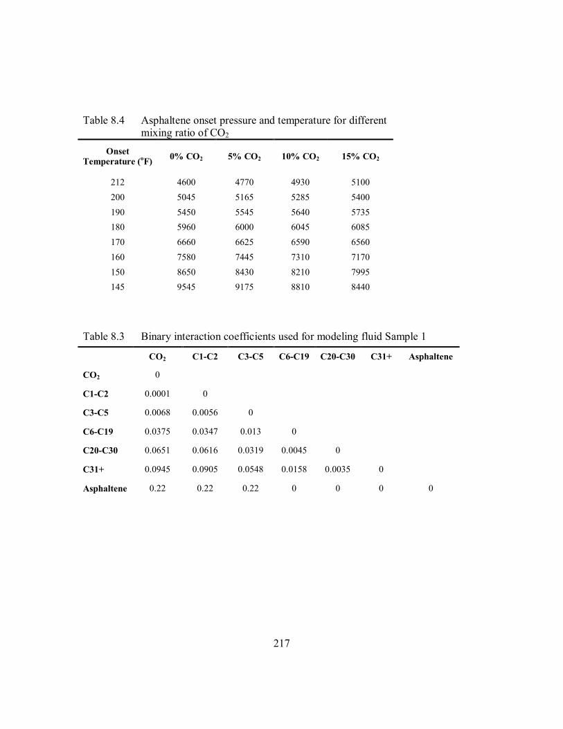
217
Table 8.4 Asphaltene onset pressure and temperature for different mixing ratio of CO2
Onset Temperature (oF) 0% CO2 5% CO2 10% CO2 15% CO2
212 4600 4770 4930 5100 200 5045 5165 5285 5400 190 5450 5545 5640 5735 180 5960 6000 6045 6085 170 6660 6625 6590 6560 160 7580 7445 7310 7170 150 8650 8430 8210 7995 145 9545 9175 8810 8440
Table 8.3 Binary interaction coefficients used for modeling fluid Sample 1
CO2 C1-C2 C3-C5 C6-C19 C20-C30 C31+ Asphaltene
CO2 0
C1-C2 0.0001 0
C3-C5 0.0068 0.0056 0
C6-C19 0.0375 0.0347 0.013 0
C20-C30 0.0651 0.0616 0.0319 0.0045 0
C31+ 0.0945 0.0905 0.0548 0.0158 0.0035 0
Asphaltene 0.22 0.22 0.22 0 0 0 0

218
Table 8.5 Reservoir fluid composition for different mixing ratio of CO2
Component 0% CO2 5% CO2 10% CO2 15% CO2
CO2 0.0246 0.07337 0.12214 0.17091 C1-C2 0.4041 0.383895 0.36369 0.343485 C3-C5 0.0755 0.071725 0.06795 0.064175 C6-C19 0.2719 0.258305 0.24471 0.231115 C20-C30 0.1064 0.10108 0.09576 0.09044 C31+ 0.0774 0.07353 0.06966 0.06579 Asphaltene 0.0401 0.038095 0.03609 0.034085
Table 8.6 Fluid characterization and composition for fluid Sample 2
Component Pc (psi) Tc ( R ) VC (ft3/lbmol) Mw (lb/lbmol) Acentric Factor Parachor Volume
Shift Primary
Composition N2-C1 640.75 324.04 1.56 17.93 0.01 71.32 0 0.0000321 CO2 1069.87 547.56 1.51 44.01 0.23 78 0 0.0000409 C2-C3 647.74 630.39 2.94 39.45 0.13 136.05 0 0.0175432 IC4-NC5 519.73 796.06 4.46 64.55 0.21 206.67 0 0.1114261 C6-C9 405.61 1067.24 7.33 124.49 0.33 337.4 0 0.3627861 C10-C19 274.6 1314.89 12.27 217.81 0.57 604.02 0 0.3516170 C20-C29 191.16 1557.76 18.8 364.18 0.89 1022.21 0 0.1154219 C30+ 128.27 1859.46 27.68 622.54 1.26 1760.39 0 0.0411327

219
Table 8.7 Binary interaction coefficients for modeling fluid Sample 2
N2-C1 CO2 C2-C3 IC4-NC5 C6-C9 C10-C19 C20-C29 C30+
N2-C1 0
CO2 0.13000 0 C2-C3 0.00776 0.13500 0
IC4-NC5 0.02109 0.12500 0.00336 0
C6-C9 0.04493 0.10146 0.01600 0.00477 0
C10-C19 0.07788 0.10146 0.03853 0.01963 0.00515 0 C20-C29 0.11049 0.10146 0.06372 0.03907 0.01704 0.00353 0
C30+ 0.15119 0.11335 0.09612 0.06530 0.03542 0.01348 0.00308 0
Table 8.8 Input parameters for simulation of asphaltene deposition in the wellbore with fluid Sample 2
Well Data Reservoir and Fluid Data
Well MD 8000 ft Net pay zone 100 ft Well TVD 8000 ft Reservoir pressure 5000 psi Max grid size 50.0 ft Reservoir temperature 220 oF Ambient temperature at top 60 oF Ambient temperature at bottom 220 oF Total heat transfer coefficient 1.0 Btu/ft2-hr-oF Tubing ID 0.229 ft Oil productivity index 0.2 ft3/psi-ft-day Water productivity index 0.0 ft3/psi-ft-day Gas productivity index 0.0 ft3/psi-ft-day Wellhead pressure 2000 psi

220
Table 8.9 Input parameters for simulation of wax deposition in a pipeline
Pipe Data
Well MD 1000 ft Well TVD 0.0 ft Max grid size 50.0 ft Surrounding temperature 40 oF Total heat transfer coefficient 20.0 Btu/ft2-hr-oF Pipe inner diameters 0.229 ft Oil injection rate 0.2335 ft3/sec Outlet pressure 1000 psi
Table 8.10 Fluid characterization and composition for wax crude oil sample
Component Pc (psi) Tc ( R ) VC (ft3/lbmol) Mw (lb/lbmol) Acentric Factor
Primary Composition
C1 667.1961 343.08 1.60823 16.043 8.00E-03 0.6 C2 708.3447 549.72 2.404223 30.07 9.80E-02 0.1 NC4 551.0981 765.36 4.142411 58.124 0.193 0.05 NC5 489.3751 845.28 4.938403 72.151 0.251 0.05 FC6 477.0305 913.5 5.588193 86 0.27504 0.05 FC14 284.0727 1261.26 11.74495 190 0.604823 0.05 FC17 240.2788 1348.56 14.36036 237 0.72857 0.05 FC33 137.5541 1609.02 24.62704 426 1.143446 0.05

221
50 100 150 200 250 3002000
3000
4000
5000
6000
7000
8000
9000
10000
Pres
sure
[psi
]
Temperature [oF]
Calculated VLEInput Upper AOP
Figure 8.1 Asphaltene vapor / liquid saturation line and asphaltene onset pressure line for fluid Sample 1.
Table 8.11 Input parameters for simulation of scale deposition in the wellbore
Well Data Reservoir and Fluid Data
Well MD 5000 ft Net pay zone 150 ft Well TVD 5000 ft Reservoir pressure 2500 psi Max grid size 50.0 ft Reservoir temperature 180 oF Ambient temperature at top 60 oF Oil API gravity 30 Ambient temperature at bottom 180 oF Oil bubble point pressure 500 psi Total heat transfer coefficient 1.0 Btu/ft2-hr-oF Gas specific gravity 0.55 Tubing ID 0.229 ft Water specific gravity 1.0 Oil productivity index 0.5 ft3/psi-ft-day Gas heat capacity 0.55 Btu/lbm-oF Water productivity index 0.1 ft3/psi-ft-day Oil heat capacity 0.45 Btu/lbm-oF Gas productivity index 0.0 ft3/psi-ft-day Water heat capacity 1.0 Btu/lbm-oF Wellhead pressure 500 psi Geochemical scale type Anhydrite

222
0 2000 4000 6000 80000
0.5
1
1.5
2
2.5
3
3.5
Asp
halte
ne P
reci
pita
tion
[wt%
]
Pressure [psi]
T = 212 oF
T = 180 oF
T = 160 oF
Figure 8.2 Weight percent of asphaltene precipitation as function of pressure in different temperatures.
50 100 150 200 250 3001000
2000
3000
4000
5000
6000
7000
Pres
sure
[psi
]
Temperature [oF]
Calculated VLEInput Upper AOPP-T Route
Two-phase Region
AsphalteneStable Zone
Figure 8.3 Pressure and temperature route from bottom of the well to the surface at time zero (blue dash line), asphaltene onset pressure (red dots) and fluid saturation line (solid line).

223
0 0.02 0.04 0.06 0.08 0.10
1000
2000
3000
4000
5000
6000
7000
8000
Dep
th [f
t]
Asphaltene Thickness [ft]
0.0 day20 days45 days60 days90 days
Figure 8.4 Thickness of asphaltene deposit on the inner surface of the wellbore for different times.
0 0.2 0.4 0.6 0.8 1 1.2 1.40
1000
2000
3000
4000
5000
6000
7000
8000
Casph [10-3 lbmol/ft3]
Dep
th [f
t]
0.0 day20 days45 days60 days90 days
Figure 8.5 Asphaltene flocculate concentration profiles in the wellbore for different times.

224
190 195 200 205 210 2150
1000
2000
3000
4000
5000
6000
7000
8000
Dep
th [f
t]
Temperature [oF]
0.0 day20 days45 days60 days90 days
Figure 8.6 Temperature profiles for different times during asphaltene deposition in the wellbore.
1000 2000 3000 4000 5000 60000
1000
2000
3000
4000
5000
6000
7000
8000
Dep
th [f
t]
Pressure [psi]
0.0 day20 days45 days60 days90 days
Figure 8.7 Pressure profiles for different times during asphaltene deposition in the wellbore.

225
0 2 4 6 8 10 12 140
1000
2000
3000
4000
5000
6000
7000
8000
Dep
th [f
t]
Oil Superficial Velocity [ft/sec]
0.0 day20 days45 days60 days90 days
Figure 8.8 Oil superficial velocity profiles for different times in the wellbore during asphaltene deposition in the wellbore.
0 0.5 1 1.5 20
1000
2000
3000
4000
5000
6000
7000
8000
Dep
th [f
t]
Gas Superficial Velocity [ft/sec]
0.0 day20 days45 days60 days90 days
Figure 8.9 Gas superficial velocity profiles for different times in the wellbore during asphaltene deposition in the wellbore.

226
0 20 40 60 80 1005050
5060
5070
5080
5090
5100
Bot
tom
-hol
e Pr
essu
re [p
si]
Time [day]
Figure 8.10 Variation of bottom-hole pressure due to asphaltene deposition with time elapsed.
0 20 40 60 80 1004000
4500
5000
5500
6000
Oil
Flow
Rat
e [b
bl/d
ay]
Time [day]
Figure 8.11 Variation of oil flow rate due to asphaltene deposition with time progression.

227

228
Figure 8.12 Effect of light hydrocarbons mixing on the stability of asphaltene in crude oil. (a) Effect of Methane, (b) effect of Nitrogen (c) effect of CO2 (from Vargas (2009)).
1000 2000 3000 4000 5000 60000
0.2
0.4
0.6
0.8
1
1.2
1.4
Asp
halte
ne P
reci
pita
tion
[wt%
]
Pressure [psi]
0% CO2
5% CO2
10% CO2
15% CO2
Figure 8.13 Weight percent of asphatlene precipitation in presence of CO2 with different molar ratios at 212 oF.

229
0 0.5 1 1.50
1000
2000
3000
4000
5000
6000
7000
8000
Dep
th [f
t]
Casph [10-3 lbmol/ft3]
0% CO2
5% CO2
10% CO2
15% CO2
Figure 8.14 Asphaltene concentration profiles at the end of 90 days of production in the wellbore for different fluid compositions.
1000 2000 3000 4000 5000 60000
1000
2000
3000
4000
5000
6000
7000
8000
Dep
th [f
t]
Pressure [psi]
0% CO2
5% CO210% CO2
15% CO2
Figure 8.15 Pressure profiles at the end of 90 days of production in the wellbore for different fluid compositions.

230
170 180 190 200 210 2200
1000
2000
3000
4000
5000
6000
7000
8000
Dep
th [f
t]
Temperature [oF]
0% CO2
5% CO210% CO2
15% CO2
Figure 8.16 Temperature profiles at the end of 90 days of production in the wellbore for different fluid compositions.
0 0.05 0.1 0.15 0.20
1000
2000
3000
4000
5000
6000
7000
8000
Dep
th [f
t]
Gas Volume Fraction
0% CO2
5% CO210% CO2
15% CO2
Figure 8.17 Gas volume fraction profiles at the end of 90 days of production in the wellbore for different fluid compositions.
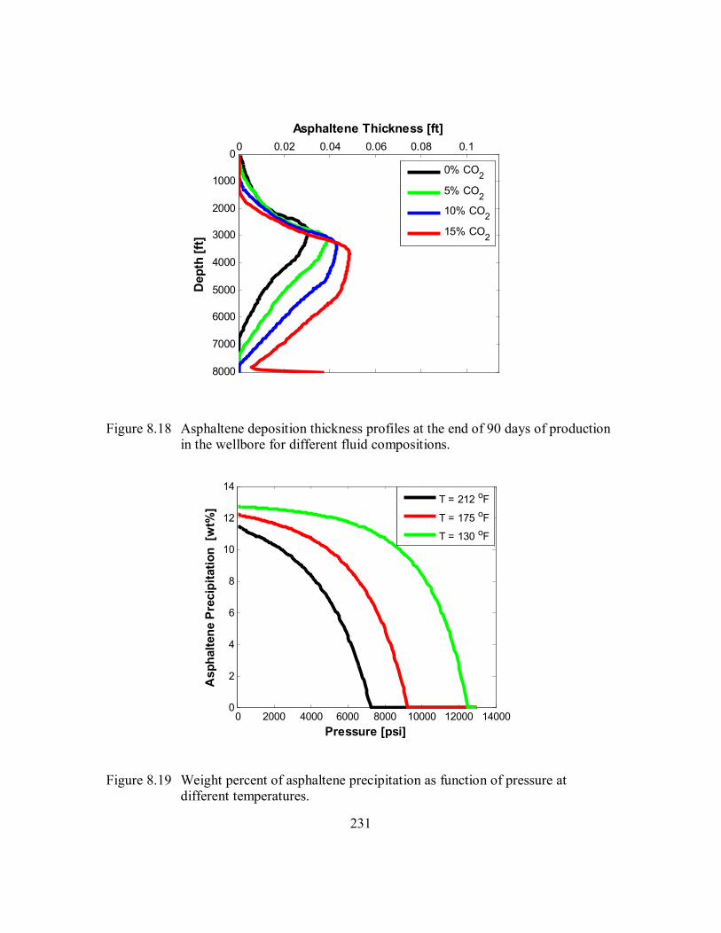
231
0 0.02 0.04 0.06 0.08 0.10
1000
2000
3000
4000
5000
6000
7000
8000
Dep
th [f
t]
Asphaltene Thickness [ft]
0% CO2
5% CO210% CO2
15% CO2
Figure 8.18 Asphaltene deposition thickness profiles at the end of 90 days of production in the wellbore for different fluid compositions.
0 2000 4000 6000 8000 10000 12000 140000
2
4
6
8
10
12
14
Asp
halte
ne P
reci
pita
tion
[wt%
]
Pressure [psi]
T = 212 oF
T = 175 oF
T = 130 oF
Figure 8.19 Weight percent of asphaltene precipitation as function of pressure at different temperatures.
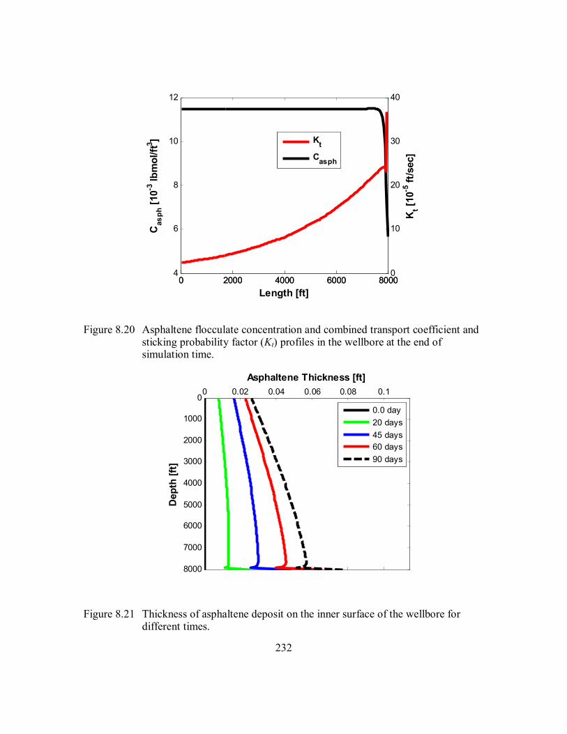
232
0 2000 4000 6000 80004
6
8
10
12
Cas
ph [1
0-3 lb
mol
/ft3 ]
0 2000 4000 6000 80000
10
20
30
40
Kt [1
0-5 ft
/sec
]
Length [ft]
KtCasph
Figure 8.20 Asphaltene flocculate concentration and combined transport coefficient and sticking probability factor (Kt) profiles in the wellbore at the end of simulation time.
0 0.02 0.04 0.06 0.08 0.10
1000
2000
3000
4000
5000
6000
7000
8000
Dep
th [f
t]
Asphaltene Thickness [ft]
0.0 day20 days45 days60 days90 days
Figure 8.21 Thickness of asphaltene deposit on the inner surface of the wellbore for different times.

233
60 70 80 90 100 110 120 1300
1000
2000
3000
4000
5000
6000
Pres
sure
[psi
]
Temperature [oF]
Figure 8.22 Wax appearance temperature (WAT) for different pressures.
0 200 400 600 800 10000
0.2
0.4
0.6
0.8
1
Wax
Thi
ckne
ss [m
m]
Length [ft]
0.0 day4 days7 days10 days
Figure 8.23 Thickness of wax deposit on the inner surface of the pipeline for different times.

234
0 200 400 600 800 10001000
1002
1004
1006
1008
1010
1012
1014
1016
1018
Pres
sure
[psi
]
Length [ft]
0.0 day4 days7 days10 days
Figure 8.24 Pressure profile in the pipeline for different simulation times.
0 200 400 600 800 100046
48
50
52
54
56
58
60
Tem
pera
ture
[o F]
Length [ft]
0.0 day4 days7 days10 days
Figure 8.25 Temperature profiles in the pipeline for different simulation times.

235
0 1000 2000 3000 4000 500020
40
60
80
100
120
Csc
ale [1
0-3 m
ol/k
g]
0 1000 2000 3000 4000 50000
2
4
6
8
10
Kt [1
0-10 ft
/sec
]
Length [ft]
KtCscale
Figure 8.26 Geochemical scales flocculate concentration and combined transport coefficient and sticking probability factor (Kt) profiles in the wellbore at the end of simulation time.
0 0.02 0.04 0.06 0.08 0.10
1000
2000
3000
4000
5000
Dep
th [f
t]
Scale Deposition Thickness [ft]
0.0 day20 days45 days60 days90 days
Figure 8.27 Thickness of scale deposit on the inner surface of the wellbore for different times.

236
Chapter 9: Coupled Wellbore Reservoir Model
In this chapter, we introduce a compositional wellbore model coupled to a
compositional reservoir simulator to study the transport phenomena in an entire
subsurface system. In previous chapters, we introduced a compositional standalone
wellbore model along with flow assurance modules for asphaltene, wax, and geochemical
scales.
Since in the reservoir the pressure and temperature do not change significantly,
flow assurance problems might not be observed as readily as in a wellbore. However,
some field reports have shown that asphaltene deposition and geochemical scales
formation can occur at certain conditions in the reservoirs. During miscible gas flooding,
such as CO2 injection for an enhanced oil recovery process, asphaltene precipitation can
occur at the reservoir condition. Asphaltene precipitation may plug the pores, change the
porosity and the permeability in reservoirs, alter rock wettability and affect all aspects of
oil production, processing, and transportation in the reservoir. Incompatible water mixing
in the formation, during the secondary recovery, is also believed to be one of the main
sources of triggering scale precipitations in the reservoirs. Likewise, geochemical scales
can plug the near wellbore regions and reduce the productivity of the wells.
In the following sections, we discuss coupling of UTWELL to UTCOMP (Chang
1990, in house compositional reservoir simulator developed at UT Austin, Appendix A)
to solve the wellbore/reservoir model. We also discuss the solution procedures for
coupling schemes and present several case studies for asphaltene deposition model in the
reservoir and in the wellbore.

237
9.1 A REVIEW OF COUPLED WELLBORE RESERVOIR MODELS
For a comprehensive reservoir production simulation, the development and
application of a coupled wellbore-reservoir simulator is essential. A coupled wellbore-
reservoir simulator can be applied to different problems either in the production or in the
reservoir engineering areas. For instance, in the well test analysis, wellbore damage
simulation (i.e., wellbore plugging by precipitates), well design (i.e., smart wells
application), well performance analysis and well control (i.e., kick and blowout
situation), a dynamic wellbore-reservoir simulator is required. Several researchers have
recently introduced coupled wellbore-reservoir models using different mechanistic
approaches. In this section, we review what we consider to be the most important
published works.
Stone et al. (1989) presented a fully implicit, blackoil and three-dimensional
reservoir simulator coupled to a blackoil and one-dimensional wellbore simulator. They
mainly targeted a horizontal well for wellbore-reservoir system in their study. They also
used two-fluid model considering different flow regimes for the wellbore model. Stone et
al. (1989) solved oil, water and gas mass balance, liquid/gas momentum balance energy
equation simultaneously with reservoir equations in their model. They also considered
parallel flow in the inner tubing and outer annuli and slant angle effect. Stone et al.
(1989) validated their model against field data and showed a good agreement between
their model results and field data.
Hasan and Kabir (1996), and Hasan et al. (1997; 1998) presented a blackoil model
for single and two-phase flow in wellbores coupled to the reservoir. They applied a
hybrid numerical model for the wellbore and an analytical single-phase model for the
reservoir. Material balances for each phase, one momentum balance equation for the
mixture and energy balance were solved to obtain pressure, velocity, temperature, and

238
fluid density in the wellbore. To calculate the liquid fraction (holdup) at each segment of
the wellbore, Hasan et al. (1998) tracked the migration of gas bubbles throughout the
wellbore. They used the wellbore-reservoir model for well test analysis application.
Likewise, Fan et al. (2000) developed a semi-analytical wellbore-reservoir
simulator in which a single-phase analytical model for the reservoir was coupled to the
wellbore. Fan et al. (2000) mainly targeted thermal effects in their study and applied the
simulator to a high-temperature gas well pressure buildup test.
Recently, more comprehensive compositional wellbore-reservoir models have
been introduced by different researchers. Pourafshary et al. (2009) presented
development of a thermal compositional coupled wellbore-reservoir simulator. He
performed simulation on producing well with different case studies for crude oil,
condensate gas and volatile oil. He demonstrated that the blackoil approach was not
accurate for the representation of condensate and volatile oils flow in the wellbore.
Livescu et al. (2009) also developed a fully-coupled thermal compositional
wellbore model. Mass conservation for each component, momentum conservation, and
energy equation for the mixture of the fluids were solved to obtain pressure, temperature,
and holdup profiles in the complete flow line. They used the drift-flux model to consider
the slippage between the phases. In their study, different cases for thermal process and
different well geometries were presented.
Shirdel (2010) also developed compositional wellbore model for the horizontal,
deviated and vertical wells. He showed the effect of pressure and temperature distribution
of horizontal wells on the productivity of the well in the reservoir simulators. He also
discussed that ignoring the pressure drop in the horizontal wells can cause erroneous
results for the production rates at the early stage of production.

239
9.2 METHODS OF COUPLING WELLBORE TO THE RESERVOIR
In the literature, two different approaches have been introduced for wellbore /
reservoir coupling. One method is an iterative explicit coupling, where the wellbore and
reservoir systems are solved separately. The other method fully couples the wellbore and
reservoir systems.
In the iterative method, the reservoir and wellbore pressure results are iteratively
conveyed to each system, along with calculation of productivity indices, to obtain the
influx/outflux rates to the wellbore. One of the advantages of the iterative coupling is that
the wellbore model can be coupled to any reservoir simulator.
In fully coupled wellbore-reservoir simulations, wellbore and reservoir models are
simultaneously solved. Behie et al. (1985) explained a mathematical approach to solve a
modified Jacobian matrix in the case where the well crosses multiple blocks of the
reservoir grid. They did not present the wellbore model to calculate the perforation
pressure. However, they discussed a method to implement a fully coupled wellbore-
reservoir system. They claimed that the fully coupled method was more stable than an
explicit wellbore pressure coupling.
In our study, since we developed the wellbore model as a standalone simulator,
we apply explicit coupling scheme for our wellbore/reservoir model. The flow chart
shown in Figure 9.1 shows the subroutines in the main program of UTCOMP (the
reservoir simulator) and the inclusion of UTWELL calculations. As can be seen, the
communicating parameter between wellbore and the reservoir is the rate for mass
influx/out-flux.
In Chapter 3, we defined the influx parameters in mass conservation equations as jk , which is the component k in phase j mass flux per unit length of the cell. This
parameter is calculated as below:

240
( ). kj j kj res
jjk
MwPI x P PMw
(9.1)
jPI in Equation (9.1) is the productivity index of each phase (water, oil and gas).
Appendix A explains the detail of well models and productivity index calculation in
UTCOMP. This parameter is obtained from a user specified value in input file in the
standalone wellbore model or calculated as follows for coupled wellbore/reservoir model:
2
,(0.15802)
x yj
o
w
k k zPI
rln Sr
(9.2)
where, or is the equivalent radius of well block which is calculated by either Peaceman
(1983) or Babu and Odeh’s (1989) models for vertical and horizontal wells, xk and yk
are the permeability in x and y directions, z is the grid block size, wr is the wellbore
size in perforation zone, and S is the skin factor. Asphaltene plugging in the perforation
zones, also changes wr in the productivity index calculation.
Other concerns remaining in explicit coupling of UTWELL to UTCOMP are the
time-step sizing and tight coupling for the convergence of both systems. Since the time-
step sizes in the transient wellbore models are very small (in order of several seconds) in
comparison to the reservoir models, synchronization between these two domains is
necessary. For this purpose, an additional criterion is included in the time-step control
method of both models to select the minimum time-step sizes of all calculations. Thus,
for the coupled transient wellbore model time-step sizes are in the order of several
seconds at the beginning of the simulation.

241
Moreover, for steady-state wellbore model coupling, an iterative solution must be
used to march large time-step sizes in the simulation. UTCOMP is an Implicit Pressure
and Explicit Concentration (IMPEC) simulator and solves the pressure equation with one
iteration. For this reason, convergence issues may occur if the wellbore model is not
tightly coupled. In our tight coupling, we perform iterations for pressure solution with the
new feeds of wellbore model. In fact, the solution of wellbore model changes the bottom-
hole pressure of the well and the amount of influx. Several iterations should be performed
until complete convergence is observed for both wellbore and reservoir systems mass
influx/outflux. Our experience shows that without tight coupling the reservoir time-steps
should be very small to overcome the numerical instabilities. Otherwise, oscillatory
results are obtained, which may stop the simulation later. Figure 9.2 shows the
comparison of iteratively coupled wellbore model and non-iteratively coupled wellbore
model for oil rate. As can be seen, with tight coupling the oscillatory results are
diminished.
9.3 COUPLED WELLBORE / RESERVOIR MODEL RESULTS
In this section, we present two case studies to show the simulation of asphaltene
deposition in a coupled wellbore / reservoir model. In the first case, we assume a scenario
that asphaltene is not formed in the reservoir and it is only precipitated in the wellbore. In
the second case, we use a version of UTCOMP that has asphaltene deposition module
(Darabi et al., 2012) and assumes asphaltene is deposited in the reservoir and the
wellbore.

242
9.3.1 Asphaltene Deposition Case One
In this case, the fluid composition and reservoir condition are properly chosen to
avoid asphaltene precipitation in the reservoir and near-wellbore. Table 9.1 illustrates the
configuration of the well and reservoir setup. Fluid composition is similar to the one in
Section 8.5.3. For the given fluid type, the asphaltene onset pressure at the reservoir
temperature, 220 oF, is 7250 psi. Hence, we expect the precipitation and deposition of
asphaltene to be initiated inside the wellbore, where the pressure and temperature decline
below the reservoir condition.
Furthermore, we assume a vertical well with 6000 ft depth which produces at a
constant wellhead pressure of 5200 psi (Table 9.1). We keep the wellhead pressure large
enough to make sure that reservoir pressure does not go below the onset pressure. We
perform the simulation for 100 days and monitor the results in the wellbore. Figure 9.3
shows the pressure and temperature route for different time-steps along the well. As can
be seen the bottom-hole pressure of the well is always above the onset pressure line and
increases with time and when we go further toward the wellhead, the pressure and
temperature decline in a way that fluid invades to asphaltene unstable zone. In most parts
of the well, we expect asphaltene deposition in this system. Once asphaltene destabilized
in the fluid, it begins to precipitate and aggregate where it can become large enough to
diffuse toward the well surface. As discussed previously, the amount of asphaltene
particle concentration, the transport coefficient, and sticking factor are the deriving forces
for deposition rate in the deposition models. These parameters are non-linearly coupled
functions of temperature, velocity, and pressure fields. Hence, we expect non-uniform
deposition rate profile in the well from bottom to the top of the well.
Figure 9.4 shows snap shots of the evolution of asphaltene solid deposition in the
wellbore in different time-steps. As can be seen, our simulation results can capture how

243
asphaltene is accumulated in the wellbore and build up starting from a particular point in
the well. This figure confirms our expectation that at a depth of about 4000 ft we have
maximum accumulation of asphaltene. Asphaltene accumulation smoothly reduces in the
upper part of the wells where we have less adhesion force and more drag force, which
facilitates the asphaltene detachment from the well surface.
Figure 9.5 also shows the oil flow rate in our well versus time. This figure
compares the productivity of the well, producing the same fluid if asphaltene was not
destabilized (became unstable) and blocked the well. As can be seen, asphaltene blockage
has significantly reduced the oil rate and decreased the productivity of the well.
9.3.2 Asphaltene Deposition Case Two
We selected fluid sample similar to Section 8.5.1 for this case. Table 9.2 shows
the main parameters of the wellbore and reservoir configuration setup. Appendix E.5 also
shows the sample input data for the coupled wellbore reservoir model. In contrast to
previous case in Section 9.2.1, we lower the pressure of the wellbore to below the bubble
point pressure of the fluid (2900 psi at 212 oF) and maintain the wellhead pressure at
1000 psi. We perform the simulation for 50 days to monitor the asphaltene deposition and
transportation in the wellbore and reservoir.
Figure 9.6 shows the propagation of pressure profile in the reservoir at the early
stage of the production. As can be seen, reservoir pressure declines from 5000 psi the
initial pressure in the area far from producer to 3116 psi near the well bottom-hole
pressure in the producer. Since the pressure in the near-wellbore reaches to the value
below asphaltene onset pressure, asphaltene components are stripped out in this area and
begin to deposit on the surface of the rock. Figures 9.7 and 9.8 show the concentration of
the precipitated asphaltene in the near wellbore and the amount of deposited asphaltene.

244
Within 50 days of production, about 100 ft of around wellbore area is damaged with
asphaltene precipitation. Although in this time period the amount of deposited asphaltene
is small but with time progression asphaltene precipitates can accumulate more in these
blocks.
Figure 9.9 shows the production rates for oil, water and gas, respectively. The
fluid production rates are declined fast due to a low pressure that we assign to the
wellhead. Additionally, once the reservoir starts to deplete the fluids, its pressure also
decline as shown in Figure 9.10. Due to the average reservoir pressure decline, plus the
blockage of the bottom-hole area and the near wellbore zone, the bottom-hole pressure
(Pbh) increases as shown in Figure 9.11. Bottom-hole pressure reaches to below the
bubble-point pressure from the beginning of the production. Hence, we always observe
two-phase flow in the wellbore.
The pressure and temperature path in the wellbore (Figure 9.12) shows that
asphaltene components can be stabilized in the crude oil with moving to the upper part of
the well. When more gas is released from oil, the solubility of oil increases and dissolves
the asphaltene components. Figure 9.13 shows the concentration of asphaltene
flocculates. As can be seen, above the depth of 3500 ft asphaltene disappears from oil and
dissolves back in the oil.
Finally, Figure 9.14 shows the deposition of asphaltene in the wellbore. Since
most of the precipitated asphaltene are available in the bottom of the well and the flow
rate is the lowest there, asphaltene mostly settles in the bottom of the well. As we
discussed earlier, the deposited asphaltene in the perforation zone decrease the
productivity index of the well.

245
Table 9.1 Input parameters for simulation case one of asphaltene deposition in the coupled wellbore/reservoir system
Reservoir dimension 4080ft 4080ft4080ft Fluid composition N2-C1 = 0.0000321 Gridblocks 51513 CO2 = 0.0000409
Area 382 acre C2-C3 = 0.0175432
Reservoir initial pressure 8000 psi IC4-NC5 = 0.1114261
Reservoir initial saturation 0.17 C6-C9 = 0.3627861
Reservoir temperature 220 oF C10-C19 = 0.3516170
Reservoir permeability 10 md C20-C29 = 0.1154219
Wellbore pressure 5200 psi C30+ = 0.0411327
Wellbore depth 6000 ft Wellbore diameter 0.2 ft Well roughness 0.0008
Table 9.2 Input parameters for simulation case two of asphaltene deposition in the coupled wellbore/reservoir system
Reservoir dimension 400ft 400ft60ft Fluid composition CO2 = 0.0246 Gridblocks 20203 C1-C2 = 0.4041
Area 3.67 acre C3-C5 = 0.0755
Reservoir initial pressure 5000 psi C6-C19 = 0.2719
Reservoir initial saturation 0.2 C20-C30 = 0.1064
Reservoir temperature 220 oF C31+ = 0.0774
Reservoir permeability 500 md Asphaltene = 0.0401
Wellbore pressure 1000 psi Wellbore depth 5000 ft Wellbore diameter 0.229 ft Well roughness 0.0008

246
Iter
atio
n
.
Figure 9.1 The sequence of subroutines in the UTCOMP and inclusion of UTWEL calculation (red boxes). The iteration is used for tight coupling of UTWELL and UTCOMP.
INITIALIZATION
DEFINE I/O FILES
WELLFACT
REGISTER UTWELL
AUTODT
SYNC WELL RES
UTWELL
RATES
SOLVER
ITIME = ITIME +1

247
0 1 2 3 4 5400
600
800
1000
1200
1400
1600
Oil
Flow
Rat
e [S
TB/D
ay]
Time [Day]
non-iteativeiterative
Figure 9.2 Comparison of an example rate solution for iterative and non-iterative coupling approaches in wellbore/reservoir system.
100 120 140 160 180 200 2205000
5500
6000
6500
7000
7500
8000
8500
9000
9500
Pres
sure
[psi
]
Temperature [oF]
Initial Condition23 days53 days77 daysOnset Pressure
Figure 9.3 Pressure and temperature route in the wellbore for different time-steps.

248
0 0.02 0.04 0.06 0.08 0.10
1000
2000
3000
4000
5000
6000
Dep
th [f
t]
Asphaltene Thickness [in]
0.0 day20 days45 days60 days
Figure 9.4 Thickness of asphaltene deposit on the inner surface of the wellbore for different times.
0 20 40 60 80 1001200
1400
1600
1800
2000
2200
2400
2600
2800
3000
Oil
Flow
Rat
e [S
TB/D
ay]
Time [Day]
no-asphwith-asph
Figure 9.5 Oil flow rate change and effect of asphaltene plugging in the wellbore.

249
00 100 200 300 400
00
100
200
300
400
WELL1 WELL1
WELL2 WELL2
3653 3991 4328 4665 5002P
00 100 200 300 400
00
100
200
300
400
WELL1 WELL1
WELL2 WELL2
3116 3587 4058 4529 5000P
(a) (b)
Figure 9.6 Reservoir pressure profiles after (a) 1 day of production (b) 50 days of production.
00 100 200 300 400
00 100 200 300 400
00
100
200
300
400
WELL1 WELL1
WELL2 WELL2
0.00000 0.02294 0.04588 0.06882 0.09176
PRECASPH
00 100 200 300 400
00
100
200
300
400
WELL1 WELL1
WELL2 WELL2
0.0000 0.0298 0.0597 0.0895 0.1193
PRECASPH
(a) (b)
Figure 9.7 Asphaltene flocculates concentration (lb/ft3) profiles in the reservoir after (a) 1 day of production (b) 50 days of production.

250
00 100 200 300 400
00
100
200
300
400
WELL1 WELL1
WELL2 WELL2
0.00000 0.00004 0.00008 0.00012 0.00016DEPASPH
00 100 200 300 400
00 100 200 300 400
00
100
200
300
400
WELL1 WELL1
WELL2 WELL2
0.00000 0.00517 0.01035 0.01552 0.02069
DEPASPH
(a) (b)
Figure 9.8 Asphaltene deposition (lb/ft3) profiles in the reservoir after (a) 1 day of production (b) 50 days of production.
0 10 20 30 40 50300
400
500
600
700
800
900
Oil
Flow
Rat
e [S
TB/D
ay]
Time [Day]
(a)

251
0 10 20 30 40 502
4
6
8
10
12
14
16
Wat
er F
low
Rat
e [S
TB/D
ay]
Time [Day]
(b)
0 10 20 30 40 50140
160
180
200
220
240
260
280
300
320
Gas
Flo
w R
ate
[MSC
F/D
ay]
Time [Day]
(c)
Figure 9.9 Oil, water and gas flow rate curves for 50 days of production.

252
0 10 20 30 40 504850
4900
4950
5000
Res
ervo
ir A
vera
ge P
ress
ure
[psi
]
Time [Day]
Figure 9.10 Average reservoir pressure versus time.
0 10 20 30 40 502602
2604
2606
2608
2610
2612
2614
2616
Bot
tom
-hol
e Pr
essu
re [p
si]
Time [Day]
Figure 9.11 Bottom-hole pressure versus time.

253
205 210 215 220 225 2301000
1200
1400
1600
1800
2000
2200
2400
2600
2800
Pres
sure
[psi
]
Temperature [oF]
Initial ConditionFinal Condition
Figure 9.12 Pressure and temperature for initial and final time-steps.
0 0.1 0.2 0.3 0.4 0.50
1000
2000
3000
4000
5000
Casph [10-3 lbmol/ft3]
Dep
th [f
t]
0.0 day10 days25 days50 days
Figure 9.13 Asphaltene flocculates concentration profiles in the wellbore.

254
0 0.05 0.1 0.15 0.2 0.25 0.3 0.350
1000
2000
3000
4000
5000
Dep
th [f
t]
Asphaltene Thickness [in]
0.0 day10 days25 days50 days
Figure 9.14 Asphaltene deposition thickness profiles in the wellbore.

255
Chapter 10: Remediation and Prevention Procedures for Asphaltene Deposition
Various events in field operations can trigger asphaltene precipitation and
deposition. As such, acid flow back, CO2 breakthrough, gas breakout, treatment with
simple alcohols, and depressurizing reservoir are the main reasons for observing
asphaltene problems. In all the processes listed above, molecular destabilization of
asphaltene is involved.
There are many reports in the literature that address the methods that can be
utilized in reservoir development to reduce asphaltene issues. In this chapter, we briefly
list the common field practices of asphaltene prevention and remediation procedures and
discuss the efficiency of each method.
Furthermore, we apply our developed tool (UTWELL) to perform some
simulation analyses for asphaltene deposition preventions. A series of sensitivity analysis
on different parameters, such as wellhead pressure, tubing size, and well heat transfer
coefficient, are investigated to complete our simulation studies.
10.1 ASPHALTENE DEPOSITION PREVENTION PROCEDURES
Asphaltene remediation is a very costly endeavor in the field. For this reason, it is
always desirable to take any steps initially to prevent asphaltene deposition. In some
occasions, modification of the operation condition and screening the mechanisms of the
processes can eliminate asphaltene deposition.
Once it is recognized that a reservoir has a high potential for asphaltene
deposition, different production scenarios should be evaluated to encounter the minimum
of asphaltene problems. Predicting and understanding the phase behavior of asphaltenes

256
in crude oils and pressure and temperature profiles along the wellbores are crucial to test
the different production scenarios before applying on the real field.
Other approaches to prevent asphaltene deposition are using asphaltene inhibitors.
Asphaltene inhibitors are designed to interact with asphaltene components of crude oil to
inhibit aggregation and deposition, and ensure enhanced flow. These chemicals can be
circulated in the wellbore or injected into the formation to combine with asphaltene
components. Since the injected inhibitors in the formation can be pushed out by produced
oil, its application for preventing asphaltene deposition in near-wellbore is limited.
However, Nalco Energy Services claim that they can inject asphaltene inhibitors to the
formation with activating chemical agents to enhance the adsorption of the inhibitors on
the rock. With this method, they can keep inhibitors in near wellbore region for a long
time and prevent asphaltene deposition in those sites.
Although inhibitors have shown promises for preventing asphaltene deposition in
the fields, they have not been used widely for all field applications so far. In fact, the
inhibitors should be designed for the specific conditions of the reservoirs and should be
applied at the right time.
10.2 ASPHALTENE DEPOSITION REMEDIATION PROCEDURES
The practical methods for asphaltene deposition treatment are mechanical
cleaning of the well, chemical cleaning by circulation of solvents, pressure and
temperature manipulation to reduce asphaltene deposition issues. The most desirable time
to start remediation process is before the well plugs up completely. Otherwise, the
accessibility to the wellbore and the formation becomes impossible and well must be
abandoned.

257
Scrapping the wellbore by coil tubing (CT) is the most traditional method of
asphaltene deposition remediation. This method is often slow and costly, particularly if
the asphaltene blockage is long and hard. Although this approach is used in different
fields worldwide, in many cases it either fails or actually decreases the production. For
instance, in the Hassi-Messaoud filed (Haskett and Tartera, 1965) it was reported that
cutting the deposits from the tubing by wire-line methods was too time-consuming and
sometimes impractical.
Chemical clean-up methods are the next best alternative approach for asphaltene
removal. This method is utilized when the CT method is not successful. Solvent
treatment with circulation of hot oil has been tried for asphaltene deposition prevention
and removal along wellbores. In this procedure, the solvent is injected through the
production tubing or through a chemical injection line. The latter is more beneficial since
no well shut-in is required and it can be used in a continuous way along with production.
Numerous solvents, additives, co-solvents, dispersants, and many other
commercial chemicals have been offered by chemical companies for diluting the
asphaltene deposits. Generally, pure aromatic solvents, such as toluene or xylene, are the
best candidates for chemical treatment. However, these solvents have limited
applicability due to costs, environmental issues, and safety risks of flammability.
Approximately 8 to 10 grams of asphaltene deposits can be dissolved per hundred
cc's of xylene. The rate of removal can also become very slow when the solubility limit is
reached. At this point using co-solvents can be beneficial to both dissolve and disperse
asphaltene deposits (Trbovich and King, 1991). In some cases, the chemical treatment is
used to soften the deposit before performing mechanical scraping.

258
Recently, the use of deasphalted oil injection for asphaltene deposits removal is
being tried. This technique has some advantages, since it is less expensive than other
solvents and it is not harmful to the environment.
10.3 SIMULATION STUDIES
Regardless of the method used, remediation measures for asphaltene deposition
are expensive. For this reason, pressure, temperature and flow rate manipulations, along
with on-regular-basis tubing washes are the most preferable methods to overcome
asphaltene problems.
In this section, we perform several case studies to investigate the effect of
different parameters on evolution of asphaltene deposition. These parameters are listed as
1) effect of wellhead pressure
2) effect of tubing size
3) effect of heat loss and tubing temperature
These simulations aim to find a better solution for operation conditions before proceeding
for remediation practices.
10.3.1 Effect of Wellhead Pressure
Adjusting the wellhead pressure can drastically affect both the phase behavior and
the transport mechanisms of hydrocarbon fluid in the wellbore. The profile of asphaltene
deposition not only depends on the type of the fluid but also on the operation condition of
the well. In some circumstances, the asphaltene deposition interval is shrunk or lowered
to the bottom of the well by changing the pressure condition of the well.

259
Effect of wellhead pressure on progression of asphaltene deposition and its
damage on the wellbore cannot be generalized. However, in some reservoirs such as,
Hassi Messaoud field and Ventura field in California (Leontaritis and Mansoori, 1987), it
was reported that changing the operating pressure had removed asphaltene deposition in
the wells. In those fields, the bottom-hole pressure was maintained below the bubble
point of the crude oil to avoid asphaltene precipitation. On Lake Maracaibo field in
Venezuela (Leontaritis and Mansoori, 1987) also asphaltene problems were diminished
by manipulating the wellhead pressure and increasing the production flow rates.
In this section, we tested the effect of wellhead pressure on the example case that
we discussed in Chapter 8, Section 8.5.1. We used the same fluid, wellbore, and reservoir
configuration but changed the wellhead pressure from 1800 psi to 1000 psi. Figure 10.1
shows the asphaltene thickness profiles for different pressures after 3 months of
production. Figures 10.2 through 10.4 also show the pressure, temperature and asphaltene
concentration profiles, respectively, for various operation conditions in the well. As we
observe in this example, the reduction of wellhead pressure causes the shrinkage in the
asphaltene deposition interval and minimizes the asphaltene problem.
Nevertheless, we may not be able to maintain the wellhead pressure very low
since the flow capacity of the tubing is limited. In such situations, we may need to change
the tubing size to be able to lower the pressure to below a certain value.
10.3.2 Effect of Tubing Size
Tubing size can directly affect the velocity of the fluids and the asphaltene
particles deposition mechanisms in the wellbore. In this section, we perform simulations
for a production well similar to that in Section 8.5.1 to investigate the effect of tubing
size on asphaltene deposition profiles. We chose tubings with API 31/2 P110 12.95 lb/ft ,
260
API 41/2 L80 26 lb/ft, API 41/2 C90 17 lb/ft and inner radius of 0.1145, 0.135 and
0.1558 ft, respectively, for our simulations.
Figure 10.5 shows the asphaltene deposition thickness profile on the surface of
the well for different tubing sizes. As we can see, the smaller tubing has less deposition.
In fact, the shear force in smaller tubing is larger, which can remove most of the
asphaltene deposits from the surface of the well. Figures 10.6 through 10.9 also show the
asphaltene concentration, pressure, temperature, and oil superficial velocity profiles at the
end of simulation time (90 days). We do not see any significant difference in asphaltene
flocculates concentration in the wellbore for different tubing sizes. However, the velocity
profiles are significantly different. Thus, we can infer that the main contributing
mechanism for the asphaltene deposition in different tubing sizes is the transport
coefficients and asphaltene removal due to drag forces.
10.3.3 Effect of Wellbore Heat Transfer Coefficient
Temperature has dual effects on asphaltene deposition just like pressure.
Insulating the well completion can maintain the hydrocarbon temperature and keep the
asphaltene components stable in the crude oil. However, the well surface temperature and
the fluid temperature also control the adhesion forces between the solid surface and the
aggregation of asphaltene particles on the well surface. Higher the temperature is higher
the probability of sticking solid particles on the surface of the well.
Effects of temperature on solid precipitation, asphaltene phase behavior, and solid
deposition mechanisms always compete in the wellbore. In case a significant amount of
asphaltene has been stripped out of the crude oil, temperature effect on the deposition
process becomes more important.

261
In this section, we performed simulation cases for different wellbore overall heat
transfer coefficients to evaluate the effect of temperature on asphaltene deposition. Figure
10.10 shows the profile of asphaltene deposition for overall heat transfer coefficients of
1.0, 2.0, and 3.0 (Btu/ft2-hr-oF). As can be seen, the larger heat transfer coefficient case
has a smaller asphaltene deposition rate. In fact, the colder the surface of the well is, the
smaller the particles energy is to adhere on the surface.

262
0 0.02 0.04 0.06 0.08 0.10
1000
2000
3000
4000
5000
6000
7000
8000
Dep
th [f
t]
Asphaltene Thickness [ft]
Pw h = 1800 psi
Pw h = 1400 psi
Pw h = 1000 psi
Figure 10.1 Asphaltene deposition thickness profiles for different wellhead pressure at the end of 90 days of production.
0 0.2 0.4 0.6 0.8 1 1.2 1.40
1000
2000
3000
4000
5000
6000
7000
8000
Casph [10-3 lbmol/ft3]
Dep
th [f
t]
Pw h = 1800 psi
Pw h = 1400 psi
Pw h = 1000 psi
Figure 10.2 Asphaltene flocculate concentration profiles for different wellhead pressure at the end of 90 days of production.
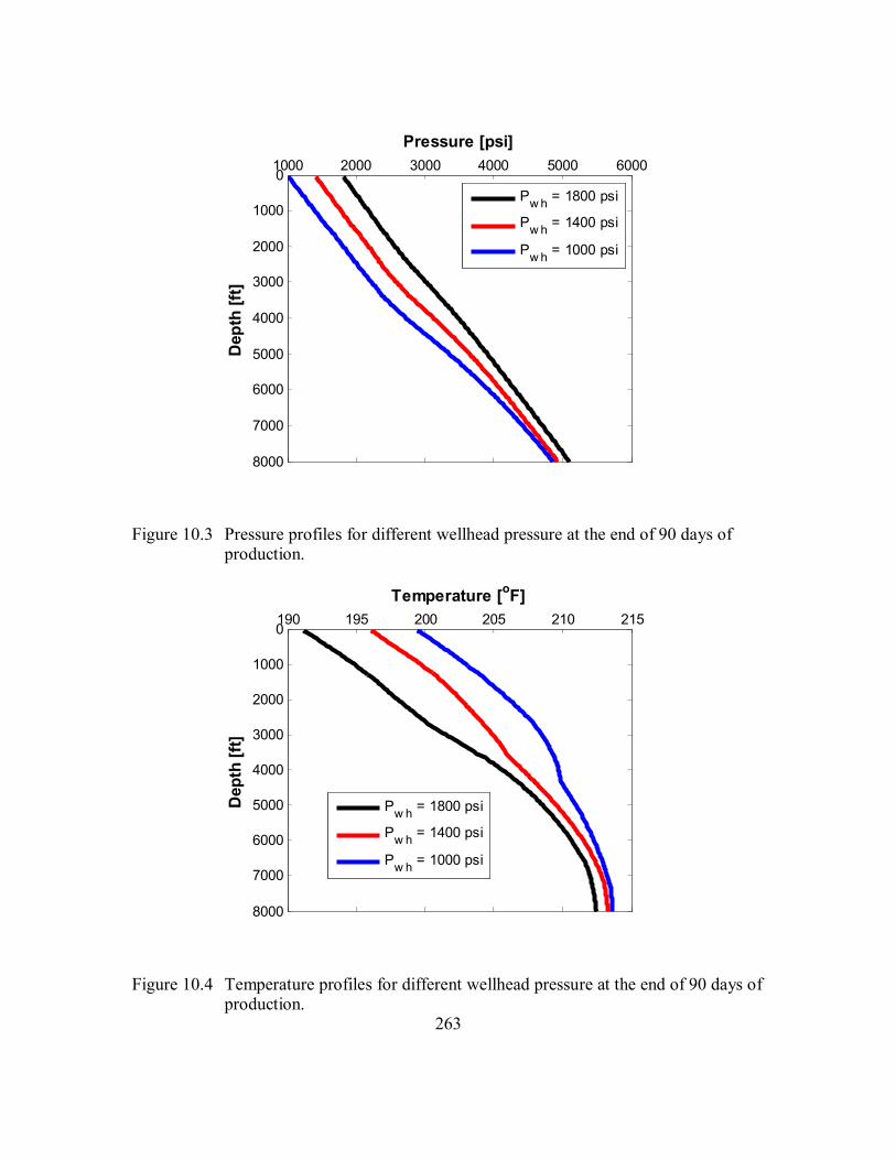
263
1000 2000 3000 4000 5000 60000
1000
2000
3000
4000
5000
6000
7000
8000
Dep
th [f
t]
Pressure [psi]
Pw h = 1800 psi
Pw h = 1400 psi
Pw h = 1000 psi
Figure 10.3 Pressure profiles for different wellhead pressure at the end of 90 days of production.
190 195 200 205 210 2150
1000
2000
3000
4000
5000
6000
7000
8000
Dep
th [f
t]
Temperature [oF]
Pw h = 1800 psi
Pw h = 1400 psi
Pw h = 1000 psi
Figure 10.4 Temperature profiles for different wellhead pressure at the end of 90 days of production.

264
0 0.01 0.02 0.03 0.04 0.050
1000
2000
3000
4000
5000
6000
7000
8000
Dep
th [f
t]
Asphaltene Thickness [ft]
Rti = 1.37 inRti = 1.62 inRti = 1.87 in
Figure 10.5 Asphaltene deposition thickness profiles for different tubing sizes at the
end of 90 days of production.
1000 2000 3000 4000 5000 60000
1000
2000
3000
4000
5000
6000
7000
8000
Dep
th [f
t]
Pressure [psi]
Rti = 1.37 inRti = 1.62 inRti = 1.87 in
Figure 10.6 Pressure profiles for different tubing sizes at the end of 90 days of production.

265
190 195 200 205 210 2150
1000
2000
3000
4000
5000
6000
7000
8000
Dep
th [f
t]
Temperature [oF]
Rti = 1.37 inRti = 1.62 inRti = 1.87 in
Figure 10.7 Temperature profiles for different tubing sizes at the end of 90 days of production.
0 0.2 0.4 0.6 0.8 1 1.2 1.40
1000
2000
3000
4000
5000
6000
7000
8000
Casph [10-3 lbmol/ft3]
Dep
th [f
t]
Rti = 1.37 inRti = 1.62 inRti = 1.87 in
Figure 10.8 Asphaltene flocculate concentration profiles for different tubing sizes at the end of 90 days of production.

266
0 2 4 6 8 10 12 140
1000
2000
3000
4000
5000
6000
7000
8000
Dep
th [f
t]
Oil Superficial Velocity [ft/sec]
Rti = 1.37 inRti = 1.62 inRti = 1.87 in
Figure 10.9 Oil superficial velocity profiles for different tubing sizes at the end of 90 days of production.
0 0.02 0.04 0.06 0.08 0.10
1000
2000
3000
4000
5000
6000
7000
8000
Dep
th [f
t]
Asphaltene Thickness [ft]
UTO = 1 Btu/ft2.hr.oF
UTO = 2 Btu/ft2.hr.oF
UTO = 3 Btu/ft2.hr.oF
Figure 10.10 Asphaltene thickness profiles for different overall heat transfer coefficient at the end of 90 days of production.

267
Chapter 11: Summary, Conclusions and Recommendations
This chapter presents the summary and the conclusions of this research and gives
recommendations for further extensions of this work.
11.1 SUMMARY
In the following, we summarize the work presented in this study.
Different modeling approaches for transient and steady state multiphase flow
calculation in the wellbore were presented in detail.
All the formulations for the conservation equations were derived. Constitutive relations
for interphase interaction and fluid/wall friction, plus flow regimes transition were
discussed and reproduced.
Drag force and interphase momentum transfer models were implemented in the
momentum equations to mimic the effect of different flow regimes.
Numerical stability and hyperbolicity of different multiphase flow models, such as
homogenous, drift-flux, and two-fluid for momentum equations, were discussed in
detail.
Eigenvalue analysis was performed for different multiphase flow models and the
regularization methods were applied in two-fluid models.
Fluid properties were calculated using EOS compositional model or blackoil model.
Mass transfer between phases was considered by either blackoil models or EOS
compositional models.
Wellbore heat-transfer model was presented with consideration of accurate analytical
and numerical models for surrounding materials temperature calculation.

268
The energy equation was solved numerically based on the enthalpy calculation.
Wellbore model solutions with consideration of semi-implicit, nearly-implicit, and
fully implicit methods were derived.
Final wellbore model solution was calculated for pressure, oil, water, and gas volume
fractions, temperature and water, oil and gas velocities.
Wellbore model solutions for different modeling approaches were compared against
each other for similar case studies. Computation time and accuracy of results were
evaluated for various models and numerical schemes.
The wellbore model was validated against analytical solutions and commercial
multiphase flow simulators. Model results were successfully compared against other
commercial simulators.
Thermodynamic modules were developed for wax and asphaltene precipitation based
on cubic EOS.
Phase behavior modules for asphaltene and wax were compared against experimental
data and a commercial phase behavior simulator (Winprop, CMG, 2008).
A chemical reaction package (PHREEQC) was coupled to the wellbore model for
simulating geochemical scales reaction and transportation in the wellbore.
Application of different particle fouling models for asphaltene and scale deposition
were discussed.
The deposition models for scale and asphaltene were derived for turbulent and laminar
flow regimes. For scale and asphaltene particles, two different approaches, the classical
stopping distance treatment and the stochastic modeling were described. Consistency
of derivations of the models was compared against two sets of experiments.
Wax deposition model was regenerated from available models in the literature.
Particle transportation and depositions were extended to multiphase flow systems.

269
Model results for asphaltene deposition during primary production and CO2 enhanced
oil recovery were presented and compared.
Different types of wellbore-reservoir coupling were discussed and an explicit coupling
was implemented.
A coupled horizontal and vertical wellbore model was also developed in which the
boundary condition could be assigned in the wellhead or bottom-hole.
An Equation-of-State compositional reservoir simulators (UTCOMP) were used for the
coupling purpose.
Asphaltene deposition in wellbore and in reservoir during the primary production
scenario was studied using a coupled wellbore/reservoir simulator.
Finally, the remediation procedure for asphaltene deposits removal was discussed
briefly. The developed wellbore model was also used for remediation and prevention
procedures with manipulation of the well operation conditions.
11.2 CONCLUSIONS
The conclusions from this study can be listed as follows:
For accurate and more realistic modeling of multiphase flow problems, two-fluid
model is the best choice. It is the most suitable approach for the co-current and
counter-current flows. Two-fluid models can consider the physics correctly. However,
this model is computationally more expensive. For this reason, the drift-flux models
with tuning for the slippage ratio can also be used for multiphase flow simulations in
the wellbore. Nevertheless, the drift-flux models are mostly appropriate for the
dispersed flows.

270
Regularization approaches are essential for two-fluid models to avoid stability issues in
numerical solutions. Additionally, discretization algorithms are crucial for the
computation time and the robustness of two-fluid models.
Modeling the phase behavior and the equilibrium condition of the hydrocarbon fluids is
the most important part of simulation of flow assurance issue in the wellbore. Correct
phase envelope calculation for the hydrocarbon fluids can qualitatively describe
whether or not the flow assurance problems can occur. In our phase behavior module,
we used cubic EOS. Using cubic EOS, we need proper tuning and fluid
characterization procedures to be able to capture the precipitation of asphaltene and
wax.
In addition to solid particles concentration in the flow, the transportation of the
particles in radial direction controls the particles deposition rate. Transportation of
particles in radial direction is a function of different parameters, such as particles size,
velocity field, temperature, and viscosity of the continuous fluid. More importantly, the
radial transportation is a function of flow regimes (turbulent or laminar). Flow regimes
can affect the mechanisms of depositions significantly. For instance, eddy currents
exist in the turbulent flow which can enhance particle diffusion in the transverse
direction. However, in the laminar flow, the momentum on the particles is only
transferred via viscose forces.
We achieved fairly good agreement for conditions at which the deposition models are
valid. In addition, our comparison shows that the described models in Chapter 7 are
applicable to asphaltene deposition in oil flow streams as well as particles deposition in
gas flow streams.
We observed that increasing the flow velocity and decreasing the tubing surface
temperature decreases the deposition rate significantly. From this observation, we

271
conclude that in the wellbore system, where velocity increases due to expansion and
temperature decreases due to thermal gradient from bottom-hole to the surface, the
deposition rate decreases remarkably.
Combination of transport coefficient in the radial direction and concentration of the
solid particles calculated from thermodynamic models determine the deposition rate in
the flow line. In any point in the wellbore where the combination of these two
parameters is maximum, the deposition rate is maximum. Consequently, the wellbore
cross-sectional area becomes a minimum at this point.
Our simulation studies reveal that the maximum deposition rate of asphaltene occurs in
a depth where pressure is close to the bubble point pressure. In addition, above that
depth, since light hydrocarbons flash out from crude oil, asphaltene becomes stable and
dissolves in the oil. For this reason, we observe a bell shaped profile for asphaltene
deposition in the wellbore.
Asphaltene deposition rate is not only a function of temperature and pressure, but also
of crude oil composition. Our results show that existence of light components like CO2
can significantly increase asphaltene problem in the wellbore. CO2 destabilizes
asphaltene in the phase envelope and increases both the bubble point pressure and the
asphaltene onset pressure. For this reason, when CO2 is mixed with an asphaltic crude
oil, it lowers the deposition sites in the wellbore to bottom-hole where the pressure is
larger. Our wellbore model can quantitatively determine how CO2 can change the
deposition of asphaltene in the wellbore.
Our simulation studies show that geochemical scales deposition mostly occurs in the
bottom of the well where the shear forces are low and particles can stick on the surface
of the well more easily.

272
Simulation of wax deposition shows that these components are very sensitive to
temperature. Since wax deposition occurs at very low temperatures, we mostly expect
to have this problem in the wellhead or in offshore pipelines that have significantly
lower temperature than the reservoir temperature.
For modeling flow assurance problems in the reservoir simulators, a coupled
wellbore/reservoir model is necessary. Our simulation results show that the asphaltene
deposition problem is more significant in the wellbore than in the reservoir. The
damage of asphaltene occurs in the reservoir when pressure goes below the onset
pressure. The precipitated asphaltene in the reservoir can flocculate to the wellbore and
cause more problems in the bottom of the well.
The coupled wellbore/reservoir simulator is capable of modeling multiple-zone
production from horizontal and vertical wells.
Finally we discussed remediation procedures for asphaltene problems in the wellbore.
Our simulation analyses show that manipulation of pressure and temperature can be a
possible method to reduce the asphaltene deposition problem. Operation condition of
the well can affect the thermodynamic equilibrium of asphaltene, as well as dynamic
transportation of these particles. We observed that decreasing the wellhead pressure to
below bubble-point pressure causes the asphaltene deposition interval to shrink and be
pushed to a lower part of the well.
11.3 RECOMMENDATIONS
The recommendations for further study in this area are presented in the following:
Since asphaltene components in the crude oil are the most polar components, they exert
molecular forces in their polar sites. This distinction of asphaltene components makes
the phase behavior of crude oil more complicated. In this study, we used compositional

273
flash calculation with cubic Equation-of-State to predict asphaltene precipitation at
different pressures and temperatures. Although this approach is more reliable than most
other solubility models for asphaltene, it lacks the consideration of correct molecular
interactions. In the Peng-Robnison Equation-of-State, in order to incorporate the effect
of molecular interactions in non-ideal solutions, binary interactions are used. Tuning
binary interaction coefficients may not be a mechanistic approach for asphaltene phase
behavior prediction, especially in cases where the crude oil composition is changed.
Recent developments in SAFT Equation-of-States have shown promising results in
modeling the phase equilibrium of systems containing heavy hydrocarbons such as
asphaltene (Gonzalez et al., 2005; Gonzalez et al., 2007). Since this Equation-of States
considers the interaction of the molecules correctly, this has better prediction capacity
for asphaltene precipitation. As a future work, we recommend implementation of
SAFT EOS for modeling asphaltene precipitation in the wellbore. Since UTWELL has
been developed in a way that can use different phase behavior models and Equations-
of-State for fluid property calculations, implementation of SAFT EOS in wellbore
calculations will be a simple task.
Particles deposition rate not only depends on the concentration but also on the speed of
particles traveling in the radial direction. The later term in the deposition models has
significant effect on the profile of deposits on the surface of the wellbore. In this
dissertation, we presented two types of deposition models for turbulent and laminar
flows. In those models, we used the classical analogy between mass transfer and
momentum transfer in radial direction for one-dimensional flow. Although the
deposition models that we applied in our wellbore calculation were validated against
experimental data, more validation for different flow situation is still owed. In addition,

274
for the sticking probability and attachment process of the solid particle, we used
simplified models which can be further improved and elaborated in the future.
In our wellbore model, we assume solid particles are small enough that can move with
the same speed of fluids in axial direction. In fact, we did not include the slip ratio of
fluid and solid particles in our calculations. Although our assumption is valid for light
and small particles, it is not appropriate for large particles. For this reason, we
recommend development of a similar liquid/gas drift-flux model for solid particles and
liquid drift velocity. Having this model, the convection terms of the mass conservation
equation for solid particle would be modified based on solid particle velocities.
The model we developed for geochemical scale deposition was only applied for the
standalone wellbore model. However, we know that the source of geochemical scales
is mostly the reactions that occur in the reservoir and the near wellbore region where
incompatible ions are mixed. In this scenario, a coupled wellbore/reservoir model is
needed to fully address the geochemical scales formation and transportation. For this
purpose, the development of geochemical reactions in the reservoir is necessary for
calculating the flocculated scales into the wellbore. This task requires coupling of
geochemical reaction module (PHREEQC) with transportation of solid particles in the
reservoir simulator.
To study the effect of light components in the crude oil for asphaltene deposition
mechanisms, we used our standalone wellbore model. Dynamic simulation of CO2
from the reservoir to the wellbore gives better insight of the effect of CO2 on
asphaltene deposition. A series of simulations are recommended to be performed using
the coupled wellbore/reservoir simulator to observe the effect of injected CO2 on
asphaltene formation in the reservoir and wellbore. Since CO2 flooding can be

275
combined with water injection, studying Water Alternative Gas injection is also
proposed for completeness of our simulation.
One of the remediation methods that were discussed in Chapter 10 is solvent
circulation. Aromatic agents or deasphalted oils are the main solvents that can be
circulated through injection annulus in the production wells to remove asphaltene
blockage from the surface of the wellbore. This process can be modeled combining the
thermodynamic modeling of solvent phase behavior with crude oil and the coupled
annulus / tubing fluid flow models. We recommend as a future work to develop an
annulus flow path for solvent injection to the wellbore. In this model, the effect of
temperature should be carefully modeled in the tubing and the annulus. Developing
annulus flow model can also be applied for other purposes such as gas-lift process
modeling in future.
There are some circumstances where asphaltene, geochemical scale, and wax
formations are combined in the flow line. These aspects might occur at the same time
in the mixing junctions of surface facilities or pipelines. In the current version of our
code, we only consider each flow assurance issue (asphaltene, wax, and scale)
separately. We also recommend combining these three flow assurance modules
together for such complicated scenarios.
The trajectory of our wellbore model is only a flow line with different angles. In the
current version of our code, we do not handle multiple junctions in the wellbore. We
recommend further development of UTWELL to implement the branches and junctions
for the application of multilateral wells, surface gathering systems, and platforms.
Developing this option can provide a complete surface facility network for the realistic
modeling of reservoir simulators.

276
Finally, we recommend developing analytical solutions for flow rate decline curves
and pressure transient models during asphaltene deposition in the wellbore. These
models can be used as diagnostic tools for detecting flow assurance problems in the
wellbore without full simulation of the wellbore flow.
277
Appendix A : Reservoir Simulation Model (UTCOMP)
In our coupled wellbore-reservoir model, we use a compositional reservoir
simulator called UTCOMP. This simulator, developed at The University of Texas, is an
isothermal, three dimensional, equation-of-state (EOS) IMPES (implicit pressure and
explicit phase saturations and compositions) compositional reservoir simulator.
UTCOMP is used to simulate a variety of important enhanced oil recovery processes,
such as immiscible and miscible gas flooding.
The following are some of the main features currently available in UTCOMP (User’s
Manual, 2003):
Three-dimensional EOS IMPES compositional
Rigorous and simplified flash calculations (including three-phase flash-calculation
capability)
K-value method for phase-behavior calculations
Higher-order total variation diminishing (TVD) finite-difference method
Full physical-dispersion tensor
Variable-width cross-section option
Vertical or horizontal well capability
Tracer-flood capability
Polymer-flood capability
Dilute-surfactant option with both equilibrium and non-equilibrium mass transfer
Gas-foam-flood capability (Pc* model and table-look-up approach)
Black-oil model
Asphaltene precipitation model

278
CO2 sequestration in aquifers
A.1 RESERVOIR GOVERNING EQUATIONS
Multi-component, multiphase flow in porous media occurs as a transport of
chemical species in multiple homogeneous phases under the influence of four
predominant forces: viscous, gravity, capillary and dispersion forces. The conservation
equation for each species should hold at each point of the medium. The general mass
conservation equation for component i can be presented as the following equation:
. 0 1, 2, ...,
NiV V x P D S K x q i nj j ij j j j j ij ijb b i ct (A.1)
The above equation is written in terms of moles per unit time, in which Ni is the
number of moles for component i per bulk volume, and qi is the molar injection (positive)
or production (negative) rate for component i. The mobility for phase j is defined as
follows:
jrj
j
kk (A.2)
Physical dispersion is modeled using the full dispersion tensor as presented in
equation (A-3):
K K Kxx xy xz
K K K Kij yx yy yzK K Kzx zy zz ij
(A-3)

279
The elements of above tensor contain contributions from two sources of
molecular diffusion and mechanical dispersion.
A.1.1 Volume Constraint
The volume constraint states that the pore volume in each of the cells must be
filled completely by the total fluid volume. This allows us to write the following
equation:
01 1
nn pcN L v Vi j j p
i j, (A.4)
where Lj is a ratio of moles in phase j to the total number of moles in the mixture.
Equation (A.1) and (A.4) combined with phase equilibrium equations (Appendix B) are
solved at each time step for a set of independent variables to be mentioned later.
A.1.2 Pressure Equation
Because of the IMPES nature of the UTCOMP simulator, the gridblock pressures
need to be implicitly solved first. The pressure equation used in UTCOMP is derived on
the premise that the pore volume should be filled completely by the total fluid volume:
Vt (P, N) = Vp (P) (A.5)
where the fluid is assumed to be a function of pressure and total number of moles of each
component and the pore volume are related to pressure only.

280
Assuming that the formation is slightly compressible, differentiating both
volumes with respect to time, using the chain rule to expand both terms against their
independent variables, and then rearranging and substituting Equation (A.1) into the
resultant equations yields the final pressure equation:
2
10 .1 1
1.
1 1
1 1 + . .
1 1 1
nn pcV PtV c V V k x Pp f ti rj j ijbP t i jnn pc
V V k x P Db ti rj j ij c j ji j
nn npc cV V S K x V qti j j ij ti ib
i j i
(A.6)
The above equation is solved for pressure (P) at a given time t. For the rest of the
physical quantities, values at the previous time level are taken. Note that the computation
of the derivatives tVP
and tiV involves the solution of two different sets of linear systems
with the size equal to the number of hydrocarbon components and constructed on the
basis of the phase-equilibrium relationship.
A.1.3 Overall Computational Procedure of UTCOMP
The overall solution scheme of UTCOMP follows a two-step procedure, which is
determined by the nature of the governing equations and solution strategy:
Solve implicitly the pressure equation, Equation (A.6), that involves the variables
in the adjacent gridblocks for the pressures of all the gridblocks using explicit saturation-
and phase-composition-dependent terms; those terms are computed using the physical
properties at the previous time level.

281
Compute overall number of moles for each component in each of the gridblocks
using the component molar-balance Equation (A.1). The flash calculations are then
performed to determine the phase amounts and compositions.
It should be noted that a set of linear equations is formed in the first step because
pressure is the only unknown in Equation (A.6). This distinct feature results in the
formulation of UTCOMP being non-iterative over a time-step. The detailed solution
procedure over a time-step is given below:
Compute the derivatives and coefficients necessary for Equation (A.6).
Solve implicitly Equation (A.6) for pressure at each of the gridblocks.
Update gridblock porosity at the new pressure.
Compute overall number of moles of component in each of the gridblocks using
Equation (A.1) with the new pressure and porosity.
Determine the equilibrium phase compositions and molar amount in each of the
gridblocks from the flash calculations.
Evaluate the phase saturations using phase molar amounts and molar densities.
Compute all other physical properties and desired injection/production streams.
Check if further calculation is needed by applying user-provided termination criteria. If
continuation is permitted, go to step (1) for the next time-step; otherwise, terminate the
simulation.
A.2 WELL MODEL
Well models in UTCOMP relate fluid influx/outflux between wellbore and the
reservoir through perforation zone. In general, a functional relation between the well rates
and flowing bottom-hole pressures is required to couple both reservoir and wellbore
models. In our coupled wellbore/reservoir simulator, the well models are based on

282
Peaceman (1991) and Babu et al. (1991). In addition, wellbore can handle different basic
well conditions such as
Constant bottom-hole flowing pressure injector
Constant molar rate injector
Constant volume rate injector
Constant bottom-hole flowing pressure producer
Constant molar rate production wells
Constant volume oil rate production wells
Constant wellhead pressure production wells
Generally, the relationship between volumetric flow rate, flowing bottom-hole
pressure, and gridblock pressure is expressed as
, Q PI P Pwf jj j (A.7)
where PI j is the phase productivity index for phase j . Chang (1990) showed that for a
one-dimensional case simulation the productivity index can be expressed as a function of
gridblock permeability and size as follows:
Δ
1, ,25.15ln
k k zx y rj
PI j nj prorw
(A.8)
This equation is valid for a well completed parallel to the z direction. The same
productivity index is defined for a well completed parallel to the y direction. In this
equation, permeabilities in the x and z directions (kx and kz) are used:

283
Δ 1, ,
25.15ln
k k yx z rjPI j nj pro
rw
(A.9)
where , z y are gridblock sizes (ft) in z and y directions, respectively. rj is the relative
mobility in 1cp . For rectangular well blocks in anisotropic reservoirs, an equivalent
radius is defined based on the well block dimensions. If the well is completed parallel to
the z axis (vertical well), then
1
11 222 2 2Δ Δ
0.28 1144
k ky xx yk kx y
rok ky xk kx y
(A.10)
Then, the same equation is used for a horizontal well parallel to the y axis
1
1 1 22 22 2Δ Δ
0.28 1 14 4
kk xz x zk kx z
rokk xz
k kx z
(A.11)
For equivalent radius equations, we assume that the grid spacing and permeability
in different directions are uniform (i.e., constant Δx, Δz, kx, and kz).

284
A.2.1 Constant Flowing Bottom-hole Pressure Injector
In this operation condition of the well, the flowing bottom-hole pressure for one
reference point is known. Well blocks pressure, component flow rates, and phase flow
rates at different perforation zones are calculated accordingly.
As a simplified assumption, considering pressure change with gravity only, the
perforation layer pressure becomes
( ),, P P z zwfz wf ref inj ref (A.12)
where ,Pwf ref is the known bottom-hole pressure at location zref . inj is the specific
gravity of the injected fluid at the well pressure. The injected fluid can have water phase
with fraction equal to 1f , and a hydrocarbon phase. Hydrocarbon component flow rates
in the perforation layers are calculated by
( ) [1 ] ( ) . 1, ...,1 q f z q i ni z i t z c (A.13)
For water phase also,
( ) ( ) ,1 1q f qnc z t z (A.14)
where ztq )( is the total flow rate into layer z
( )
( ) .( )
Qt zqt z vt inj
(A.15)
( )Qt z is the total volumetric flow rate into layer z

285
( ) ( ) [( ) ( ) ],1
npQ PI P Pj z wf z j zt z
j (A.16)
and
32( ) ( ) (1 ) ( ) ( ) ,
1 2 3
f LLv f inj injt inj (A.17)
where ( ) j inj is the molar density of phase j . 1j refers to the molar density of water,
2j is the molar density of oil and 3j is the molar density of gas phases. ( )L j inj is a
ratio of moles in hydrocarbon phase j to the total number of hydrocarbon moles in the
injection fluid.
A.2.2 Constant Molar Rate Injector
In this case, well constraint is the constant total molar rate tq . In contrast to
constant bottom-hole pressure scenario, for constant molar rate injectors first we
distribute the total molar flow rate into each layer, and then calculate pressure near the
perforated zones. We define molar flow rate for each hydrocarbon component as
1[1 ]( ) , 1,..., i i inj t cq f z q i n (A.18)
and for water phase as
1 1q f qnc t (A.19)

286
In multiple layer reservoirs, the total injection rates can be allocated to the
individual layers, according to a total mobility allocation scheme. This can be expressed
as the productivity index ratio. Hence,
( )( ) , 1,..., 1 ,...,
( )
b
f
i t zi z c f lz
t mm z
q PIq i n z z zPI
(A.20)
where zf and zl are the first and last layer numbers of a well, respectively. The total
productivity index of a layer z is defined as a summation of the productivity index for all
phases,
1( ) ( )
pn
jj
PI PIt z z (A.21)
where ( )zb
t mm zt
PI is the summation of the total productivity index over all
communicating layers for a well in a multi-layer reservoir. By knowing each layer molar
flow rate, it is possible to compute total volumetric flow rate as
3
1( ) ( ) ( ) ( ) ,
t z j z t z t inj
jQ Q q v (A.22)
where ( )t injv is defined as Equation (A.17).The bottom-hole pressure is then calculated
using the main definition of the productivity index
( )
( ) .( )
Qt zP Pwf z z PIt z
(A.23)

287
A.2.3 Constant Volume Rate Injector
The computational procedure for the constant volume rate injector well is similar
to that of a constant molar injection well. In this operation condition the gas injection rate,Qg (MSCF/D) and the water injection rate, Qw (STB/D) are given at standard
condition. In addition, the hydrocarbon composition of the injected fluid iz is specified.
First, we convert the known hydrocarbon volumetric rates to molar flow rates using the
following equation:
2.636 ( ) . 1,..., q Q z i ni g i inj c (A.24)
Similarly for water phase as
19.466 .1 q Qnc w (A.25)
Afterward, we follow the same procedure as described in Section A.2.2.
A.2.4 Constant Molar Rate Production Well
The total molar production rate, tq , is specified. The total production rate for each
layer is calculated using
1
1
( )( ) ,...,
( )
npt j j z
jt z f lnpzl
j j mm zf j
q PIq z z z
PI (A.26)

288
Again, we assume that the total production rates are allocated to the individual
layers according to a total mobility allocation scheme. Thus, at each layer, the component
rate can be calculated from
2( ) ( )
( ) , ,..., 1,...,( )
npt z j ij j z
ji z f l cnp
j j zj
q x PIq z z z i n
PI (A.27)
and for water phase from
1 1
1
1
( ) ( )( ) . ,...,( )
t z znc z f lnp
j j zj
q PIq z z zPI
(A.28)
Finally, the volumetric rates and molar rates are related by
1
( ) ( )( )( )
t z t zt z np
j j zj
q PIQPI
(A.29)
Calculating the volumetric flow production from each layer, the productivity
index definition can be used to obtain perforation layer pressure as
( )
( ) .( )
Qt zP Pwf z z PIt z
(A.30)

289
A.2.5 Constant Flowing Bottom-hole Pressure Producer
This operation condition of the well is similar to constant bottom-hole injection
well. Likewise, ignoring the friction pressure and acceleration terms, pressure in
perforation layers can be obtained from Equation (A.12). Additionally, the layer
component flow rate is calculated by
2( ) ( ) ( ) ,..., 1,...,
npi z j ij j z wf j z f l c
jq x PI P P z z z i n (A.31)
and
1 1 1 1( ) ( ) ( ) ,..., nc z z wf z f lq PI P P z z z (A.32)
A.2.6 Constant Volume Oil Rate Producer
In this case, the oil rate production, Qo is specified in standard condition. A flash
calculation is performed at separator conditions to determine the molar fraction of oil
phase in the produced hydrocarbon fluid using the overall hydrocarbon composition
computed from
2
2
( )( ) . 1,...,
( )
npzbj ij j m
m zt ji prod cnpzb
j j mm zt j
x PIz i n
PI (A.33)
The total molar flow rate is then calculated using

290
1
2
( )5.61
( ) ( ) ( )
npzbj j m
m zt jot npzb
o prod o prodj j m
m zt j
PIQq
L v PI (A.34)
The same allocation scheme for constant molar rate production wells is used to
compute the layer component rates. The same procedure discussed in section A.2.4 is
used to obtain the perforation layer pressure.
A.2.7 Constant Wellhead Pressure Producer/Injector
This boundary condition is common for the wells. However, this option in
UTCOMP is only available with the wellbore model. In fact, in this approach, well
blocks pressures are calculated from wellbore module, and then using similar approach to
Section A.2.1 or Section A.2.5 for injector or producer wells, well/reservoir influx or
outflux is calculated.
Using wellbore module, all the operation conditions at the wellhead, such as
constant flow rates or constant pressures, can be interpreted as constant bottom-hole
pressure condition. In fact, wellbore model can calculate the bottom-hole pressure for any
specified boundary condition and pass it to the reservoir simulator as constant bottom-
hole pressure for the source/sink calculation.

291
Appendix B: Compositional PVT Models
B.1 COMPRESSIBILITY FACTOR
A cubic EOS model is used to calculate pressure, temperature, and volume
relation of compositional PVT model as follows:
,2 2(1 )
RT apV b V Vb c cb
(B.1)
or,
,( )( )1 2
RT apV b V b V b
(B.2)
where 22 (1 )- (1 ) 4 ,1 c c c (B.3)
and 1 2 c . (B.4)
Using c = 1, Equation (B.2) becomes the Peng-Robinson Equation-of-State and
using c = 0, it becomes the Soave-Redlich-Kwong Equation-of-State.
The Peng-Robinson Equation-of-State (Peng and Robinson, 1976) is given as
follows:
( )- .
- ( ) ( - )
RT a TPV b V V b b V b
(B.5)
The parameters, a and b , for a pure component are computed from
2 2
( ) 0.45724 ( )R Tca T T
Pc (B.6)

292
0.07780RTcbPc
(B.7)
1 1
TTc
(B.8)
20.37464 1.54226 0.26992 0.49 if (B.9)
2 3 0.379640 + 1.485030 - 0.164423 + 0.016666 0.49 if (B.10)
For a multi-component mixture, a and b are obtained by mixing rules as follows:
(1 ),1 1
n nc ca x x a a ki j i j ij
i j (B.11)
,1
Ncb x bi i
i (B.12)
where ia and ib are for pure components. The constant ijk is the binary interaction
coefficient between components i and .j
Considering that PVZRT
, the Peng-Robinson Equation-of-State can be written in
the form:
3 2 0. Z Z Z (B.13)
In Equation (B.13), , , and are calculated as
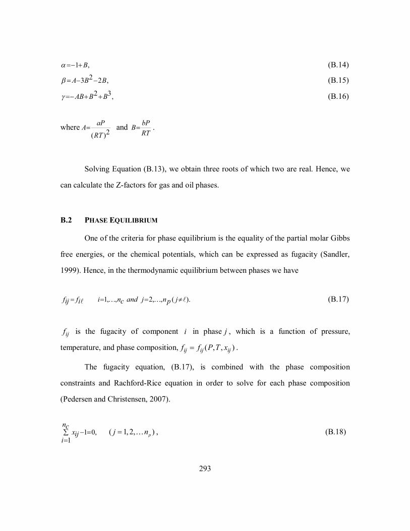
293
1 , B (B.14) 23 2 , A B B (B.15)
2 3, AB B B (B.16)
where 2( )
aPART
and bPBRT
.
Solving Equation (B.13), we obtain three roots of which two are real. Hence, we
can calculate the Z-factors for gas and oil phases.
B.2 PHASE EQUILIBRIUM
One of the criteria for phase equilibrium is the equality of the partial molar Gibbs
free energies, or the chemical potentials, which can be expressed as fugacity (Sandler,
1999). Hence, in the thermodynamic equilibrium between phases we have
1, , 2, , ( ). f f i n and j n jij i c p (B.17)
ijf is the fugacity of component i in phase j , which is a function of pressure,
temperature, and phase composition, ( , , )ij ij ijf f P T x .
The fugacity equation, (B.17), is combined with the phase composition
constraints and Rachford-Rice equation in order to solve for each phase composition
(Pedersen and Christensen, 2007).
1 0,1
ncxij
i ( 1, 2, )pj n , (B.18)

294
( 1) 0.1 ( 1)1
nc z Ki iv Kii
(B.19)
Phase composition is used for density and other properties calculation of the
phases.
B.3 DENSITY
After calculating the gas compressibility factor, the gas density 3( )lbmft
can be
obtained as follows:
. MW Pg
g Z RTg (B.20)
where, MWg is the gas molecular weight in ( )lbm
lbmol, P is pressure in ( )psi , R the
universal gas constant ,10.73, and T is the temperature ( )oR .
Oil density is also obtained from compositional flash calculation. In fact, at a
given temperature, pressure, and overall composition, oil phase Z-factor, oil molar weight
are calculated and used in Equation (B.21) to obtain oil density.
. MW Poo Z RTo
(B.21)
In Equation (B.21), MWo is the oil molecular weight in ( )lbmlbmol
, P is pressure
in ( )psi , R is universal gas constant 10.73, and T is temperature in ( )oR .

295
The dissolved gas-oil ratio ( )sR and the oil formation volume factor ( )oB are also
obtained by performing flash calculation at standard conditions
( 14.7 ,P psi 520 oT R ) and calculating the amount of oil and gas volume change
from a given condition to standard condition.
B.4 VISCOSITY
Lohrenz et al. (1964) presented different correlations for compositional oil and
gas viscosities calculation. Following are the equations.
* 0.000205 0.18
4 1* 0.18410
rr
r
(B.22)
where
( )1
ncx V ir i c
i (B.23)
2 3 41.023 0.2336 0.58533 0.40758 0.09332 , r r r r (B.24)
16
5.441 ,1 22 3
1 1
ncx Ti ci
i
n nc cx WM x Pi i i ci
i i
(B.25)

296
* 1 .
1
nc
x MWi i ii
ncx MWi i
i
(B.26)
The low-pressure pure component viscosity is calculated as follows:
5/80.0001776(4.58 1.67) ,
Trii
i (B.27)
where
1/65.44 .1/2 2/3 Tcii
MW Pi ci (B.28)
B.5 ENTHALPY
In the compositional calculation, the enthalpy is obtained from the excess
enthalpy ( Eh ) as follows:
( / )* 2ln( ).
2 1 1
v bT a T aEh h h pv RTv b
(B.29)
where, h is the system enthalpy and *h is the enthalpy at the ideal gas state. *h is
calculated from
* *, h x hi i
i (B.30)
where, * 2 3 4 5. h H H T H T H T H T H Ti A B C D E F (B.31)

297
In Equation (B.31), *ih is only a function of temperature ( )oR and cannot be
derived from an Equation-of-State. Passut and Danner (1972) have compiled the values
of AH through FH for components commonly encountered in petroleum engineering. In
most practical applications, the important variables are the enthalpy differences and not
the absolute enthalpies. Thus, the reference point for H can be chosen, arbitrarily.
Equation (B.29) can also be written in other form as
*,
, ( 2 1)( 1) ,
2 2 ( 2 1),
am jT am j Z Bj jT Ln RT Z jb Z Bm j j jh h (B.32)
where ,
am jT
is
1
1, 2( ) ( )(1 ),2 1 1
n na c c a am j k ix x a a a aij kj i k i k ikT T Ti k (B.33)
Since in the energy equation the derivative of enthalpy respect to temperature is required
in the Jacobian matrix this term can also be calculated as
2
, , 2 2,( 2 1)2
2 2 ( 2 1) 2 2 ( ( 2 1) )( ( 2 1) ), ,
B Za j jm j am j Z BT j jT am jZ B T Th j jT TLnT b Z B b Z B Z Bm j j j m j j j j j
*[( 1) ] .
Z hjR Z Tj T T (B.34)

298
321, 2[ ( ) ( )2 41 1
n na c c a am j k ix x a a a aij kj i k i kT TT i k
1 2 21 2( ) ( 2 )](1 ),2 22
a a a ak i k ia a a ai k i k ikT TT T (B.35)
20.45748[1 (1 )],
R Ta Ci i TriT P TC ri i (B.36)
2 20.45748 [1 ],2 1.52
a RiT P TC ri i
(B.37)
To validate the enthalpy calculation, we have compared our results with
Computer Modeling Group software (CMG, WINPROP version 2008.10) for a fluid
mixture of 50% C1 and 50% NC10, at T = 100 oF. As can be observed in Figures (B.1)
and (B.2), there is a good agreement between our results and the CMG calculation.
B.6 INTERFACIAL TENSION
The general equation for calculating the interfacial tension is (Reid et al, 1977)
1/4 ( ), ar l gP (B.38)
where σ is the interfacial tension in dyne/cm between the liquid and gas phases. j is the
molar density in mol/cm3 of phase j and par is the parachor. For multi-component systems
Equation (B.38) becomes
1/4
1( ).
cnar i l i g
iP x y (B.39)

299
where ix and iy are the composition of competent i in liquid and gas phases.
For hydrocarbon systems parchor can be a user-defined value or can be calculated
as
iariP CN (B.40)
40 1240.3 12
i
i
CNCN
(B.41)
CN is the carbon number of the component i.
Table B.1 Fluid properties calculation for a mixture of 50% C1 and 50% NC10 at 100 oF and 1000 psi
Liquid z-factor oZ 0.437
Gas z-factor gZ 0.886
Oil mole fraction ( / )oV lbmol lbmol 0.280
Oil mole fraction at standard condition ( / )soV lbmol lbmol 0.301
Oil molecular weight ( / )oMW lbm lbmol 103.68
Gas molecular weight ( / )gMW lbm lbmol 16.13
Oil density 3( / )o lbm ft 39.51
Gas density 3( / )g lbm ft 3.01
Bubble point pressure ( )Pb psi 1915
Solution gas oil ratio ( / )sR scf stb 273.94
Oil viscosity ( )o cp 0.28
Gas viscosity ( )g cp 0.00127
Oil formation volume factor ( / )oB rbbl stb 1.12
Gas formation volume factor 3( / )gB ft scf 0.00140

300
-800
-600
-400
-200
0
200
400
600
800
0 200 400 600 800 1000 1200
Pressure(psia)
Ho(
Btu
/lbm
ol)
CMGOur Model
Figure B.1 Oil phase enthalpy calculation and comparison with CMG for the mixture
of 50% C1 and 50% NC10, at 100 oF
3900
4000
4100
4200
4300
4400
4500
4600
4700
0 200 400 600 800 1000 1200
Pressure(psia)
Hg(
Btu
/lbm
ol)
CMGOur Model
Figure B.2 Gas phase enthalpy calculation and comparison with CMG for the mixture of 50% C1 and 50% NC10, at 100 oF

301
Appendix C: Black Oil PVT Models
C.1 GAS COMPRESSIBILITY FACTOR
For gas Z-factor calculation, there are different correlations in the literature.
Dranchuk and Abou-Kassem (1975) introduced the expression
23 5 7 82 41 1 63 4 5 2
A A A AA AZ A Ar rT T T T T Tr r r r r r
25 2 27 8 -A 1 exp( )9 10 11 112 3
A A rA A Ar r rT T Tr r r
. (C.1)
where
0.27 , Pr
r ZTr (C.2)
,TTr Tc
(C.3)
,PPr Pc
(C.4)
2187.0 330 71.5 , g gTc (C.5) 2706.0 51.7 11.15 , g gPc (C.6)
0.3265, -1.0700, -0.5339, 0.01569,-0.05165
A = .0.5475, -0.7361, 0.1844, 0.1056,0.6134,0.7210
Benedict et al. (1940) also introduced the expression (C.7) for gas compressibility
factor.

302
23 521 1 43
A AAZ A Ar rT T Tr r r
2
5 2 25 67 8 831 exp(- ),
rr r r
r r
A A A A AT T
(C.7)
where
0.31506237, -1.0467009, -0.57832729, -0.53530771,
A = .-0.61232032, -0.10488813, 0.68157001, 0.68446549
C.2 DENSITY
After calculating the gas compressibility factor, the gas density 3
lbmft
can be
obtained as follows:
, MW Pg
g Z RTg (C.8)
where gMW is the gas molecular weight in 3
lbmft
, P is pressure in ( )psi , R the universal
gas constant ,10.73, and T is the temperature ( )oR .
Oil density, by using the oil specific gravity ( )o , the oil formation volume
factor ( )oB , and dissolved solution gas-oil ratio ( )sR can also be calculated from blackoil
models. The Standing’s correlation (Standing, 1947) is used to estimate the dissolved
gas-oil ratio for saturated oils as follows:

303
1.204( ) ,18 10
PRs g yg (C.9)
where
g = Gas gravity (air =1)
gy = Gas mole fraction = 0.00091 0.0125T API
T = Reservoir temperature, oF.
For the saturated oil formation volume factor
bblBo stb, Standing (1947) presented
1.1750.972 0.000147 , B Fo (C.10)
where
( )0.5 1.25 .
gs
OSCF R T (C.11)
Using Equations (C.9) and (C.10), we can obtain the oil density as follows:
62.37 0.0136
,
Ro s g
o Bo (C.12)
where o is the oil gravity (for water equals to 1).
Other correlations have also been embedded in UTWELL for solution gas oil ratio
and oil formation volume factor. De Ghetto et al. (1994) and Vasquez and Beggs (1980)

304
correlations can also be selected for the solution gas oil ratio calculation. Vasquez and
Beggs (1980) correlation can also be used for the oil formation volume factor calculation.
C.3 VISCOSITY
For the blackoil model, there are two steps to calculate the oil viscosity. First, the
gas-free oil viscosity is obtained and then the gas-saturated oil viscosity is computed. For
the first step, Egbogah and Ng (1983) correlations can be applied:
( 1) 1.8653 0.025086 0.5644 ( ) log log log ToD API (C.13)
In Equation (C.13), oD , is the gas-free oil viscosity, at 14.7 psia. To calculate oil
viscosity, oD is used in the Beggs and Robinson (1975) correlation, such as
, BAo oD (C.14)
0.51510.715( 100) , A Rs (C.15) 0.3385.44( 150) . B Rs (C.16)
For the gas viscosity calculation, Lee et al. (1966) introduced the following
equations:
exp[ ], YK Xg g (C.17)
where

305
1.5(9.4 0.02 ),
209 19
MW TgKMW Tg
(C.18)
9863.5 0.01 , X MWgT (C.19)
2.4 0.2 . Y X (C.20)
In Equations (C.17) through (C.20), g is the gas viscosity ( )P , g is the gas
density ( )gcc
, gMW is the gas molecular weight and T is the temperature ( )oR . Other
correlations for viscosity of live oil, dead oil, and under-saturated oil from De Ghetto et
al. (1994) can be also used in UTWELL blackoil PVT.
C.4 ENTHALPY
The enthalpy is a function of pressure and temperature, via the heat capacity
( o
BtuC pFlbm
) and Joule-Thomson coefficient (
3
( )
F
Btuft
), as shown in Equation (C.21).
144( ) . dh C dT C dPj pj j j pjJc
(C.21)
Hence, enthalpy needs to be calculated with respect to a reference pressure and
temperature.
144( , ) ( , ) ( ) , T Ph T P h T P C dT C dPj j ref ref pj j pjT P Jref ref c
(C.22)
144( , ) ( ) . ref refT P
j pj j pjT Pc
h T P C dT C dPJ
(C.23)

306
In Equation (C.23) cJ is the conversion factor, j is the phase j Joule -
Thomson coefficient, and pjC is phase j heat capacity. The Joule-Thomson coefficient
can be calculated as follows:
1 1 1( ) .
Tj Cp Tj j jp (C.24)
The heat capacity can be calculated by different correlations for water, oil, and
gas. Holman (1958) has reported the following equation for specific heat capacity of
water for the range of 20 oC to 290 oC.
4245 1.841( / . ) .
TCp J kg Kw
w (C.25)
Gambill (1957) has presented the following equation to calculate the specific heat
capacity of oil as a function of temperature and oil-specific gravity:
1684 3.389( / . ) .
TCp J kg Kooil
(C.26)
Waples D.W and Waples J.S (2004) presented the temperature dependence of the
specific heat capacity for natural gas using a fourth-order polynomial:
4 3 2( / . ) . oCp Btu lbm F AT BT CT DT Eg (C.27)

307
The coefficients in Equation (C.27) are functions of pressure. For instance, the
following polynomials are used for methane:
22 3 18 2 16 13
19 3 15 2 12 10
16 3 12 2 11
( ) -2.52 10 1.34 10 -9.15 10 1.62 10
( ) 5.37 10 - 2.85 10 1.37 10 - 4.67 10
( ) -3.47 10 1.86 10 2.01 10 3.95 10
A P P P P
B P P P P
C P P P P
17
14 3 10 2 7 4
11 3 8 2 4 1
( ) 7.70 10 - 4.21 10 - 5.96 10 3.70 10
( ) -1.03 10 5.24 10 1.55 10 4.88 10 .
D P P P P
E P P P P
C.5 INTERFACIAL TENSION
For gas and oil interfacial tension the correlation by Baker and Swerdloff (1955)
37.7 0.05 100.0 0.26 T APIog
4 7 2 11 3 1.0 7.1 10 2.1 10 2.37 10 . P P P (C.28)
For gas and water the correlation by Katz (1955) is used
70.0 0.1 74.0 0.002 . T Pwg (C.29)
`

308
Appendix D: Derivation of Balance Equations
In many transport systems, field equations are derived to solve the motion of
fluids. These equations are usually described based on the conservation laws for mass,
momentum, energy, charge, etc. In addition, the constitutive relations and state relations
are combined with the conservation laws to explain the interaction and the property of
phases respectively.
In this appendix, we briefly discuss the derivation of field equations for single-
phase and multi-phase flow systems as shown in Chapters 3 and 4. We follow similar
approach discussed in Ishii and Hibiki (2011) for the derivation of these equations.
D.1 GENERAL BALANCE EQUATIONS IN SINGLE-PHASE FLOW
The conceptual models in single-phase flow systems are well-established in
continuum mechanics. Single-phase systems are homogenous media with defined
boundaries around the fluid.
We can derive the differential balance equation of single-single phase flow
system from general integral balance. Assuming a bulk of fluid with density of , Figure
D.1, the general integral balance for any quantity of becomes
. , m m mV A V
d dV n JdA dVdt
(D.1)
where mV is the material bulk volume, mA is the material surface area , J is the flux of
from the surface of material and is the body source of quantity . Equation (D.1)

309
explains that summation of body source change of quantity plus the integration of
mass flux through the surface boundary of the control volume, mV , is equal to the
accumulation of quantity in the bulk of fluid. Using the Leibnitz rule for the left hand
side integration of Equation (D.1), we obtain
. . .
m m m mV A A VdV u ndA n JdA dV
t (D.2)
Differentiating Equation (D.2) respect to dV , we obtain
. . .
u J
t (D.3)
Equation (D.3) is the differential balance equation for single-phase flow. This equation
can be converted to the mass, momentum and energy equations with proper definitions
for the quantity , the flux gradient, J , and the body source and sink terms, .
For example, assuming 1 , 0J , 0 , Equation (D.3) becomes mass
conservation equation as
. 0.
u
t (D.4)
Accordingly, introducing u (actual velocity), J T pI (pressure and viscous
stress tensor) and g (gravity acceleration), we obtain momentum conservation
equation as
. . .
u u P gt
(D.5)

310
Finally for 2
2
ue , . J q T u , .
qg u , we achieve the energy conservation
equation as
2
22. . . . . ,
2
ueue u q T u g u q
t (D.6)
where e is the internal energy, q is the heat flux, q body heat loss/gain.
D.2 GENERAL BALANCE EQUATIONS IN MULTIPHASE FLOW
In multiphase flow systems, a great deal of difficulties is encountered for
derivation of field equations due to discontinuity of the bulk of fluids. In contrast to
single-phase flow, multiphase flow systems are no longer homogeneous media and
consequently are not continuously differentiable in the integration region. In fact, the
presences of interface between fluids (such as bubble and liquid or droplet and gas) in a
bulk of fluids causes source of discontinuities. Thus, to derive the field equations in the
multiphase flow systems the continuity of flow parameters should be maintained by
averaging the bulk of fluids. For this reason, in multiphase flow systems understanding
the local characteristic of the flow and methods for up-scaling (averaging) the
microscopic phenomena between multiphase fluids are crucial.
Averaging procedures of parameters can be classified into three groups:
1) Eulerian Mean Value
Function: ( , )F F t x
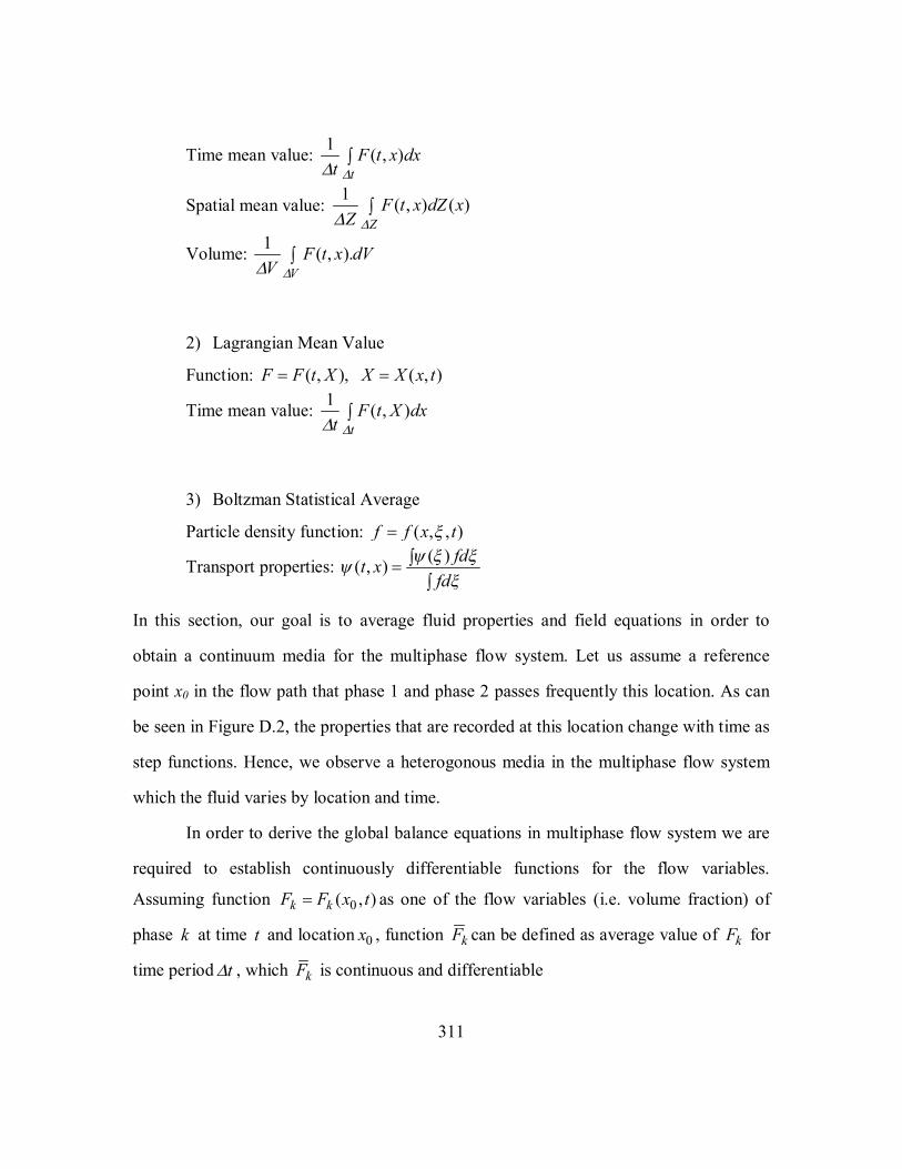
311
Time mean value: 1 ( , )tF t x dx
t
Spatial mean value: 1 ( , ) ( )Z
F t x dZ xZ
Volume: 1 ( , ).V
F t x dVV
2) Lagrangian Mean Value
Function: ( , ), ( , ) F F t X X X x t
Time mean value: 1 ( , )tF t X dx
t
3) Boltzman Statistical Average
Particle density function: ( , , )f f x t
Transport properties: ( )( , )
fdt xfd
In this section, our goal is to average fluid properties and field equations in order to
obtain a continuum media for the multiphase flow system. Let us assume a reference
point x0 in the flow path that phase 1 and phase 2 passes frequently this location. As can
be seen in Figure D.2, the properties that are recorded at this location change with time as
step functions. Hence, we observe a heterogonous media in the multiphase flow system
which the fluid varies by location and time.
In order to derive the global balance equations in multiphase flow system we are
required to establish continuously differentiable functions for the flow variables.
Assuming function 0( , )k kF F x t as one of the flow variables (i.e. volume fraction) of
phase k at time t and location 0x , function kF can be defined as average value of kF for
time periodt , which kF is continuous and differentiable

312
01 ( , ) .
k k
tF F x t dt
t (D.7)
In other word, our interpretation from kF is the probability of seeing phase k at
location 0x at neighborhood of time t . This definition actually scales the microscopic
phase dynamics phenomena to macroscopic scale with continuum attribution. Using
Equation D.7 for phase volume fraction we obtain
0 01( , ) ( , ) ,
k k
tx t M x t dt
t (D.8)
where 0( , )kM x t is one when phase k exist at location 0x and is zero when it does not
exist. Hence, 0( , )k x t means the probability of existence of phase k at location 0x .
0( , )k x t can also be defined as kM according to Equation D.7.
Using the following definitions, we can also obtain the volume and mass average
functions as
,
k k kk
kk
M F FFM
(D.9)
.
k k k k
k k
(D.10)
Using the definitions explained in Equations D.7 through D.10, Ishii and Hibiki
(2011) derived the general balance equation for multiphase flow system as follows:

313
. . ,
Tk k k
k k k k k k k k k k kX X u J J I
t (D.11)
where kX is weighted quantity mean value, ku weighted mean velocity of phase k , kJ
is surface flux of phase k , TkJ is turbulent flux, k is body source and kI is interfacial
source term.
Consequently, similar to the single-phase model, Equation D.11 can be converted to
mass, momentum and energy balance equations with appropriate definitions for the
quantity variables. Assuming 1kX , 0kJ , 0TkJ , 0 k and k kI (interphase
mass transfer rate), mass balance equation for phase k becomes
. .
k k
k k k kut
(D.12)
Like-wise for k kX u (actual velocity),
kk k kJ T P I (pressure and viscous shear
tensor), TT
kkJ (turbulent shear tensor), k kg (gravity acceleration), and
k kI M (interphase momentum transfer rate), momentum balance equation for phase
k becomes
. . . .
Tk k k kk k k k k k k k k k k ku u u P g M
t (D.13)
For energy balance equation we use 2
2 k
k kuX e (internal energy and kinetic
energy), . k k k kJ q T u (condition and friction heat flux), T Tk kJ q (turbulent heat flux),

314
.
k
k k kk
qg u (gravity potential and heat loss/gain) and k kI E (interfacial heat
transfer) to obtain
2 2.
2 2
. . . .
k kk k k k k k k
Tk k k k k k k k k k k
u ue e ut
q q T u g u E
(D.14)
Equations D.12 through D.14 are the differential balance equations for multiphase
flow systems that have been used in our multiphase flow calculations with some
simplifications.
D.3 BASIC ASSUMPTIONS
In Chapters 3 and 4, we added the following assumptions to the general balance
equations in Section D.1 and D.2 to obtain the final format of our conservation equations
for single-phase and multiphase flow models:
One-dimensional flow with Eulerian coordination is used.
Flow path can have arbitrary cross section (with defined hydraulic diameter) and
arbitrary trajectory in (x, y, z) coordination.
Field units are considered in the equations of Chapters 3 and 4. Conversion factors
such as cg and cJ are included in the equations.
Flow path can be surrounded by reservoir as a tank model. Hence the influx terms for
each phase from reservoir (k ) is added to the mass balance equations (Equation
D.12).

315
Deposition rate ( ,d sm ) for the solid phase is also considered in the mass balance
equation for solid phase.
Physical dispersion for mass transfer is neglected in the axial direction.
Phases are liquid (mixture of oil and water) and gas in the momentum equation.
Oil and water slippage in the liquid system is considered via drift-flux models.
Momentum interface models in Equation D.13 is replaced by RELAP5 (2011) one-dimensional models as M u u u FIKkk k ki k k i .
Shear tensor ( k ) and turbulent tensor (T
k ) momentum transfer terms in momentum
balance equations are neglected and one-dimensional wall-phase shear forces are
included using RELAP5 (2011) approach, u FWKk k k k .
Phase pressures are all assumed to be the same , 1, ..., . P P k nk
We use the summation of energy balance equations for each phase to obtain the
temperature in the fluids.
Enthalpy is used instead of internal energy in the energy equation.
Enthalpy influx terms for each phase from reservoir ( k ) is added to the total energy
balance equation.
Phase temperatures are all assumed to be the same , 1, ..., . T T k nk
Interfacial heat transfer is neglected.
Conduction heat transfer in axial direction ( . q ) in the energy equation is neglected.
Shear stress (friction) heat transfer term ( . . T u ) in the energy equation is neglected.
Turbulent heat flux in axial direction ( Tq ) in the energy equation is neglected.
Local equilibrium and negligible capillary pressure effect on hydrocarbon
thermodynamic equilibrium is considered in the system.
Up to four phases are allowed to exist in the model as water, oil, gas, and precipitated
solids.

316
Hydrocarbon mixture is assumed as nc components with no water.
The aqueous phase is pure water plus dissolved ions and solid precipitates.
The bubbles coalescence and break up is neglected.
Figure D.1 Fluid bulk control volume
Figure D.2 Density change with time at point x0
mV mA
t
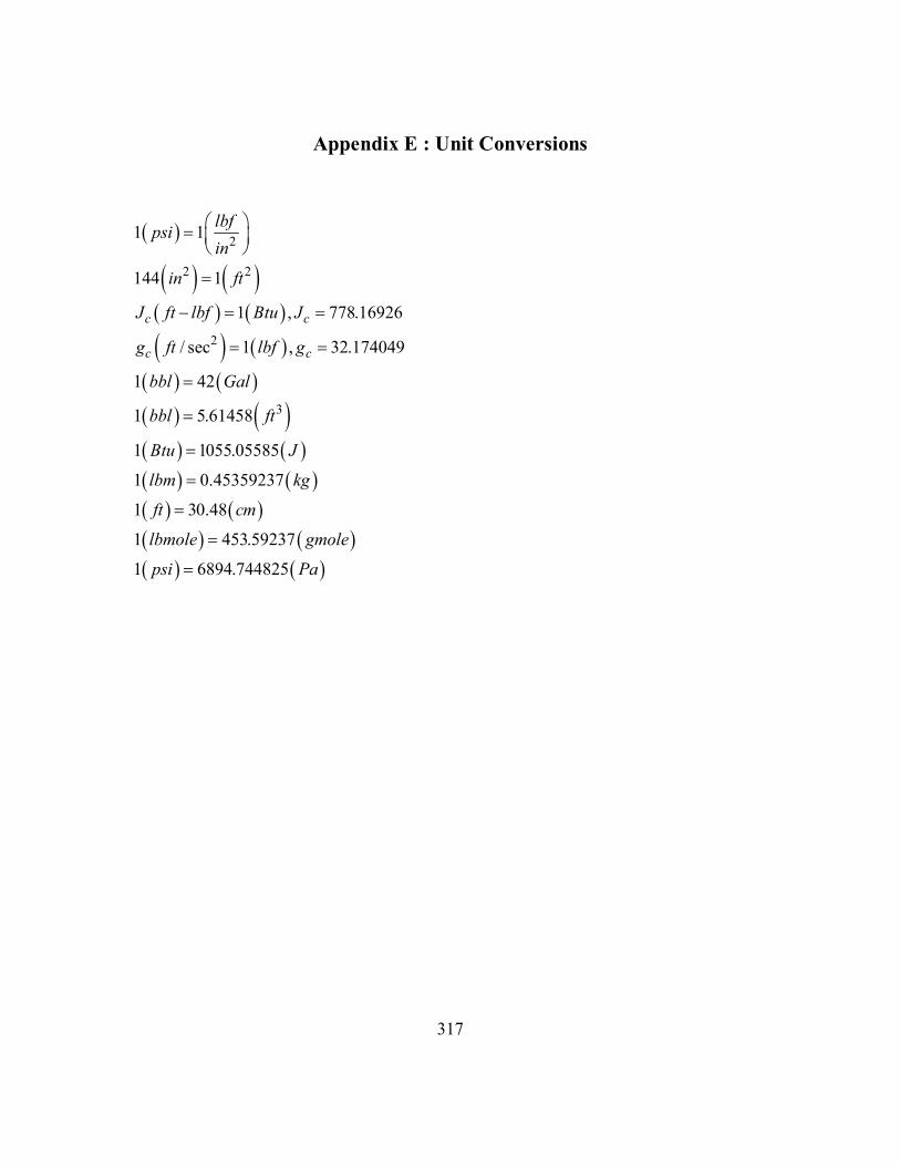
317
Appendix E : Unit Conversions
2
2 2
2
3
1 1
144 1
1 , 778.16926
/ sec 1 , 32.174049
1 42
1 5.61458
1 1055.05585
1 0.45359237
1 30.48
1 453.59237
1 6894.744825
c c
c c
lbfpsiin
in ft
J ft lbf Btu J
g ft lbf g
bbl Gal
bbl ft
Btu J
lbm kg
ft cm
lbmole gmole
psi Pa

318
Appendix F: UTWELL Keywords
The main UTWELL input file (INPUT.CFG) consists of comment lines (starting
with CC) and keyword lines (starting with *). The UTWELL simulator ignores all
comment lines.
If more than one well is introduced in the input data include files can be defined
and the wells input data can be stored in the include files separately.
Input variables are read in the following order: Well trajectory, casing data, tubing data and formation data Fluid properties Reservoir data Process condition Initial condition Boundary conditions Output options Numerical options
F.1 FLOW PATH DEFINITION AND TRAJECTORY F.1.1 NWLBR, FLOWPATH, INCLUDE NWLBR - Total number of wells/flow-paths in the simulation FLOWPATH - Type of flow paths Possible values: WELL PIPELINE INCLUDE - Name of the include files for each well F.1.2 LW, WNAME LW - Well index WNAME - Well/flow path name F.1.3 MAXGRIDSIZE, WSURFACE MAXGRIDSIZE - Maximum size of the wellbore gridblock, [ft]

319
WSURFACE – Wellbore surface datum, [ft] F.1.4 TRAJINTVL, MD, TVD, INCLINATION, AZIMUTH TRAJINTVL - Number of the trajectory intervals in the wellbore MD - Measured depth of well’s intervals, [ft] TVD - True vertical depth of well’s intervals, [ft] INCLINATION - Inclination of each interval of the well trajectory, [deg] AZIMUTH - Azimuth angle of each interval of the well trajectory, [deg]
F.1.5 CASEINTVL, HANGERDEPTH, SETTINGDEPTH, RCI, RCO, RWB CASEINTVL - Number of casing surrounding the well HANGERDEPTH - Hanger depth of each casing, [ft]
SETTINGDEPTH - Setting depth of each casing, [ft] RCI - Inner radius of each casing, [ft] RCO - Outer radius of each casing, [ft] RWB - Wellbore radius around each casing, [ft]
F.1.6 CEMENTOP, EPSCI, EPSCO, KCASE, KCEM, HCFC, CASEANLSFLUID CEMENTOP - Top elevation of the cement, [ft]
EPSCI - Inner emissivity of the casing, [ft] EPSCO - Outer emissivity of the casing KCASE - Casing heat transfer conductivity, [Btu/hr-ft-oF] KCEM, Cement heat transfer conductivity, [Btu/hr-ft-oF] HCFC, Tuning factor for the total heat transfer in the casing CASEANLSFLUID, Type of the fluid ID between annulus and casing, which is chosen from Annuls fluid database
F.1.7 OPENHOLE_LENGTH, OPENHOLE_RWB, OPENHOLE_ROUGHNESS
x (lw,1)
z
TVD (lw,1)
MD(lw,1)

320
OPENHOLE_LENGTH - Length of open hole perforation zone, [ft] OPENHOLE_RWB - Diameter of flow path in the open-hole zone, [ft] OPENHOLE_ROUGHNESS - Flow path roughness in the perforation zone, [ft/ft]
F.1.8 TUBINTVL, TUBETOP, TUBEBOTT, RTI, RTO TUBINTVL - Number of tubing intervals in the well trajectory TUBETOP - Top depth of tubing interval, [ft] TUBEBOTT - Bottom depth of tubing interval, [ft] RTI - Inner radius of tubing interval, [ft] RTO - Outer radius of tubing interval, [ft]
F.1.9 EPSTO, KTUB, CKNESS, KINS, HCFT, TUBANLSFLUID, ROUGHNESS
EPSTO - Outer emissivity of the tubing KTUB - Tubing heat transfer conductivity, [Btu/hr-ft-oF] INSTHICKNESS - Thickness of the insulator around the tubing, [ft] KINS - Insulator heat transfer conductivity, [Btu/hr-ft-oF] HCFT - Tuning factor for overall heat transfer factor of tubing TUBANLSFLUID - Type of the fluid between annulus and tubing ROUGHNESS - Surface roughness of the tubing, [ft/ft]
F.1.10 FORMINTVL, FORMATIONTOP, FORMATIONBOTT FORMINTVL - Number of different formation types
FORMATIONTOP - Top depth of the formation, [ft] FORMATIONBOTT - Bottom depth of formation type, [ft]
F.1.11 FORMATIONTVD, KEARTH, DENEARTH, CEARTH, TAMBTOP, TAMBOTT
FORMATIONTVD - True vertical depth of the formation, [ft] KEARTH - Surrounding formation heat transfer conductivity, [Btu/hr-ft-oF] DENEARTH - Surrounding formation density, [lbm/ft3] CEARTH - Surrounding formation heat capacity, [Btu/lb.oF] TAMBTOP - Ambient temperature at the surface of the interval, [oF] TAMBOTT - Ambient temperature at the bottom of the interval, [oF]
F.1.12 IUTO, UTOTAL
IUTO - Heat transfer coefficient flag Possible values
0: internal calculation 1: constant user specified value UTOTAL - Total heat transfer coefficient for IUTO = 1, [Btu/ft2-sec-oF]
F.2 FLUID PROPERTY
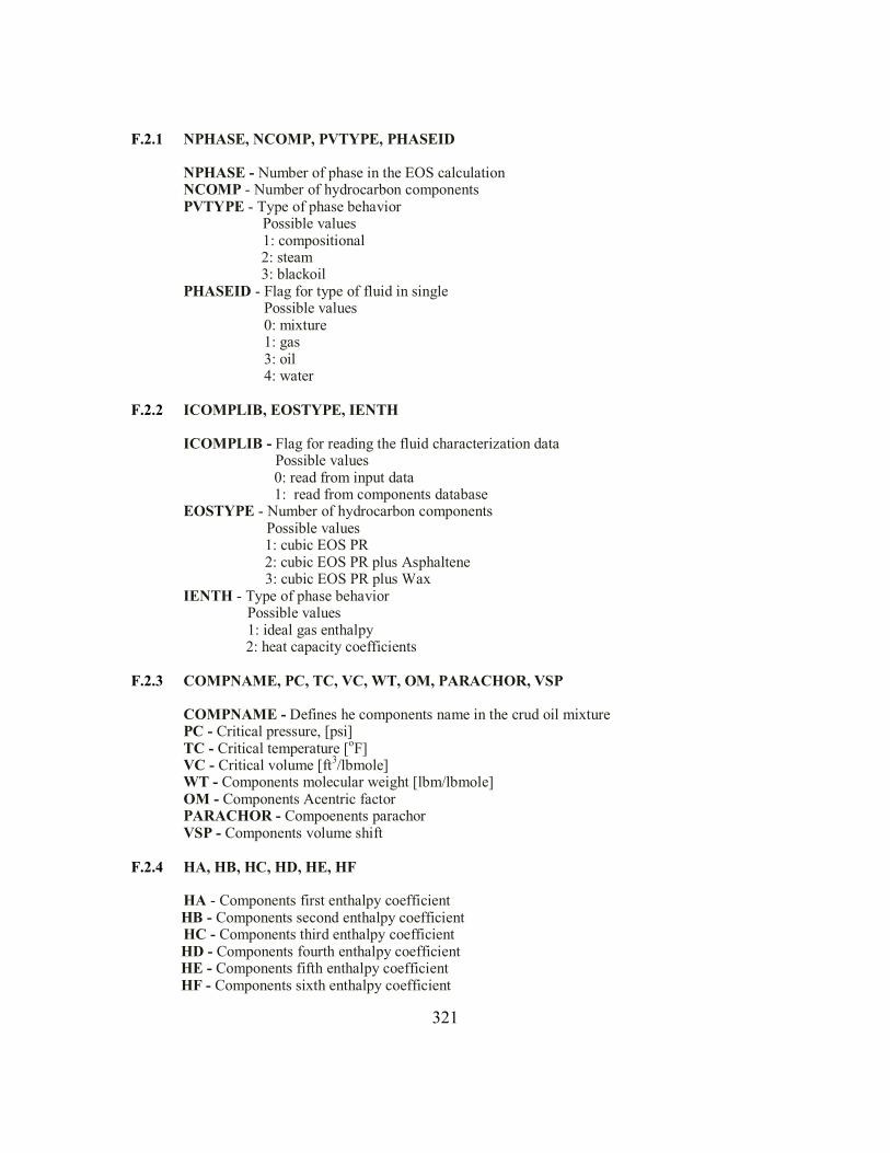
321
F.2.1 NPHASE, NCOMP, PVTYPE, PHASEID
NPHASE - Number of phase in the EOS calculation NCOMP - Number of hydrocarbon components PVTYPE - Type of phase behavior Possible values 1: compositional 2: steam 3: blackoil
PHASEID - Flag for type of fluid in single Possible values 0: mixture 1: gas 3: oil 4: water
F.2.2 ICOMPLIB, EOSTYPE, IENTH
ICOMPLIB - Flag for reading the fluid characterization data Possible values 0: read from input data 1: read from components database
EOSTYPE - Number of hydrocarbon components Possible values 1: cubic EOS PR 2: cubic EOS PR plus Asphaltene 3: cubic EOS PR plus Wax IENTH - Type of phase behavior Possible values 1: ideal gas enthalpy 2: heat capacity coefficients F.2.3 COMPNAME, PC, TC, VC, WT, OM, PARACHOR, VSP
COMPNAME - Defines he components name in the crud oil mixture PC - Critical pressure, [psi] TC - Critical temperature [oF] VC - Critical volume [ft3/lbmole] WT - Components molecular weight [lbm/lbmole] OM - Components Acentric factor PARACHOR - Compoenents parachor VSP - Components volume shift
F.2.4 HA, HB, HC, HD, HE, HF
HA - Components first enthalpy coefficient HB - Components second enthalpy coefficient HC - Components third enthalpy coefficient HD - Components fourth enthalpy coefficient HE - Components fifth enthalpy coefficient HF - Components sixth enthalpy coefficient

322
F.2.5 DELTA(IC, IC) DELTA(IC, IC) - Components binary interaction coefficients F.2.6 RSCORR, RSCALIBRATE, ZGCORR, DOVCORR, VISGCORR, IFTOGCORR,
IFTWGCORR, ETNHCORR RSCORR - Correlation flag for solution gas oil ratio Possible values 1: De Ghetto 2: Vazquez / Beggs RSCALIBRATE - Flag for calibration of the solution gas oil ratio Possible values 0: No scaling 1: Scaling ZGCORR - Correlation flag for the gas compressibility factor Possible values 1: Robinson 2: Yarborough / Hall 3: Dranchuck / Abu-Khassem DOVCORR - Correlation flag for dead oil viscosity Possible values 1: De Ghetto VISGCORR - Correlation flag for gas viscosity Possible values 1: Lee-Gonzalez –Eakin (1) 2: Lee-Gonzalez –Eakin (2) – PIPESIM 2011 IFTOGCORR - Correlation flag for gas and oil interfacial tension Possible values 1: Baker / Swerdloff IFTWGCORR - Correlation flag for water gas interfacial tension Possible values 1: Katz ENTHCORR - Correlation flag for enthalpy calculation Possible values 1: Default method 2: PIPESIM 1983 method (no Joule Thomson effect) 3: PIPESIM 2009 method (with Joule Thomson effect) F.2.7 PSEP, TSEP, PBUB, TBUB, RSBUB PSEP - Separator pressure [psi] TSEP - Separator temperature [oF] PBUB - Bubble point pressure [psi] TBUB - Bubble point temperature [oF] RSBUB - Solution gas oil ration at the bubble point pressure [ft3/bbl] F.2.8 CPW, CPO, CPG, CPWMETHOD, CPOMETHOD, CPGMETHOD, DHVAP
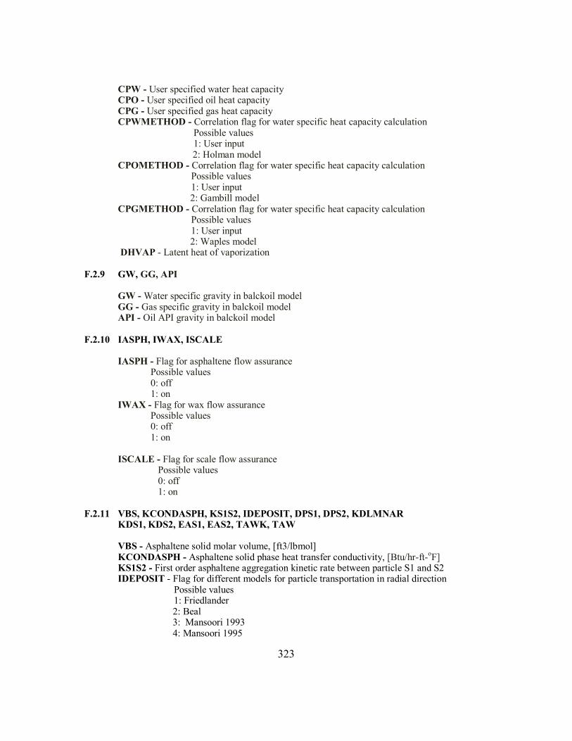
323
CPW - User specified water heat capacity CPO - User specified oil heat capacity CPG - User specified gas heat capacity CPWMETHOD - Correlation flag for water specific heat capacity calculation Possible values 1: User input 2: Holman model CPOMETHOD - Correlation flag for water specific heat capacity calculation Possible values 1: User input 2: Gambill model CPGMETHOD - Correlation flag for water specific heat capacity calculation Possible values 1: User input 2: Waples model DHVAP - Latent heat of vaporization F.2.9 GW, GG, API GW - Water specific gravity in balckoil model GG - Gas specific gravity in balckoil model API - Oil API gravity in balckoil model F.2.10 IASPH, IWAX, ISCALE IASPH - Flag for asphaltene flow assurance Possible values 0: off 1: on IWAX - Flag for wax flow assurance Possible values 0: off 1: on ISCALE - Flag for scale flow assurance Possible values 0: off 1: on F.2.11 VBS, KCONDASPH, KS1S2, IDEPOSIT, DPS1, DPS2, KDLMNAR KDS1, KDS2, EAS1, EAS2, TAWK, TAW VBS - Asphaltene solid molar volume, [ft3/lbmol]
KCONDASPH - Asphaltene solid phase heat transfer conductivity, [Btu/hr-ft-oF] KS1S2 - First order asphaltene aggregation kinetic rate between particle S1 and S2 IDEPOSIT - Flag for different models for particle transportation in radial direction Possible values 1: Friedlander 2: Beal 3: Mansoori 1993 4: Mansoori 1995

324
5: Clever and Yates DPS1 - Smallest asphaltene particle size, [cm] DPS2 - Largest asphaltene particles size, [cm] KDLMNAR - Transport coefficient tuning factor for laminar flow KDS1 - Transport coefficient tuning factor for turbulent flow for the smallest particles KDS2 - Transport coefficient tuning factor for turbulent flow for the largest particles EAS1 - Activation energy for smallest particles adhesion forces on the surface, [kJ] EAS2 - Activation energy for the largest particles adhesion forces on the surface, [kJ] TAWK - Shear force removal tuning factor TAWA - Shear force removal power coefficient TAWMAX – Maximum shear force for deposit removal, [psi] F.2.12 PORMAX, PORCB, PORCZ, TAWA, SURFCOEF, HLDPCOEF, KDWAX,
KCONDWAX PORMAX – Wax crystal maximum porosity PORCB – Wax porosity power coefficient PORCZ – Wax shear stress power coefficient for porosity reduction SURFCOEF – Wetted surface area power coefficient for wax multiphase flow deposition
rate HLDPCOEF - Holdup power coefficient for wax multiphase flow deposition rate KDWAX - Transport coefficient tuning factor for wax deposition KCONDWAX – Wax solid phase heat transfer conductivity, [Btu/hr-ft-oF] F.2.13 KCONDSCALE, IDEPOSITAQ, DPSAQ, KDLMNRAQ, KDAQ, EAQ KCONDSCALE - Scale solid phase heat transfer conductivity, [Btu/hr-ft-oF] IDEPOSITAQ - Flag for different models for scale transportation in radial direction Possible values 1: Friedlander 2: Beal 3: Mansoori 1993 4: Mansoori 1995 5: Clever and Yates DPSAQ - Scale particle size, [cm] KDLMNRAQ - Transport coefficient tuning factor for scale deposition in laminar flow KDAQ - Transport coefficient tuning factor for scale deposition in turbulent flow EAQ - Activation energy for scale adhesion forces on the surface, [kJ] F.2.14 NONSET, PSTAR, TSTAR NONSET - Number of aspahltene precipitation onset data PSTAR - Asphaltene onset pressure, [psi] TSTAR - Asphaltene onset temperature, [oF] F.2.15 WAXCOMP, HFI, TFI, VFI, WAXPREF WAXCOMP - Wax forming components ID number HFI - Fusion enthalpy for liquid/solid conversion, [Btu/lbmol] TFI - Melting Temperature [oR] VFI - Wax solid shrinkage factor

325
WAXPREF - Wax formation reference pressure, [psi] F.2.16 AQELEMENT, AWSPECIES, AQSOLID, DENAQSOLID, MWAQSOLID AQELEMENT - Name of elements in the geochemical scale reaction AWSPECIES - Name of specious in the geochemical scale reaction AQSOLID - Name of solids in the geochemical scale reaction DENAQSOLID - Density of solid phase, [lbm/ft3] MWAQSOLID - Molecular weight of solid phases, [lbm/lbmol] F.2.17 REFPRESS, REFTEMP REFPRESS - Reference pressure, [psi] REFTEMP - Reference temperature, [oF]
F.3 PROCESS CONDITION
F.3.1 IRESERVOIR IRESERVOIR - Flag for wellbore/reservoir coupling Possible values 0: Static coupling 1: Dynamic coupling F.3.2 RESINTVL, RESERVOIRTOP, RESERVOIRBOTT, PERFSHOT RESINTVL - Number of reservoir intervals along the well RESERVOIRTOP - Reservoir top (MD) for an interval, [ft] RESERVOIRBOTT - Reservoir bottom (MD) for an interval, [ft] PERFSHOT - Number of perforation in an interval F.3.3 RESTIME, PRESERVOIR, TRESERVOIR, PIO, PIW, PIG, Z(IC), CELET (IC),
MOLESLD RESTIME - Times for the variation reservoir conditions, [day] PRESERVOIR - Reservoir pressure, [psi] TRESERVOIR - Reservoir temperature, [oF] PIO - Reservoir productivity index for oil phase, [ft3/psi-ft] PIW- Reservoir productivity index for water phase, [ft3/psi-ft] PIG - Reservoir productivity index for gas phase, [ft3/psi-ft] Z(IC) - Fluid composition influx to the reservoir CELET (IC) - Geochemical Elements concentration influx to the reservoir, [lbmol/kg] MOLESLD - Mole of geochemical solid influx to the reservoir, [lbmol/kg]

326
F.3.4 IPROD, ITHERMAL, ITRANSIENT, IMODEL, ISLIPOW, ISLIPGL, IFI, IFWL, IFWG, ICVRM
IPROD - Flag for production or injection well Possible values 1: injector -1: producer ITHERMAL - Flag for energy equation solution Possible values 0: off 1: on ITRANSIENT - Flag for transient solution Possible values 0: off 1: on IMODEL - Flag for different numerical solutions in transient simulation Possible values 0: fully implicit homogenous model (FIMPHM) 1: fully implicit drift-flux model (FIMPDF) 2: semi-implicit two-fluid model (SIMPTF) 3: nearly-implicit two-fluid model (NIMPTF) 4: semi-implicit homogenous model (SIMPHM) ISLIPOW - Flag for slippage between oil and water in liquid system Possible values 0: no slip 1: slip ISLIPGL - Flag for slippage between gas and liquid Possible values 0: no slip 1: slip IFI – Interphase drag force tuning factor IFWL – Wall / liquid drag force tuning factor IFWG – Wall / gas drag force tuning factor ICVRM – Virtual mass coefficient tuning factor
F.4 INITIAL CONDITION
F.4.1 TINIT, PINIT, HLDPHC, HLDPW, UGINIT, UOINIT, UWINIT TINIT - Wellbore initial temperature, [oF] Possible values 0: equilibrium with reservoir condition Cnst: user specified constant value PINIT - Wellbore initial pressure, [psi] Possible values 0: equilibrium with reservoir condition
327
Cnst: user specified constant value HLDPHC - Wellbore initial oil volume fraction HLDPW - Wellbore initial water volume fraction UGINIT - Wellbore initial gas superficial velocity UOINIT - Wellbore initial oil superficial velocity UWINIT - Wellbore initial water superficial velocity
F.5 BOUNDARY CONDITION
F.5.1 IBCTIME, IBCTYPE, IBCP, IBCT, IBCMASSO, IBCMASSW, IBCMASSG,
IBCFLOWO, IBCFLOWG, IBCFLOWW, IBCWCUT, IBCGLR, BCF IBCTIME - Inlet boundary condition time variation IBCTYPE - Type of inlet boundary condition Possible values PRESSURE: pressure node MASS: mass node FLOW: flow node CLOSE: close node BHP: constant bottom-hole pressure producer IBCP - Inlet boundary condition pressure, [psi] IBCT - Inlet boundary condition temperature, [oF] IBCMASSO - Inlet boundary condition oil mass flow rate, [lbm/sec] IBCMASSW - Inlet boundary condition water mass flow rate, [lbm/sec] IBCMASSG - Inlet boundary condition gas mass flow rate, [lbm/sec] IBCFLOWO - Inlet boundary condition oil flow rate, [ft3/sec] IBCFLOWW - Inlet boundary condition water flow rate, [ft3/sec] IBCFLOWG - Inlet boundary condition gas flow rate, [ft3/sec] IBCWCUT - Inlet boundary condition water cut IBCGLR - Inlet boundary condition gas/liquid ratio BCF - Boundary condition factor. This factor shows that how fast the boundary value is assigned to system. This value is between 0 and 0.9. 0 is the immediate boundary condition. 0.9 is variable boundary condition, where after about 100 time step of calculation the boundary condition is set to boundary value.
F.5.2 OBCTIME, OBCTYPE, OBCP, OBCT, OBCMASSO, OBCMASSW, OBCMASSG,
OBCFLOWO, OBCFLOWG, OBCFLOWW OBCTIME - Outlet boundary condition time variation OBCTYPE - Type of outlet boundary condition Possible values PRESSURE: pressure node MASS: mass node FLOW: flow node CLOSE: close node

328
PRODWHP: constant wellhead pressure producer INJWHP: constant wellhead pressure injector PROWHQ: constant wellhead flow rate producer INJWHQ: constant wellhead flow rate injector OBCP - Outlet boundary condition pressure, [psi] OBCT - Outlet boundary condition temperature, [oF] OBCMASSO - Outlet boundary condition oil mass flow rate, [lbm/sec] OBCMASSW - Outlet boundary condition water mass flow rate, [lbm/sec] OBCMASSG - Outlet boundary condition gas mass flow rate, [lbm/sec] OBCFLOWO - Outlet boundary condition oil flow rate, [ft3/sec] OBCFLOWW - Outlet boundary condition water flow rate, [ft3/sec] OBCFLOWG - Outlet boundary condition gas flow rate, [ft3/sec]
F.6 OUTPUT OPTIONS
F.5.1 TPRINT TPRINT - Frequency of reporting the variables profile in .PRF and .ASR files F.5.1 IPVT, PLOTTEMP1, PLOTTEMP2, PLOTPRES1, PLOTPRES2 IPVT - Flag for PVT output files Possible values 0: off 1: on PLOTTEMP1 - Pressure interval beginning value for PVT plot, [psi] PLOTTEMP2 - Pressure interval ending value for PVT plot, [psi] PLOTPRES1 - Temperature interval beginning value for PVT plot, [oF] PLOTPRES2 - Temperature interval beginning value for PVT plot, [oF]
F.7 NUMERICAL OPTIONS F.5.1 WTOLP, WTOLT, WTOLQ, WMAXITER WTOLP - Pressure convergence tolerance in steady state models, [psi] WTOLT - Temperature convergence tolerance in steady state models, [oF] WTOLQ - Temperature convergence tolerance in steady state models, [ft3/day] WMAXITER - Maximum iteration for balance equations convergence F.5.2 WTOLM, WTOLE, RME, WMAXITER, CFLCHECK WTOLM - Material balance and momentum balance convergence tolerance in transient
model
329
WTOLE - Energy balance convergence tolerance in transient model RME - Residual mass balance error. This value is critical for adaptive time step sizing CFLCHECK - Courant number check for time step sizing in semi-implicit methods Possible values 0: off 1: on F.5.3 STARTIME, ENDTIME, DTMIN, DTMAX STARTIME - Start time for simulation, [day]
ENDTIME - End time for the simulation, [day] DTMIN - Minimum time step size for automatic time step sizing, [day] DTMAX - Maximum time step size for automatic time step sizing, [day]

330
Appendix G: Sample Input Data
G.1 TRANSIENT THREE PHASE FLOW SIMULATION
The following is a sample input data file for the standalone wellbore simulator.
We used this case in Chapter 5 for three-phase flow model. The program language is
FORTRAN 90 and it is run on windows.
CC ==================================================================* CC WELLBORE MODEL INPUT DATA * CC ================================================================= * CC * CC CASE NAME: NIMPTF - MODEL, THREE PHASE BLACKOIL * CC CREATED BY: Mahdy Shirdel 08/13/2012 * CC * CC ==================================================================* CC CC MAXIMUM NUMBER OF WELLS IN CALCULATION AND FLOWPATH TYPE * NWLBR FLOWPATH 1 WELL CC******************************************************************** CC WELL #01 DATA * CC******************************************************************** CC CC CASE DEFINITION: {WELL ID} * LW WNAME 1 TEST CC CC MESH GRID SIZE [FT] * MAXGRIDSIZE 80.0 CC CC WELL SURFACE [FT] * WSURFACE 0.0 CC CC WELL PROFILE AND SURVEY * TRAJINTVL MD TVD INCLINATION AZIMUTH 1 2000.0 2000.0 90.0 0.0 CC CC WELL CASING AND COMPLETION {Default RWB=RCO+0.041665} (CODE:7") * CASEINTVL HANGERDEPTH SETTINGDEPTH RCI RCO RWB CEMENTOP 1 0 2000 0.21 0.25 0.2541 0 * EPSCI EPSCO KCASE KCEM HCFC CASEANLSFLUID 0.9 0.9 26.0 4.02 1.0 19 CC CC WELL OPEN HOLE * OPENHOLE_LENGTH OPENHOLE_RWB OPENHOLE_ROUGHNESS 0.0 0.3333 0.0

331
CC CC WELL TUBING COMPLETION (CODE:API 3 1/2" )(0.1 ft Black Aerogel) * TUBINTVL TUBETOP TUBEBOTT RTI RTO EPSTO KTUB 1 0.0 2000.0 0.1145 0.14583 0.0001 26.0 * INSTHICKNESS KINS HCFT TUBANLSFLUID ROUGHNESS 0.0 0.002 1.0 19 0.0008 CC CC FORMATION HEAT TRANSFER COEFFICIENTS CC {IUTO = 1 USES ONLY UTO AS THE TOTAL HEAT TRANSFER COEFFICIENT WUTO=Kavg/log(ro/ri)} * FORMINTVL FORMATIONTOP FORMATIONBOTT FORMATIONTVD KEARTH DENEARTH 1 0.0 2000.0 2000.0 1.0 132.0 * CEARTH TAMBTOP TAMBOTT IUTO UTOTAL 0.264 60.0 180.0 1 1.0 CC FLUID NUMBER OF PHASES TO HANDLE NP CC {1:FLUID MIXTURE, 2:LIQ/GAS}, NUMBER OF COMPONENTS,PVTYPE{1:COMPOSITIONAL, 2:STEAM 3:BLACKOIL} CC PHASEID:{0:MIXTURE, 1:GAS 2:OIL 3:WATER } * NPHASE NCOMP PVTYPE PHASEID 3 3 3 0 CC CC FLUID BLACK-OIL CORRELATIONS FLAGS (PVTYPE=3) * RSCORR RSCALIBRATE ZGCORR OFVFCORR DOVCORR LOVCORR UOVCORR VISGCORR 2 0 2 1 1 1 1 2 *IFTOGCORR IFTWGCORR 1 1 CC CC FLUID BLACK-OIL FLUID CHARACTERIZATION * GW GG API PBUB 1.0 0.6 30.0 2000.0 CC CC FLUID BLACK-OIL THERMAL FLAGS * ENTHCORR CPWMETHOD CPOMETHOD CPGMETHOD 1 1 1 1 CC CC FLUID BLACK-OIL THERMAL CHARACTERIZATION * CPW CPO CPG 1.0 0.45 0.55 CC CC FLUID REFRENCE PRESSURE, TEMPERATURE * REFPRESS REFTEMP 14.7 60.0 CC CC FLUID FLOW ASSURANCE TYPE: {0:OFF, 1:ON} * IASPH IWAX ISCALE 0 0 0 CC CC RESERVOIR COUPLING: CC {0: STATIC, 1:DYNAMIC} {RESINTVL: NUMBER OF RESERVOIR INTERVAL}{NTIME: NUMBER OF PI VARIATION DATA} * IRESERVOIR 0 CC CC RESERVOIR INTERVALS {VALUES ARE MD VALUES} * RESINTVL RESERVOIRTOP RESERVOIRBOTT PERFSHOT 1 1850.0 2000.0 10 CC RESERVOIR PRODUCTIVITY INDEX: {FOR IRESERVOIR=0} {TIME INTERVAL SHOULD MATCH START/END TIMES} * RESTIME PRESERVOIR TRESERVOIR PIO PIW PIG 0.0 2000.0 180.0 0.1 0.1 1.0

332
CC CC PROCESS CONDITIONS CC IPROD {1:INJECTION, -1:PRODUCTION} IMODEL {0:no slip, 1:FIMPDF, 2:SIMPTF, 3:NIMPTF, 4:SIMPHM} * IPROD ITHERMAL ITRANSIENT IMODEL ISLIPOW ISLIPGL -1 1 1 1 0 1 CC CC INITIAL CONDITIONS {ZERO IS STATIONARY EQUILIBRIUM WITH RESERVOIR} * TINIT PINIT HLDPHC HLDPW UGINIT UOINIT UWINIT 0 0.0 0.1 0.1 0.0001 0.0001 0.0001 CC CC BOUNDARY CONDITIONS IN BOTTOM-HOLE {BHP: AUTOMATICALLY CLOSED INLET AND CONNECTS TO RESERVOIR} * IBCTIME IBCTYPE 0.0 CLOSE CC CC BOUNDARY CONDITIONS IN WELLHEAD {OPEN: AUTOMATIC COMBINED WITH BHP} * OBCTIME OBCTYPE OBCP BCF 0.0 PRODWHP 1000.0 0.999 CC CC OUTPUT PRINT FREQUENCY * TPRNT 500 CC CC OUTPUT PVT PLOTS {0: OFF, 1: ON} * IPVT PLOTTEMP1 PLOTTEMP2 PLOTPRES1 PLOTPRES2 0 120.0 600.0 500.0 2500.0 CC CC NUMERICAL CONVERGENCE TOLERRANCE * WTOLM WTOLE RME WMAXITER CFLCHECK 1E-6 1E-3 0.005 50 0 CC * WTOLP WTOLT WTOLQ WMAXITER CC 1.0 0.1 0.1 20 CC CC NUMERICAL SIMULATION TIME CC {TIME STEP SIZE SHOUDL BE SETUP LESS THAN TIME INTERVALS FOR RESERVOIR CONDITION} * STARTIME ENDTIME DTMIN DTMAX 0.0 0.083333 1.0E-9 0.0001 CC CC END OF INPUT.

333
G.2 STANDALONE ASPHALTENE DEPOSITION SIMULATION
The following is a sample input data file for the standalone wellbore simulator for
asphaltene deposition. We used this case in Chapter 8.
CC ==================================================================* CC WELLBORE MODEL INPUT DATA * CC ================================================================= * CC * CC CASE NAME: 7COMP ASPH FLUID PROD WELL * CC THIS CASE IS USED FOR TESTING THE CODE FOR ASPH * CC DEPOSITION SYSTEM. * CC THE FLUID IS FROM BURK ET AL.(1999) * CC * CC UNITS: FIELD * CC FT, DEGREE, BTU/HR.F.FT, BBL/PSI.FT.DAY * CC LB/FT3, PSI, F, FT3/LBMOLE, LBM/LBMOLE, BTU/LB, DAY * CC * CC CREATED BY: Mahdy Shirdel 04/21/2013 * CC * CC ==================================================================* CC CC MAXIMUM NUMBER OF WELLS IN CALCULATION AND FLOWPATH TYPE * NWLBR FLOWPATH 1 WELL CC******************************************************************** CC WELL #01 DATA * CC******************************************************************** CC CC CASE DEFINITION: {WELL ID} * LW WNAME 1 ASPH CC CC MESH GRID SIZE [FT] * MAXGRIDSIZE 50.0 CC CC WELL SURFACE [FT] * WSURFACE 0.0 CC CC WELL PROFILE AND SURVEY * TRAJINTVL MD TVD INCLINATION AZIMUTH 1 8000.0 8000.0 90.0 0.0 CC CC WELL CASING AND COMPLETION {Default RWB=RCO+0.041665} (CODE:7") * CASEINTVL HANGERDEPTH SETTINGDEPTH RCI RCO RWB CEMENTOP 1 0.0 50.0 0.78 0.833 0.8749 0.0 2 0.0 1000.0 0.51722 0.55725 0.59891 0.0 3 0.0 8000.0 0.3648 0.4010 0.4427 0.0 * EPSCI EPSCO KCASE KCEM HCFC CASEANLSFLUID 0.9 0.9 26.0 4.02 1.0 19 0.9 0.9 26.0 4.02 1.0 19

334
0.9 0.9 26.0 4.02 1.0 19 CC CC WELL OPEN HOLE * OPENHOLE_LENGTH OPENHOLE_RWB OPENHOLE_ROUGHNESS 0.0 0.3333 0.0 CC CC WELL TUBING COMPLETION * TUBINTVL TUBETOP TUBEBOTT RTI RTO EPSTO KTUB 1 0.0 8000.0 0.1145 0.14583 0.0001 26.0 * INSTHICKNESS KINS HCFT TUBANLSFLUID ROUGHNESS 0.0 0.002 1.0 19 0.0008 CC CC FORMATION HEAT TRANSFER COEFFICIENTS CC {IUTO = 1 USES ONLY UTO AS THE TOTAL HEAT TRANSFER COEFFICIENT WUTO=Kavg/log(ro/ri)} * FORMINTVL FORMATIONTOP FORMATIONBOTT FORMATIONTVD KEARTH DENEARTH 1 0.0 8000.0 8000.0 1.0 132.0 * CEARTH TAMBTOP TAMBOTT IUTO UTOTAL 0.264 60.0 212.0 1 1.0 CC FLUID NUMBER OF PHASES TO HANDLE NP CC {1:FLUID MIXTURE, 2:LIQ/GAS}, NUMBER OF COMPONENTS,PVTYPE{1:COMPOSITIONAL, 2:STEAM 3:BLACKOIL} CC PHASEID:{0:MIXTURE, 1:GAS 3:OIL 4:WATER } * NPHASE NCOMP PVTYPE PHASEID 2 7 1 0 CC CC FLUID DATA FOR ONLY PVTYPE = 1, {DEFINES COMPONENTS} CC {ICOMPLIB: 0:OFF,1:ON- TAKES THE COMPNAMES AND READ FROM COMP LIB} CC {EOSTYPE: 1:PR, 2:CUBIC_ASPH, 3:CUBIC_WAX} {IENTH: 1 IDEAL GAS ENTHALPY 2:ACPI } * ICOMPLIB EOSTYPE IENTH 0 2 1 CC CC FLUID DATA FOR ONLY PVTYPE=1, CC {DEFINES COMPONENTS PROPERTIES, 0.0 VALUES MOEANS INTERNAL CORRELATION} * COMPNAME PC TC VC WT OM PARACHOR VSP CO2 1070.0 547.56 1.5071 44.01 0.225 168.17 0.0 C1-2 668.51 360.61 1.6431 17.417 0.015127 92.19 0.0 C3-5 573.15 732.89 3.8098 53.516 0.179313 195.33 0.0 C6-19 291.41 1135.31 13.7197 164.423 0.655007 512.21 0.0 C20-30 175.41 1419.29 29.033 340.927 1.064023 1016.51 0.0 C31+ 143.17 1682.93 56.5486 665.624 1.371778 1944.21 0.0 ASPH 143.17 1682.93 56.5486 665.624 1.371778 1944.21 0.0 * HA HB HC HD HE HF 4.78E+00 1.14E-01 1.01E-04 -2.65E-08 3.47E-12 -1.31E-16 -5.58E+00 5.65E-01 -2.83E-04 4.17E-07 -1.53E-10 1.96E-14 -5.58E+00 5.65E-01 -2.83E-04 4.17E-07 -1.53E-10 1.96E-14 -5.58E+00 5.65E-01 -2.83E-04 4.17E-07 -1.53E-10 1.96E-14 -5.58E+00 5.65E-01 -2.83E-04 4.17E-07 -1.53E-10 1.96E-14 0.00E+00 -2.780970E-02 4.091065E-04 -5.955861E-08 0.000000E+00 0.000000E+00 0.00E+00 -2.780970E-02 4.091065E-04 -5.955861E-08 0.000000E+00 0.000000E+00 CC CC FLUID DATA FOR ONLY PVTYPE=1, {DEFINES COMPONENTS BIC} * DELTA(1) DELTA(2) DELTA(3) DELTA(4) DELTA(5) DELTA(6) DELTA(7) 0.0000 0.0001 0.0068 0.0375 0.0651 0.0945 0.2200 0.0001 0.0000 0.0056 0.0347 0.0616 0.0905 0.2200 0.0068 0.0056 0.0000 0.0130 0.0319 0.0548 0.2200 0.0375 0.0347 0.0130 0.0000 0.0045 0.0158 0.0000 0.0651 0.0616 0.0319 0.0045 0.0000 0.0035 0.0000 0.0945 0.0905 0.0548 0.0158 0.0035 0.0000 0.0000

335
0.2200 0.2200 0.2200 0.0000 0.0000 0.0000 0.0000 CC CC FLUID DATA FOR WATER PARAMETERS * GW IFTWGCORR ENTHCORR CPWMETHOD CPW 1.0 1 1 1 1.0 CC CC FLUID REFRENCE PRESSURE, TEMPERATURE * REFPRESS REFTEMP 14.7 60.0 CC CC FLUID FLOW ASSURANCE TYPE: {0:OFF, 1:ON} * IASPH IWAX ISCALE 1 0 0 CC CC FLUID FLOW ASSURANCE ASPHALTENE ONSET DATA * VBS KCONDASPH KS1S2 IDEPOSIT DPS1 DPS2 10.3 1.0 0.0 4 5.0E-6 5.0E-6 * KDLMNAR KDS1 KDS2 EAS1 EAS2 TAWK TAWA 1.0E14 1.0E11 1.0E11 65.3 65.3 1E-8 1.0 CC CC FLUID FLOW ASSURANCE ASPHALTENE ONSET DATA * NONSET PSTAR TSTAR 1 4600 212 2 5046 200 3 5451 190 4 5961 180 5 6659 170 6 7581 160 7 8650 150 8 9543 145 CC CC RESERVOIR COUPLING: CC {0: STATIC, 1:DYNAMIC} {RESINTVL: NUMBER OF RESERVOIR INTERVAL}{NTIME: NUMBER OF PI VARIATION DATA} * IRESERVOIR 0 CC CC RESERVOIR INTERVALS {VALUES ARE MD VALUES} * RESINTVL RESERVOIRTOP RESERVOIRBOTT PERFSHOT 1 7800.0 8000.0 10 CC RESERVOIR PRODUCTIVITY INDEX: {FOR IRESERVOIR=0} {TIME INTERVAL SHOULD MATCH START/END TIMES} * RESTIME PRESERVOIR TRESERVOIR PIO PIW PIG Z(1) Z(2) Z(3) Z(4) Z(5) Z(6) Z(7) 0.0 5200.0 212.0 0.2 0.0 0.0 0.0246 0.4041 0.0755 0.2719 0.1064 0.0774 0.0401 CC CC PROCESS CONDITIONS CC IPROD {1:INJECTION, -1:PRODUCTION} IMODEL {0:no slip, 1:drift flux, 2:two-fluid} * IPROD ITHERMAL ITRANSIENT IMODEL ISLIPOW ISLIPGL -1 1 0 0 0 0 CC CC INITIAL CONDITIONS {ZERO IS STATIONARY EQUILIBRIUM WITH RESERVOIR} * TINIT PINIT HLDPHC HLDPW UGINIT UOINIT UWINIT 0.0 0.0 0.0 0.0 0.0 0.0 0.0 CC CC BOUNDARY CONDITIONS IN BOTTOM-HOLE {BHP: AUTOMATICALLY CLOSED INLET AND CONNECTS TO RESERVOIR}

336
* IBCTIME IBCTYPE IBCP 0.0 CLOSE 4500 CC CC BOUNDARY CONDITIONS IN WELLHEAD {OPEN: AUTOMATIC COMBINED WITH BHP} * OBCTIME OBCTYPE OBCP 0.0 PRODWHP 1800.0 CC CC OUTPUT PRINT FREQUENCY * TPRNT 1 CC CC OUTPUT PVT PLOTS {0: OFF, 1:ON} * IPVT PLOTTEMP1 PLOTTEMP2 PLOTPRES1 PLOTPRES2 0 120.0 600.0 500.0 2500.0 CC CC NUMERICAL CONVERGENCE TOLERRANCE * WTOLP WTOLT WTOLQ WMAXITER 0.1 0.1 0.1 20 CC CC NUMERICAL SIMULATION TIME CC {TIME STEP SIZE SHOUDL BE SETUP LESS THAN TIME INTERVALS FOR RESERVOIR CONDITION} * STARTIME ENDTIME DTMIN DTMAX 0.0 90.0 0.1 5.0 CC CC END OF INPUT.

337
G.3 STANDALONE WAX DEPOSITION SIMULATION
The following is a sample input data file for the standalone wellbore simulator for
wax deposition in the horizontal pipeline. We used this case in Chapter 8.
CC ==================================================================* CC WELLBORE MODEL INPUT DATA * CC ================================================================= * CC * CC CASE NAME: 8COMP WAX FLUID HORIZONTAL OFFSHORE PIPE * CC THIS CASE IS USED FOR TESTING THE CODE FOR WAX * CC DEPOSITION SYSTEM. * CC * CC UNITS: FIELD * CC FT, DEGREE, BTU/HR.F.FT, BBL/PSI.FT.DAY * CC LB/FT3, PSI, F, FT3/LBMOLE, LBM/LBMOLE, BTU/LB, DAY * CC * CC CREATED BY: Mahdy Shirdel 04/21/2013 * CC * CC ==================================================================* CC CC MAXIMUM NUMBER OF WELLS IN CALCULATION AND FLOWPATH TYPE * NWLBR FLOWPATH 1 WELL CC******************************************************************** CC WELL #01 DATA * CC******************************************************************** CC CC CASE DEFINITION: {WELL ID} * LW WNAME 1 WAX CC CC MESH GRID SIZE [FT] * MAXGRIDSIZE 50.0 CC CC WELL SURFACE [FT] * WSURFACE 0.0 CC CC WELL PROFILE AND SURVEY * TRAJINTVL MD TVD INCLINATION AZIMUTH 1 1000.0 0.0 0.0 0.0 CC CC WELL CASING AND COMPLETION {Default RWB=RCO+0.041665} * CASEINTVL HANGERDEPTH SETTINGDEPTH RCI RCO RWB CEMENTOP 1 0.0 1000.0 0.78 0.833 0.8749 0.0 * EPSCI EPSCO KCASE KCEM HCFC CASEANLSFLUID 0.9 0.9 26.0 4.02 1.0 19 CC CC WELL TUBING COMPLETION

338
* TUBINTVL TUBETOP TUBEBOTT RTI RTO EPSTO KTUB 1 0.0 1000.0 0.1145 0.14583 0.0001 26.0 * INSTHICKNESS KINS HCFT TUBANLSFLUID ROUGHNESS 0.0 0.002 1.0 19 0.0008 CC CC FORMATION HEAT TRANSFER COEFFICIENTS CC {IUTO = 1 USES ONLY UTO AS THE TOTAL HEAT TRANSFER COEFFICIENT WUTO=Kavg/log(ro/ri)} * FORMINTVL FORMATIONTOP FORMATIONBOTT FORMATIONTVD KEARTH DENEARTH 1 0.0 1000.0 1000.0 1.0 132.0 * CEARTH TAMBTOP TAMBOTT IUTO UTOTAL 0.264 40.0 40.0 1 20.0 CC FLUID NUMBER OF PHASES TO HANDLE NP CC {1:FLUID MIXTURE, 2:LIQ/GAS}, NUMBER OF COMPONENTS,PVTYPE{1:COMPOSITIONAL, 2:STEAM 3:BLACKOIL} CC PHASEID:{0:MIXTURE, 1:GAS 3:OIL 4:WATER } * NPHASE NCOMP PVTYPE PHASEID 2 8 1 0 CC CC FLUID DATA FOR ONLY PVTYPE=1, {DEFINES COMPONENTS} CC {ICOMPLIB: 0:OFF,1:ON- TAKES THE COMPNAMES AND READ FROM COMP LIB} CC {EOSTYPE: 1:PR, 2:CUBIC_ASPH, 3:CUBIC_WAX} {IENTH: 1 H_COEFF 2:ACPI } * ICOMPLIB EOSTYPE IENTH 1 3 1 CC CC FLUID DATA FOR ONLY PVTYPE=1, CC {DEFINES COMPONENTS PROPERTIES, 0.0 VALUES MOEANS INTERNAL CORRELATION} * COMPNAME C1 C2 NC4 NC5 FC6 FC14 FC17 FC33 CC CC FLUID DATA FOR ONLY PVTYPE=1, {DEFINES COMPONENTS BIC} * DELTA(1) DELTA(2) DELTA(3) DELTA(4) DELTA(5) DELTA(6) DELTA(7) DELTA(8) 0.0 0.0 0.0 0.0 0.0 0.0 0.0 0.0 0.0 0.0 0.0 0.0 0.0 0.0 0.0 0.0 0.0 0.0 0.0 0.0 0.0 0.0 0.0 0.0 0.0 0.0 0.0 0.0 0.0 0.0 0.0 0.0 0.0 0.0 0.0 0.0 0.0 0.0 0.0 0.0 0.0 0.0 0.0 0.0 0.0 0.0 0.0 0.0 CC CC FLUID DATA FOR WATER PARAMETERS * GW IFTWGCORR ENTHCORR CPWMETHOD CPW 1.0 1 1 1 1.0 CC CC FLUID REFRENCE PRESSURE, TEMPERATURE * REFPRESS REFTEMP 14.7 60.0 CC CC FLUID FLOW ASSURANCE TYPE: {0:OFF, 1:ON} * IASPH IWAX ISCALE 0 1 0 CC CC FLUID WAX COMPONENT {0.0 VALUES MEANS FROM INTERNAL CORRELATION} * WAXCOMP HFI TFI VFI WAXPREF 6 15000.0 460.0 -0.7 14.60 7 19000.0 590.0 -1.1 14.60

339
8 37000.0 680.0 -2.1 14.60 CC CC FLUID WAX DEPOSITION * PORMAX TAWMAX PORCB PORCZ TAWK TAWA SURFCOEFF HLDPCOEFF KDWAX KCONDWAX 0.7 1.0 2.3 1.0 0.0 1.9 0.5 0.5 0.0005 1.0 CC CC RESERVOIR COUPLING: CC {0: STATIC, 1:DYNAMIC} {RESINTVL: NUMBER OF RESERVOIR INTERVAL}{NTIME: NUMBER OF PI VARIATION DATA} * IRESERVOIR 0 CC CC RESERVOIR INTERVALS {VALUES ARE MD VALUES} * RESINTVL RESERVOIRTOP RESERVOIRBOTT PERFSHOT 1 900.0 1000.0 10 CC RESERVOIR PRODUCTIVITY INDEX: {FOR IRESERVOIR=0} {TIME INTERVAL SHOULD MATCH START/END TIMES} * RESTIME PRESERVOIR TRESERVOIR PIO PIW PIG Z(1) Z(2) Z(3) Z(4) Z(5) Z(6) Z(7) Z(8) 0.0 1100.0 60.0 0.5 0.0 0.0 0.6 0.1 0.05 0.05 0.05 0.05 0.05 0.05 CC CC PROCESS CONDITIONS CC IPROD {1:INJECTION, -1:PRODUCTION} IMODEL {0:no slip, 1:drift flux, 2:two-fluid} * IPROD ITHERMAL ITRANSIENT IMODEL ISLIPOW ISLIPGL -1 1 0 0 0 0 CC CC INITIAL CONDITIONS {ZERO IS STATIONARY EQUILIBRIUM WITH RESERVOIR} * TINIT PINIT HLDPHC HLDPW UGINIT UOINIT UWINIT 0.0 0.0 0.0 0.0 0.0 0.0 0.0 CC CC BOUNDARY CONDITIONS IN BOTTOM-HOLE {BHP: AUTOMATICALLY CLOSED INLET AND CONNECTS TO RESERVOIR} * IBCTIME IBCTYPE 0.0 CLOSE CC CC BOUNDARY CONDITIONS IN WELLHEAD {OPEN: AUTOMATIC COMBINED WITH BHP} * OBCTIME OBCTYPE OBCP 0.0 PRODWHP 1000.0 CC CC OUTPUT PRINT FREQUENCY * TPRNT 1 CC CC OUTPUT PVT PLOTS {0: OFF, 1:ON} * IPVT PLOTTEMP1 PLOTTEMP2 PLOTPRES1 PLOTPRES2 0 120.0 600.0 500.0 2500.0 CC CC NUMERICAL CONVERGENCE TOLERRANCE * WTOLP WTOLT WTOLQ WMAXITER 0.1 0.1 0.1 20 CC CC NUMERICAL SIMULATION TIME CC {TIME STEP SIZE SHOUDL BE SETUP LESS THAN TIME INTERVALS FOR RESERVOIR CONDITION} * STARTIME ENDTIME DTMIN DTMAX 0.0 10.0 1.0 1.0 CC CC END OF INPUT.

340
G.4 STANDALONE GEOCHEMICAL SCALE DEPOSITION SIMULATION
The following is a sample input data file for the standalone wellbore simulator for
geochemical scale deposition. We used this case in Chapter 8.
CC ==================================================================* CC WELLBORE MODEL INPUT DATA * CC ================================================================= * CC * CC CASE NAME: 3COMP SCALE FLUID * CC THIS CASE IS USED FOR TESTING THE CODE FOR SCALE * CC DEPOSITION SYSTEM. * CC * CC UNITS: FIELD * CC FT, DEGREE, BTU/HR.F.FT, BBL/PSI.FT.DAY * CC LB/FT3, PSI, F, FT3/LBMOLE, LBM/LBMOLE, BTU/LB, DAY * CC * CC CREATED BY: Mahdy Shirdel 04/21/2013 * CC * CC ==================================================================* CC CC MAXIMUM NUMBER OF WELLS IN CALCULATION AND FLOWPATH TYPE * NWLBR FLOWPATH 1 WELL CC******************************************************************** CC WELL #01 DATA * CC******************************************************************** CC CC CASE DEFINITION: {WELL ID} * LW WNAME 1 SCALE CC CC MESH GRID SIZE [FT] * MAXGRIDSIZE 50.0 CC CC WELL SURFACE [FT] * WSURFACE 0.0 CC CC WELL PROFILE AND SURVEY * TRAJINTVL MD TVD INCLINATION AZIMUTH 1 5000.0 5000.0 90.0 0.0 CC CC WELL CASING AND COMPLETION {Default RWB=RCO+0.041665} (CODE:7") * CASEINTVL HANGERDEPTH SETTINGDEPTH RCI RCO RWB CEMENTOP 1 0.0 5000.0 0.78 0.833 0.8749 0.0 * EPSCI EPSCO KCASE KCEM HCFC CASEANLSFLUID 0.9 0.9 26.0 4.02 1.0 19

341
CC CC WELL TUBING COMPLETION (CODE:API 3 1/2" )(0.1 ft Black Aerogel) * TUBINTVL TUBETOP TUBEBOTT RTI RTO EPSTO KTUB 1 0.0 5000.0 0.1145 0.14583 0.0001 26.0 * INSTHICKNESS KINS HCFT TUBANLSFLUID ROUGHNESS 0.0 0.002 1.0 19 0.0008 CC CC FORMATION HEAT TRANSFER COEFFICIENTS CC {IUTO = 1 USES ONLY UTO AS THE TOTAL HEAT TRANSFER COEFFICIENT WUTO=Kavg/log(ro/ri)} * FORMINTVL FORMATIONTOP FORMATIONBOTT FORMATIONTVD KEARTH DENEARTH 1 0.0 5000.0 5000.0 1.0 132.0 * CEARTH TAMBTOP TAMBOTT IUTO UTOTAL 0.264 60.0 180.0 1 20.0 CC FLUID NUMBER OF PHASES TO HANDLE NP CC {1:FLUID MIXTURE, 2:LIQ/GAS}, NUMBER OF COMPONENTS,PVTYPE{1:COMPOSITIONAL, 2:STEAM 3:BLACKOIL} CC PHASEID:{0:MIXTURE, 1:GAS 3:OIL 4:WATER } * NPHASE NCOMP PVTYPE PHASEID 3 3 3 0 CC CC FLUID BLACK-OIL CORRELATIONS FLAGS (PVTYPE=3) * RSCORR RSCALIBRATE ZGCORR OFVFCORR DOVCORR LOVCORR UOVCORR VISGCORR IFTOGCORR IFTWGCORR 2 0 2 1 1 1 1 2 1 1 CC CC FLUID BLACK-OIL FLUID CHARACTERIZATION * GW GG API PBUB 1.0 0.6 30.0 500.0 CC CC FLUID BLACK-OIL THERMAL FLAGS * ENTHCORR CPWMETHOD CPOMETHOD CPGMETHOD 1 1 1 1 CC CC FLUID BLACK-OIL THERMAL CHARACTERIZATION * CPW CPO CPG 1.0 0.45 0.55 CC CC FLUID REFRENCE PRESSURE, TEMPERATURE * REFPRESS REFTEMP 14.7 60.0 CC CC FLUID FLOW ASSURANCE TYPE: {0:OFF, 1:ON} * IASPH IWAX ISCALE 0 0 1 CC CC FLUID AQUEOUSE PHASE ELEMENTS * AQELEMENT Ca S(6) Na CC CC FLUID AQUEOUSE PHASE SPECIES * AQSPECIES Ca+2 SO4-2 Na+

342
CC CC FLUID AQUEOUSE PHASE SOLIDS * AQSOLID DENAQSOLID MWAQSOLID Anhydrite 65.4 100.0 CC CC FLUID SCALE DEPOSITION PARAMETERS * KCONDSCALE IDEPOSITAQ DPSAQ KDLMNRAQ KDAQ EAQ 1.0 4 5.0E-6 1E-3 5E-6 0.0 CC CC RESERVOIR COUPLING: CC {0: STATIC, 1:DYNAMIC} {RESINTVL: NUMBER OF RESERVOIR INTERVAL}{NTIME: NUMBER OF PI VARIATION DATA} * IRESERVOIR 0 CC CC RESERVOIR INTERVALS {VALUES ARE MD VALUES} * RESINTVL RESERVOIRTOP RESERVOIRBOTT PERFSHOT 1 4800.0 5000.0 10 CC RESERVOIR PRODUCTIVITY INDEX: {FOR IRESERVOIR=0} {TIME INTERVAL SHOULD MATCH START/END TIMES} {CONCENTRATIONS IN MOLE/KG} * RESTIME PRESERVOIR TRESERVOIR PIO PIW PIG CELET(1) CELET(2) CELET(3) MOLESLD(1) 0.0 2500.0 180.0 0.5 0.1 0.0 0.001 0.003 0.1 0.1 CC CC PROCESS CONDITIONS CC IPROD {1:INJECTION, -1:PRODUCTION} IMODEL {0:no slip, 1:drift flux, 2:two-fluid} * IPROD ITHERMAL ITRANSIENT IMODEL ISLIPOW ISLIPGL -1 1 0 0 0 0 CC CC INITIAL CONDITIONS {ZERO IS STATIONARY EQUILIBRIUM WITH RESERVOIR} * TINIT PINIT HLDPHC HLDPW UGINIT UOINIT UWINIT 0.0 0.0 0.0 0.99 0.0 0.0 0.0 CC CC BOUNDARY CONDITIONS IN BOTTOM-HOLE {BHP: AUTOMATICALLY CLOSED INLET AND CONNECTS TO RESERVOIR} * IBCTIME IBCTYPE IBCP 0.0 CLOSE 1100.0 CC CC BOUNDARY CONDITIONS IN WELLHEAD {OPEN: AUTOMATIC COMBINED WITH BHP} * OBCTIME OBCTYPE OBCP 0.0 PRODWHP 500.0 CC CC OUTPUT PRINT FREQUENCY * TPRNT 1 CC CC OUTPUT PVT PLOTS {0: OFF, 1:ON} * IPVT PLOTTEMP1 PLOTTEMP2 PLOTPRES1 PLOTPRES2 0 120.0 600.0 500.0 2500.0 CC CC NUMERICAL CONVERGENCE TOLERRANCE * WTOLP WTOLT WTOLQ WMAXITER 0.1 0.1 0.1 20 CC CC NUMERICAL SIMULATION TIME CC {TIME STEP SIZE SHOUDL BE SETUP LESS THAN TIME INTERVALS FOR RESERVOIR CONDITION} * STARTIME ENDTIME DTMIN DTMAX 0.0 90.0 1.0 5.0 CC CC END OF INPUT.

343
G.5 COUPLED WELLBORE/RESERVOIR SIMULATION
The following is a sample input data file for the coupled wellbore/reservoir
simulator asphaltene deposition. We used this case in Chapter 9.
CC******************************************************************** CC * CC * CC * CC******************************************************************** CC * CC * CC * CC LENGTH(FT):2000 INJECTION FLUID :oil * CC HEIGHT(FT):1 INJECTION RATE :8.3(cu ft/D) * CC WIDTH (FT):2000 W/O REL. PERM : none * CC POROSITY :0.2 G/O REL. PERM : none * CC ABS. PERM :1.5 3-PHASE REL. PERM: none * CC TEMP(F) :200 WETTIBILITY: none * CC PRE(PSI) :2000 W/O CAP. PRESSURE: none * CC SOR : G/O CAP. PRESSURE: none * CC SWC :0.2 DISPLACEMENT TYPE: * CC Grid Dim. :25×25×1 Trapping Model : no * CC * CC * CC * CC * CC * CC * CC******************************************************************** CC * CC * CC * CC******************************************************************** CC CC..+....1....+....2....+....3....+....4....+....5....+....6...+...7.. CC***********SOME CONSTANTS AND MAXIMUM VALUES FOR MODELS************** CC CC NXM, NYM, NZM, NPM, NCM, NWM, post_processor 20 20 3 3 7 2 2 CC CC NS1M,NBWM,NPRM,NPFM,NCTM,NHSM 1 401 50 10 10 10000 CC CC IC2,NCMT,NREG,NTAB 2 4 6 25 CC CC EE, NZPM 0.5761 3 CC CC TOLP, TOLVOL, QLIM 0.5D-1 0.5D-4 1.0D-30 CC CC NUMAX,INQUA,INCON,INVEL,NOSWTM,NUMPRE,NUMOUT,NUMPVT,NST,IFLIP 10 3 3 5 10 30 12 30 20 0 CC********************************************************************* CC CASE NAME WITH FORMAT ( 17A4, A2 ) OF TOTAL 70 COLUMNS. *----HEADER 2D Compressible Flow CC CC

344
* IENERGY 0 CC CC NUMBER OF COMPONENTS. *--------NC 6 CC COMPONENT NAMES WITH FORMAT ( 1X, A8 ), NC CARDS. CC..+..8 *----NAME CO2 C1-C2 C3-C5 C6-C19 C20-C30 C31+ CC CC BLACK OIL OPTION; AQUIFER SALINITY (ppm); AQUIFER OPTION *-----IBOST SLNTY IAQUIF 0 0. 0 CC CRITI 1AL PRESS. (PSI), TEMP. (R) AND VOL. (CU FT/LB-MOLE), CC MOLECULAR WT. (LB/LB-MOLE), ACENTRIC FACTOR, PARACHOR. NC CARDS. *--------PC TC VC MW OM PARACH VSP 1070.0 547.56 1.5071 44.01 0.225 168.17 0.0 668.51 360.61 1.6431 17.417 0.015127 92.19 0.0 573.15 732.89 3.8098 53.516 0.179313 195.33 0.0 291.41 1135.31 13.7197 164.423 0.655007 512.21 0.0 175.41 1419.29 29.0333 340.927 1.064023 1016.51 0.0 143.17 1682.93 56.5486 665.624 1.371778 1944.21 0.0 CC EOS parameters (Ac and Bc) CC NC CARDS. *----PARAA PARAB 0.457235529 0.077796074 0.457235529 0.077796074 0.457235529 0.077796074 0.457235529 0.077796074 0.457235529 0.077796074 0.457235529 0.077796074 CC CC BINARY INTERACTION COEFFICIENTS, CIJ. NC CARDS. *-----DELTA 0.0000 0.0001 0.0000 0.0068 0.0056 0.0000 0.0375 0.0347 0.0130 0.0000 0.0651 0.0616 0.0319 0.0045 0.0000 0.0945 0.0905 0.0548 0.0158 0.0035 0.0000 CC CC BINARY INTERACTION COEFFICIENTS, DIJ. NC CARDS. *-------DIJ 0.000 0.000 0.000 0.000 0.000 0.000 0.000 0.000 0.000 0.000 0.000 0.000 0.000 0.000 0.000 0.000 0.000 0.000 0.000 0.000 0.000 CC CC reduction method: (0: OFF, 1: ON) *-------IFLASHTYPE irfla irsa 1 0 0 CC CC MAXIMUM NUMBER OF PHASES ( 3 OR 4 ) *--------NP IVISC IVISC_COEF ISINGL ISOLU 3 1 0 0 0 CC IEOS: 1, IPEM: 0 OR 1 CC ISTAM: -1, 0 OR 1, IEST: 0 OR 1 KI: 0, 1 OR 2 *---IEOS IPEM ISTAM IEST IVSP KI

345
1 0 0 1 0 0 CC CC ITERATION TOLERANCES FOR PERSCHKE'S FLASH ROUTINES. *----TOLFLA TOLFLM TOLPD TOLSAM TOLSAS TOLSUM 1.0E-10 1.0E-10 1.0E-10 1.0E-08 1.0E-08 1.0E-05 CC CC MAXIMUM NUMBER OF ITERATIONS FOR PERSCHKE'S FLASH ROUTINES. *----MAXFLA MAXFLM MAXPD MAXSAM MAXSAS 1000 1000 1000 1000 1000 CC CC VECTOR FLASH OPTION *-----IVCFL TOLVFL MAXVFL 0 1.E-8 20 CC CC SWITCHING PARAMETERS FOR PERSCHKE'S FLASH ROUTINES. *----SWIPCC SWIPSA .001 1.0 CC CC PHASE IDENTIFICATION PARAMETERS FOR PERSCHKE'S FLASH ROUTINES. *------IOIL ITRK DMSLIM 1 1 25. CC CC IFLAGT ( 0 : OFF, 1 : ON ) *------IFLAGT IASPR 0 2 CC CC PERMEABILITY MODEL USED FOR ASPHALTENE PRECIPITATION *------1: SOLID: 2: RELATIVE; 3: RELATIVE WITH ADJUSTABLE PARAMETER 2 4600 10.3 CC CC BINARY INTERACTION COEFFICIENT OF THE PRECIPITATED COMPONENT *------ DELTA 0.22 0.22 0.22 0.00 0.00 0.00 0.00 CC CC FLOOCULATION AND DEPOSITION MODEL *------ IWETTAB, K12, K21,ALPHA,BETA,GAMA,VCRIT 0 0. 1 0 6. 0. 0. 0. CC CC*********************************************************************** CC * CC OUTPUT OPTIONS * CC * CC*********************************************************************** CC CC CC HISTORY PRINTING PARAMETER FOR <<HISTORY.CPR>>. *---NHSSKIP NSTSKIP IPV 10 50 0 CC CC REFERENCE CONCENTRATION, CONC0, USED FOR EFFLUENT CONCENTRATION. *-----CONC0 1.0 1.0 1.0 1.0 1.0 1.0 1.0 1.0 1.0 1.0 1.0 1.0 CC CC NUMBER OF PRINTS FOR <<.TAB>> (ALSO FOR TRAPPING & ASPHALTENE DATA) *-------NPR 11 CC CC TIME(DAYS) AND FLAGS ( 0 OR 1 ) FOR <<TABLE.CPR>>. NPR CARDS. *-------TPR MPRP MPRSAT MPROMFR MPRPMFR MPRPRO MPRATES 1. 1 1 1 1 1 1 5. 1 1 1 1 1 1 10. 1 1 1 1 1 1 15. 1 1 1 1 1 1 20. 1 1 1 1 1 1 25. 1 1 1 1 1 1 30. 1 1 1 1 1 1

346
35. 1 1 1 1 1 1 40. 1 1 1 1 1 1 45. 1 1 1 1 1 1 50. 1 1 1 1 1 1 CC CC NUMBER OF PRINTS FOR <<PROFILE.CPR>>. *-------NPF 3 CC CC TIME(DAYS) AND FLAGS ( 0 OR 1 ) FOR <<.PRF>>. NPF CARDS. *-------TPF MPFSAT MPFOMFR MPFPMFR MPFPROP 1. 1 1 1 1 100. 1 1 1 1 365. 1 1 1 1 CC CC NUMBER OF PRINTS FOR <<CONTOUR.CPR>>. *-------NCT 11 CC CC TIME(DAYS) AND FLAGS ( 0 OR 1 ) FOR <<.CON>>. NCT CARDS. *-------TCT MCTP MCTSAT MCTOMFR MCTPMFR MCTPRO 1. 1 1 1 1 1 1 5. 1 1 1 1 1 1 10. 1 1 1 1 1 1 15. 1 1 1 1 1 1 20. 1 1 1 1 1 1 25. 1 1 1 1 1 1 30. 1 1 1 1 1 1 35. 1 1 1 1 1 1 40. 1 1 1 1 1 1 45. 1 1 1 1 1 1 50. 1 1 1 1 1 1 CC CC*********************************************************************** CC * CC RESERVOIR AND WELL DATA * CC * CC*********************************************************************** CC CC A FLAG FOR RESERVOIR GEOMETRY: CC 1-D: 11(Y), 12(X), 13(Z), 2-D: 21(XY), 22(YZ), 23(XZ), 3-D: 31 *-----IGEOM INUG 31 0 CC CC NUMBER OF GRID BLOCKS IN X, Y, AND Z. *--------NX NY NZ 20 20 3 CC CC NUMBER OF WELLS *--------NW IWM 2 2 CC CC WELLBORE RATIUS (FT). NW NUMBERS. *--------RW: (NW) 0.25 0.25 CC CC WELL LOCATIONS. NW CARDS. *-------LXW LYW IDIR LZWF LZWL 1 1 3 1 3 20 20 3 1 3 CC CC A FLAG ( 0 OR 1 ) FOR GRID BLOCK SIZE IN X-DIRECTION. *-------MDX 0 CC CC CONSTANT GRID BLOCK SIZE IN X-DIRECTION (FT).
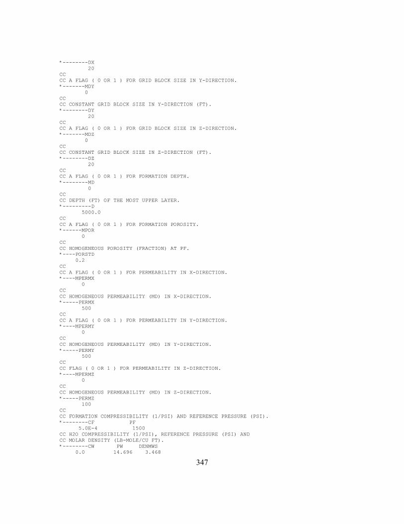
347
*--------DX 20 CC CC A FLAG ( 0 OR 1 ) FOR GRID BLOCK SIZE IN Y-DIRECTION. *-------MDY 0 CC CC CONSTANT GRID BLOCK SIZE IN Y-DIRECTION (FT). *--------DY 20 CC CC A FLAG ( 0 OR 1 ) FOR GRID BLOCK SIZE IN Z-DIRECTION. *-------MDZ 0 CC CC CONSTANT GRID BLOCK SIZE IN Z-DIRECTION (FT). *--------DZ 20 CC CC A FLAG ( 0 OR 1 ) FOR FORMATION DEPTH. *--------MD 0 CC CC DEPTH (FT) OF THE MOST UPPER LAYER. *---------D 5000.0 CC CC A FLAG ( 0 OR 1 ) FOR FORMATION POROSITY. *------MPOR 0 CC CC HOMOGENEOUS POROSITY (FRACTION) AT PF. *----PORSTD 0.2 CC CC A FLAG ( 0 OR 1 ) FOR PERMEABILITY IN X-DIRECTION. *----MPERMX 0 CC CC HOMOGENEOUS PERMEABILITY (MD) IN X-DIRECTION. *-----PERMX 500 CC CC A FLAG ( 0 OR 1 ) FOR PERMEABILITY IN Y-DIRECTION. *----MPERMY 0 CC CC HOMOGENEOUS PERMEABILITY (MD) IN Y-DIRECTION. *-----PERMY 500 CC CC FLAG ( 0 OR 1 ) FOR PERMEABILITY IN Z-DIRECTION. *----MPERMZ 0 CC CC HOMOGENEOUS PERMEABILITY (MD) IN Z-DIRECTION. *-----PERMZ 100 CC CC FORMATION COMPRESSIBILITY (1/PSI) AND REFERENCE PRESSURE (PSI). *--------CF PF 5.0E-4 1500 CC H2O COMPRESSIBILITY (1/PSI), REFERENCE PRESSURE (PSI) AND CC MOLAR DENSITY (LB-MOLE/CU FT). *--------CW PW DENMWS 0.0 14.696 3.468

348
CC CC WATER MOLECULAR WT. (LBM/LBM-MOLE) AND VISCOSITY (CP). *-------WTW VISCW 18. 1.0 CC CC FORMATION TEMPERATURE (F). *-----TEMPF 220.0 CC CC STANDARD TEMPERATURE (F) AND STANDARD PRESSURE (PSI). *-----TFSTD PSTD 60. 14.696 CC CC A FLAG ( 1, 2, 3 OR 4 ) FOR NUMERICAL DISPERSION CONTROL. *----IUPSTW 1 CC CC ITC ( 0 : NO 2ND ORDER TIME, 1 : 2ND ORDER TIME ON ) *----ITC 0 CC RESTART OPTIONS. CC ISTART ( 1 OR 2 ), ISTORE ( 0 OR 1 ). *----ISTART ISTORE 1 0 CC CC A FLAG ( 0 OR 1 ) FOR AUTOMATIC TIME-STEP SELECTION ( = 1 ). *-------MDT 1 CC CC A FLAG ( 0 OR 1 ) FOR PHYSICAL DISPERSION CALCULATION. *-----MDISP 0 CC FLAGS FOR RELATIVE PERMEABILITY MODEL AND CAPILLARY PRESSURE. CC IPERM ( 1 OR 2 ), ICPRES ( 0 OR 1 ). *-----IPERM ICPRES ICAP IRPERM 4 0 2 0 CC CAPILLARY PRESSURE PARAMETERS AND CC WATER/OIL INTERFACIAL TENSION (DYNES/CM). *-------EPC CPC RIFTWO RIFTWG RIFTWL 2. 2.0 0. 0. 0. CC CC HIGH IFT RESIDUAL SATURATIONS. *------S1RW S2RW1 S2RW2 S3RW S4RW1 S4RW2 0.2 .1 .0 0.0 0.0 0.0 CC CC LOW IFT RESIDUAL SATURATIONS. *------S1RC S2RC1 S2RC2 S3RC S4RC1 S4RC2 0.2 .1 .0 0.0 0.0 0.0 CC CC HIGH IFT END POINT RELATIVE PERMEABILITY. *------P1RW P2RW P3RW P4RW 0.4 1.0 1.0 1.0 CC CC LOW IFT END POINT RELATIVE PERMEABILITY. *------P1RC P2RC P3RC P4RC 0.4 1.0 1.0 1.0 CC CC HIGH IFT EXPONENT OF RELATIVE PERMEABILITY. *-------E1W E2W1 E2W2 E3W E4W1 E4W2 3.0 2.0 2.0 1.0 1.0 1.0 CC CC LOW IFT EXPONENT OF RELATIVE PERMEABILITY. *-------E1C E2C1 E2C2 E3C E4C1 E4C2 3.0 2.0 2.0 1.0 1.0 1.0 CC CC WATER AND L1 PHASE CAPILLARY DESATURATION PARAMETERS.

349
*-------T11 T12 T211 T221 T212 T222 250. 1. 3000. 1. 3000. 1. CC CC GAS AND L2 PHASE CAPILLARY DESATURATION PARAMETERS. *-------T31 T32 T411 T421 T412 T422 0. 0. 0. 0. 0. 0. C CC A FLAG FOR PRESSURE EQUATION SOLVER ( 1, 2, 3, 4 OR 5 ). *----IPRESS IPREC METHSL OMEGA 4 2 1 1.0 CC CC ITERATIVE PRESSURE SOLVER PARAMETERS. *-----ITMAX LEVLIT IDGTS NS1 NS2 ZETA 1000 1 -1 5 1000000 1.E-07 CC CC INITIAL TIME (DAYS). *---------T 0 CC CC A FLAG ( 0 OR 1 ) FOR INITIAL PRESSURE. *--------MP 0 CC CC CONSTANT INITIAL PRESSURE (PSIA). *---------P 5000.0 CC CC A FLAG ( 0 OR 1 ) FOR INITIAL WATER SATURATION. *------MSAT 0 CC CC CONSTANT INITIAL WATER SATURATION (FRACTION). *-------SAT 0.2 CC CC A FLAG ( 0 OR 1 ) FOR INITIAL OVERALL COMPOSITION. *-----MOMFR 0 CC CC CONSTANT INITIAL COMPOSITION (MOLE FRACTION). *------OMFR 0.0246 0.4041 0.0755 0.2719 0.1064 0.0774 0.0401 CC CC*********************************************************************** CC * CC RECURRENT DATA * CC * CC*********************************************************************** CC CC CC MAXIMUM TIME (DAYS), TIME STEP (DAYS) AND WELL DATA. *----TM DT NWELLS GORLIM WORLIM 60.0 0.05 2 -1. -1. CC CC PARAMETERS FOR TIME STEP SELECTORS. *-----DTMAX DTMIN DSLIM DPLIM DVLIM DMFACT 0.1 1e-5 0.05 0.01 .05 .05 CC CC WELL NO. AND WELL TYPE. *--------LW IQTYPE IWELLBORE (0:OFF, 1:0N) 1 -5 1 CC CC (MOLES/D) *----QTMLC(1) FWMLC(1) NCOMP ISWITCH PBHC 1000 CC

350
CC WELL NO. AND WELL TYPE. *--------LW IQTYPE IWELLBORE (0:OFF, 1:0N) 2 2 0 CC CC (MOLES/D) *----P FWMLC(1) NCOMP 100 0 1 CC CC INJECTION COMPONENT NO. AND COMPOSITION (FRACTION). NCOMP CARDS. *--------KC Z1 1 1 CC CC END OF INPUT. *--------TM DT NWELLS GORLIM WORLIM ---------------- -1. -1. -1. -1.E10 -1.E10 CC ==================================================================* CC WELLBORE MODEL INPUT DATA * CC ================================================================= * CC * CC CASE NAME: 7COMP ASPHALTENE FLUID PROD WELL (BURK ETAL DATA) * CC CREATED BY: Mahdy Shirdel 11/15/2012 * CC * CC ==================================================================* CC CC******************************************************************** CC WELL #01 DATA * CC******************************************************************** CC CC CASE DEFINITION: {WELL ID} *-----LW WELL NAME 1 TEST CC CC MESH GRID SIZE *--------MAX_GRID_SIZE[FT] 200.0 CC CC WELL SURFACE *--------WSURFACE[FT] 0.0 CC CC WELL PROFILE AND SURVEY *--------INTERVAL MD[FT] TVD[FT] INCLINATION[DEGREE] AZIMUTH[DEGREE] 1 5000 5000 90 0 CC CC WELL CASING AND COMPLETION {Default RWB=RCO+0.041665} (CODE:7") *--------INTERVAL HANGER_DEPTH[FT] SETTING_DEPTH[FT] RCI[FT] RCO[FT] RWB[FT] CEMENT_TOP[FT] EPSCI EPSCO KCASE[BTU/HR.FT.F] KCEM[BTU/HR.FT.F] HC ANNULUS_FLUID_ID [SELECT FROM TABLE] 1 0 50 0.78 0.833 0.8749 0 0.9 0.9 26 4.02 1.0 19 2 0 1000 0.51722 0.55725 0.59891 0 0.9 0.9 26 4.02 1.0 19 3 0 5000 0.3648 0.4010 0.4427 0 0.9 0.9 26 4.02 1.0 19 CC CC WELL OPEN HOLE *--------OPENHOLE_LENGTH[FT] OPENHOLE_RWB[FT] OPENHOLE_ROUGHNESS[FT/FT] 0 0.3333 0.0 CC CC WELL TUBING COMPLETION (CODE:API 3 1/2" )(0.1 ft Black Aerogel) *--------INTERVAL TUBE_TOP[FT] TUBE_BOTT[FT] RTI[FT] RTO[FT] EPSTO KTUB[BTU/HR.FT.F] INS_THICKNESS[FT] KINS[BTU/HR.FT.F] HC ANNULUS_FLUID_ID ROUGHNESS
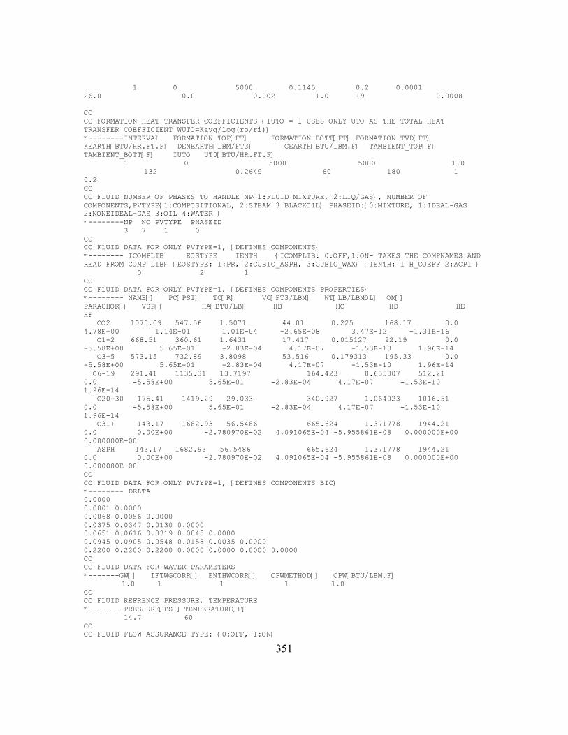
351
1 0 5000 0.1145 0.2 0.0001 26.0 0.0 0.002 1.0 19 0.0008 CC CC FORMATION HEAT TRANSFER COEFFICIENTS {IUTO = 1 USES ONLY UTO AS THE TOTAL HEAT TRANSFER COEFFICIENT WUTO=Kavg/log(ro/ri)} *--------INTERVAL FORMATION_TOP[FT] FORMATION_BOTT[FT] FORMATION_TVD[FT] KEARTH[BTU/HR.FT.F] DENEARTH[LBM/FT3] CEARTH[BTU/LBM.F] TAMBIENT_TOP[F] TAMBIENT_BOTT[F] IUTO UT0[BTU/HR.FT.F] 1 0 5000 5000 1.0 132 0.2649 60 180 1 0.2 CC CC FLUID NUMBER OF PHASES TO HANDLE NP{1:FLUID MIXTURE, 2:LIQ/GAS}, NUMBER OF COMPONENTS,PVTYPE{1:COMPOSITIONAL, 2:STEAM 3:BLACKOIL} PHASEID:{0:MIXTURE, 1:IDEAL-GAS 2:NONEIDEAL-GAS 3:OIL 4:WATER } *--------NP NC PVTYPE PHASEID 3 7 1 0 CC CC FLUID DATA FOR ONLY PVTYPE=1, {DEFINES COMPONENTS} *-------- ICOMPLIB EOSTYPE IENTH {ICOMPLIB: 0:OFF,1:ON- TAKES THE COMPNAMES AND READ FROM COMP LIB} {EOSTYPE: 1:PR, 2:CUBIC_ASPH, 3:CUBIC_WAX} {IENTH: 1 H_COEFF 2:ACPI } 0 2 1 CC CC FLUID DATA FOR ONLY PVTYPE=1, {DEFINES COMPONENTS PROPERTIES} *-------- NAME[] PC[PSI] TC[R] VC[FT3/LBM] WT[LB/LBMOL] OM[] PARACHOR[] VSP[] HA[BTU/LB] HB HC HD HE HF CO2 1070.09 547.56 1.5071 44.01 0.225 168.17 0.0 4.78E+00 1.14E-01 1.01E-04 -2.65E-08 3.47E-12 -1.31E-16 C1-2 668.51 360.61 1.6431 17.417 0.015127 92.19 0.0 -5.58E+00 5.65E-01 -2.83E-04 4.17E-07 -1.53E-10 1.96E-14 C3-5 573.15 732.89 3.8098 53.516 0.179313 195.33 0.0 -5.58E+00 5.65E-01 -2.83E-04 4.17E-07 -1.53E-10 1.96E-14 C6-19 291.41 1135.31 13.7197 164.423 0.655007 512.21 0.0 -5.58E+00 5.65E-01 -2.83E-04 4.17E-07 -1.53E-10 1.96E-14 C20-30 175.41 1419.29 29.033 340.927 1.064023 1016.51 0.0 -5.58E+00 5.65E-01 -2.83E-04 4.17E-07 -1.53E-10 1.96E-14 C31+ 143.17 1682.93 56.5486 665.624 1.371778 1944.21 0.0 0.00E+00 -2.780970E-02 4.091065E-04 -5.955861E-08 0.000000E+00 0.000000E+00 ASPH 143.17 1682.93 56.5486 665.624 1.371778 1944.21 0.0 0.00E+00 -2.780970E-02 4.091065E-04 -5.955861E-08 0.000000E+00 0.000000E+00 CC CC FLUID DATA FOR ONLY PVTYPE=1, {DEFINES COMPONENTS BIC} *-------- DELTA 0.0000 0.0001 0.0000 0.0068 0.0056 0.0000 0.0375 0.0347 0.0130 0.0000 0.0651 0.0616 0.0319 0.0045 0.0000 0.0945 0.0905 0.0548 0.0158 0.0035 0.0000 0.2200 0.2200 0.2200 0.0000 0.0000 0.0000 0.0000 CC CC FLUID DATA FOR WATER PARAMETERS *-------GW[] IFTWGCORR[] ENTHWCORR[] CPWMETHOD[] CPW[BTU/LBM.F] 1.0 1 1 1 1.0 CC CC FLUID REFRENCE PRESSURE, TEMPERATURE *--------PRESSURE[PSI] TEMPERATURE[F] 14.7 60 CC CC FLUID FLOW ASSURANCE TYPE: {0:OFF, 1:ON}

352
*-------- IASPH IWAX ISCALE 1 0 0 CC CC FLUID FLOW ASSURANCE ASPHALTENE ONSET DATA *-------- VBS[FT3/LBM] KCOND_ASPH KS1S2 IDEPOSIT DPS1[cm] DPS2 KD_LMNAR[cm/SEC] KDS1 KDS2 EAS1 EAS2[KJ] 10.3 1.0 0.0 4 5.0E-6 5.0E-6 1.0E11 1.0E9 1.0E9 65.3 65.3 CC CC FLUID FLOW ASSURANCE ASPHALTENE ONSET DATA *-------- NONSET PSTAR[PSI] TSTAR[F] 1 4600 212 2 5046 200 3 5451 190 4 5961 180 5 6659 170 6 7581 160 7 8650 150 8 9543 145 CC CC RESERVOIR COUPLING: {0: STATIC, 1:DYNAMIC} *-------- IRESERVOIR 1 CC CC PROCESS CONDITIONS *-------- IPROD[] {1:INJECTION, -1:PRODUCTION} ITHERMAL[] ITRANSIENT[] IMODEL[]{0:no slip, 1:drift flux, 2:two-fluid} ISLIPOW[] ISLIPGL[] -1 1 0 0 0 0 CC CC INITIAL CONDITIONS {ZERO IS STATIONARY EQUILIBRIUM WITH RESERVOIR} *-------- TINIT[F] PINIT[PSI] HLDPHC[] HLDPW[] UGINIT[FT/SEC] UOINIT[FT/SEC] UWINIT[FT/SEC] 0.0 0.0 0.01 0.01 0.0 0.0 0.0 CC CC OUTPUT PRINT FREQUENCY * ------TPRNT 1 CC CC OUTPUT PVT PLOTS {0: OFF, 1:ON} * ------ IPVT TEMP1[F] TEMP2[F] PRES1[PSI] PRES2[PSI] 0 120 600 500 2500 CC CC NUMERICAL CONVERGENCE TOLERRANCE *--------WTOLP[PSIA] WTOLT[F] WTOLQ[LBM/HR] WMAXITER 0.1 0.1 0.1 20 CC CC NUMERICAL SIMULATION TIME *--------START_TIME[DAY] END_TIME [DAY] DTMIN[DAY] DTMAX[DAY] {TIME STEP SIZE SHOUDL BE SETUP LESS THAN TIME INTERVALS FOR RESERVOIR CONDITION} 0.0 30 0.1 0.1 CC CC END OF INPUT.

353
G.6 PHREEQC SAMPLE DATABASE
#*********************************************** #***************WATER*************************** #*********************************************** SOLUTION_MASTER_SPECIES H H+ -1. H 1.008 H(0) H2 0.0 H H(1) H+ -1. 0.0 E e- 0.0 0.0 0.0 O H2O 0.0 O 16.00 O(0) O2 0.0 O O(-2) H2O 0.0 0.0 #************************************************* #************************************************* Ca Ca+2 0.0 Ca 40.08 Na Na+ 0.0 Na 22.9898 Ba Ba+2 0.0 Ba 137.34 Cl Cl- 0.0 Cl 35.453 C CO3-2 2.0 HCO3 12.0111 C(+4) CO3-2 2.0 HCO3 S SO4-2 0.0 SO4 32.064 S(6) SO4-2 0.0 SO4 #************************************************* #************************************************* #************************************************* SOLUTION_SPECIES e- = e- log_k 0.000 H2O = H2O log_k 0.000 -gamma 10e9 0.0 H+ = H+ log_k 0.000 -gamma 10e9 0.0 H2O = OH- + H+ log_k -14.000 -gamma 10e9 0.0 2 H2O = O2 + 4 H+ + 4 e- log_k -86.08 2 H2O = O2 + 4 H+ + 4 e- log_k -86.08 2 H+ + 2 e- = H2 log_k -3.15 #*************************************************

354
#************************************************* H+ = H+ log_k 0.000 Na+ = Na+ log_k 0.000 -gamma 10e9 0.0 Ba+2 = Ba+2 log_k 0.000 -gamma 10e9 0.0 Ca+2 = Ca+2 log_k 0.000 -gamma 10e9 0.0 Cl- = Cl- log_k 0.000 -gamma 3.5000 0.0150 SO4-2 = SO4-2 log_k 0.000 -gamma 10e9 0.0 CO3-2 = CO3-2 log_k 0.000 -gamma 5.4000 0.0000 CO3-2 + H+ = HCO3- log_k 10.329 -gamma 5.4000 0.0000 CO3-2 + 2 H+ = CO2 + H2O log_k 16.681 Ba+2 + SO4-2 = BaSO4 log_k 2.700 Ba+2 + CO3-2 = BaCO3 log_k 2.71 Ca+2 + SO4-2 = CaSO4 log_k 2.300 Ca+2 + CO3-2 = CaCO3 log_k 3.224 #************************************************* #************************************************* #************************************************* PHASES Calcite CaCO3 = CO3-2 + Ca+2 log_k -8.480 Witherite BaCO3 = Ba+2 + CO3-2

355
log_k -8.562 Barite BaSO4 = Ba+2 + SO4-2 log_k -14.85 Anhydrite CaSO4 = Ca+2 + SO4-2 log_k -14.480000

356
G.7 PHREEQC SAMPLE INPUT DATA
PRINT -RESET TRUE SELECTED_OUTPUT -RESET FALSE USER_PUNCH -headings Ca -headings Ba -headings Na -headings Cl -headings S(6) -headings C(+4) -headings Ca+2 -headings Ba+2 -headings Na+ -headings CO3-2 -headings HCO3- -headings CO2 -headings SO4-2 -headings BaSO4 -headings BaCO3 -headings CaSO4 -headings CaCO3 -headings Anhydrite -headings Calcite -headings Witherite -headings Barite -start 10 PUNCH TOT("Ca") 20 PUNCH TOT("Ba") 30 PUNCH TOT("Na") 40 PUNCH TOT("Cl") 50 PUNCH TOT("S(6)") 60 PUNCH TOT("C(+4)") 70 PUNCH MOl("Ca+2") 80 PUNCH MOL("Ba+2") 90 PUNCH MOL("Na+") 100 PUNCH MOL("CO3-2") 120 PUNCH MOL("HCO3-") 120 PUNCH MOL("CO2") 130 PUNCH MOL("SO4-2") 140 PUNCH MOL("BaSO4") 150 PUNCH MOL("BaCO3") 160 PUNCH MOl("CaSO4") 170 PUNCH MOl("CaCO3") 180 PUNCH EQUI("Anhydrite") 190 PUNCH EQUI("Calcite") 200 PUNCH EQUI("Witherite") 200 PUNCH EQUI("Barite") -end TITLE FOUR SCALE PERCIPITATION SOLUTION 1 -units mol/kgw -pH 7.0 -temp 25.0

357
Ca 0.0500 Ba 0.0500 Na 0.2000 Cl 0.2000 S(6) 0.0500 C(+4) 0.0500 REACTION_TEMPERATURE 1 50.0 EQUILIBRIUM_PHASES Anhydrite 0. 0.000000E+00 Calcite 0. 0.000000E+00 Witherite 0. 0.000000E+00 Barite 0. 0.000000E+00 END

358
Glossary
The following list of nomenclature includes only the generalized symbols used in
the text. Symbols which have been used to represent different quantities have been
defined as they were used in the text.
A Wellbore / pipe cross section area (ft2) B Gravity force gradient (ft/sec2) Bo Oil formation volume factor (rbbl/stb)
vmC Virtual mass parameter 0C Drift flux profile parameter
Cb Average bulk particle concentration (lbm/ft3) Cs Average surface particle concentration (lbm/ft3) D Wellbore/pipe diameter (ft)
BD Brownian diffusivity (m2/sec) pipeD Non-dimensional pipe diameter
pd Particle diameter (m) f Friction factor
fi Fugacity of component i in the hydrocarbon mixture FIG Interphase gas friction force factor (1/sec) FIL Interphase liquid friction force factor (1/sec) FWG Wall/Gas friction force factor (1/sec) FWL Wall/Liquid friction force factor (1/sec) g Gravity acceleration (ft/sec2) h Fluid height in the cross section (ft) h Fluid enthalpy (Btu/lbm) j Spatial variable numerical index (junction) K Spatial variable node center index
tK Transport coefficient (m/sec) L Spatial variable node center index M Spatial variable node center index dm Mass deposition flux (lbm/sec. ft2)

359
n Time variable numerical index kN Molar per bulk volume of hydrocarbon component k in the mixture (lbmol /ft3)
cn Number of hydrocarbon components P Pressure (psi) Q Wellbore gridblock heat loss (Btu/sec.ft)
sR Solution gas oil ratio (scf/stb) avgr Non-dimensional average radial distance
S Wellbore wetted perimeter (ft) SP Sticking probability pS Non-dimensional stopping distance
T Temperature (oF) t Time variable (sec) u Actual velocity (ft/sec) v Drift velocity (ft/sec) VISL Liquid viscous -like term in momentum equation VISG Gas viscous-like term in momentum equation Vb Wellbore grid bulk volume (ft3) x Well trajectory spatial variable (ft) y Liquid height from center of pipe (ft) y Non-dimensional distance from the wellbore / pipe wall
z Wellbore gridblock overall composition of fluid mixture Greek Symbols Fluid volume fraction Fluid mass influx per gridblock bulk volume (lbm/ft3.sec) Fluid enthalpy influx per gridblock bulk volume (Btu/ ft3.sec) Fluid density (lbm/ft3) Liquid/gas interfacial tension Viscosity (Cp) Well trajectory angle (radian) Shear stress (lbm/sec2.ft) Interphase mass transfer per bulk volume (lbm/sec.ft3) Subscripts d Drift
360
g Gas gi Gas interphase i Interphase l Liquid li Liquid interphase m Mixture mx Maximum o Oil TB Taylor bubble sl Superficial variable for liquid phase (i.e. superficial liquid velocity) sg Superficial variable for gas phase sp Single phase tp Two phase w Water

361
References
Akbarzadeh, K., Hammami, A., Kharrat, A., Zhang, D., Allenson, S., Creek, J., Kabir, S.,
Jamaluddin, A., Marshall, A.G., Rodgers, R.P., Mullins, O.C., and Solbakken, T.: “Asphaltene – Problematic but Rich in Potential,” Schlumberger Oil Field Review, pp. 22- 43, Summer 2007.
Ali, M.A. and Islam, M.R.: “The Effect of Asphaltene Precipitation on Carbonate-Rock
Permeability: An Experimental and Numerical Approach,” SPE Production and Facilities, pp. 178– 183, Aug 1998.
Almehaideb, R.A., Aziz, K., and Pedrosa Jr., O.J.: “A Reservoir/Wellbore Model for
Multiphase Injection and Pressure Transient Analysis,” Paper SPE 17941, presented at 6th Middle East Oil Technical Conference and Exhibition, Manama, Bahrain, Mar 11-14, 1989.
Ansari, A.M., Sylvester, N.D., Sarica, C., Shoham, O., and Brill, J. P.: “A
Comprehensive Mechanistic Model for Upward Two-Phase Flow in Wellbores,” SPE Production & Facilities Journal, pp. 143-151, 1994.
Aziz, K., Govier, G.W., and Fogarasi, M.: “Pressure Drop in Wells Producing Oil and
Gas,” JCPT, pp. 38-47, July-Sept 1972. Babu, D.K. and Odeh, A.S.: “Productivity of a Horizontal Well,” Soc. Pet. Eng.
Reservoir Eng., 4, pp. 417-421, Nov 1989. Baker, O. and Swerdloff, W.: “Calculation of Surface Tension,” Oil and Gas Journal,
141, Dec 1955. Barnea, D., Shoham, O., and Taitel, Y.: “Flow Pattern Transition for Vertical Downward
Two-Phase Flow,” Chem. Eng. Sci., 37, pp. 741, 1982. Banerjee, S. and Chan, A.M.C.: “Separated Flow Models I. Analysis of the Averaged and
Local Instantaneous Formulations,” International Journal of Multiphase Flow, 6, pp.124, 1980.
Beal, S., K.: “Deposition of Particles in Turbulent Flow on Channel or Pipe Walls,”
Nuclear Science and Engineering, 40, pp. 1-11, 1970. Bedrikovestsky, P.G., Lopes, R.P. Jr., Rosario, F.F., Bezerra, M.C., and Lima, E.A.:
“Oilfield Scaling Part I: mathematical and Laboratory Modeling,” Paper SPE 81127,

362
Presented at the Latin American and Caribbean Petroleum Engineering conference, Port-of-Spain, Trinidad, West India, pp. 27-30, Apr 2003.
Behie, A., Collins, D., Forsyth, P.A., and Sammon, P.H.: “Fully Coupled Multiblock
Wells in Oil Simulation,” Paper SPE 11877, Journal of Petroleum Technology, pp. 535-542, Aug 1985.
Beggs, H.D. and Brill, J.P.: “A Study of Two-Phase Flow in Inclined Pipes,” Journal of
Petroleum Technology, pp. 607-617, May 1973. Beggs, H.D. and Robinson, J.R.: “Estimating the Viscosity of Crude Oil Systems,”
Journal of Petroleum Technology, 27, pp. 1140–1141, Sep 1975. Bendiksen, K.H., Malnes, D., Moe, R., and Nuland, S.: “The Dynamic Two-Fluid Model
OLGA: Theory and Application,” SPE Production Engineering, 6, pp. 171-180, May 1991.
Benedict, M., Webb, G.B., and Rubin L.C.: “An Empirical Equation for Thermodynamic
Propertied of Light Hydrocarbons and their Mixture,” Journal of Chem. Phys, 8, pp. 334-45, 1940.
Bird, R., B., Stewart, W., and E., Lightfoot, E., N.: Transport Phenomena, 2nd Edition,
John Wiley & Sons, 2002. Brown, T.S., Niesen, V.G., and Erickson, D.D.: “Measurement and Prediction of Kinetics
of Paraffin Deposition,” Paper SPE 26548, 68th Annual Technical Conference and Exhibition, Houston, TX, Oct 3-6, 1993.
Burke, N.E., Hobbs, R.D., and Kashou, S.F.: "Measurement and Modeling of Asphaltene
Precipitation,” JPT, pp. 1440-1446, 1990. Carbognani, L., Orea, M., and Fonseca, M.: “Complex Nature of Separated Solid Phases
from Crude Oils,” Energy & Fuels, 13, pp. 351-358, 1999. Carnahan, N. F.: “Precipitation of Asphaltene in Heavy Oil and Tar Sands,” in
Asphaltenes and Asphalts, Elsevier Science B.V., 2000. Chang, Y.B.: “Development and application of an Equation of States Compositional
Simulator,” Ph.D. Dissertation, The University of Texas at Austin, 1990. Chapman, W.G, Gubbins, K.E., Jackson, G., and Radosz, M.: “New Reference Equation
of State for Associating Liquids,” Ind. Eng. Chem. Res., 29(8), pp. 1709-1721, 1990.

363
Chokshi, R.N: “Prediction of Pressure Drop and Liquid Holdup in Vertical Two-Phase Flow through Large Diameter Tubing,” Ph.D. Dissertation, The University of Tulsa, 1994.
Chung, T.H.: “Thermodynamic Modeling for Organic Solid Precipitation,” Paper SPE
24851, Washington D.C, USA, Oct. 4-7, 1992. Cleaver, J., W. and Yates, B.: “A Sub-layer Model for the Deposition of Particles from a
Turbulent Flow,” Chem. Eng. Sci., 30, pp. 983-992, 1975. Crabtree, M.: “Fighting Scale-Removal and Prevention,” Schlumberger Oilfield Review,
pp. 30-40, Autumn 1999. Darabi, H., Sepehrnoori, K., and Kalaei, H.: “Modeling of Wettability Alteration Due to
Asphaltene Deposition in Oil Reservoirs,” SPE Paper 159554, Presented at Annual Technical Conference and Exhibition, San Antonio, Texas, USA, Oct 8-10, 2012.
Davis, J.T.: “A New Theory of the Deposition of Colloidal Particles from Turbulent
Fluids,” Annals of the New York Academy of Science, 404, pp. 313-326, 1983. Dinh, T.N., Nourgaliev, R.R., and Theofanous, T.G.: “Understanding The Ill-posed Two-
Fluid Model,” NURETH, Seoul, Korea, Oct 59, 2003. De Ghetto, G., Paone F., and Villa M.: “Reliability Analysis on PVT Correlations,” Paper
SPE 28904, Presented at the European Petroleum Conference, London, UK, Oct 25-27, 1994.
Delshad, M. and Pope, G.: “Effect of Dispersion on Transport and Precipitation of
Barium and Sulfate in Oil Reservoirs,” SPE Paper 80253, Presented at the International Symposium on Oilfield Scale, Houston, Feb 5-8, 2003.
Dranchuk, P.M. and Abou-Kassem, J.H.: “Calculation of Z-factor for Natural Gases
Using Equations of State,” Journal of Canadian Petroleum Technology, 34, Jul 1975. Drew, D. A. and Lahey, R.T.: “Application of General Constitutive Principles to the
Derivation of Multidimensional Two-Phase Flow Equations,” Int. J. Multiphase Flow, Vol.5, pp.243264, 1979.
Dukler, A.E., Wicks. M. III., and Cleveland, R.G.: “Frictional Pressure Drop in Two-
Phase Flow: An Approach through Similarity Analysis,” AIChE Journal, 10, 44, 1964.
Duns, H.Jr. and Ros, N.C.J.: “Vertical Flow of Gas and Liquid Mixtures in Wells,” Paper
22-PD6 of the Sixth World Petroleum Congress, Frankfurt, Germany, Jun 1963.

364
Eaton, B.A., Andrews, D.E., Knowles, C.R., Silberberg, I.H., and Brown, K.E.: “The Prediction of Flow Patterns, Liquid Holdup and Pressure Losses Occurring During Continuous Two-Phase Flow in Horizontal Pipelines,” Journal of Petroleum Technology, pp. 815, Jun 1967.
Egbogah, E.O. and Ng, J.T..: “An Improved Temperature-Viscosity Correlation for
Crude Oil Systems,” Journal of Petroleum Science and Engineering, 4, pp. 197-200, Jul 1990.
Erickson, D.D., Niesen, V.G., and Brown, T.S.: “Thermodynamic Measurement and
Prediction of Paraffin Precipitated in Crude Oil,” Paper SPE 26604, Presented at SPE ATCE, Houston, TX, Oct 3-6, 1993.
Erickson, D.D. and Mai, M.C.: “A Transient Multiphase Temperature Prediction
Program,” Paper SPE 24790, Presented at SPE ATCE, Washington D.C, Oct 4-7, 1992.
Epstein, N.: “Particulate Fouling of Heat Transfer Surface: Mechanisms and Models”
Fouling Science and Technology, 145, pp. 143-164, 1988. Escobedo, J.: “Mexican Crude Oils and the Asphaltene Deposition Problem” M.Sc.
thesis, The University of Illinois at Chicago, Chicago, IL, 1993. Escobedo, J. and Mansoori, G.A.: “Asphaltene and Other Heavy-Organic Particle
Deposition during Transfer and Production Operation,” Paper SPE 29488, Production Operation Symposium, Oklahoma City, Oklahoma, USA, Apr 2-4, 1995.
Eskin, D., Ratulowski, J., Akbarzadeh, K., and Pan, S.: “Modeling Asphaltene
Deposition in Turbulent Pipeline Flows,” The Canadian Journal of Chemical Engineering , pp. 421-441, June, 2011.
Fair, W.B. Jr.: “Pressure Buildup Analysis with Wellbore Phase Redistribution,” Paper
SPE 8206, SPE Journal, 21, 2, pp. 259-270, Apr 1981. Fan, L., Lee, W.J., and Spivey, J.P.: “Semi-Analytical Model for Thermal Effect on Gas
Well Pressure Buildup Tests,” Paper SPE 56612, presented at SPE Annual Technical Conference and Exhibition, Houston, Texas, Oct 3-6, 2000.
Fazelipour, W.: “Development of a Fully Implicit, Parallel, Equation-of-State
Compositional Simulator to Model Asphaltene Precipitation in Petroleum Reservoirs,” M.Sc. Thesis, the University of Texas at Austin, 2007.
Friedlander, S.K. and Johnstone, H.F.: “Deposition of Suspended Particles from
Turbulent Gas Streams,” Ind. Eng. Chem., 49, pp. 1151-1156, 1957.

365
Frenier., W. and Ziauddin, M.: Formation, Removal, and Inhibition of Inorganic Scale in the Oilfield Environment, SPE Book, pp.59-85, 2008.
Gambill, W. R.: “You Can Predict Heat Capacities,” Chemical Engineering, pp. 243–248,
Jun 1957. Gidaspow, D.: “Modeling of Two Phase Flow,” Proceedings of the 5th International Heat
Transfer Conference VII, 1974. Gomez, L.E., Shoham, O., and Taitel, Y.: “Prediction of Slug Liquid Holdup-Horizontal
to Upward Vertical Flow,” International Journal of Multiphase Flow, 26, 3, pp. 517, Mar 2000.
Gonzalez, D.L, Ting, P.D., and Hirasaki, G.J., Chapman, W.G.: “Prediction of
Asphaltene Instability under Gas Injection with the PC-SAFT Equation of State,” Energy & Fuels, 19(4), pp. 1230-1234, 2005.
Gonzalez, D.L., Hirasaki, G.J., Creek, J., and Chapman, W.G.: “Modeling of Asphaltene
Precipitation Due to Changes in Composition Using the Perturbed Chain Statistical Associating Fluid Theory Equation of State,” Energy & Fuels, 21(3), pp. 1231-1242, 2007.
Gross, J. and Sadowski, G.: “Perturbed-Chain SAFT; An Equation of State Based on a
Perturbation Theory for Chain Molecules,” Ind. Eng. Chem. Res., 40(4), pp. 1244-1260, 2001.
Hagedorn, A.R. and Brown, K.E.: “Experimental Study of Pressure Gradients Occurring
During Continuous Two-Phase Flow in Small-Diameter Vertical Conduits,” Journal of Petroleum Technology, pp. 475, Apr 1965.
Hammami, A., Ferworn, K.A., Nighswander, J.A., Overa, S., and Stange, E.:
“Asphaltenic Petroleum Fluid Oil Characterization: An Experimental Investigation of the Effect of Resins on the Stability of Asphaltenes,” Pet. Sci. Technol., 16(3– 4), 227, 1998.
Hamouda, A.: “An Approach for Simulation of Paraffin Deposition in Pipelines as a
Function of Flow Characteristics with a Reference to Teesside Oil Pipeline,” Paper SPE 28966, Presented at SPE Int. Symposium on Oilfield Chemistry, San Antonio, 14-17, Feb 1995.
Han, C., Delshad, M., Sepehrnoori, K., and Pope, G.: “A Fully Implicit, Parallel,
Compositional Chemical Flooding Simulator,” Society of Petroleum Engineering Journal, 12, 3, pp. 322-338, 2007.

366
Hasan, A.R. and Kabir, C.S.: “A Study of Multiphase Flow Behavior in Vertical Wells,” SPE Production Engineering Journal, pp. 263–272, May 1988.
Hasan, A.R. and Kabir, C.S.: “Predicting Multiphase Flow Behavior in Deviated Wells,”
SPE Production Engineering Journal, pp. 474–482, Nov 1988. Hasan, A.R. and Kabir, C.S.: “A Wellbore/Reservoir Simulator for Testing Gas Wells in
High-Temperature Reservoirs,” SPE Formation Evaluation Journal, pp. 128-135, Jun 1996.
Hasan, A.R. and Kabir, C.S.: “A Mechanistic Model for Computing Fluid Temperature
Profiles in Gas-Lift Wells,” SPE Production Facilities Journal, pp. 179, Aug 1996. Hasan, A.R., Kabir, C.S., and Wang, X.: “Development and Application of a
Wellbore/Reservoir Simulator for Testing Oil Wells,” SPE Formation Evaluation Journal, pp. 182-188, Sep 1997.
Hasan, A.R., Kabir, C.S., and Wang, X.: “Wellbore Two-Phase Flow and Heat Transfer
during Transient Testing,” Society of Petroleum Engineering Journal, 3, 2, pp. 174-180, Jun 1998.
Hasan, A.R., Kabir, C.S., and Sayarpour, M.: “A Basic Approach to Wellbore Two-Phase
Flow Modeling,” Paper SPE 109868, Presented at SPE Annual Technical conference and Exhibition, Anaheim, CA, USA, 11-14 Nov, 2007.
Haskett, C.E. and Tartera, M.: “A Practical Solution to the Problem of Asphaltene
Deposits – Hassi Messaoud Field, Algeria,” J. Pet. Tech., pp. 387-391, Apr 1965. Hayduk, W. and Minhas, B.S.: “Correlations for Predictions of Molecular Diffusivities in
Liquids,” The Canadian Journal of Chemical Engineering, 60, 295, 1982. Hernandez, O.C., Hensley, H., Sarica, C., Brill, J.P., Volk, M., and Delle-Case, E.:
“Improvements in Single-Phase Paraffin Deposition Modeling,” SPE Production and Facilities, 237, 2004.
Holman, J.P.: Heat Transfer, 4th ed., McGraw-Hill Book Co, New York, 1958. Hutchinson, P.C., Hewitt, G.F., and Dukler, A.E.: “Deposition of Liquid or Solid
Dispersions from Turbulent Gas Streams: A Stochastic Model,” Chem. Eng. Sci., 26, pp. 419-439, 1971.
Hwang, Y-H.: “Upwind Scheme for Non-Hyperbolic Systems,” J. Comput. Phys. 192,
pp. 643–676, 2003.

367
Issa, R.I. and Kempf, M.H.W.: “Simulation of Slug Flow in Horizontal and Nearly Horizontal Pipes with the Two-Fluid Model,” Int. J. Multiphase. Flow 29, pp. 69–95, 2003.
Ishii M.: "One-Dimensional Drift-flux Model and Constitutive Equations for Relative
Motion between Phases in Various Two-Phase Regimes,” Argonne National Laboratory, Oct 1977.
Ishii M. and Hibiki. T.: Thermo-fluid Dynamics of Two-Phase Flow, 2nd ed., Springer,
New York Dordrecht Heidelberg London, 2011. Johansen, S., T.: “The Deposition of Particles on Vertical Walls,” Int. J. Multiphase
Flow” 17, 3, pp. 355-376, 1991. Jarvis, S. J.: “On the Formulation and Numerical Evaluation of a Set of Two-Phase Flow
Equations Modeling the Cooldown Process,” Technical Note 301, National Bureau of Standards, Boulder, Colorado, 1965.
Jamialahmadi, M., Soltani, B., Muller-Steinhagen, H., and Rashtchian, D.: “Measurement
and Prediction of the Rate of Deposition of Flocculated Asphaltene Particles from Oil,” International Journal of Heat and Mass Transfer, 52, pp. 4624-4634, 2009.
Katz, D.L.: Handbook of Natural Gas Engineering, McGraw Hill Book Co., New York,
1959. Kaya, A.S, Sarica, C., and Brill J.P.: “Comprehensive Mechanistic Modeling of Two-
phase Flow in Deviated Wells,” Paper SPE 56522, Presented at Annual Technical Conference and Exhibition, Houston, Texas, Oct 3-6, 1999.
Kontogeorgis, G.M., Voutsas E.C., Yakoumis, I.V., and Tassios, D.P.: “An Equation of
State for Associating Fluids,” Ind. Eng. Chem. Res., 35(11), pp. -4318, Nov, 1996. Kohse, B.F, Nghiem, L.X, Maeda H., and Kenji, O.: “Modeling Phase Behavior
Including the Effect of Pressure and Temperature on Asphaltene Precipitation,” Paper SPE 64465, Presented at Asia Pacific Oil and Gas Conference and Exhibition, Brisbane, Australia, Oct 16-18, 2000.
Laufer, J., National Advisory Committee for Aeronautics, Technical Note, 2954, 1953. Lax, P.D.: “Differential Equations, Difference Equations and Matrix Theory,”
Communications on Pure and Applied Mathematics, Vol. XI, pp. 174-194, 1958. Lee, A.L., Gonzalez, M.H., and Eakin, B.E.: “The Viscosity of Natural Gases” Journal of
Petroleum Technology, pp. 997-1000, Aug 1966.

368
Leontaritis, K.J. and Mansoori, G.A.: “Asphaltene Deposition: A Survey of Field Experiences and Research Approaches,” J. of Pet. Sc. and Eng. 1, 229, 1988.
Lockhart, R. W. and Martinelli, R. C.: “Proposed Correlation of Data for Isothermal
Two-phase, Two-Component Flow in Pipes,” Chem. Eng. Prog., 45, 39, Jan 1949. Liao J., Mei, R., and Klausner, J.F: “A Study on the Numerical Stability of the Two-Fluid
Model Near Ill-posedness,” International Journal of Multiphase Flow 34, pp. 1067–1087, 2008.
Li, Z. and Firoozabadi, A.: “Cubic-Plus-Association (CPA) Equation of State for Water-
Containing Mixtures: Is ‘Cross Association” Necessary?,” AIChE J, 55(7), pp. 1803-1813, 2009.
Livescu, S., Durlofsky, L.J., and Aziz, K.: “Development and Application of a Fully-
coupled Thermal Compositional Wellbore Flow Model,” Paper SPE 121306, presented at the SPE Western Regional Meeting, San Jose, California, U.S.A., Mar 24-26, 2009.
Lichaa, P.M.: “Asphaltene Deposition Problem in Venezuela Crudes - Usage of
Asphaltenes in Emulsion Stability" Can. Pet. Tech. J., Oil Sands, pp. 609-624, 1977. Lin, C., S., Moulton, R., W., and Putnam, G., L.: “Mass Transfer between Solid and Fluid
Streams; Mechanism and Eddy Distribution Relationships in Turbulent Flow,” Ind. Eng. Chem, 45, pp. 636-640, 1953.
Lira-Galeana, C., Firoozabadi, A., and Prausnitz J.M.: “Thermodynamics of Wax
Precipitin in Petroleum Mixtures,” AIChE Journal, 42 (1), pp. 239-248, Jan 1996. Lohrenz, J., Bray, B.G., and Clark, C.R.: “Calculation Viscosities of Reservoir Fluids
from Their Composition,” Trans., AIME, V.142, pp. 159-172, 1964. Lyczkowski, R.W, Gidaspow, D., Solbrig, C.W., and Hughes, E.D.: “Fundamentals of
Two-Phase Flow,” Annual ASME Meeting, Houston, Nov. 30 – Dec. 4, 1975. Mamun, C.K.: “Free Energy of Mixing of Cross-linked Polymer Blemds,” Langmuir 21,
pp. 240-250, 2005. Mamun, C.K.: “Spatial Modulation in Cross-linked Binary Polymer Blends,” Langmuir,
21, pp. 7921-7936, 2005. Matzain, A.: “Multiphase Flow Paraffin Deposition Modeling,” Ph.D. Dissertation,
University of Tulsa, Tulsa, OK, 2001.

369
Micaelli, J.C.: “CATHARE an Advanced Best-Estimate Code for PWR Safety Analysis,” SEThiLEML-EM/87-58, 1987.
Mishima, K. and Ishii, M.: “Flow Regime Transition Criteria for Upward Two-Phase
Flow in Vertical Tubes,” International Journal of Heat and Mass Transfer, 27, pp. 723-737, 1984.
Mukherjee, H. and Brill, J.P.: “Liquid Holdup Correlations for Inclined Two-Phase
Flow,” Journal of Petroleum Technology, pp. 1003-1008, May 1983. Nancollas, G.H., White, W., Tsai, F., and Maslow, L.: “The Kinetics and Mechanism of
Formation of Calcium Sulfate Scale Minerals: the Influence of Inhibitors,” Corrosion, 35 (7), pp. 304-308, 1979.
Nghiem, L.X., Hassarn, M.S., and Nutakki, R.: “Efficient Modeling of Asphaltene
Precipitation,” SPE Paper 26642, Presented at Annual Technical Conference and Exhibition, Houston, Texas, Oct 3-6, 1993.
No, H.C. and Kazimi M.S.: “The Effect of Virtual Mass on the Characteristics and the
Numerical Stability in Two-Phase Flows,” MIT Energy Laboratory Report No. MIT-EL 81-023, April 1981.
Orkiszewski, J.: “Predicting Two-Phase Pressure Drops in Vertical Pipe,” Journal of
Petroleum Technology, pp. 829-838, Jun 1967. Ozon, P.M., Ferschneider, G., and Chwetzoff, A.: “A New Multiphase Flow Model
Predicts Pressure and Temperature Profile,” Paper SPE 16535, presented at the SPE Offshore Europe Conference, Aberdeen, Scotland, Sept. 8-11, 1987.
Papavergos, P., G. and Hedly, A., B.: “Particle Deposition Behaviour from Turbulent Gas
Streams,” Chem. Eng. Res. Des., 62, pp. 275-295, 1984. Parkhurst, D.L. and Appelo, C.A.J.: “Description of Input and Examples for PHREEQC
Version 3--A Computer Program for Speciation, Batch-Reaction, One-Dimensional Transport, and Inverse Geochemical Calculations,” U.S. Geological Survey Techniques and Methods, 2013.
Passut, C.A. and Danner, R.P.: “Correlation of Ideal Gas Enthalpy, Heat Capacity, and
Entropy,” Ind. Eng. Chem. Proc. Des. Development, 11, pp. 543-546, 1972. Peaceman, D.W.: “Interpretation of Well-Block Pressure in Numerical Reservoir
Simulation with Non-square Grid Blocks and Anisotropic Permeability,” Journal of Petroleum Technology, pp. 531-543, Jun 1983.

370
Pedersen, K.S.: “Prediction of Cloud Point Temperature and Amount of Wax Precipitation,” SPE Production and Facilities, pp. 46-49, Feb 1995.
Pedersen, K.S. and Christensen, P.L.: Phase Behavior of Petroleum Reservoir Fluid,
Taylor & Francis Group, LLC, Florida, 2007. Pedersen, K.S., and Rønningsen, H.P.: “Effect of Precipitated Wax on Viscosity A model
for Predicting Non-Newtonian Viscosity of Crude Oils,” Journal of Energy and Fuel, 14, pp. 43-51, 2000.
Pedersen, W.B., Hansen, A.B., Larsen, E., Nielsen, A.B., and Rønningsen, H.P.: “Wax
Precipitation from North Sea Crude Oils. 2. Solid-phase Content as Function of Temperature Determined by Pulsed NMR,” Journal of Energy and Fuel, 5, pp. 908-913, 1991.
Peng, D.Y. and Robinson, D.B.: “A New Two-Constant Equation of State,” Industrial.
and Engineering Chemical: Fundamentals, 15, pp. 59-64, 1976. Petalas, N. and Aziz, K.: “A Mechanistic Model for Multiphase Flow in Pipes,” Journal
of Canadian Petroleum Technology, 39, pp. 43-55, Jun 2000. PIPESIM.: “PIPESIM Production System Analysis Software User’s Manual,”
Schlumberger, Version 2011.1. Pourafshary, P.: “A Coupled Wellbore/Reservoir Simulator to Model Multiphase Flow
and Temperature Distribution,” Ph.D. Dissertation, The University of Texas at Austin, 2007.
Pourafshary, P., Varavei, A., Sepehrnoori, K., and Podio, A.L.: “A Compositional
Wellbore/Reservoir Simulator to Model Multiphase Flow and Temperature Distribution,” Journal of Petroleum Science and Engineering, 69, pp. 40–52, 2009.
Prosperetti, A. and Tryggvason, G.: Computational Methods for Multiphase Flow,
Cambridge University Press, Cambridge, UK, 2007. Qin, X.: “Modeling Asphaltene Precipitation and Implementation of Group Contribution
Equation of State into UTCOMP,” MSc Thesis, The University of Texas at Austin, 1998.
Ramastad, K., Tydal, T., Askvik, K. M., and Forland, P.: “Predicting Carbonate Scale in
Oil Producers for High-Temperature Reservoirs,” SPE Journal, 10 (4), pp. 363-373, 2004.
Ramey H.J., Jr.: “Wellbore Heat Transmission,” J. Pet. Tech., 427; Trans., AIME, 225,
Apr 1962.

371
Ramirez-Jaramillo, E., Lira-Galeana, C., and Manero, O.: “Modeling Asphaltene
Deposition in Production Pipelines,” Journal of Energy and Fuels, 20, pp. 1184-1196, Dec 2006.
Ramshaw, J.D., and Trapp, J.A.: “Characteristics, Stability and Short Wavelength
Phenomena in Two-Phase Flow Equation Systems, Nucl. Sci. Eng., Vol.66, pp.93-102, 1978.
Ransom, V.H.: “Numerical Benchmark Tests,” Multiphase Science and Technology, 3,
edited by G.F. Hewitt, J.M. Delhay, and N. Zuber, Hemisphere, Washington, DC, 1987.
RELAP5-3D.: “Code Manual Volume IV: Models and Correlations,” INEEL-EXT-98-
00834, Revision 4.0, June 2012. Richtmyer, R.D. and Morton, K.W.: Difference Methods for Initial-Value Problem, Inter-
science Publishers, Inc., New York, 1967. Rocha, A. A. , Frydman, M., da Fontoura, S. A. B., Rosario, F.F., and Bezerra, M. C. M.:
“Numerical Modeling of Salt Precipitation During Produced Water Reinjection,” SPE Paper, International Symposium on Oilfield Scale, Aberdeen, United Kingdom, 30-31 Jan 2001.
Rygg, O.B., Rydahl, A.K., and Rønningsen, H.P.: “Wax Deposition in Offshore Pipeline
Systems,” Proc. 1st North American Conference on Multiphase Technology, Banff, Canada, Jun 1998.
Sandler, S.I.: “Models for Thermodynamic and Phase Equilibrium Calculations,”
Chemical Industries, v. 52. New York, Dekker, 1999. Scotti, R. and Montanari, L.: “Molecular Structure and Intermolecular Interaction of
Asphaltenes by FT-IR, NMR,” in Structure and Dynamics of Asphaltenes, Plenum Press, New York, 1998.
Shi, H., Homes, J.A., durlofsky, L.J., Aziz, K., Diaz, L.R., Alkaya, B., and Oddie, G.:
“Drift-Flux modeling of Two-Phase Flow in Wellbores,” SPE Journal 10 (1): 24-33, 2005a.
Shirdel, M.: “Development of Coupled Wellbore-Reservoir Compositional Simulator for
Horizontal Wells,” MSc Thesis, The University of Texas at Austin, 2010. Shirdel, M. and Sepehrnoori, K.: “Development of a Transient Mechanistic Two-Phase
Flow Model for Wellbores,” SPE Journal, 17(3), pp. 942-955, Sep 2012.

372
Shoham, O.: Mechanistic Modeling of Gas-Liquid Two-phase Flow in Pipes, Society of Petroleum Engineering, 2005.
Singh, P.: “Gel Deposition on Cold Surfaces,” U. of Michigan, Ann Arbor, Michigan,
2000. Standing, M.B.: “A Pressure-Volume-Temperature Correlation for Mixtures of California
Oils and Gases,” Drill. and Prod. Prac, API, 1947. Stone, T.W., Edmund, N.R., and Kristoff, B.J.: “A Comprehensive Wellbore/Reservoir
Simulator,” Paper SPE 18419, presented at the SPE Reservoir Simulation Symposium, Houston, Texas, U.S.A., Feb. 6-8, 1989.
Sorbie, K.S. and Laing N.: “How scale Inhibitors Work: Mechanism of Selected Barium
Sulfate Scale Inhibitors across a Wild Range of Temperatures,” Paper SPE 87470, Presented at the International Symposium on Oilfield Scale, Aberdeen, May 26-27, 2004.
Song, J.H. and Ishii, M.: “The Well-posedness of Incompressible One-Dimensional Two-
Fluid Model. Int. J. Heat Mass Transf. 43, pp. 2221–2231, 2000. Taitel, Y. and Dukler, A.E.: “A Model for Predicting Flow Regime Transition in
Horizontal and Near Horizontal Gas-Liquid Flow,” AIChE Journal, 22, pp. 47-57, 1976.
Taitel, Y., Barnea, D., and Dukler, A.E.: “Modeling Multi-Pattern Transitions for Steady
Upward Gas-Liquid Flow in Vertical Tubes,” AIChE Journal, 26, pp. 345-354, 1980. Tomson, M., Fan, C., Lu, H., Alsaiari, H., Kan, A.T.: “Integration of Kinetics into Scale
Prediction Software, ScaleSoftPitzer,” SPE Paper 121681, Presented at International Symposium on Oilfield Chemistry, The Woodland, Texas, USA, Apr 20-22, 2009.
Trbovich, M.G. and King, G.E.: “Asphaltene Deposit Removal: Long-Lasting Treatment
with a Co-Solvent,” Paper SPE 21038, Presented Int. Symp. On Oilfield Chemistry, Anaheim, Feb. 20-22, 1991.
Tuttle, R.N.: “High Pour-Point and Asphaltic Crude Oils in Condensates,” J. Pet. Tech.,
pp. 1192-1196, June 1983. UTCOMP: “Technical Documentation for UTCOMP 3.8,” Reservoir Engineering
Research Program, Center for Petroleum and Geosystems Engineering, The University of Texas at Austin, 2003.
Vargas, F.M.: “Modeling Asphaltene Precipitation and Arterial Deposition,” Ph.D.
Dissertation, Rice University, 2009.

373
Vasquez, M., and Beggs, H. D.: “Correlations for Fluid Physical Property Prediction,”
Paper SPE 6719, Presented at the 52nd Annual Technical Conference and Exhibition of the Society of Petroleum Engineers, Denver, Colorado, 1977.
Venkatesan, R.: “The Deposition and Rheology of Organic Gels,” U. of Michigan, Ann
Arbor, Michigan, 2004. Victorov, A.I. and Firoozabadi, A.: “Thermodynamics of Asphaltene Precipitation in
Petroleum Fluids by a Micellization Model,” AIChE J., 42, 1753, 1996. von Karman, T.: Transaction, American Society of Mechanical Engineering, 61, 705,
1935. Xiao, J.J., Shoham, O., and Brill, J.P.: “A Comprehensive Mechanistic Model for Two-
phase Flow in Pipelines,” Paper SPE 20631, Presented at SPE Annual Technical Conference and Exhibition, New Orleans, LA, Sep 23-26, 1990.
Waples, D.W. and Waples, J.S.: “A review and Evaluation of Specific Heat Capacities of
Rocks, Minerals, and Subsurface Fluids. Part 2: Fluids and Porous Rocks,” Natural Resources Research, 13l, 2, pp. 123-130, Jun 2004.
Wang, P., Balay, S., Sepehrnoori, K., Wheeler, J., Abate, J., Smith, B., and Pope, G.: “A
Fully Implicit Parallel EOS Compositional Simulator for Large Scale Reservoir Simulation,” Paper SPE 51885, SPE Reservoir Simulation Symposium, Houston, Texas, U.S.A, Feb 14-17, 1999.
Wang, S., and Civan, F.: “Productivity Decline of Vertical and Horizontal Wells by
Asphaltene Deposition in Petroleum Reservoirs,” Paper SPE 64991, Presented at the International Symposium on Oilfield Chemistry, Houston, Texas, Feb 13-16, 2001.
Watkinson, P. and Epstein, N.: “Particulate Fouling of Sensible heat Exchangers,”
Presented at the Fourth International Heat Transfer Conference, Versailles, France, 1970.
Winterfeld, P.H.: “Simulation of Pressure Buildup in a Multiphase Wellbore Reservoir
System,” SPE Formation Evaluation Journal, 4, 2, pp. 247-252, Jun 1989. Won, K.W.: “Continuous Thermodynamics for Solid-Liquid Equilibria: Wax Formation
from Heavy Hydrocarbon Mixtures,” Fluid Phase Equilibria, 30, pp. 265-279, 1986. Yuan, M. and Zhou, D.: “Evaluation of Two-phase Flow Correlation and Mechanistic
Models for Pipelines at Horizontal and Inclined Upward Flow,” Paper SPE 101929, SPE Production and Operation Symposium, Oklahoma city, Oklahoma, U.S.A., Apr 4-8, 2009.

374
Yuan, M. D. and Todd, A. C.: “Prediction of Sulfate Scaling Tendency in Oilfield Operations,” SPE Paper 18484, pp. 63-72, 1991.
375
Vita
Mahdy Shirdel was born in 1984, in Tehran, Iran. He received two B.Sc. degrees:
Mechanical Engineering and Petroleum Engineering, from Sharif University of
Technology in 2007. Subsequently, he joined the Department of Petroleum and
Geosystems Engineering of The University of Texas at Austin in fall 2007 and earned his
M.S.E degree in December 2010 under the supervision of Dr. Kamy Sepehrnoori.
Mahdy’s research interest include reservoir simulation, thermal and compositional,
wellbore modeling, thermodynamics and geochemistry.
Permanent address: 2501 Lake Austin Blvd Apt A107, Austin, Texas, 78703
This dissertation was typed by the author.