Copyright

by

Scott Michael Barney

2000

An Exploration of Lateral Load Distribution in a Girder-Slab

Bridge in Gatesville, Texas

by

Scott Michael Barney, B.S.C.E.

Thesis

Presented to the Faculty of the Graduate School of

The University of Texas at Austin

in Partial Fulfillment

of the Requirements

for the Degree of

Master of Science in Engineering

The University of Texas at Austin

May, 2000

An Exploration of Lateral Load Distribution in a Girder-Slab

Bridge in Gatesville, Texas

Approved by Supervising Committee:

Supervisor: Karl H. Frank

Michael D. Engelhardt

Dedication

This work is dedicated with love and gratitude to my family and friends,

especially my parents and my late grandmother, Stella. Their encouragement,

discipline, and direction were vital to my education and maturation into

adulthood.

Acknowledgements

This research was made possible through funding provided by the Texas

Department of Transportation. I would like to thank everyone involved at

TxDOT for their assistance and for enabling this research to be conducted. I

would also like to thank Dr. Karl H. Frank for the guidance he has offered

throughout my time at The University of Texas, and Dr. Michael D. Engelhardt

for being my second reader.

I would like to thank everyone that made my stay in Austin an enjoyable

one. This includes professors, dinner companions, softball players, dance

partners, and youth group leaders. A special thanks goes to Brad Jackson and

Michele Young for providing comic relief from the stresses that graduate school

can inflict. I also wish to thank Tony Ledesma and Robert Kolozs for putting me

on “the program” and teaching me the importance of a healthy mind and body. I

give special thanks to Dr. Sharon L. Wood, Norm Grady, Karl Pennings, Photis

Matsis, Sanghoon Lee, Charles Bowen, and Dilip Maniar for help with my bridge

testing and analysis.

Most of all I would like to thank my family and friends in the Omaha, for

their love and encouragement. This includes my late Grandma Tylski, who taught

me many about many of the subtle things in life. Thanks especially to close

friends Andrea Monico and Chad Wieseler for their continuing friendship and

support.

May 5, 2000

v

Abstract

An Exploration of Lateral Load Distribution in a Girder-Slab

Bridge in Gatesville, Texas

Scott Michael Barney, M. S. E.

The University of Texas at Austin, 2000

Supervisor: Karl H. Frank

Older bridges currently in service can be tested to determine if the bridges

behave as originally designed. Many current design methods are overly

conservative. This research shows the results of the instrumentation and testing

of the Leon River Bridge for its lateral distribution of live load. Tests were

conducted to determine the response of the bridge to normal and overweight

vehicles and to explore static and dynamic effects. Data was acquired in a simple

and logical manner that gave insight into bridge behavior. This research also

shows the benefits of computer modeling using SAP2000 and BRUFEM in this

process. The actual moments from the test runs, estimated moments from

BRUFEM, and design moments from various codes are compared in order to

draw conclusions about the performance of the bridge, quality of the estimates,

and the adequacy of accepted design tools.

vi

Table of Contents

List of Tables (if any, Heading 2,h2 style: TOC 2) ................................................ ix

List of Figures (if any, Heading 2,h2 style: TOC 2) .............................................. xi

List of Illustrations (if any, Heading 2.h2 style: TOC 2) ........................................ x

MAJOR SECTION (IF ANY, HEADING 1,H1 STYLE: TOC 1) NN

Chapter 1 Name of Chapter (Heading 2,h2 style: TOC 2) ................................... nn Heading 3,h3 style: TOC 3 .......................................................................... nn

Heading 4,h4 style: TOC 4 ................................................................. nn Heading 5,h5 style: TOC 5 ........................................................ nn

Chapter n Name of Chapter (Heading 2,h2 style: TOC 2) ................................... nn Heading 3,h3 style: TOC 3 ........................................................................... nn Heading 3,h3 style: TOC 3 ........................................................................... nn

Appendix A Name of Appendix (if any, Heading 2,h2 style: TOC 2) ................ nn

Glossary (if any, Heading 2,h2 style: TOC 2) ....................................................... nn

Bibliography (Heading 2,h2 style: TOC 2) ........................................................... nn

Vita (Heading 2,h2 style: TOC 2) ......................................................................... nn

vii

List of Tables

Table n: Title of Table: (Heading 7,h7 style: TOC 7) .................................... nn

Table n: (This list is automatically generated if the paragraph style

Heading 7,h7 is used. Delete this sample page.) .............................. nn

viii

List of Figures

Figure n: Title of Figure: (Heading 8,h8 style: TOC 8) ................................... nn

Figure n: (This list is automatically generated if the paragraph style

Heading 8,h8 is used. Delete this sample page.) .............................. nn

ix

x

List of Illustrations

Illustration n: Title of Illustration: (Heading 9,h9 style: TOC 9) ..................... nn

Illustration n: (This list is automatically generated if the paragraph style

Heading 9,h9 is used. Delete this sample page.) ........................ nn

Chapter 1: Introduction to Bridge Test

1.1. BACKGROUND

The F.M. Highway 1829 Bridge crosses over the Leon River in Gatesville,

Texas. This bridge was included in a testing program organized by the U.S.

Army and New Mexico State University. The Leon River Bridge is a 3-span,

continuous steel girder bridge with a reinforced concrete slab. The University of

Texas, with support from the Texas Department of Transportation (TxDOT) took

advantage of the opportunity to perform testing on the unit. In addition to the

scheduled test vehicle (a military heavy equipment vehicle loaded with a M113

Armored Personnel Carrier), the University of Texas included a 3-axle dump

truck provided by TxDOT for the purposes of this research. The test was

performed on 18 September 1998.

The primary goal of this research was to investigate the distribution of live

load laterally across a steel girder bridge. In the course of this research,

comparisons were made between the actual lateral distribution of live load and the

distributions indicated by computer methods and by the empirical equations for

lateral load distribution factors (LLDFs), given by various design codes. The

actual distribution of load across three different bridge sections was obtained by

the vehicle tests. The TxDOT dump truck was used to concentrate load on the

exterior girders, whereas the military HETS vehicle was used to provide a case of

distribution under an oversized vehicle.

1

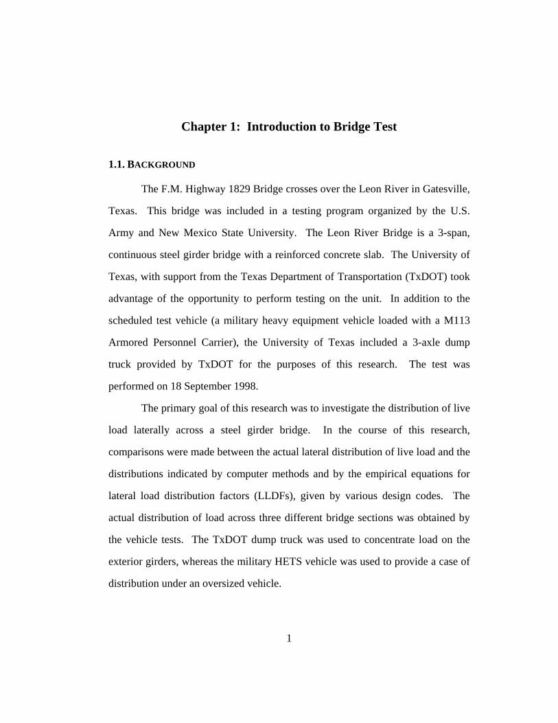
1.2. BRIDGE DESCRIPTION

The Leon River Bridge was erected in 1955. The bridge was designed

and built to fulfill H15-44 loading in accordance with the 1953 AASHTO

Standard Specifications. A profile of the center span of the bridge is shown in

Figure 1.1.

Figure 1.1: Profile View of Center Span of Leon River Bridge

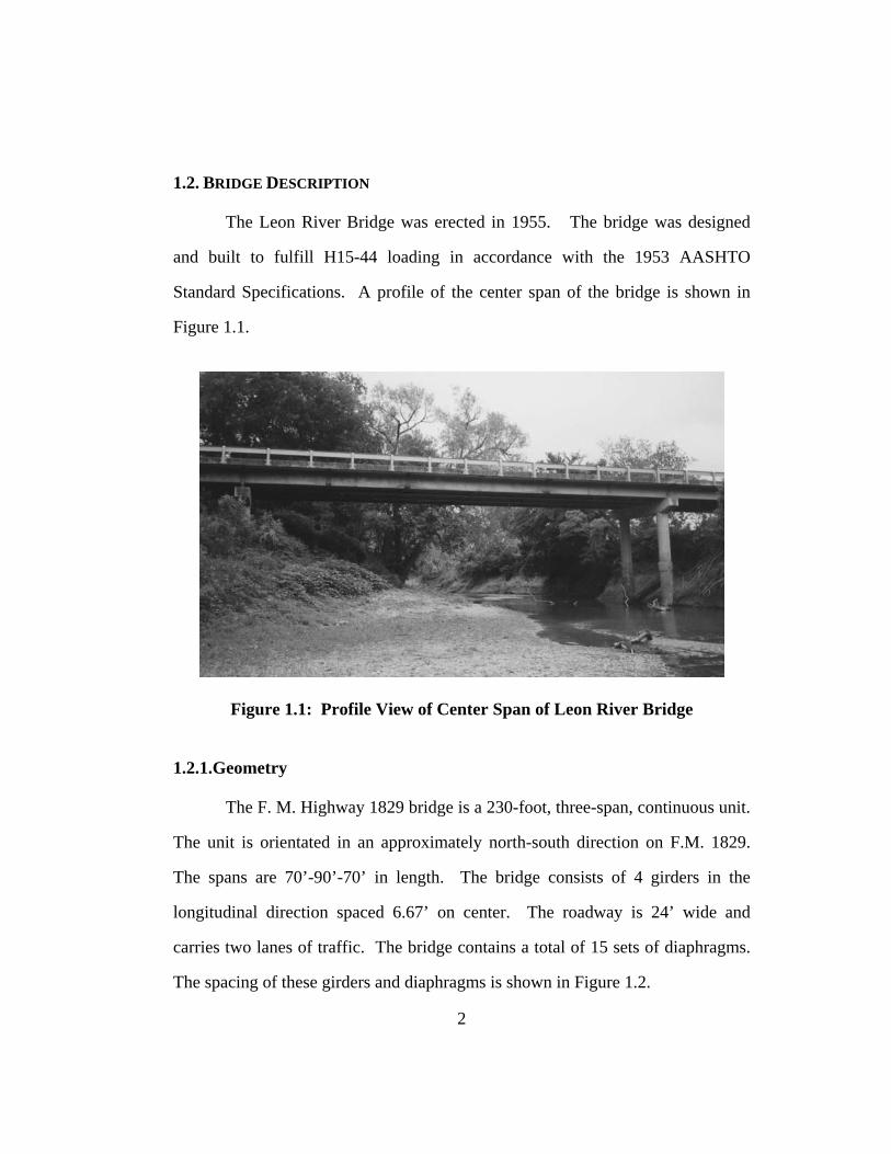
1.2.1.Geometry

The F. M. Highway 1829 bridge is a 230-foot, three-span, continuous unit.

The unit is orientated in an approximately north-south direction on F.M. 1829.

The spans are 70’-90’-70’ in length. The bridge consists of 4 girders in the

longitudinal direction spaced 6.67’ on center. The roadway is 24’ wide and

carries two lanes of traffic. The bridge contains a total of 15 sets of diaphragms.

The spacing of these girders and diaphragms is shown in Figure 1.2.

2

Diaphragms CL Girders

3 @ 6.67’" 25.67’

5 @ 15.0’ 20.0’ 19.375’"

CL Bridge CL Bearing

Figure 1.2: Plan View of Girder and Diaphragm Centerline Locations

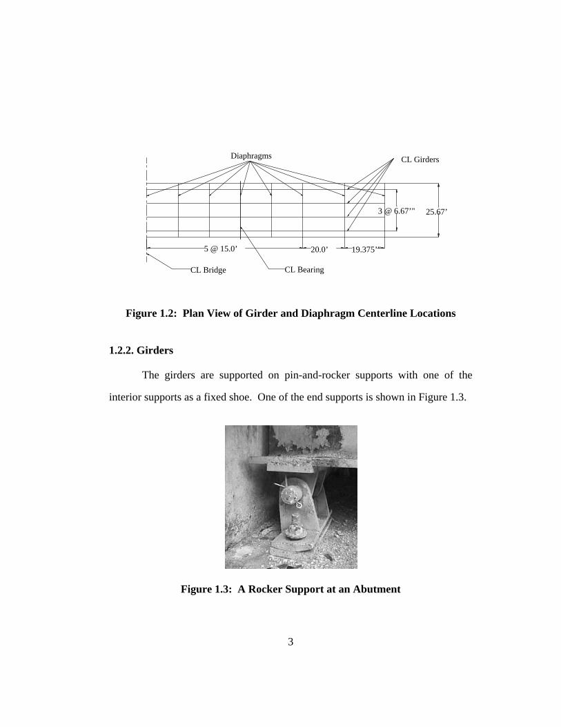
1.2.2. Girders

The girders are supported on pin-and-rocker supports with one of the

interior supports as a fixed shoe. One of the end supports is shown in Figure 1.3.

Figure 1.3: A Rocker Support at an Abutment

3

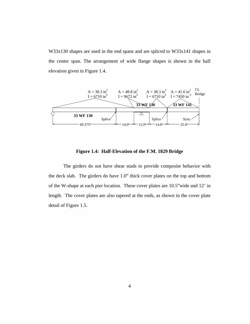
W33x130 shapes are used in the end spans and are spliced to W33x141 shapes in

the center span. The arrangement of wide flange shapes is shown in the half

elevation given in Figure 1.4.

14.0' 12.0' 14.0' 25.0'

A = 38.3 in2 I = 6710 in4

A = 38.3 in2 I = 6710 in4

A = 48.8 in2 I = 9672 in4

A = 41.6 in2 I = 7450 in 4

49.375'

33 WF 130

33 WF 130 33 WF 141

Splice Splice Sym.

CL Bridge

Figure 1.4: Half-Elevation of the F.M. 1829 Bridge

The girders do not have shear studs to provide composite behavior with

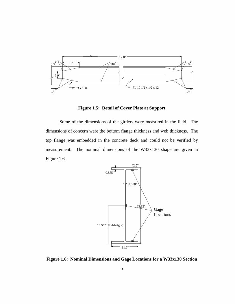
the deck slab. The girders do have 1.0” thick cover plates on the top and bottom

of the W-shape at each pier location. These cover plates are 10.5”wide and 12’ in

length. The cover plates are also tapered at the ends, as shown in the cover plate

detail of Figure 1.5.

4

1’

W 33 x 130 PL 10 1/2 x 1/2 x 12'

5.0"

12.0’

1/4

1/4

1/4

1/4

5/16

Figure 1.5: Detail of Cover Plate at Support

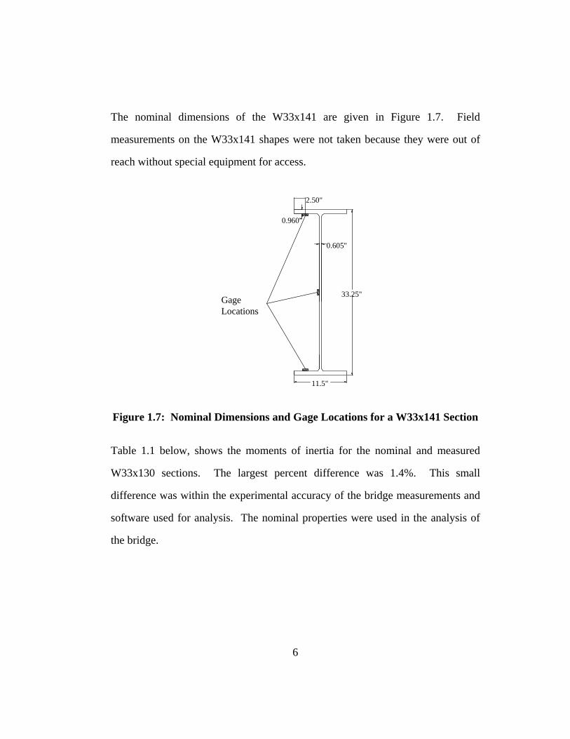
Some of the dimensions of the girders were measured in the field. The

dimensions of concern were the bottom flange thickness and web thickness. The

top flange was embedded in the concrete deck and could not be verified by

measurement. The nominal dimensions of the W33x130 shape are given in

Figure 1.6.

0.855"

33.12"

11.5"

0.580"

2.5"

16.56" (Mid-height)

Gage Locations

Figure 1.6: Nominal Dimensions and Gage Locations for a W33x130 Section

5

The nominal dimensions of the W33x141 are given in Figure 1.7. Field

measurements on the W33x141 shapes were not taken because they were out of

reach without special equipment for access.

0.605"

11.5"

33.25"

0.960"

2.50"

Gage Locations

Figure 1.7: Nominal Dimensions and Gage Locations for a W33x141 Section

Table 1.1 below, shows the moments of inertia for the nominal and measured

W33x130 sections. The largest percent difference was 1.4%. This small

difference was within the experimental accuracy of the bridge measurements and

software used for analysis. The nominal properties were used in the analysis of

the bridge.

6

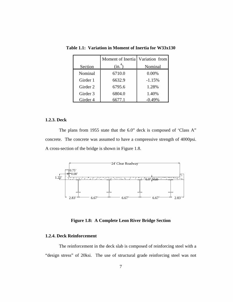
Table 1.1: Variation in Moment of Inertia for W33x130

Moment of Inertia Variation from

Section (in.4) NominalNominal 6710.0 0.00%Girder 1 6632.9 -1.15%Girder 2 6795.6 1.28%Girder 3 6804.0 1.40%Girder 4 6677.1 -0.49%

1.2.3. Deck

The plans from 1955 state that the 6.0” deck is composed of ‘Class A”

concrete. The concrete was assumed to have a compressive strength of 4000psi.

A cross-section of the bridge is shown in Figure 1.8.

1.25’ 0.08’

0.75’

2.83’ 6.67’ 6.67’ 6.67’ 2.83’

6.0" Slab

24' Clear Roadway

Figure 1.8: A Complete Leon River Bridge Section

1.2.4. Deck Reinforcement

The reinforcement in the deck slab is composed of reinforcing steel with a

“design stress” of 20ksi. The use of structural grade reinforcing steel was not

7

permitted. The typical mat consists of #5 bars spaced at 14”. Some extra #5 bars

are present at the curbs above every other diaphragm and are spaced at 7”. The

amount of reinforcement was assumed to be sufficient for the behavior considered

in this research.

1.2.5. Other Bridge Components

This section contains details about the other features of the Leon River

Bridge. These components include the railing, stiffeners, and diaphragms. The

assumed contribution of each to the bridge behavior is also presented here.

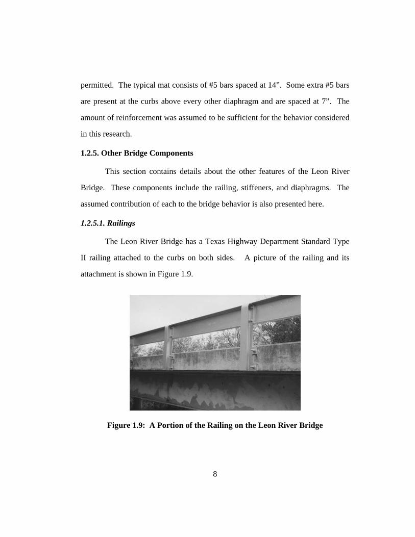
1.2.5.1. Railings

The Leon River Bridge has a Texas Highway Department Standard Type

II railing attached to the curbs on both sides. A picture of the railing and its

attachment is shown in Figure 1.9.

Figure 1.9: A Portion of the Railing on the Leon River Bridge

8

The four bolt connection at every location was assumed to not be rigid enough to

allow the railing to participate significantly in supporting moment. The railing

was not considered in any models or calculations done for the bridge.

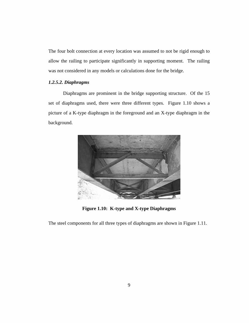
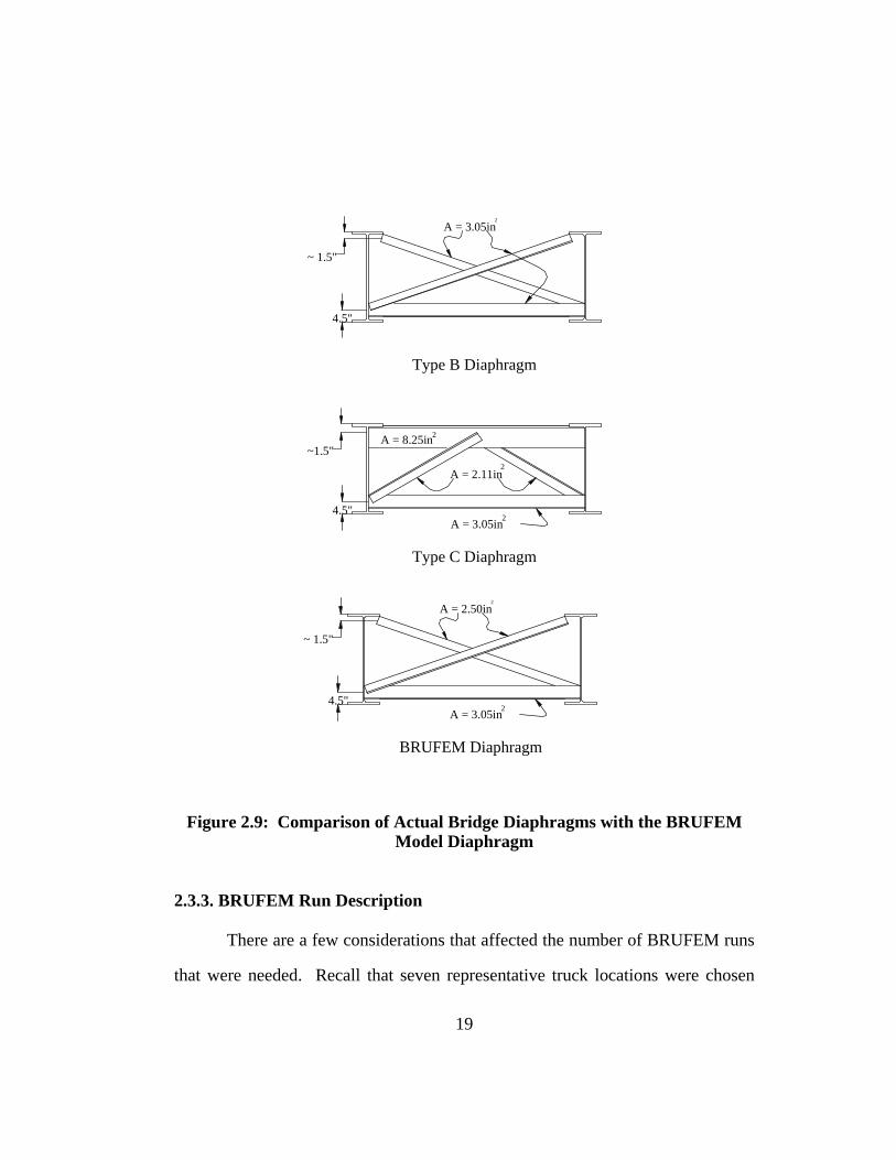
1.2.5.2. Diaphragms

Diaphragms are prominent in the bridge supporting structure. Of the 15

set of diaphragms used, there were three different types. Figure 1.10 shows a

picture of a K-type diaphragm in the foreground and an X-type diaphragm in the

background.

Figure 1.10: K-type and X-type Diaphragms

The steel components for all three types of diaphragms are shown in Figure 1.11.

9

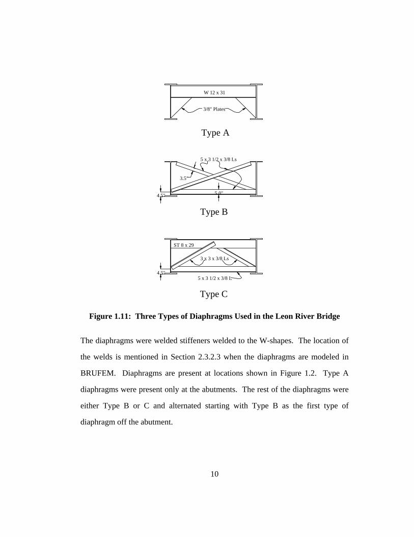
W 12 x 31

3/8" Plates

3.5"

5.0"

5 x 3 1/2 x 3/8 Ls

4.5"

4.5"5 x 3 1/2 x 3/8 L

3 x 3 x 3/8 Ls

ST 8 x 29

Type A

Type B

Type C

Figure 1.11: Three Types of Diaphragms Used in the Leon River Bridge

The diaphragms were welded stiffeners welded to the W-shapes. The location of

the welds is mentioned in Section 2.3.2.3 when the diaphragms are modeled in

BRUFEM. Diaphragms are present at locations shown in Figure 1.2. Type A

diaphragms were present only at the abutments. The rest of the diaphragms were

either Type B or C and alternated starting with Type B as the first type of

diaphragm off the abutment.

10

1.2.5.3. Stiffeners

Finally, web stiffeners were not used in the girders of the Leon River

Bridge. However, the curbs were considered as a stiffening element for the

exterior girders. The curbs contain approximately 81in2 of material and are

shown in Figure 1.8.

1.3. TEST INSTRUMENTATION AND DESCRIPTION

This section briefly describes the instrumentation and equipment used in

the Leon River Bridge test. The focus is on the strain gauges, the gauge locations,

and the load vehicles. Complete information on all the hardware and equipment

used can be found in Jauregui (1999).

1.3.1. Instrumentation and Equipment

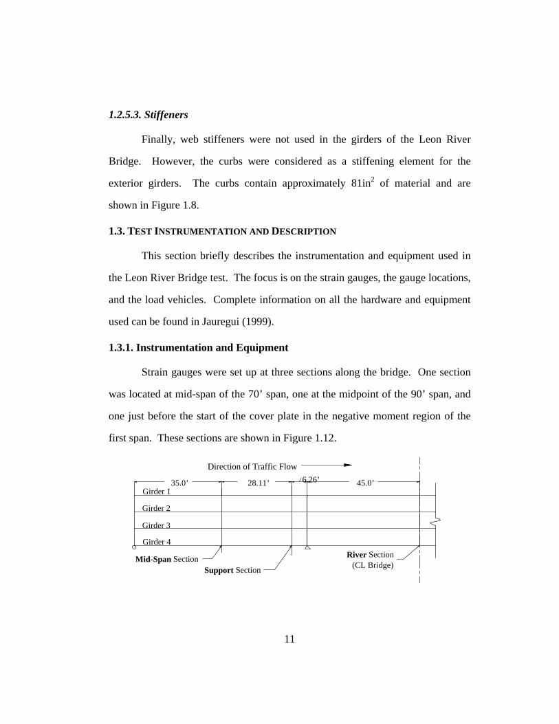
Strain gauges were set up at three sections along the bridge. One section

was located at mid-span of the 70’ span, one at the midpoint of the 90’ span, and

one just before the start of the cover plate in the negative moment region of the

first span. These sections are shown in Figure 1.12.

11

35.0’ 28.11’ 6.26’ 45.0’ Girder 1

Girder 2

Girder 3

Girder 4

Mid-Span Section Support Section

River Section (CL Bridge)

Direction of Traffic Flow

Figure 1.12: Location of Gauging Sections Used in Bridge Test

The terms “Mid-span”, “River” and “Support” appear in Figure 1.12 and

will be used throughout this research to refer to these sections. The River section

was so named because it was located at the mid-span of the 90’span over the Leon

River, and required special equipment for access. The sections for gauging were

chosen because they are locations of high positive and negative moment action.

The larger the strains measured, the smaller the error induced by the precision of

the data acquisition equipment.

1.3.1.1. The CR9000 and Related Equipment

A system of cables and junctions boxes was used in this test to carry the

signals from the strain gauges to the data acquisition software. The signals were

carried through a sequence that included the lead wires from the strain gauge, the

terminal block, completion box, junction box, the interior cards of the Campbell

Scientific CR9000C data logger, and the laptop computer. David V. Jauregui,

Ph.D, originally developed the equipment.

The CR9000C is the hardware that receives data from all the gauges. The

CR9000C has the capacity to receive data from eleven channels, each connected

to five strain gauges. In this test, only 38 gauges were used, requiring ten of the

eleven channels. Most channels did not have five active gauges. A more

complete description of the CR9000 can be found in Jauregui (1999).

The important characteristics of this system include the precision of the

data acquired and the sampling rate. The range of measurement for the gauges is

50mV. This was achieved with a noise level of ± 0.005mV (± 2με) for a ±

12

typical test run. A sampling rate of 10 Hz was used for low-speed tests. A rate of

100Hz was used for high-speed tests.

1.3.1.2. Gauges and Gauge Locations

The strain gauges used in this test are 10mm long. They were self-

temperature compensating. The lead wires were modified to fit the wiring

scheme required by the CR9000C hardware. The gauge factor for the steel

gauges was 2.11 and was acceptable for use in the range of temperatures

experienced during the instrumentation and testing (20-40oC). They were

mounted in accordance with manufacturer specifications.

The number and locations of gauges needs explanation. Three gauges

were placed at any given section, on any girder. One was located at mid-height

on the web one on the center of the top and bottom flanges on a given side. The

typical locations on the girder are shown in Figures 1.6 and 1.7. Three gauges

were used in this manner in order to accurately locate the neutral axis of the

girder-slab system, therefore indicating whether or not non-composite behavior

exists. All of the girders at a section were gauged in order to obtain the total

moment at that section. This total was checked with computer methods and was

used to yield the distribution of lateral load at the section, the major goal of this

research.

1.3.2. Load Vehicles

The Leon River Bridge was loaded with two different vehicles. The

lighter vehicle was 3-axle TxDOT dump truck. A picture of the dump truck is

shown below.

13

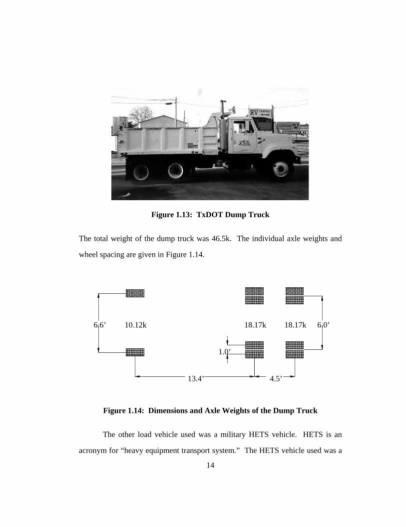
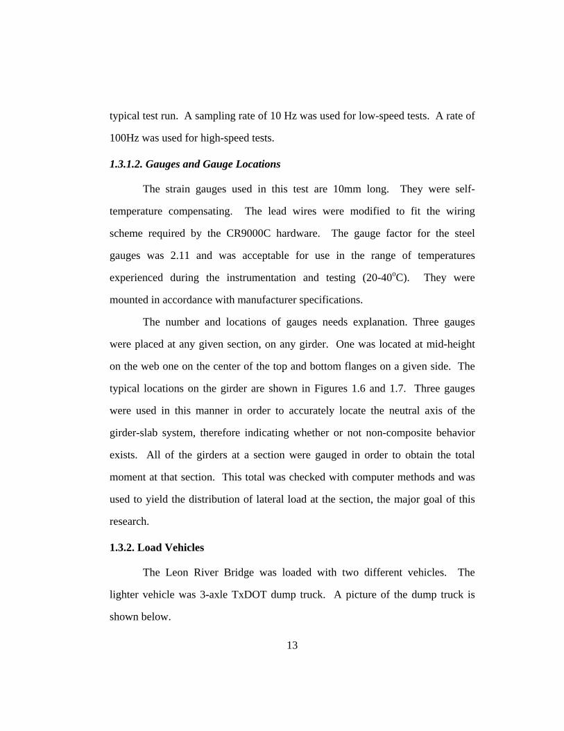
Figure 1.13: TxDOT Dump Truck

The total weight of the dump truck was 46.5k. The individual axle weights and

wheel spacing are given in Figure 1.14.

6.6’

13.4’ 4.5’

1.0’

10.12k 18.17k 18.17k 6.0’

Figure 1.14: Dimensions and Axle Weights of the Dump Truck

The other load vehicle used was a military HETS vehicle. HETS is an

acronym for “heavy equipment transport system.” The HETS vehicle used was a

14

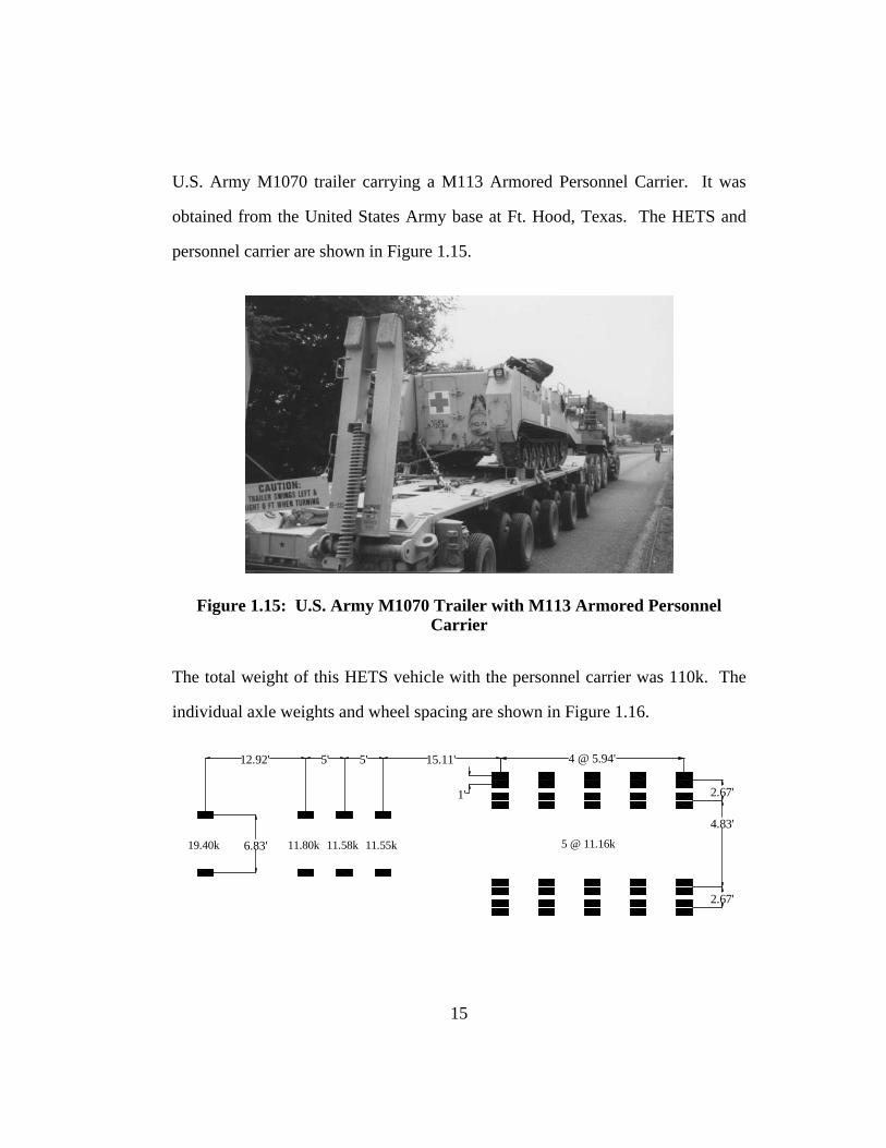
U.S. Army M1070 trailer carrying a M113 Armored Personnel Carrier. It was

obtained from the United States Army base at Ft. Hood, Texas. The HETS and

personnel carrier are shown in Figure 1.15.

Figure 1.15: U.S. Army M1070 Trailer with M113 Armored Personnel Carrier

The total weight of this HETS vehicle with the personnel carrier was 110k. The

individual axle weights and wheel spacing are shown in Figure 1.16.

15

19.40k 11.80k 11.58k 11.55k 5 @ 11.16k

1'

6.83'

12.92' 5' 5' 15.11'

2.67'

4.83'

2.67'

4 @ 5.94'

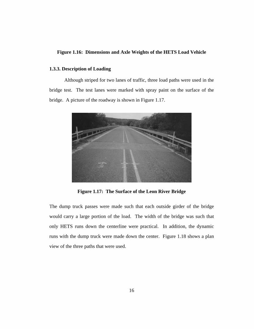
Figure 1.16: Dimensions and Axle Weights of the HETS Load Vehicle

1.3.3. Description of Loading

Although striped for two lanes of traffic, three load paths were used in the

bridge test. The test lanes were marked with spray paint on the surface of the

bridge. A picture of the roadway is shown in Figure 1.17.

Figure 1.17: The Surface of the Leon River Bridge

The dump truck passes were made such that each outside girder of the bridge

would carry a large portion of the load. The width of the bridge was such that

only HETS runs down the centerline were practical. In addition, the dynamic

runs with the dump truck were made down the center. Figure 1.18 shows a plan

view of the three paths that were used.

16

Double Yellow Lines

HETS Left Wheel Path

Left Wheel, Path 3-4Right Wheel, Path 1-2

24' Roadway

10" Curbs

11.33’

11.33’ 8.5’

20' (typ.)

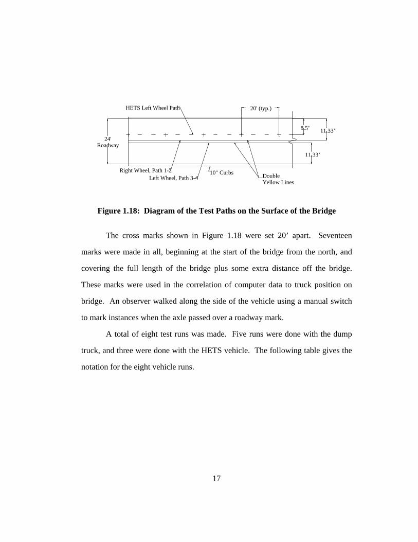
Figure 1.18: Diagram of the Test Paths on the Surface of the Bridge

The cross marks shown in Figure 1.18 were set 20’ apart. Seventeen

marks were made in all, beginning at the start of the bridge from the north, and

covering the full length of the bridge plus some extra distance off the bridge.

These marks were used in the correlation of computer data to truck position on

bridge. An observer walked along the side of the vehicle using a manual switch

to mark instances when the axle passed over a roadway mark.

A total of eight test runs was made. Five runs were done with the dump

truck, and three were done with the HETS vehicle. The following table gives the

notation for the eight vehicle runs.

17

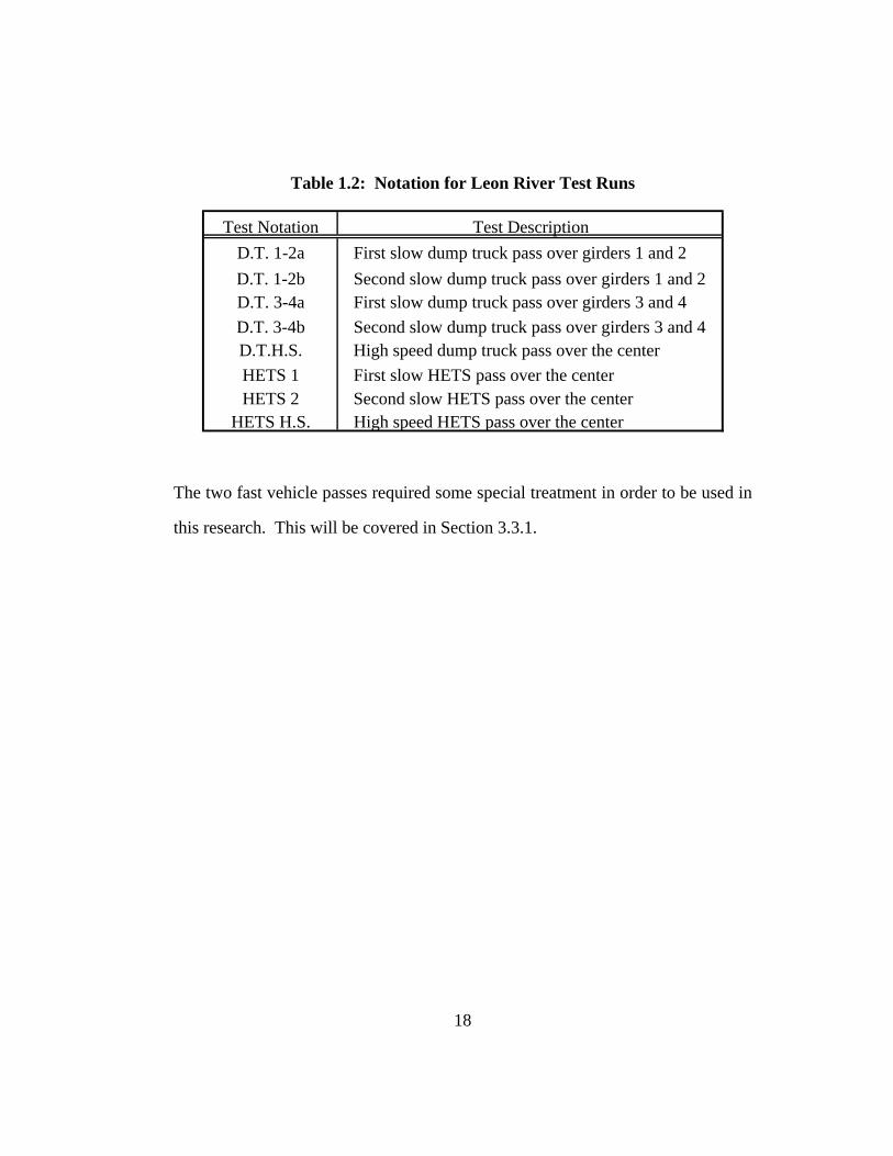
Table 1.2: Notation for Leon River Test Runs

Test Notation Test DescriptionD.T. 1-2a First slow dump truck pass over girders 1 and 2D.T. 1-2b Second slow dump truck pass over girders 1 and 2D.T. 3-4a First slow dump truck pass over girders 3 and 4D.T. 3-4b Second slow dump truck pass over girders 3 and 4D.T.H.S. High speed dump truck pass over the centerHETS 1 First slow HETS pass over the centerHETS 2 Second slow HETS pass over the center

HETS H.S. High speed HETS pass over the center

The two fast vehicle passes required some special treatment in order to be used in

this research. This will be covered in Section 3.3.1.

18

Chapter 2: Computer Analysis Methods

2.1. OVERVIEW OF TWO TYPES OF ANALYSIS METHODS

Computer programs were used to predict moments and stresses produced

in the field by the test vehicles. The estimated stresses were compared to the

measured stresses in order to determine whether or not the computer analysis gave

viable results. An accurate, sophisticated method of computer analysis allows

designers to design structures safely and with greater accuracy than design

equations. The major computer package used in this research was BRUFEM

(Bridge Rating Using Finite Element Methods) developed by the Florida

Department of Transportation (FDOT). SAP2000 Nonlinear, a commercially

available program, was also used. BRUFEM was used to generate lateral load

distribution factors (LLDFs). SAP2000 was used to help reduce the data from the

field tests.

2.2. ANALYSIS USING SAP2000

The SAP2000 software was used to perform a series of line girder

analyses. A line girder analysis is a one-dimensional analysis used to obtain the

total static moment present in a specific cross-section of the bridge for any

position of a load vehicle. This was accomplished through a series of steps. First

of all, a model of one girder was made in SAP2000. Then the influence lines for

each gauged section were generated. These influence lines were then used to

generate moment histories for each section under the action of each load vehicle.

A complete history of the total flexural moment at a given cross-section was

1

plotted as a function of vehicle position. This information was useful because it

determined the vehicle positions in which the total flexural moment at a cross-

section was a maximum, minimum, or other significant value.

A full description of the procedure for a line girder analysis using

SAP2000 Nonlinear can be found in Appendix A of McIlrath (1994). A computer

package other than SAP2000 can be used, as long as it has the ability to generate

influence lines. This section first outlines the element types, boundary conditions,

and model details used in the SAP2000 line girder model of the Leon River

Bridge. Then the method of obtaining the moment histories from the line girder

model is covered.

2.2.1. SAP2000 Nonlinear Model Specifics

The first step in the line girder analysis was to model the properties of a

single girder in SAP2000. The model included all the proper support conditions

and section properties. Many properties for standard W shapes are automatically

included in SAP2000. The section with the cover plates was user-defined and

only required the cross-sectional area (48.8 in2) and the moment of inertia about

the primary bending axis (9672 in4). Figure 1.4 in the previous chapter shows a

half-elevation of the Leon River Bridge girder with the properties used for the

SAP2000 model.

A girder with three spans (70’-90’-70’) was modeled with three-

dimensional frame elements. Nodes were used to divide the girder into segments.

A node was placed at every change in geometry of the girder, every support

location, and at every location corresponding with one of the three gauged

2

sections. Each segment created was divided with additional “output” nodes to

give additional refinement to the model. The SAP2000 model used contained 14

joints, 13 basic frame segments, and 5,483 output segments. The output nodes

were spaced such that the average length of any output segment was 0.0417 feet.

The travel lane and load vehicles needed to be defined in order to run the

model. With this one-dimensional model, only one lane assignment existed. The

lane was defined as the centerline of the line girder, moving from left to right.

The load vehicles were defined in SAP2000 to check the model for errors by

correlating moments generated in SAP2000 with those generated by other

analysis software. Load vehicles were defined as single wheels spaced at the

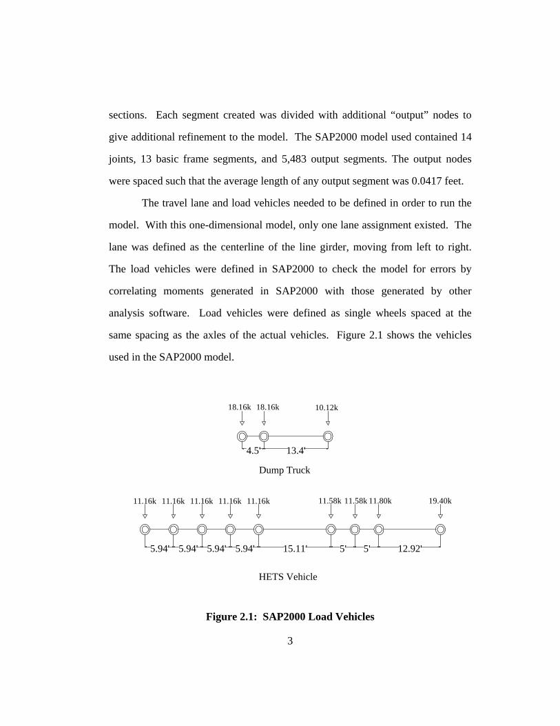
same spacing as the axles of the actual vehicles. Figure 2.1 shows the vehicles

used in the SAP2000 model.

11.16k 11.16k 11.16k 11.16k 11.16k 11.58k 11.58k 11.80k 19.40k

5.94' 5.94' 5.94' 5.94' 15.11' 5' 5' 12.92'

4.5' 13.4'

10.12k18.16k 18.16k

Dump Truck

HETS Vehicle

Figure 2.1: SAP2000 Load Vehicles

3

Notice that each wheel in the SAP2000 load vehicle was given the load of the

entire axle of the real load vehicle. This was necessary in order calculate total

moment due to the whole vehicle, which was used in calculating LLDFs.

2.2.2. Using a Spreadsheet to Generate Moment Histories

SAP2000 was used to generate moment influence lines for three points on

the line girder that correspond to Mid-span, Support, and River sections on the

bridge. The influence line values indicate the moment generated at the location of

interest, from a unit load at any location along the girder. Using this concept, a

spreadsheet program was used to generate the required flexural moment histories.

The spacing of the axles and the total axle weights were required to use

this method. These were given in Figure 2.1. The resulting influence line values

were tabulated at increments small enough that the amount of interpolation was

minimized. The influence line increments in SAP2000 were 0.0417 ft. (0.5 in.).

This high level of refinement was used because most of the axle spacings are

evenly divisible by 0.5in.

Once defined, the axle weights were moved incrementally in the

spreadsheet representing the path of the load vehicle. At each increment, the

weight on the axle was multiplied by the influence line value to give a value of

moment for that axle location. The effects of all the axles were summed up to get

a moment value for the vehicle position. In the event that an axle did not line up

with an influence line value, an average of the two closest values was used. This

was acceptable because of the small length of output segments used in this

method. The history of moment versus vehicle position was developed in this

4

manner. This method worked well as long as the user kept track of which axles

are on or off the girder.

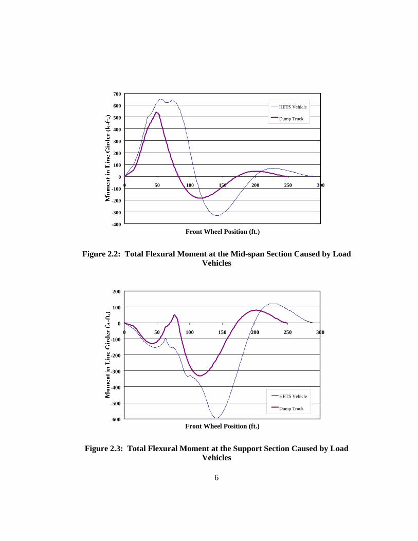
2.2.3. Presentation of Moment Histories

A line girder analysis was performed using the 3-axle dump truck as well

as the 9-axle HETS vehicle. The total length, axle-to-axle, of the HETS vehicle

was longer than the dump truck (61.7’ compared to 17.9’). Therefore the method

needed to be carried out until the front axle of the HETS was 290ft from the

beginning of the bridge. At that point the rearmost axle was almost off the bridge

and the moments generated were close to zero. The front axle of the dump truck

only needed to be moved to 249ft from the beginning of the bridge to complete

the traverse of the bridge. The moment histories for each section considering both

vehicles are shown in the following figures.

5

-400

-300

-200

-100

0

100

200

300

400

500

600

700

0 50 100 150 200 250 300

Front Wheel Position (ft.)

HETS Vehicle

Dump Truck

Figure 2.2: Total Flexural Moment at the Mid-span Section Caused by Load Vehicles

-600

-500

-400

-300

-200

-100

0

100

200

0 50 100 150 200 250 300

Front Wheel Position (ft.)

HETS Vehicle

Dump Truck

Figure 2.3: Total Flexural Moment at the Support Section Caused by Load Vehicles

6

-200

-100

0

100

200

300

400

500

600

700

800

900

0 50 100 150 200 250 300

Front Wheel Position (ft.)

HETS Vehicle

Dump Truck

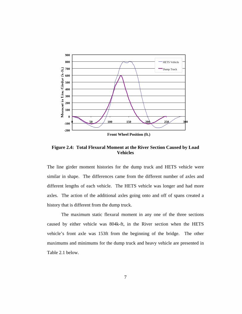
Figure 2.4: Total Flexural Moment at the River Section Caused by Load Vehicles

The line girder moment histories for the dump truck and HETS vehicle were

similar in shape. The differences came from the different number of axles and

different lengths of each vehicle. The HETS vehicle was longer and had more

axles. The action of the additional axles going onto and off of spans created a

history that is different from the dump truck.

The maximum static flexural moment in any one of the three sections

caused by either vehicle was 804k-ft, in the River section when the HETS

vehicle’s front axle was 153ft from the beginning of the bridge. The other

maximums and minimums for the dump truck and heavy vehicle are presented in

Table 2.1 below.

7

Table 2.1: Maximum Line Girder Moments in the Leon River Bridge

Maximum Maximum Vehicle FrontPositive/Negative Moment Axle Location

Vehicle Moments (k-ft.) Sections at Maximum (ft.)Dump Truck 593 River 129

-331 Support 116HETS 804 River 153

-596 Support 141

Notice that neither of the maximum moment effects comes from the Mid-span

section.

2.2.4. Truck Positions of Interest

Before the test data was reduced, the distribution of moment in the bridge

was not known. It was expected that the vehicle position that gives the largest

value of moment over a section might also give the largest value of moment

experienced by any one girder. This was not a certainty. Table 2.2 contains the 7

different vehicle positions that were analyzed in detail in this research. The

reasoning for selecting each vehicle position is also given in the table. For

example, the front axle position of 57’ was picked because it is at this location

that the HETS causes the maximum positive moment in the Mid-span section.

Some other positions were chosen expecting a maximum negative value.

Originally, 10 values were chosen, including 3 locations where zero moment was

expected. Locations at 80’, 174’, and 200’ were discarded because of the

numerical instability of the near-zero moment values.

8

Table 2.2: Representative Vehicle Positions Selected From Line Girder Analysis

Vehicle Front Vehicle CausingWheel Position (ft.) Effect

50 Dump Truck57 HETS

107 -120 Dump Truck129 Dump Truck139 HETS155 HETS

River Positive Moment Maximum Support Negative Moment Maximum River Positive Moment Maximum Support Negative Moment Maximum River Positive Moment

Significant Effect Maximum Mid-span Positive Moment Maximum Mid-span Positive Moment

2.3. ANALYSIS PROCEDURE USING BRUFEM

In addition to line girder analyses from SAP2000, a three-dimensional

finite element analysis was performed using BRUFEM. BRUFEM was

developed by FDOT for use in analysis, rating and design of highway bridges.

BRUFEM version 4.20 revised 30 August 1996 was used in this research. The

package contains modeling capabilities that are tailored to various bridge types.

The steel bridge modeling method was used in this research.

The BRUFEM software is contained in four FORTRAN programs,

BRUFEM1, SIMPAL, BRUFEM3, and SMPLOT. The most important files used

or generated by these programs are the HISTORY. PRE, BAR.DAT, VEH.DAT,

and the BRATE.OUT file. These files will be mentioned in subsequent sections

of this chapter in order to describe the BRUFEM model. BRUFEM1 creates the

finite element model using interactive input from the user as well as prepared

input files. The user-prepared BAR.DAT file contains the properties of the steel

girders, and the user-prepared VEH.DAT files contain the description of the load

9

vehicles. SIMPAL performs the finite element analysis and generates the output

files and data files used in plotting. The actual bridge rating is performed by

BRUFEM3. This program generates the LLDFs contained in a file named

BRATE.OUT. The fourth program is SIMPLOT, which is used for plotting

analysis results in a graphics environment. SIMPLOT was not used extensively

in this research. More information on the BRUFEM package can be found in the

BRUFEM manual by Hays (1994).

A major output of the BRUFEM package is lateral load distribution

factors. These factors were generated for the three sections of the Leon River

Bridge. They were compared with the distribution factors obtained from the test

data. This comparison gave insight into how well the package works, and the

usefulness of the package over accepted design equations.

2.3.1. Types of BRUFEM Analyses for Steel Girder Bridges

The basic BRUFEM model for a steel bridge contains the bridge girders

and a deck slab. Additional elements such as parapets, diaphragms, and railings

can be added to the basic model. The BRUFEM package can model a bridge

system either compositely or non-compositely. For non-composite action, the

girder and slab elements act independently, and the centroid of the girder and slab

coincide. The slab only undergoes plate bending and acts primarily to distribute

the wheel loads to the girders. In modeling for composite action, the girder-slab

interaction can be modeled one of two ways. The first method is the Composite

Girder Model (CGM) and the second is the Eccentric Girder Model (ECM). A

short comparison of the results from both methods is given in Chapter 5.

10

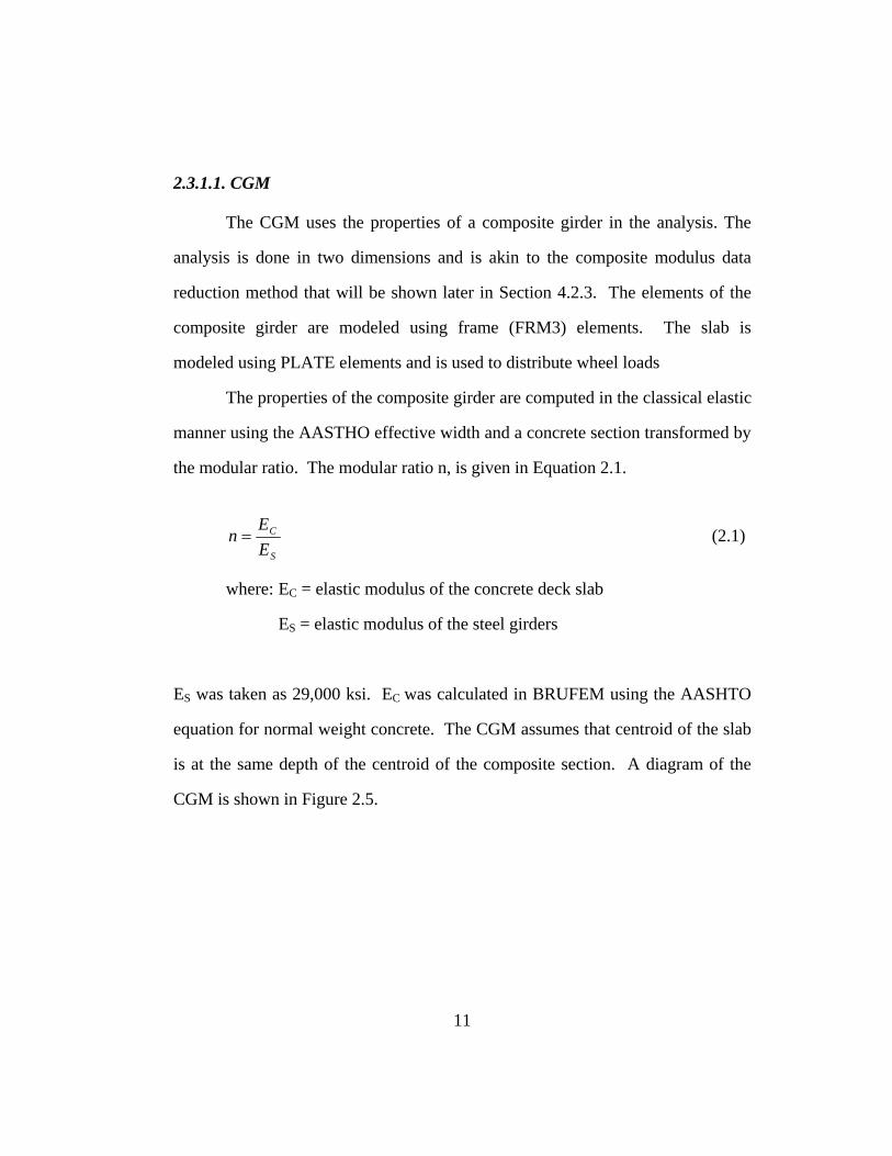
2.3.1.1. CGM

The CGM uses the properties of a composite girder in the analysis. The

analysis is done in two dimensions and is akin to the composite modulus data

reduction method that will be shown later in Section 4.2.3. The elements of the

composite girder are modeled using frame (FRM3) elements. The slab is

modeled using PLATE elements and is used to distribute wheel loads

The properties of the composite girder are computed in the classical elastic

manner using the AASTHO effective width and a concrete section transformed by

the modular ratio. The modular ratio n, is given in Equation 2.1.

S

C

EE

n = (2.1)

where: EC = elastic modulus of the concrete deck slab

ES = elastic modulus of the steel girders

ES was taken as 29,000 ksi. EC was calculated in BRUFEM using the AASHTO

equation for normal weight concrete. The CGM assumes that centroid of the slab

is at the same depth of the centroid of the composite section. A diagram of the

CGM is shown in Figure 2.5.

11

eff

eff / n

b

b

Slab Elements(Plate Bending)

Centroid ofComposite

Section

Figure 2.5: Modeling Composite Action Using the BRUFEM Composite Girder Model

In BRUFEM, the effective width of the concrete slab is also calculated using

AASHTO recommendations.

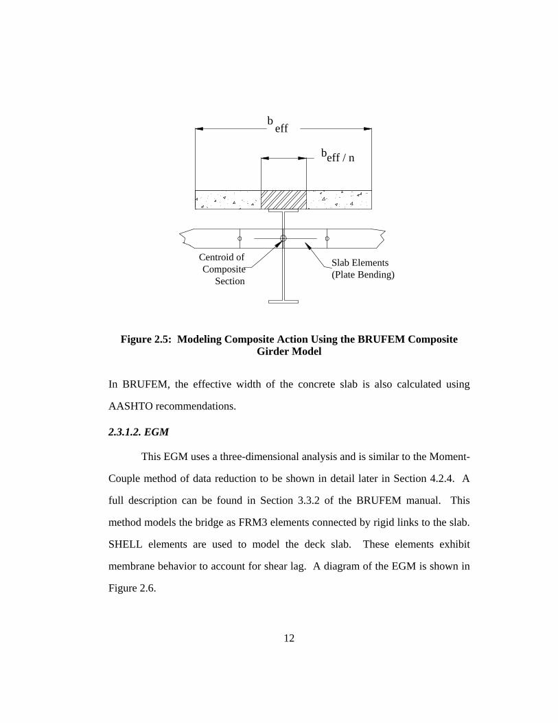
2.3.1.2. EGM

This EGM uses a three-dimensional analysis and is similar to the Moment-

Couple method of data reduction to be shown in detail later in Section 4.2.4. A

full description can be found in Section 3.3.2 of the BRUFEM manual. This

method models the bridge as FRM3 elements connected by rigid links to the slab.

SHELL elements are used to model the deck slab. These elements exhibit

membrane behavior to account for shear lag. A diagram of the EGM is shown in

Figure 2.6.

12

e

Centroid of Girder Alone

Shell Elements (Plate Bending and Plane Stress)

Rigid Link

Figure 2.6: Modeling Composite Action Using the BRUFEM Eccentric Girder Model

According to the BRUFEM manual, the EGM is considered to be the more

precise method as long as a sufficient number of elements are used in the

longitudinal direction to attain strain compatibility between the girder and slab.

2.3.1.3. Modeling Diaphragms

In a study done during the development of BRUFEM, BRUFEM models

containing diaphragms were considered slightly stiffer than other three-

dimensional models without diaphragms. BRUFEM also only models X-type or

steel beam type diaphragms. Appendix I of the BRUFEM manual gives a study

on the effects of modeling using X-type diaphragms instead of K-type

diaphragms. These two results indicate that in some cases, the BRUFEM models

will underestimate the maximum girder moments and shears. BRUFEM corrects

this in the post processor by increasing the live load moments and shears by 5%.

13

Since this underestimation is slight in most cases, this 5% was removed from the

BRUFEM results for this research.

2.3.2. Leon River Model

The primary purpose of this research was to explore moment distribution

in the Leon River Bridge using the results of a BRUFEM model. In order to

accomplish this goal, some simplifications in the Leon River Bridge model were

made. All of the basic model parameters entered by the user for the bridge are

found in the HISTORY.PRE files that are reprinted in Appendix A. This section

will give an overview of the BRUFEM model that was used.

2.3.2.1. Geometry

A few simplifications were made to the bridge model for use in the

BRUFEM system. The nominal span lengths are 70’-90’-70’. The centerlines of

the supports at the abutments are located 0.625’ from the end, which gives and

actual end span length of 69.375’. The nominal span length of 70’ was used in

this analysis.

The finite element model used 1840 slab elements, and 460 beam

elements. Each girder was subdivided in 115 elements. The two 70’ spans each

contained 35 elements in the longitudinal direction. The 90’ interior span

contained 45 elements. The recommended number of elements per span

according to the BRUFEM manual is 20 in the longitudinal direction. The deck

slab contained 16 elements in the lateral direction and 115 elements in the

longitudinal direction. The typical slab element used was 2’ x 1.67’.

14

BRUFEM models steel girders as built-up sections using FRM3 frame

elements. The fillets in girders were ignored. The flange and web widths and

depths for each W section were used to define the girders. The cover plates were

treated as 10.5” x 0.5” x 12’-0” rectangles. The tapering of the cover plate at the

ends was ignored. The BAR.DAT file contains the geometry of the steel girder

and can be found in Appendix A.

BRUFEM allows for modeling deck material that extends beyond the

centerlines of the exterior girders. A slab width of 2.83’ was used in this analysis.

The additional 81in2 of concrete that comprises the curbs was not included in the

model. The guardrails were also not modeled in BRUFEM.

2.3.2.2. Load Vehicles

The wheel configuration of the HETS vehicle could not be modeled

exactly in BRUFEM. The axles of BRUFEM load vehicles are defined using

representative distances on the axle. A schematic of a typical spacing is shown in

Figure 2.7(a).

15

W1

W

W1W2

W1

Load per wheel = 2.79k

W = 2.67' G = 4.83'

W1 = 1' W2 = 1.67'

G

G

(c)

(b)

W

W1W2

WWW

Load per wheel = 1.395 k

G

(a)W

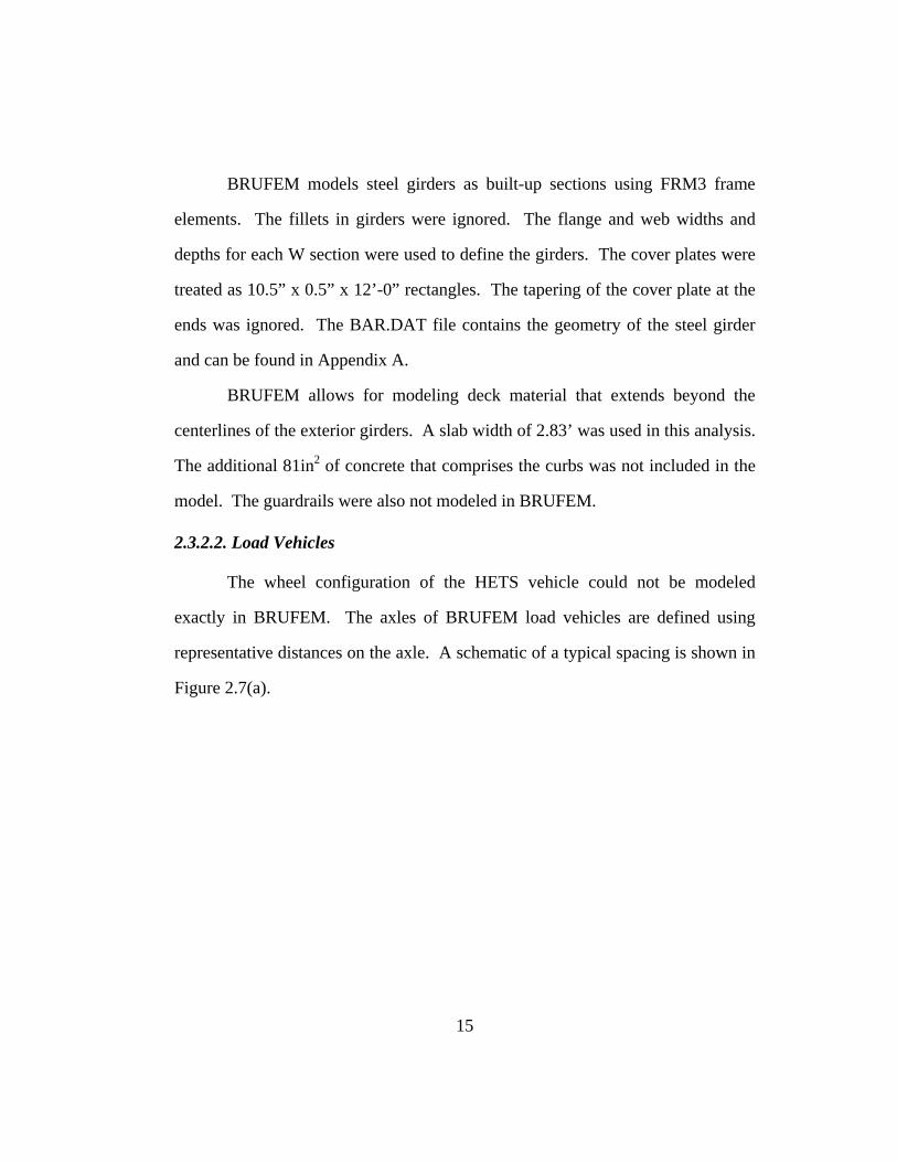
Figure 2.7: Typical Axle Modeling using BRUFEM

The gauge, G, is the distance between the two innermost wheels. The spacing

between any of the wheels outside of the innermost two is given by W. In

BRUFEM, W must be the same for all wheels on an axle. Figure 2.7(b) shows

one the HETS axles. The spacings of all the wheels on the HETS axle are not the

same. Some of the wheels on the HETS axle are spaced at 1.67’, where others are

spaced at 1’. The solution to this conflict was modeling each pair of wheels one

foot apart as a single wheel, with double the load (Figure 2.7(c)). The full HETS

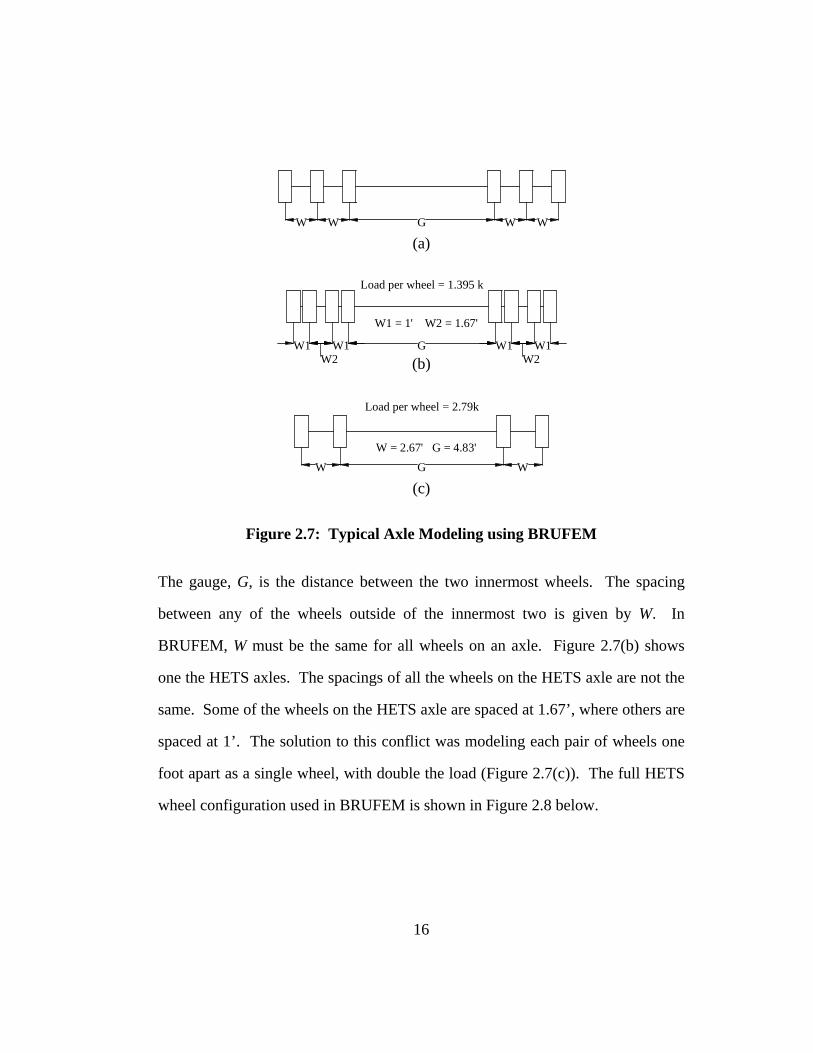
wheel configuration used in BRUFEM is shown in Figure 2.8 below.

16

19.40k 11.58 k11.80 k 11.55 k 5 @ 11.16k

12.92' 5' 5' 15.11' 4 @ 5.94'

2.67'

4.83'

2.67'

Figure 2.8: Modified HETS Wheel Pattern for BRUFEM Modeling

The differences between the model HETS vehicle and the actual vehicle are

subtle. The resolution of the finite element mesh is 1.67’ in the lateral direction

so modeling two loads spaced at 1’ as one load was not crucial. This HETS and

the dump truck modeling information are contained in the user-prepared

VEH.DAT files that can be found in Appendix A.

2.3.2.3. Diaphragms

The results of Section 5.3.2 of this research conclude that diaphragms

need to be included in the BRUFEM model. Section 1.2.5 contained the details

regarding the three different types of diaphragms that exist in the Leon River

Bridge. The bridge contains X-type, K-type, and steel beam type diaphragms.

The BRUFEM model includes default diaphragms at support locations. These

default diaphragms are 8 in. wide and are 80% as deep as the girder section. This

17

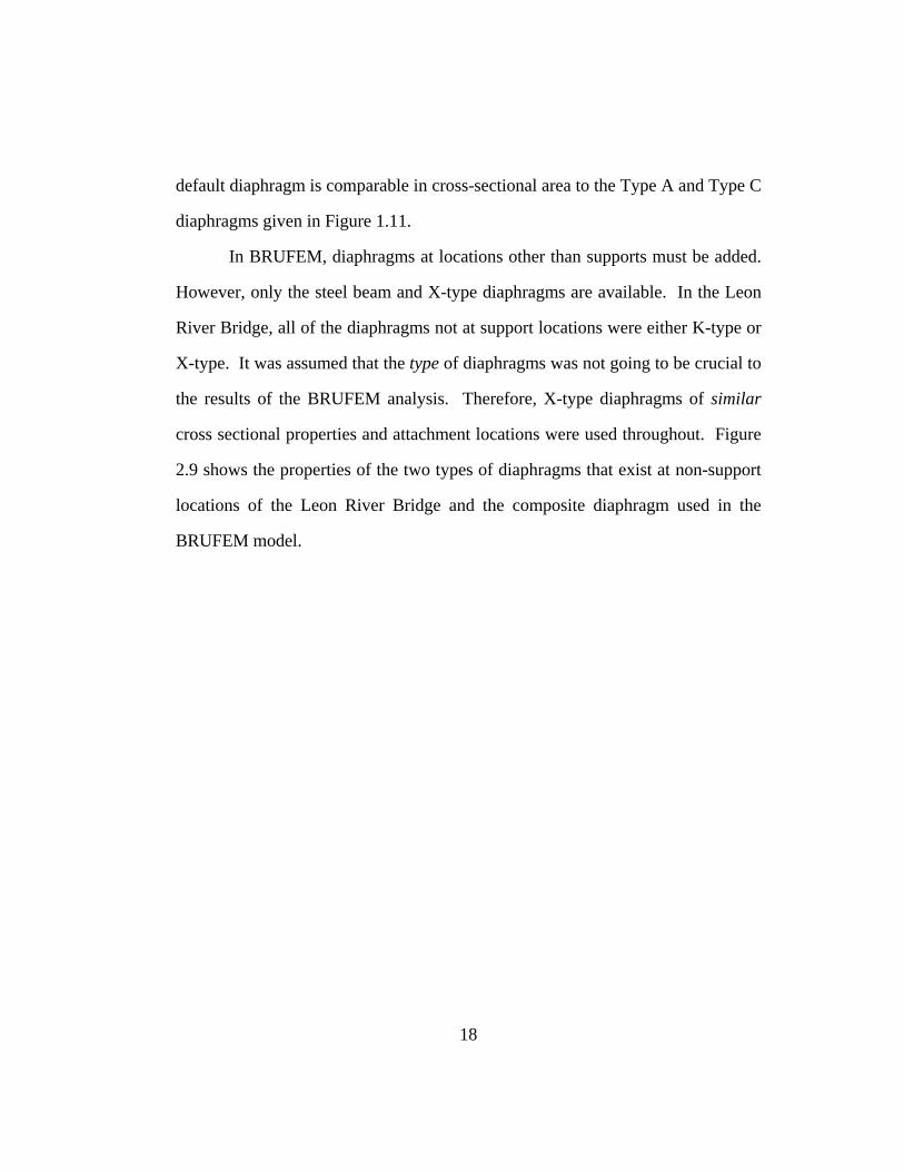
default diaphragm is comparable in cross-sectional area to the Type A and Type C

diaphragms given in Figure 1.11.

In BRUFEM, diaphragms at locations other than supports must be added.

However, only the steel beam and X-type diaphragms are available. In the Leon

River Bridge, all of the diaphragms not at support locations were either K-type or

X-type. It was assumed that the type of diaphragms was not going to be crucial to

the results of the BRUFEM analysis. Therefore, X-type diaphragms of similar

cross sectional properties and attachment locations were used throughout. Figure

2.9 shows the properties of the two types of diaphragms that exist at non-support

locations of the Leon River Bridge and the composite diaphragm used in the

BRUFEM model.

18

~ 1.5"

4.5"

Type B Diaphragm

A = 3.05in2

~1.5"

4.5"

Type C Diaphragm

A = 3.05in

A = 2.11in

2 A = 8.25in

2

2

~ 1.5"

4.5"

BRUFEM Diaphragm

A = 3.05in2

A = 2.50in2

Figure 2.9: Comparison of Actual Bridge Diaphragms with the BRUFEM Model Diaphragm

2.3.3. BRUFEM Run Description

There are a few considerations that affected the number of BRUFEM runs

that were needed. Recall that seven representative truck locations were chosen

19

20

for analysis of moment distribution. In a single BRUFEM analysis, a load

vehicle can be moved to all of these locations. Recall from Figure 1.18 that the

two dump truck lanes were symmetric about the bridge’s longitudinal centerline.

Therefore, only one of the dump truck’s lateral positions needed to be modeled.

Thus, with only two BRUFEM analyses, one for the HETS and one for the dump

truck, a full set of data for comparison was acquired.

For completeness, two BRUFEM runs were made using the CGM and two

were made using the EGM method (one for each test vehicle). Since the ECM

more accurately represents what is potentially happening in the slab-girder

interaction, that method was chosen to investigate the behavior of the diaphragms

and their role in the distribution of moment across the girders. A set of runs using

the ECM was performed with the diaphragms removed in order to judge their

importance to the model.

In summary, one run using the CGM, one using the ECM with diaphragms

and one using the ECM without diaphragms was made for each vehicle. There

were three major files that describe each run. These were the HISTORY.PRE,

BAR.DAT, and VEH.DAT files. All essential BRUFEM files are included in

Appendix A.

Chapter 3: Initial Test Results and Data Reduction

This chapter contains an explanation of the initial data reduction

performed on the strains measured during the Leon River Bridge test. It also

discusses some of the steps taken to put the initial strain data in usable format for

the calculation of moments. The gauging scheme allowed for the calculation of

moment in every girder of the bridge. The moment distribution factors were then

computed using all the individual girder moments.

The initial data reduction problem was to determine the flexural

participation of the slab with the girders. The bridge was designed non-

compositely. The location of the neutral axis (N.A.) for a girder cross-section was

used to determine the degree of composite action of the system.

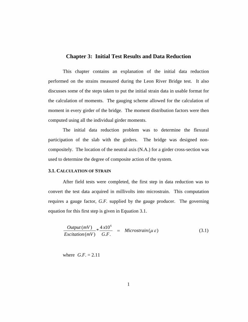
3.1. CALCULATION OF STRAIN

After field tests were completed, the first step in data reduction was to

convert the test data acquired in millivolts into microstrain. This computation

requires a gauge factor, G.F. supplied by the gauge producer. The governing

equation for this first step is given in Equation 3.1.

)(..

104*)(

)( 6

εμnMicrostraiFG

xmVExcitation

mVOutput= (3.1)

where G.F. = 2.11

1

The power for the system is a 12V battery, which is stepped down in order to

provide a 5V excitation to the gauge system The excitation voltage was

approximately 5,000 mV for all the tests. Typical output voltages for extreme

strains were between –0.26 and 0.45 mV for the dump truck tests. This gave

typical extreme strains between –150 and 200με. The output and input excitation

voltage were provided in the data acquired by the computer. A spreadsheet was

used to convert millivolts into microstrain for all test runs.

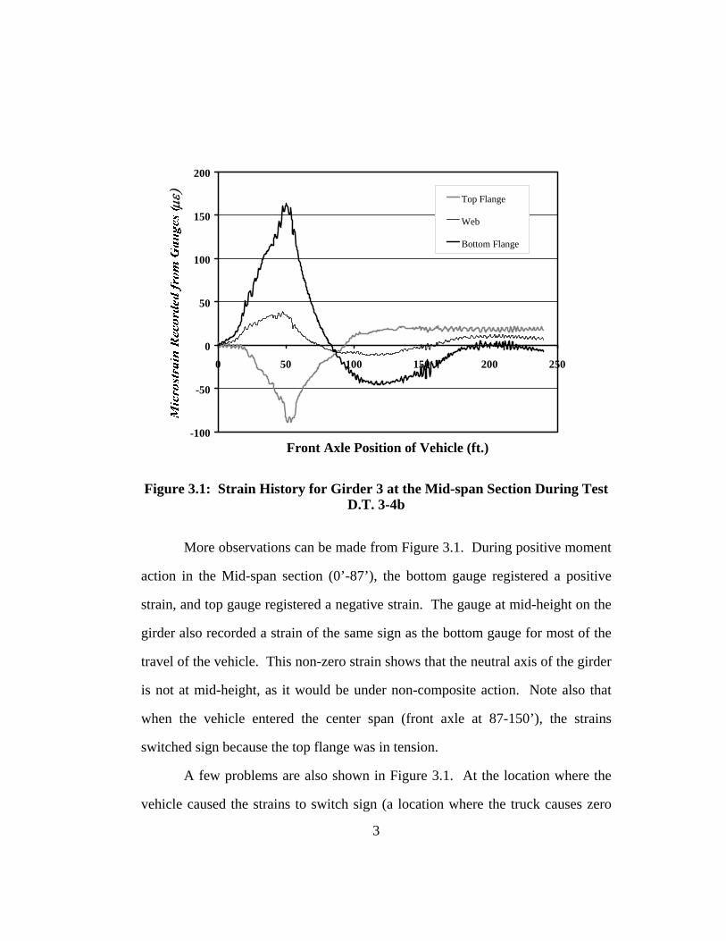
Plots were made of the raw data in microstrain. Figure 3.1 is a typical

example of a plot from any of the low-speed test runs. The figure shows strains

measured on one girder at the Mid-span section (35’ from beginning of bridge).

Extreme strains were recorded when the front axle of the dump truck was at

approximately 55’. This makes sense because the rear axles are 13.4’ and 17.9’

from the front axle and carry the greatest load. When the front axle is at

approximately 55’, the tandem was directly over the Mid-span section.

2

-100

-50

0

50

100

150

200

0 50 100 150 200 250

Front Axle Position of Vehicle (ft.)

με)

Top Flange

Web

Bottom Flange

Figure 3.1: Strain History for Girder 3 at the Mid-span Section During Test D.T. 3-4b

More observations can be made from Figure 3.1. During positive moment

action in the Mid-span section (0’-87’), the bottom gauge registered a positive

strain, and top gauge registered a negative strain. The gauge at mid-height on the

girder also recorded a strain of the same sign as the bottom gauge for most of the

travel of the vehicle. This non-zero strain shows that the neutral axis of the girder

is not at mid-height, as it would be under non-composite action. Note also that

when the vehicle entered the center span (front axle at 87-150’), the strains

switched sign because the top flange was in tension.

A few problems are also shown in Figure 3.1. At the location where the

vehicle caused the strains to switch sign (a location where the truck causes zero

3

moment at the section), a negative strain was recorded in all three gauges. This

indicated some degree of interaction with the deck slab. After the vehicle moves

far from the section (front axle position 150-250’) the web and top flange gages

registered a positive strain value, also indicating some interaction with the deck.

Oscillations could be seen in Figure 3.1 as well as most of the strain data, but

were limited to ±5με in most low-speed test runs.

3.2. CHANNEL SUMMARY

The system of gauges, completion boxes, junction boxes, and the CR9000

was complex enough that errors and malfunctioning channels could not always be

remedied in the field. A total of thirty-six steel gauges were used in the Leon

River test. Three gauges did not register strain readings for any of the tests. Two

of the gauges were located on the bottom flange of girder 2, one at the Mid-span

location and one at the Support location. The other non-working gauge was

located at mid-height on girder 1 at the Mid-span section. The missing gauge data

was estimated in a spreadsheet using similar triangles. This was done based on

the assumption that plain sections remain plane. The calculation was done with

confidence because two of the three gauges at each section still registered

reasonable strain values.

3.3. NOTABLE TEST RUNS

If a problem with a vehicle test was noticed in the field, the vehicle was

repositioned for a replicate run. There was one case where a problem was noticed

upon review of the preliminary data. In addition, the high-speed runs had larger

and quicker oscillations that needed special treatment. This section explains what

4

was done to these test runs in order to make them usable for the rest of this

research.

3.3.1. Fast Vehicle Tests

There were two sets of data that were acquired from high-speed vehicle

tests. One run was done with each vehicle. The speed of the dump truck was

approximately 55mph. The speed of the HETS vehicle was approximately

40mph. The impact of the vehicle with the bridge, the vibration of the vehicle, or

some combination of both effects could have caused the vibration in the bridge

system. The frequency of the oscillations caused by the dump truck was

approximately 0.5hz. The HETS vehicle caused oscillations that were hard to

distinguish from the typical noise of the data acquisition process.

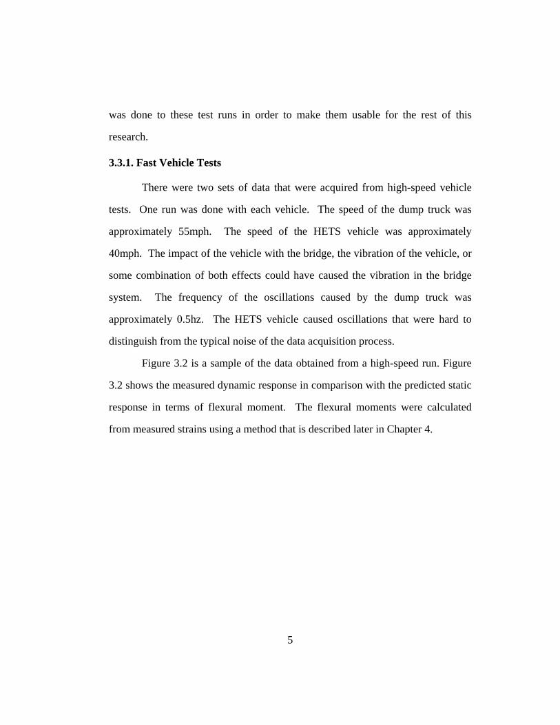
Figure 3.2 is a sample of the data obtained from a high-speed run. Figure

3.2 shows the measured dynamic response in comparison with the predicted static

response in terms of flexural moment. The flexural moments were calculated

from measured strains using a method that is described later in Chapter 4.

5

-500

-400

-300

-200

-100

0

100

200

0 50 100 150 200 250

Front Axle Position (ft.)

Predicted Static Response

Test D.T. H.S.

Figure 3.2: An Example of Vibration in a High-speed Test

Note that the mean of the dynamic response follows the static response quite well.

In order for the data from the high-speed tests to be usable for this research, the

oscillations needed to be filtered out.

Figure 3.3 shows another example from high-speed dump truck run, this

time showing the River section. Filtered data is also shown in Figure 3.3.

6

-400

-300

-200

-100

0

100

200

300

400

500

600

700

800

900

0 50 100 150 200 250

Front Axle Position (ft.)

Predicted Static Response

Test D.T.H.S. (Unfiltered)

Test D.T.H.S. (21 pt. filter)

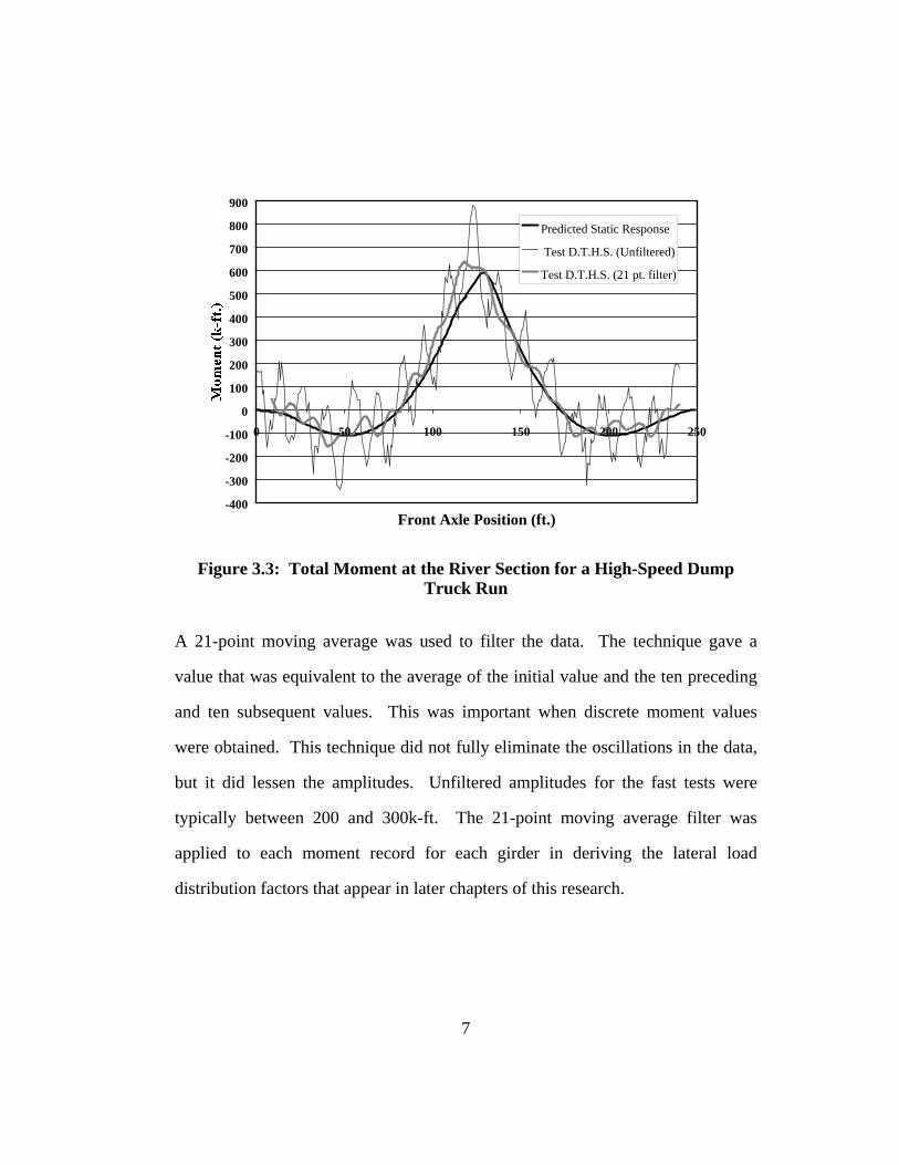
Figure 3.3: Total Moment at the River Section for a High-Speed Dump Truck Run

A 21-point moving average was used to filter the data. The technique gave a

value that was equivalent to the average of the initial value and the ten preceding

and ten subsequent values. This was important when discrete moment values

were obtained. This technique did not fully eliminate the oscillations in the data,

but it did lessen the amplitudes. Unfiltered amplitudes for the fast tests were

typically between 200 and 300k-ft. The 21-point moving average filter was

applied to each moment record for each girder in deriving the lateral load

distribution factors that appear in later chapters of this research.

7

3.4. CORRECTION OF FIRST DUMP TRUCK TEST

During vehicle test runs, a manual switch was used to mark the data

records to indicate the vehicle position. An observer was placed in position to see

the vehicle wheels cross the designated lane marks. The spacing of these marks

was given in Figure 1.18. The observer opened the switch as the front wheel of

the test vehicle passed a mark. The switch momentarily opened the excitation

channel and produced a zero voltage. This effect was seen in the acquired data

and was used data reduction. When test data was plotted against the line girder

data for the same vehicle, the voltage marks were the method of plotting the

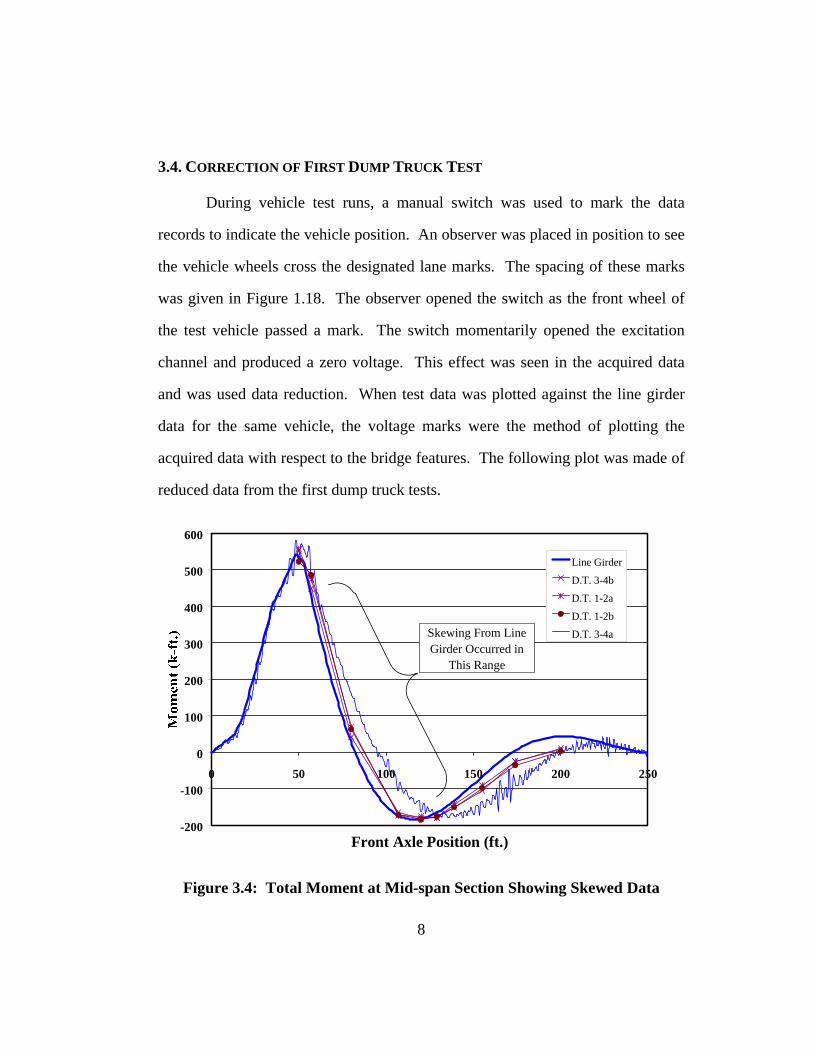
acquired data with respect to the bridge features. The following plot was made of

reduced data from the first dump truck tests.

-200

-100

0

100

200

300

400

500

600

0 50 100 150 200 250

Front Axle Position (ft.)

Line Girder

D.T. 3-4b

D.T. 1-2a

D.T. 1-2b

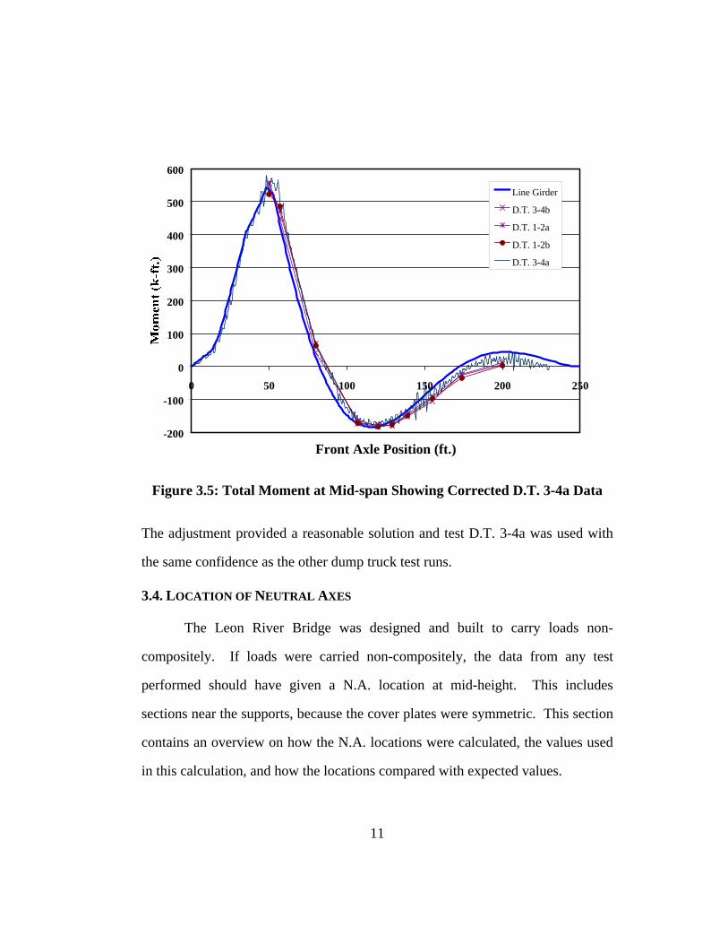
D.T. 3-4aSkewing From Line Girder Occurred in

This Range

Figure 3.4: Total Moment at Mid-span Section Showing Skewed Data

8

The data from test D.T.3-4a appears to skew from the other dump truck test and

line girder moment. This is the only test that exhibited this behavior. Sample

points taken from the other three dump truck tests fit the line girder analysis line

well. Also note that a definite point at which the data starts skewing from the

line-girder values is not visible. A solution was found in the voltage marks.

During a test, the vehicle tried to maintain constant speed. Therefore the

number of data records between each voltage mark should have been somewhat

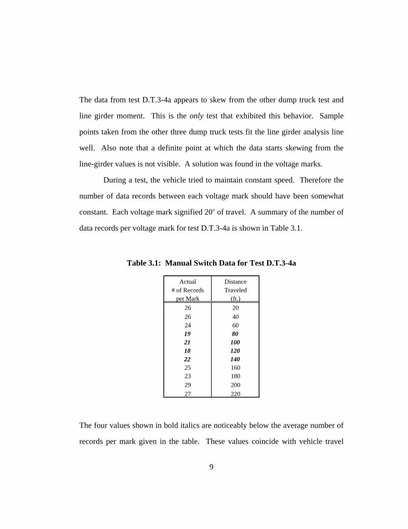
constant. Each voltage mark signified 20’ of travel. A summary of the number of

data records per voltage mark for test D.T.3-4a is shown in Table 3.1.

Table 3.1: Manual Switch Data for Test D.T.3-4a

Actual Distance# of Records Traveled

per Mark (ft.)26 2026 4024 6019 8021 10018 12022 14025 16023 18029 20027 220

The four values shown in bold italics are noticeably below the average number of

records per mark given in the table. These values coincide with vehicle travel

9

from 80’ to 140’, which is where the data for the test skews in Figure 3.4.

Although the switch operator did not make any notes at the time of the test, it

appeared as though and extra mark was added in this interval. The effect of this

would be to gradually put the truck out of position over a span of 60’ of travel.

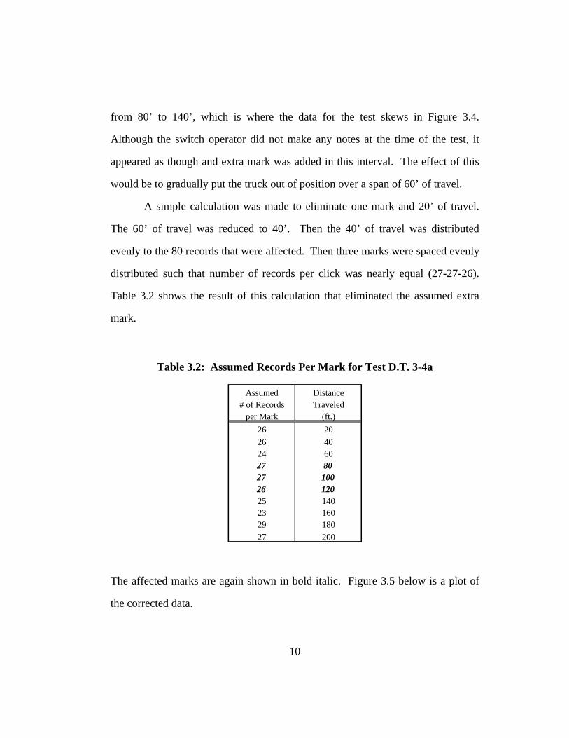
A simple calculation was made to eliminate one mark and 20’ of travel.

The 60’ of travel was reduced to 40’. Then the 40’ of travel was distributed

evenly to the 80 records that were affected. Then three marks were spaced evenly

distributed such that number of records per click was nearly equal (27-27-26).

Table 3.2 shows the result of this calculation that eliminated the assumed extra

mark.

Table 3.2: Assumed Records Per Mark for Test D.T. 3-4a

Assumed Distance# of Records Traveled

per Mark (ft.)26 2026 4024 6027 8027 10026 12025 14023 16029 18027 200

The affected marks are again shown in bold italic. Figure 3.5 below is a plot of

the corrected data.

10

-200

-100

0

100

200

300

400

500

600

0 50 100 150 200 250

Front Axle Position (ft.)

Line Girder

D.T. 3-4b

D.T. 1-2a

D.T. 1-2b

D.T. 3-4a

Figure 3.5: Total Moment at Mid-span Showing Corrected D.T. 3-4a Data

The adjustment provided a reasonable solution and test D.T. 3-4a was used with

the same confidence as the other dump truck test runs.

3.4. LOCATION OF NEUTRAL AXES

The Leon River Bridge was designed and built to carry loads non-

compositely. If loads were carried non-compositely, the data from any test

performed should have given a N.A. location at mid-height. This includes

sections near the supports, because the cover plates were symmetric. This section

contains an overview on how the N.A. locations were calculated, the values used

in this calculation, and how the locations compared with expected values.

11

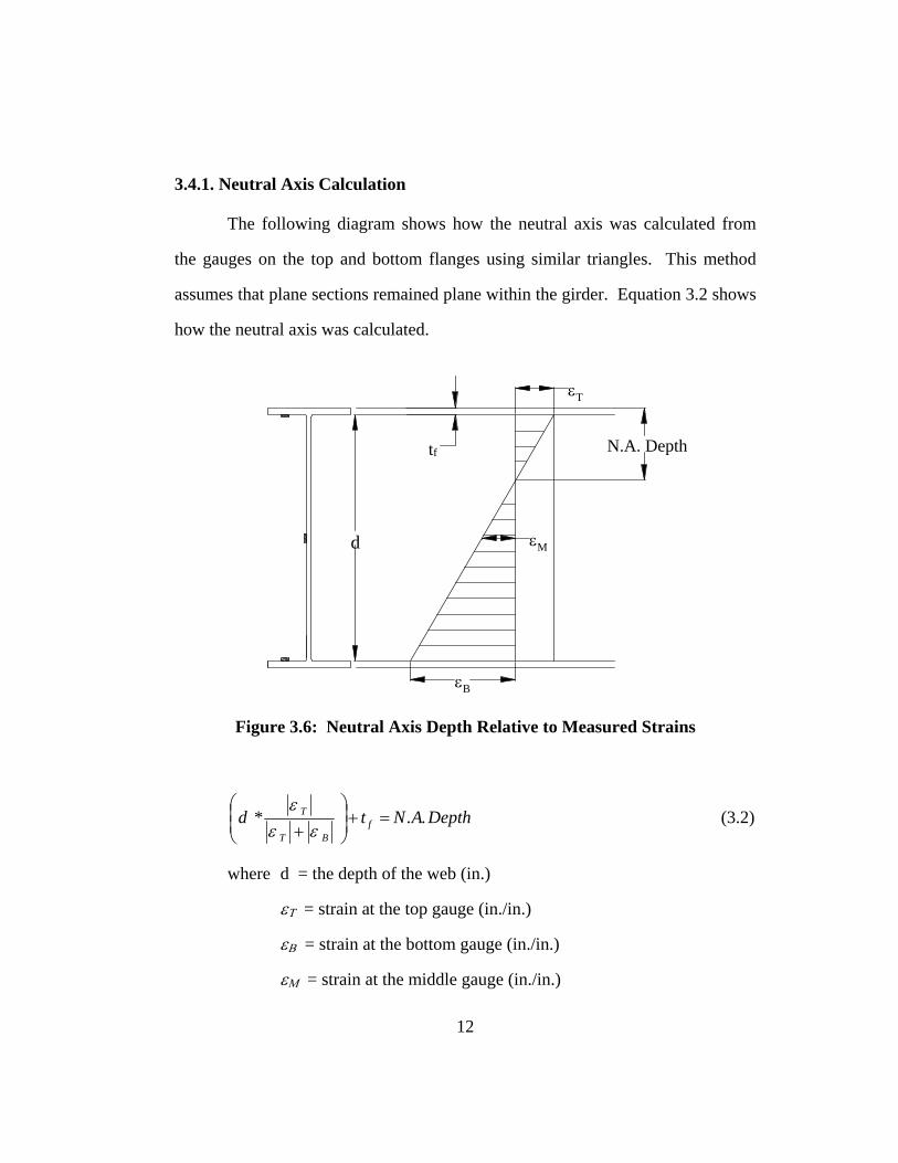
3.4.1. Neutral Axis Calculation

The following diagram shows how the neutral axis was calculated from

the gauges on the top and bottom flanges using similar triangles. This method

assumes that plane sections remained plane within the girder. Equation 3.2 shows

how the neutral axis was calculated.

d

N.A. Depth

εT

εB

tf

εM

Figure 3.6: Neutral Axis Depth Relative to Measured Strains

DepthANtd fBT

T ..* =+⎟⎟⎠

⎞⎜⎜⎝

⎛

+ εεε

(3.2)

where d = the depth of the web (in.)

εΤ = strain at the top gauge (in./in.)

εΒ = strain at the bottom gauge (in./in.)

εΜ = strain at the middle gauge (in./in.)

12

tf = flange thickness (in.)

There was another indication of neutral axis position. Gauges were placed

at the center of all girder sections. If the neutral axis were at mid-height of the

girders, there would have been zero strain at gauges placed at the center. Even if

the electrical noise was considered, substantial strains were present in all of the

gauges at mid-height.

3.4.2. Values Used in Neutral Axis Calculation

The N.A. positions calculated using Equation 3.2 for the full length of

travel of the test vehicle were not conclusive. Vibration, electrical oscillation, and

changes in moment action seemed to contribute to this. A plot of the calculated

N.A. position for the three girders with working gauges at the Mid-span section is

given in Figure 3.7.

13

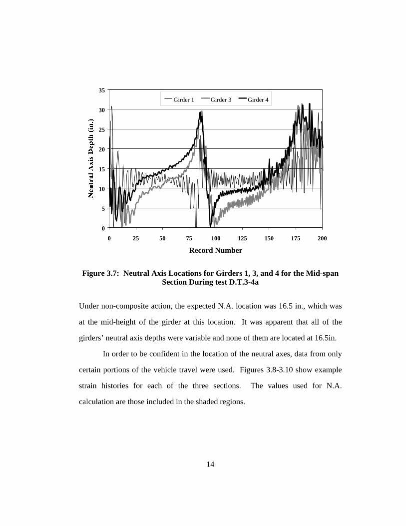
0

5

10

15

20

25

30

35

0 25 50 75 100 125 150 175 200

Record Number

Girder 1 Girder 3 Girder 4

Figure 3.7: Neutral Axis Locations for Girders 1, 3, and 4 for the Mid-span Section During test D.T.3-4a

Under non-composite action, the expected N.A. location was 16.5 in., which was

at the mid-height of the girder at this location. It was apparent that all of the

girders’ neutral axis depths were variable and none of them are located at 16.5in.

In order to be confident in the location of the neutral axes, data from only

certain portions of the vehicle travel were used. Figures 3.8-3.10 show example

strain histories for each of the three sections. The values used for N.A.

calculation are those included in the shaded regions.

14

-50

-25

0

25

50

75

100

0 50 100 150 200 250

Front Axle Position of Vehicle (ft.)

με Top FlangeWebBottom Flange

Figure 3.8: Girder 3 Strains at the Mid-span Section Showing Range of Values used for Neutral Axis Calculations

-100

-50

0

50

100

150

0 50 100 150 200 250

Front Axle Position of Vehicle (ft.)

με Top FlangeWebBottom Flange

Figure 3.9: Girder 1 Strains at the Support Section Showing Range of Values used for Neutral Axis Calculations

15

-200

-150

-100

-50

0

50

100

150

200

0 50 100 150 200 250

Front Axle Position of Vehicle (ft.)

με Top FlangeWebBottom Flange

Figure 3.10: Girder 1 Strains at the River Section Showing Range of Values used for Neutral Axis Calculations

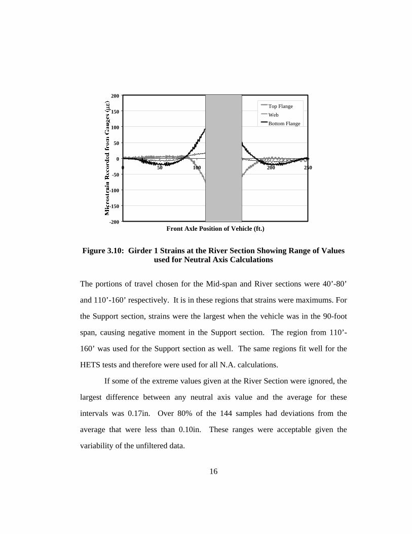
The portions of travel chosen for the Mid-span and River sections were 40’-80’

and 110’-160’ respectively. It is in these regions that strains were maximums. For

the Support section, strains were the largest when the vehicle was in the 90-foot

span, causing negative moment in the Support section. The region from 110’-

160’ was used for the Support section as well. The same regions fit well for the

HETS tests and therefore were used for all N.A. calculations.

If some of the extreme values given at the River Section were ignored, the

largest difference between any neutral axis value and the average for these

intervals was 0.17in. Over 80% of the 144 samples had deviations from the

average that were less than 0.10in. These ranges were acceptable given the

variability of the unfiltered data.

16

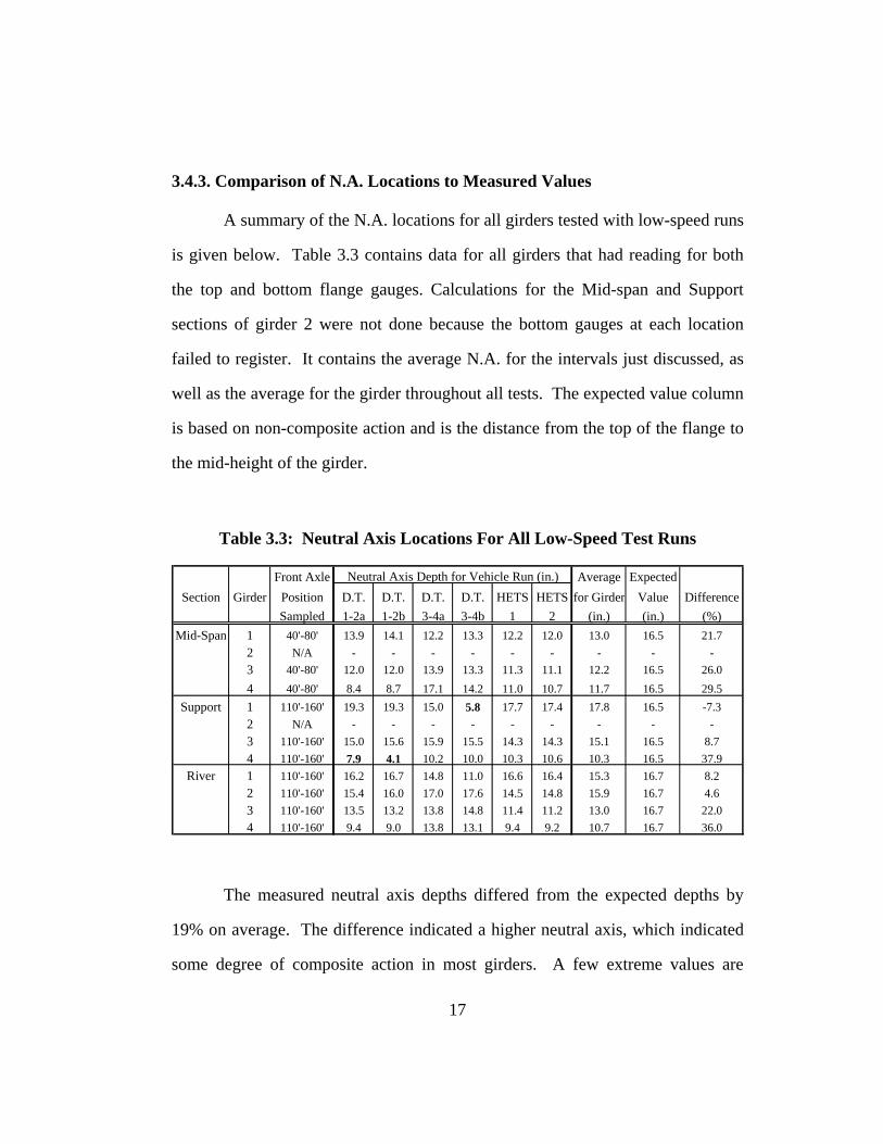
3.4.3. Comparison of N.A. Locations to Measured Values

A summary of the N.A. locations for all girders tested with low-speed runs

is given below. Table 3.3 contains data for all girders that had reading for both

the top and bottom flange gauges. Calculations for the Mid-span and Support

sections of girder 2 were not done because the bottom gauges at each location

failed to register. It contains the average N.A. for the intervals just discussed, as

well as the average for the girder throughout all tests. The expected value column

is based on non-composite action and is the distance from the top of the flange to

the mid-height of the girder.

Table 3.3: Neutral Axis Locations For All Low-Speed Test Runs

Front Axle Average ExpectedSection Girder Position D.T. D.T. D.T. D.T. HETS HETS for Girder Value Difference

Sampled 1-2a 1-2b 3-4a 3-4b 1 2 (in.) (in.) (%)Mid-Span 1 40'-80' 13.9 14.1 12.2 13.3 12.2 12.0 13.0 16.5 21.7

2 N/A - - - - - - - - -3 40'-80' 12.0 12.0 13.9 13.3 11.3 11.1 12.2 16.5 26.04 40'-80' 8.4 8.7 17.1 14.2 11.0 10.7 11.7 16.5 29.5

Support 1 110'-160' 19.3 19.3 15.0 5.8 17.7 17.4 17.8 16.5 -7.32 N/A - - - - - - - - -3 110'-160' 15.0 15.6 15.9 15.5 14.3 14.3 15.1 16.5 8.74 110'-160' 7.9 4.1 10.2 10.0 10.3 10.6 10.3 16.5 37.9

River 1 110'-160' 16.2 16.7 14.8 11.0 16.6 16.4 15.3 16.7 8.22 110'-160' 15.4 16.0 17.0 17.6 14.5 14.8 15.9 16.7 4.63 110'-160' 13.5 13.2 13.8 14.8 11.4 11.2 13.0 16.7 22.04 110'-160' 9.4 9.0 13.8 13.1 9.4 9.2 10.7 16.7 36.0

Neutral Axis Depth for Vehicle Run (in.)

The measured neutral axis depths differed from the expected depths by

19% on average. The difference indicated a higher neutral axis, which indicated

some degree of composite action in most girders. A few extreme values are

17

18

shown in bold. The most profound differences in every girder at a section were in

the Mid-span data for both the dump truck and heavy vehicle.

Chapter 4: Moment Calculation Techniques

The chapter will describe the calculation of moment from the strain data.

The method of calculation depends on the assumed bridge behavior. The Leon

River Bridge was designed non-compositely, but may not have behaved that way.

The strain data needed a method of data reduction that was appropriate to the

bridge behavior. In addition, the participation of the curbs in the flexural

response of the bridge was in question. Therefore, a few different moment

calculation techniques were used. The criterion for judging data reduction

techniques was how well a summation of moments across a section matched the

static line girder value.

4.1. Sampling Intervals

The summation of moments was done at the seven selected vehicle

positions given in Table 2.2. The values of moment were based on an average to

filter the noise in the data. The average moment value was calculated by

averaging the three to four values that were contained within the range of data

acquired one foot before and one foot after the vehicle location in question. In

effect, for locations of maximum moment, the average moment underestimated

the peak moment. The majority of the underestimates were within 5%, although

some were as large as 15%. This effect was considered negligible since it

eliminated some effects of oscillation and gave values acceptable for use in

moment distribution factors.

1

4.2. MOMENT CALCULATION TECHNIQUES

There were two aspects of bridge behavior that needed to be dealt with

when reducing the moments from the strain data. The first was the degree of

composite action of the deck with the girders. The second was the contribution of

the curbs if some composite action was assumed. The preliminary N.A. location

information gave an indication that the girders and deck were acting compositely

to some degree. The various ways to model the curbs is given first in this section

before data reduction techniques are given.

4.2.1. Properties of the Contributing Curb Sections

The basis for the calculations in this section comes from the equation for

moment given in Equation 4.1.

⎟⎠⎞

⎜⎝⎛=

cIEM ε (4.1)

where M = flexural moment in the girder (k-ft)

ε = strain at a given location on the girder (in./in.)

E = elastic modulus for steel = 29,000ksi

I = moment of inertia of the section (in4)

c = distance from the neutral axis to the location of strain, ε (in.)

The critical value in the calculation of flexural response from the recorded strains

was the value of I/c for the exterior girder sections. The value of I/c is called the

section modulus, and will be referred to as SCG to signify the use of the value of c

that is the distance from the neutral axis to the location of the gage, not the

2

extreme fiber. Four possibilities for SCG were considered in this research. One

was based on non-composite action and three were based on composite action.

4.2.1.1. Calculation of SCG for Non-composite Sections

Where non-composite behavior was assumed, the value of SCG used for

each W-shape was the standard value of I for the W-shape, divided by the

distance from mid-height of the W-shape to the location of the bottom flange

gage, c. Gages were attached on the top of the bottom flange as shown previously

in Figures 1.6 and 1.7. Therefore, considering non-composite action, the values

of c for the W33x130 and W33x141 alone were simply half the total height of the

shape minus the thickness of one flange. The value of c was 15.69” for both W

shapes. The value of I is 6710in4 for the W33x130 and 7450in4 for the W33x141.

The value of SCG was equal to 428in3 for the W33x130 and equal to 475in3 for the

W33x141.

4.2.1.2. Calculation of SCG for Composite Sections

For the interior girders, the effective width for composite action was taken

as half the distance between the flanges on both sides, plus the width over the

flange itself. However, the contributing concrete for an exterior girder was

different. Figure 4.1 shows a section view of the deck material over an exterior

girder.

3

9.0"

9.0"

34.0" 40.0"

80”

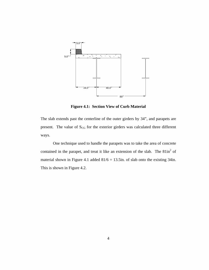
Figure 4.1: Section View of Curb Material

The slab extends past the centerline of the outer girders by 34”, and parapets are

present. The value of SCG for the exterior girders was calculated three different

ways.

One technique used to handle the parapets was to take the area of concrete

contained in the parapet, and treat it like an extension of the slab. The 81in2 of

material shown in Figure 4.1 added 81/6 = 13.5in. of slab onto the existing 34in.

This is shown in Figure 4.2.

4

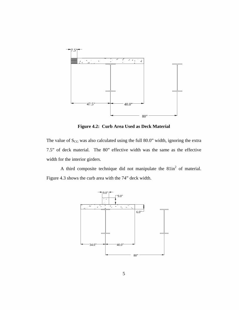
80”

40.0"47.5"

7.5"

Figure 4.2: Curb Area Used as Deck Material

The value of SCG was also calculated using the full 80.0” width, ignoring the extra

7.5” of deck material. The 80” effective width was the same as the effective

width for the interior girders.

A third composite technique did not manipulate the 81in2 of material.

Figure 4.3 shows the curb area with the 74” deck width.

80”

34.0" 40.0"

9.0" 9.0"

6.0"

5

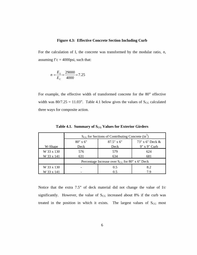
Figure 4.3: Effective Concrete Section Including Curb

For the calculation of I, the concrete was transformed by the modular ratio, n,

assuming f’c = 4000psi, such that:

25.7400029000

===C

S

EE

n

For example, the effective width of transformed concrete for the 80” effective

width was 80/7.25 = 11.03”. Table 4.1 below gives the values of SCG calculated

three ways for composite action.

Table 4.1. Summary of SCG Values for Exterior Girders

80" x 6" 87.5" x 6" 73" x 6" Deck &W-Shape Deck Deck 9" x 9" Curb

W 33 x 130 576 579 624W 33 x 141 631 634 681

W 33 x 130 - 0.5 8.2W 33 x 141 - 0.5 7.9

SCG for Sections of Contributing Concrete (in3)

Percentage Increase over SCG for 80" x 6" Deck

Notice that the extra 7.5” of deck material did not change the value of I/c

significantly. However, the value of SCG increased about 8% if the curb was

treated in the position in which it exists. The largest values of SCG most

6

accurately depict the cross-section and were used where appropriate in the

calculations that follow.

4.2.2. Non-composite Method of Moment Reduction

The first moment reduction technique assumed non-composite action.

Although the neutral axis locations indicated in Section 3.4.3 indicated a degree

of composite action, the data was first reduced assuming no composite action,

since that is how the bridge system was designed. The moment was related to

strain by Equation 4.2.

( ) 12*

CGSB S

EM

ε= (4.2)

where M = total moment in the girder (k-ft)

εB = strain in the bottom gauge (in/in)

Es = elastic modulus for steel = 29,000 ksi

SCG = modulus for the W-shape alone (in3) for strains at the

top of the bottom flange

4.2.3. Fully Composite Method

A better technique used for data reduction is one that recognizes the

neutral axis locations described in Section 3.4.3. Overall, the N.A. locations were

higher than mid-height. However, a wide range of N.A. depths are given in Table

3.3. The calculations of composite section modulus in Table 4.1 indicated a N.A.

depth of approximately 4.7in when considering the 80” or 87.5” x 6” contributing

slab. The N.A. depth was approximately 0.02in (practically at the interface of the

7

steel and slab) for the 73” x 6” slab section and 9” portion of curb. These N.A.

locations are higher than those indicated in Table 3.3.

Instead of trying a method of partial composite action to reduce date from

girders that have varying N.A. depths, it was first assumed that all the girders

behaved in a fully composite manner. The value of SCG is the only variable that

changes in this method from the non-composite technique. The composite SCG

was calculated for both interior and exterior girders of both sizes. These were

given in Table 4.1. Moment reduction was performed using Equation 4.2 and was

the same as the CGM technique used by BRUFEM.

4.2.4. Moment-Couple Method

Another method of reducing the data in a fully composite manner was the

Moment-Couple technique outlined in detail in Jauregui (1999). This method is

similar to the EGM BRUFEM method discussed previously in Section 2.3.1.2. In

this method, four assumptions were made: 1. Plane sections remained plane over the depth of the girder and tributary slab

section, but not over the entire depth of the composite section. A strain discontinuity at the interface of the two materials was allowed.

2. The curvatures of the girder and tributary slab section were equivalent. 3. The tributary slab section stayed in contact with the girder but could move

longitudinally relative to the girder flanges. 4. There was no net axial force at the girder cross-section.

Under those assumptions, the total moment in the girder was equal to the

sum of three moments: the moment resisted by the girder alone, Mg, the moment

resisted by the effective slab width alone, Ms, and a moment from the equal and

8

opposite axial forces acting on the girder and slab, Mc. The forces involved in Mc

were caused by friction at the interface of the slab and girder. The moment comes

from the equal and opposite forces acting at an eccentricity, e, which was equal to

the distance between the neutral axes of the girder and slab. A diagram of the

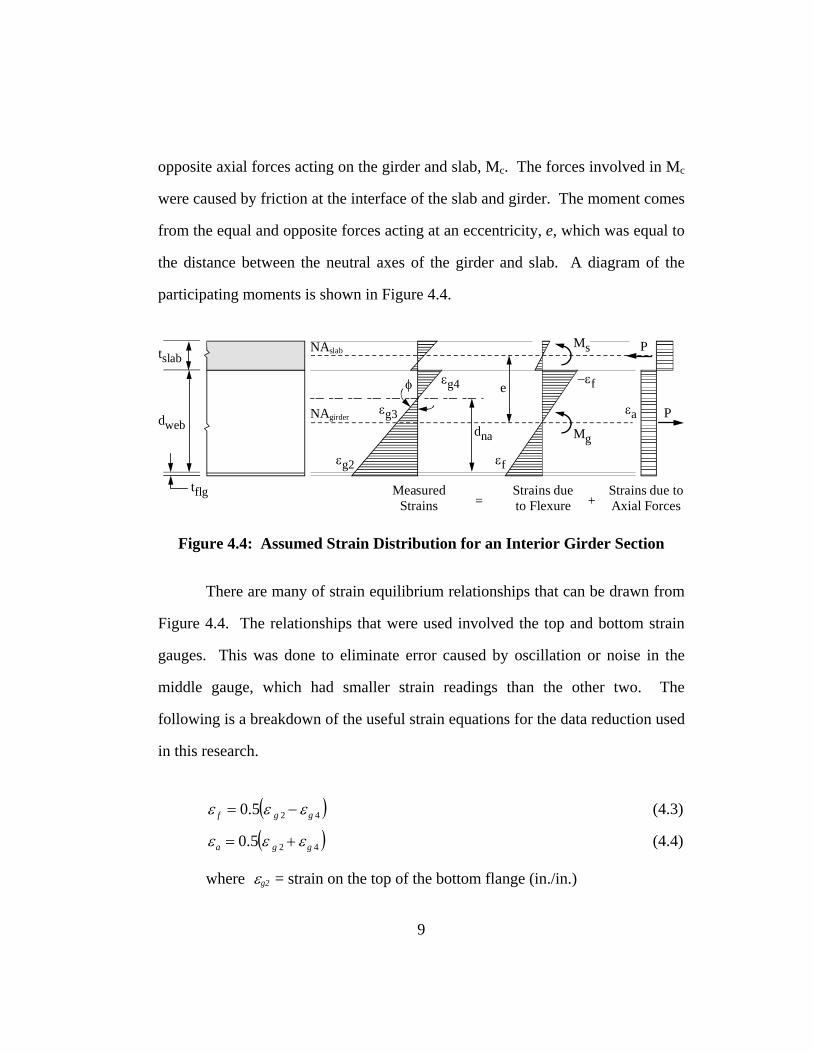
participating moments is shown in Figure 4.4.

εg2

εg3

εg4

εf

−εf

εadweb

tflg

tslab

Mg

Ms P

P

e

dna

NAgirder

NAslab

MeasuredStrains

Strains dueto Flexure

Strains due toAxial Forces= +

φ

Figure 4.4: Assumed Strain Distribution for an Interior Girder Section

There are many of strain equilibrium relationships that can be drawn from

Figure 4.4. The relationships that were used involved the top and bottom strain

gauges. This was done to eliminate error caused by oscillation or noise in the

middle gauge, which had smaller strain readings than the other two. The

following is a breakdown of the useful strain equations for the data reduction used

in this research.

( )425.0 ggf εεε −= (4.3)

( ) (4.4) 425.0 ggaε ε += ε

where εg2 = strain on the top of the bottom flange (in./in.)

9

εg4 = strain on the bottom of the top flange (in./in.)

εf = strain in pure flexure portion of girder action (in./in.)

εa = strain due to axial forces in girder (in./in.)

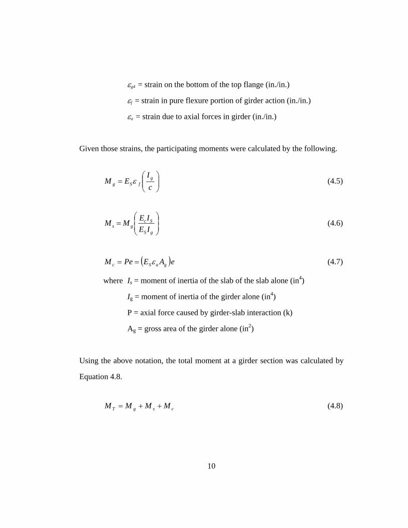
Given those strains, the participating moments were calculated by the following.

⎟⎟⎠

⎞⎜⎜⎝

⎛=

cI

EM gfSg ε (4.5)

⎟⎟⎠

⎞⎜⎜⎝

⎛=

gS

Scgs IE

IEMM (4.6)

( )eAEPeM gaSc ε== (4.7)

where Is = moment of inertia of the slab of the slab alone (in4)

Ig = moment of inertia of the girder alone (in4)

P = axial force caused by girder-slab interaction (k)

Ag = gross area of the girder alone (in2)

Using the above notation, the total moment at a girder section was calculated by

Equation 4.8.

csgT MMMM ++= (4.8)

10

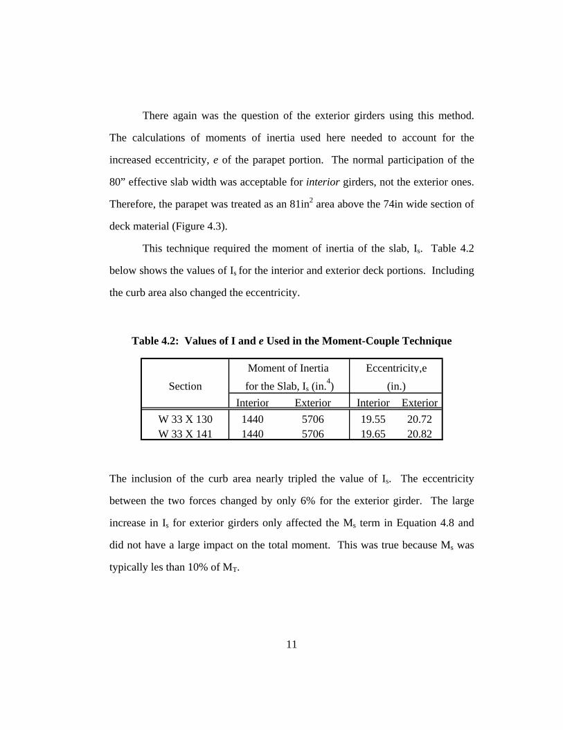
There again was the question of the exterior girders using this method.

The calculations of moments of inertia used here needed to account for the

increased eccentricity, e of the parapet portion. The normal participation of the

80” effective slab width was acceptable for interior girders, not the exterior ones.

Therefore, the parapet was treated as an 81in2 area above the 74in wide section of

deck material (Figure 4.3).

This technique required the moment of inertia of the slab, Is. Table 4.2

below shows the values of Is for the interior and exterior deck portions. Including

the curb area also changed the eccentricity.

Table 4.2: Values of I and e Used in the Moment-Couple Technique

SectionInterior Exterior Interior Exterior

W 33 X 130 1440 5706 19.55 20.72W 33 X 141 1440 5706 19.65 20.82

Moment of Inertia Eccentricity,efor the Slab, Is (in.4) (in.)

The inclusion of the curb area nearly tripled the value of Is. The eccentricity

between the two forces changed by only 6% for the exterior girder. The large

increase in Is for exterior girders only affected the Ms term in Equation 4.8 and

did not have a large impact on the total moment. This was true because Ms was

typically les than 10% of MT.

11

4.3. COMPARISON WITH SAP2000

The major criteria used when judging the data reduction methods was how

well moments summed across a section matched with the SAP2000 line girder

moment. This was done for all six slow vehicle runs, at the seven selected vehicle

locations. The three other zero moment locations were included as well because

they gave reasonable for total moment. Figures 4.7-4.24 show the results of

moment reduction using all three methods discussed in Sections 4.2.2-4.2.4.

Figure 4.5 is an example plot. It was taken from the data for the dump

truck over the River section. There a few key features that appear in the plot: 1. Each plotted point represents the total moment at the cross section for a single

test run. This total was calculated using Equation 4.9.

∑=4

1iTot MM (4.9)

where Μι = Moment on a girder calculated from strains measured from

the top of the bottom flange (k-in.)

ΜΤοτ = Total moment at a cross-section (k-in.)

2. The scatter of the values plotted at the same front axle location was small in

general. This indicated a good degree of repeatability in the acquired data. 3. The predicted static response, “Line Girder,” plotted near the test data or was

contained within the range of test data for a given vehicle location.

12

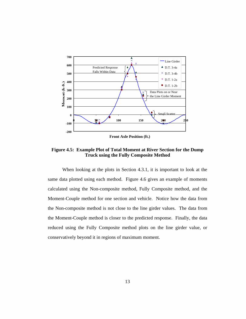
-200

-100

0

100

200

300

400

500

600

700

0 50 100 150 200 250

Front Axle Position (ft.)

Line Girder

D.T. 3-4a

D.T. 3-4b

D.T. 1-2a

D.T. 1-2b

Predicted Response Falls Within Data

Small Scatter

Data Plots on or Near the Line Girder Moment

Figure 4.5: Example Plot of Total Moment at River Section for the Dump Truck using the Fully Composite Method

When looking at the plots in Section 4.3.1, it is important to look at the

same data plotted using each method. Figure 4.6 gives an example of moments

calculated using the Non-composite method, Fully Composite method, and the

Moment-Couple method for one section and vehicle. Notice how the data from

the Non-composite method is not close to the line girder values. The data from

the Moment-Couple method is closer to the predicted response. Finally, the data

reduced using the Fully Composite method plots on the line girder value, or

conservatively beyond it in regions of maximum moment.

13

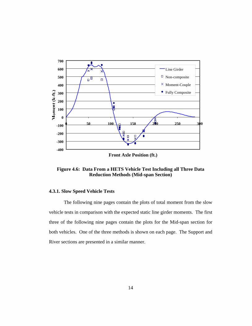
-400

-300

-200

-100

0

100

200

300

400

500

600

700

0 50 100 150 200 250 300

Front Axle Position (ft.)

Line Girder

Non-composite

Moment-Couple

Fully Composite

Figure 4.6: Data From a HETS Vehicle Test Including all Three Data Reduction Methods (Mid-span Section)

4.3.1. Slow Speed Vehicle Tests

The following nine pages contain the plots of total moment from the slow

vehicle tests in comparison with the expected static line girder moments. The first

three of the following nine pages contain the plots for the Mid-span section for

both vehicles. One of the three methods is shown on each page. The Support and

River sections are presented in a similar manner.

14

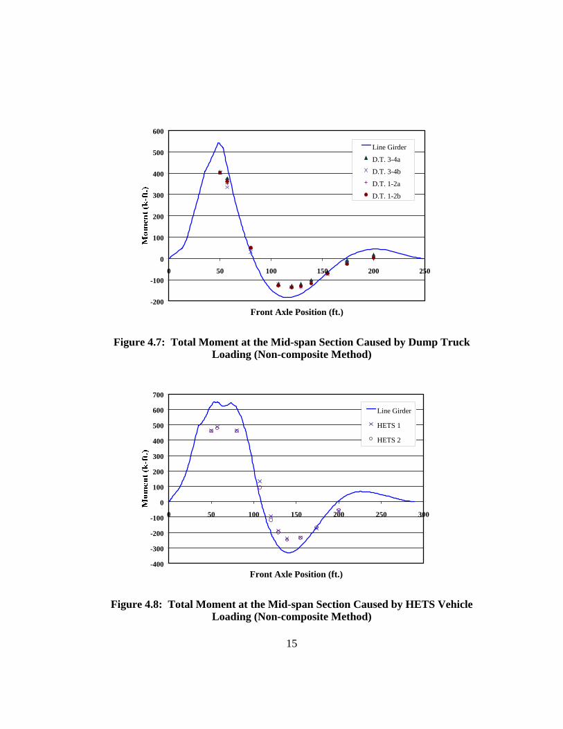
-200

-100

0

100

200

300

400

500

600

0 50 100 150 200 250

Front Axle Position (ft.)

Line Girder

D.T. 3-4a

D.T. 3-4b

D.T. 1-2a

D.T. 1-2b

Figure 4.7: Total Moment at the Mid-span Section Caused by Dump Truck Loading (Non-composite Method)

-400

-300

-200

-100

0

100

200

300

400

500

600

700

0 50 100 150 200 250 300

Front Axle Position (ft.)

Line Girder

HETS 1

HETS 2

Figure 4.8: Total Moment at the Mid-span Section Caused by HETS Vehicle Loading (Non-composite Method)

15

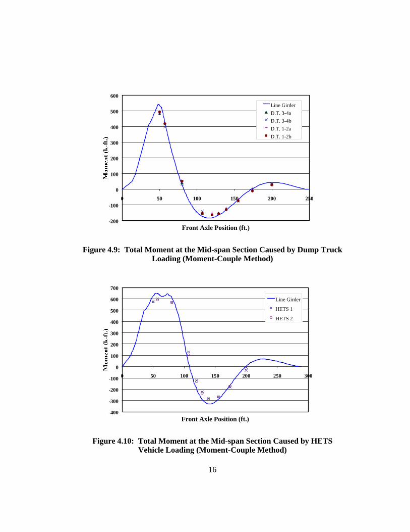
-200

-100

0

100

200

300

400

500

600

0 50 100 150 200 250

Front Axle Position (ft.)

Line GirderD.T. 3-4aD.T. 3-4bD.T. 1-2aD.T. 1-2b

Figure 4.9: Total Moment at the Mid-span Section Caused by Dump Truck Loading (Moment-Couple Method)

-400

-300

-200

-100

0

100

200

300

400

500

600

700

0 50 100 150 200 250 300

Front Axle Position (ft.)

Line Girder

HETS 1

HETS 2

Figure 4.10: Total Moment at the Mid-span Section Caused by HETS Vehicle Loading (Moment-Couple Method)

16

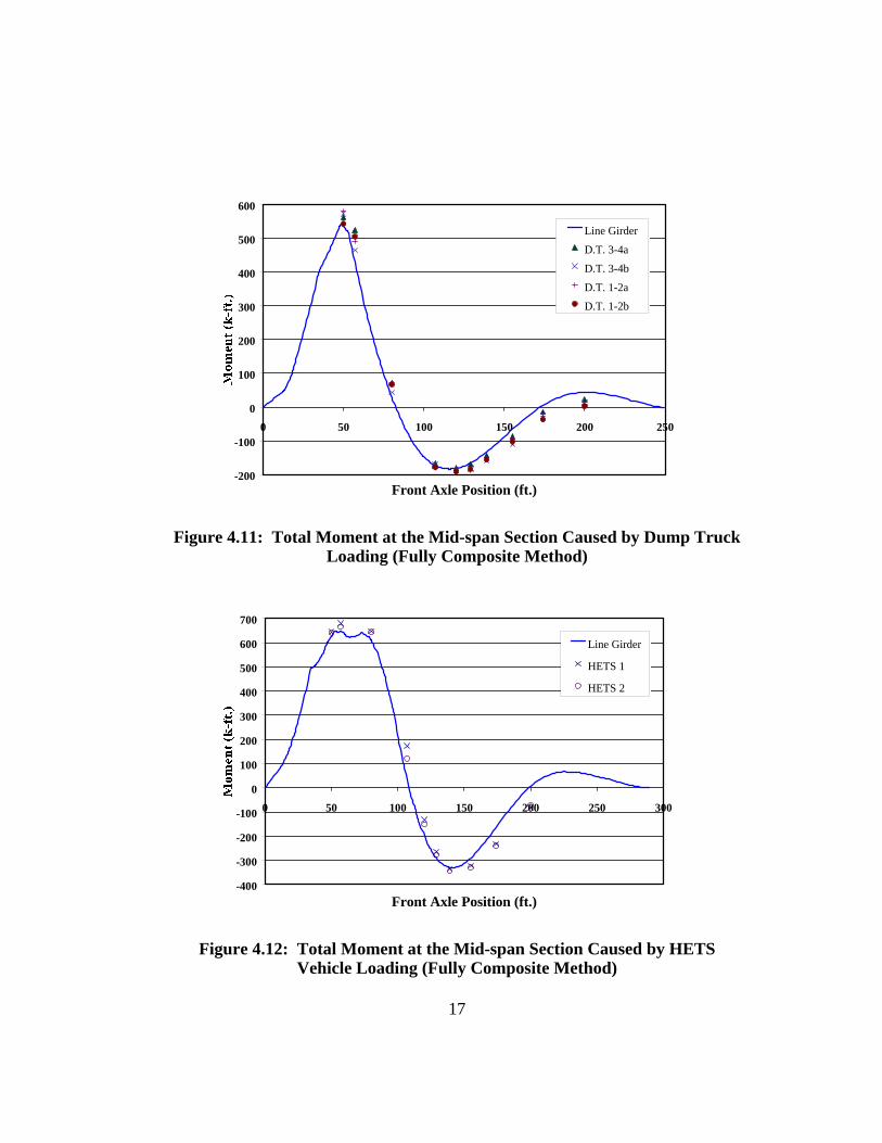
-200

-100

0

100

200

300

400

500

600

0 50 100 150 200 250

Front Axle Position (ft.)

Line Girder

D.T. 3-4a

D.T. 3-4b

D.T. 1-2a

D.T. 1-2b

Figure 4.11: Total Moment at the Mid-span Section Caused by Dump Truck Loading (Fully Composite Method)

-400

-300

-200

-100

0

100

200

300

400

500

600

700

0 50 100 150 200 250 300

Front Axle Position (ft.)

Line Girder

HETS 1

HETS 2

Figure 4.12: Total Moment at the Mid-span Section Caused by HETS Vehicle Loading (Fully Composite Method)

17

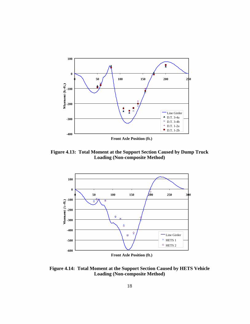
-400

-300

-200

-100

0

100

0 50 100 150 200 250

Front Axle Position (ft.)

Line GirderD.T. 3-4aD.T. 3-4bD.T. 1-2aD.T. 1-2b

Figure 4.13: Total Moment at the Support Section Caused by Dump Truck Loading (Non-composite Method)

-600

-500

-400

-300

-200

-100

0

100

0 50 100 150 200 250 300

Front Axle Position (ft.)

Line GirderHETS 1HETS 2

Figure 4.14: Total Moment at the Support Section Caused by HETS Vehicle Loading (Non-composite Method)

18

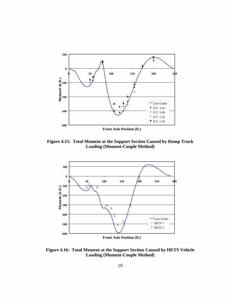
-400

-300

-200

-100

0

100

0 50 100 150 200 250

Front Axle Position (ft.)

Line GirderD.T. 3-4aD.T. 3-4bD.T. 1-2aD.T. 1-2b

Figure 4.15: Total Moment at the Support Section Caused by Dump Truck Loading (Moment-Couple Method)

-600

-500

-400

-300

-200

-100

0

100

0 50 100 150 200 250 300

Front Axle Position (ft.)

Line GirderHETS 1HETS 2

Figure 4.16: Total Moment at the Support Section Caused by HETS Vehicle Loading (Moment-Couple Method)

19

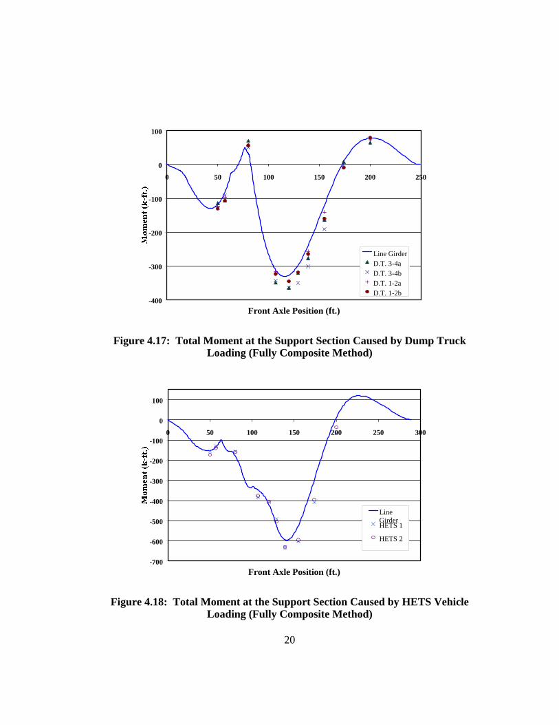
-400

-300

-200

-100

0

100

0 50 100 150 200 250

Front Axle Position (ft.)

Line GirderD.T. 3-4aD.T. 3-4bD.T. 1-2aD.T. 1-2b

Figure 4.17: Total Moment at the Support Section Caused by Dump Truck Loading (Fully Composite Method)

-700

-600

-500

-400

-300

-200

-100

0

100

0 50 100 150 200 250 300

Front Axle Position (ft.)

LineGirderHETS 1

HETS 2

Figure 4.18: Total Moment at the Support Section Caused by HETS Vehicle Loading (Fully Composite Method)

20

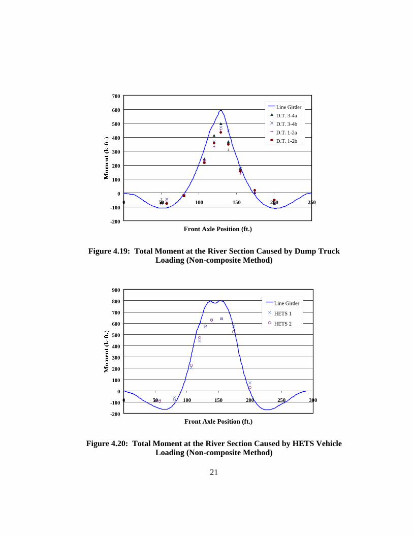
-200

-100

0

100

200

300

400

500

600

700

0 50 100 150 200 250

Front Axle Position (ft.)

Line GirderD.T. 3-4aD.T. 3-4bD.T. 1-2aD.T. 1-2b

Figure 4.19: Total Moment at the River Section Caused by Dump Truck Loading (Non-composite Method)

-200

-100

0

100

200

300

400

500

600

700

800

900

0 50 100 150 200 250 300

Front Axle Position (ft.)

Line Girder

HETS 1

HETS 2

Figure 4.20: Total Moment at the River Section Caused by HETS Vehicle Loading (Non-composite Method)

21

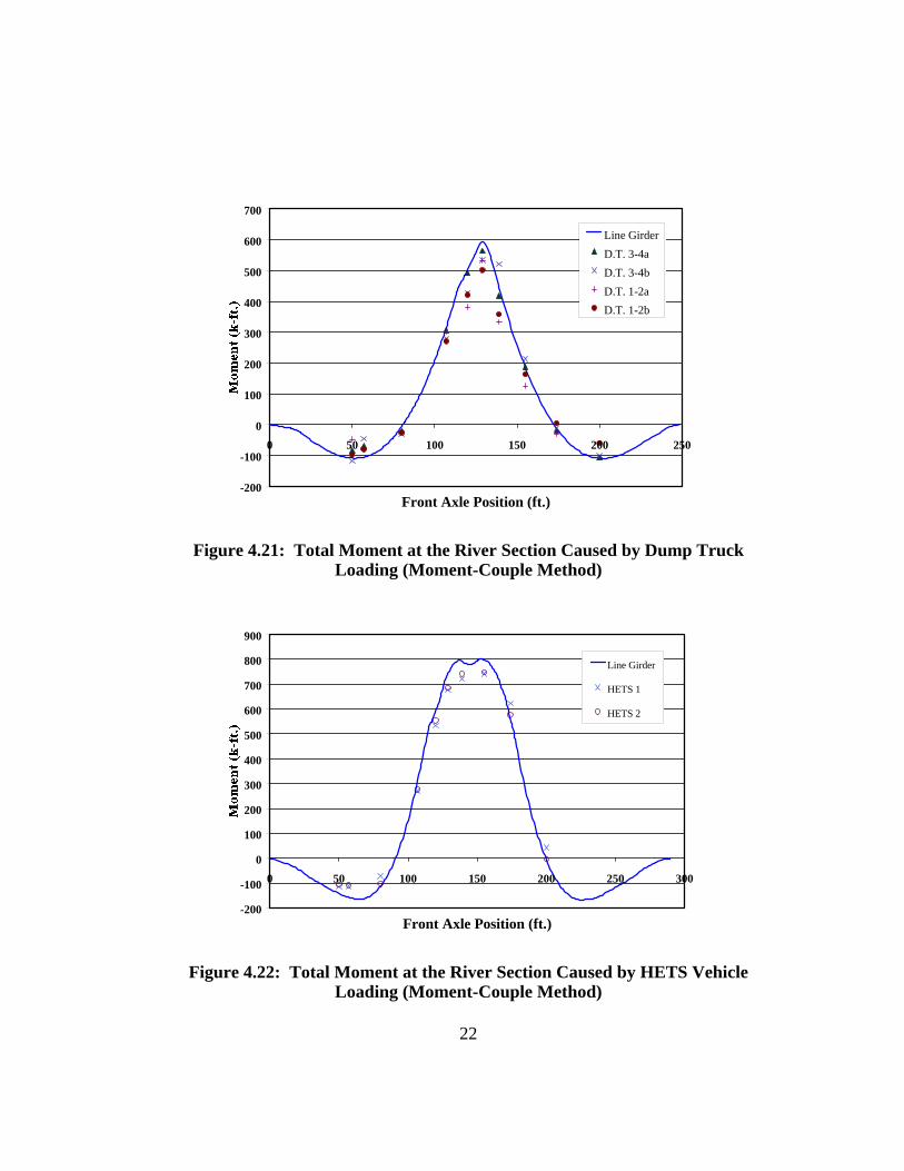
-200

-100

0

100

200

300

400

500

600

700

0 50 100 150 200 250

Front Axle Position (ft.)

Line GirderD.T. 3-4aD.T. 3-4bD.T. 1-2aD.T. 1-2b

Figure 4.21: Total Moment at the River Section Caused by Dump Truck Loading (Moment-Couple Method)

-200

-100

0

100

200

300

400

500

600

700

800

900

0 50 100 150 200 250 300

Front Axle Position (ft.)

Line Girder

HETS 1

HETS 2

Figure 4.22: Total Moment at the River Section Caused by HETS Vehicle Loading (Moment-Couple Method)

22

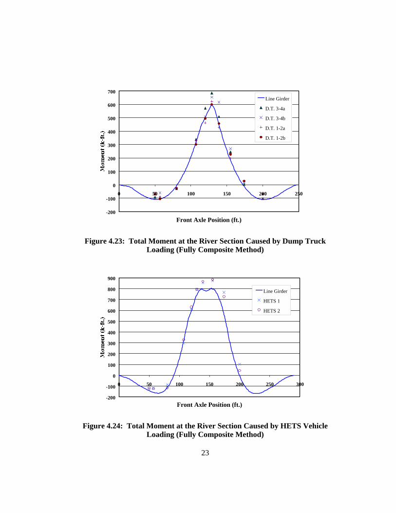
-200

-100

0

100

200

300

400

500

600

700

0 50 100 150 200 250

Front Axle Position (ft.)

Line Girder

D.T. 3-4a

D.T. 3-4b

D.T. 1-2a

D.T. 1-2b

Figure 4.23: Total Moment at the River Section Caused by Dump Truck Loading (Fully Composite Method)

-200

-100

0

100

200

300

400

500

600

700

800

900

0 50 100 150 200 250 300

Front Axle Position (ft.)

Line Girder

HETS 1

HETS 2

Figure 4.24: Total Moment at the River Section Caused by HETS Vehicle Loading (Fully Composite Method)

23

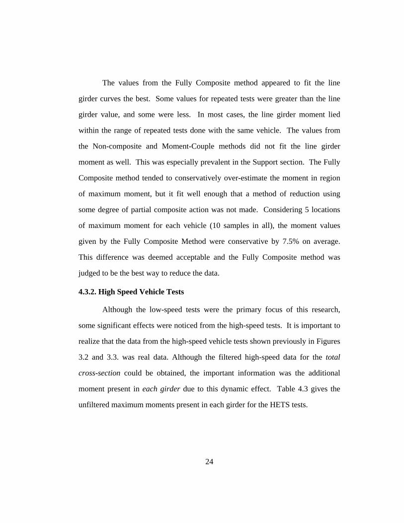
The values from the Fully Composite method appeared to fit the line

girder curves the best. Some values for repeated tests were greater than the line

girder value, and some were less. In most cases, the line girder moment lied

within the range of repeated tests done with the same vehicle. The values from

the Non-composite and Moment-Couple methods did not fit the line girder

moment as well. This was especially prevalent in the Support section. The Fully

Composite method tended to conservatively over-estimate the moment in region

of maximum moment, but it fit well enough that a method of reduction using

some degree of partial composite action was not made. Considering 5 locations

of maximum moment for each vehicle (10 samples in all), the moment values

given by the Fully Composite Method were conservative by 7.5% on average.

This difference was deemed acceptable and the Fully Composite method was

judged to be the best way to reduce the data.

4.3.2. High Speed Vehicle Tests

Although the low-speed tests were the primary focus of this research,

some significant effects were noticed from the high-speed tests. It is important to

realize that the data from the high-speed vehicle tests shown previously in Figures

3.2 and 3.3. was real data. Although the filtered high-speed data for the total

cross-section could be obtained, the important information was the additional

moment present in each girder due to this dynamic effect. Table 4.3 gives the

unfiltered maximum moments present in each girder for the HETS tests.

24

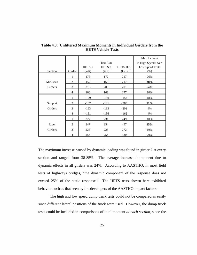
Table 4.3: Unfiltered Maximum Moments in Individual Girders from the HETS Vehicle Tests

Max Increasein High Speed Over

HETS 1 HETS 2 HETS H.S. Low Speed TestsSection Girder (k-ft) (k-ft) (k-ft) (%)

1 175 172 217 26%

Mid-span 2 157 160 217 38%Girders 3 213 208 201 -4%

4 166 161 177 10%

1 -129 -130 -152 18%

Support 2 -187 -191 -283 51%

Girders 3 -193 -193 -201 4%4 -161 -156 -162 4%

1 227 231 249 10%

River 2 247 254 457 85%

Girders 3 228 228 272 19%4 256 258 330 29%

Test Run

The maximum increase caused by dynamic loading was found in girder 2 at every

section and ranged from 38-85%. The average increase in moment due to

dynamic effects in all girders was 24%. According to AASTHO, in most field

tests of highways bridges, “the dynamic component of the response does not

exceed 25% of the static response.” The HETS tests shown here exhibited

behavior such as that seen by the developers of the AASTHO impact factors.

The high and low speed dump truck tests could not be compared as easily

since different lateral positions of the truck were used. However, the dump truck

tests could be included in comparisons of total moment at each section, since the

25

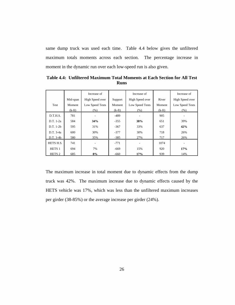
same dump truck was used each time. Table 4.4 below gives the unfiltered

maximum totals moments across each section. The percentage increase in

moment in the dynamic run over each low-speed run is also given.

Table 4.4: Unfiltered Maximum Total Moments at Each Section for All Test Runs

Increase of Increase of Increase of

Mid-span High Speed over Support High Speed over River High Speed over

Test Moment Low Speed Tests Moment Low Speed Tests Moment Low Speed Tests(k-ft) (%) (k-ft) (%) (k-ft) (%)

D.T.H.S. 781 - -489 - 905 -

D.T. 1-2a 584 34% -355 38% 651 39%

D.T. 1-2b 595 31% -367 33% 637 42%

D.T. 3-4a 600 30% -377 30% 718 26%D.T. 3-4b 580 35% -385 27% 717 26%

HETS H.S. 741 - -771 - 1074 -

HETS 1 694 7% -669 15% 920 17%HETS 2 685 8% -660 17% 939 14%

The maximum increase in total moment due to dynamic effects from the dump

truck was 42%. The maximum increase due to dynamic effects caused by the

HETS vehicle was 17%, which was less than the unfiltered maximum increases

per girder (38-85%) or the average increase per girder (24%).

26

Chapter 5: Distribution of Moment With Vehicle Position

Information in Chapter 3 indicated that the Leon River Bridge exhibited

some degree of composite action. The Fully Composite gave total moments that

fit the line girder values very well. It was this method that was applied to all the

data used for the rest of this research. The distribution of moments in each girder

was plotted against longitudinal position of the vehicle on the bridge. The results

show that when the vehicle was directly above a section, the distribution of load

in all girders at that section was the most disproportioned. As vehicle distance

from the section increased, the load was distributed more evenly throughout the

girders in the section.

This chapter shows this distribution of moment in two distinct manners,

one using the full travel, and another using discrete values at selected locations.

Section 5.1 contains plots of the moment in each girder as recorded during the

entire travel of the vehicle. These plots were used to show the changing

relationship of the moments in each girder with respect to one another. They

were also used to show their summation in relation to the predicted static

response. Section 5.2 explains how discrete moment values were obtained and

shows how they were plotted effectively. Section 5.3 contains plots of this

discrete type that were used to explore the differences in BRUFEM estimates

using the CGM and EGM, as well as the effect of diaphragms in the model.

Finally, Section 5.4 presents plots taken from a dump truck and HETS vehicle

tests. BRUFEM plots for these test runs were also shown in order to show

1

similarities in the measured and estimated data as well as how the distribution of

moment changed with vehicle position.

5.1. PRESENTATION OF MOMENT HISTORIES

This section presents some plots taken from each type of vehicle test.

Figures 5.1-5.3 show an HETS test presented first as an example. Then, after

some points are made concerning key elements of the plots, selected figures from

dump truck tests are shown. The moment histories from the dump truck tests

most clearly show the difference in moment among girders since the dump truck

was not centered laterally on the bridge.

5.1.1. Plots of Moment for a Complete HETS Run

Figures 5.1–5.3 show plots of the unfiltered data from one of the HETS

vehicle tests. To create the plots, a value of moment was calculated using the

Fully Composite method for each value of strain recorded for the entire traverse

of the bridge by the load vehicle. The moment in each girder at a section was

plotted as the vehicle moves across the bridge. The total moment, the sum of the

four girder moments, and line girder moment are also shown for reference. Note

that, all the girders experienced about the same moment action under HETS

loading.

2

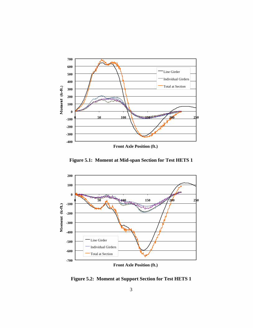
-400

-300

-200

-100

0

100

200

300

400

500

600

700

0 50 100 150 200 250

Front Axle Position (ft.)

Line Girder

Individual Girders

Total at Section

Figure 5.1: Moment at Mid-span Section for Test HETS 1

-700

-600

-500

-400

-300

-200

-100

0

100

200

0 50 100 150 200 250

Front Axle Position (ft.)

Line Girder

Individual Girders

Total at Section

Figure 5.2: Moment at Support Section for Test HETS 1

3

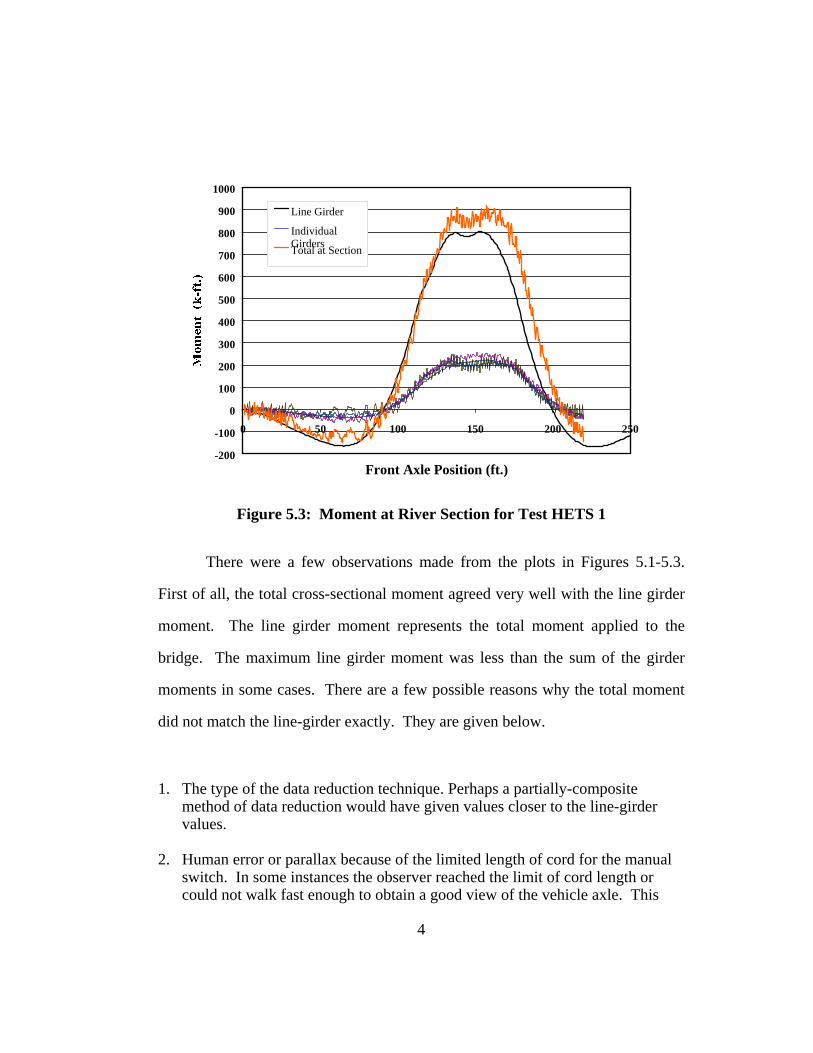
-200

-100

0

100

200

300

400

500

600

700

800

900

1000

0 50 100 150 200 250

Front Axle Position (ft.)

Line Girder

IndividualGirdersTotal at Section

Figure 5.3: Moment at River Section for Test HETS 1

There were a few observations made from the plots in Figures 5.1-5.3.

First of all, the total cross-sectional moment agreed very well with the line girder

moment. The line girder moment represents the total moment applied to the

bridge. The maximum line girder moment was less than the sum of the girder

moments in some cases. There are a few possible reasons why the total moment

did not match the line-girder exactly. They are given below.

1. The type of the data reduction technique. Perhaps a partially-composite

method of data reduction would have given values closer to the line-girder values.

2. Human error or parallax because of the limited length of cord for the manual

switch. In some instances the observer reached the limit of cord length or could not walk fast enough to obtain a good view of the vehicle axle. This

4

would have caused the data to be skewed with respect to the line girder moment.

3. Noise and oscillation in the data acquisition system caused by exterior radio

signals. 4. Moment carried by the slab that was not accounted for in spite of the data

reduction method used.

More significant observations with respect to the plots for a dump truck test are

given in Section 5.1.2.

5.1.2. Plots of Moment for a Complete Dump Truck Run

It was noted that the spacing between the individual moment histories for

each girder changed as the vehicle moved across the bridge. The girders directly

under the vehicles path carried a greater portion of the load when the vehicle is

near the section than when the vehicle was far from the section. This was most

evident in tests where the vehicle was not centered laterally on the bridge, such as

the dump truck tests.

Unfiltered moment histories from tests D.T. 1-2b and D.T. 3-4a are shown

in Figures 5.4-5.9. Girders 1 and 2 are shown in one color on the plots. Girders 3

and 4 are both shown in another. Recall that the D.T. 1-2b means that the dump

truck was located on the side of the bridge over girders 1 and 2., likewise with

D.T. 3-4a over girders 3 and 4. Since the truck positions were symmetric about

the bridge centerline, the values appear to be exactly reversed when looking at

both plots on a page at the same time. The values given for girders 1 and 2 in the

plots for D.T. 1-2b should match the values given for girders 3 and 4 in plots of

D.T. 3-4a.

5

Using Figures 5.4 and 5.5 as an example, the Mid-span moments found in

girders 1 and 2 for the D.T. 1-2 tests, and those found in girders 3 and 4 for the

D.T. 3-4 tests were markedly higher than the other two girders for vehicle

locations between 0’ and 70’ (in the same span as the instrumentation). The

values of moment in all girders at the Mid-span section became more equal to

each other when the vehicle moved into the next span (between 70’ and 160’).

The values of moment in all girders were practically equal in value by the time

the vehicle moved into the third span.

6

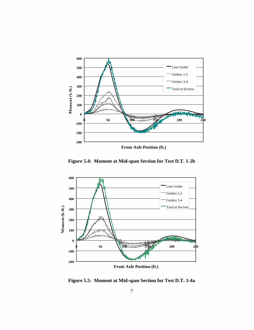
-300

-200

-100

0

100

200

300

400

500

600

0 50 100 150 200 250

Front Axle Position (ft.)

Line Girder

Girders 1-2

Girders 3-4

Total at Section

Figure 5.4: Moment at Mid-span Section for Test D.T. 1-2b

-200

-100

0

100

200

300

400

500

600

0 50 100 150 200 250

Front Axle Position (ft.)

Line Girder

Girders 1-2

Girders 3-4

Total at Section

Figure 5.5: Moment at Mid-span Section for Test D.T. 3-4a

7

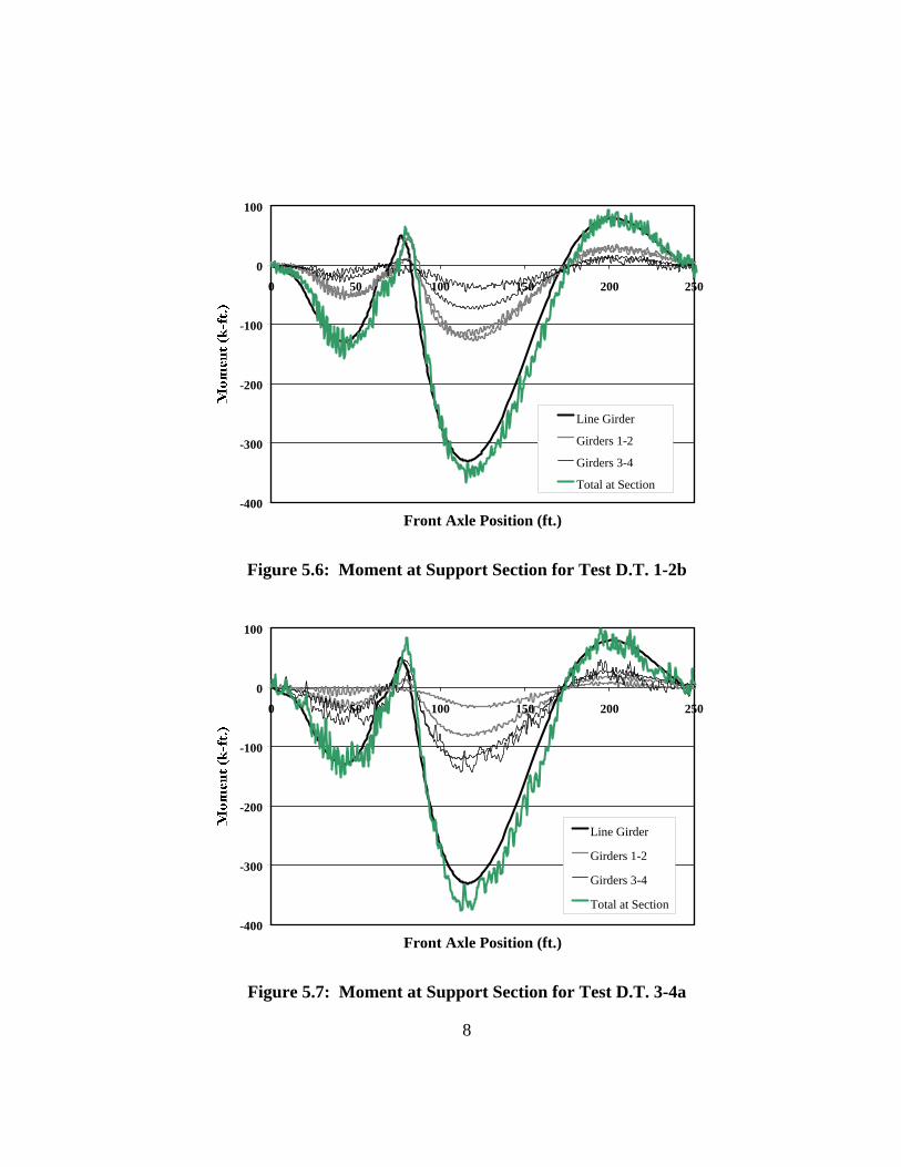
-400

-300

-200

-100

0

100

0 50 100 150 200 250

Front Axle Position (ft.)

Line Girder

Girders 1-2

Girders 3-4

Total at Section

Figure 5.6: Moment at Support Section for Test D.T. 1-2b

-400

-300

-200

-100

0

100

0 50 100 150 200 250

Front Axle Position (ft.)

Line Girder

Girders 1-2

Girders 3-4

Total at Section

Figure 5.7: Moment at Support Section for Test D.T. 3-4a

8

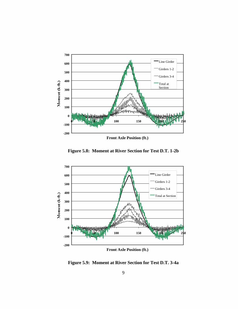
-200

-100

0

100

200

300

400

500

600

700

0 50 100 150 200 250

Front Axle Position (ft.)

Line Girder

Girders 1-2

Girders 3-4

Total atSection

Figure 5.8: Moment at River Section for Test D.T. 1-2b

-200

-100

0

100

200

300

400

500

600

700

0 50 100 150 200 250

Front Axle Position (ft.)

Line Girder

Girders 1-2

Girders 3-4

Total at Section

Figure 5.9: Moment at River Section for Test D.T. 3-4a

9

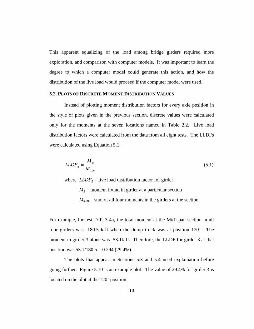
This apparent equalizing of the load among bridge girders required more

exploration, and comparison with computer models. It was important to learn the

degree to which a computer model could generate this action, and how the

distribution of the live load would proceed if the computer model were used.

5.2. PLOTS OF DISCRETE MOMENT DISTRIBUTION VALUES

Instead of plotting moment distribution factors for every axle position in

the style of plots given in the previous section, discrete values were calculated

only for the moments at the seven locations named in Table 2.2. Live load

distribution factors were calculated from the data from all eight tests. The LLDFs

were calculated using Equation 5.1.

sum

gg M

MLLDF = (5.1)

where LLDFg = live load distribution factor for girder

Mg = moment found in girder at a particular section

Msum = sum of all four moments in the girders at the section

For example, for test D.T. 3-4a, the total moment at the Mid-span section in all

four girders was -180.5 k-ft when the dump truck was at position 120’. The

moment in girder 3 alone was -53.1k-ft. Therefore, the LLDF for girder 3 at that

position was 53.1/180.5 = 0.294 (29.4%).

The plots that appear in Sections 5.3 and 5.4 need explaination before

going further. Figure 5.10 is an example plot. The value of 29.4% for girder 3 is

located on the plot at the 120’ position.

10

0

10

20

30

40

50

0 50 100 150 200

Position of Front Axle Along Bridge (ft.)

Girder 1 Girder 2 Girder 3 Girder 4 Supports Gaged Section

Figure 5.10: Example Moment Distribution Plot Taken From Test D.T.3-4a

The units of the abscissa are feet along bridge. Vertical lines connected by

hollow triangles show the locations of interior supports. Thus, these lines break

the plots into three spans, just like the actual bridge. There is also a line

indicating the location of the gauged section relative to the supports. The values

plotted on the ordinate indicate the percentage of the total moment at that section

that is found in each girder. Therefore, for any front axle position, the sum of all

four plotted points equals 100%.

5.3. DISCUSSION OF BRUFEM MODELING ISSUES

Before BRUFEM was used to obtain moment distribution estimates for

comparison to measured data, two inquiries were made with respect to BRUFEM

modeling. A comparison of the Eccentric Girder Model and the Composite

11

Girder Model was used to be sure that the choice of method had negligible impact

on moment distribution. Also, a study of the effect of diaphragms was needed in

order to see if they should be included in the BRUFEM model.

5.3.1. Comparison of EGM and CGM Methods

The BRUFEM modeling technique chosen for comparison was the CGM.

This was done because the CGM uses a method of calculation similar to the Fully

Composite method of data reduction. The EGM does not calculate values in the

same manner that the CGM does, but is supposed to yield greater accuracy

according to the BRUFEM manual. An investigation into the EGM was

appropriate in order to show that the differences between the EGM and CGM

were small. This validated the use of BRUFEM’s simpler modeling technique.

Figures 5.11 and 5.12 show selected moment distribution plots for a dump

truck and analysis performed in BRUFEM. The first plot shows the results using

the EGM method, and the other shows the CGM method. The figures shown are

representative of all of the test runs analyzed using both techniques. The plots are

almost identical.

12

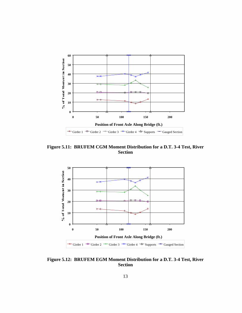
0

10

20

30

40

50

60

0 50 100 150 200

Position of Front Axle Along Bridge (ft.)

Girder 1 Girder 2 Girder 3 Girder 4 Supports Gauged Section

Figure 5.11: BRUFEM CGM Moment Distribution for a D.T. 3-4 Test, River Section

0

10

20

30

40

50

0 50 100 150 200

Position of Front Axle Along Bridge (ft.)

Girder 1 Girder 2 Girder 3 Girder 4 Supports Gauged Section

Figure 5.12: BRUFEM EGM Moment Distribution for a D.T. 3-4 Test, River Section

13

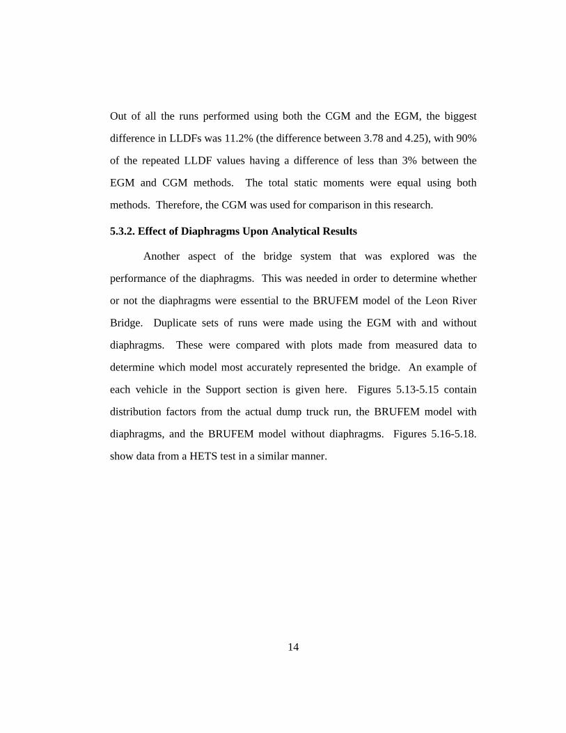
Out of all the runs performed using both the CGM and the EGM, the biggest

difference in LLDFs was 11.2% (the difference between 3.78 and 4.25), with 90%

of the repeated LLDF values having a difference of less than 3% between the

EGM and CGM methods. The total static moments were equal using both

methods. Therefore, the CGM was used for comparison in this research.

5.3.2. Effect of Diaphragms Upon Analytical Results

Another aspect of the bridge system that was explored was the

performance of the diaphragms. This was needed in order to determine whether

or not the diaphragms were essential to the BRUFEM model of the Leon River

Bridge. Duplicate sets of runs were made using the EGM with and without

diaphragms. These were compared with plots made from measured data to

determine which model most accurately represented the bridge. An example of

each vehicle in the Support section is given here. Figures 5.13-5.15 contain

distribution factors from the actual dump truck run, the BRUFEM model with

diaphragms, and the BRUFEM model without diaphragms. Figures 5.16-5.18.

show data from a HETS test in a similar manner.

14

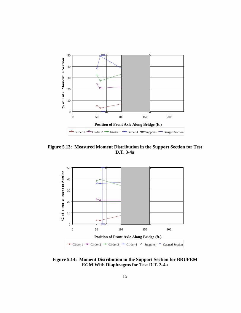
0

10

20

30

40

50

0 50 100 150 200

Position of Front Axle Along Bridge (ft.)

Girder 1 Girder 2 Girder 3 Girder 4 Supports Gauged Section

Figure 5.13: Measured Moment Distribution in the Support Section for Test D.T. 3-4a

0

10

20

30

40

50

0 50 100 150 200

Position of Front Axle Along Bridge (ft.)

Girder 1 Girder 2 Girder 3 Girder 4 Supports Gauged Section

Figure 5.14: Moment Distribution in the Support Section for BRUFEM EGM With Diaphragms for Test D.T. 3-4a

15

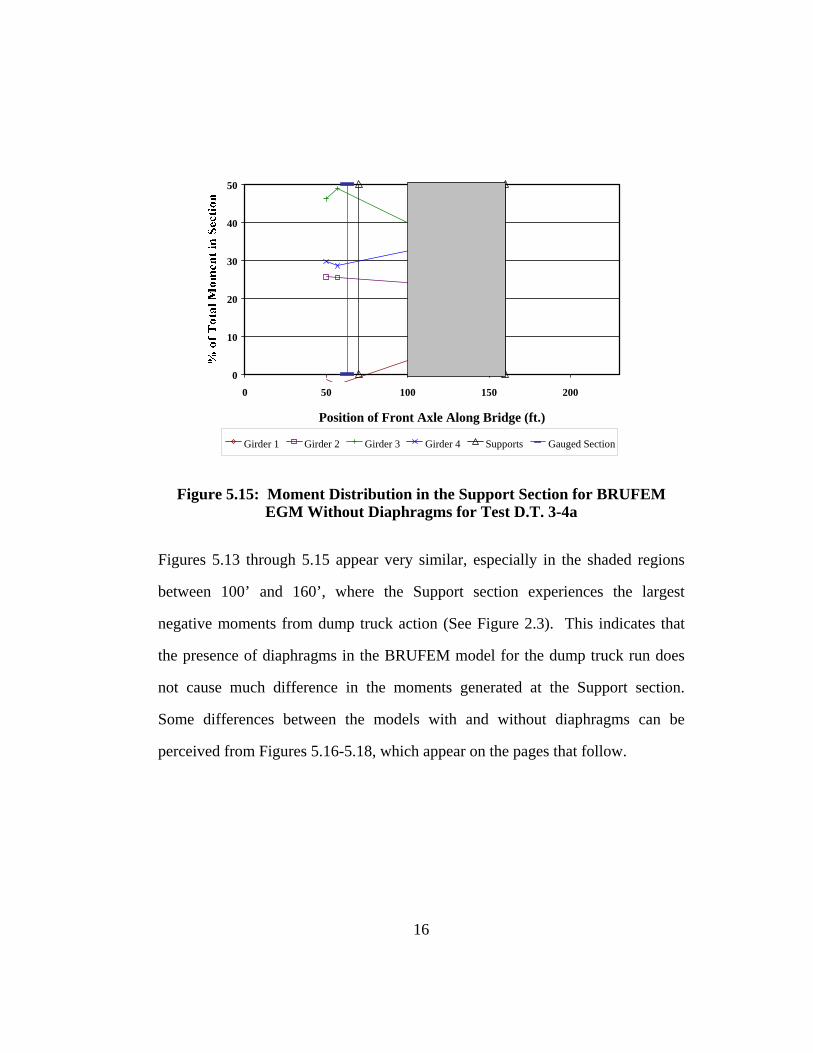
0

10

20

30

40

50

0 50 100 150 200

Position of Front Axle Along Bridge (ft.)

Girder 1 Girder 2 Girder 3 Girder 4 Supports Gauged Section

Figure 5.15: Moment Distribution in the Support Section for BRUFEM EGM Without Diaphragms for Test D.T. 3-4a

Figures 5.13 through 5.15 appear very similar, especially in the shaded regions

between 100’ and 160’, where the Support section experiences the largest

negative moments from dump truck action (See Figure 2.3). This indicates that

the presence of diaphragms in the BRUFEM model for the dump truck run does

not cause much difference in the moments generated at the Support section.

Some differences between the models with and without diaphragms can be

perceived from Figures 5.16-5.18, which appear on the pages that follow.

16

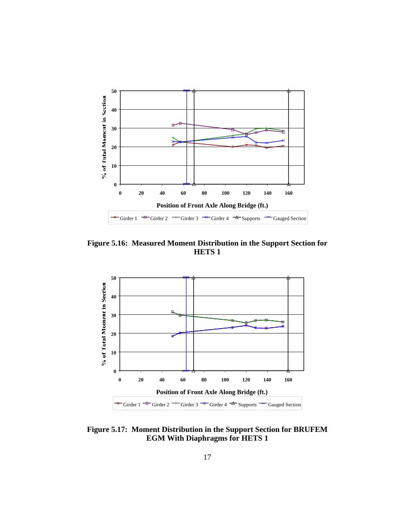
0

10

20

30

40

50

0 20 40 60 80 100 120 140 160

Position of Front Axle Along Bridge (ft.)

Girder 1 Girder 2 Girder 3 Girder 4 Supports Gauged Section

Figure 5.16: Measured Moment Distribution in the Support Section for HETS 1

0

10

20

30

40

50

0 20 40 60 80 100 120 140 160

Position of Front Axle Along Bridge (ft.)

Girder 1 Girder 2 Girder 3 Girder 4 Supports Gauged Section

Figure 5.17: Moment Distribution in the Support Section for BRUFEM EGM With Diaphragms for HETS 1

17

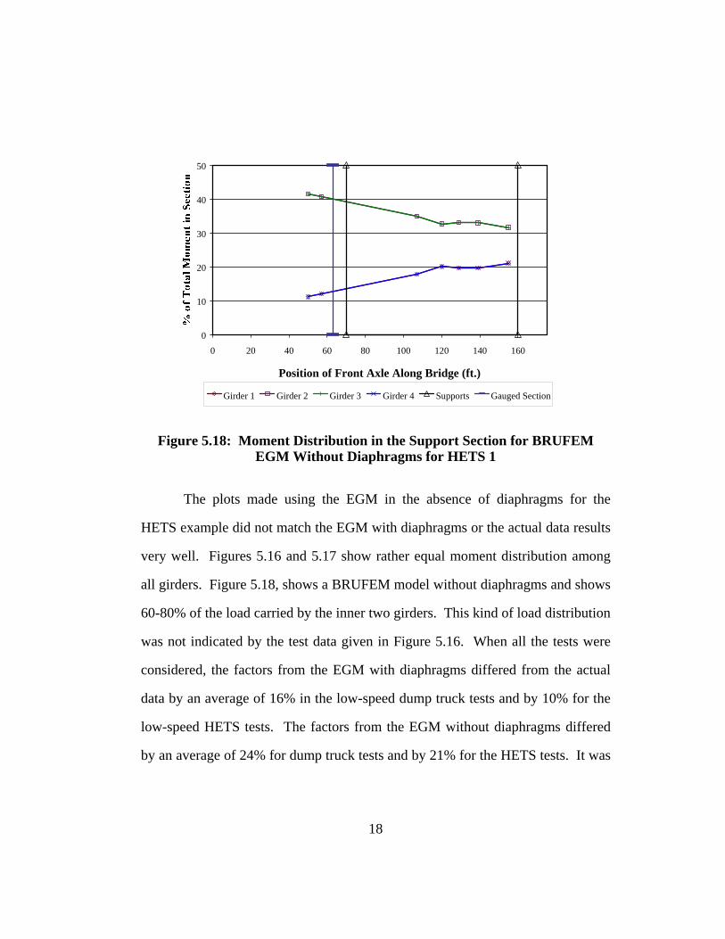
0

10

20

30

40

50

0 20 40 60 80 100 120 140 160

Position of Front Axle Along Bridge (ft.)

Girder 1 Girder 2 Girder 3 Girder 4 Supports Gauged Section

Figure 5.18: Moment Distribution in the Support Section for BRUFEM EGM Without Diaphragms for HETS 1

The plots made using the EGM in the absence of diaphragms for the

HETS example did not match the EGM with diaphragms or the actual data results

very well. Figures 5.16 and 5.17 show rather equal moment distribution among

all girders. Figure 5.18, shows a BRUFEM model without diaphragms and shows

60-80% of the load carried by the inner two girders. This kind of load distribution

was not indicated by the test data given in Figure 5.16. When all the tests were

considered, the factors from the EGM with diaphragms differed from the actual

data by an average of 16% in the low-speed dump truck tests and by 10% for the

low-speed HETS tests. The factors from the EGM without diaphragms differed

by an average of 24% for dump truck tests and by 21% for the HETS tests. It was

18

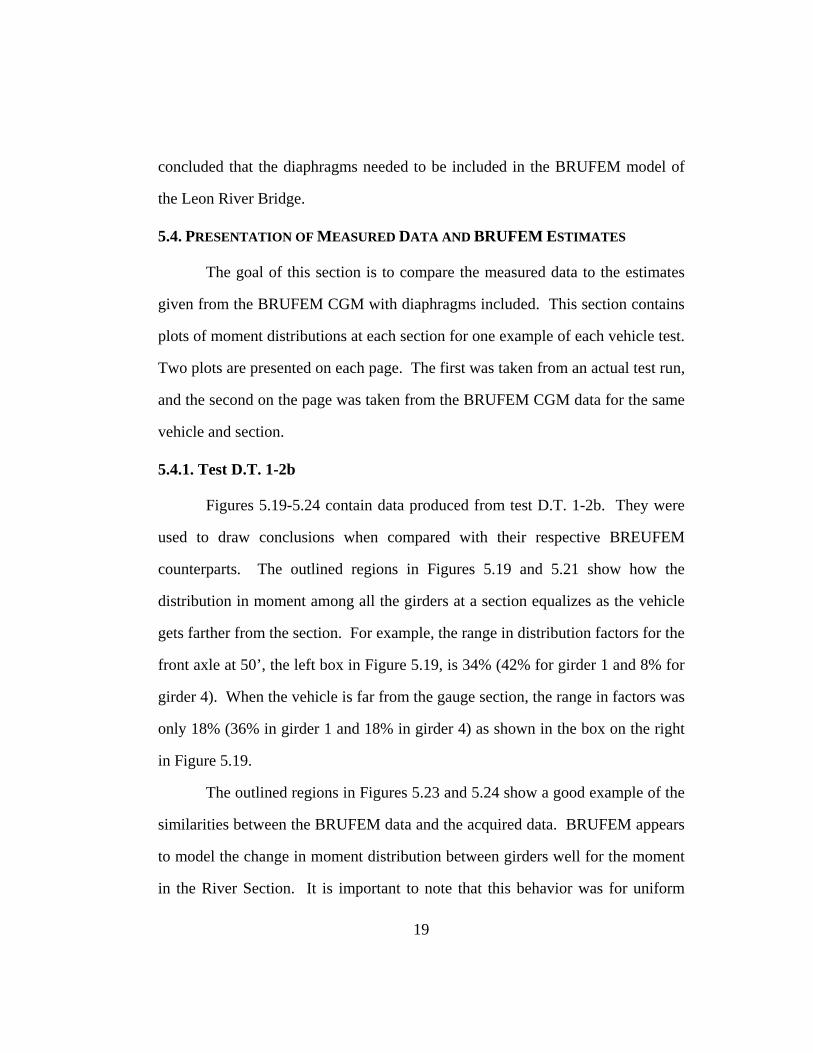
concluded that the diaphragms needed to be included in the BRUFEM model of

the Leon River Bridge.

5.4. PRESENTATION OF MEASURED DATA AND BRUFEM ESTIMATES

The goal of this section is to compare the measured data to the estimates

given from the BRUFEM CGM with diaphragms included. This section contains

plots of moment distributions at each section for one example of each vehicle test.

Two plots are presented on each page. The first was taken from an actual test run,

and the second on the page was taken from the BRUFEM CGM data for the same

vehicle and section.

5.4.1. Test D.T. 1-2b

Figures 5.19-5.24 contain data produced from test D.T. 1-2b. They were

used to draw conclusions when compared with their respective BREUFEM

counterparts. The outlined regions in Figures 5.19 and 5.21 show how the

distribution in moment among all the girders at a section equalizes as the vehicle

gets farther from the section. For example, the range in distribution factors for the

front axle at 50’, the left box in Figure 5.19, is 34% (42% for girder 1 and 8% for

girder 4). When the vehicle is far from the gauge section, the range in factors was

only 18% (36% in girder 1 and 18% in girder 4) as shown in the box on the right

in Figure 5.19.

The outlined regions in Figures 5.23 and 5.24 show a good example of the

similarities between the BRUFEM data and the acquired data. BRUFEM appears

to model the change in moment distribution between girders well for the moment

in the River Section. It is important to note that this behavior was for uniform

19

action in which the truck was always in the center span. Figures 5.19 to 5.24 are

given on the pages that follow.

20

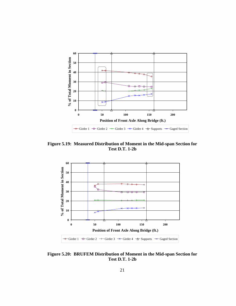
0

10

20

30

40

50

60

0 50 100 150 200

Position of Front Axle Along Bridge (ft.)

% o

f Tot

al M

omen

t in

Sect

ion

Girder 1 Girder 2 Girder 3 Girder 4 Supports Gaged Section

Figure 5.19: Measured Distribution of Moment in the Mid-span Section for Test D.T. 1-2b

0

10

20

30

40

50

60

0 50 100 150 200

Position of Front Axle Along Bridge (ft.)

% o

f Tot

al M

omen

t in

Sect

ion

Girder 1 Girder 2 Girder 3 Girder 4 Supports Gaged Section

Figure 5.20: BRUFEM Distribution of Moment in the Mid-span Section for Test D.T. 1-2b

21

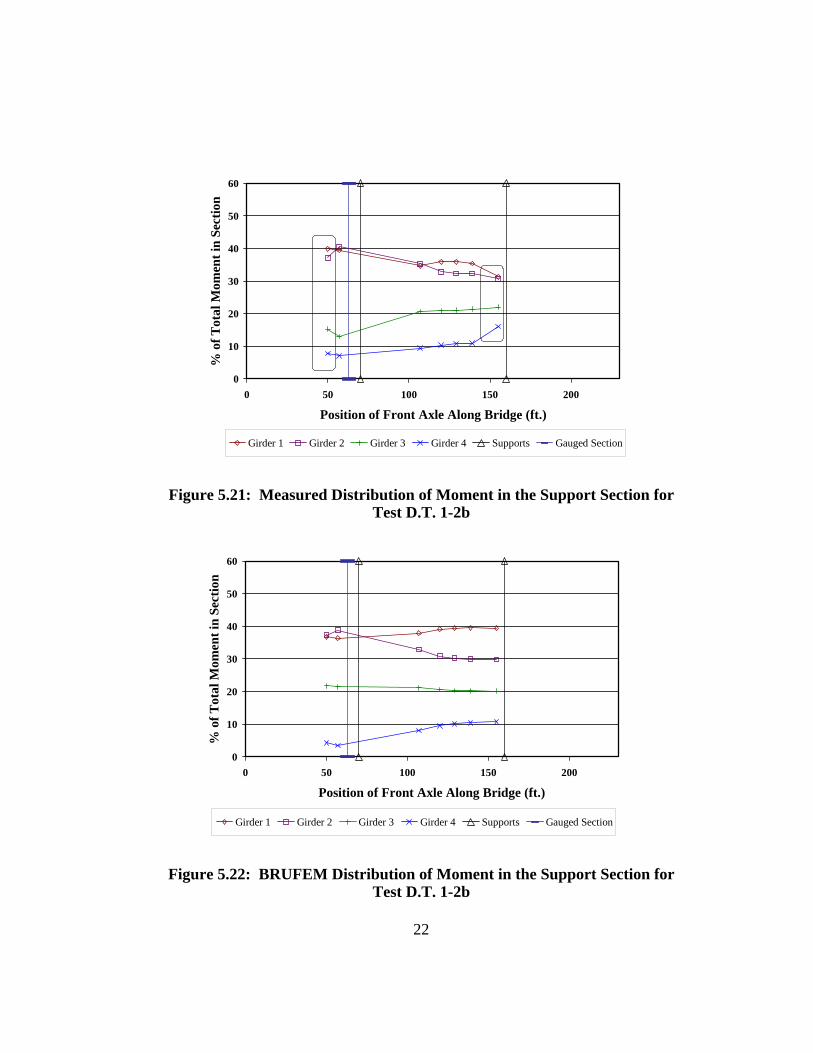
0

10

20

30

40

50

60

0 50 100 150 200

Position of Front Axle Along Bridge (ft.)

% o

f Tot

al M

omen

t in

Sect

ion

Girder 1 Girder 2 Girder 3 Girder 4 Supports Gauged Section

Figure 5.21: Measured Distribution of Moment in the Support Section for Test D.T. 1-2b

0

10

20

30

40

50

60

0 50 100 150 200

Position of Front Axle Along Bridge (ft.)

% o

f Tot

al M

omen

t in

Sect

ion

Girder 1 Girder 2 Girder 3 Girder 4 Supports Gauged Section

Figure 5.22: BRUFEM Distribution of Moment in the Support Section for Test D.T. 1-2b

22

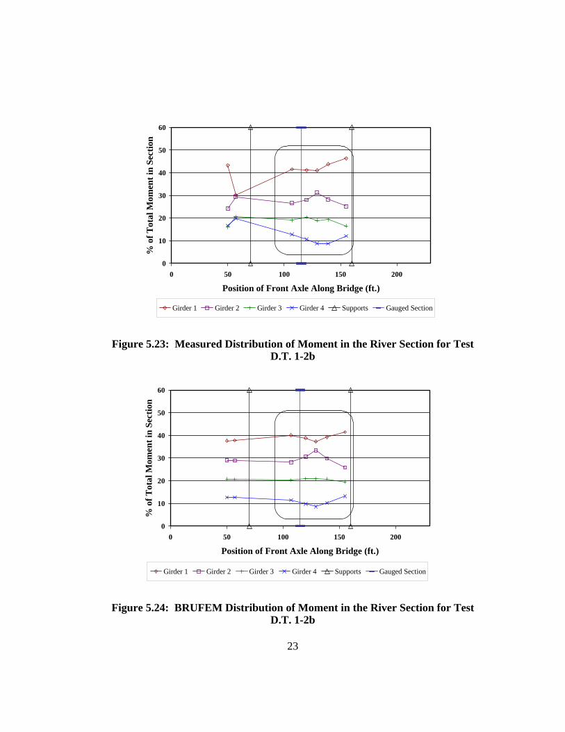
0

10

20

30

40

50

60

0 50 100 150 200

Position of Front Axle Along Bridge (ft.)

% o

f Tot

al M

omen

t in

Sect

ion

Girder 1 Girder 2 Girder 3 Girder 4 Supports Gauged Section

Figure 5.23: Measured Distribution of Moment in the River Section for Test D.T. 1-2b

0

10

20

30

40

50

60

0 50 100 150 200

Position of Front Axle Along Bridge (ft.)

% o

f Tot

al M

omen

t in

Sect

ion

Girder 1 Girder 2 Girder 3 Girder 4 Supports Gauged Section

Figure 5.24: BRUFEM Distribution of Moment in the River Section for Test D.T. 1-2b

23

5.4.2. Test HETS 2

The next six figures give plots for the HETS 2 test in the same format as

those given in Section 5.4.2. The distribution of load across the bridge section

was more uniform since the HETS vehicle was aligned on the bridge centerline.

Most LLDFs for all girders were bounded between 20% and 30%. Notice that the

BRUFEM values for girders 1 and 4 and the values for girders 2 and 3 are equal

due to this symmetry. The effect of load distribution with vehicle distance was

not seen easily in these plots. These plots do show the good correlation between

the acquired data and BRUFEM model data.

24

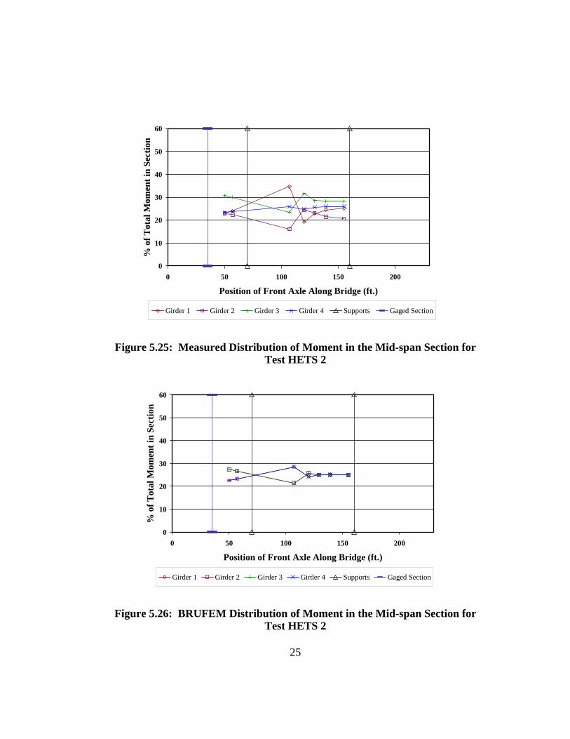
0

10

20

30

40

50

60

0 50 100 150 200

Position of Front Axle Along Bridge (ft.)

% o

f Tot

al M

omen

t in

Sect

ion

Girder 1 Girder 2 Girder 3 Girder 4 Supports Gaged Section

Figure 5.25: Measured Distribution of Moment in the Mid-span Section for Test HETS 2

0

10

20

30

40

50

60

0 50 100 150 200

Position of Front Axle Along Bridge (ft.)

% o

f Tot

al M

omen

t in

Sect

ion

Girder 1 Girder 2 Girder 3 Girder 4 Supports Gaged Section

Figure 5.26: BRUFEM Distribution of Moment in the Mid-span Section for Test HETS 2

25

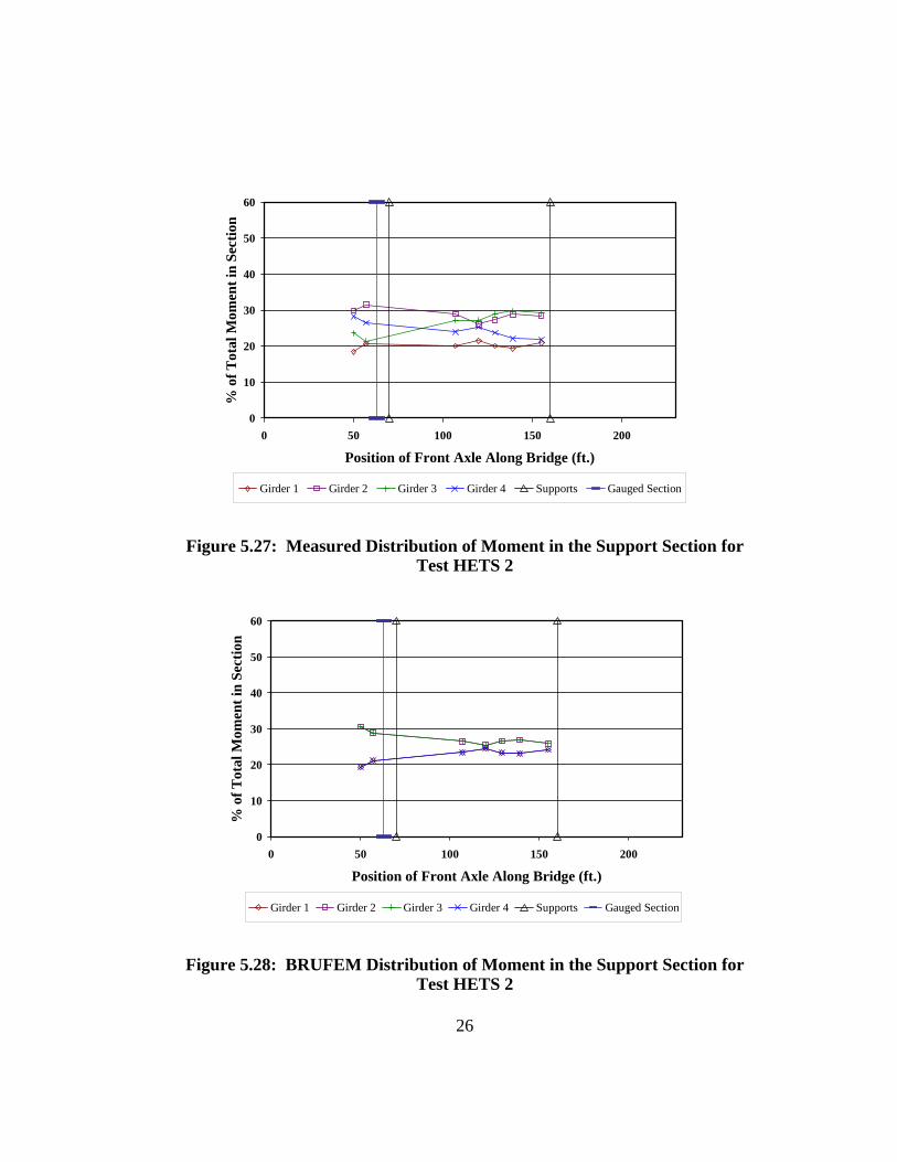
0

10

20

30

40

50

60

0 50 100 150 200

Position of Front Axle Along Bridge (ft.)

% o

f Tot

al M

omen

t in

Sect

ion

Girder 1 Girder 2 Girder 3 Girder 4 Supports Gauged Section

Figure 5.27: Measured Distribution of Moment in the Support Section for Test HETS 2

0

10

20

30

40

50

60

0 50 100 150 200

Position of Front Axle Along Bridge (ft.)

% o

f Tot

al M

omen

t in

Sect

ion

Girder 1 Girder 2 Girder 3 Girder 4 Supports Gauged Section

Figure 5.28: BRUFEM Distribution of Moment in the Support Section for Test HETS 2

26

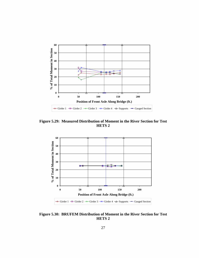
0

10

20

30

40

50

60

0 50 100 150 200

Position of Front Axle Along Bridge (ft.)

% o

f Tot

al M

omen

t in

Sect

ion

Girder 1 Girder 2 Girder 3 Girder 4 Supports Gauged Section

Figure 5.29: Measured Distribution of Moment in the River Section for Test HETS 2

0

10

20

30

40

50

60

0 50 100 150 200

Position of Front Axle Along Bridge (ft.)

% o

f Tot

al M

omen

t in

Sect

ion

Girder 1 Girder 2 Girder 3 Girder 4 Supports Gauged Section

Figure 5.30: BRUFEM Distribution of Moment in the River Section for Test HETS 2

27

28

Overall, Figures 5.19-5.30 show very good correlation between the test

data and BRUFEM predictions. The plots for dump truck action in Figures 5.19-

5.24 show good results for the relationship between all four girders with a

asymmetric loading. All the plots for the HETS shown in Figures 5.25-5.30 show

fairly equal sharing of the load for the overweight vehicle on the center of the

bridge.

Chapter 6: Design Live Load Distribution Factors

The acquired test data compared well with the output from BRUFEM.

The next step was to compare the reduced data with the lateral load distribution

factors found in the old AASHTO Working Stress Design (WSD) code and the

new AASHTO LRFD code. Lateral load distribution factors for all sections were

obtained for the vehicle positions of interest. The AASHTO LRFD design code

contains a combination of empirical equations, approximate formulas, and special

analysis techniques to determine live load distribution factors for use in design.

The AASHTO WSD code contains a simpler equation for deriving LLDFs. These

were utilized in order to see how well the design methods match what was

obtained in the field.

6.1. METHOD FOR CALCULATING LLDFS

LLDFs from the test data and design codes were calculated in different

ways. A single equation was used in the case of the actual data. Design LLDFs

were found using a range of equations depending of the geometry and location of

the girder. Also, the LLDFs from the test data were calculated only at the vehicle

positions of interest, whereas the design LLDFs were applied to any vehicle

location.

6.1.1. LLDFs from Test Data

Live load distribution factors were calculated from the data from all eight

tests. The LLDFs were calculated using Equation 5.1 given previously in Section

5.2. Note that that method does not divide the moment in one girder by the line

1

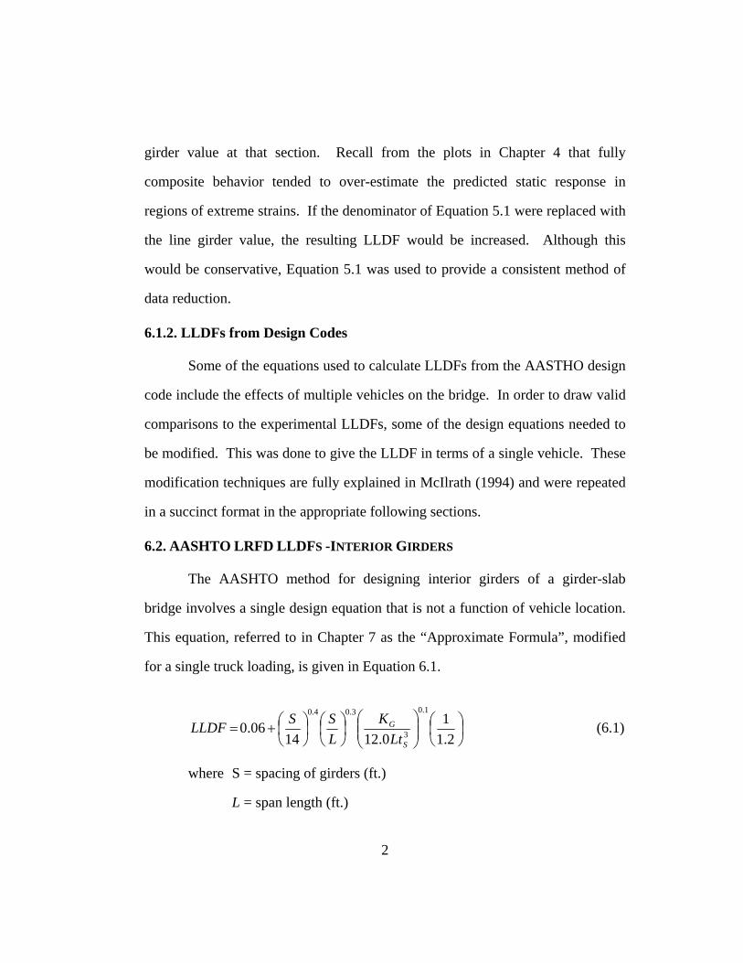
girder value at that section. Recall from the plots in Chapter 4 that fully

composite behavior tended to over-estimate the predicted static response in

regions of extreme strains. If the denominator of Equation 5.1 were replaced with

the line girder value, the resulting LLDF would be increased. Although this

would be conservative, Equation 5.1 was used to provide a consistent method of

data reduction.

6.1.2. LLDFs from Design Codes

Some of the equations used to calculate LLDFs from the AASTHO design

code include the effects of multiple vehicles on the bridge. In order to draw valid

comparisons to the experimental LLDFs, some of the design equations needed to

be modified. This was done to give the LLDF in terms of a single vehicle. These

modification techniques are fully explained in McIlrath (1994) and were repeated

in a succinct format in the appropriate following sections.

6.2. AASHTO LRFD LLDFS -INTERIOR GIRDERS

The AASHTO method for designing interior girders of a girder-slab

bridge involves a single design equation that is not a function of vehicle location.

This equation, referred to in Chapter 7 as the “Approximate Formula”, modified

for a single truck loading, is given in Equation 6.1.

⎟⎠⎞

⎜⎝⎛

⎟⎟⎠

⎞⎜⎜⎝

⎛⎟⎠⎞

⎜⎝⎛

⎟⎠⎞

⎜⎝⎛+=

2.11

0.121406.0

1.0

3

3.04.0

S

G

LtK

LSSLLDF (6.1)

where S = spacing of girders (ft.)

L = span length (ft.)

2

Kg = longitudinal stiffness parameter

ts = thickness of the deck slab (in.)

( )2

gG AeInK +⋅= (6.2)

where n = the modular ratio of steel to concrete = 7.25

I = moment of inertia of girder (in4)

A = cross-sectional area of girder (in2)

eg = distance between the centers of gravity of the girder alone and

deck slab alone (in.)

Equation 6.1 is valid for loading of one design lane in the category of bridges that

includes the Leon River Bridge. This AASHTO equation has a built-in Multiple

Presence Factor. The factor of (1/1.2) was applied to eliminate this effect and

give a LLDF in terms of a single vehicle. The use of Equation 6.1 was only valid

if the variables involved meet the range of applicability given in the AASHTO

code. The bridge must have at least four girders and fulfill the other requirements

given below.

0.165.3 ≤≤ S

24020 ≤≤ L

0.125.4 ≤≤ st

000,000,7000,10 ≤≤ GK

The Leon River Bridge fulfilled all of these requirements.

3

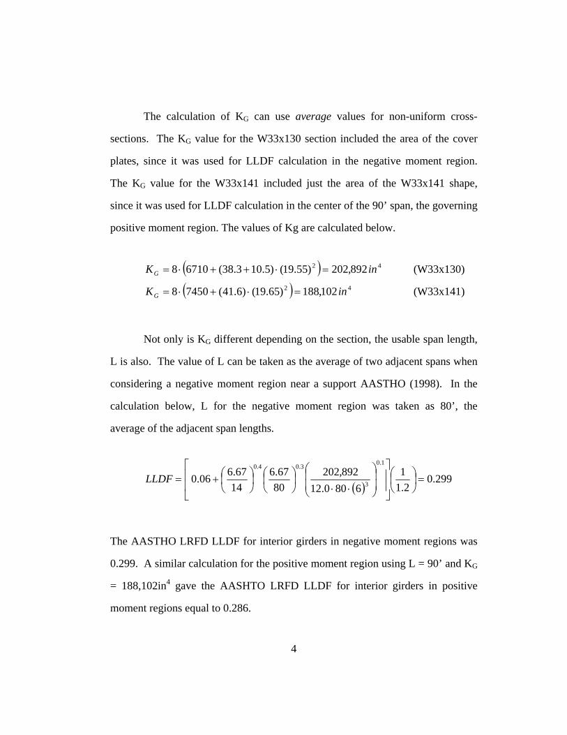
The calculation of KG can use average values for non-uniform cross-

sections. The KG value for the W33x130 section included the area of the cover

plates, since it was used for LLDF calculation in the negative moment region.

The KG value for the W33x141 included just the area of the W33x141 shape,

since it was used for LLDF calculation in the center of the 90’ span, the governing

positive moment region. The values of Kg are calculated below.

( ) 42 892,202)55.19()5.103.38(67108 inKG =⋅++⋅= (W33x130)

( ) 42 102,188)65.19()6.41(74508 inKG =⋅+⋅= (W33x141)

Not only is KG different depending on the section, the usable span length,

L is also. The value of L can be taken as the average of two adjacent spans when

considering a negative moment region near a support AASTHO (1998). In the

calculation below, L for the negative moment region was taken as 80’, the

average of the adjacent span lengths.

( )299.0

2.11

6800.12892,202

8067.6

1467.606.0

1.0

3

3.04.0

=⎟⎠⎞

⎜⎝⎛⎥⎥

⎦

⎤

⎢⎢

⎣

⎡

⎟⎟

⎠

⎞

⎜⎜

⎝

⎛

⋅⋅⎟⎠⎞

⎜⎝⎛

⎟⎠⎞

⎜⎝⎛+=LLDF

The AASTHO LRFD LLDF for interior girders in negative moment regions was

0.299. A similar calculation for the positive moment region using L = 90’ and KG

= 188,102in4 gave the AASHTO LRFD LLDF for interior girders in positive

moment regions equal to 0.286.

4

6.3. AASHTO LRFD LLDFS - EXTERIOR GIRDERS

The Leon River Bridge is a zero-skew bridge with a cast-in-place deck on

steel girders. AASHTO has three major methods for the design of the exterior

girder for bridges of this type. The distribution of moment in the exterior girders

is approximated by either the “lever rule,” a method of rigid body analysis, or a

factored version of the equation for interior girders.

6.3.1. Lever Rule

The lever rule is a method that uses statics alone to determine the

distribution of load to the exterior girder of the bridge. The method assumes that

a hinge is located at the next innermost girder. A summation of moments using

this zero-moment location was used to determine the portion of the vehicle load,

T, supported by the exterior girder. The reaction by the exterior girder was given

as R. The value of R/T is the LLDF for the exterior girder. This was done for

two different locations for each vehicle, the actual position and the AASTHO

design case.

AASHTO requires that the vehicle be placed with its wheels no closer

than 24” to the curb. This serves to give the largest and safest LLDF for design of

exterior girders. The vehicle was also placed in the same lateral position that it

was during the actual test. This does not give the worst possible LLDF, but was

done to get a LLDF for comparison to the actual test data. The AASHTO and

actual axle locations for the dump truck are shown in Figures 6.1 and 6.2. The

5

AASHTO and actual axle locations for HETS are shown in Figures 6.3 and 6.4

respectively.

0.5 T0.5 T

8"80"

80"

24"

Assumed Hinge

Figure 6.1: AASHTO Lever Rule Dump Truck Position

R

0.5 T

43.6"

80"

Assumed Hinge

Figure 6.2: Actual Dump Truck Lateral Position

6

R

0.25 T 0.25 T

48"80"

80"

24"

Assumed Hinge

Figure 6.3: AASHTO Lever Rule HETS Vehicle Position

0.25 T

R

22"

Assumed Hinge

80"

Figure 6.4: Actual HETS Vehicle Lateral Position

7

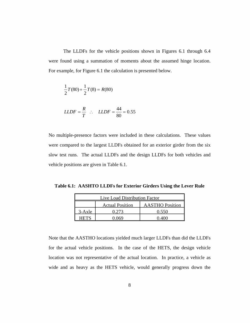
The LLDFs for the vehicle positions shown in Figures 6.1 through 6.4

were found using a summation of moments about the assumed hinge location.

For example, for Figure 6.1 the calculation is presented below.

)80()8(21)80(

21 RTT =+

55.08044

==∴= LLDFTRLLDF

No multiple-presence factors were included in these calculations. These values

were compared to the largest LLDFs obtained for an exterior girder from the six

slow test runs. The actual LLDFs and the design LLDFs for both vehicles and

vehicle positions are given in Table 6.1.

Table 6.1: AASHTO LLDFs for Exterior Girders Using the Lever Rule

Actual Position AASTHO Position3-Axle 0.273 0.550HETS 0.069 0.400

Live Load Distribution Factor

Note that the AASTHO locations yielded much larger LLDFs than did the LLDFs

for the actual vehicle positions. In the case of the HETS, the design vehicle

location was not representative of the actual location. In practice, a vehicle as

wide and as heavy as the HETS vehicle, would generally progress down the

8

longitudinal center of the bridge. Thus, the AASHTO LLDF was conservative by

a factor of 0.4/0.069 = 5.8 over the LLDF for the likely position of such an

overweight vehicle.

6.3.2. Rigid Body Analysis

Another way AASHTO permits LLDF calculation for the exterior girders

is by a rigid body analysis. In this method, the entire cross-section is assumed to

rotate about the longitudinal centerline of the bridge. The design vehicles were

placed at the same design locations required by AASTHO (24” from the curb) and

at the actual lateral locations used in the test runs. Equation 6.3 is the governing

equation for this method.

∑∑+=

b

L

N

Next

b

L

x

eXNNLLDF

12

1 (6.3)

where NL = number of loaded lanes under consideration

Nb = total number beams

e = eccentricity of a lane from the center of gravity of the pattern

of girders (ft.)

x = horizontal distance from the center of gravity of the pattern of

girders to each girder (ft.)

Xext = horizontal distance from the center of gravity of the pattern

of girders to the exterior girder (ft.)

The wheel locations and important dimensions for the dump truck and HETS

loading are shown in Figures 6.5 through 6.8.

9

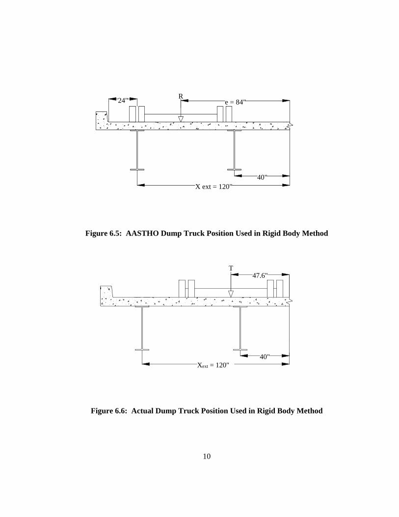
R24" e = 84"

40"X ext = 120"

Figure 6.5: AASTHO Dump Truck Position Used in Rigid Body Method

T 47.6"

Xext = 120" 40"

Figure 6.6: Actual Dump Truck Position Used in Rigid Body Method

10

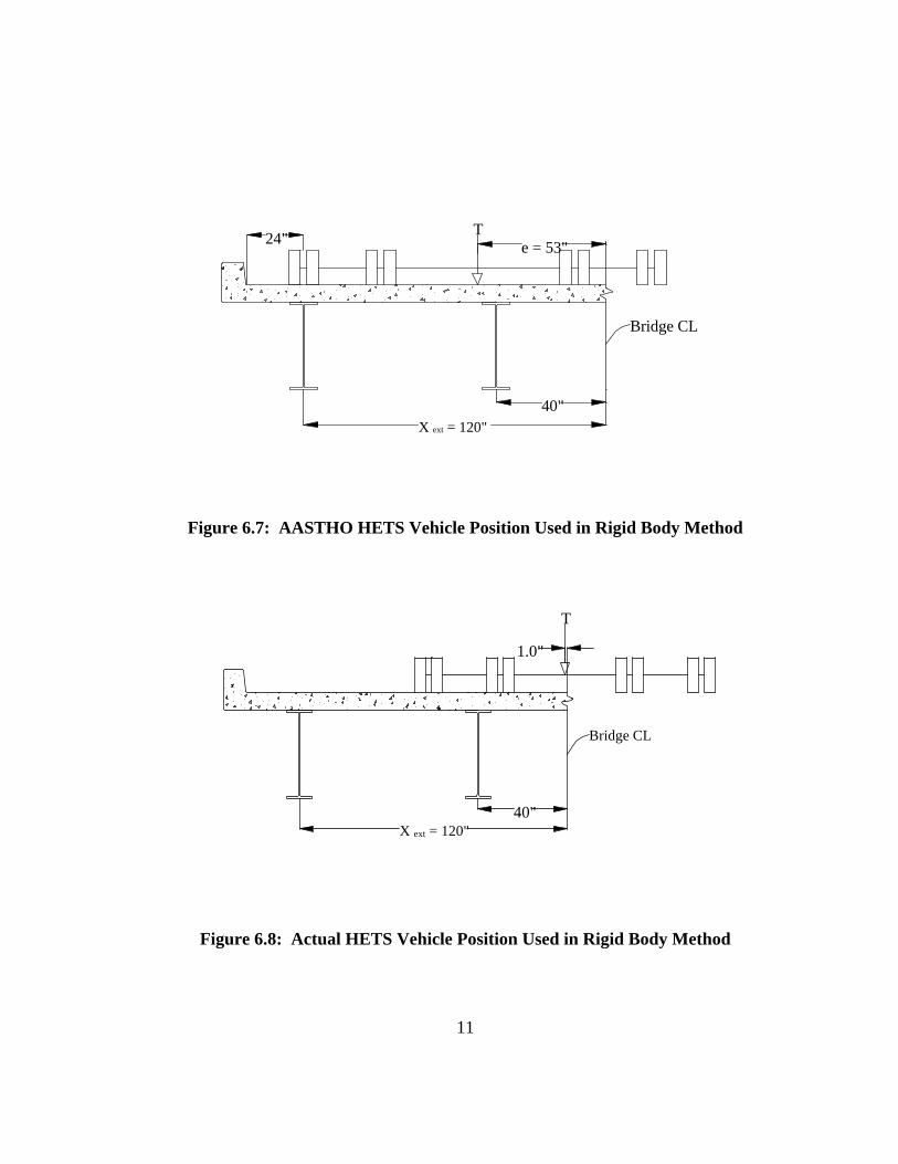
T24"

40"

e = 53"

X ext = 120"

Bridge CL

Figure 6.7: AASTHO HETS Vehicle Position Used in Rigid Body Method

Bridge CL

T

1.0"

40"X ext = 120"

Figure 6.8: Actual HETS Vehicle Position Used in Rigid Body Method

11

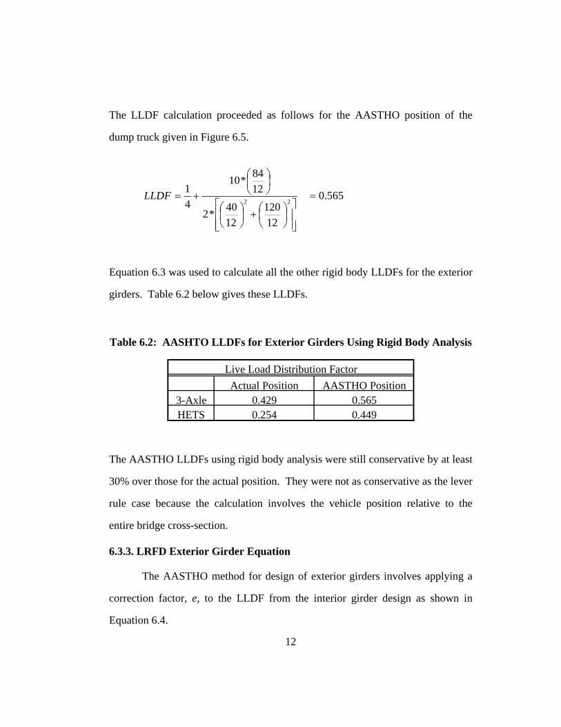
The LLDF calculation proceeded as follows for the AASTHO position of the

dump truck given in Figure 6.5.

565.0

12120

1240*2

1284*10

41

22=

⎥⎥⎦

⎤

⎢⎢⎣

⎡⎟⎠⎞

⎜⎝⎛+⎟

⎠⎞

⎜⎝⎛

⎟⎠⎞

⎜⎝⎛

+=LLDF

Equation 6.3 was used to calculate all the other rigid body LLDFs for the exterior

girders. Table 6.2 below gives these LLDFs.

Table 6.2: AASHTO LLDFs for Exterior Girders Using Rigid Body Analysis

Actual Position AASTHO Position3-Axle 0.429 0.565HETS 0.254 0.449

Live Load Distribution Factor

The AASTHO LLDFs using rigid body analysis were still conservative by at least

30% over those for the actual position. They were not as conservative as the lever

rule case because the calculation involves the vehicle position relative to the

entire bridge cross-section.

6.3.3. LRFD Exterior Girder Equation

The AASTHO method for design of exterior girders involves applying a

correction factor, e, to the LLDF from the interior girder design as shown in

Equation 6.4.

12

( ) ( )ExteriorInterior LLDFeLLDF *= (6.4)

The correction factor e is a function of de, which is the distance from the center of

the exterior girder to the beginning of the curb. This correction factor is given in

Equation 6.5.

0.11.9

77.0 ≥+= ede (6.5)

where e = correction factor

de = the distance between the center of the exterior beam and the

interior edge of the curb (ft)

Equation 6.6 is applicable only if de is between -1.0 and 5.5ft. The value of de for

the Leon River Bridge from Figure 1.8 was 2ft. Therefore, the correction factor

was 0.99 and taken as 1.0 according to Equation 6.5. In this case the LLDFs for

the exterior girders are the same as those for the interior girders. The LLDF

values were calculated in Section 6.2 and were 0.299 for negative moment regions

and 0.286 for positive moment regions.

6.4. LLDFS FROM THE AASHTO WORKING STRESS DESIGN CODE

The empirical equations using the AASTHO LLDFs from the Working

Stress Design code are simple. Depending on the number of lanes considered,

either of two equations is used. Since a single truck load was used in the field

13

tests, the equation for a single lane was used for comparison. Equation 6.6 from

the AASHTO WSD specification is given below.

( )7SLaneDesignOneLLDFLoadWheel = (6.6)

where: S = girder spacing = 6.67ft

Equation 6.6 is in terms of wheel loads. Since the distribution factors given in

this research were in terms of full vehicle loads, (in the same manner that the line

girders were loaded with full axles), Equation 6.6 needed also to be given in terms

of full axles. Therefore, a factor of 0.5 was applied to the above equation, which

yielded Equation 6.7.

( )14SLaneDesignOneLLDFLoadTruck = (6.7)

For the Leon River Bridge, S was equal to 6.67ft. Therefore the AASTHO WSD

LLDF was 6.67/14 = 0.476. This factor only depends on the girder spacing, and

therefore was valid in this research for both vehicles in positive and negative

moment regions.

14

Chapter 7: Comparison of Lateral Load Distribution Factors and Girder Moments

This chapter compares the LLDFs and design moments calculated from

the field data, from the BRUFEM model, and from various design codes. Three

criteria were used to organize the data. They were the type of load vehicle (dump

truck or HETS), type of girder (interior or exterior), and moment region (negative

or positive). A brief discussion of vehicle location is given before the LLDF data

tables are presented. Trends in the LLDFs and design moments are summarized

in the last section of this chapter.

7.1. LOCATIONS OF MAXIMUM STATIC RESPONSES

In Section 2.2.3 of this research, seven representative vehicle locations

were selected. Six of those locations were chosen because they were close to

extremes anticipated by the line girder analysis. However, the location of the

vehicle that gives the maximum response may have been a few feet from the

selected representative location. For example, one location for consideration was

139’ when the absolute maximum response was given at 141’ for the HETS.

Small differences in distance were neglected, since none of the selected locations

were farther than 4’ from a location of expected maximum moment. Table 2.1

gave a summary of the extreme values of moment taken from the line girder plots

of Chapter 2. All of the design LLDFs found in the next section were multiplied

to the maximum moment values in Table 2.1 in order to obtain design moment

values for comparison. For example, the maximum negative moment for the

1

dump truck was -331k-ft. Applying the AASTHO lever rule LLDF of 0.550 gave

a design moment of -331*0.55 = -182k-ft.

The dump truck values in Tables 7.5 and 7.7 contain two very different

truck positions for maximum moment for repeated tests. There is a simple

explanation for this. In the case of Table 7.5, the predicted static negative

moments in the support section when the truck was at 107’ and at 120’ were

-312k-ft and –325k-ft respectively. This is shown in Figure 2.4. Therefore, small

changes in moment in the girders caused governing moments in Table 7.5 to come

from either dump truck location. In the case of Table 7.7, Figures 2.3 and 2.5

show that the static moment in the Mid-span section for the dump truck at 50’ is

only about 60k-ft from the value given at the River section for a dump truck

location at 129’ (535k-ft compared with 593k-ft). Small changes in distribution

among girders caused some governing positive moments to come from either

section.

7.2. COMPARISON OF ACTUAL AND DESIGN LLDFS AND MOMENTS

This section presents the results of all the LLDF calculations done

throughout the course of this research. It also shows comparisons in terms of

design moment. In the tables that follow, values from the measured data are

given in the top portion. The values are averages from all the tests that involved

the same vehicle and lateral location on the bridge. The analysis and design

values are given in the lower portion. A moment value from design tools such as

BRUFEM or AASTHO LRFD was shown in bold type when it was

unconservative with respect to any test value in the same category.

2

In the following tables, five different entries are given for the AASTHO

LRFD design code. In summary, Equations 6.1 and 6.4 gave the “Approximate

Formula”. The “Lever Rule” for both positions was described in Section 6.3.1.

The “Rigid Body” method is described in Section 6.3.2. The AASTHO LRFD

dictates that one would use the largest of these five values in design. The only

AASTHO WSD entry was derived from Equation 6.7.

Recall that the notation for the vehicle tests was given in Table 1.2. The

designation of D.T.1-2 signifies a dump truck test where the vehicle was located

over girders 1 and 2 according to the notation presented in Figure 1.12. The

suffixes “a” and “b” refer to either the first or second low speed test run. Average

values for repeat dump truck runs using the same lateral location are given in the

tables. The notation for the HETS test is simpler. A suffix of “1” or “2” indicate

either the first or second low-speed test. The notation “H.S.” indicates a high

speed test down the center of the bridge for both test vehicles. A single average

test value is given for HETS tests since the lateral location was the same in the

HETS 1, HETS 2, and HETS H.S. tests.

3

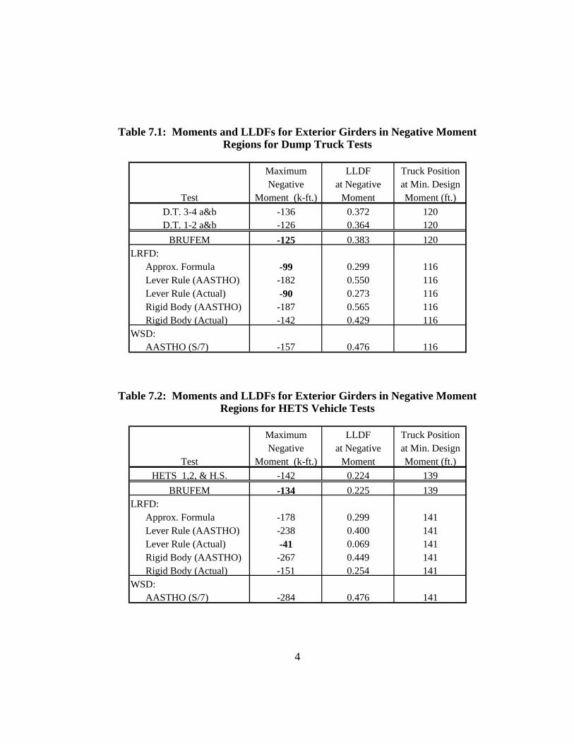
Table 7.1: Moments and LLDFs for Exterior Girders in Negative Moment Regions for Dump Truck Tests

Maximum LLDF Truck PositionNegative at Negative at Min. Design

Test Moment (k-ft.) Moment Moment (ft.)D.T. 3-4 a&b -136 0.372 120D.T. 1-2 a&b -126 0.364 120

BRUFEM -125 0.383 120LRFD: Approx. Formula -99 0.299 116 Lever Rule (AASTHO) -182 0.550 116 Lever Rule (Actual) -90 0.273 116 Rigid Body (AASTHO) -187 0.565 116 Rigid Body (Actual) -142 0.429 116WSD: AASTHO (S/7) -157 0.476 116

Table 7.2: Moments and LLDFs for Exterior Girders in Negative Moment Regions for HETS Vehicle Tests

Maximum LLDF Truck PositionNegative at Negative at Min. Design

Test Moment (k-ft.) Moment Moment (ft.)HETS 1,2, & H.S. -142 0.224 139

BRUFEM -134 0.225 139LRFD: Approx. Formula -178 0.299 141 Lever Rule (AASTHO) -238 0.400 141 Lever Rule (Actual) -41 0.069 141 Rigid Body (AASTHO) -267 0.449 141 Rigid Body (Actual) -151 0.254 141WSD: AASTHO (S/7) -284 0.476 141

4

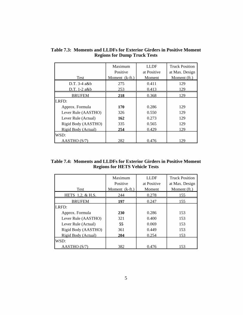
Table 7.3: Moments and LLDFs for Exterior Girders in Positive Moment Regions for Dump Truck Tests

Maximum LLDF Truck PositionPositive at Positive at Max. Design

Test Moment (k-ft.) Moment Moment (ft.)D.T. 3-4 a&b 275 0.411 129D.T. 1-2 a&b 253 0.413 129

BRUFEM 218 0.368 129LRFD: Approx. Formula 170 0.286 129 Lever Rule (AASTHO) 326 0.550 129 Lever Rule (Actual) 162 0.273 129 Rigid Body (AASTHO) 335 0.565 129 Rigid Body (Actual) 254 0.429 129WSD: AASTHO (S/7) 282 0.476 129

Table 7.4: Moments and LLDFs for Exterior Girders in Positive Moment Regions for HETS Vehicle Tests

Maximum LLDF Truck PositionPositive at Positive at Max. Design

Test Moment (k-ft.) Moment Moment (ft.)HETS 1,2, & H.S. 244 0.278 155

BRUFEM 197 0.247 155LRFD: Approx. Formula 230 0.286 153 Lever Rule (AASTHO) 321 0.400 153 Lever Rule (Actual) 55 0.069 153 Rigid Body (AASTHO) 361 0.449 153 Rigid Body (Actual) 204 0.254 153WSD: AASTHO (S/7) 382 0.476 153

5

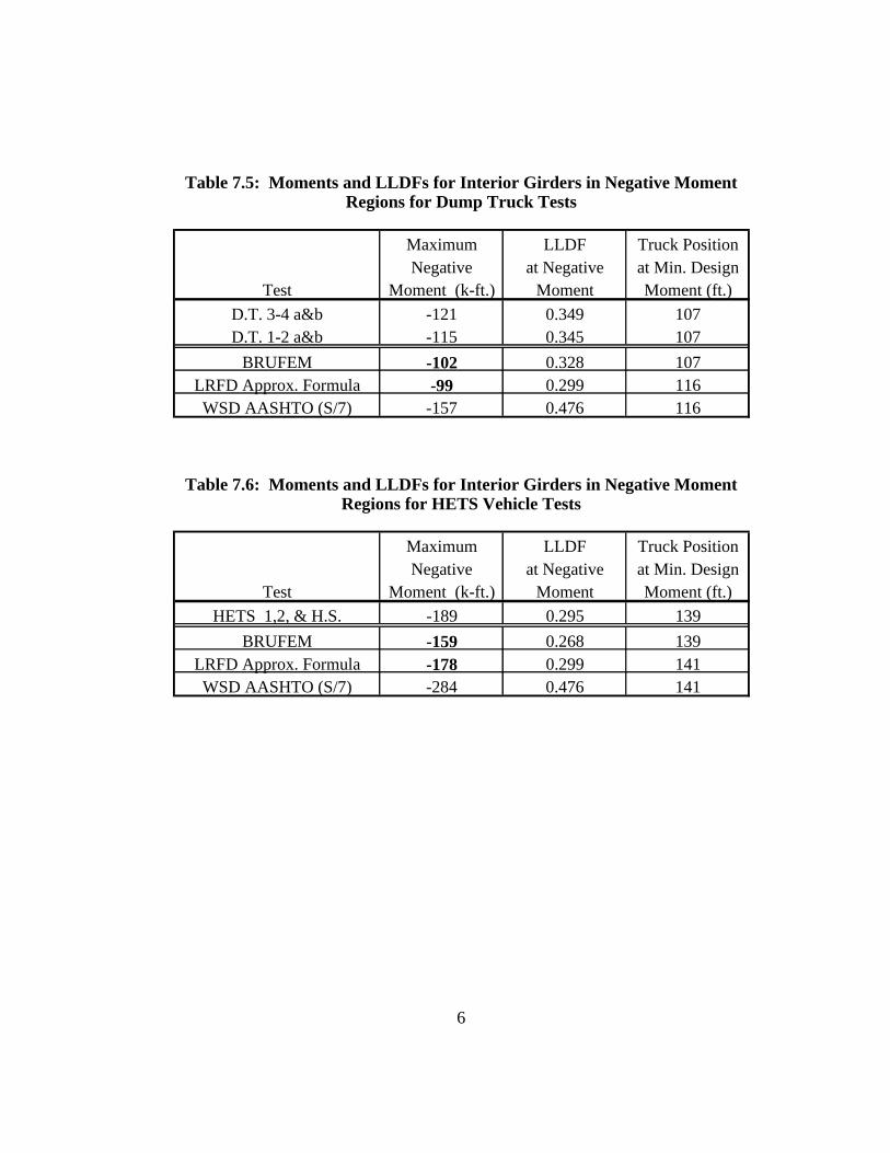
Table 7.5: Moments and LLDFs for Interior Girders in Negative Moment Regions for Dump Truck Tests

Maximum LLDF Truck PositionNegative at Negative at Min. Design

Test Moment (k-ft.) Moment Moment (ft.)D.T. 3-4 a&b -121 0.349 107D.T. 1-2 a&b -115 0.345 107

BRUFEM -102 0.328 107LRFD Approx. Formula -99 0.299 116WSD AASHTO (S/7) -157 0.476 116

Table 7.6: Moments and LLDFs for Interior Girders in Negative Moment Regions for HETS Vehicle Tests

Maximum LLDF Truck PositionNegative at Negative at Min. Design

Test Moment (k-ft.) Moment Moment (ft.)HETS 1,2, & H.S. -189 0.295 139

BRUFEM -159 0.268 139LRFD Approx. Formula -178 0.299 141WSD AASHTO (S/7) -284 0.476 141

6

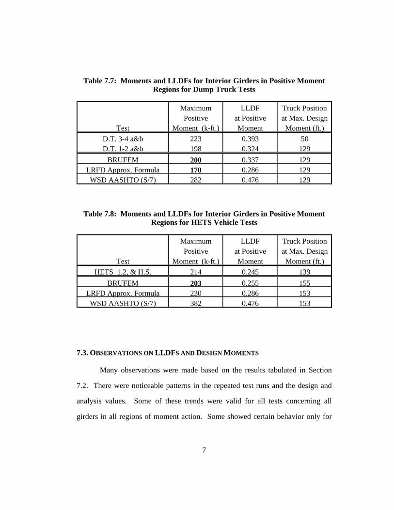
Table 7.7: Moments and LLDFs for Interior Girders in Positive Moment Regions for Dump Truck Tests

Maximum LLDF Truck PositionPositive at Positive at Max. Design

Test Moment (k-ft.) Moment Moment (ft.)D.T. 3-4 a&b 223 0.393 50D.T. 1-2 a&b 198 0.324 129

BRUFEM 200 0.337 129LRFD Approx. Formula 170 0.286 129WSD AASHTO (S/7) 282 0.476 129

Table 7.8: Moments and LLDFs for Interior Girders in Positive Moment Regions for HETS Vehicle Tests

Maximum LLDF Truck PositionPositive at Positive at Max. Design

Test Moment (k-ft.) Moment Moment (ft.)HETS 1,2, & H.S. 214 0.245 139

BRUFEM 203 0.255 155LRFD Approx. Formula 230 0.286 153WSD AASHTO (S/7) 382 0.476 153

7.3. OBSERVATIONS ON LLDFS AND DESIGN MOMENTS

Many observations were made based on the results tabulated in Section

7.2. There were noticeable patterns in the repeated test runs and the design and

analysis values. Some of these trends were valid for all tests concerning all

girders in all regions of moment action. Some showed certain behavior only for

7

certain combinations. This section will summarize trends among the test data,

BRUFEM output, and design values.

7.3.1. Trends in Measured Values

A few significant trends could be seen in the tables given in Section 7.2.

The most striking observation initially made was that the maximum positive

girder moments measured from the HETS vehicle were about the same as those

measured from the dump truck. For example, in the case of exterior girders in

negative moment regions (Tables 7.1 and 7.2) the governing moments for both

vehicles fell within the 120-140k-ft range for tests at low-speed. Only the

negative moments found in Tables 7.5 and 7.6 did not follow this trend. Other

patterns noticed for each vehicle are cited in this section.

7.3.1.1. Dump Truck Tests

The values of moment and lateral load distribution factors for all the dump

truck tests were close to each other in value. This indicated very repeatable data

for the low-speed tests. The values from all the low-speed dump truck tests could

be compared even though the truck was run in two different locations. Recall that

the D.T. 1-2 tests and D.T. 3-4 tests were symmetric about the bridge centerline.

Therefore, where girders 1 or 2 gave the maximum moments in the D.T. 1-2 tests,

girders 3and 4 gave maximum moments for the D.T. 3-4 tests.

The maximum range of governing moments before an average was made

was 36k-ft for interior girders and was 34k-ft. for the exterior girders. The range

was large due to the behavior of the bridge under two different lateral locations of

the vehicle. The maximum range was within 20% of the average moments

8

measured. The corresponding LLDF values for all the slow tests were also

similar to each other in value.

The high-speed dump truck test did not have the same lateral position as

the other 4 dump truck tests. This was reflected in the values for the D.T.H.S.

test. The LLDFs for the high-speed test were not as great since the vehicle was

traveling down the center of the bridge. The governing moments could have been

smaller for the high-speed test because the distribution of moment had a greater

effect than did the impact of the vehicle.

7.3.1.2. HETS Vehicle Tests

The HETS test exhibited the highest degree of repeatability and did show

evidence of dynamic effects. In general, the data from the HETS H.S. test

matched well with its low-speed counterparts since the lateral location of the

vehicle was the same in both tests. The maximum difference before averaging

between any governing moments for HETS tests was 13k-ft (approximately 6% of

the measured moments). Some evidence of dynamic effects was seen in all HETS

moments except for the exterior girder in positive moment regions. However, the

presentation of moments in each gauged section given in Section 4.3.2 shows

better evidence of dynamic effects.

7.3.2. Comparison of BRUFEM Values

In general, the BRUFEM LLDF values did a satisfactory job

approximating the LLDFs from the vehicle tests. BRUFEM LLDFs were greater

than 8 of 16 average test values. However, the BRUFEM moments

underestimated the actual moments from tests in 13 of the 16 cases. This

9

phenomenon may have been caused more by the conservative nature of Fully

Composite method to estimate the girder moments than an unconservative

BRUFEM analysis.

7.3.3. Comparison of Design Values

The design methods used to estimate moments each have their own

variables and degree of safety. The AASHTO Working Stress Design Code

contains the least variables, and generally ends up being the most conservative

way to distribute moment laterally. The newer AASTHO LRFD equations

contain the most variables of any used in this research and attempt to more

accurately model bridge behavior. This section cites the performance of all the

design estimates with respect to the measured values.

7.3.3.1. AASTHO Working Stress Design

It was expected that the values given by the Working Stress Design code

would be the most conservative. This was due in part to the location of the test

truck. The dump truck was not located in the position that would give the largest

moments on the exterior girder. The moment and LLDF values given by

AASTHO WSD were the most conservative of all the design values with the

exception of the lever rule for the AASTHO position of the dump truck. On

average, AASTHO WSD moments were conservative by a factor of 1.3 for all the

dump truck cases and by a factor of 1.7 for the HETS cases. It was notable that

the WSD value matched the values for the dump truck 3-4 tests in Table 7.3

within 7k-ft even though the dump truck was not as close to the curb as the

AASTHO position dictates.

10

7.3.3.2. AASTHO LRFD Lever Rule and Rigid Body Analysis

The exterior girder methods gave different results depending on whether

an AASTHO or actual position was considered. It is important to note that all of

the lever rule values for the actual position gave unconservative values. The rigid

body values for exterior girders using actual vehicle positions were

unconservative as well. All of the lever rule and rigid body values for the

AASTHO positions were conservative, which should have been expected since

the dump truck was not in the AASHTO position during the test. The lever rule

values of moment were conservative by a factor of 1.4 for the dump truck and 1.5

for the HETS. The rigid body analysis values were conservative by a factor of 1.4

for the dump truck and 1.7 for the HETS.

7.3.3.3. AASTHO Load and Resistance Factor Design

The LRFD equation gave unconservative values for moment in all cases

involving the dump truck and for half of those involving the HETS. When the

LRFD moment was unconservative, it was so by 24% on average. When

conservative, the reduced moments were about 86% of what the LRFD equation

predicted. The AASTHO LRFD LLDFs for the interior girders were closer to the

measured values than were the AASHTO estimates for the exterior girders. This

was due to the correction factor, e, in Equation 6.4. The correction factor was not

greater than 1.0 and did not result in larger design moments for the exterior

girders. Again, if a more accurate reduction method were used, it was believed

that the LRFD moment values would fit quite well with the test values. Recall,

11

that Section 4.3.1 stated that the Fully Composite reduction method was

conservative by about 7.5% in regions of extreme moment.

7.4. MOMENT RANGES

The lateral load distribution factors reduced and summarized in this

chapter were not only used to compare LLDF values and girder moments. The

data was also used to investigate moment ranges. Calculation of moment ranges

is done to estimate the potential for fatigue problems in a bridge. The results of

this investigation are provided in the tables at the end of this section.

The design moment ranges for a girder were calculated using the LLDFs

determined from the design codes and the maximum positive and negative static

moments in the bridge. The LLDFs from the design codes do not account for the

location of the vehicle relative to the section when a maximum effect occurs. In

some cases the location of the vehicle that gives the maximum moment range is

far from the section considered. Therefore, it would be appropriate to use a LLDF

that takes into consideration where the vehicle is longitudinally.

Section 5.1.2 shows the redistribution of moment among girders with

increased vehicle distance. The actual girder moments and LLDFs were known

for all of the seven representative vehicle locations for both the test data and the

BRUFEM analysis. Figure 7.1 shows a moment history from test D.T. 3-4a for an

exterior and interior girder. The two vehicle positions that cause the maximum

positive and negative moment in those girders for the Mid-span action show are

50’ and 120’ respectively. The moment range taken for each girder is the

12

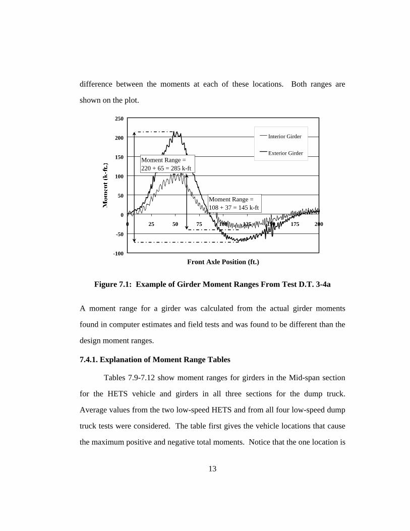
difference between the moments at each of these locations. Both ranges are

shown on the plot.

-100

-50

0

50

100

150

200

250

0 25 50 75 100 125 150 175 200

Front Axle Position (ft.)

Interior Girder

Exterior Girder

Moment Range = 108 + 37 = 145 k-ft

Moment Range = 220 + 65 = 285 k-ft

Figure 7.1: Example of Girder Moment Ranges From Test D.T. 3-4a

A moment range for a girder was calculated from the actual girder moments

found in computer estimates and field tests and was found to be different than the

design moment ranges.

7.4.1. Explanation of Moment Range Tables

Tables 7.9-7.12 show moment ranges for girders in the Mid-span section

for the HETS vehicle and girders in all three sections for the dump truck.

Average values from the two low-speed HETS and from all four low-speed dump

truck tests were considered. The table first gives the vehicle locations that cause

the maximum positive and negative total moments. Notice that the one location is

13

generally close to where the instrumentation was and the other is some distance

from it. The next column gives the unfactored moment range in the section.

These values are equal to the difference in maximum and minimum moments for

all the design methods and field tests.

The fourth and sixth columns give two LLDF values. The first is the

governing LLDF in the section for the first truck location; the second LLDF is the

value that governs at the second truck position. Except for BRUFEM estimates

and field tests, these values are the same for both vehicle locations. Treatment of

exterior and interior girders is handled in separate columns. The fifth and seventh

columns give the factored moment range for the governing girder. This value is

either the product of the design LLDFs and the line girder moments or an actual

moment range found in the BRUFEM output or vehicle test data.

For example, Table 7.9 shows values for the Mid-span section for dump

truck loading. Recall that the Mid-span section was located 35’ from the

beginning of the bridge. The second column shows that the maximum positive

effect in the cross-section occurred when the dump truck was at 50’ (close to the

section of interest). It also shows that the maximum negative effect in the cross-

section occurred when the dump truck was at 120’ (far from the section). The line

girder values taken from Figure 2.2 are 535k-ft at 50’ and -181k-ft at 120’. This

gives an total moment range of 535 - (-181) = 716k-ft. The BRUFEM and field

test ranges were obtained directly from computer output and reduced data at the

same vehicle locations.

14

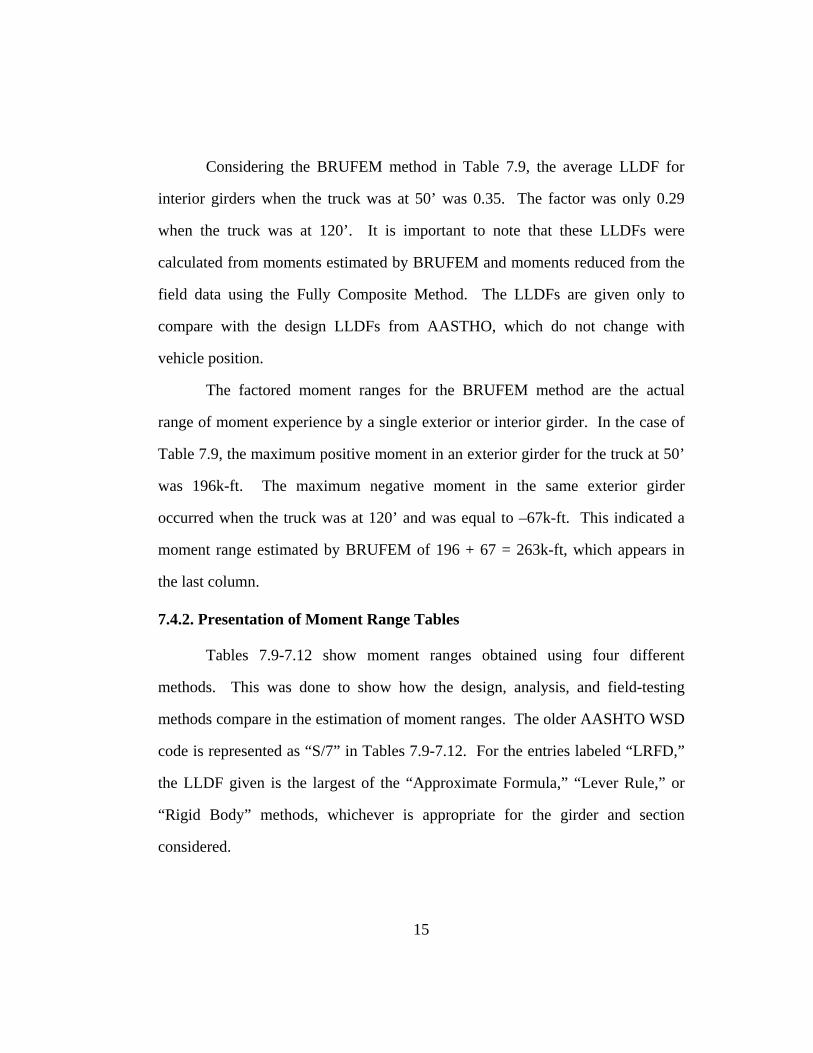
Considering the BRUFEM method in Table 7.9, the average LLDF for

interior girders when the truck was at 50’ was 0.35. The factor was only 0.29

when the truck was at 120’. It is important to note that these LLDFs were

calculated from moments estimated by BRUFEM and moments reduced from the

field data using the Fully Composite Method. The LLDFs are given only to

compare with the design LLDFs from AASTHO, which do not change with

vehicle position.

The factored moment ranges for the BRUFEM method are the actual

range of moment experience by a single exterior or interior girder. In the case of

Table 7.9, the maximum positive moment in an exterior girder for the truck at 50’

was 196k-ft. The maximum negative moment in the same exterior girder

occurred when the truck was at 120’ and was equal to –67k-ft. This indicated a

moment range estimated by BRUFEM of 196 + 67 = 263k-ft, which appears in

the last column.

7.4.2. Presentation of Moment Range Tables

Tables 7.9-7.12 show moment ranges obtained using four different

methods. This was done to show how the design, analysis, and field-testing

methods compare in the estimation of moment ranges. The older AASHTO WSD

code is represented as “S/7” in Tables 7.9-7.12. For the entries labeled “LRFD,”

the LLDF given is the largest of the “Approximate Formula,” “Lever Rule,” or

“Rigid Body” methods, whichever is appropriate for the girder and section

considered.

15

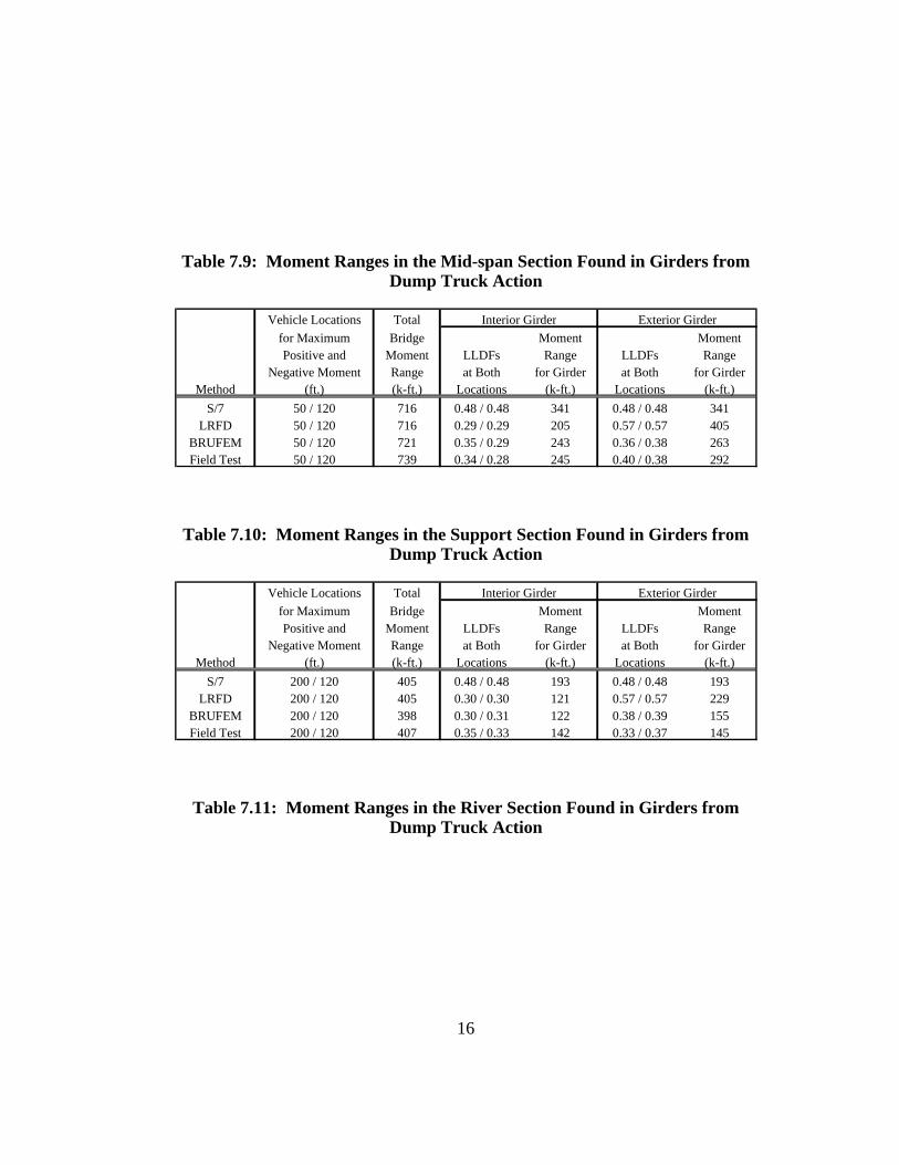
Table 7.9: Moment Ranges in the Mid-span Section Found in Girders from Dump Truck Action

Vehicle Locations Totalfor Maximum Bridge Moment MomentPositive and Moment LLDFs Range LLDFs Range

Negative Moment Range at Both for Girder at Both for GirderMethod (ft.) (k-ft.) Locations (k-ft.) Locations (k-ft.)

S/7 50 / 120 716 0.48 / 0.48 341 0.48 / 0.48 341LRFD 50 / 120 716 0.29 / 0.29 205 0.57 / 0.57 405

BRUFEM 50 / 120 721 0.35 / 0.29 243 0.36 / 0.38 263Field Test 50 / 120 739 0.34 / 0.28 245 0.40 / 0.38 292

Interior Girder Exterior Girder

Table 7.10: Moment Ranges in the Support Section Found in Girders from Dump Truck Action

Vehicle Locations Totalfor Maximum Bridge Moment MomentPositive and Moment LLDFs Range LLDFs Range

Negative Moment Range at Both for Girder at Both for GirderMethod (ft.) (k-ft.) Locations (k-ft.) Locations (k-ft.)

S/7 200 / 120 405 0.48 / 0.48 193 0.48 / 0.48 193LRFD 200 / 120 405 0.30 / 0.30 121 0.57 / 0.57 229

BRUFEM 200 / 120 398 0.30 / 0.31 122 0.38 / 0.39 155Field Test 200 / 120 407 0.35 / 0.33 142 0.33 / 0.37 145

Exterior GirderInterior Girder

Table 7.11: Moment Ranges in the River Section Found in Girders from Dump Truck Action

16

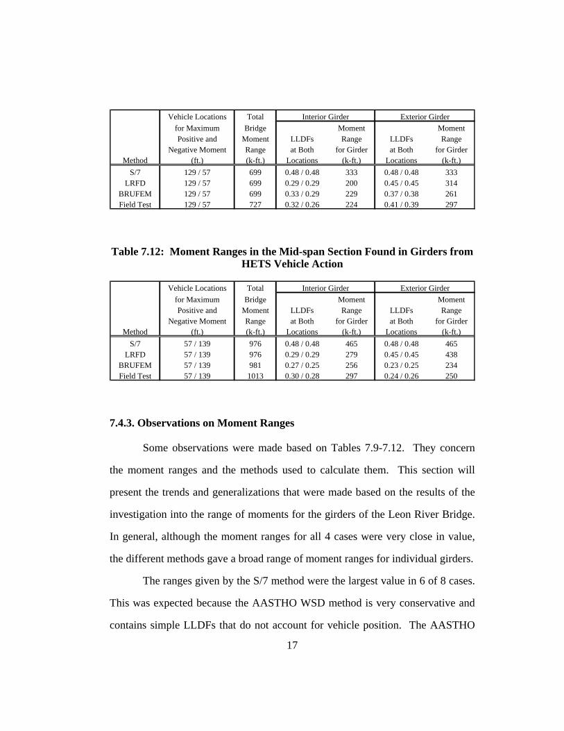
Vehicle Locations Totalfor Maximum Bridge Moment MomentPositive and Moment LLDFs Range LLDFs Range

Negative Moment Range at Both for Girder at Both for GirderMethod (ft.) (k-ft.) Locations (k-ft.) Locations (k-ft.)

S/7 129 / 57 699 0.48 / 0.48 333 0.48 / 0.48 333LRFD 129 / 57 699 0.29 / 0.29 200 0.45 / 0.45 314

BRUFEM 129 / 57 699 0.33 / 0.29 229 0.37 / 0.38 261Field Test 129 / 57 727 0.32 / 0.26 224 0.41 / 0.39 297

Exterior GirderInterior Girder

Table 7.12: Moment Ranges in the Mid-span Section Found in Girders from HETS Vehicle Action

Vehicle Locations Totalfor Maximum Bridge Moment MomentPositive and Moment LLDFs Range LLDFs Range

Negative Moment Range at Both for Girder at Both for GirderMethod (ft.) (k-ft.) Locations (k-ft.) Locations (k-ft.)

S/7 57 / 139 976 0.48 / 0.48 465 0.48 / 0.48 465LRFD 57 / 139 976 0.29 / 0.29 279 0.45 / 0.45 438

BRUFEM 57 / 139 981 0.27 / 0.25 256 0.23 / 0.25 234Field Test 57 / 139 1013 0.30 / 0.28 297 0.24 / 0.26 250

Interior Girder Exterior Girder

7.4.3. Observations on Moment Ranges

Some observations were made based on Tables 7.9-7.12. They concern

the moment ranges and the methods used to calculate them. This section will

present the trends and generalizations that were made based on the results of the

investigation into the range of moments for the girders of the Leon River Bridge.

In general, although the moment ranges for all 4 cases were very close in value,

the different methods gave a broad range of moment ranges for individual girders.

The ranges given by the S/7 method were the largest value in 6 of 8 cases.

This was expected because the AASTHO WSD method is very conservative and

contains simple LLDFs that do not account for vehicle position. The AASTHO

17

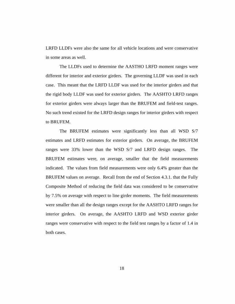
18

LRFD LLDFs were also the same for all vehicle locations and were conservative

in some areas as well.

The LLDFs used to determine the AASTHO LRFD moment ranges were

different for interior and exterior girders. The governing LLDF was used in each

case. This meant that the LRFD LLDF was used for the interior girders and that

the rigid body LLDF was used for exterior girders. The AASHTO LRFD ranges

for exterior girders were always larger than the BRUFEM and field-test ranges.

No such trend existed for the LRFD design ranges for interior girders with respect

to BRUFEM.

The BRUFEM estimates were significantly less than all WSD S/7

estimates and LRFD estimates for exterior girders. On average, the BRUFEM

ranges were 33% lower than the WSD S/7 and LRFD design ranges. The

BRUFEM estimates were, on average, smaller that the field measurements

indicated. The values from field measurements were only 6.4% greater than the

BRUFEM values on average. Recall from the end of Section 4.3.1. that the Fully

Composite Method of reducing the field data was considered to be conservative

by 7.5% on average with respect to line girder moments. The field measurements

were smaller than all the design ranges except for the AASHTO LRFD ranges for

interior girders. On average, the AASHTO LRFD and WSD exterior girder

ranges were conservative with respect to the field test ranges by a factor of 1.4 in

both cases.

Chapter 8: Conclusions and Recommendations

This research was successful in investigating the distribution of moment

laterally across the Leon River Bridge. It was also successful in investigating

design methods, dynamic effects, and moment ranges in girders. Key elements in

the completion of this research were testing the bridge in the field and modeling it

using SAP2000 and BRUFEM. In general, BRUFEM predicted moment and

behavior that were very close to measured values. The results of both field-

testing and BRUFEM modeling showed the lateral distribution of moment and

how that distribution was related to longitudinal vehicle position. The primary

use of the measured LLDFs was for comparison against LLDFs from various

design codes. The design values were conservative in most cases.

8.1. SUMMARY OF FINDINGS

There were a few observations made throughout the course of this

research that are significant enough to repeat here. The first point that should be

made is that the Leon River Bridge, although designed for noncomposite action,

did not behave noncompositely. The calculated N.A. locations and the results of

the Fully Composite Method of data reduction indicate some degree of composite

action. Other points made in this section cover the quality of the methods used in

this research, the repeatability and behavior found in the field tests, and trends

found in the LLDFs and moment ranges.

1

8.1.1. Moment Reduction Method

The Fully Composite Method used to reduce the data was chosen for two

reasons. First of all, the method recognized that the neutral axes of the girders

were such that some composite action was present. The method gave the best

estimate of moment values in regions of high strains. The other methods used

gave values that indicated that some moment was unaccounted for in the cross-

section. The method chosen was conservative in this respect and possibly gave

values that would make the LRFD and BRUFEM values appear unconservative.

The second reason why this method was chosen was its simplicity. Classical

equations and basic spreadsheets were all the tools required to reduce the acquired

strains into moments. A method of “partial composite action” is outlined in

Jauregui (1999) but was not used in this research.

8.1.2. Repeatability

The range in values obtained from all tests was remarkably small. This

indicated that the Leon River Bridge responded in a similar manner throughout all

the tests. This also signifies that that procedure used to instrument and test the

bridge was an acceptable method that gave accurate output. The data acquisition

system used for this research was well designed. It also shows that the person

using the manual switch, the driver of the vehicle, and the person running the data

acquisition system practiced good communication skills throughout all the tests.

8.1.3. Dynamic Effects

Conclusions on dynamic effects could only be made from the series of

HETS tests. Although additional vibration and oscillations were present in the

2

high-speed HETS test, the filtered results showed an increase in moment response

due to dynamic effects. Dynamic effects were most prevalent in the individual

girder values and present to a lesser effect in total moment at a section.

According to Tables 4.3 and 4.4, the average dynamic increase was 24% in

individual girders and 13% for total moment at a section. This data fit well with

the results of field tests used by AASHTO to determine impact factors. Section

3.6.2 of the AASHTO code indicates that the dynamic load allowance (IM) was

based on dynamic truck effects that cause increases of 25%.

8.1.4. Moment Distribution as a Function of Distance

Figures 5.4 through 5.9 in Chapter 5 depict the change in moment

distribution as a function of vehicle position. It was concluded that the girders

that take the majority of the load in primary moment action, still support the

majority of the load when the vehicle moved away onto an adjacent span.

However the range between moment percentages became smaller as vehicle

distance increased. BRUFEM performed well in estimating the LLDFs as a

function of distance.

This was significant because the stress range a girder experienced was

reduced because of this change in distribution. Section 7.4 showed how moment

ranges from the AASTHO LRFD and WSD methods were conservative with

respect to the BRUFEM estimates and field tests. The field tests were on average

only 6.4% greater than the BRUFEM estimates. This was notable especially

because the field tests were believed to be conservative by 7.5% in extreme

moment action.

3

8.1.5. Trends in Lateral Load Distribution Factors

Overall, the tests gave results with a high level of repeatability and

confidence. The BRUFEM and AASTHO LRFD LLDFs fit the test data

reasonably well since the reduction method was considered conservative in

nature. The degree to which the method was conservative could not be known for

certain, but was probably about 7-8%. Tables 7.1-7.8 showed that the AASHTO

LRFD moments were not as conservative as those calculated using the AASTHO

WSD (S/7) approach.

Most of cases using AASTHO methods for exterior girders using the

actual lateral location of the vehicle gave unconservative values. However all of

the values calculated using the AASTHO wheel locations (24” to curb) gave

conservative design values. As expected, conservative values were also given by

the older AASTHO WSD code in all cases.

8.2. PRACTICAL RESULTS

There were three types of practical results that were derived from this test.

These included recommendations about the testing procedure, the quality of

design methods, and insight into the Leon River Bridge behavior. The

conclusions and recommendations drawn here are based strictly on the researched

conducted.

8.2.1. Proposed Changes to the Bridge Instrumentation and Test Procedure

Adjustments to some of the strain gauging equipment have been made

since the time of the Leon River Test. Labeling of all wires that lead from the

gauge to the laptop was implemented to allow the repair of faulty channels in a

4

more organized manner. A shunt calibration system was also added to each

completion box in order to test each gauge with a predetermined strain. Based on

the results of this research, no additional hardware changes could be proposed that

would significantly improve the quality of data.

There was one change to the gauge layout that would result in better data

reduction. In the future, concrete gauges should be used on the bridge deck and

parapet portions of bridges of this type. These gauges would aid in determining

the degree of composite action of the bridge deck with the girders even though

non-composite action was expected. Strain data of this type would improve the

quality of data reduced by either a classical composite method such as the one

chosen in this research or the Moment-Couple Method presented, but not chosen.

In addition, data from gauges placed at the curbs would allow for a better model

of the contributing parapet portions.

A change to the lateral location of the dump truck would allow for more

meaning full comparisons of LLDFs. Many of the lever rule and rigid body

design moments given in Tables 7.1 and 7.3 appear conservative because the

AASHTO position used to calculate the design LLDF was different than the

actual position of the truck on the bridge. In future tests, the load vehicle should

be placed in the AASHTO position in order to make valid comparisons to the

AASTHO design methods for exterior girders.

8.2.2. Use of Design Methods for LLDF Calculation

The BRUFEM analysis package is a useful tool for bridge analysis. The

package contained appropriate modeling options that varied depending on the

5

type of bridge system. It was relatively easy to obtain LLDF values from the

BRUFEM output. The package was used mainly for this LLDF calculation and

contributed greatly to this research.

The results given by BRUFEM matched the field data very well. This

good correlation substantiated the modeling assumptions made in the BRUFEM

model. It was believed that the solution used for non-standard vehicle modeling

given in Section 2.3.2.2 and that to K-type diaphragm modeling given in Section

2.3.2.3 were satisfactory and had negligible impact on the results. In summary,

BRUFEM can be used with confidence as a preliminary design tool for moment

distribution in steel girder-slab bridges.

Considering the conservative nature of the Fully Composite method, the

AASTHO LRFD equations did a satisfactory job in estimating truck moments for

interior girders. The use of the AASHTO LRFD equations for exterior girders did

not produce good estimates. The geometry of the Leon River Bridge was such

that the LRFD correction factor for exterior girders had to be taken as 1.0. These

poor estimates of exterior girder LLDFs would lead to very conservative design

moments dictated by the AASHTO rigid body analysis LLDFs.

8.2.3. Insight Into Bridge Behavior

The current AASTHO lever rule, rigid body, and old AASTHO WSD

design methods for exterior girders were quite conservative in this case. The

Leon River Bridge was tested with a heavy dump truck in the appropriate lanes

and with an overload vehicle. Measured moments did not approach those

predicted by most equations for exterior girder design. This was due perhaps to

6

7

the participation of the deck slab in a degree of composite action that was not

anticipated in the design of the bridge.

Most overweight vehicles are longer and wider than typical vehicles. The

increased dimensions help reduce moment effects in two ways. The axles of the

61.7-foot long HETS vehicle were frequently in multiple spans, which reduces the

maximum positive moment a span will experience. Also the increased width

would warrant that the vehicle be driven down the center of the bridge. This

caused the load to be distributed almost equally among the four girders.

Therefore, most maximum individual girder moment values for the HETS were

similar to those obtained for the dump truck.

The equalizing of distribution factors with distance had a profound effect

on the design stress ranges for the girders. When the test vehicles progressed

away from a section, the moment was reversed, but also more spread out. This is

significant because an exterior girder may not take the as great a portion of the

maximum positive moment as it would the maximum negative moment at the

same location if the truck positions that cause the extremes differ by a large

distance. The AASHTO LRFD design methods currently do not have a method of

calculating stress ranges that takes this effect into consideration, therefore the

stress ranges used in design were very conservative in most cases. The actual

moment ranges were measured in this research and predicted by BRUFEM. The

BRUFEM estimates were easy to attain and were remarkably close to the moment

ranges taken directly from the field data. This effect should be studied further to

properly understand and predict the range of stresses seen by bridge girders.

Appendix A

BRUFEM Input Files

This appendix contains the input files used in the BRUFEM analysis

presented in this research. The HISTORY.PRE files are listed first. They contain

all the information for the BRUFUM analyses. Six HISTORY.PRE files are

listed, one for each type of analysis performed. The BAR.DAT file is presented

next and contains the geometry of the girders on the Leon River Bridge. The

VEH.DAT files used to model the non-standards vehicles are presented at the end

of this appendix.

A.1. HISTORY.PRE FILES FOR ALL BRUFEM ANALYSES

A.1.1. HISTORY.PRE File for the CGM Using the Dump Truck:

BEGIN_HISTORY_FILE -----<PROBLEM_TITLE>---------------------- DUMPTRUCK 3-4 CGMODEL (50,57,107,120,129,139,155) -----<BRIDGE_TYPE_IBTYPE>----------------- STL -----<TYPE_OF_UNITS>---------------------- 1 -----<VARIABLE/CONSTANT_SKEW>------------- 1 -----<PRIS_NONPRIS_IXSECT>---------------- 2 -----<STL_BASIC_MODEL_DATA>--------------- 4 6.6667 0 -----<ANALYSIS_TYPE_FULL/LIVE>------------ 1 -----<COMPOSITE_MODEL_TYPE>--------------- 2 -----<SLAB_THICK_STRENGTH>---------------- 6 4 -----<NUM_ELEM_BTWN_GIRD>-----------------

1

4 -----<NUM_SPANS>-------------------------- 3 -----<SPAN_LEN_&_NUM_Y_ELEMS>------------- 70 35 -----<SPAN_LEN_&_NUM_Y_ELEMS>------------- 90 45 -----<SPAN_LEN_&_NUM_Y_ELEMS>------------- 70 35 -----<STL_EFF_NEG_MOM>-------------------- 100 -----<STL_DIA_TYPE>----------------------- 2 -----<STL_DIA_CROSS_&_BTM_AREA>----------- 2.5 3.05 -----<STL_DIA_TOP_&_BTM_DIST>------------- 1.5 4.5 -----<ADDED_DIA_YESNO>-------------------- Y -----<ADDED_DIA_COUNT>-------------------- 11 -----<ADDED_DIA_DIST>--------------------- 20 40 55 85 100 115 130 145 175 190 210 -----<STL_HINGE_YESNO>-------------------- N -----<EXTRA_MEMBERS_YESNO>---------------- N -----<LEFT_EDGE_WIDTH_&_COUNT>------------ 2.8333 2 -----<RIGHT_EDGE_WIDTH_&_COUNT>----------- 2.8333 2 -----<TRAVEL_CLEARANCE_L_&_R>------------- 2.25 2.25 -----<VEH_LOAD_GROUP_01_YESNO>------------ Y -----<VEH_INPUT_FILE_INTER>--------------- F -----<VEH_POSITION_METHOD>---------------- 1 -----<VEH_POSITION_FWD/REV_X_Y>----------- F 164.5 607 -----<LANE_LOAD_DESC_YESNO>--------------- N -----<LANE_LOAD_COUNT>-------------------- 0 -----<MORE_LIVE_LOADS_01_YESNO>----------- Y -----<VEH_LOAD_GROUP_02_YESNO>------------ Y

2

-----<VEH_INPUT_FILE_INTER_SAME>---------- S -----<VEH_POSITION_METHOD>---------------- 1 -----<VEH_POSITION_FWD/REV_X_Y>----------- F 164.5 691 -----<LANE_LOAD_DESC_YESNO>--------------- N -----<LANE_LOAD_COUNT>-------------------- 0 -----<MORE_LIVE_LOADS_02_YESNO>----------- Y -----<VEH_LOAD_GROUP_03_YESNO>------------ Y -----<VEH_INPUT_FILE_INTER_SAME>---------- S -----<VEH_POSITION_METHOD>---------------- 1 -----<VEH_POSITION_FWD/REV_X_Y>----------- F 164.5 1291 -----<LANE_LOAD_DESC_YESNO>--------------- N -----<LANE_LOAD_COUNT>-------------------- 0 -----<MORE_LIVE_LOADS_03_YESNO>----------- Y -----<VEH_LOAD_GROUP_04_YESNO>------------ Y -----<VEH_INPUT_FILE_INTER_SAME>---------- S -----<VEH_POSITION_METHOD>---------------- 1 -----<VEH_POSITION_FWD/REV_X_Y>----------- F 164.5 1447 -----<LANE_LOAD_DESC_YESNO>--------------- N -----<LANE_LOAD_COUNT>-------------------- 0 -----<MORE_LIVE_LOADS_04_YESNO>----------- Y -----<VEH_LOAD_GROUP_05_YESNO>------------ Y -----<VEH_INPUT_FILE_INTER_SAME>---------- S -----<VEH_POSITION_METHOD>---------------- 1 -----<VEH_POSITION_FWD/REV_X_Y>----------- F 164.5 1555 -----<LANE_LOAD_DESC_YESNO>---------------

3

N -----<LANE_LOAD_COUNT>-------------------- 0 -----<MORE_LIVE_LOADS_05_YESNO>----------- Y -----<VEH_LOAD_GROUP_06_YESNO>------------ Y -----<VEH_INPUT_FILE_INTER_SAME>---------- S -----<VEH_POSITION_METHOD>---------------- 1 -----<VEH_POSITION_FWD/REV_X_Y>----------- F 164.5 1675 -----<LANE_LOAD_DESC_YESNO>--------------- N -----<LANE_LOAD_COUNT>-------------------- 0 -----<MORE_LIVE_LOADS_06_YESNO>----------- Y -----<VEH_LOAD_GROUP_07_YESNO>------------ Y -----<VEH_INPUT_FILE_INTER_SAME>---------- S -----<VEH_POSITION_METHOD>---------------- 1 -----<VEH_POSITION_FWD/REV_X_Y>----------- F 164.5 1867 -----<LANE_LOAD_DESC_YESNO>--------------- N -----<LANE_LOAD_COUNT>-------------------- 0 -----<MORE_LIVE_LOADS_07_YESNO>----------- N -----<VEH_OMIT_NONCRIT_CASES_YESNO>------- N -----<FEM_OUTPUT_QUANTITY>---------------- 2 -----<SELECTIVE_OUTPUT_FLAGS>------------- Y Y Y Y Y Y Y -----<GRAPHICS_PLOTTING_YESNO>------------ Y END_HISTORY_FILE

4

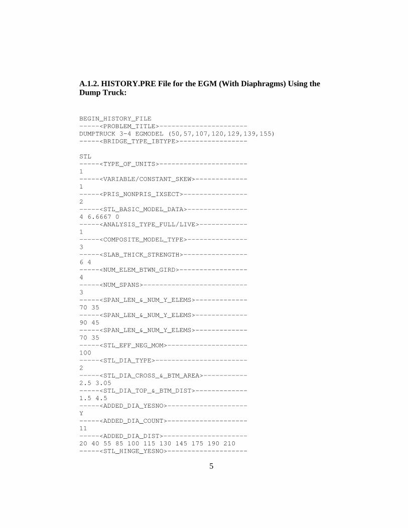
A.1.2. HISTORY.PRE File for the EGM (With Diaphragms) Using the Dump Truck:

BEGIN_HISTORY_FILE -----<PROBLEM_TITLE>---------------------- DUMPTRUCK 3-4 EGMODEL (50,57,107,120,129,139,155) -----<BRIDGE_TYPE_IBTYPE>----------------- STL -----<TYPE_OF_UNITS>---------------------- 1 -----<VARIABLE/CONSTANT_SKEW>------------- 1 -----<PRIS_NONPRIS_IXSECT>---------------- 2 -----<STL_BASIC_MODEL_DATA>--------------- 4 6.6667 0 -----<ANALYSIS_TYPE_FULL/LIVE>------------ 1 -----<COMPOSITE_MODEL_TYPE>--------------- 3 -----<SLAB_THICK_STRENGTH>---------------- 6 4 -----<NUM_ELEM_BTWN_GIRD>----------------- 4 -----<NUM_SPANS>-------------------------- 3 -----<SPAN_LEN_&_NUM_Y_ELEMS>------------- 70 35 -----<SPAN_LEN_&_NUM_Y_ELEMS>------------- 90 45 -----<SPAN_LEN_&_NUM_Y_ELEMS>------------- 70 35 -----<STL_EFF_NEG_MOM>-------------------- 100 -----<STL_DIA_TYPE>----------------------- 2 -----<STL_DIA_CROSS_&_BTM_AREA>----------- 2.5 3.05 -----<STL_DIA_TOP_&_BTM_DIST>------------- 1.5 4.5 -----<ADDED_DIA_YESNO>-------------------- Y -----<ADDED_DIA_COUNT>-------------------- 11 -----<ADDED_DIA_DIST>--------------------- 20 40 55 85 100 115 130 145 175 190 210 -----<STL_HINGE_YESNO>--------------------

5

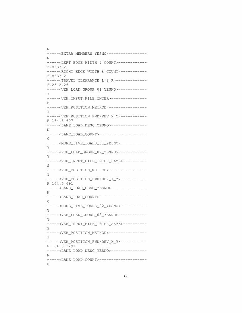
N -----<EXTRA_MEMBERS_YESNO>---------------- N -----<LEFT_EDGE_WIDTH_&_COUNT>------------ 2.8333 2 -----<RIGHT_EDGE_WIDTH_&_COUNT>----------- 2.8333 2 -----<TRAVEL_CLEARANCE_L_&_R>------------- 2.25 2.25 -----<VEH_LOAD_GROUP_01_YESNO>------------ Y -----<VEH_INPUT_FILE_INTER>--------------- F -----<VEH_POSITION_METHOD>---------------- 1 -----<VEH_POSITION_FWD/REV_X_Y>----------- F 164.5 607 -----<LANE_LOAD_DESC_YESNO>--------------- N -----<LANE_LOAD_COUNT>-------------------- 0 -----<MORE_LIVE_LOADS_01_YESNO>----------- Y -----<VEH_LOAD_GROUP_02_YESNO>------------ Y -----<VEH_INPUT_FILE_INTER_SAME>---------- S -----<VEH_POSITION_METHOD>---------------- 1 -----<VEH_POSITION_FWD/REV_X_Y>----------- F 164.5 691 -----<LANE_LOAD_DESC_YESNO>--------------- N -----<LANE_LOAD_COUNT>-------------------- 0 -----<MORE_LIVE_LOADS_02_YESNO>----------- Y -----<VEH_LOAD_GROUP_03_YESNO>------------ Y -----<VEH_INPUT_FILE_INTER_SAME>---------- S -----<VEH_POSITION_METHOD>---------------- 1 -----<VEH_POSITION_FWD/REV_X_Y>----------- F 164.5 1291 -----<LANE_LOAD_DESC_YESNO>--------------- N -----<LANE_LOAD_COUNT>-------------------- 0

6

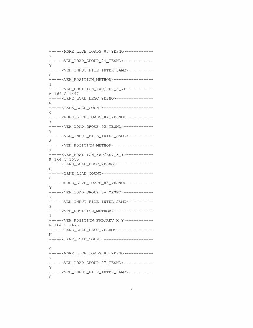
-----<MORE_LIVE_LOADS_03_YESNO>----------- Y -----<VEH_LOAD_GROUP_04_YESNO>------------ Y -----<VEH_INPUT_FILE_INTER_SAME>---------- S -----<VEH_POSITION_METHOD>---------------- 1 -----<VEH_POSITION_FWD/REV_X_Y>----------- F 164.5 1447 -----<LANE_LOAD_DESC_YESNO>--------------- N -----<LANE_LOAD_COUNT>-------------------- 0 -----<MORE_LIVE_LOADS_04_YESNO>----------- Y -----<VEH_LOAD_GROUP_05_YESNO>------------ Y -----<VEH_INPUT_FILE_INTER_SAME>---------- S -----<VEH_POSITION_METHOD>---------------- 1 -----<VEH_POSITION_FWD/REV_X_Y>----------- F 164.5 1555 -----<LANE_LOAD_DESC_YESNO>--------------- N -----<LANE_LOAD_COUNT>-------------------- 0 -----<MORE_LIVE_LOADS_05_YESNO>----------- Y -----<VEH_LOAD_GROUP_06_YESNO>------------ Y -----<VEH_INPUT_FILE_INTER_SAME>---------- S -----<VEH_POSITION_METHOD>---------------- 1 -----<VEH_POSITION_FWD/REV_X_Y>----------- F 164.5 1675 -----<LANE_LOAD_DESC_YESNO>--------------- N -----<LANE_LOAD_COUNT>-------------------- 0 -----<MORE_LIVE_LOADS_06_YESNO>----------- Y -----<VEH_LOAD_GROUP_07_YESNO>------------ Y -----<VEH_INPUT_FILE_INTER_SAME>---------- S

7

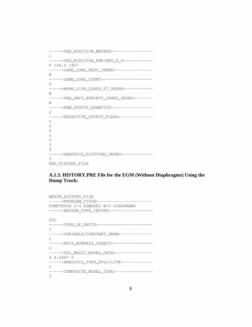
-----<VEH_POSITION_METHOD>---------------- 1 -----<VEH_POSITION_FWD/REV_X_Y>----------- F 164.5 1867 -----<LANE_LOAD_DESC_YESNO>--------------- N -----<LANE_LOAD_COUNT>-------------------- 0 -----<MORE_LIVE_LOADS_07_YESNO>----------- N -----<VEH_OMIT_NONCRIT_CASES_YESNO>------- N -----<FEM_OUTPUT_QUANTITY>---------------- 2 -----<SELECTIVE_OUTPUT_FLAGS>------------- Y Y Y Y Y Y Y -----<GRAPHICS_PLOTTING_YESNO>------------ Y END_HISTORY_FILE

A.1.3. HISTORY.PRE File for the EGM (Without Diaphragms) Using the Dump Truck:

BEGIN_HISTORY_FILE -----<PROBLEM_TITLE>---------------------- DUMPTRUCK 3-4 EGMODEL W/O DIAPHRAMS -----<BRIDGE_TYPE_IBTYPE>----------------- STL -----<TYPE_OF_UNITS>---------------------- 1 -----<VARIABLE/CONSTANT_SKEW>------------- 1 -----<PRIS_NONPRIS_IXSECT>---------------- 2 -----<STL_BASIC_MODEL_DATA>--------------- 4 6.6667 0 -----<ANALYSIS_TYPE_FULL/LIVE>------------ 1 -----<COMPOSITE_MODEL_TYPE>--------------- 3

8

-----<SLAB_THICK_STRENGTH>---------------- 6 4 -----<NUM_ELEM_BTWN_GIRD>----------------- 4 -----<NUM_SPANS>-------------------------- 3 -----<SPAN_LEN_&_NUM_Y_ELEMS>------------- 70 35 -----<SPAN_LEN_&_NUM_Y_ELEMS>------------- 90 45 -----<SPAN_LEN_&_NUM_Y_ELEMS>------------- 70 35 -----<STL_EFF_NEG_MOM>-------------------- 100 -----<STL_DIA_TYPE>----------------------- 2 -----<STL_DIA_CROSS_&_BTM_AREA>----------- 2.5 3.05 -----<STL_DIA_TOP_&_BTM_DIST>------------- 1.5 4.5 -----<ADDED_DIA_YESNO>-------------------- N -----<STL_HINGE_YESNO>-------------------- N -----<EXTRA_MEMBERS_YESNO>---------------- N -----<LEFT_EDGE_WIDTH_&_COUNT>------------ 2.8333 2 -----<RIGHT_EDGE_WIDTH_&_COUNT>----------- 2.8333 2 -----<TRAVEL_CLEARANCE_L_&_R>------------- 2.25 2.25 -----<VEH_LOAD_GROUP_01_YESNO>------------ Y -----<VEH_INPUT_FILE_INTER>--------------- F -----<VEH_POSITION_METHOD>---------------- 1 -----<VEH_POSITION_FWD/REV_X_Y>----------- F 164.5 607 -----<LANE_LOAD_DESC_YESNO>--------------- N -----<LANE_LOAD_COUNT>-------------------- 0 -----<MORE_LIVE_LOADS_01_YESNO>----------- Y -----<VEH_LOAD_GROUP_02_YESNO>------------ Y -----<VEH_INPUT_FILE_INTER_SAME>----------

9

S -----<VEH_POSITION_METHOD>---------------- 1 -----<VEH_POSITION_FWD/REV_X_Y>----------- F 164.5 691 -----<LANE_LOAD_DESC_YESNO>--------------- N -----<LANE_LOAD_COUNT>-------------------- 0 -----<MORE_LIVE_LOADS_02_YESNO>----------- Y -----<VEH_LOAD_GROUP_03_YESNO>------------ Y -----<VEH_INPUT_FILE_INTER_SAME>---------- S -----<VEH_POSITION_METHOD>---------------- 1 -----<VEH_POSITION_FWD/REV_X_Y>----------- F 164.5 1291 -----<LANE_LOAD_DESC_YESNO>--------------- N -----<LANE_LOAD_COUNT>-------------------- 0 -----<MORE_LIVE_LOADS_03_YESNO>----------- Y -----<VEH_LOAD_GROUP_04_YESNO>------------ Y -----<VEH_INPUT_FILE_INTER_SAME>---------- S -----<VEH_POSITION_METHOD>---------------- 1 -----<VEH_POSITION_FWD/REV_X_Y>----------- F 164.5 1447 -----<LANE_LOAD_DESC_YESNO>--------------- N -----<LANE_LOAD_COUNT>-------------------- 0 -----<MORE_LIVE_LOADS_04_YESNO>----------- Y -----<VEH_LOAD_GROUP_05_YESNO>------------ Y -----<VEH_INPUT_FILE_INTER_SAME>---------- S -----<VEH_POSITION_METHOD>---------------- 1 -----<VEH_POSITION_FWD/REV_X_Y>----------- F 164.5 1555 -----<LANE_LOAD_DESC_YESNO>--------------- N

10

-----<LANE_LOAD_COUNT>-------------------- 0 -----<MORE_LIVE_LOADS_05_YESNO>----------- Y -----<VEH_LOAD_GROUP_06_YESNO>------------ Y -----<VEH_INPUT_FILE_INTER_SAME>---------- S -----<VEH_POSITION_METHOD>---------------- 1 -----<VEH_POSITION_FWD/REV_X_Y>----------- F 164.5 1675 -----<LANE_LOAD_DESC_YESNO>--------------- N -----<LANE_LOAD_COUNT>-------------------- 0 -----<MORE_LIVE_LOADS_06_YESNO>----------- Y -----<VEH_LOAD_GROUP_07_YESNO>------------ Y -----<VEH_INPUT_FILE_INTER_SAME>---------- S -----<VEH_POSITION_METHOD>---------------- 1 -----<VEH_POSITION_FWD/REV_X_Y>----------- F 164.5 1867 -----<LANE_LOAD_DESC_YESNO>--------------- N -----<LANE_LOAD_COUNT>-------------------- 0 -----<MORE_LIVE_LOADS_07_YESNO>----------- N -----<VEH_OMIT_NONCRIT_CASES_YESNO>------- N -----<FEM_OUTPUT_QUANTITY>---------------- 2 -----<SELECTIVE_OUTPUT_FLAGS>------------- Y Y Y Y Y Y Y -----<GRAPHICS_PLOTTING_YESNO>------------ Y END_HISTORY_FILE

11

A.1.4. HISTORY.PRE File for the CGM Using the HETS Vehicle:

BEGIN_HISTORY_FILE -----<PROBLEM_TITLE>---------------------- HET CENTERED CGMODEL (50,57,107,120,129,139,155) -----<BRIDGE_TYPE_IBTYPE>----------------- STL -----<TYPE_OF_UNITS>---------------------- 1 -----<VARIABLE/CONSTANT_SKEW>------------- 1 -----<PRIS_NONPRIS_IXSECT>---------------- 2 -----<STL_BASIC_MODEL_DATA>--------------- 4 6.6667 0 -----<ANALYSIS_TYPE_FULL/LIVE>------------ 1 -----<COMPOSITE_MODEL_TYPE>--------------- 2 -----<SLAB_THICK_STRENGTH>---------------- 6 4 -----<NUM_ELEM_BTWN_GIRD>----------------- 4 -----<NUM_SPANS>-------------------------- 3 -----<SPAN_LEN_&_NUM_Y_ELEMS>------------- 70 35 -----<SPAN_LEN_&_NUM_Y_ELEMS>------------- 90 45 -----<SPAN_LEN_&_NUM_Y_ELEMS>------------- 70 35 -----<STL_EFF_NEG_MOM>-------------------- 100 -----<STL_DIA_TYPE>----------------------- 2 -----<STL_DIA_CROSS_&_BTM_AREA>----------- 2.5 3.05 -----<STL_DIA_TOP_&_BTM_DIST>------------- 1.5 4.5 -----<ADDED_DIA_YESNO>-------------------- Y -----<ADDED_DIA_COUNT>-------------------- 11 -----<ADDED_DIA_DIST>--------------------- 20 40 55 85 100 115 130 145 175 190 210 -----<STL_HINGE_YESNO>-------------------- N

12

-----<EXTRA_MEMBERS_YESNO>---------------- N -----<LEFT_EDGE_WIDTH_&_COUNT>------------ 2.8333 2 -----<RIGHT_EDGE_WIDTH_&_COUNT>----------- 2.8333 2 -----<TRAVEL_CLEARANCE_L_&_R>------------- 2.25 2.25 -----<VEH_LOAD_GROUP_01_YESNO>------------ Y -----<VEH_INPUT_FILE_INTER>--------------- F -----<VEH_POSITION_METHOD>---------------- 1 -----<VEH_POSITION_FWD/REV_X_Y>----------- F 120 607 -----<LANE_LOAD_DESC_YESNO>--------------- N -----<LANE_LOAD_COUNT>-------------------- 0 -----<MORE_LIVE_LOADS_01_YESNO>----------- Y -----<VEH_LOAD_GROUP_02_YESNO>------------ Y -----<VEH_INPUT_FILE_INTER_SAME>---------- S -----<VEH_POSITION_METHOD>---------------- 1 -----<VEH_POSITION_FWD/REV_X_Y>----------- F 120 691 -----<LANE_LOAD_DESC_YESNO>--------------- N -----<LANE_LOAD_COUNT>-------------------- 0 -----<MORE_LIVE_LOADS_02_YESNO>----------- Y -----<VEH_LOAD_GROUP_03_YESNO>------------ Y -----<VEH_INPUT_FILE_INTER_SAME>---------- S -----<VEH_POSITION_METHOD>---------------- 1 -----<VEH_POSITION_FWD/REV_X_Y>----------- F 120 1291 -----<LANE_LOAD_DESC_YESNO>--------------- N -----<LANE_LOAD_COUNT>-------------------- 0 -----<MORE_LIVE_LOADS_03_YESNO>-----------

13

Y -----<VEH_LOAD_GROUP_04_YESNO>------------ Y -----<VEH_INPUT_FILE_INTER_SAME>---------- S -----<VEH_POSITION_METHOD>---------------- 1 -----<VEH_POSITION_FWD/REV_X_Y>----------- F 120 1447 -----<LANE_LOAD_DESC_YESNO>--------------- N -----<LANE_LOAD_COUNT>-------------------- 0 -----<MORE_LIVE_LOADS_04_YESNO>----------- Y -----<VEH_LOAD_GROUP_05_YESNO>------------ Y -----<VEH_INPUT_FILE_INTER_SAME>---------- S -----<VEH_POSITION_METHOD>---------------- 1 -----<VEH_POSITION_FWD/REV_X_Y>----------- F 120 1555 -----<LANE_LOAD_DESC_YESNO>--------------- N -----<LANE_LOAD_COUNT>-------------------- 0 -----<MORE_LIVE_LOADS_05_YESNO>----------- Y -----<VEH_LOAD_GROUP_06_YESNO>------------ Y -----<VEH_INPUT_FILE_INTER_SAME>---------- S -----<VEH_POSITION_METHOD>---------------- 1 -----<VEH_POSITION_FWD/REV_X_Y>----------- F 120 1675 -----<LANE_LOAD_DESC_YESNO>--------------- N -----<LANE_LOAD_COUNT>-------------------- 0 -----<MORE_LIVE_LOADS_06_YESNO>----------- Y -----<VEH_LOAD_GROUP_07_YESNO>------------ Y -----<VEH_INPUT_FILE_INTER_SAME>---------- S -----<VEH_POSITION_METHOD>----------------

14

1 -----<VEH_POSITION_FWD/REV_X_Y>----------- F 120 1867 -----<LANE_LOAD_DESC_YESNO>--------------- N -----<LANE_LOAD_COUNT>-------------------- 0 -----<MORE_LIVE_LOADS_07_YESNO>----------- N -----<VEH_OMIT_NONCRIT_CASES_YESNO>------- N -----<FEM_OUTPUT_QUANTITY>---------------- 2 -----<SELECTIVE_OUTPUT_FLAGS>------------- Y Y Y Y Y Y Y -----<GRAPHICS_PLOTTING_YESNO>------------ Y END_HISTORY_FILE

A.1.5. HISTORY.PRE File for the EGM (With Diaphragms) Using the HETS Vehicle:

BEGIN_HISTORY_FILE -----<PROBLEM_TITLE>---------------------- HET CENTERED EGMODEL (50,57,107,120,129,139,155) -----<BRIDGE_TYPE_IBTYPE>----------------- STL -----<TYPE_OF_UNITS>---------------------- 1 -----<VARIABLE/CONSTANT_SKEW>------------- 1 -----<PRIS_NONPRIS_IXSECT>---------------- 2 -----<STL_BASIC_MODEL_DATA>--------------- 4 6.6667 0 -----<ANALYSIS_TYPE_FULL/LIVE>------------ 1 -----<COMPOSITE_MODEL_TYPE>--------------- 3 -----<SLAB_THICK_STRENGTH>----------------

15

6 4 -----<NUM_ELEM_BTWN_GIRD>----------------- 4 -----<NUM_SPANS>-------------------------- 3 -----<SPAN_LEN_&_NUM_Y_ELEMS>------------- 70 35 -----<SPAN_LEN_&_NUM_Y_ELEMS>------------- 90 45 -----<SPAN_LEN_&_NUM_Y_ELEMS>------------- 70 35 -----<STL_EFF_NEG_MOM>-------------------- 100 -----<STL_DIA_TYPE>----------------------- 2 -----<STL_DIA_CROSS_&_BTM_AREA>----------- 2.5 3.05 -----<STL_DIA_TOP_&_BTM_DIST>------------- 1.5 4.5 -----<ADDED_DIA_YESNO>-------------------- Y -----<ADDED_DIA_COUNT>-------------------- 11 -----<ADDED_DIA_DIST>--------------------- 20 40 55 85 100 115 130 145 175 190 210 -----<STL_HINGE_YESNO>-------------------- N -----<EXTRA_MEMBERS_YESNO>---------------- N -----<LEFT_EDGE_WIDTH_&_COUNT>------------ 2.8333 2 -----<RIGHT_EDGE_WIDTH_&_COUNT>----------- 2.8333 2 -----<TRAVEL_CLEARANCE_L_&_R>------------- 2.25 2.25 -----<VEH_LOAD_GROUP_01_YESNO>------------ Y -----<VEH_INPUT_FILE_INTER>--------------- F -----<VEH_POSITION_METHOD>---------------- 1 -----<VEH_POSITION_FWD/REV_X_Y>----------- F 120 607 -----<LANE_LOAD_DESC_YESNO>--------------- N -----<LANE_LOAD_COUNT>-------------------- 0 -----<MORE_LIVE_LOADS_01_YESNO>----------- Y

16

-----<VEH_LOAD_GROUP_02_YESNO>------------ Y -----<VEH_INPUT_FILE_INTER_SAME>---------- S -----<VEH_POSITION_METHOD>---------------- 1 -----<VEH_POSITION_FWD/REV_X_Y>----------- F 120 691 -----<LANE_LOAD_DESC_YESNO>--------------- N -----<LANE_LOAD_COUNT>-------------------- 0 -----<MORE_LIVE_LOADS_02_YESNO>----------- Y -----<VEH_LOAD_GROUP_03_YESNO>------------ Y -----<VEH_INPUT_FILE_INTER_SAME>---------- S -----<VEH_POSITION_METHOD>---------------- 1 -----<VEH_POSITION_FWD/REV_X_Y>----------- F 120 1291 -----<LANE_LOAD_DESC_YESNO>--------------- N -----<LANE_LOAD_COUNT>-------------------- 0 -----<MORE_LIVE_LOADS_03_YESNO>----------- Y -----<VEH_LOAD_GROUP_04_YESNO>------------ Y -----<VEH_INPUT_FILE_INTER_SAME>---------- S -----<VEH_POSITION_METHOD>---------------- 1 -----<VEH_POSITION_FWD/REV_X_Y>----------- F 120 1447 -----<LANE_LOAD_DESC_YESNO>--------------- N -----<LANE_LOAD_COUNT>-------------------- 0 -----<MORE_LIVE_LOADS_04_YESNO>----------- Y -----<VEH_LOAD_GROUP_05_YESNO>------------ Y -----<VEH_INPUT_FILE_INTER_SAME>---------- S -----<VEH_POSITION_METHOD>---------------- 1 -----<VEH_POSITION_FWD/REV_X_Y>-----------

17

F 120 1555 -----<LANE_LOAD_DESC_YESNO>--------------- N -----<LANE_LOAD_COUNT>-------------------- 0 -----<MORE_LIVE_LOADS_05_YESNO>----------- Y -----<VEH_LOAD_GROUP_06_YESNO>------------ Y -----<VEH_INPUT_FILE_INTER_SAME>---------- S -----<VEH_POSITION_METHOD>---------------- 1 -----<VEH_POSITION_FWD/REV_X_Y>----------- F 120 1675 -----<LANE_LOAD_DESC_YESNO>--------------- N -----<LANE_LOAD_COUNT>-------------------- 0 -----<MORE_LIVE_LOADS_06_YESNO>----------- Y -----<VEH_LOAD_GROUP_07_YESNO>------------ Y -----<VEH_INPUT_FILE_INTER_SAME>---------- S -----<VEH_POSITION_METHOD>---------------- 1 -----<VEH_POSITION_FWD/REV_X_Y>----------- F 120 1867 -----<LANE_LOAD_DESC_YESNO>--------------- N -----<LANE_LOAD_COUNT>-------------------- 0 -----<MORE_LIVE_LOADS_07_YESNO>----------- N -----<VEH_OMIT_NONCRIT_CASES_YESNO>------- N -----<FEM_OUTPUT_QUANTITY>---------------- 2 -----<SELECTIVE_OUTPUT_FLAGS>------------- Y Y Y Y Y Y Y -----<GRAPHICS_PLOTTING_YESNO>------------

18

Y END_HISTORY_FILE

A.1.6. HISTORY.PRE File for the EGM (Without Diaphragms) Using the HETS Vehicle:

BEGIN_HISTORY_FILE -----<PROBLEM_TITLE>---------------------- HET MODEL (EGM W/OUT DIAPHRAMS) -----<BRIDGE_TYPE_IBTYPE>----------------- STL -----<TYPE_OF_UNITS>---------------------- 1 -----<VARIABLE/CONSTANT_SKEW>------------- 1 -----<PRIS_NONPRIS_IXSECT>---------------- 2 -----<STL_BASIC_MODEL_DATA>--------------- 4 6.6667 0 -----<ANALYSIS_TYPE_FULL/LIVE>------------ 1 -----<COMPOSITE_MODEL_TYPE>--------------- 3 -----<SLAB_THICK_STRENGTH>---------------- 6 4 -----<NUM_ELEM_BTWN_GIRD>----------------- 4 -----<NUM_SPANS>-------------------------- 3 -----<SPAN_LEN_&_NUM_Y_ELEMS>------------- 70 35 -----<SPAN_LEN_&_NUM_Y_ELEMS>------------- 90 45 -----<SPAN_LEN_&_NUM_Y_ELEMS>------------- 70 35 -----<STL_EFF_NEG_MOM>-------------------- 100 -----<STL_DIA_TYPE>----------------------- 2 -----<STL_DIA_CROSS_&_BTM_AREA>----------- 2.5 3.05 -----<STL_DIA_TOP_&_BTM_DIST>------------- 1.5 4.5 -----<ADDED_DIA_YESNO>-------------------- N -----<STL_HINGE_YESNO>--------------------

19

N -----<EXTRA_MEMBERS_YESNO>---------------- N -----<LEFT_EDGE_WIDTH_&_COUNT>------------ 2.8333 2 -----<RIGHT_EDGE_WIDTH_&_COUNT>----------- 2.8333 2 -----<TRAVEL_CLEARANCE_L_&_R>------------- 2.25 2.25 -----<VEH_LOAD_GROUP_01_YESNO>------------ Y -----<VEH_INPUT_FILE_INTER>--------------- F -----<VEH_POSITION_METHOD>---------------- 1 -----<VEH_POSITION_FWD/REV_X_Y>----------- F 120 607 -----<LANE_LOAD_DESC_YESNO>--------------- N -----<LANE_LOAD_COUNT>-------------------- 0 -----<MORE_LIVE_LOADS_01_YESNO>----------- Y -----<VEH_LOAD_GROUP_02_YESNO>------------ Y -----<VEH_INPUT_FILE_INTER_SAME>---------- S -----<VEH_POSITION_METHOD>---------------- 1 -----<VEH_POSITION_FWD/REV_X_Y>----------- F 120 691 -----<LANE_LOAD_DESC_YESNO>--------------- N -----<LANE_LOAD_COUNT>-------------------- 0 -----<MORE_LIVE_LOADS_02_YESNO>----------- Y -----<VEH_LOAD_GROUP_03_YESNO>------------ Y -----<VEH_INPUT_FILE_INTER_SAME>---------- S -----<VEH_POSITION_METHOD>---------------- 1 -----<VEH_POSITION_FWD/REV_X_Y>----------- F 120 1291 -----<LANE_LOAD_DESC_YESNO>--------------- N -----<LANE_LOAD_COUNT>-------------------- 0

20

-----<MORE_LIVE_LOADS_03_YESNO>----------- Y -----<VEH_LOAD_GROUP_04_YESNO>------------ Y -----<VEH_INPUT_FILE_INTER_SAME>---------- S -----<VEH_POSITION_METHOD>---------------- 1 -----<VEH_POSITION_FWD/REV_X_Y>----------- F 120 1447 -----<LANE_LOAD_DESC_YESNO>--------------- N -----<LANE_LOAD_COUNT>-------------------- 0 -----<MORE_LIVE_LOADS_04_YESNO>----------- Y -----<VEH_LOAD_GROUP_05_YESNO>------------ Y -----<VEH_INPUT_FILE_INTER_SAME>---------- S -----<VEH_POSITION_METHOD>---------------- 1 -----<VEH_POSITION_FWD/REV_X_Y>----------- F 120 1555 -----<LANE_LOAD_DESC_YESNO>--------------- N -----<LANE_LOAD_COUNT>-------------------- 0 -----<MORE_LIVE_LOADS_05_YESNO>----------- Y -----<VEH_LOAD_GROUP_06_YESNO>------------ Y -----<VEH_INPUT_FILE_INTER_SAME>---------- S -----<VEH_POSITION_METHOD>---------------- 1 -----<VEH_POSITION_FWD/REV_X_Y>----------- F 120 1675 -----<LANE_LOAD_DESC_YESNO>--------------- N -----<LANE_LOAD_COUNT>-------------------- 0 -----<MORE_LIVE_LOADS_06_YESNO>----------- Y -----<VEH_LOAD_GROUP_07_YESNO>------------ Y -----<VEH_INPUT_FILE_INTER_SAME>---------- S

21

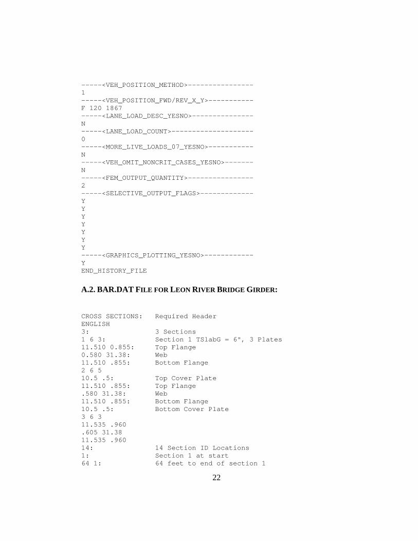
-----<VEH_POSITION_METHOD>---------------- 1 -----<VEH_POSITION_FWD/REV_X_Y>----------- F 120 1867 -----<LANE_LOAD_DESC_YESNO>--------------- N -----<LANE_LOAD_COUNT>-------------------- 0 -----<MORE_LIVE_LOADS_07_YESNO>----------- N -----<VEH_OMIT_NONCRIT_CASES_YESNO>------- N -----<FEM_OUTPUT_QUANTITY>---------------- 2 -----<SELECTIVE_OUTPUT_FLAGS>------------- Y Y Y Y Y Y Y -----<GRAPHICS_PLOTTING_YESNO>------------ Y END_HISTORY_FILE

A.2. BAR.DAT FILE FOR LEON RIVER BRIDGE GIRDER:

CROSS SECTIONS: Required Header ENGLISH 3: 3 Sections 1 6 3: Section 1 TSlabG = 6", 3 Plates 11.510 0.855: Top Flange 0.580 31.38: Web 11.510 .855: Bottom Flange 2 6 5 10.5 .5: Top Cover Plate 11.510 .855: Top Flange .580 31.38: Web 11.510 .855: Bottom Flange 10.5 .5: Bottom Cover Plate 3 6 3 11.535 .960 .605 31.38 11.535 .960 14: 14 Section ID Locations 1: Section 1 at start 64 1: 64 feet to end of section 1

22

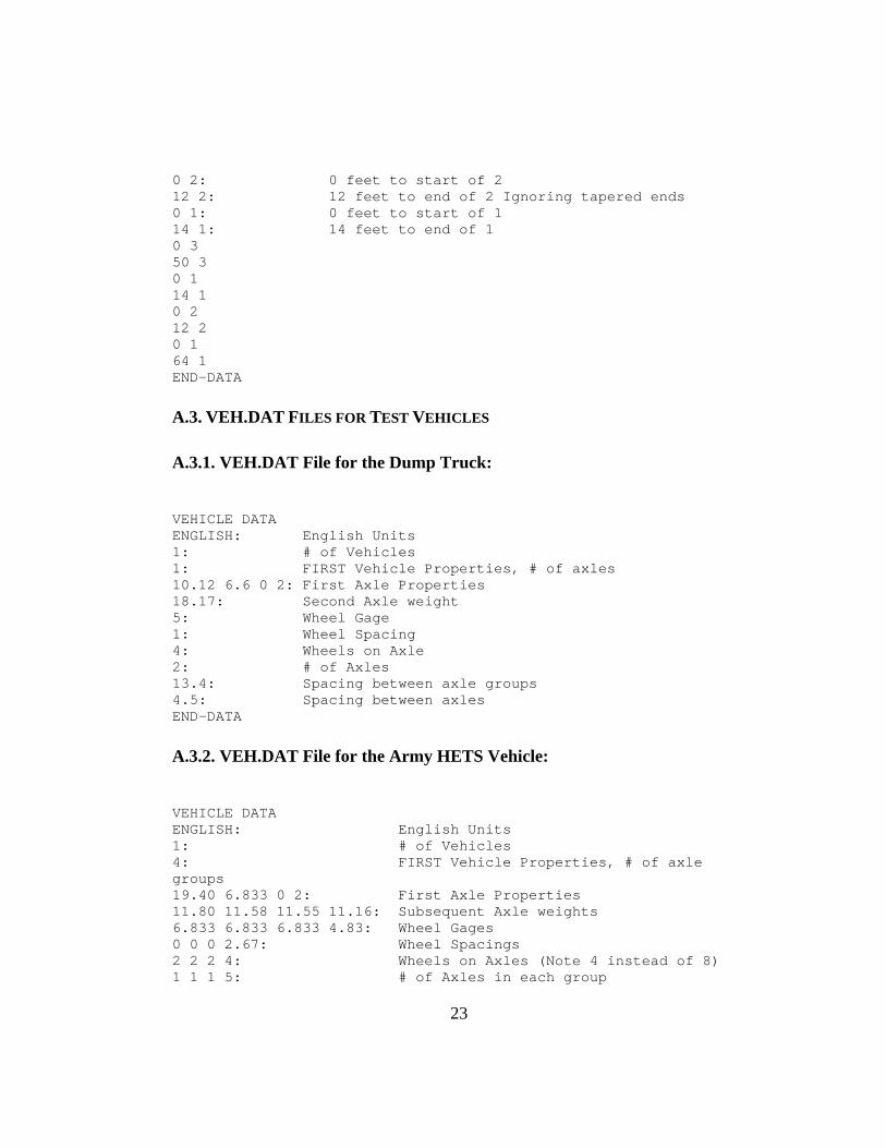
0 2: 0 feet to start of 2 12 2: 12 feet to end of 2 Ignoring tapered ends 0 1: 0 feet to start of 1 14 1: 14 feet to end of 1 0 3 50 3 0 1 14 1 0 2 12 2 0 1 64 1 END-DATA

A.3. VEH.DAT FILES FOR TEST VEHICLES

A.3.1. VEH.DAT File for the Dump Truck:

VEHICLE DATA ENGLISH: English Units 1: # of Vehicles 1: FIRST Vehicle Properties, # of axles 10.12 6.6 0 2: First Axle Properties 18.17: Second Axle weight 5: Wheel Gage 1: Wheel Spacing 4: Wheels on Axle 2: # of Axles 13.4: Spacing between axle groups 4.5: Spacing between axles END-DATA

A.3.2. VEH.DAT File for the Army HETS Vehicle:

VEHICLE DATA ENGLISH: English Units 1: # of Vehicles 4: FIRST Vehicle Properties, # of axle groups 19.40 6.833 0 2: First Axle Properties 11.80 11.58 11.55 11.16: Subsequent Axle weights 6.833 6.833 6.833 4.83: Wheel Gages 0 0 0 2.67: Wheel Spacings 2 2 2 4: Wheels on Axles (Note 4 instead of 8) 1 1 1 5: # of Axles in each group

23

12.917 5 5 15.104: Spacing between axle groups 0 0 0 5.938: Spacing between axles END-DATA

24

25

References

American Association of State Highway and Transportation Officals (AASHTO). (1998). LRFD Bridge Design Specifications, 2nd Edition, Washington D.C.

American Association of State Highway and Transportation Officals (AASHTO). (1992). Standard Specification for Highway Bridges, 15th Edition, Washington D.C.

Computers and Structures, Inc. (1997). “SAP2000 Analysis Reference–Volumes I and II.” Version 6.1.

Computers and Structures, Inc. (1997). “SAP2000 Getting Started–Basic Analysis Reference.” Version 6.1.

Hays Jr., C. O., Consolazio, G. R., Hoit, M.I., and Kakhandiki, A. (1994). “Bridge Rating of Girder-Slab Bridges Using Automated Finite Element Technology.” Structures Research Report No. 94-1, Department of Civil Engineering, University of Florida at Gainesville.

Jauregui, D. V. (1999). “Measurement-Based Evaluation of Non-Composite Steel Girder Bridges.” Doctorial Dissertation, University of Texas at Austin.

McIlrath, D. S. (1994). “Improving Bridge Rating and Truck Permitting Procedures Through Finite Element Analysis.” Master’s Thesis, University of Texas at Austin.