Copyright

by

Timothy Gordon Jones

2008

The Dissertation Committee for Timothy Gordon Jones

certifies that this is the approved version of the following dissertation:

Essays on Money, Inflation and Asset Prices

Committee:

Russell Cooper, Supervisor

Dean Corbae

Kim Ruhl

Jennifer Huang

M. Fatih Guvenen

Essays on Money, Inflation and Asset Prices

by

Timothy Gordon Jones, B.A.; M.S.

Dissertation

Presented to the Faculty of the Graduate School of

The University of Texas at Austin

in Partial Fulfillment

of the Requirements

for the Degree of

Doctor of Philosophy

The University of Texas at Austin

May 2008

Dedicated to Garrett, with love.

Acknowledgments

I would like to thank my advisor, Russell Cooper, whose guidance and support

have been essential both to this dissertation and to my professional development. I

am also grateful to Dean Corbae, Jennifer Huang, Kim Ruhl, and John Willis for

helpful advice and guidance. This work also benefited from useful comments from

the participants of numerous seminars at the department.

Additionally, Chai Chi, Patrick Cosgrove, Shayne McGuire, Kay Cuclis,

Phillip Auth, and KJ van Ackeren are a few of the excellent investment managers

at the Teacher Retirement System of Texas who assisted with their specific ideas

and general contributions to an open and productive exchange of ideas.

I am most grateful to Conan Crum, Jason DeBacker, Pablo D’Erasmo, Rick

Evans, and Anna Yurko for being supportive friends, excellent officemates, and

invaluable colleagues. This dissertation could not have been completed without

their advice and support.

Timothy Gordon Jones

The University of Texas at Austin

May 2008

v

Essays on Money, Inflation and Asset Prices

Publication No.

Timothy Gordon Jones, Ph.D.

The University of Texas at Austin, 2008

Supervisor: Russell Cooper

This dissertation explores different aspects of the interaction between money and

asset prices. The first chapter investigates how a firm’s financing affects its decision

to update prices: does linking interest rates to inflation alter the firm’s optimal price

updating strategy? Building on the state dependent pricing models of Willis (2000)

and the price indexing literature of Azariadis and Cooper (1985) and Freeman and

Tabellini (1998), this model investigates the financing and price updating decisions

of a representative firm facing state-dependent pricing and a cash-in-advance con-

straint. The model shows the circumstances under which a firm’s financing decision

affects its price updating decision, and how the likelihood of changing prices af-

fects the amount borrowed. It also illustrates how the use of nominal (as opposed

to inflation-linked) interest rates leads to a lower frequency of price updating and

vi

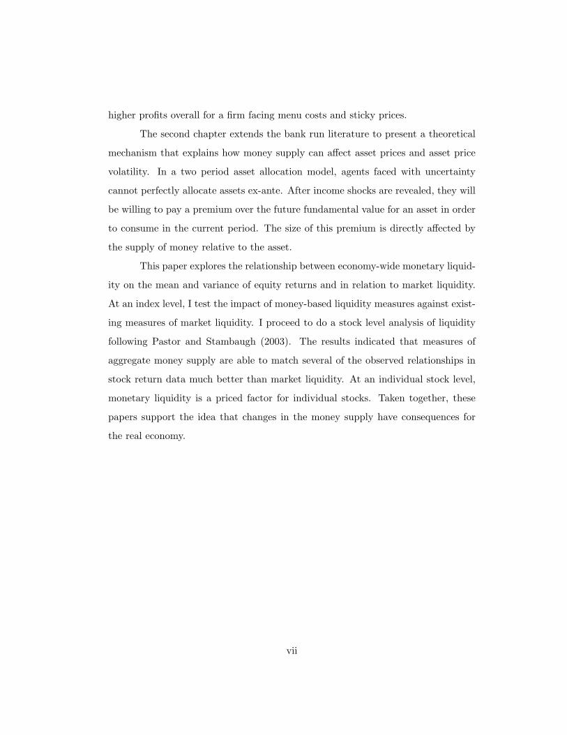
higher profits overall for a firm facing menu costs and sticky prices.

The second chapter extends the bank run literature to present a theoretical

mechanism that explains how money supply can affect asset prices and asset price

volatility. In a two period asset allocation model, agents faced with uncertainty

cannot perfectly allocate assets ex-ante. After income shocks are revealed, they will

be willing to pay a premium over the future fundamental value for an asset in order

to consume in the current period. The size of this premium is directly affected by

the supply of money relative to the asset.

This paper explores the relationship between economy-wide monetary liquid-

ity on the mean and variance of equity returns and in relation to market liquidity.

At an index level, I test the impact of money-based liquidity measures against exist-

ing measures of market liquidity. I proceed to do a stock level analysis of liquidity

following Pastor and Stambaugh (2003). The results indicated that measures of

aggregate money supply are able to match several of the observed relationships in

stock return data much better than market liquidity. At an individual stock level,

monetary liquidity is a priced factor for individual stocks. Taken together, these

papers support the idea that changes in the money supply have consequences for

the real economy.

vii

Contents

Acknowledgments v

Abstract vi

Chapter 1 Price and Interest Rate Indexing 1

1.1 Introduction . . . . . . . . . . . . . . . . . . . . . . . . . . . . . . . . 1

1.2 Model . . . . . . . . . . . . . . . . . . . . . . . . . . . . . . . . . . . 3

1.2.1 Sequence of Decisions . . . . . . . . . . . . . . . . . . . . . . 4

1.2.2 Uncertainty . . . . . . . . . . . . . . . . . . . . . . . . . . . . 5

1.2.3 Firm’s Problem . . . . . . . . . . . . . . . . . . . . . . . . . . 6

1.3 Solution . . . . . . . . . . . . . . . . . . . . . . . . . . . . . . . . . . 8

1.3.1 Solving the Firm’s Problem . . . . . . . . . . . . . . . . . . . 8

1.4 Results . . . . . . . . . . . . . . . . . . . . . . . . . . . . . . . . . . . 12

1.4.1 Price Updating Decision . . . . . . . . . . . . . . . . . . . . . 12

1.4.2 Financing Decision . . . . . . . . . . . . . . . . . . . . . . . . 23

1.4.3 Indexing Effects . . . . . . . . . . . . . . . . . . . . . . . . . 25

1.5 Conclusion . . . . . . . . . . . . . . . . . . . . . . . . . . . . . . . . 37

Chapter 2 Asset Prices and Money in a Two-Period Equilibrium 39

2.1 Introduction . . . . . . . . . . . . . . . . . . . . . . . . . . . . . . . . 39

2.2 Model . . . . . . . . . . . . . . . . . . . . . . . . . . . . . . . . . . . 41

viii

2.2.1 Timing and Uncertainty . . . . . . . . . . . . . . . . . . . . . 42

2.2.2 Household Problem . . . . . . . . . . . . . . . . . . . . . . . . 44

2.2.3 Market Clearing . . . . . . . . . . . . . . . . . . . . . . . . . 45

2.2.4 Equilibrium . . . . . . . . . . . . . . . . . . . . . . . . . . . . 46

2.3 Solving the Model . . . . . . . . . . . . . . . . . . . . . . . . . . . . 47

2.3.1 First period (t = 1) . . . . . . . . . . . . . . . . . . . . . . . . 47

2.3.2 Initial Period . . . . . . . . . . . . . . . . . . . . . . . . . . . 50

2.3.3 Household Problem . . . . . . . . . . . . . . . . . . . . . . . . 50

2.3.4 Initial Price, p0 . . . . . . . . . . . . . . . . . . . . . . . . . . 54

2.4 Results . . . . . . . . . . . . . . . . . . . . . . . . . . . . . . . . . . . 55

2.4.1 Impact of liquidity shocks on the mean and variance of p0 . . 55

2.4.2 Monetary Services Index . . . . . . . . . . . . . . . . . . . . . 58

2.5 Conclusion . . . . . . . . . . . . . . . . . . . . . . . . . . . . . . . . 64

Chapter 3 Monetary Liquidity and Asset Pricing 65

3.1 Introduction . . . . . . . . . . . . . . . . . . . . . . . . . . . . . . . . 65

3.2 Data . . . . . . . . . . . . . . . . . . . . . . . . . . . . . . . . . . . . 69

3.3 Testing Liquidity on Index Aggregates . . . . . . . . . . . . . . . . . 73

3.4 Testing Liquidity on a Cross-Section of Stocks . . . . . . . . . . . . . 76

3.5 Causality . . . . . . . . . . . . . . . . . . . . . . . . . . . . . . . . . 83

3.5.1 Impact of Monetary vs. Market Liquidity on Returns and

Volatility . . . . . . . . . . . . . . . . . . . . . . . . . . . . . 84

3.5.2 Causality between Market and Monetary Liquidity . . . . . . 88

3.6 Conclusion . . . . . . . . . . . . . . . . . . . . . . . . . . . . . . . . 90

Bibliography 91

Vita 94

ix

Chapter 1

Price and Interest Rate

Indexing

1.1 Introduction

In an environment where prices are costly to change, firms face a trade-off between

price inefficiency and adjustment costs. In not updating its price, a firm risks a

demand shock from inflation; its real price will be lower than optimal because of an

increase in the aggregate price level. The standard state-dependent pricing solution

is to update prices when the cost of adjusting prices is lower than the profit lost

from having a non-optimal price. Here we consider that a firm’s financing costs can

also be affected by the aggregate price level, and can feed back into the decision to

update prices. The amount borrowed impacts the price updating strategy through

the cash-in-advance constraint. In addition to borrowing, I compare two types of

interest rate regimes, one indexed to inflation (changes in the aggregate price level)

and the other not indexed. The type of interest rate regime alters the optimal

updating strategy of the firm; firms borrowing at non-indexed rates update prices

less frequently and have higher expected profits.

1

Before addressing the role of interest rate regimes, its necessary to estab-

lish how a financing decision can be relevant to a firm’s value in the first place.

Modiglianni and Miller (1958) proposition I, also called the irrelevance proposition,

maintains that under a set of basic market efficiency assumptions financing decisions

should not affect the core business of the firm. In order to consider price and inter-

est rate indexing, I am necessarily relaxing those assumptions in two ways. First,

I’m allowing sticky prices by imposing state-dependent costs on price adjustment.

Secondly, in order for firms to need financing in the first place, I introduce a cash-

in-advance constraint. The interaction between these two distortions results in the

relevance of financing structure to the firm’s price updating strategy and overall

value.

A cash-in-advance constraint is sufficient to contradict the irrelevance propo-

sition by itself; it can be considered a special case of incomplete asset markets. A

menu cost hinders price adjustment, which will affect firm value, though not nec-

essarily through the capital structure. The model shows how the amount a firm

borrows affects its price adjustment strategy by limiting the quantity it can pro-

duce. Moreover, the interaction of those frictions produces an environment where

the non-indexed interest rate regime generates higher expected profits for firms than

indexed ones. The model offers a mechanism to explain this outcome: indexing rates

deters borrowings and causes the cash-in-advance constraint to bind more severely.

Firms that do not index their borrowing have less to gain from price changes and

will therefore update prices less frequently, and borrow more.

Previous literature in this area has focused on the optimal risk sharing prop-

erties of nominal contracts (or the equivalent term, non-indexed prices). These

papers address models that share a common approach. Each of at least two agents

is a buyer of one good or service and a seller of another. Therefore, equilibria exist

when either everyone indexes their price or no one does. For an agent to pay an

2

indexed price but offer a non-indexed one would mean taking on a disproportionate

amount of risk. If ex-ante risk preferences were the same, this extra risk would not

be optimal. Blinder (1977) defines this relationship and the equilibrium between

worker’s wages and firm’s returns; Azariadis and Cooper (1985) for worker’s wages

and the price of goods. Freeman and Tabellini (1998) establishes the conditions

necessary for agents to choose a nominal, and therefore monetary, equilibrium.

This paper contributes to the literature by addressing the link between the

price of goods and interest rates. In what follows, I describe how a firm’s financing

mechanism can affect its overall value at all, and if so, under what conditions the firm

would be better off with non-indexed interest rates. I develop a partial equilibrium

model of the firm assuming some positive cost to adjusting its price. The firm

borrows before the menu cost and shocks to taste and inflation are revealed in order

to fund current production. The firm can change its price by paying the cost of

adjustment, or use last period’s price. I show that for positive costs of adjustment,

firms have higher expected profits for all initial price levels when borrowing at non-

indexed interest rates.

Section 2 details the environment of the model, the sequence of decisions, and

the firm’s problem. Section 3 solves the firm’s problem and defines equilibrium.

Section 4 shows how the financing constraint and non-indexed interest rates increase

price stickiness for a given menu cost, and goes on to prove the primary result, that

firms prefer non-indexed rates. A conclusion follows in Section 5.

1.2 Model

The model environment is one of two-period partial equilibrium, designed to high-

light the pricing behavior of a firm. The firm enters the first period with an initial

price and a unique production technology, converting labor into output. The de-

3

mand for its product is know to the firm and can purchase labor competitively. 1

Due to a cash-in-advance constraint, firms must borrow money in the first period

to produce in the second. If a firm opts to change its price, it has to pay a cost

of adjustment drawn in the second period. When the firm makes its financing

decision, it does so under uncertainty about demand, its real price, and the cost of

adjustment. Consider the choices a firm faces in the event of a high realization of

demand (from inflation or a taste shock). If the firm has borrowed more money

than it expected to use, it has additional capacity to hire workers and meet the high

demand rather than paying the menu cost and raising its price. This increased flex-

ibility comes at the price of higher borrowing costs. If the firm borrowed only what

it expected to need, the same high demand scenario makes it more likely that the

firm will pay the menu cost and raise its price rather than sell its limited quantity at

the initial price, which after the demand shock is much lower than the optimal reset

price. This uncertainty about demand connects the financing decision to the price

updating decision. The firm must decide on the amount to borrow, and thereby

commit to both an upper limit on how much it can produce and lower limit on its

costs. Those limits will affect its decision to update its price in the next period.

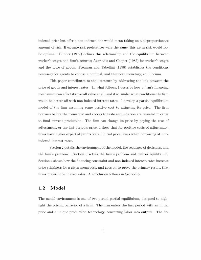
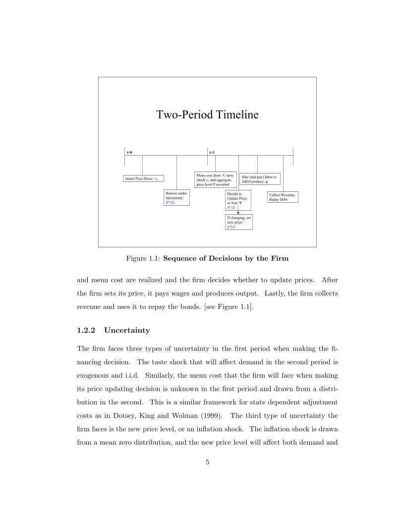
1.2.1 Sequence of Decisions

The first period is the financing period, when the firm must decide how much money

to borrow for use in the second period. In the second period, capital markets are

closed, and the firm must use what it has borrowed to hire workers and produce

goods. The interest rate, indexation regime, wages, and productivity are exogenous

and held constant. In the first period, before the shocks and menu cost are revealed,

the firm borrows by issuing one period bonds to finance current second period pro-

duction . After the first period’s borrowing is complete, the taste shock, price level,1The particular form of demand can be derived as an outcome of optimized CES preferences,

which is standard in the price adjustment literature.

4

Two-Period Timeline

Initial Price Draw: p-1

Collect Revenue, Repay Debt

Borrow under uncertainty: B*(S)

If changing, set new price: p*(S)

Hire (and pay) labor to fulfill produce: qs

t=0 t=1

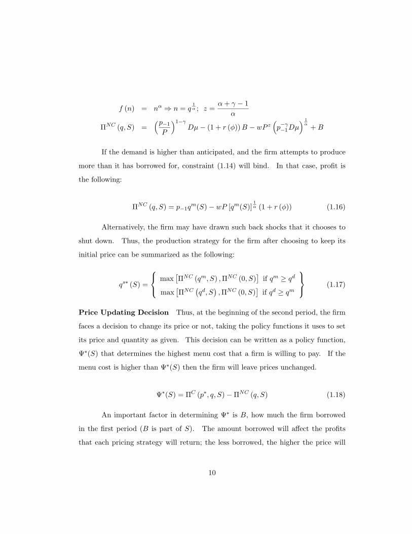
Menu cost draw Ψ, taste shock µ, and aggregate price level P revealed

Decide to Update Price or Not: ΨΨ’(S)

Figure 1.1: Sequence of Decisions by the Firm

and menu cost are realized and the firm decides whether to update prices. After

the firm sets its price, it pays wages and produces output. Lastly, the firm collects

revenue and uses it to repay the bonds. [see Figure 1.1].

1.2.2 Uncertainty

The firm faces three types of uncertainty in the first period when making the fi-

nancing decision. The taste shock that will affect demand in the second period is

exogenous and i.i.d. Similarly, the menu cost that the firm will face when making

its price updating decision is unknown in the first period and drawn from a distri-

bution in the second. This is a similar framework for state dependent adjustment

costs as in Dotsey, King and Wolman (1999). The third type of uncertainty the

firm faces is the new price level, or an inflation shock. The inflation shock is drawn

from a mean zero distribution, and the new price level will affect both demand and

5

the firm’s costs (see Equations 1.1 and 1.2).

logP = logP−1 + ε (1.1)

ε ∼ N (0, σ) (1.2)

1.2.3 Firm’s Problem

In the first period, the firm has an initial price (p−1) and knows the initial price

level (P−1). These two values define the ex-ante state, from which the firm takes

expectations about next period’s demand and costs. The firm then borrows in this

period in order to finance production. In the next period, the aggregate shock is

revealed and the firm decides if it should change its price or not.

Firm’s Optimization Problem

In the first period, the firm chooses an amount to borrow. In doing so, it must

take into account the realization of the shocks and its own strategy for updating the

price Equation (1.3) summarizes the first period problem. S−1 is a vector of state

variables known at the time of the financing decision, including the first period price

and aggregate price level. S includes the realizations of the random variables and

the choice of B.

Π (S−1) = maxBE[{

ΠC (p, q, S) ,ΠNC (q, S)}]

(1.3)

S−1 ={P−1, p−1, r

F , φ, λ}

(1.4)

S = {S−1, P,Ψ, µ,B} (1.5)

The two functions that are considered in the first period, ΠC (p, q, S) and

6

ΠNC (q, S), are the profit functions for the firm in the second period, after the

decision to change its price has been made. If the firm decides to change its

price, the second period firm’s problem is equation (1.6). The firm chooses a price

to maximize profits as well as the quantity to produce, subject to the borrowing

constraint and demand equation (1.8). If the firm chooses not to update its price

it simply chooses a quantity. This is meant to allow the firm the option to exit or

partially fulfill demand, not as a tool for optimization.

ΠC(p, q, S) = max{p,q}

pqs (p)− (1 + r (φ))B −

(wn

(P

P−1

)λ

−B

)−Ψ (1.6)

ΠNC(q, S) = max{q}

p−1qs (S)− (1 + r (φ))B −

(wn

(P

P−1

)λ

−B

)(1.7)

s.t. qs (S) ≤ min{qm (S) , qd (S)

}(1.8)

where qm =

[B

w

(P−1

P

)λ]α

; qdi (pi, P ) =

(pi

P

)−γ (D)P

µ; (1.9)

Demand for good i is CES (1.9), where D is a scaling parameter, µ is the

taste shock, γ is the elasticity parameter, P is the aggregate price level, and pi is

the price of a specific good.

The production technology converts labor to output:

qs = f (n) = nα

The structure of the interest rates facing the firm can depend on the price

level, as see above in r.

r =(1 + rF

) [Pt+1

Pt

]φ

(1.10)

The parameters {φ, λ} (1.6,1.7,1.10) define the indexation in the firm’s factor

contracts. φ determines the extent to which the interest rate changes with inflation,

7

while λ controls the extent to which the wage changes with inflation. if λ is zero,

the nominal wage does not change with the price level. If φ and λ are both 1, the

interest rate and the wage are effectively real costs. Ψ is the menu cost (the cost of

updating prices). Equation (1.8) highlights the effect the borrowing constraint has

on the quantity choice. The less a firm has borrowed in the first period, the lower

the maximum quantity it can produce, and the more likely qm will bind.

1.3 Solution

1.3.1 Solving the Firm’s Problem

The firm maximizes (1.3) subject to the cash-in-advance constraint (1.8). The

firm’s problem is solved backwards through the two periods. Solving the second

period first, the firm takes the realized values of µ, Ψ and P as given, and maximizes

profits conditional on changing the price or keeping last period’s price. With the

second period policy function established, the firm solves the first period problem

of how much to borrow, taking expectations over the realizations of the states and

second period policy functions as given.

Second Period

Firms enter the second period with an amount borrowed and a previous price, both

from last period. Current aggregate price level, P , the taste shock, µ, and the menu

cost Ψ, are revealed at that point. Working backwards, the firm’s last decision is to

choose a price to maximize profits, assuming it chooses to pay the adjustment cost.

Choice of Price when Updating When the firm decides to pay the menu cost,

it chooses a price p, (and implicitly, a quantity) to maximize profits subject to the

limits of the cash-in-advance constraint. Substituting demand (1.9) into (1.6) and

adding a Lagrangian multiplier (δ) on the cash in advance constraint reformulates

8

the firm’s problem as an unconstrained maximization:

ΠC (p, q, S) = maxp

( pP

)1−γDµ−Br (φ)− wP z

(p−γDµ

) 1α −Ψ (1.11)

−δ[qd (p)− qm (S)

]where z = λ+

γ − 1α

and Ψ is known

Solving the first order condition yields a policy rule for price setting, condi-

tional on updating the price. The optimal price, p∗, solves:

if δ = 0 : p∗ (S) =γ

α (γ − 1)w

(P

P−1

)(z−γ+1)

(Dµ)1−α

α (1.12)

if δ ≥ 0 : p∗ (S) = (Dµ)1γ

(B [P−1]

λ

w

)−αγ

Pλαγ

+1− 1γ (1.13)

Choice of Quantity when Keeping Initial Price If the firm opts to keep its

price from last period, then demand is determined by the outcome of the shocks

alone. The firm does not have to fulfill demand however; its finance constraint

could bind, or it might not be able to produce at a profit.

ΠNC (q, S) = maxqs

p−1qs (S)− (1 + r (φ))B − wPn+B

s.t.

qs (S) ≤ qm (S) (1.14)

qs (S) ≤ qd (S) (1.15)

First we consider what happens when the firm produces up to the level

demanded, i.e., when constraint (1.15) binds:

9

f (n) = nα ⇒ n = q1α ; z =

α+ γ − 1α

ΠNC (q, S) =(p−1

P

)1−γDµ− (1 + r (φ))B − wP z

(p−γ−1Dµ

) 1α +B

If the demand is higher than anticipated, and the firm attempts to produce

more than it has borrowed for, constraint (1.14) will bind. In that case, profit is

the following:

ΠNC (q, S) = p−1qm(S)− wP [qm(S)]

1α (1 + r (φ)) (1.16)

Alternatively, the firm may have drawn such back shocks that it chooses to

shut down. Thus, the production strategy for the firm after choosing to keep its

initial price can be summarized as the following:

qs∗ (S) =

max[ΠNC (qm, S) ,ΠNC (0, S)

]if qm ≥ qd

max[ΠNC

(qd, S

),ΠNC (0, S)

]if qd ≥ qm

(1.17)

Price Updating Decision Thus, at the beginning of the second period, the firm

faces a decision to change its price or not, taking the policy functions it uses to set

its price and quantity as given. This decision can be written as a policy function,

Ψ∗(S) that determines the highest menu cost that a firm is willing to pay. If the

menu cost is higher than Ψ∗(S) then the firm will leave prices unchanged.

Ψ∗(S) = ΠC (p∗, q, S)−ΠNC (q, S) (1.18)

An important factor in determining Ψ∗ is B, how much the firm borrowed

in the first period (B is part of S). The amount borrowed will affect the profits

that each pricing strategy will return; the less borrowed, the higher the price will

10

need to be take advantage of the reduced capacity. When the initial price is close

to or less than the optimal price (the price that would be chosen if the menu cost

were paid), under-borrowing raises the value of price adjustment, and increases the

threshold menu cost the firm is willing to pay. When the initial price is above the

optimal price, under-borrowing reduces the value of price adjustment. In that case,

constraining capacity offsets the inefficiency created by an initial price that was too

high relative to an unconstrained optimal price.

First Period

In the previous section, the firm solves its pricing problem conditional on an amount

previously borrowed. In the first period, the firm chooses an amount to borrow

based on the following policy rules for updating and setting its price:

B∗ (S−1) = max{B}

∫S

max{ΠC (p, q, S) ,ΠNC (q, S)

}dS (1.19)

This maximization is somewhat tricky, due to the choice of updating or not.

For each state, the firm must evaluate whether it will change prices or not, i.e., solve

for Ψ∗(S). Equation (1.19) can be rewritten as a strategy if we take Ψ∗(S) as given:

B∗ (S−1) = max{B}

∫S

ΠC (p, q, S) if Ψ ≤ Ψ∗(S)

ΠNC (q, S) if Ψ > Ψ∗(S)

dS (1.20)

Once it knows which profit function will be optimal in each state, it can choose

an amount to borrow that maximizes the expected profit. The problem with this

approach is that Ψ∗(S) itself is dependent upon B. Thus, the problem must be

solved numerically.

11

1.4 Results

The model produces two critical results. First, that the financing amount, B, affects

the price adjustment strategy of the firm. Conversely, the firm takes that strategy

into account when deciding on the amount to borrow. This mechanism is important

to identify as it underpins the second result, that the indexing regime (the value of

φ in the model) also affects the firm’s price adjustment strategy. Related to the

indexing result is the finding that the firm’s expected profits are higher at every

initial price under the non-indexing interest rate regime. In this section, I describe

each result in detail and explain the mechanism driving it.

1.4.1 Price Updating Decision

In order to show how the financing decision affects firm value, I show how the financ-

ing decision B∗ (S−1) affects the price updating decision. Ψ∗ (S) is the reservation

menu cost that determines whether the firm will update prices. If their realized

menu cost is above Ψ∗ (S) , they will not change prices. Ψ∗ (S) depends on the

difference between the profits under a new price and the old price (1.18).

Impact of Amount Borrowed on Price Updating Decision

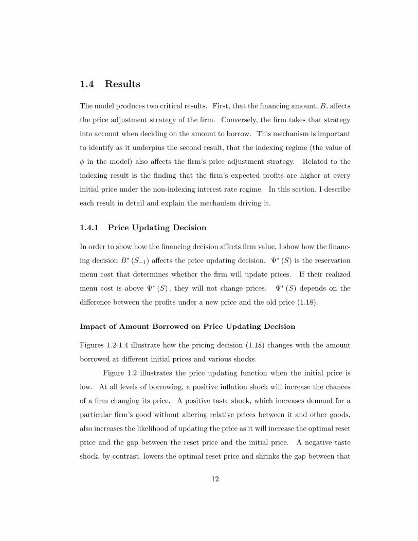
Figures 1.2-1.4 illustrate how the pricing decision (1.18) changes with the amount

borrowed at different initial prices and various shocks.

Figure 1.2 illustrates the price updating function when the initial price is

low. At all levels of borrowing, a positive inflation shock will increase the chances

of a firm changing its price. A positive taste shock, which increases demand for a

particular firm’s good without altering relative prices between it and other goods,

also increases the likelihood of updating the price as it will increase the optimal reset

price and the gap between the reset price and the initial price. A negative taste

shock, by contrast, lowers the optimal reset price and shrinks the gap between that

12

0 0.02 0.04 0.06 0.08 0.1 0.12 0.14 0.16 0.18 0.20

0.05

0.1

0.15

0.2

0.25

0.3

0.35

0.4

0.45

Amount Borrowed (Credit Limit)

Val

ue o

f ψ*

Influence of Credit limit on Price Decision, p-1 is 25%

inf -inf +taste -taste +

Figure 1.2: Impact of the amount borrowed on the reservation menu costwhen the initial price is low.

13

0 0.02 0.04 0.06 0.08 0.1 0.12 0.14 0.16 0.18 0.20

0.05

0.1

0.15

0.2

0.25

0.3

0.35

Amount Borrowed (Credit Limit)

Val

ue o

f ψ*

Influence of Credit limit on Price Decision, p-1 is 50%

inf -inf +taste -taste +

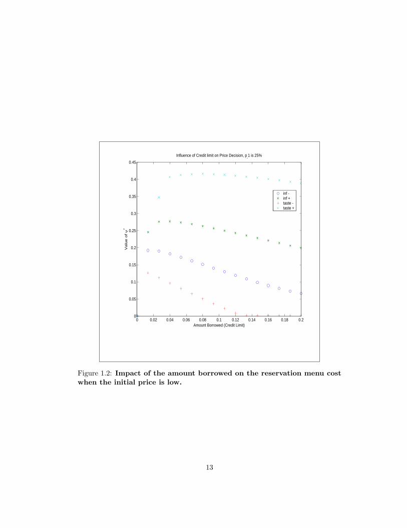
Figure 1.3: Impact of the amount borrowed on the reservation menu costwhen the initial price is close to optimal.

and the initial price, thus lowering the probability of a price change. Additionally,

note that as the borrowing amount increases, the probability of changing the price,

or alternatively, the benefit to changing the price, decreases. This increase in

borrowing raises qm (S) (1.9), and raises the value of a price change (1.18).

In Figure 1.3, the initial price is close to the unconstrained optimal (the

price the firm would choose in the absence of a cash in advance constraint or menu

costs). Notice here how the amount borrowed changes the value of updating the

price. When borrowing .06, there is no value to changing prices if the firm receives

14

0 0.02 0.04 0.06 0.08 0.1 0.12 0.14 0.16 0.18 0.20

0.02

0.04

0.06

0.08

0.1

0.12

0.14

Amount Borrowed (Credit Limit)

Val

ue o

f ψ*

Influence of Credit limit on Price Decision, p-1 is 75%

inf -inf +taste -taste +

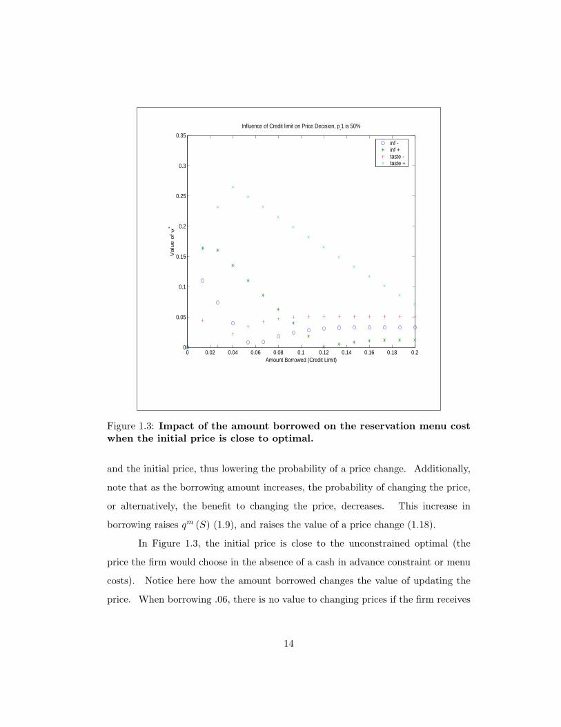
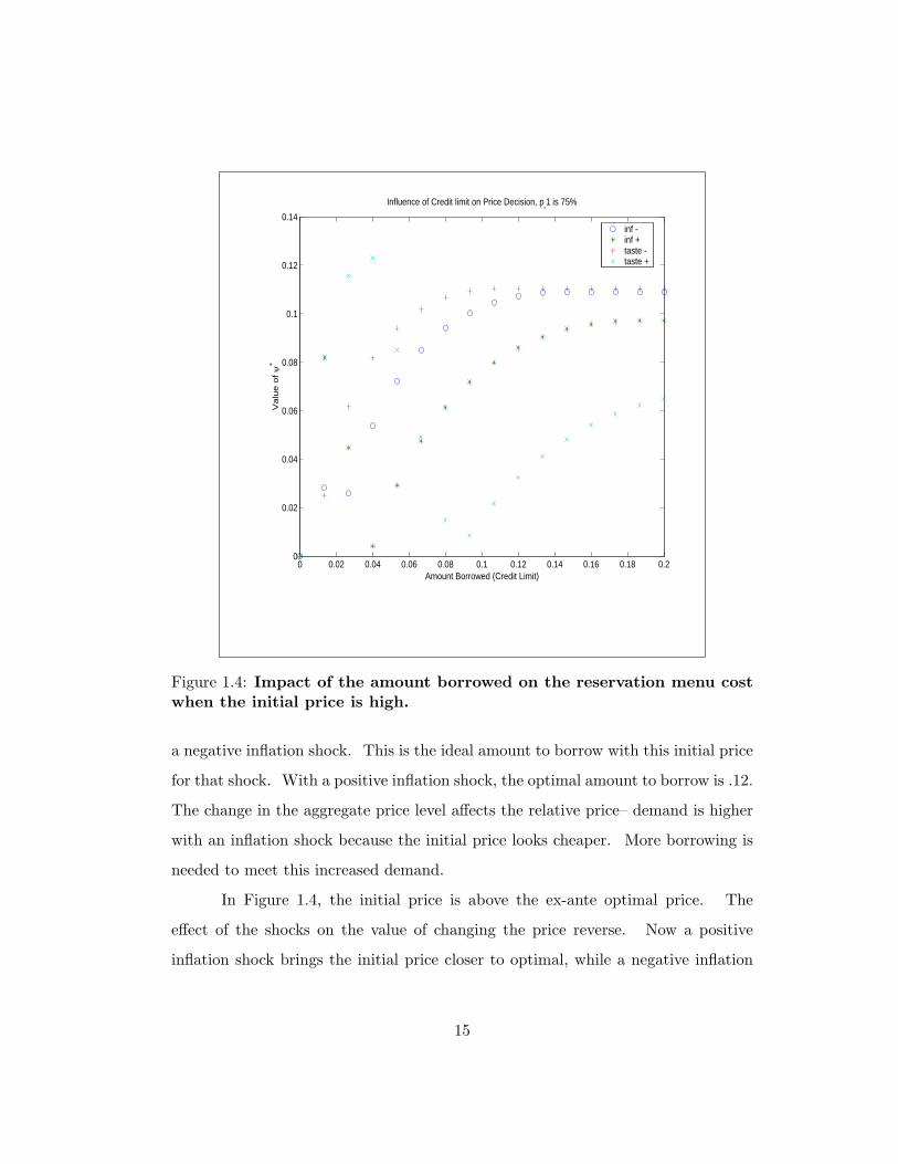
Figure 1.4: Impact of the amount borrowed on the reservation menu costwhen the initial price is high.

a negative inflation shock. This is the ideal amount to borrow with this initial price

for that shock. With a positive inflation shock, the optimal amount to borrow is .12.

The change in the aggregate price level affects the relative price– demand is higher

with an inflation shock because the initial price looks cheaper. More borrowing is

needed to meet this increased demand.

In Figure 1.4, the initial price is above the ex-ante optimal price. The

effect of the shocks on the value of changing the price reverse. Now a positive

inflation shock brings the initial price closer to optimal, while a negative inflation

15

shock moves it further way. A negative taste shock will reduce demand and make

our higher price closer to optimal, while a positive taste shock will do the opposite.

Additionally, borrowing more increases the value of changing price because any

change will be negative. If the firm is lowering its price to increase quantity, it has

to have borrowed enough to produce additional quantity.

Impact of Initial Price on Price Updating Decision

Figures 1.2-1.4 show how the impact that the amount borrowed has on the price

updating decision depends on the initial price. In order to capture the impact

of borrowing in a more systematic way, we can measure the impact of B on Ψ∗

when different constraints are binding. The amount borrowed creates an upper

limit on the quantity of goods that can be produced. This is represented by qm (S)

(1.9). If demand under the optimal unconstrained price is less than qm (S), then the

financing decision will not affect the expected profits in the change case. Similarly,

if demand under the previous price is less than qm (S), then the financing decision

will not affect profits in the no-change case. Thus, the marginal effect of a change

in financing on price adjustment and value needs to be evaluated for four separate

cases.

The borrowing constraint can affect the price and output decision even when

it doesn’t explicitly bind. I define the impact of the constraint as the difference in

the price and output in the realized second period compared to what the price and

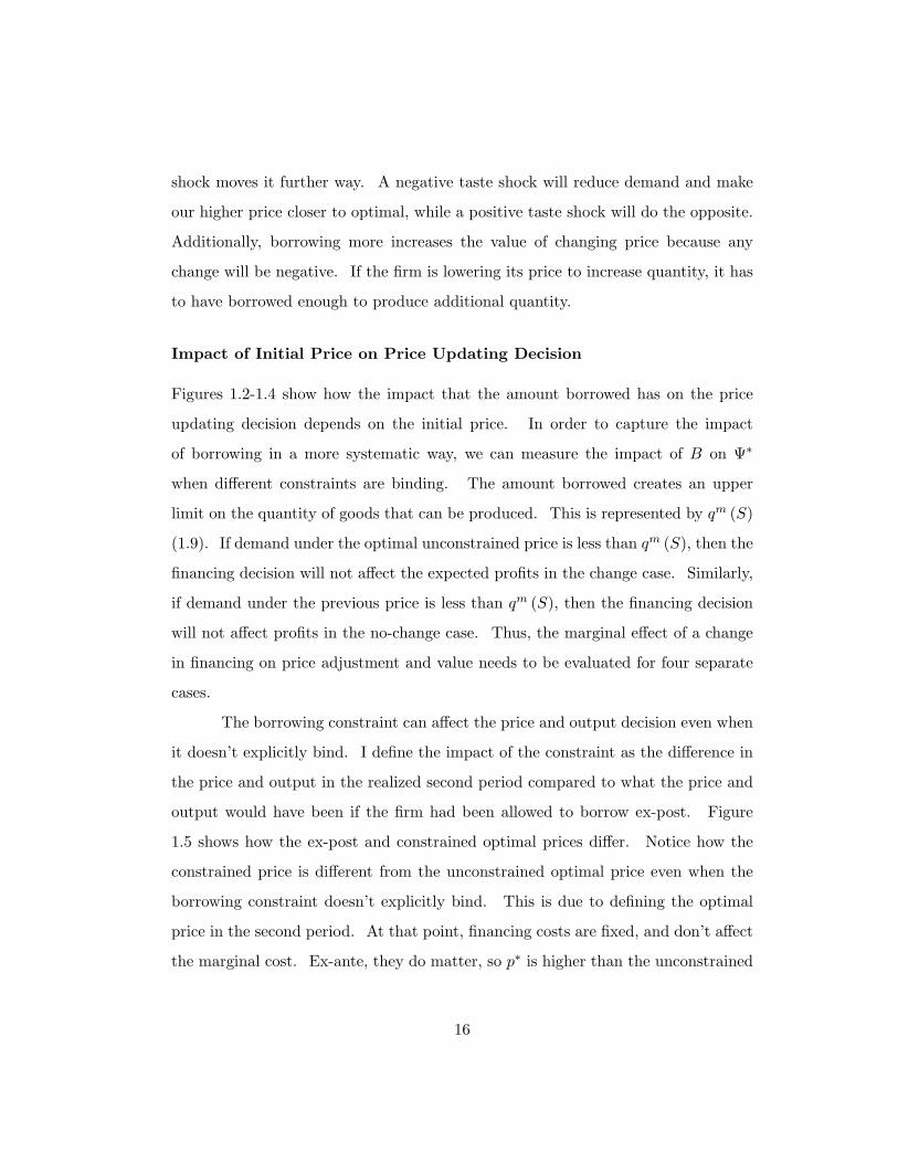
output would have been if the firm had been allowed to borrow ex-post. Figure

1.5 shows how the ex-post and constrained optimal prices differ. Notice how the

constrained price is different from the unconstrained optimal price even when the

borrowing constraint doesn’t explicitly bind. This is due to defining the optimal

price in the second period. At that point, financing costs are fixed, and don’t affect

the marginal cost. Ex-ante, they do matter, so p∗ is higher than the unconstrained

16

0 0.02 0.04 0.06 0.08 0.1 0.12 0.14 0.16 0.18 0.21.5

2

2.5

3

Amount Borrowed

Opt

imal

Pric

e

Effect of Debt on Price Policy in Change case

C-I-A Constrained Optimal PriceEx-Post Borrowing Optimal Price

Figure 1.5: Compare the optimal price conditioned on an amount borrowedwith an optimal price with ex-post borrowing., N = 3

optimal price (or alternatively, the ex-post borrowing optimal price), p∗unc when

the borrowing constraint is restrictive, but falls off as borrowing increases and the

constraint has less of an impact than the financing costs.

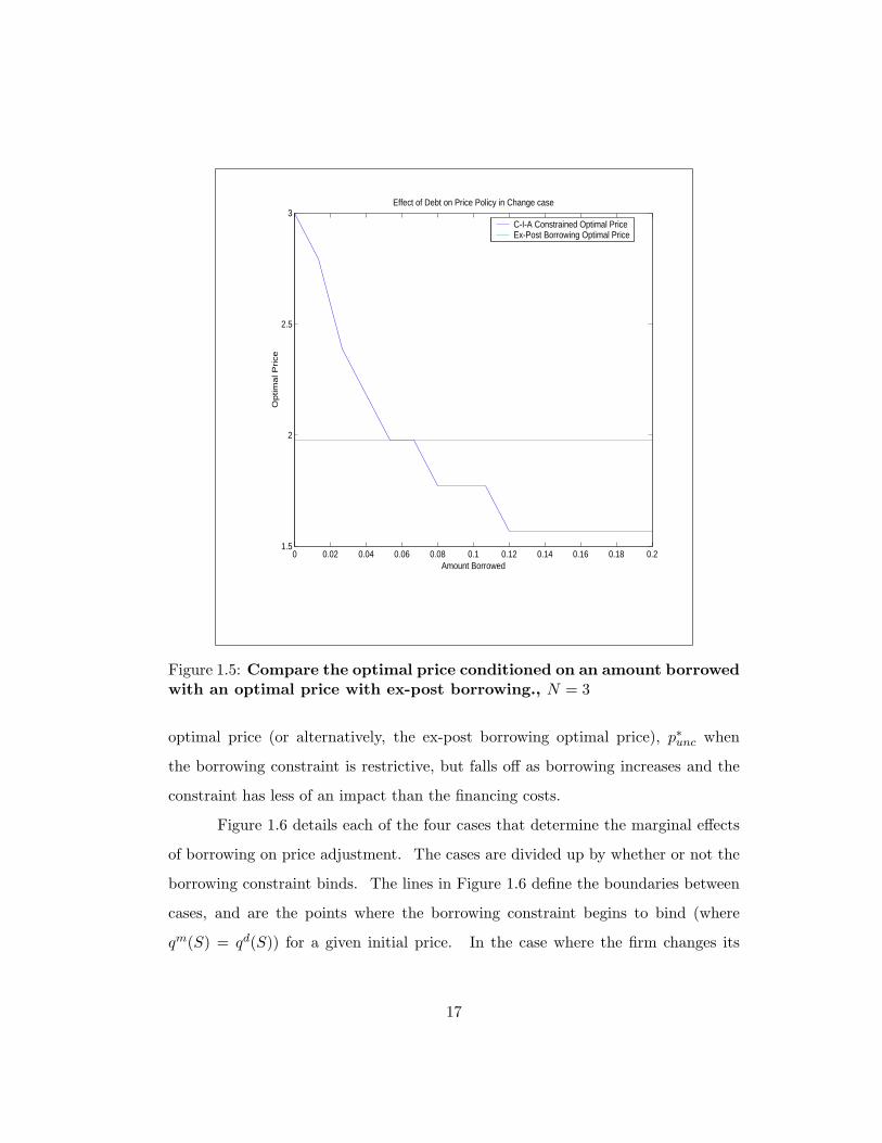
Figure 1.6 details each of the four cases that determine the marginal effects

of borrowing on price adjustment. The cases are divided up by whether or not the

borrowing constraint binds. The lines in Figure 1.6 define the boundaries between

cases, and are the points where the borrowing constraint begins to bind (where

qm(S) = qd(S)) for a given initial price. In the case where the firm changes its

17

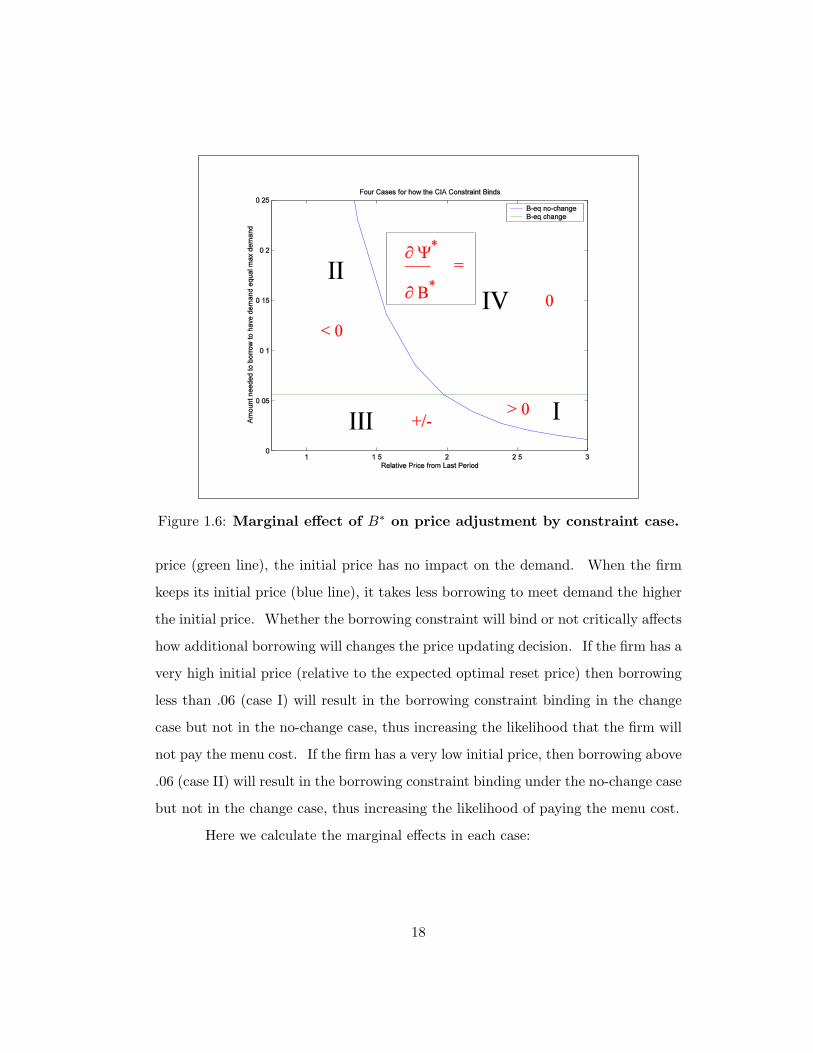
Figure 1.6: Marginal effect of B∗ on price adjustment by constraint case.

price (green line), the initial price has no impact on the demand. When the firm

keeps its initial price (blue line), it takes less borrowing to meet demand the higher

the initial price. Whether the borrowing constraint will bind or not critically affects

how additional borrowing will changes the price updating decision. If the firm has a

very high initial price (relative to the expected optimal reset price) then borrowing

less than .06 (case I) will result in the borrowing constraint binding in the change

case but not in the no-change case, thus increasing the likelihood that the firm will

not pay the menu cost. If the firm has a very low initial price, then borrowing above

.06 (case II) will result in the borrowing constraint binding under the no-change case

but not in the change case, thus increasing the likelihood of paying the menu cost.

Here we calculate the marginal effects in each case:

18

Case I: q(p∗unc) > qm (B) , q(p−1) ≤ qm (B)

Ψ∗ (S) = p∗(B

wP

)α

− p−1q(p−1)−B + wPq(p−1)1α

∂

∂BΨ∗ (S) =

∂p∗

∂B

(B

wP

)α

︸ ︷︷ ︸Price Falls

+αp∗

wP

(B

wP

)α−1

︸ ︷︷ ︸Quantity Rises

− 1︸︷︷︸Cost’s Rise

In case I, the borrowing constraint is binding in the change case but not in

no-change case. A firm that has a high initial price and borrows very little will

be in case 1. As the derivative is positive, we see that an increase in the amount

borrowed would increase Ψ∗, increasing the value to a firm of changing its price.

Case II: q(p∗unc) < qm (B) , q(p−1) ≥ qm (B)

Ψ∗ (S) = p∗q(p∗)− p−1

(B

wP

)α

− wPq(p∗)1α +B

∂

∂BΨ∗ (S) = −αp−1

wP

(B

wP

)α−1

+ 1

Case II describes the opposite situation, where the borrowing constraint does

not bind in the change case but does in the no-change case. Here the firm has a

very low initial price and has borrowed a lot. Borrowing more would lower the

value of changing price, as the firm would increase its price if it changes.

Case III: q(p∗unc) > qm (B) , q(p−1) > qm (B)

Ψ∗ (S) = p∗q(p∗)− p−1q(p−1)

∂

∂BΨ∗ (S) =

∂p∗

∂B

(B

wP

)α

+αp∗

wP

(B

wP

)α−1

︸ ︷︷ ︸Change Price

− αp−1

wP

(B

wP

)α−1

︸ ︷︷ ︸No Change

In case III, the constraint binds in both cases. It is unclear what effect an

increase in B would have on Ψ∗.

19

Case IV: q(p∗unc) ≤ qm (B) , q(p−1) ≤ qm (B)

Ψ∗ (S) = p∗q(p∗)− p−1q(p−1)− wP[q(p∗)

1α − q(p−1)

1α

]∂

∂BΨ∗ (S) = 0

Case IV is the unconstrained case. The firm has borrowed enough and has

a high enough initial price that additional borrowing will not affect its decision to

change its price or not.

The table below summarizes the how a change in B∗ (S) affects Ψ∗ through

each price changing scenario:

Table 1.1: Definition of Price Change and Borrowing Cases

Case q(p∗unc) q(p∗−1)

I q(p∗unc) > qm (B) q(p−1) ≤ qm (B)

II q(p∗unc) ≤ qm (B) q(p−1) > qm (B)

III q(p∗unc) > qm (B) q(p−1) > qm (B)

IV q(p∗unc) ≤ qm (B) q(p−1) ≤ qm (B)

Table 1.2: Summary of the Impact of Borrowing on Value

Case ∂∂BC Ψ∗ (θ) ∂

∂BNC Ψ∗ (θ) ∂∂BV (p∗) ∂

∂BV (p−1) ∂∂BV

I ∂p∗

∂B

(B

wP

)α + αp∗

wP

(B

wP

)α−1 − 1 0 + 0 +

II 0 −αp−1

wP

(B

wP

)α−1 + 1 0 + +

III ∂p∗

∂B

(B

wP

)α + αp∗

wP

(B

wP

)α−1 −αp−1

wP

(B

wP

)α−1 + + +/−

IV 0 0 0 0 0

Figure 1.7 shows how the marginal effects of each case change over different

levels of B for a given initial price. We can see that for low levels of borrowing, the

20

0

0.1

0.2

0.3

0.4Overall Effect: ψ* given B

0

5

10

15

ψ*

Marginal Effects: δψ*/δB p* Case

p-1 = 1.36

0 0.02 0.04 0.06 0.08 0.1 0.12 0.14 0.16 0.18 0.2-8

-6

-4

-2

0

Amount Borrowed

Marginal Effects: δψ*/δB p-1 Case

Figure 1.7: Marginal effects of additional borrowing on price adjustmentfor each price case given an initial price level.

change case is made more desirable with additional borrowings, and the no-change

case is made less so. This is consistent with case III, as both derivatives are non-

zero. At a critical amount of borrowing, the change case ceases to be affected by

additional borrowing. At this point, the change case borrowing constraint does

not bind. This is consistent with case II. The first panel of Figure 1.7 shows how

changes in B affect the overall value .

In the top of Figure 1.7 we see how the marginal effect of borrowing on

Ψ∗ changes as borrowings increase. At first it increases, as additional borrowings

21

Figure 1.8: Mapping figure 1.7 back into the constraint space.

make a price change more profitable, but that effect begins to slow, and eventually

stop altogether. The middle and bottom panels decompose the marginal effect into

the change case and the no-change case. The middle panel illustrates the effect

of borrowing on the no-change case. While positive, it quickly falls to zero as

the additional constraint stops binding. In the change case, additional borrowing

actually makes changing the price less desirable, as there are more financing costs to

cover. Figure 1.8 shows the same four-case space again, this time with our chosen

initial price shown explicitly. Figure 1.7 maps into Figure 1.8, as the marginal

effects of each level of borrowing change. Note that as borrowing increases the firm

crosses from case III to case II. The borrowing amount, .06, is the same as where

the no-change effect falls to zero in the middle panel of Figure 1.7.

22

0.5 1 1.5 2 2.5 30.05

0.055

0.06

0.065

0.07

0.075

0.08

Relative Price from Last Period

Bor

row

ing

Dec

isio

n

Optimal Borrowing

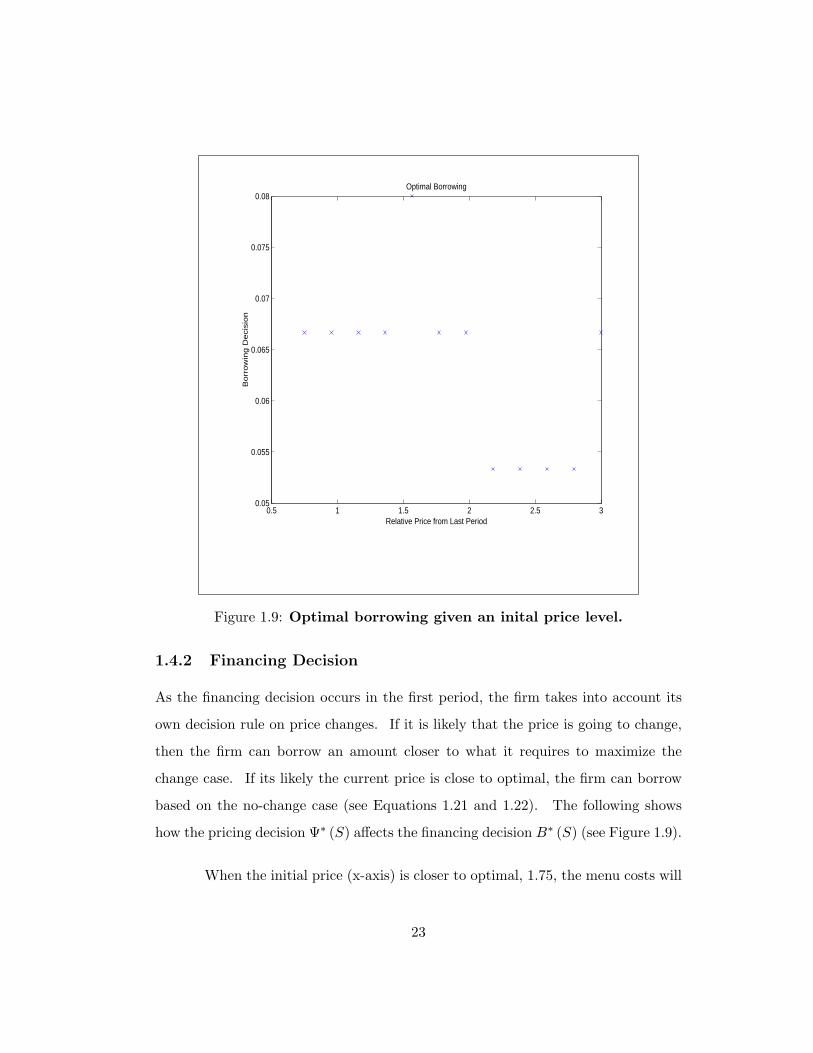
Figure 1.9: Optimal borrowing given an inital price level.

1.4.2 Financing Decision

As the financing decision occurs in the first period, the firm takes into account its

own decision rule on price changes. If it is likely that the price is going to change,

then the firm can borrow an amount closer to what it requires to maximize the

change case. If its likely the current price is close to optimal, the firm can borrow

based on the no-change case (see Equations 1.21 and 1.22). The following shows

how the pricing decision Ψ∗ (S) affects the financing decision B∗ (S) (see Figure 1.9).

When the initial price (x-axis) is closer to optimal, 1.75, the menu costs will

23

outweigh the benefit of changing the price and the firm will adjust its borrowing

to maximize under the initial price. Thus, the firm borrows more when the initial

price is below optimal, 1.5, in order to meet the higher demand. Conversely, they

can borrow less when the initial price is slightly too high, 2.1, to meet lower demand.

This process is limited by the magnitude of the menu cost however, and we can see

it break down at extreme initial price levels, 1 and 3. When the initial price is so

far away from the optimal that updating is a virtual certainty, the initial price has

little effect on borrowing and the firm borrows to maximize under its newly updated

price.

When faced with the borrowing decision, the firm knows the current price

level and its own price. This is enough for the firm to determine how far its current

price will deviate from the optimal price in the next period for each realization

of the shocks. The likelihood of updating the firm’s price is summarized in the

price change policy function. It is an important factor in the borrowing decision

because the optimal amount of borrowing depends on the demand. To see the

mechanism more clearly, separate the borrowing decision into two policy functions,

each conditional on a particular price updating strategy:

B∗C (S−1) = max{B}

∫S

ΠC (p, q, S) dS (1.21)

B∗NC (S−1) = max{B}

∫S

ΠNC (q, S) dS (1.22)

B∗C (S−1) is the optimal amount to borrow if the firm was changing its price

for sure, B∗NC (S−1) the amount if the firm was definitely not going to change its

price.

Now divide the second period into two states defined by the relative size of

the optimal amount to borrow for each price change scenario. If the initial price is

very low, a decision to raise it will reduce demand and require less borrowing. If

24

the initial price is very high, updating it will increase demand, and necessitate more

borrowing. Define these two situations as cases 1 and 2:

Case 1: B∗C (S−1) < B∗NC (S−1) (1.23)

Case 2: B∗C (S−1) ≥ B∗NC (S−1) (1.24)

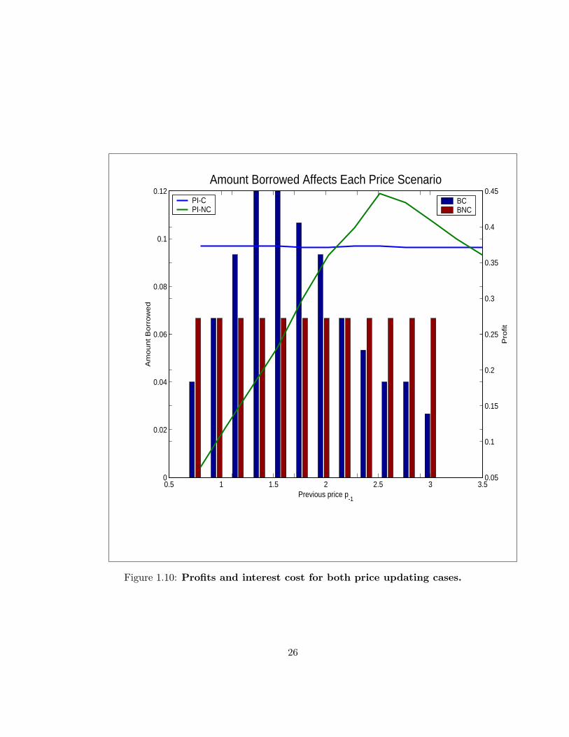
There are two channels through which the price change affects the borrow-

ing decision: the benefit of relaxing a binding cash-in-advance constraint, thereby

allowing supply to be optimal, and the cost of paying interest on the borrowing. In

case 1, these two channels reinforce each other; changing the price will move the firm

closer to first-best profits and also mean less borrowing and interest costs. In case

2, the two channels are at odds, as changing the price will yield greater efficiency

but also increased borrowing costs. Figure 1.10 illustrates these two mechanisms

across different values of the initial price.

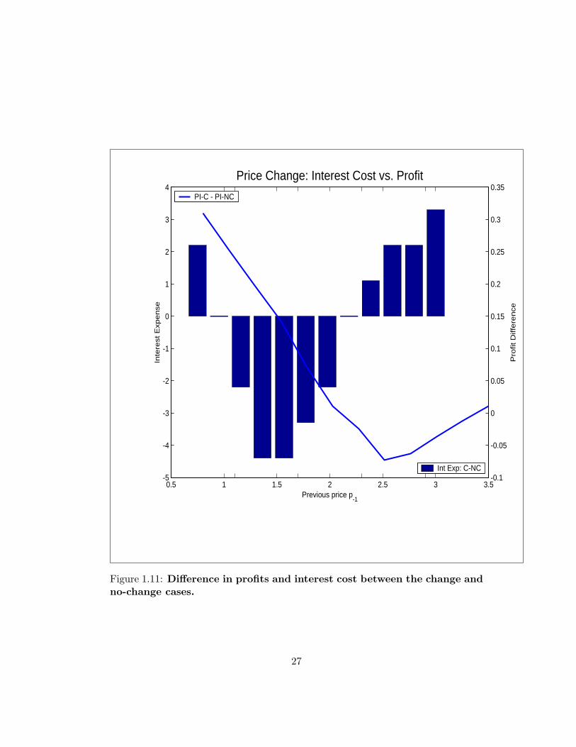
If we think of the reservation menu cost as the amount of inefficiency the

firm will accept before changing its price, then an increase in Ψ∗ tilts the borrowing

more towards the no-change optimum.

∂

∂Ψ∗B∗ (S−1) =

Case Interest Optimal Net Effect

1 − + +

2 − − −

Figures 1.11 illustrates the net effect.

1.4.3 Indexing Effects

We are now ready to consider the effects of indexing costs to inflation. If firms

choose to set φ greater than zero, then the interest rate will rise and fall with

inflation. Changes in λ, the wage indexation, were also considered but did not

affect the results presented here. While changes in λ impact profits and the policy

25

0.5 1 1.5 2 2.5 3 3.50

0.02

0.04

0.06

0.08

0.1

0.12

Previous price p-1

Am

ount

Bor

row

ed

BCBNC

0.05

0.1

0.15

0.2

0.25

0.3

0.35

0.4

0.45

Pro

fit

Amount Borrowed Affects Each Price ScenarioPI-CPI-NC

Figure 1.10: Profits and interest cost for both price updating cases.

26

0.5 1 1.5 2 2.5 3 3.5-5

-4

-3

-2

-1

0

1

2

3

4

Previous price p-1

Inte

rest

Exp

ense

Int Exp: C-NC-0.1

-0.05

0

0.05

0.1

0.15

0.2

0.25

0.3

0.35

Pro

fit D

iffer

ence

Price Change: Interest Cost vs. ProfitPI-C - PI-NC

Figure 1.11: Difference in profits and interest cost between the change andno-change cases.

27

0.6 0.8 1 1.2 1.4 1.6 1.8 2 2.2 2.4 2.60.484

0.486

0.488

0.49

0.492

0.494

0.496

0.498

Previous price p-1

Ex[

ecte

d P

rofit

Non-IndexedIndexed

4.2

4.4

4.6

4.8

5

5.2

5.4

5.6

5.8x 10-3

Diff

eren

ce in

Exp

ecte

d P

rofit

Expected Profits for Alternate IndexingDifference

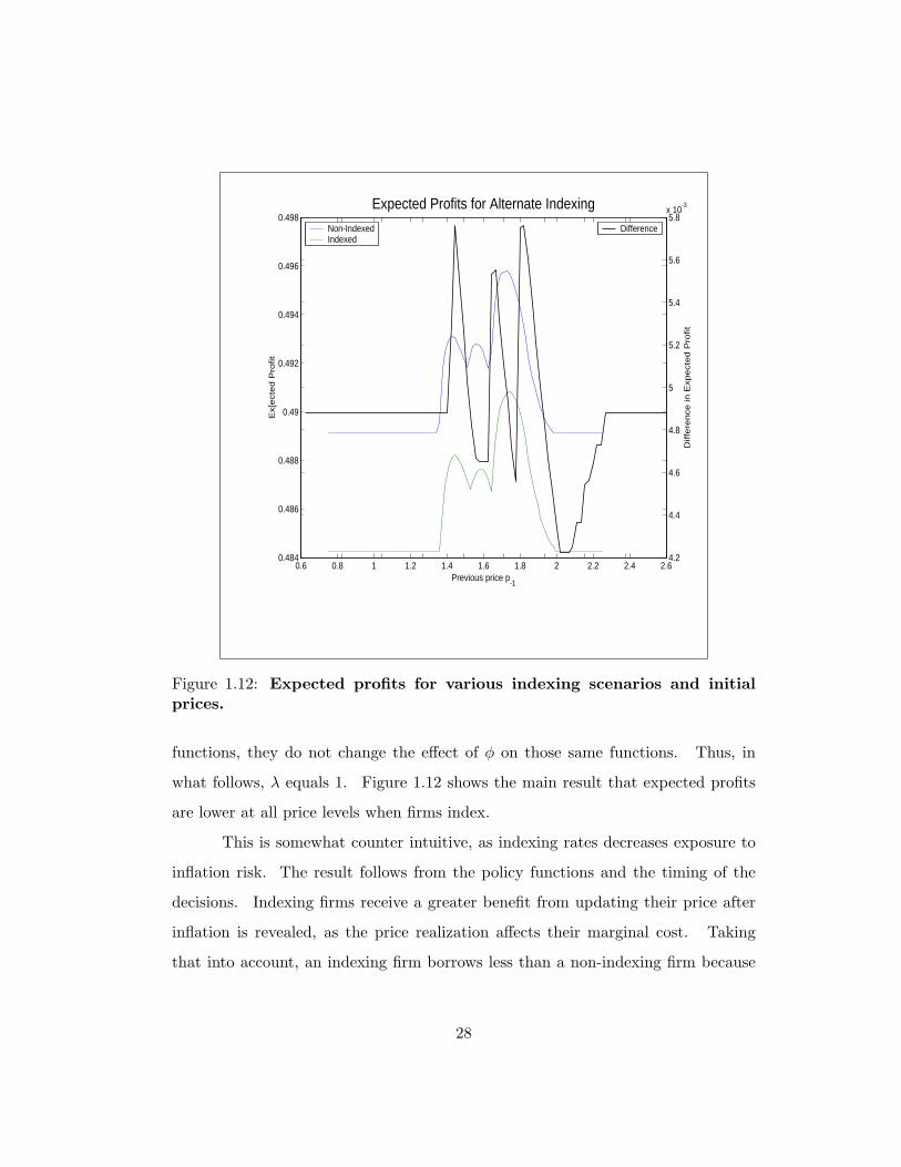
Figure 1.12: Expected profits for various indexing scenarios and initialprices.

functions, they do not change the effect of φ on those same functions. Thus, in

what follows, λ equals 1. Figure 1.12 shows the main result that expected profits

are lower at all price levels when firms index.

This is somewhat counter intuitive, as indexing rates decreases exposure to

inflation risk. The result follows from the policy functions and the timing of the

decisions. Indexing firms receive a greater benefit from updating their price after

inflation is revealed, as the price realization affects their marginal cost. Taking

that into account, an indexing firm borrows less than a non-indexing firm because

28

0.6 0.8 1 1.2 1.4 1.6 1.8 2 2.2 2.4 2.60.46

0.48

0.5

0.52

0.54

0.56

0.58

Previous price p-1

Rea

lized

Pro

fit

Non-IndexedIndexed

0.055

0.06

0.065

0.07

0.075

0.08

Diff

eren

ce in

Pro

fit

Realized Profits for Alternate Indexing (Inflation Shock)Difference

Figure 1.13: Realized profits for each indexation scenario when the tasteshock is zero and the inflation shock is positive.

it is less concerned about a low nominal price (1.24). This becomes a self fulfilling

result after price levels are realized. If inflation is positive, the indexed firm will

either have to change prices or produce less, because it did not borrow as much as

the non-indexing firm. Indexing firms manage their exposure to shocks by changing

price, whereas non-indexed firms manage these shocks by borrowing more.

To understand this result more clearly, consider the how each indexation

scenario preforms under the case of a positive inflation shock.

Figure 1.13 shows how the non-indexing firm does much better than the

29

0.6 0.8 1 1.2 1.4 1.6 1.8 2 2.2 2.4 2.60.42

0.43

0.44

0.45

0.46

0.47

0.48

0.49

0.5

0.51

Previous price p-1

Rea

lized

Pro

fit

Non-IndexedIndexed

-0.07

-0.065

-0.06

-0.055

-0.05

-0.045

Diff

eren

ce in

Pro

fit

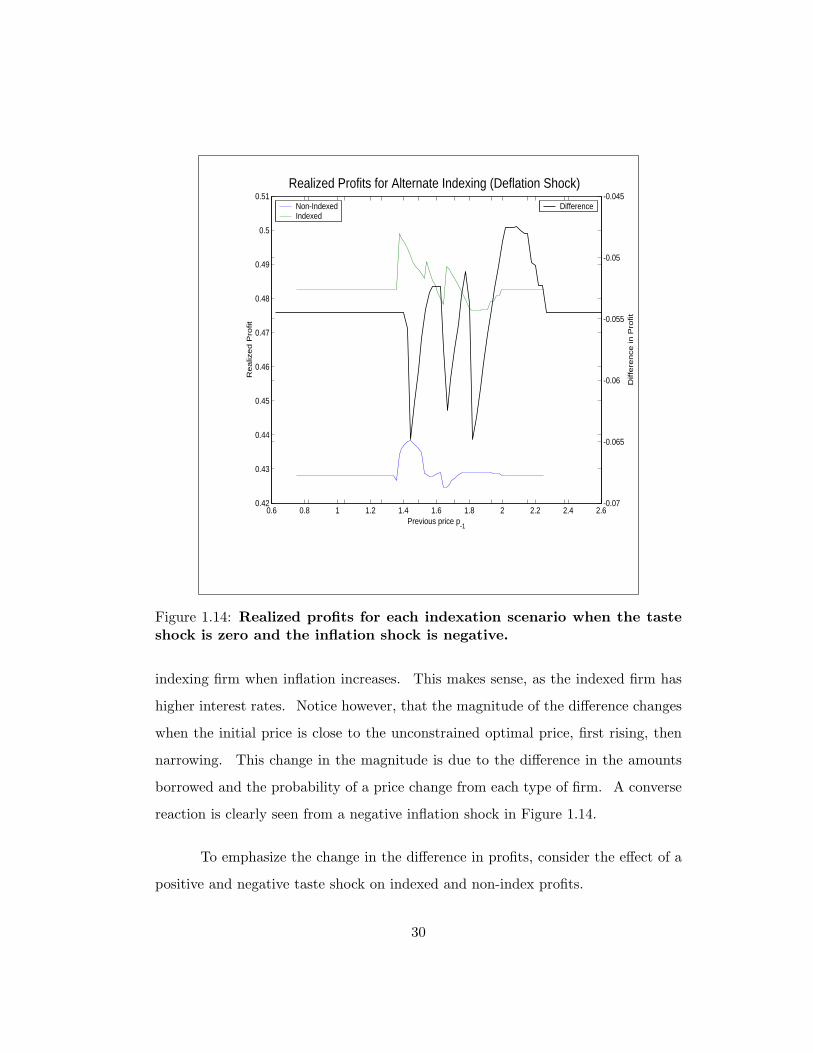
Realized Profits for Alternate Indexing (Deflation Shock)Difference

Figure 1.14: Realized profits for each indexation scenario when the tasteshock is zero and the inflation shock is negative.

indexing firm when inflation increases. This makes sense, as the indexed firm has

higher interest rates. Notice however, that the magnitude of the difference changes

when the initial price is close to the unconstrained optimal price, first rising, then

narrowing. This change in the magnitude is due to the difference in the amounts

borrowed and the probability of a price change from each type of firm. A converse

reaction is clearly seen from a negative inflation shock in Figure 1.14.

To emphasize the change in the difference in profits, consider the effect of a

positive and negative taste shock on indexed and non-index profits.

30

0.6 0.8 1 1.2 1.4 1.6 1.8 2 2.2 2.4 2.60.475

0.48

0.485

0.49

0.495

0.5

0.505

Previous price p-1

Rea

lized

Pro

fit

Non-IndexedIndexed

-0.01

-0.005

0

0.005

0.01

0.015

0.02

0.025

Diff

eren

ce in

Pro

fit

Realized Profits for Alternate IndexingDifference

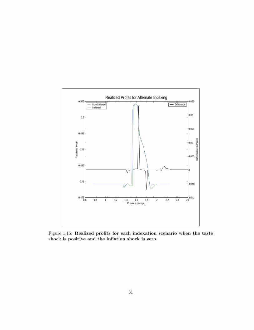
Figure 1.15: Realized profits for each indexation scenario when the tasteshock is positive and the inflation shock is zero.

31

0.6 0.8 1 1.2 1.4 1.6 1.8 2 2.2 2.4 2.6

0.503

0.5035

0.504

0.5045

Previous price p-1

Rea

lized

Pro

fit

Non-IndexedIndexed

-1.5

-1

-0.5

0

0.5

1

1.5x 10-3

Diff

eren

ce in

Pro

fit

Realized Profits for Alternate IndexingDifference

Figure 1.16: Realized profits for each indexation scenario when the tasteshock is negative and the inflation shock is zero.

Figure 1.15 shows the impact of a demand shock without a corresponding

change in indexed interest rates. This eliminates the large but fixed cost associated

with a higher interest rate bill. There is still a difference in profits right around the

critical optimal reset price, though it slightly favors the non-indexing firm. When

the price is close to the optimal reset price, the non-indexing firm borrows more,

which is an advantage under a positive demand shock. When the taste shock in

negative, as in Figure 1.16, the reverse is true, and the indexing firm does better.

The following example illustrates the asymmetry that leads the non-indexing

32

firm to higher profits. Firm I indexes its financing, while Firm N does not. Firms I

and N have the same initial price in period 1, which is lower than their ex-ante opti-

mal price. When considering how much to borrow, each firm assesses the likelihood

of changing its price. Figure 1.17 illustrates the differences in their assessment.

In the case of positive inflation, the firms have almost identical reservation menu

costs. The positive inflation shock exacerbates the gap between their initial price

and optimal price, and both firms will likely update their price. The case of a

negative inflation shock leads to a much different result. Firm I is willing to pay

a much higher menu cost to update its price. Because its financing is indexed, the

deflation changes the firm’s optimal reset price, moving it further from the initial

price. The deflation has no effect on Firm N’s as its optimal reset price as it is

independent of the price level. The deflation shock merely shrinks the gap between

its initial price and the optimal reset price.

After assessing the likelihood of updating their prices, the firms choose an

amount to borrow. This amount can be thought of as the weighted average of the

amount the firm would borrow if it were certain it was going to change its price and

the amount it would borrow if it were certain it would leave the price unchanged

(see Equations 1.21 and 1.22). Firm I is more certain that it will update its price,

so the amount it borrows will be more heavily weighted to B∗C . Since the initial

price is lower than the ex-ante optimal price, borrowing case 2 applies. In case 2,

B∗C is less than B∗NC , and any change in price will be an increase and will lower

the quantity demanded. Thus, Firm I borrows less than Firm N in this case.

Having made their borrowing decisions, the firms move into the second pe-

riod. In the case of positive inflation, both firms change their price and meet

demand. In that scenario, it is unclear who profits more. Firm I borrowed less

overall, but pays a higher interest cost due to the inflation. If there is negative

inflation, Firm I pays the menu cost and changes its price before Firm N. Firm I is

33

0.6 0.8 1 1.2 1.4 1.6 1.8 2 2.2 2.4 2.60.4

0.5

0.6

0.7

0.8

0.9

1

Relative Price from Last Period

Pro

babi

lity

of C

hang

ing

Pric

e

Probability of Changing Price for Various Indexing Scenarios

Non-Indexed BorrowingsIndexed Borrowings

Figure 1.17: Expected reservation menu cost for various indexing scenariosand initial prices.

more borrowing constrained than Firm N, and its optimal reset price is increasing.

In this case, Firm N comes out ahead, as it pays the menu cost less frequently.

Summing over all the states, it’s clear that the non-indexed firm is more profitable

than the indexed firm. The non-indexed interest rate helps affects the borrowing

decision by reducing the benefit to changing price and keeps the optimal reset price

fixed over both periods. The same asymmetries that drive the above example are

present in a situation where the initial price is higher than the optimal rest price

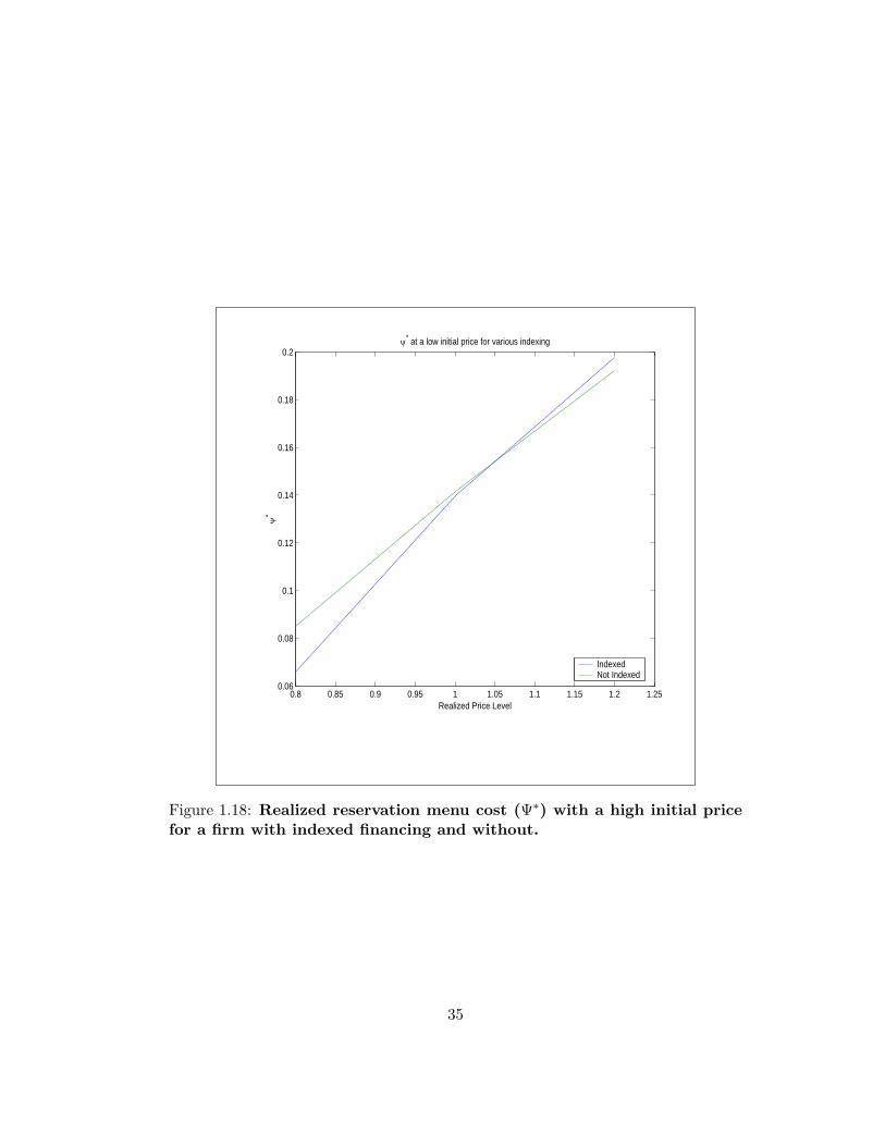
(see Figure 1.18).

34

0.8 0.85 0.9 0.95 1 1.05 1.1 1.15 1.2 1.250.06

0.08

0.1

0.12

0.14

0.16

0.18

0.2

Realized Price Level

ψ*

ψ* at a low initial price for various indexing

IndexedNot Indexed

Figure 1.18: Realized reservation menu cost (Ψ∗) with a high initial pricefor a firm with indexed financing and without.

35

0.8 0.85 0.9 0.95 1 1.05 1.1 1.15 1.2 1.250.04

0.05

0.06

0.07

0.08

0.09

0.1

0.11

0.12

Realized Price Level

ψ*

ψ* at a high initial price for various indexing

IndexedNot Indexed

Figure 1.19: Realized reservation menu cost (Ψ∗) with a low initial pricefor a firm with indexed financing and without.

36

1.5 Conclusion

This paper presents a model of the firm that incorporates state dependent pricing

and a cash-in-advance constraint. This simple framework illustrates how these two

inefficiencies work together to violate the irrelevance proposition and make a firm’s

financing an important factor in determining value.

I show that the cash-in-advance constraint affects both the price updating

decision and the optimal price if the optimal price in either the no-change or the

change case would require additional borrowing. In some cases this influenced the

new optimal price even when the cash-in-advance constraint didn’t appear to be

binding.

Additionally, I show that the type of interest rates alone affect price updating

behavior as well as expected profits. Firm’s paying interest rates indexed to infla-

tion borrowed less and updated their price more frequently, earning lower expected

profits. Financing costs under non-indexed rates move with inflation based demand

shocks. This allows firms to change prices more efficiently and earn higher expected

profits. These results depend critically on the assumption of positive menu costs.

If a firm could change its price costlessly, then there wouldn’t be an advantage to

borrowing at nominal rates.

As a next step in this investigation, I would like to estimate the nature of

the relationship between price stickiness and the degree of indexation in a firm’s

capital structure. I would expect to find the firms that change their price relatively

infrequently would have a high degree of indexation in their capital structure.

37

Appendix A. Parameter ValuesFor the policy functions shown in the paper the following parameter values

were used:

α

γ

β

Ψ

D

w

µ

P−1

rF

λ

φ

=

0.5

1.9

.99

[0, 0.025]

1

.75

(.5, 1.5)

1

0.2

{0, 1}

{0, 2}

description:

Returns to scale

Price elasticity

Discount rate

Menu cost

Money Balance (hh)

Real Wage

Taste shock

Initial price level

Risk Free Rate

Amount Indexing

Interest Rate Indexing

38

Chapter 2

Asset Prices and Money in a

Two-Period Equilibrium

2.1 Introduction

Observers of public securities markets have often documented a level of price volatil-

ity that is much higher than justified by our current understanding of fundamental

value. In attempting to explain this anomaly, liquidity demands have frequently

been proposed as an explanation. If every trade were motivated by new information

about the fundamental value of an asset, we would expect much smaller moves in the

price. However, if some of the trades were motivated simply by a desire to convert

the asset into consumption, price fluctuations could be explained by differences in

agents’ desire to consume or save at a specific point in time.

This paper uses a Diamond and Dybvig (1983) style liquidity model to show

how the money supply relative to the supply of productive assets can affect asset

prices and asset price volatility. The model shows that higher levels of money

relative to assets will result in lower volatility for the price of the asset.

The link between asset price volatility and liquidity has been approached

39

using several modeling techniques. One method of obtaining excess volatility and

increased risk premium is to assume a fixed cost of participation. Models utilizing

this have linked market liquidity to both high and low levels of volatility. Pagano

(1989) uses participation costs to create endogenously thin markets. The thinness

of the market contributes to volatility though the number of agents. The fewer

the number of agents, the greater the impact of idiosyncratic liquidity shocks. The

expected increase in volatility due to idiosyncratic shocks feeds back into the par-

ticipation decision, multiplying the impact of an initial shock on volatility. Orsel

(1995) uses a similar model to Pagano but generates an increase in volatility due to

participation. In his model, the marginal participant only enters after observing a

positive signal about returns. This agent will have the highest cost to participate,

so will accept the largest liquidity cost. Thus, increased participation is correlated

with high level of volatility. Dubra and Herrera (2001) generates a similar result,

using the marginal risk aversion of the agent instead of a signal.

Allen and Gale (1994) model asset price volatility using a Diamond and

Dyvbig style asset market. They introduce a fixed cost of participation to buy the

illiquid asset and uncertainty about the payoff of the asset. The Allen and Gale

model is remarkable in its ability to generate liquidity-based asset price volatility

without the use of thin markets, as in Pagano. At all times, assets and money are

costlessly exchanged. The changes in the level and volatility of the price are driven

solely by agents’ evolving demand for liquidity.

This paper follows the Allen Gale approach of assuming thick markets with

two innovations. First, while I include a liquidity demand shock as in Diamond

and Dyvbig, I also add a supply shock that alters the total supply of money in the

second period. This shock is known to agents in the initial period. I conclude

that shocks to the money supply increase the mean price level of the asset, and

decrease the price volatility. Secondly, I simplify the model by removing the fixed

40

cost of participation. While this innovation has been used to generate excessive risk

premia, I show that it is not necessary to establish the interaction between liquidity

and price volatility in this framework.

In the model, the volatility of the asset price is determined by the relative

value of the liquidity price of the asset, which is determined by the relative supply

of money and the asset at a point in time, and the fundamental value price of

the asset, which is determined by its return if held to maturity. If the liquidity

price is uncertain, the distribution of expected realizations of the price will have

an upper bound at the fundamental value; no one holding money would take a loss

for the privilege of holding the asset. The more of the liquidity price distribution

is truncated by the fundamental value price, the lower the overall volatility of the

price.

Section two presents the household problem in general terms and defines an

equilibrium. Section three derives explicitly policy functions to solve the household

problem and satisfy the equilibrium conditions. Section four utilizes comparative

statics to address the impact of liquidity on asset prices, demand and volatility.

Section five concludes.

2.2 Model

The model follows a simplified version of the Allen Gale portfolio problem. House-

holds face a choice in the initial period of allocating wealth between two assets,

while under uncertainty about which of the remaining two periods they will need to

consume. The model solution is partial equilibrium in the sense that its scope is

limited to the choice of asset allocation; I abstract from specific consumption and

production processes. The liquid asset (money, m) yields no return but can be used

for consumption in either the first or second period. The illiquid asset (“the asset”,

a) yields a positive real return (r), but is only realized in the second period. Money

41

is assumed to be the numeraire good, with consumption denominated in terms of

money. This allows us to avoid a separate aggregate price level between goods and

money. The only price in the model relates to the exchange between money and

assets. Agents face both idiosyncratic and aggregate uncertainty about whether

they are will be early or late consumers. Their liquidity needs will be determined

by an individual draw of a random variable λ. The distribution of λ is partially

revealed; the standard deviation is known, but the mean of the distribution is itself

a random variable (ν). This compound uncertainty creates both idiosyncratic risk

for a consumer about his or her demand timing, and also creates aggregate uncer-

tainty about fraction of total consumers who will consumer early or late. In the

first period, after the liquidity preference shock is revealed, there is a market for

early consumers to sell illiquid assets to late consumers. The aggregate uncertainty

about the distribution of λ creates uncertainty about the market clearing price of

the asset in the first period.

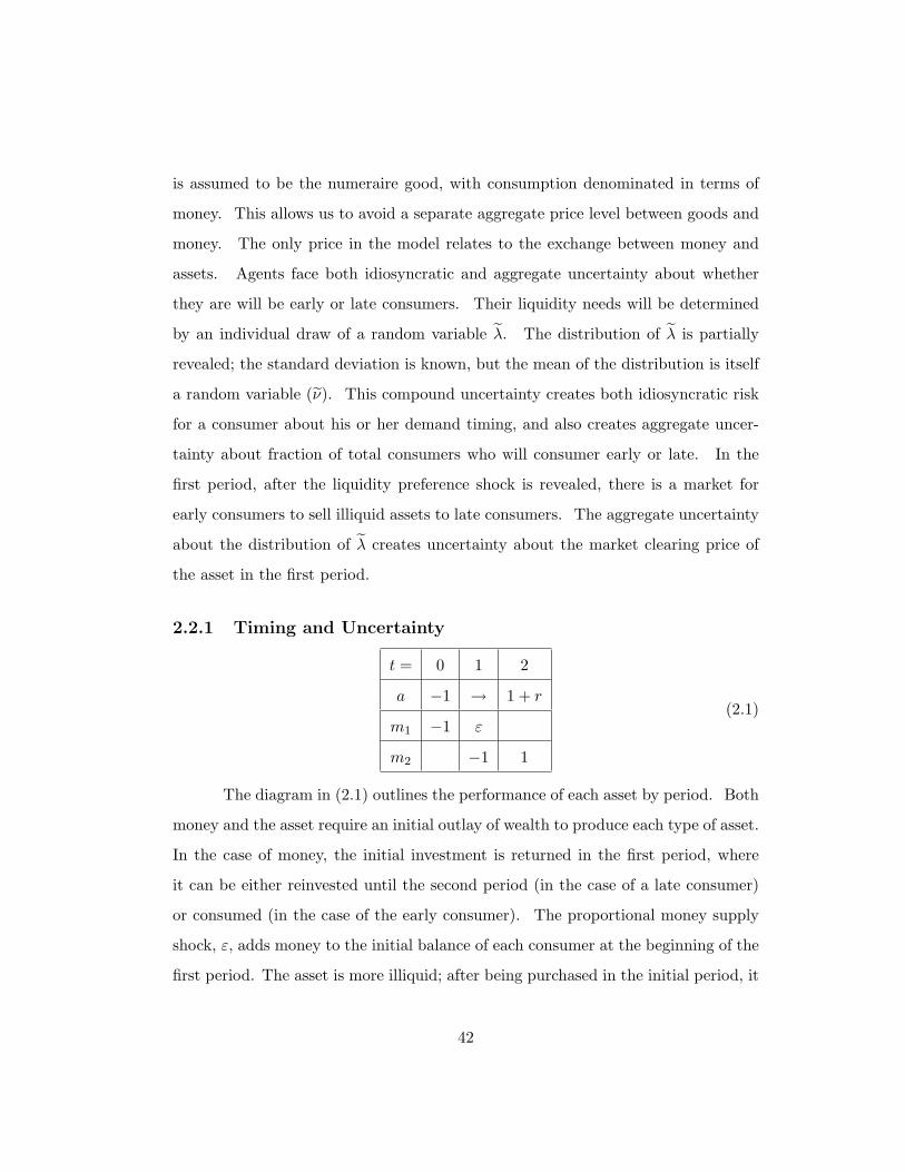
2.2.1 Timing and Uncertainty

t = 0 1 2

a −1 → 1 + r

m1 −1 ε

m2 −1 1

(2.1)

The diagram in (2.1) outlines the performance of each asset by period. Both

money and the asset require an initial outlay of wealth to produce each type of asset.

In the case of money, the initial investment is returned in the first period, where

it can be either reinvested until the second period (in the case of a late consumer)

or consumed (in the case of the early consumer). The proportional money supply

shock, ε, adds money to the initial balance of each consumer at the beginning of the

first period. The asset is more illiquid; after being purchased in the initial period, it

42

cannot be consumed in the first period. However, the asset returns all of the initial

investment in the second period plus the return r.

In the initial period, households make their allocation decision without know-

ing their liquidity preference. This allocation is accomplished through a constant

returns to scale process for both the money and the asset. Thus, the total supply

of money and the asset is determined by the agents’ initial period assessment of

their individual liquidity needs. The liquidity shock is revealed in the first period,

after which the agents attempt to reallocate between money and the asset. Con-

sumption occurs after that reallocation in the first period for early consumers. Late

consumers wait until the second period when the asset and its return converts to

consumption.

The liquidity shock creates both idiosyncratic and aggregate uncertainly. For

household i, the liquidity preference is determine by its draw of λi :

if λi ≥ 0, z = 1

if λi < 0, z = 0

λi is drawn from a normal distribution, where the standard deviation is known to

the households but the mean is not:

λ ∼ N (υ, σ) (2.2)

v ∼ N (ν, 1) (2.3)

The expected mean of the liquidity preference distribution, ν, is know to the con-

sumers in the initial period. Similarly to ε, it will act as a policy parameter and

define the space over which we investigate the changes to the price of the asset and

the volatility of that price.

43

2.2.2 Household Problem

The household essentially faces an optimal insurance problem. If a late consumer

knew his type in the initial period, he would allocate all his wealth to the asset and

earn the superior return. An early consumer would allocate all his wealth to money,

as the asset would be worthless to him. Thus, an allocation to money is insurance

against early consumption. This feature matches a critical aspect of liquidity in

general; the value of liquidity is the ability to access wealth at any time, without

necessarily knowing ahead of time if it will be needed. The premium agents pay

for this insurance is the opportunity cost of a higher return on the less liquid asset.

Stated formally, the household solves the following problem:

V (wi, ε, v, r) = maxci1,ci2

Ez,λ [u (ci1, ci2)] s.t. (2.4)

ci1 ≤ mi0ε+mi1 (2.5)

ci2 ≤ mi0ε+mi1 + (1 + r) (ai0 + ai1) (2.6)

wi ≥ mi0ε+ p0ai0 (2.7)

p1ai1 −mi1 = 0 (2.8)

ai0,mi0ε ≥ 0; ai1 ≥ −ai0, mi1 ≥ −mi0ε, (2.9)

The household attempts maximizes its total utility in each allocation period.

In the first period, it chooses ci1 and ci2 knowing there is a chance it could consume

either early or late.

u (ci1, ci2) =

u (ci1) if z = 1

u (ci2) if z = 0

(2.10)

This choice is subject to a cash-in-advance constraint for each consumption

period (2.5, 2.6) and a budget constraint for each period (2.7, 2.8). Additionally, I

impose a restriction on short selling and net borrowing (2.9).

44

In order to get some meaningful intuition on the comparative statics, and to

attempt a more rigorous answer to the questions posed by the paper, I assume the

following quadratic form to the utility function:

u (c) = c− b

2c2 (2.11)

Any well behaved utility function (continuous, differentiable, u′ (·) > 0,

u′′ (·) < 0) will yield similar results.

2.2.3 Market Clearing

As in the Allen Gale model, the allocation decision in the initial period is actually

a production decision, as agents transform wealth into money and the asset. This

process endogenizes the entire of supply of assets and money in the initial period.

The money supply shock, ε, is applied to balances in the first period, but known to

the agents in the initial period.

∑i

ai = A; ε ·∑

i

mi = M (2.12)

First period market clearing involves only a subset of the total supply of

money and assets. Late consumers who hold assets and early consumers who hold

money will not offer them for exchange as the assets will be held and consumed,

respectively. Thus, the first period market is made up of assets held by early

consumers and money held by late consumers. The proportion of each type can be

determined from the realization of the mean of the λ distribution (ν)

z∗ = Pr(λi ≥ 0|ν = ν) (2.13)

z∗ informs the fraction of total assets and money that are being traded in

45

period 1.

∑i

p1aEi =

∑i

mLi

z∗p1A = (1− z∗)M (2.14)

Its not strictly correct to say that p1 will clear the market for assets in period

1. There are several corner solutions where the market does not clear. In period

1, the asset has a guaranteed return of 1 + r in the next period. Those selling the

asset will be unable to charge more than 1 + r for it no matter how strong the

demand is for late consumption. That is, p1 will be the lesser of either the market

clearing price. or 1 + r. This difference between the market clearing price, which

I referred to in the introduction as the liquidity price, and the true value of the

asset, the fundamental value price, drives the volatility result. If those prices are

close together in expectation, the distribution of the liquidity price will be truncated

more severely than if they’re further apart. The more the distribution is limited,

the lower the volatility.

2.2.4 Equilibrium

Define a set of parameters S = {w, ε, v, r} . An equilibrium for this model is defined

as a series of policy functions a0 (S) , m0(S), aE1 (p1) , mE

1 (p1) , aL1 (p1) , mL

1 (p1)

that solve the household problem (2.4) subject to the constraints (2.5-2.9) and a

price, p1, that clears the market in period 1 (2.14). The next section will use the

assumed functional form of demand to develop a solution for the equilibrium, and

derive expressions for the expected price and volatility of the first period asset.

46

2.3 Solving the Model

The household faces two sequential decisions, with the second depending critically

on the first. The solution to the household’s problem begins in the first period

and works back to the initial allocation. In what follows, I have dropped the ”i”

subscripts on the policy functions, as the only difference between consumers is their

ex-post type, which is labelled where appropriate.

2.3.1 First period (t = 1)

At the beginning of the first period, the household has already allocated its wealth

between money and assets. At the time of the allocation, the household did not

know if it would be an early or late consumer; liquidity preference is revealed at

the start of the first period. Thus, while in the initial period our agents were

homogenous, the first period sorts them into two groups, early and late consumers,

who each solve a separate problem.

Early Consumer

Early consumers experience utility from consuming in the first period, but none

from consuming in the second, when the asset pays off.

u(c1, c2; z = 1) = maxa1,m1

1 · u(c1) + 0 · u(c2)

c1 ≤ m0ε+m1

c2 ≤ m1 + (1 + r) (a1 + a2)

Thus, the early consumer will want to exchange his asset holdings for money in

order to maximize his current period consumption and overall utility. Substituting

the first period budget constraint (2.7), which we can assume will bind, into the

household problem (2.4), the early consumer will have the following demand for

47

money and assets:

mE∗1 = p1a0 (2.15)

aE∗1 = −a0 (2.16)

The market will always clear for the early consumer, as they will accept any

price for their initial asset allocation.

Late Consumer

Late consumers experience utility from consuming in the second period, when the

asset pays off and returns the initial investment plus the return in terms of con-

sumption. In the first period, upon learning that they are late consumers, these

households no longer have a need to insure against early consumption, and would

like to put the wealth that they allocated towards money in the initial period (m0)

to a more productive use, i.e., buy the asset. Rewriting the early consumer problem

to account for z = 0 :

u(c1, c2; z = 0) = maxa1,m1

0 · u(c1) + 1 · u(c2) (2.17)

c1 = m0ε+m1 (2.18)

c2 = m0ε+m1 + (1 + r) (a0 + a1) (2.19)

The late consumers problem is slightly more complex than the early consumer’s.

By substituting the second period budget constraint (2.8) into (2.19), we can write

48

the late consumers problem as a Lagrange maximization:

L(a,m, µ) = maxa1

m0 − p1a1 + (1 + r) (a0 + a1)− µ [m0ε− p1a1]

FOC :∂L

∂a1: −p1 + (1 + r) + µp1 = 0

µ : m0ε− p1a1

µ [m0ε− p1a1] ≤ 0

Unlike the early consumers, for whom the allocation to assets in the initial period

is now worthless if the hold onto it, late consumers value their money holdings to

the extent they can hold them until the second period. Where the early consumers

would accept any p1 ≥ 0, late consumers are only willing to pay p1 ≤ 1+r, the price

where they are indifferent between holding money and the asset. That is, when the

liquidity price is less than or equal to the fundamental value price.

Case 1: p1 ≤ 1 + r , µ > 0 (2.20)

Case 2: p1 > 1 + r , µ = 0 (2.21)

Therefore, the demand for the asset depends on the price:

aL∗1 =

m0εp1

if µ > 0

0 if µ = 0

(2.22)

Thus, by the first period budget constraint (2.7):

mL∗1 =

−p1a1 if µ > 0

0 if µ = 0

(2.23)

49

Market Clearing

Early consumers are natural buyers of money, late consumers will demand assets

as long as the price is not above the fundamental value of the asset, 1 + r. From

the market clearing condition (2.14) we can derive an expression for the first period

price:

p1 = min{

1− z∗

z∗M

A, 1 + r

}(2.24)

The late consumers each demand aL∗1 . They are willing to exchange all of the

money holdings, and there are a total of 1−z∗ of them. Conversely, early consumers

each demand mE∗1 , and there are z∗ of them (2.15 and 2.13). The distribution of

the expected realization of p1 in period 0 will be negatively skewed, as any value of

z∗ that yields a price above 1 + r will be truncated to 1 + r. For every realization

of the shock where the true value dominates, the price equals the true value. This

discrete choice drives the key result that volatility decreases as liquidity increases.

The more states yield market clearing prices above 1 + r, the more the distribution

is truncated, and the lower the volatility.

2.3.2 Initial Period

In contrast to the first and second periods, agents in the initial period do not know

whether they will be consuming earlier or later, and thus all face the same prob-

lem. Agents solve the household allocation problem by taking expectations over the

probability of drawing an early or late liquidity preference and the expected mean

of that distribution.

2.3.3 Household Problem

Rewrite the household problem (2.4) after substituting in the demand functions

from the first period (2.15, 2.22). As each consumption period is exclusive to the

50

other, c1 is optimized assuming an early liquidity preference, c2 assuming a late

liquidity preference.

V (wi, ε, v, r) = maxc1,c2

∫ν

∫λ[λu (c1) + (1− λ)u (c2)] dλdν (2.25)

c1 = m0ε+mE∗1 (p1) (2.26)

c2 = (1 + r)(a0 + aL∗

1 (p1))

if µ > 0 (2.27)

c2 = (1 + r) a0 +m0ε if µ = 0 (2.28)

Substituting in the budget constraint (2.7), the expectation of p1 (2.24) and

the specific demand functions in for c1 and c2 yields the following first order condition

for each λi and υ realization:

∂V

∂a0: −λ (1− p1)u′ (c1) + (1− λ)u′ (c2) (1 + r)

(1− 1

p1

)= 0 (2.29)

If we assume quadratic utility (2.11), demand in the initial period is a function of

the parameters and the shocks:

a∗0 = g (wi, ε, v, r) (2.30)

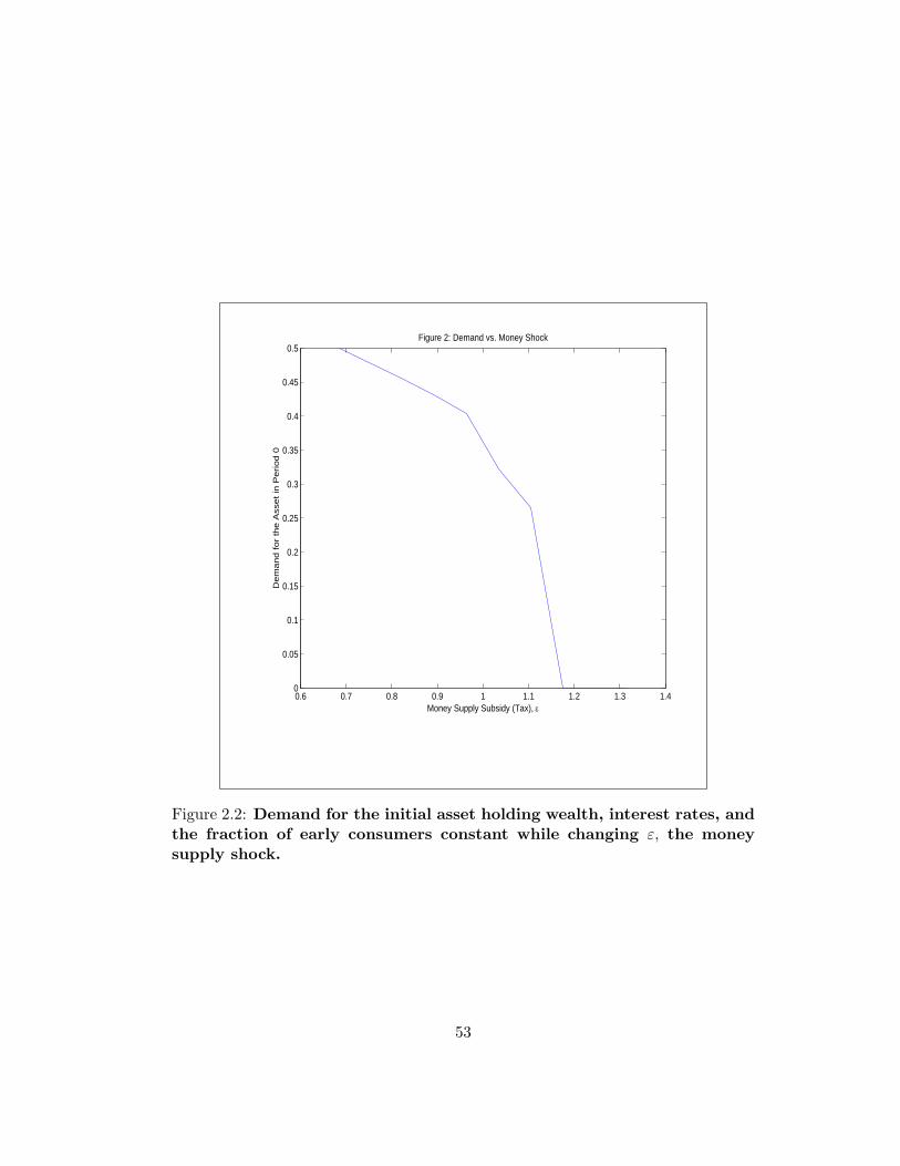
Figure’s 2.1 and 2.2 show how demand for the asset changes with the expected

fraction of early consumers and with the money shock.

Demand for the asset falls off as liquidity demand increases, as agents find

money to be more valuable relative to the asset as the chance of consuming early

increases. As the money shock increases, the return for owning money increases

and eventually overtakes the return on the asset. Hence zero demand for the asset

when ε is above 1.17.

51

0.44 0.46 0.48 0.5 0.52 0.54 0.56 0.58 0.60.41

0.42

0.43

0.44

0.45

0.46

0.47

0.48

0.49

0.5

Expected Mean of z*

Dem

and

for

the

Ass

et in

Per

iod

0

Figure 1: Demand vs. z*

Figure 2.1: Demand for the initial asset holding wealth, interest rates, andthe money supply shock constant and changing z∗, the fraction of peopleconsuming early.

52

0.6 0.7 0.8 0.9 1 1.1 1.2 1.3 1.40

0.05

0.1

0.15

0.2

0.25

0.3

0.35

0.4

0.45

0.5

Money Supply Subsidy (Tax), ε

Dem

and

for

the

Ass

et in

Per

iod

0

Figure 2: Demand vs. Money Shock

Figure 2.2: Demand for the initial asset holding wealth, interest rates, andthe fraction of early consumers constant while changing ε, the moneysupply shock.

53

2.3.4 Initial Price, p0

While there is no exchange occurring in the initial period, the allocation decision

that the households are making implicitly requires an expectation of the price of

assets in terms of money in period 1 (demand equation 2.15). This expectation

can be calculated as a shadow price in order to explore the implications of shocks

to liquidity demand (υ) and shocks to the aggregate stock of money (ε), to that

shadow price.

p0 = p1 (z∗ (ν)) (2.31)

p0 = E [p1] =∫

νp1 (z∗ (ν)) dv

The mean and variance of p0 are calculated based on the market clearing

price at each and every possible realization of ν. The expected value of p1 is:

E [p0] = min{

1− z∗

z∗M

A, 1 + r

}= µp (2.32)

The exists a value of z such that 1−zz

MA = 1 + r :

z =M

A (1 + r) +M(2.33)

Thus, the variance of the truncated distributions is:

V ar [p0] =∫ z

0(1 + r − µp)

2 dz +∫ 1

z

(1− z∗

z∗M

A− µp

)2

dz (2.34)

An increase in MA will affect variance through two channels. On the intensive

margin, it will increase the variance of the of p1 for values below (1 + r). On the

extensive margin, it will increase the mean of the distribution and move a higher

portion of it into values above (1 + r), where the variance is very small.

54

2.4 Results

In order to asses the impact of liquidity demand and liquidity supply on the shadow

price, I show a series of comparative statics on the mean and variance of p0. This

exercise shows unambiguously how an increase in liquidity will raise the price of the

asset. The volatility of the price of an asset declines as the money shock increases,

and increases with liquidity demand. Additionally, in order to provide a theoretical

link between this model and the empirical measure used in chapter 3, I define the

monetary services index in the context of this model. An alternate to a more

traditional measure of aggregate liquidity (M), I show how the total expenditure of

monetary services is in fact of measure of illiquidity.

2.4.1 Impact of liquidity shocks on the mean and variance of p0

In the Allen and Gale framework, they exclusively consider a liquidity shock to be

a shock to liquidity demand (λ). As in their model, a positive liquidity demand

shock decreases p0 (2.32):

∂E [p0]∂z

= −wεzA

(2z− 1 +

A′z

zA

)if z < z (2.35)

∂E [p0]∂z

= 0 if z ≥ z (2.36)

Because A′z ≤ 1 by quadratic utility (2.11), ∂E[p0]

∂z ≤ 0 ∀z. If the aggregate

liquidity demand increases, its more likely that a household will be an early con-

sumer. The mean price will decrease unless its already at 1 + r. The change in

price with respect to z∗ is observed in Figure 2.3.

55

0.44 0.46 0.48 0.5 0.52 0.54 0.56 0.58 0.60.81

0.815

0.82

0.825

0.83

0.835

0.84

0.845

Expected Mean of z*

Initi

al P

rice

of th

e A

sset

in P

erio

d 0

Figure 3: Initial Price vs. z*

Figure 2.3: The expected price of the initial asset holding wealth, interestrates, and the money supply shock constant and changing z∗, the fractionof people consuming early.

56

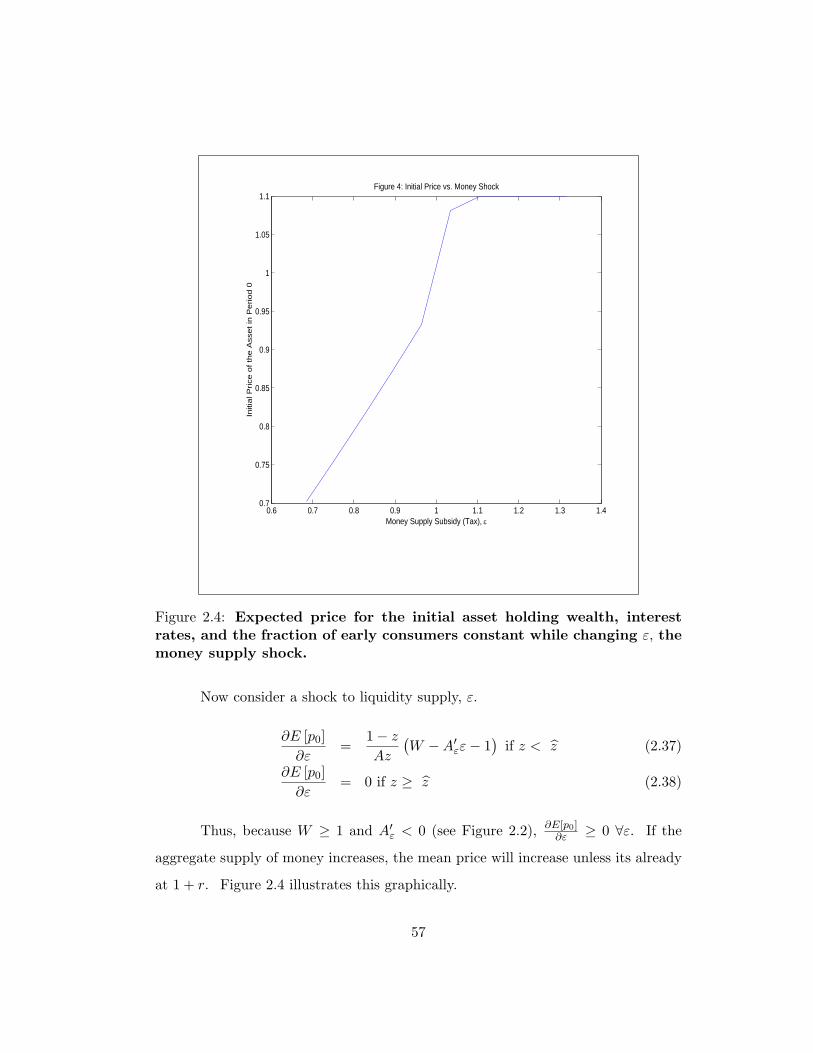
0.6 0.7 0.8 0.9 1 1.1 1.2 1.3 1.40.7

0.75

0.8

0.85

0.9

0.95

1

1.05

1.1

Money Supply Subsidy (Tax), ε

Initi

al P

rice

of th

e A

sset

in P

erio

d 0

Figure 4: Initial Price vs. Money Shock

Figure 2.4: Expected price for the initial asset holding wealth, interestrates, and the fraction of early consumers constant while changing ε, themoney supply shock.

Now consider a shock to liquidity supply, ε.

∂E [p0]∂ε

=1− z

Az

(W −A′

εε− 1)

if z < z (2.37)

∂E [p0]∂ε

= 0 if z ≥ z (2.38)

Thus, because W ≥ 1 and A′ε < 0 (see Figure 2.2), ∂E[p0]

∂ε ≥ 0 ∀ε. If the

aggregate supply of money increases, the mean price will increase unless its already

at 1 + r. Figure 2.4 illustrates this graphically.

57

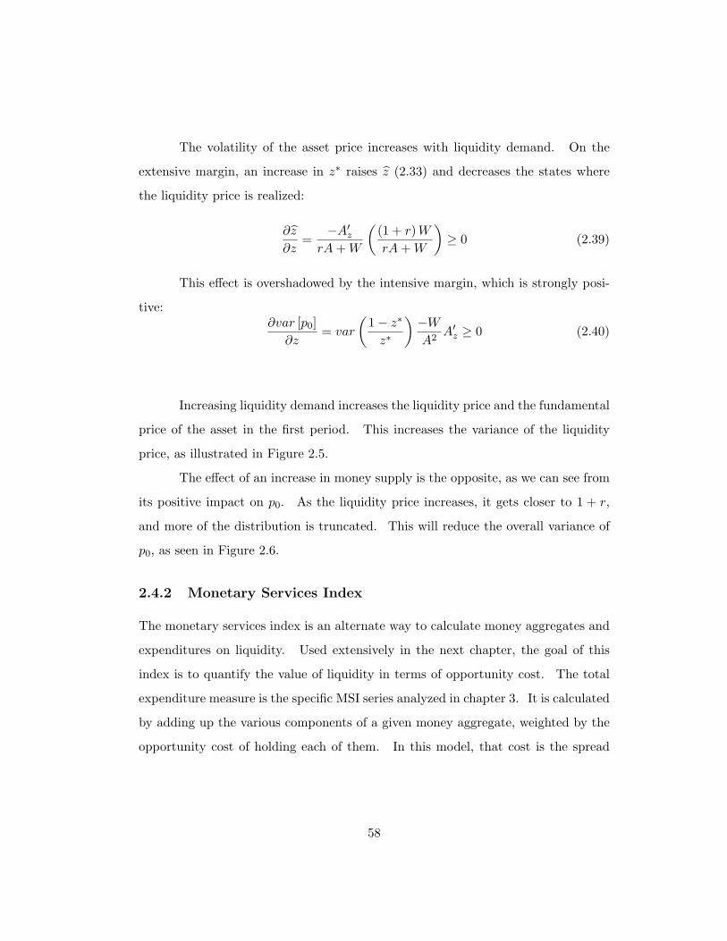
The volatility of the asset price increases with liquidity demand. On the

extensive margin, an increase in z∗ raises z (2.33) and decreases the states where

the liquidity price is realized:

∂z

∂z=

−A′z

rA+W

((1 + r)WrA+W

)≥ 0 (2.39)

This effect is overshadowed by the intensive margin, which is strongly posi-

tive:∂var [p0]

∂z= var

(1− z∗

z∗

)−WA2

A′z ≥ 0 (2.40)

Increasing liquidity demand increases the liquidity price and the fundamental

price of the asset in the first period. This increases the variance of the liquidity

price, as illustrated in Figure 2.5.

The effect of an increase in money supply is the opposite, as we can see from

its positive impact on p0. As the liquidity price increases, it gets closer to 1 + r,

and more of the distribution is truncated. This will reduce the overall variance of

p0, as seen in Figure 2.6.

2.4.2 Monetary Services Index

The monetary services index is an alternate way to calculate money aggregates and

expenditures on liquidity. Used extensively in the next chapter, the goal of this

index is to quantify the value of liquidity in terms of opportunity cost. The total

expenditure measure is the specific MSI series analyzed in chapter 3. It is calculated

by adding up the various components of a given money aggregate, weighted by the

opportunity cost of holding each of them. In this model, that cost is the spread

58

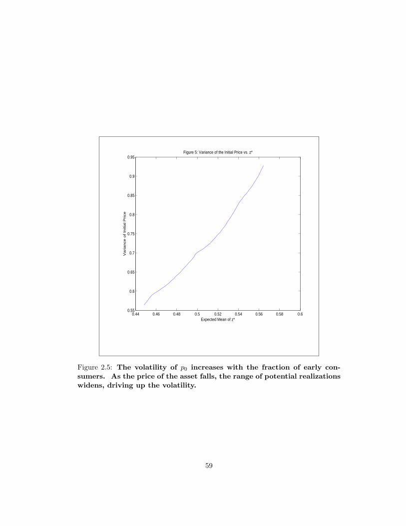
0.44 0.46 0.48 0.5 0.52 0.54 0.56 0.58 0.60.55

0.6

0.65

0.7

0.75

0.8

0.85

0.9

0.95

Expected Mean of z*

Var

ianc

e of

Initi

al P

rice

Figure 5: Variance of the Initial Price vs. z*

Figure 2.5: The volatility of p0 increases with the fraction of early con-sumers. As the price of the asset falls, the range of potential realizationswidens, driving up the volatility.

59

0.6 0.7 0.8 0.9 1 1.1 1.2 1.3 1.40

0.1

0.2

0.3

0.4

0.5

0.6

0.7

0.8

0.9

1

Money Supply Subsidy (Tax), ε

Var

ianc

e of

the

Initi

al P

rice

Figure 6: Variance of the Initial Price vs. Money Shock

Figure 2.6: The volatility of p0 decreases with the money supply shock. Asthe price of the asset rises, the range of potential realizations narrows,shrinking down the volatility until it converges to zero.

60

between the return on m and a:

ra − rm = 1 + r − p0 (2.41)

To express the total expenditure, I multiply this cost by aggregate money holdings

and substitute in the mean of p0 (when its less than 1 + r).

MSI : (1 + r − p0) (W −A) ε (2.42)

The MSI reacts positively to a shock to money demand:

∂MSI

∂z= − (1 + r − p0)

∂a0

∂z− (W −A)

∂p0

∂z(2.43)

As both asset demand and the price decline with respect to z, the price and

amount of money, the total expenditure on monetary assets, is increasing The MSI

increasing with a shock to money demand is consistent with a measure of illiquidity.

This is shown in Figure 2.7.

The opposite is true for an increase in money supply via a money shock:

∂MSI

∂ε=∂ (1 + r − p0)

∂εM +

∂M

∂ε(1 + r − p0) (2.44)

The quantity of money is increasing with ε, but its getting more expensive

per unit as well; p0 is falling, driving up the opportunity cost. Figure 2.8 shows

how the MSI decreases with ε.

The MSI increases with a liquidity demand shock and decreases with a liq-

uidity supply shock. Thus, it is a measure of illiquidity.

61

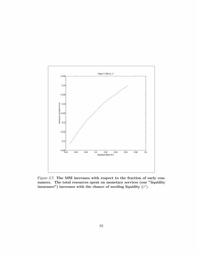
0.44 0.46 0.48 0.5 0.52 0.54 0.56 0.58 0.60.105

0.11

0.115

0.12

0.125

0.13

0.135

0.14

0.145

Expected Mean of z*

Var

ianc

e of

Initi

al P

rice

Figure 7: MSI vs. z*

Figure 2.7: The MSI increases with respect to the fraction of early con-sumers. The total resources spent on monetary services (our ”liquidityinsurance”) increases with the chance of needing liquidity (z∗).

62

0.6 0.7 0.8 0.9 1 1.1 1.2 1.3 1.40

0.02

0.04

0.06

0.08

0.1

0.12

0.14

Money Supply Subsidy (Tax), ε

Var

ianc

e of

the

Initi

al P

rice

Figure 8: MSI vs. Money Shock

Figure 2.8: The MSI decreases with respect to the money supply shock.The total resources spent on monetary services decreases as the oppor-tunity cost of holding money falls.

63

2.5 Conclusion

This paper introduces a simple asset allocation model to explore the impact of a

change in liquidity demand and supply on the price level and volatility of an asset.

I find that an increase in money supply or a decrease in liquidity demand raises the

price of the asset. Additionally, I find that volatility decreases as the liquidity price

of the asset increases. The decrease in volatility is driven by the increasingly severe

upper bound on the liquidity price, the fundamental value price. This asymmetry is

based on the idea that those with liquid assets but no immediate needs will not part

with them unless they will earn a better return, while those with illiquid assets and

immediate needs have no lower bound on what they’ll accept for their illiquid goods.

The model abstracts from transaction costs, participation costs, or other frictions,

and focuses on the interaction between the most critical component of liquidity, the

cost of converting wealth into consumption.

In preparation for the next chapter, I investigated some of the theoretical

properties of a monetary services index within the context for the model and show

that it is a measure of illiquidity. As an extension to this paper, introducing a

second type of agent, an infinitely lived market maker, may reduce the liquidity

premium but amplify the impact of a shock.

64

Chapter 3

Monetary Liquidity and Asset

Pricing

3.1 Introduction

In an effort to solve numerous finance puzzles such as excess volatility and the

equity risk premium, much attention has been directed at relaxing the assumption

of costless exchange in asset markets. Liquidity factors, as they have come to be

called, are now commonly cited indicators of the state of the market and contribute

significantly to explaining returns and volatility. While widely discussed, liquidity

can be a nebulous concept, and has been applied to areas ranging from explaining

the behavior of intraday volume of a particular stock to assessing global monetary

conditions.

In this chapter, I propose monetary liquidity as the best and most fundamen-

tal measure of the underlying distortion that liquidity factors are trying to capture.

Using a GARCH-in-mean estimation model, I show that monetary factors more

accurately match existing stylized facts of liquidity and asset returns than market

based measures of liquidity. Moreover, while this result is focused on returns and

65

volatility of an equity index over time, it is robust to cross-sectional analysis at an

individual stock level such as the decile return methodology used by Pastor and

Stambaugh (2003).

Monetary liquidity measures the cost of converting capital to consumption.

When the quantity of money is high, the cost of liquidity is low, and the difference

between selling an asset today and the value of holding it forever is very small.

Similarly, in an asset market, the cost of liquidity is interpreted as the discount in

price that a seller gives up to hold cash instead of the asset.

To the extent liquidity costs are non-zero, their will be a liquidity premium

on every transaction. This could accrue to the buyer or the seller, depending on

whose needs are greater. The seller may need to convert the asset to cash in order

to consume, the buyer may have too much cash earning a low return. Thus, the

observed transaction price is the true value of the asset plus or minus the liquidity

premium. When liquidity is high, the prices observed will be in a tight range around

true value. When liquidity is low, that range will widen out. If the distribution of

observed prices widens out about the true value, we would expect to observe higher

price volatility in periods of low liquidity. Chapter 2 of this dissertation offers a

two-period model to illustrate this mechanism.

Empirical studies linking monetary conditions, market liquidity, and asset

prices have found several common observations across different measures of market

liquidity.

F1. Illiquidity is associated with lower contemporaneous returns and higher

expected returns.

F2. Assets that are on average more illiquid have higher expected returns

than assets that are more liquid.

F3. Illiquidity is associated with higher contemporaneous price volatility.

The first two stylized facts address the link between equity returns and liq-

66

uidity. Empirical evidence for these two facts has been found using a broad array of

market liquidity measures. Amihud (2002) found that excess returns vary positively

with illiquidity, both cross-sectionally and over time. He employs an information

flow based measure of liquidity, defined as the magnitude of the change in price over

the total dollar volume. Pastor and Stambaugh (2003) found strong evidence for F2

using a liquidity measure based on order flow, which is essentially volume but only

counts the trades that change the direction of the price. They construct an order

flow index at daily frequency for most stocks on major US exchanges. In order to

find aggregate market liquidity, they average individual stock liquidity over a month

and across all stocks.

Empirical studies relating liquidity and volatility have found evidence of F3,

and most have used a GARCH based estimation methodology. Lammoureux and

Lastrapes (1990) used a GARCH model and volume based liquidity measure to test

the impact of liquidity on stock volatility. By comparing a GARCH estimation

conditioned on past volatility to a GARCH estimation conditioned on volume, they

concluded that much of the change in volatility can be attributed to the amount of

volume traded.

Chordia and Subrahmanyam (2005) is one of the few papers that considers

the role of monetary liquidity in asset markets. Using a VAR approach to jointly

estimate stock and bond liquidity, volatility, and returns, they find that monetary

policy only affects markets in extreme ”crisis periods”. The authors use a pro-

portional spread measure of liquidity, the difference in the bid/ask spread over the

average price.

Watanabe and Watanabe (Forthcoming) closely followed Lammoureux and

Lastrapes’s methodology and tested other market based measures of liquidity such as

Amihud’s price impact, Chordia’s proportional spread, and Pastor and Stambaugh’s

order flow based aggregate liquidity. They find strong support for stylized F3 for

67

all liquidity measures.

Previous finance literature has focused almost exclusively on market mea-

sures of liquidity. While these measures are excellent measures of the cost of

buying or selling an asset, they do not encompass the complete range of impacts

that the cost of liquidity can have on asset prices. Low market liquidity may oc-

cur in periods of high price volatility, and may also be a contributing factor, but

because both observations are the result of decisions made by price-taking agents,

a more fundamental process must be the source of the distortion. I am proposing

that monetary liquidity is that deeper process for two reasons. First, money is an

excellent numeraire good. It is the most common link between the asset and goods

market, and as such the cost of holding money has been argued to be a summary

statistic for economy wide liquidity costs1

In section 2, I describe the Monetary Services Index (MSI), a monetary

aggregate designed to capture the service flow provided by the money supply. This

index is designed to capture the expense of holding money, and as such is ideally

suited to measure the state of monetary liquidity in the economy.

Section 3 tests the MSI against the other, more traditional market based

liquidity measures in a GARCH-in-mean framework outlined in Lamoureux and

Lastrapes. This technique has the advantage of testing stylized facts F1 and F3

at the same time. I find that the MSI is the only measure that matches both

simultaneously.

As a further robustness check, Section 4 presents a test of the MSI using

Pastor and Stambaugh’s methodology for individual stocks. Using a test period of

5 years, I measure each stock’s sensitivity to liquidity (a liquidity ”beta”) and sort

stocks into portfolios based on their liquidity beta decile. In this method, the most1For a good survey of the literature on money aggregates as a summary of interest rates, see

Nelson (2002) and Nelson (2003). Second, disturbances in money supply are initiated by the centralbank, and are therefore not subject to stabilizing market forces and do not have to be in equilibrium.

68

important statistic is the excess return from a portfolio constructed from being long

decile 10 and short decile 1. I find that the 10-1 portfolio for the MSI is comparable

in magnitude to the 10-1 portfolio for Pastor and Stambaugh, despite their liquidity

measure being based on market data. Additionally, the market liquidity measure

doesn’t earn any excess return after controlling for monetary liquidity.

Section 5 addresses the question of which liquidity measure is more funda-

mental, and causing the other. Similar to Chordia, Sarkara and Subrahmanyam, I

estimate a VAR on returns, volatility, and both liquidity measures. Contrary to

their results, I find that monetary liquidity is the only liquidity factor that explains

return volatility, and that while there appears to be minor feedback loop through

market liquidity, monetary liquidity provides the bulk of the fundamental shock.

Section 6 concludes.

3.2 Data

Data for the liquidity metrics and returns came from several sources. For the time

series estimates of market returns and liquidity I used the monthly total return

(including dividends) index published by Standard and Poors. To calculate Ami-

hud’s measure of price impact, I took the change in the price of the index divided

by the dollar volume of shares traded. For the cross-sectional analysis, I obtained

monthly data on individual securities from CRSP. This included both total returns

and variables used to calculate market liquidity. Chordia’s measure of proportional

spread was calculated for each stock as the difference in the Ask and Bid price di-

vided by last month’s price. These values were then aggregated across stocks to

generate a value-weighted index level for stocks that are in the S&P 500. Pastor

and Stambaugh’s aggregate order flow index and liquidity innovation is available for

download through WRDS. Their index is constructed using a three step, bottom up

procedure. At the stock level, the author’s run a regression on daily stock returns

69

over a the period of a month:

ri,d+1,t = θi,t + φi,tri,d,t + γi,tsign(rei,d,t

)· vi,d,t + εi,d+1,t (3.1)

ri,d,t = ri,d,t − rm,d,t (Excess return over the market)

vi,d,t = dollar volume

The coefficient γi,t is designed to capture the ”order flow” effect. That is,

the volume of shares traded in excess of the market move for a given day should be

partially reversed if a stock is not perfectly liquid. The next step is to aggregate

γi,t, across stocks to generate an market wide measure:

γt =1N

N∑i=1

γi,t (3.2)

An AR(1) process is then parameterized to first difference of this series in

order to generate what the authors term a ”liquidity innovation”, µt :

∆γt = a+ b∆γt−1 + c

(mt−1

mt

)γt−1 + µt (3.3)

The residual of the above process, µt, is the liquidity factor used throughout

their paper and in the following comparisons.

For empirical proxies of monetary liquidity, I downloaded the Monetary Ser-

vices Index and associated indices from the St. Louis Federal Reserve. Also called

a Divisia or Fisher aggregate, these indices are constructed to weight each compo-

nent of the money aggregate by the ”moneyness” characteristics it possesses. For

example, currency is 100% money, as it generates no return and is perfectly liquid.

An interest bearing checking account is close to money, as it is a demand deposit,

but not 100%. A CD or treasury bill would only be a little like money, as it has a

fixed term. Traditional money aggregates tend to be swamped by their most illiquid

70

components, as the illiquid components carry a notional value that is much higher

than the more liquid components. I am using the MZM (money, zero maturity)

aggregate, which contains all the zero duration components of M1 and M2. I also

include the simple sum MZM aggregate to compare with the services index.

The Divisia aggregation technique creates several indices from the aggregate

components. I choose to use the total expenditure on monetary assets (referred

to henceforth as the MSI) both because it’s constructed in a more transparent way

than some of the others and it accounts for both changes in the cost of liquidity and

the quantity. The MSI computes the total expenditure of monetary assets as the

sum across all MZM components of the opportunity cost of holding the component

times the amount held (3.4).

Total Expenditure on Monetary Assets: yt =n∑i

πrealit mnom

it (3.4)

The total expenditure is measured in nominal terms, and because it is a

measure of the total economy-wide cost of liquidity services, it should be interpreted

as a measure of market illiquidity. In the following analysis, the total expenditure

on monetary assets is divided by nominal GDP to scale it across time.2

To get a sense of how the different measure of liquidity relate to one another,

and to returns, a correlation matrix is shown in Figure 3.1

The two metrics that will be the focus of this paper, Pastor and Stambaugh’s

market liquidity measure and total expenditure measure of monetary liquidity, have

almost no correlation. The low correlation between total expenditure and the

simple sum aggregation of the same MZM components highlights the impact of

the aggregation technique on the liquidity measure. The high correlation of price2For a complete description of the Monetary Services Index and its contructions, see Anderson,

Jones and Nesmith (1997). Constructing the Index has been an ongoing project at the St. LouisFederal Reserve.

71

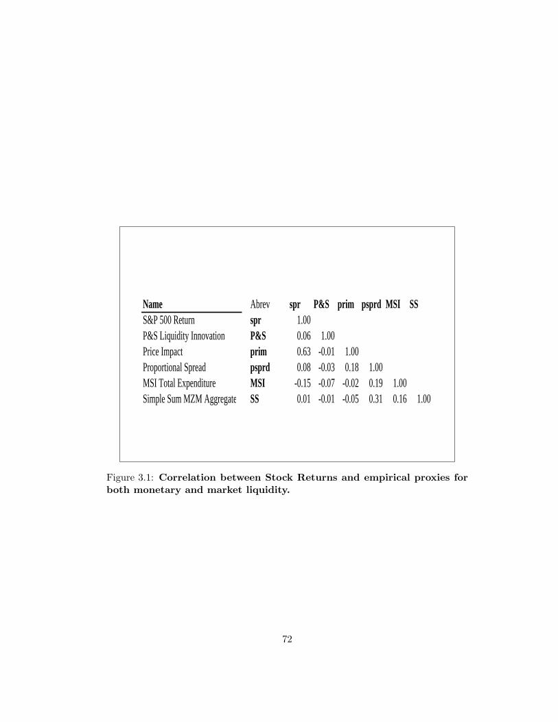
Name Abrev spr P&S prim psprd MSI SSS&P 500 Return spr 1.00P&S Liquidity Innovation P&S 0.06 1.00Price Impact prim 0.63 -0.01 1.00Proportional Spread psprd 0.08 -0.03 0.18 1.00MSI Total Expenditure MSI -0.15 -0.07 -0.02 0.19 1.00Simple Sum MZM Aggregate SS 0.01 -0.01 -0.05 0.31 0.16 1.00

Figure 3.1: Correlation between Stock Returns and empirical proxies forboth monetary and market liquidity.

72

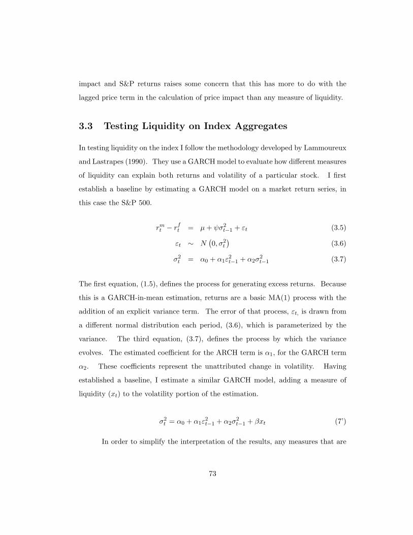
impact and S&P returns raises some concern that this has more to do with the

lagged price term in the calculation of price impact than any measure of liquidity.

3.3 Testing Liquidity on Index Aggregates

In testing liquidity on the index I follow the methodology developed by Lammoureux

and Lastrapes (1990). They use a GARCH model to evaluate how different measures

of liquidity can explain both returns and volatility of a particular stock. I first

establish a baseline by estimating a GARCH model on a market return series, in

this case the S&P 500.

rmt − rf

t = µ+ ψσ2t−1 + εt (3.5)

εt ∼ N(0, σ2

t

)(3.6)

σ2t = α0 + α1ε

2t−1 + α2σ

2t−1 (3.7)

The first equation, (1.5), defines the process for generating excess returns. Because

this is a GARCH-in-mean estimation, returns are a basic MA(1) process with the

addition of an explicit variance term. The error of that process, εt, is drawn from

a different normal distribution each period, (3.6), which is parameterized by the

variance. The third equation, (3.7), defines the process by which the variance

evolves. The estimated coefficient for the ARCH term is α1, for the GARCH term

α2. These coefficients represent the unattributed change in volatility. Having

established a baseline, I estimate a similar GARCH model, adding a measure of

liquidity (xt) to the volatility portion of the estimation.

σ2t = α0 + α1ε

2t−1 + α2σ

2t−1 + βxt (7’)

In order to simplify the interpretation of the results, any measures that are

73

conceptually measures of illiquidity (Pastor and Stambaugh’s order flow, the MSI,

and the proportional spread) I multiply by −1 to put everything in terms of a

liquidity measure.

Comparing the α1 and α2 terms in both estimations reveals the contribu-

tion of the liquidity term to explaining the volatility. This comparison is seen in

Figure 3.2. Column II is the baseline GARCH-in-mean test, columns III-V are the

GARCH-in-mean with market based liquidity measures, VI and VII are monetary

based liquidity measures. In order to determine whether the liquidity factors con-

tribute to explaining volatility compare the size and significance of α1 and α2 in the

baseline case to the cases with a liquidity factor. The ARCH term, α1, is much

reduced in both size and statistical significant by the each of the market liquidity

factors.3 The monetary factors had no impact on the ARCH term.

The GARCH term, α2, reveals more of an impact. Models IV-VI, price

impact, proportional spread, and the Monetary Services Index, reduce α2 to the

point of being statistically insignificant. Model II, Pastor and Stambaugh’s order

flow measure, as well as model VII, the simple sum money aggregate, fail to explain

any of the GARCH term.

Having established that the monetary services index is statistically significant

in explaining volatility, I can use the results of the estimation to evaluate each model

on how closely it matches the two time-series based stylized facts (F1 and F3).

To test stylized F1, we need to determine the impact of liquidity on the

excess return. In the estimation model, this is calculated by multiplying ψ, the

GARCH-in-mean coefficient, by βn, the coefficient of liquidity in the expression for

variance. The product of these two coefficients is seen in the last row of Figure

3.2. In order to confirm F1, ψβn needs to be positive, as these are all measures of

liquidity. Of the market liquidity measures, only Amihud’s measure of proportional3This is a similar result to Watanabe and Watanabe (Forthcoming).

74

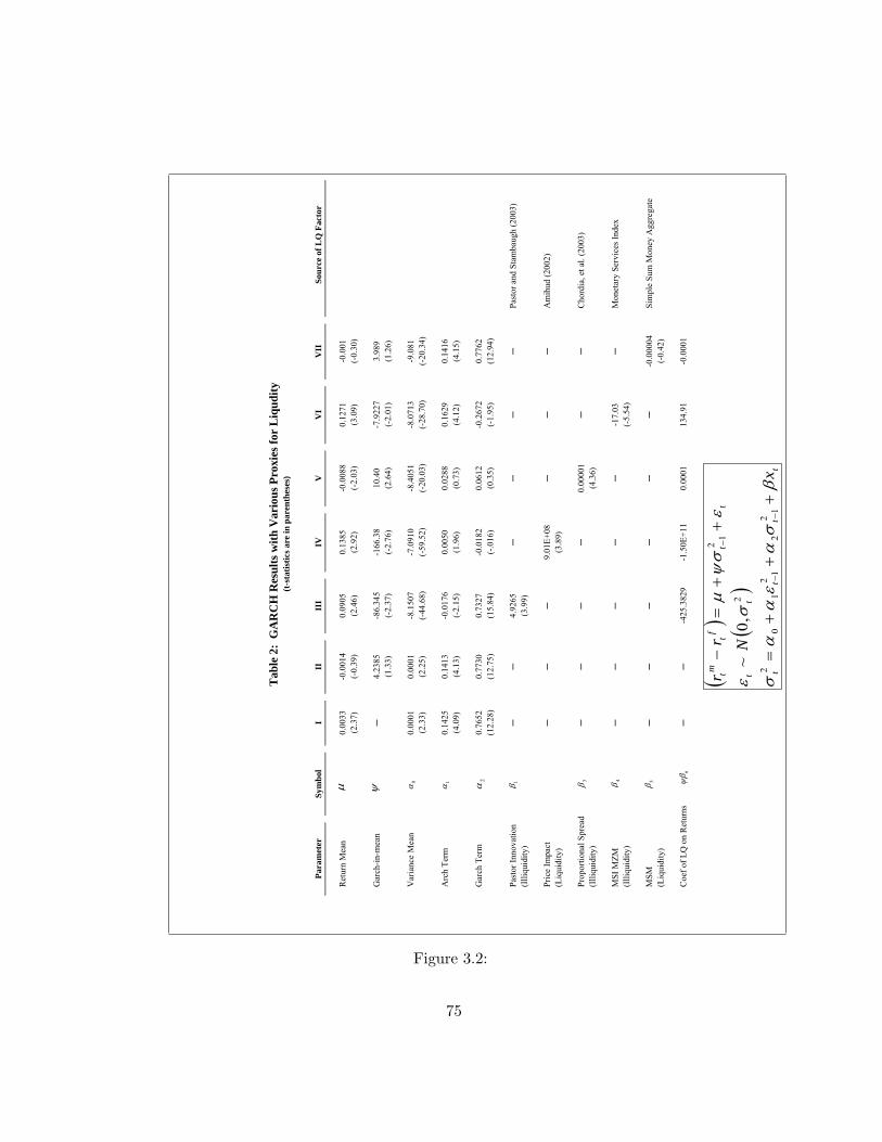
Tab

le 2

: G

AR

CH

Res

ults

with

Var

ious

Pro

xies

for

Liq

udity

(t-s

tatis

tics a

re in

par

enth

eses

)

Para

met

erSy

mbo

lI

IIII

IIV

VV

IV

IISo

urce

of L

Q F

acto

r

Ret

urn

Mea

n0.

0033

-0.0

014

0.09

050.

1385

-0.0

088

0.12

71-0

.001

(2.3

7)(-

0.39

)(2

.46)

(2.9

2)(-

2.03

)(3

.09)

(-0.

30)

Gar

ch-in

-mea

n─

4.23

85-8

6.34

5-1

66.3

810

.40

-7.9

227

3.98

9(1

.33)

(-2.

37)

(-2.

76)

(2.6

4)(-

2.01

)(1

.26)

Var

ianc

e M

ean

0.00

010.

0001

-8.1

507

-7.0

910

-8.4

051

-8.0

713

-9.0

81(2

.33)

(2.2

5)(-

44.6

8)(-

59.5

2)(-

20.0

3)(-

28.7

0)(-

20.3

4)

Arc

h Te

rm0.

1425

0.14

13-0

.017

60.

0050

0.02

880.

1629

0.14

16(4

.09)

(4.1

3)(-

2.15

)(1

.96)

(0.7

3)(4

.12)

(4.1

5)

Gar

ch T

erm

0.76

520.

7730

0.73

27-0

.018

20.

0612

-0.2

672

0.77

62(1

2.28

)(1

2.75

)(1

5.84

)(-

.016

)(0

.35)

(-1.

95)

(12.

94)

Past

or In

nova

tion

──

4.92

65─

──

─Pa

stor

and

Sta

mba

ugh

(200

3)(I

lliqu

idity

)(3

.99)

Pric

e Im

pact

──

─9.

01E+

08─

──

Am

ihud

(200

2)(L

iqui

dity

)(3

.89)

Prop

ortio

nal S

prea

d─

──

─0.

0000

1─

─C

hord

ia, e

t al.

(200

3)(I

lliqu

idity

)(4

.36)

MSI

MZM

──

──

─-1

7.03

─M

onet

ary

Serv

ices

Inde

x(I

lliqu

idity

)(-

5.54

)

MSM

──

──

──

-0.0

0004

Sim

ple

Sum

Mon

ey A

ggre

gate

(Liq

uidi

ty)

(-0.

42)

Coe

f of L

Q o

n R

etur

ns─

─-4

25.3

829

-1.5

0E+1

10.

0001

134.

91-0

.000

1

0α

1α

2α 1β

2β 3β 4β 5βµ ψ

() (

)t

tt

t

tt

tt

f tm t

x

Nrr

βσ

αε

αα

σ

σε

εψσ

µ

++

+=

++

=−

−−

−

21

22

11

02

2

21

,0~

nψβ

Figure 3.2:

75

spread delivers this result. Of the monetary liquidity measures, the Monetary

Services index matches F1 but the simple sum aggregate does not.

To test F3, that volatility increases in illiquid environments, we need only to

determine the βn coefficient. For measures of liquidity, a negative βn would confirm

F3. On this basis, none of the market measures of liquidity match. βn for models

III, IV, and V, (order flow, price impact, and proportional spread), is significant but

negative. The result suggests volatility is higher in liquid environments, contrary

to F3. The monetary models do better: the MSI is both negative and significant.

The simple sum aggregate is negative, which is consistent with liquidity reducing

volatility, though it’s not significant.

The GARCH estimation produces two results. First, that monetary mea-

sures of liquidity contribute to explaining return volatility beyond that of market

liquidity. We infer this from the reduced size and significance of the generalized

ARCH and GARCH terms, α1, and α2. Secondly, that monetary liquidity is seen to

reduce volatility and increase returns simultaneously. None of the market liquidity

measures were observed doing both at once.

3.4 Testing Liquidity on a Cross-Section of Stocks

The previous section established that monetary liquidity preforms as well or better

than market liquidity in matching the stylized facts of returns and volatility at

an aggregate level and over time. In order to show this result to be robust, the

monetary measures should explain a liquidity based excess return over a cross-section

of stocks, thereby matching F2. A major strength of Pastor and Stambaugh (2003)

is their result that excess returns can be attributed to a particular stock’s sensitivity

to the aggregate liquidity factor. They show this using the decile ranking approach

pioneered by Fama and Macbeth (1973). In order to evaluate how well monetary

factors match F2, I replicate Pastor and Stambaugh’s procedure of checking decile

76

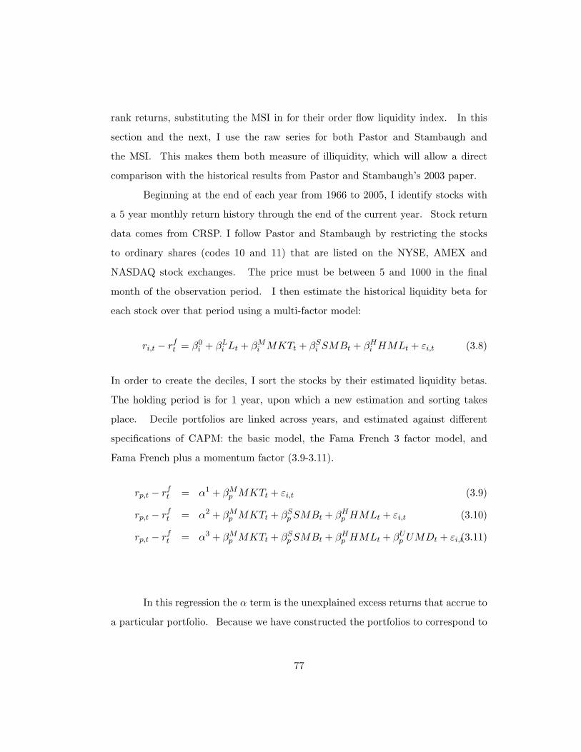
rank returns, substituting the MSI in for their order flow liquidity index. In this

section and the next, I use the raw series for both Pastor and Stambaugh and

the MSI. This makes them both measure of illiquidity, which will allow a direct

comparison with the historical results from Pastor and Stambaugh’s 2003 paper.

Beginning at the end of each year from 1966 to 2005, I identify stocks with

a 5 year monthly return history through the end of the current year. Stock return

data comes from CRSP. I follow Pastor and Stambaugh by restricting the stocks

to ordinary shares (codes 10 and 11) that are listed on the NYSE, AMEX and

NASDAQ stock exchanges. The price must be between 5 and 1000 in the final

month of the observation period. I then estimate the historical liquidity beta for

each stock over that period using a multi-factor model:

ri,t − rft = β0

i + βLi Lt + βM

i MKTt + βSi SMBt + βH

i HMLt + εi,t (3.8)

In order to create the deciles, I sort the stocks by their estimated liquidity betas.

The holding period is for 1 year, upon which a new estimation and sorting takes

place. Decile portfolios are linked across years, and estimated against different

specifications of CAPM: the basic model, the Fama French 3 factor model, and

Fama French plus a momentum factor (3.9-3.11).

rp,t − rft = α1 + βM

p MKTt + εi,t (3.9)

rp,t − rft = α2 + βM

p MKTt + βSp SMBt + βH

p HMLt + εi,t (3.10)

rp,t − rft = α3 + βM

p MKTt + βSp SMBt + βH

p HMLt + βUp UMDt + εi,t(3.11)

In this regression the α term is the unexplained excess returns that accrue to

a particular portfolio. Because we have constructed the portfolios to correspond to

77

a particular decile ranking of liquidity sensitivity, comparing the alphas reveals any

returns to liquidity exposure. By slowly increasing the number of dependent vari-

ables, other potential risk factors that may be correlated with liquidity are filtered

out. For example, larger firms tend to be more liquid, so putting just the market

return on the right hand side wouldn’t rule out the impact from size. In their

paper, Pastor and Stambaugh preformed this analysis with stocks equal weighted

and value weighted. The results were not significantly affected. All results shown

here are value-weighted.

Figure 3.3 shows the alphas (or unexplained excess returns) that result from

estimating each decile portfolio on different versions of a CAPM model (3.9-3.11).

The most important column in these tables is the results for the 10-1 portfolio, as it

arguably cancels out unexplained noise, and allows for the most precise estimation

of the alpha associated with a particular model. The 10-1 alphas are attempting

to capture exposure to the liquidity factor without any other factor returns mixed

in. None of the alphas at the four factor (3.11) level were significant for the MSI.

Compare these results with the Figure 3.4, which shows the results from an identical

procedure using the Pastor and Stambaugh measure of liquidity (Table 8 in their

paper). The 10-1 level alpha’s were positive and statistically significant for even

the four risk factor model.

One surprising result from this analysis is that the excess return on the MSI

10-1 alphas are negative. Investors usually demand a higher return to take on more

exposure to a risk factor. It’s possible that because the MSI is an economy wide

measure, it’s correlated with investors fluctuating demand as well. If liquidity costs

rise with sudden changes in wealth, it may be more desirable to own a stock that

goes up at the same time an agent would like to sell it. This would reduce the risk

premium on decile 10 stocks and increase in for decile 1 stocks.

The decile ranking analysis of the MSI factor yielded interesting results, but

78

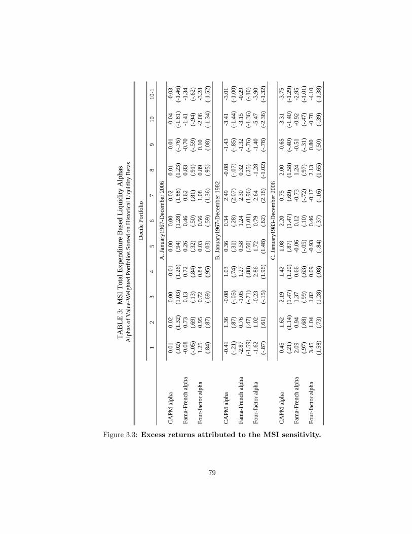
TAB

LE 3

: M

SI T

otal

Exp

endi

ture

Bas

ed L

iqui

dity

Alp

has

Alp

has o

f Val

ue-W

eigh

ted

Portf

olio

s Sor

ted

on H

isto

rical

Liq

uidi

ty B

etas

Dec

ile P

ortfo

lio

12

34

56

78

910

10-1

A. J

anua

ry19

67-D

ecem

ber 2

006

CA

PM a

lpha

0.01

0.02

0.00

-0.0

10.

000.

000.

020.

01-0

.01

-0.0

4-0

.03

(.02)

(1.3

2)(1

.03)

(1.2

6)(.9

4)(1

.28)

(1.8

8)(1

.23)

(-.7

6)(-

1.81

)(-

1.46

)Fa

ma-

Fren

ch a

lpha

-0.0

80.

730.

130.

720.

260.

460.

620.

83-0

.70

-1.4

1-1

.34

(-.0

5)(.6

9)(.1

3)(.8

4)(.3

2)(.5

0)(.8

1)(.9

1)(-

.59)

(-.9

4)(-

.62)

Four

-fac

tor a

lpha

1.25

0.95

0.72

0.84

0.03

0.56

1.08

0.89

0.10

-2.0

6-3

.28

(.84)

(.87)

(.69)

(.95)

(.03)

(.59)

(1.3

6)(.9

5)(.0

8)(-

1.34

)(-

1.52

)B

. Jan

uary

1967

-Dec

embe

r 198

2C

APM

alp

ha-0

.41

1.36

-0.0

81.

030.

360.

342.

49-0

.08

-1.4

3-3

.41

-3.0

1(-

.21)

(.87)

(-.0

5)(.7

4)(.3

1)(.2

8)(2

.07)

(-.0

7)(-

.85)

(-1.

44)

(-1.

00)

Fam

a-Fr

ench

alp

ha-2

.87

0.76

-1.0

51.

270.

581.

242.

300.

32-1

.32

-3.1

5-0

.29

(-1.

59)

(.47)

(-.7

1)(.8

8)(.5

0)(1

.01)

(1.9

6)(.2

5)(-

.76)

(-1.

36)

(-.1

0)Fo

ur-f

acto

r alp

ha-1

.62

1.02

-0.2

32.

861.

720.

792.

64-1

.28

-1.4

0-5

.47

-3.9

0(-

.87)

(.61)

(-.1

5)(1

.96)

(1.4

8)(.6

2)(2

.16)

(-1.

02)

(-.7

8)(-

2.36

)(-

1.32

)

C. J

anua

ry19

83-D

ecem

ber 2

006

CA

PM a

lpha

0.45

1.62

2.19

1.42

1.08

2.20

0.75

2.00

-0.6

5-3

.31

-3.7

5(.2

1)(1

.14)

(1.4

7)(1

.20)

(.87)

(1.4

7)(.6

9)(1

.58)

(-.4

0)(-

1.40

)(-

1.29

)Fa

ma-

Fren

ch a

lpha

2.09

0.94

1.37

0.66

-0.0

60.

12-0

.73

1.24

-0.5

1-0

.92

-2.9

5(.9

7)(.6

8)(.9

9)(.6

3)(-

.05)

(.10)

(-.7

2)(.9

7)(-

.31)

(-.4

7)(-

1.01

)Fo

ur-f

acto

r alp

ha3.

451.

041.

820.

09-0

.93

0.46

-0.1

72.

130.

80-0

.78

-4.1

0(1

.58)

(.73)

(1.2

8)(.0

8)(-

.84)

(.37)

(-.1

6)(1

.65)

(.50)

(-.3

9)(-

1.38

)

Figure 3.3: Excess returns attributed to the MSI sensitivity.

79

TAB

LE 4

: Pa

stor

and

Sta

mba

ugh

Ord

er F

low

Bas

ed L

iqui

dity

Alp

has

Alp

has o

f Val

ue-W

eigh

ted

Portf

olio

s Sor

ted

on H

isto

rical

Liq

uidi

ty B

etas

Dec

ile P

ortfo

lio

12

34

56

78

910

10-1

A. J

anua

ry19

67-D

ecem

ber 2

006

CA

PM a

lpha

-2.8

3-0

.76

0.06

0.65

0.16

1.70

1.69

0.98

0.85

2.74

5.71

(-1.

93)

(-.7

1)(.0

6)(.7

4)(.1

9)(2

.00)

(1.9

0)(1

.05)

(.87)

(2.2

0)(2

.95)

Fam

a-Fr

ench

alp

ha-1

.49

-1.1

1-0

.05

0.29

-0.3

80.

870.

480.

070.

442.

984.

54(-

1.07

)(-

1.02

)(-

.05)

(.36)

(-.4

7)(1

.12)

(.57)

(.08)

(.45)

(2.3

8)(2

.32)

Four

-fac

tor a

lpha

-2.2

2-1

.62

-0.8

10.

210.

790.

680.

550.

841.

553.

515.

85(-

1.57

)(-

1.47

)(-

.87)

(.26)

(.97)

(.86)

(.64)

(.89)

(1.5

6)(2

.73)

(2.9

2)

B. J

anua

ry19

67-D

ecem

ber 1

982

CA

PM a

lpha

-0.8

10.

231.

22-0

.23

0.41

-0.1

30.

90-0

.32

-0.6

53.

063.

90(-

.34)

(.16)

(1.0

2)(-

.19)

(.36)

(-.1

0)(.8

1)(-

.23)

(-.4

7)(1

.76)

(1.4

1)Fa

ma-

Fren

ch a

lpha

-0.5

61.

312.

120.

460.

05-0

.66

0.38

-1.4

2-1

.02

2.04

2.61

(-.2

4)(.8

8)(1

.84)

(.39)

(.05)

(-.5

2)(.3

5)(-

1.01

)(-

.73)

(1.2

2)(.9

3)Fo

ur-f

acto

r alp

ha-2

.95

1.41

1.21

-0.1

11.

00-0

.24

0.56

-0.0

70.

741.

624.

70(-

1.29

)(.9

0)(1

.03)

(-.0

9)(.8

6)(-

.18)

(.49)

(-.0

5)(.5

3)(.9

3)(1

.62)

C. J

anua

ry19

83-D

ecem

ber 2

006

CA

PM a

lpha

-4.1

1-1

.01

-0.6

71.

31-0

.15

3.12

2.60

1.87

2.03

2.63

7.00

(-2.

21)

(-.6

9)(-

.47)

(1.0

5)(-

.13)

(2.8

2)(2

.02)

(1.5

1)(1

.53)

(1.5

1)(2

.61)

Fam

a-Fr

ench

alp

ha-1

.98

-2.2

2-1

.35

0.23

-0.8

92.

171.

020.

931.

523.

775.

86(-

1.13

)(-

1.55

)(-

1.01

)(.2

1)(-

.78)

(2.2

0)(.8

5)(.7

5)(1

.11)

(2.1

3)(2

.16)

Four

-fac

tor a

lpha

-2.0

8-2

.94

-2.0

50.

380.

361.

701.

111.

402.

324.

606.

81(-

1.16

)(-

2.03

)(-

1.52

)(.3

3)(.3

2)(1

.70)

(.91)

(1.1

0)(1

.68)

(2.5

5)(2

.46)

Figure 3.4: Excess returns attributed to the order flow sensitivity.

80

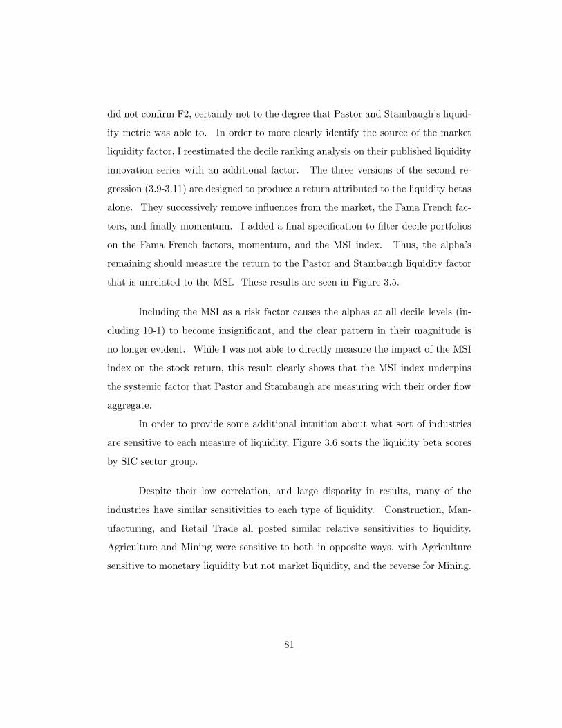
did not confirm F2, certainly not to the degree that Pastor and Stambaugh’s liquid-

ity metric was able to. In order to more clearly identify the source of the market

liquidity factor, I reestimated the decile ranking analysis on their published liquidity

innovation series with an additional factor. The three versions of the second re-

gression (3.9-3.11) are designed to produce a return attributed to the liquidity betas

alone. They successively remove influences from the market, the Fama French fac-

tors, and finally momentum. I added a final specification to filter decile portfolios

on the Fama French factors, momentum, and the MSI index. Thus, the alpha’s

remaining should measure the return to the Pastor and Stambaugh liquidity factor

that is unrelated to the MSI. These results are seen in Figure 3.5.

Including the MSI as a risk factor causes the alphas at all decile levels (in-

cluding 10-1) to become insignificant, and the clear pattern in their magnitude is

no longer evident. While I was not able to directly measure the impact of the MSI

index on the stock return, this result clearly shows that the MSI index underpins

the systemic factor that Pastor and Stambaugh are measuring with their order flow

aggregate.

In order to provide some additional intuition about what sort of industries

are sensitive to each measure of liquidity, Figure 3.6 sorts the liquidity beta scores

by SIC sector group.

Despite their low correlation, and large disparity in results, many of the

industries have similar sensitivities to each type of liquidity. Construction, Man-

ufacturing, and Retail Trade all posted similar relative sensitivities to liquidity.

Agriculture and Mining were sensitive to both in opposite ways, with Agriculture

sensitive to monetary liquidity but not market liquidity, and the reverse for Mining.

81

TAB

LE 5

: Pa

stor

and

Sta

mba

ugh

Ord

er F

low

Bas

ed L

iqui

dity

Alp

has,

Filte

red

on th

e M

SIA

lpha

s of V

alue

-Wei

ghte

d Po

rtfol

ios S

orte

d on

His

toric

al L

iqui

dity

Bet

a

Dec

ile P

ortfo

lio

12

34

56

78

910

10-1

A. J

anua

ry19

67-D

ecem

ber 2

006

CA

PM a

lph a

-2.8

3-0

.76

0.06

0.65

0.16

1.70

1.69

0.98

0.85

2.74

5.71

(-1.

93)

(-.7

1)(.0

6)(.7

4)(.1

9)(2

.00)

(1.9

0)(1

.05)

(.87)

(2.2

0)(2

.95)

Fam

a-Fr

ench

alp

ha-1

.49

-1.1

1-0

.05

0.29

-0.3

80.

870.

480.

070.

442.

984.

54(-

1.07

)(-

1.02

)(-

.05)

(.36)

(-.4

7)(1

.12)

(.57)

(.08)

(.45)

(2.3

8)(2

.32)

Four

-fac

tor a

lpha

-2.2

2-1

.62

-0.8

10.

210.

790.

680.

550.

841.

553.

515.

85(-

1.57

)(-

1.47

)(-

.87)

(.26)

(.97)

(.86)

(.64)

(.89)

(1.5

6)(2

.73)

(2.9

2)FF

4 +

MSI

Liq

uidi

ty A

lpha

4.60

2.30

-4.8

42.

095.

39-4

.00

2.79

1.80

-8.5

0-3

.56

-7.8

3(.5

9)(.3

7)(-

.99)

(.46)

(1.2

0)(-

.95)

(.59)

(.35)

(-1.

66)

(-.5

3)(-

.78)

B. J

anua

ry19

67-D

ecem

ber 1

982

CA

PM a

lpha

-0.8

10.

231.

22-0

.23

0.41

-0.1

30.

90-0

.32

-0.6

53.

063.

90(-

.34)

(.16)

(1.0

2)(-

.19)

(.36)

(-.1

0)(.8

1)(-

.23)

(-.4

7)(1

.76)

(1.4

1)Fa

ma-

Fren

ch a

lpha

-0.5

61.

312.

120.

460.

05-0

.66

0.38

-1.4

2-1

.02

2.04

2.61

(-.2

4)(.8

8)(1

.84)

(.39)

(.05)

(-.5

2)(.3

5)(-

1.01

)(-

.73)

(1.2

2)(.9

3)Fo

ur-f

acto

r alp

ha-2

.95

1.41

1.21

-0.1

11.

00-0

.24

0.56

-0.0

70.

741.

624.

70(-

1.29

)(.9

0)(1

.03)

(-.0

9)(.8

6)(-

.18)

(.49)

(-.0

5)(.5

3)(.9

3)(1

.62)

FF4

+ M

SI L

iqui

dity

Alp

ha-1

.13

1.79

-7.7

24.

438.

71-4

.01

1.01

4.51

-12.

77-9

.07

-8.0

2(-

.10)

(.22)

(-1.

35)

(.70)

(1.4

2)(-

.61)

(.17)

(.61)

(-1.

93)

(-1.

07)

(-.5

7)

C. J

anua

ry19

83-D

ecem

ber 2

006

CA

PM a

lpha

-4.1

1-1

.01

-0.6

71.

31-0

.15

3.12

2.60

1.87

2.03

2.63

7.00

(-2.

21)

(-.6

9)(-

.47)

(1.0

5)(-

.13)

(2.8

2)(2

.02)

(1.5

1)(1

.53)

(1.5

1)(2

.61)

Fam

a-Fr

ench

alp

ha-1

.98

-2.2

2-1

.35

0.23

-0.8

92.

171.

020.

931.

523.

775.

86(-

1.13

)(-

1.55

)(-

1.01

)(.2

1)(-

.78)

(2.2

0)(.8

5)(.7

5)(1

.11)

(2.1

3)(2

.16)

Four

-fac

tor a

lpha

-2.0

8-2

.94

-2.0

50.

380.

361.

701.

111.

402.

324.

606.

81(-

1.16

)(-

2.03

)(-

1.52

)(.3

3)(.3

2)(1

.70)

(.91)

(1.1

0)(1

.68)

(2.5

5)(2

.46)

FF4

+ M

SI L

iqui

dity

Alp

ha9.

8212

.26

2.61

1.96

3.72

-9.7

05.

48-4

.54

-9.2

9-6

.59

-15.

05(.8

8)(1

.31)

(.32)

(.28)

(.54)

(-1.

71)

(.72)

(-.6

0)(-

1.19

)(-

.64)

(-1.

01)

Figure 3.5: Excess returns attributed to the order flow sensitivity net ofMSI.

82

Pastor and Stambaugh Liquidity Factor Beta MSI Liquidity Factor BetaSIC

Industry MeanStandard

Dev Obs RankSIC

Industry MeanStandard

Dev Obs RankAgriculture 1 0.06 0.45 2652 2 1 -0.24 1.33 2652 9Mining 2 -0.07 0.48 41211 10 2 0.26 1.61 41211 1Construction 3 -0.04 0.51 12921 9 3 -0.33 1.54 12921 10Manufacturing 4 0.01 0.45 492675 5 4 0.13 1.53 492675 4Transportation & Utilities 5 -0.01 0.32 118102 6 5 -0.14 1.03 118102 8Wholesale Trade 6 0.02 0.46 38356 4 6 0.17 1.67 38356 3Retail Trade 7 0.03 0.45 73475 3 7 0.22 1.40 73475 2Financial Services 8 -0.03 0.35 201694 7 8 -0.10 1.11 201694 7Services 9 -0.03 0.53 97292 8 9 0.06 1.88 97292 6Public Administration 10 0.13 0.37 404 1 10 0.08 1.28 404 5

Figure 3.6: Liquidity Betas by industry group. Observations are in termsof stock-month pairs.

3.5 Causality

From the GARCH analysis we can conclude that both monetary liquidity and market

liquidity have an impact on market returns and volatility. Repeating Pastor and

Stambaugh’s decile ranking analysis shows that the two types of liquidity are related,

as accounting for one removes the effect of the other. This interrelatedness is

more complicated than a simple linear relationship, as the correlation between the

two is almost zero, and the decile ranking on monetary liquidity alone yielded no

statistically significant results. To understand the relationship between the two

types of liquidity better, it’s important to establish if changes in one are causing

changes in the other. From a conceptual perspective, it’s reasonable to believe

that monetary liquidity is the fundamental cause of market liquidity. The Federal

Reserve and the banking system are concerned with the economy as a whole, and

routinely change or distort the price and quantity of monetary instruments. Market

83

liquidity is the result of individual agents choosing to trade in a competitive market

where agents are price takers with respect to both assets and liquidity. However, it

can be argued that the Federal Reserve is influenced by market events, particularly

when market liquidity is low. In an attempt to measure the competing sources of

causation, I estimate a Vector Auto Regression of S&P 500 returns, the monthly

volatility of those returns, the Pastor and Stambaugh market liquidity innovation

and the MSI total expenditure. The monthly volatility of the S&P 500 returns is

estimated from the base GARCH case. Both liquidity measures are of illiquidity.

The results are presented in Figure 3.7.

3.5.1 Impact of Monetary vs. Market Liquidity on Returns and

Volatility

I specify a VAR with four lags based on the AIC lag selection criteria. With

both types of liquidity accounted for, the MSI is significant in explaining returns

and volatility, while the market liquidity measure in only significant in explaining

returns. Figure 3.8 shows the cumulative impulse response function for a 1% shock

to liquidity on returns. The panel on the left is the response of returns to an

innovation in market liquidity, the right to monetary liquidity. Both are significant

at the 95% level.

Figure 3.9 shows a similar impulse response function for monthly return

volatility. In the left panel, we see that market liquidity is not significant at the

95% level while on the right, monetary liquidity is.

These results are at odds with a similar analysis in Chordia and Subrah-

manyam (2005). They ran a similar VAR with fed funds as the proxy for monetary

liquidity. They found it to only be significant in ”crisis periods” of severe market

illiquidity. I attribute the difference to the broader scope of the MSI total expen-

diture series. It will pick up not only the change in fed funds, but also how the

84

Table 7: VAR(4) of Returns, Volatily, Market and Monetary Liquidity

RMSE R-sq Chi2S&P 500 Return 0.41 0.979 24343.7 Sample Period Feb-62 to Dec-05S&P 500 Volatility 3.04 0.950 9923.1 Observations 524MSI Total Exp. 0.01 0.915 5649.1P&S LQ Innovation 0.05 0.047 25.7

Coefficient Std. Error t-stat Coefficient Std. Error t-statS&P 500 Return MSI Total Expenditure

L (1) S&P 500 Ret. 1.30 0.044 29.58 L (1) S&P 500 Ret. 0.001 0.001 2.28L (2) S&P 500 Ret. -0.26 0.096 -2.73 L (2) S&P 500 Ret. -0.002 0.001 -1.33L (3) S&P 500 Ret. 0.16 0.120 1.34 L (3) S&P 500 Ret. 0.000 0.002 -0.02L (4) S&P 500 Ret. -0.20 0.073 -2.72 L (4) S&P 500 Ret. 0.000 0.001 0.39L (1) S&P 500 Vol. 0.02 0.006 3.58 L (1) S&P 500 Vol. 0.000 0.000 0.41L (2) S&P 500 Vol. 0.00 0.007 0.56 L (2) S&P 500 Vol. 0.000 0.000 -1.87L (3) S&P 500 Vol. -0.01 0.005 -1.22 L (3) S&P 500 Vol. 0.000 0.000 2.05L (4) S&P 500 Vol. -0.01 0.004 -3.49 L (4) S&P 500 Vol. 0.000 0.000 0.00L (1) MSI Tot. Exp. -27.84 3.145 -8.85 L (1) MSI Tot. Exp. 1.182 0.044 26.80L (2) MSI Tot. Exp. 28.58 4.877 5.86 L (2) MSI Tot. Exp. -0.379 0.068 -5.54L (3) MSI Tot. Exp. 1.71 5.090 0.34 L (3) MSI Tot. Exp. 0.084 0.071 1.17L (4) MSI Tot. Exp. -4.58 3.459 -1.33 L (4) MSI Tot. Exp. 0.071 0.049 1.47L (1) P&S LQ Innv. -1.16 0.387 -3.00 L (1) P&S LQ Innv. 0.011 0.005 2.04L (2) P&S LQ Innv. -0.56 0.389 -1.45 L (2) P&S LQ Innv. -0.001 0.005 -0.10L (3) P&S LQ Innv. -0.33 0.386 -0.86 L (3) P&S LQ Innv. 0.005 0.005 0.98L (4) P&S LQ Innv. 0.40 0.386 1.05 L (4) P&S LQ Innv. -0.011 0.005 -2.05Constant 0.11 0.099 1.12 Constant 0.003 0.001 2.47

S&P 500 Volatility P&S Liquidity InnovationL (1) S&P 500 Ret. -10.11 0.327 -30.89 L (1) S&P 500 Ret. 0.013 0.005 2.58L (2) S&P 500 Ret. 12.60 0.720 17.50 L (2) S&P 500 Ret. -0.015 0.011 -1.42L (3) S&P 500 Ret. -2.25 0.899 -2.50 L (3) S&P 500 Ret. 0.002 0.014 0.18L (4) S&P 500 Ret. -0.38 0.549 -0.69 L (4) S&P 500 Ret. 0.001 0.008 0.14L (1) S&P 500 Vol. 0.72 0.043 16.51 L (1) S&P 500 Vol. 0.001 0.001 0.86L (2) S&P 500 Vol. 0.35 0.052 6.78 L (2) S&P 500 Vol. 0.000 0.001 -0.02L (3) S&P 500 Vol. -0.04 0.037 -0.97 L (3) S&P 500 Vol. -0.001 0.001 -1.26L (4) S&P 500 Vol. -0.08 0.031 -2.72 L (4) S&P 500 Vol. 0.000 0.000 0.87L (1) MSI Tot. Exp. 6.04 23.486 0.26 L (1) MSI Tot. Exp. 0.238 0.357 0.67L (2) MSI Tot. Exp. 136.12 36.422 3.74 L (2) MSI Tot. Exp. -0.046 0.553 -0.08L (3) MSI Tot. Exp. -156.17 38.009 -4.11 L (3) MSI Tot. Exp. -0.644 0.577 -1.12L (4) MSI Tot. Exp. 31.96 25.830 1.24 L (4) MSI Tot. Exp. 0.180 0.392 0.46L (1) P&S LQ Innv. -2.56 2.889 -0.89 L (1) P&S LQ Innv. -0.010 0.044 -0.23L (2) P&S LQ Innv. -2.38 2.908 -0.82 L (2) P&S LQ Innv. 0.029 0.044 0.66L (3) P&S LQ Innv. 0.49 2.882 0.17 L (3) P&S LQ Innv. 0.082 0.044 1.88L (4) P&S LQ Innv. 0.35 2.879 0.12 L (4) P&S LQ Innv. -0.083 0.044 -1.90Constant -1.91 0.743 -2.57 Constant 0.026 0.011 2.31

Figure 3.7: Results of a vector autoregression including both the MSI andthe order-flow measure of liquidity

85

Figure 3.8: Cumulative response of S&P 500 returns to a 1% shock tomarket liquidity (left) and monetary liquidity (right).

86

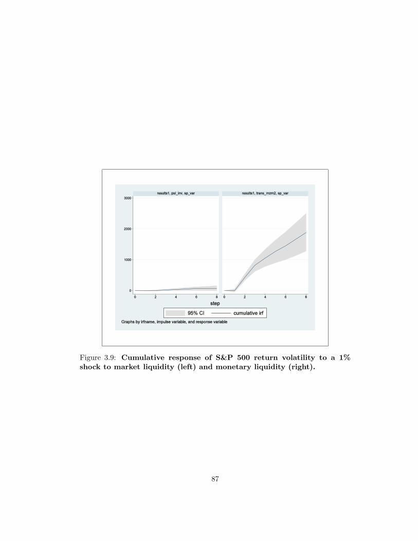
Figure 3.9: Cumulative response of S&P 500 return volatility to a 1%shock to market liquidity (left) and monetary liquidity (right).

87

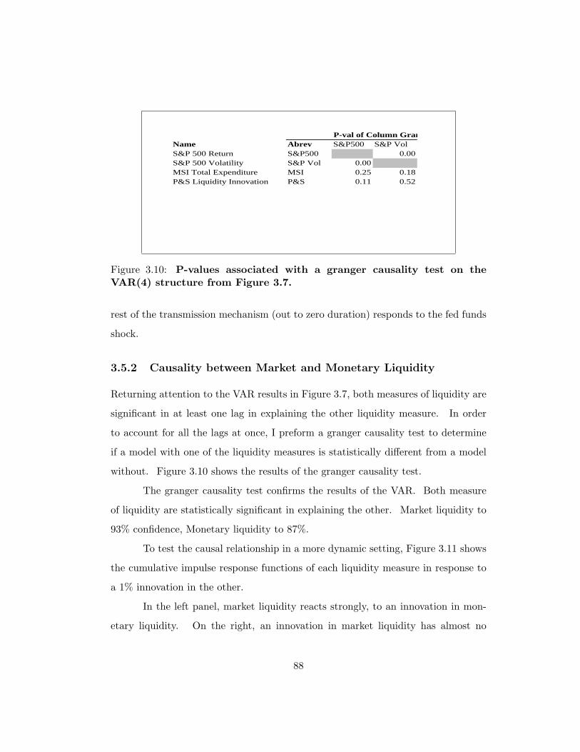
P-val of Column GranName Abrev S&P500 S&P VolS&P 500 Return S&P500 0.00S&P 500 Volatility S&P Vol 0.00MSI Total Expenditure MSI 0.25 0.18P&S Liquidity Innovation P&S 0.11 0.52

Figure 3.10: P-values associated with a granger causality test on theVAR(4) structure from Figure 3.7.

rest of the transmission mechanism (out to zero duration) responds to the fed funds

shock.

3.5.2 Causality between Market and Monetary Liquidity

Returning attention to the VAR results in Figure 3.7, both measures of liquidity are

significant in at least one lag in explaining the other liquidity measure. In order

to account for all the lags at once, I preform a granger causality test to determine

if a model with one of the liquidity measures is statistically different from a model

without. Figure 3.10 shows the results of the granger causality test.

The granger causality test confirms the results of the VAR. Both measure

of liquidity are statistically significant in explaining the other. Market liquidity to

93% confidence, Monetary liquidity to 87%.

To test the causal relationship in a more dynamic setting, Figure 3.11 shows

the cumulative impulse response functions of each liquidity measure in response to

a 1% innovation in the other.

In the left panel, market liquidity reacts strongly, to an innovation in mon-

etary liquidity. On the right, an innovation in market liquidity has almost no

88

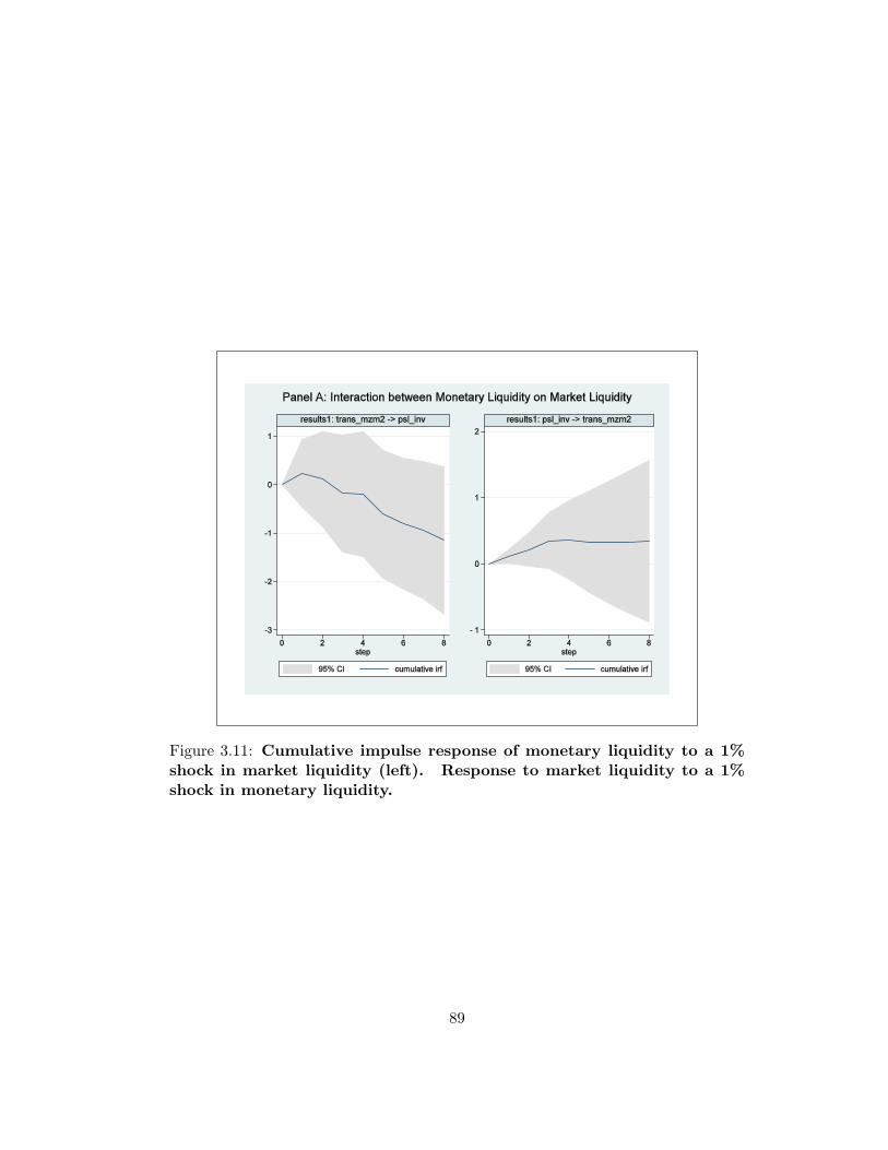
Figure 3.11: Cumulative impulse response of monetary liquidity to a 1%shock in market liquidity (left). Response to market liquidity to a 1%shock in monetary liquidity.

89

measurable impact on monetary liquidity.

From the VAR results we can conclude that while both market and monetary

liquidity have a measurable source of fundamental shocks to returns, market liquidity

does not on its own impact market volatility. Further, while there is statistical

evidence of joint causation between the two measures, the magnitude of the impacts

are such that monetary liquidity is a much larger fundamental shock.

3.6 Conclusion

The cost of liquidity is an important state variable for investors and consumers.

Previous attempts to measure the impact of liquidity on asset prices have focused

on market liquidity instead of monetary liquidity. This paper has shown that mar-

ket liquidity, while easily observable, overlooks a significant portion of fundamental

shocks that impact equity returns and volatility and are measured by monetary

liquidity. I have shown that using the monetary services index as a proxy for

liquidity can match the stylized facts of liquidity and asset prices as well or better

than existing market based measures of liquidity. While both measures explain

a significant portion of excess returns, only monetary liquidity contributes to ex-

plaining asset price volatility over time. Cross-sectionally, market liquidity is a

more easily measured systemic risk factor, but is completely undetectable after con-

trolling for changes in monetary liquidity. The impulse response function for a

Vector Auto Regression involving both measure of liquidly confirm the relative im-

portance of monetary liquidity. Additionally, they show that over time, innovations

to monetary liquidity contribute significantly to market liquidity, and the bulk of

causality should be attributed to monetary liquidity. The success of the MSI with

US data suggests that constructing a monetary services index for other countries

or across regions would provide an important measurement critical state variable of

the market.

90

Bibliography

Allen, Franklin and Douglas Gale, “Limited Market Participation and Volatility

of Asset Prices,” The American Economic Review, September 1994, 84 (4),

933–955.

Amihud, Yakov, “Illiquidity and stock returns: cross-section and time-series ef-

fects,” Journal of Financial Markets, January 2002, 5 (1), 31–56.

Anderson, Richard G., Barry E. Jones, and Travis E. Nesmith, “Monetary

Aggregation Theory and Statistical Index Numbers,” Federal Reserve Bank of

St. Louis, January 1997, 79 (1).

Azariadis, C. and Russell Cooper, “Nominal Wage-Price Rigidity as a Rational

Expectations Equilibrium,” The American Economic Review, May 1985, 75 (2),

31–35. Papers and Proceedings of the Ninety-Seventh Annual Meeting of the

American Economic Association.

Blinder, Alan S., “Indexing the Economy through Financial Intermediation,”

Carnegie-Rochester Conference Series on Public Policy, 1977, 5, 69–105.

Chordia, T. Sarkar and A. Subrahmanyam, “An Emperical Analysis of Stock

and Bond Market Liquidity,” The Review of Financial Studies, 2005, 18 (1),

85–129.

91

Diamond, Douglas W. and Philip H. Dybvig, “Bank Runs, Deposit Insurance,

and Liquidity,” The Journal of Political Economy, Jun. 1983, 91 (3), 401–419.

Dotsey, Michael, Robert G. King, and Alexander L. Wolman, “State-

Dependent Pricing and the General Equilibrium Dynmaics of Money and Out-

put,” The Quarterly Journal of Economics, May 1999, 114 (2), 655–690.

Dubra, Juan and Helios Herrera, “Market Participation, Information and

Volatility,” 2001. http://citeseer.ist.psu.edu/553379.html.

Fama, Eugene F. and James D. Macbeth, “Risk, Return, and Equilibrium:

Empirical Tests,” Journal of Political Economy, May/June 1973, 81 (3), 607–

636.

Freeman, Scott and G. Tabellini, “The Optimality of Nominal Contracts,”

Economic Theory, 1998, 11 (3), 545–562.

Lammoureux, C. and William D. Lastrapes, “Heteroskedasticity in Stock

Return Data: Volume versus GARCH Effects,” Journal of Finance, March

1990, 45 (1), 221–229.

Modiglianni, Franco and Merton H. Miller, “The Cost of Capital, Corporation

Finance and the Theory of Investment,” The American Economic Review, Jun.

1958, 48 (3), 261–297.

Nelson, E., “Direct Effects of Base Money on Aggregate Demand,” Journal of

Monetary Economics, May 2002, 49 (4), 687–708.

, “The Future of Monetary Aggregates in Monetary Policy Analysis,” Journal

of Monetary Economics, July 2003, 50 (5), 1029–1059.

Pagano, Marco, “Trading Volume and Asset Liquidity,” The Quarterly Journal

of Economcis, May 1989, 104 (2), 255–274.

92

Pastor, L. and Robert F. Stambaugh, “Liquidity Risk and Expected Stock

Returns,” Journal of Political Economy, June 2003, 111 (3), 642–685.

Watanabe, Akiko and Masahiro Watanabe, “Time-Varying Liquidity Risk

and the Cross Section of Stock Returns,” The Review of Financial Studies,

Forthcoming.

Willis, John, “Estimation of Adjustment Costs in a Model of State-Dependent

Pricing,” Federal Reserve Bank of of Kansas City Research Working Paper

00-07, December 2000. Available at SSRN: http://ssrn.com/abstract=272413.

93

Vita

Timothy Gordon Jones was born in Santa Monica, California on November 30th,

1978, son of Kenneth Moody Jones and Eileen Ann Jones. After completing his

studies at Piedmont High School, Piedmont, California, in 1996, he matriculated at

Yale University, New Haven, Connecticut. His senior thesis at Yale examined the

policy implications of a search model of unemployment. During the following years

he worked as a financial analyst for JPMorgan and NERA Economic Consulting.

In the Fall of 2003 he entered the graduate economics program at the University of

Texas.

Permanent Address: 4017 Vineland Drive, Austin, TX 78722

This dissertation was typeset with LATEX2ε4 by the author.

4LATEX2ε is an extension of LATEX. LATEX is a collection of macros for TEX. TEX is a trademark ofthe American Mathematical Society. The macros used in formatting this dissertation were writtenby Dinesh Das, Department of Computer Sciences, The University of Texas at Austin, and extendedby Bert Kay, James A. Bednar, and Ayman El-Khashab.

94