Copyright

by

Yang Gao

2016

The Dissertation Committee for Yang Gaocertifies that this is the approved version of the following dissertation:

Semiclassical Dynamics up to Second Order in Uniform

Electromagnetic Fields: Theory and Applications

Committee:

Qian Niu, Supervisor

Gregory A.Fiete

Chih-Kang Shih

Allan H.MacDonald

Lorenzo Sadun

Semiclassical Dynamics up to Second Order in Uniform

Electromagnetic Fields: Theory and Applications

by

Yang Gao, B.S.,B.S.,M.A.

DISSERTATION

Presented to the Faculty of the Graduate School of

The University of Texas at Austin

in Partial Fulfillment

of the Requirements

for the Degree of

DOCTOR OF PHILOSOPHY

THE UNIVERSITY OF TEXAS AT AUSTIN

May 2016

Dedicated to my parents, Yujun Gao and Sumei Pan.

Acknowledgments

Seven years is a significant period of time in life. Seven years ago, I

graduated from Peking University in China, imagining my next stage of life in

US. Now I am preparing my dissertation for doctorate degree. At this point,

I want to thank this wonderful opportunity granted by physics department at

University of Texas at Austin. Austin is such a great place to stay. I met a lot

of friendly people who were willing to help me to fit in. I also enjoy the warm

winter and lovely spring and fall. The barbecue is so good that after eating

some, even summer seems to be good.

More importantly, I am glad to stay in Professor Niu’s group for five

years and a half. Professor Niu is a wonderful advisor – knowledgeable, kindly,

and responsible. Doing research is always challenging. Well-formulated the-

ories I learned from textbook are like Plato’s imaginary Utopia, – they are

so perfect and beautiful that I sometimes doubted the meaning of my own

research and whether or not I can make any progress. At that time, Professor

Niu was very helpful and he would use a famous Chinese philosopher Yang-

ming Wang’s belief of knowledge as action to encourage me. I enjoy numerous

hours of discussion with him, which greatly helps me to not only make progress

in my research, but also establish real interest in physics. Moreover, I want to

especially thank his belief in me.

v

I want to thank delightful discussions with Xiang Hu, Shengyuan A.Yang,

Hua Chen, Ran Cheng, Xiao Li, and Zhenhua Qiao. They helped me to make

fewer mistakes in my research. I also want to thank Prof. Allan H.MacDonald

and Prof. Shengyuan A.Yang, who kindly agreed to write recommendation

letter for my postdoc application.

I want to thank my fiancee Wei, who helped me a lot during my difficult

time. I also thank my parents for their support and belief in me. Finally, I

want to thank all friends who helped me in these years.

vi

Semiclassical Dynamics up to Second Order in Uniform

Electromagnetic Fields: Theory and Applications

Publication No.

Yang Gao, Ph.D.

The University of Texas at Austin, 2016

Supervisor: Qian Niu

We derive a complete semiclassical theory up to second order with re-

spect to electromagnetic fields, by establishing the equations of motion for

the velocity and the force up to second order and modifying the band energy

up to second order. With this theory, we are able to calculate magnetoelec-

tric polarizability, nonlinear anomalous Hall conductivity, and the magnetic

susceptibility. Finally, we derive a density quantization scheme which is the

generalization of Onsager’s rule to any polynomial order, and show its theo-

retical and experimental implications.

vii

Table of Contents

Acknowledgments v

Abstract vii

List of Figures x

Chapter 1. Introduction 1

Chapter 2. Semiclassical Theory up to Second Order 4

2.1 General Background . . . . . . . . . . . . . . . . . . . . . . . . 4

2.2 First Order Semiclassical Theory . . . . . . . . . . . . . . . . . 7

2.3 Horizontal and Vertical Mixing . . . . . . . . . . . . . . . . . . 11

2.4 Positional Shift . . . . . . . . . . . . . . . . . . . . . . . . . . 14

2.5 Equations of Motion up to Second Order . . . . . . . . . . . . 16

Chapter 3. Magnetoelectric Coupling and Non-linear Anoma-lous Hall Effect 22

3.1 Magnetoelectric Coupling . . . . . . . . . . . . . . . . . . . . . 22

3.2 Non-linear Anomalous Hall Effect . . . . . . . . . . . . . . . . 26

Chapter 4. Static Magnetic Susceptibility at Zero field 33

4.1 General Theory . . . . . . . . . . . . . . . . . . . . . . . . . . 33

4.2 In Atomic Insulator Limit . . . . . . . . . . . . . . . . . . . . 38

4.3 Example I: Gapped Dirac Model . . . . . . . . . . . . . . . . . 45

4.4 Example II: Double Layer Graphene . . . . . . . . . . . . . . . 46

4.5 Example III: Tight-binding Graphene . . . . . . . . . . . . . . 53

4.6 Discussion . . . . . . . . . . . . . . . . . . . . . . . . . . . . . 58

viii

Chapter 5. Landau Level Quantization: Generalization of On-sager’s Rule 60

5.1 Onsager’s Rule and Berry Phase Correction . . . . . . . . . . . 60

5.2 Beyond the Berry Phase Correction . . . . . . . . . . . . . . . 64

5.3 Density Quantization Scheme . . . . . . . . . . . . . . . . . . 70

5.4 Application in continuum and lattice models . . . . . . . . . . 77

5.5 Experimental Implication . . . . . . . . . . . . . . . . . . . . . 81

Appendices 85

Appendix A. First Order Correction in the Wave-Packet 86

Appendix B. Band Energy up to Second Order 91

Publication List 95

Bibliography 96

ix

List of Figures

2.1 (color online) Schematic figure showing the horizontal mixingand the vertical mixing of Bloch states. . . . . . . . . . . . . . 12

3.1 (color online) Magnetoelectric Polarization in a 2D system witha mirror line along x axis. The mirror symmetry requires thezeroth order polarization P0 to be along the mirror line, andrequires the first order P ′ to lie in the perpendicular direction. 25

3.2 (color online) Modified Haldane model with a mirror line sym-metry to realize magnetoelectric coupling in 2D. The first argu-ment in the bracket for the second nearest neighbour hoppingis the hopping strength, and the second one is the phase due tothe local field. Phases in the upper and lower part of the cellhave opposite signs because they behave as the magnetic fieldunder reflection. . . . . . . . . . . . . . . . . . . . . . . . . . . 27

3.3 (color online) The electric nonlinear anomalous Hall effect in a2D system with a mirror line along x axis. The linear anoma-lous Hall current vanishes due to the mirror symmetry, but thenonlinear anomalous Hall current can exist along the mirror lineif the electric field is applied along the perpendicular direction. 29

4.1 (color online) Orbital magnetic susceptibility for the lattice model(4.31) as a function of µ. χ is in units of χ0 = e2a2t/(4π2~2), ais the bond length. Here ∆ = 0.2t, (a) t′ = 0 and (b) t′ = 0.1t.Here P-L, E Polar, and SP stand for the Peierls-Landau, energy-polarization, and saddle point, respectively. . . . . . . . . . . . 54

5.1 Zero-temperature electron density and its smooth interpolation. 72

5.2 (color online) The Hofstadter spectrum and the Landau levelenergy based on Eq.(5.46). We calculate three levels from theband bottom and two levels from the band top. . . . . . . . . 79

5.3 Comparing exact spectrum with the spectrum calculated fromthe quantization rule in Eq.(5.50) with Berry phase alone (〈m〉 =0 for Eq.(5.51)) and Berry phase plus magnetic susceptibilitycorrection. We calculate the spectrum for n = 1, n = 2, andn = 3 level. We use experimentally determined parametersm/m0 = 0.13, gs = 76, and vf = 3× 105m/s [76]. . . . . . . . 82

x

Chapter 1

Introduction

Ever since their discovery, geometrical concepts such as Berry phase

and Berry curvature are more and more important in the study of solid-state

physics, since they are related to a vast variety of response functions of Bloch

electrons. For example, the Chern number as obtained from the integration of

the Berry curvature, yields the quantum Hall conductivity, and opens a new

field of defining the states of matter. The Berry curvature is also essential

in understanding the spin/valley Hall effect, the anomalous Hall effect, the

magnetization, and so on, while the Berry phase finds its application in the

adiabatic pumping, Landau level quantization, modern theory of polarization,

and so on.

Among all those theories that use the Berry curvature and Berry phase,

the semiclassical theory is a particularly simple but powerful one. It interprets

the carrier in solids as a wave-packet of certain Bloch states, sharply localized

in k-space, and uses the center of mass position and gauge-invariant crystal

momentum of the wave-packet as the only dynamical variables 1 required to

describe the evolution of the wave-packet. The dynamics of this position and

1A new variable representing the internal degree of freedom may also appear if the wave-packet consists of Bloch states from multiple bands.

1

momentum is then obtained through the Euler-Lagrange equation from the

Lagrangian of the wave-packet. Compared with the textbook equations of

motion, an anomalous velocity is identified, manifesting as the cross prod-

uct of the force and the Berry curvature. Together with a correction to the

electronic density of states, it suggests a non-canonical structure in the elec-

tronic dynamics. Meanwhile, the electronic band energy is also modified by

a Zeeman-type energy due to the orbital magnetic moment, which completes

the semiclassical description of Bloch electrons up to first order in the elec-

tromagnetic field. This framework is well exemplified in various scenarios, as

summarized in [84].

However, one will need a semiclassical theory up to second order to

derive response functions such as the magnetoelectric polarizability, the mag-

netic susceptibility, the non-linear anomalous Hall conductivity, and so on.

The central work in this dissertation is thus how to accurately construct a

wave-packet for this semiclassical theory up to second order, and how to use

this theory to calculate the above mentioned response functions.

Our work is organized as follows. In Chapter 2, the semiclassical theory

up to second order is derived. One can see that the form of the equations of

motion stays the same, while the Berry curvature and the band energy are

corrected up to first and second order, respectively. In Chapter 3, the mag-

netoelectric coupling is derived, as an example to demonstrate the validity of

our theory. Moreover, the non-linear anomalous Hall conductivity is derived,

which can compete with the ordinary Hall effect in relatively dirty materials.

2

In Chapter 4, the semiclassical theory is used to study static magnetic suscep-

tibility from electronic orbital motion, and it offers a fresh understanding to

various mechanisms behind this complicated response function. In Chapter 5,

the Onsager’s rule is generalized, to incorporate not only the Berry phase and

magnetic moment correction, but also higher order magnetic responses, such

as the magnetic susceptibility. This generalized quantization scheme is due to

the quantization of semiclassical electron density, and have promising utility

both theoretically and experimentally.

3

Chapter 2

Semiclassical Theory up to Second Order

In this chapter, I will first review the background for the response func-

tions of Bloch electrons and the semiclassical theory to first order to calculate

it. Then I will present the semiclassical theory up to second order. 1

2.1 General Background

We are interested in the response functions of Bloch electrons to small

uniform external electromagnetic fields. The Hamiltonian for this problem

generally has the following form (we chose e and ~ to be unity):

H = H0(p+1

2B × q) +E · q . (2.1)

The difficulty to solve the above problem lies in the fact that direct perturba-

tion to the above Hamiltonian using the scalar and vector potential is invalid,

since those potentials are essentially unbounded.

There are many ways to avoid this difficulty, such as the standard

techniques to calculate response functions in the linear response theory [39,

1This semiclassical theory up to second order part (section 3,4,5) is based on the formal-ism part in Y.Gao, S. A. Yang, and Q. Niu, Phys. Rev. Lett.112, 166601 (2014) and Y.Gao, S. A. Yang, and Q. Niu, Phys. Rev. B 91, 214405 (2015) . This general formalism ofthe second order semiclassical theory is derived by me.

4

71, 25, 64, 65, 24, 78], the spatial perturbation technique [1, 29, 45, 68, 80,

5, 80, 48], and the semiclassical theory to be mentioned below. Among them,

we want to discuss a framework based on phase space quantum mechanics at

first, since it has a particularly simple physical structure (similar to Foldy-

Wouthuysen transformation in relativistic physics [21]), and is closely related

to the semiclassical theory we will discuss later.

This phase space quantum mechanics is first formulated by Moyal [50],

and later translated in the solid-state context by Blount [5, 6]. Its central idea

is to formulate the quantum mechanics using continuous phase space variables

p (momentum) and q (position) by constructing a distribution function from

the quantum mechanical state. The complete theory consists of three parts:

(1) it gives the distribution function in terms of p and q from the quantum

mechanical state; (2) it offers a systematic way to find a dynamics variable

O(p, q) in the phase space as the exact counterpart of the corresponding oper-

ator O(p, q) in the Hilbert space; (3) for any two dynamical variable O(p, q)

and T (p, q), one can define a Moyal star operation O(p, q) ? T (p, q) as an

asymptotic expansion over the commutator i[pi, qi] = ~, to exactly recover the

operator product O(p, q)T (p, q) in the Hilbert space.

In the solid-state context, under an external magnetic field, the mag-

netic field will modify the commutator in the following way: i[p1, p2] = ~B.

Therefore, the asymptotic expansion in the Moyal product is now with respect

to ~B, which is certainly valid at small B. With this understanding in mind,

the method of solving the dynamics from Eq.(2.1) can be easily constructed

5

based on the Foldy-Wouthuysen transformation: (1) find the Hamiltonian

Hnm(p, q) in the phase space, and the key to understand the dynamics is to

find a unitary transformation S to diagonalize Hnm(p, q) order by order (we

comment that the product operation in diagonalization is the Moyal product);

(2) based on the Bloch states |un(p)〉 at B = 0, one can construct the following

transformation matrix (S(0))nm(p,p′) = 〈un(p)|un(p′)〉, where |un(p)〉 is the

periodic part of the Bloch state; (3) then S = (S(0))nm(p + 12B × q, 0) can

diagonalize Hnm(p, q) at the leading order; (4) one can then find a series of

matrices S(i), which is of i-th order with respect to B, and the Moyal product

Πi`=0S

(`) is unitary up to i-th order; (5) it can be proved that the above con-

straint only determines the Hermitian part of S(i), and its anti-Hermitian part

is determined by requiring that Πi`=0S

(`) can diagonalize Hnm(p, q) up to i-th

order; (6) all other operators should transform accordingly based on Πi`=0S

(`).

With this complete understanding of the Hilbert space and operators,

one can in principle calculate any physical observable. In fact, Blount has

employed this formalism to analyze the orbital part of the magnetic suscepti-

bility [5]. However, the disadvantage of this formalism is that the phase space

variables p and q are canonical variables but not physical variables, so they

have the gauge-fixing issue (here the gauge refers to the U(1) transformation

of the Bloch states).

6

2.2 First Order Semiclassical Theory

The above phase space quantum mechanics formalism is closely related

to the semiclassical theory. In fact, it corresponds to the re-quantization of

the semiclassical theory. To demonstrate this, we will first introduce the semi-

classical theory up to first order [75, 84].

We start from constructing the wave-packet. For simplicity, we as-

sume that the chemical potential falls in one band labelled by 0, which is

well separated from other bands by a band gap. We note that this band 0

is from the local Hamiltonian obtained from the full quantum Hamiltonian

by evaluating the gauge potentials at the center of mass position rc of the

wave-packet, Hc(p, q) = H0(p + 12B × rc, q) + E · rc , where H0(p, q) is the

unperturbed Hamiltonian, p and q are momentum and position operators, and

we set e = ~ = 1 to simplify notations and use symmetric gauge in the vector

potential. Then the wave-packet for this problem only consists of Bloch states

from this band 0:

|W 〉 =

∫dpC0e

ip·q|u0〉 , (2.2)

where |u0(p + 12B × rc)〉 is the periodic part of the Bloch states. This wave-

packet is assumed to be sharply centered around some point pc in the Brillouin

zone, and subject to the constraint that the center of mass position of the

wave-packet coincides with the presumed value rc.

From this wave-packet, we can derive the Lagrangian up to first order

7

as follows:

L = 〈W |i∂t − Hc − H ′|W 〉 , (2.3)

where H ′ = 14mB · [(q− rc)× V − V × (q− rc)] +E · (q− rc) is the gradient

correction to the local Hamiltonian Hc. Obviously, this Lagrangian is only a

function of rc and pc. Since pc is not gauge-invariant under a magnetic field, we

can re-organize terms in L so that it is a function of rc and kc = pc+ 12B×rc,

both of which have clear physical meanings. We comment that using rc and

kc does not introduce any gauge issue, but it has a price that rc and kc are

generally non-canonical.

This non-canonical geometry of the semiclassical dynamics emerges in

the Euler-Lagrange equations of motion [75] based on L:

rc =∂ε

∂kc− kc ×Ω, (2.4)

kc = −E − rc ×B . (2.5)

where ε = ε0 − B ·m with ε0 being the band dispersion for band 0, m =

−12Im〈∂u0| × (ε0 − Hc)|∂u0〉 being the orbital magnetic moment in band 0,

and Ω = i〈∂u0| × |∂u0〉 being the Berry curvature in band 0. The second

term in the velocity is usually referred to as the anomalous velocity, and it

will introduce a factor 1 +B · Ω in front of the phase space volume element

drcdkc, which represents the violation of the Liouville’s theorem, and shows

the non-canonical nature between rc and kc.

The non-canonical structure in the dynamics can also be seen from the

8

connection between canonical and physical variables:

rc = q + a0 , (2.6)

kc = p+1

2B × q +B × (rc − q) , (2.7)

where a0 = 〈u0|i∂p|u0〉 is the Berry connection in band 0, p and q are canonical

variables. The appearance of a0 directly changes the Lie bracket between

different components of rc, and introduces the non-canonical structure.

Another way to understand the above semiclassical theory is by re-

quantizing it. By promoting the canonical variables in rc and kc and hence

in ε into the corresponding operators p and q, we essentially obtain an effec-

tive quantum mechanical theory for this single band problem, as discussed in

[13]. It is interesting to examine the wave function associated with this re-

quantization. Note that based on the wave-packet in Eq.(2.2), the Langrangian

in Eq.(2.22) can be put in the following form:

L =

∫dpC?

0(i∂t −H)C0 , (2.8)

where H is exactly ε after the above re-quantization. This coincidence implies

that C0 is the wave function acting by the Hamiltonian after re-quantizing

the semiclassical energy. Therefore, the semiclassical theory at first order is

actually a transformation from the local Bloch basis to this new basis spanned

by different C0 and this transformation is obviously unitary up to first order.

It is in this sense that the semiclassical theory is actually closely related to the

phase space quantum mechanics formalism discussed previously.

9

To make this relation more complete, we can examine the way the

position q and gauge-invariant crystal momentum p + 12B × q transform.

Based on the definition of rc, it is easy to prove that

〈W |q|W 〉 =

∫dpC?

0(i∂p + a0)C0 . (2.9)

Now we will focus on the crystal momentum p. p is related to the

translational operator TR as follows:

p = T−R(−i∂R)TR . (2.10)

Therefore, we have

〈W |p|W 〉 = 〈W |T−R(−i∂R)TR|W 〉

=

∫dpC?

0(p)C0〈u0(p+1

2B × rc)|

e−ip·qT−R(−i∂R)eip·Reip·q|u0(p+1

2B × (rc +R))〉

=

∫dpC?

0(p)C0〈u0(p+1

2B × rc)|

e−ip·qT−Rpeip·Reip·q|u0(p+

1

2B × (rc +R))〉

+

∫dpC?

0(p)C0〈u0(p+1

2B × rc)|

e−ip·qT−Reip·Reip·q(−i∂R)|u0(p+

1

2B × (rc +R))〉

=

∫dpC?

0(p)pC0(p) +

∫dpC?

0(p)1

2B × a0C0(p) . (2.11)

From the transformation p → p + 12B × a0, we know that p + 1

2B × q →

p+ 12B × i∂p +B × a0. Therefore, the transformation of q and p+ 1

2B × q

exactly coincides with the relation of rc and kc to canonical variables as shown

10

in Eq.(2.6). This is consistent with obtaining new operators from Πi`=0S

(`) in

the phase space quantum mechanics formalism.

2.3 Horizontal and Vertical Mixing

Despite of the success of the semiclassical theory up to first order, there

are many response functions which require a semiclassical theory up to second

order. For this purpose, the wave-packet in Eq.(2.2) is no longer appropriate.

Notice that from the connection between the semiclassical theory and the

phase space quantum mechanics formalism, the semiclassical theory up to

second order corresponds to applying a unitary transformation to remove the

first order interband matrix element in the Hamiltonian. This will inevitably

introduce the coupling between different bands. Therefore, the wave-packet

should be most appropriately constructed as follows:

|W 〉 =

∫dpeip·q

(C0|u0〉+

∑n6=0

Cn|un〉), (2.12)

where the interband mixing is directly added through Cn and |un〉. We com-

ment that Cn is of first order in electromagnetic field, since we only want to

remove the first order interband matrix element of the Hamiltonian.

Cn is connected to C0 by requiring that |W 〉 is a correct quantum

mechanical state:

i∂t|W 〉 = (H0 + H ′)|W 〉 . (2.13)

This constraint yields (see Appendix A for details):

Cn = −i12

[B × (i∂ + a0 − rc)C0] ·An0 −Gn0

ε0 − εnC0 , (2.14)

11

where Gn0 = −B ·Mn0 + E ·An0, Mn0 = 12(∑

m6=0 Vnm ×Am0 + v0 ×An0),

An0 = 〈un|i∂|u0〉 is the interband Berry connection, Vnm = 〈un|V |um〉 is the

velocity matrix element, and v0 ≡ V00. The subscripts n, m, and 0 are band

indices. ε represents the band energy. The partial derivative ∂ is with respect

to the crystal momentum.

There is another way to view this interband mixing from Cn. We can

renormalize the Cn|un〉 in Eq.(2.12) to |u0〉, and obtain the following modified

periodic part of the local Bloch state:

|u〉 = λ|u0(p+1

2B × q)〉+

∑n6=0

Gn0

ε0 − εn|un(p+

1

2B × rc)〉 , (2.15)

where λ is a normalization factor to ensure 〈u|u〉 = 1 to first order. It is

interesting to notice that the interband part in Eq.(2.12) actually has two

effects in this modified Bloch states in Eq.(2.15), and the one involving λ is

an intraband effect.

band 0

band n

p

E

horizontal mixing with

vertical mixing

p =1

2B (q rc)

Gn0

Figure 2.1: (color online) Schematic figure showing the horizontal mixing andthe vertical mixing of Bloch states.

12

We will first discuss the second term in Eq.(2.15). It consists of lo-

cal Bloch states at the same momentum from all the other bands (n 6= 0)

and respects the lattice translational symmetry. The essential quantity Gn0

is invariant under the U(1) gauge transformation to the Bloch states. Mean-

while, its form simply represents the coupling between electromagnetic fields

and interband matrix elements of electric and magnetic dipole moment. We

comment that Mn0 includes the time dependence of rc in the Bloch states,

which is in fact the nonadiabatic effect. The remaining part in B ·Mn0 is

from the interband part (An0) of the position operator q in H ′ in the Bloch

representation. We call this correction with Gn0 the vertical mixing since it

mixes Bloch states from different bands at the same k-point in the Brillouin

zone (as illustrated in Fig.(2.1)).

On the contrary, the first term in Eq.(2.15) only contains the Bloch

state inside the same band (band 0). Compared with the local Bloch state

|u0(p+ 12B × rc)〉, its crystal momentum is shifted to p+ 1

2B × q, suggesting

that the lattice translational symmetry is broken. We comment that this term

can be also obtained if we first take the position operator in the vector potential

in the exact Hamiltonian H as a c-number and later recover it in |u0〉 as an

operator. This shift of momentum is due to the intraband part of the position

operator q in H ′ in the Bloch representation. We comment that this intraband

correction to |u0〉 can be rewritten simply in terms of the shift of momentum

δp = 12B × (q − rc), and reads δp · D|u0〉, where D = ∂ + ia0 is the gauge-

covariant derivative acting on the Bloch states and a0 = 〈u0|i∂|u0〉 is the

13

intraband Berry connection. Since the correction from δp mixes Bloch states

at neighboring k-points in the same band, we call it the horizontal mixing.

In conclusion, the magnetic field affects the local Bloch states |u0〉 in

two ways: (i) it vertically mixes |u0〉 with the Bloch states |un〉 from other

bands; (ii) it also horizontally shifts the Bloch states along the path δp ac-

cording to the affine connection (Berry connection) a0 in the Brillouin zone.

We illustrate the two types of mixing of Bloch states schematically in Fig.2.1.

2.4 Positional Shift

As explained in the last section, in the second order theory, we need

to use |u〉 to construct the wave-packet. The difference between |u〉 and |u0〉

is that |u〉 contains the first order correction |u′0〉 from the gradient pertur-

bation H ′. Therefore, the wave-packet now acquires a shift in its center of

mass position given by a′0 = 〈u0|i∂p|u′0〉 + c.c.. It corresponds to a first or-

der correction to the Berry connection a0 = 〈u0|i∂p|u0〉 of the unperturbed

band, but is invariant under the U(1) gauge transformation to the local Bloch

states, as can be easily checked using the orthogonality between |u′0〉 and |u0〉.

Therefore it is a physical quantity and represents the shift of the wave packet

center due to external fields. Indeed, a′0 transforms as a spatial vector under

symmetry operations, e.g. it is odd under spatial inversion and even under

time reversal. This positional shift is the key concept in understanding the

semiclassical equations of motion up to second order.

From the wave-packet in Eq.(2.12), we can explicitly express this posi-

14

tional shift:

a′0 =∑n6=0

G0nAn0 + c.c.

(ε0 − εn)+

1

4∂i[(B ×A0n)iAn0 + c.c.] . (2.16)

The first term is due to the horizontal mixing, and the second term is due to

the vertical mixing. The above expression has another form:

a′i = FijBj +GijEj , (2.17)

where

Fij = Im∑n6=0

(Vi)0n(ωj)n0

(ε0 − εn)2, Gij = 2Re

∑n6=0

(Vi)0n(Vj)n0

(ε0 − εn)3, (2.18)

with ωn0 defined as

(ωj)n0 = −iεjk`∑m 6=0

[(Vk)nm + (vk)δnm](V`)m0

εm − ε0

. (2.19)

Here and hereafter, summation is implied over repeated spatial indices. Since

a′0 contains the interband velocity, it is not a single band property. All the

quantities in Eq.(2.18) can be readily evaluated in first principle calculations.

As a concrete example of the positional shift, we consider a generic

two-band model Hamiltonian with

H0 = h0 + h · σ (2.20)

where σ is the vector of Pauli matrices and h’s have arbitrary dependence on

the crystal momentum. The energy band dispersion is ε± = h0 ± h. Assume

15

the two bands are fully gapped with h 6= 0. The positional shift for the lower

band can be calculated from Eq.(2.17) and (2.18) with

Fij = −gikεk`j∂p`h0

4h− 1

8εjk`Γ`ki, Gij = − 1

4hgij, (2.21)

where gik = ∂pin · ∂pkn (with n = h/h) is the quantum metric of the band,

and Γ`ki = 12(∂pig`k + ∂pkg`i − ∂p`gki) is the corresponding Christoffel symbol

[3]. Like the Berry curvature, the quantum metric is also a geometric physical

quantity, which defines the infinitesimal distance in the Hilbert space on the

Brillouin zone. Meanwhile the Christoffel symbol defines the affine geometry

of the Brillouin zone [3]. They together make the Brillouin zone a Riemannian

manifold. It has been proposed that the quantum metric could be probed by

measuring the current noise spectrum [53]. Our result shows that g and Γ

are also closely connected with the positional shift, hence might be probed in

second order effects.

2.5 Equations of Motion up to Second Order

In this section, we will derive the correct equations of motion up to

second order and discuss its connection with the first order semiclassical theory.

From the wave-packet in Eq.(2.12) and using similar methods as in [75], we

find the following effective Lagrangian:

L = −(rc − a0 − a′0) · kc −1

2B × rc · rc − ε , (2.22)

where kc = pc + 12B × rc is the gauge invariant crystal momentum and ε is

the semiclassical energy accurate to second order. Its calculation needs the

16

second order gradient correction H ′′ = 18Γij[B × (q − rc)]i[B × (q − rc)]j to

the local Hamiltonian Hc, where Γij = ∂pipjH0 is the Hessian matrix. Its form

is given as follows (see Appendix B for details):

ε = ε0 −B ·m

+1

4(B ·Ω)(B ·m)− 1

8εsikεtj`BsBtgijαk`

−B · (a′0 × v0) +∇ · PE

+∑n6=0

G0nGn0

ε0 − εn+

1

8m(B2gii −BigijBj). (2.23)

Here Ω = −Im〈∂u0| × |∂u0〉 is the Berry curvature, m = −12Im〈∂u0| × (ε0 −

Hc)|∂u0〉 is the orbital magnetic moment, gij = Re〈∂iu0|∂ju0〉 − (a0)i(a0)j is

the quantum metric of k-space[3, 53], αk` = ∂k`ε0 is the inverse of effective

mass tensor, a′0 is the field-induced positional shift of the wave-packet center,

and PE = (1/4)[〈(B × D)u0|(V + v0) · |(B × D)u0〉 + c.c.] is a single band

quantity representing the energy polarization density in k-space. Indices i, j,

k, `, s and t refer to Cartesian coordinates and repeated indices are summed

over. εsik is the totally antisymmetric tensor in three dimension. For the

last term in Eq.(2.23), we choose Γij = δij/m (for Pauli and Schrodinger

Hamiltonians) for simplicity and a more general formula is given in Appendix

B. All physical quantities in Eq.(2.23) should be understood as functions of

the gauge-invariant crystal momentum kc, and the partial derivatives are with

respect to kc.

In Eq.(2.23), it is easy to check that each term is gauge-invariant. In

fact, they can be classified by their geometrical and physical meaning. The

17

first two terms in Eq.(2.23) have simple structures, and they are the band

energy plus the magnetic dipolar energy, which is expected based on the first

order semiclassical theory. We call the two terms in the second line the ge-

ometrical energies, since they consist of single band geometrical quantities,

i.e. the Berry curvature and the quantum metric. In the Brillouin zone, the

Hilbert space with single band Bloch states |u0〉 forms a fiber bundle, whose

curvature is characterized by the Berry curvature Ω [84], and the distance in

which is captured by the quantum metric[53]. For the remaining two quan-

tities, αkl depends only on the band dispersion and the magnetic moment m

is a single band quantity. It is interesting to note that αij and m actually

form a conjugate pair: they are proportional to the real and the imaginary

part of δij/m+2〈∂iu0|(ε0−Hc)|∂ju0〉, respectively. So are the quantum metric

and the Berry curvature, with respect to the quantity 〈∂iu0|∂ju0〉− (a0)i(a0)j.

Thus the less obvious meaning of gij and m can be understood from their well

studied conjugate partners Ω and αij.

The first term in the third line of Eq.(2.23) is a real space polarization

energy. It is due to the fact that the magnetic field shifts the wave-packet

center by a′0, and hence modifying the magnetic dipole moment. This modi-

fied magnetic dipole couples to the magnetic field to change the wave-packet

energy. The next term is a k-space polarization energy. This can be under-

stood by noticing that the the momentum shift δp gives rise to a second order

energy polarization in k-space, (1/2)(H ′δp + c.c.). Similar to the relation

between electric polarization and charge, the divergence of such energy polar-

18

ization yields a local energy correction. We find that this term is a single band

quantity, and is related to the quadrupole moments of the velocity operator.

In the fourth line of Eq.(2.23), the first term is a standard second

order perturbation energy through virtual interband transitions. The last

term in Eq.(2.23) is from the perturbation of H ′′. Note that this term vanishes

for the Dirac Hamiltonian, and for the nonrelativistic Pauli and Schrodinger

Hamiltonians, it comes with the bare electron mass m.

The above geometrical and physical meanings of the second order wave-

packet energy can also be implied from the vertical and horizontal mixings as

shown in Eq.(2.15). Such two types of corrections in |Ψ〉 originates from the

Bloch represention of H ′. Therefore, they enter the wave packet energy in

Eq.(2.23) through both H ′ and |Ψ〉. If two horizontal mixings are combined

to yield a second order energy, only the neighborhood in the Brillouin zone is

involved, and we should obtain a purely geometrical contribution as in the sec-

ond line in Eq.(2.23). On the contrary, if two vertical mixings are combined,

then virtual interband transition is involved, and we obtain an interband effect

as the first term in the fourth line of Eq.(2.23). If the horizontal and verti-

cal mixing are combined together, we obtain the k-space polarization energy,

which is a single band but not necessarily geometrical quantity.

By applying the Euler-Lagrangian equations of motion, we can obtain

19

the following dynamics from Eq.(2.22):

rc =∂ε

∂kc− kc × Ω , (2.24)

kc = −E − rc ×B , (2.25)

where Ω = ∇ × (a0 + a′0). To our surprise, compared with the first order

semiclassical dynamics in Eq.(2.4) and (2.5), these second order dynamics

possess exactly the same structure. The only differences are that the band

energy is now corrected up to second order as shown in Eq.(2.23) and that the

Berry curvature now has a first order correction as given by the curl of a′0. We

comment that this change of the Berry curvature does not affect the Chern

number. The reason is that a′0 is a physical vector and periodic in the Brillouin

zone, so the integration of its curl over the whole Brillouin zone vanishes. With

this equations of motion, one can easily derive the modification to the phase

space density of states, and it reads as 1 +B · Ω, i.e. we can simply change Ω

in the first order result by our new field-dependent Berry curvature Ω.

From the Lagrangian in Eq.(2.22), we can also derive the connection

between physical variables rc, kc and canonical variables q, p. The method

is that this connection can change L to a standard form: L = p · q − ε(p, q),

where ε is an appropriate energy. The result reads:

rc = q + a0 +1

2(B × a0 · ∂p)a0 +

1

2Ω × (B × a0) + a′0 , (2.26)

kc = p+1

2B × q +B × (rc − q) . (2.27)

Note that in Eq.(2.26) and (2.27), the argument for a0 and a′0 is p+ 12B × q.

Previously people thought that the first four terms on the right hand side

20

of Eq.(2.26) would be sufficient to first order in the fields [13], but now one

observes that this is incomplete without the positional shift a′0. We comment

that this relation can also be obtained by similar methods discussed in section

2.2.

21

Chapter 3

Magnetoelectric Coupling and Non-linear

Anomalous Hall Effect

With the equations of motion in Eq.(2.24) and (2.25), and the band

energy in Eq.(2.23), we obtain a complete semiclassical theory up to second

order. We can now use the free energy to obtain equilibrium response func-

tions and use the Boltzmann transport theory to obtain transport response

functions. As examples, in this chapter, we will derive the magnetoelectric

polarizability and the non-linear anomalous Hall effect from the semiclassical

theory up to second order. 1

3.1 Magnetoelectric Coupling

Usually when one applies a magnetic field, one expects a magnetiza-

tion based on the magnetic susceptibility. Similarly, electric field can induce a

polarization due to polarizability. However, the cross effect, namely the mag-

netization due to the electric field and the polarization due to the magnetic

1This chapter is based on Y.Gao, S. A. Yang, and Q. Niu, Phys. Rev. Lett.112, 166601(2014). My contribution is that I derive the general formalism and apply it to these twoapplications in the two-band model, and that I partially help to establish the conceptualunderstanding.

22

field is also possible. The corresponding response function is defined as the

magnetoelectric polarizability as follows [17, 18]:

αij =∂Pi∂Bj

=∂Mj

∂Ei, (3.1)

where P and M are polarization and magnetization, respectively. In multifer-

roics materials, this type of response function is usually mediated by phonons.

The purely electronic orbital part is derived in [18]. It consists of two contri-

butions, one is topological since it involves the integration of Chern-Simons

3-form, and the other one is cross-gap, since it involves virtual transition be-

tween occupied and unoccupied states. As a validity check of the semiclassical

theory, here we will show that it can be used to derive this electronic orbital

part of magnetoelectric effect.

The polarization in solids is obtained as follows [36]:

P =

∫dk

8π3a0 , (3.2)

where a0 is the Berry connection in one band. This can be understood based

on Eq.(2.6). The canonical position actually yields the lattice vector, which

should be discarded since the polarization is only well-defined up to lattice

vectors.

An external magnetic field will change this expression in two ways: (1)

the density of states is changed to 1 + B · Ω; (2) the Berry connection is

also changed according to Eq.(2.26). We take account these two changes, and

obtain the following formula from Eq.(3.2):

P ′ = −∫BZ

d3k

(2π)3

(1

2(Ω0 · a0)B + a′0

). (3.3)

23

The first term in Eq.(3.3) is the Chern-Simons 3-form for the Abelian

case, which is the essential quantity in the classification of three dimensional

topological insulators [59]. It only involves the Berry connection and Berry

curvature of the unperturbed band, and can be derived within the framework

of the first order semiclassical theory [17, 86]. An additional term from the

field-induced band mixing was envisioned in [86], but its calculation had to

wait for a full quantum perturbation formulation [18]. We now see that this

additional term has a very compact form of the positional shift integrated over

the Brillouin zone. Our results in Eq.(3.3) agrees exactly with the quantum

calculation, confirming the reliability of our semiclassical theory. Moreover, if

we apply our formula for the positional shift induced by an electric field, we

also get the correct result for the electric polarizability.

As an example, we will calculate the magnetoelectric polarization for

a generic two-band model in Eq.(2.20). The topological part (the first term

in Eq.(3.3)) is quantized and well understood [59, 60, 28, 31, 32, 22, 19, 42],

so we focus on the magnetoelectric polarization due to the positional shift,

which requires broken time reversal and spatial inversion symmetry [18]. For

the case of lower band being occupied, we have:

P ′µ =

∫d3k

8π3

gµνfν4h

=

∫d3k

8π3GµB . (3.4)

In the second expression, G = (4h)−1(z ·∂h0×∂ni)∂ni, with z being the direc-

tion of the magnetic field. We note that, if h0 is a constant G vanishes. This

is consistent with an earlier finding that a non-zero orbital magnetoelectric

polarization must break particle-hole symmetry [18].

24

From the symmetry analysis, one can build a minimal lattice model that

realizes this effect in 2D. Notice that for model Eq.(2.20) in 2D the topological

part of magnetoelectric polarization, i.e. the first term in Eq.(3.3) vanishes

[86] hence only the contribution from a′0 exists. Moreover, since a′0 transforms

as a spatial vector and it must lie in the plane, in general it must vanish if the

system has in-plane rotational symmetry. And if in-plane mirror symmetry

exists, P ′ would be restricted to be along the normal direction of the mirror

line (see Fig.3.1).

Figure 3.1: (color online) Magnetoelectric Polarization in a 2D system witha mirror line along x axis. The mirror symmetry requires the zeroth orderpolarization P0 to be along the mirror line, and requires the first order P ′ tolie in the perpendicular direction.

These symmetry constraints provide guidance for the construction of

the lattice model. The Haldane model with opposite onsite potentials on

two sublattices breaks the time reversal and spatial inversion symmetry, so it

may be a good candidate to realize such a system [27]. However, the original

25

Haldane model has three-fold rotational symmetry in the material plane, which

will suppress the orbital magnetoelectric polarization. So we change the local

magnetic field to break the rotational symmetry. The details of the model

are shown in Fig.3.2. Here the inter-sublattice hopping amplitudes (between

A and B sites) are equal to t1. The intra-sublattice hopping (between two

nearest A sites or B sites) has the same strength t2. However the phases of the

hopping depend on the local field and are subject to symmetry constraints.

Since under the in-plane mirror reflection, the magnetic flux behaves as the

magnetic field and will flip the sign. Without loss of generality, we adjust the

local field so that the upper two intra-sublattice hopping phases equal to φ for

the counterclockwise direction. Then the in-plane mirror symmetry requires

that the corresponding two lower hopping phases are −φ, and that the two

vertical intra-sublattice hopping phases vanish.

3.2 Non-linear Anomalous Hall Effect

The semiclassical dynamics can also be used to calculate the transport

current. Here we consider the intrinsic current which does not depend on the

transport relaxation time. The semiclassical current is defined by

j =

∫dk

(2π)3Drf0 , (3.5)

where D = 1 +B · Ω is the density of states, r is given in Eq.(2.24), and f0

is the equilibrium Fermi distribution function. It is important to note that

the argument of f must be the modified band energy ε as given in Eq.(2.23).

26

Figure 3.2: (color online) Modified Haldane model with a mirror line symmetryto realize magnetoelectric coupling in 2D. The first argument in the bracketfor the second nearest neighbour hopping is the hopping strength, and thesecond one is the phase due to the local field. Phases in the upper and lowerpart of the cell have opposite signs because they behave as the magnetic fieldunder reflection.

The reason is that under this Fermi function, the current that only depends

on B vanishes, as expected from the fact that the magnetic field alone does

not drive a current.

We want to derive the intrinsic contribution to the current. Therefore,

the distribution function f0 can be expanded as follows:

f0(ε) = f0(ε0) +∂f0

∂ε0

ε′

+∂f0

∂εε′′ +

1

2

∂2f0

∂ε2(ε′)2 + · · · , (3.6)

where ε′ = −B ·m is the first order correction to the semiclassical energy, and

ε′′ is the second order correction.

To derive the nonlinear anomalous Hall effect, we plug (3.6) into Eq.(3.5)

27

and keep the current at second order. The last two terms in Eq.(3.6) cancel

the corresponding terms in the center of mass velocity, i.e. the second order

correction to the wave packet energy does not enter into the final result. The

final result is clean and simple:

j ′ = E ×∫

[v0 × a′0 + Ω(B ·m)]∂f0

∂ε0

d3k

(2π)3. (3.7)

Or more explicitly we can write

∂2j′i∂Ej∂E`

=

∫(viGj` − vjGi`)

∂f0

∂ε0

d3k

(2π)3, (3.8)

∂2j′i∂Ej∂B`

=

∫(viFj` − vjFi` + εijkΩkm`)

∂f0

∂ε0

d3k

(2π)3, (3.9)

We call the two response functions in Eq.(3.8) and (3.9) the electric nonlin-

ear anomalous Hall effect and the magneto nonlinear anomalous Hall effect

respectively. We call such currents as anomalous because they are not caused

by the Lorentz force as in the case of the ordinary Hall effect. These response

functions can be directly evaluated by first principle methods.

From Eq.(3.5) we see that the intrinsic nonlinear current is normal to

the electric field, so it is purely of Hall type. Also, the appearance of ∂f0/∂ε0

shows that it is a Fermi surface property. The second term in Eq.(3.7) contains

only the Berry curvature and magnetic moment, so it can be derived from an

naive extension of the first order theory and has been discussed in the study

of anomalous Hall transport in multi-valley systems [9]. The first term comes

from the correction of the Berry curvature due to the positional shift found in

this work, so it can only be derived within the semiclassical theory up to second

28

order. We will show that this term is quite nontrivial. Moreover, we note that

for in-phase oscillating E and B fields, the first order intrinsic anomalous Hall

response vanishes upon time average, hence the DC intrinsic anomalous Hall

current would be dominated by the nonlinear response j ′.

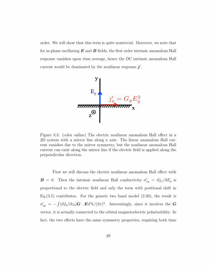
Figure 3.3: (color online) The electric nonlinear anomalous Hall effect in a2D system with a mirror line along x axis. The linear anomalous Hall cur-rent vanishes due to the mirror symmetry, but the nonlinear anomalous Hallcurrent can exist along the mirror line if the electric field is applied along theperpendicular direction.

First we will discuss the electric nonlinear anomalous Hall effect with

B = 0. Then the intrinsic nonlinear Hall conductivity σ′xy = ∂jx/∂Ey is

proportional to the electric field and only the term with positional shift in

Eq.(3.5) contributes. For the generic two band model (2.20), the result is

σ′xy = −∫

(∂f0/∂ε0)G · Ed3k/(2π)3. Interestingly, since it involves the G

vector, it is actually connected to the orbital magnetoelectric polarizability. In

fact, the two effects have the same symmetry properties, requiring both time

29

reversal and spatial inversion symmetries to be broken in the system. This

nonlinear anomalous Hall current will dominate if the corresponding linear

current vanishes due to symmetry constraint. For example, if a 2D system has

a mirror line perpendicular to the electric field, then the linear intrinsic current

vanishes because the (unperturbed) Berry curvature has a sign change under

mirror operation, while the nonlinear current could be finite (see Fig.3.3).

Now we discuss the magneto nonlinear anomalous Hall effect. It ac-

tually does not have such a stringent symmetry constraint, since the current

transforms in the same way as the product of electric and magnetic fields un-

der both time reversal and spatial inversion. So it is much easier to realize

in real systems. Furthermore, if the system itself has time reversal symmetry

(neglect the small Zeeman splitting due to the external magnetic field), both

the linear anomalous Hall effect and the electric nonlinear anomalous Hall ef-

fect vanish, and the magneto nonlinear anomalous Hall effect dominates. For

the two band model, we find that

σ′xy =

∫d3k

(2π)3

∂f0

∂ε0

[gij4h

(z × v)i (B × ∂h0)j

−1

8(z × v)iεk`jBkΓj`i + h(Ω · z)(Ω ·B)

], (3.10)

where v = ∂(h0 − h) and Ω = 12εijkni∂nj × ∂nk is the unperturbed Berry

curvature. As a concrete example, let’s consider a 2D gapped Dirac model with

h0 = 0 and h = (vkx, vky,∆), which is widely used to study systems such as

symmetry-breaking graphene, MoS2, topological insulator surfaces with time

reversal symmetry breaking, and topological insulator thin films [52, 85, 60,

30

28]. Here v is the fermi velocity and ∆ is the gap parameter. Then the first

term in Eq.(3.10) vanishes immediately due to the particle-hole symmetry.

Consider an in-plane electric field and an out-of-plane magnetic field, we obtain

that (at zero temperature)

σ′xy = −e3 v2(v2p2

F + 2∆2)

16π(v2p2F + ∆2)2

B , (3.11)

where pF = ~kF being the Fermi momentum and we assume the Fermi level is

in the upper band. We have recovered factors e and ~ in Eq.(3.11) to generate

the correct unit. In realistic materials, there may be valley degeneracy, such

as the inequivalent K and K ′ connected by time reversal symmetry in MoS2

or graphene (with inversion symmetry breaking), the contributions to this

magneto nonlinear anomalous Hall effect from the two valleys in fact add

together rather than cancel each other as in the first order response [88].

We comment that for magneto nonlinear anomalous Hall effect, since

both the electric field and magnetic field are applied (in a normal configu-

ration), there is also the ordinary Hall response due to Lorentz force. The

ordinary Hall conductivity also has a linear B dependence. However there is

an important difference. The ordinary Hall conductivity is proportional to

the square of relaxation time (or longitudinal conductivity), while our intrin-

sic nonlinear conductivity does not have such extrinsic dependence. On the

other hand, in terms of the Hall resistivity, the ordinary effect has an intrinsic

looking form ρordxy = −B/ne, where n is the carrier density, while intrinsic non-

linear Hall resistivity acquires a dependence on the square of the longitudinal

31

resistivity. This is well understood as a result of matrix inversion between the

conductivity and resistivity tensors with the usual condition that longitudinal

coefficients are much bigger than the transverse ones. Therefore from this

discussion, like the linear anomalous Hall effect, our nonlinear effect would

become important for more resistive samples.

As a concrete example of the difference between these two effects, we

consider the gapped Dirac model. From Eq.(3.11), we obtain the following

ratios between resistivities from these two effects

ρ′xyρordxy

=

(ρxx

e2

4h

)2[

1−(

∆

εF

)4], (3.12)

where εF =√v2p2

F + ∆2 is the Fermi energy, ρ′xy ' σ′xyρ2xx is obtained by in-

verting σ′xy, and ρxx is the longitudinal resistivity. In Eq.(3.12), the first factor

is proportional to ρ2xx, which is universal (model independent). The second

factor shows a simple dependence on Fermi energy for the gapped Dirac model:

it vanishes at the band bottom and quickly saturates with increasing Fermi

energies. Our predictions can be tested by the standard Hall bar measurement

on single layer MoS2 or Bi2Se3 thin films with longitudinal resistivity tuned by

temperature, film thickness, or doping. The difference in the scaling in terms

of the longitudinal resistivity as shown in Eq.(3.12) can be used to disentangle

the ordinary Hall effect and the nonlinear anomalous Hall effect.

32

Chapter 4

Static Magnetic Susceptibility at Zero field

In this chapter, I will formulate the general theory of static magnetic

susceptibility from my semiclassical theory. 1

4.1 General Theory

The magnetic susceptibility is a second order response function, defined

from the free energy density G by:

χij = − ∂2G

∂Bi∂Bj

. (4.1)

In atomic physics, various mechanisms for magnetic susceptibility are identi-

fied. They include the Pauli paramagnetic susceptibility, which is due to the

spin angular momentum of electrons, the Van-Vleck paramagnetic susceptibil-

ity, which is due to the interband transition induced by the magnetic vector po-

tential, the Langevin or Larmor diamagnetic susceptibility, which is due to the

second order perturbative Hamiltonian from the vector potential, and the Lan-

1This chapter is based on Y. Gao, S. A. Yang, and Q. Niu, Phys. Rev. B 91, 214405(2015). My contribution is that I derive the general formalism of the susceptibility andcalculate it to the honeycomb model and the dice lattice. I also derive the physical meaningof various contributions to the susceptibility.

33

dau diamagnetic susceptibility, which is purely due to the non-commutative

relation between different components of the mechanical momentum.

In the solid-state context, the Landau magnetism has been re-discovered

as the Peierls-Landau magnetism. It was later realized that unlike in the

atomic physics, the Peierls-Landau magnetism can be paramagnetic around

the saddle points inside the band [78]. The Pauli paramagnetism for spins is

easy to understand. However, other mechanisms are rather difficult to under-

stand.

The standard technique to calculate the magnetic susceptibility in-

cludes the linear response theory [39, 71, 25, 64, 65, 24, 78], and the spatial

perturbation technique [1, 29, 45, 68, 80, 5, 80, 48]. However, they have their

own disadvantages. The linear response theory can calculate the magnetic

susceptibility response as a whole, but it is rather difficult to identify different

mechanisms that contribute to this response function. So for each individual

materials, one has to calculate the susceptibility independently, and a univer-

sal understanding beyond each specific model is hard to establish. The spatial

perturbation technique is rather complicated in mathematics. Although it

is possible to envision mechanisms of susceptibility, as shown in [5], usually

canonical variables are involved in the derivation, which are not independent

of the choice of the phase of the Bloch state. This gauge issue comprises the

understanding of various mechanisms.

Our semiclassical theory up to second order as established in Chapter 2

is a good candidate to understand the complicated orbital part of the magnetic

34

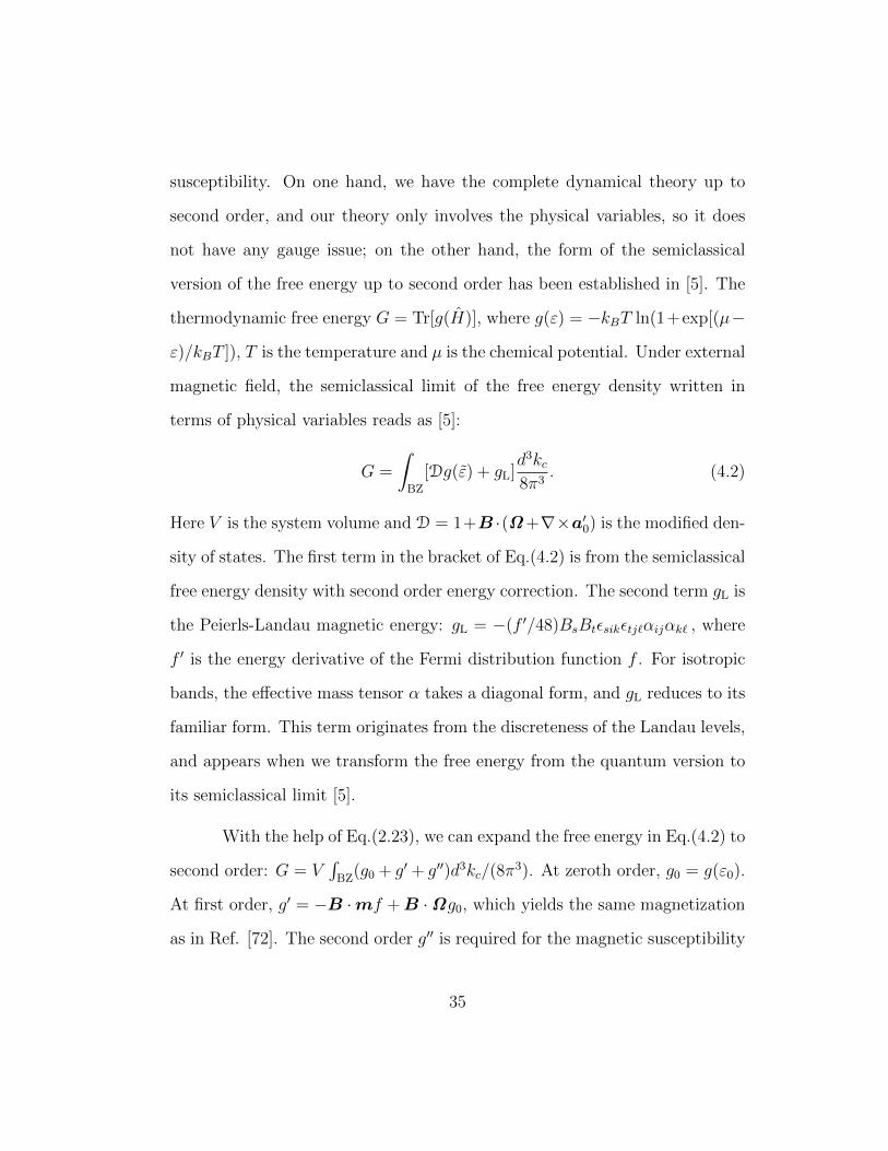
susceptibility. On one hand, we have the complete dynamical theory up to

second order, and our theory only involves the physical variables, so it does

not have any gauge issue; on the other hand, the form of the semiclassical

version of the free energy up to second order has been established in [5]. The

thermodynamic free energy G = Tr[g(H)], where g(ε) = −kBT ln(1+exp[(µ−

ε)/kBT ]), T is the temperature and µ is the chemical potential. Under external

magnetic field, the semiclassical limit of the free energy density written in

terms of physical variables reads as [5]:

G =

∫BZ

[Dg(ε) + gL]d3kc8π3

. (4.2)

Here V is the system volume and D = 1+B ·(Ω+∇×a′0) is the modified den-

sity of states. The first term in the bracket of Eq.(4.2) is from the semiclassical

free energy density with second order energy correction. The second term gL is

the Peierls-Landau magnetic energy: gL = −(f ′/48)BsBtεsikεtj`αijαk` , where

f ′ is the energy derivative of the Fermi distribution function f . For isotropic

bands, the effective mass tensor α takes a diagonal form, and gL reduces to its

familiar form. This term originates from the discreteness of the Landau levels,

and appears when we transform the free energy from the quantum version to

its semiclassical limit [5].

With the help of Eq.(2.23), we can expand the free energy in Eq.(4.2) to

second order: G = V∫

BZ(g0 + g′ + g′′)d3kc/(8π

3). At zeroth order, g0 = g(ε0).

At first order, g′ = −B ·mf +B ·Ωg0, which yields the same magnetization

as in Ref. [72]. The second order g′′ is required for the magnetic susceptibility

35

χij = −(1/V )(∂2G/∂Bi∂Bj)µ,T,V , and reads (for simplicity we take Γij =

δij/m)

g′′ = gL +f ′

2(B ·m)2 − f ′v0 · PE

+ fG0nGn0

ε0 − εn+

f

8m(B2gii −BigijBj)

− 3f

4(B ·Ω)(B ·m)− f

8εsikεtj`BsBtgijαk`. (4.3)

This second order free energy yields a susceptibility tensor as follows:

χst =f ′

24εsikεtj`αijαk` − f ′msmt

+f ′

4(εsikεtj` + εtikεsj`)(v0)k〈Diu0|(V + v0)`|Dju0〉

− (Mn0)s(M?n0)t + (Mn0)t(M

?n0)s

ε0 − εnf − f

4m(giiδst − gst)

+3f

4(Ωsmt + Ωtms) +

f

4εsikεtj`gijαk` . (4.4)

From Eq.(5.52), we find that the susceptibility only contains two types of

contributions, one from Fermi surface and the other one from Fermi sea. Mag-

netisms in the first line of Eq.(5.52) are contributions from the Fermi surface.

The first two contributions are the Peierls-Landau magnetism, and the Pauli

paramagnetism for the orbital moment m. In solids, the Peierls-Landau mag-

netism can be paramagnetic, especially near the band saddle points [78]. These

two contributions are prominent around singular points where the density of

states diverges. For example, around the saddle point, Peierls-Landau mag-

netism dominates in general [78]. The third term is due to the k-space energy

polarization in Eq.(2.23), and is first identified here. Similar to the Pauli and

36

Peierls-Landau magnetism, it also involves only single band quantities. This

term generally compete with the Pauli orbital and Peierls-Landau magnetisms

as illustrated in Fig.(4.1), except at the band maxima or minima where |v0|

vanishes.

The other terms in Eq.(5.52) are Fermi sea contributions. The first

term in the second line yields the Van Vleck susceptibility originated from

the vertical mixing energy in Eq.(2.23). It is due to the interband transition

from the vector potential, and is the only interband contribution to the orbital

magnetic susceptibility. It is always paramagnetic after summing over all the

occupied bands, similar to the Van Vleck paramagnetic susceptibility in atomic

systems. The second one yields a Langevin-like magnetic susceptibility from

the last term in Eq.(2.23). It can be expressed in a compact form using

the quantum metric gij, which describes the intrinsic fluctuation of position-

position operators (qiqj) in the Bloch representation: gij = Re[(Ai)0n(Aj)n0].

For Pauli or Schrodinger Hamiltonian with constant mass, this term yields

diamagnetic response along directions that diagonalize gij. Its expression will

change for effective Hamiltonians with a general Hessian matrix Γij as given in

Appendix B. For Dirac Hamiltonian, the Langevin-like magnetic susceptibility

vanishes.

Magnetic free energies in the third line in Eq.(5.52) have no analogs

as in atomic physics or for free particles, and are first identified here. We

call the susceptibility from these two terms the geometrical magnetic suscep-

tibility, because they are due to the geometrical energies in Eq.(2.23) from

37

the horizontal mixing of Bloch states and the geometrical correction to the

density of states in Eq.(4.2). Notice that the first term consists of the Berry

curvature, it is important when the band structure contains monopole or other

nontrivial topological structures. For example, for two band systems with the

particle-hole symmetry, geometrical magnetic susceptibility always yields a

diamagnetic susceptibility and is a prominent or even dominant contribution

in the band gap.

4.2 In Atomic Insulator Limit

A good way to understand various mechanisms of the magnetic suscep-

tibility in Eq.(5.52) is to examine various terms in the atomic insulator limit,

where the hopping between lattice sites is suppressed, and the lattice is simply

an array of atomic insulators. Then the susceptibilities in the second line in

Eq.(5.52) will reduce to the familiar Van Vleck paramagnetic susceptibility

and Langevin diamagnetic susceptibility in atomic physics. To demonstrate

this, we use the Wannier function representation. Notice that the periodic

part of the Bloch function can be expressed in terms of the Wannier function:

|un(kc)〉 =1√N

∑R

e−ikc·(r−R)|Wn(r,R)〉 , (4.5)

where n is the band index and |Wn(r,R)〉 is the Wannier function localized

at R for band n. With the help of Eq.(4.5), we can express the Van Vleck

paramagnetic susceptibility in terms of Wannier functions. To simplify the

discussion, we consider an insulator (with each band either completely filled

38

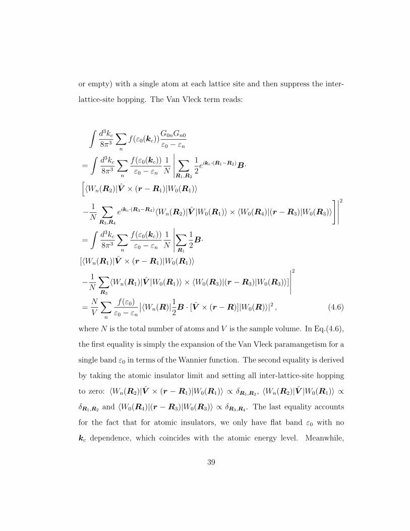
or empty) with a single atom at each lattice site and then suppress the inter-

lattice-site hopping. The Van Vleck term reads:

∫d3kc8π3

∑n

f(ε0(kc))G0nGn0

ε0 − εn

=

∫d3kc8π3

∑n

f(ε0(kc))

ε0 − εn1

N

∣∣∣∣∣ ∑R1,R2

1

2eikc·(R1−R2)B·[

〈Wn(R2)|V × (r −R1)|W0(R1)〉

− 1

N

∑R3,R4

eikc·(R3−R4)〈Wn(R2)|V |W0(R1)〉 × 〈W0(R4)|(r −R3)|W0(R3)〉]∣∣∣∣∣

2

=

∫d3kc8π3

∑n

f(ε0(kc))

ε0 − εn1

N

∣∣∣∣∣∑R1

1

2B·

[〈Wn(R1)|V × (r −R1)|W0(R1)〉

− 1

N

∑R3

〈Wn(R1)|V |W0(R1)〉 × 〈W0(R3)|(r −R3)|W0(R3)〉]∣∣∣∣∣2

=N

V

∑n

f(ε0)

ε0 − εn∣∣〈Wn(R)|1

2B · [V × (r −R)]|W0(R)〉|2 , (4.6)

where N is the total number of atoms and V is the sample volume. In Eq.(4.6),

the first equality is simply the expansion of the Van Vleck paramangetism for a

single band ε0 in terms of the Wannier function. The second equality is derived

by taking the atomic insulator limit and setting all inter-lattice-site hopping

to zero: 〈Wn(R2)|V × (r − R1)|W0(R1)〉 ∝ δR1,R2 , 〈Wn(R2)|V |W0(R1)〉 ∝

δR1,R2 and 〈W0(R4)|(r −R3)|W0(R3)〉 ∝ δR3,R4 . The last equality accounts

for the fact that for atomic insulators, we only have flat band ε0 with no

kc dependence, which coincides with the atomic energy level. Meanwhile,

39

〈W0(R3)|(r −R3)|W0(R3)〉 = 0, since the electron is bound with each atom

and its position expectation should coincide with the atom position. We also

use the fact that 〈Wn(R)|12B · [V × (r − R)]|W0(R)〉 are identical for all

lattice sites. It is easy to check that the final result in Eq.(4.6) is exactly the

Van-Vleck susceptibility in atomic physics.

By similar derivations, we find that the Langevin term in the atomic

insulator limit reads:∫d3kc8π3

∑n

f(ε0(kc))f

8m(B2gii −BigijBj)

=N

V

f(ε0)

8m〈W0(R)||B × (r −R)|2|W0(R)〉 , (4.7)

which is the familiar Langevin diamagnetic susceptibility in atomic systems.

Now we show that the geometrical magnetic susceptibility vanishes in

the atomic insulator limit. Therefore, our formula indeed reduces to the cor-

rect result in the atomic insulator limit. The first term of the geometrical

40

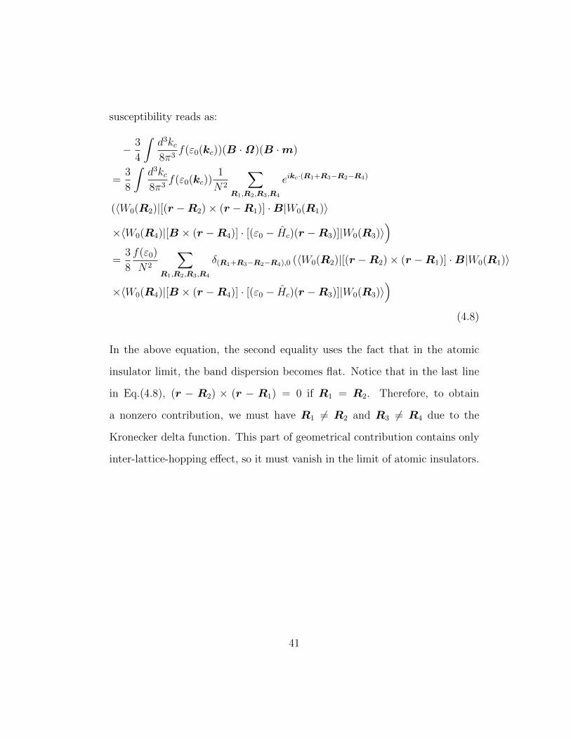
susceptibility reads as:

− 3

4

∫d3kc8π3

f(ε0(kc))(B ·Ω)(B ·m)

=3

8

∫d3kc8π3

f(ε0(kc))1

N2

∑R1,R2,R3,R4

eikc·(R1+R3−R2−R4)

(〈W0(R2)|[(r −R2)× (r −R1)] ·B|W0(R1)〉

×〈W0(R4)|[B × (r −R4)] · [(ε0 − Hc)(r −R3)]|W0(R3)〉)

=3

8

f(ε0)

N2

∑R1,R2,R3,R4

δ(R1+R3−R2−R4),0 (〈W0(R2)|[(r −R2)× (r −R1)] ·B|W0(R1)〉

×〈W0(R4)|[B × (r −R4)] · [(ε0 − Hc)(r −R3)]|W0(R3)〉)

(4.8)

In the above equation, the second equality uses the fact that in the atomic

insulator limit, the band dispersion becomes flat. Notice that in the last line

in Eq.(4.8), (r − R2) × (r − R1) = 0 if R1 = R2. Therefore, to obtain

a nonzero contribution, we must have R1 6= R2 and R3 6= R4 due to the

Kronecker delta function. This part of geometrical contribution contains only

inter-lattice-hopping effect, so it must vanish in the limit of atomic insulators.

41

Now we discuss the second term in the geometrical magnetic free energy.

− 1

8

∫d3kc8π3

f(ε0(kc))εsikεtj`BsBtgijαk`

=1

8

∫d3kc8π3

f(ε0(kc))εsikεtj`BsBt1

N2

∑R1,R2,R3,R4

eikc·(R1+R3−R2−R4)(R3 −R4)k(R3 −R4)`

〈W0(R4)|Hc|W0(R3)〉(〈W0(R2)|(r −R2)i(r −R1)j|W0(R1)〉

− 1

N

∑R3,R4

eikc·(R5−R6)〈W0(R2)|(r −R1)j|W0(R1)〉〈W0(R6)|(r −R5)i|W0(R5)〉)

=1

8

f(ε0)

N2εsikεtj`BsBt

∑R1,R2,R3,R4

δ(R1+R3−R2−R4),0

(R3 −R4)k(R3 −R4)`〈W0(R4)|Hc|W0(R3)〉〈W0(R2)|(r −R2)i(r −R1)j|W0(R1)〉 .(4.9)

Due to the prefactor (R3−R4), it is obvious that this remaining contribution

to the geometrical magnetic free energy also contains only inter-lattice-hopping

effect, so it also vanishes in the limit of atomic insulators.

Based on the above Wannier function representation of the magnetic

susceptibility, it is interesting to notice that the Fermi sea contribution to the

orbital susceptibility is due to two types of effects, i.e. intra-lattice-site transi-

tion similar to that in the atomic physics and inter-lattice-site hopping which

is unique in crystalline solids. Our classification in Eq.(5.52) thus provides

a reasonable extrapolation of the orbital susceptibility from atomic systems

to crystalline solids: on one hand, the Van Vleck paramagnetic susceptibility

and Langevin magnetic susceptibility reduce to their counterparts in atomic

systems and the geometrical magnetic susceptibility vanishes in the limit of

atomic insulators; on the other hand, even though they all contain inter-lattice-

42

site hopping contribution, the Van Vleck paramagnetic susceptibility and the

Langevin magnetic susceptibility in solids still preserve their essential prop-

erties established in the atomic systems, i.e. the Van Vleck paramagnetic

susceptibility is always paramagnetic and depends on the energy interval be-

tween two electronic states and the Langevin magnetic susceptibility is dia-

magnetic along directions that diagonalize the quantum metric. Furthermore,

we emphasize that the geometrical magnetic susceptibility is indeed unique in

crystalline solids and is a novel mechanism of orbital susceptibility that only

depends on the geometrical quantities in k-space.

In the above we have identified six different mechanisms to the orbital

magnetic susceptibility. Here we will argue that they can dominate in differ-

ent scenarios. In atomic systems, the Van Vleck paramagnetic susceptibility is

generally small due to the large separation between electronic levels, although

it has a notable exception in the atomic Lanthanide series, where the energy

interval between the ground state and the first excited states is small. In solids,

different energy levels can be very close, e.g. near the topological transition

points. In this case, the Van Vleck paramagnetic susceptibility become large.

However, we will show that in the circumstance where the linear band cross-

ing occurs, it is another contribution, i.e. the geometrical contribution, that

dominates over other orbital susceptibilities. The Langevin magnetic suscepti-

bility in atomic systems is also small and only important for close shell atoms.

Likewise, in solids the Langevin magnetic susceptibility is usually discussed

for insulators where electrons are localized. However, our theory suggests that

43

it is connected to the intrinsic expansion of the localized wave-packet, i.e.

the quantum metric. Therefore, for both insulators and metals, the Langevin

magnetism is well defined and can be sizable as discussed later. It can even

dominate over other susceptibilities as in the continuum model of the double

layer graphene.

In conclusion, within the wave-packet semiclassical approach, since the

Bloch electron energy is derived to second order in the magnetic field and clas-

sified into gauge-invariant terms with clear physical meaning as in Eq.(2.23),

it yields a fresh understanding of the complex behavior of orbital magnetic

susceptibility. We are able to answer the following questions: how the intrin-

sic geometry of Bloch bands affects the second order response to electromag-

netic fields, and whether or not there are additional geometrical quantities

emerging in the orbital magnetic susceptibility. We identify a geometrical

contribution from the Fermi sea, which we call the geometrical susceptibil-

ity, in the sense that it involves geometrical quantities including the Berry

curvature and the quantum metric. The geometrical susceptibility is a novel

mechanism for orbital magnetic susceptibility, which provides the dominant

diamagnetic response around the band gaps, and is especially important in

strongly spin/pseudospin-orbit coupled systems such as topological insulators

and 2D semimetals. We will present examples later.

Moreover, we derive a novel Fermi surface contribution, arising from

the energy polarization in the Brillouin zone, and competing with Pauli and

Peierls-Landau magnetism. To our delight, these Fermi surface contributions,

44

together with a Langevin-like magnetic susceptibility and the geometrical sus-

ceptibility, can be calculated based on Bloch states inside a single Bloch band,

and the only interband contribution is the Van Vleck paramagnetic suscep-

tibility. The various terms can dominate over different energy range of the

Bloch band, as illustrated later. We emphasize that the above understanding

of the orbital magnetic susceptibility is under the assumption of the mini-

mal coupling, in which case the magnetic field modifies the Hamiltonian only

through the magnetic vector potential. The generalization beyond the minimal

coupling assumption will be discussed later.

4.3 Example I: Gapped Dirac Model

The first example we choose is the gapped Dirac model. The model

Hamiltonian is given by:

H = vf (k1σ1 + k2σ2) + ∆σ3 , (4.10)

where vf is the Fermi velocity, and σ1, σ2, and σ3 are Pauli matrices. Using

Eq.(5.52) to calculate the susceptibility, we find that the energy polarization,

the Van-Vleck, and the Langevin susceptibility all vanish. So the only three

non-trivial contributions are:

µPL =∆2v2

f

8π|µ|3

µLD = −∆2v2

f

24π|µ|3

µCP = −∆2v2

f

12π|µ|3 , (4.11)

45

Here we assume the chemical potential µ falls inside the band (either valence or

conduction band). µPL, µLD, and µCP are the Pauli, Peierls-Landau, and the

geometrical susceptibility, respectively. One can see that these three contribu-

tions exactly cancel each other. The total susceptibility is 0 when µ falls inside

the band. However, when the Fermi energy falls in the gap, there will be a

diamagnetic susceptibility due to the geometrical susceptibility, and the Pauli

and Peierls-Landau susceptibility vanish since there are no Fermi surfaces.

An interesting fact is that the susceptibility satisfies the following sum

rule:∫χdµ = − v2

f

6π, which does not depend on the value of the band gap. At

the limit of ∆ → 0, the susceptibility when µ falls in the gap becomes larger

and larger, but it keeps zero when µ is in the band. Therefore, it gives a

delta-function type behavior for the susceptibility at ∆ = 0.

4.4 Example II: Double Layer Graphene

As the second example of our theory, we calculate the magnetic sus-

ceptibility in the low energy model of the double layer graphene. The model

Hamiltonian is given by

h =

(∆ − (k1−ik2)2

2m

− (k1+ik2)2

2m−∆

), (4.12)

where ∆ gives the band gap, and m is the effective mass.

We will first calculate the magnetic susceptibility from the Landau level

spectrum. The Landau level in the conduction band for this low energy model

46

is

εLL =

√∆2 +

B2

m2(n− 1/2)2 − B2

4m2, (4.13)

where n = 0, 1, 2, · · · .

We set x = (n− 1/2)B, then the free energy is

F = − 1

2πβ

∑n

ln(1 + e2βµ + eβµ(eβεLL + e−βεLL)

= − 1

2πβ

∫ ∞−B

ln(1 + e2βµ + eβµ(eβεLL + e−βεLL)dx+ FLD

FLD =B2

48πβ

βeβµ(eβεLL − e−βεLL)

1 + e2βµ + eβµ(eβεLL + e−βεLL)

x/m2√∆2 + x2/m2

∣∣x=∞x=0

=B2

48πm.

(4.14)

In the above equation, we have used the Euler-Maclaurin formula to trans-

form the summation over the Landau level index to the integration over the

continuous variable x. We only keep terms up to second order with respect to

B, since the susceptibility is a second order response function, and all higher

order terms do not contribute.

47

Therefore, the magnetic susceptibility is

χ = −∂2F

∂B2

∣∣B=0

=1

2π

∫ ∞0

eβµ(eβεLL − e−βεLL)

1 + e2βµ + eβµ(eβεLL + e−βεLL)

∂2ε

∂B2

∣∣B=0

dx− 1

24πm

= − 1

8πm2

∫ ∞0

1

ε

eβµ(eβεLL − e−βεLL)

1 + e2βµ + eβµ(eβεLL + e−βεLL)dx− 1

24πm

= − 1

8πm2

∫ ∞x0

1

εdx− 1

24πm

= − 1

8πm

∫ π/2

θ0

1

∆/ cos θ

∆

cos2 θdθ − 1

24πm

= − 1

16πmln

1 + sin θ

1− sin θ

∣∣π/2θ0− 1

24πm

= − 1

16πmln

1 + sin θΛ

1− sin θΛ

+1

16πmln

1 + sin θ0

1− sin θ0

− 1

24πm, (4.15)

where x = ∆m tan θ, θΛ corresponds to high energy cut-off, and ∆ = |µ| cos θ0.

Now I will calculate the susceptibility for the conduction band from

the semiclassical theory. Note that in the generic 2-band model H = h1σ1 +

h2σ2 + h3σ3, we have

h1 = −k21 − k2

2

2m

h2 = −k1k2

m

h3 = ∆ . (4.16)

Therefore, the wave function for the valence band is

ψ =1√

2ε0(ε0 −∆)

(h3 − ε0

h1 + ih2

). (4.17)

48

The Hessian matrix of the Hamiltonian are:

Γ11 = − 1

mσ1 , Γ22 = −Γ11 , Γ12 = − 1

mσ2 . (4.18)

Then the expectation of the Hessian matrix in the valence band is

〈ψ|Γ11|ψ〉 =h1

mε0

= −〈ψ|Γ22|ψ〉 , 〈ψ|Γ12|ψ〉 =h2

mε0

. (4.19)

Now we calculate a few important quantities used in Eq.(5.52) for the

magnetic susceptibility, including the Berry curvature Ω, the magnetic moment

mo, the density of states g(ε0) at the energy ε0, the inverse effective mass tensor

αij, the quantum metric gij. The results read:

Ω = − ∆k2

2m2ε30

m0 =∆k2

2m2ε20

g(ε0) =1

2π

mε0√ε2

0 −∆2

α11 =k2

2m2ε0

+∆2k2

1

m2ε30

α22 =k2

2m2ε0

+∆2k2

2

m2ε30

α12 =∆2k1k2

m2ε30

g11 =k2

4m2ε20

(1− k2k2

1

4m2ε20

)g22 =

k2

4m2ε20

(1− k2k2

2

4m2ε20

)g12 =

−k4k1k2

16m4ε40

. (4.20)

49

From the above quantities, various susceptibilities can be easily calcu-

lated. The Pauli paramagnetic free energy is

FPL = −1

2g(µ)B2m2

0 ⇒ χPL =∆2√µ2 −∆2

2πm|µ|3 . (4.21)

The Landau diamagnetic free energy is

FLD =1

24B2(α11α22 − α2

12)g(µ)

⇒ χLD = − 1

12

m|µ|2π√µ2 −∆2

[(k2

2m2ε0

+k2

1∆2

m2ε30

)(k2

2m2ε0

+k2

2∆2

m2ε30

)− ∆4k2

1k22

m4ε60

]= − 1

24π

m|µ|√µ2 −∆2

µ2 −∆2

m2µ2

(1 +

2∆2

µ2

)= − 1

24πm

√µ2 −∆2

|µ|

(1 +

2∆2

µ2

). (4.22)

The geometrical susceptibility due to the coupling of the density of

states and the magnetic dipole moment is:

χCP = 2

∫Ωm

d2k

4π2

= −∫

∆2k4

2m4ε50

dk2

4π

= −∫

∆2

πmε50

k4

4m2dk2

2m

= −∫ π/2

θ0

∆2∆2 tan2 θ

πm∆5/ cos5 θ

∆

cos2 θdθ

= − 1

πm

∫ π/2

θ0

sin2 θ cos θdθ

= − 1

3πm(1− sin3 θ0)

= − 1

3πm

(1− (µ2 −∆2)

√µ2 −∆2

|µ|3

). (4.23)

50

Now we calculate the second order energy. The geometrical energy from

the Berry curvature is:

1

4(B ·Ω)(B ·m) = − 1

16

B2∆2k4

m4ε50

= −1

4

B2∆2(ε20 −∆2)

m2ε50

. (4.24)

The geometrical term from the quantum metric is (notice that the effective

mass would pick up a minus sign for the valence band):

−1

8εθiαεφjβBθBφαijgαβ = −1

8(α11g22 + α22g11 − 2α12g12)B2

=1

8

B2k2

4m2ε20

[(1− k2k2

1

4m2ε20

)(k2

2m2ε0

+∆2k2

2

m2ε30

)+

(1− k2k2

2

4m2ε20

)(k2

2m2ε0

+∆2k2

1

m2ε30

)+k2k1k2

2m2ε20

∆2k1k2

m2ε30

]=

1

8

B2k2

4m2ε20

k2

2m2ε0

(1 +

3∆2

ε20

)=

B2

16m2

ε20 −∆2

ε30

(1 +

3∆2

ε20

). (4.25)

The first Heissian free energy is (there is a sign difference in the ex-

pecations of the Heissian for the conduction and valence band):

1

8

∑(m,n)6=0

(B ×A0m)i(Γij)mn(B ×An0)j =1

8εθiαεφjβBθBφ(Γij)ngαβ

=1

8((Γ11)ng22 + (Γ22)ng11 − 2(Γ12)ng12)B2

=1

8

B2k2

4m2ε20

[(1− k2k2

1

4m2ε20

)h1

mε0

−(

1− k2k22

4m2ε20

)h1

mε0

− 2k2k1k2

4m2ε20

h2

mε0

]=

1

8

B2k2

4m2ε20

(k2h2

1

2m2ε30

+k2h2

2

2m2ε30

)=B2

16

(ε20 −∆2)2

m2ε50

. (4.26)

51

Now we will calculate the second Hessian free energy:

− 1

16(B × ∂)i(B × ∂)j〈0|Γij|0〉 = −B

2

16(∂1∂1(Γ22)0 + ∂2∂2(Γ11)) − 2∂1∂2(Γ12)0)

= −B2

16∂2

(k2

m2ε0

− h1

mε20

k2k2

2m2ε0

)− B2

16∂1

(k1

m2ε0

+h1

mε20

k2k1

2m2ε0

)+B2

162∂1

(− k1

m2ε0

− h2

mε20

k2k2

2m2ε0

)= − B2

4m2ε0

(1− k4

4m2ε20

− 3k4

8m2ε20

+3k4

8m2ε40

k4

4m2

)= −∆2B2

4m2ε30

(1− 3(ε2

0 −∆2)

2ε20

)= −∆2B2

4m2ε30

3∆2 − ε20

2ε20

. (4.27)

Now we will sum up all the second order energy:

I = −∆2B2

4m2ε30

3∆2 − ε20

2ε20

+B2

16

(ε20 −∆2)2

m2ε50

+B2

16m2

ε20 −∆2

ε30

(1 +

3∆2

ε20

)− 1

4

B2∆2(ε20 −∆2)

m2ε50

=B2

8m2ε0

− ∆2B2(ε20 + 2∆2)

8m2ε50

. (4.28)

The corresponding susceptibility is

χI = −∫

1

4m2ε0

dk2

4π+

∫∆2(ε2

0 + 2∆2)

4m2ε50

dk2

4π

= − 1

8mπ

∫1

∆/ cos θ

∆

cos2 θdθ +

1

8mπ

∫∆2(∆2 tan2 θ + 3∆2)

∆5/ cos5 θ

∆

cos2 θdθ

= − 1

16πmln

1 + sin θ

1− sin θ

∣∣θΛθ0

+1

24πm(1− sin3 θ0) +

3

8πm

(1− sin θ0 −

1

3(1− sin3 θ0)

).

(4.29)

52

Combining Eq.(4.21), (4.22), (4.23) and (4.29), we obtain the total

susceptibility:

χ =1

2πmsin θ0 cos θ2

0 −1

24πmsin θ0(1 + 2 cos2 θ0)− 1

3πm(1− sin3 θ0)

− 1

16πmln

1 + sin θΛ

1− sin θΛ

+1

16πmln

1 + sin θ0

1− sin θ0

+1

24πm(1− sin3 θ0) +

3

8πm

(1− sin θ0 −

1

3(1− sin3 θ0)

)= − 1

16πmln

1 + sin θΛ

1− sin θΛ

+1

16πmln

1 + sin θ0

1− sin θ0

− 1

3πm+

1

24πm+

3

8πm− 1

8πm

+1

2πmsin θ0 −

1

24πmsin θ0 −

1

12πmsin θ0 −

3

8πmsin θ0

− 1

2πmsin3 θ0 +

1

12πmsin3 θ0 +

1

3πmsin3 θ0 −

1

24πmsin3 θ0 +

1

8πmsin3 θ0

= − 1

16πmln

1 + sin θΛ

1− sin θΛ

+1

16πmln

1 + sin θ0

1− sin θ0

− 1

24πm. (4.30)

This is the same result as obtained directly from the quantum mechanics.

4.5 Example III: Tight-binding Graphene

Our theory of magnetic susceptibility is not only valid for low energy

models, but also applicable in various realistic models, such as from first

principle calculations or the tight-binding approximations. Various terms in

Eq.(5.52) can readily be evaluated in first principle calculations. As a concrete

example to show how various terms contribute to the total magnetic suscepti-

bility and the importance of the geometrical magnetic susceptibility, we now

53

consider the following tight-binding model defined on a honeycomb lattice [52]:

H =− t∑〈i,j〉

c†icj − t′∑〈〈i,j〉〉

c†icj + ∆∑i

ξic†ici , (4.31)

where ci(c†i ) is the electron annihilation (creation) operator on site i, the first

and the second terms are the nearest-neighbor and second-neighbor hopping

terms, the third term is a staggered potential with ξi = ±1 for the two sublat-

tices, and t, t′ and ∆ are the strengths of the terms. The staggered potential

breaks the inversion symmetry and generates a gap of 2∆ in the spectrum. The

second-neighbor hopping is introduced for breaking the particle-hole symme-

try.

30

20

10

0

-10

-20

-2 -1 0 1 2 -2 -1 0 1 2

Pauli Orb.P-LE Polar.Van VleckLangevinGeom.Total

Pauli Orb.P-LLangevinGeom.Total

SP SPSP

SP

gap gap

(a) (b)

/

/ /

40

-30

Figure 4.1: (color online) Orbital magnetic susceptibility for the lattice model(4.31) as a function of µ. χ is in units of χ0 = e2a2t/(4π2~2), a is the bondlength. Here ∆ = 0.2t, (a) t′ = 0 and (b) t′ = 0.1t. Here P-L, E Polar,and SP stand for the Peierls-Landau, energy-polarization, and saddle point,respectively.

54

The various contributions to the orbital magnetic susceptibility are

plotted in Fig.4.1 with (a) and without (b) particle-hole symmetry. We first

consider the simple case with t′ = 0, such that the particle-hole symmetry is

preserved. Then the energy polarization and the Van Vleck contributions van-

ish identically, since Gn0 vanishes in any two band system with particle-hole

symmetry. From Fig.4.1(a), one observes that in the gap the Fermi surface

terms vanish and the geometrical magnetic susceptibility dominates, which

leads to a large diamagnetic response. The magnitude of the geometrical

magnetic susceptibility decreases rapidly away from the gap and it (along

with Peierls-Landau term) is compensated largely by the Pauli orbital para-

magnetic susceptibility which is peaked at the band edges where m takes its

largest value [9]. Two noticeable paramagnetic peaks are observed around the

band saddle points due to the Peierls-Landau contribution, which is a general

feature as discussed before [78]. Further away from the gap region, the sus-

ceptibility decreases gradually to zero. Our result of χ agrees with that from

the exact quantum treatment [64].

The physics around gap can be described by the gapped Dirac model

h = vk1σ1 + vk2σ2 + ∆σ3 with v = 3at/2 where a is the nearest-neighbor

bond length [52]. This model is widely used in the study of graphene, MoS2,

topological insulator surfaces and thin films [52, 85, 60, 28]. Here σ’s are the

Pauli matrices. Near the band edge (|µ| > ∆), the three competing mag-

netic susceptibilities have already been given in section 3, and the results can

well describe the susceptibility near the band edge. Moreover, we emphasize

55

that for systems with two valleys connected by time reversal operation, such

as graphene or MoS2, the geometrical magnetic susceptibilities from the two

valleys have the same sign. Note that in this low energy model the total sus-

ceptibility vanishes identically outside gap, which seems contradicting to the

result in Fig.4.1(a) where one sees a finite paramagnetic plateau. The differ-

ence is due to two Fermi sea contributions including the Langevin and a term

in geometrical magnetic susceptibility resulting from the nonzero Hessian Γij

(whereas Γij vanishes in the low energy model) which produce an overall shift

of χ. This was known as the “lattice contribution” in previous studies [25],

since it vanishes at the limit of a → 0 and t → ∞ with vf = ta a constant.

This agreement demonstrates the validity of our theory. We comment that

it is easy to show that the magnitude of this paramagnetic plateau does not

depend on the band gap. The value is same when the gap closes.

We point out that if one starts from the Pauli or Schrodinger Hamil-

tonian, the Langevin magnetic susceptibility is diamagnetic as discussed pre-

viously. But for an effective Hamiltonian as given in Eq.(4.31), the Langevin

magnetic susceptibility can be paramagnetic as shown in Fig.4.1. Therefore,

this paramagnetic plateau is sizable as in Fig.4.1 only when these two bands

are well separated from other bands such that the tight binding model is an

appropriate approximation.

Now we consider the case with a finite t′, such that the particle-hole

symmetry is broken. The results are shown in Fig.4.1(b), the geometrical

magnetic susceptibility still dominates in the gap and one notes that the para-

56

magnetic plateau near gap is suppressed in the valence band but enhanced in

the conduction band. Now the energy polarization and the Van Vleck con-

tributions are finite due to a finite Gn0. With current parameters, the Van

Vleck paramagnetic susceptibility takes a small value around the gap region,

while the energy polarization contribution takes opposite signs between the

two bands. The energy polarization term, along with the enhanced Langevin

and Pauli terms are the main contributions to a large paramagnetic response

between the conduction band edge and the saddle point. This is different from

the usual orbital paramagnetic susceptibility resulting from the Peierls-Landau

contribution [78]. In fact, the contribution from Peierls-Landau is less impor-

tant even in the region near and above the saddle point in conduction band.

The total susceptibility there is more affected by the competition between

geometrical, Langevin, and energy polarization terms. This is in contrast to

valence band where the Peierls-Landau dominates while other contributions

are suppressed.

This example illustrates that: (1) the geometrical magnetic suscep-

tibility is an important contribution, especially around the band gap; (2)

different terms in our classification dominate over different energy ranges;

(3) it is possible to enhance the paramagnetic susceptibility by breaking the

particle-hole symmetry. In addition, we note that for a generic two band model

h = h0 +h ·σ, Gn0 = −B · (∂h0×An0) is finite when particle-hole symmetry

is broken. From Eq.(5.52), we find that only the Van Vleck paramagnetic

susceptibility depends quadratically on ∂h0, while all other terms are either

57

independent or only have linear dependence. This implies that Van Vleck

susceptibility can in principle dominate for large |∂h0|, which also leads to a

strong paramagnetic response.

4.6 Discussion

Our theory could also be generalized beyond the minimal coupling.

Based on the Foldy-Wouthuysen transfromation in solid state context, the

correction beyond minimal coupling to the Hamiltonian is [21, 6]: ∆H =

B · µ + BihijBj, where µ and hij are appropriate matrix operators as func-

tions of (p+ 12B×rc). Then the expectation value of the second term directly

adds to the second order wave-packet energy, while the first term modifies the

orbital magnetic moment. For example, µ could stand for the electron spin

magnetic moment, whose diagonal and off-diagonal parts add to the corre-

sponding orbital moment m and Gn0, respectively.

In summary, based on the compact gauge-invariant expression of the

Bloch wave-packet energy as in Eq.(2.23) which is correct to second order in

external magnetic field, we obtain a complete and compact formula for the

orbital magnetic susceptibility, with important advantage that each term is

gauge invariant and has clear physical meanings. We find that other than the

familiar Pauli and Peierls-Landau magnetic susceptibilities, the orbital sus-

ceptibility in solids also consists of the Van Vleck paramagnetic susceptibility

and Langevin magnetic susceptibility, which reduce to their counterparts in

atomic physics in the limit of atomic insulators. More importantly, we identify

58

two new contributions: the geometrical magnetic susceptibility derived from

the Berry curvature and the quantum metric which can dominate in a small

energy gap, and the k-space energy polarization magnetic susceptibility, which

competes with Peierls-Landau and Pauli magnetic susceptibility on a Fermi

surface. These two susceptibilities will vanish in the atomic insulator limit,

so they are unique in the solid-state context. We illustrate that the Pauli,

Peierls-Landau and geometrical magnetic susceptibility depend solely on band

geometrical quantities and affect the orbital susceptibility greatly.

59

Chapter 5

Landau Level Quantization: Generalization of

Onsager’s Rule

5.1 Onsager’s Rule and Berry Phase Correction

Ever since the discovery of the quantum behavior from the black body

radiation, a fascinating subject is the connection between the quantum me-

chanics and the classical mechanics. Bohr and Sommerfeld established the

famous Bohr-Sommerfeld rule to generate the discrete energy levels in hydro-

gen atoms from the classical orbits with continuously varying energies. Then

Einstein envisioned a generalized version of the quantization rule for an inte-

grable dynamical system. He argued that the dynamics is actually described

by a series of invariant tories, which are determined by various action variables.

In the solid-state context, quantization of electronic states into Landau levels

by a magnetic field has particular importance, since it can cause oscillations

in magnetization (de Haas-van Alphen effect) and conductivity (Shubnikov-de

Haas effect), which contains a wealth of information about the band struc-

ture and geometric properties of Bloch states. Onsager translated the Bohr-

Sommerfeld rule into the Onsager’s rule [57] in the solid-state context, which

60

reads:

S = 2π

(n+

1

2

)eB

~, (5.1)

where S is the area enclosed by the semiclassical orbits in k-space. The shape

of Fermi surfaces of metals and semiconductors was obtained in this way.

However, later it was realized that this quantization rule has the fol-

lowing corrections:

S = 2π

(n+

1

2+ γ

)eB

~, (5.2)

where γ is some additional shift of the level index that depends on the magnetic

field and the constant of motion. The first order correction in γ has been found

to relate to the Berry phase. A good example is the Landau level near the

Dirac point in 2D monolayer graphene. The conduction band carries a uniform

Berry phase π, corresponding to γ = −1/2. Therefore, the Landau level starts

right from the Dirac point, where the energy is zero, different from the Landau

level of free electrons, which has a nontrivial zero-point energy. This shift of

Landau level index can be used to determine the Berry phase in such materials,

and the Berry phase in graphene has already been measured in this way.

However, the Berry phase correction can only yield the correct Landau

levels up to first order, not to arbitrary order. One can naively generalize this

Berry phase correction by correcting both the Berry phase and the band energy

to higher order, but this cannot generate Landau levels correct to higher orders.

As an example, we analyze the gapped Dirac model. The model Hamiltonian

is

H = vk1σ1 + vk2σ2 + ∆σ3 . (5.3)

61

If an magnetic field is applied along the z-direction, the hamiltonian is

H =

(∆ v(p1 − ip2 − 1

2By − i

2Bx)

v(p1 + ip2 − 12By + i

2Bx) −∆

). (5.4)

To exactly diagonalize the above Hamiltonian, we define

a† =1√2B

(p1 − ip2 −1

2By − i

2Bx) (5.5)

a =1√2B

(p1 + ip2 −1

2By +

i

2Bx) . (5.6)

Then it is easy to check that [a†, a] = 1. The eigenvalue satisfies:(∆− ε v(p1 − ip2 − 1

2By − i

2Bx)

v(p1 + ip2 − 12By + i

2Bx) −∆− ε

)(a1

a2

)= 0 , (5.7)

which gives

(∆− ε)a1 = v√

2Ba†a2 (5.8)

(−∆− ε)a2 = v√

2Baa1 . (5.9)

so the exact spectrum for the conduction band reads

εn =√

∆2 + 2v2Bn . (5.10)

Now we use the Berry phase correction to calculate Landau levels. The

semiclassical energy for the graphene system:

ε = ε0 −B ·m+B · v0 × a′0 +1

8αij(B ×A0n)i(B ×An0)j , (5.11)

62

where

ε0 =√

∆2 + v2k2 (5.12)

mz = −∆v2

2ε2(5.13)

αij = ∂ijε0 =

v2

ε

(1− v2k2

1

ε2

)−v4k1k2

ε3

−v4k1k2

ε3v2

ε

(1− v2k2

2

ε2

) (5.14)

The quantization rule with the Berry phase correction reads:

S = 2πeB

~

(n+

1

2− 1

2π

∮(a0 + a′0) · dk

). (5.15)

Here a′0 is the field induced positional shift, and it modifies the Berry connec-

tion and hence the Berry phase up to first order. For the case of graphene,

since the semiclassical energy up to second order (Eq.(9)) only depends on k2,

which means that the equal-energy surface is a circle. This fact will greatly

simplify the Landau level calculation. We get from the quantization rule that

k2 = 2πB

(n+

1

2+

1

2− ∆

2ε0

− 1

2π

∮a′0dk

). (5.16)

Inserting this quantization for k2 into the semiclassical energy Eq.(5.11).

The last term will vanish. The third term gets cancelled. The remaining part

is

ε = ε0 +∆Bv2

2ε20

. (5.17)

63

Then

ε0 =√

∆2 + v2k2 (5.18)

=

√∆2 + 2v2B(n+ 1)− v2∆B

ε(5.19)

= εn −v2∆B

2εnε− 1

8

v4∆2B2

ε3nε

2(5.20)

= εn −v2∆B

2ε2n

− v2∆2B2

4ε5n

− 1

8

v4∆2B2

ε3nε

2. (5.21)

The total energy would be

ε = ε0 +∆Bv2

2ε20

(5.22)

= εn −v2∆B

2ε2n

− v4∆2B2

4ε5n

− 1

8

v4∆2B2

ε3nε

2+

∆Bv2

2ε2n

+v4∆2B2

2ε5n

(5.23)

= εn +∆2B2v4

8ε5n

. (5.24)

Therefore, the semiclassical theory would miss a second order energy when

calculating the Landau level. Based on the definition of the magnetic suscep-

tibility, if the quantization rule is correct, this missing second order energy

should cause the semiclassical theory to fail to give the correct susceptibil-

ity. However, as discussed in the previous chapter, the susceptibility from the

semiclassical theory is exact. So the quantization rule must be modified.

5.2 Beyond the Berry Phase Correction

The above discrepancy finds its root in the very formulation of the

Bohr-Sommerfeld rule. The process of the Bohr-Sommerfeld rule, or its gen-

eral version the Einstein-Brillouin-Keller quantization rule, starts from the

64

observation that for a completely integrable system in d-dimension, there is

d constants of motion, which are the action variables in the action-angle for-

mulation of the classical mechanics. For simplicity, we consider the system

with one action variable J . Here in the Landau level quantization process,

J is proportional to the area enclosed by the semiclassical orbit in k-space.

Then we can write the modified energy ε as a function of J : ε = ε(J). The

right hand side of Eq.(5.2) chooses appropriate values of J for the Landau

level formation, which then yields the Landau level energy according to ε(J).

However, the above process is based on the assumption that operators

ˆε and ˆε(J) are the same, which cannot be taken a priori. Under the Landau

gauge for the magnetic vector potential, we can write the energy as ε(kx, ky +

Bx) and ε[J(kx, ky + Bx)]. If we directly promote the dynamical variable kx,

ky, x and y into operators kx,ky, x and y according to [x, kx] = [y, ky] = i~

and [x, ky] = [y, kx] = 0, it is easy to check that the operator ˆε(kx, ky + Bx)

is different from ˆε[J(kx, ky +Bx)], because they have different arrangments of

the two arguments kx and ky + Bx, which do not commute with each other

in the operator form. Actually, it has been long established in the phase

space quantum mechanics [50, 81], that the dynamical function ε(kx, ky +

Bx) corresponds to a quantum mechanical operator by re-arranging the two

arguments kx and ky + Bx into totally symmetric form and promoting them

into operators, which does not agree with the operator ˆε[J(kx, ky +Bx)] from

the Bohr-Sommerfeld rule in general.

As a concrete example, we illustrate how to correctly get the Landau

65

level up to second order for the gapped Dirac model, by adding the difference

between the operator ˆε(kx, ky + Bx) and ˆε[J(kx, ky + Bx)]. Notice that in

this model we can choose J = k2, and we label p = k + A where A is the

vector potential. Then we have [pi, pj] = εijkiBk. Quantum mechanically, p2p2

is different from pipj pipj. To get the right operator form we need to use the

total symmetric form for all the pi’s. The difference between two operators

A(pi)B(pi) and its total symmetric form is

<< AB >>=1

2i

(∂A

∂qi

∂B

∂pi− ∂A

∂pi

∂B

∂qi

)− 1

8

(∂2A

∂pi∂pj

∂2B

∂qi∂qj+

∂2A

∂qi∂qj

∂2B

∂pi∂pj− 2

∂2A

∂pi∂qj

∂2B

∂qi∂pj

)=iεijθBθ∂jA∂iB −

1

8BθBφεmθiεnφj

∂2A

∂ki∂kj

∂2B

∂km∂kn. (5.25)

For simplicity, we consider a rotational symmetric energy spectrum ε0(k). To

evaluate the exact difference in ε0, notice that ε0 = f(k2). We take the Laplace

transformation of ε0:

φ(s) =

∫ ∞0

f(x)e−xsdx . (5.26)

Then

f(x) =1

2iπ

∫ c+i∞

c−i∞φ(s)exsds . (5.27)

We can evaluate the difference in exs due to the noncommutability of x = k2:

esx = exs +∑n

sn

n!C2nx

n−2 << x, x >> (5.28)

+∑n

sn

n!C3nx

n−3 << x, x, x >> + · · · (5.29)

66

Finally, we can get

f(x) = f(x)− 1

8BλBµελ`kεµνρ

(1

2f ′′∂`νx∂kρx+

1

3f ′′′∂`νx∂kx∂ρx

). (5.30)

In general, we can change x into the action variable J , we have

ε(J) = ˆε− 1

8BsBtεsijεtk`

(1

2ε′′∂ikJ(k1, k2)∂j`J(k1, k2)

+1

3ε′′′∂ikJ(k1, k2)∂jJ(k1, k2)∂`J(k1, k2)

), (5.31)

where εsij is the totally antisymmetric tensor in three dimension. i, j, k, `, s

and t refer to Cartesian coordinates, and repeated index is summed. ε′′ and

ε′′′ is the second order and third order derivatives of ε with respect to J . Note

that the second term on the right hand side of Eq.(5.31) only involves J(k1, k2)

instead of J(k1, k2 +Bx).

The semiclassical theory has the energy corresponds to f(k1, k2), or the

operator from the total symmetrization of f(x(k1, k2)). However, the quanti-

zation we have done above corresponds to f(x). So we must take account the

difference between these two, which means that the exact Landau level from

the semiclassical theory should be

ε = εn +∆2B2v4

8ε5n

(5.32)

+1

8BλBµελ`kεµνρ

(1

2f ′′∂`νx∂kρx+

1

3f ′′′∂`νx∂kx∂ρx

). (5.33)

Since f(x) =√

∆2 + v2x and x = k2, we can calculate the energy. The result

is ε = εn +O(B3). Therefore, we have corrected the Landau level energy from

the semiclassical theory up to second order.

67

As a second example, we consider the low energy model in the dou-

ble layer graphene. The model Hamiltonian is given by H = −k21−k2

2

2σ1 −

k1k2σ2 + ∆σ3, where k1 and k2 are momentum in x and y direction, 2∆

is the band gap, and σ1, σ2 and σ3 are Pauli matrices. Under a B field

along z direction, Landau levels in the conduction band can be solved exactly:

εquan =√

∆2 + n(n− 1)B2, with n = 0, 1, 2, · · · .

To apply the Onsager’s rule, we start with the band energy modified

by the magnetic field. We will focus on the conduction band. According to

the discussion in Chapter 4 and given that this model has the particle-hole

symmetry, the band energy up to second order in B for the conduction band

reads:

ε = ε0 −Bm+1

4(B ·Ω)(B ·m)− 1

8εsikεtj`BsBtgijαk` −B · (a′0 × v0)

+1

8

∑(m,n) 6=0

(B ×A0m)i(Γij)mn(B ×An0)j −1

16(B × ∂)i(B × ∂)j(Γij)00 .

(5.34)

Here ε0 is the conduction band dispersion without any magnetic field, m = ∆k2

2ε20

is the orbital magnetic moment; Ω = ∆k2

2ε30is the Berry curvature; gij is the

quantum metric tensor:

g =k2

4ε20

(1− k2k2

1

4ε20−k2k1k2

4ε20

−k2k1k2

4ε201− k2k2

2

4ε20

); (5.35)

αk` is the effective mass tensor:

α =

(k2

2ε0+

∆2k21

ε30

∆2k1k2

ε30∆2k1k2

ε30

k2

2ε0+

∆2k22

ε30

); (5.36)

68

v0 = k2

2ε0(k1, k2) is the band velocity; a′0 is the field induced positional shift:

a′0 =(k2,−k1)

2ε20

(1− 3k4

8ε20

)B ; (5.37)

A0m is the interband Berry connection; Γij = ∂ijH is the Hessian matrix.

Therefore, we can obtain the modified band energy up to second order

in B:

ε = ε0 −B∆k2

2ε20

− B2

8ε0

(1− ∆2(ε2

0 + 2∆2)

ε40

)− k4B2

4ε30

(1− 3k4

8ε20

). (5.38)

Obviously, the equal-energy contour of ε is a circle, and its area is

S = πk2. From the Onsager’s rule, we obtain that

S = 2π

(n+

1

2− Γ(µ)

2π

)B , (5.39)

where Γ =∮

(a0 + a′0) · dk is the Berry phase up to first order in B, and

n = 0, 1, 2, · · · . The Berry phase contribution from a0 is∮a0 · dk =

∫Ωd2k = 2π

(1− ∆

ε0

). (5.40)

The field induced positional shift a′0 yields:∮a′0 · dk = −πBk

2

ε20

(1− 3k4

8ε20

). (5.41)

Based on Eq.(5.39-5.41), we have

πk2 = 2π

[n− 1

2+

∆

ε0

+k2B

4ε20

(1− 3k4

8ε0

)]B. (5.42)

We then plug Eq.(5.42) into Eq.(5.38) to obtain the Landau level energy

ε from the Onsager’s rule. The exact Landau level energy εquan has been given

69

in the main text. We will expand the difference between ε and εquan up to

second order in B:

ε =

√ε2

quan +B2

4+

∆2B2

ε20

+2∆(n− 1/2)B2

ε0

− ∆Bk2

2ε20

− B2

8ε0

(1− ∆2(ε2

0 + 2∆2)

ε40

)= εquan +

∆2B2

2ε3quan

+∆B2(n− 1/2)

ε2quan[1 + ∆B2(n− 1/2)/(ε3

quan)]− ∆2B4(n− 1/2)2

2ε5quan

− ∆B

2

2(n− 1/2 + ∆/εquan)B

ε2quan[1 + 2∆B2(n− 1/2)/(ε3

quan)]+B2∆2(ε2

quan + 2∆2)

8ε5quan

+O(B3)

= εquan +∆2B2

8ε5quan

(ε2quan − 2∆2) +O(B3) . (5.43)

Therefore, the Onsager’s rule is not guaranteed to produce correct Landau

levels even with the higher order Berry phase and band structure corrections.

By adding the correction in Eq.(5.31), the second term in the last line of

Eq.(5.43) will be cancelled, and we have the correct Landau level up to second

order.

5.3 Density Quantization Scheme

There is a systematic way to generalize the Onsager’s rule to any order

of magnetic field. It is given by the quantization of the semiclassical elec-

tron density at zero temperature. In this section, we will derive this density

quantization scheme.

Without loss of generality we derive the quantization rule in two di-

mension. We start from the observation that each Landau level carries the

same density of states in two dimensional electron gas. It is well known that

70

when the Fermi energy falls between neighboring Landau levels in two dimen-

sional electron gas, the transverse conductivity is quantized (the quantum Hall

effect): σtrans = ne2/h, where n is an integer called Landau level filling factor.

The transverse current from this conductivity can also be derived by multiply-

ing the density of states ρ with the drift velocity: j = eρ(E ×B)/B2, where

E is in-plane electric field and B is out-of-plane magnetic field. Therefore,

the density of states is also quantized ρ = neB/h, and each Landau level has

the same density of states eB/h.

Similar observation also holds for crystalline solids, where the Hofs-

tadter spectrum emerges instead of Landau levels. When the Fermi energy falls

in the spectral gap, the carrier density ρ reads as [79, 46, 14]: ρ = nB/φ0+t/A,

where φ0 = h/e is the magnetic flux quantum, A is the unit cell area, n is an

integer connected to the quantum Hall effect, and t is an integer connected to

the filling index in the mini-band. We will focus on the case with t = 0 due to

the following recursive structure in the Hofstadter butterfly[11, 30, 79, 46, 14]:

for the ‘pure case’ with a flux φ/φ0 = 1/q (φ = BA and q is an integer),

t = 0 and the spectrum generally follows a set of Landau levels arising from

the original band structure at B = 0; on the other hand, for the situation

with φ/φ0 = p/q (p and q are co-prime integers) with 1 < p < q/2, the

spectrum can be renormalized to a pure case arising from the magnetic Bloch

band at a certain rational flux φ′, and the flux is renormalized to φ − φ′

with (φ − φ′)/φ0 = 1/q′ (q′ is an integer). Therefore, the carrier density is

ρ = nB/φ0 and each mini-band in the Hofstadter spectrum carries the same

71

density of states eB/h.

The Landau level spectrum εn(B) (level index n = 0, 1, · · · ) from a band

minimum in two dimensions can be expressed as ρ(B, T, µ) = (B/φ0)∑

n f [εn(B)−

µ] with φ0 = h/e the flux quantum, f the Fermi function and µ the chem-

ical potential. At T = 0, according to above analysis, the electron density

is a staircase function with constant risers B/φ0 located at µ = εn(B) (see

Fig.(5.1)).

Electron density Smooth Interpola4on Midpoints

µ

Figure 5.1: Zero-temperature electron density and its smooth interpolation.

The spectrum εn(B) can be interpolated as follows. Without loss of

generality, we write εn(B) = g(xn, B) with xn = (n + 1/2)B/φ0 being the

zero-temperature electron density when the n-th Landau level is half-filled. If

we allow x change continuously, the function ε = g(x,B) smoothly interpolate

points εn(B) at x = xn for each value of B. g(x,B) is a monotonic function of

x for each B, inherited from the fact that εn(B) increases with n. Therefore,

72

we can invert g(x,B) and obtain x = x(µ,B), represented as the smooth

curve in Fig.(5.1). By construction, the interpolation condition implies that

this smooth curve goes through the midpoints of the staircase risers.

In the following, we will show that the smooth interpolation curve

x(µ,B) is actually the semiclassical electron density ρsemi(B, T → 0, µ). Notice

that there are three energy scales in the exact electron density ρ(B, T, µ): the

Landau level spacing determined byB, the variation scale of the Fermi function

determined by kBT , and the chemical potential µ. We assume µ falls inside

the band, and thus has a finite distance from the band minimum. To calcu-

late finite temperature semiclassical electron density ρsemi(B, T, µ), we set the

level spacing to be much smaller than kBT . Then, using the Euler-Maclaurin

formula, we can transform the sum over n in ρ(B, T, µ) to an integration over

a continuous variable x:

ρsemi(B, T, µ) =

∫ ∞B/2φ0

fdx+Bf |x=B/2φ0

2φ0

+ R , (5.44)

where f = f [g(x,B)− µ]. R contains all the remainder terms.

Eq.(5.44) can be greatly simplified. Terms in R are evaluated at x =

B/2φ0, i.e. at the 0-th Landau level near the band minimum. Here we have

ignored the contribution at x =∞ since they correspond to very high energy,

and this is still valid for realistic models in solid state physics which contain

singular points. Moreover, terms in R are proportional to successively higher

power of B and contain ∂f/∂µ and its higher order derivatives with respect

to µ. The limit T → 0 in ρsemi(ρ, T → 0, µ) is understood as kBT being

73

much smaller than the distance between µ and band minimum, but still much

bigger than the level spacing. Therefore, each term in R is exponentially

small. At this limit of kBT → 0, Eq.(5.44) may not converge, in which case

it is understood as an asymptotic expansion. Therefore, we can keep finite

number of terms in Eq.(5.44) and then set kBT → 0. The result is simply

ρsemi(B, T → 0, µ) = x(µ,B).

The coincidence between the interpolation curve x(µ,B) and the semi-

classical electron density at the limit of zero temperature yields a density

quantization scheme:

ρ(B, T → 0, εn) = xn . (5.45)

At finite temperature, we have the following power series expansion: for any

N ≥ 0, ρsemi(B, T, µ) =∑N

m=0 Rm(µ, T )Bm/m! + O(BN+1), where Rm(µ, T )

is the zero-field response function defined from the exact electron density

ρ(B, T, µ) by Rm(µ, T ) = limB→0 ∂mρ/∂Bm. At T → 0, we treat the above ex-

pansion in the asymptotic sense, and obtain ρsemi(B, T → 0, µ) =∑N

m=0Rm(µ, T →

0)Bm/m!+O(BN+1). Application of the interpolation condition xn = x(εn, B)

to this expression then yields(n+

1

2

)B

φ0

=N∑m=0

Rm(εn, T → 0)Bm

m!+O(BN+1) . (5.46)

Eq.(5.46) is our density quantization scheme: we first calculate Rm(µ, T → 0)

from the semiclassical theory, and then solve the spectrum εn from Eq.(5.46).

Obviously, this spectrum can be accurate to arbitrary order of B as long as

corresponding Rm(µ, T → 0) are given.

74

We comment that these Rm(µ, T → 0) are connected to the response

of the smooth semiclassical free energy G(B, µ, T → 0) with respect to B.

Here and hereafter, we use Rm to represent Rm(µ, T → 0). Based on the

Maxwell relation, we have R0 = ∂G|B=0/∂µ, R1 = ∂M/∂µ, R2 = ∂χ/∂µ, · · · ,

where M = −(∂G/∂B)|B=0 is the magnetization, χ = −(∂2G/∂B2)|B=0 is the

susceptibility, and so on.

Eq.(5.46) is our new quantization rule and we demonstrate its signifi-

cance through its relation with the Onsager’s rule. First, we truncate its right

hand side at the zeroth order term. Since R0 = S0/(4π2) where S0 is the

k-space area enclosed by the equal-energy contour in the band structure ε0

with the energy µ, we obtain the Onsager’s rule: S0 = 2π(n+ 1

2

)eB~ .

Then we truncate Eq.(5.46) at the first order term BR1 = B∂M/∂µ.

We consider the spinless case for simplicity. M contains contributions from

the orbital magnetic moment m and the Berry curvature Ω [87, 72]: M =∫(mf − Ωg)d2k/(4π2). Here g =

∫fdε. Therefore,

∂M

∂µ= −

∫(mf ′ − Ωf)

d2k

4π2. (5.47)

If we combine the first term with R0 and move the second term to the left

hand side of Eq.(5.46), we obtain the following quantization condition:

S ′ = 2π

(n+

1

2− Γ(µ)

2π

)eB

~, (5.48)

where S ′ =∫f(ε0 − Bm − µ)d2k is the area enclosed by the equal-energy

contour in the modified band structure ε0 −Bm with the energy µ, and Γ(µ)

75

is the Berry phase associated with the semiclassical orbit. This is exactly the

modified Onsager’s rule due to the Berry phase and magnetic moment effect

[11, 84, 82, 47].

Even though the equivalence at first order, our quantization scheme still

has a few advantages over the modified Onsager’s rule in previous work. First,

it offers a concrete and general form where the orbital magnetization M is the

essential ingredient as a combination of the Berry phase and orbital magnetic

moment effect. Moreover, since response functions in Eq.(5.46) only contain

the Fermi function in the original band ε0, the equal-energy contour in ε0 is

required. This is a computational advantage over directly finding the equal-

energy contour of ε0 − Bm as in Eq.(5.48)[11], since m can be dramatically

enhanced around the point where two bands are near each other, creating

significant numerical error in the equal-energy-contour finding process.

We comment that naively generalizing the Berry phase and magnetic

moment to higher order in magnetic field does not guarantee a correct Lan-

dau level spectrum at higher order. Actually, if we truncate Eq.(5.46) at the

second order term, since R2 = ∂χ/∂µ, it is the magnetic susceptibility that

contributes, which is different from this naive generalization.

Eq.(5.46) can be easily generalized for Landau levels of holes. In this

case, we have a quantization of empty states. Therefore, the magnetic re-

sponses on the right hand side of Eq.(5.46) must be calculated from the band

maximum, i.e. we can replace the Fermi distribution function f by 1− f .

76

In summary, Eq.(5.46) interprets the Onsager’s rule as from the zeroth

order contribution to the semiclassical electron density and modification from

the Berry phase and magnetic moment as from the first order magnetic re-

sponse R1 = ∂M/∂µ. It also suggests that further corrections to Onsager’s

rule corresponds to successively higher order magnetic response functions.

5.4 Application in continuum and lattice models

As a concrete example, we consider the continuum model in double

layer graphene, with the Hamiltonian given in the last section.

Now we apply our quantization scheme up to second order. The con-

duction band dispersion is εc =√

∆2 + k4/4. Its equal-energy contour is a

circle with the area S0 = πk2. The magnetization and susceptibility can be

easily calculated from the semiclassical theory, with ∂M/∂µ = 1/(2π) and

∂χ/∂µ = 1/(8π√µ2 −∆2). Therefore, Eq.(5.46) yieds:(n+

1

2

)B =

√ε2

2 −∆2 +B

2+B2

8

1√ε2

2 −∆2. (5.49)

Solving the above equation by including the zeroth, first and second order

terms on its right hand side and expanding the results at a small magnetic field,

we obtain ε0 = εquan +B√

1−∆2/ε2quan +O(B2), ε1 = εquan +B2/8 +O(B3),

and ε2 = εquan + O(B3). These results clearly demonstrates that our quanti-

zation scheme can correct the Onsager’s rule order by order if corresponding

magnetic response functions are known. In comparison, the direct generaliza-

tion of the Berry phase and magnetic moment to higher order cannot yield

77

correct Landau levels up to second order, as discussed in the previous section.

Moreover, Eq.(5.46) sometimes yields exact Landau levels after trun-

cated at a finite order. As an example, we consider the Dirac model in

graphene: H = vk1σ1 + vk2σ2 + ∆σ3, where v is the Fermi velocity. Now

we apply our quantization scheme up to first order. The conduction band

dispersion is εc =√

∆2 + v2k2. Since R1 = ∂M/∂µ = 1/(4π), Eq.(5.46) yields

the exact Landau levels εquan =√

∆2 + 2nv2B. This coincidence implies that

all Rm at m ≥ 2 for this model must vanish when µ falls inside the band.

An interesting comment is that in the above two models, ∂M/∂µ are

both constants, causing constant shifts of the level index: n+ 1/2→ n− 1/2

and n + 1/2→ n, respectively. Our theory suggests that such constant shifts

are dominated by the Berry phase effect for higher levels away from the band

edge and by the orbital magnetic moment for lower levels near the band edge.

The Berry phase effect contributes alone only when the band gap vanishes.

Our quantization scheme applies to the lattice model as well. As an

example, we consider the following tight-binding graphene model [52]: H =

−t∑〈i,j〉 c†icj, where t is the strength of the nearest neighbor hopping. We

will focus on the conduction band. To obtain Landau levels, we analyze the

topology of the equal-energy contour first. The conduction band has two

degenerate valleys around two energy minimum with ε = 0 at K and K ′ point,

one saddle point with ε = t, and one maximum with ε = 3t at the Γ point.

According to the Morse index theorem [7], there are two sets of degenerate

electron-like semiclassical orbits at the range 0 < ε < t which enclose K and

78

K ′ point separately, and one set of hole-like semiclassical orbits at the range

t < ε < 3t which enclose the Γ point. Different sets of semiclassical orbits

yield Landau levels with different sets of level index.

Here we comment that the valley/spin degeneracy in 2D materials as

shown in our tight-binding model are common. Then a magnetic field may lift

these degeneracies and create multiple sets of Landau levels, as illustrated in

[41, 15]. Eq. (5.45) and (5.46) is then valid independently for each species of

carriers. In other words, to calculate the Landau levels for each species, the

electron density in Eq.(5.45) and magnetic response functions in Eq.(5.46) are

for the same species.

φ/φ0 (× 10

-2)

1 1.4 1.8 2.2 2.6 3

Energ

y

0.3

0.5

0.7

0.9

1.1

1.3

2.5

2.6

2.7

2.8

2.9

3

Hofstadter spectrum near band bottomHofstadter spectrum near band topdensity quantization

n=1

n=2

n=3

n=-1

n=0

Figure 5.2: (color online) The Hofstadter spectrum and the Landau level en-ergy based on Eq.(5.46). We calculate three levels from the band bottom andtwo levels from the band top.

With the above analysis in mind, we calculate magnetic responses only

79

from one valley from the semiclassical theory, and use Eq.(5.46) up to second

order to obtain the zeroth Landau level. In Fig.(5.2), we compare the results

with the Hofstadter spectrum at small magnetic field range, and they agree

very well.

We comment that mini-bands in Hofstadter spectrum have finite band-

widths. This corresponds to the fact that Landau levels are highly degenerate

and tunneling between degenerate orbits broadens Landau levels [82], which is

beyond the scope of our theory. However, the resulting bandwidth for small B

has the form e−B0/B where B0 is some constant [37, 82, 26]. So it is exponen-

tially small at small B except near the saddle point where the semiclassical

theory breaks down. Therefore, this broadening effect does not introduce any

contradiction to our asymptotic power series expansion in Eq.(5.46).

There is another delightful generalization of our theory to match more

parts of the Hofstadter spectrum. Near each of the following rational flux

φ/φ0 = p/q where p and q are co-prime integers with p 6= 1 and p < q, there

are independent sets of Landau levels, which represent the self-similar property

of the Hofstadter spectrum [30, 46]. Our quantization scheme can be applied

to obtain these Landau levels, if we replace the original band structure by the

magnetic Bloch band at φ/φ0 = p/q. This type of calculations with first order

accuracy has been performed in [11].

80

5.5 Experimental Implication

To illustrate the implication of our quantization scheme in experiments,

we truncate Eq.(3) at second order yields:

n =φ0S0

4π2B+

(Γ(µ)

2π− 1

2+ φ0〈m〉D

)+Bφ0

2

∂χ

∂µ, (5.50)

where D =∫f ′d2k/(4π2) is the density of states at Fermi surface and 〈m〉 =∫

mf ′d2k/(4π2D) is the averaged magnetic moment over the Fermi surface.

The terms in the bracket comes from ∂M/∂µ.

The Berry phase in graphene has already been measured through the

Shubnikov-de Haas oscillations [54, 92], by linearly fitting the level index n

to the inverse of the magnetic field B and reading the interception to the n

axis. However, in similar experiments on the gapless surface mode of three-

dimensional topological insulators, the measured Berry phase usually deviates

from the expected value π [76, 62, 77, 2, 66, 89, 16, 8, 90, 83]. This puzzle

is closely related to the above mentioned higher order corrections to the level

index, since they will lead to a nonlinear relation between n and 1/B.

Eq.(5.50) offers a universal explanation to those experimental puzzles

in the Berry phase measurements. It shows that if ∂χ/∂µ vanishes, n depends

linearly on 1/B, with the constant term determined by Berry phase and aver-

aged value of magnetic moment. Therefore, a non-vanishing ∂χ/∂µ certainly

causes deviation from this linear relation. Meanwhile, Eq.(5.50) explains the

shift of Berry phase in previous measurements. If we combine the last two

81

terms in Eq.(5.50), even though 〈m〉 = 0, we can find that B∂χ/∂µ effectively

shifts the Berry phase after linearly fitting n to 1/B.

B (T)0 10 20

Energ

y (×

10

3µ

B· T

)

0

1

2

3 exact spectrum

with Berry phase correction

with Berry phase+susceptibility correction

n=3

n=1

n=2

Figure 5.3: Comparing exact spectrum with the spectrum calculated from thequantization rule in Eq.(5.50) with Berry phase alone (〈m〉 = 0 for Eq.(5.51))and Berry phase plus magnetic susceptibility correction. We calculate thespectrum for n = 1, n = 2, and n = 3 level. We use experimentally determinedparameters m/m0 = 0.13, gs = 76, and vf = 3× 105m/s [76].

As a concrete example, we consider the following model for surface

states of three dimensional topological insulators [76] (for simplicity, we choose

e, ~ to be unity):

H = vf (k1σ2 − k2σ1) +k2

2m− 1

2gsµBBσ3 , (5.51)

where vf is the Fermi velocity, m is the effective mass, gs is the surface g-factor,

µB is the Bohr magneton, k1 and k2 are momentum in x and y direction, and

σ1, σ2 and σ3 are Pauli matrices. The three terms in Eq.(5.51) represents spin-

orbit coupling, kinetic energy, and spin Zeeman energy, respectively. Under a

82

B field along z direction, Landau levels in the conduction band can be solved

exactly: εquan = nB/m +√

2v2fnB + (m0/m− gs/2)2µ2

BB2, where m0 is the

free electron mass.

For a finite m and gs, the susceptibility does not vanish in general.

According to the semiclassical theory, if µ falls inside the conduction band, we

have

∂χ

∂µ= −mµ

2B

2πvf

(1

m/m0− 1

2gs

)2

kf +mvf, (5.52)

where kf = −mvf +√m2v2

f + 2mµ is the Fermi wave vector. The Berry phase

is still π and 〈m〉 still vanishes. Therefore, Eq.(5.50) yields

n = k2f/2B −

mBµ2B

2vf

(1

m/m0− 1

2gs

)2

kf +mvf. (5.53)

The second term in Eq.(5.53) clearly shows the deviation from linear relation

between n and 1/B, as long as m0/m− gs/2 does not vanish.

The importance of susceptibility in Eq.(5.53) is clearly seen in Fig.(5.3).

We see that the Berry phase correction alone cannot reproduce the exact

spectrum very well. But with the additional correction from susceptibility one

can significantly reduce the error.

The Berry phase and magnetic susceptibility can be obtained by quadrat-

ically fitting nB to B. Then according to Eq.(5.46) and (5.50), if 〈m〉 vanishes,

the Berry phase solely appears in the coefficient of the B-linear term. As an

example, by using the exact spectrum as shown in Fig.(??), the second order

fitting gives a Berry phase 0.99π. To compare, if we fit n linearly to 1/B, a

83

Berry phase 0.68π is obtained. Our method is clearly more accurate than the

previous one. Moreover, a ∂χ/∂µ with the value 0.022 (in units of φ−10 T−1) is

given by the coefficient of B2 term, which is very close to its exact value 0.023.

We comment that for two dimensional materials with spin or valley

degeneracy, if one can isolate the Landau level spectrum for each spin or

valley species, then by employing Eq.(5.50), the magnetic response functions

for that species can be obtained. The total magnetic response functions are

simply the summation of contributions from all species.

84

Appendices

85

Appendix A

First Order Correction in the Wave-Packet

In this appendix, we will derive the first order correction in the wave-

packet. The wave-packet can be put in the following form:

|Ψ〉 =

∫dp eip·q

(C0(p)|u0(p+

1

2B × rc)〉+

∑n 6=0

Cn(p)|un(p+1

2B × rc)〉

).

(A.1)

From now on, u0(p+ 12B× rc) and un(p+ 1

2B× rc) are denoted by u0 and un

in shorthand. In Eq.(A.1), similarly as in the first order semiclassical theory,

C0(p) is required to be peaked around some point pc: |C0|2 ≈ δ(p − pc).

Cn(p) incorporates the interband mixing corresponding to the components

due to |u′0〉 and is hence at least of first order in external fields. Cn and C0 are

not independent: their relation should be determined by requiring that the

wave packet state satisfying the Schrodinger equation H|Ψ〉 = i∂t|Ψ〉.

Since |u0〉 and |un〉 all depends on t implicitly through p+ 12B× rc(t),

the dynamical part of the Schrodinger equation is

i∂t|Ψ〉 =

∫dp εC0e

ip·q|u0〉+∑n6=0

∫dp εCne

ip·q|un〉

+

∫dpC0e

ip·q 1

2B × rc · i∂p|u0〉+

∑n6=0

∫dpCne

ip·q 1

2B × rc · i∂p|un〉 .

(A.2)

86

In Eq.(A.2), the first two terms describe the effect of the dynamical phase.

The remaining two terms are due to the change of the Bloch states in the

parameter space spanned by rc, which give rise to the Berry phase effect on

electron dynamics.

The energetic part of the Schrodinger equation is

H|Ψ〉 =

∫dp ε0e

ip·qC0(p)|u0〉+

∫dpC0e

ip·qH ′|u0〉

+∑n6=0

∫dp εne

ip·qCn(p)|un〉+∑n6=0

∫dpCne

ip·qH ′|un〉 , (A.3)

where H ′′ is discarded because we only focus on the leading order contribution

to Cn.

The Schrodinger equation sets up a group of linear equations for C0(p)

and Cn(p). All terms in this equation array can be determined by changing

the integration variable from p to p′ in Eq.(A.2) and (A.3) and take the inner

product 〈un|e−ip·q to both sides of the Schrodinger equation. For the dynamical

part, we have

〈un|e−ip·qi∂t|Ψ〉 = C0(p)1

2B × rc · 〈un|i∂p|u0〉+ εCn(p)

+∑m 6=0

Cm(p)1

2B × rc · 〈un|i∂p|um〉

= C0(p)1

2B × v0 ·An0 + εCn(p) . (A.4)

In the last step, the term with Cm is discarded since Cm is already of first order

in fields, which makes the term of second order in total. We also substitute rc

by the band group velocity v0, which is valid since the correction to v0 is at

87

least of first order in fields. An0 is the interband Berry connection. We find

that the Berry phase effect contributes to the interband mixing, which is half

the gauge independent work done by the Lorentz force.

For the energetic part Eq.(A.3), we have:

〈un|e−ip·qH|Ψ〉 =

∫dp′ε0(p′)C0(p′)〈un(p+

1

2B × rc)|ei(p

′−p)·q|u0(p′ +1

2B × rc)〉

+∑m 6=0

∫dp′εn(p′)Cm(p′)〈un(p+

1

2B × rc)|ei(p

′−p)·q|um(p′ +1

2B × rc)〉

+

∫dp′C0(p′)〈un(p+

1

2B × rc)|ei(p

′−p)·qH ′|u0(p′ +1

2B × rc)〉

+∑m 6=0

∫dp′Cm(p′)〈un(p+

1

2B × rc)|ei(p

′−p)·qH ′|um(p′ +1

2B × rc)〉

= εn(p)Cn(p)

+∑m 6=0

∫dp′Cm(p′)〈un(p+

1

2B × rc)|ei(p

′−p)·qH ′|um(p′ +1

2B × rc)〉 .

(A.5)

We equate Eq.(A.4) with Eq.(A.5) to solve Cn(p):

(ε0 − εn)Cn = −1

2B × v0 ·An0C0

+∑m6=0

∫dp′Cm(p′)〈un(p+

1

2B × rc)|ei(p

′−p)·qH ′|um(p′ +1

2B × rc)〉 .

(A.6)

Since H ′ = 14B · ((q−rc)× V − V × (q−rc)), the last term of Eq.(A.6)

88

can be evaluated as follows:

I =1

4B × i∂p ·

∫dp′C0(p′)〈un(p+

1

2B × rc)|ei(p

′−p)·qV |u0(p′ +1

2B × rc)〉

− 1

4B ·

∫dp′C0(p′)i〈∂pun(p+

1

2B × rc)| × ei(p

′−p)·qV |u0(p′ +1

2B × rc)〉

+1

4B ·

∫dp′i∂p′C0(p′)× 〈un(p+

1

2B × rc)|ei(p

′−p)·qV |u0(p′ +1

2B × rc)〉

− 1

4B ·

∫dp′C0(p′)〈un(p+

1

2B × rc)|ei(p

′−p)·qV × i∂p′ |u0(p′ +1

2B × rc)〉

− 1

2C0(p)B × rc · Vn0

=1

4B × i∂p · (C0(p)Vn0)− 1

4B · i〈∂pun| × V |u0〉C0(p)

+1

4B · i∂pC0(p)× Vn0 −

1

4B · 〈un|V × i∂p|u0〉C0(p)− 1

2C0(p)B × rc · Vn0 .

(A.7)

We can group the terms appearing in Eq.(9) as

I =1

2B · (D − rc)C0 × Vn0 +

1

4B · [i∂p × Vn0 + (an − a0)× Vn0]−B ·Mn0C0

− 1

4B · (v0 ×An0 + vn ×An0)C0, (A.8)

where D = i∂p +a is the covariant derivative, and Mn0 = −14

∑m 6=0,n(Anm×

Vm0 − Vnm × Am0). The last three terms in Eq.(A.8) can be combined to

give the interband element of the magnetic moment operator, which renders a

clean result:

I =1

2B · (D − rc)C0 × Vn0 −B ·Mr

n0 , (A.9)

where Mrn0 is the interband magnetic moment of the wave packet in the center

of mass reference frame:

Mrn0 = −1

4[i∂p×Vn0+(an−a0)×Vn0]+Mn0+

1

4(v0×An0+vn×An0) . (A.10)

89

The first term in Eq.(A.10) is anti-Hermitian, while the other two terms are

Hermitian.

Eq.(A.6) and (A.9) together yield the correct coefficient Cn:

Cn =12B · (D − rc)C0 × Vn0 −B ·Mtot

n0C0

ε0 − εn. (A.11)

where Mtotn0 is the total interband magnetic moment:

Mtotn0 = Mr

n0 +1

2v0 ×An0 . (A.12)

It is easy to check that Cn is gauge-indepedent. It contains both the contri-

bution from the Berry phase effect and the perturbative Hamiltonian H ′.

90

Appendix B

Band Energy up to Second Order

The wave-packet energy has several parts. We first consider the contri-

bution from Hc first.

〈Ψ|Hc|Ψ〉 =

∫dpC?

0C0ε0 +∑n6=0

∫dpC?

nCnεn . (B.1)

There is an important correction to Eq.(B.1): when the mixing of Bloch

states Cn is taken into account, the normalization of the wave-packet is mod-

ified:

〈Ψ|Ψ〉 =

∫ (|C0|2 +

∑n6=0

|Cn|2)

)d3p . (B.2)

To make the Euler-Lagrangian method valid, the wave-packet must be

normalized, at least up to second order for our purpose. Therefore, C0 must

have a second order correction: C0 → (1+δ)C0, with δ = −12

∑n6=0

∫|Cn|2d3p.

This correction δ contributes to the energy in Eq.(B.1):

〈Ψ|Hc|Ψ〉 = ε0 −∑n6=0

∫dpC?

nCn(ε0 − εn) + δεc . (B.3)

Here, the term δεc arises due to the horizontal mixing in the coefficient Cn.

Compared with the renormalization condition in Eq.(B.2), the integration in

Eq.(B.1) has an additional energy factor ε0 in the integrand, which leads to

91

the additional term δεc due to the derivative of C0 involved in the horizontal

mixing. However, this δεc is cancelled by the contribution from the dynamical

part of the Lagrangian:

δLdyn =

∫dpC?

0δi∂tC0 −∑n 6=0

∫dpC?

ni∂tCn . (B.4)

We only need to keep the term up to the second order in B:

i∂tCn =Gn0

ε0 − εni∂tC0 +

i

2(B ×An0) · (iv0 − irc)C0

+ ε0i

2(B ×An0) · (D − rc)C0 . (B.5)

Plug Eq.(B.5) into Eq.(B.4), and we have

δLdyn = −δεc +∑n6=0

1

8αij(B ×A0n)i(B ×An0)j , (B.6)

where αij = ∂ijε0 is the inverse effective mass tensor.

Then we calculate the contribution to the wave-packet energy from the

gradient correction H ′:

〈Ψ|H ′|Ψ〉 = −B ·m+B · (v0 × a′0)

+ 2∑n6=0

G0nGn0

ε0 − εn−∑n6=0

1

4αij(B ×A0n)i(B ×An0)j

+∑n6=0

1

2∂i[(B ×A0n)iGn0 + c.c.]

+∑n6=0

1

4

∫dp[B × (D − rc)]?iC?

0 [B × (D − rc)]jC0

[−i(Vi)0n(Aj)n0] + c.c. , (B.7)

92

where m is the orbital magnetic moment: m = −12Im〈∂u0| × (ε0 − Hc)|∂u0〉,

and a′0 is the positional shift:

a′0 =∑n6=0

G0nAn0

ε0 − εn+

1

4∂i[(B ×A0n)iAn0] + c.c. . (B.8)

The remaining contribution to the wave-packet energy is from the sec-

ond order correction H ′′:

〈Ψ|H ′′|Ψ〉 = −1

8〈0|Γij|0〉(B × rc)i(B × rc)j

−∑n6=0

1

8[(B ×A0n)i(Γij)n0(B × rc)j + c.c.]

+1

8

∫dp(B × ∂|C0|)i(B × ∂|C0|)j〈0|Γij|0〉

+1

8〈0|Γij|0〉(B × rc)i(B × rc)j

+∑n6=0

1

8[(B ×A0n)i(Γij)n0(B × rc)j + c.c.]

+∑n6=0

1

16(B × i∂)i[(Γij)0n(B ×An0)j]− (i↔ j)

+1

8

∑(m,n)6=0

(B ×A0m)i(Γij)mn(B ×An0)j . (B.9)

After some cancellations, we have

〈Ψ|H ′′|Ψ〉 = − 1

16(B × ∂)i(B × ∂)j〈0|Γij|0〉

+1

8

∑(m,n)6=0

(B ×A0m)i(Γij)mn(B ×An0)j , (B.10)

where (Γij)mn = 〈um|Γij|un〉. For relativistic Dirac Hamiltonian, L′′ simply

vanishes. For nonrelativistic Schrodinger and Pauli Hamiltonian, Γij is inverse

93

mass times the identity matrix, and Eq.(B.10) reduces to a compact form:

〈Ψ|H ′′|Ψ〉 =1

8m(B2gii −BigijBj) , (B.11)

where gij = Re〈∂iu0|∂ju0〉 − aiaj is the quantum metric of k-space [3, 53].

By combining Eq.(B.3),(B.6),(B.7),(B.11) and the relation between ef-

fective mass tensor αij and the Hessian matrix Γij of Hc:

〈0|Γij|0〉 = αij +∑n6=0

[−i(Ai)0n(Vj)n0 + c.c.] , (B.12)

the wave-packet energy can be put in a compact form (assume Γij = δij/m):

ε = ε0 −B ·m

+1

4(B ·Ω)(B ·m)− 1

8εsikεtj`BsBtgijαk`

−B · (a′0 × v0) +∇ · PE

+∑n6=0

G0nGn0

ε0 − εn+

1

8m(B2gii −BigijBj). (B.13)

Various quantities in Eq.(B.13) have been explained in the main text.

94

Publication List

1. Y. Gao, S. A. Yang, and Q. Niu, field induced positional shift of Bloch

electrons and its dynamical implications, Phys. Rev. Lett. 112, 166601

(2014).

2. Y. Gao, S. A. Yang, and Q. Niu, geometrical effects in orbital magnetic

susceptibility, Phys. Rev. B 91, 214405 (2015).

3. H. Chen, Y. Gao, D. Xiao, A. H. MacDonald, and Q. Niu, semiclassical

theory of linear magnetoresistance in crystalline conductors with broken

time-reversal symmetry, arXiv: 1511.02557 (submitted to PRL).

4. Y. Gao and Q. Niu, zero-field magnetic response functions in Landau

levels, arXiv: 1507.06342 (submitted to PRL).

95

Bibliography

[1] E. N. Adams. Phys. Rev., 89:633, 1953.

[2] J. G. Analytis, R. D. McDonald, S. C. Riggs, J.-H. Chu, G. S. Boebinger,

and I. R. Fisher. Nature Phys., 10:960, 2010.

[3] J. Anandan and Y. Aharonov. Phys. Rev. Lett., 65:1697, 1990.

[4] D. Bercious, D. F. Urban, H. Grabert, and W. Hausler. Phys. Rev. A,

80:063603, 2009.

[5] E. I. Blount. Phys. Rev., 126:1636, 1962.

[6] E. I. Blount. Phys. Rev., 128:2454, 1962.

[7] R. Bott. Bull. Amer. Math. Soc. (N.S.), 7:331, 1982.

[8] C. Brune, C. X. Liu, E. G. Novik, E. M. Hankiewicz, H. Buhmann, Y. L.

Chen, X. L. Qi, Z. X. Shen, S. C. Zhang, and L. W. Molenkamp. Phys.

Rev. Lett., 106:126803, 2011.

[9] T. Cai, S. A. Yang, X. Li, F. Zhang, J. Shi, W. Yao, and Q. Niu. Phys.

Rev. B, 88:115140, 2013.

[10] P. Carmier and D. Ullmo. Phys. Rev. B, 77:245413, 2008.

[11] M. C. Chang. Rev. Mod. Phys., 82:1959, 2010.

96

[12] M. C. Chang and Q. Niu. Phys. Rev. Lett., 75:1348, 1995.

[13] M.-C. Chang and Q. Niu. J. Phys.: Condens. Matter, 20:193202, 2008.

[14] C. R. Dean, L. Wang, P. Maher, C. Forsythe, F. Ghahari, Y. Gao, J. Ka-

toch, M. Ishigami, P. Moon, M. Koshino, T. Taniguchi, K. Watanabe,

K. L. Shepard, J. Hone, and P. Kim. Nature, 497:598, 2013.

[15] C. A. Duarte, G. M. Gusev, A. A. Quivy, T. E. Lamas, A. K. Bakarov,

and J. C. Portal. Phys. Rev. B, 76:075346, 2007.

[16] B. Sacepe, J. B. Oostinga, J. Li, A. Ubaldini, N. J. G. Couto, E. Giannini,

and A. F. Morpurgo. Nature Commun., 2:575, 2011.

[17] A. M. Essin, J. E. Moore, and D. Vanderbilt. Phys. Rev. Lett, 102:146805,

2009.

[18] A. M. Essin, A. M. Turner, J. E. Moore, and D. Vanderbilt. Phys. Rev.

B, 81:205104, 2010.

[19] C. Fang, M. J. Gilbert, and B. A. Bernevig. Phys. Rev. B, 86:115112,

2012.

[20] R. C. Fivaz. Phys. Rev., 183:586, 1969.

[21] L. L. Foldy and S. A. Wouthuysen. Phys. Rev., 78:29, 1950.

[22] L. Fu, C. L. Kane, and E. J. Mele. Phys. Rev. Lett., 98:106803, 2007.

97

[23] J. N. Fuchs, F. Piechon, M. O. Goerbig, and G. Montambaux. Eur.

Phys. J. B, 77:351, 2010.

[24] H. Fukuyama. Prog. Theor. Phys., 45:704, 1971.

[25] G. Gomez-Santos and T. Stauber. Phys. Rev. Lett., 106:045504, 2011.

[26] J. P. Guillement, B. Helffer, and P. Treton. J. Phys. France, 50:2019,

1989.

[27] F. D. M. Haldane. Phys. Rev. Lett., 61:2015, 1988.

[28] M. Z. Hasan and C. L. Kane. Rev. Mod. Phys., 82:3045, 2010.

[29] J. E. Hebborn and E. H. Sondheimer. J. Phys. Chem. Solids, 13:105,

1960.

[30] D. R. Hofstadter. Phys. Rev. B, 14:2239, 1976.

[31] P. Hosur, S. Ryu, and A. Vishwanath. Phys. Rev. B, 81:045120, 2010.

[32] T. L. Hughes, E. Prodan, and B. A. Bernevig. Phys. Rev. B, 83:245132,

2011.

[33] T. Jungwirth, Q. Niu, and A. H. MacDonald. Phys. Rev. Lett.,

88:207208, 2002.

[34] Y. Kagan and L. A. Maksimov. Phys. Rev. Lett., 100:145902, 2008.

[35] R. Karplus and J. M. Luttinger. Phys. Rev., 95:1154, 1954.

98

[36] R. D. King-Smith and D. Vanderbilt. Phys. Rev. B, 47:1651, 1993.

[37] W. Kohn. Proc. Phys. Soc., 72:1147, 1958.

[38] Th. Koschny and L. Schweitzer. Physica B, 298:52, 2001.

[39] M. Koshino and T. Ando. Phys. Rev. B, 76:085425, 2007.

[40] R. B. Laughlin. Phys. Rev. Lett., 52:2304, 1984.

[41] X. Y. Lee, H. W. Jiang, and W. J. Schaff. Phys. Rev. Lett., 83:3701,

1999.

[42] B. Leung and E. Prodan. J. Phys. A: Math. Theor., 46:085205, 2013.

[43] R. G. Littlejohn and W. G. Flynn. Phys. Rev. A, 44:5239, 1991.

[44] D. Z. Liu, X. C. Xie, and Q. Niu. Phys. Rev. Lett., 76:975, 1996.

[45] J. M. Luttinger and W. Kohn. Phys. Rev., 97:869, 1955.

[46] A. H. MacDonald. Phys. Rev. B, 28:6713, 1983.

[47] G. P. Mikitik and Yu. V. Sharlai. Phys. Rev. Lett., 82:2147, 1999.

[48] P. K. Misra and L. Kleinman. Phys. Rev. B, 5:4581, 1972.

[49] J. E. Moore and L. Balents. Phys. Rev. B, 75:121306, 2007.

[50] J. E. Moyal. Proc. Camb. Phil. Soc., 45:99, 1949.

[51] N. Nagaosa, J. Sinova, and S.Onoda. Rev. Mod. Phys., 82:1539, 2010.

99

[52] A. H. Castro Neto, F. Guinea, N. M. R. Peres, K. S. Novoselov, and A. K.

Geim. Rev. Mod. Phys., 81:109, 2009.

[53] T. Neupert, C. Chamon, and C. Mudry. Phys. Rev. B, 87:245103, 2013.

[54] K. S. Novoselov, A. K. Geim, S. V. Morozov, D. Jiang, M. I. Katsnelson,

I. V. Grigorieva, S. V. Dubonos, and A. A. Firsov. Nature (London),

438:197, 2005.

[55] M. Onoda and N. Nagaosa. J. Phys. Soc. Jpn., 71:19, 2002.

[56] S. Onoda, N. Sugimoto, and N. Nagaosa. Phys. Rev. Lett., 97:126602,

2006.

[57] L. Onsager. Phil. Mag. 43, 43:1006, 1952.

[58] H. Potempa and L. Schweitzer. Physica B, 298:52, 2001.

[59] X. L. Qi, T. L. Hughes, and S. C. Zhang. Phys. Rev. B, 78:195424, 2008.

[60] X. L. Qi and S. C. Zhang. Rev. Mod. Phys., 83:1057, 2011.

[61] T. Qin, J. Zhou, and J. Shi. Phys. Rev. B, 86:104305, 2012.

[62] D.-X. Qu, Y. S. Hor, J. Xiong, R. J. Cava, and N. P. Ong. Science,

329:821, 2010.

[63] R. Rammal. J. Physique, 46:1345, 1985.

[64] A. Raoux, M. Morigi, J.-N. Fuchs, F. Piechon, and G. Montambaux.

Phys. Rev. Lett., 112:026402, 2014.

100

[65] A. Raoux, F. Piechon, J.-N. Fuchs, and G. Montambaux. Phys. Rev. B,

91:085120, 2015.

[66] Z. Ren, A. A. Taskin, S. Sasaki, K. Segawa, and Y. Ando. Phys. Rev.

B, 82:241306, 2010.

[67] R. Resta. Rev. Mod. Phys., 66:899, 1994.

[68] L. M. Roth. J. Phys. Chem. Solids, 23:433, 1962.

[69] L. M. Roth. Phys. Rev., 145:434, 1966.

[70] R. Roy. Phys. Rev. B, 79:195322, 2009.

[71] G. A. H. Schober, H. Murakawa, M. S. Bahramy, R. Arita, Y. Kaneko,

Y. Tokura, and N. Nagaosa. Phys. Rev. Lett., 108:247208, 2012.

[72] J. Shi, G. Vignale, D. Xiao, and Q. Niu. Phys. Rev. Lett., 99:197202,

2007.

[73] P. Streda. Phys. Rev. B, 82:045115, 2010.

[74] P. Streda and T. Jonckheere. Phys. Rev. B, 82:045115, 2010.

[75] G. Sundaram and Q. Niu. Phys. Rev. B, 59:14915, 1999.

[76] A. A. Taskin and Y. Ando. Phys. Rev. B, 84:035301, 2011.

[77] A. A. Taskin, K. Segawa, and Y. Ando. Phys. Rev. B, 82:121302, 2010.

[78] G. Vignale. Phys. Rev. Lett., 57:358, 1991.

101

[79] G. H. Wannier. Phys. Status Solidi B, 88:757, 1978.

[80] G. H. Wannier and U. N. Upadhyaya. Phys. Rev., 136:A803, 1964.

[81] H. Weyl. Z. Physik, 46:1, 1927.

[82] M. Wilkinson. J. Phys. A, 17:3459, 1984.

[83] F.-X. Xiang, X. L. Wang, M. Veldhorst, S.-X. Dou, and M. S. Fuhrer.

Phys. Rev. B, 92:035123, 2015.

[84] D. Xiao, M. C. Chang, and Q. Niu. Rev. Mod. Phys., 82:1348, 2010.

[85] D. Xiao, G.-B. Liu, W. Feng, X. Xu, and W. Yao. Phys. Rev. Lett.,

108:196802, 2012.

[86] D. Xiao, J. Shi, D. P. Clougherty, and Q. Niu. Phys. Rev. Lett.,

102:087602, 2009.

[87] D. Xiao, J. Shi, and Q. Niu. Phys. Rev. Lett., 95:137204, 2005.

[88] D. Xiao, W. Yao, and Q. Niu. Phys. Rev. Lett., 99:236809, 2007.

[89] J. Xiong, A. C. Petersen, D. Qu, R. J. Cava, and N. P. Ong. Physica E,

44:917, 2012.

[90] F. Xiu, L. He, Y. Wang, Z. Chen, J. Zou, A. Shailos, and K. L. Wang.

Nature Nano., 6:216, 2011.

[91] L. Zhang, J. Ren, J.-S. Wang, and B. Li. Phys. Rev. Lett., 105:225901,

2010.

102

[92] Y. Zhang, Y.-W.Tan, H. L. Stormer, and P. Kim. Nature (London),

438:201, 2005.

103