Preliminary and IncompleteNot For Distribution

Core-Periphery Trading Networks ∗

Chaojun Wang†

Stanford University

Abstract

This paper provides a theory of endogenous network formation in over-the-countermarkets based on trade competition and inventory risk balancing. A core-peripherynetwork structure arises as an equilibrium outcome. A small number of agents emergeas core dealers to intermediate among a large number of peripheral agents. The equi-librium level of dealer entry (the size of the core) depends on the combined effect oftwo countervailing forces: (i) network competition among dealers in their pricing ofimmediacy to peripheral agents, and (ii) the benefits of a concentrated set of dealersfor lowering inventory risk through their ability to quickly offset purchases against sales.The size of the dealer core grows with the total number of agents, and reaches a finitelimit size in a market with infinitely many agents. The dealer sector also increases asagents become more risk tolerant. Having more dealers competing to provide liquiditylowers the equilibrium bid-ask spread, individual dealer inventory levels and turnover,but increases market-wide dealer inventory cost. From the viewpoint of market effi-ciency, surprisingly, dealers tend to under-compete in liquid markets, and over-competein illiquid markets. This suggests regulation that is differentiated by asset liquidity.

JEL Classifications: C73, D43, D85, L13, L14, G14

Keywords: Over-the-counter, network, financial intermediation, price competition, inventory risk∗This version is preliminary and incomplete. I am deeply indebted to my advisors Darrell Duffie and

Matthew Jackson for their continued guidance and detailed comments and suggestions. I am grateful forearly conversations with Arvind Krishnamurthy, Bob Wilson, Shengxing Zhang. Comments are welcome.†Email address: chaojunw@stanford.edu. Paper URL: http://ssrn.com/abstract=2747117

1 Introduction

I propose and solve a model of network formation in over-the-counter markets. The equi-

librium has an explicitly characterized core-periphery structure. In practice, core-periphery

networks dominate conventional OTC markets. Although all agents in the model are ex-ante

identical, a small subset of them endogenously arise as core agents, known as “dealers,” to

intermediate among a large number of non-dealer (peripheral) agents. The equilibrium num-

ber of dealers grows with the total number of agents. However, even for an “infinite” set of

agents, one should anticipate only a finite number of dealers. Having more dealers competing

to provide liquidity lowers the equilibrium bid-ask spread, individual dealer inventory levels,

and turnover. From a welfare viewpoint, the model identifies two sources of externalities.

Dealers tend to under-compete in liquid markets and over-compete in illiquid markets.

The model works roughly as follows. A finite number of ex-ante identical agents form

trading relationships (links) in a continuous-time bilateral trading game. Dealers arise en-

dogenously to form the core of the market, exploiting their central position to balance inven-

tory risk by netting many purchases against many sales. Peripheral agents establish trading

links only with dealers, to benefit from dealers’ ability to engage in greater price competi-

tion. The equilibrium level of dealer entry (the size of the core) depends on the combined

effect of two countervailing forces: (i) network competition among dealers in their pricing

of immediacy to peripheral agents, and (ii) the benefits of a concentrated set of dealers for

lowering inventory risk through their ability to quickly offset purchases against sales. As the

number of dealers rises, each dealer receives thinner order flow, and optimally shrinks her

target inventory, given her reduced efficiency in netting trades. As the number of dealers

falls, peripheral agents obtain insufficient competition from existing dealers (wider bid-ask

spreads). More dealers thus enter. In equilibrium, this key trade-off leads to a determinate

size for the core. Figure 1 depicts an example of an equilibrium core-periphery network for

a market with 23 agents, 3 of whom have emerged as dealers.

Most over-the-counter markets, such as those for bonds, inter-bank lending, commodities,

1

d1

d2 d3

Figure 1 – An example of a core-periphery network with 3 Dealers and 20 Non-Dealers.

foreign exchange, and swaps, exhibit a clear and stable core-periphery network structure.1

For many OTC financial markets, roughly the same 10 to 15 dealers, all affiliated with

large banks, form the core. The vast majority of trades have one of these dealers on at

least one side. For example: The largest fourteen derivatives dealers, known as the “G14,”2

intermediate 82% of the global total notional amount of outstanding derivatives. Broken

down by product, the G14 dealers hold 82% percent of interest rate swaps, 90% of credit

default swaps, and 86% of OTC equity derivatives.3 Figure 2 illustrates some examples of1Bech and Atalay (2010), Allen and Saunders (1986), Afonso, Kovner, and Schoar (2014) provide evidence

on the federal funds market, Boss, Elsinger, Summer, and Thurner (2004), Chang, Lima, Guerra, and Tabak(2008), Craig and von Peter (2014), in ’t Veld and van Lelyveld (2014), Blasques, Bräuning, and van Lelyveld(2015) for interbank markets in other countries, Peltonen, Scheicher, and Vuillemey (2014), Siriwardane(2015) for credit default swaps, Di Maggio, Kermani, and Song (2015) for coporate bonds, Li and Schürhoff(2014) for municipal bonds, Hollifield, Neklyudov, and Spatt (2014) for asset-backed securities and James,Marsh, and Sarno (2012) for currencies.

2The G14 dealers comprise Bank of America-Merrill Lynch, Barclays Capital, BNP Paribas, Citi, CreditSuisse, Deutsche Bank, Goldman Sachs, HSBC, JP Morgan, Morgan Stanley, Nomura, RBS, Societe Gen-erale, UBS and Wells Fargo Bank.

3These statistics are computed by Mengle (2010) using data from the International Swaps and DerivativesAssociation (ISDA) Market Survey for Mid-Year 2010. Using a different methodology and data, Heller andVause (2012) estimates that the same G14 dealers account for 96% of trading in CDS markets as of theend of June in 2010. Before 2009, Securities Industry and Financial Markets Association (SIFMA) reports

2

core-periphery networks in other OTC markets.

Li and Schüerhoff - muni bonds Hollifield, Neklyudov, Spatt- securitization

Blasques, Bräuning, Lelyveld- overnight lending

Bech and Atalay - Fed funds Markos, Giansante, Shagaghic- CDS

Figure 2 – Core-periphery networks in OTC markets. Source: Li and Schürhoff (2014), Hollifield,Neklyudov, and Spatt (2014), Blasques, Bräuning, and van Lelyveld (2015), Bech and Atalay (2010),Markose, Giansante, and Shaghaghi (2012).

Increasingly, the basic core-periphery network of some OTC markets includes additional

structure in the form of trading platforms on which multiple dealers provide quotes. Mul-

tilateral trading platforms have appeared in OTC markets for foreign exchange, treasuries,

some corporate bonds, and (especially through the force of recent regulation) standardized

swaps. Examples of such platforms include MarketAxess and Neptune for bonds, 360T and

Hotspot for currencies, and Bloomberg for swaps. This paper restricts its focus, however, to

the more “classical” and simple case of purely bilateral OTC trade.

A related issue of concern is whether recent illiquidity in bond markets stems from crisis-

induced regulations (such as the Volcker Rule) and higher bank capital requirements. These

changes may have caused a reduction in dealers’ effective balance-sheet capacity.4 It is

trading data for “major firms,” which are sometimes 12 or 13 in number. The identity of major dealers arelargely the same across different data sources and asset classes.

4Adrian, Fleming, Goldberg, Lewis, Natalucci, andWu (2013) provide a recent discussion. Prior studies onthe relationship between dealer risk tolerance, inventories and market liquidity include Grossman and Miller

3

also hotly debated whether non-bank firms can substitute for dealer liquidity by taking an

effective role as market makers.5 My model supports a discussion of both issues, as well as

some associated welfare implications.

There is rising interest in providing theoretical foundations for the endogenous core-

periphery structure of OTC markets. In prior research on this topic, the agents who form the

core have some ex-ante special advantages in serving this role. That is, ex-ante heterogeneity

of agents has been exploited to explain the separation of dealers and non-dealers. In Farboodi

(2014), for example, the core of the federal funds market consists of those banks with risky

investment opportunities who, in equilibrium, expose themselves to counterparty risk in

order to capture intermediation spreads. As a further distinction, in Farboodi’s model, the

endogenous network structure is generated mainly by the effects of counterparty default risk

and not (as in my model) by the effects of trade competition and inventory risk management.

Hugonnier, Lester, and Weill (2015), Afonso and Lagos (2015), Shen, Wei, and Yan (2015)

derive the “coreness” of investors from their preferences for ownership of the asset. Those

with average preferences serve as intermediaries between high and low-value investors. The

models of Neklyudov (2014) and Üslu (2015), instead, are based on exogeneous heterogeneity

in investors’ search technologies. These models all have an infinite number of “core” agents,

thus missing a key aspect of functioning OTC markets.

My results contribute to this literature in three ways: (i) I provide a game-theoretic

foundation for the formation of core-periphery networks in OTC markets that is motivated

by inventory risk management and competition for trade. Although all agents are ex-ante

identical, an ex-post separation of core from peripheral agents is determined solely by en-

dogenous forces that tend to concentrate the provision of immediacy. (ii) I show explicitly

how the equilibrium number of dealers grows with the total number of agents, and I char-

acterize the limit size of this dealer core in a market with infinitely many agents. (iii) The

(1988), Weill (2007), Gromb and Vayanos (2002, 2010), He and Krishnamurthy (2011), Lagos, Rocheteau,and Weill (2008), Rinne and Suominen (2010, 2011), Brunnermeier and Pedersen (2008), Comerton-Forde,Hendershott, Jones, Moulton, and Seasholes (2010), Hendershott and Seasholes (2007), Hendershott andMenkveld (2013), Meli (2002), Adrian, Moench, and Shin (2010), Adrian, Etula, and Shin (2010).

5Prior studies expressed diverging views, see Kirilenko, Kyle, Samadi, and Tuzun (2011), Brogaard (2010),Brogaard, Hendershott, and Riordan (2014), Zhang (2010).

4

model relates welfare, market concentration, and asset liquidity, by showing that dealers

tend to under-compete in liquid markets and over-compete in illiquid markets.

The paper is organized as follows. Section 2 presents the setup of a symmetric-agent

model and defines the equilibrium solution concept. Section 3 shows that a core-periphery

network structure emerges in equilibrium, and determines the core size as a function of model

parameters. Section 4 provides comparative statics and welfare analysis, and discusses policy

implications of the model. Section 5 provides an extension of the symmetric-agent model,

in which dealers are allowed to bilaterally negotiate the terms of their trades, rather than

merely offer quotes. Section 6 concludes.

2 A Symmetric-Agent Model

Asset and preferences. I fix the time domain [0,∞), a probability space (Ω,F ,Pr) and

a filtration Ft : t ≥ 0 of σ-algebras satisfying the usual conditions, as defined by Protter

(2005). The filtration represents the resolution of information over time.

A finite number n of ex-ante identical risk-neutral agents consume a single non-storable

numéraire good, called “cash.” All costs and monetary payments, to be introduced shortly,

are measured in units of cash. All agents are infinitely-lived with time preferences determined

by a constant discount rate r > 0. The agents have access to a risk-free liquid security with

interest rate r.

A common non-divisible asset is traded over the counter. Each unit of the asset generates

a sequence (Dk)k≥1 of lump-sum payoffs, independent random variables with some finite mean

v, at the event times of an independent Poisson process with intensity α. The mean v can be

negative, in which case an asset owner pays |v| in expectation for every unit of the asset she

owns at each dividend time. Every agent has 0 initial endowment of the asset, and incurs a

quadratic cost βx2 per unit of time when holding an asset inventory of size x. That is, the

agent experiences a quadratic instantaneous disutility when her position deviates from the

bliss point, normalized to 0.

This assumption of a quadratic holding cost is common in both static and dynamic trading

5

models, including those of Vives (2011), Rostek and Weretka (2012), Du and Zhu (2014).

One can interpret this flow cost as an inventory cost, which may be related to regulatory

capital requirements, collateral requirements, financing costs, as well as the expected cost of

being forced to raise liquidity by quickly disposing of inventory into an illiquid market.

Combining the holding cost rate and the expected rate of payment of the asset, it follows

that the net mean rate of payoff of an asset inventory of size x is

− β(x− αv

2β

)2

+(αv)2

4β. (1)

The second term of (1) is constant and thus does not affect an agent’s decision making. For

simplicity of exposition and without loss of generality for the main purpose of capturing

network formation incentives, I assume v = 0.

Network formation, search and trade protocols. Each agent i supplies a group of

risk-neutral “outside investors” that is local to that specific agent. The outside investors of

agent i submit buy and sell orders independently at mean rate λ (that is, at the event times

of a Poisson process, independent across agents, with rate parameter λ). Each order seeks

to trade one unit of the asset, and is an “Immediate or Cancel” order. The outside investors

pay a premium of π > 0 for immediate execution. The premium π may be interpreted as

the outside investors’ private hedging or liquidity gain. Upon receiving a sell order, agent i

can trade with the outside investors in two distinct ways: she can either (i) take the asset

into her own inventory, or (ii) immediately find another agent j who will buy the asset.

These analogous alternatives apply to a buy order from an outside investor. The first choice

guarantees a trade, but entails an additional inventory risk for agent i. The second choice,

typically called a “riskless-principal” transaction, allows agent i to be a pure match-maker.

A riskless-principal trade, however, only occurs when agent i can find another agent j willing

to assume the opposite position. If agent i fails to find such an agent, no riskless-principal

trade occurs. (I will describe the search and trade protocols later.) Due to the quadratic

inventory holding cost, an agent may not want to expand her inventory indefinitely. Since

the focus of this paper is the network of trading relationships, I simply assume that every

6

agent conducts only riskless-principal transactions with her outside investors. In this sense,

an agent acts as a local agency-based broker-dealer when trading with her outside investors.

This assumption is consistent with the empirical observation that peripheral agents tend

to “pre-arrange” trades rather than taking assets into inventory. See for example Li and

Schürhoff (2014) for evidence.

At any time t ≥ 0, a given agent i can open a trading account with any other agent

j, giving i the right to obtain executable price quotes from j. This trading relationship is

represented by a directed link from i to j in a “network” with nodes given by the n agents.

In this case, I say that j is a quote provider to i. Agent j must separately establish an

account with i in order to obtain quotes from i. Setting up a trading account is costless, but

maintaining an account incurs an ongoing cost of c per unit time to the account holder. The

cost might stem, for example, from operational costs or costly monitoring efforts. An agent

is also permitted to terminate some or all of her opened accounts, saving the associated

maintenance cost. On the equilibrium path, these trading accounts, once set up, will be

maintained forever. But the option to close an account gives a quote seeker the ability to

discipline her quote providers from offering aggressively unfavorable prices.

At any time t > 0, agent i may search among her current quote providers to request a

quote. Search is cost-free, but an agent conducts search only a countable number of times

and only when the expected gain from search is strictly positive. This tie-breaking rule can

be justified by introducing an arbitrarily small but strictly positive search cost. If agent i

searches among m quote providers, the search technology is associated with some probability

θm of immediate success. Conditional on a successful search, agent i reaches any given one

of the m quote providers with equal probability 1/m (independent across searches). The

probability θm ∈ [0, 1) of a successful search is strictly increasing and strictly concave in m,

and θ0 = 0. For example, θ may take the parametric form θm = 1− pm for some p ∈ (0, 1),

in which case p can be interpreted as the probability that the agent fails to reach a given

one of the m quote providers, based on independent matching. The assumption that the

probability θm is strictly increasing in m implies that agents have incentives to form larger

relationship networks in order to mitigate search friction.

7

Upon reaching a quote provider j, agent i submits a Request for Quote (RFQ), which

comprises a desired trade direction (sell or buy). Agent j then posts an executable bid bj

or offer quote aj, a binding offer to buy or sell one unit of the asset at the respective prices.

The quote is observed and executable only by agent i, and is good only when offered. A

quote provider is required to make two-way markets by not posting stub quotes.6 Since the

total gain per trade is at most π, the no-stub-quote rule is equivalent to the requirement

that aj ≤ π and bj ≥ −π. On many trade platforms, the practice known as “name give

up” requires the identity of the quote requester to be revealed. For simplicity, I avoid that

requirement, which plays no important role in practice if the trade is centrally cleared, as is

increasingly common (and now required in standardized swap markets).7

It is more common in OTC markets for the identities of both trading counterparties to be

observed by each other. The assumption of quote seeker anonymity does not play a critical

role and will be relaxed in Section 5. It is important, however, that the quote provider does

not observe the number of other trading accounts maintained by a quote seeker.

As modeled here, quotes are often provided in practice for standard quantities, which

could be scaled to one unit without loss of generality. However, in reality the trade size can

then be negotiated with price concessions. The restriction here to one unit on trade size is

not realistic, especially for inter-dealer trading, and will be relaxed in Section 5.

Due to the inventory holding cost that exhibits increasing returns to scale, an agent may

not wish to expand her inventory indefinitely. To ensure the provision of liquidity by every

agent to her quote seekers, an abstract mechanism is assumed to be available to every agent

as a trading counterparty, in order to prevent an agent from being forced (by the stub-quote

rule) to make a trade at a loss. Specifically, whenever an agent receives a Request for Quote

from another agent, she can make a riskless-principal transaction with the mechanism, which

takes the other side of the same trade. If an agent chooses to trade with the mechanism for

this purpose, the price available at the mechanism is the last price, buy or sell, at which6A stub quote is a bid or offer price so far away from the prevailing market that it is not intended to be

executed. Following the Flash Crash on May 6, 2010, the SEC banned market maker stub quotes.7Please see MFA (2015) for the practice of Name Give Up.

8

the agent bought or sold the asset, respectively. Technically, assuming this abstract trading

device ensures the existence of stationary equilibria. In equilibrium, trades with this device

only occur when a dealer is "at the boundary" of her inventory position (that is, when the

dealer’s inventory size is too large for her to profitably provide liquidity). This is an event

that occurs with a very small frequency. Only in this case would the dealer route the trade

to the mechanism as a final resort. The assumption of the existence of this device does not

affect the interpretation of the symmetric-agent model, and will be relaxed in a richer model

to be presented in Section 5.

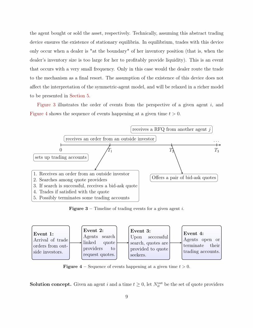
Figure 3 illustrates the order of events from the perspective of a given agent i, and

Figure 4 shows the sequence of events happening at a given time t > 0.

0 T1 T2 T3

sets up trading accounts

receives an order from an outside investor

receives a RFQ from another agent j

. . .

1. Receives an order from an outside investor2. Searches among quote providers3. If search is successful, receives a bid-ask quote4. Trades if satisfied with the quote5. Possibly terminates some trading accounts

Offers a pair of bid-ask quotes

Figure 3 – Timeline of trading events for a given agent i.

Start

Event 1:Arrival of tradeorders from out-side investors.

Event 2:Agents searchlinked quoteproviders torequest quotes.

Event 3:Upon seccessfulsearch, quotes areprovided to quoteseekers.

Event 4:Agents open orterminate theirtrading accounts.

Figure 4 – Sequence of events happening at a given time t > 0.

Solution concept. Given an agent i and a time t ≥ 0, let Noutit be the set of quote providers

9

of agent i at time t, and N init be the set of agents who have i as a quote provider. The sets

(Nit)t≥0 =(Noutit , N in

it

)t≥0

of potential counterparties of agent i are taken right continuous

with left limits (RCLL) almost surely.8 Let Fit represent the information of agent i up to but

excluding time t. That is, Fit is the σ-algebra generated by the sets (Nis)s<t of all potential

counterparties of agent i up to but excluding time t, her past inventories (xis)s<t, the quotes

(pis)s<t = (bis, ais)s<t she offered, the quotes (pis)s<t she was offered, the identities (jis)s<t

of the associated quote providers, the monetary transactions (Pis)s<t related to trading, the

types (Ois)s<t of outside-investor trade orders, and the desired trade directions (Ris)s<t of

Requests for Quotes from other agents. We can take Ois, Ris ∈ Buy, Sell, NA, with the

obvious meanings for “Buy” and “Sell”. The option “NA” indicates that agent i does not

receive a trade order or a Request for Quote at the given time. The monetary transaction Pit

may be associated with a trade with an outsider, another agent or the abstract mechanism.

(i) A search strategy Si of agent i specifies, for every time t > 0, a search decision Sit ∈

Search, No Search. In addition to the prior information Fit, agent i also observes the

type of her outside order at time t, if there is one. Therefore, Sit must be measurable

with respect to F1it, where F1

it represents the combined information9 of Fit and Oit.

(ii) A quoting strategy pj for agent j specifies, for every t > 0, a price pjt that j would

quote upon receiving a Request for Quote. The quote pjt is measurable with respect

to F2jt, where F2

jt represents the combined information of Fjt, Rjt and Ojt.

(iii) A response strategy ρi for agent i specifies, for every t > 0, a trade decision ρit ∈

Purchase, Sale, Rejection. The response ρit is measurable with respect to F3it, where

F3it represents the combined information of Fit, Oit, Rit, pit, pit and jit.

(iv) Let N be the set of all n agents. An account maintenance strategy Nouti of agent i

specifies, for every t ≥ 0, a set Noutit ⊆ N/i of quote providers to i. The choice Nout

it

8An RCLL function is a function defined on R+ that is right-continuous and has left limits everywhere.RCLL functions are standard in the study of jump processes. Please see, for example, Protter (2005). Here,the process (Nit)t≥0 is taken to be RCLL to be consistent with account maintenance behavior in real life. Italso ensures that the set Nit− of counterparties available at time t is well defined for every t > 0.

9That is, F1it = σ(Fit, Oit).

10

is measurable with respect to F4it, where F4

it represents the combined information of

Fit, Oit, Rit, pit, pit, jit, Pit and xit.

The total net payoff to be achieved by agent i, beginning at time t, is

Uit =

∫ ∞t

e−r(s−t)(−βx2

is −∣∣Nout

is

∣∣ c) ds+ Pis dMis− , (2)

where Mit− is the number of trades that agent i has made up to but excluding time t. The

continuation utility of agent i is given by E(Uit | Fit).

In a perfect Bayesian equilibrium (PBE), each agent maximizes her continuation utility

at each time t ≥ 0, with the conjecture that other agents will follow their equilibrium

strategies. I consider perfect Bayesian equilibria in which each agent’s strategy is Markovian

and stationary. Formally, let Yit be the Markov state variable for agent i at time t. That

is, Yit = (xit, Nit, Oit, Rit, pit, pit, jit, Pit). A strategy σi of agent i is Markovian if σit is

measurable with respect to Yit for every t > 0. Thus, a Markovian strategy σi of agent i can

be written as [fit(Yit)]t>0 for some measurable function fit. A Markovian strategy σi is said

to be stationary if for every t > 0, fit(·) = fi(·) for some measurable function fi.

Given any strategy profile σ, let Gt be the associated trading network at time t ≥ 0.

That is, Gt is a directed network with nodes given by the n agents, with a directed link

from node i to j if and only if agent i has a trading account with agent j at time t. The

network Gt may depend on the realization of random events before time t. If there exists a

deterministic trading network G such that for every t ≥ 0, Gt = G almost surely, then G is

said to be the trading network generated by σ. If σ is a PBE in stationary strategies, then

G is simply said to be an equilibrium trading network of the model.

3 Equilibrium, Core-Periphery Network and Core Size

I show that there exists a family of perfect Bayesian equilibria in stationary strategies that

generates trading networks of the form depicted in Figure 1. The family of equilibria is

indexed by the number of core dealers, varying from 0 to m∗, where m∗ is the maximally

11

sustainable number of dealers. I explicitly characterize the family of equilibria, and determine

the maximally sustainable core size. Proofs are given in Appendix B.

Suppose I is some subset of agents, and J is the complement of I, with |J | = m,

|I| = n −m. Anticipating the equilibrium, I will call the agents in I the non-dealers, and

agents in J the dealers. I consider the following strategy profile: At time 0, each non-dealer

agent i ∈ I opens a trading account with all m dealers in J . The dealers in J set up trading

accounts only with each other. In this candidate equilibrium, the m dealers are thus the

common quote providers to all agents.

Equilibrium spread:

An agent searches among her dealer couterparties whenever she receives an outside order,

and does not search otherwise. I denote this search strategy by S∗. Since quote providers

are not allowed to post stub quotes that exceed the total gain π per trade, a quote seeker

optimally trades given any quote. I denote this response strategy by ρ∗. If a given non-dealer

i ∈ I fails his search, then no trade takes place. The inventory of i is therefore always 0,

because a non-dealer cannot take an outside order into his own inventory.

Dealers’ equilibrium bid-ask quotes are anticipated to be of the form (−P, P ), for some

0 < P < π, so that P is the mid-to-bid spread. Thus, non-dealer i earns a profit of π − P

for every outside order that is followed by a successful search.

Non-dealer i must also decide when to open or terminate trading accounts. I let Φd,P

denote the continuation utility of non-dealer i if i maintains d dealer couterparties, for every

0 ≤ d ≤ m. Because outside orders arrive at the mean rate 2λ, and because the probability

of a successful search among the d dealers is θd, it must be the case that for every 0 ≤ d ≤ m,

Φd,P =2λθd(π − P )− dc

r. (3)

For a given stationary mid-to-bid spread P , the continuation utility Φd,P of a non-dealer is

strictly concave in the number d of dealer counterpaties of the non-dealer. Maintaining and

using more dealer trading accounts incurs higher account maintenance costs, which grow

12

linearly with the number of trading accounts, as captured by the term dc in expression (3).

On the other hand, having more dealer counterparties allows the non-dealer to generate

trading profits at a higher mean frequency. The total expected rate of trade profits, as

captured by 2λθd(π−P ), grow sub-linearly with the number d of dealer counterparties. The

net present value is therefore concave in the number d of dealer counterparties.

The equilibrium spread P must satisfy the following non-dealer’s indifference condition

Φm,P = Φm−1,P . (4)

The indifference condition gives a non-dealer the ability to costlessly discontinue any one of

his m trading accounts, making termination of a trading relationship a credible threat to

dealers should they offer aggressively unfavorable prices. Suppose P is determined by the

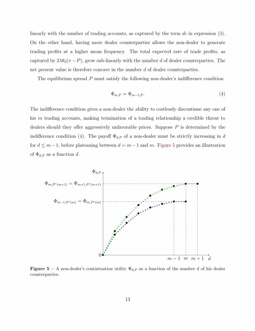
indifference condition (4). The payoff Φd,P of a non-dealer must be strictly increasing in d

for d ≤ m−1, before plateauing between d = m−1 and m. Figure 5 provides an illustration

of Φd,P as a function d.

d0

Φd,P

•

•

•

••

• • •

•

•

•

•

••

• • •

m− 1 m m+ 1

Φm−1,P ∗(m) = Φm,P ∗(m)

Φm,P ∗(m+1) = Φm+1,P ∗(m+1)

Figure 5 – A non-dealer’s contintuation utility Φd,P as a function of the number d of his dealercounterparties.

13

The indifference condition (4) uniquely determines the equilibrium mid-to-bid spread

P ∗(m) = π − c

2λ(θm − θm−1). (5)

I will show that, in equilibrium, an agent’s (dealer or non-dealer) account maintenance

strategy is to always maintain m or m − 1 dealer counterparties, and to discontinue her

trading account with a given dealer whenever the following two conditions are both met:

(i) The agent has m dealer counterparties in total.

(ii) The agent receives an offer price strictly higher than P ∗(m), or a bid price strictly

lower than −P ∗(m).

Whenever these two conditions are met, the agent, after trading with the dealer at the

current price quote, immediately closes her account with the dealer. In particular, any given

dealer always maintains trading accounts with all other m− 1 dealers. I denote this account

maintenance strategy by N∗m. To give an example, suppose non-dealer i wishes to buy 1 unit

of the asset, and dealer j gouges non-dealer i by posting an offer price a that is strictly higher

than the equilibrium offer price P ∗(m). Non-dealer i buys at the price a (since otherwise

i would have lost a profitable opportunity to trade), and then immediately terminates his

trading account with j.

No account termination occurs on the equilibrium path. However, the ability of non-

dealers to terminate their trading accounts constitutes a credible threat to dealers that

would discourage dealers from gouging. I will describe shortly the tradeoff faced by a dealer

when providing price quotes to a non-dealer.

From expression (5) of the equilibrium spread P ∗(m), one obtains the following implica-

tion of dealer price competition.

Proposition 1. The equilibrium mid-to-bid spread P ∗(m) is strictly decreasing in the number

m of dealers. When there is only one dealer, the equilibrium spread P ∗(1) is the monopoly

price that extracts all rents from non-dealers. That is, Φ1,P ∗(1) = 0.

14

If there are more competing dealers in equilibrium, the dealers compete more fiercely for

trades by offering tighter bid-ask quotes. On the other hand, with more competing dealers

in the market, the benefits of serving as a dealer decrease, as each dealer receives a thinner

order flow from non-dealers. This would limit the equilibrium level of dealer competition. I

now demonstrate this intuition, and determine the maximum number m∗ of dealers. I first

describe a quote provider’s optimization problem and derive her optimal quoting strategy.

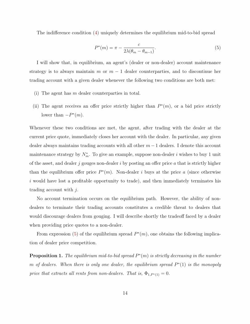
Tightest dealer-sustainable-spread:

I fix some candidate spread P ∈ (0, π], and some number k ≥ 1 of non-dealer customers

of a given dealer j ∈ J . I consider the following continuous-time stochastic control problem

for dealer j, in which j is artificially restricted to the given spread P . (This restriction is

relaxed later.)

Dealer’s problem P(k,m, P ):

• The state space is the set Z of integers, the inventory space of dealer j.

• The control space is −P,−PCB × P, PCB, which is the set of all possible bid-ask

quotes that j may offer. That is, j charges quote seekers the same price P for trading

(either buying or selling) one unit of the asset, and she can make a riskless principal

trade at the price P , with the abstract mechanism assuming the opposite side of the

trade.

• Dealer j receives Requests for Quote from k non-dealers and m− 1 dealers at the total

mean contact rate 2λ(kθm/m+ θm−1). (The “per capita” mean contact rate is 2λθm/m

for non-dealers and 2λθm−1/(m − 1) for dealer customers.) Every contacting agent

seeks to buy or sell 1 unit of the asset, independently across contacts and with equal

probability 1/2.

• The payoff of dealer j is the expected discounted value of all her monetary transfers

and inventory cost, as specified in (2).

15

I denote this problem by P(k,m, P ). In the actual game, a dealer is allowed to post any quote

in [−π, π] rather than being limited to the prices ±P as in the control problem P(k,m, P ).

However, it will be shown that dealers have no incentive to quote prices other than ±P ∗(m),

where P ∗(m) is the equilibrium mid-to-bid spread given by (5). Therefore, the auxiliary

problem P(k,m, P ∗(m)) characterizes an (unrestricted) optimal quoting strategy of a dealer.

I let Vk,m,P be the value function of the dealer in the control problem P(k,m, P ). That

is, Vk,m,P (x) is the maximum attainable continuation utility of the dealer in P(k,m, P ) if her

current inventory is x, for every x ∈ Z. The Bellman principle implies that for every x ∈ Z,

rVk,m,P (x) = −βx2 + λ

(kθmm

+ θm−1

)[Vk,m,P (x+ 1)− Vk,m,P (x) + P ]+

+ λ

(kθmm

+ θm−1

)[Vk,m,P (x− 1)− Vk,m,P (x) + P ]+.

(6)

The first term −βx2 is the inventory flow cost for holding x units of the asset. The sec-

ond term is the expected rate of change in the dealer’s continuation utility associated with

requests to sell. The last term is the analogous mean profit rate from requests to buy. Letting

∆(x) = Vk,m,P (x)− Vk,m,P (x+ 1) (7)

denote the marginal indirect cost from a purchase, one obtains the following lemma:

Lemma 1. Given an inventory level x, the optimal bid and offer prices of the dealer are

b∗(x) =

− P, if ∆(x) ≤ P,

− PCB, if ∆(x) > P,a∗(x) =

P, if ∆(x− 1) ≥ −P,

PCB, if ∆(x− 1) < −P.

That is, the dealer optimally quotes the offer price P whenever her marginal indirect

cost of selling one unit of the asset is lower than the trading benefit P . If the marginal

inventory cost is strictly higher than the benefit P , the dealer is not willing to sell from her

own inventory, resorting to the abstract mechanism to take the other side of the trade.

From the theory of dynamic programming, one can show that the value function Vk,m,P

is even and strictly concave.

16

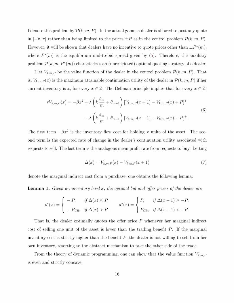
Lemma 2. The function Vk,m,P is even and strictly concave, in that for every x ∈ Z,

Vk,m,P (x) = Vk,m,P (−x), ∆(x) < ∆(x+ 1).

Lemmas 1 and 2 imply that the dealer’s optimal quoting strategy is threshold-type:

Proposition 2. The dealer has a unique optimal quoting strategy [b∗(x), a∗(x)], characterized

by an inventory threshold level xk,m,P ∈ Z:

• If x ≤ −xk,m,P , then [b∗(x), a∗(x)] = [−P, PCB].

• If x ≥ xk,m,P , then [b∗(x), a∗(x)] = [−PCB, P ].

• If −xk,m,P < x < xk,m,P , then [b∗(x), a∗(x)] = [−P, P ].

Proposition 2 indicates that when the dealer is very short (that is, if her inventory is lower

than the threshold −xk,m,P ), she is not willing to sell more assets at the price P , since the

trade gain P no longer covers her marginal inventory cost. Symmetrically, when the dealer’s

inventory size exceeds xk,m,P , she is not willing to buy more. If her inventory is within

the range of (−xk,d,P , xk,d,P ), she is relatively “flat,” and therefore is willing to warehouse

inventory risk.

Now consider whether the dealer has incentive to gouge a non-dealer. If the dealer quotes

some offer price strictly lower than P to an agent requesting to buy, she would have forgone

some trade profit. Similarly, the dealer has no incentive to quote a bid price strictly higher

than −P . If the dealer quotes an offer price strictly higher than P , she increases her trade

profit in the current contact at the cost of possibly losing a non-dealer customer for future

trading. The highest offer price being π, the one-shot incentive by the dealer to gouge is

thus

Π(P ) = π − P. (8)

The case of a quote seeker requesting to sell is symmetric, and gives the dealer the same

one-shot incentive to gouge.

17

The dealer’s future equilibrium profits forgone due to losing one non-dealer customer is

given by the loss in her indirect utility:

Lk,m,P (x) = Vk,m,P (x)− Vk−1,m,P (x). (9)

The dealer has no incentive to deviate from offering the mid-to-bid spread P if and only if

Π(P ) ≤ L(k,m, P ) ≡ k

k +m− 1min

|x|≤xk,m,P

Lk,m,P (x), (10)

where k/(k+m−1) is the probability that the contacting agent is a non-dealer. If inequality

(10) is violated, then there exists some x = −xk,m,P , . . . , xk,m,P such that if the dealer has

a post-trade asset inventory of size x, then gouging by offering the best deviation quote

(−π, π) makes the dealer strictly better off. If (10) holds, then the dealer has no incentive

to gouge on the equilibrium path by the One-Shot Deviation Principle.

A function f : Z→ R is said to be U-shaped if f is even and f(x+ 1) > f(x), ∀x ≥ 0.

Lemma 3. The loss Lk,m,P (x) due to losing one non-dealer customer is U-shaped in x.

Lemma 3 implies that the minimum on the right hand side of (10) is achieved when

x = 0. That is, the dealer has the strongest incentive to gouge when she has no inventory.

When the dealer has a very skewed inventory, she is more reliant on the order flow from her

non-dealer customers to balance her inventory quickly, and thus has less incentive to gouge.

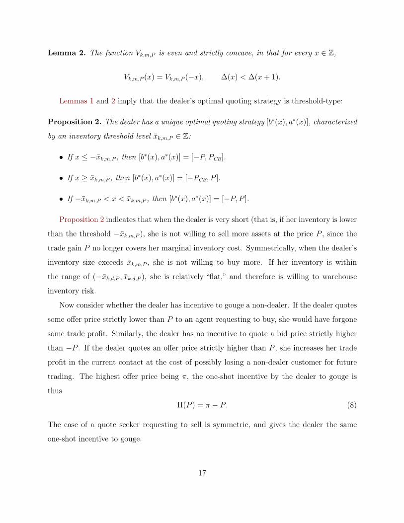
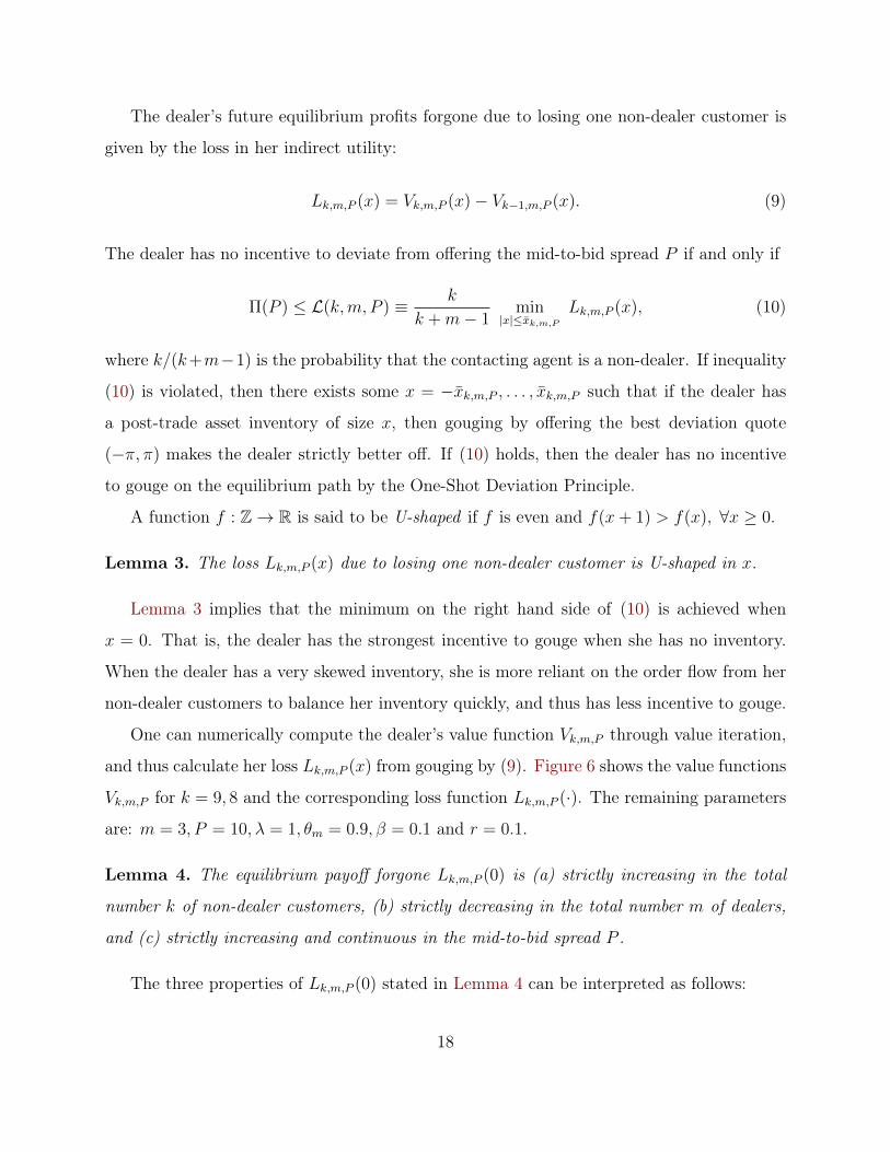
One can numerically compute the dealer’s value function Vk,m,P through value iteration,

and thus calculate her loss Lk,m,P (x) from gouging by (9). Figure 6 shows the value functions

Vk,m,P for k = 9, 8 and the corresponding loss function Lk,m,P (·). The remaining parameters

are: m = 3, P = 10, λ = 1, θm = 0.9, β = 0.1 and r = 0.1.

Lemma 4. The equilibrium payoff forgone Lk,m,P (0) is (a) strictly increasing in the total

number k of non-dealer customers, (b) strictly decreasing in the total number m of dealers,

and (c) strictly increasing and continuous in the mid-to-bid spread P .

The three properties of Lk,m,P (0) stated in Lemma 4 can be interpreted as follows:

18

x-30 -20 -10 0 10 20 30

150

200

250

300

350 Vk,d,P

(x)

Vk-1,d,P

(x)

x-25 -20 -15 -10 -5 0 5 10 15 20 25

39.2

39.25

39.3

39.35

39.4

39.45

39.5

39.55

39.6

39.65

39.7

Lk,d,P

(x)

Figure 6 – The value functions Vk,m,P and Vk−1,m,P , and the loss function Lk,m,P given by (9).

(a) The marginal cost Lk,m,P (0) to the dealer of losing one non-dealer customer can be

broken down into two components: (i) the direct cost of losing the future order flow

from the non-dealer customer, which is partially compensated by (ii) the benefit of

a reduced balance sheet (that is, xk−1,m,P < xk,m,P ) and thus reduced inventory cost.

When the dealer has many non-dealer customers, she is efficient in managing her

inventory by quickly netting many purchases against sales, and thus her inventory cost

is less sensitive to a change in the number of her non-dealer customers (this result about

inventory cost is formulated in Proposition 8). Consequently, the second component

(the benefit of reduced inventory cost) becomes negligible. Hence, losing one non-dealer

customer is more costly to a dealer who has more non-dealer customers.

(b) When the total number m of dealers is larger, each dealer receives a smaller share

of the total order flow from non-dealers. The marginal cost Lk,m,P (0) of losing one

non-dealer customer is thus lower for any given dealer.

(c) If the spread is higher, losing one non-dealer customer is more costly to the dealer.

Given that the one-shot incentive Π(P ) to gouge is strictly decreasing in P , property (c)

of Lemma 4 leads to the following corollary.

19

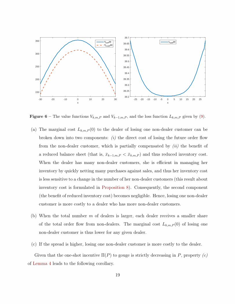
Corollary 1. Condition (10) for not gouging is satisfied if and only if P ≥ P (k,m), where

P (k,m) is uniquely determined by the equality:

Π(P (k,m)) = L(k,m, P (k,m)). (11)

Corollary 1 implies that [−P (k,m), P (k,m)] are the tightest quotes the dealer is willing to

offer without having incentive to deviate. The mid-to-bid spread P (k,m) is called the tightest

(k,m)-dealer-sustainable spread. Any mid-to-bid spread P is (k,m)-dealer-sustainable if and

only if P ≥ P (k,m). Figure 7 illustrates the tradeoff between the gain Π(P ) and the loss

L(k,m, P ) from gouging as P varies, and shows how the tightest dealer-sustainable spread

P (k,m) is determined from the intersection of the two curves.

Π(P )

(k < n−m)

(m′ = n− k > m)

P0

π

P (m) P (k,m) P (m′)

L(n−m,m,P )

L(k,m, P )

L(n−m′,m′, P )

more dealers,less non-dealers

Figure 7 – The tradeoff between the one-shot incentive to gouge and the future profits forgone.

In the actual network trading game, a given dealer has n − m non-dealer customers.

Thus, condition (10) needs to be satisfied for k = n−m for dealers to refrain from gouging.

Letting P (m) ≡ P (n−m,m), P (m) is simply called the tightest m-dealer-sustainable spread.

The next corollary regarding P (k,m) and P (m) follows from (a) and (b) of Lemma 4.

Corollary 2. The tightest (k,m)-dealer-sustainable spread P (k,m) is strictly decreasing in

the number k of non-dealer customers of a given dealer, and the tightest m-dealer-sustainable

spread P (m) is strictly increasing in the number m of dealers.

20

That is, when a dealer has more non-dealer customers, she is able to offer better quotes,

thanks to her ability to efficiently manage inventory risk by more quickly netting purchases

against sales. A well connected dealer is in this sense a liquidity hub. When there are more

dealers in the market, each dealer has reduced efficiency in managing inventory risk, and is

only able to sustain a wider spread. Figure 7 provides an illustration of Corollary 2.

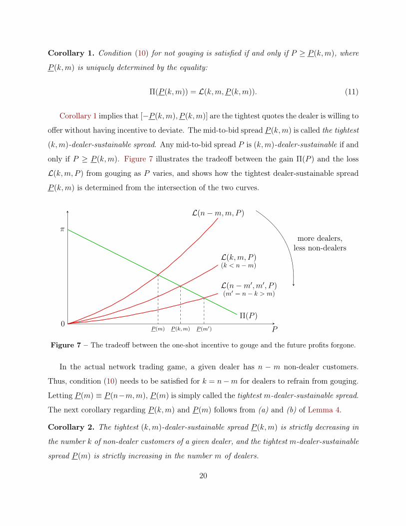
Maximally sustainable core size:

The equilibrium spread P ∗(m), as defined in (5), must be m-dealer-sustainable. Thus,

P ∗(m) ≥ P (m). (12)

Since P ∗(m) is strictly decreasing in m, while P (m) is strictly increasing in m (see Proposi-

tion 1 and Corollary 2), condition (12) is equivalent to

m ≤ m∗, (13)

where m∗ is the largest integer such that

P ∗(m∗) ≥ P (m∗). (14)

The number m∗ is the maximally sustainable core size. Figure 8 illustrates the comparison

between the equilibrium spread P ∗(m) and the tightest sustainable spread P (m) as m varies,

and shows how the maximum core size m∗ is determined from the two spread curves.

Equilibrium existence and uniqueness:

Now I can specify the candidate equilibrium quoting strategy. Suppose a given dealer has

k non-dealer customers (for any k ≤ n−m) at the time she receives a Request for Quote. I

denote the equilibrium bid-ask quote of the dealer by [b∗(x, k), a∗(x, k)].

If P ∗(m) ≥ P (k,m), then

• If −xk,m,P ∗(m) < x < xk,m,P ∗(m), then b∗(x, k) = −P ∗(m), a∗(x, k) = P ∗(m).

21

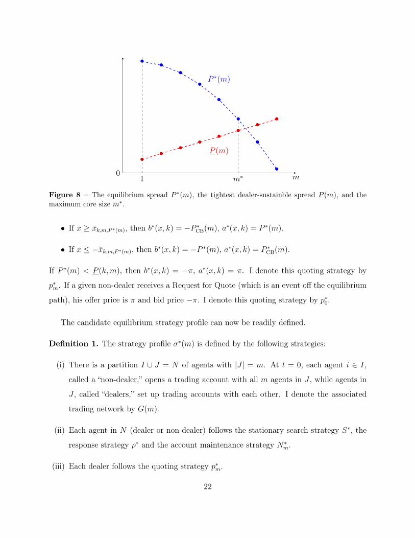
m0

P ∗(m)

P (m)

• ••

•

•

•

•

••

••

••

••

•

1 m∗

Figure 8 – The equilibrium spread P ∗(m), the tightest dealer-sustainble spread P (m), and themaximum core size m∗.

• If x ≥ xk,m,P ∗(m), then b∗(x, k) = −P ∗CB(m), a∗(x, k) = P ∗(m).

• If x ≤ −xk,m,P ∗(m), then b∗(x, k) = −P ∗(m), a∗(x, k) = P ∗CB(m).

If P ∗(m) < P (k,m), then b∗(x, k) = −π, a∗(x, k) = π. I denote this quoting strategy by

p∗m. If a given non-dealer receives a Request for Quote (which is an event off the equilibrium

path), his offer price is π and bid price −π. I denote this quoting strategy by p∗0.

The candidate equilibrium strategy profile can now be readily defined.

Definition 1. The strategy profile σ∗(m) is defined by the following strategies:

(i) There is a partition I ∪ J = N of agents with |J | = m. At t = 0, each agent i ∈ I,

called a “non-dealer,” opens a trading account with all m agents in J , while agents in

J , called “dealers,” set up trading accounts with each other. I denote the associated

trading network by G(m).

(ii) Each agent in N (dealer or non-dealer) follows the stationary search strategy S∗, the

response strategy ρ∗ and the account maintenance strategy N∗m.

(iii) Each dealer follows the quoting strategy p∗m.

22

(iv) Each non-dealer follows the quoting strategy p∗0.

By convention, I denote by σ∗(0) the strategy profile associated with an empty trading

network. That is, no agent opens any account, and no search or trade is conducted.

In the remainder of this section, I fix the model parameters (n, β, π, λ, θ, c, r), and let m∗

be defined as in (14). The first main result of the paper concerns equilibrium existence.

Theorem 1. (a) For every 0 ≤ m ≤ m∗, the strategy profile σ∗(m) is a perfect Bayesian

equilibrium in stationary strategies. (b) For every m > m∗, σ∗(m) is not a PBE.

Theorem 1 shows that there exists a family of perfect Bayesian equilibria in stationary

strategies. Each equilibrium generates a trading network of the form depicted in Figure 1.

The family of equilibria is indexed by the number of core dealers, varying from 0 to m∗,

where m∗ is the maximally sustainable number of dealers. In an equilibrium σ∗(m) for some

0 ≤ m ≤ m∗, the trading network G(m) is stable over time. The equilibrium mid-to-bid

spread is P ∗(m), and dealers are deterred from gouging by the fear of losing non-dealer

customers. Non-dealers do not terminate any account on the equilibrium path, but their

ability to do so constitutes a credible threat that discourages dealers from gouging.

I next provide an equilibrium uniqueness result, stating that P ∗(m) is the unique equi-

librium spread in the equilibrium trading network G(m).

Theorem 2. For every m ≥ 0, if G(m) is the trading network generated by some perfect

Bayesian equilibrium in stationary strategies, then on the equilibrium path, any given dealer

j ∈ J always posts some constant bid price bj and some constant offer price aj, with a spread

equal to bj − aj = 2P ∗(m).

The next theorem follows from Theorems 1 and 2:

Theorem 3. Given some integer m ≥ 0, the network G(m) is the trading network generated

by some perfect Bayesian equilibrium in stationary strategies if and only if 0 ≤ m ≤ m∗.

23

Equilibrium robustness and selection:

The uniqueness of the equilibrium spread P ∗(m) (1 ≤ m ≤ m∗) implies that the equilib-

rium σ∗(m) is robust against dealer collusion:

Corollary 3. Based on any equilibrium σ∗(m) (1 ≤ m ≤ m∗), no collusive price rigging by

any dealer sub-coalition can be sustained by a PBE in stationary strategies.

Even though the uniqueness result of Theorem 2 is sufficient to guarantee no dealer

collusion, it is more intuitive to consider an example of how such a collusion would break

down. If all m dealers were to collude to offer a larger mid-to-bid spread P , then every non-

dealer no longer has incentive to maintain all the m dealer counterparties given the wider

spread. This is because when P > P ∗(m), the non-dealer indifference condition (4) becomes

a strict inequality:

Φm,P < Φm−1,P .

Therefore, any collusion by the m dealers to raise the spread will cause some dealers to

lose some non-dealer customers, destabilizing the trading network. Since losing non-dealer

customers is costly for any given dealer, the dealers cannot credibly engage in such a collusion.

In an equilibrium σ∗(m) of the model (1 ≤ m ≤ m∗), the equilibrium spread P ∗(m)

offered by the m dealers does not compete away all trading profit, as opposed to the case

of Bertrand competition. Imperfect price competition is due to the nature of the sequential

search protocol. Specifically, since agents request quotes sequentially, they cannot screen

price offers simultaneously to select the best one.

On the other hand, dealers charge an equilibrium spread P ∗(m) that is lower than the

monopoly price π, leaving some rent to quote seekers. This is in contrast with the Diamond

paradox, in which all price-setting firms post monopoly prices for consumers who search se-

quentially for price information. In Diamond’s setting, the market is static in that every given

pair of customer and price setting firm meets only once. In this paper, the continuous-time

infinite-horizon trading game features repeated contacts between non-dealers and dealers.

Dealer incentive to widen spread is deterred by the implications for repeated business: a

24

dealer that provides a wider spread increases her trading gain in the current contact, but

non-dealers can credibly cut off the dealer in future trading as a punishment for gouging.

Moreover, the threat of punishment is not only credible, but also renegotiation proof. If a

dealer, after gouging, tries to convince the affected non-dealer to refrain from cutting her off,

the only way she can possibly achieve this goal is by promising the non-dealer a narrower-

than-equilibrium spread in future encounters. However, such a promise is not credible, as it

is common knowledge that the dealer never has incentive to provide a spread that is smaller

than the equilibrium spread P ∗(m).

The idea that repeated business may help circumvent the Diamond paradox also appears

in Bagwell and Ramey (1992), where firms offer a better-than-monopoly price for the fear

of losing customers in future periods. However, Bagwell and Ramey give a continuum of

equilibrium prices, even when the number of firms is fixed. The model of this paper makes

a unique prediction for the equilibrium spread P ∗(m) for a given number m of dealers.

However, Theorem 3 is still not sharp enough, in that it predicts the coexistence of a

family of equilibria indexed by the number of core dealers. The next proposition shows that

these equilibria are Pareto-ranked for non-dealers. This result helps to offer a criterion for

equilibrium selection.

Proposition 3. The equilibrium outcomes induced by the strategy profiles σ∗(m) (0 ≤ m ≤

m∗) are Pareto-ranked for non-dealers, in that every non-dealer enjoys a strictly higher payoff

under σ∗(m′) than σ∗(m), for any 0 ≤ m < m′ ≤ m∗.

Proposition 3 suggests that all non-dealers prefer an equilibrium with more competing

dealers, since the benefit associated with a tighter equilibrium spread and more frequent

trading outweighs additional account maintenance costs. A graphical illustration of Propo-

sition 3 is provided by Figure 5. One implication of Proposition 3 is equilibrium selection: an

equilibrium σ(m) with fewer core dealers may be ruled out if agents can actively coordinate

the selection of dealers. To see this, suppose σ∗(m′) is an equilibrium with more core dealers

m′ > m. Any m′ − m non-dealers under the equilibrium σ∗(m) can credibly propose to

serve as core dealers, on top of the existing m dealers, as such a proposal will result in a

25

new equilibrium σ∗(m′). The m′ −m newly entered dealers improve their payoff by exploit-

ing their central network position to earn intermediation spread Following Proposition 3,

the remaining n−m′ non-dealers also benefit from greater dealer competition. Finally, the

m existing dealers lose some of the market, and are forced to provide a narrower spread

P ∗(m′) < P ∗(m). However, they have no choice other than adapting to their new equi-

librium strategies, as an existing dealer who refuses to lower her spread risks losing future

business and ultimately her dealer position.

The equilibrium σ∗(m∗) with the maximum number of core dealers cannot be overturned

in this manner, since non-dealers cannot credibly propose to enter as additional dealers.

Therefore, the equilibrium σ∗(m∗) is uniquely robust against dealer entry. This selection

procedure through dealer entry can be regarded as a form of price competition, since non-

dealers can enter as dealers to compete for trades. Here, the non-dealers are able to com-

municate their intention to serve as dealers, even though they are unable to commit to a

tighter spread level. The selection procedure closely mimics the logic of coalition-proof Nash

equilibrium introduced by Bernheim, Peleg, and Whinston (1987). In the family of equilibria

[σ∗(m)]0≤m≤m∗ , the only coalition-proof equilibrium is σ∗(m∗).

The discussion above is summarized in the following proposition:

Proposition 4. The equilibrium σ∗(m∗) is the unique equilibrium in the family [σ∗(m)]0≤m≤m∗

that is robust against dealer entry.

Alternative core-periphery structures:

Thus far, I have considered equilibria that generate a trading network of the form de-

picted in Figure 1. Alternative network structures have not been examined yet. In practice,

observed core-periphery structures in OTC markets are less “concentrated,” in that a typical

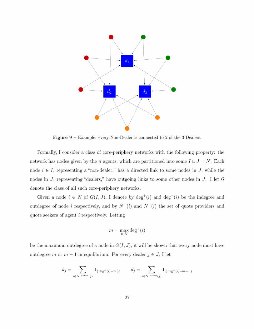
non-dealer is connected to some dealers, but not to all of them. Figure 9 illustrates such an

example of core-periphery structure. I next turn to whether such a trading network could

emerge in equilibrium, and if so, how many dealers could reside in the core, and how many

trading accounts a non-dealer would have.

26

d1

d2 d3

Figure 9 – Example: every Non-Dealer is connected to 2 of the 3 Dealers.

Formally, I consider a class of core-periphery networks with the following property: the

network has nodes given by the n agents, which are partitioned into some I ∪ J = N . Each

node i ∈ I, representing a “non-dealer,” has a directed link to some nodes in J , while the

nodes in J , representing “dealers,” have outgoing links to some other nodes in J . I let G

denote the class of all such core-periphery networks.

Given a node i ∈ N of G(I, J), I denote by deg+(i) and deg−(i) be the indegree and

outdegree of node i respectively, and by N+(i) and N−(i) the set of quote providers and

quote seekers of agent i respectively. Letting

m = maxi∈N

deg+(i)

be the maximum outdegree of a node in G(I, J), it will be shown that every node must have

outdegree m or m− 1 in equilibrium. For every dealer j ∈ J , I let

kj =∑

i∈Ntextin(j)

1deg+(i)=m , dj =∑

i∈Ntextin(j)

1deg+(i)=m−1

27

be the number of quote seekers of j that have outdegree m and m− 1 respectively. Only the

quote seekers with outdegree m can costlessly terminate their trading accounts with j. I let

Vk,m,d,P be the value function that solves the following HJB equations: for every x ∈ Z,

rVk,m,d,P (x) = −βx2 + λ

(kθmm

+ dθm−1

m− 1

)[Vk,m,d,P (x+ 1)− Vk,m,d,P (x) + P ]+

+ λ

(kθmm

+ dθm−1

m− 1

)[Vk,m,d,P (x− 1)− Vk,m,d,P (x) + P ]+.

I let Lk,m,d,P be the loss in the indirect utility function associated with losing one quote

seeker:

Lk,m,d,P = Vk,m,d,P − Vk−1,m,d,P .

Similar to Lemma 3, one can show that Lk,m,d,P is U-shaped. I let

L(k,m, d, P ) =k

k + dLk,m,d,P (0).

and P (k,m, d) ∈ R+ be determined by the equality

Π(P (k,m, d)) = L(k,m, d, P (k,m, d)).

Similar to Corollary 2, one can show that P (k,m, d) is strictly decreasing in k. I letk(m, d)

be the smallest integer such that

P (k(m, d),m, d) ≤ P ∗(m),

where P ∗(m) is the equilibrium spread as given by expression (5). Any given dealer j ∈ J

needs at least k(m, dj) quote seekers to sustain the equilibrium spread P ∗(m) without having

incentive to gouge. The following theorem generalizes Theorem 3 by providing a necessary

and sufficient condition for G(I, J) to be an equilibrium network.

Theorem 4. The core-periphery network G(I, J) is the equilibrium network generated by

some perfect Bayesian equilibrium in stationary strategies if and only if (i) every node has

outdegree m or m− 1, and (ii) for every dealer j ∈ J , kj ≥ k(m, dj).

28

Since P (k,m, d) is strictly increasing in m, I define m∗ to be the largest integer such that

P ∗(m∗) ≥ mink+d=n−1

P (k, m∗, d).

Then in order for all dealers to have no incentive to gouge, any agent has at most m∗ dealer

counterparties. By the same equilibrium selection procedure through dealer entry following

Proposition 3, one can focus on the case of maximum dealer competition m = m∗. It follows

from Theorem 4 that the total number of dealers is bounded above.

Corollary 4. If a core-periphery network G(I, J) ∈ G is an equilibrium network generated by

some perfect Bayesian equilibrium in stationary strategies, then the total number of dealers

is bounded by

|J | ≤ m∗n

k(m∗, 0)− 1.

To provide a numerical example, I consider a market with n = 1000 agents, with β =

0.1, π = 1, λ = 3, θd = 1 − 0.8d, c = 0.09, and r = 0.1. In equilibrium, every non-dealer

has m∗ = 3 trading accounts, the equilibrium spread is P ∗(m∗) ' 0.1, every dealer needs to

have at least k(m∗, 0) = 166 non-dealer customers, and the upper bound on the number of

dealers is |J | ≤ 17.

4 Comparative Statics, Welfare and Policy Implications

To develop comparative statics on the core size, I focus attention on the equilibrium σ∗(m∗)

that generates the core-periphery network G(m∗) with m∗ dealers, as depicted in Figure 1.

The core size m∗ and the equilibrium spread P ∗(m∗):

The next proposition shows how the core size varies as a function of the model parameters

(n, β, π, λ, θ, c, r). I will fix all but one parameter and examine how the core size m∗, as

defined in (14), is affected by the remaining parameter. Proofs are given in Appendix C.

Proposition 5. (i) The core size m∗ is weakly increasing in the total number n of agents.

29

(ii) For n sufficiently large, the core size reaches a constant m∗∞ that is independent of n.

The constant m∗∞ is the largest integer m such that

mrπ

2λθm +mr< P ∗(m).

(iii) The core size m∗ is weakly increasing in the total gain per trade π and the arrival

rate λ of trade orders from outside investors, and weakly decreasing in the account

maintenance cost c and the inventory risk coefficient β.

(iv) The equilibrium spread P ∗(m∗) is weakly increasing in the inventory risk coefficient β,

and weakly decreasing in the total number n of agents.

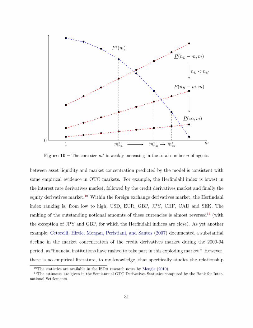
Part (i) of Proposition 5 has a simple intuitive proof, as follows. Suppose there are

m dealers in the market. As the total number n of agents increases, each dealer becomes

more efficient in inventory management, and thus can support a tighter spread P (n−m,m).

That the dealer-sustainable spread P (n−m,m) is strictly decreasing in n is a consequence

of Corollary 2. In contrast, the equilibrium spread P (m) does not depend on n. The core

size m∗, which is the largest integer such that the P (m∗) ≥ P (n −m∗,m∗), is thus weakly

increasing in n. Figure 10 provides a graphical illustration of this result.

Part (ii) says that even for an “infinite” set of investors, one should anticipate only a finite

number m∗∞ of dealers. A proof is given in Appendix B. To provide a numerical example of

the numberm∗∞ of dealers in a large market, let π = 1, λ = 3, θd = 1−0.8d, c = 0.09, s = 0.1,

and r = 0.1. Thenm∗∞ = 3, and the equilibrium spread in the large market is P ∗(m∗∞) ' 0.1.

As π increases, dealers extract a higher rent per trade (reflected by a wider equilibrium

spread P ∗(m)), but also have stronger incentive to gouge (wider dealer-sustainable spread

P (m)). It will be shown, in Appendix B, that the equilibrium spread P ∗(m) increases more

than the dealer-sustainable spread P (m). The core size m∗ is thus weakly increasing in π.

The parameter λ can be interpreted as a measure of asset liquidity, since it is the rate

at which the economy wishes to trade the asset. With a more liquid asset, it is natural that

more dealers emerge to facilitate the intermediation of the asset. The negative relationship

30

m0

P ∗(m)

P (nH −m,m)

P (nL −m,m)

P (∞,m)

nL < nH

••

•

•

•

•

•

•• • • • • • • ••

••

••

••

•

•

•

•

•

•

•

•

•

1 m∗nLm∗nH

m∗∞

Figure 10 – The core size m∗ is weakly increasing in the total number n of agents.

between asset liquidity and market concentration predicted by the model is consistent with

some empirical evidence in OTC markets. For example, the Herfindahl index is lowest in

the interest rate derivatives market, followed by the credit derivatives market and finally the

equity derivatives market.10 Within the foreign exchange derivatives market, the Herfindahl

index ranking is, from low to high, USD, EUR, GBP, JPY, CHF, CAD and SEK. The

ranking of the outstanding notional amounts of these currencies is almost reversed11 (with

the exception of JPY and GBP, for which the Herfindahl indices are close). As yet another

example, Cetorelli, Hirtle, Morgan, Peristiani, and Santos (2007) documented a substantial

decline in the market concentration of the credit derivatives market during the 2000-04

period, as “financial institutions have rushed to take part in this exploding market.” However,

there is no empirical literature, to my knowledge, that specifically studies the relationship10The statistics are available in the ISDA research notes by Mengle (2010).11The estimates are given in the Semiannual OTC Derivatives Statistics computed by the Bank for Inter-

national Settlements.

31

between asset liquidity and market concentration.

If dealers become less risk tolerant (higher β), they find it more costly to use their own

inventories to make markets. As a result, dealers need to be compensated with a wider

spread P (m) to continue making a two-way market. On the other hand, the equilibrium

spread P ∗(m) is not affected by dealer risk tolerance, as it is determined by an indifference

condition for non-dealers. Therefore, the market can only support a smaller core with agents

of reduced risk tolerance.

A current hotly debated issue is bond market liquidity. The world’s biggest banks are

shrinking their bond trading activities to comply with regulations such as the Volcker rule

and higher capital requirements imposed after the financial crisis. These restrictions have

curbed the ability of banks to build inventory or warehouse risk. On Friday, October 23,

2015, Credit Suisse exited its role as a primary dealer across Europe’s bond markets, the

latest signal that banks are scaling back bond trading activities. There are also other ex-

amples of markets, such as corporate bond markets and currency markets, which are slowly

experiencing structural changes due to significant dealer disintermediation. Intermediation

in these markets is increasingly agency-based, and many investors report that post-crisis

regulatory reforms have reduced market liquidity.

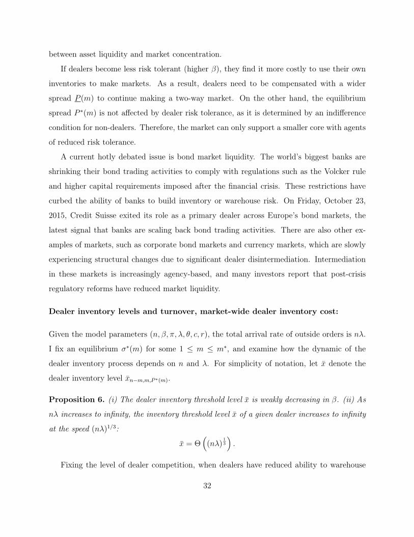
Dealer inventory levels and turnover, market-wide dealer inventory cost:

Given the model parameters (n, β, π, λ, θ, c, r), the total arrival rate of outside orders is nλ.

I fix an equilibrium σ∗(m) for some 1 ≤ m ≤ m∗, and examine how the dynamic of the

dealer inventory process depends on n and λ. For simplicity of notation, let x denote the

dealer inventory level xn−m,m,P ∗(m).

Proposition 6. (i) The dealer inventory threshold level x is weakly decreasing in β. (ii) As

nλ increases to infinity, the inventory threshold level x of a given dealer increases to infinity

at the speed (nλ)1/3:

x = Θ(

(nλ)13

).

Fixing the level of dealer competition, when dealers have reduced ability to warehouse

32

risk, they optimally shrink their balance sheet to control inventory risk. When the asset is

more liquid (either because of a larger rate λ or because of a larger market), dealers expand

their inventory size to take advantage of the increased order flow from quote seekers.

The inventory process (xjt)t≥0 of a given dealer j is a symmetric continuous-time random

walk on −x, . . . , x, with jump intensity ϑ (the total rate of Requests for Quote received by

dealer j). The random walk xjt loops at the boundary points ±x. Therefore, the inventory

process has a unique stationary distribution that is the uniform distribution on its set of

states. It is well known that the mixing time of this process is on the order of x2/ϑ as ϑ goes

to infinity.12 Therefore, one has the following proposition:

Proposition 7. As nλ goes to infinity, the mixing time tmix of the inventory process (xjt)t≥0

of a dealer is on the order of (nλ)−1/3:

tmix = Θ(

(nλ)−13

).

The proposition above implies that in a liquid asset market, dealer inventory has quick

turnover and exhibits fast mixing. The positive relationship between asset liquidity and the

speed of dealer inventory rebalancing, as predicted by the model, is consistent with prior em-

pirical studies. Using data on the actual daily U.S.-dollar inventory held by a major dealer,

Duffie (2012) estimates that the “expected half-life” of inventory imbalances is approximately

3 days for the common shares of Apple, versus two weeks for a particular investment-grade

corporate bond. The data also reveal substantial cross-sectional heterogeneity across indi-

vidual equities handled by the same market maker, with the expected half-life of inventory

imbalances being the highest for (least liquid) stocks with the highest-bid-ask spreads and

the lowest trading volume.

The payoff Vn−m,m,P (0) of a dealer can be decomposed into her inventory cost and her12Examples 5.3.1, 12.10 and Theorem 20.3 of Levin, Peres, and Wilmer (2009) provide background on the

mixing time of this process.

33

gain from trading with quote seekers:

Vn−m,m,P (0) = −C(n, λ,m) + 2λ

((n−m)

θmm

+ θm−1

)︸ ︷︷ ︸

:=ϑ, total rate of Requests for Quote

P

r. (15)

For a given dealer, the total rate ϑ of Requests for Quote and thus the total trade gain grow

linearly with n and λ. The inventory cost C(n, λ,m), as shown by the next proposition,

grows sublinearly with n and λ.

Proposition 8. (i) The present value C(n, λ,m) of individual dealer inventory cost is strictly

increasing and strictly concave in n and λ. (ii) As nλ increases to infinity, the inventory

cost C(n, λ,m) goes to infinity at the speed (nλ)2/3:

C(n, λ,m) = Θ(

(nλ)23

).

(iii) The market-wide total dealer inventory cost mC(n,m, λ) is strictly increasing in m.

In the model setup, every agent has a quadratic inventory holding cost βx2. However, as

the total rate of Requests for Quote increases, a given dealer is more efficient in balancing

her inventory by quickly netting trades. The netting effect more than offsets the convexity

of the inventory cost function. Indeed, property (i) of Proposition 8 probably holds for any

convex inventory cost function f(x): if the cost f(x) increases very fast with the inventory

size |x|, the dealer would optimally reduce her inventory level to control her inventory cost.

Property (iii) follows from the decreasing returns to scale of the individual inventory cost

function C(n,m, λ) and Jensen’s inequality. To minimize the market-wide dealer inventory

cost, it is better to concentrate the provision of immediacy at a smaller set of dealers in

order to maximize the netting efficiency.

Welfare analysis and policy discussion:

From the viewpoint of market efficiency, dealers tend to under-compete in liquid markets,

and over-compete in illiquid markets. The next proposition establishes this welfare result,

which suggests regulation policies on market makers that are differentiated by asset liquidity.

34

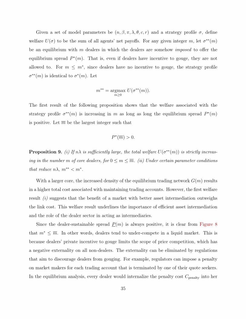
Given a set of model parameters be (n, β, π, λ, θ, c, r) and a strategy profile σ, define

welfare U(σ) to be the sum of all agents’ net payoffs. For any given integer m, let σ∗∗(m)

be an equilibrium with m dealers in which the dealers are somehow imposed to offer the

equilibrium spread P ∗(m). That is, even if dealers have incentive to gouge, they are not

allowed to. For m ≤ m∗, since dealers have no incentive to gouge, the strategy profile

σ∗∗(m) is identical to σ∗(m). Let

m∗∗ = argmaxm≥0

U(σ∗∗(m)).

The first result of the following proposition shows that the welfare associated with the

strategy profile σ∗∗(m) is increasing in m as long as long the equilibrium spread P ∗(m)

is positive. Let m be the largest integer such that

P ∗(m) > 0.

Proposition 9. (i) If nλ is sufficiently large, the total welfare U(σ∗∗(m)) is strictly increas-

ing in the number m of core dealers, for 0 ≤ m ≤ m. (ii) Under certain parameter conditions

that reduce nλ, m∗∗ < m∗.

With a larger core, the increased density of the equilibrium trading network G(m) results

in a higher total cost associated with maintaining trading accounts. However, the first welfare

result (i) suggests that the benefit of a market with better asset intermediation outweighs

the link cost. This welfare result underlines the importance of efficient asset intermediation

and the role of the dealer sector in acting as intermediaries.

Since the dealer-sustainable spread P (m) is always positive, it is clear from Figure 8

that m∗ ≤ m. In other words, dealers tend to under-compete in a liquid market. This is

because dealers’ private incentive to gouge limits the scope of price competition, which has

a negative externality on all non-dealers. The externality can be eliminated by regulations

that aim to discourage dealers from gouging. For example, regulators can impose a penalty

on market makers for each trading account that is terminated by one of their quote seekers.

In the equilibrium analysis, every dealer would internalize the penalty cost Cpenalty into her

35

loss function L(n − m,m,P ) from gouging, and can thus sustain a tighter spread P (m).

Such a penalty cost on dealers, surprisingly, encourages dealer entry. This is because the

penalty creates room for greater dealer competition by improving the commitment power

of a dealer. By choosing an appropriate cost value Cpenalty, the regulator can achieve the

socially optimal level of market concentration. Figure 11 provides a graphical illustration of

the effect of such a penalty cost Cpenalty.

Π(P )

P0

π

P (m) P (m)

L(n−m,m,P ) + Cpenalty

L(n−m,m,P )

m0

P ∗(m)

P (m)

P (m)

• • •••

•

•

•• • • • • • • •

••••••••

1 m∗ m

Figure 11 – Introducing a penalty cost Cpenalty on gouging increases dealer competition.

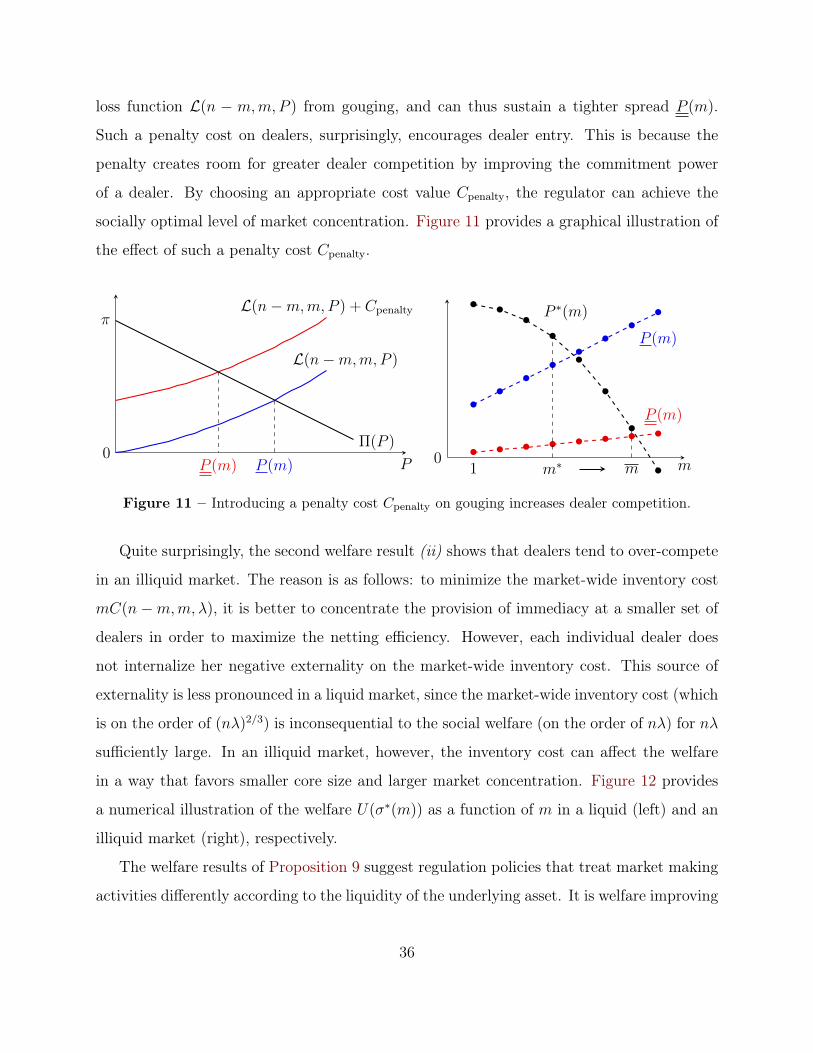
Quite surprisingly, the second welfare result (ii) shows that dealers tend to over-compete

in an illiquid market. The reason is as follows: to minimize the market-wide inventory cost

mC(n−m,m, λ), it is better to concentrate the provision of immediacy at a smaller set of

dealers in order to maximize the netting efficiency. However, each individual dealer does

not internalize her negative externality on the market-wide inventory cost. This source of

externality is less pronounced in a liquid market, since the market-wide inventory cost (which

is on the order of (nλ)2/3) is inconsequential to the social welfare (on the order of nλ) for nλ

sufficiently large. In an illiquid market, however, the inventory cost can affect the welfare

in a way that favors smaller core size and larger market concentration. Figure 12 provides

a numerical illustration of the welfare U(σ∗(m)) as a function of m in a liquid (left) and an

illiquid market (right), respectively.

The welfare results of Proposition 9 suggest regulation policies that treat market making

activities differently according to the liquidity of the underlying asset. It is welfare improving

36

m0 5 10 15

×1010

0

1

2

3

4

5

6

U(σ *(m))

m1 2 3 4 5 6 7 8 9

×104

4

5

6

7

8

9

10

U(σ *(m))

Figure 12 – The welfare U(σ∗(m)) for m = 1, 2, . . . ,m∗.

to encourage dealer participation in liquid markets, and discourage such in illiquid ones. The

current regulatory capital requirement adopted by Basel III uses risk-weighted assets as the

denominator of the capital ratio of a bank. This approach can be improved, for example, by

adding a liquidity component in the weight calculation.

Of course, excessive risk taking by dealers increases their probability of default. One

of the main reasons for regulators to introduce the Volcker rule and more stringent capital

requirements is to discipline dealers’ risk taking behavior, in order to reduce their default risk

and mitigate the impact of a dealer default on the rest of the market. However, these policies

may also have a long term impact on market structure and adversely affect market liquidity.

These consequences should not be ignored. This paper does not consider dealer default

risk or contagion risk in the financial network, and therefore Propositions 5 and 9 are not

sufficient to provide a complete policy assessment for the Volcker rule or capital requirements.

However, it offers an analytic framework from the perspective of intermediation efficiency,

and identifies two sources of externalities related to dealer competition for the analysis of

these regulation policies on market makers.

Non-bank firms such as fund managers are holding more bonds and starting to act as

liquidity providers in daily trading. However, many question whether these buy-side firms

37

can substitute for dealer liquidity by taking an effective role as market makers. The model

outlined in this paper highlights the importance of having a large customer base for an agent

to efficiently manage inventory and make markets. Non-bank firms such as fund managers

are not naturally liquidity hubs. They do not have the same number of trading lines and

global customer base that banks have. Being in a central network position is essential for a

financial institution to be able to “lean against the wind” — that is, to provide liquidity during

financial disruptions. It is worrisome that the liquidity that non-bank firms are providing

may be “illusory”: these firms may be unable or unwilling to absorb external selling pressure

in a selloff, and liquidity may vanish. However, this paper does not cover this topic. A

different model is needed to illustrate liquidity illusion.

5 Inter-Dealer Trading through Nash Bargaining

In practice, dealers form a completely connected core and trade with each other actively

to share their inventory risk accumulated when trading with non-dealers. The protocol for

bilateral inter-dealer trading usually features Nash bargaining of some sort, rather than a

request-for-quote by one counterparty and a take-it-or-leave-it offer by the other. When

dealers are allowed to trade larger quantities with each other at a bilaterally negotiated

price, they are able to extract gains from trade more efficiently. In this section, I illustrate

this intuition through a variant of the symmetric-agent model, in which dealers are allowed

to conduct Nash Bargaining when trading with each other. The model no longer preserves

agent symmetry, as a subset of agents (dealers) have access to a trading protocol featuring

Nash bargaining that is not available to other agents (non-dealers). In practice, dealers

resist the participation of non-dealers into the inter-dealer segment, and accuse non-dealers

of taking liquidity without exposing themselves to the risks of providing liquidity. Others

criticize dealers for trying to prevent competition that would compress bid-ask spreads in

the market.

The structure of the trading game to be considered is similar to that of the symmetric-

agent model. A common non-divisible asset with 0 expected payments is traded over the

38

counter by n agents. Every agent has 0 initial endowment of the asset, and is subject to an

instantaneous quadratic inventory cost of −βx2 when holding an asset inventory of size x.

The time discount rate is r. The total present value of a given agent is given by (2). Every

agent serves outside investors, who submit trade orders at the mean arrival rate 2λ and pay

a fixed premium π > 0, as described in the symmetric-agent model of Section 2. At time

t = 0, agents open trading accounts, which are subject to termination at any time t > 0.

The cost of maintaining an account is c per unit of time.

All model assumptions made so far are identical to the symmetric-agent model. I next

introduce agent asymmetry. There is a partition of agents I ∪ J = N with J = m. Agents

in J , called “dealers,” give each other Nash bargaining rights. Specifically, if a pair of dealers

j1, j2 ∈ J have trading accounts with each other, they can bilaterally negotiate the terms of

trade according to Nash bargaining when they meet. In the current context of spot trading,

terms of trade simply consist of price and quantity. Agents in I, called “non-dealers,” have no

access to this inter-dealer trading protocol. That is, even if a non-dealer i ∈ I and another

agent (dealer or non-dealer) have trading accounts with each other, the pair can only trade

following the request-for-quote protocol upon contact.

The search technology also differs between dealer-to-dealer and dealer-to-non-dealer en-

counters. The probability of a successful search among d dealers is given by θd, where

θd ∈ [0, 1) is strictly increasing and strictly concave in d, with θ(0) = 0. This is the same

search technology in the symmetric-agent model. Encounters between pairs of dealers are

based on independent random matching, with pair-wise meeting intensity ζ.

The information structure is largely identical to that of the symmetric-agent model.

In particular, the model maintains quote offer privacy and inventory privacy for trading

between dealers and non-dealers. However, there are two differences: (i) the assumption of

quote seeker anonymity is relaxed. That is, when a non-dealer requests quotes from another

agent (dealer or non-dealer), the identity of the quote seeker is revealed to the quote provider.

(ii) When two dealers meet, they observe each others’ inventory in order to conduct Nash

bargaining. It would be desirable to maintain inventory privacy for all agents. However,

bargaining with incomplete information is a notoriously hard problem in the literature of

39

economics. I do not explore this direction, and instead assume complete information when

it comes to inter-dealer bargaining, so that the paper maintains focus on core-periphery

network formation and trading.

The same solution concept of perfect Bayesian equilibrium in stationary strategies, as

defined in Section 2, is applied to this network trading game. I focus on large markets

when solving this model. This restriction is not necessary when solving the symmetric-agent

model.

Formally, consider a core-periphery network defined as follows: The network has nodes

given by the n agents, which are partitioned into some I ∪ J = N with |J | = m for some

0 ≤ m ≤ n. Each node i ∈ I, representing a “non-dealer,” has a directed link to all the m

nodes in J , while each node j ∈ J , representing a “dealer,” has a bidirectional link with all

other m− 1 nodes in J . I let Gn(m) denote such a network.

Theorem 5. For a given set of model parameters (n,m, β, π, λ, θ, c, r), suppose m∗ is defined

as in (14). There is some constant n0, such that if n > n0, the following is true: given some

integer m ≥ 0, the network Gn(m) is the equilibrium trading network generated by some

symmetric perfect Bayesian equilibrium in stationary strategies if and only if 0 ≤ m ≤ m∗.

6 Concluding Remarks

Extensive empirical work has shown that core-periphery networks dominate conventional

OTC markets. However, few (though an increasing number of) theoretical foundations

have been provided. Existing literature exploits some ex-ante heterogeneity of agents to

explain the ex-post difference of their network positions. The symmetric-agent model of

this paper is original in its ability to provide a separation of core from periphery agents

that is determined solely by endogenous forces that tend to concentrate the provision of

immediacy. The equilibrium level of dealer entry (the size of the core) depends on the

combined effect of two countervailing forces: (i) network competition among dealers in their

pricing of immediacy to peripheral agents, and (ii) the benefits of a concentrated set of

dealers for lowering inventory risk through their ability to quickly offset purchases and sales.

40

Although financial institutions do not have identical characteristics in real OTC markets,

the equilibrium results implied by the symmetric-agent model highlight the important role

of these two economic forces in the formation of market structure.

One useful direction of future research would be the introduction of agent heterogeneity

to study the relationship between dealer centrality and the pricing of immediacy. Recent em-

pirical work suggests that the price-centrality relationship changes across different markets.

In the municipal bond market, central intermediaries earn higher markups compared with

peripheral intermediaries.13 The opposite is true in the market for asset-backed securities.14

Another feature of the model is that dealer profits only come from earning bid-ask spread

through frequent intermediation of the asset, and not from their idiosyncratic taste for the as-

set. This echoes the finding by Farboodi, Jarosh, and Shimer (2015) that fast intermediation

dampens the effect of idiosyncratic taste on a dealer’s net valuation of the asset.

From a welfare viewpoint, the model identifies two sources of externalities: (1) dealers’

private incentive to gouge, which limits the scope of price competition, and (2) the negative

externality of each individual dealer on the overall netting efficiency. The first externatlity

dominates in a liquid market, and leads to insufficient dealer competition. Introducing

an additional penalty cost on market makers for “each lost customer” deters dealers from

gouging, improves their commitment power, and therefore creates room for greater dealer

competition. The second externality is more pronounced in an illiquid market, and results

in a higher than socially optimal level of dealer competition. The model suggests regulation

policies that treat market makers differently according to asset liquidity through, for example,

the introduction of a “liquidity weight,” on top of the currently used “risk weight.”

13Li and Schürhoff (2014) provide evidence for the municipal bond market.14See Hollifield, Neklyudov, and Spatt (2014) provide evidence for the market of asset-backed securities.

41

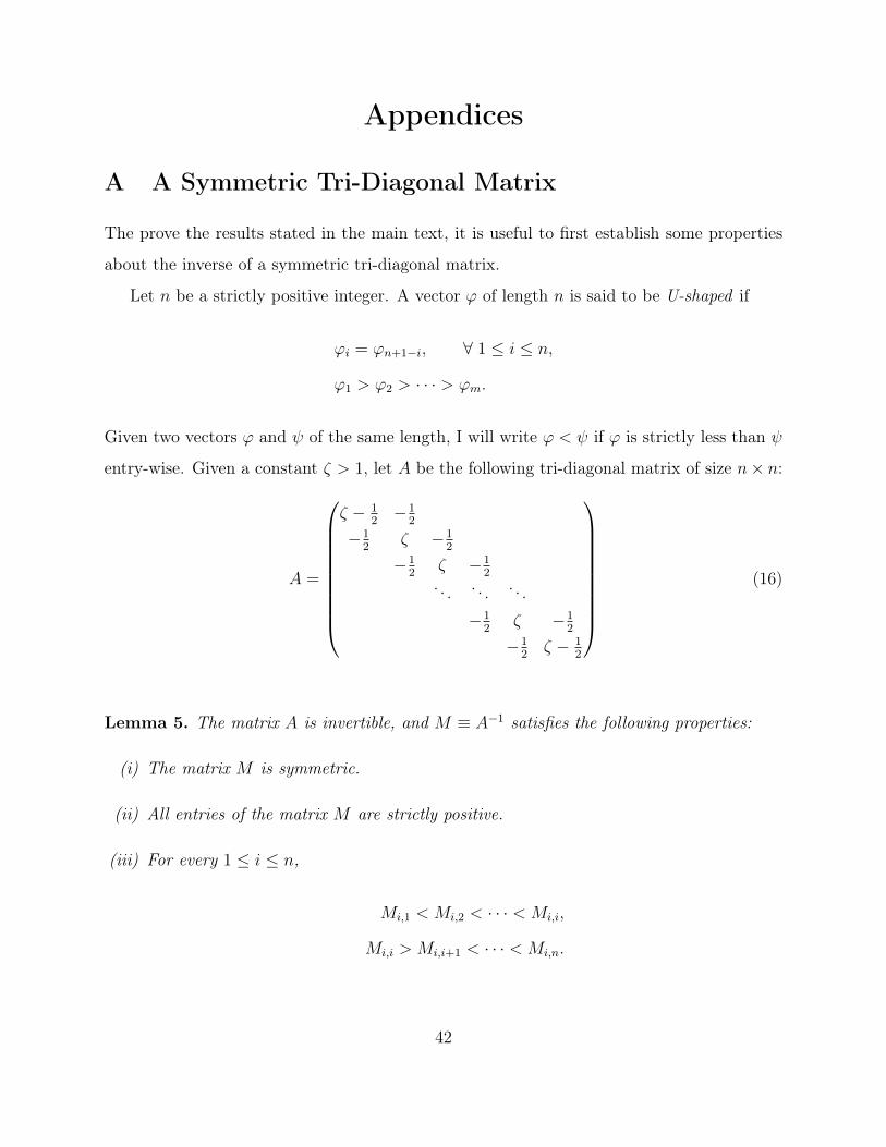
Appendices

A A Symmetric Tri-Diagonal Matrix

The prove the results stated in the main text, it is useful to first establish some properties

about the inverse of a symmetric tri-diagonal matrix.

Let n be a strictly positive integer. A vector ϕ of length n is said to be U-shaped if

ϕi = ϕn+1−i, ∀ 1 ≤ i ≤ n,

ϕ1 > ϕ2 > · · · > ϕm.

Given two vectors ϕ and ψ of the same length, I will write ϕ < ψ if ϕ is strictly less than ψ

entry-wise. Given a constant ζ > 1, let A be the following tri-diagonal matrix of size n× n:

A =

ζ − 12−1

2

−12

ζ −12

−12

ζ −12

. . . . . . . . .

−12

ζ −12

−12

ζ − 12

(16)

Lemma 5. The matrix A is invertible, and M ≡ A−1 satisfies the following properties:

(i) The matrix M is symmetric.

(ii) All entries of the matrix M are strictly positive.

(iii) For every 1 ≤ i ≤ n,

Mi,1 < Mi,2 < · · · < Mi,i,

Mi,i > Mi,i+1 < · · · < Mi,n.

42

(iv) For every i 6= j,

Mi,j−1 +Mi,j+1 > 2Mi,j.

(v) For every i, j, Mi,j = Mn+1−i,n+1−j.

(vi) For every vector y that is U-shaped, My is U-shaped and (My)n ≤ yn/(ζ − 1).

(vii) Let m = b(n+ 1)/2c. For every i ≤ m, M2i,1 ≥M2

n+1−i,1 and

M2m,1 −M2

n+1−m,1 <2

ζ − 1.

Proof. Since ζ > 1, the matrix A is diagonally dominant thus invertible. Its inverse M is

symmetric since A is. The matrix A can be written as A = cI −B/2, where

B =

1 1

1 1

1 1. . . . . .

1 1

1 1

(17)

The sup-norm of the matrix B is ||B||∞ = 2. Since ζ > 1, one can write the following

expansion for M :

M = A−1 = ζ−1

(I − B

2ζ

)−1

= ζ−1

[I +

B

2ζ+

(B

2ζ

)2

+ . . .

]︸ ︷︷ ︸

≡S

. (18)

Thus, to show that M satisfies properties (ii)-(vi) stated in Lemma 5 is equivalent to show

that S satisfies the same properties. One can see that all entries of S are strictly positive

directly from the expansion (18) of S.

Properties (iii) and (iv). One has

SB

2ζ= S − I.

43

Then for every i > 1,

Si,1 + Si,22ζ

= Si,1 >Si,1ζ

=⇒ Si,1 < Si,2.

Suppose Si,j−1 < Si,j for some j ∈ (1, i), then

Si,j−1 + Si,j+1

2ζ= Si,j >

Si,jζ

=⇒ Si,j < Si,j+1.

Then by induction, one has Si,j < Si,j+1 for every i > 1 and j < i. Similarly, one can show

that Si,j < Si,j−1 for every i < n and j > i. Therefore, for every i,

Si,1 < Si,2 < · · · < Si,i,

Si,i > Si,i+1 < · · · < Si,n,(19)

Si,j−1 + Si,j+1 > 2Si,j, ∀i 6= j. (20)

Property (v). It is clear that Bi,j = Bn+1−i,n+1−j for every i, j. Suppose B`i,j = B`

n+1−i,n+1−j

for every i, j. Then

B`+1i,j =

∑k

Bi,k

(B`)k,j

=∑k

Bn+1−i,n+1−k(B`)n+1−k,n+1−j = B`+1

n+1−i,n+1−j.

Therefore, for every i, j,

Si,j = Sn+1−i,n+1−j.

Property (vi). Given a U-shaped vector y, then for every i,

(Sy)i =∑j

Si,jyj =∑j

Sn+1−i,n+1−jyn+1−j = (Sy)n+1−i.

For every 0 ≤ k ≤ m, let

w(k) =

1, . . . , 1︸ ︷︷ ︸k 1′s

, 0, . . . , 0︸ ︷︷ ︸(n−2k) 0′s

, 1, . . . , 1︸ ︷︷ ︸k 1′s

>

.

44

Any U-shaped vector y can be written as a linear combination of the vectors w(k) with

strictly positive weights. Thus, to show that Sy is U-shaped for any U-shaped vectors y, it

is sufficient to show that Sw(k) is U-shaped for every 0 ≤ k ≤ m. For every k ≤ i < m,

[Sw(k)]i+1 =∑j≤k

Si+1,j +∑

j≥n−k+1

Si+1,j

=∑j≤k

(Sj,i+1 + Sj,n−i) <∑j≤k

(Sj,i + Sj,n−i+1) = [Sw(k)]i.

The strict inequality above follows from (20). Let e = (1, . . . , 1)>. Then Ae = (ζ − 1)e and

thus Se = ζ/(ζ − 1) e. Then for every i < k,

[Sw(k)]i+1 =ζ

ζ − 1−

∑k+1≤j≤n−k

Sj,i+1 <ζ

ζ − 1−

∑k+1≤j≤n−k

Sj,i = [Sw(k)]i.

The strict inequality above follows from (19). Thus [Sw(k)]i+1 < [Sw(k)]i for every i < m.

Therefore, Sw(k) is U-shaped.

Since Ae = (ζ − 1)e, ζ − 1 is an eigenvalue of A with the eigenvector e. The inverse M

thus has the eigenvalue 1/(ζ − 1) with the same eigenvector e. Given a U-shaped vector y,

(My)n =∑j

Mn,j yj ≤∑j

Mn,j yn = yn (Me)n =1

ζ − 1yn.

Property (vii). Let H = −2A and W = H−1. Then property (vii) is equivalent to W 2i,1 ≥

W 2n+1−i,1 for every i ≤ m, and W 2

m,1 −W 2n+1−m,1 < 1/(2(ζ − 1)). There is nothing to show

when n = 1. If n = 2, one has

W =1

4ζ(1− ζ)

(1− 2ζ −1

−1 1− 2ζ

)

0 < W 21,1 −W 2

2,1 =1

4ζ2<

1

2(ζ − 1).

If n > 2, define the second-order linear recurrences

zk = −2ζzk−1 − zk−2, k = 2, 3, . . . , n− 1

45

where z0 = 0, z1 = 1− 2ζ. Let ζ = cosh γ where γ > 0. Then it follows by induction that

zk = (−1)kcosh

((k + 1

2

)γ)

cosh γ2

k = 0, 1, . . . , n− 1.

It has been shown by Huang and McColl (1997) that the inverse matrix W = H−1 can be

expressed as

Wj,j =1

−2ζ − zj−2

zj−1

− zn−j−1

zn−j

where j = 2, . . . , n− 1, and

Wi,j =

(−1)j−i

zi−1

zj−1

Wj,j i < j

(−1)j−izn−izn−j

Wj,j i < j.

I first simplify the expression of Wj,j (j = 2, . . . , n− 1):

Wj,j =1

−2 cosh γ +cosh

((k − 3

2

)γ)

cosh((j − 1

2

)γ) +

cosh((n− j − 1

2

)γ)

cosh((n− j + 1

2

)γ)

= −cosh

((j − 1

2

)γ)

cosh((n− j + 1

2

)γ)

sinh (nγ) sinh γ

I next show that for every i, j ≤ m,

Wi,j ≥ Wn+1−i,j.

The inequality above holds if i ≥ j as a consequence of (19). If i < j, one can verify that

cosh((i− 1

2

)γ)

cosh((j − 1

2

)γ) − cosh

((i+ 1

2

)γ)

cosh((n− j + 1

2

)γ) > 0.

It then follows that

Wi,j −Wn+1−i,j =

(cosh

((i− 1

2

)γ)

cosh((j − 1

2

)γ) − cosh

((i+ 1

2

)γ)

cosh((n− j + 1

2

)γ))Wj,j > 0.

46

If i ≤ m and j > m, then

Wi,j −Wn+1−i,j = Wn+1−i,n+1−j −Wi,n+1−j ≤ 0.

For every i ≤ m,

2(W 2i,1 −W 2

n+1−i,1)

= 2∑j

(Wi,j −Wn+1−i,j)Wj,1

=∑j

(Wi,j −Wn+1−i,j)Wj,1 +∑j

(Wn+1−i,n+1−j −Wi,n+1−j)Wn+1−j,n

=∑j

(Wi,j −Wn+1−i,j) (Wj,1 −Wj,n) ≥ 0.

Hence, W 2i,1 ≥ W 2

n+1−i,1. I next show that |Wi,m −Wn+1−i,m| < 1 for every i ≤ m:

|Wi,m −Wn+1−i,m| =∣∣∣∣ zi−1

zm−1

− zi−1

zm

∣∣∣∣ |Wm,m|

= cosh

((i− 1

2

)γ

) ∣∣∣∣∣ 1

cosh((m− 1

2

)γ) − 1

cosh((m+ 1

2

)γ)∣∣∣∣∣ |Wm,m|

= cosh

((i− 1

2

)γ

)2 sinh(mγ) sinh γ

2

sinh (nγ) sinh γ

< cosh (mγ)2 sinh(mγ) sinh γ

2

sinh(nγ) sinh γ=

sinh γ2

sinh γ< 1.

Since 2(1− ζ) is an eigenvalue of H with the eigenvector e, then 1/2(1− ζ) is an eigenvalue

of W with the same eigenvector e. Thus,∑

kW1,k = 1/(2(1− ζ)). It then follows that

W 21,m −W 2

1,m+1 =∑k

W1,kWk,m −∑k

W1,kWk,m+1

=∑k

W1,k(Wk,m −Wn+1−k,m) <∑k

W1,k =1

2(1− ζ).

47

B Proofs from Section 3

B.1 Proof of Proposition 1

It follows from the expression (5) that the equilibrium spread P ∗(m) is strictly decreasing in

the number m of dealers. When m = 1, the spread P ∗(1) satisfies the indifference condition

Φ1,P ∗(1) = Φ0,P ∗(1).

When a non-dealer is isolated, he does not search or trade at all. The spread P is thus

payoff-irrelevant for an isolated agent, and the total payoff of the agent is Φ0,P = 0 for every

P ∈ R. Therefore, Φ1,P ∗(1) = 0. That is, when there is only one dealer, the equilibrium

spread P ∗(1) is the monopoly price that extracts all rent from non-dealers.

B.2 Proofs of Lemma 2 and proposition 2

To prove Lemma 2 and proposition 2, I first establish the next lemma.

Lemma 6. Suppose T1 is an operator that maps a function V : Z 7→ R to another function

in the same space, defined as

T1(V )(x) = maxV (x− 1) + a, V (x)

for every x ∈ Z, where a ∈ R is a constant. Then T1 preserves concavity. Likewise, if T2 is

defined as

T2(V )(x) = maxV (x+ 1)− b, V (x)

for every x ∈ Z, then T2 also preserves concavity.

Proof. Suppose V is a concave function from Z to R. Then for every x ∈ Z,

T1(V )(x− 1)− T1(V )(x) ≤ maxV (x− 2)− V (x− 1), V (x− 1)− V (x)

≤ minV (x− 1)− V (x), V (x)− V (x+ 1)

≤ T1(V )(x)− T1(V )(x+ 1).

48

Therefore, T1 preserves concavity. The same property holds for T2.

Proof of Lemma 2. Let

ϑ = 2λ

(kθmm

+ θm−1

)be the total rate of Requests for Quote, and let Vϑ,P denote Vk,m,P . I first write the HJB

equations (6) into the following form: for every x ∈ Z,

Vϑ,P (x) = Bϑ,P,β(Vϑ,P ) (x)

≡ 1

r + ϑ

(− βx2 +

ϑ

2maxVϑ,P (x+ 1) + P, Vϑ,P (x)

+ϑ

2maxVϑ,P (x− 1) + P, Vϑ,P (x)

) (21)

With a slight abuse of notation, I sometimes write Bϑ or simply B for the Bellman operator

Bϑ,P,β, and Vϑ for Vϑ,P whenever there is no ambiguity. Given two functions f, g from Z to

R, I write f ≤ g if f(x) ≤ g(x) for every x ∈ Z. Let Θ be the set of functions from Z to R

bounded above that are also bounded below by −βx2/r:

Θ ≡f : Z→ R : ∀ x, f(x) ≥ −β

rx2 and f ≤ f for some constant f ∈ R

.

It follows from the HJB equations (6) that the value function Vϑ,P is in Θ. Let Θ be equipped

with the metric % defined as

%(f, g) = supx∈Z

|f(x)− g(x)|βrx2 + 1

. (22)

The space (Θ, %) is a complete metric space.

The Bellman operator B maps the set Θ into itself and satisfies the following properties:

• (monotonicity) Given two functions V1, V2 ∈ Θ, if V1 ≤ V2, then B(V1) ≤ B(V2).

• (discounting) For every V ∈ Θ, ξ ≥ 0 and x ∈ Z, B(V + ξ) ≤ B(V ) + δξ, where

δ =ϑ

r + ϑ< 1. (23)

49

The Bellman operator B is a contraction on Θ as it satisfies Blackwell’s sufficient conditions.

By the Contraction Mapping Theorem, the operator B admits a unique fixed point in Θ,

which is the value function Vϑ,P .

Let T be an operator on RZ defined by

T (V )(x) =ϑ

2[maxV (x+ 1) + P, V (x)+ maxV (x− 1) + P, V (x)]

It follows from Lemma 6 that T preserves concavity. Let V 0(x) = −βx2/r for every x ∈ Z.

Then V 0 ∈ Θ. For every h ≥ 1, let V h = Bh (V 0). As h→∞, one has

%(V h, Vϑ,P

)→ 0,

which implies that V h converges to Vϑ,P pointwise.

It follows by induction that for every h ≥ 0, V h is even and strictly concave, with

V h(x+ 1) + V h(x− 1)− 2V h(x) ≤ − 2β

r + ϑ. (24)

Letting h→∞, one obtains that Vϑ,P is even and strictly concave.

Proof of Proposition 2. In Proposition 2, the only statement that needs to be proved is that

the inventory threshold level xk,m,P is finite. Let xϑ,P denote xk,m,P . Letting h→∞ in (24),

one has, for every x ≥ 0,

∆(x) = Vϑ,P (x)− Vϑ,P (x+ 1) ≥ (2x+ 1)β

r + ϑ

The function ∆ is strictly increasing (since the value function Vϑ,P is strictly concave), and

by Lemma 1 the inventory threshold level xϑ,P is such that

∆(xϑ,P − 1) ≤ P, ∆(xϑ,P ) > P.

Thus, xϑ,P <∞.

50

B.3 Proof of Lemma 3

In the next lemma, I write Vϑ,P,β for Vϑ,P to make clear the dependence on β.

Lemma 7. For every x ∈ Z, Vϑ,P,β(x) is jointly continuous in (ϑ, P, β) ∈ R+3.

Proof. First, if 0 ≤ ϑ1 ≤ ϑ2, then Vϑ1,P,β ≤ Vϑ2,d,P,β. This is because B`ϑ2

(Vϑ1,P,β) converges to

Vϑ2,P,β pointwise, and B`+1ϑ2

(Vϑ1,P,β) ≥ B`ϑ2

(Vk1,d,P,β) for every ` ≥ 0 by induction. Likewise,

Vϑ,P,β(x) is non-decreasing in P and non-increasing in β for every x ∈ Z.

Let (ϑ`, P`, β`)`≥0 be a converging sequence of triple of non-negative reals with some limit

(ϑ∞, P∞, β∞). The sequences (ϑ`, P`, β`)`≥0 must be bounded. For simplicity of notation, I

write V` for Vϑ`,P`,β` and B` for Bϑ`,P`,β` . For every x ∈ Z, the sequence (V`(x))`≥0 is bounded.

Thus, there exists a subsequence(Vϕ(`)

)`≥0

that converges pointwise to some V . Now verify

that V is a solution to the fixed point problem B∞(V ) = V : for every x ∈ Z,

rV (x) = lim`→∞

rVϕ(`)(x)

= lim`→∞

(− βϕ(`)x

2 +ϑϕ(`)

2

[Vϕ(`)(x+ 1)− Vϕ(`)(x) + Pϕ(`)

]++ϑϕ(`)

2

[Vϕ(`)(x− 1)− Vϕ(`)(x) + Pϕ(`)

]+)= − β∞x2 +

ϑ∞2

[V (x+ 1)− V (x) + P∞]+

+ϑ∞2

[V (x− 1)− V (x) + P∞]+.

That is, V = B∞(V ), which implies that V = V∞. The same argument above implies that

every subsequence of (V`)`≥0 admits a sub-subsequence that converges to V∞ pointwise. The

next lemma shows that the sequence (V`)`≥0 converges to V∞ pointwise. Thus, for every

x ∈ Z, Vϑ,P,β(x) is jointly continuous in (ϑ, P, β) ∈ R+3.

Lemma 8. Suppose a real sequence (y`)`≥0 satisfies the following property: every subsequence

of (y`)`≥0 admits a sub-subsequence that converges to the same constant y∞ ∈ R. Then y`

converges to y∞ as `→∞.

Proof. Suppose the contrary is true, then there exists some ε > 0 and a subsequence(yϕ(`)

)`≥0

51

that satisfies∣∣yϕ(`) − y∞

∣∣ > ε for every ` ≥ 0. The subsequence(yϕ(`)

)`≥0

does not admit a

sub-subsequence that converges to y∞.

Proof of Lemma 3. Let x denote xϑ,P,β. Formally differentiating (6) with respect to ϑ, one

obtains

∂

∂ϑVϑ(x) = Tϑ

(∂

∂ϑVϑ(x)

)(x) (25)

≡

δy(x) +δ

2

[∂

∂ϑVϑ(x+ 1) +

∂

∂ϑVϑ(x)

], x ≤ −x,

δy(x) +δ

2

[∂

∂ϑVϑ(x) +

∂

∂ϑVϑ(x− 1)

], x ≥ x,

δy(x) +δ

2

[∂

∂ϑVϑ(x+ 1) +

∂

∂ϑVϑ(x− 1)

], |x| < x,

(26)

for every x ∈ Z, where δ is defined in (23), and for every x ∈ Z,

y(x) =rVϑ(x) + βx2

ϑ2.

Let y = ϑ2y/r be a rescaled version of y. That is, for every x ∈ Z, y(x) = Vϑ(x) + βx2/r. It

follows from the HJB equations (21) that for every x ∈ Z,

y(x) =δ

2

([y(x+ 1)− β(2x+ 1)

r+ P

]∨ y(x) +

[y(x− 1) +

β(2x− 1)

r+ P

]∨ y(x)

).

There is a unique solution y to the fixed point problem above (again from the Blackwell’s

sufficient conditions and the Contraction Mapping Theorem). By induction, the function

y is even and convex. If y is not “U-shaped,” it must be that the function y is constant.

However, there is no constant function that is a solution to the fixed point problem above.

Therefore, y is U-shaped. The function y is also U-shaped since y is a multiple of y.

There is a unique solution ∂∂ϑVϑ to the fixed point problem (25) (again from the Blackwell’s

sufficient conditions and the Contraction Mapping Theorem). One can write the equations

52

(25), for x between −x and x, into the following matrix form:

A∂

∂ϑVϑ = y, (27)

where ζ = 1/δ and A is the tri-diagonal matrix of size (2x+ 1)× (2x+ 1) as in (16). Since

ζ > 1, Lemma 5 applies. Since y is U-shaped, the unique solution ∂∂ϑVϑ = A−1y to the linear

system (27) is U-shaped, and ∂∂ϑVϑ(x) < y(x)/(ζ − 1) (property (vi) of Lemma 5). That is,

∂

∂ϑVϑ(x) =

∂

∂ϑVϑ(−x), ∀ |x| ≤ x,

∂

∂ϑVϑ(0) < · · · < ∂

∂ϑVϑ(x) ≤ 1

ζ − 1y(x).

(28)

For every x > x,∂

∂ϑVϑ(x) =

y(x) + 12∂∂ϑVϑ(x− 1)

(ζ − 1) + 12

.

Since y is U-shaped, one can show by induction that for every x > xϑ,

∂

∂ϑVϑ(x− 1) <

1

ζ − 1y(x).

Then for every x > xk,d,P ,

∂

∂ϑVϑ(x) >

(ζ − 1) ∂∂ϑVϑ(x− 1) + 1

2∂∂ϑVϑ(x− 1)

(ζ − 1) + 12

=∂

∂ϑVϑ(x− 1).

Combine the inequalities above with (28), one obtains ∂∂ϑVϑ(x) > ∂

∂ϑVϑ(x − 1) for every

x > 1. Therefore, the unique solution ∂∂ϑVϑ to the fixed problem (25) is U-shaped.

I fix some P ∈ R+, let ϑ1, ϑ2 ∈ R+ be such that xϑ1,P = xϑ2,P . Integrate equation (25)

with respect to ϑ, for ϑ between ϑ1 and ϑ2, and compare to the (6), one obtains,

Vϑ2,P − Vϑ1,P =

∫ ϑ2

ϑ1

∂

∂ϑVϑ,P dϑ. (29)

Since Vϑ,P (x) is continuous with respect to ϑ for every x ∈ Z (Lemma 7), it follows that

equation (29) holds for every pair ϑ1, ϑ2 ∈ R+. Since the function ∂∂ϑVϑ,P (·) is U-shaped

for every ϑ ≥ 0, the function Vϑ2,P − Vϑ1,P is also U-shaped, for every pair ϑ1, ϑ2 ∈ R+. In

53

particular, the loss function Lk,m,P (x) = Vk,m,P (x)− Vk−1,m,P (x) is U-shaped in x.

B.4 Proof of Proposition 6

I need the following generalization of Proposition 6 to prove the other results in Section 3.

Proposition 10. Given some P ∈ R+, the inventory threshold level xϑ,P,β is weakly increas-

ing in ϑ ∈ R+ and weakly decreasing in β ∈ R++.

Proof. I write ∆ϑ for ∆ (defined in (7)) to make clear the dependence on ϑ. Since ∂∂ϑVϑ is

U-shaped, one has

∆ϑ2(x)−∆ϑ1(x) =

∫ ϑ2

ϑ1

∂

∂ϑVϑ(x) dϑ−

∫ ϑ2

ϑ1

∂

∂ϑVϑ(x+ 1) dϑ < 0,

for every x ∈ Z+ and 0 ≤ ϑ1 < ϑ2. Thus

xϑ1,P,β ≤ xϑ2,P,β,

for every ϑ1 < ϑ2. That is, xϑ,P,β is weakly increasing in ϑ ∈ R+. The same technique can

be applied to show that xϑ,P,β is weakly decreasing in β ∈ R++. The proof is omitted.

Corollary 5. The inventory threshold level xϑ,P,β is right-continuous in ϑ ∈ R+, left-

continuous in β ∈ R++ and piecewise constant in both parameters.

Proof. Since Vϑ,P is continuous in ϑ (Lemma 7), ∆ϑ(x) is continuous in ϑ. It then follows

that xϑ,P,β is right-continuous in ϑ. As xϑ,P,β ∈ Z+ is non-decreasing in ϑ, it must be that the

set of discontinuity of xϑ,P,β with respect to ϑ is discrete and does not have any accumulation

point in R+. Denote the discontinuity points by ϑ1 < ϑ2 < · · · . Figure 13 illustrates xϑ,P,β

as a function of ϑ. Likewise, xϑ,P,β is left-continuous and piecewise constant in β ∈ R++.

B.5 Proof of Lemma 4

Proof of Lemma 4 parts (a) and (b). It is sufficient to establish that for every 0 ≤ ϑ1 < ϑ2,

∂

∂ϑVϑ1(0) <

∂

∂ϑVϑ2(0) (30)

54

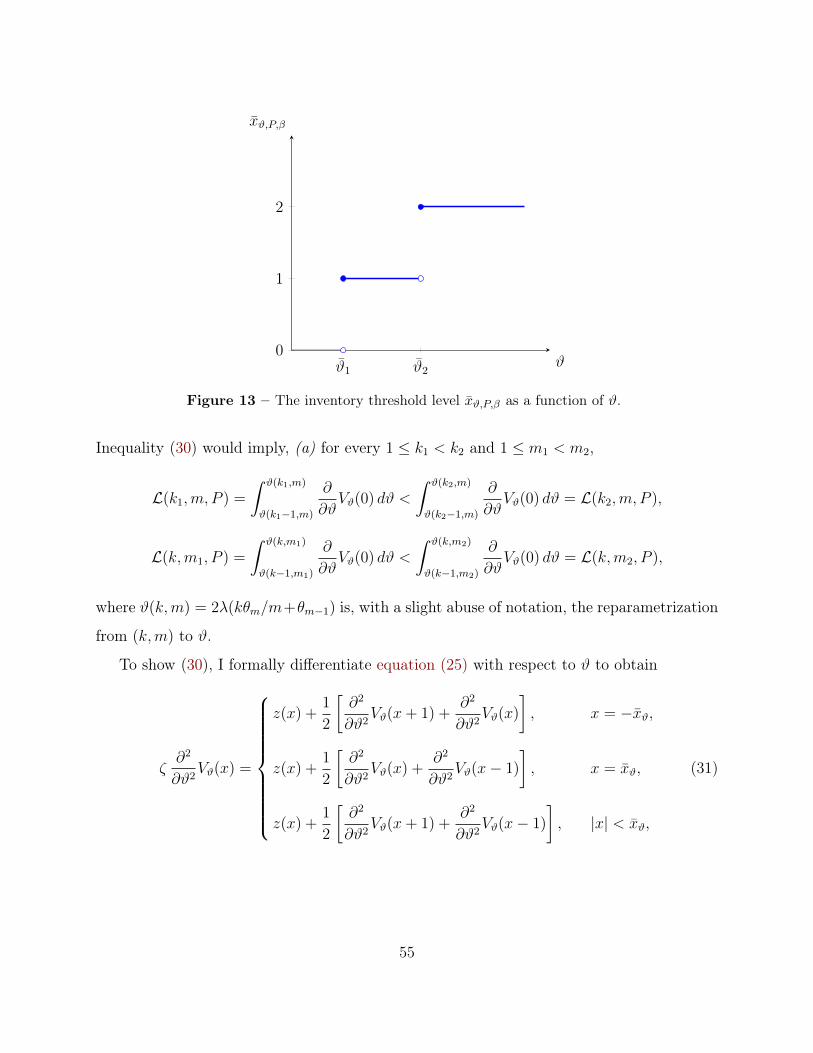
ϑ1 ϑ2

0

1

2

ϑ

xϑ,P,β

Figure 13 – The inventory threshold level xϑ,P,β as a function of ϑ.

Inequality (30) would imply, (a) for every 1 ≤ k1 < k2 and 1 ≤ m1 < m2,

L(k1,m, P ) =

∫ ϑ(k1,m)

ϑ(k1−1,m)

∂

∂ϑVϑ(0) dϑ <

∫ ϑ(k2,m)

ϑ(k2−1,m)

∂

∂ϑVϑ(0) dϑ = L(k2,m, P ),

L(k,m1, P ) =

∫ ϑ(k,m1)

ϑ(k−1,m1)

∂

∂ϑVϑ(0) dϑ <

∫ ϑ(k,m2)

ϑ(k−1,m2)

∂

∂ϑVϑ(0) dϑ = L(k,m2, P ),

where ϑ(k,m) = 2λ(kθm/m+θm−1) is, with a slight abuse of notation, the reparametrization

from (k,m) to ϑ.

To show (30), I formally differentiate equation (25) with respect to ϑ to obtain

ζ∂2

∂ϑ2Vϑ(x) =

z(x) +1

2

[∂2

∂ϑ2Vϑ(x+ 1) +

∂2

∂ϑ2Vϑ(x)

], x = −xϑ,

z(x) +1

2

[∂2

∂ϑ2Vϑ(x) +

∂2

∂ϑ2Vϑ(x− 1)

], x = xϑ,

z(x) +1

2

[∂2

∂ϑ2Vϑ(x+ 1) +

∂2

∂ϑ2Vϑ(x− 1)

], |x| < xϑ,

(31)

55

where ζ = 1/δ > 1, and

z(x) =

1

ϑ

[∂

∂ϑVϑ(x+ 1)− ∂

∂ϑVϑ(x)

], x = −xϑ,

1

ϑ

[∂

∂ϑVϑ(x− 1)− ∂

∂ϑVϑ(x)

], x = xϑ,

1

ϑ

[∂

∂ϑVϑ(x+ 1) +

∂

∂ϑVϑ(x− 1)− 2

∂

∂ϑVϑ(x)

], |x| ≤ xϑ,

Since the function ∂∂ϑVϑ is U-shaped, it follows that the function z is even and

x∑x=−x

z(x) =

2

ϑ

[∂

∂ϑVϑ(x+ 1)− ∂

∂ϑVϑ(x)

]> 0, for 0 ≤ x < xϑ,

0, for x = xϑ.

(32)

The linear system (31) can be written into the matrix form

A∂2

∂ϑ2Vϑ = z, (33)

Solving the linear system (33), one obtains ∂2

∂ϑ2Vϑ = A−1z. In particular,

∂2

∂ϑ2Vϑ(0) =

xϑ∑x=−xϑ

A−10,x · z(x) =

xϑ−1∑x=0

(A−1

0,x − A−10,x+1

) x∑x=−x

z(x) > 0.

The last inequality follows from (32) and property (iii) of Lemma 5.

Let ϑ1, ϑ2 ∈ R+ be such that xϑ1 = xϑ2 . Integrate equation (31) with respect to ϑ, for ϑ

from ϑ1 to ϑ2, and compare to the equations (25), one obtains,

∂

∂ϑVϑ2 −

∂

∂ϑVϑ1 =

∫ ϑ2

ϑ1

∂2

∂ϑ2Vϑ dϑ.

In particular,∂

∂kVk2,d,P (0)− ∂

∂kVk1,d,P (0) > 0.

56

Let ϑ0 be a discontinuity point of xϑ0 . That is, ϑ0 ∈ R+ is such that

limϑ↑ϑ0

xϑ ≡ x− < xϑ0 . (34)

The same argument used in the proof of Lemma 7 implies that for every x ∈ Z,

limϑ↑ϑ0

∂

∂ϑVϑ(x) = V (x),

where the function V is the unique solution to the fixed point problem

V (x) =

δy(x) +δ

2

[V (x+ 1) + V (x)

], x ≤ −x−,

δy(x) +δ

2

[V (x) + V (x− 1)

], x ≥ x−,

δy(x) +δ

2

[V (x+ 1) + V (x− 1)

], |x| < x−,

On the other hand, the function ∂∂ϑVϑ is the unique solution to the fixed point problem

∂

∂ϑVϑ0 = Tϑ0

(∂

∂ϑVϑ0

),

where the operator Tϑ0 is defined in (26). Starting from the function V 0 = V , let the

sequence(V `)`≥0

be generated through iterations of the operator Tϑ0 . Because x− < xϑ0

(as in (34)) and the function V 0 is U-shaped, one has

V 1(x)

= V 0(x) |x| < x−,

> V 0(x) x− ≤ |x| < xϑ0 ,

= V 0(x) |x| ≥ xϑ0 .

Thus, V 0 ≤ V 1. It then follows from the monotonicity of Tϑ0 that V h ≤ V h+1 for every

h ≥ 0. Letting h→∞, one has

limϑ↑ϑ0

∂

∂ϑVϑ = V ≤ ∂

∂ϑVϑ0 .

57

For every pair 0 ≤ ϑ1 < ϑ2,

∂

∂ϑVϑ2(0)− ∂

∂ϑVϑ1(0) ≥

∫ ϑ2

ϑ1

∂2

∂ϑ2Vϑ(0) dϑ > 0.

This establishes (30) and thus completes the proof of part (a) of Lemma 4.

I write L(k, d, P, β) for L(k, d, P ) to make clear the dependence on β.

Proposition 11. The loss L(k, d, P, β) in strictly decreasing in β ∈ R++.

The same technique used in the proof of parts (a) and (b) of Lemma 4 can be applied to

show Proposition 11. One should apply the continuity property of Vk,d,P,β in β (in Lemma 7)

and the monotonicity of xk,d,P,β in β (in Figure 13). The proof is omitted.

Proof of Lemma 4 part (c). It is easy to see that for every constant η > 0, Vk,d,ηP,ηβ =

ηVk,d,P,β. For every P2 > P1, let η = P2/P1 > 1, then

L(k, d, P2, β) > L(k, d, P2, ηβ) = ηL(k, d, P1, β) > L(k, d, P1, β).

That is, L(k, d, P, β) is strictly increasing in P ∈ R+. The continuity of L(k, d, P, β) in P is

implied by that of Vk,d,P (0) as per Lemma 7.

B.6 Proof of Theorem 1

Part (a): I fix some integer m such that 0 ≤ m ≤ m∗. Given an agent i ∈ N , suppose

all other agents follow their respective equilibrium strategies in σ∗(m). When i receives a

trade order from her outside investors, her expected gain from search is θm[π − P ∗(m)] > 0.

Otherwise, her expected gain from search is 0. Thus, agent i optimally searches among her

dealer counterparties upon receiving an outside order. Conditional on successfully reaching a

quote provider, agent i optimally trades at a given quote offer if and only if her intermediation

profit is non-negative. Since quote providers are not allowed to post stub quotes that exceed

the total gain π, it is optimal for i to trade at any given quote price.

If i has trading accounts with d dealers, for some 0 ≤ d ≤ m, the total net payoff of

i if given by Φd,P ∗(m) defined in (3). Since Φd,P ∗(m) < Φd+1,P ∗(m) for 0 ≤ d ≤ m − 2 and

58

Φm−1,P ∗(m) = Φm,P ∗(m), it is strictly optimal for i to have trading accounts with m− 1 or m

dealers. Therefore, the account maintenance strategy N∗m is optimal for i.

Given a dealer j ∈ J and let all other agents follow their respective equilibrium strategies

in σ∗(m). Suppose j is the quote provider to k non-dealers (for any k ≤ n−m) at the time

she receives a Request for Quote.

• If the equilibrium spread P ∗(m) is weakly greater than the (k,m)-tightest dealer sus-

tainable spread P (k,m), then dealer j cannot be better off by posting an offer (or bid)

price that is not P ∗(m) (−P ∗(m) respectively). Then the optimization problem faced

by dealer j can be equivalently reduced to the problem Pk,m,P ∗(m). That is, the optimal

quoting strategy of j is characterized by the inventory threshold level xk,m,P ∗(m).

• If P ∗(m) < P (k,m), then it is optimal for j to gouge by offering the bid-ask price

[−π, π].

Finally, if a non-dealer i ∈ I receives a Request for Quote at time t, he conjectures that

the associated quote seeker will follow her equilibrium strategy by discontinuing her trading

account with i immediately after time t. Then it is optimal for i to gouge by offering the

bid-ask price [−π, π]. Therefore, the strategy profile σ∗(m) is a PBE in stationary strategy.

Part (b): Given an integer m > m∗, the equilibrium spread P ∗(m) is strictly less than the

tightest dealer-sustainable spread P (m). Consequently, any given dealer is strictly better off

by gouging quote seekers. Thus, σ∗(m) is not a PBE.

B.7 Proof of Theorem 2

I fix an integer m ≥ 0, and suppose G(m) is the trading network generated by some perfect

Bayesian equilibrium σ = (S, p, ρ,Nout) in stationary strategies.

Step 1: I first show that on the equilibrium path, the offer price of any given dealer j ∈ J

is some constant a∗j , and her bid price is some constant b∗j . Formally, for every non-dealer

i ∈ I, every dealer j ∈ J and every ` = 1, 2, . . . , let τi` denote the time of the `’th Request

59

for Quote of non-dealer i, and τj` denote the time of dealer j providing the `’th quote. I use

the subscripts i`, j` and i`− to denote “at time τi`,” “at time τj`,” and “right before time τi`”

respectively. It will be shown that almost surely,

aj` = a∗j , bj` = b∗j

for every ` = 1, 2, . . . .

Since the search strategy of every given agent i ∈ N is stationary, and i searches at

most a countable number of times on the equilibrium path almost surely, it must be that i

only searches upon receiving an outsider order. Conditional on successfully reaching a quote

provider, agent i optimally trades at any given quote offer (as stub quotes are banned).

On the equilibrium path, a given non-dealer i does not have asset inventory, and has

trading accounts with all the m dealers. For every dealer j ∈ J , a ∈ R and ` = 1, 2, . . . , let

Ai`(a, j) =Oi` = Buy, ai` = a, ji` = j, xi`− = 0, Nout

i`− = J,N ini`− = ∅

denote the event that non-dealer i receives an offer price a from dealer j at time τi`. Since the

account maintenance strategy N outi of non-dealer i is stationary, the set N out

i` is deterministic

and independent of ` on the event Ai`(a, j). For every dealer j ∈ J , let

a∗j = supa ∈ [−π, π] : ∀i ∈ I,Nouti` = J almost surely on the event Ai`(a, j) (35)

be the highest ask price that j may offer without triggering account termination by any

non-dealer on the equilibrium path. Likewise, for every b ∈ R, let

Bi`(b, j) =Oi` = Sell, bi` = b, ji` = j, xi`− = 0, Nout

i`− = J,N ini`− = ∅

,

and

b∗j = supb ∈ [−π, π] : ∀i ∈ I,Nouti` = J almost surely on the event Bi`(a, j). (36)

be the lowest bid price that j may post.

60

Suppose dealer j offers some ask price aj` = a (` = 1, 2, . . . ) on the equilibrium path. If

a < a∗j , then there exists some ε > 0 such that a + ε ≤ π, and offering an ask price of a + ε

would not trigger any account termination. Dealer j is thus strictly better off if she raises

her offer price by ε, contradicting the optimality of her quoting strategy p∗j . If a∗j < a ≤ π,

then by the definition (35) of a∗j , the offer price a triggers at least one account termination

by some non-dealer on the equilibrium path. This contradicts that G(m) is the equilibrium

trading network. Therefore, the offer price of dealer j is always a∗j on the equilibrium path.

Likewise, the bid price of dealer j is always b∗j on the equilibrium path.

Consequently, the offer price a∗j and the bid price b∗j do not trigger account termination

by any non-dealer. That is, for every non-dealer i ∈ I and ` = 1, 2, . . . ,

Nouti` = J almost surely on the event Ai`

(a∗j , j

)∪Bi`

(b∗j , j

).

Step 2: I next show that for every dealer j ∈ J , the bid-ask spread a∗j − b∗j is equal to P ∗(m).

The equilibrium continuation utility of any non-dealer i ∈ I at any given time t ≥ 0 is

Φ =∑j∈J

λθmm

(π − a∗j + π + b∗j

)− mc

r.

The first term is the total expected gain from trading, the second term is the total account

maintenance cost. If non-dealer i terminates his trading account with a given dealer j ∈ J ,

his continuation utility is

Φ−j =∑

j′∈J/j

λθm−1

m− 1

(π − a∗j′ + π + b∗j′

)− (m− 1)c

r.

It must be that i is indifferent towards maintaining all his trading accounts or terminating

one of them. That is, for every given dealer j ∈ J ,

Φ = Φ−j. (37)

The indifference condition holds because:

61

(i) There is no account termination on the equilibrium path, it is thus optimal for i to

maintain all his trading accounts. That is, Φ ≥ Φ−j.

(ii) If i has strict preference over maintaining all his trading accounts (that is, if Φ > Φ−j),

then i would never terminate his account with dealer j given any quote offer. Likewise,

all other quote seekers would never terminate their accounts with j. It is then optimal

for dealer j to post the highest offer price π and the lowest bid price −π. Non-dealer

i would then be strictly better off terminating his account with j, a contradiction.

It then follows from the indifference conditions (37) that P ∗j does not depend on j ∈ J . To

show this, let j1 = argmaxj P∗j and j2 = argmaxj P

∗j be the dealer offering the largest and

the smallest spread respectively. If P ∗j1 > P ∗j2 , then terminating the trading account with

j1 is strictly better for a non-dealer than terminating the trading account with j2. That is,

Φ−j1 > Φ−j2 , which contradicts the indifference conditions (37). Thus, P ∗j1 = P ∗j2 . Therefore,

there exists some constant P ∗ such that P ∗j = P ∗ for every j ∈ J .

The total net equilibrium payoff of a non-dealer is then Φ = Φm,P ∗ , where Φd,P is given

by (3). The total continuation utility of a non-dealer after terminating one trading account

is given by Φm−1,P ∗ . The non-dealer indifference condition Φm,P ∗ = Φm−1,P ∗ implies P ∗ =

P ∗(m), where P ∗(m) is the equilibrium spread given in (5).

B.8 Proof of Theorem 3

For any given integer m ≥ 0, suppose G(m) is the trading network generated by some perfect

Bayesian equilibrium in stationary strategies. For a given dealer j ∈ J , let a∗ = P ∗(m) + h

and b∗ = −P ∗(m)+h be her equilibrium offer and bid prices respectively, for some h ∈ R. The

optimal quoting strategy of dealer j should solve the following stochastic control problem:

Dealer’s problem:

• The state space is the set Z of integers, the inventory space of dealer j.

• The control space is b∗, b∗CB×a∗, a∗CB, which is the set of all possible bid-ask quotes

that dealer j may offer.

62

• Dealer j receives Requests for Quote from k non-dealers and m− 1 dealers at the total

mean contact rate 2λ(kθm/m+θm−1). Every contacting non-dealer seeks to buy or sell

1 unit of the asset, independently across contacts and with equal probability 1/2.

• The payoff of dealer j is the expected discounted value of all her monetary transfers

and inventory cost, as specified in (2).

Let P(k, h) denote this problem. The number k of non-dealer customers will be set to be

k = n−m. Let Vk,h be the value function of the dealer in the control problem P(k, h). Then

Vk,h satisfies the HJB equations

rVk,h(x) = −βx2 + λ

(kθmm

+ θm−1

)[Vk,h(x+ 1)− Vk,h(x) + P ∗(m)− h]+

+ λ

(kθmm

+ θm−1

)[Vk,h(x− 1)− Vk,h(x) + P ∗(m) + h]+.

(38)

I extend the domain of the value function Vk,h from Z to R. That is, the HJB equation

(38) holds for every x ∈ R. It follows again from the Blackwell’s sufficient conditions and

the Contraction Mapping Theorem that there is a unique function Vk,h : R → R such that

Vk,h is bounded above by some constant and below by the function R 3 x 7→ −βx2/r, and

Vk,h satisfies the HJB equations (38). It follows from Lemma 6 and value iteration that the

function Vk,h is strictly concave.

Let y : R→ R be defined by

yh(x) = Vk,h(x) +β

rx2

for every x ∈ R. Then it follows from the HJB equations (38) that for every x ∈ R,

yh(x) =δ

2

([yh(x+ 1)− β(2x+ 1)

r+ P − h

]∨ yh(x)

+

[yh(x− 1) +

β(2x− 1)

r+ P + h

]∨ yh(x)

),

(39)

where δ is given by equation (23) with d = m. Another application of the Contraction

63

Mapping Theorem implies that the function yh is uniquely determined by the equations

(39). It follows from value iteration that the function y0 is even and strictly convex. Thus,

it must be that y0 is a continuous function on R. It can be verified that

yh(x) = y0

(x+

rh

2β

)for every x ∈ R. That is, yh is obtained by simply shifting the function y0 to the left by

rh/(2β). The functions yh and thus Vh,k are continuous. Since Vh,k is strictly concave, there

exists a unique xk,h ∈ R and xk,h ∈ R such that

Vk,h(xk,h − 1)− Vk,h(xk,h) = P ∗(m)− h,

Vk,h(−xk,h + 1)− Vk,h(−xk,h) = P ∗(m) + h.

The threshold inventory levels xk,h and −xk,h can be obtained by shifting xk,0 and −xk,0 to

the left by rh/(2β) units:

xk,h = xk,0 −rh

2β, −xk,h = −xk,0 −

rh

2β.

In the problem P(k, h), Dealer j optimally controls her inventory size within the range

[−xk,h, xk,h]. I next consider whether Dealer j has incentive to gouge. The static incentive

by the dealer to gouge is

Π(h) = max π − a∗, π + b∗ = π − P ∗(m) + |h|.

If dealer j gouges, her continuation value is at least Vk−1,h (she can achieve at least this

continuation utility by simply following the quoting strategy characterized by the problem

P(k−1, h)). Thus, the dealer’s future equilibrium profits forgone due to losing one non-dealer

customer is at most

Lk,h(x) ≡ Vk,h(x)− Vk−1,h(x).

64

Therefore, a necessary condition for dealer j to have no incentive to gouge is given by

Π(h) ≤ L(k, h) ≡ k

k +m− 1minx∈Z

−xk,h≤x≤xk,h

Lk,h(x). (40)

I will show that, for every h ∈ R,

L(k, h) ≤ L(k, 0) + |h|. (41)

Then condition (40) would imply

Π(0) ≤ L(k, 0).

It follows from Corollary 1 that the condition above is equivalent to

P ∗(m) ≥ P (k,m), (42)

where P (k,m) is the tightest (k,m)-dealer-sustainable spread. When the number of non-

dealer customers of dealer j is k = n−m, condition (42) is equivalent to m ≤ m∗, where m∗

is maximum core size defined in (14). This would complete the proof of Theorem 3. Hence,

it remains to show inequality (41).

Let ϑ = 2λ(kθm/m+θm−1). I write Vϑ,h for Vk,h, xϑ,h for xk,h and xϑ,h for xk,h. I formally

differentiate Vϑ,h(x) with respect to h, and then with respect to ϑ in (38), to obtain

ζ∂

∂hVϑ,h(x) =

1

2

[∂

∂hVϑ,h(x+ 1) +

∂

∂hVϑ,h(x− 1)

], − xϑ,h + 1 ≤ x ≤ xϑ,h − 1,

1

2

[∂

∂hVϑ,h(x+ 1) +

∂

∂hVϑ,h(x)− 1

], x < −xϑ,h + 1,

1

2

[∂

∂hVϑ,h(x− 1) +

∂

∂hVϑ,h(x) + 1

], x > xϑ,h − 1.

(43)

65

ζ∂2

∂ϑ∂hVϑ,h(x)

=

ϕ(x) +1

2

[∂2

∂ϑ∂hVϑ,h(x+ 1) +

∂2

∂ϑ∂hVϑ,h(x− 1)

], − xϑ,h + 1 ≤ x ≤ xϑ,h − 1,

ϕ(x) +1

2

[∂2

∂ϑ∂hVϑ,h(x+ 1) +

∂2

∂ϑ∂hVϑ,h(x)

], x < −xϑ,h + 1,

ϕ(x) +1

2

[∂2

∂ϑ∂hVϑ,h(x) +

∂2

∂ϑ∂hVϑ,h(x− 1)

], x > xϑ,h − 1,

(44)

where ζ = 1/δ and ϕ(x) = (ζ − 1) ∂∂hVϑ,h(x)/ϑ. For any given x ∈ [−xϑ,h, xϑ,h], let ` =

bxϑ,h − xc+ bx+ xϑ,hc+ 1, s = b(`+ 1)/2c, and $ be the following vector of length `,

$ = (−1/2, 0, . . . , 0, 1/2)>,

where A is the matrix (16) of size `× `. The two systems (43) and (44) of linear equations

can be written into following matrix forms:

A∂

∂hV = $, A

∂2

∂ϑ∂hV =

(ζ − 1) ∂∂hV

ϑ=⇒ ∂2

∂ϑ∂hV =

ζ − 1

kA−2$. (45)

For every x, h ≥ 0, let i = bxk,h − xc+ 1. Then i ≤ s. It follows from (vii) of Lemma 5 that

∂2

∂ϑ∂hVϑ,h(x) =

ζ − 1

2ϑ

(−A−2

`+1−i,1 + A−2`+1−i,`

)=ζ − 1

2ϑ

(−A−2

`+1−i,1 + A−2i,1

)≥ 0. (46)

For every h ∈ R such that |rh/(2β)| ≤ 1/2,∣∣∣∣ ∂2

∂ϑ∂hVϑ,h(0)

∣∣∣∣ =ζ − 1

ϑ

(−A−2

`+1−s,1 + A−2s,1

)<

1

ϑ≤ m

2λθm. (47)

For every x ∈ R, one can show that Vϑ,h(x) is jointly continuous in (ϑ, h) ∈ R+ × R (a

continuity proof can be obtained by adapting that of Lemma 7). It then follows that for

every (ϑ1, h1) and (ϑ2, h2),

[Vϑ2,h2(x)− Vϑ1,h2(x))− (Vϑ2,h1(x)− Vϑ1,h1(x)] =

∫ ϑ2

ϑ1

∫ h2

h1

∂2

∂ϑ∂hVϑ,h(x) dh dϑ.

66

The equality above follows from a similar argument that implies equation (29). In particular,

Lk,h(x)− Lk,0(x) =

∫ ϑ(k,m)

ϑ(k−1,m)

∫ h

0

∂2

∂ϑ∂hVϑ,h(x) dh dϑ,

where ϑ(k,m) = 2λ(kθm/m+ θm−1). It then follows from (46) that for every x, h ∈ R+,

Lk,0

(x+

rh

2β

)− Lk,0(x) = Lk,h(x)− Lk,0(x) ≥ 0.

That is, the function Lk,0(·) is weakly increasing on R+. Since Lk,0(·) is even, it is weakly

deceasing on R−. Hence, for every h ∈ R,

k +m− 1

kL(k, h) = min

x∈Z−xk,h≤x≤xk,h

Lk,h(x) = minx∈Z

−xk,0≤x≤xk,0

Lk,0

(x+

rh

2β

)

= min

Lk,0

(rh

2β−⌊rh

2β

⌋), Lk,0

(rh

2β−⌈rh

2β

⌉)= min

Lk,0

(rh

2β−⌊rh

2β

⌋), Lk,0

(⌈rh

2β

⌉− rh

2β

)If rh/(2β)− brh/(2β)c ≤ 1/2, then rh/(2β)− brh/(2β)c ≤ drh/(2β)e − rh/(2β). Hence,

k +m− 1

kL(k, h) = Lk,0

(rh

2β−⌊rh

2β

⌋)= Lk,0(0) +

∫ ϑ(k,)

ϑ(k−1,m)

∫ h∗

0

∂2

∂ϑ∂hVϑ,h(0) dh dϑ.

where h∗ is such that rh∗/(2β) = rh/(2β)−brh/(2β)c ≤ 1/2. It then follows from (47) that

k +m− 1

kL(k, h) < Lk,0(0) + |h∗| ≤ Lk,0(0) + |h| = k +m− 1

kL(k, 0) + |h|.

Thus, L(k, h) < L(k, 0) + |h|. Likewise, the same inequality L(k, h) < L(k, 0) + |h| holds if

rh/(2β)− brh/(2β)c > 1/2. Therefore, (41) holds for every h ∈ R.

B.9 Proof of Proposition 3

Given some integers m < m′, one has Φm,P ∗(m) < Φm′,P ∗(m′). Therefore, every non-dealer

enjoys a higher payoff under σ∗(m′) than σ∗(m).

67

B.10 Proof of Theorem 4 and Corollary 4

The proof of Theorem 4 closely parallels those of Theorems 1 to 3, and is thus omitted. In

the directed network G(I, J), the sum of outdegrees and the sum of indegrees must be equal:

m∗n−∑

j∈J dj

m− 1=∑j∈J

(kj + dj).

Since kj ≥ k(m∗, dj) for every j ∈ J (Theorem 4), it follows from the next lemma that

m∗n ≥∑j∈J

(k(m∗, dj) +

m

m− 1dj

)≥ |J |[k(m∗, 0)− 1],

which implies

|J | ≤ m∗n

k(m∗, 0)− 1.

Lemma 9. For every integers m > 0 and d ≥ 0,

k(m, d) +m

m− 1d ≥ k(m, 0)− 1.

Proof. It follows from the definition of k(m, d) that

Π(P ∗(m)) > L(k(m, 0)− 1,m, 0, P ∗(m)). (48)

Let ϑ = 2λ(kθm/m + dθm−1/(m − 1)). With reparametrization, I write Vϑ,P for Vk,m,d,P ,

and Lϑ,P for Lk,m,d,P . It follows from (29) and (30) in the proof of Lemma 4 that Lϑ,P (0) is

strictly increasing in ϑ ∈ R+. It then follows that

L(k(m, 0)− 1,m, 0, P ∗(m)) > L(⌊

k(m, 0)− 1− m

m− 1d

⌋,m, d, P ∗(m)

).

Combining with (48), one has

Π(P ∗(m)) > L(⌊

k(m, 0)− 1− m

m− 1d

⌋,m, d, P ∗(m)

).

Therefore,

k(m, d) ≥⌊k(m, 0)− m

m− 1d

⌋≥ k(m, 0)− 1− m

m− 1d.

68

C Proofs from Section 4

C.1 Proof of Proposition 5

Part (i) is proved in the main text. Proofs for the remaining results are provided here.

Part (ii): I fix m ≥ 1 and P > 0, and suppress m and P from the subscripts to simplify

notations. For example, Vn denotes Vn−m,m,P . Since the function ∂∂ϑVϑ is U-shaped, one has,

for every integer x ≥ 0,

[Vn+1(x)− Vn+1(x+ 1)]− [Vn(x)− Vn(x+ 1)]

=

∫ ϑ(n−m+1,m)

ϑ(n−m,m)

[∂

∂ϑVϑ(x)− ∂

∂ϑVϑ(x+ 1)

]dϑ < 0.

That is, the sequence [Vn(x)−Vn(x+1)]n≥m is strictly decreasing. Thus, the sequence admits

some limit ∆∞(x).

It will be shown in the proof of Proposition 6 that xn → ∞ as n → ∞. Then for every

x ∈ Z+, x < xn for n sufficiently large, and it follows from (21) that

rVn(x)

= − βx2 + λ

((n−m)

θmm

+ θm−1

)[Vn(x+ 1) + Vn(x− 1)− 2Vn(x) + 2P ]

∼ nλθmm

[∆∞(x− 1)−∆∞(x) + 2P ]

(49)

Where the symbol ∼ indicates asymptotic equivalence as n→∞. Letting x = 0, one has

rVn(0) ∼ nλθmm

[−2∆∞(0) + 2P ]. (50)

For every x ≥ 0,

r[Vn(0)− xP ] ≤ rVn(x) ≤ rVn(0) =⇒ rVn(x) ∼ nλθmm

[−2∆∞(0) + 2P ]. (51)

By comparing the asymptotic equivalences in (49) and (51), one obtains

∆∞(x)−∆∞(x− 1) = 2∆∞(0),

69

for every x ∈ Z+. Thus

∆∞(x) = (2x+ 1)∆∞(0).

If ∆∞ > 0, then ∆∞(x) > P for x > [P/∆∞(0)− 1]/2, which implies xn < [P/∆∞(0)− 1]/2.

The last inequality contradicts with the fact that xn goes to infinity as n→∞. Therefore,

∆∞(0) = 0. It then follows from (50) that

rVn(0) ∼ 2nλθmmP. (52)

Since Ln(0) is strictly increasing in n ≥ m (see Lemma 4), it has a limit (possibly) as n→∞.

It then follows Cesàro’s Theorem that

Vn(0)

n−m=

∑nk=m+1 Lk(0)

n−mn→∞−−−→ lim

n→∞Ln(0).

The equivalence in (52) then implies that

limn→∞

Ln(0) =2λθmrm

P

One can then solve Π(P ) = L(n−m,m,P ) to obtain

limn→∞

P (n−m,m) =mrπ

2λθm +mr.

Finally, since L(n−m,m,P ) is strictly increasing in n, the tightest dealer sustainable spread

P (n−m,m) is strictly decreasing in n. Therefore, the limiting number m∗∞ of dealer is the

largest integer m such that

mrπ

2λθm +mr= lim

n→∞P (n−m,m) < P ∗(m).

with a strict inequality.

Part (iii) (dependence of m∗ on π): To indicate the dependence of endogenous variables

on the parameter π, I will write P ∗(m,π) for the equilibrium spread, and P (m,π) for the

sustainable dealer spread. The loss function L(k,m, P ) does not depend on π.

70

Given some π1 < π2, one has, for every m ≥ 1, P > 0, and ` = 1, 2,

π` − P (m,π`) = L(n−m,m,P (m,π`)).

Since the loss function L(n−m,m,P ) is strictly increasing in P (Lemma 4), it must be that

π1 − P (m,π1) < π2 − P (m,π2), P (m,π2) > P (m,π1).

That is, when the total gain per trade increases from π1 to π2, the increase in the dealer

sustainable spread P (m,π) is strictly less than π2 − π1. On the other hand, one has

P ∗(m,π2)− P ∗(m,π1) = π2 − π1.

That is, the equilibrium spread increases more than the dealer sustainable spread. Therefore,

the core size m∗ is weakly increasing in π.

Part (iii) (dependence of m∗ on λ): The same technique used in the proof of Lemma 4 can

be applied to show that the loss L(k,m, P ) from gouging is strictly increasing in λ, for every

k ≥ 1 and P > 0. Hence, the dealer-sustainable spread P (m) is strictly decreasing in λ. On

the other hand, the equilibrium spread P ∗(m) is strictly increasing in λ (see expression (5)).

Therefore, the core size m∗ is weakly increasing in λ.

Part (iii) (dependence of m∗ on c): As c decreases, P ∗(m) increases, while P (m) is not

affected. The core size m∗ thus weakly increases.

Part (iii) (dependence of m∗ on β): For every m ≥ 1, k ≥ 1 and P > 0, the loss function

L(k,m, P, β) is strictly decreasing in β ∈ R++ (Proposition 11). Thus, the dealer sustainable

spread P (m) is strictly increasing in β. However, the equilibrium spread P ∗(m) does not

depend on β. Therefore, the core size m∗ is weakly decreasing in β.

Part (iv): When β increases or n decreases, the equilibrium number m∗ of dealers weakly

decreases. With less competition, dealers widen their equilibrium spread offer. This can be

seen directly from expression (5) of the equilibrium spread P ∗(m∗).

71

C.2 Proof of Proposition 6

Proposition 10 shows that xn−m,m,P ∗(m) is weakly decreasing in β and weakly increasing in

nλ. To drive the desired asymptotic, I fix some m ≥ 1 and P > 0, and let ϑ = 2λ((n −

m)θm/m + θm−1). With reparametrization, I write Vϑ for Vn−m,m,P and xϑ for xn−m,m,P . It

is sufficient to show that xϑ = Θ(ϑ1/3

)as ϑ goes to infinity. It follows from (6) that

Vϑ(x) = T1(Vϑ)(x), − xϑ < x < xϑ. (53)

Vϑ(x) = T2(Vϑ)(x), x ≥ xϑ. (54)

where for every function V : Z→ R,

T1(V )(x) =1

ϑ+ r

(−βx2 +

ϑ

2[V (x− 1) + V (x+ 1) + 2P ]

)

T2(V )(x) =1

ϑ+ r

(−βx2 +

ϑ

2[V (x− 1) + V (x) + P ]

).

Each of the two equations above is a difference equation. The strategy of the proof is to

solve for solutions of the two difference equations in their respective regions, then pin down

the undetermined coefficients of the solutions by some conditions on the boundaries xϑ.

One can solve for a quadratic solution U0ϑ of the first difference equation ((53)):

U0ϑ(x) = −β

rx2 +

ϑ

r

(P − β

r

).

To solve for all solutions of equation (53), I consider its homogeneous version:

rV (x) =ϑ

2[V (x− 1) + V (x+ 1)− 2V (x)]. (55)

The set of solutions to the difference equation above forms a 2-dimensional vector space

aedϑx + aedϑx : a, a ∈ R.

where

dϑ =

√2r

ϑ+O

(ϑ−

32

). (56)

72

Therefore, the solutions of equation (53) are

Z 3 x 7→ −βrx2 +

ϑ

r

(P − β

r

)+ aedϑx + ae−dϑx,

where a, a ∈ R. The value function Vϑ must be equal to one of the solutions Uϑ in the region

−xn ≤ x ≤ xn, for some a = aϑ and a = aϑ. Since the function Vϑ is even, one must have

aϑ = aϑ. Hence, for every integer x ∈ [−xϑ, xϑ],

Vϑ(x) = Uϑ(x) ≡ −βrx2 +

ϑ

r

(P − β

r

)+ aϑ cosh(dϑx), . (57)

By solving the second difference equation ((54)), one obtains, for every integer x ≥ xϑ − 1,

Vϑ(x) = Wϑ(x) ≡ W 0n(x) + bϑe

cϑx

≡ −βrx2 +

ϑ

r

β

rx−

(ϑ

r

)2β

2r+

ϑ

2r

(P − β

r

)+ bϑe

cϑx,

(58)

for some bϑ ∈ R, where

cn = −2r

θ+ 2

(rθ

)2

+O(ϑ−3). (59)

I show that the undetermined coefficients aϑ and bϑ are non-negative. For this purpose, I

define V 0ϑ as an even function from Z to R such that for every x ∈ Z+,

V 0n (x) = max

U0n(x),W 0

n(x).

Let Bϑ be the Bellman operator defined in (21). Then one hasBϑ

(V 0ϑ

)≥ T1

(V 0ϑ

)≥ T1

(U0ϑ

)= U0

ϑ,

Bϑ

(V 0ϑ

)≥ T2

(V 0ϑ

)≥ T2

(W 0ϑ

)= W 0

ϑ ,=⇒ Bϑ

(V 0ϑ

)≥ max

U0ϑ,W

0ϑ

= V 0

ϑ .

By iterating the Bellman operator Bϑ, one obtains Vϑ ≥ V 0ϑ , which implies aϑ ≥ 0, bϑ ≥ 0.

It follows from equations (57) and (58) that the functions Uϑ and Wϑ must have same

values at x = xϑ − 1, xϑ. Therefore, one has the following boundary conditions:

Uϑ(xϑ − 1) = Wϑ(xϑ − 1), Uϑ(xϑ) = Wϑ(xϑ). (60)

73

One also has

T1(Uϑ)(xϑ) = Uϑ(xϑ) = Wϑ(xϑ) = T2(Wϑ)(xϑ) = T2(Uϑ)(xϑ),

where the last equality uses the boundary conditions (60). It then follows that

Uϑ(xϑ)− Uϑ(xϑ + 1) = P.

By an abuse of notation, I use Uϑ and Wϑ to denote the functions on the entire real line

R with the same expression given by (57) and (58) respectively. Given that Uϑ is infinitely

differentiable, there exists some xϑ ∈ (xϑ, xϑ + 1) such that

U ′ϑ(xϑ) = −P. (61)

Similarly, there exists some xϑ ∈ (xϑ − 1, xϑ + 1) such that

W ′ϑ(xϑ) = −P, (62)

The boundary conditions (60) to (62) are sufficient to pin down the asymptotics of the

undetermined coefficients aϑ, bϑ as well as xϑ, as ϑ goes to infinity. Plugging the expressions

of Uϑ and Wϑ into (60) to (62), one obtains

−2β

rxϑ + aϑdϑ sinh(dϑxϑ) = −P, (63)

−2β

rxϑ +

ϑ

r

β

r+ bϑcϑe

cϑxϑ = −P. (64)

ϑ

2r

(P − β

r

)+ aϑ cosh(dϑxϑ) =

ϑ

r

β

rxϑ −

[ϑ

r

]2β

2r+ bϑe

cϑxϑ , (65)

Equation (64) and bn ≥ 0 imply that

0 ≤ − rϑbϑcϑe

cϑxϑ =β

r

(1− 2r

ϑxϑ

)+r

ϑP.

Thus, bϑecϑxϑ = O(ϑ2) and xϑ ≤ ϑ2r

for ϑ sufficiently large. By multiplying equation (64) by

74

(n−m)ϑ/(2r) and subtracting by equation (65), one obtains

aϑ cosh(dϑxϑ) = bϑO(ϑ−1)ecϑxϑ +O(ϑ) = O(ϑ). (66)

I show that xϑ = o(ϑ). Suppose this is not the case, then there exists a sequence (ϑ`)`≥0

going to infinity and xϑ` = Θ(ϑ`) as ` goes to infinity. It then follows from (63) that

aϑ` sinh(dϑ`xϑ`) = Θ(ϑ

3/2`

), thus aϑ` cosh(dϑ`xϑ`) = Θ

(ϑ

3/2`

).

This contradicts equation (66). Therefore, x = o(ϑ), and thus xϑ = o(ϑ).

I multiply (64) by ϑ/(2r) and subtract by (65), to derive a higher order Taylor expansion

aϑ cosh(dϑxϑ) =β

r

ϑ

r+O(1). (67)

=⇒ aϑdϑ sinh(dϑxϑ) ∼ 2β

r

√ϑ

rtanh(dϑxϑ).

It then follows from equation (63) that

dϑxϑ ∼ tanh(dϑxϑ).

However, the equation y = tanh y does not have any non-zero solution. Thus, limϑ dϑxϑ = 0.

A Taylor expansion applied to equation (67) leads to

aϑ =βϑ

r2+O

(βϑ

r2d2ϑx

2ϑ

). (68)

Using equation (68), another Taylor expansion applied to equation (63) leads to

aϑ d4ϑ x

3ϑ +O

(βϑ

r2d4ϑx

3ϑ

)= −P,

which implies

xϑ = Θ(ϑ1/3

), xϑ = Θ

(ϑ1/3

).

75

C.3 Proof of Proposition 8

Part (i): For some integer m ≥ 1 and P > 0, let ϑ = 2λ((n − m)θm/m + θm−1). With

reparametrization, I write C(ϑ) for C(n, λ,m). The dealer payoff Vϑ(0) increases superlin-

early with ϑ, as shown by the proof of Lemma 4. Thus, the individual dealer inventory cost

C(ϑ) is strictly concave in ϑ. On the other hand,

Vϑ(0) ≤ ϑP

r.

Thus, C(ϑ) ≥ 0. Hence, it must be that C(ϑ) is strictly increasing in ϑ ∈ R+.

Part (ii): Equation (68) implies that aϑ = βϑ/r2 +O(ϑ2/3

). Letting x = 0 in (57), one has

Vϑ(0) =ϑP

r+O

(ϑ

23

),

which implies C(ϑ) = O(ϑ2/3

).

Part (iii): Let ϑm = 2λ((n −m)θm/m + θm−1), to make clear the dependence of the total

rate ϑ of Requests for Quote on m. Then

mϑm < (m+ 1)ϑm+1.

Since the individual dealer inventory cost C(ϑ) is strictly increasing and strictly concave in

ϑ, it follows from Jensen’s inequality that

mC(ϑm) = mC(ϑm) + C(0) < (m+ 1)C

(mϑmm+ 1

)< (m+ 1)C(ϑm+1).

C.4 Proof of Proposition 9

In the outcome induced by σ∗∗(m) (0 ≤ m ≤ m), the payoff Φm,P ∗(m) of a non-dealer is given

by.

Φm,P ∗(m) =2λθm(π − P ∗(m))−mc

r,

76

As n goes to infinity, the net payoff Vn−m,m,P ∗(m)(0) of a given dealer has the following

asymptotic equivalence (see (52)):

Vn−m,m,P ∗(m)(0) ∼ 2nλθmmP ∗(m).

Thus, the welfare U(σ∗(m)) satisfies

U(σ∗(m)) = (n−m)Φm,P ∗(m) +mVn−m,m,P ∗(m)(0)

∼(

2λθmπ −mcr

)n =

[ ∑1≤m′≤m

(θm′ − θm′−1)P ∗ (m′)

]2λn

r≡ g(m)

2λn

r.

(69)

Since P ∗(m′) > 0 for every 1 ≤ m′ ≤ m, then g(m) is strictly increasing in m for 0 ≤ m ≤ m.

The asymptotic equivalence (69) implies that there exists some integer n0 > 0, if the total

number of agent n > n0, the welfare U(σ∗(m)) is strictly increasing in m for 0 ≤ m ≤ m.

D Proof of Theorem 5

To prove Theorem 5, I will need the next result about Markov Chain mixing:

Lemma 10. Let (xn)n≥0 be a sequence of strictly positive integers that goes to infinity, and

(ξn≥0) be a sequence of strictly positive reals that goes to infinity, such that x2n/ξn goes to 0

as n goes to infinity. For every n ≥ 0, let fn, gn be some functions from −xn, . . . , xn2 to

−xn, . . . , xn such that fn(x, y)+gn(x, y) = x+y for every couple (x, y). Fix some constant

ζ > 0.

For every n, let Xnt =

(Xnjt

)j∈J be a continuous-time Markov process on Z|J | with |J |

components. Suppose (Xnt )t≥0 evolves according to the following rule:

(i) At t = 0, Xn0 ∼ νn for some probability distribution νn on −xn, . . . , xn|J |.

(ii) Every Xnjt independently jumps at Poisson arrival times with intensity ξn. If −xn <

Xnjt < xn, then conditional on a jump, Xn

jt moves up by 1 unit with probability 1/2 and

moves down by 1 unit with probability 1/2. If Xnjt = xn, then conditional on a jump,

77

Xnjt moves down by 1 unit with probability 1/2 and stays at x with probability 1/2. If

Xnjt = xn, then conditional on a jump, Xn

jt moves up by 1 unit with probability 1/2 and

stays at −xn with probability 1/2. These jumps are called “individual jumps.”

(iii) Independently of (i), every couple(Xnjt, X

nj′t

)“meet” at Poisson arrival times with inten-

sity ζ. The Poisson “meeting” times are mutually independent across different meeting

pairs (j, j′). Conditional on a “meeting,” Xnjt jumps to fn

(Xnjt, X

nj′t

)and Xn

j′t jumps to

g(Xnjt, X

nj′t

). As opposed to (ii), these jumps are called “joint jumps.”

Let µn denote the uniform distribution on the set −xn, . . . , xn|J |. Let dn(t) = ||Xnt , µn||TV

for every t ≥ 0, where ||·, ·||TV denotes the total variation distance between two probability

distributions. Then for every t > 0,

dn(t)n→∞−−−→ 0.

Proof. For every n and j ∈ J , let(Xnjt

)t≥0

be the Markov process on −xn, . . . , xn which

loops at the endpoints, and otherwise jumps in the same direction as Xnjt every time Xjt

experiences an individual jump. That is, if Xnjt = xn (or −xn), then Xn

jt jumps down (up)

by 1 unit when Xnjt individually jumps down by 1 unit; If −xnXn

jt < xn, then Xnjt jumps

whenever Xnjt jumps individually, in the same direction. At t = 0, every process Xn

j0 = Xnj0.

Then every process Xnjt is a symmetric continuous-time random walk on −xn, . . . , xn,

with jump intensity ξn. The random walk Xnjt loops at the end points ±x. The processes

Xnjt are mutually independent. Therefore, the joint inventory process Xn

t ≡(Xnjt

)j∈J

has a

stationary distribution which is the uniform distribution µn on the set −xn, . . . , xn. Thus

the mixing time of this process is on the order of x2n/ξn as n goes to infinity. Since x2

n/ξn

converges to 0, then one has for every t > 0,

∥∥∥Xnt , µn

∥∥∥TV

n→∞−−−→ 0.

It should be noted that the convergence above is uniform in the initial distribution Xn0 ∼ νn.

By Proposition 4.7 of Levin, Peres, and Wilmer (2009), there exists a random variable

78

Y nt ∼ µn for every n and t ≥ 0 such that

P(Xnt 6= Y n

t

)=∥∥∥Xn

t , µn

∥∥∥TV

.

Then for every t > 0 and ε > 0, there exists nε > 0 such that for every n > nε,

P(Xnt 6= Y n

t

)< ε.

For every n and t > 0, let Dnt be the event that no pairs of Xn

jt has met by time t. Then on

the event Dnt , Xn

t = Xnt almost surely. Let (tn)n≥0 be a sequence of times converging to 0.

Then one has

P(Dntn

)= e−ζtn → 1.

It then follows that for every t > 0 and n > nε,

∥∥Xntn , µn

∥∥TV≤ P

(Xntn 6= Y n

tn

)= 1− P

(Xntn = Y n

tn

)≤ 1− P

(Xntn = Y n

tn |Dntn

)P(Dntn

)≤ 1− P

(Xntn = Y n

tn

)P(Dntn

)≤ 1− (1− ε)P

(Dntn

)→ ε.

Therefore, as n→∞, ∥∥Xntn , µn

∥∥TV→ 0 (70)

The convergence above is uniform in the initial distribution Xn0 ∼ νn. Thus for every t > 0,

‖Xnt , µn‖TV = sup

A∈Z|J||P(Xn

t ∈ A)− µn(A)|

= supA∈Z|J|

∣∣P(Xnt ∈ A |Xn

t−tn

)− µn(A)

∣∣= sup

A∈Z|J|

∣∣∣P(Xntn ∈ A | X

n0L= Xn

t−tn

)− µn(A)

∣∣∣→ 0,

where(Xnt

)is an independent copy of (Xn

t ), with the initial distribution Xn0L= Xn

t−tn .

Proof of Theorem 5. The joint inventory process (xjt) of dealers is a Markov Chain that

79

satisfies the conditions stated in Lemma 10, with ξn = 2(n −m)λθm/m and ζ = (m − 1)ς.

Thus the dealer’s problem is modified to include inter-dealer trading as follows:

Dealer’s problem P(k,m, P ):

• The state space is Z, which is the inventory space of dealer j.

• The control space is −P,−PCB × P, PCB, which is the set of all possible bid-ask

quotes that dealer j may offer.

• Dealer j receives Requests for Quote from k non-dealers and m− 1 dealers at the total

mean contact rate 2λ(θm/m+ θm−1). Every contacting non-dealer seeks to buy or sell

1 unit of the asset, independently and with equal probability 1/2.

• The payoff of dealer j is the expected discounted value of all her payments and inventory

flow cost, as specified in (2).

• Dealer j connects with another dealer j′ at the total intensity rate of (m− 1)ς.

• If dealer j has inventory x, and dealer j′ has inventory y at the time of connection,

then dealer j sells q(x, y) units of the asset to her counterpart at the price p(x, y).

• The inventory size of dealer j′ follows the uniform distribution νx on −x, . . . , x.

Let Vk,d,P be the value function of the dealer in P(k, d, P ). The terms of trade, q(x, y) and

p(x, y) are determined by maximizing the Nash Bargaining product:

[q(x, y), p(x, y)] = argmaxq∈Z,p∈R

[Vk,d,P (x− q)− Vk,d,P (x) + p

] [Vk,d,P (y + q)− Vk,d,P (y)− p

],

(71)

such that

Vk,d,P (x− q)− Vk,d,P (x) + p ≥0,

Vk,d,P (y + q)− Vk,d,P (y)− p ≥0,

That is, dealers have equal bargaining power in inter-dealer trading.

80

I conjecture, and verify later, that the value function Vk,d,P is strictly concave on Z. With

this conjecture, the Nash product (71) is maximum when

Vk,d,P (x− q)− Vk,d,P (x) + p

=Vk,d,P (y + q)− Vk,d,P (y)− p

=Vk,d,P

(⌊x+y

2

⌋)+ Vk,d,P

(⌈x+y

2

⌉)− Vk,d,P (x)− Vk,d,P (y)

2

That is, the two dealers trade q(x, y) units of the asset to equalize their inventories, and the

monetary transfer p(x, y) is such that the total gain from trade is equally shared by the two

dealers.

Therefore, the value function Vk,d,P satisfies the Hamilton–Jacobi–Bellman equation: for

every x ∈ Z,

rVk,d,P (x) = −βx2 + kλθdd

[Vk,d,P (x+ 1)− Vk,d,P (x) + P

]+

+ kλθdd

[Vk,d,P (x− 1)− Vk,d,P (x) + P

]+

+1

2(m− 1)ς

∑y∈Z

νx(y)

[Vk,d,P

(⌊x+ y

2

⌋)+ Vk,d,P

(⌈x+ y

2

⌉)

− Vk,d,P (x)− Vk,d,P (y)

].

(72)

The last term on the right hand side of the equation above corresponds to the expected change

in the dealer’s continuation utility due to inter-dealer trading. This term differentiates the

HJB equations above from the HJB equations (21) in Section 3.

The same technique can be applied to analyze the the HJB equations (72). The details

are omitted.

81

References

Adrian, T., E. Etula, and H. S. Shin, 2010, “Risk Appetite and Exchange Rates,” 2010

Meeting Papers.

Adrian, T., M. Fleming, J. Goldberg, M. Lewis, F. Natalucci, and J. Wu, 2013, “Dealer

Balance Sheet Capacity and Market Liquidity during the 2013 Selloff in Fixed Income

Markets,” FEDS Notes.

Adrian, T., E. Moench, and H. S. Shin, 2010, “Macro Risk Premium and Intermediary

Balance Sheet Quantities,” IMF Economic Review, 58(1), 179–207.

Afonso, G., A. Kovner, and A. Schoar, 2014, “Trading partners in the interbank lending

market,” working paper.

Afonso, G., and R. Lagos, 2015, “Trade Dynamics in the Market for Federal Funds,” Econo-

metrica, 83(1), 263–313.

Allen, L., and A. Saunders, 1986, “The large-small bank dichotomy in the federal funds

market,” Journal of Banking & Finance, 10(2), 219–230.

Babus, A., 2007, “The Formation of Financial Networks,” SSRN Electronic Journal.

Babus, A., and T.-W. Hu, 2015, “Endogenous Intermediation in Over-the-Counter Markets,”

SSRN Electronic Journal.

Bagwell, K., and G. Ramey, 1992, “The Diamond Paradox: A Dynamic Resolution,” working

paper.

Bech, M. L., and E. Atalay, 2010, “The topology of the federal funds market,” Physica A:

Statistical Mechanics and its Applications, 389(22), 5223–5246.

Bernheim, B., B. Peleg, and M. D. Whinston, 1987, “Coalition-Proof Nash Equilibria I.

Concepts,” Journal of Economic Theory, 42(1), 1–12.

82

Bertsekas, D. P., 2000, Dynamic Programming and Optimal Control. Athena Scientific, 2nd

edn.

Blasques, F., F. Bräuning, and I. van Lelyveld, 2015, “A Dynamic Network Model of the

Unsecured Interbank Lending Market,” Social Science Research Network Working Paper

Series.

Boss, M., H. Elsinger, M. Summer, and S. Thurner, 2004, “Network topology of the interbank

market,” Quantitative Finance, 4(6), 677–684.

Brogaard, J., 2010, “High frequency trading and its impact on market quality,” . . . University

Kellogg School of Management Working . . . .

Brogaard, J., T. Hendershott, and R. Riordan, 2014, “High-Frequency Trading and Price

Discovery,” Review of Financial Studies, 27(8), 2267–2306.

Brunnermeier, M. K., and L. H. Pedersen, 2008, “Market Liquidity and Funding Liquidity,”

Review of Financial Studies, 22(6), 2201–2238.

Cetorelli, N., B. Hirtle, D. P. Morgan, S. Peristiani, and J. Santos, 2007, “Trends in finan-

cial market concentration and their implications for market stability,” Economic Policy

Review, (Mar), 33–51.

Chang, B., and S. Zhang, 2015, “Endogenous Market Making and Network Formation,”

SSRN Electronic Journal.

Chang, E. J., E. J. A. Lima, S. M. Guerra, and B. M. Tabak, 2008, “Measures of Interbank

Market Structure: An Application to Brazil,” .

Comerton-Forde, C., T. Hendershott, C. Jones, P. Moulton, and M. Seasholes, 2010, “Time

Variation in Liquidity: The Role of Market-Maker Inventories and Revenues,” The Journal

of Finance, 65(1), 295–331.

Craig, B., and G. von Peter, 2014, “Interbank tiering and money center banks,” Journal of

Financial Intermediation, 23(3), 322–347.

83

Di Maggio, M., A. Kermani, and Z. Song, 2015, “The Value of Trading Relationships in

Turbulent Times,” SSRN Electronic Journal.

Du, S., and H. Zhu, 2014, “Ex Post Equilibria in Double Auctions of Divisible Assets,” SSRN

Electronic Journal.

Duffie, D., 2012, “Market Making Under the Proposed Volcker Rule,” SSRN Electronic Jour-

nal.

Farboodi, M., 2014, “Intermediation and Voluntary Exposure to Counterparty Risk,” SSRN

Electronic Journal.

Farboodi, M., G. Jarosh, and R. Shimer, 2015, “Who is at the Core of Financial Networks?

The Role of Meeting Technologies,” Working Paper.

Fricke, D., and T. Lux, 2014, “Core–Periphery Structure in the Overnight Money Market:

Evidence from the e-MID Trading Platform,” Computational Economics, 45(3), 359–395.

Gârleanu, N., 2009, “Portfolio choice and pricing in illiquid markets,” Journal of Economic

Theory, 144(2), 532–564.

Gromb, D., and D. Vayanos, 2002, “Equilibrium and welfare in markets with financially

constrained arbitrageurs,” Journal of Financial Economics, 66(2-3), 361–407.

, 2010, “Limits of Arbitrage,” Annual Review of Financial Economics, 2(1), 251–275.

Grossman, S. J., and M. H. Miller, 1988, “Liquidity and Market Structure,” Journal of

Finance, 43(3), 617–37.

Guo, X., and O. Hernández-Lerma, 2009, “Continuous-Time Markov Decision Processes,”

in Continuous-Time Markov Decision Processes. Springer Berlin Heidelberg, vol. 62 of

Stochastic Modelling and Applied Probability, pp. 9–18.

He, Z., and A. Krishnamurthy, 2011, “A Model of Capital and Crises,” The Review of

Economic Studies, 79(2), 735–777.

84

Heller, D., and N. Vause, 2012, “Collateral Requirements for Mandatory Central Clearing of

Over-the-Counter Derivatives,” BIS Working Papers, pp. 1–51.

Hendershott, T., D. Li, D. Livdan, and N. Schürhoff, 2015, “Relationship Trading in OTC

Markets,” Woking Paper.

Hendershott, T., and A. J. Menkveld, 2013, “Price Pressures,” Woking Paper, June(3), 1–40.

Hendershott, T., and M. S. Seasholes, 2007, “Market Maker Inventories and Stock Prices,”

American Economic Review, 97(2), 210–214.

Hollifield, B., A. Neklyudov, and C. S. Spatt, 2014, “Bid-Ask Spreads, Trading Networks

and the Pricing of Securitizations: 144a vs. Registered Securitizations,” SSRN Electronic

Journal.

Huang, Y., and W. F. McColl, 1997, “Analytical inversion of general tridiagonal matrices,”

Journal of Physics A: Mathematical and General, 30(22), 7919–7933.

Hugonnier, J., B. Lester, and P.-O. Weill, 2015, “Heterogeneity in decentralized asset mar-

kets,” Working Papers.

in ’t Veld, D., and I. van Lelyveld, 2014, “Finding the core: Network structure in interbank

markets,” Journal of Banking & Finance, 49, 27–40.

in ’t Veld, D. L., M. van der Leij, and C. H. Hommes, 2014, “The Formation of a Core

Periphery Structure in Heterogeneous Financial Networks,” SSRN Electronic Journal.

James, J., I. W. Marsh, and L. Sarno (eds.), 2012, Handbook of Exchange Rates. John Wiley

& Sons, Inc., Hoboken, NJ, USA.

Kirilenko, A. A., A. S. Kyle, M. Samadi, and T. Tuzun, 2011, “The Flash Crash: The Impact

of High Frequency Trading on an Electronic Market,” SSRN Electronic Journal.

Kyle, A. S., A. A. Obizhaeva, and Y. Wang, 2013, “Smooth Trading with Overconfidence

and Market Power,” SSRN Electronic Journal.

85

Lagos, R., G. Rocheteau, and P.-O. Weill, 2008, “Crashes and Recoveries in Illiquid Markets,”

NBER working paper.

Levin, D. A., Y. Peres, and E. L. Wilmer, 2009, Markov Chains and Mixing Times. American

Mathematical Soc.

Li, D., and N. Schürhoff, 2014, “Dealer Networks,” SSRN Electronic Journal.

Markose, S., S. Giansante, and A. R. Shaghaghi, 2012, “‘Too interconnected to fail’ financial

network of US CDS market: Topological fragility and systemic risk,” Journal of Economic

Behavior & Organization, 83(3), 627–646.

Markose, S. M., 2012, “Systemic Risk from Global Financial Derivatives: A Network Analysis

of Contagion and Its Mitigation with Super-Spreader Tax,” IMF Working Papers, 12(282).

Meli, J. A., 2002, “Do capital constraints on market makers matter? : Evidence from the

United States treasury market,” working paper.

Mengle, D., 2010, “Concentration of OTC Derivatives among Major Dealers,” working paper,

International Swaps and Derivatives Association.

MFA, 2015, “Why Eliminating Post-Trade Name Disclosure will Improve the Swaps Market,”

.

Neklyudov, A. V., 2014, “Bid-Ask Spreads and the Over-the-Counter Interdealer Markets:

Core and Peripheral Dealers,” Working Paper.

Peltonen, T. A., M. Scheicher, and G. Vuillemey, 2014, “The network structure of the CDS

market and its determinants,” Journal of Financial Stability, 13, 118–133.

Protter, P. E., 2005, Stochastic Integration and Differential Equations, vol. 21 of Stochastic

Modelling and Applied Probability. Springer Berlin Heidelberg, Berlin, Heidelberg.

Rinne, K., and M. Suominen, 2010, “Short Term Reversals, Returns to Liquidity Provision

and the Costs of Immediacy,” SSRN Electronic Journal.

86

, 2011, “A Structural Model of Short-Term Reversals,” SSRN Electronic Journal.

Rostek, M., and M. Weretka, 2012, “Price Inference in Small Markets,” Econometrica, 80(2),

687–711.

Shen, J., B. Wei, and H. Yan, 2015, “Financial Intermediation Chains in a Search Market,”

SSRN Electronic Journal.

Siriwardane, E., 2015, “Concentrated Capital Losses and the Pricing of Corporate Credit

Risk,” SSRN Electronic Journal.

Stahl, Dale O, I., 1989, “Oligopolistic Pricing with Sequential Consumer Search,” American

Economic Review, 79(4), 700–712.

Üslu, S., 2015, “Pricing and Liquidity in Decentralized Asset Markets,” Working Paper.

Vives, X., 2011, “Strategic Supply Function Competition With Private Information,” Econo-

metrica, 79(6), 1919–1966.

Weill, P.-O., 2007, “Leaning Against the Wind,” Review of Economic Studies, 74(4), 1329–

1354.

Zhang, F., 2010, “High-Frequency Trading, Stock Volatility, and Price Discovery,” SSRN

Electronic Journal.

Zhong, Z., 2013, “The Network of Inter-Dealer Trading in an Over-the-Counter Market,”

SSRN Electronic Journal.

87