the core-periphery model of regional -...

UrbEcon: Core-Periphery 1

URBAN ECONOMICS /E

Arthur O’Sullivan

Copyright: All Rights Reserved

THE CORE-PERIPHERY MODEL OF REGIONAL

AGGLOMERATION

The Core-Periphery ModelThe Symmetric EquilibriumThe Local-Competition Effect of RelocationThe Market-Access Effect of RelocationThe Cost-of-Living Effect of RelocationStability versus Instability of the Symmetric Outcome

Trade Costs and Regional AgglomerationTrade Costs and Relocation EffectsThe Core-Periphery OutcomeCommuting Costs and the Core-Periphery PatternEvidence for the Core-Periphery Model

References and Additional Reading

8


The core-periphery model of regional agglomeration is an alternative to the

neoclassical model of regional development. At the heart of the model is the second

axiom of urban economics:

Self-reinforcing changes generate extreme outcomes.

In this case, the change is migration from one region to the other, and the extreme

outcome is that most economic activity will be concentrated in one region. The label for

the model conveys the possibility that most economic activity will be concentrated in a

core region, leaving only agricultural activity in the periphery.

THE CORE-PERIPHERY MODEL

The core-periphery focuses on the location decisions of workers and firms. It is a

2 x 2 x 2 model:

• 2 regions: North and South

• 2 inputs to the production process: Skilled labor and unskilled labor

• 2 products: A manufactured good and an agricultural product

The agricultural sector is tied to land, and is modeled as a traditional sector. The

agricultural product is produced with constant returns to scale, with unskilled labor on

small family farms. Unskilled labor is assumed to be immobile, and each region has a

fixed amount of land and unskilled labor to produce agricultural products. The price of

the agricultural product is fixed, and transport cost is zero.


The manufacturing sector is modeled as a modern production sector. The modern

good is produced with skilled labor, which is perfectly mobile between the two regions.

The modern sector satisfies the fourth axiom of urban economics:

Production is subject to economies of scale.

The number of manufacturing firms is limited by increasing returns. In other words,

manufactured goods are produced in factories, not in backyards.

The model also assumes that each manufacturing firm differentiates its product,

producing one variety of the modern product. Firms in the modern industry sell different

varieties, responding to consumer preference for variety and balanced consumption.

Each consumer purchases at least a small quantity of each variety. For example, if there

are six varieties (six manufacturing firms), each consumer buys from six firms. The

bundle of products purchased by a consumer is determined by the relative prices of the

varieties: the lower the price of a particular variety, the larger the quantity purchased.

The prices of the varieties of the modern good are determined by competition and

trade costs. The larger the number of firms in a region, the more keen the competition

among firms for consumers, and the lower the prices in that region. The price of a

variety imported from other region includes the cost of transporting the product (the trade

cost), so imported varieties have higher prices than locally produced varieties.

Therefore, consumers buy larger quantities from local producers.

The Symmetric Equilibrium

Suppose we start with symmetric regions, with an equal distribution of production

between North and South. This is sensible because competing firms have an incentive to


spread themselves out to reduce direct competition. Suppose there are six varieties

produced by six firms, with the firms divided equally between the two regions. In Figure

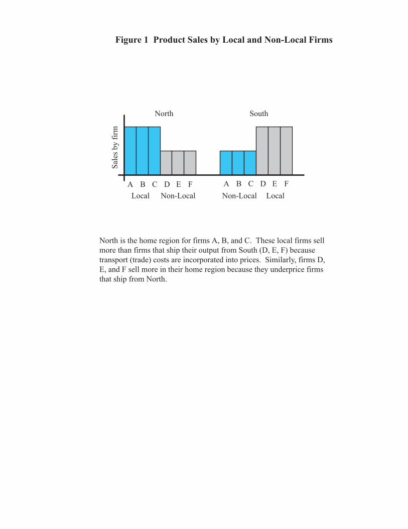
1, North has firms {A, B, C} ; South has firms {D, E, F}. In each region, each local firm

sells the same quantity to its home consumers. The non-local firms (e.g., firms D, E, F in

North) mark up their prices to cover trade (transport) costs, so they sell less than the local

firms.

The symmetric outcome is an equilibrium because there is no incentive for

workers or firms to relocate. The two regions provide the same mix of modern varieties

and the same average prices, so consumers will reach the same utility level in both

regions. With three firms in each region, workers have access to the same employment

opportunities in the two regions, so they will earn the same wages in both regions and be

indifferent between the two regions. The two regions provide the same workforce and

customer base, so firms will earn the same profit in the two regions.

The core-periphery model explores whether the symmetric outcome is stable or

unstable. To test for stability, we ask the following question: If a single firm were to

relocate from South to North, what happens next? There are two possibilities.

1. Self-Correcting Location Swap. Suppose that relocation of a firm to the North

decreases the profit of the typical original firm in the North. In this case, profit will

be higher in the South, and firms in the North will have an incentive to relocate to the

South, in effect swapping places with the firm that originally moved from South to

North. When firms swap places, the symmetric outcome is restored, indicating that it

is a stable equilibrium.

Sale

s by

fir

m

North is the home region for firms A, B, and C. These local firms sell more than firms that ship their output from South (D, E, F) because transport (trade) costs are incorporated into prices. Similarly, firms D, E, and F sell more in their home region because they underprice firms that ship from North.

Figure 1 Product Sales by Local and Non-Local Firms

A B C D E F

North South

A B C D E F

Local Non-Local LocalNon-Local


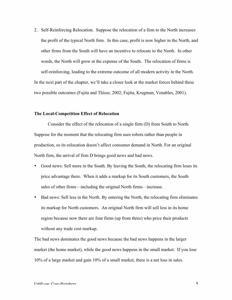
2. Self-Reinforcing Relocation. Suppose the relocation of a firm to the North increases

the profit of the typical North firm. In this case, profit is now higher in the North, and

other firms from the South will have an incentive to relocate to the North. In other

words, the North will grow at the expense of the South. The relocation of firms is

self-reinforcing, leading to the extreme outcome of all modern activity in the North.

In the next part of the chapter, we’ll take a closer look at the market forces behind these

two possible outcomes (Fujita and Thisse, 2002; Fujita, Krugman, Venables, 2001).

The Local-Competition Effect of Relocation

Consider the effect of the relocation of a single firm (D) from South to North.

Suppose for the moment that the relocating firm uses robots rather than people in

production, so its relocation doesn’t affect consumer demand in North. For an original

North firm, the arrival of firm D brings good news and bad news.

• Good news: Sell more in the South. By leaving the South, the relocating firm loses its

price advantage there. When it adds a markup for its South customers, the South

sales of other firms—including the original North firms—increase.

• Bad news: Sell less in the North. By entering the North, the relocating firm eliminates

its markup for North customers. An original North firm will sell less in its home

region because now there are four firms (up from three) who price their products

without any trade cost markup.

The bad news dominates the good news because the bad news happens in the larger

market (the home market), while the good news happens in the small market. If you lose

10% of a large market and gain 10% of a small market, there is a net loss in sales.


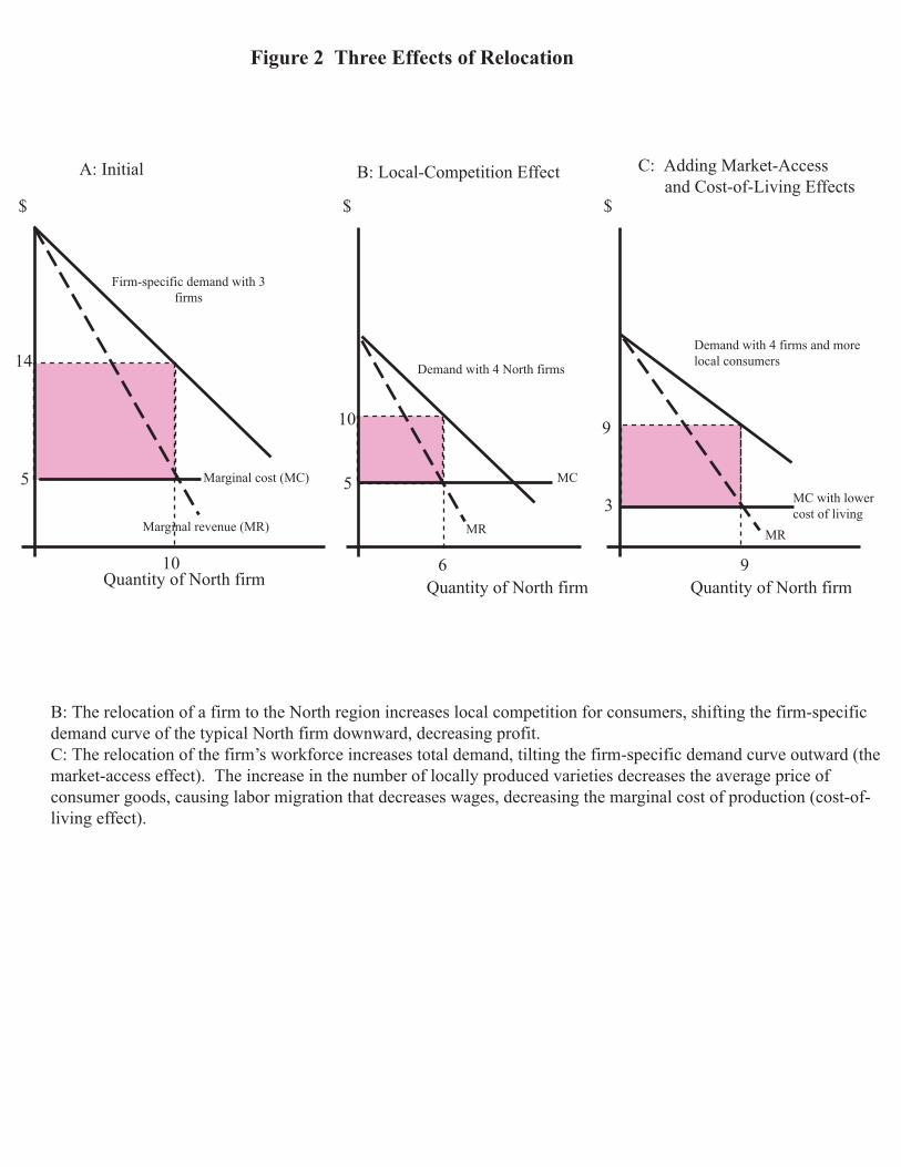
Figure 2 shows the local-competition effect of relocation from the perspective of

an original firm in the North. In Panel B, relocation shifts the firm-specific demand

curve for the typical firm downward: The increase in competition means that each firm

will sell a smaller quantity of output. A profit-maximizing firm picks the quantity at

which marginal revenue equals marginal cost. The relocation of a firm to the North

decreases the price (from $14 to $10) and decreases the quantity sold per firm (from 10 to

6).

The local-competition effect decreases the operating profit of the typical original

firm. The firm’s operating profit, shown by the shaded rectangles, equals the quantity

sold times the gap between the price and marginal cost. The relocation of firm D

decreases profit, as shown by the shrinking profit rectangle. This is similar to the normal

effect of entry into a market: more firms (more competition) means less profit per firm.

In the core-periphery model, the total number of firms in the nation doesn’t change, but

the number of firms in one region increases, so there is more competition at the local

(regional) level.

The Market-Access Effect of Relocation

The second effect of relocation is related to the movement of workers, who of

course are also consumers. Recall that the typical North firm sells some output to the

employees of firm D even when they live in the South. But when firm D relocates to the

North and its employees come along, North firms will sell their products to the new

residents without a trade-cost markup. The decrease in price will increase the quantity

$

B: The relocation of a firm to the North region increases local competition for consumers, shifting the firm-specific demand curve of the typical North firm downward, decreasing profit. C: The relocation of the firm’s workforce increases total demand, tilting the firm-specific demand curve outward (the market-access effect). The increase in the number of locally produced varieties decreases the average price of consumer goods, causing labor migration that decreases wages, decreasing the marginal cost of production (cost-of-living effect).

Figure 2 Three Effects of Relocation

$

A: Initial

Quantity of North firmQuantity of North firm

Marginal revenue (MR) MR

Demand with 4 North firms14

10 6

10

B: Local-Competition Effect

$

Quantity of North firm9

9

MC with lower cost of living

Demand with 4 firms and more local consumers

C: Adding Market-Access and Cost-of-Living Effects

Firm-specific demand with 3 firms

5 53

MR

Marginal cost (MC) MC


sold by the firm, partly offsetting the local-competition effect. Although there are more

competing firms in the region, there are also more consumers.

Panel C of Figure 2 incorporates the market-access effect of relocation. The shift

of worker-consumers to North tilts the firm-specific demand curve outward. At each

price, each firm will sell more output because it has more local consumers. This is called

the market access effect because although the total number of consumers patronizing a

firm doesn’t change, more consumers are local and thus more accessible to the typical

North firm.

The Cost-of-Living Effect of Relocation

The third effect of relocation is related to the cost of living in the growing region.

The relocation of a firm to the North increases the number of modern varieties produced

in the region, decreasing the average price of modern goods because four of the six

varieties will be sold without a trade-cost markup. Recall the first axiom of urban

economics:

Prices adjust to achieve locational equilibrium.

If consumer prices are lower in the north, perfectly mobile workers will migrate from

South to North, decreasing wages in the North. In this case, the price that adjusts to

achieve location equilibrium is the wage: Lower consumer prices result in lower wages.

Figure 2 incorporates the cost-of-living effect. In Panel C, the decrease in the

wage shifts the marginal-cost curve downward, increasing the profit-maximizing quantity

and profit. Comparing Panel C to Panel B, we see that the combined effect of the

market-access effect and the cost-of-living effect is to increase profit. Comparing Panel


C to Panel A, we see that the combined effect of all three relocation effects is to decrease

the profit of the typical original firm. In other words, the negative influence of the local-

competition effect dominates the positive influence of the market-access effect and the

cost-of-living effect.

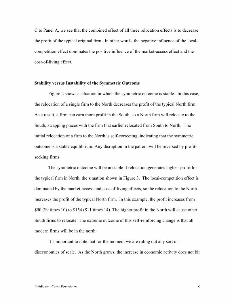
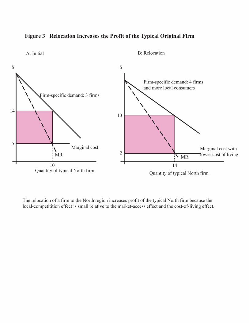
Stability versus Instability of the Symmetric Outcome

Figure 2 shows a situation in which the symmetric outcome is stable. In this case,

the relocation of a single firm to the North decreases the profit of the typical North firm.

As a result, a firm can earn more profit in the South, so a North firm will relocate to the

South, swapping places with the firm that earlier relocated from South to North. The

initial relocation of a firm to the North is self-correcting, indicating that the symmetric

outcome is a stable equilibrium: Any disruption in the pattern will be reversed by profit-

seeking firms.

The symmetric outcome will be unstable if relocation generates higher profit for

the typical firm in North, the situation shown in Figure 3. The local-competition effect is

dominated by the market-access and cost-of-living effects, so the relocation to the North

increases the profit of the typical North firm. In this example, the profit increases from

$90 ($9 times 10) to $154 ($11 times 14). The higher profit in the North will cause other

South firms to relocate. The extreme outcome of this self-reinforcing change is that all

modern firms will be in the north.

It’s important to note that for the moment we are ruling out any sort of

diseconomies of scale. As the North grows, the increase in economic activity does not bit

$

The relocation of a firm to the North region increases profit of the typical North firm because the local-competitition effect is small relative to the market-access effect and the cost-of-living effect.

Figure 3 Relocation Increases the Profit of the Typical Original Firm

A: Initial

$

Quantity of typical North firmQuantity of typical North firm

Firm-specific demand: 3 firms

MR MR

14

10

13

14

Marginal cost

B: Relocation

Marginal cost with lower cost of living

Firm-specific demand: 4 firms and more local consumers

5

2


up input prices or increase commuting time. Later in the chapter, we’ll explore the

effects of rising commuting costs.

TRADE COSTS AND REGIONAL AGGLOMERATION

We’ve seen that the symmetric outcome of equal regions may be stable or

unstable. In this part of the chapter, we’ll explore the role of trade (transport) costs in the

distribution of economic activity across regions. The issue is whether a decrease in trade

cost makes agglomeration—the core-periphery outcome—more likely. This is an

important question because of the continuing time trend of declining transport and trade

costs.

Trade Costs and Relocation Effects

We saw earlier that agglomeration occurs when the local-competition effect of

relocation is small relative to the market-access and cost-of-living effects. To explore the

effects of decreasing trade costs on the likelihood of agglomeration—the core-periphery

outcome—we must look at how each of these effects is affected by falling trade costs.

How does the local-competition effect vary with the cost of trade? Recall that this

effect occurs because relocation eliminates the trade-cost markup for the relocating firm,

increasing competition in the home market of North firms. As the unit cost of trade

decreases, the trade-cost markup diminishes, and so does the local-competition effect.

With low trade costs, there isn’t much of a markup to eliminate. In the extreme of zero

trade cost, there is no local-competition effect because competition from other firms is

the same wherever they locate.


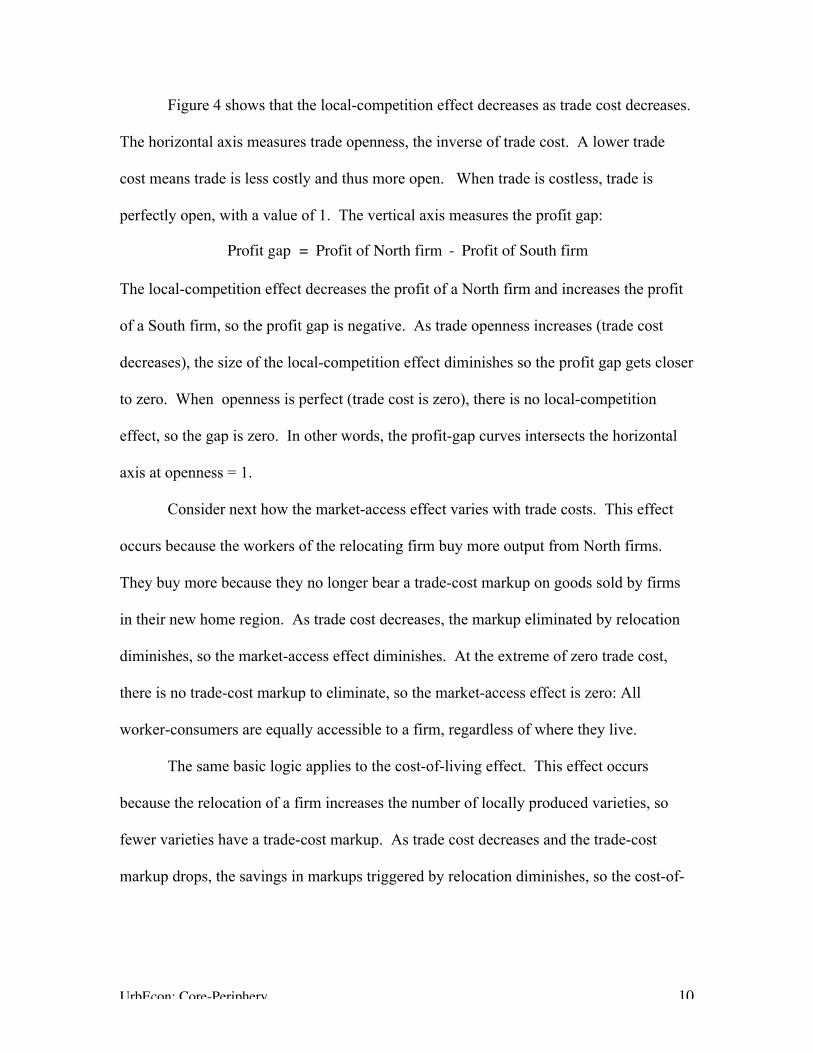
Figure 4 shows that the local-competition effect decreases as trade cost decreases.

The horizontal axis measures trade openness, the inverse of trade cost. A lower trade

cost means trade is less costly and thus more open. When trade is costless, trade is

perfectly open, with a value of 1. The vertical axis measures the profit gap:

€

Profit gap = Profit of North firm - Profit of South firm

The local-competition effect decreases the profit of a North firm and increases the profit

of a South firm, so the profit gap is negative. As trade openness increases (trade cost

decreases), the size of the local-competition effect diminishes so the profit gap gets closer

to zero. When openness is perfect (trade cost is zero), there is no local-competition

effect, so the gap is zero. In other words, the profit-gap curves intersects the horizontal

axis at openness = 1.

Consider next how the market-access effect varies with trade costs. This effect

occurs because the workers of the relocating firm buy more output from North firms.

They buy more because they no longer bear a trade-cost markup on goods sold by firms

in their new home region. As trade cost decreases, the markup eliminated by relocation

diminishes, so the market-access effect diminishes. At the extreme of zero trade cost,

there is no trade-cost markup to eliminate, so the market-access effect is zero: All

worker-consumers are equally accessible to a firm, regardless of where they live.

The same basic logic applies to the cost-of-living effect. This effect occurs

because the relocation of a firm increases the number of locally produced varieties, so

fewer varieties have a trade-cost markup. As trade cost decreases and the trade-cost

markup drops, the savings in markups triggered by relocation diminishes, so the cost-of-

Trade openness (ƒ)

Prof

it in

N -

Pro

fit i

n S

($)

0

Market access and cost-of-living effects

Local-competition effect

f*

Figure 4 Trade Openness and the Profit Gap

Combined effect

The local-competition effect decreases profit in the North and increases profit in the South. The market-access and cost-of-living effects increase profit in the North and decrease profit in the South. All three effects diminish as openness increases, reaching zero when trade is perfectly open (openness = 1). The combined effect is negative when openness is low (f < f*), but positive when openness is high (f > f*), and zero for perfect openness (f = 1).

1

-80

60

-20 • i


living effect becomes smaller. At the extreme of zero trade cost, there is no cost-of-

living effect because there are no trade-cost markups to eliminate by relocation.

The upper curve in Figure 4 shows that the market-access and cost-of-living

effects diminish as trade openness increases. Both effects increase the profit of the

typical North firm, so the profit gap is positive. When trade cost is high and openness is

low, the profit gap is relatively large. The two effects peter out as openness increases, so

the profit gap diminishes. When openness is perfect, the profit gap is zero.

The thick curve in Figure 4 shows the combined effect of all three relocation

effects. For example, at point i, the market-access and cost-of-living effects increase

profit by $60, while the local-competition effect decreases profit by $80, for a net change

of profit of -$20. When trade openness is relatively low, the local-competition effect

dominates, so the profit gap is negative. In this case, the symmetric outcome is stable:

The relocation of a firm to the North is self-correcting.

For a high degree of trade openness, the symmetric outcome will be unstable. In

Figure 4, for openness above f*, relocation to the North increases the profit of the typical

North firm because the market-access and cost-of-living effects dominate the local-

competition effect. The symmetric outcome is unstable because relocation is self-

reinforcing: After one firm relocates to the North, the higher profit there will attract other

firms. The threshold degree of openness, f* separates the stable values (f < f*) from

unstable ones (f > f*).


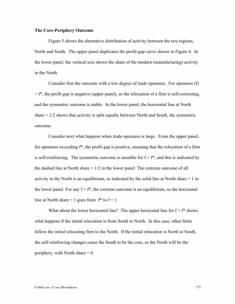
The Core-Periphery Outcome

Figure 5 shows the alternative distribution of activity between the two regions,

North and South. The upper panel duplicates the profit-gap curve shown in Figure 4. In

the lower panel, the vertical axis shows the share of the modern (manufacturing) activity

in the North.

Consider first the outcome with a low degree of trade openness. For openness (f)

< f*, the profit gap is negative (upper panel), so the relocation of a firm is self-correcting,

and the symmetric outcome is stable. In the lower panel, the horizontal line at North

share = 1/2 shows that activity is split equally between North and South, the symmetric

outcome.

Consider next what happens when trade openness is large. From the upper panel,

for openness exceeding f*, the profit gap is positive, meaning that the relocation of a firm

is self-reinforcing. The symmetric outcome is unstable for f > f*, and this is indicated by

the dashed line at North share = 1/2 in the lower panel. The extreme outcome of all

activity in the North is an equilibrium, as indicated by the solid line at North share = 1 in

the lower panel. For any f > f*, the extreme outcome is an equilibrium, so the horizontal

line at North share = 1 goes from f* to f = 1.

What about the lower horizontal line? The upper horizontal line for f > f* shows

what happens if the initial relocation is from South to North. In this case, other firms

follow the initial relocating firm to the North. If the initial relocation is North to South,

the self-reinforcing changes cause the South to be the core, so the North will be the

periphery, with North share = 0.

Trade openness (ƒ)

When trade openness is low (f < f*) , the profit gap is negative, so the symmetric outcome is stable (shown by solid line at north share = 1/2). When trade openness is high (f > f*), the profit gap is positive, so the symmetric outcome is unstable (shown by the dashed line for f >f*). If relocation occurs from North to South, activity will be concentrated in the North (shown by the solid line at North share = 1). Relocation in the opposite direction would caise concentrated in the South (shown by the solid line at North share = 0).

0

Trade openness (ƒ)

10

f*

f*

1/2

0

1

Figure 5 Trade Openness and Regional Divergence

Profit gap

1

Nor

th P

rofi

t -So

uth

Prof

itSh

are

of m

anuf

actu

ring

act

ivity

in N

orth


An important feature of this model is that the move from the symmetric outcome

to the core-periphery outcome is not gradual, but instantaneous. In the language of

economists, the switch that occurs at f* is “catastrophic.” This occurs because we have

just one modern (manufacturing) industry, and the threshold trade openness is the same

for all firms. If instead there were a variety of modern industries with different threshold

values of trade openness, the move from the symmetric outcome toward the core-

periphery outcome would be gradual rather than instantaneous.

Commuting Costs and the Core-Periphery Pattern

Up to this point, we have assumed that a region’s workforce grows, there are no

negative consequences. We know from earlier in the book that larger cities have longer

commuting distances and thus higher commuting costs and higher wages. If the

expansion of the manufacturing sector in a region occurs in cities, we expect the same

sort of negative consequences of growth.

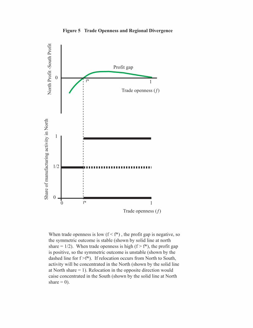
Figure 6 shows the implications of higher commuting costs and wages on the

profit-gap curve. Recall that the curve shows the profit earned by a typical North firm

minus the profit of the typical South after a single firm relocates to the North. If

relocation causes higher wages, production cost will be higher in North, so the profit gap

will be smaller. In Figure 6, the increase in the wage from longer commuting shifts the

profit-gap curve downward, generating a smaller gap at all levels of trade openness.

The downward shift of the profit-gap curve changes the core-periphery pattern.

As before, the symmetric outcome is stable for low values of trade openness. Because a

longer commute distance and a higher wage decrease the profit gap, the threshold value

Trade openness (ƒ)

Nor

th P

rofi

t -So

uth

Prof

it

Suppose the relocation of a firm to the North increases com-muting distances and costs, increasing the wage paid to manu-facturing workers. This effect shifts the profit-gap curve downward, so that the core-periphery outcome occurs for intermediate values of trade openness, between f* and f**.

0

Trade openness (ƒ)

Shar

e of

man

ufac

turi

ng a

ctiv

ity in

Nor

th

10

f*

f*

1/2

0

1

Figure 6 Commuting Cost and Regional Divergence

Profit gap with higher commuting costs

1f**

f**


of trade openness (f*) is larger: It takes a higher degree of openness to generate the core-

periphery outcome. Most important, for sufficiently high degree of trade openness, the

symmetric outcome is stable. Specifically, for openness above f**, an equal distribution

of activity between the two regions is a stable equilibrium.

The stability of the symmetric outcome for a high degree of openness may seem

puzzling. As we saw earlier, when trade costs approach zero and trade openness

approaches being perfect, all three relocation effects (local-competition, market-access,

cost-of-living) are close to zero, so the profit gap approaches zero. If relocation increases

the commuting distance and the wage, however, the negative effect of higher wages in a

larger region dominates the other (small) effects, leading to lower profit. As a result, the

relocation of one firm to the North would trigger the relocation of another firm in the

other direction. Relocation will be self-correcting rather than self-reinforcing, so the

symmetric outcome will be stable.

Evidence for the Core-Periphery Model

The core-periphery model is relatively young, and economists have only recently

started testing its validity. Head and Mayer (2004) summarize the various tests of the

theory, and conclude that so far the results are mixed, with some studies providing

evidence for the model, and others providing evidence against it. The observed

agglomerations of economic activity can be explained by other theories, and so far there

is not much evidence to support the explanations provided by the core-periphery model.

The core-periphery model predicts “catastrophic” changes in a regional economy.

The model predicts that once the threshold degree of openness is crossed, all modern


(manufacturing) activity will shift to one region or city. This suggests that cities will

either grow or shrink rapidly, implying that city sizes are unstable. In fact, city sizes are

relatively stable over time, suggesting that catastrophic changes are rare.

The core-periphery model also suggests that any region could be the core,

depending on chance or historical accident. Starting from a symmetric outcome, the

region that gets the initial shock (migration) will become the core region. One way to test

this feature of the model is to examine the effects of the bombardment of Japanese cities

in World War II. The core-periphery model suggests that a city subject to heavy damage

is likely to lose its edge, causing economic activity to shift to less damaged cities. In fact,

most bombed cities recovered rapidly, with no apparent fundamental changes in the

urban economies.

REFERENCES AND ADDITIONAL READING

1. Puga, Diego. “The Rise and Fall of Regional Inequalities.” European Economic

Review 43 (1999), pp. 303-334.

2. Fujita, Masahisa. and Jacques-Francois Thisse. Economics of Agglomeration.

Cambridge: Cambridge University Press, 2002.

3. Vernon Henderson and Jacques-Francois Thisse, eds., Handbook of Regional and

Urban Economics 4: Cities and Geography. Amsterdam: Elsevier, 2004.

• Chapter 58: Ottaviano, Gianmarco and Jacques-Francois Thisse.

“Agglomeration and Economic Geography.”

• Chapter 59: Head, Keith and Thierry Mayer. “The Empirics of

Agglomeration and Trade.”


• Chapter 62: Magrini, Stefano. “Regional (Di)Convergence.”

• Chapter 66: Kim, Sukkoo and Robert Margo. “Historical Perspectives on

U.S. Economic Geography.”

4. Baldwin, Richard, Rikard Forslid, Philippe Martin, Gianmarco Ottaviano,

Frederic Robert-Nicoud. Economic Geography and Public Policy. Princeton:

Princeton University Press, 2003.

5. Fujita, Masahisa, Paul Krugman, Anthony Venables. The Spatial Economy:

Cities, Regions, and International Trade. Cambridge: The MIT Press, 2001.

the core-periphery model of regional -...

Documents