from periphery to core: measuring agglomeration effects using high...
TRANSCRIPT

SERC DISCUSSION PAPER 172
From Periphery to Core: Measuring Agglomeration Effects Using High-Speed Rail
Gabriel M. Ahlfeldt (SERC & London School of Economics) Arne Feddersen (University of Southern Denmark)
March 2015

This work is part of the research programme of the independent UK Spatial Economics Research Centre funded by a grant from the Economic and Social Research Council (ESRC), Department for Business, Innovation & Skills (BIS) and the Welsh Government. The support of the funders is acknowledged. The views expressed are those of the authors and do not represent the views of the funders.
© G.M. Ahlfeldt and A. Feddersen, submitted 2015
From Periphery to Core: Measuring Agglomeration Effects Using High-Speed Rail
Gabriel M. Ahlfeldt* and Arne Feddersen**
March 2015
* Spatial Economics Research Centre & London School of Economics ** University of Southern Denmark We thank seminar and conference participants at Berkeley, Barcelona, London, Jonkoping, Kiel, New York, San Francisco and Vancouver, and especially Gilles Duranton, Henry Overman, Ian Gordon, Stephan Heblich, David King, and Jeffrey Lin for valuable comments and suggestions. Patricia Schikora provided excellent research assistance.

Abstract We analyze the economic impact of the German high-speed rail (HSR) connecting Cologne and Frankfurt, which provides plausibly exogenous variation in access to surrounding economic mass. We find a causal effect of about 8.5% on average of the HSR on the GDP of three counties with intermediate stops. We make further use of the variation in bilateral transport costs between all counties in our study area induced by the HSR to identify the strength and spatial scope of agglomeration forces. Our most careful estimate points to an elasticity of output with respect to market potential of 12.5%. The strength of the spillover declines by 50% ever 30 minutes of travel time, diminishing to 1% after about 200 minutes. Our results further imply an elasticity of per-worker output with respect to economic density of 3.8%, although the effects seem driven by worker and firm selection. Keywords: Accessibility, agglomeration, high-speed rail, market potential, transport policy JEL Classifications: R12; R28; R38; R48

Ahlfeldt / Feddersen –From periphery to core 2
1 Introduction
“A major new high-speed rail line will generate many thousands of construction jobs over several years, as well as permanent jobs for rail employees and increased economic activity in the destinations these trains serve.” US President Barack Obama, April 16, 2009
One of the most fundamental and uncontroversial ideas in economic geography and urban economics
is that firms and households benefit from access to economic markets due to various forms of ag-
glomeration economies (Marshall, 1920). The mutually reinforcing effects of spatial density and
productivity can theoretically account for the highly uneven distribution of economic activity be-
tween and within regions. The strong belief that economic agents benefit from an ease of interaction
has always motivated large (public) expenditures into transport infrastructures, e.g., ports, airports,
highways or railways. A striking example of an expensive, but increasingly popular transport mode is
high-speed rail (HSR). The costs of implementing an HSR network in Britain, which mainly consists of
a Y-shaped connection of London to Birmingham, Leeds, and Manchester of about 500km length are
scheduled to amount to as much as £42 (about $63) billion at present (Topham, 2013). The US De-
partment of Transportation (2009) has announced its strategic plan, which proposes the construc-
tion of completely new rail lines that will feature velocities of possibly up to 400km/h (250mph). The
plan has already identified US$8 billion plus US$1 billion a year for five years in the federal budget
just to jump-start a program that would only be comparable to the interstate highway program of the
20th century. The perhaps most spectacular HSR considered to date is a 7,000km line connecting the
Russian and Chinese capitals Moscow and Beijing, currently estimated at 1.5 trillion yuan ($242 bil-
lion) (Phillips, 2015). The willingness to commit large amounts of public money to the development
of HSR bears witness to the confidence that HSR will deliver a substantial economic impact.
The wider economic impacts such infrastructures deliver, however, naturally depend on the strength
and the spatial scope of the agglomeration economies they enhance.1 Estimating such agglomeration
effects is empirically challenging. The density of economic activity and the productivity at a given
location are not only potentially mutually dependent, but also potentially simultaneously determined
by location fundamentals, such as a favorable geography or good institutions. The main challenge in
estimating the strength and the spatial scope of agglomeration effects, therefore, is to find exogenous
1 The transport appraisal literature distinguishes between user benefits, which mainly capture the value of
shorter travel times, and wider economic impacts, such as agglomeration benefits due to higher effective
density, moves to more productive jobs, and output changes in imperfectly competitive markets
(Department for Transport, 2014).
Ahlfeldt / Feddersen –From periphery to core 3
variation in access to the surrounding economic mass. While transport infrastructures, such as a new
HSR, generate such variation in access to economic mass, the allocation of transport infrastructure is
typically non-random, thus generating additional identification problems.
In this paper we provide causal estimates of the strength and the spatial scope of agglomeration ef-
fects using a novel identification strategy. We exploit the variation in bilateral transport costs be-
tween all counties located in the German federal states of North Rhine-Westphalia, Hesse, and Rhine-
land-Palatinate that was induced by the Cologne-Frankfurt HSR. With this research design we are
able to control for unobserved time-invariant variation in location fundamentals and circumvent
some of the typical challenges in estimating the effects of spatial density on economic outcomes. Giv-
en the particular institutional setting we argue that the HSR analyzed provides variation in bilateral
transport costs that is credibly exogenous, creating a natural experiment with identifying variation
that is as good as random.
The Cologne-Frankfurt HSR was inaugurated in 2002. The line is part of the Trans-European Net-
works and facilitates train velocities of up to 300km/h. The HSR reduced travel time between both
metropolises was by more than 55% in comparison to the old rail connection and by more than 35%
in comparison to the automobile. Along the HSR line, intermediate stops were created in the towns of
Limburg, Montabaur, and Siegburg. With a population of less than 25 and 15 thousand inhabitants
and – following the connection to the HSR line – a location within 40 minutes of Cologne and Frank-
furt, which are the centers of the two largest German agglomerations, Limburg and Montabaur occu-
py a unique position on the German if not the European HSR network.
The final routing of the line and the location of the intermediate stops were the result of a political
bargaining process among the rail carrier, three federal states, and several business lobby and envi-
ronmental activist groups that lasted almost 40 years. We argue that the institutional particularities,
which we describe in more detail in section 2, allow us to make the helpful identifying assumptions
that the routing and the timing of the connection of Limburg, Montabaur, and Siegburg and the timing
of the connection of all other stations are exogenous to the levels and trends of economic develop-
ment.
Based on the exogenous variation provided, we are able to identify the causal impact of HSR on local
economic development as well as the strength and the spatial scope of agglomeration economies
promoted by the line. In the first step, we assess the effect of the HSR on the local economies within

Ahlfeldt / Feddersen –From periphery to core 4
the counties of the intermediate stops using program evaluation techniques. In the second step, we
correlate the growth in effective density, which we express in market potential form (Harris, 1954),
to the economic growth across counties within our study area. The market potential expresses effec-
tive density as the transport cost weighted sum of the GDP of all counties in the study area. The
measure takes into account the effect of the HSR on bilateral transport costs between all counties in
our study area. Since the HSR is used exclusively for passenger service we implicitly disentangle the
effects of facilitated human interactions from the transport costs of tradable goods, i.e., the trade
channel. The spillovers we capture thus include Marshallian externalities related to knowledge diffu-
sion and labor market pooling and the effects of improved access to intermediated goods and con-
sumer markets to the extent that the ease of communication reduces transaction costs, but not
freight costs.
Our results point to a positive economic impact of HSR. On average, six years after the opening of the
line, the GDP in the counties of the intermediate stops exceeds the counterfactual trend established
via a group of synthetic counties by 8.5%.2 We find an elasticity of the GDP with respect to effective
density, i.e., market potential, of about 12.5% in our most conservative model. The elasticity of out-
put per worker with respect to effective density is, at 10%, only marginally smaller. Because our
measure of effective density is spatially smoothed the variance across counties is naturally lower
than in conventional density measures. Normalized by the log ratio of the standard deviations of ef-
fective density over density our results imply an elasticity of productivity with respect to employ-
ment density of 3.8%, which is close to previous estimates derived from cross-sectional research
designs (e.g., Ciccone, 2002; Ciccone and Hall, 1996).3 The effect, however, seems to be driven to a
significant extent by selection, i.e., a compositional change in industry and worker qualification
(Combes et al., 2012). We further estimate that the strength of economic spillovers halves every 30
minutes of travel time and is near to zero after about 200 minutes. The spillovers we detect are sig-
nificantly less localized than in previous studies that have identified spillover effects from within-city
variation (Ahlfeldt et al., 2015; Ahlfeldt and Wendland, 2013; Arzaghi and Henderson, 2008), but are
2 We create a synthetic equivalents for each treated county following Adabie and Gardeazabal (2003).
3 Reviewing 729 estimates across 34 studies Melo et al. (2009) find a mean elasticity of 5.8%.
Ahlfeldt / Feddersen –From periphery to core 5
more localized than the scope of spatial interactions inferred from empirical NEG models with a
stronger emphasis on trade costs (Hanson, 2005).4
Our research connects to a large and growing literature on the nature of agglomeration economies
reviewed in detail in Duranton and Puga (2004) and Rosenthal and Strange (2004). A standard ap-
proach in this literature has been to regress economic outcome measures, such as wages, against
some measure of agglomeration, typically employment or population density.5 A smaller literature
has exploited presumably exogenous variation in the surrounding concentration of economic activi-
ty. Rosenthal and Strange (2008) and Combes et al. (2010) use geology to instrument for density.
Greenstone et al. (2010) analyze the effects of the openings of large manufacturing plants on incum-
bent plants. Another related strand has analyzed the impact of natural experiments such as trade
liberalization (Hanson, 1996, 1997), wartime bombing (Davis and Weinstein, 2002), the decrease in
the economic relevance of portage sites (Bleakley and Lin, 2014), and the Tennessee Valley Authority
(Kline and Moretti, 2014) on the spatial distribution of economic activity.
At the intersection of both strands, Redding and Sturm (2008) have exploited the effects of the varia-
tion in access to the surrounding economic mass created by the division and unification of Germany
on city growth. Ahlfeldt, et al. (2015) use the within-city variation in surrounding economic mass
induced by the division and reunification of Berlin, Germany, to identify the strength and spatial
scope of spillovers among residents and among firms as well as the rate at which commuting proba-
bilities decline in time distance. Our main contributions to this literature are twofold. First, we esti-
mate the agglomeration effects based on the variation in surrounding economic mass created by new
transport infrastructures, which allows for a relatively robust separation of spillover effects from
unobserved locational fundamental effects. Second, we contribute to a relatively small literature that
has provided estimates of the rate of spatial decay in spillovers. The relatively strong spatial decay in
spatial spillovers substantiates the intuition that moving people is more costly than moving goods.
Another growing strand in the literature to which we contribute is concerned with the economic ef-
fects of transport infrastructure. Overall, the evidence suggests that a well-developed transport in-
frastructure enhances trade (Donaldson, 2015; Duranton et al., 2013), promotes economic growth
4 See Head and Mayer (2004) for a review of this literature.
5 Examples include Ciccone (2002), Ciccone and Hall (1996), Dekle & Eaton (1999), Glaeser and Mare (2001),
Henderson, Kuncoro and Turner (1995), Moretti (2004), Rauch (1993), and Sveikauskas (1975).
Ahlfeldt / Feddersen –From periphery to core 6
(Banerjee et al., 2012; Duranton and Turner, 2012), and, at a more local level, increases property
prices (Baum-Snow and Kahn, 2000; Gibbons and Machin, 2005). There is also evidence of asymmet-
ric impacts on labor markets, in particular, of a relative increase in demand for skilled workers in
skill-abundant regions (Michaels, 2008). The evidence on the impact on the spatial distribution of
economic activity is more mixed. Within metropolitan areas radial connections tend to facilitate sub-
urbanization and, thus, benefit peripheral areas (Baum-Snow, 2007; Baum-Snow et al., 2012).6 How-
ever, there is also evidence that within larger regions reductions in trade costs between regions due
to better road networks favor core regions at the expense of peripheral regions (Faber, 2014).
Empirically, the literature evaluating the economic effects of transport infrastructure has been con-
cerned with the non-random allocation of transport infrastructure, which is usually built to accom-
modate existing or expected demand. Instrumental variables based on historic transport networks
(Duranton and Turner, 2012), counterfactual least-cost networks (Faber, 2014) or straight-line con-
nections among regional centers (Banerjee et al., 2012) have emerged as a standard approach to es-
tablishing a causal relationship. A complementary approach is to exploit the fact that the main pur-
pose of a transport infrastructure is often to connect regional agglomerations and that the connec-
tion of localities along the way is not necessarily intended (Michaels, 2008). Our contribution to this
line of research is, again, twofold. First, we provide novel evidence of the economic impacts of HSR,
an increasingly important but empirically understudied transport mode, exploiting a source of exog-
enous variation. Second, we show that peripheral regions can benefit from a better connectivity to
core regions if the cost of human interaction is reduced but trade costs remain unchanged. This evi-
dence of positive effects emerging from Marshallian externalities is complementary to the recent
evidence of negative effects on peripheral regions operating through a trade channel (Faber, 2014).
The next section introduces the institutional setting in more detail and discusses the data used. In
Section 3 we conduct a program evaluation with a focus on the impact of HSR on the economies of
the counties of the intermediate stations. In Section 4 we then exploit the full variation the HSR in-
duced in bilateral transport costs between all counties in our study area to estimate the strength and
spatial scope of agglomeration effects. The final section concludes.
6 Such a tendency of decentralization in response to reductions in transport costs is in line with standard ur-
ban models in the spirit of Alonso (1964), Mills (1967), and Muth (1969).

Ahlfeldt / Feddersen –From periphery to core 7
2 Background and data
2.1 The Cologne–Frankfurt HSR Line
The HSR line from Cologne to Frankfurt/Main is part of the priority axis Paris-Brussels-Cologne-
Amsterdam-London (PBKAL), which is one of 14 projects of the Trans-European Transport Network
(TEN-T) as endorsed by the European Commission in 1994. In comparison to the old track alongside
the river Rhine, the new HSR connects the Rhine/Ruhr area (including Cologne) and the Rhine/Main
area (including Frankfurt) almost directly, reducing track length from 222km to 177km.7 The new
track is designed exclusively for passenger transport and allows train velocities of up to 300km/h.
Due to both facts, travel time between the two main stations was reduced from 2h13 to 59min (Brux,
2002). Preparatory works for the construction of the HSR started in December 1995. The major con-
struction work —on the various tunnels and bridges— began in 1998. The HSR line was completed
at the end of 2001. After a test period the HSR line was put into operation in 2002. The total cost of
the project was 6 billion Euros (European Commission, 2005, p. 17).
The broader areas of Rhine-Ruhr and Rhine-Main have long been considered to be the largest Ger-
man economic agglomerations. The rail lines connecting the two centers along both Rhine riverbanks
were among the European rail corridors with the heaviest usage. They had represented a traditional
bottleneck since the early 1970s, when usage already exceeded capacity. The first plans for con-
structing an HSR line between Cologne and Frankfurt, consequently, date back to as far as the early
1970s. Since then, it has taken more than 30 years until the opening. A reason for the long time peri-
od was the complex evolution process of infrastructure projects in Germany. Several variants at the
left-hand and right-hand side of the Rhine were discussed during the decades of negotiations. Taking
into account the difficult geography of the Central German Uplands, it was ultimately decided to con-
struct a right-hand side connection that would largely follow the highway A3 in an attempt to mini-
mize construction and environmental costs as well as travel time between the major centers. These
benefits came at the expense of leaving relatively large cities like Koblenz and the state capitals
Wiesbaden (Hesse) and Mainz (Rhineland Palatinate) aside.
Due to the federal system of the Federal Republic of Germany the states (Länder) have a strong influ-
ence on infrastructure projects that affect their territories (Sartori, 2008, pp. 3–8). Three federal
7 The straight-line distance between Cologne Main Station and Frankfurt Main Station is 152km.

Ahlfeldt / Feddersen –From periphery to core 8
states were concerned with the subject project: North Rhine-Westphalia, Rhineland-Palatine, and
Hesse. While Cologne lies in North Rhine-Westphalia and Frankfurt is located in Hesse, no stop was
planned within the state of Rhineland-Palatine after the plans to connect Koblenz were abandoned in
1989. The announcement of the exact routing, however, suddenly opened opportunities for commu-
nities along the line to lobby in favor of their connection. Limburg, supported by Hesse, was the first
city to make a case. Somewhat later in the process, the local political and economic actors in Mon-
tabaur also managed to convince the state authorities of Rhineland-Palatinate to support their case.
It was argued that from Montabaur the hinterland of the state could be connected via an existing
regional line. The case of Montabaur was facilitated by the decision to build the new Limburg station
at the south-eastern fringe of the city in Eschhofen. The originally proposed site (Limburg Staffel)
was significantly closer than Montabaur and, given the already short distance, would have made an
additional stop in Montabaur almost impossible to justify. During a long lobbying process menacing a
blockade of the planning and political decision process, the three federal states eventually negotiated
three intermediate stops along the HSR line, one in each of the concerned federal states. While
Bonn/Siegburg and Limburg represented the shares of North Rhine-Westphalia and Hesse, a new
station in Montabaur ensured the connection of Rhineland-Palatinate.
At the end of this process, Montabaur, with a population of less than 20,000 – the by far smallest city
on the German high-speed rail network – found itself within 40 minutes of the regional centers Co-
logne and Frankfurt and within 20 minutes of the international airports Frankfurt and Cologne-Bonn.
Anecdotal evidence suggests that this exceptional upgrade in terms of accessibility improved the
attractiveness of the city as a business location. A new congress center was opened and more than 50
firms settled in an industrial park built adjacent to the rail station;8 1&1, a leading provider of com-
munication services, even moved their headquarters to that location. A number of local manufactur-
ing companies in the wider catchment area expanded their capacities in response to the improve-
ment in connectivity (Egenolf, 2008). Among the major advantages reported were the ease of main-
taining business relations and an improved access to a highly qualified labor pool. In selected firms,
more than 80% of the managerial positions are held by in-commuters. Passenger numbers have
reached 3,000 per day, about 10 times the original forecasts (Müller, 2012).
8 Among them: Landesbetrieb Mobilität RLP Autobahnamt, Unternehmensberatung EMC², Industrie- und
Handelskammer (IHK), Ingenieurgesellschaft Ruffert und Partner, Objektverwalter S.K.E.T, Cafe Latino, Kan-
tine Genuss & Harmonie.
Ahlfeldt / Feddersen –From periphery to core 9
Notwithstanding this local impact, the intermediate stops have been very controversial in terms of
their economic viability. The cities of Montabaur and Limburg only exhibit approx. 12,500 and
34,000 habitants. Furthermore, the distance between these two small cities is barely 20km and the
high-speed ICE train needs only nine minutes between both stops, which is in contrast to the concept
of high-velocity travelling that has its comparative advantages at much larger distances. The ad-
vantage of this institutional setting for our empirical analysis is that it is reasonable to assume that
the routing of the track was exogenous in the sense that it was determined by geographical con-
straints and environmental concerns. The connection of the intermediate stations was not driven by
existing or expected demand – in fact, these stations were heavily opposed by the operating rail car-
rier Deutsche Bahn. Thus, we consider the resulting variation in accessibility provided by the rail line
as exogenous to the economic outcomes we observe. Furthermore, it is reasonable to argue that the
timing of the inauguration was exogenous to contemporary economic trends for the entire line.
When the plans for a connection of Frankfurt and Cologne were first drafted in the 1970s it was vir-
tually impossible to foresee changes in economic conditions in the late 1990s.
Ahlfeldt / Feddersen –From periphery to core 10
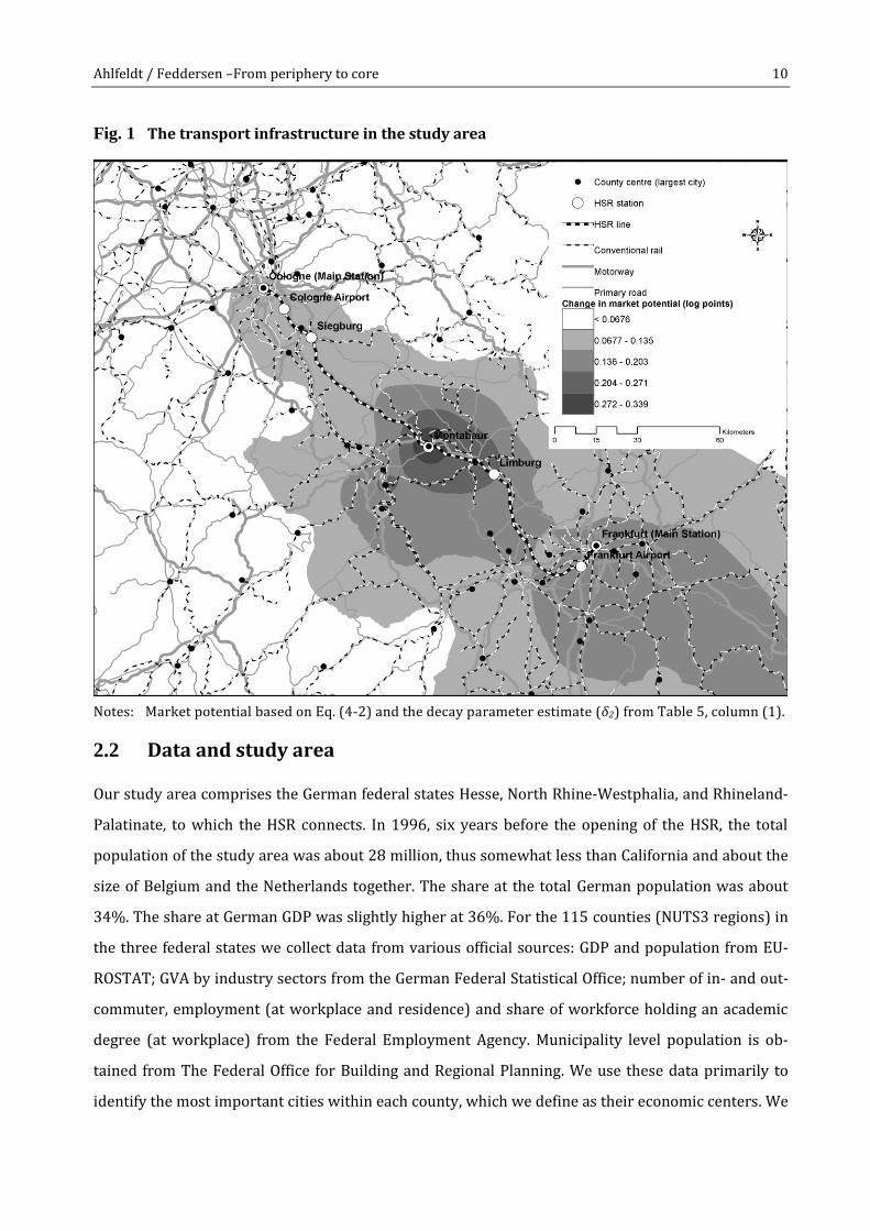
Fig. 1 The transport infrastructure in the study area
Notes: Market potential based on Eq. (4-2) and the decay parameter estimate (δ2) from Table 5, column (1).
2.2 Data and study area
Our study area comprises the German federal states Hesse, North Rhine-Westphalia, and Rhineland-
Palatinate, to which the HSR connects. In 1996, six years before the opening of the HSR, the total
population of the study area was about 28 million, thus somewhat less than California and about the
size of Belgium and the Netherlands together. The share at the total German population was about
34%. The share at German GDP was slightly higher at 36%. For the 115 counties (NUTS3 regions) in
the three federal states we collect data from various official sources: GDP and population from EU-
ROSTAT; GVA by industry sectors from the German Federal Statistical Office; number of in- and out-
commuter, employment (at workplace and residence) and share of workforce holding an academic
degree (at workplace) from the Federal Employment Agency. Municipality level population is ob-
tained from The Federal Office for Building and Regional Planning. We use these data primarily to
identify the most important cities within each county, which we define as their economic centers. We

Ahlfeldt / Feddersen –From periphery to core 11
collected data from 1992–1995 (depending on data availability) to 2009. The average county in our
study area in 1996 had a population of about 241k, which is significantly larger than the average
county in the rest of the country (157k). In terms of output per worker, our study area is fairly simi-
lar to the rest of the country (€71.5k vs. €70.8). Also, the shares of various industries at the regional
GVA are remarkably similar. Descriptive statistics are presented in section 2 of the appendix, where
we also present a map that illustrates the location of the study area and the HSR within Germany.
3 Program evaluation
The intermediate stops Limburg, Montabaur, and Siegburg on the Cologne-Frankfurt HSR were, as
we argue, an accidental result of political bargaining and not rational transport planning. The new
stations thus provide plausibly exogenous variation in transport services that can be exploited to
detect economic impact using established program evaluation techniques. In this section we analyze
the economic effects of the opening of the HSR – the treatment – on the economies of the counties of
the intermediate stops, the treated counties. Specifically, we compare the evolution of various eco-
nomic outcome measures in the treated counties to control counties that provide a counterfactual.
A – Treated vs. synthetic counties
We note that at this stage we ignore Cologne and Frankfurt because these regional centers are argu-
ably major generators of transport demand, so the routing of the high-speed rail line cannot be con-
sidered exogenous to their economic performance. As these cities potentially benefit from improved
transport services we also exclude them from the group of control counties. Besides, on the exogenei-
ty of the treatment the credibility of a quasi-experimental comparison rests on the assumption that
the treatment and control group would have followed the same trend in the absence of the treat-
ment. To ensure a valid comparison we create a comparison group consisting of three synthetic
counties, one for each of the treated counties in which the HSR stops Limburg, Montabaur, and Sieg-
burg are located. We follow the procedure developed by Abadie and Gardeazabal (2003), who define
a synthetic region as a weighted combination of non-treated regions. The optimal combination of
weights is determined by two objectives.
First, a synthetic county should match its treated counterpart as closely as possible in terms of the
following economic growth predictors: GDP per worker, population density, ratio of out-commuters
over in-commuters, the shares of construction, mining, services, retail, manufacturing, and finance at
Ahlfeldt / Feddersen –From periphery to core 12
gross value added, and the share of workers holding a university degree in the workforce at work-
place. Formally, this problem is defined as min𝑊∈𝑊(𝑋1 − 𝑋0𝑊)´𝑉(𝑋1 − 𝑋0𝑊), where W is a vector of
non-negative weights of the non-treated counties in the synthetic county that must sum to one, X1 is a
vector of pre-opening values of k economic growth predictors for the treated county, X0 is a matrix
containing the same information for the non-treated counties, and V is a diagonal matrix with non-
negative elements that determine the relative importance of the growth predictors.
The solution to this problem, the vector of optimal weights of non-treated counties W*, depends on V,
which leads to the second objective. We search for the optimal combination V* which produces a
synthetic control county that best matches the respective treated county in terms of the pre-
construction growth trend. Formally, this second problem is defined as 𝑉∗ = argmin𝑉∈𝜈(𝑍1 −
𝑍0𝑊∗(𝑉))´(𝑍1 − 𝑍0𝑊
∗(𝑉)), where Z1 a is vector of pre-construction observations of an economic
outcome measure Y for the treated county and Z0 is a matrix with the same information for the non-
treated counties.9
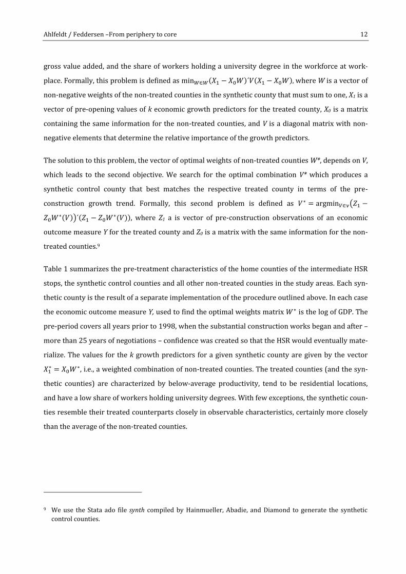
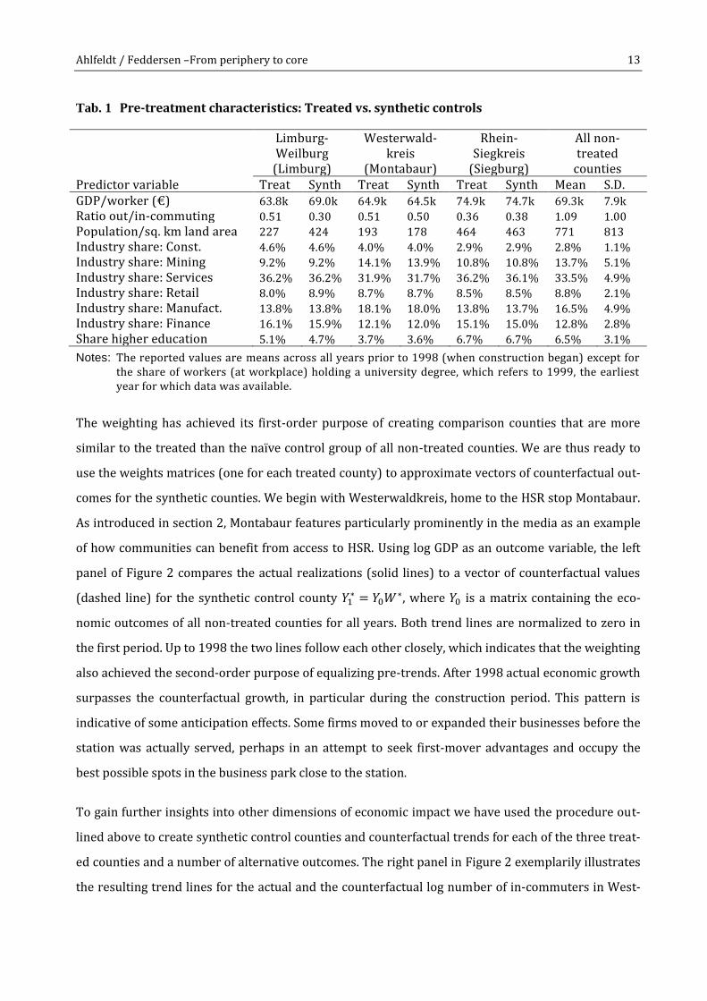
Table 1 summarizes the pre-treatment characteristics of the home counties of the intermediate HSR
stops, the synthetic control counties and all other non-treated counties in the study areas. Each syn-
thetic county is the result of a separate implementation of the procedure outlined above. In each case
the economic outcome measure Y, used to find the optimal weights matrix 𝑊∗ is the log of GDP. The
pre-period covers all years prior to 1998, when the substantial construction works began and after –
more than 25 years of negotiations – confidence was created so that the HSR would eventually mate-
rialize. The values for the k growth predictors for a given synthetic county are given by the vector
𝑋1∗ = 𝑋0𝑊
∗, i.e., a weighted combination of non-treated counties. The treated counties (and the syn-
thetic counties) are characterized by below-average productivity, tend to be residential locations,
and have a low share of workers holding university degrees. With few exceptions, the synthetic coun-
ties resemble their treated counterparts closely in observable characteristics, certainly more closely
than the average of the non-treated counties.
9 We use the Stata ado file synth compiled by Hainmueller, Abadie, and Diamond to generate the synthetic
control counties.
Ahlfeldt / Feddersen –From periphery to core 13
Tab. 1 Pre-treatment characteristics: Treated vs. synthetic controls
Limburg-Weilburg
(Limburg)
Westerwald-kreis
(Montabaur)
Rhein-Siegkreis
(Siegburg)
All non-treated
counties Predictor variable Treat Synth Treat Synth Treat Synth Mean S.D. GDP/worker (€) 63.8k 69.0k 64.9k 64.5k 74.9k 74.7k 69.3k 7.9k
Ratio out/in-commuting 0.51 0.30 0.51 0.50 0.36 0.38 1.09 1.00
Population/sq. km land area 227 424 193 178 464 463 771 813
Industry share: Const. 4.6% 4.6% 4.0% 4.0% 2.9% 2.9% 2.8% 1.1%
Industry share: Mining 9.2% 9.2% 14.1% 13.9% 10.8% 10.8% 13.7% 5.1%
Industry share: Services 36.2% 36.2% 31.9% 31.7% 36.2% 36.1% 33.5% 4.9%
Industry share: Retail 8.0% 8.9% 8.7% 8.7% 8.5% 8.5% 8.8% 2.1%
Industry share: Manufact. 13.8% 13.8% 18.1% 18.0% 13.8% 13.7% 16.5% 4.9%
Industry share: Finance 16.1% 15.9% 12.1% 12.0% 15.1% 15.0% 12.8% 2.8%
Share higher education 5.1% 4.7% 3.7% 3.6% 6.7% 6.7% 6.5% 3.1%
Notes: The reported values are means across all years prior to 1998 (when construction began) except for the share of workers (at workplace) holding a university degree, which refers to 1999, the earliest year for which data was available.
The weighting has achieved its first-order purpose of creating comparison counties that are more
similar to the treated than the naïve control group of all non-treated counties. We are thus ready to
use the weights matrices (one for each treated county) to approximate vectors of counterfactual out-
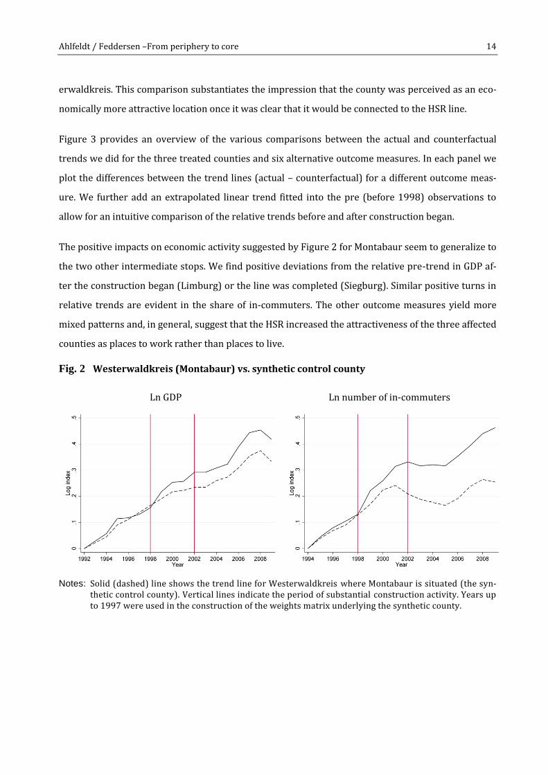
comes for the synthetic counties. We begin with Westerwaldkreis, home to the HSR stop Montabaur.
As introduced in section 2, Montabaur features particularly prominently in the media as an example
of how communities can benefit from access to HSR. Using log GDP as an outcome variable, the left
panel of Figure 2 compares the actual realizations (solid lines) to a vector of counterfactual values
(dashed line) for the synthetic control county 𝑌1∗ = 𝑌0𝑊
∗, where 𝑌0 is a matrix containing the eco-
nomic outcomes of all non-treated counties for all years. Both trend lines are normalized to zero in
the first period. Up to 1998 the two lines follow each other closely, which indicates that the weighting
also achieved the second-order purpose of equalizing pre-trends. After 1998 actual economic growth
surpasses the counterfactual growth, in particular during the construction period. This pattern is
indicative of some anticipation effects. Some firms moved to or expanded their businesses before the
station was actually served, perhaps in an attempt to seek first-mover advantages and occupy the
best possible spots in the business park close to the station.
To gain further insights into other dimensions of economic impact we have used the procedure out-
lined above to create synthetic control counties and counterfactual trends for each of the three treat-
ed counties and a number of alternative outcomes. The right panel in Figure 2 exemplarily illustrates
the resulting trend lines for the actual and the counterfactual log number of in-commuters in West-
Ahlfeldt / Feddersen –From periphery to core 14
erwaldkreis. This comparison substantiates the impression that the county was perceived as an eco-
nomically more attractive location once it was clear that it would be connected to the HSR line.
Figure 3 provides an overview of the various comparisons between the actual and counterfactual
trends we did for the three treated counties and six alternative outcome measures. In each panel we
plot the differences between the trend lines (actual – counterfactual) for a different outcome meas-
ure. We further add an extrapolated linear trend fitted into the pre (before 1998) observations to
allow for an intuitive comparison of the relative trends before and after construction began.
The positive impacts on economic activity suggested by Figure 2 for Montabaur seem to generalize to
the two other intermediate stops. We find positive deviations from the relative pre-trend in GDP af-
ter the construction began (Limburg) or the line was completed (Siegburg). Similar positive turns in
relative trends are evident in the share of in-commuters. The other outcome measures yield more
mixed patterns and, in general, suggest that the HSR increased the attractiveness of the three affected
counties as places to work rather than places to live.
Fig. 2 Westerwaldkreis (Montabaur) vs. synthetic control county
Ln GDP
Ln number of in-commuters
Notes: Solid (dashed) line shows the trend line for Westerwaldkreis where Montabaur is situated (the syn-
thetic control county). Vertical lines indicate the period of substantial construction activity. Years up to 1997 were used in the construction of the weights matrix underlying the synthetic county.

Ahlfeldt / Feddersen –From periphery to core 15
Fig. 3 Relative trends for treated counties vs. synthetic control counties
Notes: Solid lines represent the differences between the trend lines for a treated county and the synthetic
control county. Vertical lines indicate the period of substantial construction activity. Years up to 1997 were used in the construction of the weights matrices underlying the synthetic counties. Dashed lines are extrapolated linear fits using observations before 1998.

Ahlfeldt / Feddersen –From periphery to core 16
B – Econometric analysis
For a more formal test of the economic impact of the HSR on the group of treated counties we make
use of the following difference-in-differences (DD) specification:
log(𝑌𝑖𝑡) = 𝜃[𝑇𝑖 × (𝑡 > 2002)𝑡] + ∑ 𝜃𝑛[𝑇𝑖 × (𝑡 = 𝑛)]2002
𝑛=1998+ ϑ[𝑇𝑖 × (𝑡 − 2003)𝑡]
+ ϑP[𝑇𝑖 × (𝑡 − 2003)𝑡 × (𝑡 > 2002)𝑡] + 𝜇𝑖 + 𝜑𝑡 + 휀𝑖𝑡
(3-1)
, where i and t index counties (treated and non-treated) and years, 𝑇𝑖 is a dummy variable that is one
for the treated counties of Montabaur, Limburg, and Siegburg and zero otherwise, (𝑡 > 2002) simi-
larly indexes years after 2002, (𝑡 = 𝑛) similarly indexes a year n, (𝑡 − 2003) is a yearly trend taking a
value of zero in 2003, and 𝜇𝑖 and 𝜑𝑡 are county and year fixed effects and 휀𝑖𝑡 is a random error term.
This specification allows for a short-run impact on the level of the economic outcome variable
(𝜃[𝑇𝑖 × (𝑡 > 2002)𝑡]) as well as a long-run impact on its trend (ϑP[𝑇𝑖 × (𝑡 − 2003)𝑡 × (𝑡 >
2002)𝑡]) while controlling for heterogeneity in pre-trends across the treated and the control coun-
ties (ϑ[𝑇𝑖 × (𝑡 − 2003)𝑡]). The cumulated percentage impact in a given (post) year is defined as
exp (�̂� + �̂�P × (𝑡 − 2003)) − 1. 10 The new stations have provided transport services since 2002, but
a high degree of confidence regarding the eventual completion of the line have existed since 1998
when the substantial construction works began. We therefore add a number of short-run DD terms
∑ 𝜃𝑛[𝑇𝑖 × (𝑡 = 𝑛)]2002𝑛=1998 which absorb the effects during the construction period so that our treat-
ment estimates are based on a comparison between the pre-construction (t<1998) to the post-
completion period (t>2002). Essentially, the model produces empirical estimates of the cumulated
effect (and its significance) which correspond to the differences between the solid and the dashed
lines in Figure 3 during the post period. Standard errors are clustered on counties to account for se-
rial correlation as recommended by Bertrand, Duflo, and Mullainathan (2004).
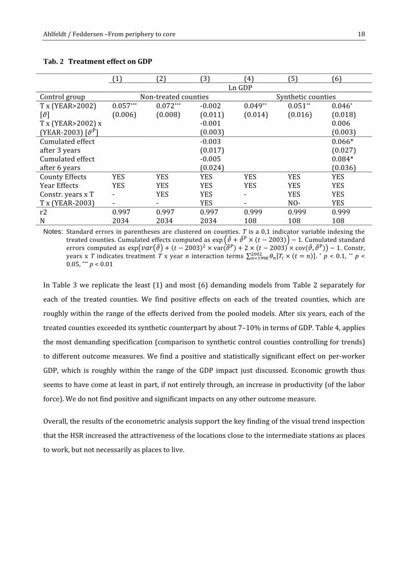
We begin with the presentation of the empirical results for the outcome measure log GDP in Table 2.
We use the groups of all non-treated (1–3) as well as the synthetic counties (4–6) as control groups
and, in each case, complement the presentation of the results of the full models (3) and (6) with sim-
plified versions of the model. Columns (1) and (4) provide a simple mean comparison (conditional on
county and year fixed effects) of the difference in log GDP across the groups of treated and non-
10 The respective standard error is exp(𝑣𝑎𝑟(�̂�) + (𝑡 − 2003)2 × var(�̂�P) + 2 × (𝑡 − 2003) × cov(�̂�, �̂�P)) − 1.

Ahlfeldt / Feddersen –From periphery to core 17
treated as well as the pre (before 2003) and post (from 2003 onwards) periods. Columns (2) and (5)
control for effects during the construction years, but do not control for trends.
The results, relatively consistently point to a positive and significant impact of the HSR on GDP. Ig-
noring trends, GDP in the treated counties grew by about 7% more in the treated counties than in the
remaining ones if the comparison is made between the periods before construction began and after
construction ended (2). The effect is slightly larger than in the basic model (1), which is consistent
with the anticipation effects found in the visual inspection of the trend lines. The effect is also rough-
ly in line with the average differences between the actual relative trend (solid lines) and linearly ex-
trapolation pre-trends (dashed lines) during the post-period in the upper-left panel of Figure 3. Once
we control for relative trends, the treatment effect disappears. As there is no positive impact on
(post) trends, the implication is that the model attributes the relative differences between the before
and after period to heterogeneous trends that existed prior to the treatment.
Our preferred models, which compare the trends in the treated counties to the synthetic counties,
yield a somewhat different picture. Consistently, all models (4–6) point to a GDP growth in the group
of treated counties that exceeds the control group by about 5% in the short run. The full model (6)
also suggests a positive long-run impact on the GDP trend, which is just about not statistically signifi-
cant. The cumulated effects after three (2006) and six (2009) years, which are a combination of the
short-run level and long-run trend effects amount to statistically significant effects of about 6.5–8.5%
and are thus within the range of the effects suggested by Table 2, column (2) and Figure 3 (upper-
left).
Ahlfeldt / Feddersen –From periphery to core 18
Tab. 2 Treatment effect on GDP
(1) (2) (3) (4) (5) (6) Ln GDP Control group Non-treated counties Synthetic counties T x (YEAR>2002) [𝜗]
0.057*** (0.006)
0.072*** (0.008)
-0.002 (0.011)
0.049** (0.014)
0.051** (0.016)
0.046* (0.018)
T x (YEAR>2002) x (YEAR-2003) [𝜗P]
-0.001 (0.003)
0.006 (0.003)
Cumulated effect -0.003 0.066* after 3 years (0.017) (0.027) Cumulated effect -0.005 0.084* after 6 years (0.024) (0.036) County Effects YES YES YES YES YES YES Year Effects YES YES YES YES YES YES Constr. years x T - YES YES - YES YES T x (YEAR-2003) - - YES - NO- YES r2 0.997 0.997 0.997 0.999 0.999 0.999 N 2034 2034 2034 108 108 108
Notes: Standard errors in parentheses are clustered on counties. T is a 0,1 indicator variable indexing the treated counties. Cumulated effects computed as exp (�̂� + �̂�P × (𝑡 − 2003)) − 1. Cumulated standard errors computed as exp(𝑣𝑎𝑟(�̂�) + (𝑡 − 2003)2 × var(�̂�P) + 2 × (𝑡 − 2003) × cov(�̂�, �̂�P)) − 1. Constr, years x T indicates treatment T x year n interaction terms ∑ 𝜃𝑛[𝑇𝑖 × (𝑡 = 𝑛)]2002
𝑛=1998 . * p < 0.1, ** p < 0.05, *** p < 0.01
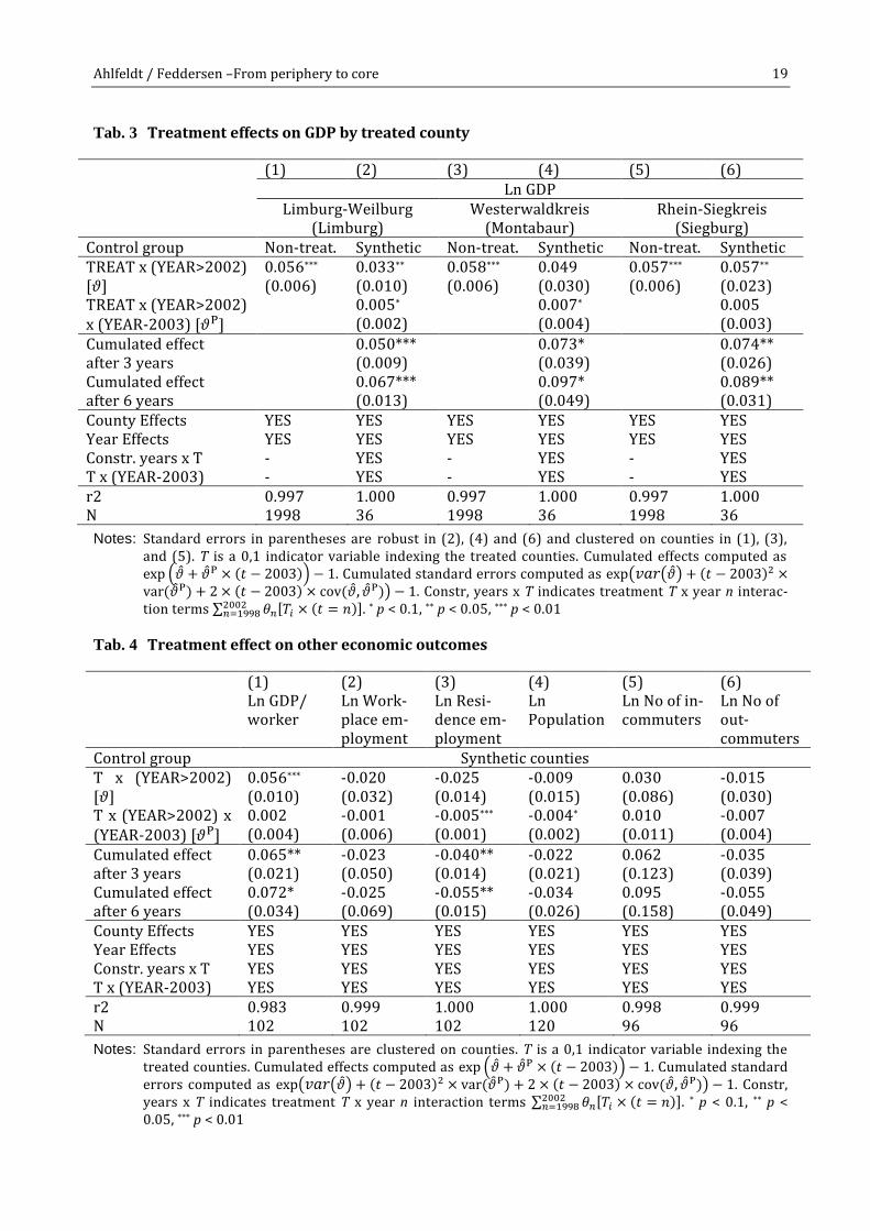
In Table 3 we replicate the least (1) and most (6) demanding models from Table 2 separately for
each of the treated counties. We find positive effects on each of the treated counties, which are
roughly within the range of the effects derived from the pooled models. After six years, each of the
treated counties exceeded its synthetic counterpart by about 7–10% in terms of GDP. Table 4, applies
the most demanding specification (comparison to synthetic control counties controlling for trends)
to different outcome measures. We find a positive and statistically significant effect on per-worker
GDP, which is roughly within the range of the GDP impact just discussed. Economic growth thus
seems to have come at least in part, if not entirely through, an increase in productivity (of the labor
force). We do not find positive and significant impacts on any other outcome measure.
Overall, the results of the econometric analysis support the key finding of the visual trend inspection
that the HSR increased the attractiveness of the locations close to the intermediate stations as places
to work, but not necessarily as places to live.
Ahlfeldt / Feddersen –From periphery to core 19
Tab. 3 Treatment effects on GDP by treated county
(1) (2) (3) (4) (5) (6) Ln GDP Limburg-Weilburg
(Limburg) Westerwaldkreis
(Montabaur) Rhein-Siegkreis
(Siegburg) Control group Non-treat. Synthetic Non-treat. Synthetic Non-treat. Synthetic TREAT x (YEAR>2002) [𝜗]
0.056*** (0.006)
0.033** (0.010)
0.058*** (0.006)
0.049 (0.030)
0.057*** (0.006)
0.057** (0.023)
TREAT x (YEAR>2002) x (YEAR-2003) [𝜗P]
0.005* (0.002)
0.007* (0.004)
0.005 (0.003)
Cumulated effect 0.050*** 0.073* 0.074** after 3 years (0.009) (0.039) (0.026) Cumulated effect 0.067*** 0.097* 0.089** after 6 years (0.013) (0.049) (0.031) County Effects YES YES YES YES YES YES Year Effects YES YES YES YES YES YES Constr. years x T - YES - YES - YES T x (YEAR-2003) - YES - YES - YES r2 0.997 1.000 0.997 1.000 0.997 1.000 N 1998 36 1998 36 1998 36
Notes: Standard errors in parentheses are robust in (2), (4) and (6) and clustered on counties in (1), (3), and (5). T is a 0,1 indicator variable indexing the treated counties. Cumulated effects computed as exp (�̂� + �̂�P × (𝑡 − 2003)) − 1. Cumulated standard errors computed as exp(𝑣𝑎𝑟(�̂�) + (𝑡 − 2003)2 ×var(�̂�P) + 2 × (𝑡 − 2003) × cov(�̂�, �̂�P)) − 1. Constr, years x T indicates treatment T x year n interac-tion terms ∑ 𝜃𝑛[𝑇𝑖 × (𝑡 = 𝑛)]2002
𝑛=1998 . * p < 0.1, ** p < 0.05, *** p < 0.01
Tab. 4 Treatment effect on other economic outcomes
(1) (2) (3) (4) (5) (6) Ln GDP/
worker Ln Work-place em-ployment
Ln Resi-dence em-ployment
Ln Population
Ln No of in-commuters
Ln No of out-commuters
Control group Synthetic counties T x (YEAR>2002) [𝜗]
0.056*** (0.010)
-0.020 (0.032)
-0.025 (0.014)
-0.009 (0.015)
0.030 (0.086)
-0.015 (0.030)
T x (YEAR>2002) x (YEAR-2003) [𝜗P]
0.002 (0.004)
-0.001 (0.006)
-0.005*** (0.001)
-0.004* (0.002)
0.010 (0.011)
-0.007 (0.004)
Cumulated effect 0.065** -0.023 -0.040** -0.022 0.062 -0.035 after 3 years (0.021) (0.050) (0.014) (0.021) (0.123) (0.039) Cumulated effect 0.072* -0.025 -0.055** -0.034 0.095 -0.055 after 6 years (0.034) (0.069) (0.015) (0.026) (0.158) (0.049) County Effects YES YES YES YES YES YES Year Effects YES YES YES YES YES YES Constr. years x T YES YES YES YES YES YES T x (YEAR-2003) YES YES YES YES YES YES r2 0.983 0.999 1.000 1.000 0.998 0.999 N 102 102 102 120 96 96
Notes: Standard errors in parentheses are clustered on counties. T is a 0,1 indicator variable indexing the treated counties. Cumulated effects computed as exp (�̂� + �̂�P × (𝑡 − 2003)) − 1. Cumulated standard errors computed as exp(𝑣𝑎𝑟(�̂�) + (𝑡 − 2003)2 × var(�̂�P) + 2 × (𝑡 − 2003) × cov(�̂�, �̂�P)) − 1. Constr, years x T indicates treatment T x year n interaction terms ∑ 𝜃𝑛[𝑇𝑖 × (𝑡 = 𝑛)]2002
𝑛=1998 . * p < 0.1, ** p < 0.05, *** p < 0.01
Ahlfeldt / Feddersen –From periphery to core 20
C – Falsification
As with any program evaluation the key identification challenge in our empirical exercise is to find a
credible counterfactual for the treated group. To ensure a valid comparison we have constructed a
synthetic control group which resembles the treated counties in terms of observable characteristics
and pre-treatment trends. In addition, we have made use of an econometric model that controls for
heterogeneity in pre-trends between the treated and the control counties. We argue that this degree
of sophistication helps to reduce the risk of erroneously attributing different macroeconomic trends
that result from differences between the groups of treated and control counties to the HRS. But we
acknowledge that there is, ultimately, no formal way of affirming that the true counterfactual trend
has been established. What can be done is to evaluate the likelihood that our empirical design reveals
a treatment effect where, in effect, there is no treatment.
We begin a with a classic “placebo” study. We apply our empirical strategy to an HSR which was con-
sidered during the planning stage but never built. The track would also have had three intermediate
stops in each of the involved federal states and would have passed through the economically and
politically relevant cities of Bonn (the former federal capital located in North Rhine-Westphalia),
Koblenz (the largest city in northern Rhineland-Palatinate) and Wiesbaden (the state capital of Hes-
se). The results are easily summarized. The mean treatment effect on the GDP across the three cities
is near to and not statistically different from zero in all specifications. The separate treatment esti-
mates by treated county produce significant estimates with mixed signs in the naïve DD specification,
but no significant cumulative effects using synthetic counties as comparisons (although Wiesbaden
has a near to 10% significance level positive long-run effect). We don’t find any significant effect of
the other outcome measures either, although there are large and positive point estimates for per-
worker GDP (but even larger standard errors).
Focusing on GDP as an outcome measure, we next take the placebo analysis one step further. We run
a series of 1,000 similar placebo models for randomly designed HSR. In each placebo model we first
randomly select one county as one endpoint of the line (the placebo Cologne). Second, we randomly
select another endpoint (the placebo Frankfurt) from all counties within a 140–180km range (in
terms of straight-line distances) of the first endpoint (the distance between Cologne and Frankfurt is
160km). Third, we pick the three counties whose economic center (the largest city) is closest to a
straight line connecting the two endpoints and define them as the treated counties (the placebo in-
termediate stops). Fourth, we create synthetic comparison counties for each of the placebo treated
Ahlfeldt / Feddersen –From periphery to core 21
counties according to our standard procedure. Fifth, we estimate the naïve DD model (Table 2, col-
umn 3 model, which uses all non-treated control counties and does not control for trends) as well as
our preferred model (Table 2, column 6 model, which uses synthetic control counties and controls
for trends) and save the point estimates and significance levels. Of the 1,000 placebos tests 8.4%
(24%) deliver significant treatment effects after six years using our preferred (naïve) DD model.
5.6% (8.2%) iterations resulted in treatment effects that were significant (at the 10% level) and at
least as large as our benchmark estimates. The mean of the point estimate is very close to zero. Nota-
bly, the standard deviation across placebo point estimates with 8.6% (5.4%) is relatively large com-
pared to our 8.4% (5.7%) treatment estimate.
We conclude that it is unlikely that our empirical specification delivers significant treatment effects
that are spurious. For further details on the empirical results of the placebo tests we refer to the web
appendix (section 3).
4 Agglomeration effects
Given the results presented so far it seems fair to conclude that the HSR has had a positive impact on
the economies of the counties of the intermediate stops. This impact is in line with the idea that an
increase in (market) accessibility should increase the attractiveness of a location as a place of pro-
duction. In the next step we seek to model the change in accessibility pattern induced by the HSR
more fully to gain insights into the strength and the spatial scope of agglomeration forces.
A – Empirical strategy
In our baseline empirical model we assume that the output in county i in year t denoted by 𝑄𝑖𝑡 de-
pends on effective density 𝐷𝑖𝑡 as well as arbitrary county effects 𝑐𝑖 and year effects dt.
ln(𝑄𝑖𝑡) = 𝛿1 ln(𝐷𝑖𝑡) + 𝑐𝑖 + 𝑑𝑡 + 휀𝑖𝑡 (4-1)
, where 𝛿1 is the elasticity of output with respect to effective density for marginal changes in D and 휀𝑖𝑡
is a random error. We hypothesize that, all else equal, access to a larger economic mass should in-
crease firm productivity and lead to higher economic output. We model effective density as a func-
tion of output across all counties j within reach and, thus, assume a black-box agglomeration force
that depends on the productivity of all non-land inputs. Specifically, we allow for bilateral productivi-
ty externalities between all counties, assuming that the spillover effect declines exponentially in a

Ahlfeldt / Feddersen –From periphery to core 22
measure of effective distance Eij between regions i and j, which takes into account the availability of
transport infrastructure. Our measure of effective density thus takes the market potential form
(Harris, 1954), which is popular in the theoretical (Fujita and Ogawa, 1982; Lucas and Rossi-
Hansberg, 2002) and empirical (Ahlfeldt, et al., 2015; Ahlfeldt and Wendland, 2013) agglomeration
economics literature. Similar measures have been used in the empirical NEG literature (Hanson,
2005; Redding and Sturm, 2008).
𝐷𝑖𝑡 = ∑ 𝑄𝑗𝑒−𝛿2𝐸𝑖𝑗
𝑗 (4-2)
, where 𝛿2>0 determines the rate of spatial decay of the productivity effect in effective distance be-
tween two regions i and j.11 The strength of the market potential formulation is that it effectively al-
lows the productivity effect of spatial externalities to vary in effective distance to the surrounding
economic mass without imposing arbitrary discrete classifications. Instead of assuming that exter-
nalities operate within the administrative borders of a region or contiguous groups of regions, our
measure of effective density also accounts for externalities across such borders.
Estimating the parameters of interest 𝛿1 and 𝛿2 is challenging for a variety of reasons. Firstly, it is
difficult to control for all location factors subsumed in ci , which impact on productivity and are po-
tentially correlated with the agglomerations measure. Secondly, there is a mechanical endogeneity
problem because the dependent variable output (Qit) also appears in the market potential of regions
i=j. Unobserved shocks to output can therefore lead to a spurious correlation between the outcome
measure and effective density. The problem is non-trivial given that internal effective distance Eij=i is
typically short so that the Qij=i receives a relatively high weight. Thirdly, it is likely that shocks to out-
puts are spatially correlated so that the same problem also applies to nearby areas i and j.
The first problem can be addressed by estimating equation (4-1) in differences so that unobserved
time-invariant location factors are differentiated out as, for example, in Hanson (2005). Informed by
the program evaluation results, we take long differences over the construction period from 1998 to
2002 in our baseline estimation, but we consider alternative end dates in an alternative specification.
The second problem, in principle, can be mitigated by aggregating right-hand side areas j to larger
11 Our internal effective distance Eij=i depends on the land area of county i so that our measure corresponds to a
standard density measure for the within county externalities.
Ahlfeldt / Feddersen –From periphery to core 23
spatial units (e.g., Hanson, 2005) or replacing Qij=i with imputed values (Ahlfeldt and Wendland,
2013). Both strategies come at the cost of losing information. The third problem is even more diffi-
cult to address since shocks to output at nearby regions are likely correlated not only in levels but
also in trends.
Our empirical strategy addresses the abovementioned problems by exploiting the variation in bilat-
eral transport times created by the HSR. We set the output levels at all locations j to 𝑄𝑗𝑡=1998 in both
periods, so that the identification comes exclusively from changes in effective distance. Our estima-
tion equation thus takes the following form:
ln(𝑄𝑖,𝑡=2002) − ln(𝑄𝑖,𝑡=1998) = 𝛿0 + δ1
[ ln (∑ 𝑄𝑗,𝑡=1998𝑒
−𝛿2𝐸𝑖𝑗,𝑡=2002
𝑗)
− ln (∑ 𝑄𝑗,𝑡=1998𝑒−𝛿2𝐸𝑖𝑗,𝑡=1998
𝑗)]
+ ∆휀𝑖 (4-3)
We stress that this specification differs from a conventional first-difference approach in that the first-
difference in the market potential is driven by changes in the travel time, but not output. Specifica-
tion (4-3) is estimated using a non-linear least squares estimator to simultaneously determine both
parameters of interest (δ1 and δ2). With the estimated parameters it is then possible to express the
effect of an increase in economic mass at j by one unit of initial market potential of county i on the
outcome of county i as a function of the bilateral effective distance:
𝜕log (𝑄𝑖)
𝜕(𝑄𝑗)× (∑ 𝑄𝑗𝑒
−𝛿2𝐸𝑖𝑗
𝑗) = δ1̂exp (−𝛿2̂𝐸𝑖𝑗)
(4-4)
Similar increases in economic mass are expected to benefit a county more if it happens in a county
within a shorter effective distance.
We consider several alterations of specification (4-3) for the purposes of validation, falsification, and
evaluation of robustness. We estimate equation (4-3) using the GVA in various industry sectors as an
outcome variable. We consider a grid search over a large parameter space (𝛿1, 𝛿2) to evaluate wheth-
er the agglomeration and spillover parameters are credibly separately identified. We contrast our
results with those derived from a market potential specification that allows for more flexibility in the
spatial decay. We allow for trends correlated with initial sectorial composition, workforce qualifica-
tion, and exposure to agglomeration. We also control for trends pre-existing the construction of the
HSR and explore the temporal pattern of adjustment using an alternative panel specification. Im-

Ahlfeldt / Feddersen –From periphery to core 24
portantly, we use instrumental variables to restrict the identifying variation to the portion that is not
only exogenous with respect to the timing, but also with respect to the routing of the HSR. For falsifi-
cation, we make use of the placebo HSR, which was considered but never built, and public sector GVA
as an outcome, which we expect not to respond to the HSR, at least in the short run. Finally, we repli-
cate the main stages of the analysis using per-worker GDP as a dependent variable to connect more
closely to the literature on the productivity effects of density. In this alternative specification we will
also control for changes in the industry sector structure and workforce qualification to address selec-
tion effects.
B – Approximation of effective distance
To implement the empirical strategy laid out above we require empirical approximations of the bi-
lateral travel costs between each pair of counties in the study area, the effective distance. To compute
our measures of effective distance we make use of a Geographic Information System (GIS) and the
information on transport infrastructure displayed in Figure 1. In connecting two counties we refer to
the largest cities within the pair of counties as the respective centers of economic mass (the black
dots in Figure 1). In computing the effective distance we assume that transport costs are incurred
exclusively in terms of travel time and that route choice is based on travel time minimization.
To solve for the least-cost matrix connecting all potential origins and destinations we assign travel
times to each fraction of the transport network, which are based on the network distance and the
following speeds: 160km/h for HSR, which is roughly in line with the 70min journey along the
180km Cologne-Frankfurt HSR line; 80km/h for conventional rail, which is roughly in line with the
140min journey along the 205km conventional rail line; 100km/h for motorways and 80km/h on the
other primary roads. In combining these transport modes we experiment with different procedures.
In our benchmark cost matrix we allow travellers to change from roads to conventional rail in any
city (they all have rail stations) and from any mode to HSR at the dedicated HSR stations (white cir-
cles in Figure 1) if in the respective period HSR is available. For robustness checks we compute travel
times according to two alternative decision rules. In one version travellers can choose either the au-
tomobile or rail, including HSR if available, but they are not allowed to switch mode during a journey.
In a further alternative we eliminate the automobile altogether. Since the automobile is typically the
more competitive mode the resulting change in travel time reflects an upper bound of the true acces-
sibility gain.
Ahlfeldt / Feddersen –From periphery to core 25
In each case, we approximate the average internal travel time within a region i=j as the travel time
that corresponds to a journey at 80km/h (primary road) along a distance that corresponds to two-
thirds of the radius of a circle with the same surface area.
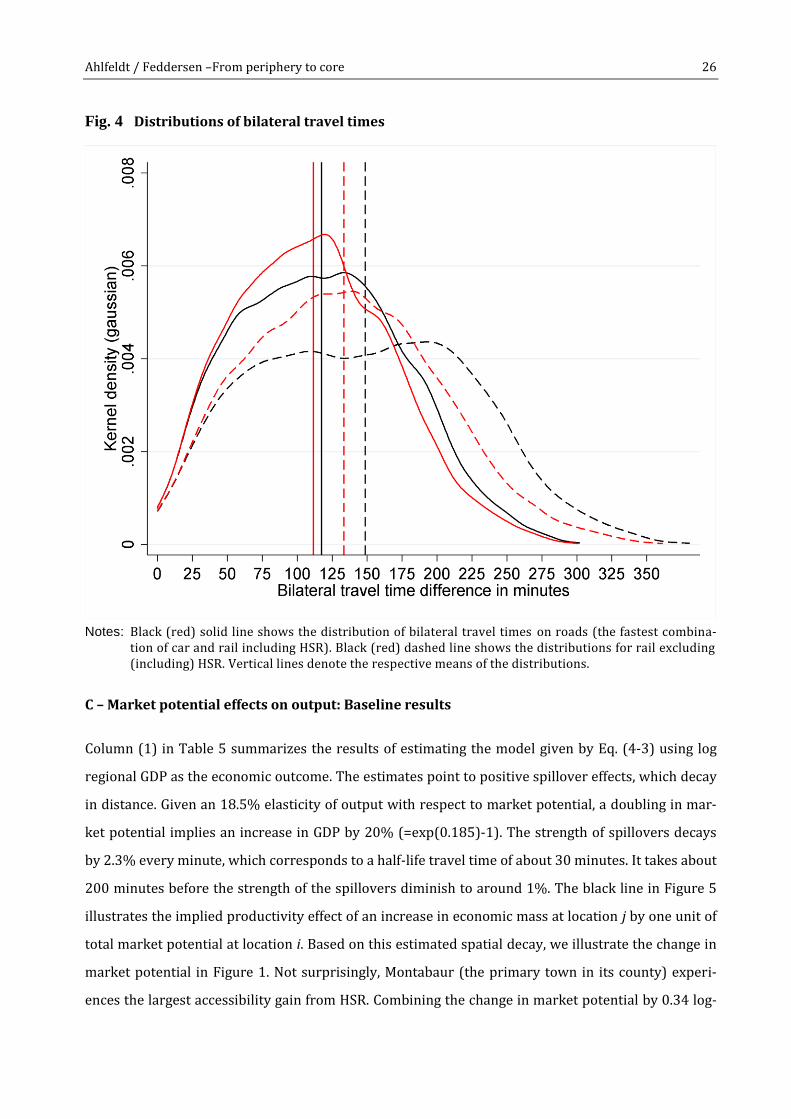
Figure 4 summarizes the distribution of travel times across the 1152=13,225 county pairs in the situ-
ations with and without HRS according to the baseline decision rule and the rail-only alternative.
Evidently, the introduction of HSR had a significant impact on the competitiveness of the rail network
as reflected by the major shift in the distribution of rail travel times (dashed lines) toward the distri-
bution of road travel times (black solid line). Prior to HSR, the road network offered faster connec-
tions for almost all county pairs so that the road travel time matrix effectively describes the least-
cost matrix (black solid lines). As expected, adding HSR as a potential mode that can be combined
with the automobile reduces travel times significantly on a number of routes, especially on those that
would otherwise take 50min or more (red solid line).
Ahlfeldt / Feddersen –From periphery to core 26
Fig. 4 Distributions of bilateral travel times
Notes: Black (red) solid line shows the distribution of bilateral travel times on roads (the fastest combina-
tion of car and rail including HSR). Black (red) dashed line shows the distributions for rail excluding (including) HSR. Vertical lines denote the respective means of the distributions.
C – Market potential effects on output: Baseline results
Column (1) in Table 5 summarizes the results of estimating the model given by Eq. (4-3) using log
regional GDP as the economic outcome. The estimates point to positive spillover effects, which decay
in distance. Given an 18.5% elasticity of output with respect to market potential, a doubling in mar-
ket potential implies an increase in GDP by 20% (=exp(0.185)-1). The strength of spillovers decays
by 2.3% every minute, which corresponds to a half-life travel time of about 30 minutes. It takes about
200 minutes before the strength of the spillovers diminish to around 1%. The black line in Figure 5
illustrates the implied productivity effect of an increase in economic mass at location j by one unit of
total market potential at location i. Based on this estimated spatial decay, we illustrate the change in
market potential in Figure 1. Not surprisingly, Montabaur (the primary town in its county) experi-
ences the largest accessibility gain from HSR. Combining the change in market potential by 0.34 log-
Ahlfeldt / Feddersen –From periphery to core 27
points with the estimated market potential elasticity the predicted increase in GDP for Montabaur is
about 6%, which is close to the cumulated effect after three years detected in the program evaluation
section.
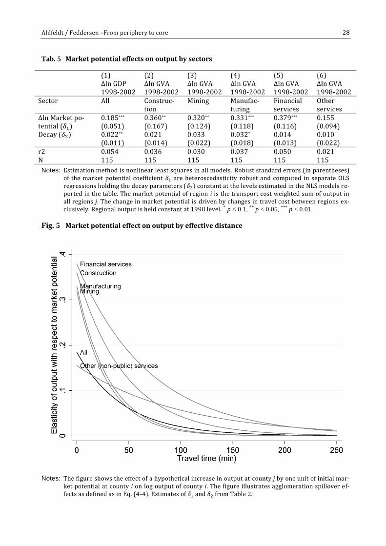
The remaining columns in Table 5 present results according to Eq. (4-3) replacing regional GDP with
the GVA of various industry sectors as the outcome variable. The estimated spillover effects are visu-
alized in Figure 5 as gray lines. The estimates are generally within the range of column (1). For some
sectors the parameters are, however, estimated less precisely. The results also suggest that the mar-
ket potential elasticity estimated in column (1) is brought down somewhat by sectors that are appar-
ently less susceptible to agglomeration benefits, namely services other than financial services. For
construction, mining, manufacturing, and financial services the elasticity of output with respect to
market potential is relatively large.
As the HSR line is used exclusively for passenger transport, we expect to capture Marshallian exter-
nalities related to human interactions. Candidates are knowledge spillovers due to formal and infor-
mal meetings, improved labor market access and matching, as well as improved access to intermedi-
ated goods and consumer markets to the extent that the ease of communication reduces transaction
costs but not freight costs. Our results are thus principally comparable to Ahlfeldt et al. (2015) and
Ahlfeldt and Wendland (2013) who have estimated the effects of spillovers on productivity from
within-city variation. These studies have found spillover effects that are significantly more localized.
The spillover effect in these studies decay to near to zero within about half a kilometer, which is in
line with Arzaghi and Henderson (2008) who also focus on within-city variation. Compared to these
studies the lower spatial decay suggests that we are capturing different types of spatial externalities.
While the steep spillover decay in the within-city studies points to a dominating role of face-to-face
contacts that purposely or accidently happen at high frequency in the immediate neighborhood
(Storper and Venables, 2004), our results suggest that the HSR effects operate at an intermediate
range and through the benefits of shared inputs and labor pools, labor market matching or increases
in consumer and producer market access. This interpretation is also in line with the significantly
lower spatial decay found in an empirical NEG studies with an emphasis on trade costs (Hanson,
2005).
Ahlfeldt / Feddersen –From periphery to core 28
Tab. 5 Market potential effects on output by sectors
(1) (2) (3) (4) (5) (6) Δln GDP
1998-2002 Δln GVA 1998-2002
Δln GVA 1998-2002
Δln GVA 1998-2002
Δln GVA 1998-2002
Δln GVA 1998-2002
Sector All Construc-tion
Mining Manufac-turing
Financial services
Other services
Δln Market po-tential (𝛿1)
0.185*** (0.051)
0.360** (0.167)
0.320** (0.124)
0.331*** (0.118)
0.379*** (0.116)
0.155 (0.094)
Decay (𝛿2) 0.022** 0.021 0.033 0.032* 0.014 0.010 (0.011) (0.014) (0.022) (0.018) (0.013) (0.022) r2 0.054 0.036 0.030 0.037 0.050 0.021 N 115 115 115 115 115 115
Notes: Estimation method is nonlinear least squares in all models. Robust standard errors (in parentheses) of the market potential coefficient 𝛿1 are heteroscedasticity robust and computed in separate OLS regressions holding the decay parameters (𝛿2) constant at the levels estimated in the NLS models re-ported in the table. The market potential of region i is the transport cost weighted sum of output in all regions j. The change in market potential is driven by changes in travel cost between regions ex-clusively. Regional output is held constant at 1998 level. * p < 0.1,
** p < 0.05,
*** p < 0.01.
Fig. 5 Market potential effect on output by effective distance
Notes: The figure shows the effect of a hypothetical increase in output at county j by one unit of initial mar-
ket potential at county i on log output of county i. The figure illustrates agglomeration spillover ef-fects as defined as in Eq. (4-4). Estimates of 𝛿1 and 𝛿2 from Table 2.
Ahlfeldt / Feddersen –From periphery to core 29
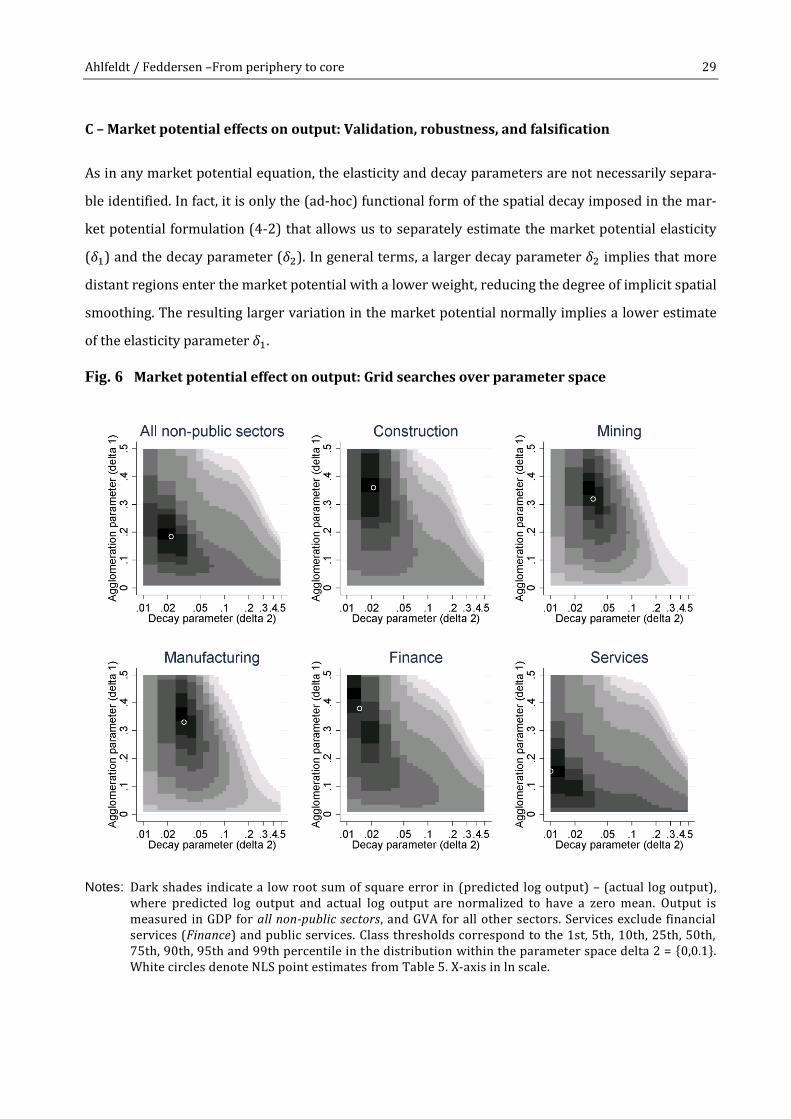
C – Market potential effects on output: Validation, robustness, and falsification
As in any market potential equation, the elasticity and decay parameters are not necessarily separa-
ble identified. In fact, it is only the (ad-hoc) functional form of the spatial decay imposed in the mar-
ket potential formulation (4-2) that allows us to separately estimate the market potential elasticity
(𝛿1) and the decay parameter (𝛿2). In general terms, a larger decay parameter 𝛿2 implies that more
distant regions enter the market potential with a lower weight, reducing the degree of implicit spatial
smoothing. The resulting larger variation in the market potential normally implies a lower estimate
of the elasticity parameter 𝛿1.
Fig. 6 Market potential effect on output: Grid searches over parameter space
Notes: Dark shades indicate a low root sum of square error in (predicted log output) – (actual log output),
where predicted log output and actual log output are normalized to have a zero mean. Output is measured in GDP for all non-public sectors, and GVA for all other sectors. Services exclude financial services (Finance) and public services. Class thresholds correspond to the 1st, 5th, 10th, 25th, 50th, 75th, 90th, 95th and 99th percentile in the distribution within the parameter space delta 2 = {0,0.1}. White circles denote NLS point estimates from Table 5. X-axis in ln scale.
Ahlfeldt / Feddersen –From periphery to core 30
As there could be multiple combinations of these critical parameters that fit the data we have run a
grid-search over 500 possible values of 𝛿1 and 𝛿2(0.001 to 0.5) resulting in 250,000 parameter com-
binations for each of the models reported in Table 5. For each parameter combination we compute
the root sum of the square deviations between the observed and predicted changes in regional out-
put. As illustrated in Figure 6, we find relatively clearly defined global minima, supporting the para-
metric estimates presented in Table 5 and Figure 5.
In Table 6 we present a series of alterations of the baseline model in column (1) of Table 5. We fix the
decay parameter to the value estimated in the baseline model (Table 5, column 1) so the market po-
tential elasticity remains comparable across alternative models. In columns (1–3) we control for
trends that may be correlated with but are economically unrelated to the change in market potential
and potentially confound the estimates. The purpose of these models is, thus, similar to the matching
on observables we imposed in the construction of synthetic counties in the program evaluation sec-
tion. In model (4) we additionally control for the (1992 to 1997) pre-trend in log GDP to account for
the possibility that unobserved county characteristics determine long-run growth trends.12 This con-
trol serves a similar purpose to the matching on pre-trends in the construction of the synthetic coun-
ties and the control for heterogeneity in pre-trends in the program evaluation DD model. The market
potential elasticity decreases somewhat but remains significant and within the range of the baseline
estimate.
In model (5) we exploit that the timing and the routing of the HSR line can be assumed to be exoge-
nous for the intermediate stops (Limburg, Montabaur, Siegburg) while “only” the timing (and not the
routing) is exogenous for the endpoints Cologne and Frankfurt. To restrict the variation in change in
market potential to the fraction that is most plausibly exogenous we instrument the change in mar-
ket potential with three indicator variables, each denoting one of the counties in which the interme-
diate stops are located. The market potential elasticity remains significant, but decreases somewhat
further to about 12.5%.
In model (6) we use GVA in the public sector instead of total GDP as the left-hand side measure of
output. We view this model as a placebo test because the spatial distribution of this sector is unlikely
12 We take the lagged log GDP long-difference over the period 1992–1997 instead of 1992–1998 to avoid a
mechanical endogeneity problem that would arise if the 1998 log GDP was entered on both sides of the
equation.
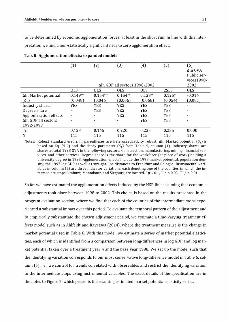
Ahlfeldt / Feddersen –From periphery to core 31
to be determined by economic agglomeration forces, at least in the short run. In line with this inter-
pretation we find a non-statistically significant near to zero agglomeration effect.
Tab. 6 Agglomeration effects: expanded models
(1) (2) (3) (4) (5) (6)
Δln GDP all sectors 1998-2002
Δln GVA Public ser-vices1998-2002
OLS OLS OLS OLS 2SLS OLS Δln Market potential (𝛿1)
0.149*** (0.048)
0.154*** (0.046)
0.154** (0.066)
0.138** (0.068)
0.125** (0.054)
-0.014 (0.081)
Industry shares YES YES YES YES YES - Degree share - YES YES YES YES - Agglomeration effects - - YES YES YES - Δln GDP all sectors 1992-1997
- - - YES YES -
r2 0.123 0.145 0.220 0.235 0.235 0.000 N 115 115 115 115 115 115
Notes: Robust standard errors in parentheses are heteroscedasticity robust. Δln Market potential (𝛿1) is based on Eq. (4-2) and the decay parameter (𝛿1) from Table 5, column (1). Industry shares are shares at total 1998 GVA in the following sectors: Construction, manufacturing, mining, financial ser-vices, and other services. Degree share is the share for the workforce (at place of work) holding a university degree in 1998. Agglomeration effects include the 1998 market potential, population den-sity, the 1997 log GDP as well as straight-line distances to Frankfurt and Cologne. Instrumental vari-ables in column (5) are three indicator variations, each denoting one of the counties in which the in-termediate stops Limburg, Montabaur, and Siegburg are located. * p < 0.1,
** p < 0.05,
*** p < 0.01.
So far we have estimated the agglomeration effects induced by the HSR line assuming that economic
adjustments took place between 1998 to 2002. This choice is based on the results presented in the
program evaluation section, where we find that each of the counties of the intermediate stops expe-
rienced a substantial impact over this period. To evaluate the temporal pattern of the adjustment and
to empirically substantiate the chosen adjustment period, we estimate a time-varying treatment ef-
fects model such as in Ahlfeldt and Kavetsos (2014), where the treatment measure is the change in
market potential used in Table 6. With this model, we estimate a series of market potential elastici-
ties, each of which is identified from a comparison between long-differences in log GDP and log mar-
ket potential taken over a treatment year n and the base year 1998. We set up the model such that
the identifying variation corresponds to our most conservative long-difference model in Table 6, col-
umn (5), i.e., we control for trends correlated with observables and restrict the identifying variation
to the intermediate stops using instrumental variables. The exact details of the specification are in
the notes to Figure 7, which presents the resulting estimated market potential elasticity series.

Ahlfeldt / Feddersen –From periphery to core 32
Fig. 7 Market potential elasticity: Time-varying estimates
Notes: The figure is based on the following panel specification: ln(𝑄𝑖𝑡) = ∑ [𝛿1,𝑛∆ ln(𝐷𝑖) × (𝑡 = 𝑛)]𝑛≠1998 +
𝑋𝑖𝑡𝑏𝑡 + 𝑐𝑖 + 𝑑𝑡 + 휀𝑖𝑡. where Qit is the output measured as GDP of county i in year t, n indexes treat-ment years from 1992 to 2009, excluding the base year 1998, ∆ ln(𝐷𝑖) is the change in market poten-tial assuming the decay parameter estimated in Table 5, column (1), Xit is a vector year effects inter-acted with a vector of the following variables: industry shares at total 1998 GVA (construction, man-ufacturing, mining, financial services, and other non-public services), the share of the workforce (at place of work) holding a university degree in 1998, the 1998 market potential, population density, the 1997 log GDP as well as straight-line distances to Frankfurt and Cologne. 𝑏𝑡 is a matrix of coeffi-cients for each variable-year combination. 𝑐𝑖 and 𝑑𝑡 are county and year effects as in equation (4-1). We instrument the vector of change in market potential × year interaction terms ∆ ln(𝐷𝑖) × (𝑡 = 𝑛) using a full set of interaction terms between year effects and three indicator variations, each deno t-ing one of the counties in which the intermediate stops Limburg, Montabaur, and Siegburg are locat-ed. Black dots represent point estimates of 𝛿1,𝑛 and the gray shaded area denotes the 95% confidence intervals (standard errors clustered on the counties). Vertical dashed lines frame the period over which long-difference are taken in Tables 5 and 6. The upper horizontal dashed lines indicates the market potential elasticity estimated in Tables 6, column (5) model, which in terms of the identifying variation is comparable to the model presented.
As expected, we find no significant response in the spatial distribution of economic activity to the
market potential shock for treatment years n<1998, while the estimates of the market potential elas-
ticity converge to the estimate in Tables 6, column (5) relatively quickly for treatment years n>1998.

Ahlfeldt / Feddersen –From periphery to core 33
By 2000, still in anticipation of the opening of the line in 2002, the spatial economy seems to have
adjusted to the market potential shock as the time-varying estimates of the elasticity then remain
relatively stable for a number of consecutive years. This pattern is suggestive of an impact of the HSR
on the level, but not the trend of economic activity. In 2006, however, we observe a further relative
shift in economic activity in regions which benefited from the HSR. Looking at the overall trend in the
economic adjustment, this shift seems somewhat detached from the market potential shock, and it
remains ultimately difficult to assert whether or not this shift is causally related to the HSR.
We have conducted a number of further alterations of our baseline model, which we briefly discuss
in the remainder of this subsection. A more detailed discussion can be found in the appendix.
The exponential functional form of the spatial decay in spillovers, while popular in the theoretical
and empirical literature (e.g., Ahlfeldt, et al., 2015; Fujita and Ogawa, 1982; Lucas and Rossi-
Hansberg, 2002), is ad-hoc and other functional forms are theoretically imaginable. We have esti-
mated an alternative version of our benchmark model in which the market potential is captured as
the total GDP within several mutually exclusive 20-minute travel time bins (e.g., 0–20 min, 20–40
min, etc.). For each travel time bin a separate market potential elasticity is estimated, thus allowing
for a more flexible pattern in the spatial decay. When comparing the predicted effects of the change
in market potential on GDP in this alternative model to our baseline model, we find an approximately
linear relationship, suggesting that our results are not driven by an inappropriate functional form of
the spatial decay (see appendix 3-A).
We have experimented with alternative travel choice models underlying the construction of travel
times. In one alternative choice model, we disallow switching from train to automobile or vice versa
along a journey. In another alternative choice model, we disallow the use of the automobile altogeth-
er. The results remain qualitatively unchanged and quantitatively within the range of the results pre-
sented here (see appendix 3-B).
We have also experimented with alternative instrumental variables to restrict the identification to
variation in the change in market potential to the fraction that arises from the intermediate transport
stations. In particular, we consider the log straight-line distance to Montabaur as well as indictor
variables for the counties of the intermediate stops as well as the adjacent counties as alternatives.
The results remain close to those reported in Table 6 (see appendix 3-C).
Ahlfeldt / Feddersen –From periphery to core 34
Finally, we have also replicated the main stages of our analysis replacing the actual HSR with the
considered but never built placebo HSR, which we introduced in the previous section. We find no
robust evidence of HSR effects in this falsification exercise (see appendix 3-D).
D – Market potential effects on productivity
As discussed in the introduction a large literature has analyzed agglomeration effects by regressing a
measure of productivity against a measure of density. In order to connect to this literature and to
assess to which extent the market potential (effective density) effect on GDP discussed above is at-
tributable to an increase in productivity of the labor force (rather than an expansion of the labor
force), we replicate our baseline model using the ratio of GDP over the total employment (at work-
place) as a dependent variable. The empirical specification used shared similarities with the nominal
wage equation estimated in the NEG literature (e.g., Hanson, 2005) . In Table 7 we present the results
of three OLS (1–3) and three 2SLS (4–6) estimations. In each case, we present unconditional correla-
tions between per-worker GDP growth and change in log market potential, a version using the same
controls as in Table 6, column (4), and one version where we additionally account for changes in the
industry structure and the skill composition of the workforce. The instrumental variables used are
the same as in Table 6, column (5).
The preferred results in columns (2) and (5) suggest that the increase we find in GDP is driven by an
increase in worker productivity, rather than an expansion of the workforce, as the estimated elastici-
ty is within the range of the models in Table 6. In comparing these results to the literature on the
productivity effects of density it is important to acknowledge that unlike conventional density
measures, our market potential takes into account the economic activity in surrounding regions, al-
beit with a lower weight. As a measure of effective density the market potential therefore introduces
a spatial autocorrelation, which reduces variation in effective density across counties. It turns out
that the standard deviation in the 1998 log market potential across counties in our data is almost
three times the standard deviation in the 1998 log employment density. Our elasticity of productivity
with respect to effective density is, therefore, not directly comparable to the majority of estimates in
the agglomeration economics literature as a 1% increase in market potential, on average, implies a
much larger percentage increase in density. Normalized by the log ratio of the standard deviations of
effective density (market potential) over density (employment per area) our results imply a 3.8%
elasticity of productivity with respect to employment density, which is close to previous estimates
derived from cross-sectional research designs (e.g., Ciccone, 2002; Ciccone and Hall, 1996).
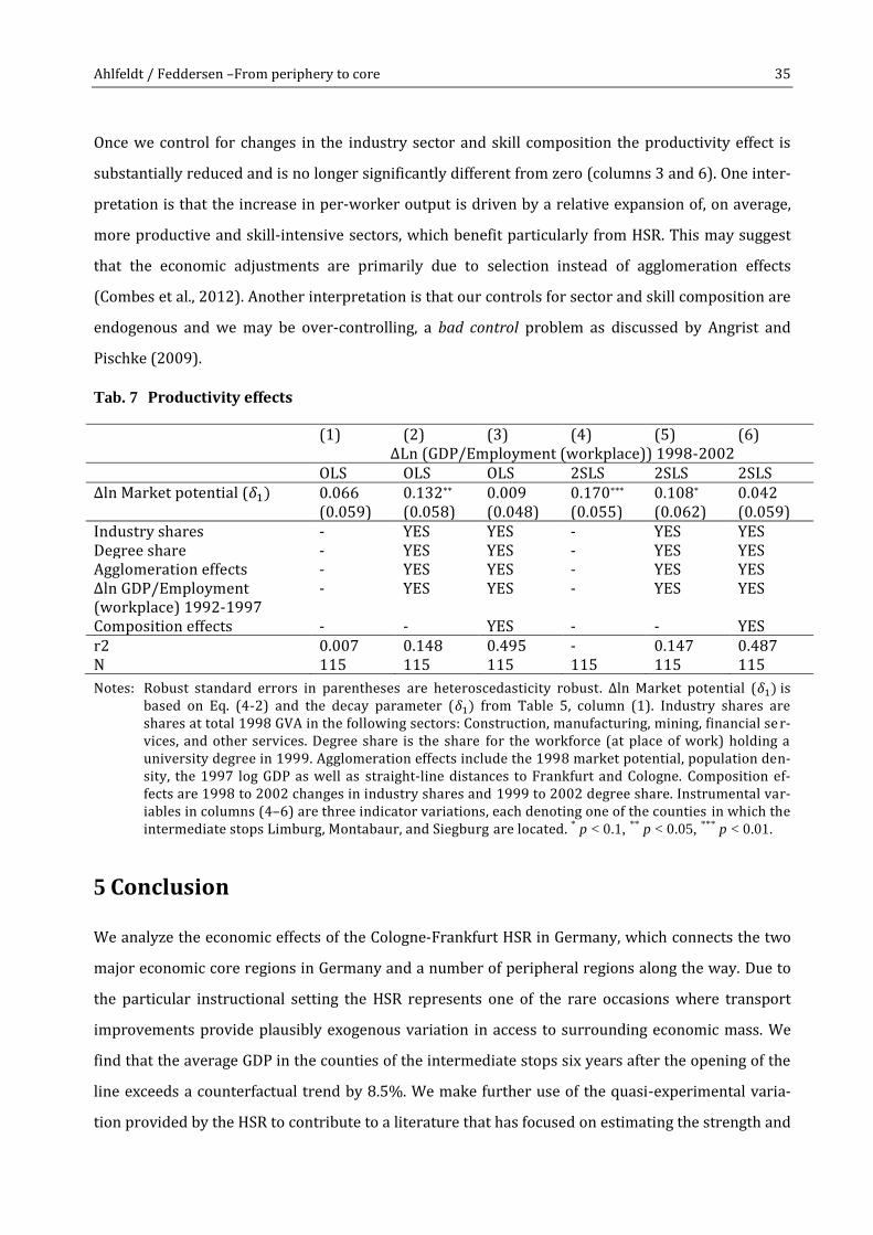
Ahlfeldt / Feddersen –From periphery to core 35
Once we control for changes in the industry sector and skill composition the productivity effect is
substantially reduced and is no longer significantly different from zero (columns 3 and 6). One inter-
pretation is that the increase in per-worker output is driven by a relative expansion of, on average,
more productive and skill-intensive sectors, which benefit particularly from HSR. This may suggest
that the economic adjustments are primarily due to selection instead of agglomeration effects
(Combes et al., 2012). Another interpretation is that our controls for sector and skill composition are
endogenous and we may be over-controlling, a bad control problem as discussed by Angrist and
Pischke (2009).
Tab. 7 Productivity effects
(1) (2) (3) (4) (5) (6) ∆Ln (GDP/Employment (workplace)) 1998-2002 OLS OLS OLS 2SLS 2SLS 2SLS Δln Market potential (𝛿1) 0.066
(0.059) 0.132** (0.058)
0.009 (0.048)
0.170*** (0.055)
0.108* (0.062)
0.042 (0.059)
Industry shares - YES YES - YES YES Degree share - YES YES - YES YES Agglomeration effects - YES YES - YES YES Δln GDP/Employment (workplace) 1992-1997
- YES YES - YES YES
Composition effects - - YES - - YES r2 0.007 0.148 0.495 - 0.147 0.487 N 115 115 115 115 115 115
Notes: Robust standard errors in parentheses are heteroscedasticity robust. Δln Market potential (𝛿1) is based on Eq. (4-2) and the decay parameter (𝛿1) from Table 5, column (1). Industry shares are shares at total 1998 GVA in the following sectors: Construction, manufacturing, mining, financial se r-vices, and other services. Degree share is the share for the workforce (at place of work) holding a university degree in 1999. Agglomeration effects include the 1998 market potential, population den-sity, the 1997 log GDP as well as straight-line distances to Frankfurt and Cologne. Composition ef-fects are 1998 to 2002 changes in industry shares and 1999 to 2002 degree share. Instrumental var-iables in columns (4–6) are three indicator variations, each denoting one of the counties in which the intermediate stops Limburg, Montabaur, and Siegburg are located. * p < 0.1,
** p < 0.05,
*** p < 0.01.
5 Conclusion
We analyze the economic effects of the Cologne-Frankfurt HSR in Germany, which connects the two
major economic core regions in Germany and a number of peripheral regions along the way. Due to
the particular instructional setting the HSR represents one of the rare occasions where transport
improvements provide plausibly exogenous variation in access to surrounding economic mass. We
find that the average GDP in the counties of the intermediate stops six years after the opening of the
line exceeds a counterfactual trend by 8.5%. We make further use of the quasi-experimental varia-
tion provided by the HSR to contribute to a literature that has focused on estimating the strength and
Ahlfeldt / Feddersen –From periphery to core 36
scope spatial scope of agglomeration effects. We find an elasticity of output with respect to effective
density, i.e., market potential, of about 12.5% in our most conservative model. Our results further
imply an elasticity of productivity with respect to density of 3.8%, which is well within the range of
existing cross-sectional estimates. The strength of spillovers halves every 30 minutes of travel time
and is near to zero after about 200 minutes. The spillovers we detect are significantly less localized
than in previous studies that have identified similar spillover effects from within-city variation, but
more localized than those found in the empirical NEG literature with an emphasis on trade cost. The
benefits HSR has delivered to the peripheral regions operate through knowledge diffusion and labor
market pooling and the effects of improved access to intermediated goods and consumer markets to
the extent that the ease of communication reduces transaction costs, and thus, Marshallian externali-
ties (Marshall, 1920). Our results complement recent evidence suggesting that improved transport
linkages can benefit core regions at the expense of peripheral regions through a trade channel (Faber,
2014).

Ahlfeldt / Feddersen –From periphery to core 37
Literature
Abadie, A., and Gardeazabal, J. (2003). The economic costs of conflict: A case study of the basque country. American Economic Review, 93(1), 113-132.
Ahlfeldt, G. M., and Kavetsos, G. (2014). Form or function? The impact of new sports stadia on property prices in london. Journal of the Royal Statistical Society A, 177(1), 169-190.
Ahlfeldt, G. M., Redding, S. J., Sturm, D. M., and Wolf, N. (2015). The economics of density: Evidence from the berlin wall. Econometrica, forthcoming.
Ahlfeldt, G. M., and Wendland, N. (2013). How polycentric is a monocentric city? Centers, spillovers and hysteresis. Journal of Economic Geography, 13(1), 53-83.
Alonso, W. (1964). Location and land use. Cambridge, MA: Harvard. Angrist, J. D., and Pischke, J.-S. (2009). Mostly harmless econometrics: An empiricist's companion.
Princeton, New Jersey: Princton University Press. Arzaghi, M., and Henderson, J. V. (2008). Networking off madison avenue. The Review of Economic
Studies, 75(4), 1011-1038. Banerjee, A., Duflo, E., and Qian, N. (2012). On the road: Access to transportation infrastructure and
economic growth in china. NBER Working Paper 17897. Baum-Snow, N. (2007). Did highways cause suburbanization? The Quarterly Journal of Economics,
122(2), 775-805. Baum-Snow, N., and Kahn, M. E. (2000). The effects of new public projects to expand urban rail
transit. Journal of Public Economics, 77(2), 241-263. Baum-Snow, N., Loren Brandt, J., Henderson, J. V., Turner, M. A., and Zhang, Q. (2012). Roads,
railroads and decentralization of chinese cities. Working Paper. Bertrand, M., Duflo, E., and Mullainathan, S. (2004). How much should we trust difference-in-
difference estimates? The Quarterly Journal of Economics, 119(1), 249-275. Bleakley, H., and Lin, J. (2014). Portage and path dependence. The Quarterly Journal of Economics,
81(2), 681-724. Brux, G. (2002). Neubaustrecke köln - rhein/main fertiggestellt [new high speed rail line cologne -
rhine/main area completed]. Eisenbahningenieur, 53(2), 28-33. Ciccone, A. (2002). Agglomeration effects in europe. European Economic Review, 46(2), 213-227. Ciccone, A., and Hall, R. E. (1996). Productivity and the density of economic activity. American
Economic Review, 86(1), 54-70. Combes, P.-P., Duranton, G., Gobillon, L., Puga, D., and Roux, S. (2012). The productivity advantages of
large cities: Distinguishing agglomeration from firm selection. Econometrica, 80(6), 2543-2594.
Combes, P.-P., Duranton, G., Gobillon, L., and Roux, S. (2010). Estimating agglomeration economies with history, geology, and worker effects. In E. L. Glaeser (Ed.), Agglomeration Economies. Chicago: Chicago University Press.
Davis, D. R., and Weinstein, D. E. (2002). Bones, bombs, and break points: The geography of economic activity. American Economic Review, 92(5), 1269-1289.
Dekle, R., and Eaton, J. (1999). Agglomeration and land rents: Evidence from the prefectures. Journal of Urban Economics, 46(2), 200-214.
Department for Transport. (2014). Transport analysis guidance (tag) unit a1.1 cost-benefit analysis. Retrieved from https://www.gov.uk/transport-analysis-guidance-webtag
Donaldson, D. (2015). Railroads of the raj: Estimating the impact of transportation infrastructure. American Economic Review, forthcoming.
Duranton, G., Morrow, P. M., and Turner, M. A. (2013). Roads and trade: Evidence from the us. The Review of Economic Studies, online first.
Duranton, G., and Puga, D. (2004). Micro-foundations of urban agglomeration economies. In J. V. Henderson & J.-F. Thisse (Eds.), Handbook of regional and urban economics (Vol. 4, pp. 2063-2117): Elsevier.

Ahlfeldt / Feddersen –From periphery to core 38
Duranton, G., and Turner, M. A. (2012). Urban growth and transportation. The Review of Economic Studies, 79(4), 1407-1440.
Egenolf, H.-G. (2008). Ice lockt weltweit investoren an (ice attracts international investors). Rhein-Zeitung, 17.06.2012.
European Commission. (2005). Trans-european transport network – ten-t priority axes and projects 2005. Luxembourg: Office for Official Publications of the European Communities.
Faber, B. (2014). Trade integration, market size, and industrialization: Evidence from china's national trunk highway system. The Review of Economic Studies, 81(3), 1046-1070.
Fujita, M., and Ogawa, H. (1982). Multiple equilibria and structural transition of non-monocentric urban configurations. Regional Science and Urban Economics, 12(2), 161-196.
Gibbons, S., and Machin, S. (2005). Valuing rail access using transport innovations. Journal of Urban Economics, 57(1), 148-169.
Glaeser, E. L., and Mare, D. C. (2001). Cities and skills. Journal of Labor Economics, 19(2), 316-342. Greenstone, M., Hornbeck, R., and Moretti, E. (2010). Identifying agglomeration spillovers: Evidence
from winners and losers of large plant openings. Journal of Political Economy, 118(3), 536-598.
Hanson, G. H. (1996). Localization economies, vertical organization, and trade. American Economic Review, 86(5), 1266-1278.
Hanson, G. H. (1997). Increasing returns, trade, and the regional structure of wages. Economic Journal, 107(440), 113-133.
Hanson, G. H. (2005). Market potential, increasing returns and geographic concentration. Journal of International Economics, 67(1), 1-24.
Harris, C. D. (1954). The market as a factor in the localization of industry in the united states. Annals of the Association of American Geographers, 44(4), 315-348.
Head, K., and Mayer, T. (2004). Empirics of agglomeration and trade. In V. Henderson & J. Thisse (Eds.), Handbook of regional and urban economics (Vol. 4). Amsterdam: North Holland.
Henderson, J. V., Kuncoro, A., and Turner, M. (1995). Industrial development in cities. Journal of Political Economy, 103(5), 1067-1090.
Kline, P., and Moretti, E. (2014). Local economic development, agglomeration economies, and the big push: 100 years of evidence from the tennessee valley authority. The Quarterly Journal of Economics, 129(1), 275-331.
Lucas, R. E., Jr., and Rossi-Hansberg, E. (2002). On the internal structure of cities. Econometrica, 70(4), 1445-1476.
Marshall, A. (1920). Principles of economics. London: Macmillan. Melo, P. C., Graham, D. J., and Noland, R. B. (2009). A meta-analysis of estimates of urban
agglomeration economies. Regional Science and Urban Economics, 39(3), 332-342. Michaels, G. (2008). The effect of trade on the demand for skill: Evidenc from the interstate highway
system. The Review of Economics and Statistics, 90(4), 683-701. Mills, E. S. (1967). An aggregative model of resource allocation in a metropolitan centre. American
Economic Review, 57(2), 197-210. Moretti, E. (2004). Workers' education, spillovers, and productivity: Evidence from plant-level
production functions. American Economic Review, 94(3), 656-690. Müller, M. (2012). Ice bringt seit zehn jahren region nach vorn (ice has boosted the region's economy
for ten years). Westerwälder Zeitung, 14.06.2012. Muth, R. (1969). Cities and housing. Chicago: University of Chicago Press. Phillips, C. (2015, 22/01/2015). $242 billion high-speed beijing-moscow rail link approved,
Newsweek. Retrieved from http://www.newsweek.com/242-billion-high-speed-beijing-moscow-rail-link-approved-301302
Rauch, J. E. (1993). Productivity gains from geographic concentration of human capital: Evidence from the cities. Journal of Urban Economics, 34(3), 380-400.
Redding, S. J., and Sturm, D. M. (2008). The costs of remoteness: Evidence from german division and reunification. American Economic Review, 98(5), 1766-1797.

Ahlfeldt / Feddersen –From periphery to core 39
Rosenthal, S. S., and Strange, W. C. (2004). Evidence on the nature and sources of agglomeration economics. In J. V. Henderson & J.-F. Thisse (Eds.), Handbook of regional and urban economics (Vol. 4). Amsterdam: Elsevier North Holland.
Rosenthal, S. S., and Strange, W. C. (2008). The attenuation of human capital spillovers. Journal of Urban Economics, 64(2), 373-389.
Sartori, D. (2008). Multi-level governance in large transport infrastructures. Working Paper of the Center for Industrial Studies.
Storper, M., and Venables, A. J. (2004). Buzz: Face-to-face contact and the urban economy. Journal of Economic Geography, 4(4), 351-370.
Sveikauskas, L. A. (1975). The productivity of cities. The Quarterly Journal of Economics, 89(3), 393-413.
Topham, G. (2013). Cost of hs2 up £10bn to £42.6bn, transport secretary tells mps, The Guardian. US Department of Transportation. (2009). High-speed rail strategic plan. The american recovery and
reinvestment act.

Gabriel M. Ahlfeldt & Arne Feddersen
Appendix: From periphery to core: Measuring
agglomeration effects using high-speed rail
Version: February 2015
1 Introduction
This technical appendix complements the main paper by providing material not reported in the main
paper for brevity. The appendix partially replicates fractions of the text in the main paper to improve
readability. It is not designed to stand alone or to replace the reading of the main paper.
2 Study area
Our study area comprises the German federal states Hesse, North Rhine-Westphalia, and Rhineland-
Palatinate, out of a total of 16 federal states. As is evident from Figure A1 these three states are locat-
ed in the west of Germany. In 1996, six years before the opening of the HSR, the total population of
the study area was about 28 million, thus somewhat less than the size of California and about the size
of Belgium and the Netherlands together. The share of the total German population was about 34%.
The share of the German GDP was slightly higher at 36%.
London School of Economics (LSE) and Centre for Economic Policy Research (CEPR), Houghton St, WC2A
2AE London, UK, [email protected].
University of Southern Denmark, Department of Environmental and Business Economics, Niels-Bohrs-Vej 9,
DK-6700 Esbjerg, Denmark, [email protected].
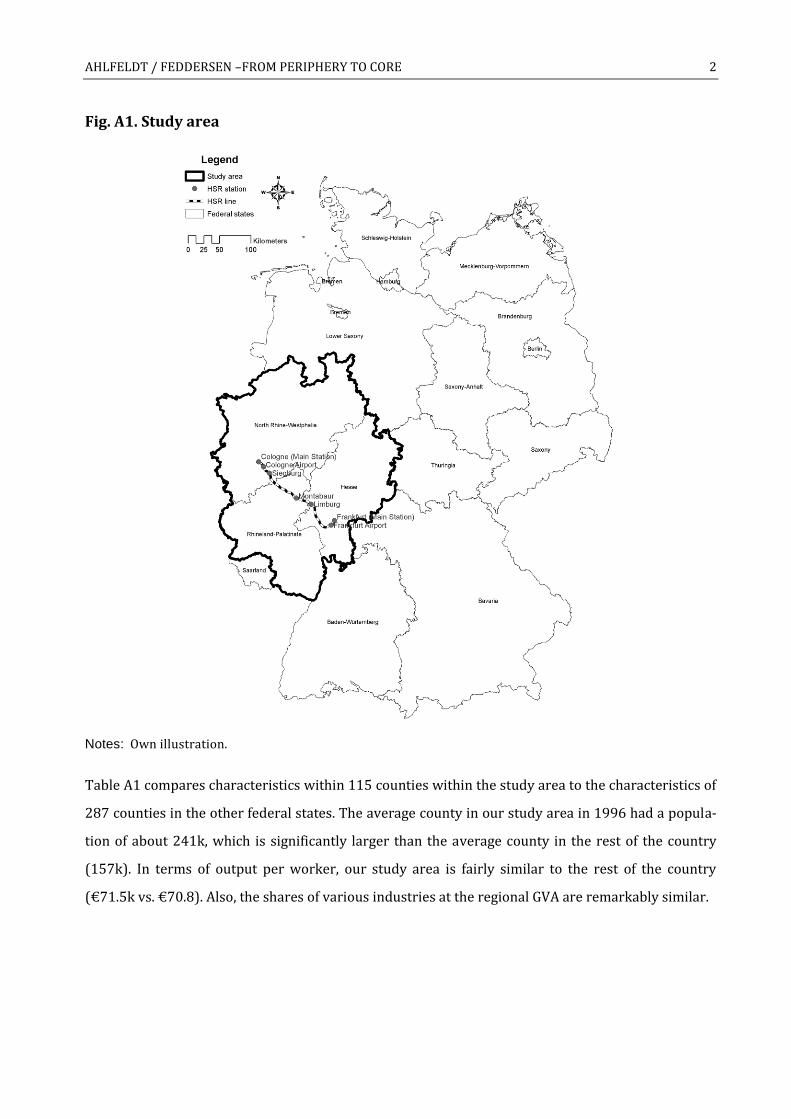
AHLFELDT / FEDDERSEN –FROM PERIPHERY TO CORE 2
Fig. A1. Study area
Notes: Own illustration.
Table A1 compares characteristics within 115 counties within the study area to the characteristics of
287 counties in the other federal states. The average county in our study area in 1996 had a popula-
tion of about 241k, which is significantly larger than the average county in the rest of the country
(157k). In terms of output per worker, our study area is fairly similar to the rest of the country
(€71.5k vs. €70.8). Also, the shares of various industries at the regional GVA are remarkably similar.

AHLFELDT / FEDDERSEN –FROM PERIPHERY TO CORE 3
Tab. A1. County characteristics: Study area vs. rest of Germany
Study area Rest of Germany
1996 Mean S.E. Mean S.E
Population 240,594 14,552 157,219 7,427
GDP (1000 €) 5,787,372 549,684 3,533,259 267,128
GDP/Worker (€) 71,456 740 70,751 546
Share GVA: Construction 2.7% 0.1% 3.7% 0.1%
Share GVA: Mining 13.6% 0.5% 13.2% 0.3%
Share GVA: Other services 33.7% 0.5% 33.1% 0.3%
Share GVA: Retail 9.0% 0.2% 8.8% 0.1%
Share GVA: Manufacturing 16.3% 0.5% 16.9% 0.3%
Share GVA: Financial services 12.9% 0.3% 12.0% 0.1%
Share GVA: Public services 11.8% 0.3% 12.3% 0.2%
Notes: Study area includes 115 counties (NUTS3 regions) in the federal states North Rhine-Westphalia, Hesse, and Rhineland-Palatinate. Rest of Germany includes 287 counties.
3 Program evaluation
This section complements the program evaluation section in the main paper by providing greater
details on the falsification exercises.
A – Falsification I
We begin a with a classic “placebo” study. We use exactly the same empirical design as in the baseline
estimations to estimate the economic impact of an alternative HSR route that was considered during
the planning stages but never built. The track would have had three intermediate stops in each of the
involved federal states and would have passed through the economically and politically relevant cit-
ies of Bonn (the former federal capital located in North Rhine-Westphalia), Koblenz (the largest city
in northern Rhineland-Palatinate) and Wiesbaden (the state capital of Hesse). The exact location of
these intermediate stops is evident from Figure A2 below. A detailed discussion of alternative routes
can be found in Kandler (2002).

AHLFELDT / FEDDERSEN –FROM PERIPHERY TO CORE 4
Fig. A2. Placebo HSR
Notes: Own illustration. The route of the placebo HSR is based on Kandler (2002).
Table A2 summarizes the pre-treatment characteristics of the counties of the placebo intermediate
HSR stops, synthetic control counties constructed for comparison to the placebo treated counties
using the same procedure as in the main paper, and all other non-treated counties in the study area.
The placebo treated counties are economically significantly more potent than the treated counties (in
the main paper), which supports our notion that the HSR treatment at the intermediate stops was
exogenous to their economic strength. Perhaps with the exception of Wiesbaden, the synthetic coun-
ties look very similar to their placebo counterparts.
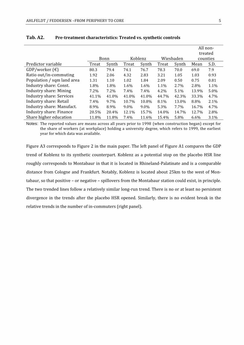
AHLFELDT / FEDDERSEN –FROM PERIPHERY TO CORE 5
Tab. A2. Pre-treatment characteristics: Treated vs. synthetic controls
Bonn Koblenz Wiesbaden
All non-treated
counties Predictor variable Treat Synth Treat Synth Treat Synth Mean S.D. GDP/worker (€) 80.3 79.4 74.1 76.7 78.3 70.0 69.0 7.9
Ratio out/in-commuting 1.92 2.06 4.32 2.83 3.21 1.05 1.03 0.93
Population / sqm land area 1.31 1.10 1.02 1.84 2.09 0.50 0.75 0.81
Industry share: Const. 1.8% 1.8% 1.6% 1.6% 1.1% 2.7% 2.8% 1.1%
Industry share: Mining 7.2% 7.2% 7.4% 7.4% 4.2% 5.1% 13.9% 5.0%
Industry share: Services 41.1% 41.0% 41.0% 41.0% 44.7% 42.3% 33.3% 4.7%
Industry share: Retail 7.4% 9.7% 10.7% 10.8% 8.1% 13.0% 8.8% 2.1%
Industry share: Manufact. 8.9% 8.9% 9.0% 9.0% 5.3% 7.7% 16.7% 4.7%
Industry share: Finance 20.5% 20.4% 12.1% 15.7% 14.0% 14.7% 12.7% 2.8%
Share higher education 11.8% 11.8% 7.4% 11.6% 15.4% 5.8% 6.6% 3.1%
Notes: The reported values are means across all years prior to 1998 (when construction began) except for the share of workers (at workplace) holding a university degree, which refers to 1999, the earliest year for which data was available.
Figure A3 corresponds to Figure 2 in the main paper. The left panel of Figure A1 compares the GDP
trend of Koblenz to its synthetic counterpart. Koblenz as a potential stop on the placebo HSR line
roughly corresponds to Montabaur in that it is located in Rhineland-Palatinate and is a comparable
distance from Cologne and Frankfurt. Notably, Koblenz is located about 25km to the west of Mon-
tabaur, so that positive – or negative – spillovers from the Montabaur station could exist, in principle.
The two trended lines follow a relatively similar long-run trend. There is no or at least no persistent
divergence in the trends after the placebo HSR opened. Similarly, there is no evident break in the
relative trends in the number of in-commuters (right panel).
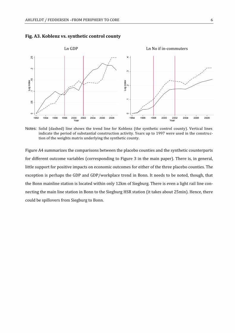
AHLFELDT / FEDDERSEN –FROM PERIPHERY TO CORE 6
Fig. A3. Koblenz vs. synthetic control county
Ln GDP
Ln No if in-commuters
Notes: Solid (dashed) line shows the trend line for Koblenz (the synthetic control county). Vertical lines
indicate the period of substantial construction activity. Years up to 1997 were used in the constru c-tion of the weights matrix underlying the synthetic county.
Figure A4 summarizes the comparisons between the placebo counties and the synthetic counterparts
for different outcome variables (corresponding to Figure 3 in the main paper). There is, in general,
little support for positive impacts on economic outcomes for either of the three placebo counties. The
exception is perhaps the GDP and GDP/workplace trend in Bonn. It needs to be noted, though, that
the Bonn mainline station is located within only 12km of Siegburg. There is even a light rail line con-
necting the main line station in Bonn to the Siegburg HSR station (it takes about 25min). Hence, there
could be spillovers from Siegburg to Bonn.
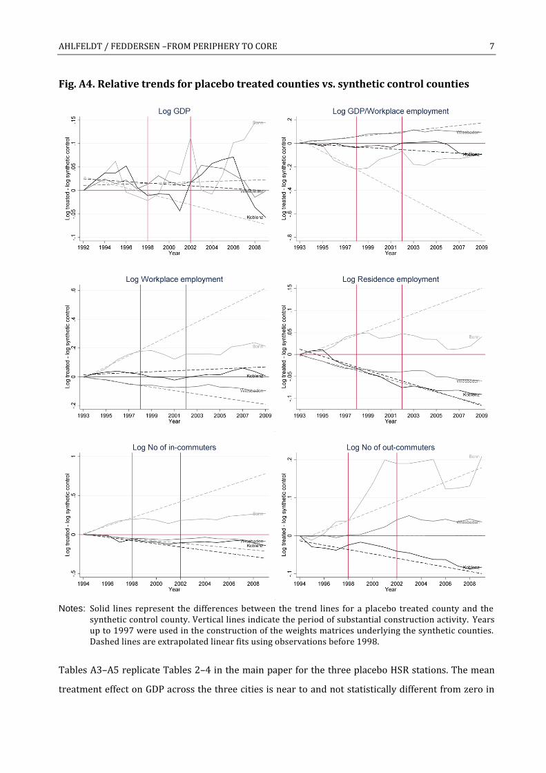
AHLFELDT / FEDDERSEN –FROM PERIPHERY TO CORE 7
Fig. A4. Relative trends for placebo treated counties vs. synthetic control counties
Notes: Solid lines represent the differences between the trend lines for a placebo treated county and the
synthetic control county. Vertical lines indicate the period of substantial construction activity. Years up to 1997 were used in the construction of the weights matrices underlying the synthetic counties. Dashed lines are extrapolated linear fits using observations before 1998.
Tables A3–A5 replicate Tables 2–4 in the main paper for the three placebo HSR stations. The mean
treatment effect on GDP across the three cities is near to and not statistically different from zero in
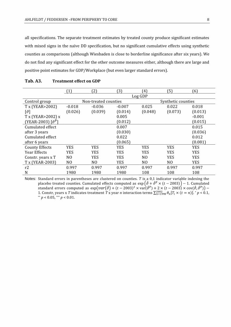
AHLFELDT / FEDDERSEN –FROM PERIPHERY TO CORE 8
all specifications. The separate treatment estimates by treated county produce significant estimates
with mixed signs in the naïve DD specification, but no significant cumulative effects using synthetic
counties as comparisons (although Wiesbaden is close to borderline significance after six years). We
do not find any significant effect for the other outcome measures either, although there are large and
positive point estimates for GDP/Workplace (but even larger standard errors).
Tab. A3. Treatment effect on GDP
(1) (2) (3) (4) (5) (6) Log GDP Control group Non-treated counties Synthetic counties T x (YEAR>2002) [𝜗]
-0.018 (0.026)
-0.036 (0.039)
-0.007 (0.014)
0.025 (0.048)
0.022 (0.073)
0.018 (0.013)
T x (YEAR>2002) x (YEAR-2003) [𝜗P]
0.005 (0.012)
-0.001 (0.015)
Cumulated effect 0.007 0.015 after 3 years (0.030) (0.036) Cumulated effect 0.022 0.012 after 6 years (0.065) (0.081) County Effects YES YES YES YES YES YES Year Effects YES YES YES YES YES YES Constr. years x T NO YES YES NO YES YES T x (YEAR-2003) NO NO YES NO NO YES r2 0.997 0.997 0.997 0.997 0.997 0.997 N 1980 1980 1980 108 108 108
Notes: Standard errors in parentheses are clustered on counties. T is a 0,1 indicator variable indexing the placebo treated counties. Cumulated effects computed as exp (�̂� + �̂�P × (𝑡 − 2003)) − 1. Cumulated standard errors computed as exp(𝑣𝑎𝑟(�̂�) + (𝑡 − 2003)2 × var(�̂�P) + 2 × (𝑡 − 2003) × cov(�̂�, �̂�P)) −1. Constr, years x T indicates treatment T x year n interaction terms ∑ 𝜃𝑛[𝑇𝑖 × (𝑡 = 𝑛)]2002
𝑛=1998 . * p < 0.1, ** p < 0.05, *** p < 0.01.

AHLFELDT / FEDDERSEN –FROM PERIPHERY TO CORE 9
Tab. A4. Treatment effects on GDP by treated county
(1) (2) (3) (4) (5) (6) Log GDP Bonn Koblenz Wiesbaden Control group Non-treat. Synthetic Non-treat. Synthetic Non-treat. Synthetic TREAT x (YEAR>2002) [𝜗]
0.041*** (0.006)
0.039 (0.030)
-0.051*** (0.006)
0.017 (0.073)
-0.043*** (0.006)
-0.003 (0.068)
TREAT x (YEAR>2002) x (YEAR-2003) [𝜗P]
-0.013** (0.004)
-0.022* (0.010)
0.032*** (0.008)
Cumulated effect 0.002 -0.049 0.097 after 3 years (0.041) (0.092) (0.091) Cumulated effect -0.035 -0.110 0.207 after 6 years (0.052) (0.116) (0.115) County Effects YES YES YES YES YES YES Year Effects YES YES YES YES YES YES Constr. years x T NO YES NO YES NO YES T x (YEAR-2003) NO YES NO YES NO YES r2 0.997 1.000 0.997 1.000 0.997 1.000 N 1998 36 1998 36 1998 36
Notes: Standard errors in parentheses are robust in (2), (4) and (6) and clustered on counties in (1), (3), and (5). T is a 0,1 indicator variable indexing the placebo treated counties. Cumulated effects co m-puted as exp (�̂� + �̂�P × (𝑡 − 2003)) − 1. Cumulated standard errors computed as exp(𝑣𝑎𝑟(�̂�) +(𝑡 − 2003)2 × var(�̂�P) + 2 × (𝑡 − 2003) × cov(�̂�, �̂�P)) − 1. Constr, years x T indicates treatment T x year n interaction terms ∑ 𝜃𝑛[𝑇𝑖 × (𝑡 = 𝑛)]2002
𝑛=1998 . * p < 0.1, ** p < 0.05, *** p < 0.01.
Tab. A5. Treatment effect on other economic outcomes
(1) (2) (3) (4) (5) (6) Log
GDP/worker
Log Work-place em-ployment
Log Resi-dence em-ployment
Log popu-lation
Log No of in-commuters
Log No of out-commuters
Control group Synthetic counties T x (YEAR>2002) [𝜗]
0.126 (0.068)
-0.083 (0.070)
-0.008 (0.030)
0.011 (0.014)
-0.037 (0.142)
0.068 (0.049)
T x (YEAR>2002) x (YEAR-2003) [𝜗P]
0.012 (0.022)
-0.009 (0.008)
-0.001 (0.005)
0.000 (0.003)
-0.005 (0.018)
-0.005 (0.007)
Cumulated effect 0.176 -0.103 -0.011 0.012 -0.050 0.056 after 3 years (0.139) (0.096) (0.045) (0.022) (0.213) (0.065) Cumulated effect 0.218 -0.126 -0.014 0.013 -0.064 0.041 after 6 years (0.215) (0.120) (0.060) (0.031) (0.279) (0.082) County Effects YES YES YES YES YES YES Year Effects YES YES YES YES YES YES Constr. years x T YES YES YES YES YES YES T x (YEAR-2003) YES YES YES YES YES YES r2 0.921 0.999 1.000 1.000 0.997 0.998 N 102 102 102 120 96 96
Notes: Standard errors in parentheses are clustered on counties. T is a 0,1 indicator variable indexing the treated counties. Cumulated effects computed as exp (�̂� + �̂�P × (𝑡 − 2003)) − 1. Cumulated standard errors computed as exp(𝑣𝑎𝑟(�̂�) + (𝑡 − 2003)2 × var(�̂�P) + 2 × (𝑡 − 2003) × cov(�̂�, �̂�P)) − 1. Constr, years x T indicates treatment T x year n interaction terms ∑ 𝜃𝑛[𝑇𝑖 × (𝑡 = 𝑛)]2002
𝑛=1998 . * p < 0.1, ** p < 0.05, *** p < 0.01
AHLFELDT / FEDDERSEN –FROM PERIPHERY TO CORE 10
B – Falsification II
Focusing on GDP as an outcome measure we next take the placebo analysis one step further. We run
a series of 1,000 similar placebo models for randomly designed HSR. In each placebo model we first
randomly select one county as one endpoint of the line (the placebo Cologne). Second, we randomly
select another endpoint (the placebo Frankfurt) from all counties within a 140–180km range (in
terms of straight-line distances) of the first endpoint (the distance between Cologne and Frankfurt is
160km). Third, we pick the three counties whose economic center (the largest city) is closest to a
straight line connecting the two endpoints and define them as the treated counties (the placebo in-
termediate stops). Fourth, we create synthetic comparison counties for each of the placebo-treated
counties according to our standard procedure. Fifth, we estimate the naïve DD model (Table 2, col-
umn 3 model, which uses all non-treated control counties and does not control for trends) as well as
our preferred model (Table 2, column 6 model, which uses synthetic control counties and controls
for trends) and save the point estimates and significance levels.
Figure A5 and Table A6 summarize the resulting treatment effects after six years. Of the 1,000 place-
bos 8.4% (24%) deliver significant treatment estimates using our preferred (naïve) DD model. 5.6%
(8.2%) iterations resulted in treatment effects that were significant (at the 10% level) and at least as
large as our benchmark estimates. The means of the point estimates is very close to zero. Notably,
the standard deviation with 8.6% (5.4%) is relatively large compared to our 8.4% (5.7%) treatment
estimate.

AHLFELDT / FEDDERSEN –FROM PERIPHERY TO CORE 11
Fig. A5. Distribution of placebo treatment estimates on GDP
Notes: The black (red) solid line plots the distribution of the placebo treatment estimates after six years
according to our preferred (naïve in Table 2, column 3) DD specification in Table 2, column 6). The vertical black (red) dashed line indicates the benchmark point estimate.
Tab. A6. Distribution of placebo treatment effects on GDP
Control Group
All non-treated counties Synthetic counties
Coeff. p-value p-value<0.1 Coeff. p-value p-value<0.1
Obs 1000 1000 1000 1000 1000 1000
Mean 0.000 0.371 0.240 -0.007 0.501 0.084
Std. Dev. 0.047 0.306 0.428 0.096 0.277 0.278
Min -0.117 0.000 0.000 -0.262 0.001 0.000
Max 0.150 0.996 1.000 0.512 0.999 1.000
Notes: Placebo treatment estimates after six years based on Table 2, column (3) and (6) specifications.
4 Agglomeration effects
This section complements section 4 of the main paper by providing additional results not reported in
the main paper for brevity.

AHLFELDT / FEDDERSEN –FROM PERIPHERY TO CORE 12
A – Alternative spatial decay in market potential
The exponential functional form of the spatial decay in spillovers, while popular in the theoretical
and empirical literature (e.g., Ahlfeldt, Redding, Sturm, & Wolf, 2015; Fujita & Ogawa, 1982; Lucas &
Rossi-Hansberg, 2002), is ad-hoc and other functional forms are theoretically imaginable. To evalu-
ate the sensitivity of the results to the chosen functional form of the spatial decay in the market po-
tential we estimate an alternative to specification (4-3).
ln(𝑄𝑖,𝑡=2002) − ln(𝑄𝑖,𝑡=1998) = 𝛿0 + ∑ δ1,m(𝐵𝑚,𝑖,2002 − 𝐵𝑚,𝑖,1998)𝑚
+ ∆휀𝑖
, where 𝐵𝑚,𝑖,t indicates the total GDP in all counties within a certain effective distance ring m in year
t={1998,2002}. We group counties with mutually exclusive 20-minute travel time bins (e.g., 0–20min,
20–40min, …, 140–160min). For each travel time bin a separate market potential elasticity δ1,m is
estimated, thus allowing for a more flexible pattern in the spatial decay. In Figure A6 we compare the
predicted effects of the change in market potential on GDP in this alternative model to our baseline
model. We find an approximately linear relationship, suggesting that our results are not driven by an
inappropriate functional form of the spatial decay.
Fig. A6. Parametric vs. semi-parametric fitted values
Notes: Dashed line is the lowess fitted line (bandwidth of 0.8). Solid line is the 45 degree line.
AHLFELDT / FEDDERSEN –FROM PERIPHERY TO CORE 13
B – Alternative travel time matrices
To approximate the effective change in accessibility induced by HSR in our study area we have made
a number of assumptions regarding the effective travel costs on different parts of the transport net-
work and the way travelers are able to combine these segments. In this section, we experiment with
different travel choice decision rules to evaluate the degree to which our results depend on the as-
sumptions made. In our benchmark model, which for the purpose of comparison we replicate in Ta-
ble A7, column (1), we allow for a great degree of choice in finding the optimal route through the
combined road and rail network. Travelers are allowed to switch mode at HSR stations, i.e., they can
use their cars to travel to an HSR station, then switch to the HSR train, and then switch back to the
road networks (e.g., using a taxi or a rental car).
In column (2) we replicate the model with a more restrictive transport decision model. Travelers are
assumed to choose the least-cost mode for a given origin-destination combination in any given peri-
od, but they are not allowed to switch mode during a journey. An HSR trip can only be combined with
a conventional rail trip, but not the road network. As road trips are typically faster than conventional
rail trips (because of higher speeds on highways), forcing HSR passengers onto the conventional rail
network for the remaining parts of their journey results in a lower impact of HSR on travel times
within our study area. Based on this more restrictive transport choice and the parameter estimates
in column (2) the implied maximum impact on market potential (for Westerwaldkreis, the home
county of the Montabaur stop) is 0.27 log points, which is less than the 0.34 effect in model (1). Not
surprisingly, given the smaller variation in change in market potential we find a larger market poten-
tial elasticity than in the baseline model. For Montabaur, the estimated market potential elasticity
and the change in market potential implies a predicted effect on GDP of 6%, which is virtually identi-
cal to the benchmark model.
In column (3) we ignore the road network altogether and force travelers on the rail network for all
trips in any period. As this change slows travelers down on virtually all trips that do not benefit from
HSR, the impact of HSR on travel times becomes significantly larger. The increase in market potential
for Montabaur amounts to 0.65 log points, which is almost twice as much as in the baseline model.
While the market potential elasticity is lower than in the baseline model as expected, the estimated
parameters in column (3) along with the changes in bilateral travel cost imply a predicted GDP im-
pact of 8%, which is only slightly higher than in the baseline model. In column (4) we extend model
(3) by a market potential measure that only incorporates the road network (we restrict the decay

AHLFELDT / FEDDERSEN –FROM PERIPHERY TO CORE 14
parameter to be the same as in the change in rail market potential) to disentangle the accessibility
benefits induced by HSR from trends correlated with road accessibility. The results remain almost
unchanged.
Finally, we use a mix of the transport matrices used in (2) and (3) in model (5). Making the heroic
assumption that 50% of travelers use either the road or the rail network in any period and on every
route we compute the average of the road and rail travel times. While the maximum accessibility
effect of 0.32 log points is almost identical to the benchmark estimate the market potential elasticity
is notably larger, implying a larger (maximum) predicted effect on GDP.
A notable finding that emerges from the comparison of the estimates presented in Table A7 is that
the decay parameter is reassuringly stable. The comparison across these models further reassures
our decision to use model (1) as a benchmark model because it not only allows for relative flexible
transport choices, but the model also delivers a combination of relatively high explanatory power
and a conservative estimate of the market potential elasticity.

AHLFELDT / FEDDERSEN –FROM PERIPHERY TO CORE 15
Tab. A7. Agglomeration effects by transport cost matrix
Notes: Estimation method is nonlinear least squares in all models. Robust standard errors (in parentheses) of the market potential coefficient 𝛿1 are heteroscedasticity robust and computed in separate OLS regressions holding the decay parameters (𝛿2) constant at the levels estimated in the NLS models re-ported in the table. The market potential of region i is the transport cost weighted sum of output in all regions j. The change in market potential is driven by changes in travel cost between regions ex-clusively. Regional output is held constant at 1998 level. * p < 0.1,
** p < 0.05,
*** p < 0.01.
B – Alternative 2SLS models
At the heart of our identification strategy we argue that the timing of the construction and opening of
the HSR is exogenous to the economic trends during the analyzed adjustment period as planning had
been initiated several decades prior to then. We also argue that the timing and the routing is plausi-
bly exogenous for the intermediate stops as the purpose of the line was to connect the endpoints and
the intermediate stops resulted from political bargaining rather than economic reasoning. As such,
the arguably most credible identification stems from counties that lie in-between Cologne and Frank-
furt and benefit from improved access through the intermediate stops at Limburg, Montabaur, and
Siegburg.
In Table A8 we therefore restrict the information used to identify the market potential effect to this
most plausibly exogenous fraction using a 2SLS estimation strategy. We consider three different sets
of instrumental variables: the log of the straight-line distance to Montabaur station, which is the loca-
tion that experienced the largest accessibility gain (see Figure 1 in the main paper), three indicator
dummy variables for the counties of the three intermediate stops (used in column 5 of Table 6 in the
main paper), and the same plus six additional indicator variables for the adjacent counties. We use
for each of these instrumental variable strategies, excluding (1–3) and including (4–6), the covariates
used in Table 6 in the main text. We find that any of the 2SLS models produces results that are simi-
(1) (2) (3) (4) (5) Δln GDP 1998-2002 Δln Market potential (𝛿1)
0.185*** (0.051)
0.225** (0.069)
0.126*** (0.031)
0.129*** (0.030)
0.251*** (0.063)
Decay (𝛿2) 0.022* 0.023* 0.020** 0.021*** 0.021** (0.011) (0.013) (0.008) (0.007) (0.008) Ln market potential 1998 (automobile)
-0.016 (0.010)
Combination of modes allowed
Auto, rail, rail & HSR, auto & HSR
Auto, rail, rail & HSR
Rail, rail & HSR
Rail, rail & HSR
50% rail or rail & HSR, 50% auto
Spillover elasticity (𝛽) 0.028 0.034 0.019 0.019 0.038 N 115 115 115 115 115 r2 0.054 0.037 0.059 0.085 0.059
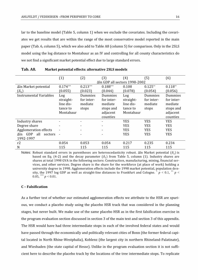
AHLFELDT / FEDDERSEN –FROM PERIPHERY TO CORE 16
lar to the baseline model (Table 5, column 1) when we exclude the covariates. Including the covari-
ates we get results that are within the range of the most conservative model reported in the main
paper (Tab. 6, column 5), which we also add to Table A8 (column 5) for comparison. Only in the 2SLS
model using the log distance to Montabaur as an IV and controlling for all county characteristics do
we not find a significant market potential effect due to large standard errors.
Tab. A8. Market potential effects: alternative 2SLS models
(1) (2) (3) (4) (5) (6) Δln GDP all sectors 1998-2002 Δln Market potential (𝛿1)
0.174*** (0.055)
0.213*** (0.023)
0.188*** (0.044)
0.108 (0.078)
0.125** (0.054)
0.118** (0.056)
Instrumental Variables Log straight-line dis-tance to Montabaur
Dummies for inter-mediate stops
Dummies for inter-mediate stops and adjacent counties
Log straight-line dis-tance to Montabaur
Dummies for inter-mediate stops
Dummies for inter-mediate stops and adjacent counties
Industry shares - - - YES YES YES Degree share - - - YES YES YES Agglomeration effects - - - YES YES YES Δln GDP all sectors 1992-1997
- - - YES YES YES
r2 0.054 0.053 0.054 0.217 0.235 0.234 N 115 115 115 115 115 115
Notes: Robust standard errors in parentheses are heteroscedasticity robust. Δln Market potential (𝛿1) is based on Eq. (4-2) and the decay parameter (𝛿1) from Table 5, column (1). Industry shares are shares at total 1998 GVA in the following sectors: Construction, manufacturing, mining, financial ser-vices, and other services. Degree share is the share for the workforce (at place of work) holding a university degree in 1998. Agglomeration effects include the 1998 market potential, population de n-sity, the 1997 log GDP as well as straight-line distances to Frankfurt and Cologne. *
p < 0.1, **
p <
0.05, ***
p < 0.01.
C – Falsification
As a further test of whether our estimated agglomeration effects we attribute to the HSR are spuri-
ous, we conduct a placebo study using the placebo HSR track that was considered in the planning
stages, but never built. We make use of the same placebo HSR as in the first falsification exercise in
the program evaluation section discussed in section 3 of the main text and section 3 of this appendix.
The HSR would have had three intermediate stops in each of the involved federal states and would
have passed through the economically and politically relevant cities of Bonn (the former federal capi-
tal located in North Rhine-Westphalia), Koblenz (the largest city in northern Rhineland-Palatinate),
and Wiesbaden (the state capital of Hesse). Unlike in the program evaluation section it is not suffi-
cient here to describe the placebo track by the locations of the tree intermediate stops. To replicate

AHLFELDT / FEDDERSEN –FROM PERIPHERY TO CORE 17
the analysis of agglomeration effects we require a full matrix of the bilateral travel times that incor-
porates the alternative HSR routing.
As the exact routing of this line was never finalized we approximate a plausible route based on the
information released during the planning stages and the decision rules employed in the design of the
actual line. The alternative line was intended to largely follow the river Rhine, but it was clear that
for a section south of Koblenz the terrain was too mountainous to allow for very high speeds
(Kandler, 2002). We therefore construct the placebo track parallel to the Rhine north of Koblenz and
parallel to the highways A61, A66, and A3 south of Koblenz. As discussed in the main text, a similar
approach was followed with the actual HSR, which in large part runs parallel to the A3. The routing of
the placebo HSR is illustrated in Fig A2. In constructing bilateral travel times we employ exactly the
same travel cost parameters and decisions rules as in the baseline transport decision model dis-
cussed in section 4-B in the main text..
In Figure A7 we compare the resulting distribution of bilateral travel times (solid red line) to the
distribution of travel times on the road network (pre-HSR, black solid line) and the distribution of
combined network times including the actual HSR (red dashed line). Not surprisingly, given the fact
that the placebo HSR connects the same endpoints at the same speed (albeit along a slightly longer
route), the resulting travel time distribution resembles the one of the actual HSR scenario quite
closely.
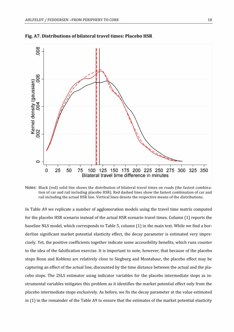
AHLFELDT / FEDDERSEN –FROM PERIPHERY TO CORE 18
Fig. A7. Distributions of bilateral travel times: Placebo HSR
Notes: Black (red) solid line shows the distribution of bilateral travel times on roads (the fastest combina-tion of car and rail including placebo HSR). Red dashed lines show the fastest combination of car and rail including the actual HSR line. Vertical lines denote the respective means of the distributions.
In Table A9 we replicate a number of agglomeration models using the travel time matrix computed
for the placebo HSR scenario instead of the actual HSR scenario travel times. Column (1) reports the
baseline NLS model, which corresponds to Table 5, column (1) in the main text. While we find a bor-
derline significant market potential elasticity effect, the decay parameter is estimated very impre-
cisely. Yet, the positive coefficients together indicate some accessibility benefits, which runs counter
to the idea of the falsification exercise. It is important to note, however, that because of the placebo
stops Bonn and Koblenz are relatively close to Siegburg and Montabaur, the placebo effect may be
capturing an effect of the actual line, discounted by the time distance between the actual and the pla-
cebo stops. The 2SLS estimator using indicator variables for the placebo intermediate stops as in-
strumental variables mitigates this problem as it identifies the market potential effect only from the
placebo intermediate stops exclusively. As before, we fix the decay parameter at the value estimated
in (1) in the remainder of the Table A9 to ensure that the estimates of the market potential elasticity
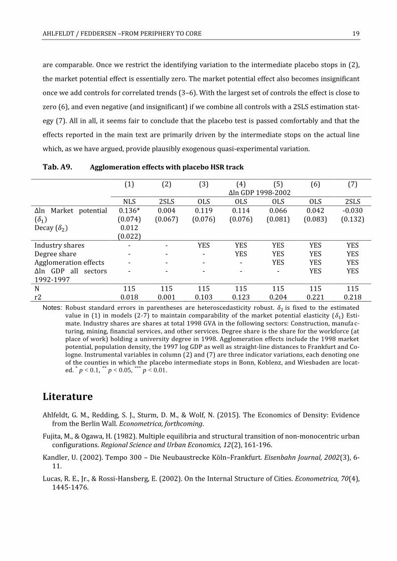
AHLFELDT / FEDDERSEN –FROM PERIPHERY TO CORE 19
are comparable. Once we restrict the identifying variation to the intermediate placebo stops in (2),
the market potential effect is essentially zero. The market potential effect also becomes insignificant
once we add controls for correlated trends (3–6). With the largest set of controls the effect is close to
zero (6), and even negative (and insignificant) if we combine all controls with a 2SLS estimation stat-
egy (7). All in all, it seems fair to conclude that the placebo test is passed comfortably and that the
effects reported in the main text are primarily driven by the intermediate stops on the actual line
which, as we have argued, provide plausibly exogenous quasi-experimental variation.
Tab. A9. Agglomeration effects with placebo HSR track
(1) (2) (3) (4) (5) (6) (7) Δln GDP 1998-2002 NLS 2SLS OLS OLS OLS OLS 2SLS Δln Market potential (𝛿1)
0.136* (0.074)
0.004 (0.067)
0.119 (0.076)
0.114 (0.076)
0.066 (0.081)
0.042 (0.083)
-0.030 (0.132)
Decay (𝛿2) 0.012 (0.022) Industry shares - - YES YES YES YES YES Degree share - - - YES YES YES YES Agglomeration effects - - - - YES YES YES Δln GDP all sectors 1992-1997
- - - - - YES YES
N 115 115 115 115 115 115 115 r2 0.018 0.001 0.103 0.123 0.204 0.221 0.218
Notes: Robust standard errors in parentheses are heteroscedasticity robust. 𝛿2 is fixed to the estimated value in (1) in models (2-7) to maintain comparability of the market potential elasticity (𝛿1) Esti-mate. Industry shares are shares at total 1998 GVA in the following sectors: Construction, manufa c-turing, mining, financial services, and other services. Degree share is the share for the workforce (at place of work) holding a university degree in 1998. Agglomeration effects include the 1998 market potential, population density, the 1997 log GDP as well as straight-line distances to Frankfurt and Co-logne. Instrumental variables in column (2) and (7) are three indicator variations, each denoting one of the counties in which the placebo intermediate stops in Bonn, Koblenz, and Wiesbaden are locat-ed. * p < 0.1,
** p < 0.05,
*** p < 0.01.
Literature
Ahlfeldt, G. M., Redding, S. J., Sturm, D. M., & Wolf, N. (2015). The Economics of Density: Evidence from the Berlin Wall. Econometrica, forthcoming.
Fujita, M., & Ogawa, H. (1982). Multiple equilibria and structural transition of non-monocentric urban configurations. Regional Science and Urban Economics, 12(2), 161-196.
Kandler, U. (2002). Tempo 300 – Die Neubaustrecke Köln–Frankfurt. Eisenbahn Journal, 2002(3), 6-11.
Lucas, R. E., Jr., & Rossi-Hansberg, E. (2002). On the Internal Structure of Cities. Econometrica, 70(4), 1445-1476.

AHLFELDT / FEDDERSEN –FROM PERIPHERY TO CORE 20

Spatial Economics Research Centre (SERC)London School of EconomicsHoughton StreetLondon WC2A 2AE
Tel: 020 7852 3565Fax: 020 7955 6848Web: www.spatialeconomics.ac.uk
SERC is an independent research centre funded by the Economic and Social Research Council (ESRC), Department for Business Innovation and Skills (BIS) and the Welsh Government.