Chaos in the Core-Periphery Model1

by Martin Currie

The University of Manchester and

Ingrid Kubin University of Economics and Business Administration, Vienna

February 2003

1. Introduction

The two-region core-periphery model, developed by Paul Krugman (1991a, 1999b), has become

the basis of a paradigm – the New Economic Geography – that seeks to integrate urban

economics, regional science and international trade in a single theoretical framework and, more

generally, to rectify the omission of space from mainstream economics. The Spatial Economy:

Cities, Regions and International Trade, by Fujita, Krugman and Venables – henceforth FKV –

encompasses various developments of that model. In their Introduction, FKV pose the two basic

questions that recur throughout their work and they anticipate their methodology for addressing

them. They address the first question “when is a spatial concentration of economic activity

sustainable?” by positing that all manufacturing is concentrated in one region and asking whether

a worker who moved to the other region would improve his real wage. If the answer is “yes”, a

core-periphery equilibrium would not be sustainable. They address the second question “when is

a symmetric equilibrium, without spatial concentration, unstable?” by asking whether, starting

from a symmetric equilibrium, a movement of a small number of workers from one region to the

other raises or lowers the relative wage in the destination region. If it raises it, the symmetric

equilibrium is unstable against small perturbations; if it lowers it, the symmetric equilibrium is

stable. The basic model is used to derive propositions about the impacts on the geographical

location of industry of changes in transport costs, in expenditure shares devoted to manufactured

goods and in the consumers’ preference for variety.

It is important to scrutinise carefully the robustness of any model that is the basis for a

new paradigm, particularly one which is used to tell ‘stories of breathtaking scope’ (FKV, p.

1 We are grateful for extremely helpful comments on an earlier version from Pasquale Commendatore, Paul Madden, Pierre Picard and Trevor Young.

2

277). The purpose of this paper is to examine whether the propositions derived from the standard

core-periphery model are robust with respect to the temporal framework. Our only substantive

modification of the standard continuous-time core-periphery model is to re-formulate it in

discrete time. The implications of doing so are profound. The possible long-term behaviours are

no longer confined to a symmetric equilibrium or to the core-periphery equilibria but may

involve the periodic or chaotic coexistence of two active manufacturing sectors. Moreover, the

methodology of positing an equilibrium and identifying the impact of the movement of a small

number of workers on real wages is not reliable in a discrete-time framework. For example, it

may be that the system is attracted to a core-periphery equilibrium, notwithstanding that a

worker who moved from the core to the periphery would improve his real wage. Furthermore,

given that asymmetric coexistence is possible, the standard propositions about the impact of

changes in parameters need to be re-assessed.

We explain the model in Section 2. It involves the familiar assumption of two regions,

each with agricultural and manufacturing sectors.2 Each region has the same number of farmers,

farmers being immobile. The manufacturing sectors involve Dixit-Stiglitz monopolistic

competition, with instantaneous entry and exit. Workers migrate between the manufacturing

sectors in response to economic incentives. In Section 3, we characterise a short-run general

equilibrium contingent on the regional allocation of the manufacturing workforce. In particular,

we focus on the determination of the ratio of the real manufacturing wage rates, since it is the

latter that drives worker migration in our model. We also explain why we do not invoke all the

standard core-periphery normalisations. In Section 4, we examine the stationary equilibria for the

model and we review, from the standard continuous-time perspective, the stability properties of

these equilibria. In Section 5, we explore the remarkably complex dynamical behaviour of the

discrete-time core-periphery model. We allude briefly to possible amendments to the model in

Section 6 and offer some concluding comments in Section 7.

2. Model

Consumers in both regions have Cobb-Douglas preferences over a homogeneous agricultural

good and a quantity index that is a CES function of the varieties of manufactured goods. The

exponents of the agricultural good and of the manufacturing composite in the common utility

function – and therefore the invariant shares of income devoted to the agricultural good and to

2 We take as our point of reference the model presented in Chapter 5 of FKV’s work. A lucid exposition is also provided in Neary (2001).

3

manufactures – are ( )1 µ− and µ, respectively. The constant elasticity of substitution between

the manufactured varieties is denoted by 1σ > ; the lower σ, the greater the consumers’ taste for

variety.

Farm labour is the sole scarce agricultural input. Farmers are immobile: the total number

of farmers is F, with half of the farmers in each region. Each farmer provides one unit of labour;

and one unit of farm labour yields one unit of the agricultural product. Transportation of the

agricultural product between regions is costless. Consequently, with instantaneous establishment

of equilibrium in the agricultural market, the agricultural price is the same in both regions.

Furthermore, given the constant returns to scale in agriculture, the nominal wage rate of farmers

is equal to the agricultural price. As is standard, we take the nominal agricultural wage rate as the

numeraire, so that the price of the agricultural product is also 1.

In contrast to farmers, manufacturing workers are mobile between regions at the

transitions between time periods. The total number of workers, denoted by L, is invariant over

time. Region 1’s share of the manufacturing workforce at the beginning of period t is denoted by

tλ , where 0 1tλ≤ ≤ . Manufacturing uses solely the labour of workers but, in contrast to

agriculture, involves increasing returns. The production technology is the same for each variety:

each manufacturer requires a fixed labour input of α to operate and has a constant marginal

labour requirement β. The manufacturing sectors involve Dixit-Stiglitz monopolistic

competition. Given the consumers’ preference for variety and given the increasing returns, a

particular variety is never produced by more than one firm; i.e., an entrant would always produce

a different variety from those produced by active firms. Furthermore, since manufacturers in the

same region face the same wage rate, each sets the same mill price ,r tp and supplies the same

quantity ,r tq using the same labour input ,r tl , where , ,r t r tl qα β= + . Each manufacturer uses the

price-setting rule:

(1) , ,1r t r tp wβσσ

=−

where ,r tw is the nominal wage rate in region r in period t and where ( )1βσ σ − is a time-

invariant price-wage mark-up. This pricing rule is optimal for a firm given that it believes that

others will not react to its own price decision and given that it ignores the indirect impact of a

change in its own price on demand via its effect on the manufacturing price index. These Dixit-

Stiglitz assumptions are more plausible the larger the number of manufacturers.

Transport costs for manufactures take an iceberg form: if 1 unit is shipped between

regions, 1 T arrives where 1T > . Consequently the effective price paid by consumers in the

4

other region for a variety produced in region r is ,r tp T . The manufacturing price indices facing

consumers in the regions are:

(2) 1 1

1 1 1 1 1 11 11, 1, 1, 2, 2, 2, 1, 1, 2, 2,t t t t t t t t t tG n p n p T G n p T n pσ σ σ σ σ σσ σ− − − − − −− − = + = +

where ,r tn is the number of varieties produced in region r. The nominal regional incomes are:

(3) ( )1, 1, 2, 2, 12 2t t t t t tF FY w L Y w Lλ λ= + = + −

The product demands are then:

(4) 1 1 1 1 1 11, 1 1, 2 2, 1, 2, 1 1, 2 2, 2,t t t t t t t td Y G Y G T p d Y G T Y G pσ σ σ σ σ σ σ σµ µ− − − − − − − − = + = +

where σ− is the price elasticity as perceived by each manufacturer and where ,r td is the demand

for a variety produced in region r. Using (1), (2), (3) and (4), the product demands depend on the

numbers of varieties and indirectly on the workforce allocation and on the nominal wage rates.

Given that the agricultural price is 1, the real wage rates are:

(5) 1, 1, 1, 2, 2, 2,t t t t t tw G w Gµ µω ω− −= =

Workers move between regions at the transitions between time periods in response to economic

incentives. The migration process is:

(6) ( )1,1

2,

ln 1tt t t t

t

Lω

λ λ γ λ λω+

= + −

subject to 10 1tλ +≤ ≤

where 0γ > is the migration speed. This process, where migration depends on the ratio of the

real wage rates, differs from the FKV process, ( ) ( )1 2 1λ γ ω ω λ λ= − − , where migration depends

on the difference in real wage rates. Note that, both for (6) and for the FKV process, workers do

not move to a region with no manufacturing sector in the previous period, i.e., 0tλ = implies

1 0tλ + = . In terms of the number of net migrants, process (6) is equivalent to

(7) 1,1, 1 1, 1, 2,

2,

ln tt t t t

t

L L L Lω

γω+

− =

subject to 1, 10 tL L+≤ ≤

where 1,t tL Lλ= and ( )2, 1t tL Lλ= − . Process (7) is a discrete-time counterpart of the migration

process assumed by Puga (1998).3

3 Puga’s rationale for such a process is along the following lines. Opportunities to migrate to region r arrive at a Poisson rate ,r tLρ . Given the opportunity to migrate from region s to region r, a worker wishes to do so if

, ,r t s t cω ω > , where c is a migration cost randomly drawn from a distribution with density function ( ) 1dF c cδ= in

the interval 1,eδ and zero elsewhere. The probability that an individual worker in region s has an incentive to

5

3. Short-run General Equilibrium

At the beginning of period t, there is a given regional allocation of the workforce, tλ . In this

Section, we characterise a short-run general equilibrium contingent on that allocation. Following

FKV, we assume instantaneous entry and exit of manufacturers, ensuring zero pure profits in

each period. This assumption has the powerful implication that the number of varieties /

manufacturers in a region is proportional to the regional workforce. Zero pure profit requires that

for an active manufacturer in region r in period t:

(8) ( ), , , , , , , , 0r t r t r t r t r t r t r t r tp q w l p q w qα β− = − + =

From (1) and (8):

(9) ( ),

1r tq q

α σβ−

= = ,r tl q lα β ασ= + = =

That is, instantaneous entry and exit implies that the scale of each firm – and the output per

variety – is invariant over time. Given 0 1tλ< < , short-run general equilibrium requires that the

derived demand for workers equal the supply of workers simultaneously in both regions:

(10) ( ) ( ) ( )1, 1, 2, 2, 1t t t t t tn d L n d Lα β λ α β λ+ = + = −

Since product demands are satisfied:

(11) 1, 2,t td d q= =

i.e., the demand per variety is the same in both regions. With full employment, it follows from

(9) that the short-run equilibrium numbers of manufacturers / varieties are:

(12) ( ) ( )1, 2,

11tt

t t t t

LL L Ln nl l

λλ λ λασ ασ

−= = = = −

This confirms that the total number of varieties, L ασ , is invariant over time, and that in period

t the number of varieties in a region is proportional to the regional workforce. From Walras’

Law, labour market equilibrium in one region implies labour market equilibrium in the other

region. Given zero profits in both agriculture and manufacturing, the ratio of the total nominal

incomes of workers to the total nominal incomes of farmers corresponds to the ratio of the

expenditure shares:

(13) ( )1, 2, 1

1t t t tw L w L

Fλ λ µ

µ+ −

=−

move is ( ) ( ), ,1 ln r t s tδ ω ω ; and the number with such an incentive is ( ) ( ), , ,1 ln r t s t s tLδ ω ω . The migration speed in

(6) and (7) is then γ ρ δ≡ .

6

Consequently:

(14) ( )1, 2, 1t t t tw wλ λ+ − = Ω

where

(15) ( )1FL

µµ

Ω =−

Given the worker migration process, we are ultimately interested in the ratio of the real

wage rates. From (1), (4) and (11), the relevant nominal ratios satisfy:

(16) ( ) ( )( ) ( )

1 11, 2, 1, 2,1,

112, 1, 2, 1, 2,

t t t tt

t t t t t

Y Y G G Tww Y Y T G G

σσ σ

σσ

− −

−−

+ = +

From (1), (2) and (12):

(17) ( ) ( )( ) ( )

11 11, 2,1,

1 12, 1, 2,

1

1t t t tt

t t t t t

w w TGG w w T

σσ σ

σ σ

λ λ

λ λ

−− −

− −

+ − = + −

From (3) and (13):

(18) ( ) ( ) ( )( )( ) ( ) ( )( )

1, 2,1,

2, 1, 2,

1 1 11 1 1

t t t tt

t t t t t

w wYY w w

µ λ µ λµ λ µ λ

+ + − −=

− + + −

Substituting (17) and (18) into (16) gives the nominal wage rate ratio, 1, 2,t tw w , as an implicit

function of the workforce allocation, tλ :

(19)

( )

( )

( )

( )

1

1, 1, 1

2, 2, 11

1, 1, 1

2, 2,1,

2, 1,

2,

1,

2,

1 11 1

1 1 11 1

1 11

1 11

t tt t

t t t t

tt tt

t t t tt

t tt

t t

tt

t t

w wT

w wT

w wTw ww

w wwww

σ

σ

σσ

σσ

λ λµ µλ λ

λ λµ µλ λ

λµ µλ

λµ µλ

−

−

−−

−

+ + − + − − +

+ + + + − − = + + − −

+ + + −

1

1, 1

2,11

1, 1

2,

1

11

tt

t t

tt

t t

wT

wT

wT

w

σ

σ

σσ

σ

λλ

λλ

−

−

−−

−

+ − +

+ −

Having determined 1, 2,t tw w , 1, 2,t tG G is determined from (17). The ratio of the real wages is

then given by:

(20) 1, 1, 2,

2, 2, 1,

t t t

t t t

w Gw G

µωω

=

The complexity of the core-periphery model is such that (19) cannot be solved analytically.

However, for given parameter values, numerical solutions can be obtained by a computer (as the

7

market mechanism is assumed able to do). Figure 1 shows, for 5σ = and 0.4µ = , the

relationship between 1, 2,t tω ω and tλ for different transport costs: (a) 1.5T = ; (b) 1.63T = ; (c)

1.75T = ; (d) 1.81T = ; and (e) 2T = . We refer frequently to these diagrams.

The dynamical behaviour of the system is driven by the dependence of the short-run

general equilibrium real wage ratio on the workforce allocation and by the impact of the real

wage ratio on worker migration. Note well that the technological parameters, α and β , and the

factor endowments, F and L, do not affect the ratio of the real wage rates. Consequently the

nature of the system’s dynamical behaviour does not depend on α , β or F, and it depends on L

solely via the worker migration process. The dynamical behaviour depends also on the utility

parameters σ and µ ; on the transport cost parameter T; and on the worker migration speed γ .

As a postscript to this Section, we note why we did not impose certain normalisations that

are invoked as a matter of course in presentations of the core-periphery model, namely, that units

of measurement are chosen so that ( )1β σ σ= − and so that α µ σ= . It is not self-evident to

us what it means to employ equilibrium solutions based on such normalisations to identify the

impact of a change in, say, σ . Presumably one is not meant to suppose that either some unit of

measurement or β is being altered so that ( )1β σ σ= − is maintained. Our main reason for

positing that worker migration depends on the ratio of the real wage rates is that this ratio is, and

is shown to be, independent of α and β . In contrast, changes in α or in β affect the levels of

1,tG and 2,tG and, thereby, affect the levels of the nominal and real wage rates and, thereby,

affect the difference in real wage rates. Consequently, with a discrete-time counterpart of the

FKV assumption that migration depends on the difference in real wage rates, the system’s

dynamical behaviour would depend on α and β . FKV further assume that units of

measurement are chosen so that L µ= and 1F µ= − (which from (15) implies 1Ω = ). Whereas

changes in F and L do not alter the ratio of real wage rates, they do alter the difference in real

wage rates.

4. Stationarity

In this Section, we examine thorough-going stationary states for the standard core-periphery

model. We can immediately identify two types of long-run equilibria. The first is the symmetric

stationary equilibrium with 1 2λ λ= = . The corresponding stationary values are:

ratio

ofre

alw

ages

1

1

0 1

region 1's share of workforce

1

1

1

(e)

(d)

(c)

(b)

(a)

λ

λ

1 2λ =

Figure 1

8

(21) w = Ω1

p βσσ

= Ω− 2

Lnασ

=1 1

11 11G n T pσσ σ−− − = + wG µω −=

Not only are the conditions for short-run general equilibrium met; in addition, the equality of real

wage rates means that there is no incentive for workers to move between the regions. The second

type is a core-periphery equilibrium in which all manufacturing activity is agglomerated in one

(either) region. In the core, the stationary values are:

(22) Cw = Ω1Cp βσ

σ= Ω

− CLn

ασ=

11

C C CG n pσ−= C C Cw G µω −=

In the periphery, they are:

(23) 1

1 11 12 2Pw T T

σσ σµ µ− −− + = Ω + 0Pn =

11

P C CG n p Tσ−= P P Pw G µω −=

where Pw and Pω should be interpreted as virtual wages, since no actual labour transactions take

place, but where PG is an actual price index facing farmers as consumers in the periphery. This

is a stationary equilibrium, since workers do not migrate to a region with no manufacturing

sector.

Particular attention has been paid in the New Economic Geography to the significance of

transport costs for the number and nature of the long-run equilibria. The so-called ‘tomahawk

bifurcation’ in Figure 2 is widely used to illustrate this. Solid lines designate locally stable long-

run equilibria and dotted lines designate unstable long-run equilibria. What is deemed to be

locally stable or unstable derives from a continuous-time analysis of the process of worker

migration. In order to provide a basis with which to compare our discrete-time analysis, we now

explain the continuous-time derivation of the tomahawk bifurcation; in doing so, we interpret the

short-run general equilibrium characterised in Section 3 as an ‘instantaneous equilibrium’. For

such a continuous-time analysis, as long as workers move continuously to the region with the

higher real wage rate, the precise migration process – and the speed of migration – do not matter:

the direction of movement can be inferred from Figure 1.4

There are two critical levels of the transport cost parameter in Figure 2: BT is called the

break point and ST is called the sustain point. The defining characteristic of BT is that the rate of

change of the ratio of real wage rates (or of the difference in real wage rates) with respect to λ is

0 at the fixed point 1 2λ = . It can be shown that:

4 Both FKV and Puga (1998) emphasise that the precise form of the migration process does not matter.

0

1

1 T

λ

BT ST

Figure 2

1 2λ =

9

(24) ( )

( )

1111 1

11 1BT

σµ µ

σ

µ µσ

− − + + = − − −

where 1BT > for ( )1σ σ µ− > , the latter being the so-called no-black-hole condition. The break

point is increasing in µ and decreasing in σ. For 5σ = and 0.4µ = , 1.63BT ≈ ; Figure 1(b) is

based on this break point value. As T increases through BT , there is a qualitative change in the

system’s dynamical behaviour: the equilibrium 1 2λ = bifurcates into three distinct equilibria.

Moreover, the symmetric equilibrium changes from being unstable to being locally stable; the

two new asymmetric equilibria – λ

and 1λ λ= −

in Figure 1(c) – are unstable. The bifurcation

at BT is a subcritical pitchfork bifurcation.5

The (in)stability properties of the symmetric equilibrium and of the new interior

asymmetric equilibria are easily established. That the symmetric equilibrium 1 2λ = is a

repellor for BT T≤ can be deduced from Figures 1(a) and 1(b). Starting at an allocation

00 1 2λ< < , the real wage rate would be lower in region 1 and workers would migrate

continuously to region 2; starting at 01 2 1λ< < , they would migrate continuously to region 1.

That 1 2λ = is an attractor for BT T> can be deduced from Figures 1(c) to 1(e): for 0λ

sufficiently close to 1/2, migration would lead continuously towards λ . The basin of attraction

of an attractor is the set of initial allocations that approach the attractor. In Figure 1(c), the basin

of attraction for λ is the set of initial allocations such that 0λ λ λ< <

. In Figures 1(d) and 1(e) –

that is, for BT T≥ – the basin of attraction of λ is the set of initial allocations such that

00 1λ< < . That the asymmetric interior equilibria are unstable can be deduced from Figure 1(c):

however close the initial allocation is to, say, λ

, migration would be away from λ

. The

significance of the no-black-hole condition is that the symmetric equilibrium is stable for

sufficiently high transport costs. If the condition is violated, the symmetric equilibrium is

necessarily unstable.

The stability properties of the core-periphery equilibria themselves depend on whether T

exceeds the sustain point ST . The defining characteristic of ST is that the virtual real wage rate in

5 Lorenz (1989) explains the different types of bifurcation for both continuous-time and discrete-time models.

10

the periphery equals the real wage rate in the core. From (22) and (23), P Cω ω= implies that ST

satisfies:

(25) 1 11 1 12 2S ST Tσ µσ σ µσµ µ− − − −− ++ =

where ST is increasing in µ and decreasing in σ. For 5σ = and 0.4µ = , 1.81ST ≈ ; Figure 1(d)

is based on this sustain point value. For ST T> , as in Figure 1(e), a core-periphery equilibrium is

unstable because the virtual real wage rate in the periphery exceeds the real wage rate in the core.

That is, if a small number of workers were (exogenously) moved into the periphery, they would

receive a higher real wage rate than that received by the workers remaining behind (FKV, p.69).

In contrast, for ST T< , as in Figures 1(a) to 1(c), the core-periphery equilibria are locally stable.6

The basin of attraction of, say, 1λ = is (0.5,1] in Figures 1(a) and 1(b), and ( ,1]λ

in Figure 1(c).

The behaviour of the core-periphery model reflects the interplay between the centrifugal

and centripetal forces.7 The sole dispersion or centrifugal force derives from the immobility of

farmers who consume both types of goods. The higher transport costs, the greater the

significance to manufacturers of proximity to consumers and the stronger is this dispersion

effect. There are two centripetal or agglomerating forces. The first is ‘forward linkage’ or the

‘price index effect’. Starting from symmetry, a small movement of workers from region 2 to

region 1 would increase the number of varieties produced in region 1 at the expense of region 2

and would thereby lower the cost of living and raise the real wage rate in region 1 relative to

region 2. Ceteris paribus this would encourage further migration. The second is ‘backward

linkage’. Starting from symmetry, a small movement of workers from region 2 to region 1 would

increase expenditure in region 1 relative to region 2. The larger number of consumers in region 1

would enable manufacturers located there to pay higher wages relative to region 2. Ceteris

paribus this would encourage further migration. Both the forward and backward linkages are

stronger the higher transport costs.

Given the complexity of the interaction between the centrifugal and centripetal forces, it

is surprising at first blush that the only possible attractors are the symmetric equilibrium and the

core-periphery equilibria. However, the qualitative types of dynamical behaviour that a

6 Robert-Nicoud (2002) demonstrates rigorously that the break-point exceeds the sustain point; that there are at most three interior equilibria, including the symmetric equilibrium; and that, when interior asymmetric equilibria exist, they are unstable. 7 For more detailed examinations of these forces, see FKV (chaper 5); Baldwin (2001); Neary (2001); and Ottaviano and Puga (1998).

11

continuous-time one-dimensional system can exhibit are very limited. In contrast, a discrete-time

one-dimensional system is potentially much richer.

5. Discrete-time Dynamical Behaviour

Core-periphery mapping

As we have seen in Section 3, the short-run equilibrium real wage ratio in period t depends on

tλ . Invoking (6) gives a one-dimensional mapping in which 1tλ + is a function of tλ . We denote

this core-periphery mapping, which incorporates the constraint 10 1tλ +≤ ≤ , by:

(26) ( )1t tMλ λ+ =

We can use this general form of the mapping, even though the impossibility of solving (19)

analytically means that (26) cannot be given an explicit analytical form. The mapping ( )tM λ is,

in general, non-invertible, i.e., tλ cannot be uniquely determined from 1tλ + .

Given the initial condition 0λ , the orbit of the system is uniquely determined. The first

iterate is ( )1 0Mλ λ= ; the second iterate is ( ) ( )( )2 1 0M M Mλ λ λ= = ; and so on. Letting

[ ] ( )0nM λ denote [ ] ( )( )1

0nM M λ− , the system’s orbit is:

(27) ( ) [ ] ( ) [ ] ( )2 30 0 0 0, , , ,M M Mλ λ λ λ …

A fixed point involves ( )M λ λ= , i.e., the system is in a stationary equilibrium. Since the

continuous-time equilibria are necessarily fixed points for (26), the latter possesses at least three

fixed points: for the symmetric equilibrium, ( ) 1 2M λ λ= = and, for the core-periphery

equilibria, ( )0 0M = and ( )1 1M = . We say that the mapping possesses a period-p cycle or a

period-p orbit if it has an orbit that eventually cycles through p distinct points for all subsequent

time, i.e., a point returns to itself after p iterations but not before. Thus, for λ on a period-p

cycle, [ ] ( )pM λ λ= . Stationarity involves a period-1 cycle. Long-term behaviour is aperiodic if

the orbit never returns to the same point.

Crucial determinants of the long-term behaviour of the core-periphery mapping are the

magnitudes of the slopes of the first return map, ( )M λ′ , at the fixed points and, in particular, at

1 2λ = . Even though an explicit analytical formulation of (26) is impossible, an analytical

expression for the slope of the first return map can be derived for 1 2λ = , namely:

12

(28) ( ) ( ) ( ) ( )( )( ) ( ) ( )

1 2 11

1 1 1 1

2 1 1 1 1111 1 1 1 4

T TTM LT T T T

σ σσ

σ σ σ σ

µ σ σ µ σλ γ

σ µ σ

− −−

− − − −

− + + − + −−′ = −− − + + − +

where ( )M λ′ denotes ( )M λ′ evaluated at 1 2λ λ= = . It should be noted that standard

manipulations of the continuous-time model, such as the derivation of the break point

expression (24), also rely on the fact that analytical results are forthcoming for 1 2λ = . Indeed,

(24) can be derived from (28): BT is that value of T at which ( ) 1M λ′ = + .8

Worker migration speed

The dynamical behaviour of (26) depends, via the determination of the short-run equilibrium real

wage ratio, on σ, µ and T and, via the migration process, on γ and L. We consider first the

significance of the worker migration speed.9 We assume throughout that 5σ = , 0.4µ = and

100L = . For simplicity, we initially assume 2T = so that ST T> . The latter implies that the

core-periphery mapping possesses just three fixed points, i.e., the symmetric equilibrium and the

core-periphery equilibria. As we have seen, a continuous-time analysis would conclude that the

symmetric equilibrium is an attractor for any ( )0 0,1λ ∈ and for any speed; and that, since

ST T> , the core-periphery equilibria are unstable. In contrast, in a discrete-time context, the

migration speed is crucial in determining whether the symmetric equilibrium is an attractor or a

repellor. That is, the speed determines the sign and magnitude of ( )M λ′ which, in turn,

determines the stability property of the symmetric equilibrium. Furthermore, although ST T>

ensures that ( )0 0M ′ > and ( )1 0M ′ > for any speed, the stability properties of the core-

periphery equilibria nevertheless depend on the speed.

In principle, the orbit of the system can be determined graphically using the first return

map, which shows 1tλ + as a function of tλ . Figure 3 presents first return maps for different

speeds. Since ST T> implies BT T> and the latter implies ( ) 1M λ′ < , each first return map

intersects the 45o line at λ from above. Figure 3(a) is based on γ = 0.2. Starting at the initial

allocation, 0λ , the corresponding point on the first return map determines 1λ . The 45o line is

8 Readers familiar with discrete-time dynamics will realise that ( ) 1M λ′ = + indicates that a pitchfork bifurcation occurs at the break point (as in the continuous-time model). We return to this below. 9 Given the migration process, the ensuing examination of the impact of a change in γ for a given L would carry over to the impact of a change in L for a given γ .

0λ0 1

1tλ +

0

1

(c)tλ

0

1

0 1

(d)

1tλ +

00 1λ

1tλ +

0

1

0 1

(a) (b)

0λ λ′ λ′′

Figure 3

1tλ +

1λ

1λ

1

13

used to determine 2λ ; and so on. In this case, the speed is sufficiently slow that the system

approaches the symmetric equilibrium monotonically from the initial allocation. The feature of

this case is that ( ) 0M λ′ > . The core-periphery equilibria being repellors, the basin of attraction

of the symmetric equilibrium is the set of initial allocations such that ( )0 0,1λ ∈ . At a higher

speed for which ( ) 0M λ′ < but ( ) 1M λ′ < , the system converges on the symmetric equilibrium

but the approach is cyclical. As the speed increases through 0.219Pγ ≈ , obtained from (28) as

the speed at which ( ) 1M λ′ = − , the symmetric equilibrium becomes a repellor and the

occurrence of a period-doubling bifurcation gives rise to a period-2 attractor. Figure 3(b), based

on 0.3γ = , confirms that asymmetric coexistence is possible: starting from any 0λ other than 0,

1 2 or 1, the system is attracted to a period-2 cycle involving an orbit , , , , ,λ λ λ λ′ ′′ ′ ′′… …

where 0.343λ′ ≈ and 0.657λ′′ ≈ . That is, if the system is on the attractor at 0.343 in period t,

then ( )1 0.343 0.657t Mλ + ≈ ≈ and [ ] ( )22 0.343 0.343t Mλ + ≈ ≈ . Note well the symmetry:

1λ λ′′ ′= − . Further increases in migration speed give rise to attractors of higher periodicity and

even to aperiodic behaviour. Figure 3(c) illustrates a period-6 cycle for a speed 0.462γ = .

Finally, Figure 3(d) shows that, at a sufficiently high speed, the system is attracted to a core-

periphery equilibrium. Thus, at the speed γ = 0.64, the first return map is constrained by the

restriction that 10 1tλ +≤ ≤ . From the depicted 0λ , the outcome is agglomeration in region 2 in

period 6. Since ST T> , such an equilibrium would be unstable in a continuous-time context: if,

for some unspecified reason, such a state were disrupted by an (exogenous) small movement of

workers from the core to the periphery, the ensuing (endogenous) migration would lead to the

symmetric equilibrium. In stark contrast, in a discrete-time context, the ensuing dynamical

process would, sooner or later, lead again to a core-periphery equilibrium – though quite

possibly with a different region as the core.

Figure 4 comprises bifurcation diagrams that show the comparative dynamical impact of

changes in the worker migration speed on the qualitative nature of the system’s orbit. In Figure

4(a), the migration speed is increased from 0.2 to 0.66 in 1000 steps. At each speed, the orbit is

determined for 2000 periods. In order to identify long-term behaviour, the first 500 iterations are

discarded; the subsequent 1500 iterates are plotted. That is, for each speed, the bifurcation

diagram plots [ ] ( )0tM λ for 501 2000t≤ ≤ . At each speed, we set 0 0.51λ = , i.e., the system

starts ‘close’ to the fixed point, and assume the same parameters as Figure 1(e) and Figure 3. For

regi

on1'

ssha

reof

wor

kers

0

1

worker mobility seed

Pγ *γ γ ′ Aγ

(a) (b)

1 2λ =

Figure 4

14

a speed below 0.219Pγ ≈ , a single point indicates that the system has converged on the

symmetric equilibrium by 1000t = . The presence of two branches between Pγ and 0.4196γ ′ ≈

signifies that, given 0λ , there is a period-2 attractor for each speed in that range (e.g., the speed

0.3γ = on which Figure 3(b) is based). At the speed γ ′ , the period-2 cycle bifurcates into an

attracting period-4 cycle. In turn, the latter becomes unstable at 0.4312γ ≈ , and an attracting

period-8 cycle arises. Following the culmination of this process of period-doubling is the so-

called chaotic region. In this region, there are visible windows. A window arises when an

increase in speed abruptly changes the long-term behaviour from aperiodic or from cycles of

high periodicity to a cycle of low periodicity; as the speed increases within a window, the

phenomenon of period-doubling occurs. Such a window, enlarged in Figure 4(b), starts at

0.46112γ ≈ with a period-6 cycle, which gives rise to a period-12 cycle at 0.4634γ ≈ , and so

on. Within a window, there are further windows – ad infinitum. For all speeds above 0.624Aγ ≈

– we refer to Aγ as the ‘agglomeration speed’ – the dynamical behaviour is sufficiently volatile

that the system is attracted to a core-periphery state [as in Figure 3(d)]. We refer to this

phenomenon as ‘agglomeration via volatility’ (to differentiate it from the agglomeration that

occurs when BT T< ). Since ST T> , this agglomeration speed is the speed at which the first

return map is tangent to the boundaries. Note, from the incidence of 0s and 1s above Aγ in

Figure 4(a), that which region becomes the core is hypersensitive to the precise speed.

It should be emphasised that Figure 4 is a different type of diagram from Figure 2.

Whereas the branches in Figure 2 signify alternative stationary equilibria (i.e., period-1 cycles),

the branches in Figure 4(a) in, say, the range from Pγ to γ ′ signify two allocations between

which the system cycles. Moreover, whereas diagrams such as Figure 2 identify both stable and

unstable equilibria, diagrams such as Figure 4 identify only the attractors corresponding to the

assumed initial conditions.

The presence of an attracting period-6 cycle at 0.462γ = is highly significant. Invoking

the remarkable Sharkovskii’s Theorem, its presence implies that the core-periphery mapping

possesses cycles of every even periodicity [see Appendix 1].10 The Theorem implies that, for

each even integer other than 6, there is an attracting cycle of that periodicity at some speed

below 0.462γ = . At that speed itself, these cycles have become repellors and only the period-6

cycle is attracting. Since these other cycles still exist, the period-6 cycle is attracting for almost

10 For example, there is a period-10 attractor at 0.4364.

15

all initial conditions. The existence of a period-6 cycle does not imply the existence of cycles of

odd periodicity (except for a period-1 cycle). Indeed, the core-periphery mapping does not

possess such periodic cycles (attracting or otherwise). This is essentially because of the

symmetry with respect to the two regions that follows from (6) and (20). We noted the exact

symmetry for the period-2 cycle in Figure 3(b). The period-6 cycle in Figure 3(c) is also

precisely symmetric. Thus, from, say, period 100 to period 106, the orbit for region 1 is 0.446,

0.664, 0.173, 0.554, 0.336, 0.827 and that for region 2 is 0.554, 0.336, 0.827, 0.446, 0.664,

0.173; these differ only in timing, i.e, 0.554 occurs in region 2 three periods before (after) it

occurs in region 1. Furthermore, in Figure 4(a), even in the regions of the bifurcation diagram

where there are cycles of high periodicity or aperiodic behaviour, the dark curves suggest a

symmetric pattern.

And yet, in contrast to the exact symmetry of the tomahawk diagram, Figure 4(a) is

‘nearly symmetric’ around 1 2λ = . The reason that it is not precisely symmetric throughout the

entire range is that, at a particular speed, there can be two periodic attractors and the bifurcation

diagram only identifies the one that is attracting for the assumed initial condition.11 That the

diagram cannot be symmetric around 1 2λ = for a speed above Aγ follows naturally from the

fact that, given the initial condition, the diagram either registers 1 (for agglomeration in region 1)

or 0 (for agglomeration in region 2). Much more remarkably, there are asymmetries at slower

speeds. Specifically, as the speed increases through * 0.3688γ ≈ , a pitchfork bifurcation occurs:

the period-2 cycle becomes repelling and two attracting period-2 cycles emerge.12 Figure 5(a)

shows the three period-2 cycles for 0.4γ = . Whereas R is repelling, A1 and A2 are attractors. A1

involves cycling between 0.342 and 0.761; A2 involves cycling between 0.239 and 0.658. If the

economy is on, say, attractor A1, there is an asymmetry between the regions since

0.342 0.761 1+ ≠ (i.e., region 1 has an orbit ,0.342,0.761,… … , whereas region 2 follows

,0.658,0.239,… … ). But note well that there is a symmetry between the attractors: if the

economy is on A1, region 1 cycles between 0.342 and 0.761 and region 2 cycles between 0.658

(= 1 – 0.342) and 0.239 (= 1 – 0.761), whereas the converse applies if the economy is on A2.

Note further that A1 and A2 are symmetric around the repelling period-2 cycle R and that R itself

is symmetric with respect to the regions. To which eventual orbit the system is attracted is

11 An uninteresting reason for a possible asymmetry is that, since an actual bifurcation diagram is necessarily based on a finite time horizon, it is possible that, at some speed, the number of iterates that are plotted is both an odd number and less than the periodicity of the attractor. 12 The term birhymicity is sometimes used to define a system with two attracting cycles.

A1

A2

R

Figure 5

1tλ +

0

1

tλ0 1

(a)

(b)

0.08 0.107

tλ

*γ

1

0

16

hypersensitive to the initial condition. For example, if 0λ is increased in steps of 0.01 from

0 0.51λ = to 0 0.99λ = , the basin of attraction for A1 includes 0.51, 0.54, 0.55, 0.56,…,0.94,

0.95, 0.97, 0.98, whereas 0.52, 0.53,…, 0.96, 0.99 are in the basin of attraction for A2. If 0λ is

increased in steps of 0.001 between, say, 0.61 and 0.62, the same complexity arises. That is, the

basins of attraction are fractals. Only A1 is visible in Figure 4(a), since the latter is based on

0 0.51λ = . But note well that there is yet a further symmetry: at any set of parameters, a

bifurcation diagram based on ( )01 λ− would be the mirror-image of the one based on 0λ .

Appendix 2 explores briefly the occurrence of the bifurcation at *γ using the second return map.

Figure 5(b) illustrates what happens. For speeds above *γ , the solid branches and the dotted

branches correspond to two alternative period-doubling scenarios.13 If the solid branches are

attracting for 0λ , the dotted branches are attracting for ( )01 λ− .14 Note that the dotted branches

are the mirror-image of the solid branches. Note also that, if we were to include in the diagram

the continuation of the original branches for speeds above *γ (after which they have become

repelling), they would be perfectly symmetric around 1 2λ = . The fact that, where there is a

unique attractor, it must be symmetric around 1 2λ = ; the fact that, where two alternative

attracting branches exist, they must be symmetric with each other and symmetric around the

symmetric repelling branch; and the fact that there is always symmetry with respect to initial

conditions: all these symmetries essentially derive from the fact that rotating a first return

diagram for the core-periphery model through 180° results in the same diagram. In turn, the

latter follows from (6) and (20): the mapping of ( )1 tλ− into ( )11 tλ +− is the same as the

mapping of tλ into 1tλ + . It implies that there cannot be a cycle (attracting or otherwise) of odd

periodicity. That is, there cannot be a cycle involving, say, one point above 1 2λ = and two

points below 1 2λ = .15

13 It should not be inferred from this that this ‘duality’ persists for all speeds above *γ . For example, in Figure 3(c), there is only the one attracting period-6 cycle. There are, however, other speeds within the window at which there are two attractors. 14 The solid branches are attracting for 0 0.51λ = and therefore appear in Figure 4(a). 15 Thus the core-periphery mapping differs from the celebrated logistic mapping, which does possess an attracting period-3 cycle. The logistic mapping takes the form ( )1 1t t tx rx x+ = − where r is the sole parameter. For the relevant parameter range, 0 4r≤ ≤ , if tx is in [0,1] then so is 1tx + , and the orbit remains in [0,1] for all subsequent time. The logistic mapping does not possess more than one attractor at a given parameter value. Nor does the logistic mapping have basins of attraction as complex as the discrete-time core-periphery mapping. The complex dynamic behaviour of the logistic was first investigated systematically by May (1976); it is considered in detail in textbooks on chaotic dynamics.

17

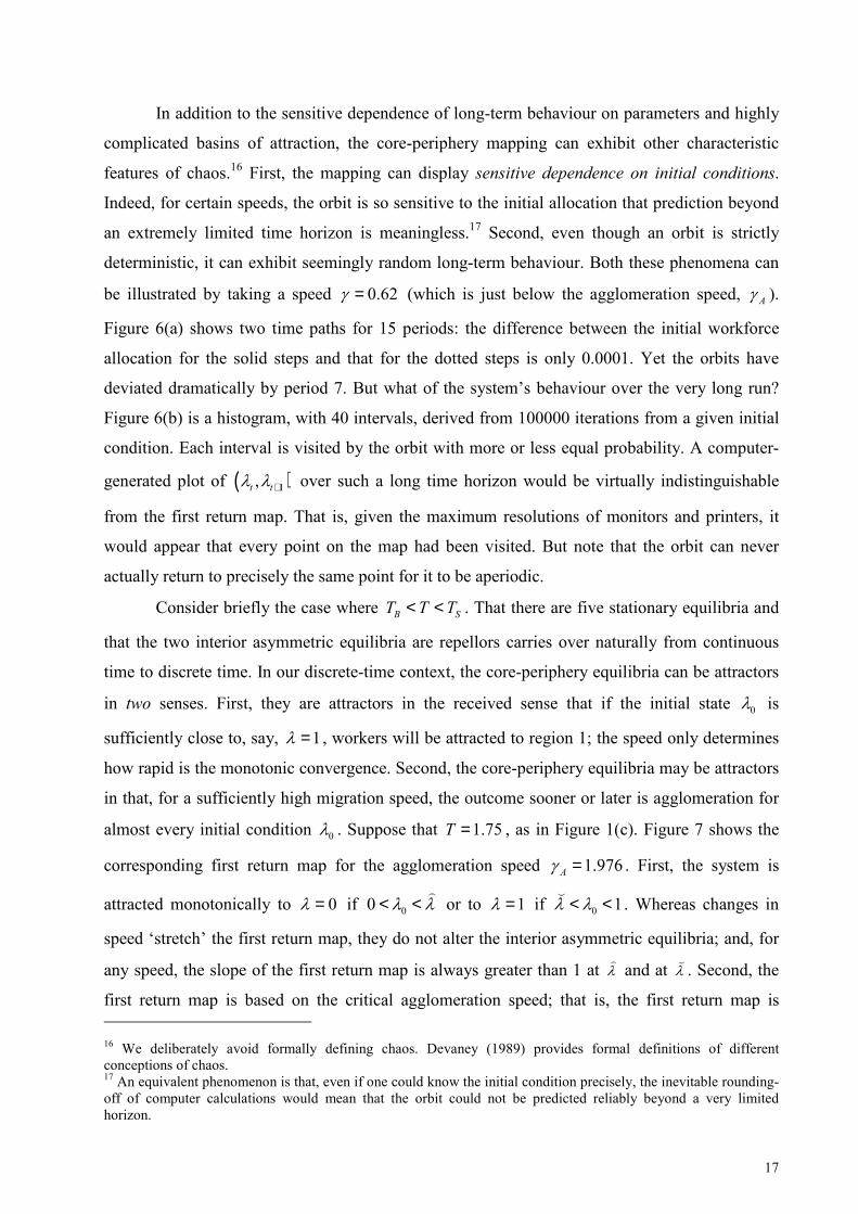
In addition to the sensitive dependence of long-term behaviour on parameters and highly

complicated basins of attraction, the core-periphery mapping can exhibit other characteristic

features of chaos.16 First, the mapping can display sensitive dependence on initial conditions.

Indeed, for certain speeds, the orbit is so sensitive to the initial allocation that prediction beyond

an extremely limited time horizon is meaningless.17 Second, even though an orbit is strictly

deterministic, it can exhibit seemingly random long-term behaviour. Both these phenomena can

be illustrated by taking a speed 0.62γ = (which is just below the agglomeration speed, Aγ ).

Figure 6(a) shows two time paths for 15 periods: the difference between the initial workforce

allocation for the solid steps and that for the dotted steps is only 0.0001. Yet the orbits have

deviated dramatically by period 7. But what of the system’s behaviour over the very long run?

Figure 6(b) is a histogram, with 40 intervals, derived from 100000 iterations from a given initial

condition. Each interval is visited by the orbit with more or less equal probability. A computer-

generated plot of ( )1,t tλ λ + over such a long time horizon would be virtually indistinguishable

from the first return map. That is, given the maximum resolutions of monitors and printers, it

would appear that every point on the map had been visited. But note that the orbit can never

actually return to precisely the same point for it to be aperiodic.

Consider briefly the case where B ST T T< < . That there are five stationary equilibria and

that the two interior asymmetric equilibria are repellors carries over naturally from continuous

time to discrete time. In our discrete-time context, the core-periphery equilibria can be attractors

in two senses. First, they are attractors in the received sense that if the initial state 0λ is

sufficiently close to, say, 1λ = , workers will be attracted to region 1; the speed only determines

how rapid is the monotonic convergence. Second, the core-periphery equilibria may be attractors

in that, for a sufficiently high migration speed, the outcome sooner or later is agglomeration for

almost every initial condition 0λ . Suppose that 1.75T = , as in Figure 1(c). Figure 7 shows the

corresponding first return map for the agglomeration speed 1.976Aγ = . First, the system is

attracted monotonically to 0λ = if 00 λ λ< <

or to 1λ = if 0 1λ λ< <

. Whereas changes in

speed ‘stretch’ the first return map, they do not alter the interior asymmetric equilibria; and, for

any speed, the slope of the first return map is always greater than 1 at λ

and at λ

. Second, the

first return map is based on the critical agglomeration speed; that is, the first return map is 16 We deliberately avoid formally defining chaos. Devaney (1989) provides formal definitions of different conceptions of chaos. 17 An equivalent phenomenon is that, even if one could know the initial condition precisely, the inevitable rounding-off of computer calculations would mean that the orbit could not be predicted reliably beyond a very limited horizon.

0 1

rela

tive

frequ

ency

(b)

Figure 6

1

0

tλ

time

(a)

7

Figure 7

λ

λ 10

1

tλ

1tλ +

18

tangent to the dotted square box formed by taking the unstable equilibria as its opposite corners.

For speeds below Aγ , if tλ is in ( ),λ λ

then so is 1tλ + and the orbit remains in ( ),λ λ

for all

subsequent time. In contrast, for speeds above Aγ , the first return map extends outside the box

and, sooner or later, agglomeration in one of the regions occurs for almost all initial conditions.

The case where BT T< can be dealt with even more briefly. Of the three fixed points, the

symmetric equilibrium is a repellor and the system converges monotonically on 0λ = if

0 0.5λ < and on 1λ = if 0 0.5λ > . The migration speed only impacts on the rapidity of

convergence.

Transport costs

Given the attention devoted by core-periphery theorists to the impact of changes in transport

costs, we now consider more directly the implications of changing T. Figure 8, based on 5σ = ,

0.4µ = , 100L = and 0.8γ = , shows the first return maps at 1.63 BT≈ ; at 1.742 PT≈ , the value

of T at which the period-doubling first occurs; at 1.81 ST≈ ; and at 1.924 AT≈ , the value of T

above which agglomeration is inevitable. Since ( ) 1M λ′ = + at BT , a subcritical pitchfork

bifurcation occurs as T increases through BT (as in the continuous-time model). Figure 9(a), a

bifurcation diagram for 0 0.51λ = , confirms that the symmetric equilibrium becomes unstable as

T increases through PT ; that further increases, which stretch the first return map, are broadly

‘destabilising’; and that, for AT T> , the system is attracted to a core-periphery state

(notwithstanding that a core-periphery equilibrium would be unstable in a continuous-time

context since A ST T> implies P Cω ω> ). In contrast to the continuous-time model, it is not the

case that, for ‘high’ transport costs, the dispersion force that derives from the immobility of

farmers necessarily overwhelms the circular causation for agglomeration generated by the

forward and backward linkages. The dependence of long-term behaviour on the initial condition

is shown in Figure 9(b), where the curved boundaries of B′ and B′′ correspond to the unstable

branches in the tomahawk diagram. For combinations of T and 0λ in B′ and B′′ , the outcome is

agglomeration. The symmetric equilibrium is an attractor for ( )0,T λ in S. For ( )0,T λ in C, the

system exhibits periodic or aperiodic long-term behaviour. For ( )0,T λ combinations in A, the

dynamical process results in agglomeration but in which region is highly sensitive to the precise

combination.

BT

ST

tλ 1

1tλ +

1

Figure 80

0

AT

PT

BT PT AT

1

0

(a)

(b)

1

0

B'

S C A

B''

1 2λ =

1 2λ =

Figure 9

19

Using (28), one can obtain the locus of combinations of mobility speed and transport cost

at which the symmetric equilibrium bifurcates into a period-2 attractor. This is the curve PP in

Figure 10(a). The symmetric equilibrium is an attractor for combinations of γ and T below PP

provided that BT T> . The curve AA is the locus of combinations of γ and T above which the

outcome is agglomeration. As T falls towards BT , the corresponding period-doubling speed Pγ

tends to infinity, as does the agglomeration speed Aγ (which necessarily exceeds Pγ ). Looking

at this somewhat differently, for any BT T> , there is some sufficiently high speed that the

symmetric equilibrium becomes a repellor. Figure 10(a) provides further confirmation that, as

long as T remains above BT , reductions in T are broadly ‘stabilising’ in that they increase both

the range of migration speeds for which the symmetric equilibrium is an attractor and the range

of speeds for which agglomeration is not brought about by the volatility of the system’s

behaviour. If T does fall below BT , the symmetric equilibrium becomes unstable.

Utility parameters

Figure 10(b) shows the impact of a ceteris paribus change in the share of income devoted to

manufactures: with an increase in µ from 0.4 to 0.5, the break point increases from BT ′ to BT ′′ and

the ( ),T γ bifurcation locus shifts from the solid P P′ ′ curve to the dotted P P′′ ′′ curve. If

B BT T T′ ′′< < , the increase in µ would lead to a core-periphery outcome (as a continuous-time

analysis would conclude). However, provided that BT T ′′> , the increase in µ extends the range of

speeds for which the symmetric equilibrium is an attractor. An increase in the consumers’ taste

for variety – i.e., a reduction in σ – would have similar effects to an increase in µ.

Figure 11, based on T = 2, 100L = and γ = 0.2, shows the interaction between µ and σ.

The boundary between BH and B is defined by ( )1σ σ µ− = ; that between B and S is the locus

of ( ),µ σ combinations for which 2BT = from (24); that between S and C, derived from (28), is

the locus of ( ),µ σ combinations for which, given T and γ, a period-doubling bifurcation first

arises; and the dotted curve is the locus of ( ),µ σ combinations for which 2ST = from (25). For

( ),µ σ in BH, the no-black-hole condition is violated. In B, the symmetric equilibrium is

unstable and the system is attracted to a core-periphery equilibrium. In S, the system is attracted

to the symmetric equilibrium. In C, there is periodic or chaotic co-existence of manufacturing.

For ( ),µ σ in A, the system’s behaviour is sufficiently volatile that the outcome is a core-

BH

B

S

C

A

0.1 0.92

10

Figure 11µ

σ

0

mob

ility

spee

d

BT ′ BT ′′

P′′P′

Figure 10

P′′P′

TSTBT0

(a) (b)

P

AP

A

20

periphery equilibrium; the basins of attraction are necessarily fragmented.18 FKV (p.75) base

their conclusion that a core-periphery geography is less likely the lower µ and the higher σ,

solely on the observation that such changes increase the range of transport costs for which

BT T< . However, in a discrete-time context, a fall in µ or a rise in σ could change periodic or

chaotic coexistence, or even a stationary symmetric equilibrium, into a strict core-periphery

geography.

6. Amendments and Developments

Much of The Spatial Economy: Cities, Regions and International Trade involves developing the

basic core-periphery model. Our discrete-time model could be similarly extended to encompass,

say, more than two regions, differences in the sizes of the agricultural sectors, mobility of labour

between agriculture and manufacturing, or more realistic transport cost structures. Our present

purpose here is to allude very briefly to some more immediate possibilities.

A natural development of the present model would be to relax the assumption of the

instantaneous entry and exit of manufacturers and to assume that entry and exit occur in response

to realised profits. Puga (1999), in a continuous-time model, assumes that manufacturers enter

and exit in response to realised profits but that the movement of workers is ‘instantaneous’. In

discrete time, this would give a similar model to the one we have examined. Depending on the

speed of entry or exit, periodic or aperiodic coexistence would be feasible; ‘rapid’ entry and exit

could result in agglomeration via volatility. Much more interesting would be to suppose that not

only firm entry and exit but also worker migration take place at the transitions between periods.

The strict proportionality between the number of manufacturers in a region and the regional

workforce would be disrupted; the precise combination of speeds would be crucial.19

The appropriate treatment of expectations is typically a contentious issue in a dynamical

model and the assumption of myopic behaviour on the part of workers in the core-periphery

model has been subject to criticism. For our discrete-time model, it is unlikely that a cycle of

very low periodicity could persist for long, since workers would be extremely naïve to fail to

detect it. However, in the face of cycles of long periodicity or chaotic behaviour, the continued

18 The boundary between A and C was derived by simulations and, especially for lower ( ),µ σ combinations, is rather more ‘ragged’ than it appears from the diagram. 19 Currie and Kubin (2002) consider the dynamic implications for a Dixit-Stiglitz monopolistic competition of manufacturers taking production decisions and entry/exit decisions in the face of shifting and uncertain demands.

21

use of some myopic rule of thumb by workers would be much more understandable.20 Krugman

(1991c) raised the ‘history versus expectations’ issue and, in particular, explored the possibility

that agglomeration can be a self-fulfilling prophecy. That is, workers might migrate into the

region that initially has fewer workers because they expect other workers do the same. Baldwin

(2001) incorporates forward-looking expectations in the continuous-time core-periphery model

and concludes that the assumption of myopia is rehabilitated if migration costs are high but that

self-fulfilling prophesies can arise with low migration costs. Given the extreme sensitivity of

long-term behaviour to initial conditions (and to parameters) in a discrete-time framework, even

posing sharply the history-versus-expectations issue is likely to be problematic.

7. Some Concluding Comments

The standard continuous-time core-periphery model is often used to tell a ‘story’ about the

impact of falling transport costs.21 Initially, at a high T, economic activity is distributed between

the regions. As T falls through ST , a core-periphery pattern, once established, can be sustained.

As T falls through BT , the symmetry between the regions is necessarily disrupted. Two features

of the model have received particular attention. First, a small reduction in T through BT results in

catastrophic agglomeration, where the process of regional divergence, once started, feeds upon

itself. The second is locational hysteresis. As T falls through BT , if one region has a slightly

higher workforce, agglomeration will occur in that region; whereas “had the distribution of

population at that critical moment been only slightly different, the roles of the regions might

have been reversed” (Krugman 1991a, p. 487). Moreover, if B ST T T< < , the economy could

shift from a symmetric equilibrium to a core-periphery equilibrium as a result of a location

shock, and not move back again when the cause of the shock is removed.

What then are the implications for this story of formulating the core-periphery model in

discrete time? Altering solely the temporal framework dramatically enriches the possible

dynamical behaviours.22 Whereas interior asymmetric equilibria are necessarily unstable in a

continuous-time model, the asymmetric coexistence of manufacturing in the regions is possible

in a discrete-time model. Such asymmetric long-term coexistence may be periodic (but not of

period-1) or even aperiodic. Moreover, for a given speed, agglomeration can result not only at 20 Rosser’s (1999) survey of complex economic dynamics encompasses the treatment of expectations and provides relevant references. 21 Krugman and Venables (1995) is based on a closely related model. 22 Replacing (6) by a discrete-time counterpart of the FKV migration process would not alter our qualitative conclusions in any fundamental way.

22

‘low’ transport costs, i.e., for BT T< , but also at ‘high’ transport costs as the natural outcome of

volatility. It should be emphasised that asymmetric coexistence or agglomeration via volatility

are possible for precisely those parameter combinations that core-periphery theorists have

deemed worthy of close scrutiny. Indeed, for any combination ( ), ,T µ σ such that BT T> , there

exist sufficiently rapid speeds (or sufficiently high numbers of workers) that periodic or chaotic

coexistence occur or for which agglomeration is the outcome of volatility.

Catastrophic agglomeration also occurs in the discrete-time model if T falls through BT .

More significantly, the sensitive dependence of long-term behaviour on parameters – and the

implied structural instability – is pervasive for BT T> . A miniscule change in a parameter can

abruptly change long-term behaviour from aperiodic or from a cycle of very long periodicity to,

say, a period-4 cycle. In addition, for the core-periphery mapping, a period-2 cycle can abruptly

bifurcate into three period-doubling cycles, two of which are attractors. The phenomenon of

hysteresis is also endemic in the discrete-time core-periphery model. Not only can our core-

periphery mapping exhibit the sensitive dependence on initial conditions that characterises

chaotic orbits. More significantly, there can be more than one attractor for given parameters,

with each attractor possessing a highly complex basin of attraction. This necessarily applies

where agglomeration is the outcome of volatility; in this event, which region becomes the core is

never a simple matter. More remarkably, at parameters for which there is periodic coexistence,

there can be two attractors with extremely complicated basins of attraction.

The rationale for telling the standard story is that various technological improvements

have brought secular reductions in transport costs. But there have also been significant changes

over time in the ease with which workers can move between regions and in their propensity to do

so in response to economic incentives. Whereas the standard continuous-time core-periphery

model can offer no insights into these latter questions, the importance of worker migration

speeds emerges inexorably from a discrete-time analysis. Of course, to explore the empirical

question of how rapidly workers do migrate – whether between regions within the same country,

between the member countries of the European Union, or between the ‘north’ and the ‘south’ –

is beyond the scope of the present paper.

The standard core-periphery model is sometimes labelled as being essentially ‘static’

equilibrium economics. We do not subscribe to this view. The identification of break and sustain

points in the tomahawk diagram and the associated analysis of centripetal and centrifugal forces

provide genuine dynamical insights. Moreover, one of Krugman’s significant contributions has

been to persuade more mainstream economists to take seriously the possibility of multiple

23

equilibria and to recognise that ‘history matters’. Nevertheless, formulating the model in discrete

time does bring dynamical considerations to the forefront. Moreover, in a discrete-time

formulation, the sensitive dependence of long-term behaviour on parameters and on initial

conditions is so acute and so pervasive that it must call into question reliance on the propositions

derived from the standard continuous-time model. The conclusions of our analysis are therefore

fully consonant with the conclusion of Neary (2001) that “the key problem is that the policy

implications of the basic core-periphery model are just too stark to be true”, and, in particular,

with his cautions against using the clear welfare-ranking that emerges from the simple model – it

is best to live in the core, next best to live in a diversified economy and worst to live in the

periphery – as the basis for a government role in ‘picking equilibria’.

Appendix 1: Sharkovskii’s Theorem

Central to the Theorem is the Sharkovskii ordering of the positive integers: 2 2 2 3 23 5 7 2 3 2 5 2 7 2 3 2 5 2 7 2 2 2 1¬ ¬ ⋅ ¬ ⋅ ¬ ⋅ ¬ ⋅ ¬ ⋅ ¬ ⋅ ¬ ¬ ¬ ¬ ¬ ¬

where m n¬ signifies that m appears before n in the ordering. That is, first come the odd integers

except 1; then 2 times the odd integers except 1; then 22 times the odd integers except 1; then…;

then the powers of 2 in decreasing order; and finally 1. Since every positive integer can be

written as 2k times an odd integer, for a suitable non-negative integer k and a suitable odd

integer, it does order all positive integers. We can now state:

Theorem

Suppose a continuous map of the real line has a periodic orbit of period p. If p appears

before some other positive integer q in the Sharkovskii ordering, then the map also has a

periodic orbit of period q.

Sharkovskii’s Theorem generalises the well-known Li-Yorke Theorem that the existence of a

period-3 orbit implies that there are periodic orbits of every other period. Since Sharkovskii’s

Theorem does not require that the mapping be unimodal, it applies to our core-periphery

mapping. For the latter, the significance of the Theorem is that, since 6 is the first integer in

the ordering after the listing of the odd numbers, the presence of a period-6 cycle [recall

Figure 3(c)] implies that the mapping has periodic orbits of every integer period following 6

in the ordering, i.e. for every positive even integer.

Figure 12

(a)

(b)

(c)

0 0 1tλ

2tλ +

1

0

2tλ +

1

0

2tλ +

1

1

1

0

0

tλ

tλ

24

Appendix 2 Bifurcation at γ *

Recall Figure 3(b), the first return map for a speed 0.3γ = , for which the attracting period-2

orbit involves cycling between λ′ and λ′′ . Figure 12(a) shows the corresponding second return

map, [ ] ( )22t tMλ λ+ = . Figure 12(b) shows the second return map at the critical speed,

* 0.3688γ ≈ , at which the period-2 cycle becomes unstable and the two new attracting period-2

cycles emerge. Note that, at the relevant intersections with the 450 line, the slope of the second

return map is +1. Increasing the speed above *γ creates 4 additional intersections, as in Figure

12(c), which is based on a speed 0.44γ = .

References

Baldwin, Richard E. (2001). The core-periphery model with forward-looking expectations.

Regional Science and Urban Economics 31: 21-49.

Currie, Martin and Ingrid Kubin (2002). Complex dynamics in monopolistic competition,

University of Mainz, Working Papers in Economics, 02-01.

Devaney, Robert L. (1989). An Introduction to Chaotic Dynamical Systems. Second edition.

Menlo Park, California: Addison-Wesley.

Dixit, Avinash K. and Joseph E. Stiglitz (1977). Monopolistic competition and optimum product

diversity. American Economic Review 67: 297-308.

Fujita, Masahisa, Paul R. Krugman and Anthony J. Venables (1999). The Spatial Economy:

Cities, Regions and International Trade. Cambridge: MIT Press.

Krugman, Paul R. (1991a). Increasing returns and economic geography. Journal of Political

Economy 99: 483-499.

Krugman, Paul R. (1991b). Geography and Trade. Cambridge: MIT Press.

Krugman, Paul R. (1991c). History versus expectations. Quarterly Journal of Economics 106(2):

651-667.

Krugman, Paul R. and Anthony J. Venables (1995). Globalization and the inequality of nations.

Quarterly Journal of Economics 110(4): 857-880.

Lorenz, Hans-Walter (1989). Nonlinear Dynamical Economics and Chaotic Motion. Berlin

Heidelberg: Springer-Verlag.

May, R.M. (1976). Simple mathematical models with very complicated dynamics. Nature 261:

459-467.

25

Neary, J. Peter (2001). Of hype and hyperbolas: Introducing the new economic geography.

Journal of Economic Literature 39(2): 536-561.

Ottaviano, Gianmarco I.V. and Diego Puga (1998). Agglomeration in the global economy: A

survey of the ‘new economic geography’. The World Economy 21(6): 707-731.

Puga, Diego (1998). Urbanization patterns: European versus less developed countries. Journal of

Regional Science 38(2): 231-52.

Puga, Diego (1999). The rise and fall of regional inequalities. European Economic Review 43(2):

303-34.

Robert-Nicoud, Frederic (2002). The structure of simple ‘New Economic Geography’ models.

Discussion paper. London School of Economics.

Rosser, J. Barkley, Jr. (1999). On the complexities of complex economic dynamics. Journal of

Economic Perspectives 13(4): 169-192.