core structure constraints david allan … because pmkp waves do not bottom in the upper regions of...
TRANSCRIPT
CORE STRUCTURE CONSTRAINTS
DERIVED FROM SKS AND SKKS OBSERVATIONS
by
DAVID ALLAN REED
B.S., MICHIGAN STATE UNIVERSITY (1968)
SUBMITTED IN PARTIAL FULFILLMENT
OF THE REQUIREMENTS FOR THE
DEGREE OF MASTER OF SCIENCE
at the
MASSACHUSETSS INSTITUTE OF TECHNOLOGY
NOVEMBER, 1973 .6. 3 /97
Signature of Autho
Department of Earth and Planetar Sciences, November 1973
Certified by
Thesis Supervisor
Accepted by
Chairman, Departmental Graduate Committee
CORE STRUCTURE CONSTRAINTS
DERIVED FROM SKS AND SKKS OBSERVATIONS
by
DAVID ALLAN REED
Submitted to
the Department of Earth and Planetary Sciences
November 1973
in partial fulfillment of the requirements of the degree
of Master of Science
ABSTRACT
We have made an extensive study of SmKS arrivals in
order to 1) examine the transmission and reflection response
of the core-mantle boundary and 2) constrain the velocity
structure of core regions in which PmKP waves do not bottom.
The SmKS data set included measurements of SKS/SKKS amplitude
ratios, SKKS phase lags (relative to SKS), travel times and
dT/dA values. In addition to long period data, we have measured
over 500 short period travel times corresponding to SKS, SKKS,
and SKKKS. SKKKS-SKKS and SKKS-SKS travel time differences have
also been employed in this study.
We have isolated an SKS/SKKS amplitude ratio minimum and
a region of phase shifts in our data for epicentral distances
of 109*-110*. We find that these observations are associated

ii
with the transmission of SKS through the core-mantle boundary
and that as a consequence, the SKS p-A curve is constrained
to pass through the mean value of wave slowness for diffracted
P (~ 4.55 sec/deg) between distances of 1094 and 1100. Once
the SKKS internal caustic is taken into consideration, we
find that theoretical transfer functions for a sharp core-
mantle boundary model similar to the B2 model of Bullen and
Haddon (1967) provide a reasonable fit to our amplitude ratio
and phase lag data. We also find that the SKS/SKKS amplitude
ratios exhibit a negligible dependence on frequency, and
that if present, core-mantle boundary layering is probably
less than about 10 to 15 kilometers in extent.
The second part of this thesis delineates the results
from our study of the outer core velocity structure. We
derive a velocity model (SKORl) for the outer core and dis-
cuss the fit of this model to our SmKS travel times and dT/dA
values as well as the 1968 Herrin times for PKP. The outer
600 kilometers of SKOR1 were constrained by our SKKS dT/dA
values as well as SKKS, SKKKS, SKKKS-SKKS and SKKS-SKS travel
time data. We find that the P wave velocity at the core mantle
boundary is about 8.015 km/sec and that it increases at a
nearly constant rate of about -0.00155 sec~1 throughout the
outer 250 kilometers of the core. However, the velocity
gradient changes to a value of about -0.0022 sec~1 between
radii of 3050 and 3250 kilometers, and this change is re-
flected in our amplitude and dT/dA data.
iii
The remaining portions of SKORl were constrained by
SKKS-SKS time differences and by the absolute times of the
SKS first arrivals (usually referred to as the AC branch).
We find that SKOR1 possesses a positive perturbation in
velocity (relative to other recent core models) centered at
a radius of about 2500 kilometers. This features is very
similar to the results given in the Bl model of Jordan (1973).
The improved resolution of the SmKS arrivals provided by our
short period data has resulted in initial evidence for addi-
tional SKS travel time branches. We are currently under-
taking an analysis of a combined PmKP and SmKS data set in order
to obtain a consistent explanation for these "secondary"
arrivals.
Acknowledgements
The results presented in this thesis would not have been
possible without the help of many friends. To name them all
seems like a formidable task. I am particularly grateful
to Professor Keiiti Aki for originally suggesting study
of SmKS arrivals, to Dr. Clint Frasier for the many hours
which he spent helping me with the core-mantle boundary
portion of this thesis, and to Professor M. Nafi Toksoz
for his guidance of my efforts to determine the velocity
structure of the outer core. I would also like to thank
Dr. Bruce Julian, Dr. Anton Dainty, Ken Anderson and Robert
M. Sheppard for making their computer programs available to
me, Russ Needham and Larry Lande for showing me how to interpret
seismograms and to Dr. David Davies, Dr. John Filson and
Raymon Brown for their suggestions throughout the course of
this study. The presentation of this thesis was greatly
expedited because of the help that I received from Dorothy
Frank and Carol Van Etten in typing the manuscript. The
long hours spent by these two people is deeply appreciated.
The time spent in preparing a thesis can sometimes
produce a significant burden on the human spirit. For this
reason, I feel a need to express gratitude for the patience,
encouragement, understanding, and above all, friendship of
Professor M. Nafi Toksoz, Dr. Clint Frasier, Raymon Brown,
Sara Brydges, Ben Powell, Mary Laulis and my psychiatrist.

V
This research was sponsored by the Air Force Cambridge
Research Laboratories, Air Force Systems Command under
Contract F19628-72-C-0094

Table of Contents
gaqsAbstract
Acknowledgements IV
Table of Contents Vi
Chapter 1 Introduction 1
Tables and Figures 4
Chapter 2 Sources and Analysis of Data
2.1 Data Source 7
2.2 Signal Travel Time and dT/dA Analysis 8
2.3 Signal Amplitude Analysis 9
2.4 Signal Phase Analysis 10
Figures 14
Chapter 3 Study of the Core-Mantle Boundary 22
3.1 Data Base for the CMB Study 23
3.2 Interpretation of the CMB Data Base 25
3.3 Conclusions from the CMB Study 30
Tables and Figures 32
Chapter 4 Inversion of the Outer Core Velocity Structure
4.1 Constraints on the Velocity Structure for 51the outer 600 kilometers of the core
4.2 Analysis of Core Model SKOR1 56
4.3 Evidence for Additional SKS Travel Time 59Branches
4.4 Conclusions from the Outer Core VelociLy 60Study
Tables and Figures 62
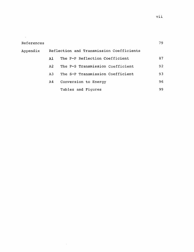
References
Appendix Reflection and Transmission Coefficients
Al The P-P Reflection Coefficient
A2 The P-S Transmission Coefficient
A3 The S-P Transmission Coefficient
A4 Conversion to Energy
Tables and Figures
vii
87
92
93
96
99

1. Introduction
Improvements in instrumentation and technique developed
in the past decade have been largely responsible for an
increasing number of seismic wave studies aimed at refining
the early core models of Jeffreys (1938, 1939a, 1939b),
Gutenberg and Richter (1934, 1935, 1946, 1939) and Gutenberg
(1958). Most of these refinements have been based on
studies of short period core arrivals which propagate through
the mantle in the longitudinal mode. Seismic waves used for
this purpose include PmKP (m = 1 through 9), PKIKP, PKiKP and
PKJKP (Adams and Randall, 1964; Bolt, 1964, 1970; Ergin, 1967;
Shurbet, 1967; Engdahl, 1968; Shahidi, 1968; Bolt and Qamar,
1970; Engdahl et al., 1970; Buchbinder, 1971; Adams, 1972;
Yanovskaya, 1972; Jordan, 1973; Qamar, 1973; Toksoz et al.,
1973). However, all of these studies are biased towards con-
straining core models at depths greater than about 3900 kilo-
meters, because PmKP waves do not bottom in the upper regions
of the outer core. This bias has resulted in a deficiency
of the high quality data prerequisite to a better understanding
of the core at depths less than 3900 kilometers. Indeed,
complete characterization of the outer core is particularly
germane to the questions of core formation and generation of
the carth's magnetic field.
ThLs thesis presents original data and preliminary
intierpretations of SmKS waves (multiply reflected core

arrivals which propagate through the mantle in the trans-
verse mode) which have been examined in order to: 1) deter-
mine their usefulness for constraining core-mantle boundary
(CMB) models; 2) constrain core regions in which the PmKP waves
do not bottom; and 3) test models derived to explain PmKP
observations (this is possible, because PmKP and SmKS waves
sample overlapping regions of the core). Typical SKS and SKKS
ray paths shown in Figure 1.1 (Toksoz et al.; 1973) indicate
that study of SKKS arrivals is well suited for constraining
the upper 600 kilometers of the core (since S interferes with
SKS at distances less than 85*), while study of SKS arrivals
provides us with the desired constraints for outer core regions
at radii less than approximately 3000 kilometers.
Recently, several core studies employing SKS and SKKS
observations have appeared in seismological literature. The
data employed in these studies included travel times (Hales
and Roberts, 1970, 1971a, 1971b; Randall, 1970) and dT/dA values
(Toksoz et al., 1973; Wiggins et al., 1973) measured on seis-
mograms from long period horizontal component instruments.
However, we believe that the long period nature of these waves
(typically 15 to 30 seconds) has limited their usefulness for
detecting fine structure in the earth's outer core. The
approach taken in this investigation presents two main advan-
tages over those previously used for SmKS study:
1) the data set includes many short period SKS and SKKS
observations which provide improved resolution of travel

3
times at closer distances and of additional SKS branches
and; 2) travel times have been combined with dT/dA measure-
ments, SKS/SKKS amplitude ratios and SKS-SKKS phase lags in
order to obtain a consistent understanding of model constraints.
The second chapter of this thesis describes the tech-
niques which we have employed for data collection and analysis,
while the remaining chapters delineate our interpretations of
the SmKS data set. Results from the core-mantle boundary
study are presented in chapter 3. Chapter 4 describes our
base model for the outer core, and the fit of this model to
SmKS and PKP travel times. The fourth chapter also contains
a description of some initial evidence for SKS "secondary"
arrivals which may imply the necessity for future pertur-
bations to our base model at radii less than about 2700
kilometers.
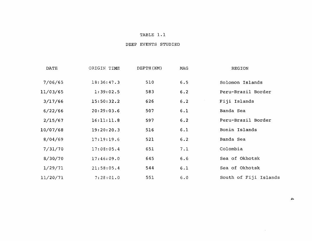
TABLE 1.1
DEEP EVENTS STUDIED
DATE
7/06/65
11/03/65
3/17/66
6/22/66
2/15/67
10/07/68
8/04/69
7/31/70
8/30/70
1/29/71
11/20/71
ORIGIN TIME
18:36:47.3
1:39:02.5
15:50:32.2
20:29:03.6
16:11:11.8
19:20:20.3
17:19:19.6
17:08:05.4
17:46: 09.0
21:58:05.4
7: 28 :01.0
DEPTH(KM)
510
583
626
507
597
516
521
651
645
544
551
MAG
6.5
6.2
6.2
6.1
6.2
6.1
6.2
7.1
6.6
6.1
6.0
REGION
Solomon Islands
Peru-Brazil Border
Fiji Islands
Banda Sea
Peru-Brazil Border
Bonin Islands
Banda Sea
Colombia
Sea of Okhotsk
Sea of Okhotsk
South of Fiji Islands

FIGURE CAPTIONS
Figure 1.1 SKS and SKKS ray plots for the core model
of Toksoz et al. (1973) showing the SKKS
internal caustic and SKS focusing.

I 38nouI
2. Sources and Analysis of Data
2.1 Data Source
The results presented in this study are based on
original data extracted from SmKS waveforms and travel times.
The SKS and SKKS observations utilized in constructing this
data base came from three sources: 1) long period WWSSN
seismograms for 1970 and 1971 M b>6.0 events; 2) LASA and
NORSAR data tapes from 1965 to 1973; and 3) long and short
period WWSSN seismograms for the 11 deep events listed in
Table 1.1. Although thousands of seismograms were examined.
during this study, we choose to limit our data base to
approximately 700 high quality SKS, SKKS and SKKKS arrivals.
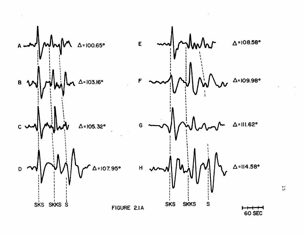
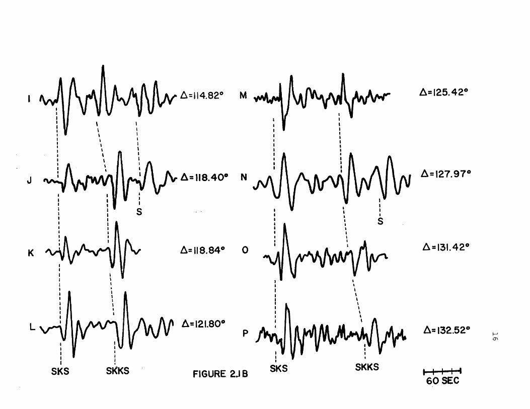
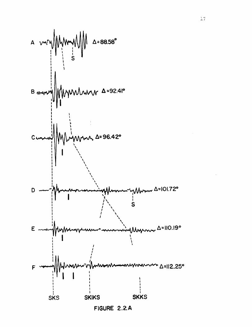
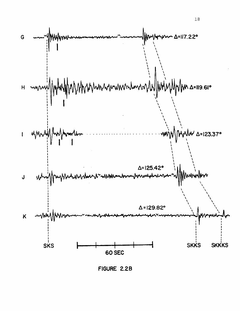
Examples of these arrivals are shown in Figures 2.1 (long
period) and 2.2 (short period).
Most of the data employed in this study fall within
the distance range 85*<A<135*. The lower limit is imposed
by the condition that S, SKS and SKKS travel times inter-
sect near this distance making signal separation difficult
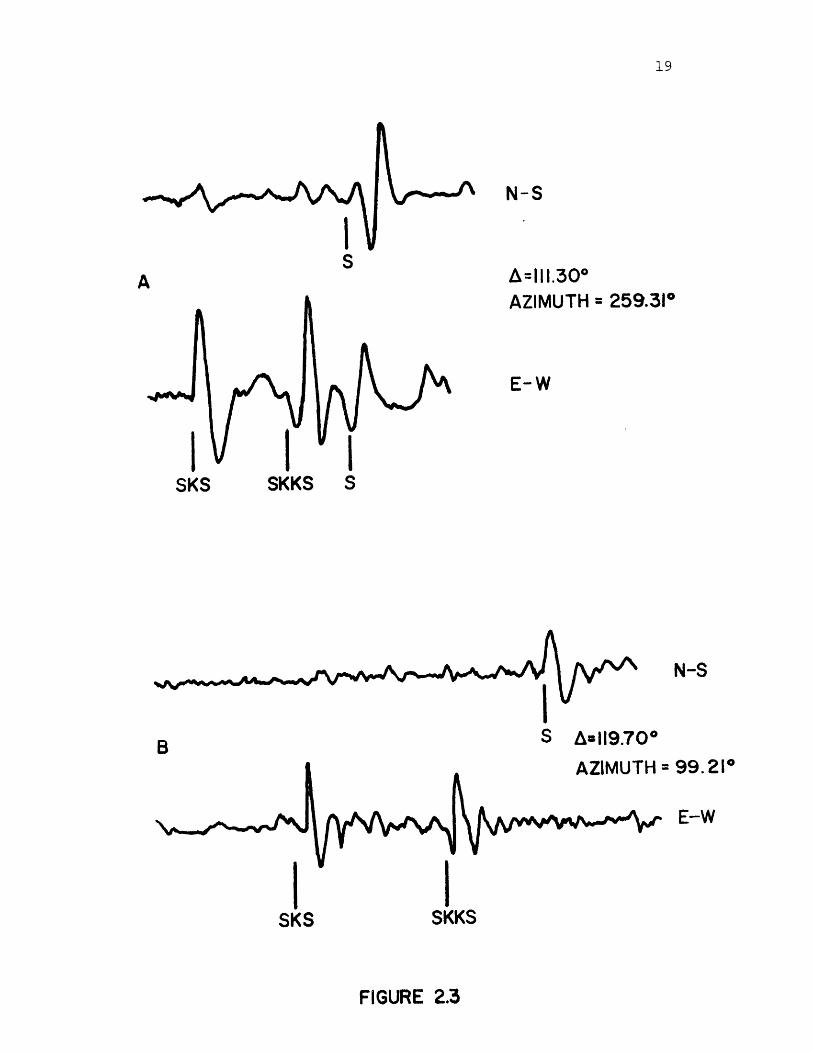
for A<85*. We found that signal polarization provided a
useful tool for separating S and SmKS arrivals. Continuity
cf particle velocity at the core-mantle boundary requires
IV-polarization of SmKS arrivals (assuming zero core rigidity).
Although observed SKS and SKKS arrivals are not of pure SV-
mode, they are very nearly so as shown in the examples of
Figure 2.3.
Consequently, when possible we compared SKS/SKKS amplitude
ratios for both NS and EW components in order to avoid the
mistake of incorporating S waves into our data. This approach
is particularly effective at distances greater than about 1000,
because diffracted S waves are primarily polarized in the SH-
mode (Cleary, 1969). The upper distance limit has been imposed
by our desire to concentrate primarily on the outer core and
core-mantle interface. Consequently, only a limited number of
travel times have been measured for distances greater
than 1350.
2.2 Signal Travel Time and dT/dA Analysis
2.2.1 SKS and SKKS travel times.
Examination of seismograms for the deep events
listed in Table 1.1 provided approximately 500 short period SKS
and SKKS signals for which accurate arrival times could be
obtained. These data were supplemented with arrival times
from selected long period WWSSN seismograms which exhibited
clear signal onsets. We found that it was particularly
difficult to determine SKKS arrival times, because their onsets
are not sharp as in the case of SKS. This problem is due to
the fact that SKKS is not a minimum time path arrival (note
the SKKS internal caustic in Figure 1.1; Shimamuro and Sato,
1965; Jeffreys and Lapwood, 1957), All arrival times were
converted to travel times using NOAA source parameters
and recorded to the nearest 0.1 second. Distances and
azimuths were computed for each event-station pair
using a program provided by Mr. R.M. Sheppard. The
travel time versus distance data set was next corrected
for depth of focus (correction to 33 kilometers) using
the Jeffreys-Bullen Tables (Travis, 1965) and for earth
ellipticity using the ellipticity tables of Bullen (1939).
Errors present in our final travel time versus
distance table come from several sources: 1) origin time
errors; 2) event location errors; 3) onset measurement
errors; and 4) errors inherent in the models used for
depth of focus and ellipticity corrections. We estimate
that SKS travel times have an accuracy of ± 1.0 second
and ± 0.2 seconds for the long and short period arrivals
respectively, while the error limits for SKKS arrivals
are approximately twice these values.
2.2.2 SKS and SKKS dT/dA values.
SKS and SKKS dT/dA values were measured using
the Data Analysis facilities of the Lincoln Laboratory
Seismic Discrimination Group. LASA and NORSAR long period
data tapes provided about 40 events for which SKS and/or
SKKS signals were easily identified. Time delays of these
signals at each array sensor location were converted to
horizontal phase velocities using the Data Analysis
subroutines. The reciprocals of these phase velocities
were then computed to obtain dT/dA values. We have
computed 95% confidence limits for these measurements
using the formula given in equation 2.1 (Kelley, 1964):
Y = (6/N)1/2 (TC/L) 2.1
where a = standard deviation, N = number of sensors used,
T = RMS time error of plane wave fit, L = array aperature
and C = expected phase velocity.
2.3 Signal Amplitude Analysis
Except for LASA and NORSAR arrivals, all amplitudes
used in this study were measured on 15X enlargements of
70 mm film chips for the WWSSN seismograms. Only those
long period seismograms which showed SKS and SKKS arrivals
with signal to noise ratios greater than about 5 were
subjected to amplitude analysis. We also chose to use
only a limited number of short period SKS and SKKS arrivals
for amplitude study, because these waves have periods which
fall on steep portions of the WWSSN instrument magnification
curves making corrections difficult.
Peak to peak amplitudes of the SKS and SKKS arrivals
were measured with an accuracy of ±0.2 mm. Since the long
period arrivals used had paper record amplitudes greater

than 20 mm, measurement errors are estimated to be less
than 2%. Short period signal amplitudes could be in
error by as much as 10%. Measured amplitudes were
corrected for instrument magnification using WWSSN
magnification curves and the signal frequency of peak
power obtained from spectral analysis. Corrections for
azimuthal direction of the incoming waves were applied
under the assumption of SV-polarization. Finally, we
chose to normalize all amplitudes to a NOAA magnitude
of 6.5 Mb by multiplying them by the factor 10AMb, where
AMb equals 6.5 minus the NOAA event magnitude.
2.4 Signal Phase Analysis.
In order to avoid the complication of calculating
source radiation patterns for all of the events studied,
we chose to examine the phase difference of SKS and SKKS.
At first, this phase difference was determined using the
imaginary and real parts of the SKS/SKKS spectral ratio.
We found, however, that phase spectra obtained in this
way were oscillatory and difficult to interpret. Consequently,
we decided to employ a technique of phase shift filtering
and signal correlation. This technique (performed on
the computing facilities of the Lincoln Laboratory Seismic
Discrimination Group) consisted of several steps: 1) The
record section containing SKS and SKKS signals for a given
event was displayed on a CRT facility with sampling at 1.0

second intervals; 2) A time window defined by the signal
frequency of peak power for the broadest of the two waves
was visually placed around each signal; 3) The SKS time
window was placed in a reference buffer, while the SKKS
time window was iteratively passed through a Hilbert
transform phase shift filter at 10 degree intervals. The
correlation coefficient of the SKS and SKKS time windows
was computed after each iteration; 4) This iteration was
repeated in 1 degree intervals over the 20 degree range
of best correlation, and the phase shift providing the
highest degree of correlation determined; 5) The SKS
and shifted SKKS signals were compared on the CRT facility
after the analysis to visually check our results.
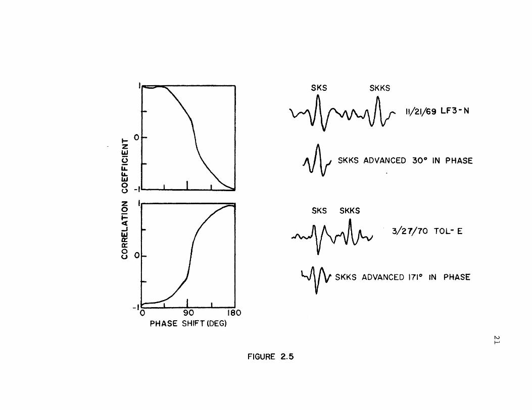
The phase shift and correlation technique utilized in
this study was made under the assumption that all frequencies
of the SKS and SKKS signals have been shifted through a
constant phase angle. Although this assumption is not
strictly true, we feel that the simple time domain shapes
of these waves combined with their rapid amplitude decay
away from the peak frequency of their power spectra indicates
that favoring this dominant frequency should provide a good
first approximation to the SKS-SKKS phase difference.
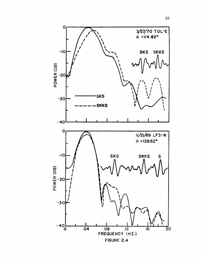
Ficure 2.4 illustrates typical SKS and SKKS record sections
and the corresponding power spectra, while Figure 2.5
shows several examples of the results from our phase shift
13
and correlation technique. The results shown in Figure 2.5
indicate that SKKS phase lags (relative to SKS) obtained
in this study have an accuracy of about ±15 degrees.

FIGURE CAPTIONS
Figure 2.1
Figure 2.2
Figure 2.3
Figure 2.4
Figure 2.5
Examples of long period SmKS arrivals:
A: 2/15/67 NUR-E; B: 6/5/70 ALQ-N; C: 2/15/67
HLW-E; D: 2/21/71 NOR-N; E: 4/20/70 KBL-E; F:
6/17/71 AAE-E; G: 4/16/70 AAE-N; H: 5/2/71 LPB-N;
I: 3/27/70 TOL-E; J: 5/2/71 ANT-N; K: 8/13/71
N4B-E; L: 4/16/70 NAI-N; M: 1/29/71 BUL-N; N:
11/21/69 LE4-N; 0: 1/29/71 ARE-N; P: 8/30/70 LPB-E.
Examples of short period SmKS arrivals:
A: 10/7/68 JER-E; B: 10/7/68 HLW-E; C: 1/29/71
AAE-N; D: 8/4/69 UME-E; E: 1/29/71 CAR-N; F:
1/29/71 BAG-N; G: 3/17/66 SJG-E; H: 11/20/71 KBL-E;
I: 8/4/69 GOL-E; J: 1/29/71 BUL-E; K: 1/29/71 PRE-N.
Seismograms showing SV-polarization of SKS and
SKKS. A: 2/21/71 NUR; B: 11/20/71 KBL.
Power spectra for typical long period SKS and
SKKS arrivals.
Determination of the SKKS phase lag (relative to
SKS) using the phase shift and correlation
method.
A= 100.65*
A=103.16*
=108.58*
A=109.98*
A=III.62*
A=114.58*
A= 105.32*
A=107.95*
y II II I II I I
I 1
SKS SKKS FIGURE 2.IA
IIIV
IV I
SKS SKKS
60 SEC
ii VB'' bI IIB IIB 11
B I* IB IB II IB B~A
I14.820
A:118.400
A= 118.840
A=121.80*
M
N
0
p
B B
I II B
IA a
B I
I IB IB IB a IIL
B II Iiii
A= 125.42*
A=127.97*
A=131.42*
A= 132.520
SK SK K
SKS SKKSFIGURE 2JB
60 SECSKS SKKS
A= 88.580
IiA =92.41*
C A=96.42*
D A=101.72*
E ~
I '4I I
I II II I
III Infl IA
L=110.19*
* A=112.25*Ii I
SKS SKIKS SKKS
FIGURE 2.2A
III 1I* -
lull,. 11'*ii II II II II II I
~ I\MLhNAAfA~w\4bvv~M
A=117.22*
k A=119.61*
IIII
II
I
A=123.37*
A= 125.42*
A= 129.820
K
I II II I
I j
SKKS SKKKSI I
60 SEC
FIGURE 2.2B
SKS :
N-S
A=111.30*AZIMUTH = 259.31*
E-W
SKKS S
(V'*' 1 N-S
A=119.70 0
AZIMUTH = 99.21*
%A E-W
ISI ISKS SKKS
FIGURE 2.3
A
ISKS
S-20
00.
-30
-40
0
-10
W- 2 0 -
00-
-30
-40.0 .04 .08 .12 16 20
FREQUENCY (HZ.)
FIGURE 2.4
SKKS
11/21/69 LF3 - N
SKKS ADVANCED 30* IN PHASE
SKS SKKS
3/27/70 TOL- E
0
0
-c 90 180PHASE SHIFT (DEG)
FIGURE 2.5
I I i
9 V SKKS ADVANCED 1710 IN PHASE
NW.W=Wmma
SKS
41

22
3. Study of the Core-Mantle Boundary
Recent studies of the core-mantle boundary (CMB)
have been based on PcP and ScS arrivals (Balakina et al.,
1966; Kanamori, 1967; Buchbinder, 1968; Vinnik and Dashkov,
1970; Ibrahim, 1971, 1973; Frasier, 1972; Kogan, 1972;
Berzon and Pasechnik, 1972; Bolt, 1972; Anderson and
Jordan, 1972), diffracted arrivals (Alexander and Phinney,
1966; Sacks, 1966, 1967) and free oscillations (Dorman
et al., 1965; Derr, 1969). Since the nature and extent
of any CMB layering is one of the issues still subject
to considerable debate, we examined the SmKS data set to
determine what information can be obtained from waves
which sample the transmission and reflection response of
this interface.
Figure 3.1 illustrates theoretical amplitude and
phase curves for the CMB transmission and reflection
response. We have calculated these curves using the B2
model of Bullen and Haddon (1967). CMB incidence angles
for SKS and SKKS (assuming the B2 model and the Jeffreys-
Bullen Tables -- Travis 1965) are shown in Figure 3.2.
This diagram indicates that SKKS transmits through the
CMB past the P-wave critical angle (2132.5*) for the
distance range 85*6A-135*. On the other hand, SKS
transmits through the CMB at angles less than critical
for distances greater than about 106*. As shown in

Figure 3.1, the passage of SKS through the CMB at
distances where this critical angle is reached should
produce a narrow amplitude minimum and region of phase
shift. Consequently, we isolate this feature in section
3.1 and then interpret our observations in terms of CMB
model studies in section 3.2.
3.1 Data Base for the CMB Study
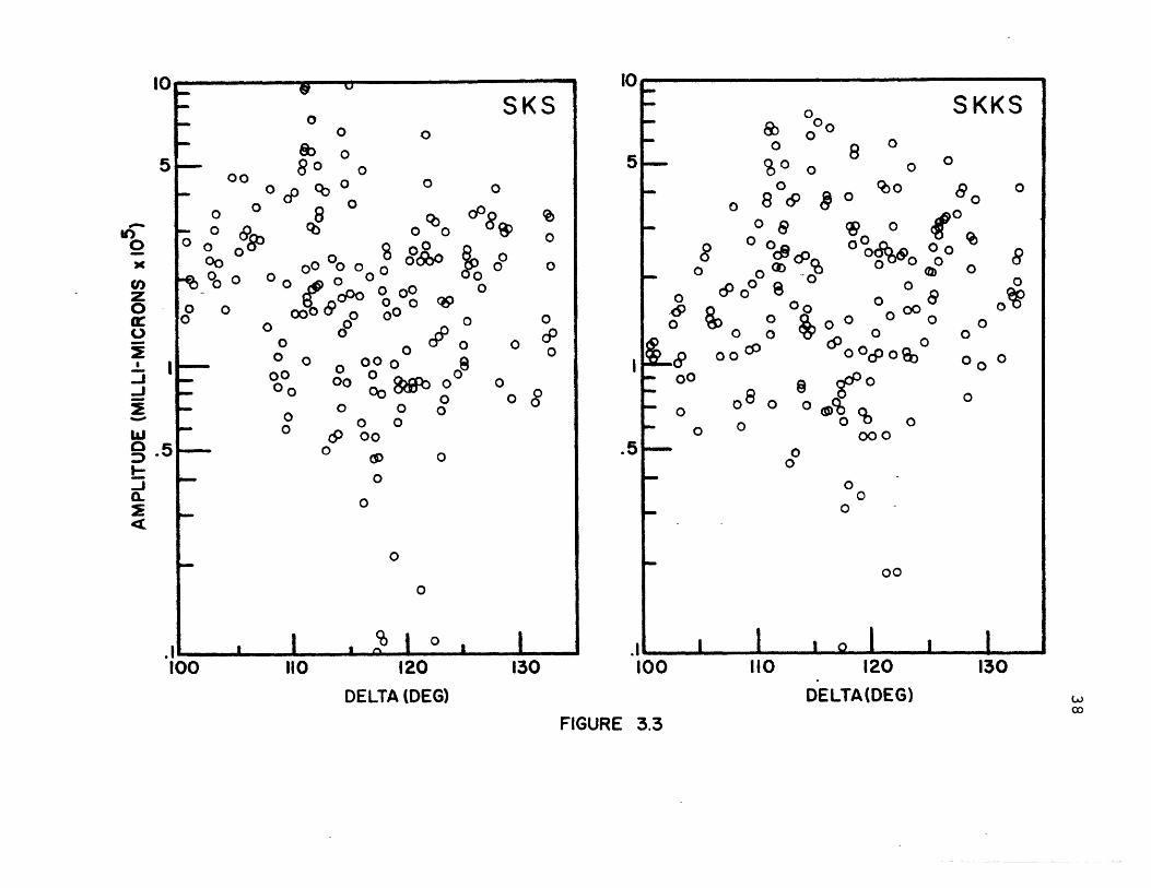
The observed long period SKS and SKKS amplitudes
(corrected for instrument magnification, azimuth and event
magnitude as described in section 2.3) are shown in Figure 3.3.
The scatter inherent in the present form of these data
prohibits their use for interpreting CMB properties.
However, valuable information can be extracted from the
SmKS data by using amplitude ratios (Kanamori, 1967), since
most of this scatter probably results from near source and
receiver effects. General expressions for observed SKS
and SKKS amplitudes are of the form:
A(f,A) = S(f,i,O) I(f,e,G) G(A) B(fA) D(f,A) 3.1
where S(f,i,O) is the source spectrum as a function of
frequency, take-off angle and azimuth; I(f,e,O) is the
instrument response spectrum as a function of frequency,
emergence angle and azimuth; G(A) is the geometrical

24
spreading factor; B(f,A) is the CMB response spectrum;
and D(f,A) is the attenuation spectrum given by
D(f,A) = exp(-t*f) 3.2
where t* =f ds3v (S) Q TT'S)
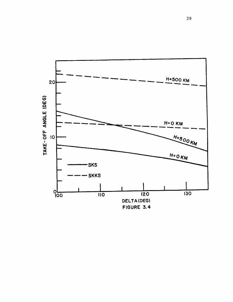
SKS and SKKS take-off angles are shown in Figure 3.4.
This diagram indicates that the upper mantle paths for
both wave types should be similar. Consequently, formation
of the amplitude ratio SKS/SKKS results in the approximate
cancellation of source and receiver uncertainties, and
hence a reduction in data scatter as shown in Figure 3.5.
We also show short period SKS/SKKS amplitude ratios in
this diagram for comparison, but these short period ratios
have not been corrected for any differences in frequency
content between SKS and SKKS.
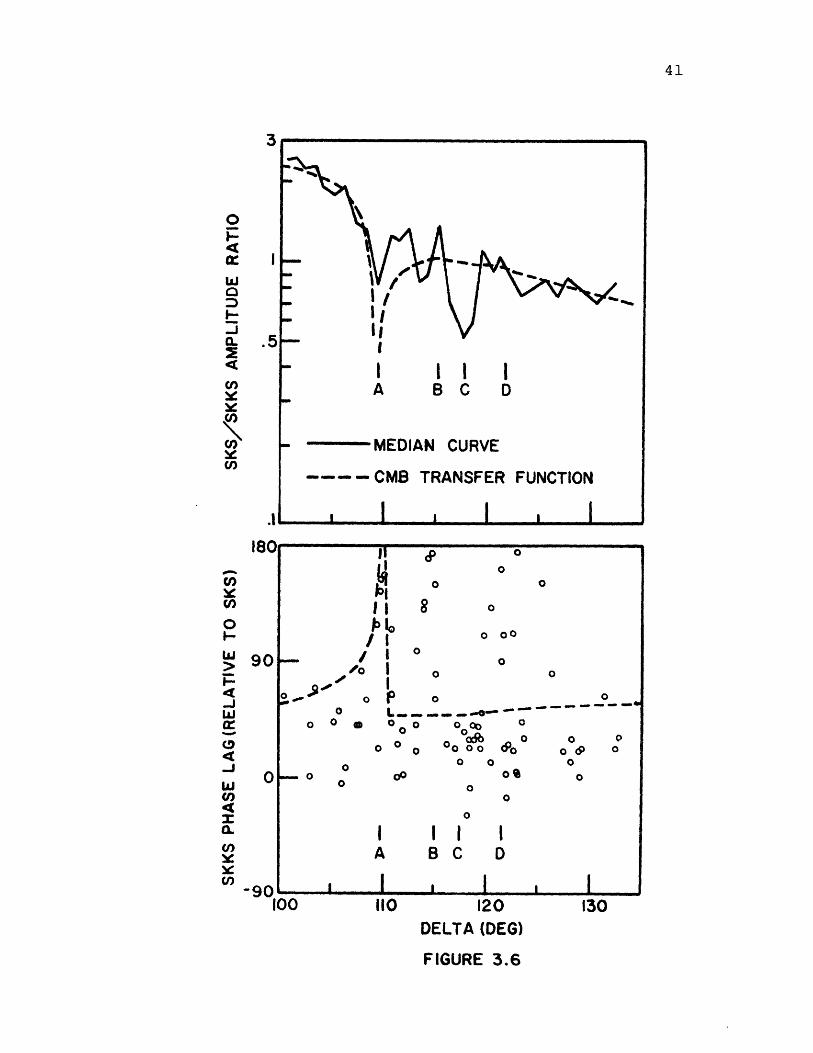
Figure 3.6 illustrates the correlation between
amplitude ratio and phase information derived from the
data set. The amplitude ratio portion of this diagram
was obtained by taking the median value of Figure 3.5 in
1.0 degree intervals for 100* A: 135*. We found no
evidence for an amplitude ratio minimum and phase shift
at A = 106*, but have isolated these features near
distances of 109*-110* (region A of Figure 3.6). Although

Figure 3.6 illustrates other regions (B through D) with
anomalous amplitude and phase values, we found that
these features occurred at distances which precluded
the possibility of their being an expression of CMB
transfer function effects. Consequently, we concentrate
on explaining region A in section 3.2 and then examine
the origin of features B through D in chapter 4.
3.2 Interpretation of the CMB Data Base
The results shown in Figure 3.1 as well as the
CMB model studies discussed in this section have been
calculated using the propagator matrix technique for
homogeneous plane layers (Thomson, 1950; Haskell, 1953,
1962; Gilbert and Backus, 1966). These results are
subject to our basic assumption of plane waves and layers.
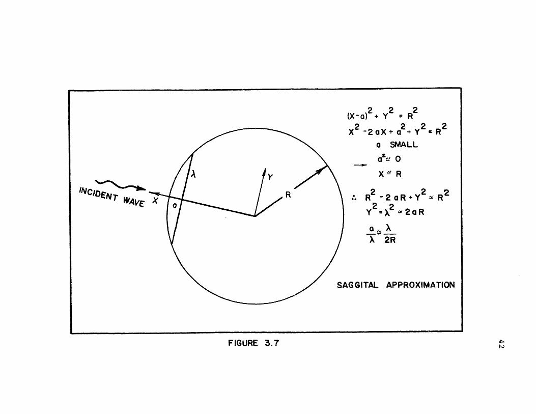
In order to evaluate the validity of assuming a plane
CMB, we invoked the Saggital Approximation for estimating
the effect of curvature (Born and Wolf, 1964). We find
that CMB curvature implies a/X ratios of 0.2% and 4% for
waves with periods of 1 and 35 seconds respectively (see
Figure 3.7 for nomenclature). Since the effect of
curvature is small for a/A ratios less than about 10%,
we conclude that the plane layer approximation should
not affect the basic results of this study.
Theoretical SKS/SKKS amplitude ratios and phase
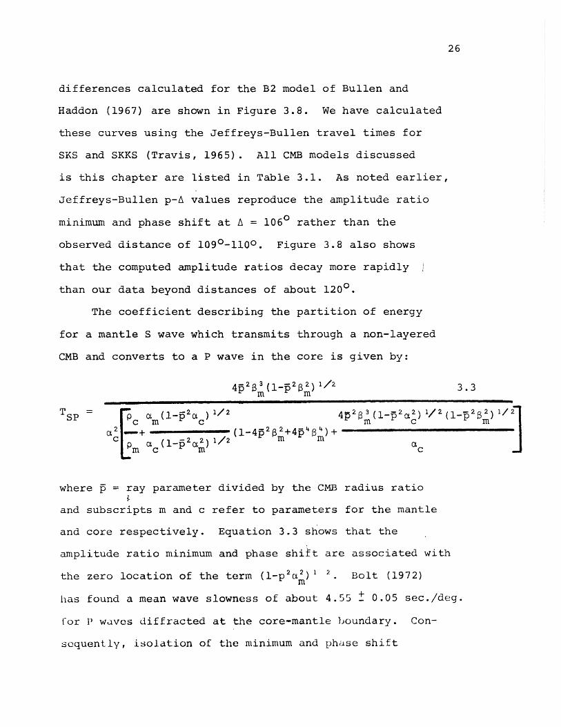
26
differences calculated for the B2 model of Bullen and
Haddon (1967) are shown in Figure 3.8. We have calculated
these curves using the Jeffreys-Bullen travel times for
SKS and SKKS (Travis, 1965). All CMB models discussed
is this chapter are listed in Table 3.1. As noted earlier,
Jeffreys-Bullen p-A values reproduce the amplitude ratio
minimum and phase shift at A = 1060 rather than the
observed distance of 1090-1100. Figure 3.8 also shows
that the computed amplitude ratios decay more rapidly
than our data beyond distances of about 1200.
The coefficient describing the partition of energy
for a mantle S wave which transmits through a non-layered
CMB and converts to a P wave in the core is given by:
4 p2 3 (1-p26 )21/2 3.3m m
TSP p a (1-p2a ) 1/2 4p2 3 (l_ 2 t2) 1/2 (1_p 2 2 ) 1/2
c m c m c maY'2 --AM+ (1-4p2 2+4pF)4 4)+
C[m mp a (1-f#2(2 21/2 m mX
m c m c
where p = ray parameter divided by the CMB radius ratio
and subscripts m and c refer to parameters for the mantle
and core respectively. Equation 3.3 shows that the
amplitude ratio minimum and phase shift are associated with
the zero location of the term (1-p2a2 )1 2 Bolt (1972)m
has found a mean wave slowness of about 4.55 t 0.05 sec./deg.
for 1 waves diffracted at the core-mantle boundary. Con-
sequently, isolation of the minimum and phase shift

associated with TSP near region A implies that the SKS
p-A curve goes through the value 4.55 ± 0.05 sec./deg.
at distances of about 109*-110*. We find that the
theoretical SKS p-A curve corresponding to our velocity
model SKOR1 (chapter 4) passes through this critical
value at distances of about 107.5*. This distance
is in reasonable agreement with the observed location
for feature A. Since a preliminary SKS p-A curve was
used in constructing model SKOR1, we anticipate an
improved fit to the location of feature A once this
curve has been constrained to fit all of the SKS
observations. Consequently, to aid comparison with
our data at this time, we have set am = 13.86 km./sec.
so that theoretical CMB transfer functions computed
using the present form of our p-A curves would pass
through the T5S minimum between 109* and 110*.
Substituting 13.86 km./sec. for a m, we have
recalculated the CMB transfer function for the B2 model
of Bullen and Haddon using the p-A curves corresponding
to model SKOR1. The results of this calculation are
compared to our mediap SKS/SKKS amplitude ratio curve
and SKS-SKKS phase lag data in Figure 3.6. The theoretical
phase lag curve shown in this diagram has been given a
90* correction to compensate for the SKKS internal
caustic. The agreement between theoretical and observed

data shown in Figure 3.6 is reasonably good. The improved
fit to observed amplitude ratio data beyond distances
of about 1200 is due to the incorporation of our SKKS
p-A values in these calculations (primarily because of
the high values of SKKS d 2T/dA2 for A = 115*-1200).
We next examined our ability to constrain a sharp
CMB model. We found that perturbations in ac and m by
more than about ± 0.3 km./sec. (relative to the values
for model B2) were required to produce transfer function
changes which exceeded the present scatter in our data.
We also calculated CMB transfer functions for several
recently published models (Balakina et al., 1966;
Buchbinder, 1968). The results of these calculations
are shown in Figure 3.9. This diagram indicates that
the addition of small amounts of outer core ridigity
produces only minor perturbations to models with yic = 0
(and hence S c = 0). Consequently, this study does not
allow us to place any constraints on this parameter. On
the other hand, theoretical amplitude ratios for the CMB
model proposed by Buchbinder (1968) do not fit our
observations. Buchbinder proposed this model
(characterized by a unity CMB density ratio and 7.5 km./
sec. value for ac ) to explain a PcP/P amplitude ratio
minimum and phase reversal near A = 32*. Our rejection
of this model is in agreement with the results of Frasier
(1972), Berzon and Pasechnik (1972), Kogan (1972) and
Chowdhury and Frasier (1973) which indicate that the
PcP/P amplitude ratio minimum and phase reversal do not
exist, but that the first PcP extremum is often buried
in noise near A = 32* making phase determination difficult.
Having completed our study of sharp CMB models, we
examined theoretical transfer functions for models
incorporating layered transition zones in order to:
1) test our ability to resolve the extent of CMB layering;
and 2) see if layered model results could provide an
improved fit to our data.
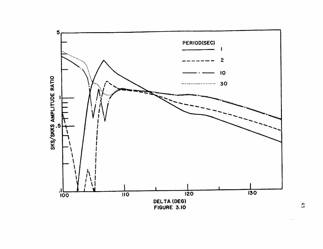
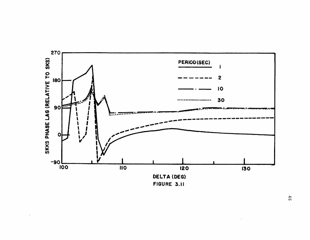
We first considered a transition zone model consisting
of a homogeneous layer of 100 kilometer thickness (model
#81 of Alexander and Phinney, 1966). Theoretical amplitude
ratio and phase lag results for this model are shown in
Figures 3.10 and 3.11. Although observed phase lag data
were only obtained from long period signals, the amplitude
ratios shown in Figure 3.5 represent data from signals
with periods ranging from 1 to 45 seconds. We find no
evidence for the large variation in amplitude ratio with
period at distances less than about 110* shown in Figure
3.10. Consequently, we next considered a model in which
the transition zone thickness was reduced to 30 kilometers
(model #94 of Alexander and Phinney, 1966). The theoretical
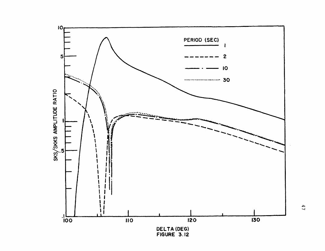
response curves for this model are shown in Figures 3.12

and 3.13. These results also exhibit a dependence on
frequency which exceeded the extent of our data scatter.
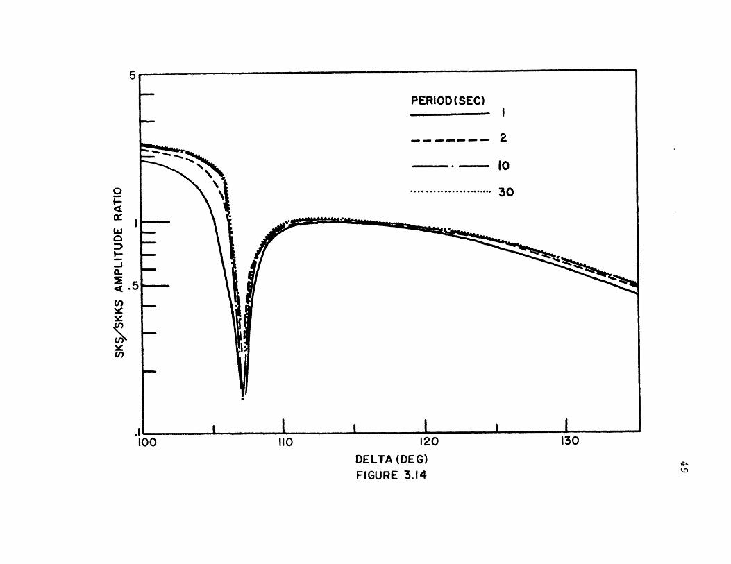
Recently, several authors (Dorman et al., 1965; Ibrahim,
1971, 1973) have proposed CMB models consisting of a number
of interbedded layers 10 to 15 kilometers thick. Figures
3.14 and 3.15 show theoretical CMB transfer function results
for the model of Dorman et al. (1965). As anticipated,
the results for this model are very similar to those for
a sharp CMB. In particular, the addition of a thin layer
transition zone does not improve the fit to our data.
3.3 Conclusions from the CMB Study
Theoretical transfer functions for layered and
non-layered CMB models have been compared to observed
SKS/SKKS amplitude ratios and SKS-SKKS phase lags. We
have isolated an SKS/SKKS amplitude ratio minimum and region
of SKS-SKKS phase shift near A = 109.50 due to the CMB
transfer function, and find that our observations can be
explained reasonably well by a non-layered interface model
similar to the B2 model of Bullen and Haddon (1967), but
with am = 13.86 km./sec. We do not purport that 13.86
km./sec. represents a derived value for the compressional wave
velocity at the CMB. Rather, we indicate that this value
for am is required to compensate for the inaccuracy of our
SKS p-A curve near '109*-110*. At present, our data does

not allow us to resolve variations in ac o c as suggested
by Balakina et al. (1966). On the other hand, we conclude
that the model of Buchbinder (1968) which incorporates a
CMB density ratio of unity does not imply transfer
functions which fit our data.
We also find that theoretical transfer functions for
models containing homogeneous transition zones 30 kilometers
or more in thickness exhibit a dependence on frequency which
exceeds the scatter of our data. However, this observation
does not preclude the existence of lateral variations in
the mantle's D" region as suggested by Alexander and
Phinney (1966), Toksoz et al. (1967), Husebye et al. (1971),
Davies and Sheppard (1972), Kanasewich et al. (1972), Vinnik
et al. (1972), Julian and Sengupta (1973) and Jordan and
Lynn (1973). Rather, it indicates that a single homogeneous
layer is an inadequate model for this region. If present,
we conclude that a CMB transition zone consists of homogeneous
layers less than about 10 to 15 kilometers in thickness. The
"sharpness" of this interface is also suggested by the
remarkable similarity of P, PcP and PKKKP for a given event-
station pair (Davies, 1971; Frasier, 1972).

TABLE 3.1
CORE - MANTLE BOUNDARY MODELS
a (km/sec) a (km/sec) p (g/sec)
TRANSITIONLAYER THICKNESS
(km)
B2 (Bullen and Haddon,1967) 13.64
8.128
Balakina et al. (1966) 13.64
8.128
Buchbinder
Dorman et al.
(1968)
(1965)
#81 (Alexander and1966)
Phinney,
13.64
7.51
13.69
13.0
11.6
10.2
8.15
13.6
13.3
8.3
#94 (Alexander and Phinney,1966)
13.6
10.0
8.3 0
5.687
9.891
1:1.818
1:1
5.65
5.66
5.67
6.2
7.304
0
7.304
0.7
7.29
7.21
6.84
6.1
5.2
0
7.5
4.8.
0
7.5
2.8
100
9.4
5.5
6.7
9.5
5.5
6.7
9.5
FIGURE CAPTIONS
Figure 3.1
Figure 3.2
Figure 3.3
Figure 3.4
Figure 3.5
Figure 3.6
Theoretical amplitude and phase curves for
CMB transmission and reflection coefficients.
Calculations were made assuming the B2 model
of Bullen and Haddon (1967).
SKS and SKKS CMB incidence angles calculated
using the B2 model of Bullen and Haddon (1967)
and the Jeffreys-Bullen Tables for SKS and
SKKS (Travis 1965).
Observed long period SKS and SKKS amplitudes
(corrected for instrument magnification, azimuth
and event magnitude as described in section 2.3).
SKS and SKKS take-off angles assuming the ray
parameters implied by equations 4.1 and 4.2 and
0 = 3.40 km./sec., 6500 = 5.28 km./sec.
SKS/SKKS amplitude ratios. Short period ratios
(solid circles) have not been corrected for
any differences in the frequency content of
SKS and SKKS.
Correlation between amplitude ratio and phase
lag data. Amplitude ratio curve (solid line)
was obtained by taking the median value of
Figure 3.5 in 1 degree intervals. Dashed curves
Figure 3.7
Figure 3.8
Figure 3.9
Figure 3.10
Figure 3.11
Figure 3.12
represent theoretical values computed for the
B2 model of Bullen and Haddon (1967), (but with
am = 13.86 km./sec.) and the SmKS ray parameters
corresponding to model SKORl.
Nomenclature for the Sagittal approximation
to curvature effect.
Theoretical SKS/SKKS amplitude ratios and SKKS
phase lags (relative to SKS) for the B2 model of
Bullen and Haddon (1967) and the Jeffreys-Bullen
travel times for SKS and SKKS (Travis 1965).
Theoretical SKS/SKKS amplitude ratios and SKKS
phase lags (relative to SKS) for the CMB models
of Balakina et al. (1966) and Buchbinder (1968).
Theoretical SKS/SKKS amplitude ratios as a
function of period for CMB model #81 of Alexander
and Phinney (1966).
Theoretical SKKS phase lags (relative to SKS)
as a function of period for CMB model #81 of
Alexander and Phinney (1966).
Theoretical SKS/SKKS amplitude ratios as a
function of period for CMB model #94 of
Alexander and Phinney (1966).

Figure 3.13
Figure 3.14
Figure 3.15
Theoretical SKKS phase lags (relative to SKS)
as a function of period for CMB model #94 of
Alexander and Phinney (1966).
Theoretical SKS/SKKS amplitude ratios as a
function of period for the CMB model of Dorman
et al. (1965).
Theoretical SKKS phase lags (relative to SKS)
as a function of period for the CMB model of
Dorman et al. (1965).

0wzuJ
-180,0 30 60
CMB INCIDENCE ANGLE (DEG)
FIGURE 3.1
90

SKS
--- SKKS
901
w
0
zw
zw
2300
120DELTA (DEG)FIGURE 3.2
ft.Nftaf-at ftft"*m tutf "fta af* No otff
01100 130
0
00 80od)c
8 ooo0- C
0 00000 o 0
0 000 000
000
Oo00
00 00000
00
06) 0
00
0
0 0
00
o0
0OCP 0
0
00
0
0
120DELTA (DEG)
I I130 100 1O1 120
DE LTA(DEG)FIGURE 3.3
SKS
07-
Coz0
LI
cc2
0
0
0o80
5-- co 0
i I
100.I
110 130
i
5 |-
00000 13>-w
s
120DELTA(DEG)FIGURE 3.4

0
wa
C,)
.5
100 110 120 130DELTA (DEG)FIGURE 3.5
0 00
0o-
I I110
gumbo*01 / I
-9o00
6 00 L - o mm .. - -
0 0 0 000 0Q *
0 0 00 0 0 0 (
A
1O1S I
120DELTA (DEG)
FIGURE 3.6
130
0o 6
0
"Jw
I-.J(L
1801
901
0H-
-90100
a I
(X-a)2 2 = R2
X2- 2X+2 2cR2
o SMALL
aze O
Xe R
2 2 2
y' =X 2 R
X 2R
/Io~Nr WAVE
SAGGITAL APPROXIMATION
FIGURE 3.7

DELTA (DEG)FIGURE 3.8
43
0
I-
w
0-
Dn
-J
360
270
CDw*m
w
0
010-

270
180
90
0
-901--100
DELTA (DEG)
110 120
DELTA (DEG)
FIGURE 3.9
BALAKINA ET AL. (1966)
-- --- BUCHBINDER (1968)
0
w
C
Cli.5
130
0
4
w0
I-:30.
4U,.
CoCoCo
DELTA (DEG)FIGURE 3.10
110 120 130DELTA (DEG)FIGURE 3.11
270
OS
90
-0
0
-90 L-100
'o --- - \WM --, O
0 N-i
I(0 1 i
000W03
DETA(DGF
cccnI
F h100 110 120 130
DELTA (DEG)FIGURE 3. 12

DELTA(DEG)FIGURE 3.13
110 120 130
DELTA (DEG)FIGURE 3.14
5
0
w
C..5
c')
100

270
DELTA (DEG)FIGURE 3.15
4. Inversion of the Outer Core Velocity Structure
This chapter delineates our preliminary model for
the outer core velocity structure which has been inverted
to fit SmKS travel time and dT/dA observations. Since
our study indicates that the true nature of the SKS
travel time curve may be more complicated than previously
thought, we have decided not to invert specific details
of the velocity structure below a radius of about 2900
kilometers until a more sophisticated inversion incor-
porating PmKP data and an analysis for uniqueness has
been completed. Instead, we present a detailed analysis
of velocities in the core's outer 600 kilometers based on
dT/dA observations and travel times corresponding to SKKS,
SKKKS, SKKKS-SKKS and SKKS-SKS. The remaining portions
of the core are constrained only by our SKKS-SKS time
differences and by the absolute times of the first SKS
arrivals. We should point out that the results presented
in this chapter are subject to any errors inherent in the
Jeffreys-Bullen ScS travel times used for "stripping"
the mantle contributions from our observations.
4.1 Constraints on the Velocity Structure for theOuter 600 Kilometers of the Core
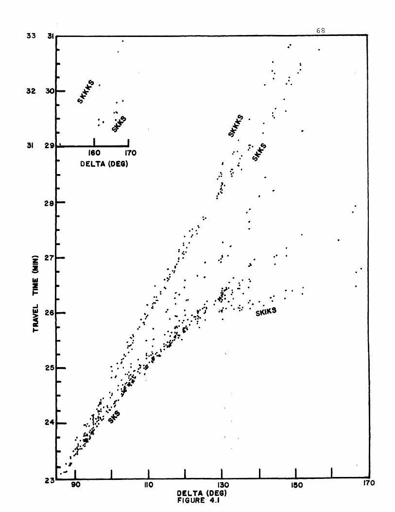
Figure 4.1 shows the total SmKS travel time
data set. Those travel times corresponding to SKKS, SKKKS
and the initial SKS onsets (usually referred to as the

AC branch) are shown in Figure 4.2. The SKS and SKKS
data from Figure 4.2 were least squares fit with a second
degree polynomial in delta and the derivative taken in
order to obtain a ray parameter versus epicentral distance
table for SKS and SKKS. These polynomials (valid for
90*<A<135*) are given in equations 4.1 and 4.2
TSKS = 1481.28 + 4.5926 (A-105') - 0.0337 (A-105') 2 4.1
TSKKS = 1523.99 + 7.0314 (A-105') - 0.0125 (A-105') 2 4.2
where the RMS deviations are 1.84 and 2.28 seconds
respectively for SKS and SKKS. We compare SKS and SKKS
travel times corresponding to equations 4.1 and 4.2 to
those of Hales and Roberts (1971) and the Jeffreys-Bullen
Tables in Table 4.1. Since we have mainly used short
period data, the fact that our travel times are generally
shorter than those of Hales and Roberts (1971) may reflect
the effect of instrument group delay.
We next "stripped" the mantle contributions from
calculated epicentral distances using the relations
presented in equations 4.3 and 4.4 and the Jeffreys-Bullen
Tables for ScS:
AK(SKS) = ASKSP - AScS(P) 4.3
AK(SKKS) = 1/ 2 [ASKKS(P) - A'O(P)] 4.4
This process provided us with ray parameter information
for core distances between 150 and 1200. Since core-
mantle boundary studies did not permit determination of
the outer core velocity at this interface, a technique
given by Randall (1970) was employed for this purpose.
This technique assumes that ( = 2danr/dknn is constant
throughout the region of interest, and that as a
consequence, velocity follows the simple power law
v = vcmb (r/r cmb) (where n = r/v and a = §. = rdv/vdr=
constant). Equations 4.5 and 4.6 (Randall, 1970) are
derived under this assumption and solved simultaneously
to provide estimates for vcmb'
tK = 2rcmb/(l-a)vcmb sin[AK(l-a)/2] 4.5
p = dtK/dAK = OTrcmb/l80 vcmb) cos [AK(1-)/2 4.6
This approach was applied to SKKS(90*-130*) and SKS(90*)
data on p, tK and AK. Values for vcmb obtained by this
method (assuming rcmb = 3485 kilometers) were grouped
between 8.006 and 8.011 km./sec. using data from SKKS

(90*-100*), but then increased steadily as the ray
bottoming depth increased. We show this trend in the
results of Table 4.2.
The values of v b which we have obtained are
slightly higher than the values of 7.893 to 7.909 km./sec.
obtained by Hales and Roberts (1971), but in good agreement
with the recently derived velocities of 8.02 km./sec.
(Jordan, 1973), 8.05 km./sec. (Toksoz et al., 1973) and
8.056 km./sec. (Qamar, 1973). It is important to note
that similar to our results, Randall (1970) obtained a
relatively high value for vcmb (8.256 km./sec.) using
SKS data. This observation suggests that the simple
velocity power law assumption may only be valid in the
outer few hundred kilbmeters of the core.
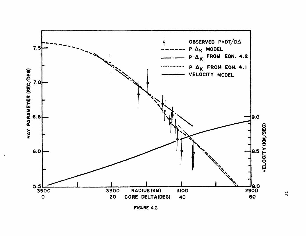
The p-AK curves obtained from equations 4.1 and 4.2
are compared to observed SKKS dT/dA values from LASA
and NORSAR in Figure 4.3. This diagram indicates that
the p-AK curve relevant to the determination of compressional
wave velocities in the upper 600 kilometers of the core
possesses structure not contained in the limited information
provided by travel times alone. In particular, our
observations indicate the existence of a significant
increase in the slope of the p-A K curve between core
distances of about 350 to 40*. This region of increased
p-AK slopes corresponds to SKKS arrivals between epicentral
55
distances of about 1100 to 120*. Since the geometrical
spreading effect is proportional to Id 2T/dA 21 (Bullen, 1965),
we anticipate that this slope change should be reflected in
our amplitude data. Figure 3.3 shows that this is indeed
the case. SKKS amplitudes increase rapidly with increasing
epicentral distance, reach a maximum between distances of
about 110* and 1200 and then decrease. We conclude that
this rapid slope increase in the p-AK curve is responsible
for the amplitude ratio minimum in region C of Figure 3.6.
Although this feature is localized between distances of
about 116* to 1200 in Figure 3.6, we believe that region C
encompasses the approximate distance range 112 0<A<120*
(the minimum being located near 117.50), but that SKS
focusing (discussed in section 4.3) is superimposed on this
feature in region B (112*<A<115*). As an independent check,
we examined SKKKS/SKKS amplitude ratios. Preliminary
results from this study shown in Figure 4.4 indicate that
the SKKKS/SKKS amplitude ratio gradually increases with
increasing delta until it reaches a maximum at distances
of about 1500 to 165*. This maximum location is consistent
with the results for SKKS.
Using 8.01 km./sec. as a starting value for vcmb' we
next examined a suite of p-AK models in order to determine
which ones would simultaneously fit our dT/dA data and
produce velocity structures consistent with observed
travel times. We found that the p-AK curve shown in
Figure 4.3 provided the best fit to both sets of data.
The resulting velocity structure (shown in Figure 4.3) is
characterized by a CMB velocity of 8.015 km./sec. and a
change in dv/dr from about -0.00155 sec~ for the outer
250 kilometers to a maximum of about -0.0022 sec near
a radius of 3175 kilometers. These results are consistent
with those from the vcmb extrapolation, and the break
down of the Randall technique for rays which bottom more
than a few hundred kilometers below the CMB. We should
point out that p-AK models which provided a better fit
to observed SKKS ray parameters less than about 6.2 sec./
deg..produced core velocities too high to satisfy our
travel time data for SKS and SKKS (A>l250 ).
Although a detailed analysis similar to the study
by Wiggins et al. (1973) should be made, a preliminary
study indicates that the scatter in our SKS, SKKS, SKKKS,
SKKKS-SKKS and SKKS-SKS times constrain the model of
Figure 4.3 within about ±0.02 km./sec (subject to
uncertainties in the Jeffreys-Bullen ScS times). We
discuss the fit to these travel times in section 4.2.
4.2 Analysis of Core Model SKORl
Having obtained a velocity model for the outer
600 kilometers of the core, we combined our p-AK data from
section 4.1 with the SKS ray parameter data implied by

57
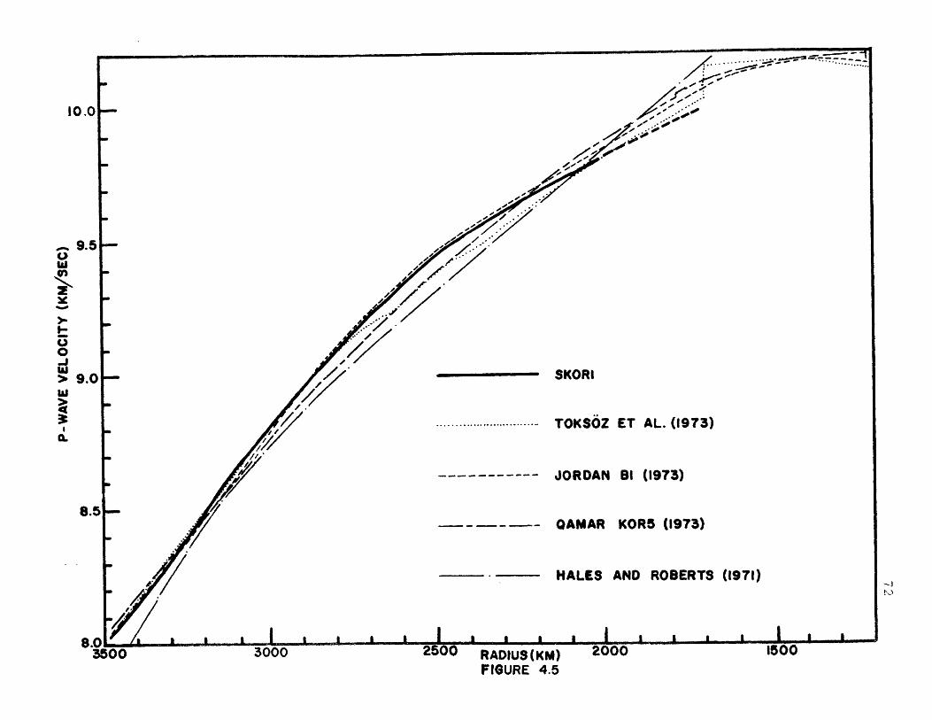
equation 4.1. The resulting p-AK curve was inverted
using the Herglotz-Wiechert technique to obtain our base
model for the outer core velocity structure. This velocity
model (SKORl) is compared to other core models in Figure
4.5 and listed in Table 4.3. Except for the change in
dv/dr between radii of 3050 and 3250 kilometers derived
in section 4.1, SKOR1 is similar to most of the other
recently derived core models (particularly the Bl model
of Jordan, 1973). As we discuss in section 4.3, however,
SKORI may require revision at radii less than about 2700
kilometers in order to satisfy our total SKS data set.
We first considered the fit of SKORl to our absolute
travel times. Figure 4.2 shows the comparison between
theoretical SKS, SKKS and SKKKS travel times computed for
SKORl and those observed in this study. The theoretical
travel times shown in this diagram all fall within the
limits of our data scatter, with SKS showing a slight
tendency to be earlier than our observed times at distances
qreater than about 100* (bottoming radius less than about
2700 kilometers). Next, we compared theoretical SKKKS-SKKS
and SKKS-SKS time differences computed for SKOR1 to our
observed data. Figure 4.6 shows that these theoretical
time differences fall within the scatter of our data as
in the case of the absolute travel times.
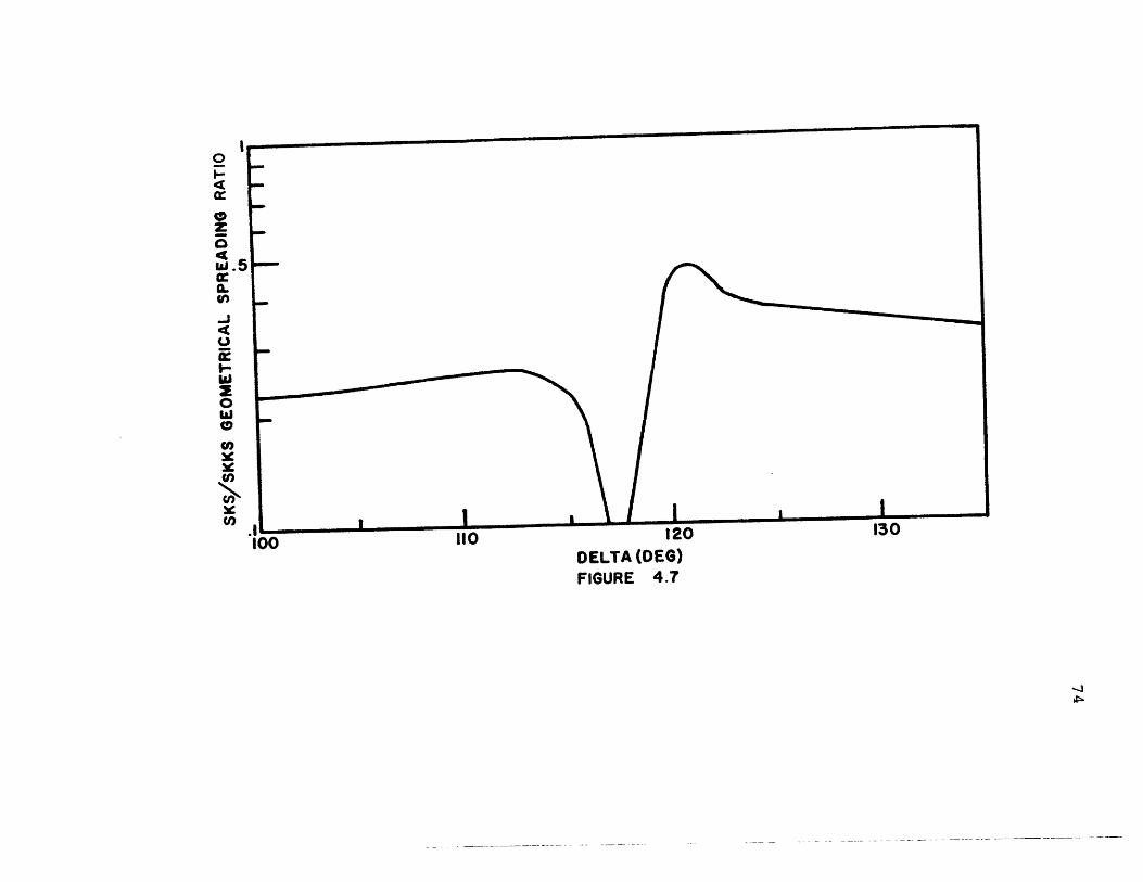
Figure 4.7 shows the smoothed SKS/SKKS geometrical

58
spreading ratio computed for SKORl. We find that SKOR1
reproduces the amplitude ratio minimum at distances of
about 117.5*. It should also be noted that the decrease
in slope of our p-AK curve between 37 *%AK%4 2* produces
a region of high SKS/SKKS amplitude ratios between
120*%A%123* similar to our observations in region D of
Figure 3.6. Computed slopes of kn(ASKS/ASKKS) versus
frequency plots are shown in Figure 4.8. This diagram
indicates that the effect of attenuation may differ for
SKS and SKKS. Consequently, differences in SKS and SKKS
attenuation, and possibly tunnelling effects (Richards,
1973) will have to be considered before theoretical amp-
litude ratios such as those given in Figure 4.7 can be
placed in proper perspective to observed ratios.
As an independent check, we computed theoretical PKP
travel times for model SKOR1 and the mantle P wave
velocities from the Bl model of Jordan (1973). These
theoretical travel times are compared to the PKP times
of Perrin (1968) in Table 4.4. We find that theoretical
and observed PKPAB times agree within 0.5 seconds for
opicentral distances of 170* to 1500 (bottoming radius
greater than about 2250 kilometers), but that our times
are increasingly too long for rays bottoming below this
radius. We also find that our PKP focus location of
145.6* is slightly larger than the value of 144.24

determined by Shahidi (1968). However, we do not
purport to have constrained velocities in the lower
portions of the outer core at this time.
4.3 Evidence for Additional SKS Travel Time Branches
The data presented in this section represent
preliminary observations indicative of additional SKS
travel time branches. As such, they are presented at
this time in order to provide insight into areas
requiring future study.
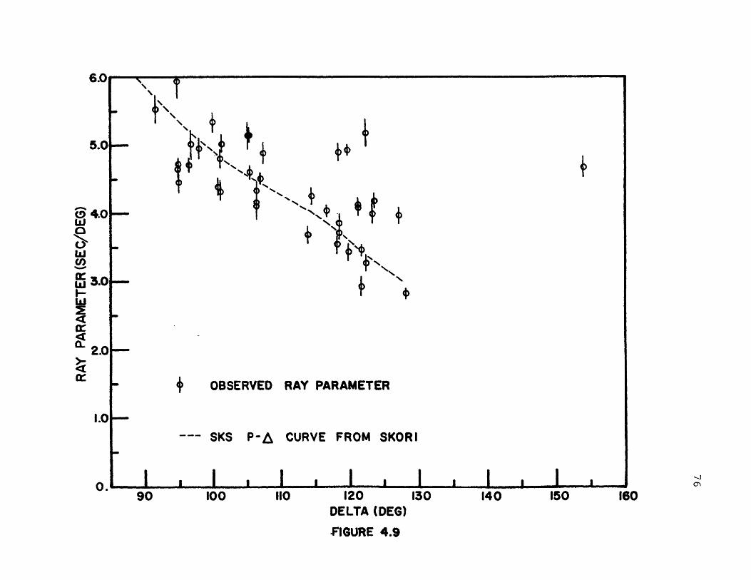
Figure 4.9 shows a comparison'between the p-A
curve implied by SKOR1 and our observed SKS ray
parameters. The data shown in this diagram indicates
that the SKS travel time curve may possess "secondary"
branches in addition to the AC-branch. Figure 4.1 shows
an alignment of arrivals between SKS and SKKS. Similar
observations were made by Gutenberg and Richter (1936).
These travel times may correlate with our dT/dA observations
between 5.0 and 5.5 sec./deg. Figure 4.10 shows a detailed
section of our travel time data for 85*<A<105*. It is
important to note that the triangles shown in this
diagram represent travel times for arrivals observed after
the initial SKS onset for a given seismogram. This diagram
shows that secondary SKS arrivals form a cusp at distances
of about 92*.

Figure 4.11 shows a detailed section of our data at
distances where other "secondary" SKS arrivals have been
observed. This diagram illustrates one alignment of
arrivals which have a slope of about 4.0 sec./deg. These
data may correlate with the p-A structure observed at this
value of wave slowness in Figure 4.9. Figures 3.1 and 3.6
illustrate the presence of high SKS amplitudes and SKS-SKKS
phase shifts indicative of SKS focusing between distances of
1120 and 1150. The dT/dA observations near 4.0 sec./deg.
shown in Figure 4.9 suggest that this focusing may be
associated with the cusp of the proposed SKS branch.
Figure 4.11 also shows an alignment of arrivals
with a slope of about 3.1 sec./deg. These data may be
the SKS equivalent of the precursors to PKP. Figure 4.2
shows several examples of the observed "secondary" SKS
arrivals.
4.4 Conclusions From The Outer Core Velocity Study
We have obtained a preliminary model for the
outer core velocity structure based on absolute and
differential SmKS travel times. The main emphasis of
this study was that of constraining the outer 600 kilometers
of the core. We found that compressional wave velocities
start from a value of about 8.015 km/sec. at the CMB and
increase with a nearly constant rate in the outer 250
kilometers of the core. The rate of velocity increase
with increasing depth is significantly higher between
radii of about 3250 and 3050 kilometers, however.
We inverted an outer core velocity model (SKORl)
by using our results for the outer 600 kilometers and
constraining the remaining depths with our travel times
for initial SKS onsets. SKOR1 possesses a positive
perturbation in compressional wave velocity (relative
to other recent core models) centered at a radius of
about 2500 kilometers. This feature is very similar to
the results given in the Bl model of Jordan (1973).
Section 4.3 of this chapter provided initial evidence
which indicates the existence of additional SKS travel
time branches. We are currently examining a combined
PmKP and SmKS data set in an effort to arrive at a
consistent explanation for these "secondary" arrivals.

TABLE 4.1
COMPARISON OF SKS AND SKKS TRAVEL
(DEPTH OF FOCUS = 33 KM)
DISTANCE
900
950
1000
1050
1100
1150
1200
1250
1300
EQUATION 4.1
1404.8
1432.0
1457.5
1481.3
1503.4
1523.8
1542.6
1559.6
1575.0
SKS
HALES AND ROBERTS
1405.8
1434.4
1460.7
1484.9
1506.8
1526.5
1544.0
1559.4
1572.5
J-B
1403.7
1432.0
1457.9
1481.4
1503.1
1522.8
1540.8
1556.7
1570.7
SKKS
EQUATION 4.2 HALES AND ROBERTS J-B
1415.7
1452.4
1488.5
1524.0
1558.8
1593.1
1626.7
1659.6
1692.0
1421.3
1458.4
1494.7
1530.2
1564.9
1598.8
1631.9
1664.0
1695.5
1413.0
1449.0
1485.0
1521.0
1556.0
1591.0
1625.0
1657.9
1690.9
TIMES

TABLE 4.2
RESULTS FROM VCMB EXTRAPOLATION
p (sec/deg)
7.4064
7.1564
6.9064
6.6564
6.4064
5.6392
t (sec) r( mi C km/sec)k (sc bottomning CMB
113.167
165.315
213.497
258.567
300.990
364.053
3435
3380
3310
3180
3020
2890
8.011
8.006
8.029
8.063
8.104
8.173
SOURCE
SKKS
SKKS
SKKS
SKKS
SKKS
SKS
(900)
(1000)
(1100)
(1200)
(1300)
(900)
Ak (DEG)
15.028
22.191
29.043
35.688
42.183
53.298
-0.6913
-0.7680
-0.6706
-0.5728
-0.4888
-0.5285
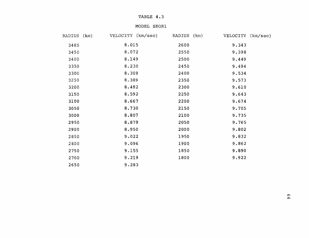
TABLE 4.3
MODEL SKOR1
RADIUS (km)
3485
3450
3400
3350
3300
3250
3200
3150
3100
3050
3000
2950
2900
2850
2800
2750
2700
2650
VELOCITY (km/sec)
8.015
8.072
8.149
8.230
8.308
8.389
8.482
8.592
8.667
8.730
8.807
8.879
8.950
9.022
9.096
9.155
9.219
9.283
RADIUS (km)
2600
2550
2500
2450
2400
2350
2300
2250
2200
2150
2100
2050
2000
1950
1900
1850
1800
VELOCITY
9.343
9.398
9.449
9.494
9.534
9.573
9.610
9.643
9.674
9.705
9.735
9.765
9.802
9.832
9.862
9.890
9.922
(km/sec)
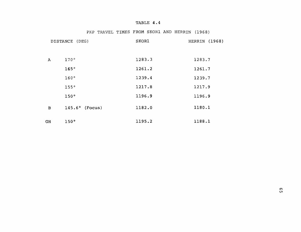
TABLE 4.4
PKP TRAVEL TIMES FROM SKORl AND HERRIN (1968)
DISTANCE (DEG)
A 1700
1650
1600
1550
1500
B 145.6* (Focus)
SKOR1
1283.3
1261.2
1239.4
1217.8
1196.9
1182.0
1195.2
HERRIN (1968)
1283.7
1261.7
1239.7
1217.9
1196.9
1180.1
GH 1500 1188.1
66
FIGURE CAPTIONS
Figure 4.1
Figure 4.2
Figure 4.3
Figure 4.4
Figure 4.5
Figure 4.6
Figure 4.7
Figure 4.8
Observed SKS, SKKS and SKKKS Travel Times
Travel times for SKKS, SKKKS and first arrivals
of SKS. Fit of theoretical travel times for
SKOR1 to these data.
Observed SKKS dT/dA values and p-Ak curve for
outer 600 kilometers of core. Bars on ray
parameters indicate 95% confidence limits.
Diagram also shows inverted velocity structure
for outer 600 kilometers of core.
Observed SKKKS/SKKS amplitude ratios.
Comparison of velocity model SKOR1 to other
recently published models (Hales and Roberts,
1971; Toksoz et al., 1973; Jordan, 1973;
Qamar, 1973).
Fit of theoretical SKKKS-SKKS and SKKS-SKS
time differences computed for SKORl to
observed data from this study.
Theoretical SKS/SKKS geometrical spreading
ratios (smoothed) computed for core model
SKORl.
Observed slopes from plots of kn (ASKS/ASKKS
versus frequency.
Figure 4.9
Figure 4.10
Figure 4. 11
Comparison between observed SKS dT/dA values
and the SKS p-A curve calculated for core
model SKORl. Bars on ray parameters indicate
95% confidence limits.
Detailed section of observed travel times
at distances between 85* and 105*. Triangles
indicate travel times for onsets observed
after the first SKS arrival on a given seismo-
gram.
Detailed section of observed travel times
showing "secondary" SKS arrivals. Triangles
indicate travel times for onsets observed
after the first SKS arrival on a given
seismogram. Dashed lines indicate a preliminary
interpretation of these "secondary" arrivals.
COj
29 *L -J
* DELTA (DES)
0 %
: ~.*00
0.
0,*09
0 *
0 * 00000 0
o 5
00: ~~ 2~.:* ~
- , - - '
o 40
004 0 0
130DELTA (DES)FIGURE 4.1
33 31
301-32
31160 170
Co4**0~
*0
CO
27-
.00
08. .
261--
* 0
*'*
25.0
01 -
246...
-- ___MEMNON23 90 150 170
2 9 --
* -.

I150
DELTA (DEe)
4~)
/
.9/
/ o,1//
//
/ 0~
9*/ 9/
//
*0/
/
/ 8
zip,49/
33
32
/* 43 0
// J
0~
/ ,99
/. /
-'* ?'*
:,
29 25
- ',' /// 9.
/0/.1 /"p /
/km.... 9'.
/
/'I
9..
24 9/I
I. /V,e ~A
/9 V
/999 */9
I */Ii
'
/4/
90
9/
9'.0*
/I.
I 9g..
/)91~
/
I100
- OBSERVED TRAVEL TIMES
TRAVEL TIMES COMPUTED FOR
110DELTA (DEG)FIGURE 4.2
I..... 140
//
9/ 9/
/ / // / *..
/ /* 9 / 9//
/*
1%,9/ /
160 170
4-7
-
/
/
31 27-- / .1**'1
/ *~,9
I, .~/
!30;/
//
I* 1
0*~'
a-
I':4.
SKORI
130120
//
//
-I
C
2
VELOCITY MODEL7.o-
w NS9.0~6.5--9.
4r0
6.0 8.5
Olts 0* w
3500 3300 RADIUS (KM) 3100 29000 20 CORE DELTA(DEG) 40 60
FIGURE 4.3

F'
000
0
o SKKKS/SKKS
I I I130
FROM OUR DATA
SSKKKS/SKKS FROM DA TA OFHALES AND ROBERTS (1971)
II150 170
DELTA (DEG)
FIGURE 4.4
0
I4
w0I--i
(I)
cl)
c,)
c,,
110 I I
I
SKORI
TOKSOZ ET AL. (1973)
JORDAN 81 (1973)
QAMAR KORS (1973)
HALES AND ROBERTS (1971)
RADIUS (KM)FIGURE 4.5
10.01
9.5
9.0
wU)
I
U0-Iww4
0.

150
85 95110
hd ICAL TIME DIFFERENCESICAL TIME DIFFERENCESRE MODEL SKORI
D TIME DIFFERENCES0~*
--- THEORET
FROM CO
* OBSERVE
mm
---
0 *M
0-of
* S ~ -5.
-- 5---
I e~1.1;1
wIO
w
wu.50U.
- 0*
105120
I 1
115 125130 140
DELTA (DEG)
FIGURE 4.6
135150
*~
S*0
S----
-
~0*
-5--5-5-
5-5-5-
160 170
a I
--..
- 00A0
SK
S/S
KK
S
GE
OM
ETR
ICA
L SP
REA
DIN
G
RAT
IO
'10
I~j
m
I
0~
TII

SLO
PE
OF
[LN
(ASK
S/A
SKK
S)
(T1 to O
VS.
FR
EQU
ENC
Y]
6.O x m
5.0--
OBSERVED
1.01----- SKS P-A
a I I 1
RAY PARAMETER
CURVE FROM SKORI
I 1 a I120
DELTA (DEG)
FIGURE 4.9
4.0Qc-)w
I
3.01-
2.0
90 100 110I I
130a 1
140 150 I60a I a I A I I I

//
251--
o/0
/
/
/0'
0/
/A
/ *
//$
og/0//
/
90
/470
9595
DELTA (DEG)
FIGURE 4.10
J
4
'A
240-
23
85 100 105

TRA
VE
L TI
ME
(MIN
)
N
-- 0%0
%1
oto.
O%
%0
%,
0%
000
-co
o 3
\
(00
r 1,
0
0
i m
m
w c
.00
Z
'-
WI
o 0
0
CO m
0
24
0
r z
O0
0 4M
References
Adams, R.D. and M.J. Randall, The fine structure of
the earth's core, Bull. Seism. Soc. Am., 54,
1299-1313, 1964.
Adams, R.D., Multiple inner core reflections from a
Novaya Zemlya explosion, Bull. Seism. Soc. Am.
62, 1063-1071, 1972.
Alexander, S.S. and R.A. Phinney, A study of the core-
mantle boundary using P waves diffracted by the
earth's core, J. Geophys. Res., 71, 5943-5958, 1966.
Anderson, D.L. and T.H. Jordan, The structure, composition
and evolution of the earth's interior, Trans. Am.
Geophys. Union (EOS), 53, 451, 1972.
Balakina, L.M., A.V. Vvedenskaya, Yu A. Kolesnikow,
Study of the boundary of the earth's core from
spectral analysis of seismic waves, Phys. Solid
Earth, 8, 492-499, 1966.
Berzon, I.S. and I.P. Pasechnik, Dynamic characteristics
of the PcP wave in a thin-layer model of the
transition region between the mantle and the core,
Phys. Solid Earth, 6, 350-357, 1972.
Bolt, B.A., The velocity of seismic waves near the
earth's center, Bull. Seism. Soc. Am., 54, 191-
208, 1964.
Bolt, B.A., PdP and PKiKP waves and diffracted PcP
waves, Geophys. J. R. Astr. Soc., 20, 367-382, 1970.
Bolt, B.A. and A. Qamar, Upper bound to the density
jump at the boundary of the earth's inner core,
Nature, 228, 148-150, 1970.
Bolt, B.A., The density distribution near the base of
the mantle and near the earth's center, Phys. Earth
Planet. Interiors, 5, 301-311, 1972.
Born, M. and E. Wolf, ,Principles of Optics, MacMillan,
New York, 1964.
Buchbinder, G.G.R., Properties of the core-mantle
boundary and observations of PcP, J. Geophys. Res.
73, 5901-5923, 1968.
Buchbinder, G.G.R., A velocity structure of the earth's
core, Bull. Seism. Soc. Am., 61, 429-456, 1971.
Bullen, K.E., Ellipticity connections to waves through
the earth's central core, M.N.R.A.S., Geophys., Suppl.
4, 317-331, 1939.
Bullen, K.E., An introduction to the theory of seismolo
Cambridge University Press, England, 381 p., 1965.
Bullen, K.E. and R.A.W. Haddon, Earth models based on
compressibility theory, Phys. Earth Planet. Interiors,
1, 1-13, 1967.
Chowdhury, D.K. and C.W. Frasier, Observations of PcP
and P phases at LASA at distances from 260 to 400 ,

J. Geophys. Res., 78, 6021-6027, 1973.
Cleary, J., The S velocity at the core-mantle boundary,
from observations of diffracted S, Bull. Seism. Soc.
Am., 59, 1399-1405, 1969.
Davies, D., Source function for explosions from core
reflections, Seismic Discrimination Semiannual
Technical Report to the Advanced Research Projects
Agency, Lincoln Laboratory, M.I.T., (31 Dec. 1970),
3-4.
Davies, D., and R.M. Sheppard, Lateral heterogeneity in
the earth's mantle, Nature, 239, 318-323, 1972.
Derr, J.S., Internal structure of the earth inferred
from free oscillations, J. Geophys. Res, 74,
5202-5219, 1969.
Dorman, J., J. Ewing and L.E. Alsop, Oscillations of
the earth: New core-mantle boundary model based on
low-order free vibrations, Proc. Natl. Acad. Sci.,
54, 364-368, 1965.
Engdahl, E.R., Core phases and the earth's core, Ph.D.
Thesis, St. Louis University, St. Louis, Missouri,
197 p., 1968.
Engdahl, E.R., E.A. Flinn, and C.F. Romney, Seismic
waves reflected from the earth's inner core, Nature,
228, 852-853, 1970.

82
Ergin, K., Seismic evidence for a new layered structure
of the earth's core, J. Geophys. Res., 72, 3669-3687,
1967.
Frasier, C.W., Amplitudes of P and PcP phases at LASA,
Trans. Am. Geophys. Union (EOS), 53, 600, 1972.
Gilbert, J.F. and G.E. Backus, Propagator matrices in
elastic wave and vibration problems, Geophysics
31, 326-332, 1966.
Gutenberg, B. and C.F. Richter, On seismic waves,
Gerl. Beitr. Geophys., 43, 56-133, 1934.
Gutenberg, B. and C.F. Richter, On seismic waves, second
paper, Gerl. Beitr. Geophys., 45, 280-360, 1935.
Gutenberg, B. and C.F. Richter, On seismic waves, third
paper, Gerl. Beitr. Geophys., 47, 73-131, 1936.
Gutenberg, B., Wave velocities in the earth's core,
Bull. Seism. Soc. Am., 48, 301-314, 1958.
Hales, A.L. and J.L. Roberts, The travel times of S and
SKS, Bull. Seism. Soc. Am., 60, 461-489, 1970.
Hales, A.L. and J.L. Poberts, The velocity distribution
in the core, Trans. Am. Geophys. Union (EOS),
52, 283, 1971a.
Hales, A.L. and J.L. Roberts, The velocities in the outer
core, Bull. Seism. Soc. Am., 61, 1051-1059, 1971b.
Haskell, N.A., The dispersion of surface waves on
multilayered media, Bull. Seism. Soc. Am., 43,
17-34, 1953.
Haskell, N.A., Crustal reflection of plane P and SV
waves, J. Geophys. Res., 67, 4751-4767, 1962.
Herrin, E., 1968 seismological tables for P phases,
Bull. Seism. Soc. Am., 58, 1193-1241, 1968.
Husebye, E.S., R. Kanestrom, and R. Rud, Observations
of vertical and lateral P-velocity anomalies in the
earth's mantle using the Fennoscandian Continental
Array, Geophys.J.R. Astr. Soc., 25, 3-16, 1971.
Ibrahim, Abou-Bakr K., The amplitude ratio PcP/P and
the core-mantle boundary, Pure and Appl. Geophys.
91, 114-133, 1971.
Ibrahim, Abou-Bakr K., Evidences for a low-velocity
core-mantle transition zone, Phys. Earth Planet.
Interiors, 7, 187-198, 1973.
Jeffreys, H., Southern earthquakes and the core waves,
M.N.R.A.S., Geophys. Suppl., 4, 281, 1938.
Jeffreys, H., The times of the core waves, M.N.R.A.S.,
Geophys. Suppl., 4, 548-561, 1939a.
Jeffreys, H., The times of the core waves (second paper),
M.N.R.A.S., Geophys. Suppl., 4, 594-615, 1939b.
Jeffreys, H. and E.R. Lapwood, The reflection of a pulse
within a sphere, Proc. Roy. Soc. (London) A, 241,
455-479, 1957.
Jordan, T.H., Estimation of the radial variation of
seismic velocities and density in the earth, Ph.D.
Thesis, California Institute of Technology,
Pasadena, California, 199 p., 1973.
Jordan, T.H. and W.S. Lynn, Lateral heterogeneity of the
lower mantle from the observations of ScS-S
differential travel times, Trans. Am. Geophys.
Union, (EOS), 54, 363, 1973.
Julian, B.R., D. Davies, and R.M. Sheppard, PKJKP,
Nature, 235, 317-318, 1972.
Julian, B.R. and Mrinal K. Sengupta, Seismic travel
time evidence for lateral inhomogeneity in the
deep mantle, in press, Nature, 1973.
Kanamori, H., Spectrum of P and PcP in relation to
the mantle-core boundary and attenuation in the
mantle, J. Geophys. Res., 72, 559-571, 1967.
Kanasewich, E.R., R.M. Ellis, C.H. Chapman, and
P.R. Gutowski, Teleseismic array evidence for
inhomogeneities in the lower mantle and the origin
of the Hawaiian Islands, Nature Physical Science,
239, 99-100, 1972.
Kelley, E.J., Limited network processing of seismic signals;
Lincoln Laboratory Group Report 1964-44, 1964
Kogan, S.D., A study of the dynamics of a longitudinal
wave reflected from the earth's core, Phys. Solid

Earth, 6, 339-349, 1972.
Qamar, A., Revised velocities in the earth's core,
Bull. Seism. Soc. Am., 63, 1073-1105, 1973.
Randall, M.J., SKS and seismic velocities in the outer
core, Geophys. J.R. Astr. Soc., 21, 441-445, 1970.
Richards, P.G., Calculation of body waves, for caustics
and tunnelling in core phases, in press, 1973.
Sacks, S., Diffracted wave studies of the earth's core,
1, amplitude, core size, and rigidity, J. Geophys.
Res., 71, 1173-1181, 1966.
Sacks, S., Diffracted P-wave studies of the earth's
core, 2, lower mantle velocity, core size, lower
mantle structure, J. Geophys. Res., 72, 2589-2594, 1967.
Shahidi, M., Variation of amplitude of PKP across the
caustic, Phys. Earth Planet. Interiors, 1, 97-102,
1968.
Shimamura, H. and R. Sato, Model experiments on body
waves - travel times, amplitudes, wave forms and
attenuation, J. Phys. Earth, 13, 10-33, 1965.
Shurbet, D.H., The earthquake P phases which penetrate
the earth's core, Bull. Seism. Soc. Am., 57,
875-890, 1967.
Thomson, W.T., Transmission of elastic waves through
a stratified solid medium, J. Appl. Phys., 21,
89-93, 1950.

Toksoz, M.N., M.A. Chinnery, and D.L. Anderson,
Inhomogeneities in the earth's mantle, Geophys.
J.R. Astr. Soc., 13, 31-59, 1967.
Toksoz, M.N., E.S. Husebye and R.A. Wiggins, Structure
of the earth's core, in preparation, 1973.
Travis, H.S., Interpolated Jeffreys and Bullen
Seismological Tables, Tech Report No. 65-35, The
Geotechnical Corp., Garland, Texas, 162 p., 1965.
Vinnik, L.P. and G.G. Dashkov, PcP waves from atomic
explosions and the nature of the core-mantle
boundary, Phys. Solid Earth, 1, 4-9, 1970.
Vinnik, L.P., A.A. Lukk, and A.V. Nikolaev, Inhomogeneities
in the lower mantle, Phys. Earth Planet. Interiors,
5, 328-331, 1972.
Wiggins, R.A., G.A. McMechan and M.N. Toksbz, Range of
earth structure nonuniqueness implied by body wave
observations, Rev. Geophys. Space Phys., 11
87-113, 1973.
Yanovskaya, T.B., Determination of a set of velocity-depth
curves for the transition zone of the earth's core
from travel times of successive arrivals of PKP
waves, Geophys. J. R. Astr. Soc., 29, 227-235, 1972.
Appendix. Reflection and Transmission Coefficients
The nomenclature used in the following derivation of
the CMB reflection and transmission response is provided in
Figure Al and Table Al. Coefficients pertinent to our dis-
cussion of SKS and-SKKS arrivals include:
1) P-P reflection coefficient for a fluid-solid interface
R Anpp Ann
2) P-S transmission coefficient for a fluid-solid interface
T psn
3) S-P transmission coefficient for a solid-fluid interface
A'nsp
Al The P-P Reflection Coefficient
Transverse wave potentials vanish in the fluid half space.
In addition, there will be no potentials corresponding to
incident longitudinal and transverse waves in the solid half
space. Consequently,
1 1 n n
Using the notation of Haskell (1953), and letting
A = an-1 - an-2 . . a2 we have:
un-1/c
wn-l /c
u /c
w /c
Since T _-l= 0 and un-1 does not have to
Al.1
be continuous
(because the nth layer is fluid), we have the following
relationship:
u n1
wn-1E
n
A ' + An n
n n
0
0
Al.2
But now E must be appropriately modified to account for then
fluid nature of the n th layer. First consider the equations
for wn-1/c and an-1
20 na/c) r n0 n /)an
Pn an 2(n-1)
2-(a /c)r (A ' - A ')
n /) an n n
nan2 n-1A n + A nAl.3
rn-l
0
Tn- 1
A '+ A ''
In n
0 A ' - 'ILn n

We next note that Yn = 0 (since Y= 2(P/c) 2). Therefore,
an an n n
p na:2 (A n' + A '') 3Al.4
According to equation 2.12 of Haskell (1953), we have the
following:
= E2
A 2 2+ A 2
2 2
2 2
+ W2
Al.5
However, u, w, a, and T are continuous from layer 1 to
layer 2. Figure A2 and the definitions of the D and E matrices
given in Haskell (1953) show us that
E = Lim D1 d-+0 1
Consequently,
A2'+ A 21
A2 2
W2 ~W 2
o2+ w2
= E
I'I
I I
I,1
(A)1 1
Al.6
u 1 /c
G 1
W 2'
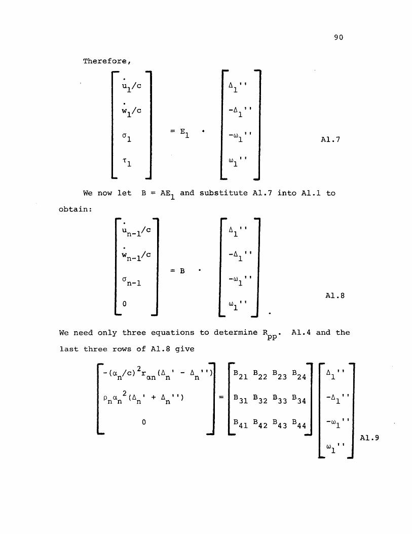
Therefore,
u/c
w1/c
We now let
= E
B = AE 1
Al ,
-A
_1
mW 1 '
and substitute Al.7 into Al.1 to
obtain:
un-l/c
wn-l /c
a n-1
0J
-A W
-W ''~1
oW ' '
We need only three equations to determine Rpp
Al.4 and
last three rows of Al.8 give
-(an /c)n -n (A
pna n (A
- '')n
'')
B B B B21 22 23 24
B31 B32 B33 B34
Bg B4 B43B41 B42 B43 B 44
Al.7
Al .8
the
-A1lI
-o
Al.9I
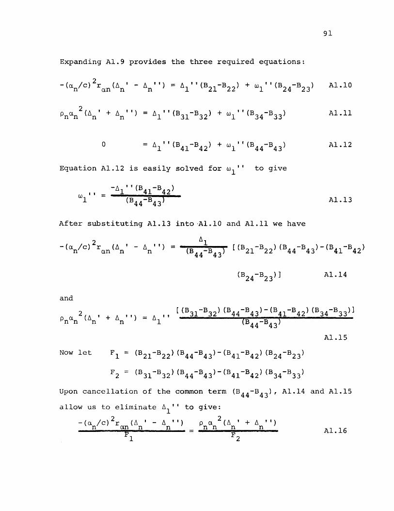
91
Expanding Al.9 provides the three required equations:
-(an/c) 2r an n
pnan2 n n
- A n') = A 1 ''(B 2 1 -B 2 2 )
A1' '(B31-B32)
A ' ''(B 4-B 42 )
+ W1 ''(B24-B23)
+ o I'' (B 3 4 -B 3 3 )
+ W 1 ' (B 44
Equation Al.12
l
is easily solved for
1 '_'_(B 4 1 -B 4 2
(B 4 4 -B 4
After substituting Al.13
-(a n/c) 2an n
into -Al.10
A
n (B -B )
and Al.ll we have
[(B2 1 -B 2 2 ) (B 4 4 -B4 3 )-(B 4 1 -B 4 2 )
(B 2 4 -B 2 3 ) ]
2 ,pnan (n' + An A1
,t [(B 31-B32) (B 4 4 -B4 3 )-(B 4 1 -B 4 2) (B3 4 -B 3 3]
(B 4 4 -B 4 3 )
F1 = (B 2 1 -B 2 2 ) (B 4 4 -B 4 3 )-(B 4 1 -B 4 2 ) (B 2 4 -B 2 3)
F 2 = (B 3 1 -B 3 2 )(B 4 4 -B 4 3 )-(B 4 1 -B 4 2 )(B 3 4 -B 3 3 )
Upon cancellation of the common term (B -B ) ,
allow us to eliminate A '' to give:
A1.14 and Al.15
-(a /c)2 r (Anan nF,
n Pna n(An + A '')Al.16
F 2
Al.10
Al.11
-B 4 3 ) Al.12
' Ito give
Al.13
and
Al.14
Now let
Al. 15
W 1

-I
Consequently,
A ' I[F2 n 2ran-F p nan2 = A n'[F2 (n/c)2 r an+F p nLn2
Al.17
The desired reflection coefficient is obtained after cancelling
A,R = n
n
ra
-F p + F2
c
Fyp + F2ra1pn 2 2
C
A2 The P-S Transmission Coefficient
The boundary conditions on the potentials for this case
are identical to those for the previous reflection coefficient.
Equation Al.12 implies the following identity:
A = - (B 44-B 43)(B41-B 42)
Equation A2.1 is next substituted into Al.10 and Al.ll to give
A2.1
-(an/c) r an (An -An 1
(B2 4-B23) (B 41-B42 )-(B 44 -B4 3) (B21-B22)
(B4 1- 42 )
-F 1 '
(B 4 1 -B 4 2 )
2pna~n (n I+n l
A2.2
B -B41 42
A2.341 ~42
2
n
Al.18
And
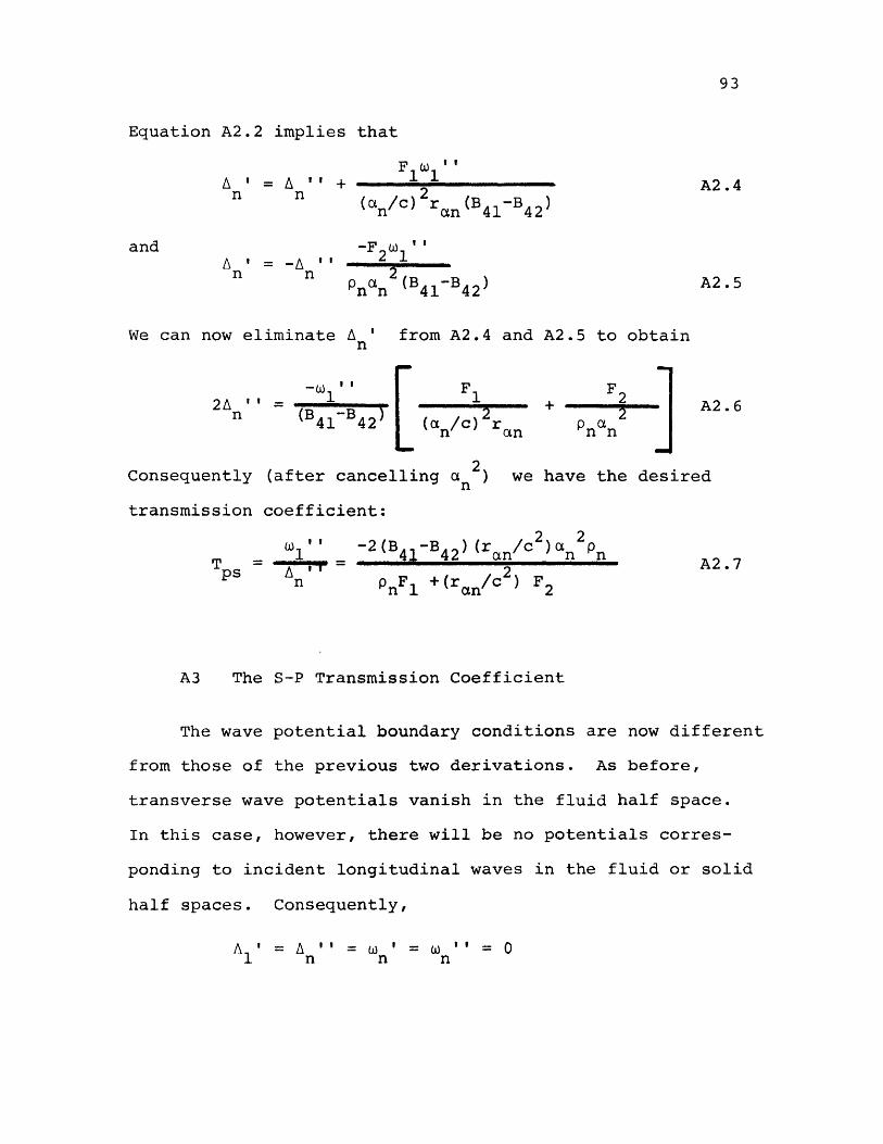
93
Equation A2.2 implies that
A ' = 2 ' + A2.4n n ( n/c)2r an(B -B42
and -F2 1
n n n an2(B 41 -B42 ) A2.5
We can now eliminate A ' from A2.4 and A2.5 to obtainn
-W [ F F 12An (B 1-B ) )2 + a A2.6
n ( 41-B42) (ca /c) r pt ~~ ])[(n/ an n n
Consequently (after cancelling a 2) we have the desired
transmission coefficient:
)( / 2 2oW' -2(B -B42)(ran/c 2)an 2n
Tps =_M=_c2 A2.7
n pnF +(ran/c 2
A3 The S-P Transmission Coefficient
The wave potential boundary conditions are now different
from those of the previous two derivations. As before,
transverse wave potentials vanish in the fluid half space.
In this case, however, there will be no potentials corres-
ponding to incident longitudinal waves in the fluid or solid
half spaces. Consequently,
A n o n n = W nt 0
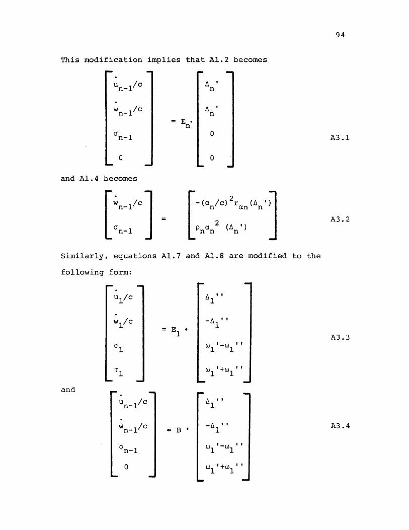
This modification implies that Al.2 becomes
= E -
0
0
A3.1
and Al.4 becomes
2a /c) r
P n nw cxn-1
Cn-1
A ')n
A3.2
Similarly, equations Al.7 and Al.8 are modified
following form:
A1
-A
Wl 1
+W
A ''
-1 ''
-A
W1 -1
W 1 1+W 1'
to the
A3.3
A3.4
un-1
wn-1
u1/c
./c
and
n/cn-1 /
n-1 / = B *a

Therefore,
- (an/c) 2ran An
Pn anAn
0
B21 B22 B23 B24
B31 B32 B33 B34
B B B B
A1 ,
-A
1'1
W 1 '1 + 1 1
Expanding A3.5 produces three equations which can be solved
for the desired potential relationships.
A' ''(B 41-B42 + 1'(B 4 3 +B 4 4 ) - W1 ' '(B 4 3 -B 4 4 ) = 0 A3.6
-(an/c) 2r an n A ''(B21-B22 + W1 '(B23+B)24 l ' '(B23-B24)
A3.7
nan n A1 ' (B3 -B3 ) + 3 1 '(B 3 +B 3 ) - 1 3(B3 -B 3 4 ) A3.8
Equation A3.6 produces the following identity for o ''.
A' ' (B 4 1 -B4 2) + W, (B43+B )1 (B 4 3 -B 4 4 )
A3.9 can now be substituted into A3.6 and A3.7 to give
A3.9
2~n n A'=
~'2 + W 'F3
(B 43- B44)A3.10
2 -A 3F +W 'F4-( /c an n (B 4-B 44
95
A3.5
andA3.ll
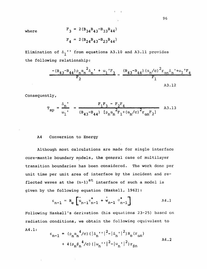
96
where F 3 = 2(B34B43-B33B44 )
F4 = 2(B24B43-B23B44 )
Elimination of A '' from equations A3.10 and A3.ll provides
the following relationship:
-(BAn 3 (4344 w'F ( -B) 43 B n/c) 2 r A n'+w 'F
F2 F1
A3.12
Consequently,
An' F F3 - F2F4Ts == 2 2 A3.13
l' (B43-B 44) [pnan F1 +(a n/c) ranF2
A4 Conversion to Energy
Although most calculations are made for single interface
core-mantle boundary mIodels, the genpral case of multilayer
transition boundaries has been considered. The work done per
unit time per unit area of interface by the incident and re-
flected waves at the (n-1)st interface of such a model is
given by the following equation (Haskell, 1962):
e =R u T + w G A4.1n-l e Lun-1 n-l n-l n-1]
Following Haskell's derivation (his equations 23-25) based on
radiation conditions, we obtain the following equivalent to
A4.1: =: ( 4 AV112.IA 2 )R(rn - l n n / c ) ( | n n , e ( a n
+ 44/ c) o ,, 2_ n , 2) A4 .2

97
The terms in A n''2 and w n 2 represent power fluxes due
to incident P and SV waves respectively across a unit area
of interface. Likewise, the power carried off by the reflected
2 2P and SV waves is given by the terms in JA 'l and 1o 'l.nn
No mode conversion occurs in the case of P to P reflection
in the outer core. Consequently, Al.18 also represents the
square root of the incident to reflected P-wave energy ratio.
Mode conversion takes place during both of the transmissions,
however. Equation B2 enables us to obtain the factors pre-
requisite to converting T P and TSP to square root of energy
ratios.
Consider the case of n = 2 in Figure A2. An arbitrary
interface (labeled "0" and dashed in this figure) is construc-
ted in the homogeneous solid half space. The energy incident
on this imaginary interface is equal to the energy transmitted
through the first interface. Therefore, equation A4.2 can be
employed to obtain the following relationships for a P-wave
incident in the fluid half-space:
C 0 =P 1ayt1 /c(|A 1 ''| ,2 2R e(ral)+4(p16 4 /c)(lo1 ''12_1 , o2)r a
A4.3
6 1 =P 2 a2 4/c(jl l'' 2_Ail 2 )R e(r al)+4(p 2 2 4/c)(o2, 112_1 2'1 )r S2
A4.4
These two equations provide the necessary relationship between
incident and transmitted energy. This relationship is given
in equation A4.5:
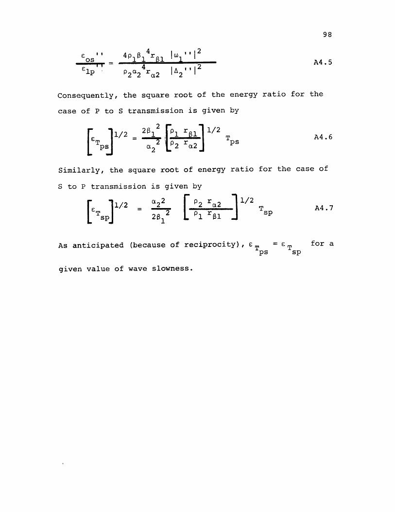
98
E '' 4p 1 1 4r lo ''I- 2 A .4 = 2 A4.5
lp p2a2 ra 2 J 2 1
Consequently, the square root of the energy ratio for the
case of P to S transmission is given by
[T 1/2 _ 2: 2 1/2 T A4.6ET -- p r pS
ps aX2 2 a2l
Similarly, the square root of energy ratio for the case of
S to P transmission is given by
Ts 1/2 22 p2 r 2 1/2 A47T2 P sp
As anticipated (because of reciprocity), e T = T for aps sp
given value of wave slowness.

TABLE Al
pn = density
d = thicknessn
y , yn = Lamd elastic constants
an = P-wave velocity
Sn = S-wave velocity
K = p/c = wave number
r = +[(c/an ) 2 _ 111/2 c>an
-i[l - (c/an 2 J1/2 c<an
r +[(c/Sn 2 - 111/2 c>
-i[l - (c/sn 2 1/2 c<n
nn n( Cy = 2(Sn/c)2
u,w = displacement components in x and z directions
a = normal stress
T = tangential stress

100
FIGURE CAPTIONS
Figure Al
Figure A2
Notation for wave potentials used in deriving
CMB reflection and transmission coefficients
Model notation used in deriving energy
relations
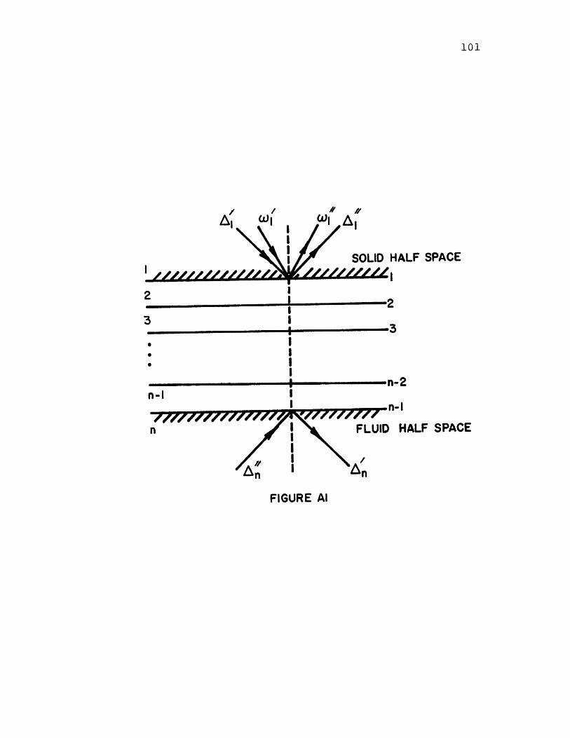
101
/ A,
A
SOLID HALF SPACE
n-2n-3
n-I
FLUID HALF SPACE
FIGURE Al

102
0
I SOLID HALF SPACE
2
n-I
n FLUID HALF SPACE
FIGURE A2