corporate financing under ambiguity: a utility-free ... · corporate financing under ambiguity: a...

Corporate Financing under Ambiguity: A Utility-Free

Multiple-Priors Approach

Chang-Chih Chena

First Draft: May 2011

This Draft: October 2012

Abstract

I build a novel utility-free ambiguity model using the misspecification of probabilities

within good-deal price bounds. In the model managers and outside investors both feel

uncertain about the compensation for invisible idiosyncratic shock on firm’s partially-

tradable assets, and infer the magnitude of ambiguity from arbitragers’ ambition. This

ambiguity model is applied to a contingent claim-based capital structure framework. I

find ambiguity aversion makes lenders hold a most pessimistic belief about the firm’s

operating performance as well as their default decision. This key feature helps address

low-leverage puzzle and credit spread puzzle about corporate debts, and highlights the

relevance of ambiguity preferences in measuring hedging demand and agency conflict

beyond debt service. The comparative statics offer an ambiguity-based explanation for

the link between corporate default/financing policies and exposures to systematic risk.

The magnitude of ambiguity aversion effect in explaining the patterns observed in the

capital structure data is also assessed using a large cross section of S&P 500 firms.

Keywords: ambiguity aversion; Sharpe ratio; optimal leverage; credit spread; agency

conflicts; systematic risk.

JEL classification: G32, D81, G13, G33

a Chang-Chih Chen is currently assistant professor from Department of Finance, Shih-Chien University, Kaohsiung Campus, No. 200, University Rd., Neimen District, 84550. Kaohsiung, Taiwan. Tel.: +886 7 6678888 ext. 5114. Email: [email protected]

1

1. Introduction

Since Modigliani and Miller (1958), how firms make optimal financing decisions has

received considerable attention from financiers and economists.1 Corporate financing

accompanies a variety of important issues; e.g., default decision, capital structure, risk

management, debt valuation, agency conflicts, etc. Unless a very little literature on the

bond pricing subject to information uncertainty (Duffie and Lando, 2001; Davis, 2008;

and Boyarchenko, 2012), most existing theories are consistently based on the rational

expectation equilibrium with complete information structure. In this way there leaves

no role for ambiguity (or uncertainty) to play within the analytical frameworks.

The relevance of aversion to ambiguity in the contexts of decision-making, how-

ever, has been widely documented.2 Knight (1921) firstly defines ambiguity as a case

where informational-constrained agents are uncertain about probability measures used

for decision making. The Ellsberg Paradox (Ellsberg, 1961) and related experimental

evidences document that the distinctions between risk and ambiguity are behaviorally

meaningful. Several recent studies (e.g., Ju and Miao, 2011) conclude that the rational

expectation hypothesis faces serious difficulties in confronting with asset market data.

For these reasons, this paper aims at providing a first step towards understanding and

assessing the impact of ambiguity aversion on the features of corporate financing.

I propose a novel utility-free multiple-priors approach to model ambiguity using

the misspecification of probabilities within “good-deal” price bounds of Cochrane and

Saa-Requejo (2000). My model departs from the traditional max-min model of Gilboa

1 See, for example, Jensen and Meckling (1976), Miller (1977), Myers (1984), Leland (1994), Leland and Toft (1996), Leland (1998), Morellec (2001), Ju et al. (2005), Hackbarth et al. (2006), Bhamra et al. (2010a, 2010b), Carlson and Lazrak (2010), Chen (2010), and He (2011). 2 The impacts of ambiguity aversion on decision-making have motivated a vast literature on financial economics. Part of this literature devotes to explaining the puzzles of interest rates and equity premium in the unified framework with a plausible risk aversion parameter (e.g., Epstein and Wang, 1994; Chen and Epstein, 2002; Maenhout, 2004; Leippold et al., 2008; and Ju and Miao, 2011). Another part of this literature puts emphases on the implications for option markets and on the distinct portfolio behavior of ambiguity-averse investors; such as Epstein and Miao (2003), Liu et al. (2005), etc.. Gagliardini et al. (2009) study the implication of ambiguity aversion for the term structure of interest rate.

2

and Schmeidler (1989) and smooth model of Klibanoff et al. (2005) in two aspects: (i)

it uses the quasi arbitrage (good deals)-free condition to determine the magnitude of

ambiguity exogenously; and (ii) it permits the explicit separation between information

constraint, measured as the proportion of systematic risk to total risk, and ambiguity.

Due to the freedom from estimating the abstract parameters in a utility function

(e.g., intertemporal substitution elasticity or risk aversion), and from concerning about

heterogeneity among various types of preferences, my model is much more tractable

for empirical assessments. The model still offers empirical research a useful guide to

construct the proxy variable of economic uncertainty using the upper limit of market’s

Sharpe ratios, which can be easily measured. On the other hand, constructing such a

proxy variable with the use of traditional models may fail to hold consistency, because

the endogenous form of ambiguity is jointly dependent with the structure of decision

problems and with the shape of decision makers’ subjective utility. Besides, my model

allows for analyzing the comparative statics with respect to informational constraint.

It thus can be applied to explaining the link between systematic risk exposures and the

cross section of corporate decisions (Acharya et al., 2012; and Chen et al., 2012), or

between systematic risk exposures and the price structure in derivative markets (Duan

and Wei 2009). Most importantly, my model is more suitable for examining the firm-

based decision behavior. The reason is that working on prior models shall be restricted

by a standard assumption that all the economical agents share a unique utility function.

This assumption seems convenient but inconvincible especially for corporate decision

making with multiple planners that could be affected by utility heterogeneity.

I embed my new ambiguity model inside the Leland’s (1994) contingent claim-

based capital structure framework. I explore the empirical implication of this modified

capital structure model in two ways. First, I use the basic calibration to quantitatively

study how lenders’ aversion to ambiguity over the assets’ return affects the features of

3

corporate financing. I find that ambiguity aversion (i) makes managers choose a lower

bankruptcy-triggered threshold such that the downside distortion in the expected asset

price is less likely to fully offset the default loss suffered by lenders; (ii) makes firms

use less debts and pay more interests for debt service simultaneously; (iii) discourages

managerial risk-shifting incentives, leading to a weaker hedging intention and asset-

substitution effect; (iv) benefits lenders by saving their hedging cost and by mitigating

agency conflicts; and (v) has an increasing first-order impact but decreasing marginal

effect on the decision rules, given a rising degree of information constraint.

Second, I use a large cross section of S&P 500 firms to assess the magnitude of

ambiguity aversion impacts within the present model. The structural estimations show

that on average, ambiguity aversion explains 22.8% of low uses of financial leverage,

produces 185 bps yield spread without raising leverage, modifies 8.9% (4.5%) of over

-prediction on the equity (debt) value-risk elasticity, cuts one third net tax benefit, and

lowers 21% default boundary. The importance of ambiguity aversion in improving the

goodness-of-fit of the model with respect to leverage, yield spread, and value-to-risk

elasticity is documented using prediction-error tests and moment comparisons.

Next introduce the basic structure of my ambiguity model. I build the model on a

key assumption that the representative firm’s assets are partially-tradable such that the

return cannot be perfectly replicated from well-diversified market portfolio.3 Because

continuous observation on the fundamental value of a thinly or non-traded asset is un-

achievable, public market information is insufficient for firm’s managers and outside

investors to exactly measure the asset return. Information constraint makes them have

heterogeneous beliefs on uncertainty over the compensation for assets’ unobservable

3 Typical intangible assets are often thinly or non-traded, including human capital, trademark copyright, and product-design patents. Korteweg and Polson (2010) document that credit spreads on firms having large intangible assets are the most affected by model uncertainty. See Strebulaev (2003) and Khandani and Lo (2011), for more evidences of asset illiquidity.

4

idiosyncratic risk. Such heterogeneous beliefs are described as a set of approximating

asset-return models under subjective risk-adjusted measures.

Both managers and outside investors use these distorted asset models to trade all

the claims on firm within the good-deal bounds of Cochrane and Saa-Requejo (2000).

The value bounds reflect the upper limit of Sharpe ratios in the open markets, which

corresponds to an upper constraint on the volatilities of stochastic discount factor (see

Hansen and Jagannathan, 1991). In this way pure arbitrage opportunities that deliver

too high Sharpe ratios are precluded.4 The actual trading value relies on the investor’s

subjective belief about model uncertainty as well as his ambiguity attitude. Only when

the 100% systematic risk proportion is given to eliminate informational constraint, the

preference to ambiguity cannot interfere into the decision making such that the model

is degenerated as a standard preference-free type. In the model information constraint

serves as a channel to deliver the ambiguity-related effect on the decision rules; while

its degree acts as a control valve for this channel.

The straightforward implication of my ambiguity model is: due to the constraints

on learning information about the asset value, agents feel uncertain about the expected

asset performance in making the decision. This idea echoes with traditional ambiguity

theories (such as the max-min expected utility theory and smoothness theory), which

interpret ambiguity as a case where the agents are uncertain about probability measure

used for decision making due to cognitive or informational constraint. My idea is also

related to the robustness theory developed by Hansen and Sargent (2001) and Hansen

et al. (2006). Specifically, agents in my model fear the misspecification of probability

assigned to the status of asset performance. Thus they behave pessimistically to avoid

model misspecification when seeking a robust decision making.

4 There is a long tradition in finance that regards the trading with high Sharpe ratios as a pure arbitrage opportunity (see Ross, 1976; Shanken, 1992; Ledoit, 1995; and Cochrane and Saa-Requejo, 2000).

5

The present paper relates to different strands of literature. First, it closely relates

to a growing literature on the bond pricing under uncertainty (Duffie and Lando, 2001;

David, 2008; and Boyarchenko, 2012). So far this line of studies mainly concentrates

on how uncertainty explains the term structure of yield spread, but pays little attention

on how much yield spread is explained by uncertainty, as well as on the endogenous

interaction among bond pricing, hedge intention, and the joint decision on default and

financial leverage. Second, my paper relates to the tradeoff models of Leland (1994),

Morellec (2001), Ju et al. (2005), Hackbarth et al. (2006), Chen (2010), or He (2011).

In these papers, uncertainty over the firm’s growth or performances has been largely

ignored. Third, my paper relates to the vast literature examining the rules of decision

making subject to ambiguity preference. Different with this literature that often works

on asset pricing (e.g., Chen and Epstein, 2002; or Ju and Miao 2011), dynamic asset

allocation (Liu et al., 2005), and the term structure of interest rates (Gagliardini et al.,

2009), the present paper represents the earliest example to apply ambiguity theory to

the issues on corporate finance. Another important difference is that the literature con-

siders systematic-type uncertainty over monetary policy, inflation, or macroeconomic

condition; while this paper discusses non-systematic-type uncertainty attributed to the

idiosyncratic shocks on the individual firm’s operation.

My paper also relates to the literature on corporate risk management and agency

theory (e.g., Haugen and Senbet, 1981; Smith and Stulz, 1985; Campbell and Kracaw,

1990; Leland, 1998; and Aretz and Bartram, 2010). I advance this literature by adding

the effects of lenders’ aversion to ambiguity to the analysis on the positive interaction

between managerial risk-taking incentives and hedge benefit. Such an extension helps

understand whether the ignorance of ambiguity aversion explains the theoretical over-

statements on corporate hedging intention (Guay and Kothari, 2003), as well as asset-

substitution agency problems (Graham and Harvey, 2001). Finally, my paper relates to

6

a recent work by Chen et al. (2012), who studies the implications of the exposures to

systematic risk for corporate credit spreads and default/financing policies. My results

on the comparative statics with respect to information constraint indirectly provide an

ambiguity-based explanation for the relation between systematic risk exposure and the

cross section of corporate capital structure.

The remainder of the paper is organized as follows. Section 2 develops the utility

-free multiple-priors model. Section 3 combines the Leland’s (1994) capital structure

model with the proposed new ambiguity model. Section 4 and 5 respectively presents

the quantitative and empirical results. Section 6 discusses the motivation for potential

lenders to display ambiguity aversion. Section 7 concludes. Proofs, model extensions,

and data technical procedure are available in appendices.

2. A Utility-Free Multiple-Priors Model

Consider a continuous-trading economy endowed with a complete probability

space 0( , , ( ) , )t tΩ where Ω denotes the finite state space, is reference belief,

and continuous filtration 0( )t t supports a two-dimension standard Brownian motion

[ ( ) , ( )]B t W t that generates uncertainty over this economy. Time is continuous and

varied over [0, ) . To fix the term structure of interest rates, assume that default-free

bonds are allowed for trading and pay interests at a constant rate 0r .

2.1. The Brief Review to “Good-Deal” Asset Price Bound Theory

In this subsection, I firstly make a brief review to the theory of “good-deal” asset

price bounds. Extending the incomplete-market setting in Cochrane and Saa-Requejo

(2000) and Chen et al. (2010), I consider a representative firm that is totally equity-

financed at initial time. The firm’s capital assets are partially-tradable and have a total

value unaffected by capital structure, denoted by V following a diffusion process as:

7

( ) ( ) ( ) ( )V VB VWdV t V t dt d B t dW t (1)

with current value (0 )V V , nonnegative constant appreciation rate V , and non-

negative constant volatility VB (systematic shock) and VW (idiosyncratic shock).

Also consider a perfect-liquid asset, such as S&P 500 index or a well-diversified

market portfolio, S used for twin security of V which has the following evolution:

( ) ( ) ( )S Sd S t S t dt d B t (2)

where ( 0 )S S is the current value, S is nonnegative constant appreciation rate,

and S is nonnegative constant volatility. Notably, the firm’s asset correlation with

market, denoted by 2 2corr ( , ) VB VB VWd S S dV V , never equals 1 unless

0VW . The imperfection in the correlation implies that a non-traded or illiquid asset

cannot be perfectly replicated from its twin security. In other words, information from

open markets is insufficient for both firm’s managers and outside investors to exactly

learn the dynamics of asset value. As a result, it is impossible to perfect hedge in such

an incomplete market, suggesting that B and W must be uncorrelated. Once the

replication is less than perfect, the single price law based on the standard no-arbitrage

pricing argument fails. In this case exactly determining the value of claims on a firm’s

assets is unachievable for whole market participants due to information constraint.

According to Proposition 3 of Cochrane and Saa-Requejo (2000), the stochastic

discount factor of any economic agent is governed by a dynamic process:

2 2( ) ( ) ( ) ( )S Sd t t r dt h d B t h dW t A (3)

In (3), ( )S S Sh r denotes the Sharpe ratio of market index; 2A denotes the

upper limit for volatility; and parameter [ 1,1] controls the range of its variation

to ensure the fulfillment of volatility constraint 2 2E [( ( ) ( )) ]t d t t A . The diffusion

8

term 2 2Sh A and Sh measures the required compensation for idiosyncratic risk

and systematic risk respectively. Thus the lower good-deal bound solves

10 0

(0) min E [ (0) ( ) ( ( )) ]cC s x V s d s

(4)

subject to 10 0(0) E [ ( ) ]tt P X ; ( ) 0t ; 2 2E [( ( ) ( )) ]t d t t A ; for 0 t

where (0)C is the lower good-deal bound; ( )cx is the focus payoff associated with

V to be valued; 0P and tX are the price and payoffs of basis assets (vectors); and

the upper good-deal bound solves the corresponding maximum.

The volatility constraint on the discount factor is at the heart of good-deal pricing

bound theory. Hansen and Jagannathan (1991) interpret the restriction on the discount

factor volatility as an upper limit on Sharpe ratio of mean excess return to standard

deviation. Cochrane and Saa-Requejo (2000) choose 2 2 ShA by assuming that an

investor will chase any opportunity or asset that delivers a Sharpe ratio twice that of

market index. They argue that investors are attracted by good deals—large Sharpe

ratios—as well as pure arbitrage opportunities. The size of 2A , therefore, depends on

the ceiling of Sharpe ratios least required by potential arbitragers. If 2A is chosen at

a higher level, the range of good-deal bounds will be wider, suggesting that investors

display a more conservative intention to arbitrage, and will be more careful in judging

the arbitrage opportunities. In brief, values outside good-deal price bounds signal pure

arbitrage opportunities. If the value above upper bound appears, investors consistently

short sell the corresponded asset, and vice versa. So long as the offer prices are within

good-deal bounds, however, the trading strategies adopted by investors are no longer

consistent. This is because, in such a situation, the implied Sharpe ratios are likely not

high enough for a portion of potential arbitragers, but still are regarded as good-deals

by some investors with lower discount factor volatilities.

9

2.2. Model Misspecification within “Good-Deal” Asset Price Bounds

Using the change from real measure to risk-adjusted measure with discounter

( ) e rtt , I follow Cochrane and Saa-Requejo to rewrite the reference model (1) as

ˆ( ) ( ) ( ) ( ) ( )V VB S VW VB VWd V t V t h h dt d B t dW t . (5)

Notice that, only when the agent guesses the true compensation for unobservable idio-

syncratic shock h , the drift of (5) can be reduced as risk-free interest rate r. Because

continuous observation on the fundamental value of firm’s partially-tradable assets is

unachievable, however, public market information is insufficient for agents to exactly

measure the asset return as well as the fair risk compensation. Due to this information

constraint, the agent must subjectively choose the compensation for idiosyncratic risk

2 2 ˆSh h h h A from a set of distorted risk-adjusted drifts 2 2 2 : Sh h h A

when modeling the data-generating process of asset return.

The agent in fact uses an approximating asset-return model

ˆ( ) ( ) [ ( ) ] ( ) ( )h hV VB S VW VB VWd V t V t h h h dt d B t dW t (6)

in determining the price of the contingent claims on firm within good-deal bounds

1 10 00 0

(0) E [ (0) ( ) ( ( )) ] E [ (0) ( ) ( ( )) ]c h cC s x V s d s s x V s d s (7)

where h represents absolutely continuous contaminations with respect to reference

risk-neutral belief ; 0E ( )h is the expectation operator at time-0 under measure h ;

hB B is a standard Brownian motion under h ; hW follows a form of measure

change similar to the transformation of probability scenario mentioned by Epstein and

Miao (2003), Liu et al. (2005), or Gagliardini et al. (2009): 0

( ) ( )thW t W t h d s ;

and h is the contaminating drift that satisfies good-deals (arbitrage)-free condition:

2 2 2ˆ( ) ( )S S Sh h h h h A . (8)

10

Hence ambiguity takes the form of the changes of expected appreciation in the asset

value under a set of distorted risk-adjusted measures.

2.3. Measuring the Model Misspecification: Discounted Relative Entropy

The bound (8) is useful for measuring the range of discrepancy between the true

model (1) and distorted model (6). According to the robustness theory of Hansen and

Sargent (2001) and Hansen et al. (2006), the discounted relative entropy is defined as

00( ) E ( log ( )) ( )hh m t d t

where ( )m is the Radon-Nikodym derivative of

with respect to h . Given 0

( ) ( )thW t W t h ds ,

0

ˆ( ) ( )t

W t W t hds , and

2

0 0( ) 2

( ) et thhd W s h d s

m t

, we thus can derive the model-misspecification constraint as

1

0( ) 0.5( ) ( ) 0.5( )S S S Sh h h t d t h h r

(9)

In the specification-error constraint (9), describes the magnitude of ambiguity

aversion displayed by an agent. It is jointly determined by the Sharpe ratio of market

index Sh , the upper bound for Sharpe ratios in the market 2ShA , and the risk-free

interest rate r . An extended implication behind constraint (9) is that the preference of

agents to ambiguity is related to economic scenarios. Brennan et al. (2001) document

that recessions are often associated with a growing market Sharpe ratio. Perez-Quiros

and Timmermann (2000) and Whitelaw (1997) both found similar cyclical patterns in

the Sharpe ratios. On the other hand, the upper limit on the observable Sharpe ratios

reflects investors’ ambition to arbitrage as well as the condition of cash holding. If the

cash holding is insufficient, investors would display a more conservative intention to

arbitrage such that more high-Sharpe-ratio assets are left in the market. Kato (2006)

finds pro-cyclical corporate demands for liquid assets. Chen (2010) argues that firms

hold more cash in good times because of lower marginal cash cost. Briefly speaking,

11

within the model agents infer the magnitude of ambiguity from the signal of economy

state. As the observed economy state deteriorates, the magnitude of model uncertainty

increases such that the ambiguity-based impact on the decision rules gets stronger.5

2.4. Max-Min Infinite Value Program under Ambiguity Aversion

Next consider the decision program of managers of the representative firm under

ambiguity. In making the financing policies, the subjective belief managers hold about

uncertainty over the asset’s return depends on the attitude of external bond investors

toward ambiguity. In order to restrict our attention to the central issues, assume that

potential lenders faced by managers are ambiguity-averse. For simplicity, also assume

their knowledge about Sharpe ratios in the market is symmetric.6 Thus the preference

of ambiguity aversion forces managers to hold a most pessimistic belief on the future

asset return. In the later section I will explain why lenders prefer ambiguity aversion

to ambiguity loving from the arguments concerning bond hedge and agency conflict.

One important thing we must notice when defining managers’ objective function

is that the changes in the fundamental value of firm’s total assets cannot be observed

continuously. Managers only conjecture the asset value at ( ) E ( ( ))hh tV t V t based on

the public information during the period of debt service. This conjectural asset price

offers managers an alternative criterion to consider the decision on default. It is jointly

determined by the realized market index return and managers’ subjective belief about

model uncertainty: with (0)h hV V V ,

2 2 1 1

0 0( ) exp [ ( 1 ) 0.5 )] ( ) ( ).

t t

h V V VB VB S S VB SV t r h h du dS u S u V

As suggested by the Ellsberg Paradox, an ambiguity-averse agent behaves as if 5 Korteweg and Polson (2010) and Boyarchenko (2012) similarly document that the amount of model misspecification and of uncertainty about asset pricing increases during the 2007-2008 financial crises. 6 The assumption of symmetric-information structure is unnecessary, but makes models more tractable. In appendix I will extend the model to include informational asymmetry between managers and lenders to show that my basic results do not rely on the assumption of information structure.

12

he maximizes his expected utility under a most pessimistic belief chosen from the set

of conditional probabilities (Epstein and Schneider, 2008). Following this notion, the

objective of managers is thus to solve a max-min infinite value program

0 0( )max min E [ ( ) ( , ; ( ) ) ]h

hhx

t L h x V t dt

(10)

2 ( ) ( ) [ ( 1 ) ] ( )hh h V S V Vsubject to d V t V t r h h h dt d B t . (11)

The program (10) is equivalent to the so-called “constrained” robust control problem

in Hansen and Sargent (2001, 2008) and Hansen et al. (2006), and fits the max-min

expected utility theory of Gilboa and Schmeidler (1989). It implicates that ambiguity-

averse managers optimally make the financing strategy x (e.g., debt issuing amount or

coupon level) that maximizes their net leverage value ( )L under a worst-case belief

about asset return chosen from the set of multiple priors ( ) : ( ) h h .7

The role of leverage value here is similar to a utility function in traditional ambiguity

theories. Actually, my model is more tractable for empirical works due to the freedom

from estimating those abstract parameters in a utility function (e.g., risk aversion), and

from concerning about heterogeneity among various types of preferences.

Notably, the time subscript is redundant for the control of the contaminating drift

h . The reason is that, as in Cochrane and Saa-Requejo (2000), both the market-index

Sharpe ratio and the upper limit of observed Sharpe ratios here are treated as constants

calibrated from historical data such that the magnitude of ambiguity is time-irrelevant.

This assumption directly restricts the model’s application to static decision problems.8

The following lemma shows the Bellman-Isaacs condition implied by program (10).

7 See equation (24) for the explicit form of value function of the firm’s net leverage benefits. 8 To relax this assumption, there are at least two ways to capture the time-varying properties of Sharpe ratio. Wachter (2002) models the market price of risk as a mean-reverting process (Ornstein-Uhlenbeck process). Some macroeconomic literature, such as Chen (2010), links the risk price to macroeconomic state, modeled as a Markov-switching jump process. Taking the dynamics of Sharpe ratios into account, however, is redundant for static decision analyses. Because this paper mainly puts the focus on a static capital structure problem, I leave such an interesting extension for future research topics. See appendix for an extended model including dynamic upward capital restructuring.

13

Lemma. Let *( )

( ( ) ) max min E [ ( ) ( , ; ( ) ) ]ht hh thx

F V t s t L h x V s ds

denote the indirect

value of a perpetual claim on the firm’s leverage benefits. Given the dynamics of asset

return as equation (11), the value function F satisfies:

2 2 2 2max min 0.5 ( ) [ ( 1 ) ] ( )

( ) ( , ; ) 0.

h h hV h V V h V S V h V hhx

h h

F r h h h F

r F L h x

V V V V

V V

The Bellman-Isaacs condition above defines an inhomogeneous ordinary differ-

ential equation that has a general solution (see also Leland, 1994; Hansen and Sargent,

2001; and Gagliardini et al., 2009). Since the explicit pricing formula for a perpetual

claim on the firm’s leverage benefits is available, I could solve the max-min program

(10) explicitly. In this way the optimal controls *x and *h can be easily solved using

the first-order and second-order differentiation conditions.

3. Revisiting Leland (1994): Optimal Capital Structure

This section embeds the utility-free multiple-priors model developed in Section 2

inside Leland’s (1994) contingent claim-based capital structure framework.

3.1. Time-Independent Security Model under Ambiguous Beliefs

Following Leland (1994), consider a circumstance where the representative un-

levered firm intends to sell a perpetual debt at the value equal its par. Let ( )hF V be

the price of a claim on the firm’s assets that pays a continuous coupon (rate) C so

long as the firm is solvent. Based on lemma, ( )hF V satisfies

2 2 2 2(1 2) ( ) [ ( 1 ) ] ( ) ( ) 0h h hV h V V h V S V h V h hF r h h h F r F C V V V V V .

The general solution to this ODE can be easily derived as:

1 [ ( , ) ( , )] [ ( , ) ( , )]1 2( ) ( ; , , )a h b h a h b h

h h h hF C r A A F h C V V V V (12)

14

2 2 2 2 2( , ) [ ( 1 ) 0.5 ]V S V V Va h r h h h ;

2 2 2 2 2 0.5 2 2( , ) [ ( ( , ) ) 2 ]V V Vb h a h r ;

where the constants 1 2( , )A A are determined by boundary conditions. I then specify

the associated conditions to obtain the values of debt, bankruptcy cost, and tax shield.

3.1.1. Perpetual Debt

The debt sold by firm carries a perpetual coupon payment c whose level remains

constant until the bankruptcy is declared. For convenience I express the debt value as

( ; , , )hD h c V with suppressing other arguments. Let BV represents an endogenously-

determined level of asset value at which the firm goes to bankruptcy. Once the bank-

ruptcy occurs, only a portion 1- of the remaining asset value can be redeemed by

debt holders. That means,

lim ( ; , , ) (1 )h B

h BVD h c V

VV (13i)

0lim ( ; , , ) ( )

hhD h c c t dt

VV (13ii)

Given equation (12) with letting C c , condition (13ii) yields 2 0A and condition

(13i) implies 1 ( , ) ( , )1 [ (1 ) ] a h b h

B BA V c r V . Thus

1 1 ( , ) ( , )( ; , , ) [ (1 ) ] ( ) a h b hh B h BD h c c r V c r V V V . (14)

3.1.2. Tax Benefits and Bankruptcy Costs

The well-known tradeoff theory has described the significance of tax effects and

bankruptcy loss in determining the optimal capital structure. Tax benefits enjoyed by a

perpetual debt ( ; , , )hTB h c V resemble a security that pays a constant coupon equal

to the tax-sheltering value of interest payment (with setting C c in (12)) so long

15

as the firm is solvent and pays nothing in the bankruptcy. This security also satisfies

the form as (12) with boundary conditions:

lim ( ; , , ) 0h B

hV

TB h c

V

V (15i)

0lim ( ; , , ) ( )

hhTB h c c t dt

VV (15ii)

Condition (15i) reflects the loss of tax benefits once the firm enters into bankruptcy.

Condition (15ii) implicates that, as the bankruptcy becomes increasingly unlikely in

the future, the value of tax benefits approaches the capitalized value of the tax benefit

flow. Given the above two conditions, using (12) gives

1 ( , ) ( , )( ; , , ) [1 ( ) ]a h b hh h BTB h c c r V V V (16)

Bankruptcy costs are the present value of expected loss in bankruptcy, denoted

by ( ; , , )hBC h c V . This pays no coupon (with setting C=0 in (12)), but has the value

equals to BV at h BVV , suggesting that the boundary conditions are

lim ( ; , , )h B

h BVBC h c V

VV (17i)

lim ( ; , , ) 0h

hBC h c

V

V (17ii)

Applying conditions (17i) and (17ii) to general solution (12) yields

( , ) ( , )( ; , , ) ( ) a h b hh B h BBC h c V V V V (18)

3.1.3. Total Levered Value and Equity

The firm’s initial total levered value ( ; , , )L hTV h c V consists of three parts: the

asset value, plus the tax deduction of coupon payment, less the bankruptcy costs; i.e.,

1 ( , ) ( , ) ( , ) ( , )( ; , , ) [1 ( ) ] ( )a h b h a h b hL h h h B B h BTV h c c r V V V V V + V V (19)

The value of equity equals the firm’s total value minus the value of debt:

1 ( , ) ( , ) 1

( ; , , ) ( ; , , ) ( ; , , )

[ (1 ) ] ( ) (1 )

h L h h

a h b hh B h B

E h c TV h c D h c

V c r V c r

V V V

V V (20)

16

3.2. Endogenous Bankruptcy: Smooth-Pasting Condition

Throughout this research I define the random default time on the firm’s assets as

: inf ( 0: E ( ( )) ( , , ))ht Bt V t V c h .9 For simplicity, only the endogenous bankruptcy

case is considered. By using smooth-pasting condition (see e.g., Leland, 1994; Leland

and Toft, 1996; or Hackbarth et al., 2006), the equilibrium bankruptcy-triggered thres-

hold is chosen to maximize the equity’s value, meaning that *BV solves the equation

( ; , , ) 0h B

h h VE h c

VV V . (21)

The solution to equation (21) can be derived differentiating (20) with respect to hV ,

setting this expression equal to zero with h BVV , and solving for *B BV V , which has

* 1 *(1 ) [( ( , ) ( , ) ) (1 ( , ) ( , ))] ( , , )B BV c r a h b h a h b h V h c (22)

In addition to coupon choice c , managers’ ambiguous belief about uncertainty over

the firm’s growth h enters the formula of *BV . In contrast, the existing models (e.g.,

Leland, 1994; Hackbarth et al., 2006; Chen, 2010) typically imply that *BV is based

on the rational expectation equilibrium. This feature leads to important difference in

the effects of ambiguity preference on the debt value between their models and mine.

The bankruptcy conditions can be further analyzed by computing the expected

appreciation of equity around the bankruptcy trigger. Due to 0hVE when h BVV ,

expressing the equity value as a function of hV and using Ito’s lemma can simplify

the appreciation of equity as

2 2 2( ; , , ) (1 2) 0

(1 ) [( ( , ) ( , ) ) ( ( ,1) ( ,1) )]

h hh B h Bh V h V VV V

d E h c E dt

c a h b h a h b h dt

V VV V

. (23)

9 Note that in the definition I use expected price rather than actual price due to the fact that managers cannot continuously learn the changes in the fundamental value of firm’s partially-tradable assets. They can only guess the asset’s value under a distorted belief based on market information during the period of debt services. Thus the occurrence of default time means the moment at which this conjectural asset value firstly fall below the predetermined threshold ( , , )BV c h .

17

The left-hand-side of equation (23) implies the expected change in the equity value at

h BVV . The right-hand-side consists of two parts: (i) the ambiguity-based adjustment

factor ( ( , ) ( , )) ( ( ,1) ( ,1))a h b h a h b h , which reflects managers’ subjective belief

about uncertainty; and (ii) the after-tax coupon expense (1 )c , which represents the

additional cash flow that must be provided by equity holders to keep the firm solvent

at bankruptcy point. The expected appreciation of equity equals to the net cost of debt

services only in the rational expectation equilibrium (when letting =1 and V Sh h ).

Once the preference to ambiguity is involved in the decision on default, the expected

appreciation of equity at bankruptcy point no longer matches the contribution required

from shareholders to keep the firm solvent. This naturally echoes with the breakdown

of rational expectation hypothesis.

3.3. Financial Variables under Optimal Financing Strategies

This subsection intends to derive a firm’s financial variables at optimal leverage

in the presence of ambiguity aversion, including optimal debt ratio, debt capacity, and

yield spread on debt. According to capital structure tradeoff theory, I explicitly define

the contingent payoff of claims on the firm’s net levered benefits as

( ) ( )( , ; ( ) ) 1 ( , , )1h t B tL h c V t c V c h , (24)

which equals the value of tax benefits minus bankruptcy costs. The model solution is

summarized in the following theorem (see Appendix A for a detailed proof).

Theorem. Given the max-min objective as program (10), the dynamics of asset return

as equation (11), and the functional form of leverage value as expression (24), ambi-

guity-averse managers choose the coupon and bankruptcy-triggering threshold at:

* ** * * * 1 ( ( , ) ( , ))[ (1 ( , ) ( , ) ) ( , ) ] a h b hA hc a h b h l h V ,

18

* * * * 1 * * * *( , , ) (1 ) [( ( , ) ( , ) ) (1 ( , ) ( , ))]B A AV h c c r a h b h a h b h ,

under the most pessimistic belief about asset return * 2 0.5( )S Sh h h .

The value of whole firm, debt, and equity at optimal leverage are as follows:

* ** * 1 * * * 1 ( ( , ) ( , ))

* * 1

( ; , , ) 1 [(1 ( , ) ( , )) ( , ) ]

[1 (1 ( , ) ( , )) ]

A a h b hL L h A hTV TV h c r a h b h l h

a h b h

V V,

* ** * 1 * * * 1 ( ( , ) ( , ))

* * 1 * * 1

( ; , , ) [ (1 ( , ) ( , ) ) ( , ) ]

[1 ( , ) ( , ) (1 ( , ) ( , )) ]

A a h b hh A hD D h c r a h b h l h

k h l h a h b h

V V,

* * * * * *( ; , , ) ( ; , , ) ( ; , , )Ah A L h A h AE E h c TV h c D h c V V V ;

where

1 1 ( , ) ( , ) 1( , ) [ (1 ) (1 (1 ( , ) ( , )) ) ] [1 ( , ) ( , )]a h b hj h r a h b h a h b h

1( , ) [1 (1 ) ( ( , ) ( , )) ( , ) ( , ) ] ( , )l h a h b h a h b h j h

( , ) [1 (1 ) (1 ) ( ( , ) ( , )) ( , ) ( , ) ] ( , )k h a h b h a h b h j h .

Optimal debt ratio represents the most ideal leverage choice for a firm, equaling

the ratio of debt value to total capital; namely, A A ALL D TV . An important issue that

arises here is whether optimal leverage chosen by managers is lower in the presence

of ambiguity aversion. If the answer is positive, the preference to ambiguity would be

justified in explaining the so-called “under-leverage puzzle”.

The coupon rate can be straightforwardly computed from dividing the coupon by

debt value: * * * * * 1 * * 1 1( ; , , ) [1 ( , ) ( , ) (1 ( , ) ( , )) ]A h Ac D h c r k h l h a h b h V .

The distance between the rate of coupon and of risk-free interest measures the yield

spread on debt. The implication of ambiguity aversion effect on the credit spread may

help explain another puzzle-“credit spread puzzle”, if the positive ambiguity premium

does exist given a small leverage.

19

Debt capacity demonstrates the maximal value of debt issued by firm. The target

coupon that maximizes the debt value is derived differentiating *( ; , , )hD h c V with

respect to c, setting the resulting equation to be zero, and solving for maxAc c . Thus

we have * ** * * 1 ( ( , ) ( , ))[ (1 ( , ) ( , )) ( , )]max a h b h

A hc a h b h k h V and debt capacity

* * * ** 1 * 1 ( ( , ) ( , )) * * (1 1 ( ( , ) ( , ) ) )

* *

( ; , , ) [ ( , ) (1 ( , ) ( , ))

( ( , ) ( , ))]

max a h b h a h b hh AD h c Vr k h a h b h

a h b h

V.

4. Quantitative Results

I conduct the numerical analyses to quantitatively study how ambiguity aversion

affects the features of corporate financing, including leverage choice, default decision,

credit spread, debt capacity, agency conflicts, and hedging demand. For comparison, I

use the endogenous case of Leland (1994) as my benchmark model ( 1 ).

4.1. A Basic Calibration

I choose the baseline parameters at the values that roughly reflect a typical U.S.

corporation. I normalize the initial unlevered value of firm’s assets V to $100. While

this value is arbitrary, I show below that neither credit spread nor debt ratio at optimal

leverage depends on this parameter. Because there is no difference in the variance of

return between the firm’s assets and equity, I choose the asset’s aggregate risk V at

20% that is close to the empirical estimate of equity volatility in Cecchetti et al. (2000)

and Chen (2010). I choose the risk-free interest rate r to be 1.47%, which is consistent

with the consumption-based calibrated results of Chen (2010). According to Carlson

and Lazrak (2010), the U.S. firms have the average effective tax rate of 32%. Thus I

use =32% throughout the section. Following Leland (1994), Leland and Toft (1996),

and He and Xiong (2011), I use bankruptcy cost =50% that is close to the empirical

20

estimates of Ju et al. (2005) and Morellec et al. (2011), around 48.52% to 49.1%.

I choose the parameter governing the upper bound for the volatility of stochastic

discount factor 2A to be 2 Sh . Such a choice implies 2 , which suggests that no

portfolio traded in the market has more than twice the market index Sharpe ratio (see

also Ross, 1976; Shanken, 1992; Cochrane and Saa-Requejo, 2000; and Hung and Liu,

2005). I borrow the estimates of Carlson and Lazrak (2010), Chen (2010), and Ju and

Miao (2011) to choose market-portfolio Sharpe ratio Sh at 0.33. I set the correlation

coefficient between the return on the firm’s assets and market index at 0.9, which

is also used by Cochrane and Saa-Requejo (2000). Using the standard CAPM theory,

I derive the asset’s Sharpe ratio under market-based expectation as E ( )V B Sh h .10

4.2. The Decision to Default

I firstly study how managers make responses to ambiguity aversion displayed by

potential lenders in considering the decision to default. In the model managers choose

an optimal bankruptcy-triggering threshold based on the smooth-pasting condition to

make their default policies. Thus I plot the equilibrium bankruptcy-triggered threshold

as well as the expected recovery rate as a function of debt value in Figure 1.

[Insert Figure 1 here]

During the period of debt service, managers just know the subjectively-expected

value of firm’s partially-tradable assets from the public market information. Because

10 Because of informational constraints, the true expected asset return

V is unknown in the economy. Agents can only conjecture the return rate based on public market information. Following such an idea, I therefore apply the standard CAPM theory to the derivation for the market-based expected return rate for assets: 1E ( ) ( E ( )cov ( , ) ) var ( )B BdV V rdt d S S rdt d S S dV V d S S .

21

ambiguity aversion forces managers distortedly hold a worst-case belief on uncertainty

over the firm’s performance, assets are always under-valued in terms of expectation.

Managers learn the actual value of assets in place only through a bankrupt liquidation.

Thus a troublesome problem for managers that arises here is how to determine an ideal

bankruptcy point where the liquidated value of remaining assets left for debt holders is

not too much. Choosing a lower bankruptcy-triggering threshold intuitively could be a

realistic counterplot to such a problem. In this way the under-bias in the expected asset

value is less likely to fully offset the expected loss on the debt’s principal. Indeed, this

idea is confirmed by the pattern of Panel A in Figure 1. As we see, the interference of

ambiguity aversion in the default decision lowers the equilibrium bankruptcy-triggered

threshold, given an arbitrary debt level. Moreover, this negative effect gets stronger as

the rises in the debt’s issuing amount. Therefore, the expected debt recovery rate under

ambiguity aversion is smaller than the standard case without ambiguity (Panel B).


Within the present model, ambiguity aversion affects the subjective probability of

default on the firm’s debt in two ways. The first is that, as shown by Figure 1, it delays

default by lowering the bankruptcy-triggered threshold. On the other hand, it advances

default by making managers’ subjective belief about the asset return more pessimistic.

From Figure 2, we can find that the latter dominates the former. More specifically, the

preference to ambiguity delivers a significant amplifying effect on the term structure

of cumulative default probability. For example, when the coupon level is calibrated to

match the debt value at $50, the total probabilities of default within 50 and 100 years

under ambiguity aversion approach 95% and 100% respectively, whereas those under

the standard case sharply falls to 30% and 50%. This suggests that ambiguity aversion

22

makes lenders pessimistically expect that managers are likely to default earlier.

The reason cumulative default probabilities computed by my model are so high is

highlighted by Panel B in Figure 2. Observe that the shape of distribution of subjective

default probability density is more concentrative in the presence of ambiguity aversion.

Further, the convergence speed of density with respect to the extension of time horizon

is clearly faster. These two features reflect an ambiguity-based clustering effect on the

default density distribution, and as a result, a significant corresponded increment in the

cumulative default probability appears. Due to this clustering effect, the expected time

to default from my model is earlier. Such a result is supported by Boyarchenko (2012),

and echoes with Jaimungal and Sigloch (2010) who argue that in a model of corporate

default, ambiguity aversion plays a similar role to risk aversion but has a distinct effect.

p


Figure 3 plots the term structure of cumulative default probability with different

combination of model parameters. The pattern in Panel A indicates that an increase in

the asset risk always leads to a higher default probability, in line with the findings of

prior literature; e.g., Leland (1994) and Ju et al. (2005). Panels B and D consider the

impacts of the changes in investors’ arbitrage intention and market index Sharpe ratio

on default likelihood respectively. The patters in these two panels help clarify how the

shifts in economy state affect a firm’s default policies, because a rising market Sharpe

ratio and more conservative intention to arbitrage both signal recessions (Brennan et

al., 2001; Kato, 2006; and Chen, 2010). As we expect, default probabilities are found

to be inversely related to economy state. The key intuition is that, if the observed state

of economy deteriorates, the degree of ambiguity will increase, resulting in a stronger

ambiguity aversion effect on default. My results can be further linked to the empirical

23

implications of the clustering of default (or credit contagion). For example, Giesecke

(2004) and Driessen (2005) both hold that, when economy enters recession, the shifts

in the aggregate shock increase the likelihood of individual default such that firms in a

common market will default simultaneously. Chen (2010) has a similar simulation of

higher default rates given a worse economy state.

Another interesting detection in Figure 3 is the positive relation between default

probability and assets’ correlation with market (Panel C). From equation (11), observe

that the changes in the asset’s correlation cause a twofold impact on the subjectively-

expected asset return dynamics. On the one hand, with holding a fixed aggregate asset

risk, a weaker correlation implies a lower systematic risk such that the market-based

conjectural asset returns are less volatile. On the other hand, the imperfection in cor-

relation amplifies the negative ambiguity effects on the asset’s expected appreciation

through informational constraint. It seems that the former clearly dominate the latter.

4.3. Optimal Leverage and Debt Capacity

Now examine how lenders’ attitude toward ambiguity affects managers’ decision

on the financial leverage. Figure 4 plots the firm’s total levered value as a function of

leverage. The peak of each curve here represents optimal choice of leverage ratio that

maximizes the tax-bankruptcy tradeoff value on debt issuance. Observe that, relative

to the standard case, both the firm’s total value and optimal leverage under ambiguity

aversion are lower. Such outcomes are attributed to the amplifying effect of ambiguity

aversion on the subjective default probabilities. Precisely speaking, the preference to

ambiguity marginally increases bankruptcy costs but reduces tax benefits on the debt

issuance via default decision. Thus the total levered value enjoyed by a firm becomes

fewer, leading a weaker intention to use leverage. The pattern of Figure 4 also echoes

with the numbers in Table 1, which report that optimal leverage ratio obtained from

24

the benchmark model and mine equals 57.55% and 48.36% respectively.

[Insert Figure 4 and Table 1 here]

We have been aware from Figure 4 and Table 1 that ambiguity-averse managers

will undertake a more conservative debt-issuing strategy when facing uncertainty over

the firm’s performance. I then discuss whether the implications of ambiguity aversion

for leverage usage explain the so-called under-leverage puzzle. This puzzle is initially

highlighted by Miller (1977), who finds that the value of bankruptcy costs alone is too

small to offset the tax benefits of debt, causing the over-prediction for the net value as

well as the usage of leverage.11 Thus the key to address this capital structure puzzle is

to reduce errors in the estimated leverage value by introducing other cost-side factors

into the tax-bankruptcy tradeoff analysis.

Different with existing literature, my key intuition to address the under-leverage

puzzle is based on the lenders’ aversion to economic uncertainty. The intuition is two-

stage. First, ambiguity aversion makes lenders pessimistically force managers assign

higher probabilities to the lower statuses of asset performance. Then, because of the

ambiguity-based amplifying effect on subjective default probabilities, the firm enjoys

a smaller tax benefit but carries a greater bankruptcy cost on the financial leverage. In

sum, I utilize an ambiguity-driven comovement among default likelihood, bankruptcy

cost, and tax benefit to match the observed value of leverage. The well prediction on

leverage value thus naturally helps mitigate the overestimation on leverage choice.

The arguments above can be verified by the numbers in Table 1. It shows that net

tax benefit relative to initial firm value based on my model equals 8.49%, which is far

11 The under-leverage puzzle has motivated a plenty of academic works on agency theory (e.g., Jensen and Meckling, 1976; Myers, 1984; and Leland, 1998), information asymmetry (e.g., Myers and Majluf, 1984), macroeconomic risk (Chen, 2010), and capital structure empirical test (Ju et al., 2005).

25

lower than that of Leland’s model, equaling 13.41%, and much closer to the empirical

estimates, around 6%-9%, of Graham (2000), Korteweg (2010), Van Binsbergen et al.

(2010), and Morellec et al. (2011). My value, however, is still large compared to the

data, because other factors of interest rate risk or macroeconomic shock are ignored in

the modeling. Besides, we note that, comparing with market data in Huang and Huang

(2003) which reports that firms using 53.53% leverage have a 10-year yield spread of

320 bps and default rate 20.6% in average, these values from the benchmark model at

optimal leverage (57.55%) are counterfactually low, equaling 76 bps and 5.56%. But

this puzzling phenomenon disappears after incorporating ambiguity aversion into the

analysis. When leverage is optimally chosen at 48.36%, my model produces the credit

spread and default rate at 279 bps and 4.9% respectively. Huang and Huang (2003)

report those quantities at 194 bps and 4.39%, given leverage ratio of 43.28%.


To understand the sensitivities of optimal leverage ratio to the model parameters,

Figure 5 is provided. Panel A shows that optimal leverage is a decreasing function of

asset risk, consistent with the argument of prior empirical studies that riskier firms do

in fact use less leverage (see, e.g., Titman and Wessels, 1988; and Rajan and Zingales,

1995). The negative slope of lines in Panels B and D suggest that firms facing a worse

economy state are more reluctant to use debts, because a higher market Sharpe ratio

and more conservative intention to arbitrage both imply a larger degree of ambiguity

and are usually accompanied by economic recession. Numbers in Table 1 replicate the

consistency in these facts. When choosing the market’s Sharpe ratio at 0.55 and 0.15,

optimal leverage ratio respectively equals 47.58% and 49.98%. By varying the upper

limit for Sharpe ratios from 3 to 1, optimal leverage ratio climbs to 50.55% from

26

47.38%. My results are in line with Bhamra et al. (2010b) and Chen (2010), who find

that capital structure is pro-cyclical at dates when firms re-lever.

The relation between optimal leverage and the assets’ correlation with market is

considered by Panel C. In the model the correlation serves as a channel to deliver the

ambiguity-related impact on decision-making; while its degree can be conceptualized

as a control valve for this channel. Thus, given a fixed level of ambiguity, ambiguity

aversion effects on optimal leverage will be stronger but marginal effects weaker as

the declines in the correlation. Indeed, such an argument echoes with the pattern in the

figure as well as numbers in Table 1. It is found that the optimal leverage-correlation

line has an increasing positive slope, and optimal leverage ratio reduces from 57.55%

to 46.12%, as the correlation falls from 1 to 0.5.


We now move our attention to the analysis of debt capacity, which represents the

maximum amount of debt that can be sold against the firm’s asset. As argued by much

literature, the variations in debt capacity and optimal leverage are often synchronous

(see, e.g., Leland, 1994; and Asvanunt et al., 2011). Take the rise in asset risk as the

illustration. Debt capacity and optimal debt level for firms with riskier assets both are

relatively lower. Hence, a natural issue that arises here is whether ambiguity aversion

displayed by lenders has identical impact on these two measures of capital structure.

Patterns in Figure 6 help clarify the answer to this issue. It is found from Panel A

that debt capacity implied by my model (equaling $79.27) is clearly smaller than that

by benchmark model (equaling $85.86) due to the ambiguity-based shrinking effects

on the expected time to default. Some interesting behavior of debt capacity is depicted

in Panels B-D. As we see, similar to optimal leverage, choosing a higher market index

27

Sharpe ratio and a more conservative intention to arbitrage both lead to a smaller debt

capacity. These results implicate that the maximum value of firm’s debt that could be

sold in recession is relatively less, in line with the finding of Hackbarth et al. (2006).

Debt capacity and asset-market correlation are positively-correlated, because a weaker

correlation causes a stronger ambiguity aversion effect within the model (see Panel C).

p

4.4. Yield Spread Curves

In this subsection I attempt to analyze the credit spreads on corporate debt. After

calibrating a wide range of structural models to match Moody’s default data, Huang

and Huang (2003) find that those models produce credit spreads well below historical

averages, especially for investment grade bonds. This is so-called credit spread puzzle.

Hence the main challenge to the puzzle is to explain the spreads between investment

grade bonds and treasury bonds. In view of a robust inverse correlation between credit

rating and leverage ratio, I assume, only when the firm uses leverage below 45%, the

debt will be rated at investment grade. To study the implication of ambiguity aversion

for credit spread puzzle, I plot the credit spread as a function of leverage in Figure 7.


Observe from the figure that the preference of ambiguity aversion does generate

a large premium on credit spread, no matter for investment grade or junk bonds. The

premium is still significant even if the leverage is very small (i.e., highly-rated bonds).

The reasons to explain the ambiguity-based premium on credit spread are twofold. On

the one hand, ambiguity aversion causes an amplifying effect on the subjective default

probabilities. On the other hand, ambiguity aversion motivates managers to choose a

lower bankruptcy-triggered threshold such that the expected recovery rate gets smaller.

28

An immediate implication that arises here is: the debt sold by firm is more worthless

in the presence of ambiguity aversion. Hence, given a same coupon level, the implied

coupon rate of my model is higher than the benchmark model. Such results echo with

Duffie and Lando (2001), David (2008), Jaimungal and Sigloch (2010), Korteweg and

Polson (2010), and Boyarchenko (2012), who find that the yield spreads on corporate

bonds and CDS premium are larger after taking ambiguity/uncertainty into account.

I further explore the impacts of ambiguity aversion on the estimations of credit

spread, using Moody’s 10-year default data reported by Huang and Huang (2003) as a

benchmark. According to the market data, a debt issuance accompanied with 48.36%

leverage ratio is probably rated at Baa- or Ba-rating. For consistency in the parameter

choices, I merely take the issuance of Baa-rated and Ba-rated bonds as the illustration.

After calibrating the coupon level to match leverage ratio at 43.28%, and 53.53%, my

model and Leland’s model respectively generates the credit spread at 251 bps and 48

bps for a Baa-rating bond, and 312 bps and 66 bps for a Ba-rating bond. On the other

hand, market data respectively reports the average spread at 194 bps and 320 bps. In

sum, incorporating ambiguity aversion with bond pricing can substantially modify the

biases in the estimation of credit spread.

My estimate of credit spread is higher for highly-rated bonds but lower for junk

bonds compared to market data. The reason is referred to an asymmetric time horizon

effect on credit spread. This asymmetric effect demonstrates that the extension of debt

maturity causes an increasing effect on credit spread when the chosen leverage is low,

but a decreasing effect when the chosen leverage is high (see Leland and Toft, 1996;

Hackbarth et al., 2006).12 Hence, the difference in time horizon between market data

and my model of consol debt naturally highlights discrepancies in the comparison.

12 A similar point is made in Leland and Toft (1996) and Hackbarth et al. (2006). The two papers show that the term structure of credit spread on an investment grade bond is strictly increasing and concave, whereas that on a junk bond has an inverted U-shape.

29


Figure 8 presents the comparative statics of credit spreads. Consider first asset’s

risk. Panel A indicates that credit spread increase with asset’s risk, implying that debt

holders must require additional compensation for default likelihood marginally raised

by the rise in asset risk. Within the present model, variations in the asset’s risk affect

credit spread through debt value. Since higher asset risk often leads to greater default

likelihood, debt on riskier assets is cheaper such that the implied coupon rate is larger.

Consider next the investors’ intention to arbitrage and market index Sharpe ratio.

As argued by my preceding discussion, a higher Sharpe ratio and more conservative

arbitrage behavior both play the signals of recession. Hence, patterns in Panels B and

D, which make responses to Figure 3, suggest that, as economy state deteriorates, debt

value falls and the implied coupon rate goes up due to the rises in default probability

accompanied with the upward-adjustments of ambiguity preference. Such a feature of

model is related to Hackbarth et al. (2006), Bhamra et al. (2010a, 2010b), and Chen

(2010), who found countercyclical credit spreads.

Consider finally the asset’s correlation with market. Notably, this parameter acts

as a “controller” for the effects of ambiguity aversion, not a determinant or factor of

ambiguity. Only when the correlation is less than perfect, the preference to ambiguity

enters the context of decision-making. As a result, the decline in correlation amplifies

the magnitude of ambiguity aversion effect within the model, resulting in an inverse

relation between credit spread and the level of correlation (see Panel C).

4.5. Risk-Shifting Incentives: Asset Substitution Effect and Hedging Intention

Jensen and Meckling (1976) raises a tenet of financial economics that, after debt

30

is issued, shareholders would prefer to increase the riskiness of the firm’s activities.

This is presumed to transfer value from debt to equity, leading to “asset substitution”-

agency problem. The costs of agency conflict intuitively are related to default risk the

debt is exposed to, because as firms are closer to default, shareholders will have less

to lose and tend to pursue riskier investment projects. Leland and Toft (1996) argue

that debt holders must request a higher coupon if shareholders benefit from increasing

the riskiness of firm’s activities. For this reason, the subsection intends to investigate

whether ambiguity aversion affects the agency conflict between shareholders and debt

holders through managerial risk-shifting incentives.


Within the present model, asset aggregate risk consists of two parts: systematic

shock VB and idiosyncratic shock VW . Assume the risk-shifting strategies adopted

by managers are irrelevant with idiosyncratic risk, because it is unobservable and non-

hedgeable. In this way Figure 9 plots the value-to-risk sensitivity for debt, equity, and

whole firm as a function of aggregate asset riskiness. Observe from Panel A that the

sensitivities of equity (solid and dotted lines) are positive whereas those of debt (dash-

dotted and dashed lines) are negative. Such dramatic difference confirms the so-called

asset substitution effect (Leland, 1994; Leland and Toft, 1996; and Ju and Ou-Yang,

2005). This substitution effect disappears as the asset risk approaches 100%, since an

extremely-risky debt is valueless such that no more value can be transferred to equity.

Also observe that the curves of sensitivities under ambiguity aversion (solid and

dashed lines) are clearly flatter than those under standard preference (dash-dotted and

dotted lines). An important implication behind this result is that the value stolen from

debt holders to shareholders through risk-taking strategies is fewer in the presence of

31

ambiguity aversion. In other words, previous capital structure theories that ignore the

preference to ambiguity may overstate managerial risk-taking incentives as well as the

prevalence of asset substitution problem within leveraged firms. The overstatement on

asset-substitution problem has been documented by Graham and Harvey (2001), who

finds very weak evidences of asset substitution effect on capital structure choices.

In the literature on corporate risk management and agency theory, there has been

substantial evidence that firms’ hedging activities are motivated by alleviating agency

conflict (see Haugen and Senbet, 1981; Smith and Stulz, 1985; Campbell and Kracaw,

1990; and Aretz and Bartram, 2010). Leland (1998) and Campello et al. (2010) find

that hedging permits greater leverage and smaller credit spread. DeMarzo and Duffie

(1995) hold that financial hedging improves the informativeness of corporate earnings

as a signal of management ability. The arguments above leave twofold open questions:

Does the preference of ambiguity aversion discourage managers’ hedging intention?

Does uncertainty over asset performance signal the imperfection in hedge? To explore

them, we now turn the attention to Panel B of Figure 9.


From the figure, note that the value-to-risk sensitivities of whole firm are strictly

negative, meaning that undertaking a hedging strategy does increase the firm’s value.

Relative to the case without ambiguity, hedging effect in my base case is quite weak,

and also has a faster convergence speed due to nonhedgeable idiosyncratic risk. More

specifically, in the presence of ambiguity aversion, the firm’s value is less sensitive to

the risk-shifting strategies, causing a smaller hedging benefit.13 The reason corporate

13 Leland (1998) defines hedging benefits as the increases in the firm’s value attributed to the strategies of reducing investment riskiness.

32

hedging under ambiguity aversion is more inefficient lies in the information constraint

on assets’ value, measured by the asset’s correlation with market index ( VB V ).

The patterns in Figure 10 indicate that the hedging effect on the asset’s total riskiness

V VB gets weaker as the declines in the correlation. Only when the information

constraint is released 1 , the perfect hedging efficiency appears. Therefore, given a

same hedging policy or target, the total costs on the risk-shifting strategies in my base

case are naturally higher than those without ambiguity. In sum, within the model there

is a coexistence of ambiguity aversion effect and hedging inefficiency. Changes in the

degree of informational constraint drive an inverse comovement between the hedging

benefit and ambiguity-related impact on the agency conflict. Such an idea echoes with

the argument of above mentioned literature that the effort managers put in the hedging

activities is positively associated with the prevalence of agency problems.

5. Empirical Results

This section assesses the main prediction of my modified capital structure model

illustrated in Section 4 empirically. There are two objectives for empirical analyses. I

firstly measure how big the magnitude of ambiguity aversion effects on the features of

corporate financing are, and then compare the goodness-of-fit of my modified model

with the benchmark model of Leland (1994).

5.1. Data, Parameter Estimations, and Target Variables

I construct a sample of S&P 500 firms covering the period of January 2, 1992 to

December 31, 2011. Since estimating the proposed model requires merging data from

various standard sources, I collect data on stock price and S&P 500 index from 3000

Xtra of Thomson Reuters, corporate bond price from Datastream, and annual financial

statements from Compustat. As in literature, I screen the data on several fronts: (i) all

33

regulated and financial firms are removed; (ii) observations with missing total assets,

market value, long-term debt, debt in current liabilities, and total interest expenses are

excluded; (iii) firms with less than five firm-year observations or 3% book debt-total

assets ratio are eliminated; and (iv) firms which do not appear on the list of S&P 500

components at the end of 2011 are dropped. In addition, I restrict my sample to bonds

with straight type, fixed coupon rate, and no sinking fund options. I also require bonds

sold by the same firm to totally have at least five firm-year observations. As a result

of these selection criteria, my base sample consists of 3980 firm-years for 274 firms

(133 firms have analyzable bond price data). Tables 2 and 3 offer detailed definition

and descriptive statistics for the variables of interest.

[Insert Tables 2 and 3 here]

The estimates of the firm-specific parameters are constructed as follows. I proxy

the aggregate risk on each firm’s asset return using the standard deviation of monthly

return on their equity, given the linear relation between equity value and total assets at

optimal leverage as in Theorem: A ii iE V where 1,2,3, , 274i and

* *1 ( ( , ) ( , ))1 * * *

* * 1 * * 1 * * 1

1 [(1 ( , ) ( , )) ( , )]

[1 (1 ( , ) ( , )) ] [1 ( , ) ( , ) (1 ( , ) ( , )) ].

i i i ia h b hi i i i i i i

i i i i i i i i i i i i i

r a h b h l h

a h b h k h l h a h b h

Notably, despite such a linear relation, one still cannot learn the real asset return from

stock market price exactly. The reason is that the subjective beliefs on the firm growth

implied by price information unceasingly vary with investors’ attitude towards risk or

ambiguity such that the true belief is impossible to be captured. Heterogeneity among

investors’ beliefs, however, will not be involved into the calculation of equity/assets

risk, ensuring the reasonableness of my estimations.

34

I use the Capital Asset Pricing Model in estimating the beta of each firm’s equity

return i . These betas can be used for deriving the firms’ systematic risk proportions

that measure their degree of information constraint; i.e., ii i S V . I calculate the

effective tax rate as dividing the total tax payments by net pretax income. Following

Berger et al. (1996) and Morellec et al. (2011), I estimate bankruptcy costs as:

1 ( ) i i i iTangibility Cash Total Assets

where 0.715 Re 0.547 0.535i i i iTangibility ceivables Inventory Capital . To acquire

the proxy for the Sharpe ratio of a well-diversified market portfolio, I calculate the

ratio of average monthly S&P 500-index excess return to their standard deviation, as

in Duan and Wei (2009). Finally, I use one-year treasury rate as the proxy for riskless

interest rate by following Morellec et al. (2011).

For comparison of the model’s goodness-of-fit, I construct four target variables

by individual firm as follow. Market leverage is computed as the ratio of book debt to

the sum of market capitalization values and book debt. For comparability in the risk-

shifting incentives across firms, I use value-risk elasticity as the proxy for value-risk

sensitivity. Value-risk elasticity of equity (debt) is measured as the coefficient of OLS

regression of stock (bond) monthly return rate on the percentage changes in asset risk.

Longstaff et al. (2005) offer a useful guide to compute corporate spreads. In view

of a fact that less than half of sample firms have sufficient bond data (only 109 firms

have at least two analytical bonds), however, I do not adopt their excellent procedure

to estimate corporate spreads. Besides, it is always impossible to aggregate individual

bond values to obtain the total market value of a firm’s debt, because the low trading

frequency of corporate bonds naturally causes the lack of market-price data. For these

reasons, I proxy Aggregate yield spread by the modified book yield spread, calculated

35

as i i iInterest expense total Book debt Riskless interest rate . Here i is the adjustment

factor for mitigating errors attributed to the refinancing costs, the amortization of debt

discount/premium, and non-debt interest expense.14

Estimating this factor by intra-firm data unfortunately could be unachievable due

to the undisclosed structure of corporate interest expenses. To overcome such a data-

missing problem, I jointly use the merging data on bond yield spread and credit rating

from Huang and Huang (2003) and Chen et al. (2007), and the formulas of S&P 500

corporate spread change of Collin-Dufresne et al. (2001) in calibrating the adjustment

factor (see Appendix C for details). The results on estimation are given in Table 4.

[Insert Table 4 here]

5.2. How Big Are the Impacts of Ambiguity Aversion on Corporate Financing?

The analytical results of Section 4 provide a first step towards understanding the

quantitative impacts of ambiguity aversion on the features of corporate financing. Yet,

these cannot convincingly justify the importance of ambiguity aversion in explaining

the patterns observed in the capital structure data. Therefore, I assess the magnitude of

ambiguity aversion effect within the present model. The results are shown in Table 5.

[Insert Table 5 here]

Observe that ambiguity aversion causes the first-order impacts on both the bond

pricing and leverage choice. On average, ambiguity aversion explains about 22.8% of

14 As suggested by Compustat’s data definition, accounting interest expenses cover not only the actual debt-interest expenses, but also the amortization of debt discount/premium, non-debt interest expenses, and various types of financing charges (e.g., issuing costs). Thus the straight uses of accounting interest expense in calculating the individual firm’s aggregate yield spread must suffer substantial biases.

36

under uses of financial leverage, and generates yield spread of 185 bps without raising

leverage. In particular, these ambiguity-based impacts become stronger within firms

using more leverage, and are robust for firms in different leverage groups. For firms

with leverage lower (higher) than 8% (32%), ambiguity aversion reduces 17% (49%)

of prediction errors on the leverage choice and 49% (66%) of prediction errors on the

yield spread simultaneously. Such a finding echoes with Korteweg and Polson (2010)

who argue that the relation between uncertainty and credit spreads is highly non-linear,

dependent with the level of default risk. Also, it confirms the relevance of ambiguity

aversion in explaining the dual puzzles about corporate debts again.

Now turn the attention to equity and debt value-risk elasticity. As we see, taking

ambiguity aversion into account lowers the firm’s value-risk elasticity. Specifically, it

cuts 0.067 (0.025) value-risk elasticity for equity (debt) on average. While this second

-order effect seems weaker compared to the above two cases, it explains 8.9% (4.5%)

of over-predictions on the equity (debt) value-risk elasticity at optimal leverage. The

negative ambiguity aversion impact on the value-risk elasticity represents a potential

explanation for theoretical overstatements on corporate hedging intention (Guay and

Kothari, 2003) and asset-substitution agency problems (Graham and Harvey, 2001).

Still, it is observed that on average, ambiguity aversion raises 20.15% long-term

(20-year) default probabilities, and reduces 5.5% tax benefits on debts. Jaimungal and

Sigloch (2010) similarly conclude a positive relation between ambiguity aversion and

the probability of corporate defaults. Using the structural estimations, Graham (2000),

Korteweg (2010), Van Binsbergen et al. (2010), and Morellec et al. (2011) report that

the tax benefits of debt broadly equals to 6-9% of initial firm value. The range of this

value is close to my estimate (10.571%) but far lower than that by benchmark model

(16.088%). Overall, ambiguity aversion helps us modify 54-77% of over-biases in the

estimated tax benefits on corporate debts.

37

5.3. Robustness in Goodness-of-Fit

This subsection explores whether the magnitude of ambiguity aversion effects is

sufficient for improving the goodness-of-fit of models with respect to capital structure

data. Two natural methods I adopt to assess the model’s empirical performance are: (i)

to compare various model moments to their empirical analog; and (ii) to examine the

sizes of prediction errors. The comparisons of goodness-of-fit with respect to leverage,

yield spreads, and value-risk elasticity are reported in Table 6, 7, and 8 respectively.

[Insert Tables 6-8 here]

I first give a discussion on the moment comparison. From tables, observe that my

model performs better along moments that the literature has identified to be of first-

order importance. The average and median level of leverage ratio and yield spreads by

my model all are much closer to empirical data, relative to Leland (1994) benchmark

model. Take the case of full sample as an illustration. My model generates the mean

(median) of leverage ratio and yield spread at 48.8% (49.9%) and 262 bps (226 bps)

respectively; Leland’s model generates these at 58.1% (58.7%) and 77 bps (44 bps)

respectively; while real data respectively reports these at 17.6% (15.1%) and 262 bps

(231bps). The same holds true for higher-order moments (i.e., skewness and kurtosis),

except for the case of highly-leveraged firms’ yield spreads. Roughly, the successes of

matching the empirical moments closer are robust for different leverage groups.

Here I consider two standard measures of prediction error, including the mean of

absolute errors (MAE) and the root of mean squared errors (RMSE). In addition, I use

the t-statistic tests for verifying whether the presence of ambiguity aversion mitigates

the prediction errors of the model significantly. The numbers in tables reveal that after

taking ambiguity aversion into account, the model observably has smaller RMSE and

38

MAE. Exactly speaking, RMSE on leverage ratio, yield spreads, and the equity (debt)

value-risk elasticity falls from 0.433, 0.0220, and 0.814 (0.586) to 0.347, 0.0169, and

0.728 (0.545) respectively; while MAE reduces from 0.410, 0.0193, and 0.760 (0.566)

to 0.322, 0.0123, and 0.693 (0.542) respectively. Consistently, the results on t-statistic

test support the hypothesis that incorporating ambiguity aversion into capital structure

models can effectively reduce the errors on predicting leverage level, bond price, and

the sensitivity of equity and debt value to the firm’s riskiness.

6. Why Do Lenders Tend to Be Ambiguity-Averse?

Theoretical results we have discussed are consistently based on a key assumption

that potential lenders are ambiguity-averse. In this section I clarify why aversion is the

preferred ambiguity attitude for lenders from the arguments concerning bond hedging

and agency conflict. For comparability in the analyses, consider ambiguity loving as

the alternative ambiguity attitude. By intuition, I define the preference of ambiguity

loving as a case where the agent behaves as if he maximizes his expected value pro-

gram under a most optimistic belief chosen from the set of multiple-priors. That is,

0 ( ) ( )0( )max max E [ ( ) ( 1 ( , , )1 ) ]h

t B tc h

t c V c h dt

.


We begin with bond hedging. Duration is one of common risk-sensitive measure

for bonds. Macaulay (1938) measure duration as the percent change of a bond price in

response to a uniform change in risk-free interest rates. Following this notion, I plot

duration, 1( ( ) ) ( )D r D , as a function of debt value in Panels A and B of Figure

11. It is observed that, given a same par value, bond duration computed by ambiguity-

39

averse model is strictly shorter than that by ambiguity-loving model. Durations fall as

the increase in debt issuing amount and in implied yield spread. In particular, duration

under ambiguity aversion is concave, but that under ambiguity loving is convex. Such

dramatic differences imply that lenders displaying ambiguity loving have higher out-

lays for duration-matching hedging strategies (e.g., immunization technique). Besides,

this hedging expensiveness is amplified by the rise in the exposure to default risk.

Panel C considers the relation between risk-free interest rate and the changes in

debt value. Observe that the attitude toward ambiguity displayed by lenders has direct

impacts on the reaction of bond price to a change in interest rate. The return on debt

displays a quite weak sensitivity to interest rate under ambiguity aversion, but a strong

sensitivity under ambiguity loving. Since a wider range of variation in bond price due

to interest rate risk requires a more complicated hedging technique, ambiguity-loving

lenders bear higher hedging costs, compared to ambiguity-averse lenders. As a result,

in view of hedging efficiency, lenders prefer ambiguity aversion to ambiguity loving.

Next move the attention to the comparison of agency conflict effects between the

two cases (Panel D). From the figure, note that both the value-to-risk sensitivities of

debt and equity in the ambiguity-averse case are clearly weaker. Such discrepancies in

the sensitivities disappear as asset’s aggregate risk approaches an extremely high level.

These findings reflect a fact that the asset substitution-based agency problem faced by

ambiguity-loving debt holders is more prevalent than that by ambiguity-averse debt

holders. Thus the intention to reduce the costs on agency conflict naturally motivates

potential lenders to be ambiguity-averse.

7. Conclusion

This paper investigates the implications of ambiguity aversion for the features of

corporate financing. To do so, I construct a novel utility-free multiple-prior model by

40

using the probabilistic misspecification within good-deal pricing bounds of Cochrane

and Saa-Requejo (2000). The proposed model represents a significant departure from

the traditional ambiguity theories in two dimensions. First, it exogenously determines

the magnitude of ambiguity using the quasi no-arbitrage condition without specifying

the preferences of decision makers. In this way my model is much more tractable for

empirical assessment due to the freedom from concerning about heterogeneity among

various types of preference, and from estimating those abstract parameters in a utility

function. Second, it measures the information constraint as systematic risk proportion,

independent with ambiguity. Hence, analyzing the comparative statics of the effect of

ambiguity aversion on the decision making with respect to informational constraint is

achievable. Such a feature enables my model to be applied to explaining the relation

between the cross section of corporate decision making and systematic risk exposures.

This paper applies the proposed ambiguity model to Leland’s (1994) contingent

claim-based capital structure framework. The modified capital structure model helps

understand how managers make the response to lenders’ aversion to ambiguity when

deciding the default timing. The model goes a long way to explain the credit spreads

puzzle and low-leverage puzzle about corporate debts from the arguments concerning

ambiguity aversion. The model highlights the relevance of preference to ambiguity in

measuring agency conflict and hedge demand beyond debt services. The comparative

statics of model outputs with respect to information constraint provides an ambiguity-

based explanation for a link between systematic risk exposure and financing decision.

To empirically evaluate the proposed model, this paper uses a large cross section

of S&P 500 firms covering 1992 to 2011. The results show that on average, ambiguity

aversion explains about 22.8% of under uses of financial leverage, generates 185 bps

yield spread without raising leverage ratio, modifies 8.9% (4.5%) of over-predictions

on the equity (debt) value-to-risk elasticity, cuts one third net tax benefits, and lowers

41

21% default boundary. The magnitude of ambiguity aversion effect is large enough to

improve the goodness-of-fit of the model with respect to leverage, yield spread, and

value-risk elasticity significantly.

Much work remains to be done. For example, how the preference to ambiguity

affects the endogenous interaction between firms’ financing and investment will be an

important future research topic. More difficult extensions include capital restructuring

under ambiguity aversion and dynamic utility-free multiple-priors theory.

42

Appendix A. Proof of Model Solution

To incorporate the smooth-pasting condition (21) into decision-making, I begin

the proof by rewriting equations (14), (19), and (20) with *B BV V as

1 ( , ) ( , )( ; , , ) [1 ( ) ( , ) ]a h b hh hD h c cr c k h V V (A.1)

1 ( , ) ( , )( ; , , ) [1 ( ) ( , ) ]a h b hL h h hTV h c c r c l h V V + V (A.2)

1 ( , ) ( , )( ; , , ) (1 ) [1 ( ) ( , ) ]a h b hh h hE h c c r c j h V V V . (A.3)

Recall from subsection 2.4 that the objective of managers is to solve a static max

-min infinite value program as (10). Given the form of net leverage value function as

expression (24), using equation (A.2) thus can rewrite the control problem (10) as

1 ( , ) ( , )

( )max min [ (1 ( ) ( , ) ) ]a h b h

hhc

c r c l h

V . (A.4)

Because the objective function (A.4) is time-independent, I simply solve it with two-

stage method without using dynamic programming technique. At the first stage, the

contaminating drift *h that represents the most pessimistic belief hold by managers

about model’s uncertainty is derived. Then, under this worst-case belief, the second

stage chooses an optimal coupon level *Ac that maximizes total leverage value.

The set of multiple-priors ( )h indirectly defines an inequality constraint

2 ( )S Sh h h . Kuhn-Tucker theorem is thus applicable. However, differentiating the

firm’s value function (A.2) with respect to the contaminating drift h is mathematically

intractable. For this reason, I search *h invoking numerical technique, which gives

* 2 0.5( )S Sh h h . Then plugging *h into the max-min optimization (A.4) and using

the first-order differentiation condition * *1 ( , ) ( , ) *[ (1 ( ) ( , ) ) ] 0a h b h

hc r c l h c V

can solve the optimal coupon choice as

43

* ** * * * 1 ( ( , ) ( , ))[ (1 ( , ) ( , ) ) ( , ) ] a h b hA hc a h b h l h V

The “maximum” property of *Ac is easily verified using the second-order condition

* *1 * * * * * * ( , ) ( , ) 1( ) ( , )(1 ( , ) ( , ))( ( , ) ( , ))( ) 0a h b hh A hr l h a h b h a h b h c V V .

Thus this completes the proof.

Appendix B. Extensions

In this appendix, I extend the base-case model in two dimensions: managers-out-

side lenders informational asymmetry and dynamic capital restructuring.

B.1. Informational Asymmetry

I build the base-case model on a standard assumption that managers and potential

lenders equally have the perfect access to information on Sharpe ratios in the market.

Yet, such an assumption could be too tight, especially for a market having incomplete

information structure. The idea of combining informational asymmetry with a setting

of incomplete market in fact has been recognized by much of literature on information

incompleteness (see, e.g., Duffie and Lando, 2001). For this reason, I discuss how and

whether informational asymmetry between managers and potential lenders affects the

decision-making on debt financing subject to ambiguity preference.

We are easily aware from equation (3) that the incompleteness of information on

Sharpe ratios in the market naturally lowers the observed upper limit on Sharpe ratios

as well as the volatility of stochastic discount factor. Thus information asymmetry can

be modeled as the difference in subjective discount factor. Based on this idea, I rede-

fine the dynamics of stochastic discount factor for managers M and lenders L as:

2( ) ( ) ( ) ( )M M S M Sd t t r dt h d B t h dW t 2A , M M Sh2A ;

44

and

2( ) ( ) ( ) ( )L L S L Sd t t r dt h d B t h dW t 2A , L L Sh2A .

Only if managers and lenders share the same Sharpe-ratio information, their discount

factors will be indifferent; namely, M L . Normally, a longer distance between L

and M implies a stronger degree of informational asymmetry.

Next discuss the impacts of informational asymmetry on the decision-making of

financing. Two possible cases should be considered: (i) M L and (ii) M L . On

the one hand, if Sharpe-ratio information possessed by managers is superior to that by

lenders ( M L ), managers must conceal their information about higher Sharpe ratios

to act in the best interest of equity holders, in view of an inverse relation between the

firm’s net leverage value and the upper limit on Sharpe ratios.15 In this case managers

make the financing decision at L utilizing their informational advantage. On the

other hand, when lenders obtain richer Sharpe-ratio information ( M L ), managers

are forced to take the debt-issuing price with L . Thus summarizing the above two

statements concludes that the upper Sharpe-ratio bound used by managers for decision

making only depends on how much Sharpe ratios in the open market outside lenders

observe, no matter whether their information structure is symmetric or not. Also, it is

understandable that information asymmetry and ambiguity aversion effects within the

present model will move in a same direction, if lenders have better access to Sharpe-

ratio information, and vice versa.

B.2. Dynamic Capital Restructuring

Appendix B.2 shows how the proposed model can be extended to allow dynamic

upward capital restructuring briefly. To do so, let i represents the i-th restructuring

15 The inverse relation between a firm’s net leverage value and the upper boundary of observed Sharpe ratios is available from Table 1.

45

point where 1,2, ,i and 0 0 . By following Leland (1998), Hackbarth et al.

(2006), and Chen (2010), assume that the perpetual debt sold by representative firm at

time point i is callable at par AiP once the subjectively-expected asset value i

hV

firstly reaches the upper restructuring level iUV before the lower bankruptcy-triggered

boundary iBV . At next restructuring time point, a new issue of another perpetual debt

1 1

1 11( ; , , , )

i i

A i ii h UD V c V h

is optimally issued, and a proportional transaction cost for

this new debt issuance 1A

iqP is incurred. Introducing such a transaction cost into the

model helps prevent the firm from restructuring continuously. Therefore, the dynamic

version of max-min infinite value program is given as

1

0 ( ) ( ) ( )( )0

max min E [ ( )( 1 ( , , )1 1 ) ]i

i

i i i i i iiii

h At B t i thc

i

t c V c h qP dt

(B.1)

subject to

2 1( ) ( ) [ ( 1 ) ] ( ) , ( )i

i i h i ih h V S V V h i Ud V t V t r h h h dt d B t V V ,

where

: inf ( : ( ) ( , , ), max ( ) )i i

i

i i i ii i h B h U

s tt V t V c h V s V

;

1 1

1 1 1 11: inf ( : ( ) , min ( ) ( , , ) )

i ii

i i i ii i h U h B

s tt V t V V s V c h

.

The program above seems much more complicated relative to the static program

(10). An effective way to resolve it is to utilize “scaling property”. The reason lies in a

key model feature that the path of optimal contaminating drift chosen by managers is

invariant to the capital restructuring, because ambiguity factors are constant; namely,

0 1 2

* * * 2 0.5( )S Sh h h h h . The path of optimal coupon chosen by managers in

fact is only dependent with assets’ subjectively-expected value. Goldstein et al. (2001)

prove that if two firms are identical except that their initial values differ by a factor,

their levels of optimal coupon, optimal default-triggered thresholds, and all the claims

46

will differ by the same factor. This argument confirms the scaling feature inherent in

my model, because it also holds for a single firm that first issues debt when its value

is 00( )h hV V , and later restructures its capital by retiring all outstanding debt at face

value and then issuing a new larger debt when its value rises to 1 01( )h UV V . In brief,

the scaling property ensures that all period- i claims to firm will scale upwardly by

the same factor i consistently where 0U hV V .

Now derive the model solution. Using the scaling property, program (B.1) can be

reduced as

0 0 0 00

0 0 0

( ),max min ( ; , , , ) ( ; , , , ) ( ; , , , )

U

h U h U h Uhc V

tb c V h bc c V h tc c V h

V V V (B.2)

where 1

00 ( )0( ) E [ ( ) 1 ]

i

ii

h iti

tb t c dt

, 0 00

( ) E [ ( ) ]h i Aii

tc q P

, and

00 0( ) E [ ( ) ( , , ) ]h i

i Bibc V c h

represents the present value of a contingent

claim to the firm’s tax benefits, transaction costs, and bankruptcy costs respectively.

Notably, since the time when either boundary is first hit is random, the prices of these

claims at any point before either boundary is hit do not depend explicitly on time. So I

can apply the general solution (12) to deriving their explicit forms.

Consider first the total value of tax benefits. Two boundary conditions should be

imposed on the general solution:

0

0lim ( ; , , , ) 0h B

h UV V

tb V c V h

and 0 0 0

0 0lim ( ; , , , ) ( ; , , , )h U

h U h UV V

tb V c V h tb c V h

V .

The first defines the condition where the firm declares bankruptcy as usual; while the

other, based on the scaling property, shows that the total tax shield at the restructuring

point 0UV should be as large as it is at hV . Thus a straightforward derivation has:

0 0

0 1 [ ( , ) ( , )] [ ( , ) ( , )]1 2( ; , , , ) a h b h a h b h

h U h htb V c V h c r V V (B.3)

where

47

0 0 0

1 0 [ ( , ) ( , )] 1 [ ( , ) ( , )] 0 11 ( ( ) ( ( ; , , , ) ))a h b h a h b h

U B h UV c r V tb c V h c r V ,

0 0 0

1 0 [ ( , ) ( , )] 1 [ ( , ) ( , )] 0 12 ( ( ) ( ( ; , , , ) ))a h b h a h b h

U B h UV c r V tb c V h c r V ,

[ ( , ) ( , )] 0 [ ( , ) ( , )] 0 [ ( , ) ( , )] [ ( , ) ( , )]( ) ( )a h b h a h b h a h b h a h b hB U U BV V V V ,

and 0

0 1( ; , , , ) ( ) (1 )h U htb c V h tb V V , where

0

1 1 [ ( , ) ( , )] [ ( , ) ( , )] [ ( , ) ( , )] [ ( , ) ( , )]

0 [ ( , ) ( , )] [ ( , ) ( , )] 0 [ ( , ) ( , )] [ ( , ) ( , )]

( ) (1 (

( ) ( ) )) ,

a h b h a h b h a h b h a h b hh h B B h

a h b h a h b h a h b h a h b hU h U h

tb c r V V

V V

V V V

V V

1 [ ( , ) ( , )] [ ( , ) ( , )] [ ( , ) ( , )] [ ( , ) ( , )]( )a h b h a h b h a h b h a h b hh B h BV V V V .

Consider next the total value of bankruptcy and transaction cost. Similarly, these

two claims have the corresponded boundary conditions:

0

0lim ( ; , , , )h B

h U BV V

bc V c V h V

, 0 0 0

0 0lim ( ; , , , ) ( ; , , , )h U

h U h UV V

bc V c V h bc c V h

V ,

0

0lim ( ; , , , ) 0h B

h UV V

tc V c V h

, 0 0 0

0 0lim ( ; , , , ) ( ; , , , )h U

h U h UV V

tc V c V h tc c V h

V .

Their explicit forms are the following

0

0 [ ( , ) ( , )] [ ( , ) ( , )]3 4( ; , , , ) a h b h a h b h

h U h hbc V c V h V V (B.4)

0

0 [ ( , ) ( , )] [ ( , ) ( , )]5 6( ; , , , ) a h b h a h b h

h U h htc V c V h V V (B.5)

where

0

1 0 [ ( , ) ( , )] [ ( , ) ( , )] 03 ( ( ) ( ; , , , ) )a h b h a h b h

U B B h UV V V bc c V h V ,

0

1 [ ( , ) ( , )] 0 0 [ ( , ) ( , )]4 ( ( ; , , , ) ( ) )a h b h a h b h

B h U U BV bc c V h V V V ,

0

1 [ ( , ) ( , )] 05 ( ; , , , )a h b h

B h UV tc c V h V ,

0

1 [ ( , ) ( , )] 06 ( ; , , , )a h b h

B h UV tc c V h V ,

0

0 1( ; , , , ) ( ) (1 )h U hbc c V h bc V V , 0

0 1( ; , , , ) ( ) (1 )h U htc c V h tc V V ,

1 0 [ ( , ) ( , )] [ ( , ) ( , )] 0 [ ( , ) ( , )] [ ( , ) ( , )]( ) ( ( ) ( ) ) ,a h b h a h b h a h b h a h b hh B U h U hbc V V V V V V

and 0( ) Ahtc qPV .

48

Consider finally the value of debt. Applying the two boundary conditions,

0

00lim ( ; , , , ) (1 )

h B

Ah U B

V VD V c V h V

,

0 0

00 0lim ( ; , , , )

h U

A Ah U

V VD V c V h P

,

we have

0 0

0 1 [ ( , ) ( , )] [ ( , ) ( , )]0 7 8( ; , , , )A a h b h a h b h

h U h hD V c V h c r V V (B.6)

where

0 0

1 0 [ ( , ) ( , )] 1 [ ( , ) ( , )] 17 0( ( ) ((1 ) ) ( ) )a h b h a h b h A

U B BV V c r V P c r ,

0 0

1 [ ( , ) ( , )] 1 0 [ ( , ) ( , )] 18 0( ( ) ( ) ((1 ) ) )a h b h A a h b h

B U BV P c r V V c r .

As is typical in practice, I require the debt to satisfy sell-at-par condition. Thus setting

0

00 0( ; , , , )A A

h UD c V h P V solves 0AP as

0

0

1 [ ( , ) ( , )] 0 [ ( , ) ( , )] [ ( , ) ( , )] 0 [ ( , ) ( , )]0

[ ( , ) ( , )] [ ( , ) ( , )] [ ( , ) ( , )] [ ( , ) ( , )] 1 1

((1 ) )( ( ) ( ) )

( ) .

A a h b h a h b h a h b h a h b hB h U h U

a h b h a h b h a h b h a h b hh B h B

P V c r V V

V V c r

V V

V V

Using equations (B.3)-(B.6) has the equity value after the debt is issued, equaling

the unlevered firm value, plus tax shields, less bankruptcy costs, less transaction costs,

less the value of debt,

0

0

0 [ ( , ) ( , )] [ ( , ) ( , )]0 1 3 5 7 2 4 6 8

1

( ; , , , ) ( ) ( )

( 1) .

A a h b h a h b hh U h h

h

E V c V h V V

V c r

The limited liability of the equity must satisfy the smooth-pasting condition:

[ ( , ) ( , ) 1]1 3 5 7

[ ( , ) ( , ) 1]2 4 6 8

[ ( , ) ( , )]( ) [ ( , ) ( , )]

( ) 1 0

a h b hB

a h b hB

a h b h V a h b h

V

(B.7)

Equation (B.7) endogenously determines the optimal bankruptcy-triggering boundary

as a function of coupon and capital restructuring level. Thus plugging the equilibrium

bankruptcy-triggering threshold into program (B.2) rewrites the decision program that

can be used to solve optimal coupon and upward restructuring level numerically.

49

Appendix C. Calibrating the Interest-Expense Adjustment Factor

I adopt a backward recursive method to calibrate the interest-expense adjustment

factor. The calibration is achieved by the following steps.

Step 1: I collect the merging data on credit rating, financial leverage, and yield spread

from Huang and Huang (2003) and Chen et al. (2007). The merging data reveals that

on average, firms rated at AAA have yield spread of 133 bps and 13.08% leverage; at

AA have 21.18% leverage and 152 bps yield spread; at A have 31.98% leverage and

183 bps yield spread; at BBB have 242 bps yield spread and 43.28% leverage; at BB

have 53.53% leverage and yield spread of 437 bps; and at B have 65.7% leverage and

yield spread of 681 bps. The reason I use the yield spread data from Chen et al. (2007)

is that the horizon of their long-maturity (15-40 years) data can well match the present

model of consol bonds without term premium-based modifications.

Step 2: I calibrate the final firm-year adjustment factor for each sample firm 20i at

which the modified book yield spread matches a historical average level corresponded

to their own credit rating. Specifically, for each firm i with current rating j, I solve

,20 ,20 ,20 ,20 20( )

- .

i i i iYS Interest expense total Book debt Riskless interest rate

Rating j avg yield spread

(C.1)

For little firms without credit rating, I artificially assign them to rating AAA, AA, A,

BBB, BB, and B, if their last firm-year market leverage is within the range from 0%

to 17%, from 17% to 26%, from 26% to 37%, from 37% to 48%, from 48% to 59%,

or from 59% to 100% respectively. Then the last firm-year adjustment factors of these

firms can be similarly solved using equation (C.1).

Step 3: I use the formula of S&P 500 yield spread changes from Collin-Dufresne et al.

(2001) to backwardly calibrate each period’s adjustment factor ,19 ,1, ,i i . The goal

is to recursively solve the following system of equation with terminal condition (C.1):

for 2,3, ,19t ,

50

10, , 1

10 10 2, , 1

10 10 2, , 1

0.095 0.014 , if [ 0%,15%]

0.161 0.057 ( ) 0.028 0.015 , if [15%, 25%]

0.156 0.056 ( ) 0.035 0.012 , if [ 25%,3

i t t t i t

i t t t t t i t

i t t t t t i t

YS r SP Lev

YS r r slope SP Lev

YS r r slope SP Lev

10 10 2

, , 1

10, , , 1

10 10 2, ,

5%]

0.2 0.055 ( ) 0.017 , if [35%, 45%]

0.015 0.21 0.013 , if [ 45%,55%]

0.013 0.211 0.143 ( ) 0.088 0.017 ,

i t t t t i t

i t i t t t i t

i t i t t t t t

YS r r SP Lev

YS Lev r SP Lev

YS Lev r r slope SP otherwi

se

(C.2)

In (C.2) , , , 1( ) ( )i t i t i tYS YS YS is the single-period changes in the aggregate yield

spread; ,i tLev , 10tr , 10 2( )tr , and tslope respectively denotes the single-period

changes in market leverage, 10-year treasury rate, the square of 10-year treasury rate,

and the slope of treasury yield curve; and tSP is t-year return on S&P 500 index.

The system of equations above is a little bit different with Collin-Dufresne et al.

(2001). I do not take the changes in the magnitude of downward jumps in the firm’s

value into account, because the impact of jump risk on capital structure choices is not

in the primary attempts of this research. Also, I drop the variables whose explanation

powers are statistically insignificant from formulas (t-stat. within the range from -1.96

to 1.96). While there may exist under biases in the variance of yield spread under such

tractable procedures, my cross-sectional estimates of yield spreads hold unbiasedness,

so long as (i) the final year-end book yield spread matches its historical average level;

and (ii) actual changes in the yield spread are symmetrically distributed.

There are some indications that corporate spread changes approximately follow a

symmetric distribution. Using the descriptive statistics, Campbell and Huisman (2003)

report that shifts in the U.S. corporate spread have -0.052 skewness. Huang and Kong

(2003) particularly discover that the skewness of long-maturity and high-rating spread

changes is closer to zero. The weighted-average skewness of 15-year-and-more yield

spread changes of investment grade bonds equals -0.293; while the spread changes of

51

junk bonds are right-skewed weakly, and have the average skewness of 1.035. Similar

to Huang and Kong (2003), Avramov et al. (2007) show that the mean and median of

changes in investment-grade corporate spread match perfectly, but the mean of spread

changes of junk bonds (0.06) is slightly larger than the corresponded median (0.05).

It is noteworthy that a positive skewness of yield spread changes implies that the

probabilities of negative changes are more than those of positive changes. Hence, my

backward calibration for interest-expense adjustment factor would underestimate the

cross section of yield spread on low-rated firms, if the case of right-skewed junk-bond

spread changes holds true. This indirectly explains why my target yield spreads in the

case of highly-levered firms (equaling 311 bps) are slightly lower than those from the

modified capital structure model (equaling 354 bps). Even though such under biases

weaken (improve) the performance of my (benchmark) model on fitting yield spreads,

the present results on prediction-error tests still support the hypothesis that my model

has better goodness-of-fit with respect to yield spreads (see Panel C in Table 7).

52

References

Acharya, V., H. Almeida, and M. Campello. “Aggregate Risk and the Choice between

Cash and Lines of Credit.” Forthcoming, Journal of Finance, 67 (2012).

Aretz, K. and S. M. Bartram. “Corporate Hedging and Shareholder Value.” Journal of

Financial Research, 33 (2010), 317-371.

Asvanunt, A., M. Broadie, and S. Sundaresan. “Managing Corporate Liquidity:

Strategies and Pricing Implication.” International Journal of Theoretical and

Applied Finance, 14 (2011), 369-406.

Avramov, D., G. Jostova, and A. Philipov. “Understanding Changes in Corporate Cre-

dit Spreads.” Financial Analysts Journal, 63 (2007), 90-105.

Berger, P., E. Ofek, and I. Swary. “Investor Valuation and the Abandonment Option.”

Journal of Financial Economics, 42 (1996), 257-287.

Bhamra, H. S., L. Kuhn, and I. Strebulaev. “The Levered Equity Risk Premium and

Credit Spreads: A Unified Framework.” Review of Financial Studies, 23 (2010a),

645-703.

Bhamra, H. S., L. Kuhn, and I. Strebulaev. “The Aggregate Dynamics of Capital

Structure and Macroeconomic Risk.” Review of Financial Studies, 23 (2010b),

4187-4241.

Boyarchenko, N. “Ambiguity Shifts and the 2007-2008 Financial Crisis.” Journal of

Monetary Economics, 59 (2012), 493-507.

Brennan, M., A. Wang, and Y. Xia. “Intertemporal Capital Asset Pricing and the

Fama-French Three Factor Model.” working paper, UCLA (2001).

Campbell, R. and R. Huisman. “Measuring Credit Spread Risk: Incorporating the

Tails.” Journal of Portfolio Management, (2003) summer, 121-127.

Campbell, T. S. and W. Kracaw. “Corporate Risk Management and Incentive Effects

of Debt.” Journal of Finance, 45 (1990), 1673-1686.

Campello, M., C. Lin, Y. Ma, and H. Zou. “The Real and Financial Implications of

Corporate Hedging.” working paper, University of Illinois, City University of

Hong Kong, and Lingnan University (2010).

Carlson, M. and A. Lazrak. “Leverage Choice and Credit Spreads when Managers

Risk Shift.” Journal of Finance, 65 (2010), 2323-2362.

Cecchetti, S., P. Lam, and N. Mark. “Asset Pricing with Distorted Beliefs: Are Equity

Return Too Good to Be True?” American Economic Review, 90 (2000), 787-805.

Chen, H. “Macroeconomic Conditions and the Puzzles of Credit Spreads and Capital

Structure.” Journal of Finance, 65 (2010), 2171-2212.

Chen, H., J. Miao, and N. Wang. “Entrepreneurial Finance and Nondiversifiable

Risk.” Review of Financial Studies, 23 (2010), 4348-4388.

53

Chen, H., Y. Xu, and J. Yang. “Systematic Risk, Debt Maturity, and Term Structure

of Credit Spreads.” working paper, Massachusetts Institute of Technology, Bank

of Canada (2012).

Chen, L., D. Lesmond, and J. Wei. “Corporate Yield Spreads and Bond Liquidity.”

Journal of Finance, 62 (2007), 119-149.

Chen, Z. and L. G. Epstein. “Ambiguity, Risk, and Asset Returns in Continuous

Time.” Econometrica, 70 (2002), 1403-1443.

Cochrane, J. H. and J. Saa-Requejo. “Beyond Arbitrage: Good-Deal Asset Price

Bounds in Incomplete Markets.” Journal of Political Economy, 108 (2000), 79-

119.

Collin-Dufresne, P., R. Goldstein, and J. Martin. “The Determinants of Credit Spread

Changes.” Journal of Finance, 56 (2001), 2177-2208.

David, A. “Inflation Uncertainty, Asset Valuations, and the Credit Spreads Puzzle.”

Review of Financial Studies, 21 (2008), 2487-2534.

DeMarzo, P. and D. Duffie. “Corporate Incentives for Hedging and Hedge Account-

ing.” Review of Financial Studies, 8 (1995), 743-772.

Driessen, J. “Is Default Event Risk Priced in Corporate Bonds?” Review of Financial

Studies, 18 (2005), 165-195.

Duan, J. and J. Wei. “Systematic Risk and the Price Structure of Individual Equity

Options.” Review of Financial Studies, 22 (2009), 1981-2006.

Duffie, D. and D. Lando. “Term Structure of Credit Spreads with Incomplete

Accounting Information.” Econometrica, 69 (2001), 633-664.

Ellsberg, D. “Risk, Ambiguity, and the Savage Axiom.” Quarterly Journal of

Economics, 75 (1961), 643-669.

Epstein, L. and J. Miao. “A Two-person Dynamic Equilibrium under Ambiguity.”

Journal of Economic Dynamics and Control, 27 (2003), 1253-1288.

Epstein, L. and M. Schneider. “Ambiguity, Information Quality, and Asset Pricing.”

Journal of Finance, 63 (2008), 197-228.

Epstein, L. and T. Wang. “Intertemporal Asset Pricing under Knightian Uncertainty.”

Econometrica, 62 (1994), 283-322.

Gagliardini, P., P. Porchia, and F. Trojani. “Ambiguity Aversion and the Term

Structure of Interest Rates.” Review of Financial Studies, 22 (2009), 4157-4188.

Garlappi, L., U. Raman, and T. Wang. “Portfolio Selection with Parameter and Model

Uncertainty: A Multi-Prior Approach.” Review of Financial Studies 20 (2007),

41-81.

Giesecke, K. “Correlated Default with Incomplete Information.” Journal of Banking

and Finance, 28 (2004), 1521-1545.

54

Gilboa, I. and D. Schmeidler. “Maxmin Expected Utility with Non-unique Priors.”

Journal of Mathematical and Economics, 18 (1989), 141-153.

Goldstein, R., N. Ju, and H. Leland. “An EBIT-Based Model of Dynamic Capital

Structure.” Journal of Business 74 (2001), 483-512.

Graham, J. “How Big Are the Tax Benefits of Debt?” Journal of Finance, 55 (2000),

1901-1941.

Graham, J. and C. Harvey. “The Theory and Practice of Corporate Finance: Evidence

from the Field.” Journal of Financial Economics, 60 (2001), 187-243.

Guay, W. and S. Kothari. “How Much Do Firms Hedge with Derivatives?” Journal of

Financial Economics, 70 (2003), 423-461.

Hackbarth, D., J. Miao, and E. Morellec. “Capital Structure, Credit Risk, and Macro-

economic Conditions.” Journal of Financial Economics, 82 (2006), 519-550.

Hansen, L. P. and R. Jagannathan. “Implications of Security Market Data for Models

of Dynamic Economics.” Journal of Political Economy, 99 (1991), 225-262.

Hansen, L. P. and T. J. Sargent. “Robust Control and Model Uncertainty.” American

Economic Review, 91 (2001), 60-66.

Hansen, L. P. and T. J. Sargent. “Robustness.” Princeton University Press, Princeton

and Oxford (2008).

Hansen, L. P., T. J. Sargent, G. Turmuhambetova, and N. Williams. “Robust Control

and Model Misspecification.” Journal of Economic Theory, 128 (2006), 45-90.

Haugen, R. A. and L. W. Senbet. “Resolving the Agency Problems of External

Capital through Options.” Journal of Finance, 36 (1981), 629-647.

He, Z. “A Model of Dynamic Compensation and Capital Structure.” Journal of


He, Z. and W. Xiong. “Rollover Risk and Credit Risk.” Forthcoming, Journal of

Finance, 66 (2011).

Huang, J. and M. Huang. “How Much of the Corporate-Treasury Yield Spread is Due

to Credit Risk?: A New Calibration Approach.” Unpublished manuscript, Penn

State University and Stanford University (2003).

Huang, J. and W. Kong. “Explaining Credit Spread Changes: New Evidence from

Option-Adjusted Bond Indexes.” Journal of Derivatives, (2003) fall, 30-44.

Hung, M. W. and Y. H. Liu. “Pricing Vulnerable Options in Incomplete Markets.”

Journal of Futures Markets, 25 (2005), 135-170.

Jaimungal, S. and G. Sigloch. “Incorporating Risk and Ambiguity Aversion into a

Hybrid Model of Default.” Forthcoming, Mathematical Finance, (2010).

Jensen, M. and W. Meckling. “Theory of the Firm: Managerial Behavior, Agency

Costs, and Ownership Structure.” Journal of Financial Economics, 3 (1976), 305

-360.

55

Ju, N. and J. Miao. “Ambiguity, Learning, and Asset Returns.” Forthcoming, Econo-

metrica, 79 (2011).

Ju, N. and H. Ou-Yang. “Asset Substitution and Underinvestment: A Dynamic View.”

working paper, University of Maryland (2005).

Ju, N., R. Parrino, A. Poteshman, and M. Weisbach. “Horses and Rabbits? Trade-off

Theory and Optimal Capital Structure.” Journal of Financial and Quantitative

Analysis, 40 (2005), 259-281.

Kato, R. “Liquidity, Infinite Horizons, and Macroeconomic Fluctuations.” European

Economic Review 50 (2006), 1105-1130.

Korteweg, A. “The Net Benefits to Leverage.” Journal of Finance, 65 (2010), 2137-

2170.

Korteweg, A. and N. Polson. “Corporate Credit Spreads under Uncertainty.” working

paper, Stanford University and University of Chicago (2010).

Khandani, A. and A. Lo. “Illiquidity Premia in Asset Returns: An Empirical Analysis

of Hedge Funds, Mutual Funds, and U.S. Equity Portfolios.” Quarterly Journal

of Finance, 1 (2011), 1- 59.

Klibanoff, P., M. Marinacci, and S. Mukerji. “A Smooth Model of Decision Making

Under Ambiguity.” Econometrica, 73 (2005), 1849-1892.

Knight, F. “Risk, Uncertainty, and Profit.” Boston: Houghton Mifflin (1921).

Ledoit, O. “Essays on Risk and Return in the Stock Market.” Ph. D. dissertation,

Massachusetts Institution of Technology (1995).

Leippold, M., F. Trojani, and P. Vanini. “Learning and Asset Prices Under Ambiguous

Information.” Review of Financial Studies, 21 (2008), 2565-2597.

Leland, H. E. “Corporate Debt Value, Bond Covenants, and Optimal Capital

Structure.” Journal of Finance, 49 (1994), 1213-1252.

Leland, H. E. “Agency Costs, Risk Management, and Capital Structure.” Journal of

Finance, 53 (1998), 1213-1243.

Leland, H. E. and K. Toft. “Optimal Capital Structure, Endogenous Bankruptcy, and

the Term Structure of Credit Spreads.” Journal of Finance, 51 (1996), 987-1019.

Liu, J., J. Pan, and T. Wang. “An Equilibrium Model of Rare Event Premia and Its

Implication for Option Smirks.” Review of Financial Studies, 18 (2005), 131-

164.

Longstaff, F., S. Mithal, and E. Neis. “Corporate Yield Spread: Default Risk or Liqui-

dity? New Evidence from Credit Default Swap Market.” Journal of Finance, 60

(2005), 2213- 2253.

Lookman, A. “Bank Borrowing and Corporate Risk Management.” Journal of Finan-

cial Intermediation, 18 (2009), 632-649.

56

Macaulay, F. “Some Theoretical Problems Suggested by the Movements of Interest

Rates, Bond Yields, and Stock Prices in the U.S. Since 1856.” National Bureau

of Economic Research, (1938).

Maenhout, P.J. “Robust Portfolio Rules and Asset Pricing.” Review of Financial

Studies, 17 (2004), 951-983.

Miller, M. “Debt and Taxes.” Journal of Finance, 32 (1977), 261- 275.

Modigliani, F. and M. Miller. “The Cost of Capital, Corporate Finance and the Theory

of Investment.” American Economic Review, 48 (1958), 267-297.

Morellec, E. “Asset Liquidity, Capital Structure, and Secured Debt.” Journal of


Morellec, E., B. Nikolov, and N. Schurhoff. “Corporate Governance and Capital

Structure Dynamics.” Forthcoming, Journal of Finance (2011).

Myers, S. C. “The Capital Structure Puzzle.” Journal of Finance, 39 (1984), 575-592.

Myers, S.C. and N.S. Majluf. “Corporate Financing and Investment Decisions When

Firms Have Information That Investors Do Not Have.” Journal of Financial

Economics, 13 (1984), 187-221.

Perez-Quiros, G. and A. Timmermann. “Firm Size and Cyclical Variations in Stock

Returns.” Journal of Finance, 55 (2000), 1229-1262.

Rajan, R.G. and L. Zingales. “What Do We Really Know About Capital Structure?

Evidence from International Data.” Journal of Finance, 50 (1995), 1421-1460.

Ross, S. “The Arbitrage Theory of Capital Asset Pricing.” Journal of Economic

Theory, 13 (1976), 341-360.

Shanken, J. “The Current State of the Arbitrage Pricing Theory.” Journal of Finance,

47 (1992), 1569-1574.

Smith, C. and R. Stulz. “The Determinants of A Firm’s Hedging Policies.” Journal of

Financial and Quantitative Analysis, 20 (1985), 391-405.

Strebulaev, I. “Liquidity and Asset Pricing: Evidence from the U.S. Treasury

Securities Market.” working paper, Stanford University (2003).

Titman, S. and R. Wessels. “The Determinants of Capital Structure.” Journal of

Finance, 43 (1988), 1-19.

Van Binsbergen, J., J. Graham, and J. Yang. “The Cost of Debt.” Journal of Finance,

65 (2010), 2089-2136.

Wachter, J.A. “Portfolio and Consumption Decisions under Mean-Reverting Returns:

An Exact Solution for Complete Market.” Journal of Financial and Quantitative

Analysis, 37 (2002), 63-91.

Whitelaw, R.F. “Time Variation Sharpe Ratios and Market Timing.” working paper,

New York University (1997).

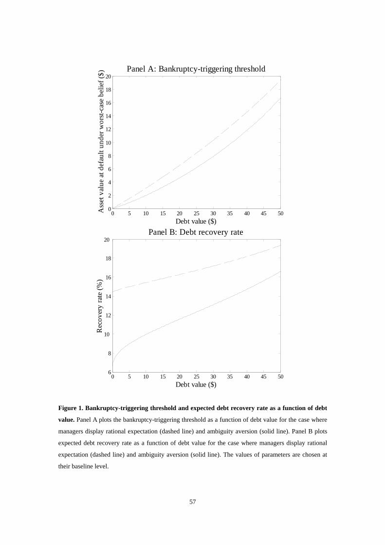
57

0 5 10 15 20 25 30 35 40 45 500

2

4

6

8

10

12

14

16

18

20Panel A: Bankruptcy-triggering threshold

Debt value ($)

Ass

et v

alue

at d

efau

lt un

der

wor

st-c

ase

belie

f ($

)

0 5 10 15 20 25 30 35 40 45 506

8

10

12

14

16

18

20 Panel B: Debt recovery rate

Debt value ($)

Rec

over

y ra

te (

%)

Figure 1. Bankruptcy-triggering threshold and expected debt recovery rate as a function of debt

value. Panel A plots the bankruptcy-triggering threshold as a function of debt value for the case where

managers display rational expectation (dashed line) and ambiguity aversion (solid line). Panel B plots

expected debt recovery rate as a function of debt value for the case where managers display rational

expectation (dashed line) and ambiguity aversion (solid line). The values of parameters are chosen at

their baseline level.

58

0 50 100 150 200 250 300

10

20

30

40

50

60

70

80

90

100 Panel A: Cumulative default probability

Time (year)

Def

ault

pro

babi

lity

(%

)

0 50 100 150 200 250 300

0.5

1

1.5

2

2.5

3

3.5

4 Panel B: Distribution of default probability-density

Time (year)

Def

ault

den

sity

(%

)

Figure 2. Subjective cumulative default probabilities and probability-density distribution. Panel A

plots the subjective cumulative default probabilities as a function of time for the case where managers

display ambiguity aversion (solid line) and rational expectation (dashed line). Panel B plots the default

probability-density as a function of time for the case where managers display ambiguity aversion (solid

line) and rational expectation (dashed line). The coupon is chosen to match the debt value at $50. The

values of parameters are chosen at their baseline level.

59

0 2 4 6 8 100

5

10

15

20

25

30

35Panel A: Asset risk

Time (year)

Cum

ulat

ive

defa

ult r

ate

(%)

0 2 4 6 8 100

1

2

3

4

5

6

7

8Panel B: Arbitrage-attitude

Time (year)

Cum

ulat

ive

defa

ult r

ate

(%)

0 2 4 6 8 100

1

2

3

4

5Panel C: Informational constraint

Time (year)

Cum

ulat

ive

defa

ult r

ate

(%)

0 2 4 6 8 100

1

2

3

4

5

6

7Panel D: Market index-Sharpe ratio

Time (year)

Cum

ulat

ive

defa

ult r

ate

(%)

Figure 3. Cumulative default probabilities as a function of time at optimal leverage. The lines in

each panel plot the cumulative default probabilities at optimal leverage given a range of time from 0 to

10 years. Panel A plots the probability curve for firm with three different levels of asset risk V : 20%

(solid line), 25% (dotted line), and 30% (dash-dotted line). Panel B plots the probability curve for firm

with three different levels of investors’ intention to arbitrage : 1 (dash-dotted line), 2 (solid line), and

3 (dotted line). Panel C plots the probability curve for firm with three different levels of the assets’ cor-

relation with market : 0.9 (solid line), 0.7 (dash-dotted line), and 0.5 (dotted line). Panel D plots the

probability curve for firm facing three different levels of market index Sharpe ratio Sh : 0.55 (dotted

line), 0.15 (dash-dotted line), and 0.33 (solid line). The values of parameters are chosen at their base-

line level. The coupons are chosen to maximize the firm’s total levered value under a worst-case belief

about the asset return.

60

0 20 40 60 80 100 100

102.5

105

107.5

110

112.5

115

Leverage ratio (%)

Tot

al f

irm

val

ue (

$)

Figure 4. Total firm value as a function of leverage. The lines plot the total firm value as a function

of leverage ratio for the case where managers display rational expectation (dashed line) and ambiguity

aversion (solid line). The values of parameter are assumed to be chosen at their baseline level.

61

0.2 0.25 0.3 0.35 0.444.5

45

45.5

46

46.5

47

47.5

48

48.5Panel A: Asset risk

Aggregate asset risk

Lev

erag

e ra

tio

(%)

1 1.5 2 2.5 347

47.5

48

48.5

49

49.5

50

50.5

51 Panel B: Arbitrage-attitude

Upper limit of Sharpe ratios/market index-Sharpe ratio

Lev

erag

e ra

tio

(%)

0 0.2 0.4 0.6 0.8 144

46

48

50

52

54

56

58

60 Panel C: Informational constraint

Correlation-coefficient

Lev

erag

e ra

tio

(%)

0.15 0.2 0.25 0.3 0.35 0.4 0.45 0.5 0.5547.5

48

48.5

49

49.5

50 Panel D: Market index-Sharpe ratio

Sharpe ratio

Lev

erag

e ra

tio

(%)

Figure 5. Optimal leverage ratio as a function of model parameters. The lines plot optimal leverage

ratio as a function of aggregate asset risk V in Panel A, investors’ intention to arbitrage in Panel

B, asset’s correlation with market in Panel C, and market index Sharpe ratio Sh in Panel D. The

values of parameters are chosen at their baseline level.

62

0 20 40 60 80 100 0

20

40

60

80

100Panel A: Base case

Leverage ratio (%)

Deb

t val

ue (

$)

60 65 70 75 80 85 90 95 100 60

65

70

75

80


Leverage ratio (%)D

ebt v

alue

($)

60 65 70 75 80 85 90 95 100 65

70

75


Leverage ratio (%)

Deb

t val

ue (

$)

60 65 70 75 80 85 90 95 100 65

70

75

80


Leverage ratio (%)

Deb

t val

ue (

$)

Figure 6. Debt value as a function of leverage with different combination of model parameters.

Lines in each panel plot the debt value as a function of leverage ratio. Panel A plots the debt value for

the case where managers display ambiguity aversion (solid line) and rational expectation (dashed line).

Panel B plots the debt value with three different levels of investors’ intention to arbitrage : 1 (dotted

line), 2 (solid line), and 3 (dash-dotted line). Panel C plots the debt value given three different levels of

the asset’s correlation with market : 0.9 (solid line), 0.8 (dash-dotted line), and 0.7 (dotted line). Pa-

nel D plots the debt value with three different levels of market index Sharpe ratio Sh : 0.15 (dotted line),

0.33 (solid line), and 0.55 (dash-dotted line). The parameter values are chosen at their baseline level.

63

0 5 10 15 20 25 30 35 40 0

50

100

150

200

250

300Panel A: Investment-grade bonds

Leverage ratio (%)

Cre

dit s

prea

d (b

ps)

45 50 55 60 65 70 75 80 850

100

200

300

400

500

600

700

800

900Panel B: Speculative-grade bonds

Leverage ratio (%)

Cre

dit s

prea

d (b

ps)

Figure 7. Credit spread as a function of leverage ratio. The lines plot credit spread as a function of

leverage for the case where managers display ambiguity aversion (solid line) and rational expectation

(dashed line). The values of parameters are chosen at their baseline level.

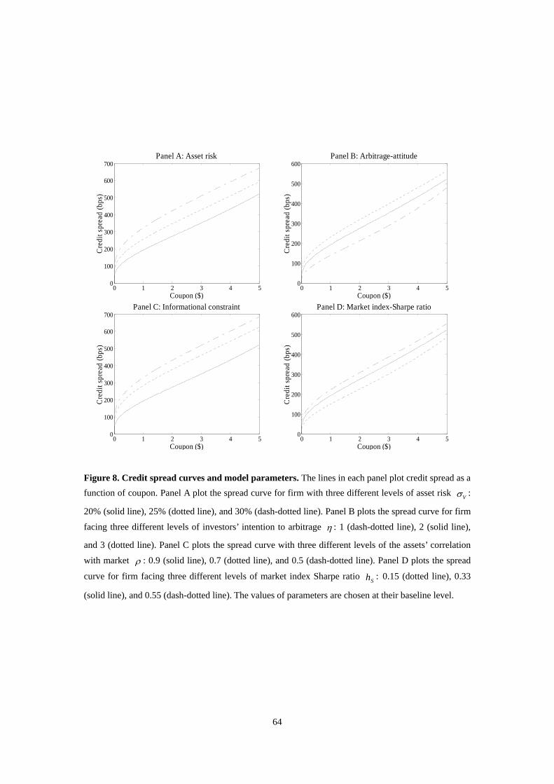
64

0 1 2 3 4 50

100

200

300

400

500

600

700Panel A: Asset risk

Coupon ($)

Cre

dit s

prea

d (b

ps)

0 1 2 3 4 50

100

200

300

400

500


Coupon ($)C

redi

t spr

ead

(bps

)

0 1 2 3 4 50

100

200

300

400

500

600


Coupon ($)

Cre

dit s

prea

d (b

ps)

0 1 2 3 4 50

100

200

300

400

500


Coupon ($)

Cre

dit s

prea

d (b

ps)

Figure 8. Credit spread curves and model parameters. The lines in each panel plot credit spread as a

function of coupon. Panel A plot the spread curve for firm with three different levels of asset risk V :

20% (solid line), 25% (dotted line), and 30% (dash-dotted line). Panel B plots the spread curve for firm

facing three different levels of investors’ intention to arbitrage : 1 (dash-dotted line), 2 (solid line),

and 3 (dotted line). Panel C plots the spread curve with three different levels of the assets’ correlation

with market : 0.9 (solid line), 0.7 (dotted line), and 0.5 (dash-dotted line). Panel D plots the spread

curve for firm facing three different levels of market index Sharpe ratio Sh : 0.15 (dotted line), 0.33

(solid line), and 0.55 (dash-dotted line). The values of parameters are chosen at their baseline level.

65

20 30 40 50 60 70 80 90 100 -250

-200

-150

-100

-50

0

50

100

150

Aggregate asset risk (%)

Val

ue-t

o-ri

sk s

ensi

tivity

Panel A: Debt and equity

0 20 40 60 80 100 -200

-150

-100

-50

0


Val

ue-t

o-ri

sk s

ensi

tivity

Panel B: Whole firm

Figure 9. Effects of a change in asset risk on equity, debt, and firm value at optimal leverage. The

lines in Panel A plot the partial derivative of equity value (solid and dotted lines) and partial derivative

of debt value (dashed and dash-dotted lines) with respect to aggregate asset risk V . The solid and

dashed lines are based on the case with ambiguity aversion; while the dotted and dash-dotted lines are

based on the standard case without ambiguity. The lines in Panel B plot the partial derivative of firm

value with respect to aggregate asset risk where the solid line is for the base case and the dashed line is

for the benchmark case. Coupons are chosen to maximize the firm’s total levered value under a worst-

case belief given 20% aggregate asset risk. The values of parameters are chosen at their baseline level.

66

0 5 10 15 20

20

40

60

80

100

Hedgeable risk (%)

Sen

sitiv

ity o

f ag

greg

ate

risk

to h

edgi

ng (

%)

Figure 10. Hedging efficiency with different levels of informational constraints. The lines plot the

partial derivative of aggregate asset risk V with respect to firm’s hedgeable (systematic) risk

VB

under four different levels of asset’s correlation with market : 0.9 (solid line), 0.7 (dashed line), 0.5

(dotted line), and 0.3 (dash-dotted line). The value of non-hedgeable risk VW is chosen to match the

initial aggregate asset risk at 20%.

67

0 10 20 30 40 505

10

15

20

25

30

35

40

45Panel A: Duration under ambiguity aversion

Debt value ($)

Dur

atio

n

0 10 20 30 40 5066.6

66.8

67

67.2

67.4

67.6

67.8

68

68.2Panel B: Duration under ambiguity loving

Debt value ($)

Dur

atio

n

1 1.2 1.4 1.6 1.8 2 -30

-20

-10

0

10

20

30

40

50 Panel C: Debt return and risk-free interest rate

Risk-free interest rate (%)

Deb

t ret

urn

(%)

20 30 40 50 60 70 80 90 100 -250

-200

-150

-100

-50

0

50

100

150

200Panel D: Asset substitution effect


Val

ue-t

o-ri

sk s

ensi

tivi

ty

Figure 11. Bond hedging and agency problem under different ambiguity attitudes. The solid line

in Panel A and B plots the duration as a function of debt value under ambiguity aversion and ambiguity

loving respectively. Panel C plots the relation between the returns on debt value and risk-free interest

rate. The solid line is based on a coupon choice to match debt value at $50 under ambiguity aversion;

the dashed line is based on a coupon choice to match debt value at $50 under ambiguity loving; the dot-

ted line is based on a coupon choice to match debt value at $30 under ambiguity loving; and the dash-

dotted line is based on a coupon choice to match debt value at $30 under ambiguity aversion. Panel D

plots the partial derivative of equity value (solid and dotted lines) and debt value (dashed and dash-dot

-ted lines) with respect to aggregate asset risk at optimal leverage. The solid and dashed lines are based

on the ambiguity-averse case. The dotted and dash-dotted lines are based on the ambiguity-loving case.

Coupons are chosen to maximize the firm’s value under the worst/best-case (ambiguity-averse/loving)

belief given 20% asset risk. The values of parameters are assumed to be chosen at their baseline level.

68

Table 1: Model Outputs at Optimal Capital Structure This table presents the comparative statics of model outputs at optimal capital structure with respect to

the factors of ambiguity (panels B, C, F, and G) and information constraint (panels D and E). Columns

from left to right respectively report the type of models, the ratio of debt to total firm value, the credit

spread of debt over risk-free rate, the ratio of expected recovery value to debt par, the debt’s face value,

the market value of equity, the value of net tax benefits, and 10-year cumulative default probabilities.

Ambiguity-

attitude

Leverage

ratio

Yield

spread

Debt reco-

very rate

Debt

value

Equity

value

Net tax

benefits

10-yr default

rate

Panel A: Base case

Aversion 48.36% 279 bps 17.19% $52.47 $56.02 8.49% 4.91%

N/A 57.55% 76 bps 21.83% $65.27 $48.14 13.41% 5.56%

Panel B: Conservative arbitrage-attitude 3 (Base: 2 )

Aversion 47.38% 348 bps 16.68% $51.18$ $56.85 8.04% 7.23%

N/A 57.55% 76 bps 21.83% $65.27$ $48.14 13.41% 5.56%

Panel C: Ambitious arbitrage-attitude 1 (Base: 2 )

Aversion 50.55% 188 bps 18.31% $55.38 $54.17 9.55% 3.26%

N/A 57.55% 76 bps 21.83% $65.27 $48.14 13.41% 5.56%

Panel D: Low degree of informational constraint 0.7 (Base: 0.9 )

Aversion 46.67% 416 bps 16.32% $50.27 $57.45 7.72% 4.83%

N/A 57.55% 76 bps 21.83% $65.27 $48.14 13.41% 5.56%

Panel E: Moderate degree of informational constraint 0.5 (Base: 0.9 )

Aversion 46.12% 486 bps 16.04% $49.58 $57.91 7.48% 2.50%

N/A 57.55% 76 bps 21.83% $65.27 $48.14 13.41% 5.56%

Panel F: High market-index Sharpe ratio 0.55Sh (Base: 0.33Sh )

Aversion 47.58% 332 bps 16.79% $51.44 $56.68 8.13% 6.59%

N/A 57.55% 76 bps 21.83% $65.27 $48.14 13.41% 5.56%

Panel G: Low market-index Sharpe ratio 0.15Sh (Base: 0.33Sh )

Aversion 49.98% 207 bps 18.02% $54.61 $54.65 9.26% 3.48%

N/A 57.55% 76 bps 21.83% $65.27 $48.14 13.41% 5.56%

69

Table 2: Data Definitions

Variable (Data Source) Variable Definition

Financial Indicators (Compustat):

Book debt Long term debt + Debt in current liabilities

Book equity Assets total – Book debt

Leverage Book debt / (Assets total – Book equity + Market value)

Tangibility 0.715 * Receivables + 0.547 * Inventory + 0.535 *Capital

Effective tax rate Total tax payments / Net pretax income

Interest payments Total interest expenses * adj. factor (see footnote 15)

Volatility, Sharpe ratio, Value-Risk Elasticity, and Beta (3000 Xtra, Reuters/Datastream):

Equity volatility Standard deviation of monthly equity return

Index volatility Standard deviation of monthly S&P 500 index return

Sharpe ratio of market index Excess index return / Standard deviation of index return

Market model beta Market model regression beta on monthly equity return

Equity value-risk elasticity OLS equity return rate-percentage changes in the firm’s risk

regression coefficient

Debt value-risk elasticity OLS debt return rate-percentage changes in the firm’s risk

regression coefficient

Economic indicator (FED):

Term premium Difference between 30-year and 5-year government bond yield

Slope of treasury yield curve Difference between 10-year and 2-year government bond yield

70

Table 3: Summary Statistics The table presents the descriptive statistics for main variables used in estimations. The sample of S&P

500 firms is based on Compustat, Datastream and 3000 Xtra of Thomson Reuters, covering the period

of January 2, 1992 to December 31, 2011. Last 3-year average and current credit rating data is acquired

from Compustat. The detailed definition of other variables is available in Table 2.

Panel A: Descriptive Statistics

Quantitative variable Mean S.D. 25% Median 75% N

Equity Std. Dev. (%) 31.043 10.558 23.966 29.680 36.387 274

Effective tax rate (%) 33.377 6.381 29.967 33.783 37.589 274

Tangibility-asset ratio (%) 33.378 9.880 26.687 34.394 41.095 274

Market-model beta 1.011 0.442 0.669 0.963 1.312 274

Market leverage (%) 17.640 11.941 8.735 15.068 24.093 274

Total interest expenses-

book debt ratio (%) 8.241 3.120 6.439 7.430 9.242 274

Val.-risk elasticity (equity) -0.220 0.185 -0.323 -0.211 -0.124 274

Val.-risk elasticity (debt) -0.029 0.037 -0.042 -0.022 -0.005 133

Panel B: Frequency (numbers of firm) distribution

Qualitative variable AAA AA A BBB BB B/CCC N.A.

Last 3-yr avg. credit rating 4 14 87 104 35 6 24

Current credit rating 3 12 83 119 32 7 18

71

Table 4: Parameter Estimates and Target Financial Variables The table compiles the estimates of firm-specific parameters, non-firm-specific parameters, and target

financial variables in Panel A, B, and C respectively. Asset aggregate risk is estimated by the monthly

volatility of equity return. Effective tax rate is estimated by using the ratio of tax payment to net pretax

income. Bankruptcy cost is estimated by the formula of assets’ abandonment value proposed by Berger

et al. (1996). Systematic risk proportion is estimated using the ratio of the product of market beta and

market risk to firm’s total risk. Sharpe ratio of the market portfolio is estimated by the ratio of average

excess return on S&P 500 index to its standard deviation. Riskless rate is estimated by 1-year treasury

rate. Term premium on bonds is measured as the difference between 30-year and 10-year government

bond yield, as in Morellec et al. (2011). The slope of treasury yield curve is estimated by the difference

between 10-year and 2-year government bond yields, as in Collin-Dufresne et al. (2001). The detailed

definition of target financial variables is available in Table 2.

Panel A: Firm-specific parameters by leverage group

Items OverallLeverage group

< 8% 8-16% 16-24% 24-32% >32%

Asset aggregate risk (%) 31.043 31.087 30.090 32.937 30.455 30.624

Effective tax rate (%) 33.377 31.907 33.708 32.606 35.566 34.394

Bankruptcy cost rate (%) 57.401 51.042 57.869 58.805 61.965 60.778

Systematic risk proportion (%) 44.375 42.268 43.169 45.225 46.770 47.232

Panel B: Non-firm-specific parameters

Market-portfolio

Sharpe ratio One-year treasury rate (%) Term premium (bps)

The slope of treasury

yield curve (bps)

0.187 3.524 116 118

Panel C: Target variables

Leverage (%) Yield spread (bps) Debt value-risk

elasticity

Equity value-risk

elasticity

17.640 (mean)

11.941 (S.D.)

262 (mean)

123 (S.D.)

-0.029(mean)

0.037(S.D.)

-0.220 (mean)

0.185 (S.D.)

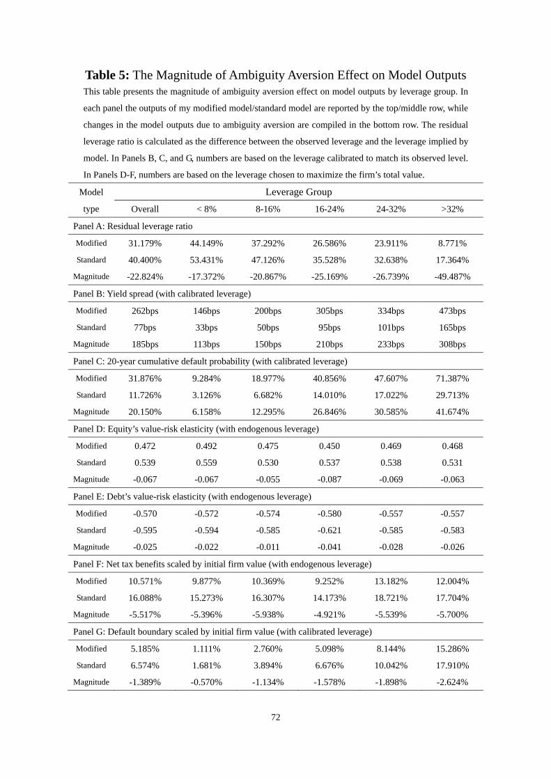
72

Table 5: The Magnitude of Ambiguity Aversion Effect on Model Outputs This table presents the magnitude of ambiguity aversion effect on model outputs by leverage group. In

each panel the outputs of my modified model/standard model are reported by the top/middle row, while

changes in the model outputs due to ambiguity aversion are compiled in the bottom row. The residual

leverage ratio is calculated as the difference between the observed leverage and the leverage implied by

model. In Panels B, C, and G, numbers are based on the leverage calibrated to match its observed level.

In Panels D-F, numbers are based on the leverage chosen to maximize the firm’s total value.

Model

type

Leverage Group

Overall < 8% 8-16% 16-24% 24-32% >32%

Panel A: Residual leverage ratio

Modified 31.179% 44.149% 37.292% 26.586% 23.911% 8.771%

Standard 40.400% 53.431% 47.126% 35.528% 32.638% 17.364%

Magnitude -22.824% -17.372% -20.867% -25.169% -26.739% -49.487%

Panel B: Yield spread (with calibrated leverage)

Modified 262bps 146bps 200bps 305bps 334bps 473bps

Standard 77bps 33bps 50bps 95bps 101bps 165bps

Magnitude 185bps 113bps 150bps 210bps 233bps 308bps

Panel C: 20-year cumulative default probability (with calibrated leverage)

Modified 31.876% 9.284% 18.977% 40.856% 47.607% 71.387%

Standard 11.726% 3.126% 6.682% 14.010% 17.022% 29.713%

Magnitude 20.150% 6.158% 12.295% 26.846% 30.585% 41.674%

Panel D: Equity’s value-risk elasticity (with endogenous leverage)

Modified 0.472 0.492 0.475 0.450 0.469 0.468

Standard 0.539 0.559 0.530 0.537 0.538 0.531

Magnitude -0.067 -0.067 -0.055 -0.087 -0.069 -0.063

Panel E: Debt’s value-risk elasticity (with endogenous leverage)

Modified -0.570 -0.572 -0.574 -0.580 -0.557 -0.557

Standard -0.595 -0.594 -0.585 -0.621 -0.585 -0.583

Magnitude -0.025 -0.022 -0.011 -0.041 -0.028 -0.026

Panel F: Net tax benefits scaled by initial firm value (with endogenous leverage)

Modified 10.571% 9.877% 10.369% 9.252% 13.182% 12.004%

Standard 16.088% 15.273% 16.307% 14.173% 18.721% 17.704%

Magnitude -5.517% -5.396% -5.938% -4.921% -5.539% -5.700%

Panel G: Default boundary scaled by initial firm value (with calibrated leverage)

Modified 5.185% 1.111% 2.760% 5.098% 8.144% 15.286%

Standard 6.574% 1.681% 3.894% 6.676% 10.042% 17.910%

Magnitude -1.389% -0.570% -1.134% -1.578% -1.898% -2.624%

73

Table 6: Goodness-of-Fit for Leverage The table presents the comparison of goodness-of-fit for leverage in two ways: moments (Panel A) and

prediction errors (Panel B). Columns in the top panel reports the value of various statistical moments in

the data and models, including mean, standard deviation, median, skew, and kurtosis (from left to right).

In the bottom panel, MAE reports the mean of absolute error; RMSE reports the root of mean squared

error; and Range shows the distance between max and min error. The t-statistic tests whether the errors

of the chosen model are lower than its alternative model. The associated p-value gives the testing result.

Panel A: Moments

Items Mean S.D. Median Skew Kurtosis

Full sample:

Empirical data 0.176 0.119 0.151 1.180 4.563

Modified model 0.488 0.099 0.499 -0.594 8.071

Standard model 0.581 0.101 0.587 -1.015 8.430

Low-levered firms (< 17%):

Empirical data 0.095 0.042 0.095 0.007 2.005

Modified model 0.490 0.077 0.502 -0.441 3.034

Standard model 0.584 0.083 0.589 -0.501 3.584

Highly-levered firms (> 17%):

Empirical data 0.287 0.100 0.258 1.373 5.259

Modified model 0.485 0.123 0.498 -0.542 7.360

Standard model 0.575 0.123 0.583 -1.085 8.222

Panel B: Prediction errors

Items MAE RMSE Range t-statistic p-value

Full sample:

Modified model 0.322 0.347 1.037 -35.998 0.999

Standard model 0.410 0.433 1.008 35.998 0


Modified model 0.395 0.405 0.489 -27.090 0.999

Standard model 0.489 0.498 0.547 27.090 0


Modified model 0.222 0.247 1.037 -23.618 0.999

Standard model 0.303 0.325 0.961 23.618 0

74

Table 7: Goodness-of-Fit for Yield Spread The table gives the comparison of goodness-of-fit for yield spread in two ways: moments (Panel A) and

prediction errors (Panel B). Columns in the top panel reports the value of various statistical moments in

the data and models, including mean, standard deviation, median, skew, and kurtosis (from left to right).

In the bottom panel, MAE reports the mean of absolute error; RMSE reports the root of mean squared

error; and Range shows the distance between max and min error. The t-statistic tests whether the errors

of the chosen model are lower than its alternative model. The associated p-value gives the testing result.

Panel A: Moments

Items Mean S.D. Median Skew Kurtosis

Full sample:

Empirical data 0.0262 0.0123 0.0231 2.5584 12.3052

Modified model 0.0262 0.0197 0.0226 1.9161 8.5451

Standard model 0.0077 0.0116 0.0044 4.1622 28.4176


Empirical data 0.0226 0.0079 0.0206 2.5900 13.3510

Modified model 0.0195 0.0154 0.0163 2.8064 16.1584

Standard model 0.0055 0.0108 0.0026 6.2918 55.2550


Empirical data 0.0311 0.0152 0.0251 2.0043 8.3649

Modified model 0.0354 0.0214 0.0316 1.5118 6.5682

Standard model 0.0108 0.0118 0.0076 2.4770 10.1205

Panel B: Prediction errors

Items MAE RMSE Range t-statistic p-value

Full sample:

Modified model 0.0123 0.0169 0.1548 -3.0574 0.999

Standard model 0.0193 0.0220 0.1490 3.0574 0.001


Modified model 0.0105 0.0141 0.1317 -2.1501 0.984

Standard model 0.0183 0.0201 0.1314 2.1501 0.016


Modified model 0.0146 0.0201 0.1290 -2.5656 0.995

Standard model 0.0206 0.0243 0.0747 2.5656 0.005

75

Table 8: Goodness-of-Fit for Value-Risk Elasticity The table gives the comparison of prediction-error between my modified model and standard model for

value-risk elasticity. MAE reports the mean of absolute error. RMSE reports the root of mean squared

error. The t-statistic tests check whether the prediction errors of the chosen model are smaller than the

alternative model. The associated p-value displays the test result. In calculating MAE and RMSE on the

debt’s value-to-risk elasticity, the target elasticity for firms without analyzable bond data is set at -0.029,

which equals the mean of bond sample.

Items MAE

(debt)

RMSE

(debt)

t-statistic

(debt)

p-value

(debt)

MAE

(equity)

RMSE

(equity)

t-statistic

(equity)

p-value

(equity)

Full sample:

Modified 0.542 0.545 -3.061 0.999 0.693 0.728 -9.153 0.999

Standard 0.566 0.586 3.061 0.001 0.760 0.814 9.153 0


Modified 0.548 0.550 -2.221 0.987 0.693 0.723 -6.417 0.999

Standard 0.572 0.592 2.221 0.013 0.758 0.810 6.417 0


Modified 0.533 0.539 -2.132 0.983 0.694 0.735 -6.711 0.999

Standard 0.556 0.579 2.132 0.017 0.763 0.819 6.711 0

corporate financing under ambiguity: a utility-free ... · corporate financing under ambiguity: a...

Documents